A novel generalization of Bézier curve and surface

Journal of Computational and Applied Mathematics 217 (2008) 180–193www.elsevier.com/locate/cam

A novel generalization of Bézier curve and surface

Xi-An Hana,b,∗, YiChen Maa, XiLi Huangc

aSchool of Science, XiAn JiaoTong University, ShaanXi 710049, PR ChinabDepartment of Basic Theories, The Academy of Equipment Command & Technology, Beijing 101416, PR China

cDepartment of Experiment Command, The Academy of Equipment Command & Technology, Beijing 101416, PR China

Received 25 December 2006; received in revised form 25 June 2007

Abstract

A new formulation for the representation and designing of curves and surfaces is presented. It is a novel generalization of Béziercurves and surfaces. Firstly, a class of polynomial basis functions with n adjustable shape parameters is present. It is a naturalextension to classical Bernstein basis functions. The corresponding Bézier curves and surfaces, the so-called Quasi-Bézier (i.e.,Q-Bézier, for short) curves and surfaces, are also constructed and their properties studied. It has been shown that the main advantagecompared to the ordinary Bézier curves and surfaces is that after inputting a set of control points and values of newly introduced n

shape parameters, the desired curve or surface can be flexibly chosen from a set of curves or surfaces which differ either locally orglobally by suitably modifying the values of the shape parameters, when the control polygon is maintained. The Q-Bézier curve andsurface inherit the most properties of Bézier curve and surface and can be more approximated to the control polygon. It is visiblethat the properties of end-points on Q-Bézier curve and surface can be locally controlled by these shape parameters. Some examplesare given by figures.© 2007 Elsevier B.V. All rights reserved.

MSC: primary 65D17;65D10; secondary 42A10

Keywords: Computer aided geometric design; Generalized Bernstein basis functions; Bézier curve/surface patches; Q-Bézier curve/surfacepatches; Shape parameters

1. Introduction

Parametric representation of curves and surfaces is widely used in Computer Aided Geometric Design (CAGD)and Computer Graphics (CG) to model interactively various surfaces by means of surface patches. When representinga parametric curve or surface, it is important which basis functions are used if we wish to preserve the shape ofthe curve or surface. For these reasons the Bernstein–Bézier curve and surface representation plays a significant rolein CAGD&CG [5,14]. Many authors have studied several kinds of spline for curve and surface design and control[2,3,8–10,15,16,18,24]. In general, the common spline interpolation is the fixed interpolation which means that theshape of the interpolating curve or surface is fixed for the given interpolating data and control polygon, since theinterpolating function is unique for the given control points. If one wishes to modify the shape of the interpolatingcurve, the interpolating data need to be changed. An important question is how can the shape of the curve be modified

∗ Corresponding author. Tel.: +86 029 82671828.E-mail address: [email protected] (X.-A. Han).

0377-0427/$ - see front matter © 2007 Elsevier B.V. All rights reserved.doi:10.1016/j.cam.2007.06.027

http://www.elsevier.com/locate/cam

mailto:[email protected]

X.-A. Han et al. / Journal of Computational and Applied Mathematics 217 (2008) 180–193 181

under the condition that the given data and control polygon are not changed? That is a important problem in CAGD&CG.Theoretically speaking, it is contradictory to the uniqueness of the interpolating function for the given interpolatingdata and control polygon.

The rational Bézier model is a powerful tool for constructing free-form curves and surfaces. In recent years, therational spline with parameters has received attention in the literature [4,6,11]. For the given interpolating data, thechange of the parameters causes the change of the interpolating curve, so that the interpolating curve may be modified tobe the needed shape if suitable parameters exist. That is, the uniqueness of the interpolating function for the given datais replaced by the uniqueness of the interpolating curve for the given data and the selected parameters. However, it hasmany shortcomings due to its rational form and nonpolynomial form. For instance, repeated differentiation producescurves of very high degree.

Bernstein polynomials and Bézier curves are of fundamental importance for CAGD &CG. They are used for thedesign of curves and they are the starting point for several generalizations [1,6,7,12,13,17,19–23,25,26]: in particularto higher dimensions and to B-splines. Powerful algorithms are available for both their algebraic construction andtheir visualization, and their basic theory (explained beautifully in Farin’s book [5]) has been examined repeatedlyfrom different new angles: see, e.g., for the “basis function” point of view, many bases are presented in new spacesother than the polynomial space [12,13,19,20,22,25,26], [1] for the “natural generalization of Bézier curves”, [7] for“barycentric” and [21] for “blossoming”. Although these algorithms are very effective and widely used in practice,they have a drawback: they are not able to control the shape of the corresponding curves keeping the control polygonunchanged.

In the present paper, we introduce an approach to the generalization of Bernstein polynomials and Bézier curvesand surfaces which seems to be entirely new. It is based on the novel ideas that the shape of the curves and surfaces iscontrolled by the control edges of the control polygon, not by the control points. These curves and surfaces have moresimplify form and clear geometric meaning than rational Bézier curves and surfaces.

The present paper is organized as follows. In Section 2, a class of polynomial basis functions with adjustable shapeparameters is constructed and the properties of the basis functions are shown. The corresponding Q-Bézire curvesand surfaces are presented and their properties studied in Sections 3 and 6, respectively. In Section 4 the effect ofthe shape of the curve by the shape parameters is given. The composite Q-bézier curves are discussed in Section 5as well.

2. Generalized Bernstein basis function

Firstly, the definition of generalized Bernstein basis functions is constructed as follows.

Definition 2.1. For every nature number n(n�2) and n arbitrarily selected real values of �i , i = 1, 2, . . . , n, thefollowing polynomial functions

⎧⎪⎪⎪⎪⎪⎪⎪⎪⎪⎪⎪⎪⎨⎪⎪⎪⎪⎪⎪⎪⎪⎪⎪⎪⎪⎩

bn0(t) = (1 − t)n(1 − �1t),

bni (t) = t i (1 − t)n−i

((n

i

)+ �i − �i t − �i+1t

), i = 1, . . . ,

[n

2

]− 1,

bn

[n2 ](t) = t[n2 ]

(1 − t)n−[n2 ]

((n[n2

])

+ �[n2 ] − �[n2 ]t + �[n2 ]+1t

),

bni (t) = t i (1 − t)n−i

((n

i

)− �i + �i t + �i+1t

), i =

[n

2

]+ 1, . . . , n − 1,

bnn(t) = tn(1 − �n + �nt)

(2.1)

are called the generalized Bernstein polynomials of degree n associated with the shape parameters {�i}ni=1, where

�i ∈[− (

ni

),(

ni−1

)], i = 1, 2, . . . , [n

2 ], �i ∈[−

(n

i−1

),(

ni

)], i = [n

2 ] + 1, . . . , n and [n2 ] =

{ n2 , if n is even,

n+12 , if n is odd.

It is obvious, for �i = 0, i = 1, 2, . . . , n, the basis functions are classical Bernstein polynomials of degree n.

182 X.-A. Han et al. / Journal of Computational and Applied Mathematics 217 (2008) 180–193

Theorem 2.1. The generalized Bernstein basis functions of degree n associated with the shape parameters {�i}ni=1(2.1) have the following properties:

(a) nonnegativity: bni (t)�0, i = 0, 1, . . . , n;

(b) partition of unity:∑n

i=0 bni (t) ≡ 1;

(c) symmetry: for i = 0, 1, . . . , n;

bni

(t; �1, . . . , �[n2 ]−1, �[n2 ], �[n2 ]+1, . . . , �n

)= bn

n−i

(1 − t; �n, . . . , �[n2 ]+1, (−1)n�[n2 ], �[n2 ]−1, . . . , �1

).

Proof. (a) For t ∈ [0, 1] and the range of �i , i =1, . . . , n in Definition 2.1, then 1−�1t �0,(

ni

)+�i −�i t −�i+1t �0,(n

[n2 ]

)+ �i − �i t + �i+1t �0,

(ni

) − �i + �i t + �i+1t �0 and 1 − �nt �0. It is obvious that bni (t)�0, i = 0, 1, . . . , n.

(b)∑n

i=0 bni (t) = ∑n

i=0

(ni

)t i (1 − t)n−i ≡ 1.

(c) If n is even, the symmetry of {bni (t)}ni=0 holds obviously.

For n is odd,

−(

n[n2

] − 1

)� − �[n2 ] �

(n[n2

])

,

because n − [n2 ] = [n

2 ] − 1, hence,

−(

n[n2

])

� − �[n2 ] �(

n[n2

] − 1

)

and for i = 0, 1, . . . , n,

bni

(t; �1, . . . , �[n2 ]−1, �[n2 ], �[n2 ]+1, . . . , �n

)= bn

n−i

(1 − t; �n, . . . , �[n2 ]+1, (−1)n�[n2 ], �[n2 ]−1, . . . , �1

).

Obviously when n is odd, the symmetry of {bni (t)}ni=0 holds as well. �

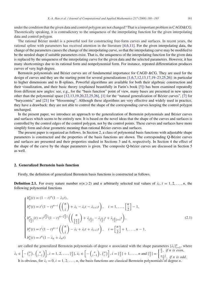
Fig. 1 shows the curves of the generalized polynomial basis functions for n = 2 and �1 = −2, �2 = 1 (dashed lines),�1 = −1, �2 = −1 (solid lines) and �1 = 1, �2 = −2 (dotted lines), respectively.

0 0.1 0.2 0.3 0.4 0.5 0.6 0.7 0.8 0.9 10

0.1

0.2

0.3

0.4

0.5

0.6

0.7

0.8

0.9

1

Fig. 1. The quadratic generalized Bernstein basis functions.


0 0.1 0.2 0.3 0.4 0.5 0.6 0.7 0.8 0.9 10

0.1

0.2

0.3

0.4

0.5

0.6

0.7

0.8

0.9

1

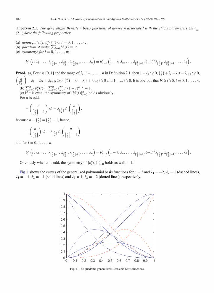
Fig. 2. The cubic generalized Bernstein basis functions.

Fig. 2 shows the curves of the generalized polynomial basis functions for n=3 and (�1, �2, �3)= (−2, 0, 1) (dashedlines), for (�1, �2, �3) = (−1, 1, −1) (solid lines) and for (�1, �2, �3) = (1, −2, −2) (dotted lines), respectively.

3. Construction of the Q-Bézier curve

Definition 3.1. Given points Pi (i = 0, 1, · · · , n) ∈ R2 or R3, then

r(t) =n∑

i=0

Pibni (t), t ∈ [0, 1] (3.1)

is called Q-Bézier curve with shape parameters, where �i ∈[− (

ni

),(

ni−1

)], i=1, 2, . . . , [n

2 ], �i ∈[−

(n

i−1

),(

ni

)],

i = [n2 ] + 1, . . . , n.

From the definition of the basis functions (2.1), some properties of Q-Bézier curve can be obtained as follows:

Theorem 3.1. The Q-Bézier curves (3.1) have the following properties:

(a) Terminal properties:

r(0) = P0, r(1) = Pn. (3.2)

Let ai = Pi − Pi−1, i = 1, 2, . . . , n, then

r′(0) = (n + �1)a1, r′(1) = (n + �n)an, (3.3)

r′′(0) = n(n − 1)(a2 − a1) − 2n�1a1 + 2�2a2, (3.4)

r′′(1) = n(n − 1)(an − an−1) + 2n�nan + 2�n−1an−1. (3.5)

(b) Symmetry: Both P0, P1, . . . , Pn and Pn, Pn−1, . . . , P0 define the same Q-Bézier curve in a different parametrization,i.e.,

r(t; {�j }nj=1; {Pi}ni=0) = r(

1 − t; �n, . . . , �[ n2 ]+1, (−1)n�[n2 ], �[n2 ]−1, . . . , �1; {Pn−i}ni=0

). (3.6)


(c) Geometric invariance: The shape of a Q-Bézier curve is independent of the choice of coordinates, i.e., Eq. (3.1)satisfies the following two equations:

r(t; {�j }nj=1; P0 + q, P1 + q, . . . , Pn + q) = r(t; {�j }nj=1; P0, P1, . . . , Pn) + q,

r(t; {�j }nj=1; P0 ∗ T, P1 ∗ T, · · · , Pn ∗ T) = r(t; {�j }nj=1; P0, P1, · · · , Pn) ∗ T, (3.7)

where q is an arbitrary vector in R2 or R3, and T is an arbitrary d × d matrix, d = 2 or 3.(d) Convex hull property:The entire Q-Bézier curve segment must lie inside its control polygon spanned by P0, P1, . . . , Pn.

4. Shape control of the Q-Bézier curve

For t ∈ (0, 1), we rewrite (3.1) as follows:

r(t) =n∑

i=0

PiBni (t) +

[n2 ]∑i=1

�i (1 − t)n+1−i t iai −n∑

i=[n2 ]+1

�i (1 − t)n+1−i t iai , (4.1)

where Bni (t) = (

ni

)(1 − t)n−i t i , i = 0, 1, . . . , n is classical Bernstein polynomials of degree n.

Obviously, shape parameters �i (i = 1, 2, . . . , n) only affect curve on the corresponding control edges ai (i =1, 2, . . . , n), i.e., the shape of the curve can be modified by the control edges of control polygon with altering thevalues of the corresponding shape parameters. In fact, from (4.1), we can also predict the following behaviors of thecurves.

The shape parameters �i , i = 1, 2, . . . , n serve to local control in the curves: as �i (i = 1, 2, . . . , [n2 ]) increases, the

curve moves in the direction of ai (i =1, 2, . . . , [n2 ]), as �i (i =1, 2, . . . , [n

2 ]) decreases, the curve moves in the oppositedirection of ai (i = 1, 2, . . . , [n

2 ]). The same effects on the edge ai (i = [n2 ] + 1, . . . , n) played by the corresponding

shape parameters �i (i = [n2 ] + 1, . . . , n).

The effect of the shape parameters of the Q-Bézier curves (3.1) is clear. Figs. 3–10 show the effects on shape of thecurve with altering the values of �i (i = 1, 2, . . . , n) for n = 3 and n = 4, respectively.

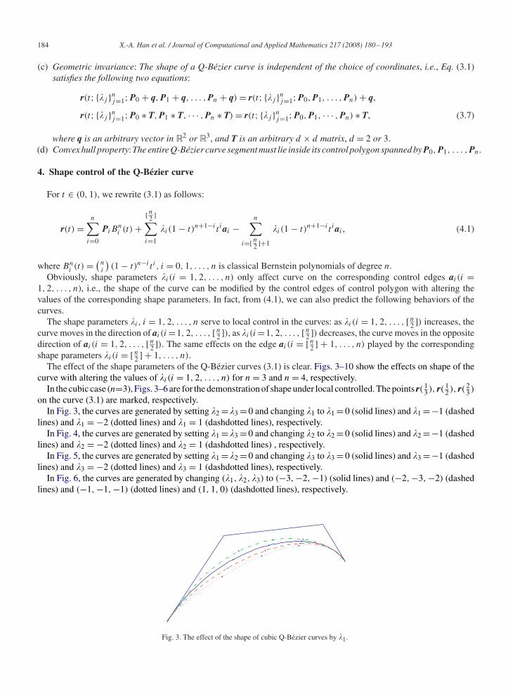
In the cubic case (n=3), Figs. 3–6 are for the demonstration of shape under local controlled. The points r( 13 ), r( 1

2 ), r( 23 )

on the curve (3.1) are marked, respectively.In Fig. 3, the curves are generated by setting �2 =�3 =0 and changing �1 to �1 =0 (solid lines) and �1 =−1 (dashed

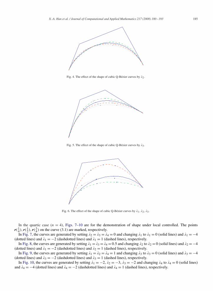
lines) and �1 = −2 (dotted lines) and �1 = 1 (dashdotted lines), respectively.In Fig. 4, the curves are generated by setting �1 =�3 =0 and changing �2 to �2 =0 (solid lines) and �2 =−1 (dashed

lines) and �2 = −2 (dotted lines) and �2 = 1 (dashdotted lines) , respectively.In Fig. 5, the curves are generated by setting �1 =�2 =0 and changing �3 to �3 =0 (solid lines) and �3 =−1 (dashed

lines) and �3 = −2 (dotted lines) and �3 = 1 (dashdotted lines), respectively.In Fig. 6, the curves are generated by changing (�1, �2, �3) to (−3, −2, −1) (solid lines) and (−2, −3, −2) (dashed

lines) and (−1, −1, −1) (dotted lines) and (1, 1, 0) (dashdotted lines), respectively.

Fig. 3. The effect of the shape of cubic Q-Bézier curves by �1.




Fig. 6. The effect of the shape of cubic Q-Bézier curves by �1, �2, �3.

In the quartic case (n = 4), Figs. 7–10 are for the demonstration of shape under local controlled. The pointsr( 1

4 ), r( 12 ), r( 3

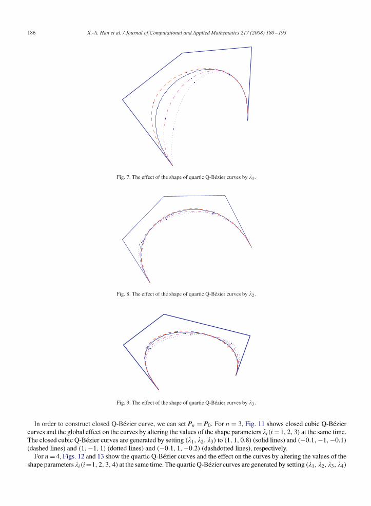
4 ) on the curve (3.1) are marked, respectively.In Fig. 7, the curves are generated by setting �2 = �3 = �4 = 0 and changing �1 to �1 = 0 (solid lines) and �1 = −4

(dotted lines) and �1 = −2 (dashdotted lines) and �1 = 1 (dashed lines), respectively.In Fig. 8, the curves are generated by setting �1 = �3 = �4 = 0.5 and changing �2 to �2 = 0 (solid lines) and �2 = −4

(dotted lines) and �1 = −2 (dashdotted lines) and �2 = 1 (dashed lines), respectively.In Fig. 9, the curves are generated by setting �1 = �2 = �4 = 1 and changing �3 to �3 = 0 (solid lines) and �3 = −4

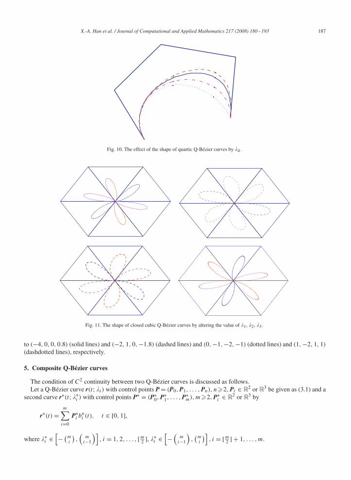
(dotted lines) and �3 = −2 (dashdotted lines) and �3 = 1 (dashed lines), respectively.In Fig. 10, the curves are generated by setting �1 = −2, �2 = −3, �3 = −2 and changing �4 to �4 = 0 (solid lines)

and �4 = −4 (dotted lines) and �4 = −2 (dashdotted lines) and �4 = 1 (dashed lines), respectively.


Fig. 7. The effect of the shape of quartic Q-Bézier curves by �1.



In order to construct closed Q-Bézier curve, we can set Pn = P0. For n = 3, Fig. 11 shows closed cubic Q-Béziercurves and the global effect on the curves by altering the values of the shape parameters �i (i =1, 2, 3) at the same time.The closed cubic Q-Bézier curves are generated by setting (�1, �2, �3) to (1, 1, 0.8) (solid lines) and (−0.1, −1, −0.1)

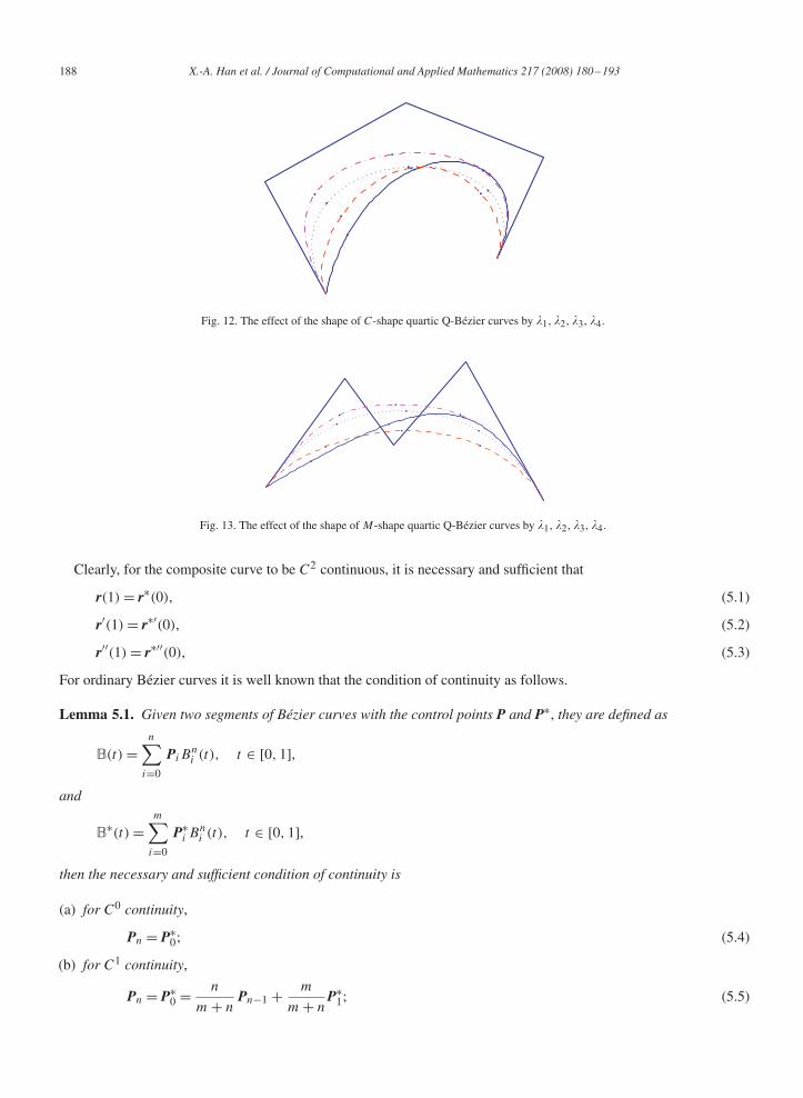
(dashed lines) and (1, −1, 1) (dotted lines) and (−0.1, 1, −0.2) (dashdotted lines), respectively.For n= 4, Figs. 12 and 13 show the quartic Q-Bézier curves and the effect on the curves by altering the values of the

shape parameters �i (i=1, 2, 3, 4) at the same time. The quartic Q-Bézier curves are generated by setting (�1, �2, �3, �4)



Fig. 11. The shape of closed cubic Q-Bézier curves by altering the value of �1, �2, �3.

to (−4, 0, 0, 0.8) (solid lines) and (−2, 1, 0, −1.8) (dashed lines) and (0, −1, −2, −1) (dotted lines) and (1, −2, 1, 1)

(dashdotted lines), respectively.

5. Composite Q-Bézier curves

The condition of C2 continuity between two Q-Bézier curves is discussed as follows.Let a Q-Bézier curve r(t; �i ) with control points P = (P0, P1, . . . , Pn), n�2, Pi ∈ R2 or R3 be given as (3.1) and a

second curve r∗(t; �∗i ) with control points P∗ = (P∗

0, P∗1, . . . , P∗

m), m�2, P∗i ∈ R2 or R3 by

r∗(t) =m∑

i=0

P∗i b

ni (t), t ∈ [0, 1],

where �∗i ∈

[− (

mi

),(

mi−1

)], i = 1, 2, . . . , [m

2 ], �∗i ∈

[−

(m

i−1

),(

mi

)], i = [m

2 ] + 1, . . . , m.


Fig. 12. The effect of the shape of C-shape quartic Q-Bézier curves by �1, �2, �3, �4.

Fig. 13. The effect of the shape of M-shape quartic Q-Bézier curves by �1, �2, �3, �4.

Clearly, for the composite curve to be C2 continuous, it is necessary and sufficient that

r(1) = r∗(0), (5.1)

r′(1) = r∗′(0), (5.2)

r′′(1) = r∗′′(0), (5.3)

For ordinary Bézier curves it is well known that the condition of continuity as follows.

Lemma 5.1. Given two segments of Bézier curves with the control points P and P∗, they are defined as

B(t) =n∑

i=0

PiBni (t), t ∈ [0, 1],

and

B∗(t) =m∑

i=0

P∗i B

ni (t), t ∈ [0, 1],

then the necessary and sufficient condition of continuity is

(a) for C0 continuity,

Pn = P∗0; (5.4)

(b) for C1 continuity,

Pn = P∗0 = n

m + nPn−1 + m

m + nP∗

1; (5.5)


(c) for C2 continuity,

P∗2 = n(n − 1)

m(m − 1)Pn−2 + 1

m(m − 1)[n(n+2m − 3)(Pn − Pn−1)+m(m−1)Pn − n(n − 1)Pn−1]. (5.6)

According to the terminal properties of Q-Bézier curves, the theorem below shows the condition of continuity of thecomposite Q-Bézier curves.

Theorem 5.1. Given two segments of Q-Bézier curves with the control points P and P∗, then the necessary and sufficientcondition of continuity is

(a) for C0 continuity,

Pn = P∗0; (5.7)

(b) for C1 continuity,

Pn = P∗0 = (n + �n)Pn−1 + (m + �∗

1)P∗1

m + n + �n + �∗1

; (5.8)

(c) for C2 continuity,

P∗2 = aPn−2 + b[c(Pn − Pn−1) + 2�n−1Pn−1 + 2�∗

2Pn]; (5.9)

where a = n(n−1)−2�n−1m(m−1)+2�∗

2, b = 1

m(m−1)+2�∗2, c = 4n2 + n�n − 2n + 2(n+�n)(�∗

2−m)

m+�∗1

.

Proof. All the formulas result from straightforward computations (a) is obvious.For (b), according to (5.2), (3.3) and (5.7),

(n + �n)(Pn − Pn−1) = (m + �∗1)(P

∗1 − P∗

0), (5.10)

(5.8) holds after simple reorganization.For (c), from (5.8),

P∗1 − P∗

0 = n + �n

m + �∗1(Pn − Pn−1). (5.11)

According to (5.3) and (3.4),

n(n − 1)[(Pn − Pn−1) − (Pn−1 − Pn−2)] + 2n�n(Pn − Pn−1) + 2�n−1(Pn−1 − Pn−2)

= m(m − 1)[(P∗2 − P∗

1) − (P∗1 − P∗

0)] − 2m�∗1(P

∗1 − P∗

0) + 2�∗2(P

∗2 − P∗

1). (5.12)

Substituting (5.7), (5.8) and (5.11) into (5.12), (5.9) can be obtained. �

Remark 5.1. The condition of C1 continuity (5.8) of Q-Bézier curves (3.1) is more flexible compared with the conditionof ordinary Bézier curves (5.5). Especially, when �n = �∗

1 the condition (5.8) is same as (5.5).

Remark 5.2. The condition of C2 continuity (5.9) of Q-Bézier curves (3.1) is more flexible compared with the conditionof ordinary Bézier curves (5.6). Especially, when �n−1 = �∗

2 = 0 the condition (5.9) is same as (5.6).

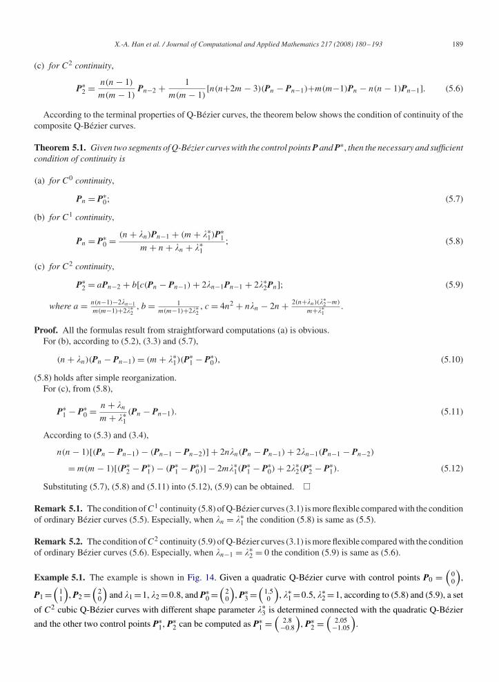
Example 5.1. The example is shown in Fig. 14. Given a quadratic Q-Bézier curve with control points P0 =(

00

),

P1 =(

11

), P2 =

(20

)and �1 =1, �2 =0.8, and P∗

0 =(

20

), P∗

3 =(

1.50

), �∗

1 =0.5, �∗2 =1, according to (5.8) and (5.9), a set

of C2 cubic Q-Bézier curves with different shape parameter �∗3 is determined connected with the quadratic Q-Bézier

and the other two control points P∗1, P∗

2 can be computed as P∗1 =

(2.8

−0.8

), P∗

2 =(

2.05−1.05

).


Fig. 14. The effect of the shape of resulted C2 cubic Q-Bézier curves by �∗3.

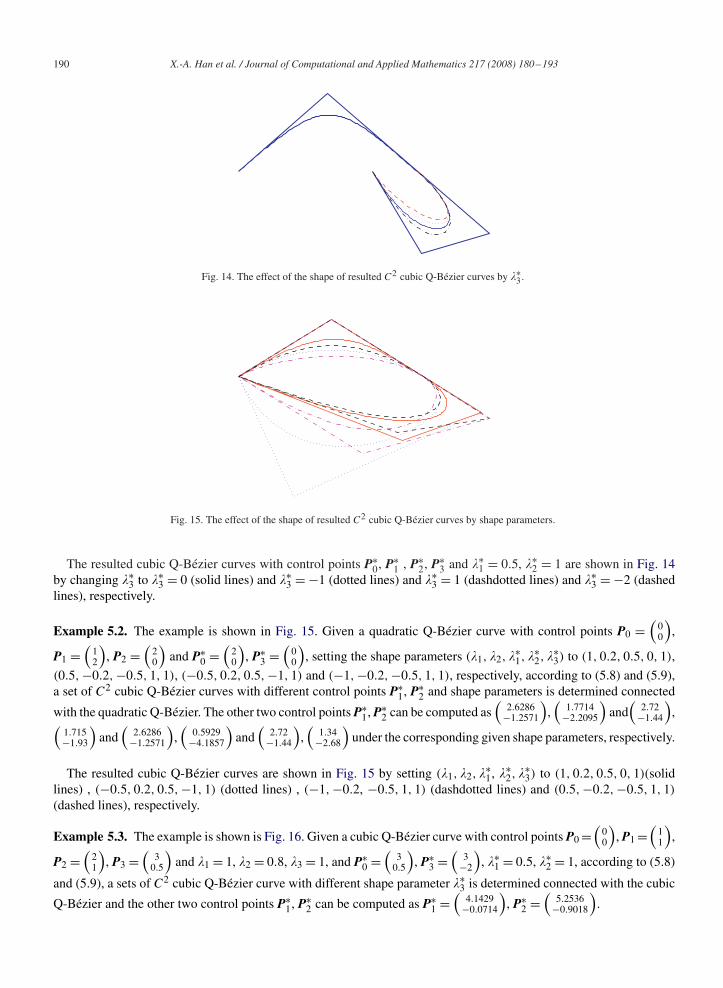
Fig. 15. The effect of the shape of resulted C2 cubic Q-Bézier curves by shape parameters.

The resulted cubic Q-Bézier curves with control points P∗0, P∗

1 , P∗2, P∗

3 and �∗1 = 0.5, �∗

2 = 1 are shown in Fig. 14by changing �∗

3 to �∗3 = 0 (solid lines) and �∗

3 = −1 (dotted lines) and �∗3 = 1 (dashdotted lines) and �∗

3 = −2 (dashedlines), respectively.

Example 5.2. The example is shown in Fig. 15. Given a quadratic Q-Bézier curve with control points P0 =(

00

),

P1 =(

12

), P2 =

(20

)and P∗

0 =(

20

), P∗

3 =(

00

), setting the shape parameters (�1, �2, �

∗1, �

∗2, �

∗3) to (1, 0.2, 0.5, 0, 1),

(0.5, −0.2, −0.5, 1, 1), (−0.5, 0.2, 0.5, −1, 1) and (−1, −0.2, −0.5, 1, 1), respectively, according to (5.8) and (5.9),a set of C2 cubic Q-Bézier curves with different control points P∗

1, P∗2 and shape parameters is determined connected

with the quadratic Q-Bézier. The other two control points P∗1, P∗

2 can be computed as(

2.6286−1.2571

),(

1.7714−2.2095

)and

(2.72

−1.44

),(

1.715−1.93

)and

(2.6286

−1.2571

),(

0.5929−4.1857

)and

(2.72

−1.44

),(

1.34−2.68

)under the corresponding given shape parameters, respectively.

The resulted cubic Q-Bézier curves are shown in Fig. 15 by setting (�1, �2, �∗1, �∗

2, �∗3) to (1, 0.2, 0.5, 0, 1)(solid

lines) , (−0.5, 0.2, 0.5, −1, 1) (dotted lines) , (−1, −0.2, −0.5, 1, 1) (dashdotted lines) and (0.5, −0.2, −0.5, 1, 1)

(dashed lines), respectively.

Example 5.3. The example is shown is Fig. 16. Given a cubic Q-Bézier curve with control points P0 =(

00

), P1 =

(11

),

P2 =(

21

), P3 =

(3

0.5

)and �1 = 1, �2 = 0.8, �3 = 1, and P∗

0 =(

30.5

), P∗

3 =(

3−2

), �∗

1 = 0.5, �∗2 = 1, according to (5.8)

and (5.9), a sets of C2 cubic Q-Bézier curve with different shape parameter �∗3 is determined connected with the cubic

Q-Bézier and the other two control points P∗1, P∗


(4.1429

−0.0714

), P∗

2 =(

5.2536−0.9018

).


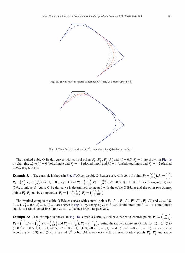
Fig. 16. The effect of the shape of resulted C2 cubic Q-Bézier curves by �∗3.

Fig. 17. The effect of the shape of C2 composite cubic Q-Bézier curves by �1.

The resulted cubic Q-Bézier curves with control points P∗0, P∗

1 , P∗2, P∗

3 and �∗1 = 0.5, �∗

2 = 1 are shown in Fig. 16by changing �∗

3 to �∗3 = 0 (solid lines) and �∗

3 = −1 (dotted lines) and �∗3 = 1 (dashdotted lines) and �∗

3 = −2 (dashedlines), respectively.

Example 5.4. The example is shown in Fig. 17. Given a cubic Q-Bézier curve with control points P0=(

0.20.5

), P1=

(11

),

P2 =(

21

), P3 =

(3

0.5

)and �2 =0.8, �3 =1, and P∗

0 =(

30.5

), P∗

3 =(

0.20.5

), �∗

1 =0.5, �∗2 =1, �∗

3 =1, according to (5.8) and

(5.9), a unique C2 cubic Q-Bézier curve is determined connected with the cubic Q-Bézier and the other two control

points P∗1, P∗


(4.1429

−0.0714

), P∗

2 =(

5.2536−0.9018

).

The resulted composite cubic Q-Bézier curves with control points P0, P1 , P2, P3, P∗0, P∗

1 , P∗2, P∗

3 and �2 = 0.8,�3 = 1, �∗

1 = 0.5, �∗2 = 1, �∗

3 = 1 are shown in Fig. 17 by changing �1 to �1 = 0 (solid lines) and �1 = −1 (dotted lines)and �1 = 1 (dashdotted lines) and �1 = −2 (dashed lines), respectively.

Example 5.5. The example is shown in Fig. 18. Given a cubic Q-Bézier curve with control points P0 =(

0−0.5

),

P1 =(

11

), P2 =

(31

), P3 =

(5

1.5

)and P∗

0 =(

51.5

), P∗

3 =(

3−1.5

), setting the shape parameters (�1, �2, �3, �

∗1, �

∗2, �

∗3) to

(1, 0.5, 0.2, 0.5, 1, 1), (1, −0.5, 0.2, 0, 0.2, 1), (1, 0, −0.2, 1, −1, 1) and (1, −1, −0.2, 1, −1, 1), respectively,according to (5.8) and (5.9), a sets of C2 cubic Q-Bézier curve with different control points P∗

1, P∗2 and shape


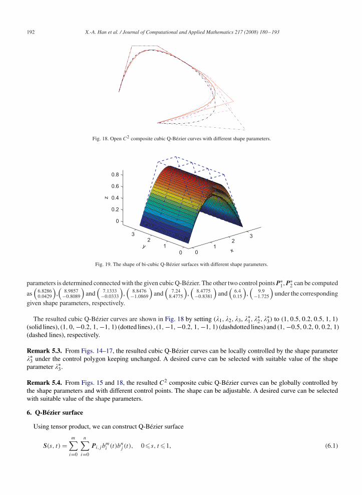
Fig. 18. Open C2 composite cubic Q-Bézier curves with different shape parameters.

01

23

0

12

3

0

0.2

0.4

0.6

0.8

xy

z

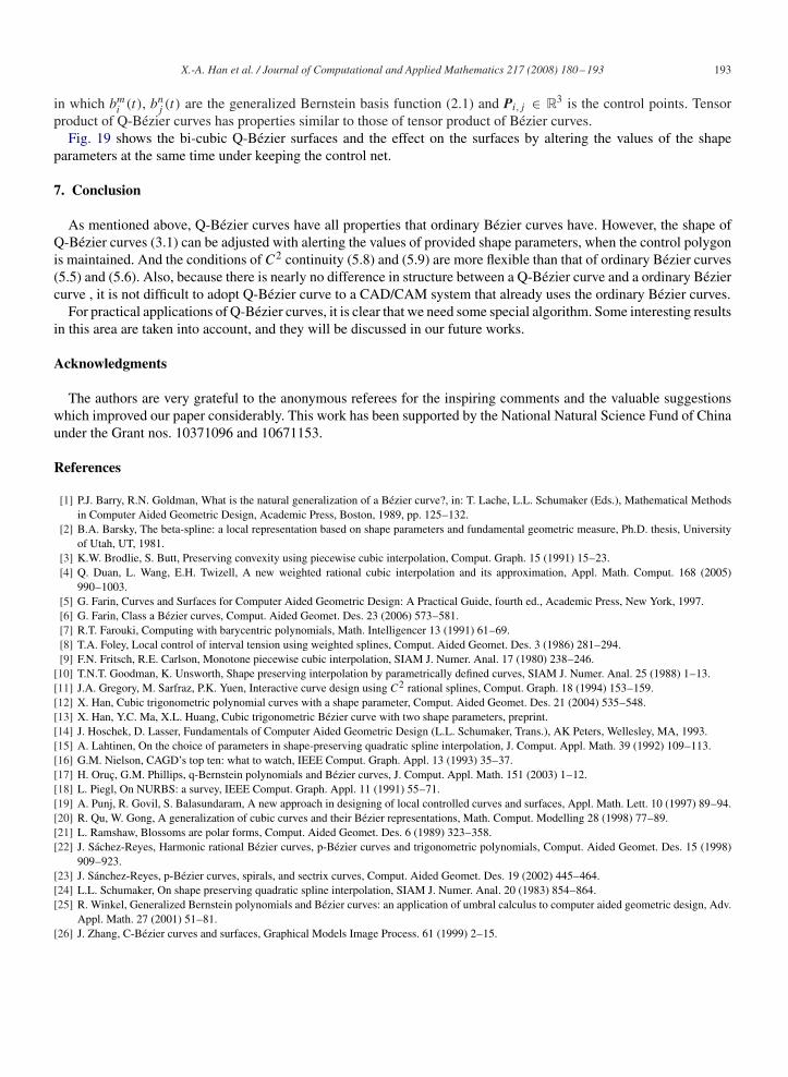
Fig. 19. The shape of bi-cubic Q-Bézier surfaces with different shape parameters.

parameters is determined connected with the given cubic Q-Bézier. The other two control points P∗1, P∗

2 can be computed

as(

6.82860.0429

),(

8.9857−0.8089

)and

(7.1333

−0.0333

),(

8.8476−1.0869

)and

(7.24

8.4775

),(

8.4775−0.8381

)and

(6.4

0.15

),(

9.9−1.725

)under the corresponding

given shape parameters, respectively.

The resulted cubic Q-Bézier curves are shown in Fig. 18 by setting (�1, �2, �3, �∗1, �

∗2, �

∗3) to (1, 0.5, 0.2, 0.5, 1, 1)

(solid lines), (1, 0, −0.2, 1, −1, 1) (dotted lines) , (1, −1, −0.2, 1, −1, 1) (dashdotted lines) and (1, −0.5, 0.2, 0, 0.2, 1)

(dashed lines), respectively.

Remark 5.3. From Figs. 14–17, the resulted cubic Q-Bézier curves can be locally controlled by the shape parameter�∗

3 under the control polygon keeping unchanged. A desired curve can be selected with suitable value of the shapeparameter �∗

3.

Remark 5.4. From Figs. 15 and 18, the resulted C2 composite cubic Q-Bézier curves can be globally controlled bythe shape parameters and with different control points. The shape can be adjustable. A desired curve can be selectedwith suitable value of the shape parameters.

6. Q-Bézier surface

Using tensor product, we can construct Q-Bézier surface

S(s, t) =m∑

i=0

n∑i=0

Pi,j bmi (t)bn

j (t), 0�s, t �1, (6.1)


in which bmi (t), bn

j (t) are the generalized Bernstein basis function (2.1) and Pi,j ∈ R3 is the control points. Tensorproduct of Q-Bézier curves has properties similar to those of tensor product of Bézier curves.

Fig. 19 shows the bi-cubic Q-Bézier surfaces and the effect on the surfaces by altering the values of the shapeparameters at the same time under keeping the control net.

7. Conclusion

As mentioned above, Q-Bézier curves have all properties that ordinary Bézier curves have. However, the shape ofQ-Bézier curves (3.1) can be adjusted with alerting the values of provided shape parameters, when the control polygonis maintained. And the conditions of C2 continuity (5.8) and (5.9) are more flexible than that of ordinary Bézier curves(5.5) and (5.6). Also, because there is nearly no difference in structure between a Q-Bézier curve and a ordinary Béziercurve , it is not difficult to adopt Q-Bézier curve to a CAD/CAM system that already uses the ordinary Bézier curves.

For practical applications of Q-Bézier curves, it is clear that we need some special algorithm. Some interesting resultsin this area are taken into account, and they will be discussed in our future works.

Acknowledgments

The authors are very grateful to the anonymous referees for the inspiring comments and the valuable suggestionswhich improved our paper considerably. This work has been supported by the National Natural Science Fund of Chinaunder the Grant nos. 10371096 and 10671153.

References

[1] P.J. Barry, R.N. Goldman, What is the natural generalization of a Bézier curve?, in: T. Lache, L.L. Schumaker (Eds.), Mathematical Methodsin Computer Aided Geometric Design, Academic Press, Boston, 1989, pp. 125–132.

[2] B.A. Barsky, The beta-spline: a local representation based on shape parameters and fundamental geometric measure, Ph.D. thesis, Universityof Utah, UT, 1981.

[3] K.W. Brodlie, S. Butt, Preserving convexity using piecewise cubic interpolation, Comput. Graph. 15 (1991) 15–23.[4] Q. Duan, L. Wang, E.H. Twizell, A new weighted rational cubic interpolation and its approximation, Appl. Math. Comput. 168 (2005)

990–1003.[5] G. Farin, Curves and Surfaces for Computer Aided Geometric Design: A Practical Guide, fourth ed., Academic Press, New York, 1997.[6] G. Farin, Class a Bézier curves, Comput. Aided Geomet. Des. 23 (2006) 573–581.[7] R.T. Farouki, Computing with barycentric polynomials, Math. Intelligencer 13 (1991) 61–69.[8] T.A. Foley, Local control of interval tension using weighted splines, Comput. Aided Geomet. Des. 3 (1986) 281–294.[9] F.N. Fritsch, R.E. Carlson, Monotone piecewise cubic interpolation, SIAM J. Numer. Anal. 17 (1980) 238–246.

[10] T.N.T. Goodman, K. Unsworth, Shape preserving interpolation by parametrically defined curves, SIAM J. Numer. Anal. 25 (1988) 1–13.[11] J.A. Gregory, M. Sarfraz, P.K. Yuen, Interactive curve design using C2 rational splines, Comput. Graph. 18 (1994) 153–159.[12] X. Han, Cubic trigonometric polynomial curves with a shape parameter, Comput. Aided Geomet. Des. 21 (2004) 535–548.[13] X. Han, Y.C. Ma, X.L. Huang, Cubic trigonometric Bézier curve with two shape parameters, preprint.[14] J. Hoschek, D. Lasser, Fundamentals of Computer Aided Geometric Design (L.L. Schumaker, Trans.), AK Peters, Wellesley, MA, 1993.[15] A. Lahtinen, On the choice of parameters in shape-preserving quadratic spline interpolation, J. Comput. Appl. Math. 39 (1992) 109–113.[16] G.M. Nielson, CAGD’s top ten: what to watch, IEEE Comput. Graph. Appl. 13 (1993) 35–37.[17] H. Oruç, G.M. Phillips, q-Bernstein polynomials and Bézier curves, J. Comput. Appl. Math. 151 (2003) 1–12.[18] L. Piegl, On NURBS: a survey, IEEE Comput. Graph. Appl. 11 (1991) 55–71.[19] A. Punj, R. Govil, S. Balasundaram, A new approach in designing of local controlled curves and surfaces, Appl. Math. Lett. 10 (1997) 89–94.[20] R. Qu, W. Gong, A generalization of cubic curves and their Bézier representations, Math. Comput. Modelling 28 (1998) 77–89.[21] L. Ramshaw, Blossoms are polar forms, Comput. Aided Geomet. Des. 6 (1989) 323–358.[22] J. Sáchez-Reyes, Harmonic rational Bézier curves, p-Bézier curves and trigonometric polynomials, Comput. Aided Geomet. Des. 15 (1998)

909–923.[23] J. Sánchez-Reyes, p-Bézier curves, spirals, and sectrix curves, Comput. Aided Geomet. Des. 19 (2002) 445–464.[24] L.L. Schumaker, On shape preserving quadratic spline interpolation, SIAM J. Numer. Anal. 20 (1983) 854–864.[25] R. Winkel, Generalized Bernstein polynomials and Bézier curves: an application of umbral calculus to computer aided geometric design, Adv.

Appl. Math. 27 (2001) 51–81.[26] J. Zhang, C-Bézier curves and surfaces, Graphical Models Image Process. 61 (1999) 2–15.

Documents

A novel generalization of Bézier curve and surface