OF UROFLOWMETRY CURVE SHAPES

STANDARDISED, AUTOMATIC DESCRIPTION

OF UROFLOWMETRY CURVE SHAPES

A thesis submitted in partial fulfillment of the requirements for the degree of Master of Science in Technical Medicine

Job S. de Haan

Faculty of Science and Technology, University of Twente

Department of Urology, University Medical Centre Utrecht

February 2020

Abstract

Rationale The shape of uroflowmetry curves might associate with voiding abnor-malities. The lack of standardisation in flow shape description impairs this diagnosticvalue and further research into shape descriptors. Therefore algorithmic analysis thatgenerates a complete shape description based on quantitative definitions for shapecharacteristics is proposed. A graphical user interface visually presenting the shapecharacteristics subject to the algorithmic evaluation makes this insightful for the end-user.

Methods Previously published quantitative definitions for flow shape are comple-mented with new proposals for standardised analysis when necessary. Objectivityin these proposals is improved by basing them on single center expert consensus.Urologists interpreted shape characteristics of sets of uroflowmetry curves together,resulting in a single assessment. Algorithmic performance and experience with theuser interface are improved by obtaining expert evaluation with goal oriented ques-tionnaires.

Results This resulted in an algorithm based on quantitative threshold evaluationfor a well-arranged set of shape characteristics. The generated description is com-prised of the descriptors bell shape, fluctuating, intermittent and plateau flow andcomments on symmetry and maximal flow. Deviation from threshold is made visiblein the uroflowmetry flow rate time graph for all shape characteristics. The user in-terface that makes the algorithm and the visualisation easily accessible is very wellreceived amongst the targeted users.

Conclusion Algorithmic description of uroflowmetry curve shape makes applica-tion of standardised evaluation fast and simple. The connected user interface providesvisual and textual substantiation for the generated description, encouraging the urol-ogist to be actively involved in shape evaluation. This evaluation method improvesthe diagnostic value of uroflowmetry and is ready for clinical implementation andintroduction elsewhere.

2

Graduation committee

Chairman / Technical supervisor:prof. dr. ir. B.J. GeurtsMultiscale Modeling and SimulationFaculty of Electrical Engineering, Mathematics & Computer ScienceUniversity of Twente, Enschede, The Netherlands

Medical supervisor:prof. dr. L.M.O. Heck – de KortDepartment of UrologyUniversity Medical Centre Utrecht, Utrecht, The Netherlands

Process supervisor:drs. R.J. HaarmanMaster’s programme Technical MedicineFaculty of Science and TechnologyUniversity of Twente, Enschede, The Netherlands

External member:dr. J. ZwiersCreative TechnologyFaculty of Electrical Engineering, Mathematics & Computer ScienceUniversity of Twente, Enschede, The Netherlands

ColloquiumFebruary 28, 202010:30 at TechMed Centre tl1133,University of Twente

3

Preface

This thesis is a product of the research I performed within the internship concludingthe technical medicine masters programme. In this research, I undertook thechallenge to automate a step in diagnosis that has no golden standard. My interestaroused during a short time internship on this subject a few months earlier. Ireturned to Utrecht motivated to make a meaningful contribution where technologyand clinical practice seemed to mismatch. Looking back on the past year, I amhappy to recognise that I have brought these two worlds closer together.

My enthusiasm was often fed by the two enthusiastic supervisors prof. de Kort andprof. Geurts. They have trusted me with much liberty in independently shapingand executing this research. Their appreciation of my work and support for furtherpossibilities motivated me to take it up a notch.

I would like to acknowledge all students that went before me and researched whatin hindsight proved to be more or less succesful approaches. This all has been avaluable reconnaissance paving parts of the road for me. For you are with many, Ithank Eliene, Mattiènne, Erik, Denise, Stef and Jeroen.

4

Contents

1 Introduction 61.1 Automating uroflowmetry curve shape assessment . . . . . . . . . . . . . . . . . . . . . . . . 61.2 Objectives . . . . . . . . . . . . . . . . . . . . . . . . . . . . . . . . . . . . . . . . . . . . . . 7

2 Background 82.1 Anatomy . . . . . . . . . . . . . . . . . . . . . . . . . . . . . . . . . . . . . . . . . . . . . . 82.2 Uroflowmetry . . . . . . . . . . . . . . . . . . . . . . . . . . . . . . . . . . . . . . . . . . . . 92.3 Previous research . . . . . . . . . . . . . . . . . . . . . . . . . . . . . . . . . . . . . . . . . . 11

3 Algorithm generation 133.1 Data acquisition . . . . . . . . . . . . . . . . . . . . . . . . . . . . . . . . . . . . . . . . . . 133.2 Set desired description . . . . . . . . . . . . . . . . . . . . . . . . . . . . . . . . . . . . . . . 133.3 Establish algorithm . . . . . . . . . . . . . . . . . . . . . . . . . . . . . . . . . . . . . . . . . 14

4 User interaction 194.1 Visualisation . . . . . . . . . . . . . . . . . . . . . . . . . . . . . . . . . . . . . . . . . . . . 194.2 Graphical user interface . . . . . . . . . . . . . . . . . . . . . . . . . . . . . . . . . . . . . . 234.3 Evaluation of usability . . . . . . . . . . . . . . . . . . . . . . . . . . . . . . . . . . . . . . . 23

5 Outlook and conclusions 265.1 Future recommendations . . . . . . . . . . . . . . . . . . . . . . . . . . . . . . . . . . . . . . 265.2 Conclusion . . . . . . . . . . . . . . . . . . . . . . . . . . . . . . . . . . . . . . . . . . . . . 27

References 28

Appendices 30

5

CHAPTER 1Introduction

1.1 Automating uroflowmetry curve shape assessmentUroflowmetry, the measurement of urine flow rate during urination, is widely used in diagnosis for patientswith lower urinary tract symptoms (luts). Apart from static parameters as voided volume and maximalflow, the shape of uroflowmetry curves might also associate with voiding abnormalities [1]. Assessment ofthe flow shape should therefore be part of evaluating the patient’s urination in diagnosis and/or evaluationof treatment efficacy [2]. It lacks standardisation when it comes to assessment of the flow shape, makingit susceptible to inter- and intra-observer variability. Algorithmic evaluation of curve shape characteristicsis proposed to ensure structured analysis based on standardised evaluations.

There are no concise guidelines for uroflowmetry curve shape assessment. A normal flow shape hasbeen defined as “arc-shaped with high maximum flowrate” by the International Continence Society (ics)but no quantitative range for this normal shape was provided. Furthermore, there is no standardisation indescribing abnormal flow shapes. This leaves assessment and description of flow shape to the individualurologist. Consequently, flow shapes are described inconsistently in literature. There is variability inquantitative definitions of the shapes, when presented, and in descriptors used for comparable flow shapes[2]. Recently, Netto et al. (2020)[3] have researched inter- and intra-observer variability in defining curveshape in a large, international scale study. They show how especially inter rater reliability is low andstretch how this makes shape definition unreliable for data analysis problems. A clear and consistentdescription is required to maximise diagnostic utility of uroflowmetry curve shape [4].

Li et al. (2018)[2] researched articles and ics standardisation documents for flow shape descriptorsused in literature. They recommended to use only “normal”, “fluctuating”, “intermittent”, and “plateau”descriptions with comment on symmetry and maximal flow. Fluctuating is describing an irregular curvewith multiple peaks. Intermittent is defined as flow stopping and starting during a single void. Plateau isa smooth, flat curve with lower flow rate and relatively longer flow time. Normal flow is an arc- or bellshaped curve without characteristics of these other flow shapes.

These flow shapes are carefully associated with underlying pathology. Flow curves described as fluc-tuating indicate detrusor-sphincter-dyssynergia. Intermittent flow relates to a poorly contractile detrusormuscle or voiding with abdominal straining. Plateau flow shapes indicate outflow obstruction or impaireddetrusor contractility. Uroflowmetry results are nowadays not specific for underlying causes so it shouldalways be interpreted together with examination and other adjunct investigations. However, when shapedefinitions are clearly defined and consistently applied, their association with underlying pathology can bethoroughly researched. [1, 5]

Standardised, quantitative definitions for the descriptors enable automated flow shape assessment.Advantageous is that this evaluation could be incorporated precisely in a computer algorithm. Automatedflow curve description is fast, easy and less prone to human errors. Consequently, its role in diagnosis willbe improved.

6

CHAPTER 1. INTRODUCTION

1.2 ObjectivesThe primary objective of the work reported in this thesis is algorithmic description of uroflowmetry curveshapes. This description should comprise the defining features of the curve shape. It is generated auto-matically based on quantitative definitions, therefore a complete set of parameters must feature what isdefining for the curve. The generated description is adequate and does not include an interpretation ofunderlying pathology.

Secondly, it is targeted to make the algorithmic generated description insightful for targeted users.For the algorithmic description to be endorsed and be adopted in clinical practice, the urologist shouldunderstand how evaluation resulted in the given description. This is done by visual representation of thequantitative definitions. Markers, lines etc. highlight (parameters representing) curve characteristics in theuroflowmetry graph. An easily accessible user interface makes switching between different visualisationspossible.

This thesis is structured as follows. Chapter 2 will walk through relevant background information,among which a short overview of important conclusions from previous attempts in taking on this challenge.After information about patient selection and the measurement device, in chapter 3 is worked on the firstobjective. It sets the desired output description and discusses considerations in all algorithmic evaluations.Chapter 4 is about the second objective, the users interaction with the algorithm. This comprises thevisualisation of shape characteristics, the final graphical user interface and results from its evaluation. Thelast chapter is devoted to concluding remarks and future recommendations.

7

CHAPTER 2Background

2.1 AnatomyContinuously production of urine in the kidneys fills the bladder via the ureters. The urinary bladder mustbe able to adapt in size to a socially adequate volume to store urine. The bladder wall is made up for themajority by muscle active in urination, the detrusor muscle. In total, the bladder is composed of smoothmuscle cells, collagen and elastin. The more collagen, the less compliant the bladder is. The bladderbody must contract simultaneously to achieve effective voiding. Micturition relies on detrusor contraction.Muscle energy is transferred into force (increase detrusor pressure) or muscle shortening (decrease bladdervolume) depending on outflow resistance. The latter leads to flow of urine. [6, 7]

Because of characteristic properties of muscle tissue, urine flow is dependent on bladder volume. Thelength for the muscle fibres at which potential bladder power is largest is usually reached at volumesof 150-250 ml. For volumes higher than 400-500 ml the muscles can become overstretched, decreasingcontraction power. [1]

Figure 2.1: Anatomy of the bladder and urethral sphincters in A) women and B) men. Reprinted from [8].

At the bottom a funnel shaped extension of the bladder, the bladder neck, connects with the urethra(see Figure 2.1). The urethra is composed of striated and smooth muscles and is important in maintainingcontinence. Maintaining continence is a combination of active muscle tone and passive anatomic coaptation.The muscle structures aid in occlusion of the urethral muscles but as well in opening of the bladder neckduring micturition.

8

CHAPTER 2. BACKGROUND

There is more than one structure that acts as sphincter. Their distinction remains somewhat un-clear and differs between genders. In women (Figure 2.1 A), muscle cells that extend from the proximalurethra distally form the internal sphincter. This internal smooth muscle sphincter is horseshoe-shaped.The external sphincter or rhabdosphincter consists of striated muscle in the urethra wall that graduallyincreases until the level of the periurethral muscles of the pelvic floor. During bladder filling the sphinctersincrease pressure along their circumference to maintain continence. Additional muscle structures are calledcompressor urethrae and urethrovaginal sphincter. In men (Figure 2.1 B), the internal sphincter locatesbetween the bladder and the prostate. The rhabdosphincter configures near the prostatic apex. Mengenerally have a higher outflow resistance because of their longer urethra and the (with age increasing)obstructive effects of the prostate. [6, 7]

InnervationThe lower urinary tract receives parasympathetic, sympathetic and somatic innervation. Parasympatheticnerves that arise at sacral level excite the bladder and relax the urethra. Sympathetic nerves from spinalcord levels T10-L2 inhibit the bladder body but excite bladder neck and urethra (internal sphincter). Theexternal urethral sphincter is excited by the somatic nervous system (spinal cord levels S2-4) and thereforeunder voluntary control. Thus, the storage phase of the bladder can be switched to the voiding phaseeither reflexively or voluntarily. Involuntary voiding occurs for example in children and patients withneuropathic bladder. [6, 7]

2.2 UroflowmetryBecause it is both non-invasive and inexpensive, uroflowmetry is an accessible first-line screening testto provide objective and quantitative information about both storage and voiding function [1]. Thisinformation has diagnostic value and can indicate additional diagnostic tests. It also serves as a methodfor evaluation of therapy in follow-up. The first uroflowmeter was invented by Willard M. Drake Jr. in1946 under the name “pissometer”, see Figure 2.2. The main structure was a balance with a container onone arm and a spring and pen on the other arm. Because of the increasing weight caused by urinating inthe container the balance shifts and the other arm moves proportionally to the increase in voided volume.This is registered since the pen mounted to that arm writes on a kymograph. [9]

Figure 2.2: Design for first uroflowmeter by Willard M. Drake Jr. in 1946. From left to right the separate partsare a kymograph, a spring loaded balance with a writing arm, a fluid container and a collection funnel. Adaptedfrom Chancellor (1998) [9].

In time, uroflowmetry devices were improved. Nowadays, there are various systems with differencesin appearance and underlying technology. This study remains limited to free flow uroflowmetry, voidingwithout restriction or alteration by a bladder catheter or such. The weight transducer is most popular.

9


Its mechanism is most similar to Drake’s device since flow is derived from mass of voided volume. Becauseof the force the increasing weight of urine exerts on the measurement device, a strain gauge load celldeforms appropriately. The electrical resistance changes proportionally to weight causing deformationso electrical currents measured can be calibrated for voided volumes. Two other popular mechanismsare dipstick and rotating disc. A dipstick in uroflowmetry is a capacitor vertically placed in the urinecollection reservoir. The height to which it is submerged in fluid, affected by the solutes in urine, changesthe electrical capacitance of the dipstick. This allows for similar calibration as for the weight cell. Arotating disc measures the power necessary to maintain a constant rotation speed. Urine landing on thedisc slows the disc down so measurable additional power from the rotation motor reflects the urine flowrate. [10, 11]

When working with uroflowmetry, certain restrictions of the measuring technique must be taken intoaccount. For example the voiding may be influenced by a set of external factors. Therefore the patientshould void when they feel what they personally recognise as a normal desire to do so. Afterwards, thepatient should be asked if the current voiding was representative for their usual voiding. There are technicalrestrictions as well. The largest follow from the set-up. Due to physics, urine breaks into drops outside theurethra. This creates irrelevant high frequencies in the recording. Secondly, the funnel shaped recordingdevice also causes modifications to the recording because it introduces a delay that is subject to where inthe funnel the urine stream lands. [1]

Test resultRegardless of the type of uroflowmeter, result of the test is a registration of the amount urine over thetime in which it is voided. Flow rate is the rate of volume change over time. The time derivative is acalculation and is therefore an indirect test result. Visual presentation is a graph of voided volume and/orflow rate against time. The latter (see Figure 2.3) is subject of this research. Conventional units aremillilitres per second for flow rate and seconds for voiding time. Precision and smoothness of the curve arepredominantly determined by sample rate and signal processing. The ics recommends a sample rate of 10Hz to deal with unwanted high frequencies and a moving average with two seconds window to minimizethe funnel effects [1]. Major measurement parameters are maximal and average flow rate, voided volume,flow time and time to maximum flow as standardised by the ics [10]. These are visualised in Figure 2.3.

Figure 2.3: Example of an uroflow curve with parameters Qmax (maximal flow rate); Vvoid (voided volume);Qave (average flow rate); flow time, time to void in seconds; time to Qmax; time to reach Qmax in seconds.Reprinted from Chun et al. (2017) [10].

Urine flow rate measurements are influenced by detrusor contractility (neurogenic and myogenic),outflow resistance and bladder volume. Normal urine flow results in a bell-shaped curve. Reduced flowor an altered pattern could indicate underactive bladder or bladder outlet obstruction. An interrupted

10


or straining pattern can be seen with impaired detrusor contractility, obstruction or voiding with abdom-inal straining. Notice all the careful formulations within these sentences since precise interpretation isyet only possible when flow rate is compared to simultaneously recorded pressure recordings in invasiveurodynamics. [6, 1]

2.3 Previous researchWithin a collaboration between University Medical Centre Utrecht (umcu) and University of Twente (ut),the first step in algorithmic evaluation of uroflowmetry curves was made in 2014. Since then a series of sevenstudent internships contributed directly to this project. This section will provide important considerationsfollowing from these internships, that are taken into account in order to reach the objective.

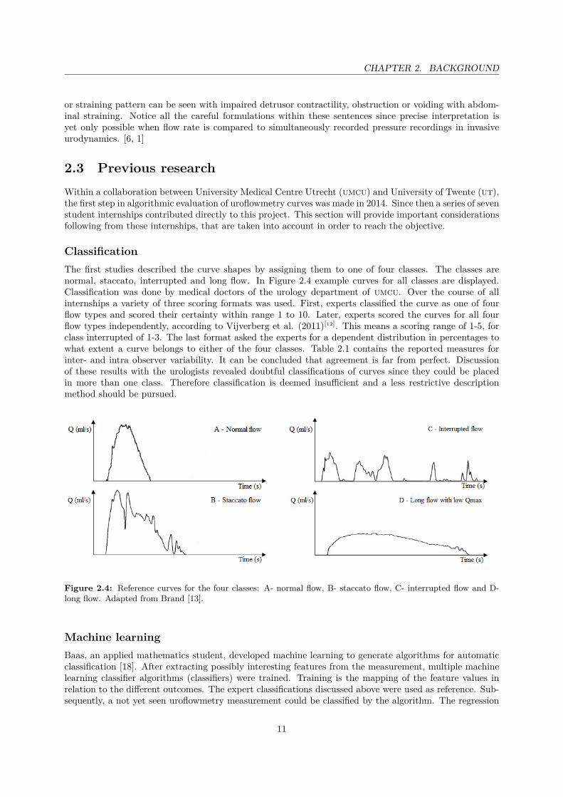
ClassificationThe first studies described the curve shapes by assigning them to one of four classes. The classes arenormal, staccato, interrupted and long flow. In Figure 2.4 example curves for all classes are displayed.Classification was done by medical doctors of the urology department of umcu. Over the course of allinternships a variety of three scoring formats was used. First, experts classified the curve as one of fourflow types and scored their certainty within range 1 to 10. Later, experts scored the curves for all fourflow types independently, according to Vijverberg et al. (2011)[12]. This means a scoring range of 1-5, forclass interrupted of 1-3. The last format asked the experts for a dependent distribution in percentages towhat extent a curve belongs to either of the four classes. Table 2.1 contains the reported measures forinter- and intra observer variability. It can be concluded that agreement is far from perfect. Discussionof these results with the urologists revealed doubtful classifications of curves since they could be placedin more than one class. Therefore classification is deemed insufficient and a less restrictive descriptionmethod should be pursued.

Figure 2.4: Reference curves for the four classes: A- normal flow, B- staccato flow, C- interrupted flow and D-long flow. Adapted from Brand [13].

Machine learningBaas, an applied mathematics student, developed machine learning to generate algorithms for automaticclassification [18]. After extracting possibly interesting features from the measurement, multiple machinelearning classifier algorithms (classifiers) were trained. Training is the mapping of the feature values inrelation to the different outcomes. The expert classifications discussed above were used as reference. Sub-sequently, a not yet seen uroflowmetry measurement could be classified by the algorithm. The regression

11


Table 2.1: Reported inter- and intra observer variability measures for different data sets and scoring methods.Kappa level of agreement is classified according to Landis et al. [14]. auc mae is area under the curve of the meanabsolute error plot. * 1: one of four classes, 2: independent scores Vijverberg[12] 3: percentage distribution. **Different number of experts scored three datasets, results are averages weighted for database size.

Researcher (no. of curves)

{scoring method*}

No. of

expertsKappa

Kappa level of

agreement

AUC

MAE

Level of

agreement

Inter observer variability

Kamp, van der [15] (665) {1} 3 0.58 Moderate 0.82 -

Brand [13] (90) {1} 3 0.34 Fair - -

Boele [16] (84) {2} 3-5** 0.36 Fair 0.69 59 %

Haan, de [17] (100) {3} 4 - - 0.84 37 %

Intra observer variability

Kamp, van der [15] (100) {1} 3 0.86 Almost perfect - -

Brand [13] (10) {1} 3 - - - 87 %

Boele [16] (18) {2} 3-5** 0.73 Substantial - 79 %

Haan, de [17] (17) {3} 4 - - 0.90 70 %

forest classifier yielded the best results with an estimated accuracy of 97% on new measurements [18]. Thisshowed a classifier could be trained well on a dataset of fixed expert reference classifications.

In the process of clinical validation was found that the reported accuracy of the machine learningclassifier was overestimated. The algorithm lost accuracy when compared to expert classifications of newmeasurements. This is attributed to the subjective nature of these classifications. All disadvantages fromthe lack in consistency in the expert reference scoring apply here as well. The classifiers are inherentlydependent on the expert reference scoring since they must learn from example classifications. [17]

Component based analysisValidation of the machine learning classifier pointed out that automatic classification of the curve willnot be fully endorsed when it works as a black box and provides its own conclusion that is not alwaysaccurate. Algorithmic evaluation of curves will probably be best accepted when it provides insight inhow the conclusion was formed. It should improve objectivity and consensus between experts when itintelligently evaluates essential characteristics of the curve and in that way draws attention to the importantinformation and presents this in a coherent way.

In one of the later internships, Haaren explored component-based analysis of uroflowmetry curves thatprovides insight in the analysis [19]. It allowed multiple descriptors to be applied to a single curve basedon simple threshold evaluations. Furthermore it used visual indicators for the different parameters andtheir corresponding thresholds. This attempt proved to be very valuable since it removed dependabilityon training data subject to variance and connected well with clinicians wish to better understand theprocess of automatic curve description. Thresholds were, however, not very well substantiated and thepresentation of information was quite overwhelming. Due to the promising results and clear starting pointsfor improvement this direction was continued in the current research.

12

CHAPTER 3Algorithm generation

3.1 Data acquisitionUroflowmetry measurements used in this study are recent measurements of patients with lut dysfunctionsymptoms from the urology outpatient clinic of umcu. Patients are of both genders, aged 18 and up. Alluroflowmetry measurements in the period from early July to mid-September 2019 are obtained, there is noselection on symptoms or diagnosis in hindsight. Data is fully anonymous except for gender. All patientsare over 18 years old, measurements with a voided volume below 100 ml were excluded. This resulted in219 uroflowmetry measurements available for evaluation. Of these measurements 145 (66%) were of malepatients.

Uroflowmetry was done when patients felt normal desire to void. They were instructed to void like theynormally would on a regular toilet, in a position of their preference. No additional action was requiredof the patients and measurements cannot be traced back to individual persons. The medical researchethical committee metc Utrecht ruled therefore that this research is not subject to the Medical ResearchInvolving Human Subjects Act (wmo).

Measurements are performed on the FlowClean uroflowtoilet (Urotex, The Netherlands), a weighttransducer uroflowmeter. The device has a sample rate of 10 Hz, device software filters the signals witha moving average filter with window length of one second. This window length is shorter than the twoseconds as recommended by the ics.

3.2 Set desired descriptionLi et. al. (2018)[2] did a proposal for flow shape description in conclusion of their review article. Quote:“We suggest that only ’normal’, ’fluctuating’, ’intermittent’, and ’plateau’ descriptions, with additionalcomment on symmetry and qmax, be used to describe urine flow rate curve shape, and the definitions forthese descriptors should follow the terms in the ics standardisation documents [2].” These descriptors referto actual shape and are more easily defined than descriptions of the presumed cause of the shape. In thecurrent research was chosen to stay close to this proposition. However, ’bell shaped’ will be used insteadof ’normal’. Normal urine flow results in a bell shaped curve, the latter being a shape descriptor instead ofa diagnostic interpretation. Therefore it fits better with the goal of shape description and among the otherdescriptors. Comment on symmetry and qmax (maximal flow rate) was not further defined in the proposal.In the current research is chosen for simple, not quantitative commentary on these characteristics. Whenmaximal flow is considerably higher or lower than reference value this will be mentioned. Symmetry willbe categorically distinguished between asymmetrical and fairly symmetrical.

The description described above is additional to essential information that uroflowmetry currentlyalready presents. The graph depicting urine flow rate over time and standard parameters should remainwithin the test output. Most important parameters are qmax, voided volume and total flow time. Asstandardised in the ics technical report, uroflowmetry documentation should contain information in a

13

CHAPTER 3. ALGORITHM GENERATION

certain format [1]. This format is void = Maximum Flow Rate/Volume Voided/Post Void ResidualVolume. Therefore this was made part of the description except for residual bladder volume since it doesnot follow from the time/flow rate relationship.

3.3 Establish algorithmIn the algorithm all steps towards the desired description above are automated. Input is just the timeand flow rate vector of the uroflowmetry measurement and the gender of the patient. To algorithmicallyevaluate applicability of the descriptors, quantitative components must be found for discriminating charac-teristics corresponding to those descriptors. The review by Li provides some parameters with quantitativethresholds. When sufficient and unambiguous these are adapted in the algorithm. However often direc-tives for the curve shape descriptors were incomplete or contradict each other. Steps undertaken to cometo a applicable evaluation are described below. Multiple times will be referred to a consensus meeting.This means that the challenge in question is discussed in a meeting with three to five medical doctorsof the urology department of umcu under supervision of the researcher. These doctors are tasked withinterpretation of uroflowmetry measurements in their day to day work. Multiple uroflowmetry curves arediscussed then with output (classification, selection of timestamps) depending on the question. In this wayobserver variability is of far less influence. Curve parameter thresholds referred to in text are accumulatedin Table 3.1.

Start and stop of voidingThe initial step is assuring that the measurement data is fit for automatic analysis. While evaluatingperformance of algorithmic evaluation presented in previous research was found that often the time vectorof the measurement is considerably longer than what urologists describe as relevant voiding. As will beseen, the majority of evaluated parameters is time dependent. Therefore correct definition of start andend of relevant voiding are important for the correct description. These points were not clearly definedbefore [2]. Together with technical medicine intern S. Pham work was done on adequate detection ofrelevant flow. His report reflects on four different algorithms [20]. These algorithms were compared withexpert defined endpoints in the consensus meeting. Based on this information a combination of a flow-and volume threshold for evaluation of start and stop of voiding were applied in the description algorithmof the current study. As will be explained this evaluation has multiple applications.

Very low flow is not regarded as relevant flow. Therefore flow below the threshold of 0.5 ml/s is seenas no voiding in analysis. When flow rate crosses the threshold value this marks the start or stop of flow.Parts of flow are consequently defined from the first to last joined value above threshold. In interruptedflows, the flow rate rises again after it dropped below the threshold. These parts might be relevant sinceintermittent voiding is one of the characteristic flow shapes. To distinguish between intermittent voidingand eventual dribbling exceeding the flow threshold, the volume threshold was applied. A part of flowis deemed relevant when the volume voided in that part is at least 5 ml. Voided volume is equal to thearea under the curve, approached by integration with matlab (version 2018b, Mathworks, usa) builtin function trapz. When a flow curve consist of two of more relevant flow parts and thus at least aninterruption the descriptor intermittent is applicable [2].

Previous research proposed 0.2 ml/s and 5 ml for flow- and volume threshold respectively [15]. Phamproposed the thresholds 1 ml/s and 2 ml based on a droplet simulation experiment, but due to a combi-nation of limitations of this approach was not chosen to substitute the thresholds for these values. Theflow threshold was increased to 0.5 ml/s in consultation with the urologists in Utrecht and according tothe more recent proposal from a study by Gammie et al. (2016)[21]. For threshold 0.2 ml/s sometimesa for the eye evidently intermittent curve was described as fluctuating because the interruption was notrecognised.

Another product of this evaluation is the main flow part. In flows that are intermittent, the mainflow part is the part with the largest voided volume. In this study that always corresponds to the part inwhich qmax is found. Evaluation of the rest of the flow part characteristics will concentrate on the mainpart. With the notion that these curves are intermittent, analysis of the main flow part provides most

14


additional information about the time volume relationship while voiding. Figure 3.1 shows the differencesbetween original flow, relevant flow and main flow part for an example flow curve.

Figure 3.1: This line represents the complete flow time graph resulting from uroflowmetry in a single patient.The part that is black is deemed irrelevant because flow does not exceed 0.5 ml/s and when it does the volumeexcreted is less than 5 ml. As a result only the blue part of the curve is shown and used for analysis. The remainderis separated by flow (almost) reaching baseline. Of these three parts the first corresponds to the largest volumeexcreted and is considered the main flow part.

FluctuationsThe review by Li et al. presents three quantitative thresholds. Equal to the square root of qmax inml/s, to 20% of qmax in ml/s and 5 ml/s [2]. A sub-study comparison of these thresholds was executed(Appendix iv). Mutual differences were investigated and the outcome per threshold was compared withexpert classification yielded in a consensus meeting. This resulted in selection of threshold 20% of qmax(ml/s).

Fluctuations were identified by detection of their peaks. Peak detection was executed with the matlabbuilt in function findpeaks. This function finds local maxima by comparing sample values with adjacentvalues. To limit detected peaks to only the ones exceeding the threshold, the setting MinPeakProminencewas used. The drop in signal value on either side before the signal attains a higher value is calculated.The smallest of the two is the prominence of that peak. Peak detection is limited to peaks where theprominence is at least 20% of qmax.

Due to the calculation of prominence, two very close local maxima with the exact same flow rate areboth detected as peak. They are however part of the same peak. The function has two output arguments:peak values and their corresponding instances. When two succeeding peaks have the same value and arewithin one second from each other, the second peak is deleted.

The ics defines fluctuating flow as ’multiple peaks during a period of continuous urine flow’ [22].Therefore, peak detection is applied only to the main flow part in interrupted flow measurements. Theamount of fluctuations is the number of peaks exceeding threshold value additional to the peak corre-sponding to qmax. The peak corresponding with the maximal flow is also detected but this is not labelledas fluctuation. Therefore the vector with peak instances is compared to the instance of qmax resulting inthe deletion of this point. If there is one or more fluctuations, the curve is described as fluctuating.

PlateauFor the plateau descriptor multiple definitions are defined. Taken together, plateau curves have relativelylonger flow time and are flattened with a constant qmax very close to the average flow. More specific,quantitative definitions are aimed at different aspects of this description. The flattened shape with high

15


average flow results in a high ratio of average flow to maximal flow (qr (1)). As threshold for plateau, thisratio should be at least 0.8 [23]. The relative length of flow time is represented in parameter tq (s2/ml),the ratio of voiding time to qmax. A plateau defined by a flattened shape with constant qmax is restrictedto variations less than 1 ml/s for at least 4 seconds [24, 25]. In case of a high qr, the plateau characteristicis most complete since in these curves the maximal flow is most evidently restricted. However, with thecurrently aimed at shape description, different shape characteristics may be applicable for the same curve.When the plateau characteristic is present but not reflected in the entire duration of the measurement theqr threshold is hard to be met. The other definitions are combined to also selectively recognise flow curveswith a shorter plateau. When a plateau is present (variations >1 ml/s for at least 4 seconds) and thevoiding time is relatively long (tq > 2 s2/ml [26]) the curve is also described as plateau flow. Essentialrequirement is that the point of qmax lies within this interval otherwise the plateau does not represent aflattened curve.

Bell shapeNormal flow has been described accordingly in most articles. Definitions are bell shaped, approximatelysymmetrical, uninterrupted and without rapid amplitude changes [2]. Because all other characteristics aretreated separately, now will be focussed on the bell shape. For this shape different thresholds are usedfor the parameters qr and tq. Characteristic for bell shaped curves is qr higher than 0.63 and tq lowerthan 1.28 s2/ml [27]. A third relevant parameter is the ratio of time after qmax to time before qmax(dtat (1)). Reported threshold values for bell shape; 0.85 < dtat < 2.12 [27] and 2.33 [28], are nowcombined in 0.85 < dtat < 2.33. Nishimoto et al. (1994)[27] are the only ones reporting a combinationof three parameters. Other articles in the Li review used shape characteristics analogous to one or two ofthese three requirements. Therefore in this research a flow curve is described as bell shaped when two ofthese three parameters are within threshold limits. The conditions for plateau and bell shape flow are notautomatically mutually exclusive. However, in perception, the presence of a plateau cannot coexist witha bell shaped pattern. Therefore, in the algorithm evaluation for the plateau descriptor happens first andwhen it is applicable this prevents the curve from being described as bell shaped.

Maximal flowMaximum and average flow rates are related to volume. Research towards this relationship has resulted inmultiple nomograms for either voided volume or bladder volume. These provide insight in normal limitsfor maximal flow rate, aiding in clinical interpretation of uroflowmetry. There is no standardised preferencefor a single nomogram. For adaptation in the current algorithm was chosen for the Liverpool nomogramsby Haylen et al. (1989)[29]. That study produced nomograms for a wide range of voided volume formen/women separately. Voided volume is a direct result of uroflowmetry and using this does not requireseparate measurement of residual bladder volume. The wide range of flows for both genders makes thenomogram most suitable to the wide variety of the algorithm’s target population. The nomograms forwomen and men can be seen in Figure 3.2. The equations of these graphs (50th percentiles) were suppliedin the original article [29] and are implemented in the algorithm.

When the maximum flow rate of a flow curve is close to the reference maximum corresponding withthe voided volume, the description is not altered. When it is substantially higher or lower it is referredto in the description. Boundaries for substantial are the 25th an 75th percentile graphs of the nomogram(see Figure 3.2 A and B). For these graphs representing the percentile lines no equations were supplied.Boundaries are therefore based on the deviation of the graphs in respect to the 50th percentile graph.This deviation of the 25th an 75th percentile was approached by 4 ml/s at 100 ml voided volume linearlyincreasing to 6 ml/s for men and to 10 ml/s for women at 600 ml. The nomogram can not be extrapolatedfor volumes higher than 600 ml because it can not be assumed that the corresponding maximum flowkeeps increasing as well. At a certain point flow rate will be restricted by anatomical structures insteadof bladder volume. Therefore values in measurements with voided volume over 600 ml will be comparedwith reference values corresponding to 600 ml voided volume. Volumes below 100 ml voided volume donot occur due to inclusion criteria.

16


Figure 3.2: Liverpool nomograms for maximum urine flow rate. A) In women, B) In men under 50 years (medianage 35). Dotted lines represent the 5th, 10th etc. percentile. Reprinted from Haylen et al. (1989) [29].

SymmetryIn Li’s review article, comment on symmetry was suggested as additional part of uroflowmetry shapeevaluation [2]. No strong substantiation for describing this characteristic was provided in that or otherarticles. The review points out how it provides nuance among the four descriptors, preventing the needfor extra descriptors. For example the descriptor “compressive” should not be used since it implies acause. This shape can now be described as asymmetric flow with low maximum flow. Just like the otherdescriptors, additional diagnostic value of reporting symmetry can be retrospectively evaluated whencompared to additional diagnostic tests. There is no precedent in systematically determining symmetryof uroflowmetry curves. The aim is evaluating symmetry with respect to a vertical symmetry axis. A flowshape would be perfectly symmetric when this axes is at the point of qmax with equal curve slope oneither side. Symmetry is mentioned as characteristic of bell shaped curves. Of parameters related to thisdescriptor, dtat is best in comparing the slope before and after maximum flow. Experimenting with thisparameter for symmetry pointed out that it is too dependent on the time stamp of qmax. When qmaxis for example caused by a fluctuation or is in reality not very restricted to that single point in case of aplateau, dtat did not successfully represent symmetry.

A more successful way of comparing how flow rate increases and decreases was implemented from theinternship of E. Biel [30]. This student researched new parameters of uroflowmetry curves among whichthe maximal and minimal slope of the curve. These were calculated as tangents to a smoothed versionof the curve achieved by curve fitting. According to that study a fourth order polynomial fit and a 0.10Hz low-pass Butterworth filter performed best. In consultation with Biel was expressed that the latterwas likely to perform best when applied to a wider variety of uroflowmetry shapes because of inherentproperties of the polynomial fit. As measure for symmetry is chosen for the point where the maximal andminimal slope tangents intersect. An example of a fitted curve with its tangents can be seen in Figure 4.3D. The parameter sip is the intersection time normalised by dividing it by the total voiding time. A rangefor this parameter that corresponds to symmetric curves was set with aid of another consensus meeting.A team of three physicians classified 40 curves as ‘asymmetrical’ or ‘fairly symmetrical’ unanimously. Ofthis set 17 curves were classified fairly symmetrical, sip 0.21 ± 0.07 (median ± standard deviation). Theremaining 23 asymmetrical curves had sip value 0.09 ± 0.06. Threshold optimization was done to bestmatch algorithmic classification to this consensus classification. This way a lower bound of sip = 0.15 wasfound. No curve was classified as asymmetrical with a high sip value. What follows from the range fordtat in bell shape definition (0.85-2.33), is that skewness to the left is anticipated more than skewness tothe right. Therefore the upper bound for sip was now carefully set at 0.6.

17


Table 3.1: Overview for parameter thresholds. Thresholds marked with ‘*’ are part of simultaneous evaluationof multiple parameters, see text for details.

Parameter Description Thresholds

interruptions Number interruptions between partsof flow

Intermittent; interruptions > 0,

Flow rate threshold part of flow = 0.5 ml/s,

Volume threshold part of flow = 5 ml

fluctuations Number of fluctuations in flow rateabove threshold

Fluctuating; fluctuations > 0,

Fluctuation threshold = 0.2 × Qmax (ml/s)

Qr Ratio of average flow rate to maximalflow rate

Plateau; Qr > 0.8

Bell shape; Qr > 0.63*

TQ Ratio of voiding time to maximal flowrate

Plateau; TQ > 2 s2/ml*

Bell shape; TQ < 1.28 s2/ml*

plateau Duration of constant flow with no fluc-tuations above threshold

Plateau; plateau > 4 s*,

Fluctuation threshold = 1 ml/s

DTAT Ratio of time after maximal flow totime before maximal flow

Bell shape; 0.85 < DTAT < 2.33*

Qmax Maximal flow rate Low/ high Qmax outside first and third quartileof Liverpool nomograms

SIP Symmetry intersection point of tan-gents to fitted curve

Fairly symmetric 0.15 < SIP < 0.6

18

CHAPTER 4User interaction

4.1 VisualisationThis section focusses on considerations in presenting data for end users. First there is attention forpresentation of the standard parameters and the time flow rate graph. Then will be addressed howadditional parameters and the algorithmic description are made insightful. This generally consists of avisual and a textual component. Relevant characteristics of the time flow rate graph are highlighted andsupporting text or additional parameters are presented.

Original uroflowmetryThe ics technical report recommended the following standards for the time flow rate graph: a range of0-50 ml/s for flow rate and that 1 ml/s on the y-axis corresponds to 1 ml on the x-axis. Additionally itcontains recommendations on the presentation and documentation of some parameters. Considering thetechnical accuracy of uroflowmetry, flow rate (ml/s) should be rounded to integers. Voided volume shouldbe rounded to nearest plural of 10 ml. [1]

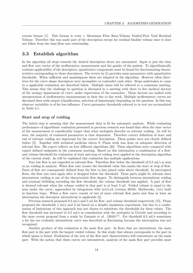
Reference curve and maximal flowTo present context for the shape of the uroflowmetry curve, a reference curve is plotted together with thetime flow rate graph. This reference curve is based on the bell shape corresponding to normal voidingadapted to the current measurement. Starting point to make it measurement specific is the relationshipbetween maximal flow rate and voided volume of the Liverpool nomograms. For the specific void andpatient gender the resulting maximal flow is set as tip of the reference curve. The curve itself is based onthe generic formula for statistic normal distribution since this is a bell shape as well. A slight adjustmentwas made to delete the lowest part of this distribution since it is to flat for a uroflowmetry measurement.The value that normally represents the standard deviation an influences the width of the graph wasempirically adjusted so that the area under the reference curve (equal to volume) is about equal to thevoided volume of the measurement. This value scales with voided volume. The specific creation of thisreference curve with the adjusted formula can be found in Appendix iii. The result can be seen in Figure4.1. This figure additionally shows how high or low maximal flow in the description is made insightful.Horizontal lines above and below the reference curve qmax show boundaries for this evaluation.

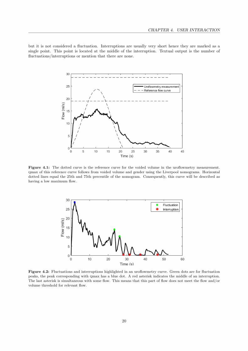
Fluctuations and interruptionsProviding insight in the descriptors fluctuating and intermittent is straightforward. The applicability ofthese descriptors follows directly from the presence of respectively fluctuations and interruptions. Sub-stantiation consists of pointing out this presence. In Figure 4.2 can be seen how detected fluctuationsand interruptions are emphasized. Fluctuation indicators are placed on detected peaks above fluctua-tion threshold. The peak corresponding with qmax is a different color since it is a peak above threshold

19

CHAPTER 4. USER INTERACTION

but it is not considered a fluctuation. Interruptions are usually very short hence they are marked as asingle point. This point is located at the middle of the interruption. Textual output is the number offluctuations/interruptions or mention that there are none.

Figure 4.1: The dotted curve is the reference curve for the voided volume in the uroflowmetry measurement.qmax of this reference curve follows from voided volume and gender using the Liverpool nomograms. Horizontaldotted lines equal the 25th and 75th percentile of the nomogram. Consequently, this curve will be described ashaving a low maximum flow.

Figure 4.2: Fluctuations and interruptions highlighted in an uroflowmetry curve. Green dots are for fluctuationpeaks, the peak corresponding with qmax has a blue dot. A red asterisk indicates the middle of an interruption.The last asterisk is simultaneous with some flow. This means that this part of flow does not meet the flow and/orvolume threshold for relevant flow.

20


Additional parametersThe additional parameters qr, tq and dtat are of relevance for the descriptor bell shape and, except forthe latter, for the descriptor plateau. Values for these parameters are presented when these descriptors areconsidered. Here, visualisation aims at showing how the parameters are calculated and how they relate tothreshold values. To keep the imagery clear, these visualisations are only shown when parameter valuesare deviating. The results can be seen in Figure 4.3 A-C. Visualisation of symmetry is based in full on thecomponents of its calculation. These can be seen in Figure 4.3 D.

Figure 4.3: Additional parameter visualisations. A) qmean (red) is lower than visualised qr threshold 0.63×qmax.B) For this curve dtat is too high as shown with the position of qmax outside the indicated interval. C) A plateauof 7 seconds is highlighted and the curve shows to be longer than the tq threshold indicates. D) Fitted 0.1 Hz lowpass Butterworth filtered curve with minimal and maximal slope tangents. The red indicator is for the symmetryintersection point.

To visualize qr, two black horizontal lines are shown, one at the level of qmax and one at the thresholdvalue. This is either 0.63 × qmax or 0.8 × qmax. A third horizontal line in red shows the actual value forqmean. Considering bell shape it shows that qr is below 0.63 and therefore not bells shape. In contrary,for plateau curves where qr >0.8, the red line for qmean is above the threshold line.

For parameter tq the ratio of voiding time to qmax is visualised by a square through qmax and endof voiding. A black square is defined by qmax and the time defined by the threshold, 1.28 or 2 s2/mlmultiplied with qmax depending on the evaluated descriptor. This square is elongated in red until end ofvoiding to represent the actual value for tq.

21


Parameter dtat reflects the ratio of the time after to the time before qmax. It is therefore dependenton the timing of qmax relative to the voiding time. A horizontal line from start to end of voiding is drawnand the segment where occurrence of qmax would lead to dtat value between boundaries is marked witharrows. The actual timing of qmax is marked with a red cross.

A plateau is as previously described as constant flow with fluctuations <1 ml/s for at least 4 seconds.When a plateau is found, it is highlighted with a thick horizontal line and its duration is mentioned. Dueto the steps in the algorithm this phenomenon is always shown along the visualisation of high tq, just likein Figure 4.3 C.

22


4.2 Graphical user interfaceTo make the algorithm and its supporting visualisations available for clinicians, they are combined in agraphical user interface or gui. This was created with matlab guide (version 2.5, Mathworks, usa). Thisgui is constantly updated alongside the algorithm itself together with two urologists. The end result canbe seen in Figure 4.4. Most dominantly displayed is the time flow rate graph with the bell shaped referencecurve. The graph has a grid to aid in connecting axis values to data points. On the right, the standardparameters are presented. On the same side in the middle the algorithmically generated description isdisplayed. This is only the result, insight it its substantiation is provided by the six buttons below it. Inthe box ‘Explanatory’, there is a button for all four descriptors, symmetry and maximal flow.

Figure 4.4: Graphical user interface for descriptive algorithm and visualisations. In this example the button ‘Bellshape’ is clicked on so the for this descriptor relevant parameters are displayed on the right. Visualisations of tqand dtat show how these parameters do not meet threshold values, explaining why this descriptor is not presentin the generated description.

The time flow rate graph presents the relevant flow with ics recommendations. The x-axis is 80 slong to prevent the graph from becoming to small and almost all curves fit within this range. Also notevery curves fits vertically with the ics recommended 50 ml/s. This, and the selection of relevant flowfor the graph are aimed at presenting the important information in the clearest, most constant way butin doing so some information might be lost. Therefore these two steps can be neglected by deselectingthe tick boxes ‘ics axes’ and ‘Endpoint’. The tools in the grey lint provide extra options in display of thegraph, such as zooming and reading data points. The third tick box reads ‘Thresholds’ and enables thepossibility to adjust the flow rate and volume thresholds for determination of the relevant flow. This isaimed at future improvement of the algorithm.

4.3 Evaluation of usabilityThe algorithm came to be in three versions. After every version followed an evaluation with clinicians tomatch with demands of end-users. This consisted of five open questions considering algorithm performanceand a validated questionnaire for user experience.

23


- Does the algorithm make a structural error? If yes, which?

- What is abundant in the current display/functionality?

- What is missing in the current display/functionality?

- What must change in order for you to put the algorithm into practice?

- Other remarks/advice.

Especially the evaluation for bell shape and plateau benefited from these evaluation steps. Evaluationfor these descriptors involves the most parameters and share parameters. By evaluating description for alarge amount of curves, combination of these evaluations was improved greatly by adapting combinationsof the thresholds. Several attempts for defining symmetry were tried and these evaluation sessions aidedin selection of the currently presented method. With respect to the interface, evaluation mainly led todeletion of buttons. In the first version, aspects that are now directly visible were hidden behind buttonsas can be seen in Appendix i.

In evaluation of the last version no weaknesses were found any more by the three consulted urologistsin Utrecht. They expressed that they found the generated description complete and thorough and wouldadopt this as their professional evaluation. The only step that separates the algorithm from being used inclinical practice is implementation. This is already done for umc Utrecht. When the physician searchesfor a patient identification number, dedicated code distils the time flow rate from the measurement deviceoutput. This has a standard build up that allows storage of additional information. Therefore informationrelevant for analysis and or description can automatically serve as input for the algorithm. Patient genderand age improve the reference flow and post void residual volume could be filled in in the description. Dueto information technology aspects, this step will vary between institutions and uroflowmetry devices.

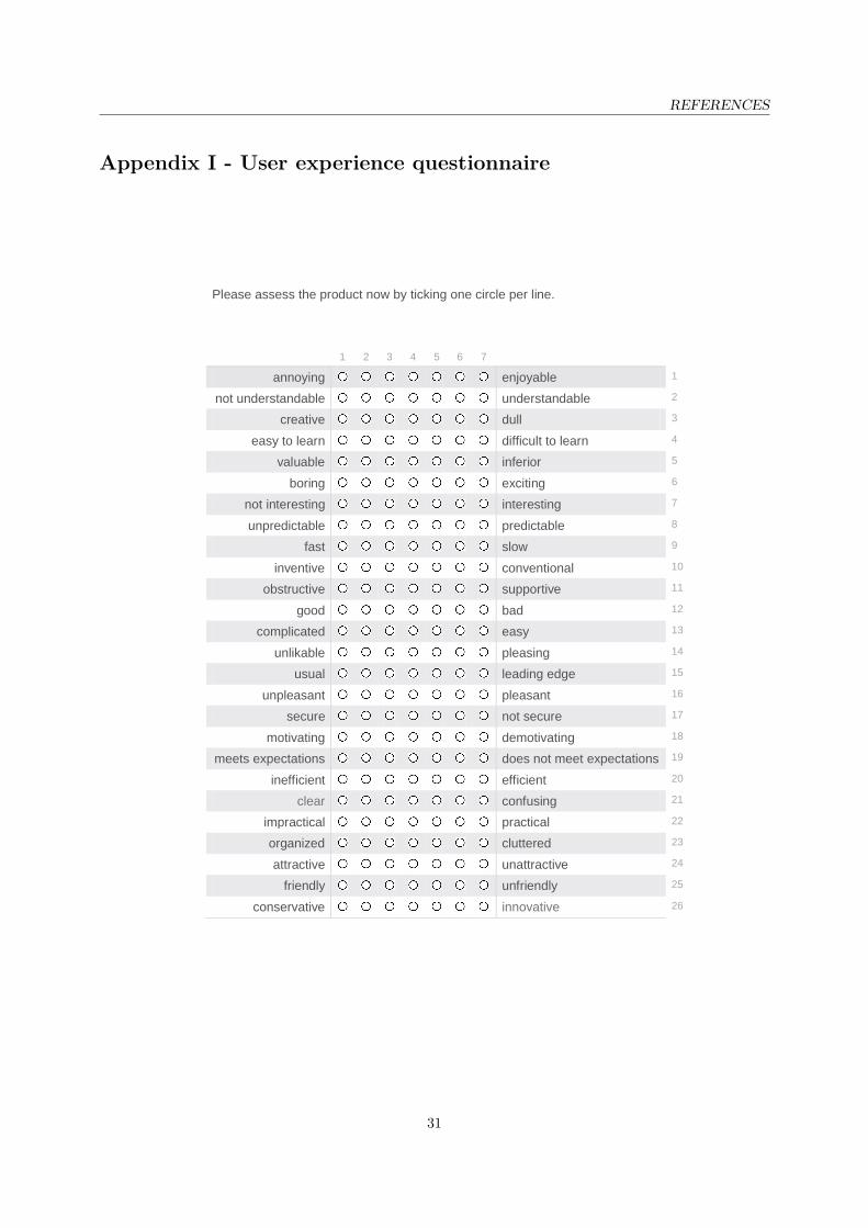
A positive experience with the algorithm and its interface is essential for clinical interpretation. Toevaluate this, the end-user experience questionnaire by Laugwitz et al. (2008)[31] is used. This questionnaire“...should allow the users in a very simple and immediate way to express feelings, impressions, and attitudesthat arise when experiencing the product under investigation [31]”. This is done by a list of 26 items withtwo opposing adjectives with a seven stage scale between them. The English version of this questionnairecan be found in Appendix ii. All these items could be divided in seven domains: attractiveness, perspicuity,efficiency, dependability, stimulation and novelty. Attractiveness represents the overall impression of theproduct and whether it is likeable or not. Perspicuity reflects how easy it is to get familiar with using theproduct. An easy and fast workaround is reflected in efficiency. Dependability is about feeling in controland secure and predictable outcomes. Stimulation is high when it is exciting and motivating to use theproduct and novelty reflects innovation and creativity. Laugwitz et al. also provided a data analysis toolin a Microsoft Excel sheet for correct evaluation of the obtained data. [31]

The questionnaire was filled out by three urologists for version 3 of the gui. Evaluation with thedata analysis tool resulted in a value within a range from -3 to 3 for all seven domains, see Table 4.1.According to Laugwitz et al. a score higher than 0.8 translates to positive evaluation. All scores are muchhigher, resulting in an average overall score of 2.2 reflecting excellent user experience. A contributingfactor could be that two out of three end-users were the urologists involved with improvement of the userinterface. However, for the third urologist this was the first encounter and the predominantly low varianceshows that score was quite like the rest. In Figure 4.5, the mean score for all items of the questionnaire isvisible. This figure explains the higher variance for perspicuity and efficiency. Within efficiency, slow/fasthas a noticeable lower score than other items within that domain. However still positively evaluated, thisreflects room for improvement in performance speed. High variance and the relatively lower score forperspicuity are traced back to the neutral -0.3 score on complicated/easy. The analysis tool recogniseda inconsistency within the domain, indicating that the end-user might misunderstood an item. One userrated complicated/easy with -3. Verbal elucidation on this score pointed out that this user wanted toexpress experiencing the algorithm as sophisticated.

24


Table 4.1: Mean and variance within a range from -3 (horribly bad) to 3 (extremely good) for seven domains ofuser experience.

Domain Mean VarianceAttractiveness 2.4 0.1Perspicuity 1.8 0.8Efficiency 2.2 1.1Dependability 2.1 0.3Stimulation 2.4 0.3Novelty 2.4 0.2

Figure 4.5: Mean score for all adjectives within a range from -3 (horribly bad) to 3 (extremely good) for theseparate adjectives assessing user experience. The seven domains are marked with color, purple for attractiveness,green for perspicuity, dark blue for efficiency, light blue for dependability, red for stimulation and yellow for novelty.

25

CHAPTER 5Outlook and conclusions

5.1 Future recommendationsThe algorithm achieved high approval ratings in this single centre. All of the algorithmic evaluation, itsresulting shape description, the visual substantiation and use of the combining user interface were very wellreceived in umc Utrecht. That is very promising since previously was determined that expert opinion wasnot unambiguous here (Table 2.1). The foundation for the algorithmic evaluations came from consultingarticles and ics standardisation documents. Available information did not cover all aspects or was notunanimous. Choices are made as objectively as possible by basing them on judgements made within theconsensus meetings. This method might have made the algorithm specific for the urology department inUtrecht. Regardless of their different backgrounds the urologists might have different consensus judgementthan elsewhere. This ought to be tested by introducing the algorithmic evaluation in more centres andrepeating evaluation. If it proves to mismatch with urologist interpretation elsewhere, the benefit ofthreshold based evaluation is that these can be easily adapted to match with a wider consensus.

Four descriptors and two additional comments allow for a limited variability. So far it seems sufficientfor specific curve shape description. However, especially since the thresholds are not set in stone, param-eters around threshold value might be of interest. In the current explanatory display is not visible whena parameter approaches threshold value and therefore is for example ‘almost bell shape’. More subtletiesin descriptors might provide extra information for intermittent and fluctuating as well. Currently thesedescriptors apply from one interruption/fluctuation and up and no distinction is made between curveswith 2 or 9 fluctuations. Possible benefit of these nuances should be carefully weighed because it couldmake the algorithmic result more tenuous.

The evaluation excludes inter- and intra observer variability and the generated description has astandardised registration format. This allows reliable comparison of uroflowmetry results and createspossibilities for both comparative research uncovering underlying pathology and clinical follow-up. Inclinical setting, comparison of two or more consecutive uroflowmetry tests can inform about treatmentefficacy or representativeness of voiding. Parameters would easily be reported as e.g. void1 = 17/180/20,void2 = 21/310/0. How important changes in shape descriptions are and whether these are sensitiveto interesting developments are yet unknown. The quantitatively defined descriptors consistently divideuroflowmetry test results into groups, for example fluctuating and not fluctuating. Now diagnoses based onadjunct investigation can be compared for these groups, increasing the diagnostic value of uroflowmetry.

26

CHAPTER 5. OUTLOOK AND CONCLUSIONS

5.2 ConclusionThis study presented an algorithm for automatic uroflowmetry curve shape description. The descriptionis comprised of the descriptors bell shape, fluctuating, intermittent and plateau flow and comments onsymmetry and maximal flow. The corresponding threshold evaluations are as objectively as possibleby combining previously published proposals for shape evaluation. Quantitative definitions for shapecharacteristics that were still missing, are added based on expert consensus. As a result this is the firsturoflowmetry evaluation tool that evaluates all relevant shape characteristics in an entirely reproducibleway, increasing the diagnostic value of uroflowmetry.

A connected user interface makes the algorithmic evaluation insightful for end-users. As a whole it isvery well received in terms of both efficacy and user experience and is ready for clinical implementation.Automatic evaluation makes spreading standardisation easy and the interface invites the user to maintaina conscious look when assessing the uroflowmetry test result.

27

References

[1] W. Schäfer, P. Abrams, L. Liao, A. Mattiasson, F. Pesce, A. Spangberg, A. M. Sterling, N. R.Zinner, and P. v. Kerrebroeck, “Good urodynamic practices: Uroflowmetry, filling cystometry, andpressure-flow studies,” Neurourology and Urodynamics: Official Journal of the International Conti-nence Society, vol. 21, no. 3, pp. 261–274, 2002.

[2] R. Li, Q. Zhu, M. Nibouche, and A. Gammie, “Urine flow rate curve shapes and their descriptors,”Neurourology and urodynamics, vol. 37, no. 8, pp. 2938–2944, 2018.

[3] J. M. Netto, A. Hittelman, S. Lambert, K. Murphy, T. Collette-Gardere, and I. Franco, “Interpretationof uroflow curves: A global survey measuring inter and intra rater reliability,” Neurourology andUrodynamics, 2020.

[4] A. Gammie, P. Rosier, R. Li, and C. Harding, “How can we maximize the diagnostic utility of uroflow?:Ici-rs 2017,” Neurourology and urodynamics, vol. 37, no. S4, pp. S20–S24, 2018.

[5] T. R. Jarvis, L. Chan, and V. Tse, “Practical uroflowmetry.,” BJU international, vol. 110, p. 28, 2012.

[6] A. Wein, L. Kavoussi, A. Novick, A. Partin, and C. Peters, Campbell-Walsh Urology, vol. 3 of Campbell-Walsh Urology. Elsevier Health Sciences, 10 ed., 2011.

[7] W. Boron and E. Boulpaep, Medical Physiology, 2nd Edition. Elsevier Health Sciences, 2012.

[8] Association for Continence Advice, “Understanding continence promotion: Effective management ofbladder and bowel dysfunction in adults.”

[9] M. B. Chancellor, D. A. Rivas, S. G. Mulholland, and W. M. Drake Jr, “The invention of the modernuroflowmeter by willard m. drake, jr at jefferson medical college,” Urology, vol. 51, no. 4, pp. 671–674,1998.

[10] K. Chun, S. J. Kim, and S. T. Cho, “Noninvasive medical tools for evaluating voiding pattern in reallife,” International neurourology journal, vol. 21, no. Suppl 1, p. S10, 2017.

[11] K. Nielsen, R. Bruskewitz, and P. Madsen, “Urodynamics of the lower urinary tract,” Urologicalresearch, vol. 16, no. 4, pp. 271–276, 1988.

[12] M. A. Vijverberg, A. J. Klijn, A. Rabenort, J. Bransen, E. T. Kok, J. P. Wingens, and T. P. de Jong,“A comparative analysis of pediatric uroflowmetry curves,” Neurourology and urodynamics, vol. 30,no. 8, pp. 1576–1579, 2011.

[13] R. Brand, “Uroflowmetry curve analysis of healthy young women,” tech. rep., University of Twente,2014.

[14] J. R. Landis and G. G. Koch, “The measurement of observer agreement for categorical data,” biomet-rics, pp. 159–174, 1977.

[15] M. R. van der Kamp, “Automatic uroflowmetry analysis of women,” tech. rep., University of Twente,2015.

28

REFERENCES

[16] D. C. Boele, “Towards an objective classification algorithm for uroflowmetry curves,” tech. rep.,University of Twente, 2015.

[17] J. S. de Haan, “Clinical validation of algorithmic classification of female uroflowmetry curve patterns,”tech. rep., University of Twente, 2018.

[18] S. P. R. Baas, “A machine learning approach to automatic classification of female uroflowmetrymeasurements,” tech. rep., University of Twente, 2016.

[19] J. van Haaren, “Automatic component based analysis ofuroflowmetry curves in women,” tech. rep.,University of Twente, 2019.

[20] S. D. T. Pham, “Towards more robust detection of relevant voiding time in uroflowmetry curves forimproved automatic analysis,” tech. rep., University of Twente, 2019.

[21] A. Gammie, S. Yoshida, A. Steup, M. Kaper, C. Dorrepaal, T. Kos, and P. Abrams, “Flow timeand voiding time-definitions and use in identifying detrusor underactivity,” in NEUROUROLOGYAND URODYNAMICS, vol. 35, pp. S68–S69, WILEY-BLACKWELL 111 RIVER ST, HOBOKEN07030-5774, NJ USA, 2016.

[22] B. T. Haylen, D. De Ridder, R. M. Freeman, S. E. Swift, B. Berghmans, J. Lee, A. Monga, E. Petri,D. E. Rizk, P. K. Sand, et al., “An international urogynecological association (iuga)/internationalcontinence society (ics) joint report on the terminology for female pelvic floor dysfunction,” Neu-rourology and Urodynamics: Official Journal of the International Continence Society, vol. 29, no. 1,pp. 4–20, 2010.

[23] A. A. Ghobish, “Quantitative and qualitative assessment of flowmetrograms in patients with prosta-todynia,” European urology, vol. 38, no. 5, pp. 576–583, 2000.

[24] K.-E. Jensen, K. Nielsen, H. Jensen, O. Pedersen, and T. Krarup, “Urinary flow studies in normalkindergarten and schoolchildren,” Scandinavian journal of urology and nephrology, vol. 17, no. 1,pp. 11–21, 1983.

[25] R. Babu, S. K. Harrison, and K. A. Hutton, “Ballooning of the foreskin and physiological phimosis: isthere any objective evidence of obstructed voiding?,” BJU international, vol. 94, no. 3, pp. 384–387,2004.

[26] S.-H. Mostafavi, N. Hooman, F. Hallaji, M. Emami, R. Aghelnezhad, M. Moradi-Lakeh, andH. Otukesh, “The correlation between bladder volume wall index and the pattern of uroflowme-try/external sphincter electromyography in children with lower urinary tract malfunction,” Journalof pediatric urology, vol. 8, no. 4, pp. 367–374, 2012.

[27] K. Nishimoto, H. Iimori, S. Ikemoto, and N. Hayahara, “Criteria for differentiation of normal andabnormal uroflowmetrograms in adult men,” British journal of urology, vol. 73, no. 5, pp. 494–497,1994.

[28] P. Abrams, L. Cardozo, M. Fall, D. Griffiths, P. Rosier, U. Ulmsten, P. van Kerrebroeck, A. Victor,and A. Wein, “The standardisation of terminology of lower urinary tract function: report from thestandardisation sub-committee of the international continence society,” Neurourology and Urodynam-ics: Official Journal of the International Continence Society, vol. 21, no. 2, pp. 167–178, 2002.

[29] B. Haylen, D. Ashby, J. R. Sutherst, M. Frazer, and C. West, “Maximum and average urine flow ratesin normal male and female populations—the liverposl nomograms,” British journal of urology, vol. 64,no. 1, pp. 30–38, 1989.

[30] E. M. Biel, “Exploring the diagnostic distinctive possibilities of uroflowmetry,” tech. rep., Universityof Twente, 2019.

29

REFERENCES

[31] B. Laugwitz, T. Held, and M. Schrepp, “Construction and evaluation of a user experience question-naire,” in Symposium of the Austrian HCI and Usability Engineering Group, pp. 63–76, Springer,2008.

30

REFERENCES

Appendix I - User experience questionnaire

Please assess the product now by ticking one circle per line.

1 2 3 4 5 6 7

annoying enjoyable 1

not understandable understandable 2

creative dull 3

easy to learn difficult to learn 4

valuable inferior 5

boring exciting 6

not interesting interesting 7

unpredictable predictable 8

fast slow 9

inventive conventional 10

obstructive supportive 11

good bad 12

complicated easy 13

unlikable pleasing 14

usual leading edge 15

unpleasant pleasant 16

secure not secure 17

motivating demotivating 18

meets expectations does not meet expectations 19

inefficient efficient 20

clear confusing 21

impractical practical 22

organized cluttered 23

attractive unattractive 24

friendly unfriendly 25

conservative innovative 26

31

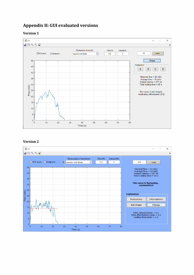
Appendix II: GUI evaluated versions

Version 1

Version 2

REFERENCES

Appendix III - Generation of reference flow curve

Formula for Qmax according to Liverpool nomograms. Value 6 is added to adjust for translation later on.Women: Qmax, ref = 6 + exp(0.511 + 0.505· log(volume))Men: Qmax, ref = 6 + (2.37 + 0.18 ∗

√volume− 0.014· age)2

Formula for normal distribution (bell shape):Qref = Qmax, ref · exp((−(t−µ)2)/(2∗sd2)); with µ = 0.5· voiding time and sd empirically determinedto make volume of reference curve agree with true voided volumes:

Women: sd = 0.01· volume+ 4Men: sd = 0.008· volume+ 6

To represent uroflowmetry, the graph represented as Qref = f(t) is translated: Qref + 6 = f(t-µ)

The accepted deviaton from Qref, according to the quarter percentiles in the nomogram for volumes100-600 ml:

Women: deviation(volume) = 4 + (6/500· (volume− 100))Men: deviation(volume) = 4 + (2/500· (volume− 100))

33

Appendix IV – Manuscript sub study fluctuation thresholds

Evaluation of quantitative thresholds for defining fluctuations in

uroflowmetry curves

J.S. de Haan1,2, P.F.W.M. Rosier1, B.J. Geurts3, L.M.O. de Kort1

1. Department of Urology, C04.236, University Medical Centre Utrecht, P.O. Box 85500, 3508GA, the

Netherlands

2. Technical Medicine, University of Twente, Enschede, The Netherlands. Mail:

[email protected]

3. Multiscale Modeling and Simulation, Faculty EEMCS, University of Twente, P.O. Box 217, 7500 AE

Enschede, The Netherlands

Abstract

Objectives: A variety of shape descriptors apply to fluctuations in urine flow rate. There is no

unanimity for a cut-off that quantitatively defines this flow shape. This study aims at evaluating the

current thresholds and proposing a universal quantitative threshold for fluctuations in uroflowmetry

curves to increase objectivity of uroflowmetry interpretation and open up possibilities in

comparative research.

Methods: In a single centre study, 219 uroflowmetry measurements of patients in the outpatient

clinic with lower urinary tract symptoms were evaluated. Fluctuation detection was applied using

three thresholds for the change in flow rate: the square root of maximum flow, 20% of maximum

flow and 5 ml/s. The number of fluctuations as well as descriptive outcome are compared between

the thresholds and with expert consensus.

Results: Classification of the curve shape as fluctuating or not resulted in agreement between

outcomes of the three thresholds for 82% of all included flow curve. Comparison of the remaining

cases against consensus classification resulted in agreement between 32% and 63% with the

threshold outcomes.

Conclusion: The three quantitative threshold options are not interchangeable. Due to threshold

dependency on maximal flowrate, sensitivity varies. Based on expert opinion and sensitivity for the

most common range maximal flowrate range of curves it is proposed to consider a fluctuation larger

than 20% of the maximal flow rate as the shape defining characteristic of choice.

Introduction

Uroflowmetry is a test to provide quantitative information about voiding function in patients with

lower urinary tract symptoms. Apart from parameters as maximum flow rate, voided volume and

voiding time to separate normal from abnormal, the shape of the uroflowmetry flow rate curves can

also indicate voiding abnormalities [1]. However, currently there is no standard for describing

abnormal flow shapes. Diagnosis of flow shape abnormalities is therefore operator dependent.

Consequently, flow shapes are described inconsistently in literature. Li et al. (2018)[2] researched

articles and International Continence Society (ICS) standardisation documents for observed flow

shapes and the corresponding descriptors used. There is likewise considerable variability in

quantitative definitions for the shapes, when presented, as in descriptors used for comparable flow

shapes. This is troubling comparative research, for example aimed at discovering pathophysiology

associated with the curve patterns. When application of descriptors is clearly defined it becomes

valuable to associate them with diagnoses nowadays made based on more invasive investigations.

[2]

The shape descriptor that is subject of this article is ‘fluctuating’. According to the ICS it applies to a

continuous urine flow having multiple peaks [1]. When flow rate decreases and increases rapidly this

causes a local peak in the time flow rate graph. Other terminology describing similar shape

characteristics is: ‘staccato’, ‘multiple peak’, ‘intermittent’, ‘sawtooth’, ‘undulating’ and multiphasic

[2,3]. Four articles discussed in the review by Li et al. provided quantitative thresholds. These

thresholds are the square root of maximum flow, 20% of maximum flow and 5 ml/s [4-7]. When a

variation in flow rate exceeds the threshold, it is considered a fluctuation.

These differences in thresholds may result in differences in recognising patterns of fluctuations and

therefore in a different shape description for the uroflowmetry curve. The present study investigates

the differences that are consequent to the three described thresholds and proposes a substantiated

choice for a universally applicable threshold.

Methods

Uroflowmetry data used in this study are recent measurements of patients with lower urinary tract symptoms visiting the urology outpatient clinic of the University Medical Centre Utrecht. All uroflowmetry measurements in the period from begin July to mid-September 2019 with a voided volume above 100 ml are included, there is no selection on symptoms or diagnosis. Data is fully anonymous except for gender. All patients are over 18 years old. Uroflowmetry was done when patients felt normal desire to void. They were instructed to void like they normally would on a regular toilet, in a position of their preference. Measurements are performed on the FlowClean uroflowtoilet (Urotex, The Netherlands). This weight sensor device has a sample rate of 10 Hz, embedded software applies a moving average filter with one second window length. All three quantitative thresholds used to define fluctuations reported in the review by Li et al. are used for comparison. Two evaluated thresholds are in terms of the maximal flow rate (Qmax), found as the highest value in the measurements flow vector. The first threshold (ThSq) is equal to the square root of Qmax in ml/s [4,5]. The second threshold (Th20p) is equal to 20% of Qmax in ml/s [6] and the third (Th5) is equal to 5 ml/s [7].

Fluctuations were identified by detection of their peaks. Peak detection was executed with the MATLAB (version 2018b, Mathworks, USA) built in function findpeaks. This function finds local maxima by comparing sample values with adjacent values. To limit detected fluctuations to only the ones exceeding the researched thresholds, the setting MinPeakProminence was used. The decrease in flow rate is calculated. On either side, within the time segment from the potential peak to the point where the signal attains a higher value or the end of the signal the lowest value is found. The difference between the highest of the two and peak value is the prominence of that peak. Peak detection is limited to peaks where the prominence is at least as large as the threshold value. The function has two output arguments: peak values and their corresponding timestamps. [8] Based on the previously mentioned ICS definition, peak detection is applied only to periods of continuous urine flow. This means that in case of interrupted flow measurements, just the uninterrupted flow part with the largest volume was evaluated. The number of fluctuations equals the number of detected peaks minus the peak corresponding with the maximal flow. Therefore the term additional peaks is used for all detected peaks exceeding the threshold value next to the peak corresponding to Qmax. According to definition, presence of one additional peak is enough to classify as fluctuating. This causes a dichotomous distinction of curves between one or more additional peaks and no additional peaks. To further research threshold differences, the number of additional peaks detected per threshold is determined and compared. Consensus meeting Since there is no unique, generally agreed, recommendation for the threshold value to be used, no standard method in clinical application can be assumed. Therefore, classifications of uroflowmetry curves as fluctuating or not that are conflicting between the thresholds is compared to clinical team judgement. These reference judgements followed from a consensus meeting with four medical doctors of the urology department of University Medical Centre Utrecht under supervision of the first author, referred to as ‘researcher’. These doctors are tasked with interpretation of uroflowmetry measurements in their day-to-day work. Subject for the meeting are curves where the three thresholds did not agree about the presence of additional peaks (zero versus one or more). The uroflowmetry measurement curve was shown on a large screen. Question for each curve was whether the team would classify that curve as fluctuating, given the explanation that this means the curve has one or more relevant fluctuations. This applies to fluctuations that might be clinically relevant so the urologist would not want to miss it in analysis. The attendants discussed about the pattern of fluctuations in the curve. When the discussion tended to either a yes or no answer, this was proposed by the researcher as final answer. When none of the attendants objected this was noted as an unambiguous yes or no. When one or more team members did object, discussion continued and this step was repeated once more. When there was no consensus by then was concluded that consensus could not be reached and the curve was excluded from analysis. Statistics Statistical analysis of the peak detection outcomes was performed with SPSS Statistics (version 25, IBM, USA). To test whether the differences in the number of additional peaks detected for each of the three thresholds is significant, the distributions are compared between themselves. Each distribution is the collection of the number of additional peaks for all the curves per threshold. Each value per threshold is related to a value in the two other distributions, the values representing the number of additional peaks according to the other thresholds. Additionally, the distributions contain nominal data and are not normally distributed. Therefore was chosen to adopt Friedman's two-way non-parametric ANOVA. Post hoc analysis for when this test showed a significant difference was done with the Bonferroni-corrected Dunn's test.

The three distributions reflecting the presence or absence of additional peaks according to the three thresholds are as well related and not normally distributed. Unlike the previous comparison these distributions are binominal instead of nominal. Differences in these distributions are therefore analysed by means of Cochran’s Q test. In case of a significant difference, post hoc pairwise comparison was performed with McNemar’s test for related samples. For all statistical analyses a significance level of p < 0.05 will be regarded.

Results

Descriptive Inclusion criteria were met by 222 curves. Three curves had to be excluded due to measurement errors. These were recognised as such because the flow measurements reflected physically impossible voiding. As a result, 219 uroflowmetry measurements were available for analysis. Of these measurements 145 (66%) were of male patients. Maximal flow rate for the total group of measurements was 19.3 ± 10.9 ml/s (mean ± s. d.). The maximal flow rate determines the value of two of the three thresholds. The graph in Figure 1 visualizes the dependency of the threshold value on the maximal flow. Fluctuations above the lines are detected. The histogram below shows the number of curves with Qmax in a certain range.

Figure 1: Top: All three threshold values in ml/s as function of maximum flow. The threshold is the lowest value that is considered a fluctuation. Bottom: Histogram representing the number of curves with maximal flow in a certain range.

Number of peaks In 120 cases (55%) all three threshold definitions resulted in the same number of additional peaks per curve. Of these cases, for 73 curves this number is zero. For all 219 curves the frequencies of curves per number of detected fluctuations can be seen in Figure 2. Friedman’s repeated measures ANOVA was used to compare these outcomes between the thresholds. Bonferroni corrected significance values are presented in Table 1. It shows that the number of detected additional peaks differed significantly for the three different thresholds (p < 0.001). Dunn-Bonferroni post hoc tests were carried out and there were significant differences between Th20p and the other two thresholds. The difference between ThSq and Th5 is not significant with Bonferroni corrected p-value 0.23. This means that the threshold equal to 20% of Qmax is most distinct compared to the other two.

Figure 2: Histogram for the frequencies of curves per number of detected fluctuations resulting from the three thresholds.

Table 1: Dunn's test pairwise comparison of detected peaks per threshold. Displayed is Bonferroni corrected significance. This underpins that ThSq and Th5 are comparable with each other and Th20p is distinguishably different.

Significance

ThSq – Th20p 0.001

ThSq – Th5 0.231

Th20p – Th5 0.000

Presence of peaks In 146 of the curves at least one of the three threshold definitions resulted in detection of peaks next to the maximal flow peak. Comparison of the dichotomous notation for the three thresholds for the presence of additional peaks resulted in agreement in 179 curves (82%). In Table 2 the frequencies of flow rate curves with and without additional peaks are shown for all three thresholds.

0

20

40

60

80

100

120

0 1 2 3 4 5 6 7 8 9 >9

Nu

mb

er o

f cu

rves

Number of detected fluctuations

ThSq

Th20p

Th5

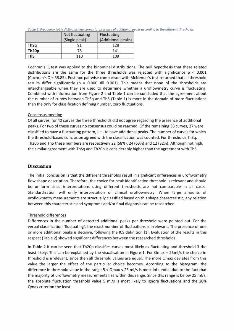
Table 2: Frequency table distinguishing curves for presence of additional peaks according to the different thresholds.

Not fluctuating (Single peak)

Fluctuating (Additional peaks)

ThSq 91 128

Th20p 78 141

Th5 110 109

Cochran’s Q test was applied to the binominal distributions. The null hypothesis that these related distributions are the same for the three thresholds was rejected with significance p < 0.001 (Cochran’s Q = 38.85). Post hoc pairwise comparison with McNemar’s test returned that all threshold results differ significantly (p = 0.000 till 0.001). This means that none of the thresholds are interchangeable when they are used to determine whether a uroflowmetry curve is fluctuating. Combined with information from Figure 2 and Table 1 can be concluded that the agreement about the number of curves between ThSq and Th5 (Table 1) is more in the domain of more fluctuations than the only for classification defining number, zero fluctuations. Consensus meeting Of all curves, for 40 curves the three thresholds did not agree regarding the presence of additional

peaks. For two of these curves no consensus could be reached. Of the remaining 38 curves, 27 were

classified to have a fluctuating pattern, i.e., to have additional peaks. The number of curves for which

the threshold-based conclusion agreed with the classification was counted. For thresholds ThSq,

Th20p and Th5 these numbers are respectively 22 (58%), 24 (63%) and 12 (32%). Although not high,

the similar agreement with ThSq and Th20p is considerably higher than the agreement with Th5.

Discussion

The initial conclusion is that the different thresholds result in significant differences in uroflwometry

flow shape description. Therefore, the choice for peak identification threshold is relevant and should

be uniform since interpretations using different thresholds are not comparable in all cases.

Standardisation will unify interpretation of clinical uroflowmetry. When large amounts of

uroflowmetry measurements are structually classified based on this shape characteristic, any relation

between this characteristic and symptoms and/or final diagnosis can be researched.

Threshold differences

Differences in the number of detected additional peaks per threshold were pointed out. For the

verbal classification ‘fluctuating’, the exact number of fluctuations is irrelevant. The presence of one

or more additional peaks is decisive, following the ICS definition [1]. Evaluation of the results in this

respect (Table 2) showed significant differences between the researched thresholds.

In Table 2 it can be seen that Th20p classifies curves most likely as fluctuating and threshold 3 the

least likely. This can be explained by the visualisation in Figure 1. For Qmax = 25ml/s the choice in

threshold is irrelevant, since then all threshold values are equal. The more Qmax deviates from this

value the larger the effect of the particular choice becomes. According to the histogram, the

difference in threshold value in the range 5 < Qmax < 25 ml/s is most influential due to the fact that

the majority of uroflowmetry measurements lies within this range. Since this range is below 25 ml/s,

the absolute fluctuation threshold value 5 ml/s is most likely to ignore fluctuations and the 20%

Qmax criterion the least.

It is beneficial to incorporate the dominant range of Qmax in the choice between threshold options

since Qmax does not vary over a very wide range. For the total group of measurements we observed

Qmax = 19.3 ± 10.9 ml/s. In a study of Kumar et al. who reported peak urinary flow rate for a larger

male and female group, Qmax values were 22.8 ± 9.33 ml/sec and 20.53 ± 7.75 ml/sec, respectively

[9]. These values might be somewhat higher since symptom free participants were included.

Expert interpretation

All of the quoted articles fail to provide physiolocial substantiation for the chosen thresholds [4-7].

Therefore, it makes sense to consult physicians with yearlong experience of interperting

uroflowmetry measurements. Furthermore, implementation of scientific results in patient

diagnostics benefits from involvement of physicians in the research [10]. Limitation of this approach

is that the reference rating could be subjective for this small group that works in the same hospital.

Future work, including more experts from a wider range of teams will substantiate the reference

interpertation.

Th5 was evidently less supported by the clinicians than the other two. The level of agreement was

only 32% compared to 58% and 63% for ThSq and Th20p respectively. The absolute threshold 5 ml/s

is not sensitive enough to detect fluctuations in low-flow voiding patterns.

Clinical relevance The choice between ThSq and Th20p is less obvious. However since the assessments baed on these

thresholds resemble eachother quite closely (see Table 2) the distinction is also less critical.

Comparison with the concensus reference showed a small preference for threshold 2. Most

important is that a choice is made and that the use of this threshold is standardised.

An argument in favor of Th20p is that it is more sensitive to fluctuations in the primary range of

maximal flowrate values. When automatic detection of peaks results in labelling the curve as

fluctuating, this indicates a possible pathological situation. The findings can be placed into clinical

context to interpretet the shape characteristic. Anyway, detection prompts the urologist to look

more closely at the uroflowmetry and therefore false positives are better than false negatives.

For optimal implementation, automatic comparison of fluctuations prominence with the threshold

like in this research is essential. Uroflowmetry devices do report Qmax and 20% is easily calculated.

However, the precise size of a fluctuation is not easily determined from a time flow rate graph.

Additionally, automatic evaluation is faster and makes less errors.

Conclusion

Whether or not a uroflowmetry curve is interpreted as fluctuating is dependent on the quantitative threshold definition used. Both clinical diagnosis and associative research would therfore benefit from a standardised threshold. Based on expert opinion and sensitivity for the most prevalent curves it is proposed to consider a fluctuation larger than 20% of the maximal flow rate as the most appropriate shape defining characteristic. This value is now dictated by choice. Future knowledge of underlying physiology or experiences while using this threshold type could serve in optimisation of this value.

References

1) Abrams P, Cardozo L, Fall M, et al. The standardisation of terminology of lower urinary tract function. Neurourol Urodyn.2002;21:167–178.

2) Li, R., Zhu, Q., Nibouche, M. and A. Gammie, “Urine flow rate curve shapes and their descriptors," Neurourology and Urodynamics, 2018.

3) Rollema HJ. Uroflowmetry in males: Reference values and clinical application in benign prostatic hypertrophy. [S.n.], 1981. 287 p.

4) Austin PF, Bauer SB, Bower W, et al. The standardization of terminology of lower urinary tract function in children and adolescents: update report from the Standardization Committee of the International Children's Continence Society. J Urol. 2014;191:1863–1865.

5) Mostafavi SH, Hooman N, Hallaji F, et al. The correlation between bladder volume wall index and the pattern of uroflowmetry/external sphincter electromyography in children with lower urinary tract malfunction. J Pediatr Urol. 2012;8:367–374.

6) Fantl JA, Smith PJ, Schneider V, Hurt WG, Dunn LJ. Fluid weight uroflowmetry in women. Am J Obstet Gynecol. 1983;145: 1017–1024.

7) Mattsson S, Spångberg A. Urinary flow in healthy schoolchildren. Neurourol Urodyn. 1994;13:281–296.

8) Mathworks, MATLAB documentation: Findpeaks, https://nl.mathworks.com/help/signal/ref/findpeaks.html#d117e66057, cited 3-12-2019

9) Kumar V, Dhabalia JV, Nelivigi GG, Punia MS, Suryavanshi M. Age, gender, and voided volume dependency of peak urinary flow rate and uroflowmetry nomogram in the Indian population. Indian J Urol. 2009;25(4):461–466. doi:10.4103/0970-1591.57912

10) Dinant, GJ., Hopstaken, R. & van Bokhoven, L. HUWE (2004) 47: 918. https://doi.org/10.1007/BF03084045

Documents

OF UROFLOWMETRY CURVE SHAPES