Embed Size (px)
Citation preview
A POSTERIORI ERROR ESTIMATIONS FOR FINITE ELEMENT
APPROXIMATIONS ON QUADRILATERAL MESHES
UDC 519.624.2
H.A. SHYNKARENKO AND O.V.VOVK
Abstract. The main goal of this paper is to construct the simple a posteriori errorestimators for piecewise bilinear approximations of nite element method whichare able to reliably and eciently calculate the two-sided condence interval forthe approximation error of the elliptic boundary value problems. Under assumptionthat nite element method scheme can calculate the exact values of a solution atmesh nodes, we propose the element-wise error estimators of Dirihlet and Neuman,which are calculated in succession as the approximated solutions of the residualproblem of nite element method approximations. The rst of them evaluate thelower bound of the nite element approximation error and second evaluate the upperbound. We supplement the characteristics of this estimators by the detailed resultsof the numerical experiments with semi-linear and singularly perturbed problemswith boundary and internal layers.
Àíîòàöiÿ. Îñíîâíîþ ìåòîþ öi¹¨ ïðàöi ¹ ïîáóäîâà ïðîñòèõ àïîñòåðiîðíèõ îöiíþ-âà÷iâ ïîõèáîê ÷àñòèíàìè áiëiíiéíèõ àïðîêñèìàöié ìåòîäó ñêií÷åííèõ åëåìåíòiâ,çäàòíèõ íàäiéíî òà åôåêòèâíî îá÷èñëþâàòè äâîñòîðîííi ãðàíèöi ïîõèáîê íàáëè-æåííÿ ðîçâ'ÿçêiâ åëiïòè÷íèõ êðàéîâèõ çàäà÷. Çà äîïóùåííÿ, ùî ñõåìà ìåòîäóñêií÷åííèõ åëåìåíòiâ ñïðîìîæíà îá÷èñëèòè òî÷íi çíà÷åííÿ ðîçâ'ÿçêó ó âóçëàõñiòêè, çàïðîïîíîâàíî ïîåëåìåíòíî âèçíà÷åíi îöiíþâà÷i ïîõèáîê Äiðiõëå òà Íå-éìàíà, ÿêi ïîñëiäîâíî îá÷èñëþþòüñÿ ÿê íàáëèæåíi ðîçâ'ÿçêè çàäà÷i ïðî ëèøîêàïðîêñèìàöi¨ ìåòîäó ñêií÷åííèõ åëåìåíòiâ. Ïåðøèé ç íèõ çíàõîäèòü íèæíþ ãðà-íèöþ ïîõèáêè àïðîêñèìàöi¨ ìåòîäó ñêií÷åííèõ åëåìåíòiâ, à äðóãèé - âåðõíþãðàíèöþ. Ìè äîïîâíþ¹ìî õàðàêòåðèçàöiþ öèõ îöiíþâà÷iâ äåòàëüíèìè ðåçóëü-òàòàìè ÷èñëîâèõ åêñïåðèìåíòiâ ç ñëàáêî íåëiíiéíîþ òà ñèíãóëÿðíî çáóðåíèìèçàäà÷àìè ç ïðèìåæåâèìè i âíóòðiøíiìè øàðàìè.
This work is dedicated to R. S. Chapko on the occasion of his ftieth birthday.
1. Introduction
A posteriori error estimations of nite element method (FEM) approximations is theimportant component of a modern science calculations. The Babuska's and Rheinboldt's ori-ginal conception of a posteriori error estimation (1978) in the last decades generates a largefamily of various a posteriori error estimators (AEEs), which are able to qualitatively describethe errors of obtained approximations by FEM and create the foundation for local triangulati-on renement and\or local renement of approximations rates such that to nd approximativesolutions with guaranteed accuracy and minimal computational cost, see [2], [3], and also [4].
Following the previous work [8] we build element-wise Dirihlet εDirh and Neuman εNeu
h aposteriori error estimators for piece-wise bilinear nite element approximations on quadrilateralmeshes. These estimators are able to qualitatively calculate the lower and upper bounds of exacterror in terms of the following inequality
εDirh ≤∥ u− uh ∥≤ εNeu
h . (1.1)
†Key words. semi-linear diusion-advection-reaction equation, variational problem, nite elementmethod, Newton's method, generalized minimum residual method, element-wise a posteriori error esti-mator, eciency index, convergence rate.
1
This paper is structured in the following manner. In Section 2 we formulate the variationalproblem for elliptic diusion-advection-reaction equation with semi-linearity and describe itsfeatures. The numerical scheme with quadrilateral nite elements is presented in Section 3. Thenext (Section 4) is devoted to the problem of the error estimation of FEM approximations. InSections 5 and 6 we present element-wise solutions of this problem as the polynomial Dirihletand Neuman indicator functions. The rest of the paper is devoted to the analysis of numericalexperiments with the boundary value problems which require some eorts for solving because theyare semi-linear or singularly perturbed. A comparison of characteristics of the estimators and theyanalogues, which are calculated for exact values of errors conrms the possibility of the calculationof two-sided error estimates (1.1) and expected convergence rates of FEM approximations.
2. Problem statement
To construct the cheap a posteriori error estimators for two-sided error estimates of niteelement approximations we consider a singular perturbed and\or semi-linear boundary valueproblems with second order elliptic equation
−∇.(µ∇u) + β.∇u+ σu = f [u] in Ω
u = 0 on ΓD,
−(µ∇u).ν = q on ΓN = ∂Ω\ΓD.
(2.1)
This semi-linear boundary value problem has the following variational formulationnd u ∈ V = v ∈ H1(Ω) : v = 0 on ΓD such that
a(u, v) = ⟨N [u], v⟩ ∀v ∈ V,(2.2)
where a(u, v) : =
∫Ω
[(µ∇u).∇v + v(β.∇u+ σu)]dx,
⟨N [w], v⟩ : =∫Ω
f [w]vdx−∫ΓN
qvdγ.
Below we assume that the domain Ω ⊂ R2 is a bounded polygon and other problem data aresuciently regular functions to guarantee existence and uniqueness of the solution u = u(x, y)that satises (2.2). We note here that the problem (2.2) becomes singularly perturbed in the case∥β∥L∞(Ω) → +∞ or/and ∥σ∥L∞(Ω) → +∞, for the details we refer to [7].
3. Finite element approximations
In order to obtain approximations of the solution u of the variational problem (2.2) we use thefamily of quasiuniform meshes Th, which are composed of quadrilateral elements Q, Th = Q,hQ = diam Q, h = maxhQ. Now for each m ∈ N we can construct the nite element space
V 1h :=
v ∈ V ∩ C(Ω) : v =
∑i,j=0,1
aijxiyj ∀aij ∈ R, ∀(x, y) ∈ Q, ∀Q ∈ Th
with usual basis functions
φ1, ..., φM ∈ V 1h , supp φi := Ωi = ∪Q : Ai ∈ Q, φj(Ai) = δij , (3.1)
where M is a number of nodes Ai = (xi, yi) of the mesh Th, which does not lie on a boundarypatch ΓD.
Then, using Galerkin discretization procedure, we reduce (2.2) to the following problemnd uh ∈ V 1
h such that
a(uh, v) = ⟨N [uh], v⟩ ∀v ∈ V 1h
(3.2)
2
or in the algebraic form:nd uh =
M∑i=1
qiφi such that
the coecients qiMi=1 ∈ RMsatisfy∑M
j=1a(φj , φi)qj = ⟨N [uh], φi⟩, i = 1, ...,M.
(3.3)
In order to unify computing process of the coecients qi ∈ R, i = 1, ...,M , we use the so called'master element' Q0 = (α, β) ∈ R2 : |α|, |β| ≤ 1 with the mapping Φ : Q0 → Q as follows
x(α, β) =∑
i,j=±1
x 12(5+2j−ij)(1 + iα)(1 + jβ),
y(α, β) =∑
i,j=±1
y 12(5+2j−ij)(1 + iα)(1 + jβ),
where Am = (xm, ym), m = 1, ..., 4 are the vertices of the quadrilateral Q. The integrals from(3.3) that dened in the variational problem (2.2) are calculated numerically by using Gaussquadratures on master element Q0.
To solve the problem (3.3) we rewrite it in the following matrix form:
nd vector q ∈ RMsuch that Sq = F [q], (3.4)
where the matrix S = SkmMk,m=1 and the vector F [q] = Fk[q]Mk=1 are obtained in the followingrules
Skm :=
∫Ωmk
[(µ∇ϕm).∇ϕk + (β.∇ϕm + σϕm)ϕk]dx, Ωmk := Ωm ∩ Ωk,
Fk[w] :=
∫Ωk
f
[N∑i=1
wiϕi
]ϕkdx+
∫Γq∩∂Ωk
gϕkdγ, k,m = 1, ...,M.
The last one can be solved by Newton's method which is written as the following iterative processwith the initial guess q0 ∈ RM and the relaxation parameter τ
given vector qn ∈ RM , τ = const > 0;
nd vector r ∈ RMsuch that
S − τFq[qn]r = F [qn]− Sqn,
qn+1 = qn + τr, n = 0, 1, ...,
(3.5)
where Fq[q] :=
∂Fk[q]∂qm
M
k,m=1is the Jacobi matrix with components
∂Fk[q]
∂qm=
∫Ωmk
∂f
∂u
[M∑i=1
qiϕi
]ϕmϕkdx, k,m = 1, ...,M, q ∈ RM .
At each iteration of the Newton's method we solve the system of linearized equations (3.5) by theiterative solver, namely the generalized minimal residual method (GMRES) [14]. A preconditionerfor this linear system is constructed using incomplete LU factorization.
4. Residual element-based estimator
We dene the error eh = u − uh, which is the solution of the following nonlinear errorproblem [1,4, 5]:
nd eh ∈ Eh ⊂ E, V = E ⊕ Vh such that
a(eh, v) = ⟨N [uh + eh], v⟩ − a(uh, v) ∀v ∈ Eh.
3
Applying Taylor's formula f [eh+uh] = f [uh]+fu[uh]eh+O(e2h), we obtain the linear problemnd error estimator eh ∈ Eh such that
b(uh; eh, v) = ⟨ρ[uh], v⟩ ∀v ∈ Eh,(4.1)
where b(w; z, v) : = a(z, v)−∫Ω
fu[w]zvdx,
⟨ρ[w], v⟩ : = ⟨N [w], v⟩ − a(w, v) ∀w, z, v ∈ V.
In order to obtain the two-sided condence interval for the approximation error we introduceboth Dirihlet ϵDir
h and Neuman ϵNeuh element-based residual error indicator functions that get
lower and upper error bounds correspondingly. They are the approximate solutions of the problem(4.1) for two dierent nite dimensional subspaces EDir
h ⊆ Eh and EDirh ⊆ Eh and are obtained
as the solutions of the following local problems:nd ϵDir
Q ∈ EDirh (Q) := v ∈ H1(Q) : v = 0 on ∂Q such that
b(uh; ϵDirQ , v) = ⟨ρ[uh], v⟩ ∀v ∈ EDir
h (Q), ∀Q ∈ Th,(4.2)
and nd ϵNeu
Q ∈ ENeuh (Q) := v ∈ H1(Q) : v(Ai) = 0 ∀Ai ∈ Q such that
b(uh; ϵNeuQ , v) = ⟨ρ[uh], v⟩ ∀v ∈ ENeu
h (Q), ∀Q ∈ Th,(4.3)
corispondingly. The solutions of the problems (4.2) and (4.3) are unique and exist on each niteelement Q ∈ Th . Also, we can dene the single element indicator ηQ := ∥ϵQ∥1,Q ∀Q ∈ Th
and the global estimator ∥ϵh∥21,Ω :=∑
Q∈Thη2Q ∀Th for both of them. This a posteriori error
estimators come from the original concept of a posteriori error estimation, which was proposedin [2, 3], and is similar to the residual estimators based on a local Dirichlet boundary valueproblem, see [4]. The novelty is in the behaviour of interpolation on the edges of elements: theconstructed Dirihlet error estimator ϵDir
Q (4.2) vanishes at all boundary of nite element Q andNeuman estimator ϵNeu
Q (4.3) vanishes only at the nodes of Q ∈ Th. The similar idea was proposedin [8, 9] for triangular meshes.
5. Computable estimator for piecewise bilinear approxi-
mations
Now we consider the nite element approximation uh ∈ V 1h , which is written in local coordi-
nates (α, β) of the quadrilateral Q ∈ Th as follows
uh|Q = uQ(α, β) =∑
i,j=±1uh(A 1
2(5+2j−ij))(1 + iα)(1 + jβ).
To compute the solutions of of the problems (4.2) and (4.3), in a general case we dene theindicator function ϵh on each nite element Q in the local manner
ϵh|Q = ϵQ(α, β) := λQϕQ(α, β) ∈ Eh(Q) ∀(α, β) ∈ Q0, λQ ∈ R, (5.1)
where ϕQ(α, β) is the quadratic function on master element Q0. Then, from local problem (4.2)or (4.3) we can obtain the coecients λQ on each nite element of the following general kind
λQ =⟨ρ[uh], ϕQ⟩
b(uh;ϕQ, ϕQ)∀Q ∈ Th,
and dene the element error indicator ηQ and the global error estimation ∥ϵh∥1,Ω
ηQ = ∥ϵQ∥1,Q = |λQ| ∥ϕQ∥1,Q ∀Q ∈ Th, ∥ϵh∥21,Ω =∑
Q∈Th
η2Q ∀Th.
4
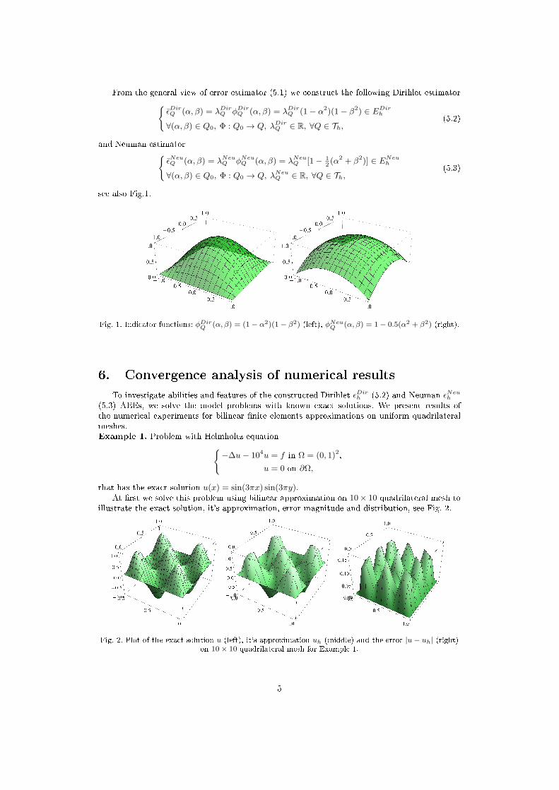
From the general view of error estimator (5.1) we construct the following Dirihlet estimatorϵDirQ (α, β) = λDir
Q ϕDirQ (α, β) = λDir
Q (1− α2)(1− β2) ∈ EDirh
∀(α, β) ∈ Q0, Φ : Q0 → Q, λDirQ ∈ R, ∀Q ∈ Th,
(5.2)
and Neuman estimatorϵNeuQ (α, β) = λNeu
Q ϕNeuQ (α, β) = λNeu
Q [1− 12(α2 + β2)] ∈ ENeu
h
∀(α, β) ∈ Q0, Φ : Q0 → Q, λNeuQ ∈ R, ∀Q ∈ Th,
(5.3)
see also Fig.1.
Fig. 1. Indicator functions: ϕDirQ (α, β) = (1− α2)(1− β2) (left), ϕNeu
Q (α, β) = 1− 0.5(α2 + β2) (right).
6. Convergence analysis of numerical results
To investigate abilities and features of the constructed Dirihlet ϵDirh (5.2) and Neuman ϵNeu
h
(5.3) AEEs, we solve the model problems with known exact solutions. We present results ofthe numerical experiments for bilinear nite elements approximations on uniform quadrilateralmeshes.Example 1. Problem with Helmholtz equation
−∆u− 104u = f in Ω = (0, 1)2,
u = 0 on ∂Ω,
that has the exact solution u(x) = sin(3πx) sin(3πy).At rst we solve this problem using bilinear approximation on 10× 10 quadrilateral mesh to
illustrate the exact solution, it's approximation, error magnitude and distribution, see Fig. 2.
Fig. 2. Plot of the exact solution u (left), it's approximation uh (middle) and the error |u− uh| (right)on 10× 10 quadrilateral mesh for Example 1.
5
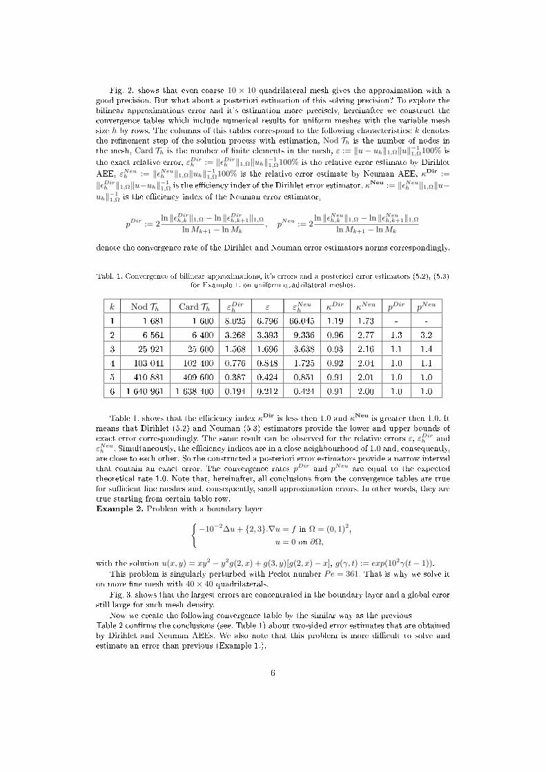
Fig. 2. shows that even coarse 10 × 10 quadrilateral mesh gives the approximation with agood precision. But what about a posteriori estimation of this solving precision? To explore thebilinear approximations error and it's estimation more precisely, hereinafter we construct theconvergence tables which include numerical results for uniform meshes with the variable meshsize h by rows. The columns of this tables correspond to the following characteristics: k denotesthe renement step of the solution process with estimation, Nod Th is the number of nodes inthe mesh, Card Th is the number of nite elements in the mesh, ε := ∥u− uh∥1,Ω∥u∥−1
1,Ω100% is
the exact relative error, εDirh := ∥ϵDir
h ∥1,Ω∥uh∥−11,Ω100% is the relative error estimate by Dirihlet
AEE, εNeuh := ∥ϵNeu
h ∥1,Ω∥uh∥−11,Ω100% is the relative error estimate by Neuman AEE, κDir :=
∥ϵDirh ∥1,Ω∥u−uh∥−1
1,Ω is the eciency index of the Dirihlet error estimator, κNeu := ∥ϵNeuh ∥1,Ω∥u−
uh∥−11,Ω is the eciency index of the Neuman error estimator,
pDir := 2ln ∥ϵDir
h,k ∥1,Ω − ln ∥ϵDirh,k+1∥1,Ω
lnMk+1 − lnMk, pNeu := 2
ln ∥ϵNeuh,k ∥1,Ω − ln ∥ϵNeu
h,k+1∥1,ΩlnMk+1 − lnMk
denote the convergence rate of the Dirihlet and Neuman error estimators norms correspondingly.
Tabl. 1. Convergence of bilinear approximations, it's errors and a posteriori error estimators (5.2), (5.3)for Example 1. on uniform quadrilateral meshes.
k Nod Th Card Th εDirh ε εNeu
h κDir κNeu pDir pNeu
1 1 681 1 600 8.025 6.796 66.045 1.19 1.73 - -
2 6 561 6 400 3.268 3.393 9.336 0.96 2.77 1.3 3.2
3 25 921 25 600 1.568 1.696 3.638 0.93 2.16 1.1 1.4
4 103 041 102 400 0.776 0.848 1.725 0.92 2.04 1.0 1.1
5 410 881 409 600 0.387 0.424 0.851 0.91 2.01 1.0 1.0
6 1 640 961 1 638 400 0.194 0.212 0.424 0.91 2.00 1.0 1.0
Table 1. shows that the eciency index κDir is less then 1.0 and κNeu is greater then 1.0. Itmeans that Dirihlet (5.2) and Neuman (5.3) estimators provide the lower and upper bounds ofexact error correspondingly. The same result can be observed for the relative errors ε, εDir
h andεNeuh . Simultaneously, the eciency indices are in a close neighbourhood of 1.0 and, consequently,are close to each other. So the constructed a posteriori error estimators provide a narrow intervalthat contain an exact error. The convergence rates pDir and pNeu are equal to the expectedtheoretical rate 1.0. Note that, hereinafter, all conclusions from the convergence tables are truefor sucient ne meshes and, consequently, small approximation errors. In other words, they aretrue starting from certain table row.Example 2. Problem with a boundary layer
−10−2∆u+ 2, 3.∇u = f in Ω = (0, 1)2,
u = 0 on ∂Ω,
with the solution u(x, y) = xy2 − y2g(2, x) + g(3, y)[g(2, x)− x], g(γ, t) := exp(102γ(t− 1)).
This problem is singularly perturbed with Peclet number Pe = 361. That is why we solve iton more ne mesh with 40× 40 quadrilaterals.
Fig. 3. shows that the largest errors are concentrated in the boundary layer and a global errorstill large for such mesh density.
Now we create the following convergence table by the similar way as the previousTable 2 conrms the conclusions (see. Table 1) about two-sided error estimates that are obtainedby Dirihlet and Neuman AEEs. We also note that this problem is more dicult to solve andestimate an error than previous (Example 1.).
6
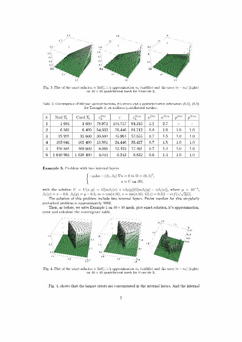
Fig. 3. Plot of the exact solution u (left), it's approximation uh (middle) and the error |u− uh| (right)on 40× 40 quadrilateral mesh for Example 2.
Tabl. 2. Convergence of bilinear approximations, it's errors and a posteriori error estimators (5.2), (5.3)for Example 2. on uniform quadrilateral meshes.
k Nod Th Card Th εDirh ε εNeu
h κDir κNeu pDir pNeu
1 1 681 1 600 78.972 104.717 94.245 1.2 2.7 - -
2 6 561 6 400 54.332 76.446 81.712 0.8 1.9 1.0 1.0
3 25 921 25 600 30.804 45.964 57.855 0.7 1.5 1.0 1.0
4 103 041 102 400 15.981 24.446 33.427 0.7 1.5 1.0 1.0
5 410 881 409 600 8.068 12.432 17.461 0.7 1.4 1.0 1.0
6 1 640 961 1 638 400 4.044 6.243 8.832 0.6 1.4 1.0 1.0
Example 3. Problem with two internal layers−µ∆u− (β1, β2).∇u = 0 in Ω = (0, 1)2,
u ≡ U on ∂Ω,
with the solution U = U(x, y) = G[mβ1(x) + vβ2(y)]G[mβ2(y) − vβ1(x)], where µ = 10−4,β1(x) = x− 0.6, β2(y) = y − 0.3, m = cos(π/6), v = sin(π/6), G(z) = 0.5[1− erf(z/
√2µ)].
The solution of this problem include two internal layers. Peclet number for this singularlyperturbed problem is approximately 8062.
Then, as before, we solve Example 1 on 40×40 mesh, plot exact solution, it's approximation,error and calculate the convergence table.
Fig. 4. Plot of the exact solution u (left), it's approximation uh (middle) and the error |u− uh| (right)on 40× 40 quadrilateral mesh for Example 3.
Fig. 4. shows that the largest errors are concentrated in the internal layers. And the internal
7
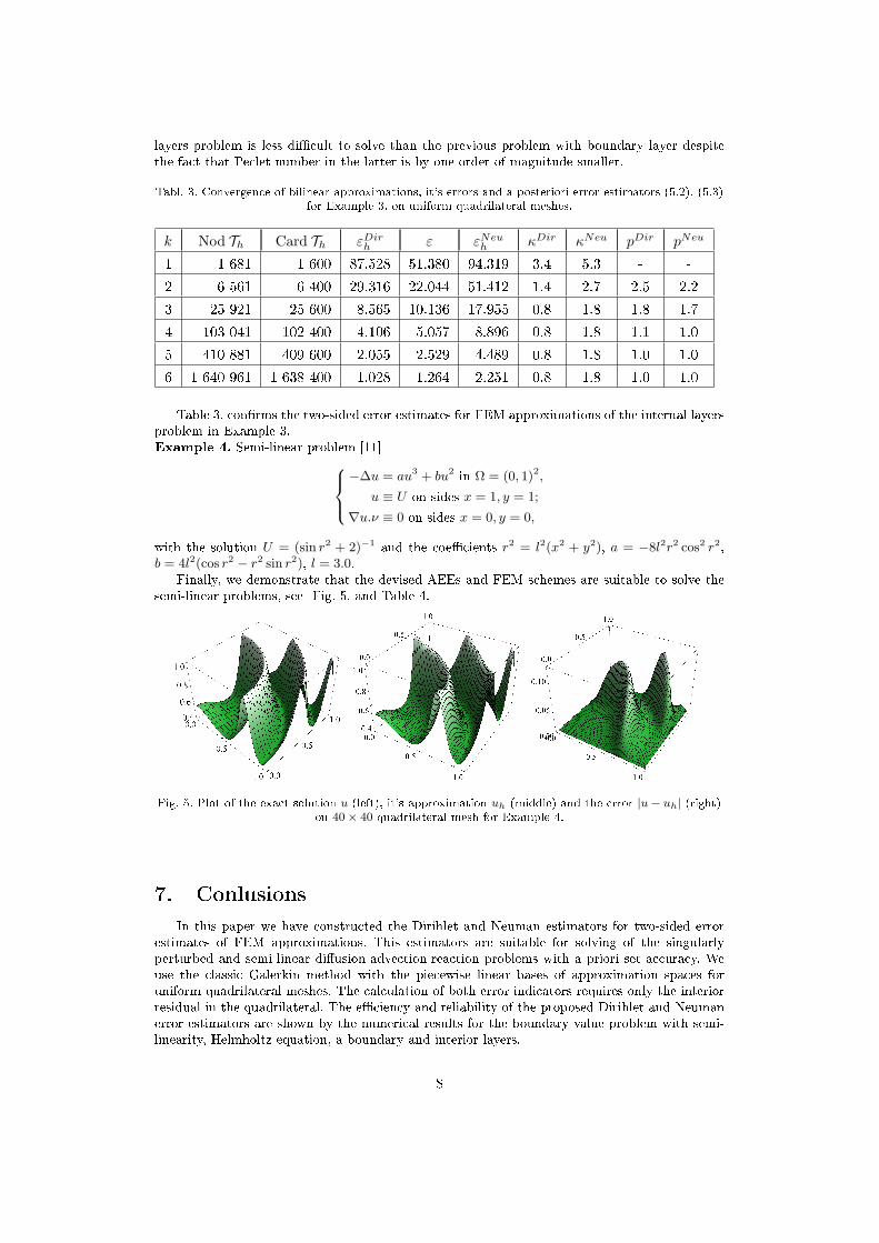
layers problem is less dicult to solve than the previous problem with boundary layer despitethe fact that Peclet number in the latter is by one order of magnitude smaller.
Tabl. 3. Convergence of bilinear approximations, it's errors and a posteriori error estimators (5.2), (5.3)for Example 3. on uniform quadrilateral meshes.
k Nod Th Card Th εDirh ε εNeu
h κDir κNeu pDir pNeu
1 1 681 1 600 87.528 51.380 94.319 3.4 5.3 - -
2 6 561 6 400 29.316 22.044 51.412 1.4 2.7 2.5 2.2
3 25 921 25 600 8.565 10.136 17.955 0.8 1.8 1.8 1.7
4 103 041 102 400 4.106 5.057 8.896 0.8 1.8 1.1 1.0
5 410 881 409 600 2.055 2.529 4.489 0.8 1.8 1.0 1.0
6 1 640 961 1 638 400 1.028 1.264 2.251 0.8 1.8 1.0 1.0
Table 3. conrms the two-sided error estimates for FEM approximations of the internal layersproblem in Example 3.Example 4. Semi-linear problem [11]
−∆u = au3 + bu2 in Ω = (0, 1)2,
u ≡ U on sides x = 1, y = 1;
∇u.ν ≡ 0 on sides x = 0, y = 0,
with the solution U = (sin r2 + 2)−1 and the coecients r2 = l2(x2 + y2), a = −8l2r2 cos2 r2,b = 4l2(cos r2 − r2 sin r2), l = 3.0.
Finally, we demonstrate that the devised AEEs and FEM schemes are suitable to solve thesemi-linear problems, see Fig. 5. and Table 4.
Fig. 5. Plot of the exact solution u (left), it's approximation uh (middle) and the error |u− uh| (right)on 40× 40 quadrilateral mesh for Example 4.
7. Conlusions
In this paper we have constructed the Dirihlet and Neuman estimators for two-sided errorestimates of FEM approximations. This estimators are suitable for solving of the singularlyperturbed and semi-linear diusion-advection-reaction problems with a priori set accuracy. Weuse the classic Galerkin method with the piecewise linear bases of approximation spaces foruniform quadrilateral meshes. The calculation of both error indicators requires only the interiorresidual in the quadrilateral. The eciency and reliability of the proposed Dirihlet and Neumanerror estimators are shown by the numerical results for the boundary value problem with semi-linearity, Helmholtz equation, a boundary and interior layers.
8
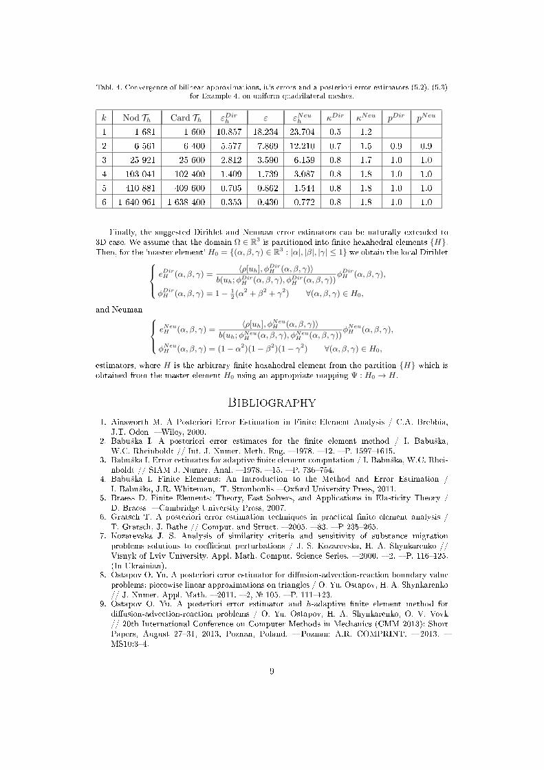
Tabl. 4. Convergence of bilinear approximations, it's errors and a posteriori error estimators (5.2), (5.3)for Example 4. on uniform quadrilateral meshes.
k Nod Th Card Th εDirh ε εNeu
h κDir κNeu pDir pNeu
1 1 681 1 600 10.857 18.234 23.704 0.5 1.2 - -
2 6 561 6 400 5.577 7.869 12.210 0.7 1.5 0.9 0.9
3 25 921 25 600 2.812 3.590 6.159 0.8 1.7 1.0 1.0
4 103 041 102 400 1.409 1.739 3.087 0.8 1.8 1.0 1.0
5 410 881 409 600 0.705 0.862 1.544 0.8 1.8 1.0 1.0
6 1 640 961 1 638 400 0.353 0.430 0.772 0.8 1.8 1.0 1.0
Finally, the suggested Dirihlet and Neuman error estimators can be naturally extended to3D case. We assume that the domain Ω ∈ R3 is partitioned into nite hexahedral elements H.Then, for the 'master element' H0 = (α, β, γ) ∈ R3 : |α|, |β|, |γ| ≤ 1 we obtain the local Dirihlet eDir
H (α, β, γ) =⟨ρ[uh], ϕ
DirH (α, β, γ)⟩
b(uh;ϕDirH (α, β, γ), ϕDir
H (α, β, γ))ϕDirH (α, β, γ),
ϕDirH (α, β, γ) = 1− 1
2(α2 + β2 + γ2) ∀(α, β, γ) ∈ H0,
and Neuman eNeuH (α, β, γ) =
⟨ρ[uh], ϕNeuH (α, β, γ)⟩
b(uh;ϕNeuH (α, β, γ), ϕNeu
H (α, β, γ))ϕNeuH (α, β, γ),
ϕNeuH (α, β, γ) = (1− α2)(1− β2)(1− γ2) ∀(α, β, γ) ∈ H0,
estimators, where H is the arbitrary nite hexahedral element from the partition H which isobtained from the master element H0 using an appropriate mapping Ψ : H0 → H.
Bibliography
1. Ainsworth M. A Posteriori Error Estimation in Finite Element Analysis / C.A. Brebbia,J.T. Oden Wiley, 2000.
2. Babuska I. A posteriori error estimates for the nite element method / I. Babuska,W.C. Rheinboldt // Int. J. Numer. Meth. Eng. 1978. 12. P. 15971615.
3. Babuska I. Error estimates for adaptive nite element computation / I. Babuska, W.C. Rhei-nboldt // SIAM J. Numer. Anal. 1978. 15. P. 736754.
4. Babuska I. Finite Elements: An Introduction to the Method and Error Estimation /I. Babuska, J.R. Whiteman, T. Strouboulis Oxford University Press, 2011.
5. Braess D. Finite Elements: Theory, Fast Solvers, and Applications in Elasticity Theory /D. Braess Cambridge University Press, 2007.
6. Gratsch T. A posteriori error estimation techniques in practical nite element analysis /T. Gratsch, J. Bathe // Comput. and Struct. 2005. 83. P 235265.
7. Kozarevska J. S. Analysis of similarity criteria and sensitivity of substance migrationproblems solutions to coecient perturbations / J. S. Kozarevska, H. A. Shynkarenko //Visnyk of Lviv University. Appl. Math. Comput. Science Series. 2000. 2. P. 116125.(In Ukrainian).
8. Ostapov O. Yu. A posteriori error estimator for diusion-advection-reaction boundary valueproblems: piecewise linear approximations on triangles / O. Yu. Ostapov, H. A. Shynkarenko// J. Numer. Appl. Math. 2011. 2, 105. P. 111123.
9. Ostapov O. Yu. A posteriori error estimator and h-adaptive nite element method fordiusion-advection-reaction problems / O. Yu. Ostapov, H. A. Shynkarenko, O. V. Vovk// 20th International Conference on Computer Methods in Mechanics (CMM 2013): ShortPapers, August 2731, 2013, Poznan, Poland. Poznan: A.R. COMPRINT. 2013. MS10:34.
9
10. Ostapov O. Yu. A posteriori error estimations for nite element approximations on quadri-lateral meshes / O. Yu. Ostapov, H. A. Shynkarenko, O. V. Vovk // VI Int. conf. named byI. I. Lyashko ¾Computational and applied mathematics¿, September 5-6, 2013. K. : TarasShevchenko National University of Kyiv, 2013. P. 3134.
11. Ostapov O. Yu. A posteriori error estimations for serendipity nite element approximationson quadrilateral meshes / O. Yu. Ostapov, H. A. Shynkarenko, O. V. Vovk // XIX Ukrainianscience conf., Modern problems of applied mathematics and computer science, Ivan FrankoNational University of Lviv, October 3-4, 2013. L. : Ivan Franko National University ofLviv, 2013. P. 1718.
12. Ostapov O. Yu. Finite element adaptive renement techniques for diusion-advection-reaction problems / O. Yu. Ostapov, H. A. Shynkarenko, O. V. Vovk // ManufacturingProcesses. Actual Problems 2013. M. Gajek, O. Hachkewych, A. Stanik-Besler eds. Poli-technika Opolska, Opole. 2013. Vol. 1. Basic science applications. P. 3146.
13. Ostapov O. Yu. H -adaptive nite element method for nonlinear problems with mixedboundary conditions / O. Yu. Ostapov, O. V. Vovk // YSC-2013, Karpenko Physico-Mechanical Institute, October 23-25, 2013. Lviv : P.P. Oschypok M.M, 2013. P. 349352.
14. Quarteroni A. Numerical Mathematics / A. Quarteroni, R. Sacco, F. Saleri // New York:Springer-Verlag, 2000.
Ivan Franko National University of Lviv, 1, Universytets'ka Str., 79000, Lviv,
Ukraine,
Opole University of Technology, 76, Proszkowska Str., 45-758, Poland, Opole
E-mail address: [email protected], [email protected]
Received 11.02.2009; revised 23.03.2009
10


