1

A scaled boundary finite element method for cyclically symmetric

two-dimensional elastic analysis

Yiqian He 1, Haitian Yang 1*, Min Xu 2, Andrew J. Deeks 3

1State Key Lab of Structural Analysis for Industrial Equipment, Dept. of Engineering Mechanics,

Dalian University of Technology, Dalian 116024, P.R. China

2School of Mathematical Sciences, Dalian University of Technology, Dalian 116024, P.R. China

3School of Engineering and Computing Sciences, Durham University,

South Road, Durham, DH1 3LE, UK

* E-mail: haitian@dlut.edu.cn; Tel.: 086-411-84708394

Abstract: A SBFEM (scaled boundary finite element method) based approach is

developed for numerical analysis of 2-D elastic systems with rotationally periodic (or

cyclic) symmetry under arbitrary load conditions. It is shown that the coefficient

matrices of the global SBFEM equations for the rotationally periodic system are block-

circulant when a symmetry-adapted reference co-ordinate system is used. Furthermore,

both the eigenproblem and stiffness matrix equation are partitioned into a series of

independent sub-problems. By solving these sub-problems via a partitioning algorithm,

solution of the whole problem can be obtained at low computing expense. Two

numerical examples are provided to illustrate the efficiency of the proposed approach.

Key words: Cyclic symmetry; scaled boundary finite element method; elastic

analysis; computational cost

2

1. Introduction

The scaled boundary finite element method (SBFEM) [1,2] is a semi-analytical

method for solving linear partial differential equations. It combines the advantages of

the FEM and BEM, and adds appealing features of its own, being particularly useful in

situations involving stress singularities and for unbounded domains [3]. The method

has been fruitfully applied to fracture problems [4-7] and foundation problems [8-11].

More recently, the meshless scaled boundary methods, including the Meshless Local

Petrov-Galerkin (MLPG) scaled boundary method [12] and Element-free Galerkin

(EFG) scaled boundary method [13], have also been developed to combine the

advantages of scaled boundary method and meshless methods. The major

computational expense of the SBFEM comes from solving a quadratic eigenproblem,

and so the computational cost rises rapidly as the number of degrees of freedom

increases [14]. Therefore one way to improve the computational efficiency of SBFEM

is to reduce the computational cost of the solution of the eigenproblem. However, most

previous work has focused on minimizing the number of degrees of freedom required

to obtain a target level of accuracy [14-17]. To the best of the authors’ knowledge, no

work has been reported which attempts to use the properties of the structure to reduce

the cost of the quadratic eigenproblem.

The present paper considers a special kind of structure, structures with cyclic

symmetry. For this kind of structure, the cyclic symmetry has been exploited in

structural FE [18,19], BE [20] and EFG [21,22] analysis. In these methods the stiffness

matrix is transformed to become block-diagonal, allowing the application of a

partitioning algorithm to reduce the computational cost of solving the whole problem.

Unlike the FE, BE and EFG methods, the stiffness matrix of the SBFEM is obtained by

solving a quadratic eigenproblem, the coefficient matrices of which are assembled in a

3

similar way to the stiffness matrix of the FE method. Therefore, in order to apply

SBFEM analysis efficiently to structures with cyclic symmetry, the major task is to

introduce an appropriate kind of partitioning algorithm into the eigenproblem. In this

paper it is demonstrated that the matrix of eigenproblem of SBFEM can be also

transferred to have the block-diagonal form using group theory, and in this way a

partitioning algorithm can be used to solve a series of independent sub-eigenproblems.

Numerical tests show that the proposed method can reduce the time consumption of the

eigenproblem dramatically, increasing the efficiency of the solution for the whole

problem as a result.

The paper commences with a brief review of the theory of rotationally periodic

symmetry and the SBFEM. The new partitioning algorithm is then developed, the

effectiveness of this procedure is then demonstrated through two examples, and the

proof for block-circulant property of the coefficient matrices is provided in the

Appendix.

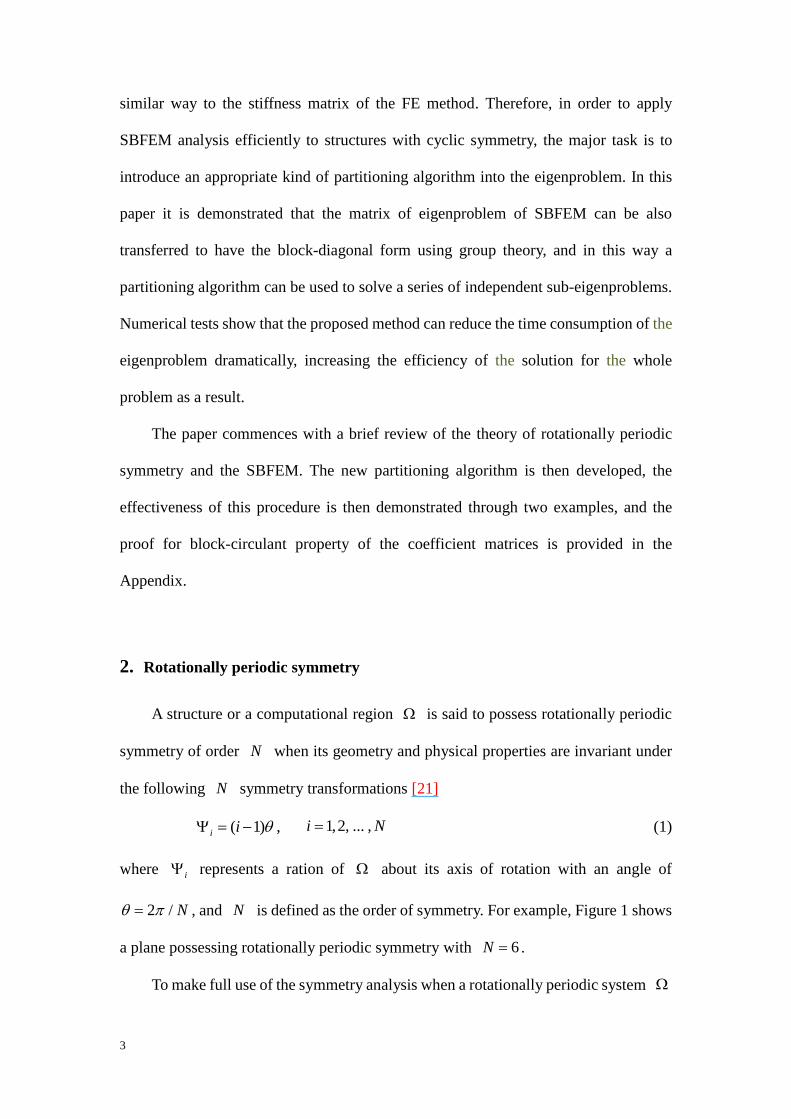
2. Rotationally periodic symmetry

A structure or a computational region is said to possess rotationally periodic

symmetry of order N when its geometry and physical properties are invariant under

the following symmetry transformations [21]

, (1)

where i represents a ration of about its axis of rotation with an angle of

2 / N , and is defined as the order of symmetry. For example, Figure 1 shows

a plane possessing rotationally periodic symmetry with 6N .

To make full use of the symmetry analysis when a rotationally periodic system

N

( 1)i i 1,2, ... ,i N

N

4

is analyzed via SBFEM, nodes are required to be arranged in a symmetric way so that

all the nodes and integration points keep the original symmetry of the system.

Figure 1 A rotationally periodic plane plate with 6.N

It is obvious that can be naturally divided into N identical parts. Arranging

these N parts in an anti-clock sequence, and designating them as i ( 1,2, ... ,i N ),

it follows that

1 2 1, :N i i (2)

Equation (2) means that i can be obtained from 1 , which is called the ‘basic

region’ and can be arbitrarily chosen from those identical parts. By setting up nodal co-

ordinates and integration points on only, one can then obtain the complete

computational model by using Equation (2). For any node or integration point in the

basic region, there are another 1N different nodes or integration points which are

located symmetrically on the other 1N symmetry regions. These N nodes

constitute a set of symmetric nodes, which is called a symmetric node orbit, and is

N

1

5

designated as AO

1 2, ,...,A NO A A A (3)

For the N nodes of , the reference co-ordinate directions of node 1A ,

which belongs to the basic region, are first defined, and then the reference co-ordinate

directions for the other symmetric nodes can be defined by using Equation (2) (see

Figure 1, for example.) It is readily seen that the six interface nodes iB ( 1,2, ... ,i N )

constitute orbit BO . Only those nodes that are located on the internal part and the ‘right’

interface of are regarded as belonging to the basic region. For example, of the two

interface nodes of the basic region in Figure 1, only 1B is regarded as belonging to

, while 2B is regarded as belonging to 2 . Assuming that the number of nodes

belonging to is denoted as m , then the total computational nodes will be N m .

3. Review of scaled boundary finite element method

Here the key equations of SBFEM will be stated, but the entire formulation will not

be repeated. The interested reader should consult references [1-3] for this.

The SBFEM introduces a normalised radial coordinate system by scaling the

domain boundary relative to a scaling centre 0 0( , )x y selected within the domain

(Figure 2). The normalised radial coordinate runs from the scaling centre towards

the boundary, and the other circumferential coordinate s specifies a distance around

the boundary from an origin on the boundary.

AO

1

1

1

6

Figure 2 Scaled boundary coordinate system

For problems of two-dimensional elasto-statics, the SBFEM obtains an approximate

solution as the weighted summation of n modes, such that the displacement at any

point within a domain is

1

( , ) ( ) i

n

i i

i

s s c

u N φ (4)

where ( )sN are the circumferential finite element (FE) shape function. The same FE

shape functions apply for all lines with a constant . ic are the modal participation

factors, iφ are the modal boundary displacements and i are the modal scaling

factors for the ‘radial’ direction. The modal boundary displacements and modal

scaling factors are determined by solving a quadratic eigenproblem which can be re-

written as a linear eigenproblem with a single coefficient matrix of double the

dimension of the original problem in the form

1 1

1

1 1

1 0 1 2 1 0

T

T

0 0φ φE E E

q qE E E E E E (5)

where the coefficient matrices 0E , 1

E and 2E are

0 1 1( s ) ( s ) dS

s T

E B D B J (6)

7

1 2 1(s) (s) dS

s T

E B DB J (7)

2 2 2(s) (s) dS

s T

E B DB J (8)

The integrals may be performed element by element over the domain boundary.

Matrices 1B and

2B are related to the polynomial shape functions used, D is the

constitutive matrix and J is the Jacobian at the boundary.

Using Φ to represent a n n matrix with domain boundary displacements for

each mode as the columns, and Q to represent the corresponding equivalent boundary

forces in equilibrium with each set of displacements, the modal participation factors for

any given set of domain boundary ( 1 ) displacements

1c Φ u (9)

where u is the nodal displacement vector and the stiffness matrix of the domain is

therefore

1K QΦ (10)

and the equilibrium requirement is reduced to

Ku P (11)

4. Properties of global coefficient matrices for cyclic symmetric structures

Consider a rotationally periodic system where the nodal displacements u can be

described by [19]

1 2, ,..., NT T T Tu u u u (12)

where the nodal vector iu belonging to the ith symmetry region is a sub-vector of u

8

with dimension 2m (since there are two degrees of freedom associated with each

node). With the degrees of freedom partitioned in this way, coefficient matrices 0

E ,

1E and

2E can be written as

11 12 1

21 22 2

1 2

N

r r r

N

r r r

r

N N NN

r r r

E E E

E E EE

E E E

,

11 12 1

21 22 2

1 2

ij ij ij

r r r m

ij ij ij

ij r r r m

r

ij ij ij

r m r m r mm

E E E

E E EE

E E E

, (13)

0,1,2r ; , 1,2,i j N

By using a symmetry-adapted reference coordinate system [21], the displacement

vector u and the nodal forces vector P can be expressed as

mu T u (14)

mP T P (15)

where

1

2

...

m

m

m

m

N

T 0

TT

0 T

, (16)

2 2

...

i

im

i

i m m

T 0

TT

0 T

, (17)

c o s ( 1 ) s i n ( 1 )

s i n ( 1 ) c o s ( 1 )i

i i

i i

T , 2 / N (18)

where N is the number of parts divided.

For each of these coordinate transformation matrices iT the following

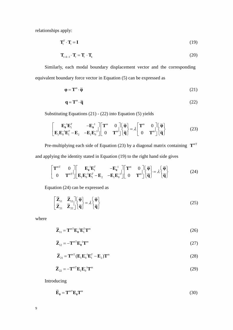
9

relationships apply:

T

i i T T I (19)

1i k i i k T T T T (20)

Similarly, each modal boundary displacement vector and the corresponding

equivalent boundary force vector in Equation (5) can be expressed as

m φ T φ (21)

m q T q (22)

Substituting Equations (21) - (22) into Equation (5) yields

1 1

1

1 1

1 0 1 2 1 0

0 0

0 0

T m m

T m m

0 0φ φE E E T T

q qE E E E E E T T (23)

Pre-multiplying each side of Equation (23) by a diagonal matrix containing TmT

and applying the identity stated in Equation (19) to the right hand side gives

1 1T

1

1 1T

1 0 1 2 1 0

0 0

0 0

Tm m

Tm m

0 0φ φE E ET T

q qE E E E E ET T (24)

Equation (24) can be expressed as

11 12

21 22

φ φZ Z

q qZ Z (25)

where

T 1

11 1

m T m 0Z T E E T (26)

T 1

12

m m 0Z T E T (27)

T 1

21 1 0 1 2( )m T m Z T E E E E T (28)

T 1

22 1 0

m m Z T E E T (29)

Introducing

Tm m0 0E T E T (30)

10

T

1 1

m mE T E T (31)

T

2 2

m mE T E T (32)

and using the identity

1 T 1m m 0 0E T E T (33)

allows Equations (26-29) to be written as

1

11 1

T 0Z E E (34)

1

12

0Z E (35)

1

2 1 1 0 1 2

T Z E E E E (36)

1

22 1 0

Z E E (37)

The coefficient matrices 0E ,

1E and 2E can be shown to be block-circulant

(refer to the appendix for the detailed proof), from which it can be proven that matrices

11Z , 12Z ,

21Z , 22Z are also block-circulant, each having the form

1 2

1

2

2 1

N

ij ij ij

N

ij ij

ij

ij

N

ij ij ij

Z Z Z

Z ZZ

Z

Z Z Z

, , 1, 2i j (38)

5. Implementation of partitioning algorithm

The parameter vector in a symmetry-adapted co-ordinate system, Au , can be defined

by

1 2, , ,T T T NT

A A A Au u u u (39)

where i

Au ( 1,2, ,i N ), belonging to the orbit AO , represents the parameters of

node iA located on the ith symmetric region.

Based on the concept of classic group theory, the vector Au can be further

11

expressed as [19]

1 2

1

, , ,N

T T

Aj Aj i N Aj

i

u u e e e e u (40)

where

1 1 , 1 , , 1T

Ne

2 1 22 cos ,cos , ,cosT

i NN i i i e

2 1 1 22 sin ,sin , ,sinT

i NN i i i e

1 , , 1 2i N , 1 1,2, ,k k k N

1, 1,1, , 1T

N N e (when N is even) (41)

Here 1 2, , ,T

Ne e e represents a group of complete symmetrized orthogonal unit

vectors, 1 2N is the largest integer which does not exceed 1 2N , i

Aju

( 1,2, ,i N ) is the expansion coefficient of the parameter vector Au corresponding

to ie , subscript j refers to j th direction ( 1,2j ).

Therefore

mu E u (42)

where

[ ]m m T

rs E e I (43)

mI is unit matrices of 2m dimensions. rse is the s th element of the basis re , and

u can be called global generalized parameter vector.

Utilizing Equation (42) and Equation (14), and multiplying mTE on the left-hand

sides of Equation (11)

Ku P (44)

12

where

T T Tm m m m m m K E KE E T KT E (45)

T Tm m m mP E T PT E (46)

Similarly, for modal boundary displacement vectors and the corresponding

equivalent boundary force vector one has

mφ E φ (47)

mq E q (48)

Utilizing Equations (47) and (48), the eigenproblem of Equations (25) can be

expressed as

11 12

21 22

φ φZ Z

Z Z q q (49)

where

m T m

i j i jZ E Z E, , 1, 2i j (50)

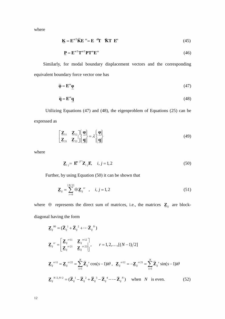
Further, by using Equation (50) it can be shown that

[ 2]

0

Nrr

ij ij

r

Z Z , , 1, 2i j (51)

where represents the direct sum of matrices, i.e., the matrices ijZ are block-

diagonal having the form

00 1 2( )N

ij ij ij ij Z Z Z Z

11 12

21 22

rr rr

ij ijrr

ij rr rr

ij ij

Z ZZ

Z Z, 1,2, ,[( 1) 2]r N

11 22

1

cos( 1)N

rr rr s

ij ij ij

s

s i

Z Z Z , 12 21

1

sin( 1)N

rr rr s

ij ij ij

s

s i

Z Z Z

/2, /2 1 2 3 4( )N N N

ij ij ij ij ij ij Z Z Z Z Z Z when N is even. (52)

13

Based on Equation (52), it is clear that the eigenproblem of Equation (49) can be

naturally partitioned into [ 2 2]N decoupled sub-eigenproblems

11 12

21 22

r rrr rr

rr rr r r

φ φZ Z

Z Z q q, 0,1,2, , 2r N (53)

Therefore, instead of solving the original eigenproblem Equation (5), now one

only needs to solve a series of independent small sub-eigenproblems, as shown in

Equation (53). Obviously the partitioning of the original eigenproblem into a series of

small sub-problems leads to significantly higher efficiency of computation, which will

be demonstrated by the numerical examples given in the next section.

Using Φ to represent a n n matrix assembling each displacement mode

matrix iΦ solved by the series of sub-eigenproblems in Equation (53), and Q to

represent the matrix assembling the corresponding equivalent force matrices iQ , Φ

and Q can be expressed as

0

1

/2N

Φ

ΦΦ

Φ

0

1

/2

...

N

Q

QQ

Q

(54)

Multiplying Q and 1Φ together yields

* 1K QΦ (55)

Noting that

m mΦ T E Φ (56)

m mQ T E Q (57)

Equation (10) can be written

14

1

1 1

1

*

( )

mT mT m m

mT mT m m

mT mT m m m m m m

K E T KT E

E T QΦ T E

E T T E QΦ T E T E

QΦ

K

(58)

As both matrices Q and Φ are block-diagonal, it has been shown that the

matrix K is also block-diagonal, having the same form as the eigenproblem in

Equation (53). Similarly, instead of solving the original Equation (11), now one only

needs to solve a series of independent small sub-problems.

The block-diagonal nature of Q , Φ and K is only preserved if prescribed

displacement boundary conditions are also cyclically symmetric. However, there is no

requirement that the external force terms are cyclically symmetric, as cyclic symmetry

of P is not assumed in the derivation of K . Transformation of these terms occurs

through Equation (46), allowing the solution of Equation (44).

6. Numerical examples

Example 1 - A square plate

The first example refers to a square plate subjected to tension, as shown in Figure

3, where the geometry, physical properties, and constraint conditions are invariant

under 4N symmetry transformations. The length of square side is 2l m , plane

stress conditions were assumed with Young’s Modulus 3 21 10 /E N m and Possion’s

ratio 0.25v . The distributed force is 1 /P N m and the displacement boundary

conditions are fixed to zero at corresponding position as shown in Figure 3. Rather than

using the conventional SBFEM to model the whole domain to solve this problem, here

15

the proposed partitioning algorithm is used. As shown in Figure 4, uniform nodes are

introduced along this edge, the nodes spacing is specified as ds .

All the calculation in this paper is conducted by PC with I5-2410M 2.3GHz CPU

and 4GB RAM.

To compare the precision of the proposed method, Table 1 provides a comparison

of the new SBFEM method and the ANSYS Finite Element Program. The SBFEM uses

160 nodes, while ANSYS uses 4961 nodes and 1600 8-node-quadrangle finite elements.

The displacements at the four corner points of the square domain were calculated. Good

agreement between proposed method and ANSYS is shown in Table 1, in which the

maximum difference is 0.65%.

Table 2 shows the comparison of CPU times between the conventional SBFEM

and the proposed SBFEM with partitioning algorithm. Two different node densities are

used, and the CPU time needed to solving the eigenproblem, the stiffness matrix

equation and the entire problem are compared. The results show that as the proposed

partitioning algorithm increases the efficiency of the SBFEM considerably. In particular,

the computing efficiency for the solution of the eigenproblem can be increased 6.8 and

6.9 times.

Table 2 Comparison of CPU time

Solution method

EFG-SBM without

partitioning

Time t1(s)

Partitioning algorithm

Time t2(s) Ratio t1/t2

160

nodes

Solution of eigenproblem 3.7510 0.5480 6.84

Solution of K equation 0.0050 0.0020 2.50

Entire procedure 5.0480 1.9820 2.54

16

200

nodes

Solution of eigenproblem 7.1070 1.0270 6.92

Solution of K equation 0.0110 0.0020 5.50

Entire procedure 9.0740 3.1590 2.87

Example 2 - A dodecagon plate

Consider a dodecagon plate subjected to a distributed force 1 /p N m along

one side, as shown in Figure 5, where 1R m and the length of each side is represented

by l . There are twelve hinged supports following cyclic symmetry along the outer

boundaries.

It is readily seen that geometry, physical properties and constraint conditions are

invariant under the 12N symmetry transformations. Plane stress conditions are

assumed with Young’s modulus 22000N/mE and Poisson’s ratio 0.25 . The

distribution of uniform nodes with spacing ds on the boundary of the basic region is

shown in Figure 6.

Figure 6 Distribution of nodes for the basic region 1 for a dodecagon plate

17

The above problem is solved via the proposed SBFEM with partitioning algorithm,

and the accuracy is verified by comparison with numerical results obtained using

ANSYS. The SBFEM uses 600 nodes, while ANSYS uses 4469 nodes and 1469 8-

node-quadrangle finite elements.

Table 3 shows the computed displacement results. Good agreement between the

proposed method and ANSYS can be found.

Table 3 Comparison of displacement results

Co-ordinate

(x, y)

Point A

(0.2500,0.9330)

Point B

(0.6830,0.6830)

Point C

( 0.9330,0.2500)

Point D

(0.2500, 0.9330)

Displacement

(×10-4m) u v u v u v u v

ANSYS(FEM) 1.2040 1.5506 4.3595 4.3595 0.8487 0.6059 0.4806 0.8935

Partitioning

algorithm 1.1997 1.5596 4.3518 4.3518 0.8475 0.6074 0.4810 0.8927

Difference (%) 0.3571 0.5804 0.1766 0.1766 0.1414 0.2476 0.0832 0.0895

Table 4 shows the comparison of CPU times between the conventional SBFEM

and the proposed SBFEM with partitioning algorithm. The results show that when the

proposed partitioning algorithm is used, both the solution of eigenproblem and the

solution of stiffness matrix K equation are accelerated significantly, reducing the

total time required to solve the problem significantly. Figure 7 shows the variation of

CPU time with DOF, comparing the proposed and conventional SBFEM approaches.

The ability of proposed algorithm to increase computational efficiency is clearly

demonstrated.

18

Table 4 Comparison of CPU time

Solution method

EFG-SBM without

partitioning

Time t1(s)

Partitioning

algorithm

Time t2(s)

Ratio t1/t2

240 nodes

Solution of eigenproblem 9.9180 0.2540 39.04

Solution of K equation 0.0300 0.0020 15.00

Entire procedure 12.6350 3.3160 3.81

480 nodes

Solution of eigenproblem 85.147 1.8000 47.30

Solution of K equation 0.2630 0.0110 23.90

Entire procedure 100.3620 17.9330 5.59

600 nodes

Solution of eigenproblem 179.7520 3.679 48.85

Solution of K equation 0.4300 0.0170 25.29

Entire procedure 209.1830 37.1470 5.63

19

(a) Solution of eigenproblem

(b) Entire procedure

Figure 8 The variation of CPU time with DOF comparing proposed and conventional SBFEM

7. Concluding remarks

Cyclic symmetry has been utilized in SBFEM analysis for rotationally periodic

systems. By adopting a symmetry adapted reference system, the coefficient matrices

and the eigenproblem matrix of the SBFEM equation can be transformed into a block-

circulant form, and a partitioning algorithm has been proposed. The major advantages

of exploitation of cyclic symmetry in the SBFEM analysis include the following:

1. Only 1/N part of coefficient matrix needs to be formed.

2. By the transformation, only a series of small sub-eigenproblems and stiffness

20

matrix equations require solving independently, instead of the whole problem. Thus,

the computational efficiency is significantly increased.

3. Even higher computing efficiency can be expected in the future, as the proposed

partitioning algorithm facilitates parallel processing.

The formulation presented is restricted to structures with cyclic symmetry of both

geometry and constraints. The authors are currently attempting to extend the approach

to situations where only the geometry possesses cyclic symmetry.

Acknowledgements

The research leading to this paper is supported by NSF [10421002, 10772035, 10721062, 11072043,

11202046], and NKBRSF [2005CB321704, 2010CB832703], the China Postdoctoral Science

Foundation [2012M520617], and the Fundamental Research Funds for the Central Universities

[DUT11RC(3)33]. .

References

[1] J.P. Wolf, C. Song, Finite-Element Modelling of Unbounded Media. John Wiley and Sons,

Chichester, 1996.

[2] J.P. Wolf, The Scaled Boundary Finite Element Method. John Wiley and Sons, Chichester, 2003.

[3] A.J. Deeks, J.P. Wolf, A virtual work derivation of the scaled boundary finite-element method

for elastostatics, Comput. Mech. 28(2002) 489-504.

[4] E.T. Ooi, Z.J. Yang, Modelling crack propagation inreinforced concrete using a hybrid finite

element-scaled boundary finite element method, Eng. Frac. Mech. 78(2010) 252-273.

[5] E.T. Ooi, Z.J. Yang, A hybrid finite element-scaled boundary finite element method for crack

propagation modelling, Comput. Meth. App. Mech. Eng. 199(2010) 1178-1192.

[6] E.T. Ooi, Z.J. Yang, Modelling dynamic crack propagation using the scaled boundary finite

element method, Int. J. Numer. Meth. Eng. 88(2011) 329-349.

21

[7] Z.J. Yang, A.J. Deeks, H. Hao, Transient dynamic fracture analysis using scaled boundary finite

element method: a frequency domain approach, Eng. Frac. Mech. 74(2007) 669-687.

[8] A.J. Deeks, J.P. Wolf, Semi-analytical elastostatic analysis of two-dimensional unbounded

domains, Int. J. Numer. Analy. Meth. Geomech. 26(2002) 1031-1057.

[9] J.P. Doherty, A.J. Deeks, Scaled boundary finite-element analysis of a non-homogeneous half-

space, Int. J. Numer. Meth. Eng. 57(2003) 955-973.

[10] J.P. Doherty, A.J. Deeks, Scaled boundary finite-element analysis of a non-homogeneous

axisymmetric domain subjected to general loading, Int. J. Numer. Analy. Meth. Geomech.

27(2003) 813-835.

[11] J.P. Doherty, A.J. Deeks, Elastic response of circular footings embedded in a non-homogeneous

half-space, Geotech. 53(2003) 703-714.

[12] A.J. Deeks, C.E. Augarde, A meshless local Petrov-Galerkin scaled boundary method, Comput.

Mech. 36(2005) 159–170.

[13] Y.Q. He, H.T. Yang, A.J. Deeks, An Element-free Galerkin (EFG) scaled boundary method,

Fin. Elem. Analy. Des. 62(2012) 28-36.

[14] A.J. Deeks, J.P. Wolf, An h-hierarchical adaptive procedure for the scaled boundary finite-

element method, Int. J. Numer. Meth. Eng. 54(2002) 585-605.

[15] T.H. Vu, A.J. TH, Deeks, AJ. (2006). Use of higher order shape functions in the scaled

boundary finite element method, Int. J. Numer. Meth. Eng.. International Journal for Numerical

Methods in Engineering, 65(2006) 10):1714-1733.

[16] T.H. Vu, A.J. TH, Deeks, AJ. (2008). A p-hierarchical adaptive procedure for the scaled

boundary finite element method, Int. J. Numer. Meth. Eng.International Journal for Numerical

Methods in Engineering, 73(2008) :47-70.

[17] T.H. Vu, A.J. TH, Deeks, AJ. (2008). A p-adaptive scaled boundary finite element method

based on maximization of the error decrease rate, Comput. Mech.. Computational Mechanics,

41 (2008) :441-455.

[18] W.X.18 Zhong, C.H. Qiu, Analysis of symmetric or partially symmetric structures. Comput.

Meth. App. Mech. Eng. 38(1983) 1-18.

[19] L.19 Liu, H.T. Yang, FE analysis based on Lagrange multipliers method and group theory for

22

structures of cyclic symmetry under arbitrary displacement boundary conditions, Chinese J.

Comput. Mech. 21(2004) 425-429.

[20] G.F.20 Wu, H.T. Yang, The use of cyclic symmetry in two-dimensional elastic stress analysis

by BEM. Int. J. Solids Struct. 31(1994) 279-290.

[21] H.T.21 Yang, L. Liu, Z. Han, The use of cyclic symmetry in two-dimensional elastic analysis

by the element-free Galerkin method, Commun. Numer. Meth. Eng. 21(2005) 83-95.

[22] L.22 Liu, H.T. Yang, A paralleled element-free Galerkin analysis for structures with cyclic

symmetry, Eng. with Comput. 23(2007) 137–144.

23

Appendix: Proof for block-circulant property

Based on SBFEM theory, the relevant coefficient matrices containing the shape

function are

1 1( ) ( ) ( )s s s B b N (A1)

2 2

,( ) ( ) ( ) ss s s B b N (A2)

where

T

, ,1

, ,

( ) 0 ( )( )

0 ( ) ( )

s s s s

s s s s

y s x ss

x s y s

b (A3)

T

2( ) 0 ( )

( )0 ( ) ( )

y s x ss

x s y s

b (A4)

In a symmetric system, points belonging to the same orbit follow

cos sin,

sin cos

i t i

j t j t

t t

t t

x T x T (A5)

and

cos sin

sin cos

i t i i

j j j

i t i i

j j j

x x t y t

y x t y t

(A6)

therefore

cos sin

sin cos

i t i t i i t i i i

j j j j j j j

i i

j j

i t i t i i t i i i

j j j j j j j

i i

j j

x x x x y x yt t

s x s y s s s

y y x y y x yt t

s x s y s s s

(A7)

The scaled boundary and Cartesian coordinate systems are related by the scaling

equations

0 ( )sx x x s (A8)

0 ( )sy y y s (A9)

24

As the coefficient matrix is calculated on the boundary 1 , so

,( )s s

xx s

s

(A10)

,( )s s

yy s

s

(A11)

therefore

( ) ( )p p tq q

s s x x

N N (A12)

, ,( ) ( )p p tq q

s ss s

x x

N N (A13)

1

sin cos 0 (cos sin )

( )

0 (cos sin ) sin cos

p tq

i i i i

i i i i

x y x yt t t t

s s s ss

x y x yt t t t

s s s s

xb

(A14)

2

sin cos 0 (cos sin )

( )

0 (cos sin ) sin cos

p tq

i i i i

i i i i

x y x yt t t t

s s s ss

x y x yt t t t

s s s s

xb

(A15)

and

0

( ) 0

( ) 0 ( )

0 ( )

0 ( ) ( )

( ) ( )

pq

k

k

i i

i ik

k

ik i i

i ik k

k k

yN s

sy xN s N s

xs sN s

sx yN s N s

x ys sN s N s

s s

xE D

(A16)

25

0cos( ) sin( )

sin( ) cos( )

sin cos ( ) 0 (cos sin ) ( )

0 (cos sin ) ( ) sin cos ( )

p tq

T

ik

i i i ii i

i i i ii i

t t

t t

x y x yt t N s t t N s

s s s s

x y x yt t N s t t N s

s s s s

xα E α

sin cos ( ) 0

cos( ) sin( )0 (cos sin ) ( )

sin( ) cos( )

(cos sin ) ( ) sin cos ( )

k ik

k kk

k k k kk k

x yt t N s

s s

t tx yt t N s

t ts s

x y x yt t N s t t N s

s s s s

D

(A17)

It follows that 0 0

p p tq q

T

ik ik

x xE α E α

and therefore

T T

0 0p p tq q

ik ik

m n m t n t x x

T E T T E T (A18)

T T ,

0 0

mn m t n t

m n m t n t

T E T T E T (A19)

,

0 0

mn m t n t E E (A20)

Similarly, ,

1 1

mn m t n t E E and ,

2 2

mn m t n t E E can also be proved.