A sensitivity study of high-resolution regionalclimate simulations to three land surfacemodels over the western United StatesFeng Chen1,2, Changhai Liu2, Jimy Dudhia2, and Ming Chen2

1Zhejiang Institute of Meteorological Sciences, Hangzhou, China, 2National Center for Atmospheric Research, Boulder,Colorado, USA

Abstract The Weather Research Forecasting model is applied for convection-permitting regional climatesimulations over the western United States using three different land surface schemes (Noah, NoahMP, andCLM). Simulated precipitation, temperature, and snow water equivalent (SWE) are evaluated by comparingagainst Snow Telemetry (SNOTEL) and Parameter-elevation Regressions on Independent Slopes Model(PRISM) observations. The results show that all simulations realistically reproduce the spatial and temporalvariability of precipitation without significant sensitivity to the choice of land surface scheme, even thoughthey tend to overestimate themagnitude of the SNOTEL data by about 15%. Comparing the bias with respectto the SNOTEL data, CLM is superior in 2 m maximum temperature, while NoahMP is most skillful in 2 mminimum temperature. Land surface parameterizations have high impacts on snowpack simulations.The SWE peaks too early with an unrealistically low value and also ablates too fast in Noah. NoahMPimproves the SWE estimate to some extent, and CLM best represents the observations. Overall, CLM andNoahMP outperform Noah. Further analysis reveals that these differences are largely attributed todistinct rainfall-snowfall partitioning, snow albedo treatment, vegetation treatment, and surface data inthese schemes.

1. Introduction

It is well known that the land surface process plays a key role in regulating regional climate. Land surface physicsinvolve the exchanges of momentum, energy, and mass (water, aerosols, and other important chemicalconstituents) between the land surface and overlying atmosphere, which can affect the regional climate both ontime scales of seconds to hours (exchanges in rapid biophysical and biogeochemical processes) and days toseasons (exchanges in the storage of soil moisture, snowpack, carbon allocation, and vegetation phenology).

Snow processes are an important component of surface physics. It affects the regional climate through itsinfluence on the partitioning of incident radiation and the dynamics of moisture storage in snow-coveredmountainous regions [Groisman et al., 1994]. The high albedo of the snowpack results in a more reflectiveplanet and reduces the net-absorbed solar radiation on the ground, which will ultimately influence thethermodynamic processes [Cess et al., 1991; Cohen and Entekhabi, 2001]. Water storage in the snowpackduring the cold season and its release during the melting season has an important impact on hydroclimaticprocesses and water resource management [Grant and Kahan, 1974]. In the western U.S., for instance, snowaccounts for 50–70% of the annual precipitation [Serreze et al., 1999], and about 85% of the annualstreamflow comes from snowmelt runoff [Grant and Kahan, 1974]. Recent research has shown that snowpackis especially sensitive to climate change with the most pronounced decrease at low and middle elevations[McCabe and Clark, 2005], and the combination of increased temperature and weak to no trend in snowfallmay produce a drought condition over the next 50 years in the western U.S. [Hoerling and Eischeid, 2006;Seager et al., 2007; Intergovernmental Panel on Climate Change, 2007; Collins et al., 2013]. Therefore, improvingthe capability of snowpack prediction in numerical models is crucial to the comprehensive water resourcemanagement. Additionally, snowpack prediction in land surface models (LSMs) is highly related toprecipitation, temperature, and physical-dynamical options in the model (including numerical methods,physical processes, parameters, etc.). More precipitation would directly increase the snowfall (when thetemperature is low) at surface, and increase the accumulation of snowpack. Low temperature would slowdown the snow melting process and increase the refreezing process, eventually leading to the increase of

CHEN ET AL. ©2014. American Geophysical Union. All Rights Reserved. 7271

PUBLICATIONSJournal of Geophysical Research: Atmospheres

RESEARCH ARTICLE10.1002/2014JD021827

Key Points:• All simulations realistically reproduceprecipitation and temperature

• Temperature and SWE are moresensitive than precipitation to thechoice of LSMs

• Noah produces low and early SWEpeak; NoahMP and CLM improve it

Correspondence to:F. Chen,fchen_zj@163.com

Citation:Chen, F., C. Liu, J. Dudhia, and M. Chen(2014), A sensitivity study of high-resolution regional climate simulations tothree land surface models over thewestern United States, J. Geophys. Res.Atmos., 119, 7271–7291, doi:10.1002/2014JD021827.

Received 31 MAR 2014Accepted 31 MAY 2014Accepted article online 9 JUN 2014Published online 26 JUN 2014

snowpack accumulation. Therefore, precipitation and temperature might be as important as the snowprocess itself and play a key role in snowpack prediction.

Recent efforts aimed at better understanding and more accurately predicting snow mass have providedimportant insights into snow processes [Sun et al., 1999; Leung and Qian, 2003; Liston, 2004; Jin and Miller,2007; Rauscher et al., 2008;Wang and Zeng, 2009; Livneh et al., 2010;Wang et al., 2010; Barlage et al., 2010]. Forexample, Leung and Qian [2003] improved snowpack simulation by using higher spatial resolution; Liston[2004] described subgrid snow cover heterogeneities in regional and global models; Wang and Zeng [2009]improved the treatment of the vertical snow burial fraction over short vegetation in the National Center forAtmospheric Research Community Land Model 3 (NCAR CLM3), and so on. However, there still exist largeuncertainties in the prediction of snowfall and snowpack in complex terrain. For instance, precipitation wasoverestimated by 30–72% with NCAR Mesoscale Model (MM5) and National Centers for EnvironmentalPrediction Regional Spectral Model in Leung et al. [2003], but precipitation was almost doubled that ofobservation with Weather Research and Forecasting (WRF) in Jin et al. [2010]. The snowpack characteristicssimulated by some land surface models (such as Noah LSM and Noaa RUC) exhibited a significantly lowand early snow water equivalent (SWE) peak and a too early end of the snow period [Jin and Wen, 2012]. Suchkinds of model bias could come from oversimplified snow physics, as well as atmospheric forcing, modelresolution, model structure, and so on. As such, land surface models with sophisticated snow processes havebeen developed and coupled with global climate models and regional models. The Weather Research andForecasting (WRF) model, a state-of-the-art regional weather and climate model, has been recently coupled withtwo advanced land surface models, i.e., the community Noah land surface model with multiphysicsparameterization options (NoahMP) [Niu et al., 2011], and the Community Land Model (CLM) [Jin and Wen, 2012].Note that NoahMP was previously tested offline [Yang et al., 2011], and a previous version of CLM (version 3.5)coupled with WRF was tested [Subin et al., 2011; Lu and Kueppers, 2012]. The version of CLM used here (version 4)was also tested offline [Lawrence et al., 2011]. However, an evaluation of their performance in a large domainand over a long time period is still lacking. Moreover, their usage in high-resolution (e.g., convection-permitting)models has not been tested before. Additionally, more physical options are available in WRF now. Applicationof these new schemes may interact with LSMs and help in improving the simulations.

The goal of this paper is to evaluate and compare the skill of three LSMs (Noah, NoahMP, and CLM) inrepresenting precipitation, temperature, and snowpack over the western United States. The results willprovide useful information about the relative performance of these LSMs for the regional climate communityand suggestions on what physics processes may require further improvement for LSM developers. The studyregion is characterized by complex terrain, abundant snowfall, and significant seasonal snowpack in all of themountain ranges. Also, this domain has a relatively dense snow telemetry network which facilitates theverification of model results. All of these aforementioned features make the western U.S. an ideal location fortesting LSMs. Other important features of the present study include the multimonth integration spanningboth the early accumulation and subsequent ablation of snowpack and the use of a convection-allowingregional climate model with a large computational domain, unlike previous fine grid but small-domain modelingor large domain but coarse-grid regional climate simulations. It should be pointed out that fine-grid spacing(e.g., < 6 km) is critical to an adequate depiction of mesoscale topography and associated precipitation andsnowpack modulations [Leung and Qian, 2003; Ikeda et al., 2010; Rasmussen et al., 2011] because areas of highelevation need to be resolved. An additional benefit of high resolution is the exclusion of convectiveparameterization and thus its complication in the interpretation of model results. All of these particular strengthsenable us to draw rather robust conclusions of the advantages and weaknesses of each tested LSM.

The paper is organized as follows. Section 2 introduces the model configuration, land surface schemes to betested, and validation data. Model results and their evaluations with observations are reported in section 3.Section 4 discusses responsible factors for the differences of model results associated with the LSM selection.Finally, conclusions are presented in section 5.

2. Model Description and Verification Data2.1. Numeric Model and Experiments

The Weather Research and Forecasting (WRF) model [Skamarock et al., 2008] version 3.5.1 (http://www2.mmm.ucar.edu/wrf/users) is applied to the western U.S. (Figure 1). The computational domain has 626×552 grid

Journal of Geophysical Research: Atmospheres 10.1002/2014JD021827

CHEN ET AL. ©2014. American Geophysical Union. All Rights Reserved. 7272

points with 4 km grid spacing in the horizontal and 51 stretched vertical levels topped at 50 hPa. The employedphysics parameterizations include the Thompson cloud microphysics scheme [Thompson et al., 2008], the newRapid Radiative Transfer Model shortwave and longwave radiation scheme [Iacono et al., 2008], the YonseiUniversity planetary boundary layer scheme [Hong and Pan, 1996], and the revised Monin-Obukhov surface layerscheme [Jimenez et al., 2012], as well as the land surface schemes being tested. This suite of physicsparameterizations is selectedmainly on the basis of previous sensitivity investigations of the simulation ofmultiplemonths of precipitation to various physical parameterizations, especially microphysics [Liu et al., 2011].

The Climate Forecast System Reanalysis (CFSR) [Saha et al., 2010] is used to provide initial and lateral boundaryconditions. This data set has a 6-hourly temporal resolution and a 0.5° spatial resolution. The model integration isconducted over a 9 month period from 1 October 2007 through 30 June 2008, covering both snow accumulatingand most of the melting period. A total of three numerical experiments are performed with three different landsurface schemes, respectively, referred to as Noah, NoahMP, and CLM. All simulations used initial CFSR soiltemperature and moisture on 1 October 2007. No spin-up was used, but we expect the initial soil moisture not tohave a large effect on precipitation and developing snow pack, since the winter precipitation/snowfall issignificantly modulated by the upstream inflow from the ocean and underlying topography in our study domain.

2.2. Land Surface Models

This study focused on three LSMs available in the WRF model, namely, Noah, NoahMP, and CLM. The defaultmodel parameters in these schemes are used. Table 1 compares several important features between theseLSMs, including vegetation types, soil levels, snow layers, canopy separation, and canopy radiative transfer.

Figure 1. Model domain and geographical distribution of the SNOTEL stations (black dots). The shading represents terrain(m), and blue rectangles are subregions covering major mountain ranges.

Table 1. Comparison of the Noah, NoahMP, and CLM Land Surface Schemes in WRF

Scheme Vegetation Types Per Cell Soil Levels Snow Layers Separate Canopy Canopy Radiation Transfer

Noah 1 4 1 (blend with soil) No NoNoahMP 1 4 Up to 3 Yes Two streamCLM up to 4 10 Up to 5 Yes Two streamScheme Vegetation interception Under canopy heat flux Water transfer between layers, refreeze Snow density Vertical burialNoah Liquid No No Fixed NoNoahMP Liquid+ ice M-O similarity Yes Variable NoCLM Liquid+ ice M-O similarity Yes Variable Yes

Journal of Geophysical Research: Atmospheres 10.1002/2014JD021827

CHEN ET AL. ©2014. American Geophysical Union. All Rights Reserved. 7273

The Noah land surface scheme is an olderimplemented scheme. It has four soil layerswith a total depth of 2 m and a combinedsurface layer of vegetation and soil surface.Detailed descriptions can be found in Korenet al. [1999], Chen and Dudhia [2001], andEk et al. [2003]. Only a brief summaryrelated to snow processes is given here. TheSWE is calculated as the residual of snowfallminus the sum of snowmelt andsublimation. Snow melting occurs whenthe temperature is higher than 0°C, andsnow freezing occurs when thetemperature is lower than 0°C. No canopyinterception of ice, water transfer betweenlayers, and refreezing are considered. Dueto such a layer structure and oversimplifiedsnow physics, the Noah scheme is known tohave biases in simulating runoff andsnowmelt [Bowling et al., 2003; Slater et al.,2007; Jin and Wen, 2012].

The NoahMP scheme augments theconceptual realism in biophysical andhydrological processes based on the Noahscheme and introduces a framework formultiple options to parameterize selectedprocesses. The vegetation canopy layer is

separated from the combined surface layer, and the two-stream radiation transfer scheme is used to calculatethe canopy radiation transfer. A Ball-Berry type stomatal resistance scheme is chosen to consider thedifference of sunlit and shaded leaves, and a short-term dynamic vegetation model and a frozen soil schemeare coupled. Especially, a physically based three-layer snow model is implemented. This LSM allows for bothliquid water and ice to be present on the vegetation canopy and considers the melting and refreezing in thecanopy. The snow layer on the ground is divided based on the snow depth; snow melting/freezing occurswhen the temperature is higher/lower than 0°C, and the water transfer between layers is considered. Inaddition, the scheme enables the choice of multiple, alternative options for each physical process. Detaileddescriptions can be found in Niu et al. [2011] and Yang et al. [2011]. Due to these improved physics, itperforms better in land surface modeling than Noah [Niu et al., 2011; Yang et al., 2011].

The CLM scheme is newly coupled into WRF in an effort to improve simulations of land surface processes. Itconsiders the vegetation, soil, and snow separately. A subgrid mechanism is considered in CLM, and up to 4of 16 plant functional types are allowed in one grid cell, each type characterized by distinct physiologicalparameters. Ten soil layers with a depth of 3.43 m and up to five snow layers are used to calculate thetemperature and water content in each layer. The canopy interception of snow is a function of the leaf andstem area indexes, whereas the leaf and stem area indexes are adjusted by the vertical burial fraction due tosnow. The snow compressing, melting and refreezing, and water transfer between layers are also considered.Additionally, a new snow aging parameterization [Flanner and Zender, 2006] and a treatment of aerosoldeposition [Lawrence et al., 2011] are also included in the model, which may affect the simulation of snowthickness and albedo. A detailed description can be found in Oleson et al. [2010]. Although Subin et al. [2011]showed some improvements in temperature and near-surface humidity simulation using CLM as comparedto using Noah, there were large biases in both models for daily minimum temperature and orographicprecipitation. Large biases are also found in CLM simulation of SWE, which are probably related tooverestimated precipitation. Lu and Kueppers [2012] showed that warm biases existed over the entire domainpossibly due to inappropriate atmospheric radiation parameterization, even after improving therepresentation of vegetation and irrigation. Jin and Wen [2012] showed a large improvement in the SWE

Figure 2. Taylor diagram comparing simulations with observation.(Red for Noah, green for NoahMP, and blue for CLM. PREC for preci-pitation, Tmax for 2 m maximum temperature, Tmin for 2 m minimumtemperature, Tmean for 2 m mean temperature, SWE for snow waterequivalent, SWEPK for snow water equivalent peak value, and SWEPTfor snow water equivalent peak time.) The normalized standardizeddeviation represents the ratio of the simulated and observedstandardized variances. The closer to the reference point, the highercorrelation and less difference in variances. The percentage bias isindicated by different size of symbols, and the best one is highlightwith the square of its label.

Journal of Geophysical Research: Atmospheres 10.1002/2014JD021827

CHEN ET AL. ©2014. American Geophysical Union. All Rights Reserved. 7274

simulation, which agrees well with observations when using CLM. The above three studies use differentcombinations of physical schemes in WRF, and use CLM3.5 rather than CLM4. Therefore, more evaluationswith different resolutions and atmospheric schemes are needed, and the use of the updated CLM4 and aconvection-resolving resolution might be helpful to improve the simulation.

2.3. Verification Data

Snow Telemetry (SNOTEL) observed data [Serreze et al., 1999] that include daily precipitation, 2 m heightmaximum/minimum/average temperature, and SWE are used here for evaluation. Observations are takenfrom 637 selected SNOTEL stations (black dots in Figure 1), all of which are typically located at elevationsbetween 1200 and 3200 m above mean sea level. Weighing-type gauges often underestimate snowfall dueto wind [Serreze et al., 2001; Rasmussen et al., 2001; Tian et al., 2007]. However, the wind speed is typically lessthan 2 m s�1, for which an undercatch of approximately 10%–15% is expected, since most of the SNOTELgauges are located in a forest clearing [Yang et al., 1998].

(b) MODEL (mm)NOAH NOAHMP CLM

(c) BIAS (mm)

(d) PERCENTAGE BIAS (%)

(a) OBS (mm)

Figure 3. Spatial distribution of accumulated precipitation for the period from October 2007 through June 2008. (a) PRISM,(b) model results, (c) bias (model-observation), and (d) percentage bias.

Journal of Geophysical Research: Atmospheres 10.1002/2014JD021827

CHEN ET AL. ©2014. American Geophysical Union. All Rights Reserved. 7275

In addition, the Parameter-elevation Regressions on Independent Slopes Model (PRISM, http://www.prism.oregonstate.edu) [Daly et al., 2008] gridded data set is also used for model validation. The PRISM datacalculate a climate-elevation regression for each grid cell by considering the location, elevation, coastalproximity, topographic facet orientation, vertical atmospheric layer, topographic position, and orographiceffectiveness of the terrain. It provides daily precipitation andmaximum/minimum/mean temperature with a4 km resolution, comparable to the grid spacing utilized in the WRF simulations.

Precipitation, surface temperature, and snowpack are important variables in evaluating theperformance of land surface schemes. The PRISM data are interpolated to the model grid by a bilinearinterpolation, whereas the gridded model data and PRISM data are interpolated to the SNOTEL sitesusing the nearest grid point technique. We tested both nearest point and bilinear interpolationmethods, and the results were very similar. The insensitivity to interpolation approaches forfine-resolution data was also reported in Ikeda et al. [2010]. It is worth mentioning that although thePRISM data contains the information from SNOTEL, small differences still can be found betweenSNOTEL and PRISM at specific sites (see Figure 4 later), which may be a bias from the interpolation.Thus, the PRISM data are used in the evaluation of gridded data while the SNOTEL data are used inthe evaluation of site data. We did not consider the effects of the lateral buffer zone (20 grid points,the area between two black-dashed sectorial boxes in Figure 1).

Six subregions (blue rectangles in Figure 1) were selected for detailed analyses. They correspond to differentmountain ranges: Region 1 for the Cascade Range (42–49°N, 124–120°W), Region 2 for the Blue Mountainsand Bitterroot Ranges (43–49°N, 120–112°W), Region 3 for the Absaroka Ranges (42–46°N, 112–106°W),Region 4 for the Sierra Nevada (36–40°N, 118–121°W), Region 5 for the Utah mountains (37–42°N, 114–110°W),and Region 6 for the Colorado mountains (35–42°N, 109–104°W).

3. Results

Daily precipitation, temperature, and SWE from the three simulations are compared in the Taylor diagram(Figure 2). Based on the 9 month mean results, a Taylor diagram is devised to provide a concise statisticalsummary of how well patterns match each other in terms of their spatial correlation, their root-mean-squaredifference, and the ratio of their variances [Taylor, 2001]. The standardized deviation in the Taylor diagramrepresents the ratio of the model variable variance and the observation variance. Remarkably, all thesimulated variables, especially the precipitation and temperature, have high spatial correlations with thecorresponding gridded and in situ observations, implying that these LSMs capably capture the spatialpatterns very well. With respect to standard deviations, the best agreement is with the precipitation andSWE at the SNOTEL sites, while the poorest performance occurs in the 2 m mean temperature. In general,NoahMP and CLM outperform Noah, suggestive of some advantages and benefits in association with therelatively more detailed representation of land surface processes in NoahMP and CLM, which is analyzed indetail later.

Table 2. Statistics of Accumulated Precipitation, 2 mMaximum/Minimum/Mean Temperature FromWRF Simulations andPRISM Dataa

Variables Noah NoahMP CLM PRISM

PREC AVE (mm) 446.3 433.3 453.1 357.8BIAS (mm) 88.4 75.5 95.2 -

SC 0.90 0.90 0.91 -Tmax AVE (°C) 9.7 10.8 11.6 12.0

BIAS (°C) �2.2 �1.2 �0.4 -SC 0.98 0.98 0.97 -

Tmin AVE (°C) �1.2 �0.4 �0.7 �1.8BIAS (°C) 0.6 1.4 1.1 -

SC 0.87 0.94 0.89 -Tmean AVE (°C) 4.3 5.2 5.5 5.1

BIAS (°C) �0.8 0.1 0.4 -SC 0.96 0.98 0.96 -

aAVE: average value, BIAS: bias, and SC: spatial correlation.

Journal of Geophysical Research: Atmospheres 10.1002/2014JD021827

CHEN ET AL. ©2014. American Geophysical Union. All Rights Reserved. 7276

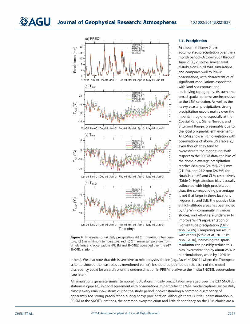
3.1. Precipitation

As shown in Figure 3, theaccumulated precipitation over the 9month period (October 2007 throughJune 2008) displays similar arealdistributions in all WRF simulationsand compares well to PRISMobservations, with characteristics ofsignificant modulations associatedwith land-sea contrast andunderlying topography. As such, thebroad spatial patterns are insensitiveto the LSM selection. As well as theheavy coastal precipitation, strongprecipitation occurs mainly over themountain regions, especially at theCoastal Range, Sierra Nevada, andBitterroot Range, presumably due tothe local orographic enhancement.All LSMs show a high correlation withobservations of above 0.9 (Table 2),even though they tend tooverestimate the magnitude. Withrespect to the PRISM data, the bias ofthe domain average precipitationreaches 88.4 mm (24.7%), 75.5 mm(21.1%), and 95.2 mm (26.6%) forNoah, NoahMP, and CLM, respectively(Table 2). High absolute bias is usuallycollocated with high precipitation;thus, the corresponding percentageis not that large in these locations(Figures 3c and 3d). The positive biasat high-altitude areas has been notedby the WRF community in variousstudies, and efforts are underway toimprove WRF’s representation ofhigh-altitude precipitation [Chinet al., 2009]. Comparing our resultwith others [Subin et al., 2011; Jinet al., 2010], increasing the spatialresolution can possibly reduce thisbias (overestimation by about 25% inour simulations, while by 100% in

others). We also note that this is sensitive to microphysics choice (e.g., Liu et al. [2011] where the Thompsonscheme showed the least bias as mentioned earlier). It should be pointed out that part of the modeldiscrepancy could be an artifact of the underestimation in PRISM relative to the in situ SNOTEL observations(see later).

All simulations generate similar temporal fluctuations in daily precipitation averaged over the 637 SNOTELstations (Figure 4a), in good agreement with observations. In particular, the WRF model captures successfullyalmost every rain/snow storm during the study period, notwithstanding a common discrepancy ofapparently too strong precipitation during heavy precipitation. Although there is little underestimation inPRISM at the SNOTEL stations, the common overprediction and little dependency on the LSM choice are a

Figure 4. Time series of (a) daily precipitation, (b) 2 m maximum tempera-ture, (c) 2 m minimum temperature, and (d) 2 m mean temperature fromsimulations and observations (PRISM and SNOTEL) averaged over the 637SNOTEL stations.

Journal of Geophysical Research: Atmospheres 10.1002/2014JD021827

CHEN ET AL. ©2014. American Geophysical Union. All Rights Reserved. 7277

likely indication that the precipitation discrepancy might result from the deficiency in overlying atmosphericprocesses and/or errors in the reanalysis data used for initial and boundary conditions.

The excessive model precipitation is present and most notable in December–January over all subregions,except Region 6 for the Colorado mountains (Figure 5). Noah gives rise to the largest wet biases over Regions1, 2, and 4, and CLM over Regions 3 and 5. On the whole, the difference among these simulations is small. Thisinsensitivity is consistent with the notion that, as well as the synoptic forcing, terrain forcing is the dominantprocess in determining orographic cloud and precipitation development in the wintertime environment ofthe major precipitation season in the western U.S.

3.2. Temperature

The simulated and observed 2 m maximum temperature (Tmax) are compared in Figures 6 and 4b. All LSMsreplicate the spatial patterns very well, with a pattern correlation coefficient as high as 0.97–0.98.Additionally, the daily evolution pattern is captured reasonably as well. An evident deficiency is thewidespread cold biases and most striking over high-elevated mountain peaks and ridges, with an areal and

Figure 5. Daily mean precipitation difference for each month between simulations and observations averaged over the SNOTEL stations for (a) whole domain and(b–g) subdomains.

Journal of Geophysical Research: Atmospheres 10.1002/2014JD021827

CHEN ET AL. ©2014. American Geophysical Union. All Rights Reserved. 7278

temporal mean of �2.2°C, �1.2°C, and�0.4°C for Noah, NoahMP, and CLM, respectively (Table 2). It is readilyseen that CLM and Noah are, respectively, the best and the worst performer.

Like the maximum temperature, the WRF model reproduces the broad spatial variations (Figure 7) andseasonal changes (Figure 4c) for 2 m minimum temperature (Tmin). The pattern correlation ranges from0.87–0.94, slightly less than the maximum temperature counterpart. Distinct to the prevalent cold bias inTmax, a warm bias in Tmin is dominant over the entire domain with an average value of 0.6°C, 1.4°C, and 1.1°Cfor Noah, NoahMP, and CLM, respectively (Table 2). But Tmin is underestimated by asmuch as 2–7°C over somesnow-covered mountains. With respect to the SNOTEL stations, a cold bias is seen with an average value of�4.0°C,�1.7°C, and�4.1°C for Noah, NoahMP, and CLM, respectively (Table 3). Overall, NoahMP is superior toNoah and CLM as far as Tmin is concerned, which may be related to the lower latent heat flux in NoahMP(see Figure 16g later). More energy is trapped in the surface layer to keep the Tmin warmer than other LSMs,especially Noah.

Of note is the salient differences in both Tmax and Tmin during the snowpack melting season, particularly overthe period when Tmax is near 0°C (Figure 4b). This phenomenon may be attributed to the different treatment

(a) OBS (oC)

(b) MODEL (oC)

NOAH NOAHMP CLM

(c) BIAS (oC)

Figure 6. Spatial distribution of observed and simulated 2 m maximum temperature averaged over October 2007 through June 2008. (a) PRISM, (b) model results,and (c) bias (model-observation).

Journal of Geophysical Research: Atmospheres 10.1002/2014JD021827

CHEN ET AL. ©2014. American Geophysical Union. All Rights Reserved. 7279

of snow physics, especially melting processes, in the LSMs. On the whole, the surface temperature simulationis more sensitive to the land surface parameterizations than precipitation in the present case.

No matter which LSM is used, all subregions feature a persistent cold bias throughout the integration overthe mountains (Figures 8 and 9). It is obvious that CLM and NoahMP better Noah in Tmax forecasting, andNoahMP outperforms Noah and CLM in Tmin over high-elevation subdomains. However, Noah performs best toreproduce 2 m diurnal temperature range with a mean discrepancy of�0.8°C, while NoahMP underestimates itand CLM overestimates it with an average value of�1.2°C and 1.6°C, respectively (Table 3). The composite dailytemperature in Figure 10 also reveals a largest diurnal cycle in CLM and a smallest one in NoahMP.

3.3. Snow Water Equivalent

Figure 11 presents a comparison of the modeled SWE peak values with the SNOTEL data. The geographicaldistributions are strongly modulated by the mesoscale terrain and show a good correspondence with theprecipitation (Figure 3) and temperature (Figures 6 and 7). An understandable characteristic is the collocationof high SWE and precipitation amount usually at high elevations and cold temperatures. In spite of the

(a) OBS(oC)

(b) MODEL (oC)

NOAH NOAHMP CLM

(c) BIAS (oC)

Figure 7. Same as Figure 6 but for 2 m minimum temperature.

Journal of Geophysical Research: Atmospheres 10.1002/2014JD021827

CHEN ET AL. ©2014. American Geophysical Union. All Rights Reserved. 7280

encouraging agreement with observations, however, the model overestimates the SWE in the Coastal Rangeand some ridges of other mountain ranges and underestimates the amount in the Colorado Rockies andlow elevations (valleys), in good correspondence with the respective positive and negative precipitationbiases (Figure 3). The average SWE peak value over the 637 SNOTEL stations is 474.7 mm, 540.6 mm, and604.7 mm for the Noah, NoahMP, and CLM, respectively, all being below the observed 638.7 mm. Overall,CLM is more consistent with observations than Noah and NoahMP (This can be also seen from Figure 2, inwhich CLM has the smallest standardized bias with a similar correlation coefficient to Noah and NoahMP).The superiority of CLM is further confirmed in the scatterplot of simulated SWE peaks versus observations(Figure 12); Noah and NoahMP underestimate the SWE peak at a great majority of stations, and CLM ismuch closer to the reality.

Figure 13 compares the simulated and observed SWE peak time. The three LSMs generate a comparabletiming at most locations, characteristic of a late February to early March timing in the southern part of thedomain and also northern low elevations and an April–May timing in northern high elevations. As comparedto observations, the modeled SWE peaks too early in the southern and low-elevation areas but too late in thenorthern and high mountain areas, closely related to the temperature, especially Tmin, biases (Figure 7). Morethan 97% of the stations with a late SWE peak also underestimate Tmin to varying degrees. The timing biasranges from �54 to 1, �38 to 3, and �28 to 28 days, with a mean discrepancy of �23.0, �11.8, and 1.6 daysfor Noah, NoahMP, and CLM, respectively. As for the above-presented SWE peak amount, CLM outperformsNoah and NoahMP, and NoahMP performs better than Noah in the timing. Therefore, it is tentativelyconcluded that NoahMP has a better performance than Noah on the SWE simulation, and CLM is the best, asfound in the Taylor diagram (Figure 2). These results may suggest that a more detailed description of landsurface processes in NoahMP and CLM play a positive role in the model performance.

Figure 14 shows the daily evolution and monthly averages at the SNOTEL sites. The modeled SWE, albeitsomewhat underestimated, closely follows the observations in the early accumulation period (e.g., Octoberthrough December). Thereafter, the performance diverges between the three LSMs. Noah displays a flat peakand biases low from mid-January through mid-April, indicative of unrealistically strong melting completelyoffsetting snowfall contributions. This snowpack representation deficiency in Noah has been reported insome previous studies [e.g., Livneh et al., 2009; Rasmussen et al., 2011]. In contrast, snowpack in CLM andNoahMP exhibits a persistent expansion until the middle of April and a subsequent steady ablation, inresemblance with the observations. On the whole, CLM matches the observation best, with an exception ofthe too slowmelting due to cold temperature biases in late spring and early summer, whereas both Noah andNoahMP tend to underpredict the snowpack magnitude throughout the integration.

Table 3. Statistics of Time Average Variables From WRF Simulations and SNOTEL Data

Variables Units Noah NoahMP CLM SNOTEL

Snow water equivalent mm 190.2 234.7 284.0 278.4Precipitation mm d�1 3.8 3.6 3.8 3.4Snowfall from diagnosis mm d�1 3.0 2.9 3.2 -Snowfall from microphysics mm d�1 3.0 2.8 3.0 -2 m maximum temperature °C 1.1 3.0 3.4 5.92 m minimum temperature °C �9.0 �6.7 �9.1 �5.02 m diurnal temperature range °C 10.1 9.7 12.5 10.92 m mean temperature °C �3.9 �1.9 �2.8 0.1Surface albedo % 47.1 31.3 30.2 -Downward shortwave flux W/m2 197.5 195.5 193.5 -Upward shortwave flux W/m2 87.9 58.2 55.2 -Net shortwave flux W/m2 109.6 137.3 138.3 -Downward longwave flux W/m2 235.6 233.9 236.1 -Upward longwave flux W/m2 285.4 305.3 304.8 -Net longwave flux W/m2 �49.9 �71.4 �68.8 -Net radiation W/m2 59.7 66.0 69.6 -Latent heat flux W/m2 42.6 21.0 25.7 -Sensible heat flux W/m2 �2.3 34.6 34.8 -Ground heat flux W/m2 1.8 9.3 8.7 -Surface temperature °C �3.7 �2.6 �1.6 -

Journal of Geophysical Research: Atmospheres 10.1002/2014JD021827

CHEN ET AL. ©2014. American Geophysical Union. All Rights Reserved. 7281

The performance shows some geographical dependence (Figure 15). For instance, CLM (NoahMP) performsbetter in Regions 1 and 2 (Regions 3 and 4) than in other regions. An intercomparison at all mountainranges indicates the superiority of CLM in snowpack buildup, peak timing, and value and also a constantunderprediction in Noah and NoahMP. Considering the accurate or even somewhat overestimate ofprecipitation in all simulations, the apparent SWE underprediction implies snow physics deficiencies inNoah and NoahMP.

4. Discussion

The preceding evaluation indicates a good agreement of the modeled precipitation with observation,irrespective of the LSM selection. This result is presumably attributable to an adequate representation of thecomplex topography and explicit cloud-precipitation physics in the high-resolution convection-allowingWRFmodel, as well as the realistic large-scale forcing provided by the CFSR data, consistent with previousmodeling studies of cold season precipitation over the Colorado Rockies [e.g., Ikeda et al., 2010; Rasmussenet al., 2011]. The insensitivity to LSMs possibly results from the relatively weak land surface energy andmoisture exchange during the cold season, which covers most of the present experimental period, as

Figure 8. Same as Figure 5 but for 2 m maximum temperature.

Journal of Geophysical Research: Atmospheres 10.1002/2014JD021827

CHEN ET AL. ©2014. American Geophysical Union. All Rights Reserved. 7282

demonstrated in Liu et al. [2011]. An evident advantage of the weak LSM dependency of model precipitationis its facilitation for interpreting snowpack differences among the tested LSMs.

All models overestimate the precipitation and underestimate the SWE with respect to SNOTEL observations.The excessive precipitation could be attributed to the choice of other physics parameterizations, modelresolution, and large-scale forcing, which is mentioned in Chin et al. [2009] and Liu et al. [2011]. The snowpackrepresentation deficiency in Noah has been reported in some previous studies [e.g., Livneh et al., 2009;Rasmussen et al., 2011], and may be partially attributable to the lack of a canopy treatment or multilevel snow[Barlage et al., 2010]. However, the inconsistency between precipitation overestimation and SWEunderestimation even in cold seasons shows that the precipitation may not be so bad. The instrumentalerrors in snowfall measurements may also lead to underestimation of the observation, despite the fact thatthe under catch is not so large (approximately 10–15%).

In spite of the comparable precipitation, salient differences and thus a great sensitivity are found in snowpacksimulations. Furthermore, all experiments have negative SWE biases except for the melting season in CLM,notwithstanding an over 10% precipitation overprediction, suggesting an existence of snow physicsdeficiencies in these LSMs. Although a clear explanation is rather difficult, our diagnosis illustrates that the

Figure 9. Same as Figure 5 but for 2 m minimum temperature.

Journal of Geophysical Research: Atmospheres 10.1002/2014JD021827

CHEN ET AL. ©2014. American Geophysical Union. All Rights Reserved. 7283

diversity in partitioning precipitation into rainfall and snowfall is an important factor accounting for asignificant portion of the SWE difference among the LSMs. In general, the partition methods for the threeland surface schemes are as follows:

SNOAH ¼ P; Ta ≤ T frz; or; Ts ≤ T frz0; otherwise

�; (1)

SNOAHMP ¼

P; Ta ≤ T frz þ 0:5

P� 1� �54:632þ 0:2� Tað Þ½ �; T frz þ 0:5 < Ta ≤ T frz þ 2:0

P� 0:6; T frz þ 2:0 < Ta ≤ T frz þ 2:5

0; Ta > T frz þ 2:5

8>>><>>>:

; (2)

SCLM ¼ P; Ta ≤ T frz þ 2:5

0; Ta > T frz þ 2:5

�; (3)

Figure 10. Simulated diurnal cycles of temperature averaged over SNOTEL stations for (a) whole domain and (b–g) subdomains.

Journal of Geophysical Research: Atmospheres 10.1002/2014JD021827

CHEN ET AL. ©2014. American Geophysical Union. All Rights Reserved. 7284

where SNOAH, SNOAHMP, and SCLM are snowfall in Noah, NoahMP, and CLM, respectively, P precipitation, Ta theair temperature of bottom model layer, and Tfrz freezing temperature, equal to 273.16 K. Apparently, thesehypotheses would lead to most snowfall in CLM, followed by NoahMP, and least in Noah, for the sametemperature and precipitation. It is worth noting that an alternative partition method in Noah is based on themicrophysics-derived ratio of snow to precipitation for some configurations (e.g., Thompson microphysics inour simulation). Table 3 shows the simulated precipitation and snow amount averaged over the SNOTELstations. Approximately 78.2%, 81.0%, and 84.7% of surface precipitation is categorized into snowfall in Noah,NoahMP, and CLM, respectively, and qualitatively, this is consistent with the SWE differentiation, namely,the least SWE in Noah and the largest SWE in CLM. Assuming that the additional snowfall in CLM does notmelt and sublimate at all, the cumulative effect would account for 82% of the temporal average SWEdifference from NoahMP and 37% of the difference from Noah (The difference in cumulative snowfallbetween CLM and Noah is 34.99 mm, while that between CLM and NoahMP is 40.45 mm. The temporalaverage SWE differences are 93.8 mm and 49.3 mm.). Also, note that the different snowfall-rainfall ratioscannot be explained in terms of the mean temperature differences; for instance, Noah produced thecoldest temperature but the smallest snowfall fraction.

The foregoing analysis illustrates that the temperature-based snow-rain distinction could induce aconsiderable uncertainty for SWE estimation. Nevertheless, this undesirable subjective partitioning isunavoidable in coarse-resolution numerical models, because conventional convective parameterizationsdo not provide the precipitation type information. However, in fine-resolution convection-permitting

Figure 11. Observed and simulated SWE peak values. (a) SNOTEL, (b) model results, (c) bias (model-observation), and (d) percentage bias.

Journal of Geophysical Research: Atmospheres 10.1002/2014JD021827

CHEN ET AL. ©2014. American Geophysical Union. All Rights Reserved. 7285

simulations without using a convection scheme, such as the ones in this study, model precipitationis determined solely by the cloud-precipitation microphysics which explicitly provides precipitationcategories. For instance, the Thompson microphysics scheme used here contains three types ofprecipitation, namely, rain, snow, and graupel. Accordingly, an appealing improvement forapplications to high-resolution models is the utilization of microphysics-generated precipitationtypes, replacing the subjective temperature-dependent snowfall-rainfall diagnosis in existing LSMs.This type of microphysics-based approach is being implemented into NoahMP (M. Barlage,personal communication, 2014).

In addition to the contrasting snow-rain separation, a comparison of land surface variables in Figure 16evinces other contributing factors behind the different surface temperature and snowpack among theseLSMs. The albedo in Noah is much higher than in NoahMP and CLM, particularly during November–March(Figure 16c). A high albedo leads to a high reflection of short wave radiation (Figure 16d), accounting for theaforementioned largest cold bias in the simulation with Noah. The low surface temperature, in turn,limits sensible heat transport (Figure 16h) and longwave radiative cooling (Figure 16e). As such, moreenergy could be stored for snow melting, causing a low snowpack (Figure 16a), a wet land surfaceand latent heat transport enhancement (Figure 16g). These differences are highly related to thedifferences in snow physics in LSMs. For example, combined surface layer of vegetation and snow inNoah would tend to underestimate the ground heat flux because of the combined thickness ofsnowpack and half of the top layer soil, which leaves too much energy at the snow surface and thusprone to snowmelt (also can be found in Figure 16i). Additionally, the combined layer cannot wellrepresent the percolation, retention, and refreezing of melt liquid water; shallow soil column is notable to capture the critical zone (down to 5 m) to which the surface energy budgets are most

Figure 12. The scatter plot of simulated versus observed SWE peak value for (a) Noah, (b) NoahMP, and (c) CLM.

Journal of Geophysical Research: Atmospheres 10.1002/2014JD021827

CHEN ET AL. ©2014. American Geophysical Union. All Rights Reserved. 7286

sensitive; frozen soil is too impervious which leads to too much surface runoff and less infiltrationin spring or early summer [Niu et al., 2011]. Some of these problems are improved in NoahMP andCLM and thus better model performances are found. These differences in snow physics in LSMs maycontribute to the difference in SWE, although it is difficult to know how important they are.

Figure 13. Same as Figure 11 but for SWE peak time (day).

(a)

(b)

Figure 14. (a) Daily and (b) monthly SWE difference between simulations and observations averaged at 637SNOTEL stations.

Journal of Geophysical Research: Atmospheres 10.1002/2014JD021827

CHEN ET AL. ©2014. American Geophysical Union. All Rights Reserved. 7287

Vegetation plays an important role on snow process [Jin and Wen, 2012]. The performance of each LSM relieson the underlying land use. As shown in Figure 17, for example, CLM reproduces the SWE reasonably wellover the crop- and grass-covered areas but has a remarkable low bias over the deciduous forests and amoderate high bias during the melting season over the evergreen forests. This regional contrast may suggestdeficient treatment of physical processes inside tree canopies. In addition, although the current version,CLM4, contains some significant improvements in surface input data [Lawrence and Chase, 2007], thecoupling of vegetation type between WRF and CLM is based on a lookup table, and there is room for furtherimprovement in this aspect.

5. Conclusions

This study evaluated and compared the performance of three land surface schemes coupled with the WRFmodel in precipitation, temperature, and snowpack simulations over the western U.S. The 9 monthexperimental period from October 2007 to June 2008 enabled an investigation of the LSM’s capability indepicting both snowpack buildup and ablation. The results would be useful for guiding future developmentsand improvements of these tested LSMs. Our primary findings are summarized as follows.

Figure 15. Same as Figure 5 but for SWE (mm).

Journal of Geophysical Research: Atmospheres 10.1002/2014JD021827

CHEN ET AL. ©2014. American Geophysical Union. All Rights Reserved. 7288

1. Regardless of the selected LSM, major observed spatiotemporal characteristics were captured reasonablywell, presumably attributable to the adequate representation of the underlying mesoscale terrain andexplicit representation of precipitating convection.

2. All LSMs generated a cold temperature bias (both maximum and minimum) over the snow-topped moun-tain ridges. By and large, CLM was superior for maximum temperatures, whereas NoahMP performed bestfor minimum temperatures. The coldest bias in Noahwas found in association with the large surface albedo.

3. CLM was most skillful in depicting snowfall accumulation and SWE peaks, despite a too slow ablation par-ticularly in the needleleaf covered areas. Noah significantly underpredicted SWE amount in both theaccumulating and melting seasons.

Figure 16. Time series of daily land surface variables simulated by the three LSMs. (a) snow water equivalent, (b) snowfall, (c) surface albedo, (d) net-absorbed short-wave flux, (e) net-absorbed longwave flux, (f ) net radiative flux, (g) surface latent heat flux, (h) surface sensible heat flux, (i) ground flux, and (j) surface temperature.

Journal of Geophysical Research: Atmospheres 10.1002/2014JD021827

CHEN ET AL. ©2014. American Geophysical Union. All Rights Reserved. 7289

4. An appreciable part of the SWE differences between the three LSMs resulted from the subjective snowfall-rainfall partitioning. Accordingly, we strongly suggest the use of a microphysics-based approach for theidentification of precipitation types in high-resolution convection-permitting models.

ReferencesBarlage, M., F. Chen, M. Tewari, K. Ikeda, D. Gochis, J. Dudhia, R. Rasmussen, B. Livneh, M. Ek, and K. Mitchell (2010), Noah land surface model

modifications to improve snowpack prediction in the Colorado Rocky Mountains, J. Geophys. Res., 115, D22101, doi:10.1029/2009JD013470.Bowling, L. C., et al. (2003), Simulation of high-latitude hydrological processes in the Torne-Kalix basin-PILPS Phase 2 (e). 1: Experiment

description and summary intercomparisons, Global Planet. Change, 38, 1–30, doi:10.1016/S0921-8181(03)00003-1.Cess, R. D., et al. (1991), Interpretation of snow-climate feedback as produced by 17 general circulation models, Science, 253, 888–892.Chen, F., and J. Dudhia (2001), Coupling an advanced land surface hydrology model with the Penn State-NCARMM5modeling system. Part I.

Model implementation and sensitivity, Mon. Weather Rev., 129, 569–585.Chin, H.-N. S., P. M. Caldwell, and D. C. Bader (2009), Exploration of California wintertime model wet bias: Sensitivity of WRF physics and

measurement uncertainty, WRF Users Workshop, 5B.7, NCAR, Boulder, Colo. [Available at http://www.mmm.ucar.edu/wrf/users/workshops/WS2009/abstracts/5B-07.pdf.]

Cohen, J., and D. Entekhabi (2001), The influence of snow cover on Northern Hemisphere climate variability, Atmos. Ocean, 39(1), 35–53.Collins, M., et al. (2013), Long-term climate change: Projections, commitments and irreversibility, in Climate Change 2013: The Physical

Science Basis. Contribution of Working Group I to the Fifth Assessment Report of the Intergovernmental Panel on Climate Change, edited byT. F. Stocker et al., pp. 1029–1136, Cambridge Univ. Press, Cambridge, U. K., and New York.

Daly, C., M. Halbleib, J. I. Smith, W. P. Gibson, M. K. Doggett, G. H. Taylor, J. Curtis, and P. P. Pasteris (2008), Physiographically sensitive mapping ofclimatological temperature and precipitation across the conterminous United States, Int. J. Climatol., 28, 2031–2064, doi:10.1002/joc.1688.

Ek, M. B., K. E. Mitchell, Y. Lin, E. Rogers, P. Grunmann, V. Koren, G. Gayno, and J. D. Tarpley (2003), Implementation of Noah land surfacemodeladvancements in the National Centers for Environmental Prediction operational mesoscale Eta model, J. Geophys. Res., 108(D22), 8851,doi:10.1029/2002JD003296.

Flanner, M. G., and C. S. Zender (2006), Linking snowpack microphysics and albedo evolution, J. Geophys. Res., 111, D12208, doi:10.1029/2005JD006834.

Grant, L. O., and A. M. Kahan (1974), Weather modification for augmenting orographic precipitation, in Weather and Climate Modification,edited by W. N. Hess, pp. 282–317, John Wiley, New York.

Groisman, P. Y., T. R. Karl, R. W. Knight, and G. L. Stenchikov (1994), Changes of snow cover, temperature, and radiative heat balance over theNorthern Hemisphere, J. Clim., 7, 1633–1656.

Hoerling, M., and J. Eischeid (2006), Past peak water in the Southwest, Southwest Hydrol., 35, 18–19.Hong, S. Y., andH. L. Pan (1996), Nonlocal boundary layer vertical diffusion in amedium-range forecastmodel,Mon.Weather Rev., 124(10), 2322–2339.Iacono, M. J., J. S. Delamere, E. J. Mlawer, M. W. Shephard, S. A. Clough, and W. D. Collins (2008), Radiative forcing by long-lived greenhouse

gases: Calculations with the AER radiative transfer models, J. Geophys. Res., 113, D13103, doi:10.1029/2008JD009944.Ikeda, K., et al. (2010), Simulation of seasonal snowfall over Colorado, Atmos. Res., 97, 462–477, doi:10.1016/j.atmosres.2010.04.010.Intergovernmental Panel on Climate Change (2007), Contribution of working group I to the fourth assessment report of the IPCC. [Available

at http://ipcc-wg1.ucar.edu/index.html.]Jimenez, P. A., J. J. Dudhia, F. Gonzalez-Rouco, J. Navarro, J. P. Montavez, and E. Garcia-Bustamante (2012), A revised scheme for the WRF

surface layer formulation, Mon. Weather Rev., 140, 898–918.Jin, J., and N. L. Miller (2007), Analysis of the impact of snow on daily weather variability in mountainous regions using MM5, J. Hydrometeorol., 8,

245–258, doi:10.1175/JHM565.1.

Figure 17. Time series of simulated and observed daily SWE for different types of vegetation.

AcknowledgmentsThe authors thank Jiming Jin of UtahState University and Fei Chen of NCAR/RAL for their helpful comments andsuggestions. This study was supportedby the National Natural ScienceFoundation of China (grant 41105062),the National Public Sector(Meteorological) Special Research(grant GYHY201206006). The CFSR dataare available at NCAR’s CISL ResearchData Archive (http://rda.ucar.edu/data-sets/ds093.0/), the PRISM data can befound at PRISM Climate Group ofNorthwest Alliance for ComputationalScience and Engineering, Oregon StateUniversity (http://www.prism.oregon-state.edu), and the SNOTEL data areobtained at the Natural ResourcesConservation Service (http://www.wcc.nrcs.usda.gov/ftpref/data/).

Journal of Geophysical Research: Atmospheres 10.1002/2014JD021827

CHEN ET AL. ©2014. American Geophysical Union. All Rights Reserved. 7290

Jin, J., and L. Wen (2012), Evaluation of snowmelt simulation in the Weather Research and Forecasting model, J. Geophys. Res., 117, D10110,doi:10.1029/2011JD016980.

Jin, J., N. L. Miller, and N. Schegel (2010), Sensitivity study of four land surface schemes in the WRF model, Adv. Meteorol., 2010, 167,436,doi:10.1155/2010/167436.

Koren, V., J. C. Schaake, K. E. Mitchell, Q. Y. Duan, F. Chen, and J. M. Baker (1999), A parameterization of snowpack and frozen ground intendedfor NCEP weather and climate models, J. Geophys. Res., 104, 19,569–19,585, doi:10.1029/1999JD900232.

Lawrence, D. M., et al. (2011), Parameterization improvements and functional and structural advances in version 4 of the Community LandModel, J. Adv. Model. Earth Syst., 3, M03001, doi:10.1029/2011MS000045.

Lawrence, P. J., and T. N. Chase (2007), Representing a new MODIS consistent land surface in the Community Land Model (CLM 3.0),J. Geophys. Res., 112, G01023, doi:10.1029/2006JG000168.

Leung, L. R., and Y. Qian (2003), The sensitivity of precipitation and snowpack simulations to model resolution via nesting in regions ofcomplex terrain, J. Hydrometeorol., 4, 1025–1043, doi:10.1175/1525-7541(2003)004<1025:TSOPAS>2.0.CO;2.

Leung, L. R., Y. Qian, J. Han, and J. Roads (2003), Intercomparison of global reanalyses and regional simulations of cold season water budgetsin the western United States, J. Hydrometeorol., 4, 1067–1087.

Liston, G. E. (2004), Representing subgrid snow cover heterogeneities in regional and global models, J. Clim., 17, 1381–1397.Liu, C. H., K. Ikeda, G. Thompson, R. Rasmussen, and J. Dudhia (2011), High-resolution simulations of wintertime precipitation in the Colorado

headwaters region: Sensitivity to physics parameterizations, Mon. Weather Rev., 139, 3533–3553.Livneh, B., Y. Xia, K. Mitchell, M. Ek, and D. P. Lettenmaier (2009), Noah LSM snowmodel diagnostics and enhancements, J. Hydrometeorol., 11,

721–738.Livneh, B., Y. Xia, K. E. Mitchell, M. B. Ek, and D. P. Lettenmaier (2010), Noah LSM snow model diagnostics and enhancements, J. Hydrometeorol., 11,

721–738, doi:10.1175/2009JHM1174.1.Lu, Y., and L. M. Kueppers (2012), Surface energy partitioning over four dominant vegetation types across the United States in a coupled

regional climate model (Weather Research and Forecasting Model 3-Community Land Model 3.5), J. Geophys. Res., 117, D06111,doi:10.1029/2011JD016991.

McCabe, G. J., and P. M. Clark (2005), Trend and variability in snowmelt runoff in the western United States, J. Hydrometeorol., 6(4), 476–482,doi:10.1175/JHM428.1.

Niu, G. Y., et al. (2011), The community Noah land surface model with multiparameterization options (Noah-MP): 1. Model description andevaluation with local-scale measurements, J. Geophys. Res., 116, D12109, doi:10.1029/2010JD015139.

Oleson, K. W., et al. (2010), Technical description of version 4.0 of the Community Land Model (CLM), Tech. Note NCAR/TN-478+STR, 257 pp.,Natl. Cent. for Atmos. Res., Boulder, Colo.

Rasmussen, R. M., et al. (2001), Weather Support to Deicing Decision Making (WSDDM): A winter weather nowcasting system, Bull. Am.Meteorol. Soc., 82, 579–595.

Rasmussen, R. M., et al. (2011), High-resolution coupled climate runoff simulations of seasonal snowfall over Colorado: A process study ofcurrent and warmer climate, J. Clim., 24, 3015–3048, doi:10.1175/2010JCLI3985.1.

Rauscher, S. A., J. S. Pal, N. S. Diffenbaugh, and M. M. Benedetti (2008), Future changes in snowmelt-driven runoff timing over the western US,Geophys. Res. Lett., 35, L16703, doi:10.1029/2008GL034424.

Saha, S., et al. (2010), The NCEP climate forecast system reanalysis, Bull. Am. Meteorol. Soc., 91, 1015–1057.Seager, R., et al. (2007), Model projections of an imminent transition to a more arid climate in southwestern North America, Science, 316,

1181–1184.Serreze, M. C., M. P. Clark, R. L. Amstrong, D. A. McGinnis, and R. S. Pulwarty (1999), Characteristics of western United States snowpack from

snowpack telemetry (SNOTEL) data, Water Resour. Res., 35, 2145–2160, doi:10.1029/1999WR900090.Serreze, M. C., M. P. Clark, and A. Frei (2001), Characteristics of large snowfall events in themontane western United States as examined using

snowpack telemetry (SNOTEL) data, Water Resour. Res., 37, 675–688, doi:10.1029/2000WR900307.Skamarock, W. C., J. B. Klemp, J. Dudhia, D. O. Gill, D. M. Barker, M. G. Duda, X.-Y. Huang, W. Wang, and J. G. Powers (2008), A description of

advanced research WRF version 3, Tech. Note NCAR/TN-475+STR, 113 pp., Natl. Cent. for Atmos. Res., Boulder, Colo.Slater, A. G., T. J. Bohn, J. L. McCreight, M. C. Serreze, and D. P. Lettenmaier (2007), A multimodel simulation of pan-Arctic hydrology,

J. Geophys. Res., 112, G04S45, doi:10.1029/2006JG000303.Subin, Z. M., W. J. Riley, J. Jin, D. S. Christianson, M. S. Torn, and L. M. Kueppers (2011), Ecosystem feedbacks to climate change in California:

Development, testing, and analysis using a coupled regional atmosphere and land surface model (WRF3-CLM3.5), Earth Interact., 15, 1–38,doi:10.1175/2010EI331.1.

Sun, S., J. Jin, and Y. Xue (1999), A simple snow-atmosphere-soil transfer model, J. Geophys. Res., 104, 19,587–19,597, doi:10.1029/1999JD900305.Taylor, K. E. (2001), Summarizing multiple aspects of model performance in a single diagram, J. Geophys. Res., 106, 7183–7192, doi:10.1029/

2000JD900719.Thompson, G., P. R. Field, R. M. Rasmussen, and W. D. Hall (2008), Explicit forecasts of winter precipitation using an improved bulk micro-

physics scheme. Part II: Implementation of a New snow parameterization, Mon. Weather Rev., 136, 5095–5115.Tian, X., A. Dai, D. Yang, and Z. Xie (2007), Effects of precipitation-bias corrections on surface hydrology over northern latitudes, J. Geophys.

Res., 112, D14101, doi:10.1029/2007JD008420.Wang, A. H., and X. B. Zeng (2009), Improving the treatment of the vertical snow burial fraction over short vegetation in the NCAR CLM3, Adv.

Atmos. Sci., 26(5), 877–886, doi:10.1007/s00376-009-8098-3.Wang, Z., X. Zeng, and M. Decker (2010), Improving snow processes in the Noah land model, J. Geophys. Res., 115, D20108, doi:10.1029/

2009JD013761.Yang, D., B. E. Goodison, J. R. Metcalfe, V. S. Golubev, R. Bates, T. Pangburn, and C. L. Hanson (1998), Accuracy of NWS 8″ standard nonrecording

precipitation gauge: Results and application of WMO intercomparison, J. Atmos. Oceanic Technol., 15, 54–68.Yang, Z. L., et al. (2011), The community Noah land surface model with multiparameterization options (Noah–MP): 2. Evaluation over global

river basins, J. Geophys. Res., 116, D12110, doi:10.1029/2010JD015140.

Journal of Geophysical Research: Atmospheres 10.1002/2014JD021827

CHEN ET AL. ©2014. American Geophysical Union. All Rights Reserved. 7291