Very high resolution regional climate model simulations over Greenland: Identifying added value

Very high resolution regional climate model simulationsover Greenland: Identifying added value

Philippe Lucas-Picher,1,2 Maria Wulff-Nielsen,3,4 Jens H. Christensen,3

Guðfinna Aðalgeirsdóttir,3 Ruth Mottram,3 and Sebastian B. Simonsen3,5

Received 18 May 2011; revised 18 November 2011; accepted 18 November 2011; published 25 January 2012.

[1] This study presents two simulations of the climate over Greenland with the regionalclimate model (RCM) HIRHAM5 at 0.05° and 0.25° resolution driven at the lateralboundaries by the ERA-Interim reanalysis for the period 1989–2009. These simulations arevalidated against observations from meteorological stations (Danish MeteorologicalInstitute) at the coast and automatic weather stations on the ice sheet (Greenland ClimateNetwork). Generally, the temperature and precipitation biases are small, indicating arealistic simulation of the climate over Greenland that is suitable to drive ice sheet models.However, the bias between the simulations and the few available observations does notreduce with higher resolution. This is partly explained by the lack of observations inregions where the higher resolution is expected to improve the simulated climate.The RCM simulations show that the temperature has increased the most in the northern partof Greenland and at lower elevations over the period 1989–2009. Higher resolutionincreases the relief variability in the model topography and causes the simulatedprecipitation to be larger on the coast and smaller over the main ice sheet compared to thelower-resolution simulation. The higher-resolution simulation likely represents theGreenlandic climate better, but the lack of observations makes it difficult to validate fully.The detailed temperature and precipitation fields that are generated with the higherresolution are recommended for producing adequate forcing fields for ice sheet models,particularly for their improved simulation of the processes occurring at the steep marginsof the ice sheet.

Citation: Lucas-Picher, P., M. Wulff-Nielsen, J. H. Christensen, G. Aðalgeirsdóttir, R. Mottram, and S. B. Simonsen (2012),Very high resolution regional climate model simulations over Greenland: Identifying added value, J. Geophys. Res., 117, D02108,doi:10.1029/2011JD016267.

1. Introduction

[2] Remote sensing observations show that the Greenlandice sheet is thinning and losing mass at an accelerating rate inthe recent years [Luthcke et al., 2006; Pritchard et al., 2009;Velicogna, 2009]. In the literature, considerable discrepanciesappear between the mass balance estimates of the Greenlandice sheet and their inherited uncertainties [Dahl-Jensen et al.,2009, Table 2.3]. Even different estimates applying similarmethodology and data sets show discrepancies [Sørensenet al., 2011; Zwally et al., 2011], which may be partlyexplained by the limited knowledge of the Greenland climate.

Without robust and validated climate forcing, it is not possibleto compute realistic estimates of the surface mass balance andsurface evolution of the Greenland ice sheet.[3] Coastal weather stations have been operated in Green-

land by the Danish Meteorological Institute (DMI) since thelate 19th century [Cappelen, 2010]. However, the Greenlandice sheet itself suffers from both poor spatial and temporalcoverage of observations. Although, this situation hasrecently improved considerably with an increasing number ofweather stations on the ice sheet, from the GC-Net stations[Steffen and Box, 2001], the K transect [van de Wal et al.,2005] and the monitoring project PROMICE [Ahlstrømet al., 2008]. (GC-Net data are available online at http://cires.colorado.edu/science/groups/steffen/gcnet/.) There arestill large regions without any weather data, especially in theablation zone where the Greenland ice sheet loses most mass.[4] Climate models are thus the only physically sound

tools that are capable of filling the spatial gap between theweather stations and to enable computation of the past andfuture evolution of the climate over Greenland. Global cli-mate models (GCMs), with horizontal resolution of about100–200 km [Randall et al., 2007], are too coarse to repre-sent the detailed topography that controls the surface

1Centre National de Recherches Météorologiques, Météo-France,Toulouse, France.

2Also at Danish Climate Centre, Danish Meteorological Institute,Copenhagen, Denmark.

3Danish Meteorological Institute, Copenhagen, Denmark.4Also at Planetary Physics and Geophysics, Niels Bohr Institute,

University of Copenhagen, Copenhagen, Denmark.5Also at Centre for Ice and Climate, Niels Bohr Institute, University of

Copenhagen, Copenhagen, Denmark.

Copyright 2012 by the American Geophysical Union.0148-0227/12/2011JD016267

JOURNAL OF GEOPHYSICAL RESEARCH, VOL. 117, D02108, doi:10.1029/2011JD016267, 2012

D02108 1 of 16

http://dx.doi.org/10.1029/2011JD016267

forcing, such as the steep slopes of the ice sheet and thedescription of the fjords necessary to simulate the mesoscaleclimate in the coastal regions. For the last 20 years (see thereview in the work of Giorgi [2006]), regional climatemodels (RCMs) have been used to efficiently increase theresolution of climate simulations to the scale of a few tens ofkilometers. At this higher resolution, the RCMs describebetter the steep topography in the ablation zone and theeffects of orographically enhanced precipitation generatedon the upstream slopes of the mountains, with less precipi-tation on the lee side [e.g., Dahl-Jensen et al., 2009]. Theimproved description of these effects is important to accu-rately compute the accumulation and the surface mass bal-ance, especially when the climate model is coupled with, orotherwise used to drive, an ice sheet model. The RCMemploys a limited area domain that is driven at the bound-aries by large-scale atmospheric fields from a GCM or byreanalysis data. RCMs can therefore be considered as smartphysically consistent interpolators because they are dynam-ically downscaling the large-scale atmospheric fields pro-vided at their boundaries.[5] A number of RCMs have been used to simulate the

recent past climate over Greenland. In their validation of theclimate simulated with the HIRHAM4 RCM, Box and Rinke[2003] recognized the importance of using an accuratedescription of the topography of the Greenland ice sheet inorder to reduce the biases in the climate simulation. Fettweis[2007] computed the surface mass balance of the Greenlandice sheet by using the regional climate model MAR for theperiod 1979–2006, but without validating the RCM climateoutput against observations. Later, Ettema et al. [2009]computed higher surface mass balance than MAR over theice sheet with RACMO2 during the period 1958–2007.According to Ettema et al. [2009], the higher surface massbalance with RACMO2 is likely to be resulting from thehigher precipitation and melt computed with a higher spatialresolution of 11 km compared to the 25 km resolution thatMAR used. The higher resolution facilitates capturing snowaccumulation peaks that coarser RCMs miss because ofpoorer representation of the topography [Ettema et al.,2009].[6] In another study, Ettema et al. [2010] demonstrated

that RACMO2 can simulate the present-day near-surfacecharacteristics of Greenland by doing a systematic compar-ison of the model output against observations from coastaland ice sheet weather stations. Burgess et al. [2010] used theRCM Polar MM5 to derive an accumulation field overGreenland for the period 1958–2007 using a large number ofice cores and the DMI coastal weather station measurementsas input. They highlighted the paucity of the in situ data inthe southeastern part of Greenland in particular, which leadsto an uncertain correction of the simulated accumulation inthis region. An analysis of the precipitation and temperatureoutput of HIRHAM4 showed that the RCM simulated pre-cipitation is smaller than the one observed over the main icesheet and larger on the coast [Stendel et al., 2007;Aðalgeirsdóttir et al., 2009]. Forcing ice sheet models withthis RCM output results in a thinner than observed ice sheetwith a reduced extent toward the north and west coasts,while the simulated ice sheet is in good agreement withobservations in the south.

[7] The European Union Framework-7 project ice2sea(see http://www.ice2sea.eu) that started in 2009 has the maingoal to estimate the future contribution of continental ice tosea level rise. It is the first coordinated effort to project long-term ice sheet surface mass balance changes with coupledice sheet and regional climate models designed for thispurpose. Moreover, the Greenland climate research center,established in 2009, has a research project focusing on cli-mate system simulations over Greenland (see http://www.natur.gl/en/climate-research-centre/research-projects/climate-simulations). In this project, the feedback processes withinthe RCM will be improved with a more complete descriptionof fjords, lakes and open seas with a target spatial resolutionof 1–2 km.[8] The work presented here is a first step toward the

achievement of the goals of these two projects leadingtoward a Greenland model system suitable for ice sheet andpermafrost studies. It consists of a robust validation of a newmultidecadal (1989–2009) regional climate model simula-tion. This simulation has the novelty of being computed atan unprecedented horizontal spatial resolution of 0.05°(�5.55 km) with the most up-to-date Danish regional cli-mate model (HIRHAM5) driven at its boundaries by thelatest ECMWF reanalysis (ERA-Interim). Following modelvalidation, the climate of Greenland is described for differentregions and elevations. Then, the added value of the higherresolution is assessed by comparing the results with a lower-resolution (0.25°) simulation. The analysis focuses on 2 mair temperature and precipitation, which are the mostimportant variables for the ice sheet models to compute thesurface mass balance and the dynamics controlling theextent of the Greenland ice sheet.[9] Section 2 describes the experimental setup where the

HIRHAM5 RCM, the climate simulations and the observa-tions are introduced. In section 3, the RCM simulated 2 mtemperature and precipitation are compared to observations.Section 4 describes the simulated climate for differentregions and elevations. The added value of the high-resolu-tion RCM simulation is assessed in section 5. Finally, dis-cussions and conclusions are presented in section 6.

2. Experimental Setup

2.1. Regional Climate Model HIRHAM5

[10] The climate model used in this study is the Danishregional climate model (RCM) HIRHAM5 [Christensenet al., 2006], which is a hydrostatic RCM developed at theDanish Meteorological Institute. It is based on the HIR-LAM7 dynamics [Eerola, 2006] and the ECHAM5 physics[Roeckner et al., 2003] using the Tiedtke [1989] mass fluxconvection scheme, with modification after Nordeng [1994],and the Sundqvist [1978] microphysics. The land surfacescheme is unmodified from that used in the ECHAM5 model[Roeckner et al., 2003], which employs the rainfall-runoffscheme described in the work of Dümenil and Todini [1992].At the lateral boundaries of the model domain, a relaxationscheme according to Davies [1976] is applied with a bufferzone of ten grid cells.[11] As in ECHAM5, the land surface scheme used in this

study does not include snow processes, including sublima-tion and snowmelt over land based ice (glaciers and ice

LUCAS-PICHER ET AL.: RCM SIMULATIONS FOR GREENLAND D02108D02108

2 of 16

sheets), although these are included where glaciers are notpresent. Instead, a snow layer of 10 m water equivalent isprescribed on all glacier surfaces. The energy and moistureflux interactions at and below the surface are determined bythis thick snowpack. The albedo of the ice sheet is a linearfunction of surface temperature with a minimum albedo of0.6 at the melting point and a maximum albedo of 0.8 atsurface temperatures of �5°C and lower [Roesch et al.,2001; Roeckner et al., 2003]. Because most of the Green-land ice sheet is snow covered year round, we assess theeffect of this approximation on air temperature and radiativeand turbulent fluxes to be small. The main bias is limited intime and space to the ablation zone at low elevations aroundthe margins during the melt season.[12] Precipitation and evaporation are simulated by the

model and it is possible to compute the surface mass balance(SMB) offline by combining these with a separate meltmodel. We use a linear relationship identified by Ohmuraet al. [1996] and also applied in a study by Kiilsholm et al.

[2003]. Computing the surface mass balance is not themain purpose of this study and simplifications in the surfacescheme are likely to reduce the accuracy of such calcula-tions. However, a comparison of the estimated SMB at thetwo different resolutions can be used to further assess theadded value of high-resolution runs, since the input fields tocalculate SMB are both likely to be affected by resolution.Also, it is important to understand how these effects aresummed together.[13] Snow processes are important for calculating the

surface mass balance of glaciers. Most ice sheet modelingstudies use dedicated schemes to calculate the surface massbalance and these schemes usually include sophisticatedsnow processes, often driven by output from atmosphericregional climate models. Recent model development ofHIRHAM5 includes implementing an interactive surfacescheme in which the surface mass budget over glaciers andice sheets is explicitly computed. The new scheme will takeinto account snowmelt, sublimation, retention and refreezing

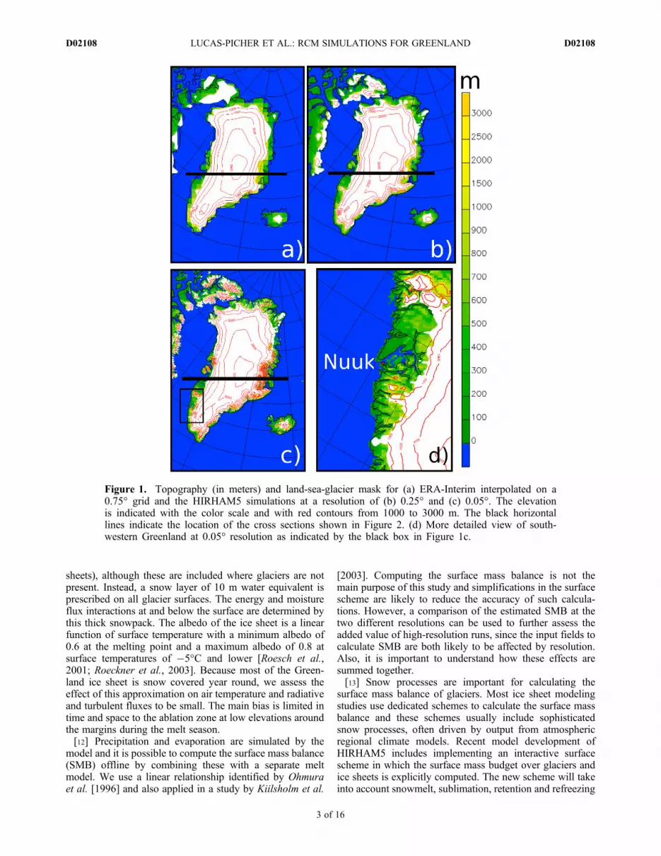
Figure 1. Topography (in meters) and land-sea-glacier mask for (a) ERA-Interim interpolated on a0.75° grid and the HIRHAM5 simulations at a resolution of (b) 0.25° and (c) 0.05°. The elevationis indicated with the color scale and with red contours from 1000 to 3000 m. The black horizontallines indicate the location of the cross sections shown in Figure 2. (d) More detailed view of south-western Greenland at 0.05° resolution as indicated by the black box in Figure 1c.


3 of 16

in the snowpack. This will allow an online coupling betweenthe RCM and an ice sheet model (R. Mottram et al., Surfacemass balance of the Greenland ice sheet 1989–2009 usingthe Regional Climate Model HIRHAM5, manuscript inpreparation, 2012).

2.2. Domain and the RCM Simulations

[14] The HIRHAM5 model is used to simulate the climateover Greenland at two horizontal resolutions, 0.05° (�5.55 km)and 0.25° (�27.75 km). The two domains are of similar sizewith 31 vertical levels and use a rotated map projection of402 � 602 and 92 � 122 grid cells to reduce grid cell dis-tortion at higher latitudes. The topography of the Greenlandice sheet is determined from the database of Bamber et al.[2001], interpolated on the HIRHAM5 grid. The twodomains and the land-sea-glacier mask are shown in Figure 1.The HIRHAM5 domain sizes and limits were chosen suchthat the whole of Greenland and Iceland are included whenthe relaxation zone has been removed. This explains why the0.25° resolution domain is larger than the one at 0.05°. Thecorresponding fields from the ERA-Interim reanalysis, inter-polated on a 0.75° rotated grid, are also shown in Figure 1a.With increasing resolution, there is a better description of thetopography and the land-sea contrast around Greenland. InFigure 1d, a small part of the southwestern coast of Greenlandat 0.05° resolution is shown in greater detail. This shows thatthe fjord systems, in this case near the capital Nuuk, are nowalmost resolved in the land-sea mask. This is not the case forthe lower-resolution representations. This is the main reasonfor our attempt to use the very high resolution.[15] Figure 2 shows a cross section of Greenland for the

two HIRHAM5 resolutions and the ERA-Interim reanalysisdata set interpolated on a 0.75° grid. The incremental rise inthe topography between two grid cells within the ablationzone is 300 to 500 m at 0.25° and even larger (�800 m) at0.75°. Such a steep increase is potentially in conflict with theformulation of the vertical structure of the climate model and

Figure 2. Cross section of Greenland and its ice sheetshowing the topography of the HIRHAM5 simulations at0.05° resolution (red line) and 0.25° resolution (blue line).The black line shows the topography used by the ERA-Interim reanalysis interpolated on a 0.75° resolution grid.The location of the cross section is indicated on Figure 1by the black lines.

Table 1. List of Stations Used for the Validation of the Simulations

Station Name Source Latitude (ºN) Longitude (ºW) Altitude (m) Time Period

Crawford Point 1 GC-Net 69.87 46.98 2022 1996–2009Crawford Point 2 GC-Net 69.90 46.85 1990 1997–2000DYE-2 GC-Net 66.47 46.27 2099 1996–2009GITS GC-Net 77.13 61.03 1869 1996–2007Humboldt GC-Net 78.52 56.82 1995 1996–2008JAR 1 GC-Net 69.48 49.70 932 1996–2009JAR 2 GC-Net 69.40 50.08 507 1999–2008JAR 3 GC-Net 69.38 50.30 283 2001–2004NASA-E GC-Net 75.00 29.98 2614 1997–2008NASA-SE GC-Net 66.47 42.48 2373 1998–2007NASA-U GC-Net 73.83 49.50 2334 1996–2008NGRIP GC-Net 75.08 42.32 2941 1997–2005Petermann GC-Net 80.68 60.28 37 2002–2006Saddle GC-Net 69.98 44.50 2901 1997–2009Swiss Camp GC-Net 69.55 49.32 1176 1996–2006South Dome GC-Net 63.13 44.82 2901 1997–2008Summit GC-Net 72.57 38.50 3199 1996–2009Tunu-N GC-Net 78.00 33.98 2052 1996–2008Aasiaat (4220) DMI 68.70 52.75 43 1989–1999Danmarkshavn (4320) DMI 76.77 18.66 11 1989–2009Illoqqortoormiut (4339) DMI 70.48 21.95 65 1989–2009Ilulissat (4221) DMI 69.22 51.05 29 1989–2009Kangerlussuaq (4231) DMI 67.02 50.70 50 1989–1999Narsarsuaq (4270) DMI 61.17 45.42 34 1989–2009Nuuk (4250) DMI 64.17 51.75 80 1989–2009Pituffik (4202) DMI 76.53 68.75 77 1989–1999P.C. Sund (4390) DMI 60.05 43.17 88 1989–1999Qaqortoq (4272) DMI 60.43 46.05 32 1989–1999Station Nord (4310) DMI 81.60 16.65 36 1989–1999Tasiilaq (4360) DMI 65.60 37.63 50 1989–2009Upernavik (4211) DMI 72.78 56.17 126 1989–2009


4 of 16

introduces systematic surface temperature errors [e.g., Dahl-Jensen et al., 2009]. The incremental rise is considerablysmaller in the 0.05° resolution simulation and does notintroduce inconsistencies. The high resolution of the RCMmay therefore contribute to accurate simulation of the tem-perature and precipitation gradients that are required for arealistic description of the surface mass balance in theablation zone. Moreover, Figure 2 shows that the models atlower resolutions than 0.05° do not depict the fjords on theeast coast of Greenland.[16] For each resolution (0.05° and 0.25°), a continuous

simulation was realized for the period 1989–2009 using theEuropean Centre for Medium-Range Weather Forecasts(ECMWF) ERA-Interim reanalysis data at T255 (�0.7°)horizontal resolution [Dee et al., 2011] as lateral boundaryconditions. The sea surface temperature and the sea ice dis-tribution from the ERA-Interim reanalysis are prescribeddaily in the model. The horizontal wind components, theatmospheric temperature, the specific humidity and the

surface pressure are transmitted to the RCM every 6 h foreach of the 31 atmospheric levels. A climate simulation at�6 km is challenging the hydrostatic assumption. Thenumerical weather prediction forecast system HIRLAM,using the same dynamical core as HIRHAM5, is used foroperational weather forecast at a few kilometers (�3–6 km)over Greenland and Denmark with satisfactory results (seehttp://www.dmi.dk/eng/index/research_and_development/dmi-hirlam-2009.htm). A comparison with a new nonhydrostaticmodel planned to be operational within a few years indicatesthat the hydrostatic assumption is not a critical limitation forthese simulations. We have therefore confidence in using themodel at this high resolution.

2.3. Weather Station Data Sets

[17] The two HIRHAM5 simulations are validated againsttwo observational data sets. The first comes from weatherstations located around the coast of Greenland, maintainedby the Danish Meteorological Institute (DMI) [Cappelenet al., 2001; Cappelen, 2010] and measuring the 2 m tem-perature and precipitation among other variables. The mea-sured precipitation can be affected by many factors such as

Figure 3. Average 2 m (a, b, c) summer (JJA) and (d, e, f)winter (DJF) temperature (in degrees Celsius) for the period1989–2009. ERA-Interim reanalysis interpolated on a 0.75°grid (Figures 3a and 3d). HIRHAM5 simulation at 0.25° res-olution (Figures 3b and 3e). HIRHAM5 simulation at 0.05°resolution (Figures 3c and 3f).

Figure 4. Average (a, b, c) summer (JJA) and (d, e, f) win-ter (DJF) precipitation (in millimeters per day) for the period1989–2009. ERA-Interim reanalysis interpolated on a 0.75°grid (Figures 4a and 4d). HIRHAM5 simulation at 0.25° res-olution (Figures 4b and 4e). HIRHAM5 simulation at 0.05°resolution (Figures 4c and 4f).


5 of 16

the wind speed and the type of precipitation [Allerup et al.,1997, 2000; Yang et al., 1999]. Therefore, the observedprecipitation used in this study has been corrected withrespect to evaporation, wetting losses and wind forcing suchas drifting snow [Wulff, 2010]. The second data set comesfrom a network of 19 automatic weather stations (AWS)distributed on the Greenland ice sheet [Steffen and Box,2001]. The AWS also measure other weather parameters,but in this study, only the temperature will be considered.Each AWS has four temperature sensors at different heights(1 and 2 m). In order to have the most consistent data set andto avoid data gaps, a mean of the four temperature sensorsfor each weather station was computed for the availableperiod. A careful inspection of the time series temperature ofthe four sensors for all the AWS was done in order toremove the temperature of sensors far from the four sensor

ensemble mean. The source, position, elevation and periodconsidered for each station is described in Table 1.

3. Validation With Observations

3.1. Spatial Distribution of Temperature andPrecipitation

[18] Figures 3 and 4 give a general impression of the cli-mate simulated by the RCM HIRHAM5 over Greenland,showing the average 2 m temperature and precipitation, forsummer (JJA) and winter (DJF), at 0.05° and 0.25° resolu-tion, respectively, during the period 1989–2009. The samevariables from the ERA-Interim reanalysis, interpolated to a0.75° grid, are also shown. The temperature from ERA-Interim is derived directly from the assimilated measure-ments, while the precipitation is simulated with the inte-grated forecast system (IFS) model. Figure 3 shows that forthe same season, the large-scale spatial distribution of the 2m temperature is similar from one resolution to another.HIRHAM5 is therefore simulating the climate realisticallyby being forced at the lateral boundaries and by the seasurface temperature from the ERA-Interim reanalysis. As theresolution increases, more details in the spatial pattern canbe observed, especially near the coast where the topographyand the land-sea mask are complex and sensitive to themodel resolution. The precipitation at the southeast coast ofGreenland during winter is more intense in the fjords and hasa higher spatial variability at 0.05° resolution (Figure 4f)than at 0.25° (Figure 4e). A more detailed analysis of theadded value of the higher-resolution simulation is presentedin section 5.

3.2. Comparison of Simulated 2 m Temperature WithData From Stations on the Coast and Ice Sheet

[19] Figure 5 presents an overview of the comparison ofthe 2 m winter (DJF) and summer (JJA) temperatures aftermatching the time periods between the RCM HIRHAM5simulations and the available data from the coastal DMIstations and the GC-Net ice sheet stations. The temperatureof the closest land grid cell is used to compare to the weatherstations and a lapse rate correction of 6°C km�1 is applied totake into account any elevation difference between theHIRHAM5 cells and the weather stations.[20] In general, the biases between the HIRHAM5 simu-

lations and the observations are between �2 and +2°C dur-ing the summer season (JJA). In winter (DJF), there is awarm bias compared to the GC-Net stations on the ice sheetand a cold bias on the southwest coast compared to the DMIstations. Figure 6 shows this opposite winter temperaturebias more clearly with a scatter diagram of the 2 m tem-peratures simulated at 0.05° and 0.25° resolution against theobservations. The correlation between the observed andsimulated values is good in summer with a small warm bias.In winter, the correlation is also good but the simulatedvalues are up to 5°C too warm for the coldest stations on theice sheet and up to 5°C too cold for the warmest stations onthe coast. There is only a small difference in the biases at0.05° and 0.25°. For spring (MAM) and fall (SON) (notshown), the biases are similar to winter with an overesti-mation of temperature on the ice sheet and an underestima-tion on the coast.

Figure 5. Temperature bias (in degrees Celsius) betweenthe HIRHAM5 simulations at 0.05° (top color cells) and0.25° (bottom color cells) resolution and observations fromDMI (blue) and GC-Net (red) stations for the period 1989–2009. The left column of color cells is for winter (DJF), andthe right column of color cells is for summer (JJA). The sta-tions JAR1, JAR2, JAR3, Swiss Camp, Crawford Point 1(CP1), and Crawford Point 2 (CP2) are not shown in theirexact locations but are presented next to each other for clarity.


6 of 16

[21] Several model specifications can contribute to thewinter warm temperature bias. The vertical resolution of themodel is too low (at standard atmosphere the lowest threemodel levels are at 33 m, 106 m, 189 m) to resolve theboundary layer processes that cause strong temperatureinversion as well as the katabatic winds, which prevail inwinter over the ice sheet. The temperature bias can also berelated to biases in the incoming longwave radiation (likelydue to errors in the cloud cover) during the dark andcloudless winter conditions and errors in the turbulentexchange near the surface, that is poorly resolved in themodel.[22] The cold bias of the HIRHAM5 simulations on the

southwest coast, compared to the DMI coastal stations, isprobably partly related to the sea ice distribution that isprescribed by the ERA-Interim reanalysis data set in theLabrador Sea and the Davis Strait. The sea ice distributionplays a critical role for the atmospheric conditions, as thesurface fluxes are dependent on whether the sea surface isice covered or not. Kauker et al. [2010] reported an over-estimation of the sea ice extent in the ERA-Interim reanal-ysis data set, which could explain the cold bias in theHIRHAM5 simulation. The model does not include frac-tional land or sea points but does allow fractional sea icecover. The model even at 0.05 degree resolution tends to bedominated by land points close to the coast, while manycoastal observational sites are mainly influenced by nearbyoceanic conditions and therefore tend to be much warmerthan just a few tens of kilometers further inland.[23] Some care should be taken when comparing a climate

variable from a grid cell, representing the mean conditionsover an area of many km2 (�6 � 6 or �28 � 28 km2 in ourcase), with a point measurement from a weather station.Climate models represent the full climate system, on thebasis of physical principles valid on large scales, and employparameterization to solve sub grid cell processes. Therefore,to validate a climate simulation, it is common to considermany grid cells over a region like a watershed or a climaticzone. In our case, high-quality gridded observations are notavailable and therefore measurements from weather stations,

that represent weather conditions at a very local scale (of afew meters), have to be considered. The local-scale mea-surements are sensitive to the immediate surrounding factorsand are thus not directly comparable to the weather condi-tions simulated by a climate model on a grid cell of manykm2. This may partly explain why the simulations do nothave smaller biases at 0.05° than at 0.25° in Figure 5 (seesection 5).

3.3. Comparison of Simulated Precipitation With DataFrom Stations on the Coast and on the Ice Sheet

[24] As with temperature, the validation of simulatedprecipitation is limited owing to the fact that there are only afew stations that measure precipitation. These stations arelocated on the coast [Cappelen, 2010] and the measuredprecipitation is affected by a number of factors. In mostcases, the measured precipitation does not reflect the“actual” precipitation. To obtain an estimate of the “actual”precipitation, the measurements have to be corrected withrespect to evaporation, wetting losses, wind speed and thetype of precipitation (snow, rain). Further details on themethod to correct the precipitation are described in the workof Wulff [2010].[25] Accumulation values measured from ice cores

[Andersen et al., 2006; Banta and McConnel, 2007; Baleset al., 2009] can be used to extend the validation of thesimulated precipitation to the whole ice sheet. Ice corederived accumulation includes deposition, sublimation, meltand snow transport by the wind. All the ice cores are takenhigh on the ice sheet where the mean temperatures are belowfreezing and melting is therefore negligible. Transport ofsnow by wind is difficult to estimate, but as the ice cores arelocated in areas with no obstacles, it is assumed that thistransport is evenly distributed. Sublimation and evaporationis estimated from the model. To make the precipitationmeasurements on the coast and the simulated precipitationcomparable to the accumulation measurements on the icesheet, the simulated evaporation is subtracted from both theobservations and the simulated precipitation.[26] Figure 7 shows the relative difference (r) (see

equation (1)) between the simulated accumulation (Asim), for

Figure 6. Simulated 2 m average temperature on (left) 0.05° and (right) 0.25° resolution against the aver-age observed temperature for the period 1989–2009. Winter (DJF) temperature is shown in blue, and sum-mer (JJA) temperature is shown in red. The observations from the DMI stations are shown with squaresand from the GC-Net stations with crosses. The slopes and the correlations of the best linear fits are indi-cated on the graph.


7 of 16

each of the closest land grid cell to the stations, and theobserved accumulation (Aobs) from both the ice cores[Andersen et al., 2006; Banta and McConnell, 2007; Baleset al., 2009] and the accumulation computed for the DMIweather stations.

r ¼ Asim � Aobs

Aobsð1Þ

The relative difference is generally closer to 0 for the 0.05°simulation than for the 0.25° simulation, especially for thehigh elevations in the center of Greenland, suggesting thehigher-resolution simulation is capturing the precipitationand evaporation better than the lower. On the southwestcoast, both simulations underestimate the accumulationwhile the other regions show both over and underestimates.

Figure 8 shows a scatter diagram of the simulated against theobserved accumulations. There is a similar correlation forthe comparison of the accumulation from the ice cores dataand the one estimated with the 0.05° and 0.25° resolutionsimulations. However, the correlation of the accumulationat the DMI weather stations and the one estimated by thesimulations is lower at 0.05° than at 0.25°. This could berelated to the high variability in precipitation between 0.05°grid cells.[27] Figure 9 shows a comparison of land-sea-glacier

mask, topography and precipitation at the two resolutions forthe region surrounding Narsarsuaq in southwest Greenland.The increase in resolution improves the description of thefjords and the topography at the coast. The more detaileddescription of the topography depicted in the 0.05° run has astrong influence on the precipitation pattern (Figure 9f). The0.05° grid cells contained within one 0.25° grid cell closestto Narsarsuaq show a large variability of precipitation.Figure 10 shows the average 1989–2009 monthly meanprecipitation for the 0.05° and 0.25° grid cell closest to theNarsarsuaq station and the seven 0.05° neighboring land gridcells. The simulated precipitation can double or even triplefrom one grid cell to another. Figure 10 also shows the uncor-rected and corrected precipitation measurements at the DMIstation Narsarsuaq (4270). The correction factor for the pre-cipitation is close to two in the winter months. The simulatedprecipitation at the closest 0.05° grid cell is considerably higherthan the corrected measured values. However, the comparisonis better at a few of the neighboring grid cells. The height of theclosest and neighboring 0.05° grid cells varies from 124 to622 m. This is far from the elevation of the station at 34 m.The neighboring 0.05° cell with the lowest elevation is notthe one, which shows the closest time series to the observa-tions. The large cell-to-cell variability amply demonstrateswhy validation is difficult for the precipitation on the coast ofGreenland. The precipitation field in the interior of Greenlandhas a smaller cell-to-cell variability than on the coast.Therefore, more confidence should be put on the precipita-tion validation over the ice sheet.

4. Description of the Simulated ClimateOver Greenland

[28] The model validation presented above confirms thatthe RCM HIRHAM5 is doing a fair job simulating the 2 mtemperature and precipitation over Greenland. These simu-lations can therefore be used to describe the climate overGreenland, which is to a large extent unknown due the smallamount of in situ observations. To examine the regionalvariability, four regions are defined on the basis of the sur-face topography of the Greenland ice sheet [Bamber et al.,2001]. Ice sheet drainage basins were determined using themethod described by Schwanghart and Kuhn [2010] and thelocation of the major outlet glaciers identified [Hardy andBamber, 2000]. The resulting nine drainage basins werelater joined together according to the similarities in theirclimate to form the final four drainage basis shown inFigure 11a.[29] Region 1 covers the north of Greenland with cold

(<�30°C) and dry (<0.5 mm d�1) winters as shown inFigures 11b and 11c. Region 2 on the southeast coast has a

Figure 7. Relative difference (r; see equation (1)) betweenthe HIRHAM5 simulated accumulation at 0.05° (small cir-cle) and 0.25° (large circle) resolution and the observedaccumulation from ice core measurements and the DMIweather stations.


8 of 16

milder climate with wet conditions, especially in the winter.Region 3 located on the southern tip of Greenland presentsthe warmest conditions with an annual mean 2 m tempera-ture around �10°C and wet conditions (>4 mm d�1 annu-ally), with higher precipitation in the winter. Region 4, on

the west coast, is cold and dry with wetter conditions in thesummer and autumn. Similar analysis for the whole ofGreenland including land points not covered with ice, aswell as the surrounding sea is shown in Figure 11.

Figure 8. Simulated average accumulation at (a) 0.05° and (b) 0.25° resolution against the averageobserved accumulation for the period 1989–2009. The observations from ice cores are shown in red,and observations from the DMI stations are shown in blue. The slopes and the correlations for the best lin-ear fits are indicated on the graph.

Figure 9. Comparison of (a and d) land-sea-glacier mask (sea in blue, land in green, glacier in white);(b and e) topography (in meters); and (c and f) the 1989–2009 winter (DJF) precipitation (millimetersper day) simulated with HIRHAM5 at a resolution of 0.25° (Figures 9a–9c) and 0.05° (Figures 9d–9f).The closest 0.05° and 0.25° grid cells to the DMI station Narsarsuaq are shown with a red and blacksquares, respectively.


9 of 16

[30] The mean annual temperature and precipitation sim-ulated with HIRHAM5 at 0.05° are shown in Figures 12aand 12b, respectively. Region 1 in the north shows thestrongest warming trend with a mean annual increase of0.11°C yr�1 (significant above the 99% significance levelaccording to a two-tailed t test). The other regions showlower positive trends for the temperature, also significantabove 99%. The precipitation trends are weak and not sig-nificant (above 99%) according to a two-tailed t test. Thetrends of the 0.05° simulation are not statistically differentfrom those of the 0.25° simulation and do not reflect anyadded value. The mean temperature and the warming trenddetermined by HIRHAM5 for the ERA-Interim period overGreenland are consistent with those reported by other modelstudies including Fettweis [2007], Box et al. [2009], andEttema [2010].[31] In Figure 13, the analysis of the mean annual tem-

perature and precipitation is extended to examine whetherdifferent elevation bands of Greenland have evolved differ-ently during the period 1989–2009. The results indicate thatthe lower elevations (0–1000 m) have warmed the mostduring the period 1989–2009, with a linear trend of 0.13°Cyr�1. The temperature trends decrease toward the higherelevations. All trends for the temperature are significantabove 99% according to a two-tailed t test. For the precipi-tation, the trends are weak and not significant. Moreover, itis interesting to notice the strong temporal correlation

Figure 10. Simulated mean monthly precipitation fromHIRHAM5 at 0.05° resolution for the period 1989–2009 atthe closest grid cell to the DMI station Narsarsuaq (station4270; thick black line) and its seven neighboring land gridcells (gray lines). The corresponding values for the closestgrid cell of HIRHAM5 at 0.25° are indicated in green. Theuncorrected and corrected observed precipitation measure-ments at Narsarsuaq are shown in red and blue, respectively.

Figure 11. (a) Division of the Greenland ice sheet into four drainage regions. (b) Mean monthly 2 m tem-perature (in degrees Celsius) and (c) the mean monthly precipitation (in millimeters per day) for the fourregions (all Greenland and all ocean cells are shown in Figure 11a) averaged over the period 1989–2009for the 0.05° HIRHAM5 simulation. The numbers in the graphs show the annual mean temperature andprecipitation for each region.


10 of 16

between the 2 m temperature and the precipitation inFigures 13a and 13b. A warm year has generally strongerprecipitation than a cold year.

5. Impact of Higher Resolution: Assessmentof Added Value

[32] The comparison of the model output at the two reso-lutions with observations in section 3 shows that the precip-itation and temperature biases do not decrease significantlywith increased resolution. However, the validation is notcomprehensive owing to the few available observations, theirshort duration and the inherent measurement errors, espe-cially the precipitation measurements, which have to becorrected for various factors. For a more robust comparisonbetween the two simulations and to assess the added value ofthe higher resolution, the two HIRHAM5 simulations arecompared directly to one another.[33] Figure 14 shows the difference of the elevation, the

1989–2009 mean annual 2 m temperature, precipitation andcloud cover between the 0.05° and 0.25° simulations. Here, nocorrection was done on the temperature to take into account

the different heights. With higher resolution, the elevation ofthe small mountains on the coast of Greenland is generallyhigher than at lower resolution. Consequently, the 0.05° sim-ulation is mainly colder and wetter on the coast of Greenlandcompared to the 0.25° simulation. The increase in resolutionallows a better description of the topography, which increasesthe orographically enhanced precipitation on the coast. Theincrease in precipitation on the coast of Greenland at 0.05°compared to 0.25° resolution simulation dries out the atmo-sphere and may explain the lower cloud cover at 0.05° gen-erating less precipitation. The colder conditions over the mainice sheet at 0.05° are mainly linked to the reduced downwardlongwave radiation at the surface associated to the lower cloudcover for the higher-resolution simulation.[34] This effect is shown more clearly in Figure 15, which

shows a cross section of the 1989–2009 2 m temperature andprecipitation for the summer months June, July and August(JJA). Figure 15b shows that the maximum precipitation onthe west coast of Greenland is located closer to the ice sheetedge at 0.05° than at 0.25°. This leads to drier and colderconditions at higher elevations for the simulation at higherresolution. Figure 15 also shows the difference between the

Figure 12. Mean annual (a) 2 m temperature (in degrees Celsius) and (b) precipitation (in millimetersper day) for the period 1989–2009 for the four drainage regions (all Greenland and all ocean cells areshown in Figure 11a) for the 0.05° HIRHAM5 simulation. The numbers in the graphs show the 21 yearaverage and the trend for this period.

Figure 13. Mean annual (a) 2 m temperature (in degrees Celsius) and (b) precipitation (in millimetersper day) for the period 1989–2009 for different height bins of 500 m for the 0.05° HIRHAM5 simulationover Greenland. The numbers in the graphs show the 21 year average and the trend for this period.


11 of 16

two simulations on the east side of Greenland where thetopography is sensitive to the resolution (see also Figure 2).[35] Further to this, we show in Figure 15c the surface

mass balance calculated offline using annual snow fall andevaporation, plus summer temperature output from the tworuns. To estimate ablation, we use an empirical relationship[Ohmura et al., 1996; Kiilsholm et al., 2003] between theannual loss of mass and the seasonal mean air temperatureabove �2°C for June, July and August. A summer meantemperature of �2°C is the minimum temperature wheremass loss due to ablation can be expected and a linear rela-tion for the trend has been calculated on basis of observa-tions by Ohmura et al. [1996] andWild and Ohmura [2000].Refreezing at the surface is taken into account by this

method, although the complete physical understanding ofthe relationship behind it is not fully accounted for. With aresolved topographical gradient near the ice edge, the abla-tion zone is well constrained. Note for example that within afew tens of kilometers from the ice sheet margin, the altitudejump between neighboring grid points is on the order of ahundred meters even at 0.05° resolution. This influences theSMB quite substantially as both the local ablation and pre-cipitation is strongly altitude dependent. As a result, thelocal SMB on the western part of the ice sheet in this crosssection is reduced in the higher-resolution experiment com-pared to the coarser one with a similar pattern on the eastcoast, likely reflecting the precipitation pattern shown inFigure 15b. Despite comparable performance between the

Figure 14. Difference over Greenland between the HIRHAM5 simulations at 0.05° and 0.25° for (a) eleva-tion (meters), (b) 1989–2009 mean 2 m temperature (in degrees Celsius), (c) 1989–2009 mean precipitation(in millimeters per day) and (d) 1989–2009 mean cloud fraction [0,1]. The inner black contour indicates thelimit of the ice sheet at 0.25°.


12 of 16

Figure 15. Cross sections of the 1989–2009 summer (JJA) (a) 2 m temperature (in degrees Celsius),(b) precipitation (in millimeters per day), and (c) offline estimate of the surface mass balance (SMB)(in millimeters per year). The simulated values at 0.05° and 0.25° are shown in red and blue, respectively.The topography of Greenland at 0.05° is shown with a black line. The location of the cross section is indi-cated on Figure 1.

Figure 16. Elevation dependency of the HIRHAM5 simulated (a) 2 m temperature (in degrees Celsius)and (b) precipitation (in millimeters per day) at 0.05° (red) and 0.25° (blue) using 200 m bins over Green-land. The same fields for the ERA-Interim reanalysis are presented in green. The numbers in the graphscorrespond to the average over all the levels.


13 of 16

two experiments (0.05 and 0.25° resolution) when validatedagainst station data, we therefore assess that the higher res-olution gives the best estimate of the true SMB.[36] The impact of the resolution over the whole ice

sheet is shown in Figure 16 where the elevation dependencyof the 2 m temperature and the precipitation for the twoHIRHAM5 simulations and ERA-Interim reanalysis is pre-sented. Figure 16b shows that below 1200 m, the simulationat 0.05° is generating more precipitation than the simulationat 0.25°. This is probably due to the steeper slopes at 0.05°resolution that increase the precipitation amount due to theorographic enhancement. Above 1200 m, the opposite isobserved. The 0.25° simulation has more precipitation thanthe 0.05° simulation. This is mainly caused by wetter andwarmer atmospheric conditions in the 0.25° resolution sim-ulation compared to the simulation at 0.05°, which loses mostof the atmospheric moisture at the ice sheet edges as dis-cussed. As indicated in Figure 16b, it is interesting to notethat the mean precipitation over Greenland is larger at 0.25°(1.42 mm d�1) than at 0.05° (1.37 mm d�1). This may beassociated with the fact that more precipitation is falling overthe ocean rather than on the land in the 0.05° resolution sim-ulation owing to the larger topographic gradients. On the icesheet, the drier conditions and the higher elevation of the0.05° simulation also lead to lower temperatures (Figure 16a).[37] The total amount of precipitation simulated with

HIRHAM5 at 0.05° and 0.25° resolutions over the whole ofGreenland, including land points not covered with ice, isalmost the same for both (3% difference; see Figure 17).However, the total amount of precipitation simulated overthe ice sheet only is 11% larger at 0.25° than at 0.05°. Moreprecipitation is simulated with the 0.05° resolution model atthe coast of Greenland owing to the steeper slopes. The totalamount of precipitation over the Greenland ice sheet in theyear 1992 computed with HIRHAM5 at 0.05° (753� 1012 kg)and 0.25° (856 � 1012 kg) is in close agreement with thatcomputed by Ettema et al. [2009] with the RCM RACMO2

at 0.1° (�757 � 1012 kg) and 0.15° (�729 � 1012 kg). Theconclusion of Ettema et al. [2009], that more mass accumu-lates on the Greenland ice sheet with higher resolution, is notsupported by the comparison of the 0.25° and 0.05° resolu-tion simulations with HIRHAM5. In the HIRHAM5model, itappears that the orographically enhanced precipitation redu-ces the amount of moisture over the main ice sheet andthereby reduces the total amount of precipitation for thehigher-resolution simulation.

6. Discussions and Conclusions

[38] A robust validation of two 1989–2009 HIRHAM5simulations (0.05° and 0.25° resolution) over Greenlandusing the ERA-Interim reanalysis as lateral boundary con-ditions is presented. The model output is compared withobserved 2 m temperature and precipitation from the DMImeteorological stations on the coast and the GC-Net auto-matic weather stations on the ice sheet. The simulated 2 mtemperature is in good agreement with observations overGreenland in summer, while in winter the temperature islower than observed in the southwest and higher at higherelevations of the ice sheet. The increase in resolution from0.25° to 0.05° does not reduce the temperature bias for theweather stations on the coast and on the ice sheet. This is inagreement with the study of Mass et al. [2002], who foundno significant improvement of the objectively scored accu-racy of the forecasts as the grid spacing decrease to less than10–15 km. A high-quality 2 m gridded temperature fieldbased on observations over Greenland would be necessary toassess whether a higher-resolution model improves thetemperature simulation. The accumulation bias is reducedwith higher resolution at the higher elevation on the ice sheetwhere the precipitation field is homogeneous. On the coastof Greenland, the increase in resolution increases the spatialvariability of the topography, which has a strong impact onthe simulated precipitation. Therefore, it is not feasible tomake a fair comparison to the point measurements when thespatial variability in the model output is so large.[39] An analysis of the simulated climate over Greenland

for the period 1989–2009 shows that the largest warmingtrend is in the north of Greenland where the climate is dryand cold. Moreover, the warming trend is larger at lowerelevations than at higher elevations. No significant trends forthe precipitation were found for the different regions orheight intervals during the period 1989–2009. Direct com-parison of the HIRHAM5 simulations at 0.05° and 0.25°resolution shows that the 0.05° simulation is significantlywetter close to the coast and drier at high elevations than the0.25° simulation. Also, the 0.05° simulation has less pre-cipitation than the 0.25° simulation in the ablation zonewhere the highest relief is found. This could have importantconsequences when the climate outputs are given to an icesheet model.[40] This study shows the usefulness of the high-resolu-

tion regional climate model simulation for ice sheet studiesas the high spatial variability is not captured in the low-resolution driving model. With the higher-resolution simu-lation, the description of the climate fields over Greenlandappears to be more physically plausible owing to the addi-tional details in the precipitation and temperature patternssimulated at the margins of the ice sheet where most of the

Figure 17. Total precipitation summed (GT per year) overall Greenland (thin lines) and over the Greenland ice sheet(thick lines) for the two HIRHAM5 simulations for theperiod 1989–2009 (0.05° resolution in red; 0.25° in blue);ERA-Interim is shown in green. The numbers in the graphindicate the 21 year mean total precipitation for HIRHAM5at 0.05° and 0.25° and ERA-Interim over the ice sheet andover all Greenland.


14 of 16

ablation occurs. A good description of the climate of theablation zone is critical when calculating surface mass bal-ance for the full ice sheet and when coupling climate modelsto ice sheet models in order to simulate realistically thecurrent and future responses of the Greenland ice sheet toclimate change.[41] A number of improvements are currently planned,

including adding the computation of the surface mass bal-ance within the RCM for which more realistic snow pro-cesses are required. Along with such improvements, a bettertreatment of the surface processes is planned, which willimprove the radiative balance on the ice sheet surface, byincluding a correct snowmelt scheme, an improved albedoscheme and allowing the melting of glacier ice (R. Mottramet al., manuscript in preparation, 2012).[42] This study provides baseline high-resolution simula-

tions of the recent climate of Greenland. The small biases inthe simulations show that HIRHAM5 generates a realisticclimate over Greenland, which is suitable to drive ice sheetmodels. These results illustrate that the dynamical down-scaling of reanalysis is necessary to correctly characterizethe climate of Greenland at the regional scale. Furthermore,these results underline the sensitivity to the model resolu-tion. Additionally, this study highlights both the difficultiesthat the lack of observations pose for validation of RCMsand the advantages of using an RCM in areas where obser-vations are sparse in order to create a regional climatology.RCMs allow us to make projections of future climate on aregional scale, but also to study the immediate causes andeffects of those climate changes. The output of those simu-lations will be used to drive ice sheet models participating inthe project ice2sea. The response of the ice sheet models tothe climate forcing from the RCM will give additionalinformation on the accuracy of the climate simulated by theRCMs.

[43] Acknowledgments. We acknowledge the ice2sea project fundedby the European Commission’s 7th Framework Programme through grant226375. This is ice2sea manuscript 034. In addition, this study was partiallysupported by the Greenland Climate Research Center (project 6504).

ReferencesAhlstrøm, A. P., et al. (2008), A new programme for monitoring the massloss of the Greenland ice sheet, Geol. Surv. Den. Greenl. Bull., 15, 61–64.

Allerup, P., H. Madsen, and F. Vejen (1997), A comprehensive model forcorrecting point precipitation, Nord. Hydrol., 28, 1–20.

Allerup, P., H. Madsen, and F. Vejen (2000), Correction of observed pre-cipitation in Greenland, paper presented at XXI Nordic HydrologicalConference, Nord. Assoc. for Hydrol., Uppsala, Sweden, 26–30 June.

Andersen, K. K., P. D. Ditlevsen, S. O. Rasmussen, H. B. Clausen, B. M.Vinther, S. J. Johnsen, and J. P. Steffensen (2006), Retrieving a commonaccumulation record from Greenland ice cores for the past 1800 years,J. Geophys. Res., 111, D15106, doi:10.1029/2005JD006765.

Aðalgeirsdóttir, G., M. Stendel, J. H. Christensen, J. Cappelen, F. Vejen,H. A. Kjær, R. Mottram, and P. Lucas-Picher (2009), Assessment of thetemperature, precipitation and snow in the RCM HIRHAM4 at 25 kmresolution, Clim. Cent. Rep. 09-08, Dan. Meteorol. Inst., Copenhagen.[Available at http://www.dmi.dk/dmi/dkc09-08.pdf.]

Bales, R. C., Q. Guo, D. Shen, J. R. McConnell, G. Du, J. F. Burkhart, V. B.Spikes, E. Hanna, and J. Cappelen (2009), Annual accumulation forGreenland updated using ice core data developed during 2000–2006and analysis of daily coastal meteorological data, J. Geophys. Res., 114,D06116, doi:10.1029/2008JD011208.

Bamber, J. L., S. Ekholm, and W. B. Krabill (2001), A new, high-resolutiondigital elevation model of Greenland fully validated with airborne laseraltimeter data, J. Geophys. Res., 106, 6733–6745, doi:10.1029/2000JB900365.

Banta, J. R., and J. R. McConnell (2007), Annual accumulation over recentcenturies at four sites in central Greenland, J. Geophys. Res., 112,D10114, doi:10.1029/2006JD007887.

Box, J. E., and A. Rinke (2003), Evaluation of Greenland ice sheet surfaceclimate in the HIRHAM regional climate model using automatic weatherstation data, J. Clim., 16, 1302–1319, doi:10.1175/1520-0442-16.9.1302.

Box, J. E., L. Yang, D. H. Bromwich, and L.-S. Bai (2009), GreenlandIce Sheet surface air temperature variability: 1840–2007, J. Clim., 22,4029–4049, doi:10.1175/2009JCLI2816.1.

Burgess, E. W., R. R. Forster, J. E. Box, E. Mosley-Thompson, D. H.Bromwich, R. C. Bales, and L. C. Smith (2010), A spatially calibratedmodel of annual accumulation rate on the Greenland Ice Sheet (1958–2007), J. Geophys. Res., 115, F02004, doi:10.1029/2009JF001293.

Cappelen, J. (Ed.) (2010), DMI monthly climate data collection, 1768–2009:Denmark, the Faroe Islands and Greenland, Tech. Rep. 10-05, Dan.Meteorol. Inst., Copenhagen. [Available at http://www.dmi.dk/dmi/tr10-05.pdf.]

Cappelen, J., B. V. Jørgensen, E. V. Laursen, L. S. Stannius, and R. S.Thomsen (2001), The observed climate of Greenland, 1958–1999, withclimatological standard normals, 1961–1990, Tech. Rep. 00-18, Dan.Meteorol. Inst., Copenhagen. [Available at http://www.dmi.dk/dmi/tr00-18.pdf.]

Christensen, O. B., M. Drews, J. H. Christensen, K. Dethloff, K. Ketelsen,I. Hebestadt, and A. Rinke (2006), The HIRHAM regional climatemodel, version 5, Tech. Rep. 06-17, Dan. Meteorol. Inst., Copenhagen.[Available at http://www.dmi.dk/dmi/tr06-17.pdf.]

Dahl-Jensen, D., et al. (2009), The Greenland Ice Sheet in a changingclimate: Snow, Water, Ice and Permafrost in the Arctic (SWIPA), report,115 pp., Arctic Monit. and Assess. Programme, Oslo. [Available at http://www.amap.no/swipa/press2009/GRISindex.html.]

Davies, H. C. (1976), A lateral boundary formulation for multi-level predic-tion models, Q. J. R. Meteorol. Soc., 102, 405–418.

Dee, D. P., et al. (2011), The ERA-Interim reanalysis: Configuration andperformance of the data assimilation system, Q. J. R. Meteorol. Soc.,137, 553–597, doi:10.1002/qj.828.

Dümenil, L., and E. Todini (1992), A rainfall–runoff scheme for use in theHamburg climate model, in Advances in Theoretical Hydrology, Eur.Geophys. Ser. Hydrol. Sci., vol. 1, edited by J. P. O’Kane, pp. 129–157,Elsevier, New York.

Eerola, K. (2006), About the performance of HIRLAM version 7.0,HIRLAM Newsl., 51, 93–102.

Ettema, J. (2010), The present day climate of Greenland: A study with aregional climate model, PhD thesis, Univ. of Utrecht, Utrecht,Netherlands.

Ettema, J., M. R. van den Broeke, E. van Meijgaard, W. J. van de Berg, J. L.Bamber, J. E. Box, and R. C. Bales (2009), Higher surface mass balanceof the Greenland ice sheet revealed by high-resolution climate modeling,Geophys. Res. Lett., 36, L12501, doi:10.1029/2009GL038110.

Ettema, J., M. R. van den Broeke, E. van Meijgaard, W. J. van de Berg, J. E.Box, and K. Steffen (2010), Climate of the Greenland ice sheet usinga high-resolution climate model—Part 1: Evaluation, Cryosphere, 4,511–527, doi:10.5194/tc-4-511-2010.

Fettweis, X. (2007), Reconstruction of the 1979–2006 Greenland icesheet surface mass balance using the regional climate model MAR,Cryosphere, 1, 21–40, doi:10.5194/tc-1-21-2007.

Giorgi, F. (2006), Regional climate modeling: Status and perspectives,J. Phys. IV, 139, 101–118, doi:10.1051/jp4:2006139008.

Hardy, R. J., and J. L. Bamber (2000), The delineation of drainage basins onthe Greenland ice sheet for mass-balance analyses using a combined mod-elling and geographical information system approach, Hydrol. Process.,14, 1931–1941, doi:10.1002/1099-1085(20000815/30)14:11/12<1931::AID-HYP46>3.0.CO;2-2.

Kauker, K., R. Gerdes, M. Karcher, T. Kaminski, R. Giering, and M. Vossbeck(2010), June 2010 Sea Ice Outlook–AWI/FastOpt/OASys contribution,report, Arctic Res. Consortium of the U.S., Fairbanks, Alaska. [Availableat http://www.arcus.org/files/search/sea-ice-outlook/2010/06/pdf/pan-arc-tic/kaukeretaljuneoutlook.pdf.]

Kiilsholm, S., J. H. Christensen, K. Dethloff, and A. Rinke (2003), Netaccumulation of the Greenland ice sheet: High resolutionmodeling of climatechanges, Geophys. Res. Lett., 30(9), 1485, doi:10.1029/2002GL015742.

Luthcke, S. B., H. J. Zwally, W. Abdalati, D. D. Rowlands, D. R. Ray, R. S.Nerem, G. G. Lemoine, J. J. McCarthy, and D. S. Chinn (2006), RecentGreenland ice mass loss by drainage system from satellite gravity obser-vations, Science, 314, 1286–1289, doi:10.1126/science.1130776.

Mass, C. F., D. Ovens, K. Westrick, and B. A. Colle (2002), Does increas-ing horizontal resolution produce more skilled forecasts? The results oftwo years of real-time numerical weather prediction over the PacificNorthwest, Bull. Am. Meteorol. Soc., 83, 407–430, doi:10.1175/1520-0477(2002)083<0407:DIHRPM>2.3.CO;2.


15 of 16

Nordeng, T. E. (1994), Extended versions of the convective parameteriza-tion scheme at ECMWF and their impact on the mean and transient activ-ity of the model in the tropics, Tech. Memo. 206, 41 pp., Eur. Cent. forMed. Range Weather Forecasts, Reading, U. K.

Ohmura, A., M. Wild, and L. Bengtsson (1996), A possible change in massbalance of Greenland and Antarctic ice sheets in the coming century,J. Clim., 9, 2124–2135, doi:10.1175/1520-0442(1996)009<2124:APCIMB>2.0.CO;2.

Pritchard, H. D., R. J. Arthern, D. G. Vaughan, and L. A. Edwards (2009),Extensive dynamic thinning on the margins of the Greenland and Antarc-tic ice sheets, Nature, 461, 971–975, doi:10.1038/nature08471.

Randall, D. A., et al. (2007), Climate models and their evaluation, in Cli-mate Change 2007: The Physical Science Basis. Contribution of WorkingGroup I to the Fourth Assessment Report of the Intergovernmental Panelon Climate Change, edited by S. Solomon et al., pp. 591–662, CambridgeUniv. Press, New York.

Roeckner, E., et al. (2003), The atmospheric general circulation modelECHAM5. Part 1. Model description, Rep. 349, Max-Planck-Inst. forMeteorol., Hamburg, Germany. [Available at www.mpimet.mpg.de/fileadmin/publikationen/Reports/max_scirep_349.pdf.]

Roesch, A., M. Wild, H. Gilgen, and A. Ohmura (2001), A new snowcover fraction parameterization for the ECHAM4 GCM, Clim. Dyn.,17, 933–946, doi:10.1007/s003820100153.

Schwanghart, W., and N. J. Kuhn (2010), TopoToolbox: A set of Matlabfunctions for topographic analysis, Environ. Modell. Software, 25, 770–781,doi:10.1016/j.envsoft.2009.12.002.

Sørensen, L. S., S. B. Simonsen, K. Nielsen, P. Lucas-Picher, G. Spada,G. Adalgeirsdottir, R. Forsberg, and C. S. Hvidberg (2011), Mass balanceof the Greenland ice sheet (2003–2008) from ICESat data—The impact ofinterpolation, sampling and firn density, Cryosphere, 5, 173–186,doi:10.5194/tc-5-173-2011.

Steffen, K., and J. E. Box (2001), Surface climatology of the Greenland icesheet: Greenland Climate Network 1995–1999, J. Geophys. Res., 106,33,951–33,964, doi:10.1029/2001JD900161.

Stendel, M., J. H. Christensen, G. Aðalgeirsdóttir, N. Kliem, and M. Drews(2007), Regional climate change for Greenland and surrounding seas.Part I: Atmosphere and land surface, Clim. Cent. Rep. 07-02, Dan.Meteorol. Inst., Copenhagen. [Available at http://www.dmi.dk/dmi/dcc07-02.pdf.]

Sundqvist, H. (1978), A parameterization scheme for non-convectivecondensation including precipitation including prediction of cloudwater content, Q. J. R. Meteorol. Soc., 104, 677–690, doi:10.1002/qj.49710444110.

Tiedtke, M. (1989), A comprehensive mass flux scheme for cumulus param-eterization in large-scale models, Mon. Weather Rev., 117, 1779–1800,doi:10.1175/1520-0493(1989)117<1779:ACMFSF>2.0.CO;2.

van de Wal, R. S. W., W. Greuell, M. R. van den Broeke, C. H. Reijmer,and J. Oerlemans (2005), Surface mass-balance observations and automaticweather station data along a transect near Kangerlussuaq, west Greenland,Ann. Glaciol., 42, 311–316, doi:10.3189/172756405781812529.

Velicogna, I. (2009), Increasing rates of ice mass loss from the Greenlandand Antarctic ice sheets revealed by GRACE, Geophys. Res. Lett., 36,L19503, doi:10.1029/2009GL040222.

Wild, M., and A. Ohmura (2000), Change in mass balance of polar icesheets and sea level from high-resolution GCM simulation of greenhousewarming, Ann. Glaciol., 30, 197–203, doi:10.3189/172756400781820741.

Wulff, M. (2010), Empirical correction of simulated accumulation overGreenland, 136 pp., MS thesis, Niels Bohr Inst., Univ. of Copenhagen,Copenhagen. [Available at http://www.nbi.ku.dk/english/Calendar/activities_10/master_thesis_28052079/Maria_wulff.pdf.]

Yang, D., S. Ishida, B. E. Goodison, and T. Gunther (1999), Bias correctionof daily precipitation measurements for Greenland, J. Geophys. Res., 104,6171–6181, doi:10.1029/1998JD200110.

Zwally, H. J., et al. (2011), Greenland ice sheet mass balance: Distributionof increased mass loss with climate warming: 2003–07 versus 1992–2002,J. Glaciol., 57, 88–102, doi:10.3189/002214311795306682.

G. Aðalgeirsdóttir, J. H. Christensen, and R. Mottram, DanishMeteorological Institute, Lyngbyvej 100, DK-2100 Copenhagen, Denmark.P. Lucas-Picher, Centre National de Recherches Météorologiques,

Météo-France, 42 Av. Gaspard Coriolis, F-31057 Toulouse, France.([email protected])S. B. Simonsen, Centre for Ice and Climate, Niels Bohr Institute,

University of Copenhagen, Juliane Maries vej 30, DK-2100 Copenhagen,Denmark.M. Wulff-Nielsen, Planetary Physics and Geophysics, Niels Bohr

Institute, University of Copenhagen, DK-2100 Copenhagen, Denmark.


16 of 16

Documents

Very high resolution regional climate model simulations over Greenland: Identifying added value