A SIMPLE based discontinuous Galerkin solver for steady incompressible flows

Journal of Computational Physics 237 (2013) 235–250

Contents lists available at SciVerse ScienceDirect

Journal of Computational Physics

journal homepage: www.elsevier .com/locate / jcp

A SIMPLE based discontinuous Galerkin solver for steadyincompressible flows

0021-9991/$ - see front matter � 2012 Elsevier Inc. All rights reserved.http://dx.doi.org/10.1016/j.jcp.2012.11.051

⇑ Corresponding author at: Chair of Fluid Dynamics, Department of Mechanical Engineering, Technische Universität Darmstadt, Petersenstr. 3Darmstadt, Germany. Tel.: +49 6151 16 70955; fax: +49 6151 16 7061.

E-mail addresses: [email protected] (B. Klein), [email protected] (F. Kummer), [email protected] (M. Oberla

Benedikt Klein a,b,c,⇑, Florian Kummer a,c, Martin Oberlack a,b,c

a Chair of Fluid Dynamics, Department of Mechanical Engineering, Technische Universität Darmstadt, Petersenstr. 30, 64287 Darmstadt, Germanyb Center of Smart Interfaces, Technische Universität Darmstadt, Petersenstr. 32, 64287 Darmstadt, Germanyc Graduate School of Computational Engineering, Technische Universität Darmstadt, Dolivostr. 15, 64293 Darmstadt, Germany

a r t i c l e i n f o

Article history:Received 6 February 2012Received in revised form 26 October 2012Accepted 26 November 2012Available online 14 December 2012

Keywords:Finite element methodsDiscontinuous Galerkin methodsNavier–Stokes equationsIncompressible flowsSegregated solution algorithmsSIMPLE algorithm

a b s t r a c t

In this paper we present how the well-known SIMPLE algorithm can be extended to solvethe steady incompressible Navier–Stokes equations discretized by the discontinuous Galer-kin method. The convective part is discretized by the local Lax-Friedrichs fluxes and theviscous part by the symmetric interior penalty method. Within the SIMPLE algorithm,the equations are solved in an iterative process. The discretized equations are linearizedand an equation for the pressure is derived on the discrete level. The equations obtainedfor each velocity component and the pressure are decoupled and therefore can be solvedsequentially, leading to an efficient solution procedure. The extension of the proposedscheme to the unsteady case is straightforward, where fully implicit time schemes canbe used.

Various test cases are carried out: the Poiseuille flow, the channel flow with constanttranspiration, the Kovasznay flow, the flow into a corner and the backward-facing stepflow. Using a mixed-order formulation, i.e. order k for the velocity and order k� 1 forthe pressure, the scheme is numerically stable for all test cases. Convergence rates ofkþ 1 and k in the L2-norm are observed for velocity and pressure, respectively. A studyof the convergence behavior of the SIMPLE algorithm shows that no under-relaxation forthe pressure is needed, which is in strong contrast to the application of the SIMPLE algo-rithm in the context of the finite volume method or the continuous finite element method.We conclude that the proposed scheme is efficient to solve the steady incompressibleNavier–Stokes equations in the context of the discontinuous Galerkin method comprisinghp-accuracy.

� 2012 Elsevier Inc. All rights reserved.

1. Introduction

When simulating incompressible flows the finite volume method (FVM) and the finite element method (FEM) are widelyused. Besides, a newer method is becoming more popular, namely the discontinuous Galerkin method (DGM). The discon-tinuous Galerkin method comprises favorable properties of both the finite volume and the finite element method. In the con-text of the DGM, physical quantities are approximated by polynomials on each cell of the numerical grid (similar to FEM),where the approximation is discontinuous across the element interfaces (similar to FVM). Discontinuous Galerkin methodsare highly accurate, the order of the approximating polynomials can be arbitrarily chosen, and they are geometrically flexibleat the same time.

0, 64287

ck).

http://crossmark.dyndns.org/dialog/?doi=10.1016/j.jcp.2012.11.051&domain=pdf

http://dx.doi.org/10.1016/j.jcp.2012.11.051

mailto:[email protected]



http://dx.doi.org/10.1016/j.jcp.2012.11.051

http://www.sciencedirect.com/science/journal/00219991

http://www.elsevier.com/locate/jcp

236 B. Klein et al. / Journal of Computational Physics 237 (2013) 235–250

The application of the DG method to the steady and unsteady incompressible Navier–Stokes equations has recently beenreported by several authors. For the steady case, Cockburn et al. [1] developed the local discontinuous Galerkin method(LDG). Rivière and Girault [2] compared the symmetric and non-symmetric interior penalty method. In both approaches([1,2]) a fixed point iteration is used to solve the resulting non-linear discrete system, i.e. velocity and pressure are solvedin a fully coupled manner. For the unsteady case, Girault et al. [3] also used the symmetric and non-symmetric interior pen-alty method together with a differential splitting technique. Bassi et al. [4] developed a special flux for the transport termbased on the solution of local Riemann problems by introducing an artificial compressibility perturbation, while time march-ing is done by implicit Runge–Kutta schemes. The schemes proposed by Shahbazi et al. [5] and Ferrer and Willden [6] employalgebraic and differential splitting techniques, respectively, where the convective part is treated explicitly and the viscouspart is treated implicitly. In [5] the convective term is discretized by the local Lax-Friedrichs fluxes and in [6] by a modifiedformulation of the Lesaint–Raviart fluxes. Again, in both schemes the symmetric interior penalty method is used for the vis-cous part.

Independently of the DG discretization, there are some difficulties when simulating incompressible flows: (i) the equa-tions are non-linear due to the convective part; (ii) velocity and pressure are strongly coupled via an elliptic operator;(iii) an explicit equation to calculate the pressure is missing. The solution techniques found in the context of the DG methodin the references [1–6] can be divided into three groups:

(a) fixed point iteration for steady cases, solving the non-linear system for all velocity components and the pressure in afully coupled manner [1,2];

(b) operator splitting techniques for unsteady cases, either at the algebraic or differential level [3,5,6];(c) implicit Runge–Kutta schemes of the Rosenbrock-type, where (like in group (a)) all velocity components and the pres-

sure are solved in a fully coupled manner [4].

Apart from these solution techniques, in 1972, the well-known SIMPLE (Semi-Implicit Method for Pressure-Linked Equa-tions) algorithm was proposed by Patankar and Spalding [7] in the context of the finite difference method (FDM). Thismethod has proved itself in many cases to be very efficient for simulating incompressible flows and is used toady in almostevery FEM/FVM CFD Code. The SIMPLE algorithm has got several unique features compared to the techniques describedabove in the groups (a)–(c). It can be applied for solving steady state problems without the need of using any time derivative.The solution schemes of group (b) and (c) are inherently unsteady and need to solve the time-dependent equations even forstationary cases until a steady state is reached. The core part of the SIMPLE algorithm is the introduction of an iterative pro-cess such that the (discrete) equations get linearized and decoupled in each velocity component and the pressure. The tech-niques of group (a) and (c) always solve all unknowns, i.e. all velocity components and the pressure, in a fully coupledmanner resulting in a much larger system of equations. This is usually computationally more expensive than solving morebut smaller systems of equations like in the segregated approach of the SIMPLE algorithm. An equation for the pressure isderived on the discrete level. The extension of the algorithm to unsteady problems is straightforward, where fully implicittime schemes can be employed, i.e. the time step size is not restricted by the CFL condition. In the solution schemes of group(b) the convective part is usually treated explicitly leading to a restriction in the size of the time step by the CFL condition.Therefore, the aim of this paper is to adapt the SIMPLE algorithm to solve the steady incompressible Navier–Stokes equationsdiscretized by the DGM. To the best of our knowledge, the application of the SIMPLE algorithm in the context of the discon-tinuous Galerkin method has not been reported before.

The derived algorithm is implemented in the in-house software library BoSSS (Bounded Support Spectral Solver, see [8]),which is based on the DGM and is currently under development at the Chair of Fluid Dynamics, TU Darmstadt. For the spatialdiscretization we rely mainly on a scheme suggested by Shahbazi et al. [5] described above. Various test cases are carried outand the convergence behavior of the SIMPLE algorithm as well as the convergence rates of DG method are examined. Whilethe mixed-order formulation, i.e. the order for the pressure is one order lower than for the velocity, is numerically stable forall test cases, the equal-order formulation is only stable for some cases.

The outline of the paper is as follows. In Section 2 we will discuss the spatial discretization. Section 3 is devoted to theSIMPLE algorithm. The implementation of the algorithm and numerical results of the test cases are described in Section 4.Finally, some conclusions and directions for future research are given in Section 5.

2. Spatial discretization

We consider the steady incompressible Navier–Stokes equations with appropriate boundary conditions in the followingform

@uj

@xj¼ 0 in X; ð1aÞ

@ðuiujÞ@xj

� 1Re

@2ui

@xj@xjþ @p@xi� fi ¼ 0 in X; ð1bÞ

B. Klein et al. / Journal of Computational Physics 237 (2013) 235–250 237

ui ¼ uDi on @XD; ð1cÞ

@ui

@n¼ 0; p ¼ 0 on @XN; ð1dÞ

uiðxjÞ ¼ uiðx0jÞ; pðxjÞ ¼ pðx0jÞxj; x0j 2 @XP ; ð1eÞ

where we use the Einstein summation convention and the indices i; j vary from 1 to d with the dimension d ¼ 2, or 3, of thepolygonal domain X. The quantities ui and p are the dimensionless components of the velocity vector and the pressure, respec-tively. Re ¼ UL=m is the Reynolds number with a characteristic velocity U, a length scale L and the kinematic viscosity m. Anyknown body force is captured by fi, e.g. a source of the pressure gradient in the case of periodic boundary conditions. Theboundary of the domain X is @X ¼ @XD [ @XN [ @XP , i.e. Dirichlet (inlet and wall), outflow and periodic boundary conditionsare considered. At a periodic boundary face, or edge for d ¼ 2; xj and x0j are the corresponding periodic points. For an outflowwe have chosen a rather rigorous boundary condition with p ¼ 0 due to ease of implementation. Still, this is adequate formany different flow problems and it preserves the compatibility relation of the discrete divergence and gradient operators.

For the spatial discretization, we mainly follow the scheme proposed by Shahbazi et al. [5], including the local Lax-Fried-richs fluxes for the non-linear term and the symmetric interior penalty method for the Laplace operator (see, e.g. Arnold et al.[9]). Subsequently, we will briefly describe the discretization to be employed and put it into the context to our solution algo-rithm in the next step. Beforehand, we introduce some definitions and notations.

2.1. Definitions and notations

Let the domain X be discretized by the numerical grid T h ¼ ðK1;K2; . . . ; KNÞ, that is composed of N simplicial geometry-conforming elements Kl. For the discontinuous approximate space we take the typical choice of

Vk :¼ fv 2 L2ðXÞjv jKl 2 PkðKlÞ8l ¼ 1; . . . ; Ng; ð2Þ

where L2ðXÞ is the space of quadratically integrable functions in X and PkðKlÞ is the polynomial space of degree at most k,which is defined on Kl. Using a linear transformation to a reference element, we define a modal basis ðv l;nÞl¼1; ...;N

n¼1; ...; f ðkÞ of Vk,where f ðkÞ :¼ dimðVkÞ=N. The basis polynomials v l;n are orthonormal, i.e.

hv l;n; v l;mi ¼Z

Xv l;nv l;mdx ¼ dn;m; ð3Þ

and have the property

suppðv l;nÞ ¼ Kl: ð4Þ

Using the definitions above, any scalar quantity / on T h can be approximated in Vk by

/ðxjÞ � /hðxjÞ ¼X

l;n

~/l;nv l;nðxjÞ; ð5Þ

with the DG coefficients ~/l;n ¼ h/;v l;ni. Then

/h ¼ argmin/02Vk

k/0 � /kL2ðXÞ; ð6Þ

holds for the approximation /h. The collection of all DG coefficients ~/l;n in one vector is denoted by ~/. With ðl;nÞ being a 2-

dimensional multi-index, the ðl;nÞ-th component of ~/ is defined as ~/ðl;nÞ :¼ ~/l;n.Furthermore, let CI be the union of all interior faces e ¼ Kþ \ K� of T h with Kþ and K� being two adjacent elements. By nei

we denote the outward unit normal vector of a face e # @Kl. The jump and average operators on an interior face e # CI and ona periodic face e # @XP of a scalar quantity / are set to

s/t :¼ /þ � /�; f/g :¼ 12ð/þ þ /�Þ; ð7Þ

where

/þðxjÞ :¼ limnj!xj

xj2Kln@Kl

ð/ðnjÞÞ; /�ðxjÞ :¼ limnj!xj

xjRKl

ð/ðnjÞÞ: ð8Þ

On a face e # @XP , the definition for /� is slightly different

/�ðx0jÞ :¼ limnj!x0j

x0j2ðKlÞ0

ð/ðnjÞÞ; ð9Þ


with x0j being the periodic point to xj and ðKlÞ0 the corresponding periodic element. The evaluation of (7) on faces e # @XD ande # @XN is given separately for each operator.

2.2. Discrete system of equations

We aim to solve the steady incompressible Navier–Stokes Eqs. (1a)–(1e) for the unknown DG coefficients ~ul;ni and ~pl;n of

the approximated velocity uhi 2 Vk and the approximated pressure ph 2 Vk0 with k0 ¼ k for an equal-order formulation ork0 ¼ k� 1 for a mixed-order formulation. To represent the Navier–Stokes equations in Vk, we define the discrete operators

ACð~ujÞ � ~ui þ bCi

� �ðl;nÞ :¼

Z@Kl

bF Cds�Z

Kluhiuhj

@v l;n

@xjdx; ðConvective operatorÞ ð10aÞ

AD � ~ui þ bDi

� �ðl;nÞ :¼

Z@Kl

bF Dds�Z

Kl

@uhi

@xj

@v l;n

@xjdx; ðDiffusive operatorÞ ð10bÞ

APi� ~pþ bPi

h iðl;nÞ

:¼Z@Kl

bF Pds�Z

Klph@v l;n

@xidx; ðGradient operatorÞ ð10cÞ

Xd

j¼1

Bj � ~uj þ bBj

� �" #ðl;n0 Þ

:¼ �Z@Kl

bF DivdsþZ

Kl

@uhj

@xjv l;n0dx; ðDivergence operatorÞ ð10dÞ

bfi

� �ðl;nÞ :¼ �fi;v l;n

� �¼Z

Kl�fiv l;ndx: ðSource termsÞ ð10eÞ

In (10a), the non-linear term of the momentum equation is written as ACð~ujÞ � ~ui. Within the SIMPLE algorithm, this term willbe linearized, cf. Section 3. The definitions for the numerical fluxes bF C ; bF D; bF P and bF Div in (10a)–(10d) are given in the follow-ing Sections 2.3–2.5. The vectors bCi

; bDi; bPi

; bBjare the affine-linear offsets of the operators following from non-zero bound-

ary conditions and bfiincludes all source terms. Setting

bi :¼ �bCi� bDi

� bPi� bfi

and bB :¼ �Xd

j¼1

bBj; ð11Þ

we can write the discrete system of equations without loss of generality for d ¼ 3

ACð~ujÞ � 1Re AD 0 0 AP1

0 ACð~ujÞ � 1Re AD 0 AP2

0 0 ACð~ujÞ � 1Re AD AP3

B1 B2 B3 0

0BBB@1CCCA

~u1

~u2

~u3

~p

0BBB@1CCCA ¼

b1

b2

b3

bB

0BBB@1CCCA: ð12Þ

2.3. Convective operator

The discretization of the convective operator is derived from its locally weak formulation, which is obtained via multiply-ing the non-linear term of the momentum Eq. (1b) by a test function v l;n 2 Vk, integrating over an element Kl and carryingout integration by parts

@uiuj

@xj; v l;n

� ¼Z@Kl

uiujnejv l;n|fflfflfflfflfflffl{zfflfflfflfflfflffl}FC�bF C

ds�Z

Kluiuj

@v l;n

@xjdx: ð13Þ

With this we obtain the discrete convective operator (10a) by substituting the velocity ui by its DG approximation uhi andreplacing the integrand FC of the surface integral in (13) with the numerical flux bF C

bF C ¼ fuhiuhjgnejsv l;ntþ 12

KK;esuhitsv l;nt

¼

12 uhiuhj

� �þ þ uhiuhj

� �� nej v l;n� �þ þ 1

2 KK;e uþhi � u�hi

� �v l;n� �þ

; on e # CI [ @XP ;

12 uhiuhj� �þ þ uDiuDj

� �nej v l;n� �þ þ 1

2 KK;e uþhi � uDi� �

v l;n� �þ

; on e # @XD;

uhiuhj

� �þnej v l;n� �þ

; on e # @XN:

8>>><>>>: ð14Þ

which is the well-known local Lax-Friedrichs flux. The parameter KK;e in (14) is

1 For


KK;e ¼max jkj; k 2 spec Q uþi� ��

[ spec Q u�i� �� n o

; ð15Þ

where the matrix Q ðuiÞ ¼ @ðuiuknkÞ=@uj and uþi and u�i denote the mean values of uþi and u�i , respectively.

2.4. Diffusive operator

A review of discontinuous Galerkin methods for elliptic problems is given in [9]. A common approach is to rewrite theoperator Du as two first-order operators. Then, one has to define numerical fluxes for the primal scalar variable u and theauxiliary derivative variable r ¼ ru. Here, we only give the final result for the numerical flux bF D of the diffusive operator(10b) in case of the symmetric interior penalty method

bF D ¼ @uhi

@xj

�nejsv l;ntþ @v l;n

@xj

�nejsuhit� lsuhitsv l;nt

¼

12

@uþhi

@xjþ @u�

hi@xj

� �nej v l;n� �þ þ 1

2@ v l;nð Þþ

@xjnej uþhi � u�hi

� �� l uþhi � u�hi

� �v l;n� �þ

; on e # CI [ @XP ;

@uþhi

@xjnej v l;n� �þ þ @ v l;nð Þþ

@xjnej uþhi � uDi� �

� l uþhi � uDi� �

v l;n� �þ

; on e # @XD;

0; on e # @XN;

8>>>><>>>>: ð16Þ

where l is the so-called penalty parameter. An explicit expression for the penalty parameter has been derived by Shahbazi in[10]. It is defined on each edge e as

l ¼maxðcKþ ; cK� Þ; on e # CI [ @XP ;

cKl ; on e # @XD [ @XN ;

ð17Þ

with the per cell constant

cKl ¼ðkþ 1Þðkþ dÞ

dAð@Kl n @XÞ=2þ Að@Kl \ @XÞ

VðKlÞ: ð18Þ

In (18), A is the surface area and V the volume of element Kl.1 Note that in (17) the periodic element of Kþ is denoted by K� fore 2 @XP .

2.5. Gradient and divergence operator

The discrete pressure gradient (10c) is derived analogously to (13) by the locally weak formulation

@p@xi

; v l;n

� ¼Z@Kl

pneiv l;n|fflfflfflffl{zfflfflfflffl}FP�bF P

ds�Z

Klp@v l;n

@xidx; ð19Þ

using the DG approximation ph of the pressure and replacing FP in (19) with the numerical flux bF P

bF P ¼ phf gneisv l;nt

¼

12 pþh þ p�h� �

nei v l;n� �þ

; on e # CI [ @XP;

pþh nei v l;n� �þ

; on e # @XD;

0; on e # @XN:

8><>: ð20Þ

Note that the boundary condition for the pressure on e 2 @XN is chosen to preserve the symmetry of the discrete divergenceand gradient operators.

Finally, the discrete divergence operator (10d) is defined in such a way to ensure the compatibility relation between thegradient and divergence operators, i.e. AT

Pi¼ �Bi. The numerical flux bF Div is given as
bF Div ¼ suhjtnejfv l;n0 g
¼

12 uþhj � u�hj

� �nej v l;n0� �þ

; on e # CI [ @XP ;

uþhj � uDj

� �nej v l;n0� �þ

; on e # @XD;

0; on e # @XN:

8>>><>>>: ð21Þ

a two-dimensional problem A is the perimeter and V is the area of element Kl .


3. SIMPLE algorithm

In the following, we investigate the discrete system of equations (12). Therein, we have a non-linearity in the convectivepart and the sub-equations for the velocity components ~ui and the pressure ~p are strongly coupled. Moreover, there is noexplicit equation to calculate the pressure in (12) due to the zero block diagonal of the continuity equation. One approachto overcome these well-known difficulties when simulating incompressible flows is to use segregated solution schemes.Among these, the SIMPLE algorithm proposed by Patankar and Spalding [7] is used very widely in the finite differenceand the finite volume CFD community. Haroutunian et al. [11] have shown different SIMPLE-like algorithms in the contextof the continuous finite element method. By solving the system (12) in an iterative way, this approach allows linearizationand decoupling of the equations. Subsequently, we specify our new implementation of the SIMPLE algorithm for the discon-tinuous Galerkin method. Assuming we have a solution for the velocity and the pressure at iteration step #, we seek the solu-tion at iteration step #þ 1 : f~u#i ; ~p

#g ! f~u#þ1i ; ~p#þ1g. Furthermore, we introduce a linearization of the convective part, i.e.

A#C :¼ ACð~u#j Þ. Then, the linearized system of equations at step #þ 1 reads

A#C � 1

Re AD 0 0 AP1

0 A#C � 1

Re AD 0 AP2

0 0 A#C � 1

Re AD AP3

B1 B2 B3 0

0BBBB@1CCCCA

~u#þ11

~u#þ12

~u#þ13

~p#þ1

0BBBB@1CCCCA ¼

b#1b#2b#3bB

0BBB@1CCCA: ð22Þ

Whereas the convective matrix A#C depends on ~u#i and has to be constructed at each iteration, all other matrices AD;APi

and Bi

are constant and have to be calculated only once during the entire simulation.Next, we decompose the unknowns into intermediate, ~u�i and ~p�, and correction components, ~u0i and ~p0,

~u#þ1i ¼ ~u�i þ ~u0i; ð23Þ

~p#þ1 ¼ ~p� þ ~p0 ¼ ~p# þ ~p0; ð24Þ

where we simply choose ~p# for the intermediate component of the pressure coefficients ~p�.In the first step of the SIMPLE algorithm, we solve the following linear system of equations for the intermediate coeffi-

cients of the velocity ~u�i

A#C � 1

Re AD 0 0

0 A#C � 1

Re AD 0

0 0 A#C � 1

Re AD

0BB@1CCA

~u�1~u�2~u�3

0B@1CA ¼ b#1

b#2b#3

0B@1CA� AP1

AP2

AP3

0B@1CA~p#: ð25Þ

These equations are decoupled due to the introduced linearization and therefore can be solved sequentially for ~u�1; ~u�2 and ~u�3.

The continuity equation, which we have not considered so far, reads for the intermediate components

B1 B2 B3ð Þ~u�1~u�2~u�3

0B@1CA ¼ bB þ bm; ð26Þ

where bm indicates that the continuity equation is not fulfilled for the intermediate velocity field ~u�i . By subtracting (25) and(26) from (22), we obtain the linear system of equations for the correction components

A#C � 1

Re AD 0 0 AP1

0 A#C � 1

Re AD 0 AP2

0 0 A#C � 1

Re AD AP3

B1 B2 B3 0

0BBBB@1CCCCA

~u01~u02~u03~p0

0BBB@1CCCA ¼

000�bm

0BBB@1CCCA: ð27Þ

Now, one of the main ideas of the SIMPLE algorithm is to approximate the submatrices A#C and AD in (27)

A# � A#C �

1Re

AD: ð28Þ

For possible choices of A#, see Section 3.1. As a consequence, we can write for the correction components of the velocity

~u01~u02~u03

0B@1CA ¼ � A#

� ��10 0

0 A#� ��1

0

0 0 A#� ��1

0BBB@1CCCA

AP1

AP2

AP3

0B@1CA~p0: ð29Þ

Inserting (29) into the continuity equation of (27) leads to an equation for the pressure correction ~p0


B1 A#� ��1

AP1 þ B2 A#� ��1

AP2 þ B3 A#� ��1

AP3

� �~p0 ¼ bm: ð30Þ

After solving (30) for ~p0, we can calculate the velocity corrections ~u0i using (29) and by (23) and (24) we obtain the updatedvelocity and pressure coefficients ~u#þ1

i and ~p#þ1.In the following, Section 3.1 will discuss the choice of the approximation (28) and its influence on the pressure correction

matrix in (30). Section 3.2 deals with under-relaxation and Section 3.3 will give a summary of our SIMPLE algorithm.

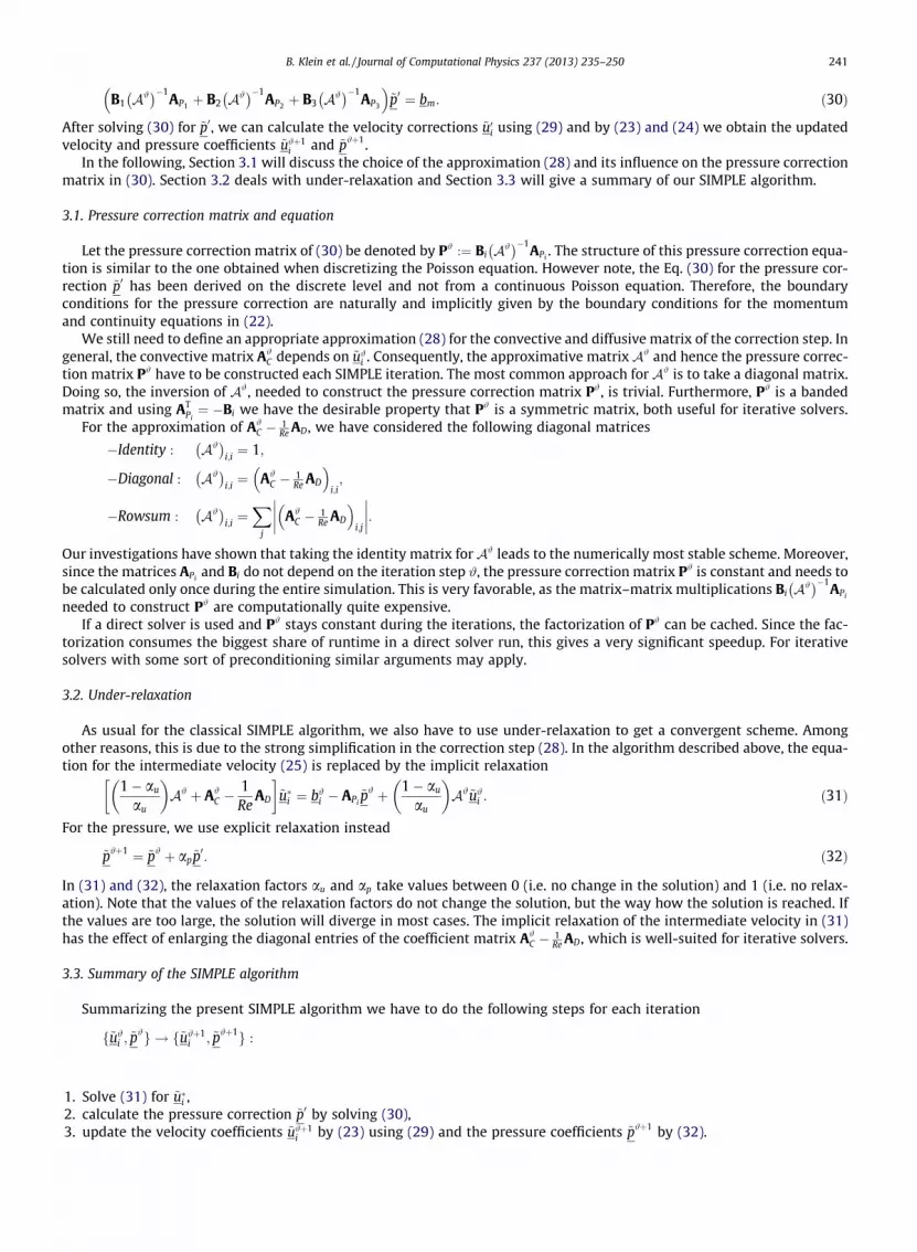
3.1. Pressure correction matrix and equation

Let the pressure correction matrix of (30) be denoted by P# :¼ Bi A#� ��1

APi. The structure of this pressure correction equa-

tion is similar to the one obtained when discretizing the Poisson equation. However note, the Eq. (30) for the pressure cor-rection ~p0 has been derived on the discrete level and not from a continuous Poisson equation. Therefore, the boundaryconditions for the pressure correction are naturally and implicitly given by the boundary conditions for the momentumand continuity equations in (22).

We still need to define an appropriate approximation (28) for the convective and diffusive matrix of the correction step. Ingeneral, the convective matrix A#

C depends on ~u#i . Consequently, the approximative matrix A# and hence the pressure correc-tion matrix P# have to be constructed each SIMPLE iteration. The most common approach for A# is to take a diagonal matrix.Doing so, the inversion of A#, needed to construct the pressure correction matrix P#, is trivial. Furthermore, P# is a bandedmatrix and using AT

Pi¼ �Bi we have the desirable property that P# is a symmetric matrix, both useful for iterative solvers.

For the approximation of A#C � 1

Re AD, we have considered the following diagonal matrices

�Identity : A#� �

i;i ¼ 1;

�Diagonal : A#� �

i;i ¼ A#C � 1

Re AD

� �i;i;

�Rowsum : A#� �

i;i ¼X

j

A#C � 1

Re AD

� �i;j

�� :
Our investigations have shown that taking the identity matrix for A# leads to the numerically most stable scheme. Moreover,since the matrices APi
and Bi do not depend on the iteration step #, the pressure correction matrix P# is constant and needs tobe calculated only once during the entire simulation. This is very favorable, as the matrix–matrix multiplications Bi A#

� ��1APi

needed to construct P# are computationally quite expensive.If a direct solver is used and P# stays constant during the iterations, the factorization of P# can be cached. Since the fac-

torization consumes the biggest share of runtime in a direct solver run, this gives a very significant speedup. For iterativesolvers with some sort of preconditioning similar arguments may apply.

3.2. Under-relaxation

As usual for the classical SIMPLE algorithm, we also have to use under-relaxation to get a convergent scheme. Amongother reasons, this is due to the strong simplification in the correction step (28). In the algorithm described above, the equa-tion for the intermediate velocity (25) is replaced by the implicit relaxation

1� au

au

� �A# þ A#

C �1Re

AD

� �~u�i ¼ b#i � APi

~p# þ 1� au

au

� �A#~u#i : ð31Þ

For the pressure, we use explicit relaxation instead

~p#þ1 ¼ ~p# þ ap~p0: ð32Þ

In (31) and (32), the relaxation factors au and ap take values between 0 (i.e. no change in the solution) and 1 (i.e. no relax-ation). Note that the values of the relaxation factors do not change the solution, but the way how the solution is reached. Ifthe values are too large, the solution will diverge in most cases. The implicit relaxation of the intermediate velocity in (31)has the effect of enlarging the diagonal entries of the coefficient matrix A#

C � 1Re AD, which is well-suited for iterative solvers.

3.3. Summary of the SIMPLE algorithm

Summarizing the present SIMPLE algorithm we have to do the following steps for each iteration

f~u#i ; ~p#g ! f~u#þ1

i ; ~p#þ1g :

�
1. Solve (31) for ~ui ,2. calculate the pressure correction ~p0 by solving (30),3. update the velocity coefficients ~u#þ1
i by (23) using (29) and the pressure coefficients ~p#þ1 by (32).


4. Numerical results

The described algorithm has been implemented in the in-house software library BoSSS, which is currently under devel-opment at the Chair of Fluid Dynamics, TU Darmstadt. It is programmed in C# in an object-oriented design and is MPI par-allel. Right from the outset, the code was based on the discontinuous Galerkin method and designed as a library to solvearbitrary conservation laws. Various grid types (triangles, quads, tetras, cubes) can be used in different dimensions (1D–3D).

We will show numerical results for five test cases: the Poiseuille flow, the channel flow with constant transpiration [12],the Kovasznay flow [13], the flow into a corner [12] and the backward-facing step flow [14]. For all test cases the sparse di-rect solver PARDISO [15,16] is used to solve the systems of linear equations in the SIMPLE algorithm due to relatively smallproblem sizes.

Unless otherwise stated, the initial guess for the SIMPLE iterations at # ¼ 0 is set to zero, i.e. ~u0i ¼ 0 and ~p0 ¼ 0. As men-

tioned in Section 3.1, the choice of the identity matrix for A# led to the numerically most stable scheme and considering onesingle iteration of the SIMPLE algorithm it is also the computationally cheapest option. Therefore, this approach is used for alltest cases. Regarding the equal- and mixed-order formulations, the former one is only numerically stable for some test cases.For the Poiseuille flow results for both formulations are shown and compared. The numerical solutions for the remainingcases are obtained using the mixed-order formulation. Before showing the results and the convergence of the DG methodfor the individual problems, the convergence behavior of the SIMPLE algorithm as a function of the relaxation factors au

and ap is discussed.

4.1. Convergence behavior and performance of the SIMPLE algorithm

The convergence behavior of the SIMPLE algorithm is examined for taking the identity matrix for A#. The relaxation fac-tors au and ap are varied independently from 0:1 to 1:0 by steps of 0:1. The calculations are terminated when the L2-norms ofthe pressure correction kp0hkL2ðXÞ and the change in each velocity component during one SIMPLE iteration ku#þ1

hi � u#hikL2ðXÞreach the specified tolerances, after a maximum number of iterations or in case of divergence (denoted as NaN). This con-vergence study is carried out for all test cases reported herein using the mixed-order formulation with degrees k ¼ 2 for thevelocity and k0 ¼ 1 for the pressure. The individual grid sizes, the tolerances for the pressure correction and for the change inthe velocity as well as the maximum number of iterations are given in the tables below. The initial guess for velocity andpressure is set to zero for all problems.

From the results in the Tables 1–5 it can be seen that the fastest convergence is achieved for ap ¼ 0:9 for the channel flowwith constant transpiration and for ap ¼ 1:0 for all the other test cases, which means that (almost) no under-relaxation forthe pressure is needed (at least for the problems we simulated). This is quite remarkable and to the best of our knowledge instrong contrast to the application of the SIMPLE algorithm in the context of the finite volume method or the continuous finiteelement method. For the finite volume method one usually applies the rule of thumb ap ¼ 1� au [17], where typical valuesfor au are between 0:6 and 0:8 and for ap between 0:2 and 0:4. Also [11] reports using under-relaxation for the pressure whenapplying the SIMPLE algorithm within the continuous finite element method. The optimal values for the relaxation factor ofthe velocity au differ for the different problems. For the two cases, where Dirichlet boundary conditions for the velocity areused on all boundaries, namely the Kovasznay flow and the flow into a corner, the optimal value for the relaxation factor ofthe velocity is au ¼ 1:0, which means that no under-relaxation at all is needed for these cases. Table 6 gives a summary of theoptimal values for the relaxation factors together with the computational time measured on a Intel Core i5 Quad Core(3.10 GHz) with 8.00 GB main memory. Simulations are run on a single processor except for the direct solver PARDISO, whichis OpenMP parallel.

4.2. Poiseuille flow

The first test case carried out is a simple 2D channel flow with Re ¼ 100. The computational domain X ¼ ½0;10� � ½�1;1� isdiscretized by uniform Cartesian grids. The grids are successively refined by Dxi ¼ Dx0=2i, where Dx0 ¼ 0:5 belongs to the

Table 1Number of SIMPLE iterations as a function of the relaxation factors au and ap for the Poiseuille flow using a grid with 4� 20 cells and tolerances for kp0hkL2 ðXÞ andku#þ1

hi � u#hikL2 ðXÞ of 1.0e-10. The optimal value is bold-faced.

ap = 0.1 ap = 0.2 ap = 0.3 ap = 0.4 ap = 0.5 ap = 0.6 ap = 0.7 ap = 0.8 ap = 0.9 ap = 1.0

au = 0.1 >1000 >1000 >1000 940 766 647 562 497 447 407au = 0.2 >1000 >1000 998 769 627 531 461 408 366 332au = 0.3 >1000 >1000 >1000 780 636 539 469 417 375 341au = 0.4 >1000 >1000 >1000 847 686 600 525 464 415 375au = 0.5 >1000 >1000 >1000 918 739 619 532 498 445 401au = 0.6 >1000 >1000 >1000 984 792 663 591 524 474 441au = 0.7 >1000 >1000 >1000 >1000 855 741 660 598 551 516au = 0.8 >1000 >1000 >1000 >1000 961 835 747 683 >1000 NaNau = 0.9 >1000 >1000 >1000 >1000 >1000 NaN NaN NaN NaN NaNau = 1.0 >1000 >1000 >1000 NaN NaN NaN NaN NaN NaN NaN

Table 2Number of SIMPLE iterations as a function of the relaxation factors au and ap for the channel flow with constant transpiration using a grid with 4� 20 cells andtolerances for kp0hkL2 ðXÞ and ku#þ1

hi � u#hikL2ðXÞ of 1.0e-10. The optimal value is bold-faced.


au = 0.1 >1000 >1000 >1000 924 752 635 550 486 440 443au = 0.2 >1000 >1000 972 746 607 512 444 392 351 318au = 0.3 >1000 >1000 879 675 549 464 402 355 318 288au = 0.4 >1000 >1000 821 631 514 435 377 333 299 271au = 0.5 >1000 >1000 777 599 489 414 359 318 285 259au = 0.6 >1000 >1000 738 570 467 396 345 305 274 249au = 0.7 >1000 994 697 542 445 379 330 292 261 234au = 0.8 >1000 893 637 500 413 352 304 262 209 224au = 0.9 >1000 808 548 413 339 303 286 275 270 273au = 1.0 >1000 951 661 510 417 353 307 272 NaN NaN

Table 3Number of SIMPLE iterations as a function of the relaxation factors au and ap for the Kovasznay flow using a grid with 8� 8 cells and tolerances for kp0hkL2ðXÞ andku#þ1



au = 0.1 >2500 >2500 >2500 >2500 >2500 >2500 2207 1931 1717 1545au = 0.2 >2500 >2500 >2500 >2500 >2500 2456 2105 1841 1637 1473au = 0.3 >2500 >2500 >2500 >2500 >2500 2417 2071 1811 1610 1448au = 0.4 >2500 >2500 >2500 >2500 >2500 2397 2054 1797 1596 1436au = 0.5 >2500 >2500 >2500 >2500 >2500 2385 2044 1788 1588 1429au = 0.6 >2500 >2500 >2500 >2500 >2500 2377 2037 1782 1583 1424au = 0.7 >2500 >2500 >2500 >2500 >2500 2372 2032 1777 1579 1421au = 0.8 >2500 >2500 >2500 >2500 >2500 2367 2028 1774 1576 1418au = 0.9 >2500 >2500 >2500 >2500 >2500 2364 2025 1771 1573 1415au = 1.0 >2500 >2500 >2500 >2500 >2500 2360 2022 1768 1571 1413

Table 4Number of SIMPLE iterations as a function of the relaxation factors au and ap for the flow into a corner using a grid with 6� 6 cells and tolerances for kp0hkL2ðXÞand ku#þ1



au = 0.1 >2500 >2500 >2500 1947 1558 1299 1114 975 867 780au = 0.2 >2500 >2500 >2500 1937 1550 1292 1108 969 862 776au = 0.3 >2500 >2500 >2500 1934 1547 1290 1106 968 860 774au = 0.4 >2500 >2500 >2500 1932 1546 1289 1105 967 859 774au = 0.5 >2500 >2500 >2500 1931 1545 1288 1104 966 859 773au = 0.6 >2500 >2500 >2500 1931 1545 1287 1104 966 859 773au = 0.7 >2500 >2500 >2500 1930 1544 1287 1103 966 858 773au = 0.8 >2500 >2500 >2500 1930 1544 1287 1103 965 858 773au = 0.9 >2500 >2500 >2500 1929 1544 1287 1103 965 858 772au = 1.0 >2500 >2500 >2500 1929 1544 1287 1103 965 858 772

Table 5Number of SIMPLE iterations as a function of the relaxation factors au and ap for the backward-facing step flow using a grid with 832 cells and tolerances forkp0hkL2ðXÞ and ku#þ1

hi � u#hikL2ðXÞ of 1.0e-6. The optimal value is bold-faced.


au = 0.1 >1000 910 892 886 881 877 875 873 872 871au = 0.2 >1000 >1000 723 557 465 449 449 446 442 441au = 0.3 >1000 >1000 842 644 524 445 391 356 333 317au = 0.4 >1000 >1000 907 740 616 530 470 429 396 368au = 0.5 >1000 >1000 >1000 809 688 601 535 484 446 417au = 0.6 >1000 >1000 >1000 897 753 658 594 545 504 469au = 0.7 >1000 >1000 >1000 965 826 730 654 595 549 512au = 0.8 >1000 >1000 >1000 >1000 895 784 702 NaN NaN NaNau = 0.9 >1000 >1000 >1000 >1000 NaN NaN NaN NaN NaN NaNau = 1.0 >1000 NaN NaN NaN NaN NaN NaN NaN NaN NaN


Table 6Performance of the SIMPLE algorithm for the different test cases: optimal values for the relaxation factors au and ap , degrees of freedom (DOF) for velocity andpressure, number of SIMPLE iterations and computational time.

au ap DOF (u) DOF (p) # Iterations Time [s]

Poiseuille flow 0.2 1.0 480 240 332 20.4Channel flow with constant transpiration 0.8 0.9 480 240 209 15.6Kovasznay flow 1.0 1.0 384 192 1413 38.1Flow into a corner 1.0 1.0 216 108 772 18.9Backward-facing step flow 0.3 1.0 4992 2496 317 62.3

0 0.2 0.4 0.6 0.8 110−4

10−3

10−2

10−1

100

−Log10

(Δx)

L2 erro

r u1

k=1, k′=0, slope=1.91

k=1, k′=1, slope=1.90

Fig. 1. H-convergence for the Poiseuille flow using equal- and mixed-order formulations with best linear fits in a least square sense and its slopes.


coarsest grid with 4� 20 cells. As boundary conditions we apply the analytical solution u1ð0; x2Þ ¼ 1� x22;u2ð0; x2Þ ¼ 0 at the

inlet, the no-slip condition at the walls and @u1=@x1jx1¼10 ¼ 0; @u2=@x1jx1¼10 ¼ 0; pð10; x2Þ ¼ 0 at the outlet.Simulations are performed on four different grids for equal-order k ¼ 1; k0 ¼ 1 and mixed-order formulations k ¼ 1; k0 ¼ 0.

The L2-norm of the error of the velocity u1 with respect to the analytical solution versus the grid size is shown in Fig. 1, wherethe parameter for the grid size is normalized with respect to the coarsest grid, i.e. Dx ¼ Dxi=Dx0. For both formulations, theconvergence rates for the velocity u1 are in very good agreement with the theoretical one of kþ 1. The results for the equal-order formulation are slightly more accurate than those for the mixed-order formulation. Note that DG orders of k P 2 andk0 P 1 are already able to represent the exact solution, even with only one cell for the whole domain.

4.3. Channel flow with constant transpiration

The second test case is geometrically identical with the 2D channel of Section 4.2, but with periodic boundary conditionsin x1-direction and a constant transpiration velocity U2 through the lower and upper wall with the no-slip condition in x1-direction

u1ðx1;�1Þ ¼ 0; u2ðx1;�1Þ ¼ U2; ð33Þu1ðx1;1Þ ¼ 0; u2ðx1;1Þ ¼ U2: ð34Þ

For this case the analytical solution is known [12]. Defining the quantities

Re ¼ ushm; ð35Þ

us ¼

ffiffiffiffiffiffiffiffiffiDphqL

s; ð36Þ

where Dp;2h; L and q are the pressure difference between inlet and outlet, the height, the length and the density of a non-dimensionless channel, respectively, the exact solution is

Fig. 2.cells –


u1 ¼x2 þ 1

U2� 2ð1� expðU2ðx2 þ 1ÞReÞÞ

U2ð1� expð2U2ReÞÞ ; ð37Þ

u2 ¼ U2; ð38Þp ¼ �x1 þ C; ð39Þ

where C 2 R is an arbitrary constant. As we use periodic boundary conditions, the pressure has to be decomposed in twoparts p ¼ pG þ pC , where the first part pG ¼ �x represents the pressure gradient in x1-direction and is treated as a sourcein the momentum equation (cf. fi in (1b)) and the second part pC ¼ C is calculated by the simulation. The numerical gridsare the same as in Section 4.2 with Re ¼ 10 and U2 ¼ 0:3.

The analytical solution for the streamwise velocity profile and the numerical results on a grid with 4� 20 cells for theDG orders k ¼ 1; k ¼ 2 and k ¼ 3 are shown in Fig. 2. It can be seen how the difference between the analytical solutionand the simulation is becoming smaller for higher DG orders. In Fig. 3 the p-convergence on the coarsest grid with4� 20 cells and the h-convergence for the velocity u1 are presented. The errors are calculated in the L2-norm. Forthe p-convergence the polynomial degrees k ¼ 1; . . . ; 8 are used for the velocity. According to the mixed-order formula-tion the polynomial degree k0 for the pressure is always one order lower. As expected, for the p-convergence an expo-nential rate of convergence can clearly be seen. The test of the h-convergence is performed on four different grids withpolynomial orders k ¼ 1; . . . ; 5 and k0 ¼ 0; . . . ; 4. The results show the optimal rate of convergence of kþ 1 for thevelocity.

0 1 2 3 4−1

−0.8

−0.6

−0.4

−0.2

0

0.2

0.4

0.6

0.8

1

u1

x 2

0 1 2 3 4−1

−0.8

−0.6

−0.4

−0.2

0

0.2

0.4

0.6

0.8

1

u1

x 2

0 1 2 3 4−1

−0.8

−0.6

−0.4

−0.2

0

0.2

0.4

0.6

0.8

1

u1

x 2

Profiles of velocity u1 for k ¼ 1 (top left), k ¼ 2 (top right) and k ¼ 3 (bottom) for the channel flow with constant transpiration on a grid with 4� 20circles: simulation, line: analytical solution.

0 2 4 6 8

10−8

10−6

10−4

10−2

100

DG order velocity k

L2 erro

r u1

0 0.2 0.4 0.6 0.8 1

10−10

10−8

10−6

10−4

10−2

100

−Log10

(Δx)

L2 erro

r u1

k=1slope=1.8

k=2

slope=3.0k=3

slope=3.9k=4

slope=4.9k=5

slope=5.9

Fig. 3. P-convergence (left) on a grid with 4� 20 cells and h-convergence (right) for velocity u1 for the channel flow with constant transpiration. For the h-convergence the best linear fits in a least square sense and the corresponding slopes of the L2 errors are also plotted.


4.4. Kovasznay flow

The Kovasznay flow [13], which may be considered as the flow behind a two-dimensional grid, has the analytical solution

Fig. 4.of the L

u1 ¼ 1� expðkx1Þ cosð2px2Þ; ð40Þ

u2 ¼k

2pexpðkx1Þ sinð2px2Þ; ð41Þ

p ¼ �12

expð2kx1Þ þ C; ð42Þ

where k ¼ Re2 �

ffiffiffiffiffiffiffiffiffiffiffiffiffiffiffiffiffiffiffiffiRe2

4 þ 4p2q

. We consider the computational domain X ¼ ½�0:5;1:5� � ½�0:5;1:5� discretized by uniform

Cartesian grids. The coarsest grid consists of 4� 4 cells and is successively refined as described in Section 4.2. The analytical

0 0.2 0.4 0.6 0.8 1

10−10

10−8

10−6

10−4

10−2

100

−Log10

(Δx)

L2 erro

r vel

ocity

k=1slope=1.8k=2

slope=3.0k=3

slope=3.9

k=4

slope=5.0

k=5

slope=5.9

0 0.2 0.4 0.6 0.8 110−8

10−6

10−4

10−2

100

−Log10

(Δx)

L2 erro

r pre

ssur

e

k′=0slope=1.0

k′=1

slope=2.1k′=2

slope=3.2k′=3

slope=3.9

k′=4

slope=5.2

H-convergence for velocity (left) and pressure (right) for the Kovasznay flow. The best linear fits in a least square sense and the corresponding slopes2 errors are also plotted.


solution for the velocity is taken as Dirichlet boundary condition on all domain boundaries. For the Reynolds number Re ¼ 20is chosen.

Again, simulations are carried out on four different grids. The polynomial orders are k ¼ 1; . . . ; 5 for the velocity andk0 ¼ 0; . . . ; 4 for the pressure. The errors of the calculated velocity and pressure are measured with respect to the analyticalsolution (40)–(42) in the L2-norm. In Fig. 4 the h-convergence of the velocity and the pressure is displayed. We observe theconvergence rates kþ 1 for the velocity and k0 þ 1 for the pressure, as expected.

4.5. Flow into a corner

An analytical solution of the Navier–Stokes Eqs. (1a) and (1b) is the so-called flow into a corner [12]

Fig. 5.test cas

u1 ¼ expð�x2ReÞ � 1; ð43Þu2 ¼ expð�x1ReÞ � 1; ð44Þp ¼ � expð�Reðx1 þ x2ÞÞ þ C: ð45Þ

Depending on the Reynolds number Re the solution is nearly singular (in the limit Re!1) for u1 as x2 tends to zero, for u2 asx1 tends to zero and for p as x1 and x2 tend to zero. The computational domain used is X ¼ ½0; 0:05� � ½0;0:05�. To account forthe nearly singular behavior the numerical mesh is refined towards x1 ¼ 0 and x2 ¼ 0. The coarsest grid consists of 6� 6cells. A refined grid with 24� 24 cells is shown in Fig. 5. Using the analytical solution (43) and (44), Dirichlet boundary con-ditions are taken for the velocity on all domain boundaries and the reference point for the pressure is set to zero atðx1; x2Þ ¼ ð0:05;0:05Þ. For the Reynolds number we take Re ¼ 100.

For this test case the convergence of the SIMPLE algorithm is relatively slow even when taking the optimal values for therelaxation factors au ¼ 1:0 and ap ¼ 1:0 (cf. Table 4). This is most likely due to the nearly singular behavior and hence thesteep gradients in velocity and pressure. In order to save iterations, the DG projection of the analytical solution is used asinitial guess for the SIMPLE algorithm.

Simulations are performed on four different grids for the polynomial orders k ¼ 1; . . . ; 5 and k0 ¼ 0; . . . ; 4, respectively. Aplot of the streamlines and a contour plot of the pressure on a grid with 24� 24 cells and for the polynomial orders k ¼ 5 andk0 ¼ 4 are shown in Fig. 5. Again, a study of the h-convergence of the velocity and the pressure is carried out, which is shownin Fig. 6. As for the previous test cases the convergence rates are found to be kþ 1 for the velocity and k0 þ 1 for the pressure.

4.6. Backward-facing step flow

The backward-facing step flow is widely used as a benchmark test for numerical simulations. We set up the calculationaccording to the experiment by Armaly et al. [14]. The dimensionless geometry and a part of the non-uniform Cartesian gridclose to the step is depicted in Fig. 7. The length of the channel is chosen to make sure that the flow is fully developed at theoutlet, i.e. @u1=@x1 ¼ 0 and @u2=@x1 ¼ 0. The geometry is made dimensionless with twice the height of the channel at theinlet, L ¼ 2h, and two-thirds of the maximum of the streamwise velocity u1 at the same position, U ¼ 2=3Umax. Then the

Streamlines (left) and contour plot of the pressure (right) on a grid with 24� 24 cells with polynomial orders k ¼ 5; k0 ¼ 4 for the flow into a cornere.

0 0.2 0.4 0.6 0.8 1

10−14

10−12

10−10

10−8

10−6

10−4

10−2

−Log10

(Δx)

L2 erro

r vel

ocity

k=1

k=2

k=3

k=4

k=5

slope=2.0

slope=3.0

slope=3.9

slope=5.0

slope=5.9

0 0.2 0.4 0.6 0.8 1

10−12

10−10

10−8

10−6

10−4

10−2

−Log10

(Δx)

L2 erro

r pre

ssur

e

k′=0

k′=1

k′=2

k′=3

k′=4

slope=1.2

slope=2.0

slope=3.0

slope=4.0

slope=5.0

Fig. 6. H-convergence for velocity (left) and pressure (right) for the flow into a corner test case. The best linear fits in a least square sense and thecorresponding slopes of the L2 errors are also plotted.


Reynolds number is Re ¼ 4Umaxh=ð3mÞ, where m is the kinematic viscosity. At the walls the no-slip condition is applied andthe boundary conditions at the inlet (x1 ¼ �2) and outlet (x1 ¼ 26) are

u1ð�2; x2Þ ¼ 12x2ð1� 2x2Þ; ð46Þu2ð�2; x2Þ ¼ 0; ð47Þ@u1

@x1jx1¼26 ¼ 0; ð48Þ

@u2

@x1jx1¼26 ¼ 0; ð49Þ

pð26; x2Þ ¼ 0: ð50Þ

The entire grid consists of 3328 cells and the polynomial orders are k ¼ 5 for the velocity and k0 ¼ 4 for the pressure. For theReynolds number we take Re ¼ 300. Following [14], for this Reynolds number the flow is still laminar, two-dimensional andthere is only one recirculation zone. In Fig. 8 profiles of the velocity u1 are plotted at different positions in the streamwisedirection. Like in the experiment, we also find only one zone of recirculation in our calculation. Our point of reattachment isat ðxR; yRÞ ¼ ð3:1;�0:47Þ, which agrees very well with the values reported in [14]. Figs. 9 and 10 show a contour plot of thepressure and the streamlines in the region close to the step, respectively. In the plot of the pressure the singularity at thecorner of the step can be clearly observed.

Fig. 7. Geometry (top) and close-up of the grid (bottom) for the backward-facing step flow.

−0.2 0 0.2 0.4 0.6 0.8 1 1.2 1.4 1.6−0.47

−0.4

−0.3

−0.2

−0.1

0

0.1

0.2

0.3

0.4

0.5

u1

x 2

x1=0.0

x1=1.0

x1=4.0

x1=2.0

x1=3.1

Fig. 8. Profiles of the streamwise velocity at different locations for the backward-facing step flow.

Fig. 9. Contour plot of the pressure close to the step for the backward-facing step flow.

Fig. 10. Streamlines close to the step for the backward-facing step flow.


5. Conclusions

We have shown how the SIMPLE algorithm can be extended to solve the steady incompressible Navier–Stokes equationsdiscretized by the discontinuous Galerkin method. For the spatial discretization, we mainly followed the scheme proposedby Shahbazi et al. [5], including the local Lax-Friedrichs fluxes for the non-linear term and the symmetric interior penaltymethod for the Laplace operator (see, e.g. Arnold et al. [9]).

Introducing an iterative process the SIMPLE algorithm linearizes and decouples the discretized equations. Velocity andpressure are decomposed into intermediate and correction components. The equation for the pressure correction was de-rived on the discrete level. Finally, one has to solve only linear systems of equations (at each iteration step of the SIMPLEalgorithm) for the components of the intermediate velocity and the pressure correction, which are decoupled and thereforecan be solved sequentially.


The proposed algorithm has been implemented in the in-house software library BoSSS (Kummer et al. [8]), which is basedon modal basis polynomials. While the equal-order formulation was only stable for some test cases, using the mixed-orderformulation, i.e. order k for the velocity and order k� 1 for the pressure, leads to a numerically stable scheme. For the latter,convergence rates of kþ 1 for the velocity and k for the pressure were observed for the Poiseuille flow, the channel flow withconstant transpiration, the Kovasznay flow and the flow into a corner. For the backward-facing step flow very good agree-ment with experimental results were obtained. Employing the identity matrix for the approximation in the correction step, aconvergence study of the SIMPLE algorithm has shown that for all test cases the fastest convergence is achieved without un-der-relaxation for the pressure (or a relaxation factor for the pressure very close to ap ¼ 1:0), which is to the best of ourknowledge in strong contrast to the application of the SIMPLE algorithm in the context of the finite volume method orthe continuous finite element method.

The general decreasing trend for the number of SIMPLE iterations for an increasing relaxation factor of the pressure up toap ¼ 1:0 (cf. Section 4.1) suggests that over-relaxation for the pressure might improve the convergence speed, i.e. ap > 1:0.First tests have shown that a factor of 2–3 can be gained in terms of the number of SIMPLE iterations. A systematic study ofthis behavior is under investigation. Also, using multigrid techniques to accelerate the convergence of the presented algo-rithm is a subject of ongoing work. Iterative solvers with preconditioning will also be incorporated to test the algorithmfor simulating large-scale 3D problems. A forthcoming paper extending the proposed algorithm to solve unsteady problemsusing implicit time schemes is in preparation.

Acknowledgements

B. Klein would like to acknowledge the financial support by the Center of Smart Interfaces through a seed fund projectand in addition by the German Science Foundation (DFG) through Research Grant OB 96/31-1. F. Kummer would like toacknowledge the financial support by the German Science Foundation (DFG) through the research collaboration centerSFB568 and the Graduate School Computational Engineering at the Technische Universität Darmstadt. The authors arethankful to Prof. Yongqi Wang for proofreading of this article and his valuable comments. For many fruitful discussionswe are thankful to Björn Müller and Nehzat Emamy.

References

[1] B. Cockburn, G. Kanschat, D. Schötzau, A locally conservative LDG method for the incompressible Navier–Stokes equations, Math. Comp. 74 (2005)1067–1095.

[2] B. Rivière, V. Girault, Discontinuous finite element methods for incompressible flows on subdomains with non-matching interfaces, Comput. MethodsAppl. Mech. Eng. 195 (2006) 3274–3292.

[3] V. Girault, B. Rivière, M.F. Wheeler, A splitting method using discontinuous Galerkin for the transient incompressible Navier–Stokes equations, ESAIMMath. Model. Numer. Anal. 39 (2005) 1115–1147.

[4] F. Bassi, A. Crivellini, D.A. Di Pietro, S. Rebay, An implicit high-order discontinuous Galerkin method for steady and unsteady incompressible flows,Comput. Fluids 36 (2007) 1529–1546.

[5] K. Shahbazi, P.F. Fischer, C.R. Ethier, A high-order discontinuous Galerkin method for the unsteady incompressible Navier–Stokes equations, J. Comput.Phys. 222 (2007) 391–407.

[6] E. Ferrer, R.H.J. Willden, A high order Discontinuous Galerkin Finite Element solver for the incompressible Navier–Stokes equations, Comput. Fluids 46(2011) 224–230.

[7] S.V. Patankar, D.B. Spalding, A calculation procedure for heat, mass and momentum transfer in three-dimensional parabolic flows, Int. J. Heat MassTransfer 15 (1972) 1787–1806.

[8] F. Kummer, N. Emamy, R.M.B. Teymouri, M. Oberlack, Report on the development of a generic discontinuous Galerkin framework in .NET, in: ParCFD2009, 21st International Conference on Parallel Computational Fluid Dynamics, May 18–22, 2009, Moffett Field, California, USA.

[9] D.N. Arnold, F. Brezzi, B. Cockburn, L.D. Marini, Unified analysis of discontinuous Galerkin methods for elliptic problems, SIAM J. Numer. Anal. 39(2002) 1749–1779.

[10] K. Shahbazi, An explicit expression for the penalty parameter of the interior penalty method, J. Comput. Phys. 205 (2005) 401–407.[11] V. Haroutunian, M.S. Engelman, I. Hasbani, Segregated finite element algorithms for the numerical solution of large-scale incompressible flow

problems, Int. J. Numer. Methods Fluids 17 (1993) 323–348.[12] P.G. Drazin, N. Riley, The Navier–Stokes Equations: A Classification of Flows and Exact Solutions, Number 334 in London Mathematical Society Lecture

Note Series, Cambridge University Press, 2006.[13] L.I.G. Kovasznay, Laminar flow behind a two-dimensional grid, Proc. Camb. Philos. Soc. 44 (1948) 58–62.[14] B.F. Armaly, F. Durst, J.C.F. Pereira, B. Schönung, Experimental and theoretical investigation of backward-facing step flow, J. Fluid Mech. 127 (1983)

473–496.[15] O. Schenk, K. Gärtner, Solving unsymmetric sparse systems of linear equations with PARDISO, Future Gener. Comp. Syst. 20 (2004) 475–487.[16] O. Schenk, K. Gärtner, On fast factorization pivoting methods for symmetric indefinite systems, Elec. Trans. Numer. Anal. 23 (2006) 158–179.[17] J.H. Ferziger, M. Peric, Computational Methods for Fluid Dynamics, third ed., Springer, 2002.

Documents

A SIMPLE based discontinuous Galerkin solver for steady incompressible flows