Embed Size (px)
Citation preview

Implementing a Preconditioned Iterative Linear SolverUsing Massively Parallel Graphics Processing Units
by
Amirhassan Asgari Kamiabad
A thesis submitted in conformity with the requirementsfor the degree of Master of Applied Science
Graduate Department of Electrical and Computer EngineeringUniversity of Toronto
Copyright c© 2011 by Amirhassan Asgari Kamiabad

Abstract
Implementing a Preconditioned Iterative Linear Solver Using Massively Parallel
Graphics Processing Units
Amirhassan Asgari Kamiabad
Master of Applied Science
Graduate Department of Electrical and Computer Engineering
University of Toronto
2011
The research conducted in this thesis provides a robust implementation of a precondi-
tioned iterative linear solver on programmable graphic processing units (GPUs), appro-
priately designed to be used in electric power system analysis. Solving a large, sparse
linear system is the most computationally demanding part of many widely used power
system analysis, such as power flow and transient stability. This thesis presents a de-
tailed study of iterative linear solvers with a focus on Krylov-based methods. Since the
ill-conditioned nature of power system matrices typically requires substantial precon-
ditioning to ensure robustness of Krylov-based methods, a polynomial preconditioning
technique is also studied in this thesis. Programmable GPUs currently offer the best
ratio of floating point computational throughput to price for commodity processors,
outdistancing same-generation CPUs by an order of magnitude. This has led to the
widespread adoption of GPUs within a variety of computationally demanding fields such
as electromagnetics and image processing. Implementation of the Chebyshev polynomial
preconditioner and biconjugate gradient solver on a programmable GPU are presented
and discussed in detail. Evaluation of the performance of the GPU-based preconditioner
and linear solver on a variety of sparse matrices, ranging in size from 30 x 30 to 3948 x
3948, shows significant computational savings relative to a CPU-based implementation
of the same preconditioner and commonly used direct methods.
ii

Contents
1 Introduction 1
1.1 Statement of Problem . . . . . . . . . . . . . . . . . . . . . . . . . . . . 1
1.2 Thesis Objective . . . . . . . . . . . . . . . . . . . . . . . . . . . . . . . 4
1.3 Thesis Overview . . . . . . . . . . . . . . . . . . . . . . . . . . . . . . . . 6
2 Computational Challenges in Power System Analysis 7
2.1 Power Flow . . . . . . . . . . . . . . . . . . . . . . . . . . . . . . . . . . 7
2.1.1 Fast Decoupled and Dc Power flow . . . . . . . . . . . . . . . . . 9
2.2 Transient Stability . . . . . . . . . . . . . . . . . . . . . . . . . . . . . . 11
3 Methods for Solving Systems of Linear Equations 14
3.1 Direct methods: LU Decomposition . . . . . . . . . . . . . . . . . . . . . 15
3.2 Indirect Methods . . . . . . . . . . . . . . . . . . . . . . . . . . . . . . . 21
3.2.1 Conjugate Gradient . . . . . . . . . . . . . . . . . . . . . . . . . . 22
3.3 Preconditioning Methods . . . . . . . . . . . . . . . . . . . . . . . . . . . 29
3.3.1 Diagonal Scaling . . . . . . . . . . . . . . . . . . . . . . . . . . . 30
3.3.2 ILU Preconditioning . . . . . . . . . . . . . . . . . . . . . . . . . 31
3.3.3 Polynomial Preconditioning: Chebyshev Preconditioner . . . . . . 33
4 General Purpose GPU Programming 36
4.1 Architecture of Modern NVIDIA GPUs . . . . . . . . . . . . . . . . . . . 38
iii

4.2 CUDA Programming Model [1] . . . . . . . . . . . . . . . . . . . . . . . 42
5 GPU Implementation of Preconditioned Iterative Solver 47
5.1 Sparse Matrices and Storage Schemes . . . . . . . . . . . . . . . . . . . . 47
5.1.1 Coordinate Format . . . . . . . . . . . . . . . . . . . . . . . . . . 48
5.1.2 Compressed Sparse Row Format . . . . . . . . . . . . . . . . . . . 48
5.1.3 Compressed Sparse Column Format . . . . . . . . . . . . . . . . . 49
5.2 GPU Kernels . . . . . . . . . . . . . . . . . . . . . . . . . . . . . . . . . 50
5.2.1 Vector and Matrix Scaling and Addition . . . . . . . . . . . . . . 50
5.2.2 Prefix Sum . . . . . . . . . . . . . . . . . . . . . . . . . . . . . . 50
5.2.3 Vector Inner Product and Vector Norm . . . . . . . . . . . . . . . 51
5.3 Chebyshev Preconditioner Implementation . . . . . . . . . . . . . . . . . 51
5.4 BiCG-STAB Solver Implementation . . . . . . . . . . . . . . . . . . . . . 57
6 Evaluation and Results 60
6.1 Testing Platform . . . . . . . . . . . . . . . . . . . . . . . . . . . . . . . 60
6.2 Test Cases and Test Matrices . . . . . . . . . . . . . . . . . . . . . . . . 61
6.3 Evaluation of the Chebyshev Preconditioner . . . . . . . . . . . . . . . . 61
6.4 Evaluation of the BiCG-STAB Iterative Solver . . . . . . . . . . . . . . 69
6.5 Data Transfer Between CPU and GPU . . . . . . . . . . . . . . . . . . . 71
7 Conclusions and Future Work 74
A Gauss-Jacobi and Gauss-Seidel Algorithms 76
B GPU Programming Example: Dense Vector Multiplication 79
C GPU Kernels Code 83
Bibliography 96
iv

List of Tables
6.1 Impact of the 3rd order Chebyshev Preconditioner on the Condition Num-
ber and BiCG-STAB Iteration Count . . . . . . . . . . . . . . . . . . . . 65
6.2 A Comparison of the Processing Time of the GPU-Based and CPU-Based
Chebyshev Preconditioners . . . . . . . . . . . . . . . . . . . . . . . . . . 67
6.3 A Comparison of the Processing Time of the GPU-Based Chebyshev Pre-
conditioner and CPU-Based ILU Preconditioner . . . . . . . . . . . . . . 68
6.4 A Comparison of the Number of the Non-Zero Elements of the Chebyshev
Preconditioner and the ILU Preconditioner . . . . . . . . . . . . . . . . . 69
6.5 A Comparison of the Processing Time of the GPU-Based and CPU-Based
BiCG-STAB solver . . . . . . . . . . . . . . . . . . . . . . . . . . . . . . 70
6.6 A Comparison of the Processing Time of the GPU-Based and CPU-Based
Linear Solver (Chebyshev Preconditioned BiCG-STAB solver) . . . . . . 70
6.7 Comparison of MATLAB’s Direct Linear Solver on CPU and Iterative
Linear Solver on GPU . . . . . . . . . . . . . . . . . . . . . . . . . . . . 71
6.8 Memory Transfer Time: CPU to GPU . . . . . . . . . . . . . . . . . . . 72
6.9 Memory Transfer Time: GPU to GPU . . . . . . . . . . . . . . . . . . . 73
v

List of Figures
3.1 Crout LU factorization process . . . . . . . . . . . . . . . . . . . . . . . 19
3.2 Doolittle LU factorization process . . . . . . . . . . . . . . . . . . . . . 20
4.1 Enlarging Performance Gap Between GPUs and CPUs [2] . . . . . . . . . 37
4.2 NVIDIA GTX 280 hardware architecture [2] . . . . . . . . . . . . . . . . 39
4.3 32 SPs executing single instruction on multiple data . . . . . . . . . . . . 40
4.4 Streaming Multiprocessor Overview . . . . . . . . . . . . . . . . . . . . . 41
4.5 NVIDIA’s CUDA programming model . . . . . . . . . . . . . . . . . . . 43
4.6 SP scheduling to reduce the impact of memory latency . . . . . . . . . . 45
5.1 Block diagram of the Chebyshev preconditioner implementation . . . . . 52
5.2 Conversion of the matrix row vectors from dense to sparse formats in step
6 of the algorithm . . . . . . . . . . . . . . . . . . . . . . . . . . . . . . . 55
6.1 Condition number of the preconditioned coefficient matrix versus number
iterations in Chebyshev method . . . . . . . . . . . . . . . . . . . . . . . 62
6.2 Number of BiCG-STAB iterations to solve the preconditioned system ver-
sus number iterations in Chebyshev method . . . . . . . . . . . . . . . . 63
B.1 Vector multiplication: Each element in the first vector is multiplied by its
corresponding entry in the second vector . . . . . . . . . . . . . . . . . . 79
vi

Chapter 1
Introduction
1.1 Statement of Problem
The computational demands associated with power system simulations have been steadily
increasing in recent decades. One of the primary factors leading to huge computational
demand is an increased focus on wide-area system behavior, due in large part to the
recommendations of the August 2003 blackout report [3]. On August 14, 2003, approx-
imately 63 GW of electrical load was interrupted in the midwestern and northeastern
portions of the United States and southern Ontario, Canada. The blackout was due in
large part to the result of cascading outages of transmission and generation units, failures
on the energy management system (EMS) software at several control centers, and an in-
ability to manage the stability of the system after multiple, unanticipated contingencies.
Analysis of the wide-area system behavior and taking appropriate actions at early stage
could potentially have prevented the cascading effect; however, at the time neither the
wide area measurement data was available to all control centers nor was sufficient com-
puting power dedicated to wide-area system analysis. Since 2003, many efforts have been
made to share the wide area measurement data [4]. A reliable and fast analysis of the
wide-area measurements can help prevent cascading outages in large power grids; how-
1

Chapter 1. Introduction 2
ever, the ability to run the complex analysis of this considerable amount of data online
is still an unsolved challenge [5]. For instance, deployment of advanced metering systems
such as phasor measurement units (PMU) has provided the power system control centers
with a considerable amount of real time data. Modern PMU units are able to provide
accurately measured data at 60Hz frequency with better than 1µs accuracy. However,
more efficient software algorithms and faster hardware platforms should be employed to
gain full advantage of this huge amount of data.
Over the past three decades, power industries have experienced a profound restruc-
turing [6]. Power system restructuring has added another level of complexity to the
massive interconnected power grid. The introduction of competition in restructured elec-
tricity market was intended to result in better service with cheaper cost for electricity
customers. However, additional optimization and control tasks should be performed
by independent power companies [6]. Besides, a global optimization should guarantee
that all participants will benefit in the restructured system [6]. Complex market design
and advanced reliability and stability analyses require powerful parallel hardware and
dependable mathematical algorithms.
The integration of renewable resources of energy in the power system, particularly
wind power, has increased dramatically in recent years. The current wind power gener-
ation in Ontario borders on 1200MW while the total wind power generation of Canada
reaches 3500MW [7]. In Europe, the adoption levels are in the range of 5 − 20% of the
total annual demand. In the U.S., a 20% adoption level is expected by year 2030 [8].
The uncertainty associated with wind power generation adds to the complexity of the
power system. The fluctuation in weather and climate change may cause the output of
a wind unit to change within a great range [9]. Therefore, more sophisticated algorithms
accounting for the stochastic nature of wind generation must be employed to analyze the
power system and ensure the security of the system with a large penetration of these
renewable resources.

Chapter 1. Introduction 3
Real-time or faster-than-real-time power system analyses will create greater controlla-
bility over the power network and support decision making at the time of the disturbance,
which will improve the reliability of the power grid. For example, contingency analysis
is a fundamental component of the security analysis performed by control centers. The
N − 1 security criterion is generally used in evaluation of the reliability of the system.
The N − 1 security criterion corresponds to only one possible event (i.e., contingency)
among the N components of the power system. The N − k security criteria, in which k
corresponds to the number of multiple events occurring at the same time, is rarely used
in control centers due to computational complexity and relative likelihood of occurrence.
For instance, evaluating the reliability of a system with L transmission lines using the
N − 1 security criterion requires the solution of L power flow problems. If the N − 2
security criterion is used,(L2
)power flow problems have to be solved. For N − k security
criterion, the number of required power flow problems is(Lk
). Since multiple-element
events may lead to cascading outages, rigorous evaluation of such events can enhance the
security and reliability of the power system. Since multi-element contingency analysis re-
quires many more computations than single-element contingency analysis, online analysis
of N − k security needs faster algorithms and hardware. The numerical studies, software
implementation, and parallel hardware employed in this research would be beneficial to
all of the computational problems described above. Accordingly, the fast linear solver
developed in this research will improve the online analysis capabilities for large intercon-
nected power systems and mitigate many of the challenges posed by wide-area system
analysis, restructured market algorithms and integration of renewable energy resources
in power systems.

Chapter 1. Introduction 4
1.2 Thesis Objective
The main focus of this research is to develop a fast and reliable linear solver in order
to accelerate power system analysis. To keep up with new computational challenges in
power system analysis, it is imperative that power system simulation software is capable
of taking advantage of the latest advances in computer hardware. Since 2003, the increase
of clock frequency and the productive computation in each clock cycle within a single
CPU has slowed down. The main reason is the frequency limit in single core CPUs due to
power consumption issues [2]. As a result, there has been a general trend in the computer
hardware industry from single-processor CPU architectures to architectures that can use
anywhere from two to hundreds of processors.
Programmable graphics processing units (GPUs), which in some cases have hundreds
of individual cores, have become an increasingly attractive alternative to both multi-
core CPUs and high-end supercomputing hardware in areas where high computational
throughput is needed, particularly due to their high floating point operations per second
(flops) to price ratio. Research into the utilization of GPUs for simulations in a variety
of fields, including power systems, is primarily motivated by a widening gap between the
computational throughput of same-generation and same-price GPUs and CPUs.
In power system analysis tools ranging from dc power flow to transient stability, so-
lution of the linear systems arising from the Newton-Raphson algorithm (and its deriva-
tives) is often the most computationally demanding component [10–12]. Two broad
classes of solvers have been brought to bear on this problem within the power systems
area—direct solvers (of which the standard LU decomposition is the most prevalent) and
iterative solvers. Within the class of linear system iterative solvers, techniques include
Gauss-Jacobi, Gauss-Seidel [13], and Krylov subspace methods such as the conjugate gra-
dient (CG) and generalized minimum residual (GMRES) techniques. Krylov subspace
methods have been used extensively in other disciplines where large, sparse linear sys-
tems are solved in parallel [14] and can enable power system applications to fully utilize

Chapter 1. Introduction 5
the current and next generation of parallel processors. While there has already been
considerable research within the power systems community on Krylov subspace methods
[15, 16], their widespread use in the power systems field has been limited by the highly
ill-conditioned nature of the linear systems that arise in power system simulations [17].
To combat this problem, recent research efforts have aimed at developing suitable pre-
conditioners for power system matrices in order to improve the performance of Krylov
subspace methods [18–20].
This thesis presents the first preconditioned iterative linear solver for use in power
system applications that is designed for the massively parallel hardware architecture of
modern GPUs. Several attempts have been made to utilize GPUs within the power sys-
tems field in the past few years, for both visualization [21] and simulation purposes [22].
In [22], a dc power flow solver based on the Gauss-Jacobi and Gauss-Seidel algorithms
was implemented on an NVIDIA 7800 GTX chip using OpenGL (an API designed pri-
marily for graphics rendering) to carry out the iterations on the GPU. The Gauss-Seidel
and Gauss-Jacobi algorithms are rarely used in modern power system software due to
their inability to converge in many situations (e.g., for heavily loaded systems, systems
with negative reactances, and systems with poorly placed slack buses [23]), which limits
this solver’s utility. Implementations of more general linear solvers on GPUs have been
developed [24, 25], yet these solvers either fail to account for ill-conditioned coefficient
matrices or fail to take advantage of matrix sparsity. In [26], a transient stability analysis
is performed using the CUDA and new generation of NVIDIA’s graphics processing. The
author has used the LU factorization method to solve the linear systems encountered in
transient stability analysis. The sparsity of the linear systems is ignored in that paper,
resulting in poor computation time in comparison to a standard CPU implementation.
In out implementation, we use the iterative algorithms which are more suitable to the
GPU’s architecture. In addition, the sparsity of the matrices are taken into consideration
in order to save both computational time and memory space. The organization of the

Chapter 1. Introduction 6
thesis is described in the next section.
1.3 Thesis Overview
In the second chapter, an overview of some computationally demanding power system
analyses are described and it is specifically clarified how the linear solver is used in these
algorithms. The third chapter presents an overview of various linear solvers in use. The
theoretical background of the iterative linear solver implemented in this research is cov-
ered in this chapter. The importance of the preconditioning methods for the iterative
linear solvers is also discussed in Chapter 3. Chapter 4 discusses general computing on
the GPU, with specific details given regarding NVIDIA’s CUDA computing architecture.
Chapter 5 presents the implementation details of the iterative linear solver and the poly-
nomial preconditioner on the GPU. The numerical evaluation of the preconditioner and
the linear solver on the GPU and discussion of the results are presented in Chapter 6.
Chapter 7 offers conclusions and avenues for future work related to the broader use of
GPUs for power system simulation.

Chapter 2
Computational Challenges in Power
System Analysis
In this chapter, a few examples of commonly used power system analyses are discussed.
The purpose of this study is to show how the linear solver will improve the performance
of power system analysis software. Each analysis is broken down to multiple steps and
the computational load of the linear solver step is specified and compared to the other
parts of the algorithm.
2.1 Power Flow
The power flow solver is one of the most common analysis tools used in industry for
off-line and on-line studies. The solution of the power flow problem with the Newton-
Raphson method dates back to the late 1960s [23]. The power flow problem tries to find
the system bus voltages and line flows given system loads, generator terminal conditions
and network configuration [27]. The basic power flow analysis is performed by solving
the system of non-linear equations shown in (2.1) and (2.2), known as the power flow
7

Chapter 2. Computational Challenges in Power System Analysis 8
equations.
0 = ∆Pi = P inji − Vi
Nbus∑j=1
VjYij cos(δi − δj − φij) (2.1)
0 = ∆Qi = Qinji − Vi
Nbus∑j=1
VjYij sin(δi − δj − φij) (2.2)
i = 1, ..., Nbus (2.3)
In these equations,P inji and Qinj
i are the active and reactive power injected at bus i, Vi
is the voltage magnitude at bus i and δi is the voltage phasor angles at bus i. Yij and
φij are the magnitude and phasor angle of the (ij)th element of the network admittance
matrix [27, 28]. The value Nbus is the total number of buses minus one.
The prevailing option for solving the power flow equations is the Newton-Raphson
method. The Newton-Raphson method starts with an initial guess for voltage magnitudes
and phase angles and iteratively improves the solution by driving the mismatch power,
∆Pi and ∆Qi in (2.1) and (2.2), to zero. When the power mismatch is driven to zero, the
injected power at the bus and the calculated power from the voltages and phase angles is
equal. The voltage and phase angle updates in every iteration k of the Newton-Raphson
algorithm are calculated by solving the linear system in (2.4).
J(k)1 J
(k)2
J(k)3 J
(k)4
∆δ(k)1
∆δ(k)2
...
∆δ(k)Nbus
∆V(k)
1
∆V(k)
2
...
∆V(k)Nbus
= −
∆P(k)1
∆P(k)2
...
∆P(k)Nbus
∆Q(k)1
∆Q(k)2
...
∆QkNbus
(2.4)
The Jacobian matrix in (2.4) is calculated by differentiating the power flow equations

Chapter 2. Computational Challenges in Power System Analysis 9
and has the form J(k)1 J
(k)2
J(k)3 J
(k)4
=
∂∆P∂δ
∂∆P∂V
∂∆Q∂δ
∂∆Q∂V
δ=δ(k),V=V (k)
(2.5)
δ =
[δ1 δ2 . . . δNbus
], V =
[V1 V2 . . . VNbus
](2.6)
J1 to J4 sub-matrices are the partial derivatives of the power flow equations with respect
to voltage magnitudes and phase angles. After solving the linear system in (2.4) the
voltage magnitudes and phase angles are updated as
δ(k+1)i = δ
(k)i + ∆δ
(k)i (2.7)
V(k+1)i = V
(k)i + ∆V
(k)i (2.8)
The δ(k)i and V
(k)i are the power flow solutions for bus i in the kth iteration, ∆δ
(k)i and
∆V(k)i are the updates calculated from (2.4).
The Newton-Raphson method transforms the solution of non-linear power flow equa-
tions into a sequence of linear systems. The linear solver is the most computationally
expensive part of the whole procedure [29, 30]; therefore, any speed-up in this part will
result in considerable speed-up in the whole process.
2.1.1 Fast Decoupled and Dc Power flow
Decoupled power flow equations [31] can be obtained by simplifying the Jacobian in (2.5).
By neglecting the J(k)1 and J
(k)3 sub-matrices in (2.5) [28], the power flow equations reduce
to
J(k)1 ∆δ(k) = ∆P (k) (2.9)
J(k)4 ∆V (k) = ∆Q(k) (2.10)
The decoupled power flow can be solved in much shorter time than the standard power
flow; therefore, it is often used for contingency analysis where short computation time is

Chapter 2. Computational Challenges in Power System Analysis 10
desirable. In online applications, it is used to to compute approximate power flow changes
when specific generator outage or transmission line outage occurs. Further simplification
to (2.9) can be obtained by assuming that all voltage magnitudes are close to one per
unit and voltage angles across lines are small:
V (k) ≈ 1.0 (2.11)
(δi − δj) ≈ 0 (2.12)
cos(δi − δj) ≈ 1.0 (2.13)
sin(δi − δj) ≈ (δi − δj) (2.14)
In addition, it is assumed that changes in voltage magnitude have little effect on real
power and changes in voltage angles have little effect on reactive power [32], i.e.,
∂∆P
∂V≈ 0 (2.15)
∂∆Q
∂δ≈ 0 (2.16)
With these assumptions, the J1 and J4 matrices become constant and it is not necessary
to update then in every iteration [28]. These equations are known as the Fast Decoupled
Power Flow (FDPF) equations.
J1∆δ(k) = ∆P (k) (2.17)
J4∆V (k) = ∆Q(k) (2.18)
In dc power flow, it is assumed that all voltage magnitudes are equal to one per unit,
lines resistances are negligible and shunt reactances to ground are eliminated. In addition,
all shunts to ground which arise from auto-transformers are eliminated [32]. Equation
(2.18) can be neglected and the power balance equation (2.17) can be described as a
non-iterative, linear equation set
−Bδ = P (2.19)
The B matrix can be obtained by extracting the imaginary part of the Ybus matrix when
line resistances are neglected and the slack bus row and column are dropped from the

Chapter 2. Computational Challenges in Power System Analysis 11
equations set [27]. The dc power flow is a commonly used technique to calculate an
approximate real power flow over transmission lines. Further discussions on the fast
decoupled and dc power flow are available in [27, 28, 32].
2.2 Transient Stability
Traditionally, power system transient stability analysis has been performed off-line to un-
derstand the system’s ability to withstand specific disturbances and the systems response
characteristics as the system returns to steady-state operation. If a transient stability
program is run in real-time or faster than real time, then the power system control room
operators can be provided with a detailed view of the transition between steady-state
operating conditions. This view could assist an operator in understanding the impact
of contingencies and facilitate more appropriate decisions that take into account the
dynamic behavior of the system.
For transient stability analysis, the power system is modeled by a set of differential
and algebraic equations (DAEs). These equations can be described as
x = f(x, y) (2.20)
0 = g(x, y) (2.21)
where x is a vector of generator state variables which describe the machine dynamics
and y is chosen to be one of the network’s variables, which is commonly chosen to be
the bus voltage phasors in transient stability analysis. Equation (2.20) is a set of dif-
ferential equations, used to describe the dynamic behavior of synchronous machines and
excitor systems, governors and various types of controllers installed within them [10].
A synchronous machine can be modeled with as few as two and with as many as forty
differential equations [33]. The detailed modeling of synchronous machine and a discus-
sion of the differential-algebraic equations describing these machines are available in [34].

Chapter 2. Computational Challenges in Power System Analysis 12
The algebraic part of the transient stability equations, (2.21), contains the power net-
work equations describing the relation between the currents and voltages in the network.
Equations (2.20) and (2.21) form a system of DAEs that must be solved simultaneously.
DAEs are solved over a specific time period, typically several seconds following a power
disturbance to ensure that generators will remain in synchronism and voltage stability is
maintained. The common approach to solving the DAE equations of transient stability
analysis is to discretize the differential part over several time steps and use a numeri-
cal integration method to transform them to a set of algebraic equations. The use of
integration schemes to change the differential equations to algebraic equations is known
as direct discretization [35]. A commonly used form of one-step direct discretization is
shown below
dx
dt= f(x, y) (2.22)
xn+1 = xn + h [θf(tn+1, xn+1, yn+1)− (1− θ)f(tn, xn, yn)] (2.23)
In this method, xn and yn are the solution vectors at time step tn and f(tn, xn, yn) is
the evaluation of the function f for these solution vectors at time step tn. If the solution
vectors for time step tn are known, (2.23) establishes a set of non-differential, nonlinear
equations to find the solution vectors at time step tn+1. The variable h is the time step
of the numerical integration. Small time steps will generally result in smaller errors and
more accurate solutions [35]. The variable θ defines the various types of integration
methods. The θ = 1 case will result in the Backward Euler method [36] and in case of
θ = 12
the Trapezoidal method [37] is obtained. Detailed discussion of various integration
methods is available in [27, 35]. The Trapezoidal and the Backward Euler methods are
commonly used to solve transient stability problems due to their robust performance
and simple implementation. A comparison of commonly used discretization methods in
power systems is provided in [38].

Chapter 2. Computational Challenges in Power System Analysis 13
The Backward Euler method reduces (2.20) and (2.21) to the following forms:
xn+1 = xn + hf(tn+1, xn+1, yn+1) (2.24)
0 = g(xn+1, yn+1) (2.25)
where xn+1 and yn+1 are unknown. All the nonlinear algebraic equations in (2.24) and
(2.25) can be described in a compact form:
G(xn+1, yn+1) = 0 (2.26)
The nonlinear set of equations described in (2.26) can be solved by using the Newton-
Raphson algorithm. As described earlier in this chapter, the Newton-Raphson algorithm
transforms the solution of a nonlinear set of equations into a sequence of linear system
solutions; therefore, the solution of a linear system of equations is a critical part of
transient stability analysis. This thesis tries to develop a high performance linear solver
in order to achieve speed-up in power systems analyses such as power flow and transient
stability. The next chapter will discuss commonly used algorithms for solving linear
systems and will describe the specific algorithms implemented in this research.

Chapter 3
Methods for Solving Systems of
Linear Equations
Solution of a linear system is usually the most computationally expensive step in various
power system analyses such as power flow and transient stability analysis. In general, a
linear system is described as
Ax = b (3.1)
a1,1 a1,2 a1,3 . . . a1,n
a2,1 a2,2 a2,3 . . . a2,n
......
.... . .
...
an,1 an,2 an,3 . . . an,n
x1
x2
...
xn
=
b1
b2
...
bn
(3.2)
where A is a N ×N square matrix known as the coefficient matrix, b is a N × 1 vector
known as the “right-hand-side” (RHS) vector and x is a N × 1 vector known as the
“unknown” vector. One method of solving the linear system is to explicitly calculate the
inverse of the coefficient matrix and multiply it by the RHS vector
x = A−1b (3.3)
14

Chapter 3. Methods for Solving Systems of Linear Equations 15
For large, sparse matrices, such as those encountered in power systems, calculating the
inverse of the coefficient matrix introduces unnecessary computations. In addition, stor-
ing the inverse of a sparse matrix usually requires unnecessarily large amount of memory
space; thus, various methods have been developed to solve a system of linear equations
without explicitly calculating the inverse of the linear system.
Methods of solving linear systems fall into two general categories: direct methods
and indirect methods. Each category may be appropriate for linear systems arising from
specific fields of science or specific computer platforms on which the linear system is
implemented. This chapter discusses the direct and indirect methods most commonly
used in power system analyses and discusses their benefits and shortcomings. The specific
method implemented in this research is also studied in detail in this chapter.
3.1 Direct methods: LU Decomposition
The direct methods result in the solution of the linear system in a single iteration. The-
oretically, direct methods can find the exact solution of the linear system by performing
a finite number of operations [27].
The most common direct methods for solving the linear systems are based on Gaussian
elimination. The first step in the Gaussian elimination algorithm is to find the first
unknown based on other unknowns from the first equation. Then, the first unknown
is eliminated from the remaining equation using the first equation, resulting in N − 1
equations for x2...xN unknowns.
a1,1x1+ a1,2x2+ a1,3x3+ . . . a1,NxN = b1
a(1)2,2x2+ a
(1)2,3x3+ . . . a
(1)2,NxN = b
(1)2
a(1)3,2x2+ a
(1)3,3x3+ . . . a
(1)3,NxN = b
(1)3
......
......
a(1)N,2x2+ a
(1)N,3x3+ . . . a
(1)N,NxN = b
(1)N
(3.4)

Chapter 3. Methods for Solving Systems of Linear Equations 16
The superscript (1) denotes the coefficients of the linear system after the first step
of Gaussian elimination. The next step is to eliminated the second unknown from the
N − 1 equations. This process is repeated until the last equation consist of only the last
unknown:
a1,1x1+ a1,2x2+ a1,3x3+ . . . a1,NxN = b1
a(1)2,2x2+ a
(1)2,3x3+ . . . a
(1)2,NxN = b
(1)2
a(2)3,3x3+ . . . a
(2)3,NxN = b
(2)3
...
a(N−1)N,N xN = b
(N−1)N
(3.5)
This single-unknown equation immediately gives the value of the last unknown. When
the value of the last unknown is found, it is replaced in the previous equation to find the
value of xN−1. This process is repeated until all unknown values are found.
The LU decomposition method is a common algorithm for solving linear systems
which is based on Gaussian elimination. In LU factorization, the coefficient matrix is
factorized into a lower triangular and an upper triangular matrix.
A = LU (3.6)
a1,1 a1,2 a1,3 . . . a1,N
a2,1 a2,2 a2,3 . . . a2,N
......
.... . .
...
aN,1 aN,2 aN,3 . . . aN,N
=
l1,1 0 0 . . . 0
l2,1 l2,2 0 . . . 0
......
.... . .
...
lN,1 lN,2 lN,3 . . . lN,N
u1,2 u1,2 u1,3 . . . u1,N
0 u2,2 u2,3 . . . u2,N
......
.... . .
...
0 0 0 . . . uN,N
(3.7)
Then the linear system of (3.1) becomes
LUx = b (3.8)
The vector resulting from multiplying x by U is defined as z
Ux = z (3.9)
Chapter 3. Methods for Solving Systems of Linear Equations 17
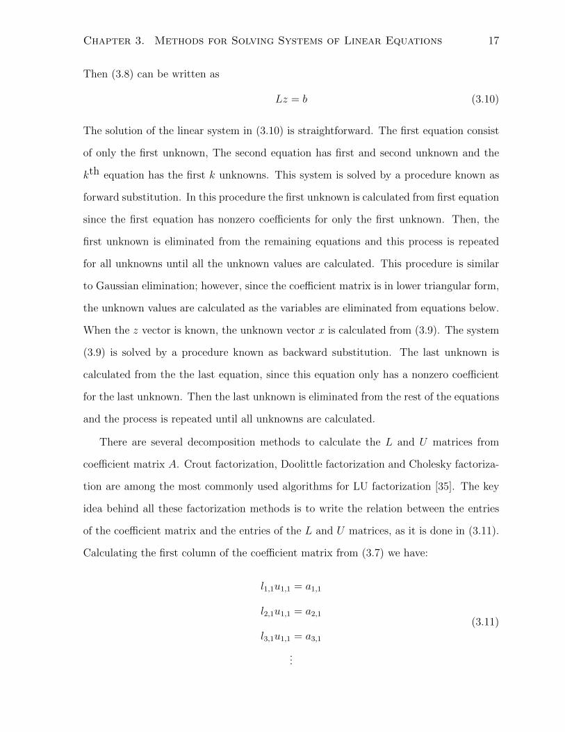
Then (3.8) can be written as
Lz = b (3.10)
The solution of the linear system in (3.10) is straightforward. The first equation consist
of only the first unknown, The second equation has first and second unknown and the
kth equation has the first k unknowns. This system is solved by a procedure known as
forward substitution. In this procedure the first unknown is calculated from first equation
since the first equation has nonzero coefficients for only the first unknown. Then, the
first unknown is eliminated from the remaining equations and this process is repeated
for all unknowns until all the unknown values are calculated. This procedure is similar
to Gaussian elimination; however, since the coefficient matrix is in lower triangular form,
the unknown values are calculated as the variables are eliminated from equations below.
When the z vector is known, the unknown vector x is calculated from (3.9). The system
(3.9) is solved by a procedure known as backward substitution. The last unknown is
calculated from the the last equation, since this equation only has a nonzero coefficient
for the last unknown. Then the last unknown is eliminated from the rest of the equations
and the process is repeated until all unknowns are calculated.
There are several decomposition methods to calculate the L and U matrices from
coefficient matrix A. Crout factorization, Doolittle factorization and Cholesky factoriza-
tion are among the most commonly used algorithms for LU factorization [35]. The key
idea behind all these factorization methods is to write the relation between the entries
of the coefficient matrix and the entries of the L and U matrices, as it is done in (3.11).
Calculating the first column of the coefficient matrix from (3.7) we have:
l1,1u1,1 = a1,1
l2,1u1,1 = a2,1
l3,1u1,1 = a3,1
...
(3.11)

Chapter 3. Methods for Solving Systems of Linear Equations 18
In the Crout factorization method, it is assumed that ui,i entries are equal to one.
Then, according to (3.11), l1,1 to lN,1 would be equal to a1,1 to aN,1 respectively and
the first column of L matrix in known. The second step is to write the first row of the
coefficient matrix based on L and U entries:
l1,1u1,2 = a1,2
l1,1u1,3 = a1,3
l1,1u1,4 = a1,4
...
(3.12)
Since l1,1 is already calculated, the first row of U matrix would be calculated from (3.12).
This process is repeated for all the columns of L matrix and row of U matrix. The Crout
method is summarized in Algorithm 1.
Algorithm 1 Crout LU factorization method
1: Load A into L and U storage locations
2: for j = 2 to N do
3: u1,i = ai,1/l1,1
4: end for
5: for k = 2 to N do
6: for i = k to N do
7: li,k = li,k −∑k−1
j=1 li,j × uj,k
8: end for
9: for i = k + 1 to N do
10: uk,i = (uk,i −∑k−1
j=1 lk,j × uj,i)/lk,k
11: end for
12: end for
The factorization order in the Crout method is shown in Figure 3.1. The odd columns
of the L matrix are calculated in odd steps and rows of U matrix are calculated in

Chapter 3. Methods for Solving Systems of Linear Equations 19
1
2
4
4
6
5factorization
Figure 3.1: Crout LU factorization process
even steps. It is important to note that entries calculated in previous steps are needed
to process the current step. Therefore parallelizing this method will face limitations
because of the serial nature of the algorithm. Figure 3.1 shows that the length of the
calculated L and U factors reduces as the process continues; therefore the computational
load of calculating the rows and columns of L and U factors reduces as the process
continues. This will usually cause unbalanced load over parallel processors and will
result in inefficient parallel implementation of the Crout method.
The Doolittle method assumes that all li,i entries are equal to one. The Doolittle
algorithm is shown in Algorithm 2. The factorization order in the Doolittle method is
shown in Figure 3.2. Note that the Doolittle method process one row of the coefficient
matrix in each step; however, the L and U entries which are calculated in each step
require the factorization results in the same step. This will lead to large amounts of
inter-core data transfer in fine grain parallel processing and the memory latency will
increase the computation time.
The Cholesky factorization is a special LU factorization technique which decomposes
the coefficient matrix into LLt. If the coefficient matrix is symmetric positive definite,
the li,i entries are real, otherwise they are complex [14]. For symmetric positive definite

Chapter 3. Methods for Solving Systems of Linear Equations 20
Algorithm 2 Doolittle LU factorization method
1: Load A into L and U storage locations
2: for k = 2 to N do
3: for i = 1 to k − 1 do
4: lk,i = (lk,i −∑k−1
j=1 lk,j × uj,i)/ui,i
5: end for
6: for i = k to N do
7: uk,i = uk,i −∑k−1
j=1 lk,j × uj,i
8: end for
9: end for
1
2
3
factorization
4
Figure 3.2: Doolittle LU factorization process
matrices, Cholesky factorization needs less computation and memory space, since only
the L matrix is calculated and saved. This Cholesky method is rarely used for power
systems analyses due to the prevalence of asymmetric, non-positive definite matrices.
The Cholesky algorithm is shown in Algorithm 3.

Chapter 3. Methods for Solving Systems of Linear Equations 21
Algorithm 3 Cholesky factorization method
1: Load A into L and Lt storage locations
2: for i = 1 to N do
3: li,i =√
(li,i −∑i−1
k=1 l2i,k)
4: for j = i+ 1 to N do
5: lj,i = (lj,i −∑i−1
k=1 li,k × lj,k)/li,i
6: end for
7: end for
3.2 Indirect Methods
The indirect (or iterative) methods start with an approximation to the solution of (3.1)
and improve this approximate solution in each iteration. The approximate solution may
converge to the exact solution in a finite or infinite number of iterations. The iterative
method can be stopped whenever the desired accuracy in the solution is obtained. In
other words, the solution is stopped when improvement in the approximate solution is
less than a pre-specified tolerance.
Two simple iterative methods, Gauss-Seidel (G-S) and Gauss-Jacobi (G-J) methods
are included in the appendix to introduce the basics of iterative methods, without deal-
ing with complex iterative algorithms. G-S and G-J are included in most undergraduate
textbooks because of their simplicity; however, their applications are limited due to the
lack of robustness [23]. Another class of widely used and efficient iterative solvers are
Krylov subspace methods. These methods are employed in various scientific fields in-
cluding power systems [15, 16]. The most commonly used Krylov based method is the
conjugate gradient (CG) method [14]. CG is an efficient algorithm for solving symmetric
positive linear systems. Moreover, CG is well-suited to parallel platforms since the math-
ematical operations used in the the CG algorithm, such as matrix-vector multiplication
and vector inner products, are efficiently implemented on parallel platforms. The CG
Chapter 3. Methods for Solving Systems of Linear Equations 22
method is guaranteed to converge only if the coefficient matrix is symmetric positive def-
inite. The other Krylov based solver discussed here is the bi-conjugate gradient (BiCG)
algorithm. The advantage of the BiCG algorithm over the CG algorithm is that BiCG
is suitable for both symmetric and nonsymmetric systems. The detailed specification of
CG and BiCG are discussed in the following subsections.
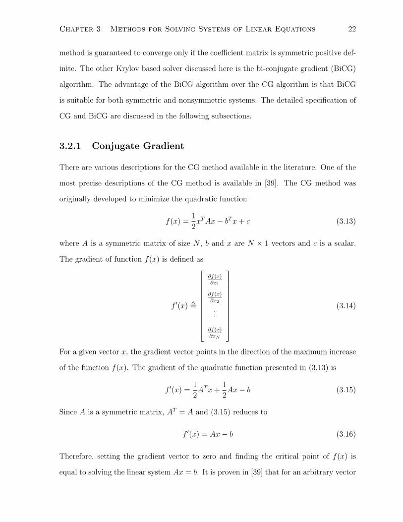
3.2.1 Conjugate Gradient
There are various descriptions for the CG method available in the literature. One of the
most precise descriptions of the CG method is available in [39]. The CG method was
originally developed to minimize the quadratic function
f(x) =1
2xTAx− bTx+ c (3.13)
where A is a symmetric matrix of size N , b and x are N × 1 vectors and c is a scalar.
The gradient of function f(x) is defined as
f ′(x) ,
∂f(x)∂x1
∂f(x)∂x2
...
∂f(x)∂xN
(3.14)
For a given vector x, the gradient vector points in the direction of the maximum increase
of the function f(x). The gradient of the quadratic function presented in (3.13) is
f ′(x) =1
2ATx+
1
2Ax− b (3.15)
Since A is a symmetric matrix, AT = A and (3.15) reduces to
f ′(x) = Ax− b (3.16)
Therefore, setting the gradient vector to zero and finding the critical point of f(x) is
equal to solving the linear system Ax = b. It is proven in [39] that for an arbitrary vector

Chapter 3. Methods for Solving Systems of Linear Equations 23
p the quadratic function can be reformed as
f(p) = f(x) +1
2(p− x)TA(p− x) (3.17)
According to the definition of the positive definite matrix, (p− x)TA(p− x) is positive if
p 6= x; therefore, If A is symmetric positive definite, the solution of linear system Ax = b
is the global minimum of the function f , (3.13). In fact, the CG method originated from
the steepest descent method, an optimization method developed to find the minimum of
the quadratic form. The steepest descent method starts at an arbitrary initial solution
x(0), and moves in the opposite direction of the gradient vector in each iteration, until it
is close enough to the solution x. As stated previously, the gradient vector f ′(x) points
in the direction of the greatest increase of f(x); therefore, moving along −f ′(x) will
decrease f most quickly. In the kth iteration, the steepest descent method will move in
−f ′(x(k)) direction.
−f ′(x(k)) = b− Ax(k) = r(k) (3.18)
The vector r(k) is called the “residual” at the kth iteration. Therefore, the steepest
descent method moves in the direction of the residual in every iteration. The steepest
descent update at the (k + 1)th iteration is
x(k+1) = x(k) + α(k)r(k) (3.19)
in which α(k) is the step size in kth iteration. In order to minimize f with respect to α,
the derivative ddαf(x(k)) is set to zero. Using the chain rule results in
d
dαf(x(k)) = f ′(x(k))T
d
dα(x(k)) = f ′(x(k))T r(k−1) = 0 (3.20)
If f ′(x(k))T r(k−1) = 0, the residual and gradient vectors are orthogonal. (3.18) shows that
f ′(x(k)) = −r(k); as a result
r(k)T r(k−1) = 0 (3.21)

Chapter 3. Methods for Solving Systems of Linear Equations 24
In order to find an explicit formula for α, the following equations are used:
r(k)T r(k−1) = 0
(b− Ax(k))T r(k−1) = 0
(b− A(x(k−1) + α(k)r(k−1)))T r(k−1) = 0
(b− Ax(k−1))T r(k−1) − α(k)(Ar(k−1))T r(k−1) = 0
(b− Ax(k−1))T r(k−1) = α(k)(Ar(k−1))T r(k−1)
r(k−1)T r(k−1) = α(k)r(k−1)T (Ar(k−1))
α(k) =r(k−1)T r(k−1)
r(k−1)TAr(k−1)(3.22)
The steepest descent method is shown in Algorithm 4.
Algorithm 4 Steepest Descent method
1: Choose an initial solution x(0), Set k=0
2: while not converged do
3: r(k) = b− Ax(k)
4: α(k) = r(k−1)T r(k−1)
r(k−1)TAr(k−1)
5: x(k+1) = x(k) + α(k)r(k)
6: Stop if ‖r(k)‖ ≤ ε, increase k
7: end while
One drawback of the steepest descent algorithm is that it usually takes steps in the
same direction as earlier steps [39]. If the steps in the same directions are combined in a
single iteration, the number of iterations decreases and the algorithm converges in fewer
iterations. This problem is solved if the update directions are forced to be orthogonal.
x(k+1) = x(k) + α(k)d(k) (3.23)
∀i, j = 1 . . . n, dTi dj = 0 (3.24)
Because orthogonality is required by (3.24), equation (3.22) cannot be used; Therefore,
the search directions are chosen to be A-orthogonal instead of orthogonal [39]. Two

Chapter 3. Methods for Solving Systems of Linear Equations 25
vectors di and dj are A-orthogonal if:
dTi Adj = 0 (3.25)
Two A-orthogonal vectors are also known as “conjugate” vectors. In order to find a
set of conjugate vectors, the Conjugate Gram-Schmidt process is used. The Conju-
gate Gram-Schmidt process starts with an arbitrary set of linearly independent vectors
u0, u1, . . . , uN−1. To construct A-orthogonal vector di, it is written as the sum of ui and
multiples of the previous conjugate directions:
d0 = u0
di = ui +i−1∑k=0
βikdk (3.26)
In order to find βik, the A-orthogonality characteristic is used:
0 = dTi Adj = uTi Auj +i−1∑k=0
βikdTi Adj
βij = −uTi AdjdTi Adj
(3.27)
Once βik is known for k = 0...i− 1; (3.26) can be solved for di.
The method of conjugate gradient combines steepest descent and the Conjugate
Gram-Schmidt method. In the CG method, the search directions are constructed by
conjugation of residuals. i.e., by setting ui = r(i). The method of conjugate gradient is
summarized in Algorithm 5.
The error vector in each iteration is defined as:
e(i) , x(k) − x (3.28)
in which x is the final solution. Then
r(k+1) = −Ae(k+1) = −A(e(k) + α(k)d(k)) = r(k) − α(k)Ad(k) (3.29)
Equation (3.29) shows that each new residual r(i−1) is a linear combination of the previous
residual ri and Ad(i−1); therefore, the new search direction in the ith iteration belongs

Chapter 3. Methods for Solving Systems of Linear Equations 26
Algorithm 5 Conjugate Gradient method
1: Choose an initial solution x(0), Set k=0
2: d(0) = r(0) = b− Ax(0)
3: repeat
4: α(k) = r(k)T r(k)
d(k)TAd(k)
5: x(k+1) = x(k) + α(k)d(k)
6: r(k+1) = r(k) − α(k)d(k)
7: β(k+1) = r(k+1)T r(k+1)
r(k)T r(k)
8: d(k+1) = r(k+1) + β(k+1)d(k)
9: k = k + 1
10: until ‖r(k+1)‖ ≤ ε
to the following subspace:
K(A, d(0)) = span{d(0), Ad(0), A2d(0), . . . , Ai−1d(0)} (3.30)
The subspace shown in (3.30) is known as a Krylov subspace [14] and the CG method and
similar methods such as BiCG-STAB [40] and GMRES [41] are called Krylov subspace
methods because they find an approximate solution to the linear system by searching the
Krylov subspace [14].
The CG method only works with symmetric positive definite systems. A way to use
conjugate gradient with non-symmetric systems is to multiply the linear system by the
transpose of the coefficient matrix.
ATAx = AT b (3.31)
Since ATA is always symmetric, the method of conjugate gradient would be suitable
again. However, the stability and the convergence rate of this method is not usually good
[14]. Therefore, other methods have been developed to solve non-symmetric systems. The
bi-conjugate gradient (BiCG) algorithm is a commonly used iterative method for solving

Chapter 3. Methods for Solving Systems of Linear Equations 27
Algorithm 6 BiCG method
1: Choose an initial solution x(0), Set k = 1
2: r(0) = b− Ax(0)
3: Choose r(0) (for example, r(0) = r(0))
4: repeat
5: z(k−1) = M−1r(k−1)
6: z(k−1) = M−1r(k−1)
7: ρ(k−1) = z(k−1)T r(k−1)
8: β(k−1) = ρ(k−1)
ρ(k−2)
9: p(k) = z(k−1) + β(k−1)p(k−1)
10: p(k) = z(k−1) + β(k−1)p(k−1)
11: q(k−1) = Ap(k)
12: q(k−1) = AT p(k)
13: α(k) = ρ(k−1)
p(k)T q(k)
14: x(k) = x(k−1) + α(k)p(k)
15: r(k) = r(k−1) − α(k)q(k)
16: r(k) = r(k−1) − α(k)q(k)
17: increase k
18: until ‖r(k)‖ ≤ ε
non-symmetric systems. The BiCG method develops two set of mutually orthogonal
sequences based on A and AT . The two sequences of residuals are:
r(i) = r(i−1) − α(i)Ap(i), r(i) = r(i−1) − α(i)AT p(i) (3.32)
and the two sequences of search directions are:
p(i) = r(i−1) + β(i−1)p(i−1), p(i) = r(i−1) + β(i−1)p(i−1) (3.33)
The BiCG algorithm is given in Algorithm 6. The BiCG method can suffer from a
slow rate of convergence. In addition, the BiCG method may fail to converge to the

Chapter 3. Methods for Solving Systems of Linear Equations 28
correct solution [42]. Due to these shortcomings, the BiCG-STAB method, a variant of
the BiCG method, is often used instead due to its improved convergence and stability
characteristics in comparison to the BiCG method [40]. The convergence analysis of
BiCG-STAB is available in [14, 40, 42]. The BiCG-STAB algorithm with preconditioner
is given in Algorithm 7.
Algorithm 7 BiCG-STAB method
1: Choose an initial solution x(0), Set k = 1
2: r(0) = b− Ax(0)
3: Choose r (for example, r = r(0))
4: repeat
5: ρk−1 = rT r(k−1)
6: β(k−1) = ρ(k−1)/ρ(k−2)
α(k−1)/ω(k−1)
7: p(k) = r(k−1) + β(k−1)(p(k−1) − ω(k−1)v(k−1))
8: p = M−1p(k)
9: v(k) = Ap
10: α(k) = ρ(k−1)
rT v(k)
11: s = r(k−1) − α(k)v(k)
12: if ‖s‖ ≤ ε1 stop and set x(k) = x(k−1) + α(k)p
13: s = M−1s
14: t = As
15: ω(k) = tT stT t
16: x(k) = x(k−1) + α(k)p+ ω(k)s
17: r(k) = s− ω(k)t
18: until ‖r(k)‖ ≤ ε2
Chapter 3. Methods for Solving Systems of Linear Equations 29
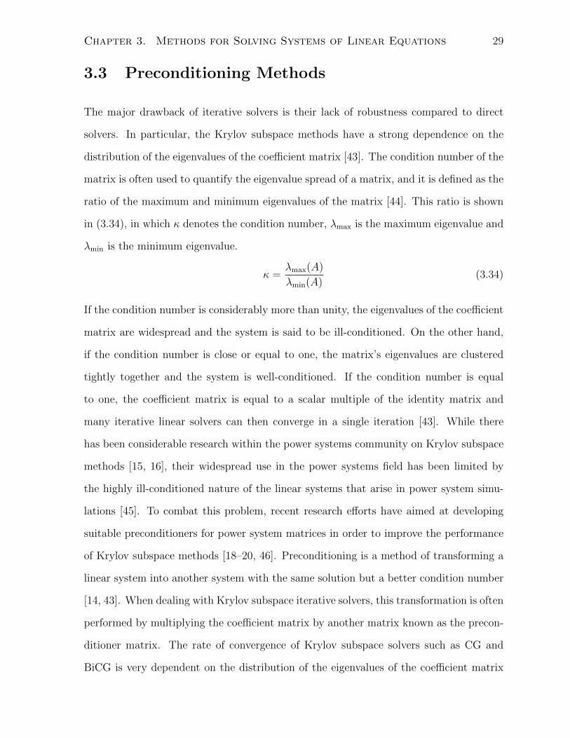
3.3 Preconditioning Methods
The major drawback of iterative solvers is their lack of robustness compared to direct
solvers. In particular, the Krylov subspace methods have a strong dependence on the
distribution of the eigenvalues of the coefficient matrix [43]. The condition number of the
matrix is often used to quantify the eigenvalue spread of a matrix, and it is defined as the
ratio of the maximum and minimum eigenvalues of the matrix [44]. This ratio is shown
in (3.34), in which κ denotes the condition number, λmax is the maximum eigenvalue and
λmin is the minimum eigenvalue.
κ =λmax(A)
λmin(A)(3.34)
If the condition number is considerably more than unity, the eigenvalues of the coefficient
matrix are widespread and the system is said to be ill-conditioned. On the other hand,
if the condition number is close or equal to one, the matrix’s eigenvalues are clustered
tightly together and the system is well-conditioned. If the condition number is equal
to one, the coefficient matrix is equal to a scalar multiple of the identity matrix and
many iterative linear solvers can then converge in a single iteration [43]. While there
has been considerable research within the power systems community on Krylov subspace
methods [15, 16], their widespread use in the power systems field has been limited by
the highly ill-conditioned nature of the linear systems that arise in power system simu-
lations [45]. To combat this problem, recent research efforts have aimed at developing
suitable preconditioners for power system matrices in order to improve the performance
of Krylov subspace methods [18–20, 46]. Preconditioning is a method of transforming a
linear system into another system with the same solution but a better condition number
[14, 43]. When dealing with Krylov subspace iterative solvers, this transformation is often
performed by multiplying the coefficient matrix by another matrix known as the precon-
ditioner matrix. The rate of convergence of Krylov subspace solvers such as CG and
BiCG is very dependent on the distribution of the eigenvalues of the coefficient matrix

Chapter 3. Methods for Solving Systems of Linear Equations 30
as will be shown in Chapter 6; therefore, preconditioning is critical to their success.
A commonly used class of preconditioners, known as the incomplete LU (ILU) fac-
torization, are based on Gaussian elimination. The key idea is to discard some fill-ins
which takes place during the factorization. In this way, the L and U factors are easier
to calculate since they have a fewer number of non-zero elements. ILU methods are
known to be highly efficient and flexible algorithms [14]. Another class of effective pre-
conditioning techniques are polynomial preconditioners [42]. These methods calculate a
series of matrix-valued polynomials and apply them to the coefficient matrix. Polynomial
preconditioning techniques are usually more amenable to parallel computing than ILU
preconditioning. The details of various preconditioning techniques are discussed in this
section.
3.3.1 Diagonal Scaling
The simplest method of preconditioning is diagonal scaling of the coefficient matrix. The
preconditioner matrix corresponding to diagonal scaling is:
M =
a−11,1 0 0 . . . 0
0 a−12,2 0 . . . 0
0 0 a−13,3 . . . 0
... 0 0. . .
...
0 0 0 . . . a−1N,N
(3.35)
Since the scaling process needs only one multiplication by a diagonal matrix, it does not
add a significant increase in computation; however, it can increase the clustering of the
eigenvalues of the coefficient matrix [44]. This effect is studied in the evaluation chapter.

Chapter 3. Methods for Solving Systems of Linear Equations 31
3.3.2 ILU Preconditioning
The L and U factors of the coefficient matrix are generally less sparse than the original
matrix [43]. Pivoting algorithms have been developed to preserve the sparsity pattern of
the original matrix after LU factorization and reduce the number of fill-ins [47], yet large
linear systems often have L and U factors with many more non-zeros than the original
matrix [35]. If any non-zero entries in the L and U factors outside the sparsity pattern
of the coefficient matrix are discarded, an incomplete L and U factors will be obtained:
M = LU (3.36)
The L and U factors in (3.36) cannot be used to solve the linear system directly; however,
they form a powerful preconditioner for iterative linear solvers. The sparsity pattern of
the a matrix A is defined as
PA = {(i, j)|a(i,j) 6= 0} (3.37)
in which a(i,j) is the (i, j)th element of matrix A. If all the fill-ins in the L and U factors
are discarded, the ILU(0) algorithm is obtained. A detailed description of this algorithm
is provided as Algorithm 8.
Algorithm 8 ILU(0)
1: for i = 2 to N do
2: for k = 1 to i− 1 and (i, k) ∈ PA do
3: Compute a(i,k) =a(i,k)a(k,k)
4: for j = k + 1 to n and (i, j) ∈ PA do
5: Compute a(i,j) = a(i,j) − a(i,k)a(k,j)
6: end for
7: end for
8: end for
In order to improve the efficiency of the ILU preconditioner, special schemes for

Chapter 3. Methods for Solving Systems of Linear Equations 32
discarding the fill-ins has been developed [14]. Fill-ins are discarded based on different
criteria, such as position, value, or a combination of the two [43].
One choice is to discard the fill-ins based on a concept known as fill-in level. The
initial level of fill of the (i, j)th element of matrix A is defined as:
levi,j =
0, if a(i,j) 6= 0 or i = j
∞, otherwise(3.38)
Each time an element is modified in line 5 of Algorithm 8, its level of fill is updated
according to:
levi,j = min{levi,j, levi,k + levk,j + 1} (3.39)
Based on this definition, an improved version of ILU, known as ILU(p) is developed. In
ILU(p), all fill-in elements whose level of fill does not exceed p are kept in the final L and
U factors. The algorithm for ILU(p) is described in Algorithm 9, in which a(i,∗) denotes
the ith row of the matrix.
Algorithm 9 ILU(p)
1: set initial values of levi,j
2: for i = 2 to N do
3: for k = 1 to i− 1 and levi,k ≤ p do
4: Compute a(i,k) =a(i,k)a(k,k)
5: Compute a(i,∗) = a(i,∗) − a(i,k)a(k,∗)
6: Update the levels of fill of the nonzero elements a(i,∗)
7: end for
8: Replace any element in row i with levij > p by zero
9: end for
Another choice of discarding the fill-ins is a threshold strategy. The threshold strategy
defines a set of rules to drop small fill-ins. A positive number τ is chosen as the drop
tolerance and fill-ins are accepted only if greater than τ in absolute value [43]. The

Chapter 3. Methods for Solving Systems of Linear Equations 33
optimal value of the drop tolerance is problem dependant and is usually chosen by a
trial-and-error approach. The threshold strategy is unable to predict the number of non-
zeros in final L and U factors. Therefore, the amount of storage needed to save the
incomplete factors is not known beforehand. Also, a threshold strategy may perform
poorly if the matrix is badly scaled (i.e., the magnitudes of the matrix entries vary over
a large range) [14]. More sophisticated preconditioning techniques can be obtained by
combining the threshold strategy, fill-in levels and scaling techniques [14, 43].
3.3.3 Polynomial Preconditioning: Chebyshev Preconditioner
The key idea of polynomial preconditioning is the approximation of the inverse of the
coefficient matrix using a matrix polynomial. The simplest polynomial preconditioner is
based on the inverse approximation using the Neumann Series [48].
A−1 =∞∑k=1
Nk (3.40)
N is a matrix with same size as matrix A. The Neumann series (3.40) results in an exact
representation of the matrix A, if A = I −N and the spectral radius of the matrix N is
less than one [42]. The corresponding preconditioner matrix can be obtained by adding
only a finite number of terms from (3.40):
Mr =r∑
k=1
Nk (3.41)
in which r is the number of polynomial terms used to calculate the preconditioner.
The Chebyshev algorithm is an iterative method originally developed for approximat-
ing the inverse of a scalar number [45]. Studies performed in [45] have shown that the
matrix-valued Chebyshev method can be used as an alternative preconditioning tech-
nique. In this method, Chebyshev polynomials are recursively calculated with the coef-
ficient matrix of the linear system taken as the argument. As the number of iterations is
increased, the linear combination of Chebyshev polynomials converges to the inverse of
the coefficient matrix [45].

Chapter 3. Methods for Solving Systems of Linear Equations 34
The first step in Chebyshev preconditioning process is the creation of Z (3.42) which
shifts the eigenvalues of the diagonally-scaled A matrix into the range [−1, 1], provided
that α and β are the minimum and maximum eigenvalues of the scaled A matrix.
Z =2
β − αAD−1 − I (3.42)
As described in [45] and [49], an estimate of β can be determined via the power method
[14], and α is assigned based on typical performance of the Chebyshev preconditioner.
Reference [45] recommends setting α = β5
if r < 3 and α = β(b r
2c×5)
if r ≥ 3, where bxc
is a function that returns the largest integer less than x. If the coefficient matrix has
known spectral characteristics, then the power method calculation can be omitted and
an approximate β can be used instead [45]. The Chebyshev polynomials are calculated
according to the following equations
T0 = I, T1 = Z (3.43)
Tk = 2ZTk−1 − Tk−2 (3.44)
M0 = c0I (3.45)
Mk = Mk−1 + ckTk (3.46)
in which Tk denotes the kth Chebyshev polynomial. The initial value for M is given
in (3.45), leading to the recursive definition of the Chebyshev preconditioner matrix
(3.46). The preconditioner matrix, M , is a linear combination of Chebyshev polynomials
calculated in (3.43) and (3.44). The coefficients of this linear combination are calculated
below:
ck =1√αβ
(−q)k (3.47)
q =1−
√αβ
1 +√
αβ
(3.48)
If r Chebyshev polynomials are used to calculate the Chebyshev preconditioner, the
resulting preconditioner matrix, Mr, can be described as in (3.49). The preconditioner

Chapter 3. Methods for Solving Systems of Linear Equations 35
matrix calculated in this way is an approximation of the inverse of the coefficient matrix.
Mr =c0
2I +
r∑k=1
ckTk ≈ A−1 (3.49)
The scalar r used as the upper bound of the summation in (3.49) denotes the number
of Chebyshev iterations. The selection of r is described in more detail in the evaluation
chapter, including discussion of the sensitivity of the preconditioner effectiveness to r
and the computational and storage costs associated with increasing r.
In contrast to preconditioning methods based on Gaussian elimination, such as ILU,
the Chebyshev method only uses matrix-matrix and matrix-vector multiplication and
addition. Most parallel processing architectures, in particular GPUs, handle these op-
erations very efficiently [50]. The linear solver implemented in this thesis consists of
Chebyshev polynomial preconditioner and BiCG-STAB solver. A brief description of
GPU architecture and programming are given in the next chapter and the implementa-
tion of the linear solver on GPU is described in Chapter 5.

Chapter 4
General Purpose GPU Programming
Since 2003, the increase of clock frequency and the productive computation in each clock
cycle within a single CPU have slowed down. The “power wall”, which refers to a limit
on clock frequencies due to an inability to handle the increase in leakage heat, is the
primary reason for the stall in processor clock speeds and represents a practical limit on
serial computation [2]. In order to increase computational throughput despite an inability
to increase clock speeds, chip manufacturers have focused on bundling several processors
together into one chip. In some cases, the number of cores put onto a single chip has been
quite modest (e.g., the Intel Core2 Duo has only two processors on-chip), yet in other
cases, most prominently in modern graphics processing units (GPUs), the trend has been
towards an ever-increasing number of cores. By putting hundreds of processors within a
single chip, GPU manufacturers (in particular, NVIDIA and AMD/ATI) have managed to
move beyond the “power wall” and reach computational speeds that are well beyond those
of same-generation CPUs. The latest GPUs are capable of processing over 1 teraflops
(i.e., 1 trillion floating point operations per second) on chips costing less than $500,
whereas a similarly priced two- or four-core CPU has peak computational throughput of
approximately 80 Gflops. Research into the utilization of GPUs for simulation in a variety
of fields, including power systems, has been driven largely by the large, steadily increasing
36

Chapter 4. General Purpose GPU Programming 37
Figure 4.1: Enlarging Performance Gap Between GPUs and CPUs [2]
gap between the peak computational throughput of CPUs and GPUs. Figure 4.1 shows
the enlarging performance gap between GPU and CPU in recent years [2]. The gap
between the computational throughput of CPU and GPU is mainly due to different design
philosophies of the two types of processors. CPUs are designed and optimized to deliver
their peak performance for sequential codes. In the CPU architectures, considerable
chip area is dedicated to large cache memories [2] to reduce the latency of the repeated
data and instruction access in complex applications. GPUs, on the other hand, are
designed to use massive number of parallel cores to perform a large amount of floating
point operations per video frame in advanced graphical applications such as video games.
Therefore, most of the chip area is reserved for hundreds of parallel cores to get peak
performance in numeric computations.
In order to develop an optimized software on either the CPU or GPU architecture,
programmers should be aware of the underlying design philosophies of each platform. An
algorithm can and often should be adapted to the CPU or GPU architecture in consid-
erably different ways to produce the best result. Since the CPU architecture has been

Chapter 4. General Purpose GPU Programming 38
available for a much longer time than the GPU architecture, programmers are more ac-
customed to CPU architectures and more sophisticated development environments and
compilers are available. As a result, a large portion of scientific software still uses se-
quential algorithms. As multicore CPUs has become more prevalent, programmers have
had to adapt sequential algorithms to new parallel platforms in order to improve per-
formance; however, the number of parallel cores in multicore CPUs is usually limited to
2 to 16 CPU cores. Therefore, the sequential algorithms divided among computational
cores and each core followed the same sequential algorithm used with earlier single core
CPUs. Special relaxation methods have been developed to divide sequential algorithms
onto multiple CPUs [51, 52]. Since the introduction of computational GPU architectures,
programmers could access hundreds of parallel cores which can communicate with low
latency. Because compilers only perform rudimentary optimization (although this is an
active area of research [53, 54]), deep understanding of the GPU architecture is needed.
In this chapter, the computational architecture of NVIDIA’s latest programmable GPUs
is described.
4.1 Architecture of Modern NVIDIA GPUs
Figure 4.2 shows the architecture of the NVIDIA GTX 280 processor used in this research.
This GPU include 240 individual processors, referred to as streaming processors (SP).
SPs are organized into 30 streaming multiprocessors (SMs). Each SM consists of a cluster
of 8 SPs which run a program in a single-instruction-multiple-data (SIMD) architecture,
which means that each SP within a given SM is always running the same instruction, but
the data that is used as the input to each instruction may (and often does) vary amongst
the individual SPs. The use of a SIMD architecture is the fundamental difference between
GPU and CPU design.
An illustrated example will be used to explain SIMD operations. Consider a group

Chapter 4. General Purpose GPU Programming 39
DRAM DRAM DRAM DRAM DRAM DRAM DRAM DRAM
SP SP SP
SP SP SP
16 KB Shared
Memory
SP
SP
SM
Global Memory
GPU
Figure 4.2: NVIDIA GTX 280 hardware architecture [2]
of 32 SPs assigned to run the following code:
if (data[i]==0) output[i]=a; else output[i]=b;
Figure 4.3 illustrates how the SIMD architecture performs. The vertical dashed lines
demonstrate the SPs’ statuses during the execution time. In the first step, the data
is loaded to all SPs. According to the SIMD structure, the SPs can perform the same
operation in parallel and if a single SP (or a set of SPs) tries to perform a different
operation, its operation will be serialized, which means all SPs will remain idle until the
diverging SP (i.e., the SPs performing a different operation) is executed. In Figure 4.3,
the statement (data[i]==0) is true only for a subset of SPs; therefore, some SPs will
remain idle while the processing of the output[i]=a statement is completed. In the next
step, output[i]=b will be executed on the remaining SPs. This example shows how the
SIMD architecture faces some limitations when algorithms include conditional branching.
Notice that during the execution of the program, a portion of SPs remain idle and the
GPU’s computational power is only partially used. In order to avoid serialized execution
on the GPU, programmers should focus more on data parallel algorithms rather than

Chapter 4. General Purpose GPU Programming 40
data[i]==0
output[i]=a output[i]=aidle idle
idle idle idleoutput[i]=b
Synchronization
Time
SP1 SP32. . .
Figure 4.3: 32 SPs executing single instruction on multiple data
task parallel algorithms. The data parallelism focuses on distributing the data across the
parallel computing cores and executing a single set of instructions on different processors.
Since all parallel cores execute the same instruction, there would be no divergence in
execution of the algorithm. In contrast, task parallelism is achieved by executing different
instructions on parallel computing cores which will cause serial execution on GPU’s SIMD
architecture.
A detailed view of a single SM is shown in Figure 4.4. Each SM in the GTX 280
is equipped with one double precision (DP) unit for double-precision operations and
two special function units (SFUs) for transcendentals. Both SPs and DP can execute
multiply-add (MAD) functions. Therefore the peak performance of GTX 280 in single

Chapter 4. General Purpose GPU Programming 41
SP
SP
SP
SP
SFU
SP
SP
SP
SP
SFU
DP
Shared Memory
Controller
Figure 4.4: Streaming Multiprocessor Overview
precision mode is:
peak performance of GTX 280 =
MAD function flops× number of SPs in an SM×
number of SMs on chip×maximum clock frequency (4.1)
however the peak performance in double precision is considerably lower since there is only
1 DP unit in an SM; therefore, on the current generation of NVIDIA’s GPUS, the single
precision computations have higher performance than double precision computations.
NVIDIA’s GTX 280 GPU has several types of memory [2]. Each SP within a SM
has access to 64KB of register space and 16KB of low-latency memory that is local to
the SM and functions similarly to the L1 cache of CPUs. SPs can also access the much
larger space of global memory (e.g. 1GB) but with a potential increase to latency. For
the GTX 280, the latency in accessing global memory is approximately 500 clock cycles
and less than 3 clock cycles for the per-SM shared memory.
In our experiments, the host (i.e., CPU) memory and GPU memory were connected
through a PCIe 16x link. The theoretical peak bandwidth of the PCIe 16x link is rated
Chapter 4. General Purpose GPU Programming 42
at 8GB/s. The global memory bandwidth of the GPU is much higher and is rated at 141
GB/s.
4.2 CUDA Programming Model [1]
Until 2006, programmers were forced to use graphics APIs such as OpenGL [55] and
DirectX [2], combined with custom fragment and vertex shaders written in proprietary
languages such as Cg and GLSL, in order to carry out general computing tasks on GPUs.
With the introduction of NVIDIA’s CUDA [1], ATI’s Stream [56], and the cross-platform
OpenCL [57] languages, programming GPUs has become increasingly similar to tradi-
tional C programming, where GPU functionality is accessed via API calls and prepro-
cessor directives. This increased ease of programming GPUs has played a large part in
elevating GPUs as one of the main parallel platforms used for high performance scientific
computing. The CUDA programming language used in this research is a set of extensions
of the C language that includes a set of compiler directives and API calls that enable
the programming of NVDIA’s CUDA-capable GPUs. The CUDA programming model
consists of host (i.e., CPU) and device (i.e., GPU) executables. A high-level view of the
CUDA programming model is illustrated in Figure 4.5. In applications where the GPU
does most of the computations, the host code is primarily used to initialize the GPU,
copy data to and from GPU memory, and initiate execution of kernels on the GPU.
In the CUDA programming model, executable code which runs on the device is known
as a “kernel”. Kernels are usually functions or algorithm designed to run in parallel on
multiple SMs of the GPU. The host side is in charge of issuing execution commands for
each kernel whereas the kernel instructions are performed on the GPU.
Kernels typically create a large number of “threads” to execute a parallel task.
Threads are the smallest units of processing that can be scheduled to run on SPs in
parallel. All threads associated with a particular kernel (e.g., Kernel 1 in Figure 4.5) are

Chapter 4. General Purpose GPU Programming 43
Block
(1,0)
Block
(2,0)
Block
(0,1)
Block
(2,1)
Block
(0,0)
Block
(1,1)
Grid 1
Block
(1,0)
Block
(2,0)
Block
(0,1)
Block
(2,1)
Block
(0,0)
Block
(1,1)
Grid N
Block
(1,2)
Block
(2,2)
Block
(0,3)
Block
(2,3)
Block
(0,2)
Block
(1,3)
Device (GPU)
Kernel 1
Kernel N
Host (CPU)
Sequential
Program
Flow
.
.
....
Thread
(1,0)
Thread
(2,0)
Thread
(0,1)
Thread
(2,1)
Thread
(0,0)
Thread
(1,1)
Thread
(3,0)
Thread
(4,0)
Thread
(4,1)
Thread
(3,1)
Block (1,3)
Figure 4.5: NVIDIA’s CUDA programming model
allocated to a thread pool, known as a “grid” in CUDA nomenclature. The grid is sub-
divided into a set of “thread blocks”, where each block has the same number of threads.
Grids can be one- or two-dimensional with a maximum of 65535 blocks in each dimen-
sion. Each block within the grid is composed of up to 512 threads. These threads can be
organized as a one-, two- or three-dimensional arrays with a maximum of 512 threads in
the 1st and 2nd dimensions and a maximum of 64 threads in the 3rd dimension. Two-
or three-dimensional blocks are typically used to simplify the memory addressing when
processing multidimensional data.
The organization of the thread blocks is a key design choice, since all thread blocks
must be able to run completely independently of one another. By enforcing strict separa-
tion in both instruction and data between the thread blocks, the GPU’s thread scheduler
has complete flexibility in dispatching threads in order to maximize the utilization of the
individual processor cores (SPs). Execution of each thread block is scheduled opportunis-
tically on available SMs on the GPU, with the guarantee that all threads within a thread

Chapter 4. General Purpose GPU Programming 44
block will execute on the same SM. In the GTX 280 GPU, when a block of threads is
assigned to a SM, the block is then divided into 32-thread units known as “warps”. A
single warp can execute on a SM at the execution time. Because threads in a given block
execute within the same SM, all threads in a given thread block have access to the same
shared, low-latency memory. In addition, all threads within a thread block are allowed
to synchronize with one another through a barrier synchronization function, which can
be used to ensure all threads within the block reach the same point in the set of kernel
instructions before continuing with execution. Efficient use of synchronization calls and
shared memory are two of the key challenges in programming GPUs, since the per-block
shared memory has a much lower access time than global memory and excessive synchro-
nization calls can result in wasted time where the SPs are waiting rather than working.
Once all the threads in all thread blocks have finished executing, the host can then copy
any results from GPU memory to host memory and begin execution of a different kernel.
GPU’s shared memory is divided into several memory banks. Accesses to a single
data element within the same bank by multiple threads in a warp will cause a bank
conflict [58]. Bank conflict will result in serialization of the multiple accesses to the
same data and increases the total memory access latency. In order to achieve maximum
performance in GPU computing, bank conflicts should be avoided as much as possible.
Further discussion of bank conflicts is provided with the description of sparse matrix
multiplication in Chapter 5.
An important technique in CUDA programming which will result in optimal global
memory access is memory coalescing. Consecutive threads within a half warp (16 threads)
can coalesce their global memory access reads and writes. If threads in a half warp access
the global memory in order, the memory access will be issued simultaneously and the
access time will be reduced considerably. This feature is helpful with implementing
algorithms that requires manipulating large matrices on the GPU and is taken into
consideration in the kernels presented in Chapter 5.

Chapter 4. General Purpose GPU Programming 45
Figure 4.6: SP scheduling to reduce the impact of memory latency
One important aspect of programming for the GPU is that full utilization of the GPU
requires the number of thread blocks to be much larger than the number of processors,
since this provides the GPU’s scheduler with greater flexibility in hiding memory access
latencies. This is significantly different from the methods used to hide latencies in CPUs,
where complex look-ahead caching is used to predict the future needs of the processor(s)
and avoid the full cost of a main memory access. Reduction of effective memory latency
on a GPU is accomplished by continually reassigning SPs stuck in a synchronization or
memory access wait state to other threads that can use the SP to perform computations.
Consider the case shown in Figure 4.6, where an SP has been executing Thread 1 and,
to continue, must retrieve some data from global memory. If the SP is left idle while
the memory access is performed (as shown in the top of Figure 4.6), then potentially
useful clock cycles are wasted. To avoid this problem, the GPU thread scheduler will
do it’s best to switch the context of the SP so that it can perform useful instructions
for a different thread (as shown in the bottom of Figure 4.6). This method of masking
memory latency assumes that the bottleneck for tasks assigned to the GPU is the number

Chapter 4. General Purpose GPU Programming 46
of computations, not the number of input-output or synchronization operations. If an
algorithm is assigned to the GPU in which memory access and synchronization wait
times are generally larger than the time spent doing computations, then eventually the
thread scheduler will run out of non-blocking threads to switch in when an SP is idle (i.e.,
there would be no Thread 2 to occupy the SP in Figure 4.6). Accordingly, developing
programs that create a large number of compute-intensive threads is a key to ensuring
that the individual processors on the GPU are fully utilized. One other reason that
switching between threads works well in hiding latencies for GPUs is that the hardware
architecture is designed such that switching between threads incurs zero overhead [1].
The brief description of the GPU architecture given in this chapter will facilitate
the understanding of the implementation of the Chebyshev preconditioner and BiCG-
STAB solver on GPU which are presented in Chapter 5. Further information on GPU
architecture is available in [2] and [1].

Chapter 5
GPU Implementation of
Preconditioned Iterative Solver
This chapter provides the implementation details of the Chebyshev preconditioner and
BiCG-STAB iterative linear solver. Power system matrices are usually stored in sparse
data structures, such as compressed sparse row (CSR) or compressed sparse column
(CSC) format in order to take advantage of sparsity. We will mention some basic details
of the sparse matrices in the following section 5.1. Section 5.2 describes the impor-
tant kernels used in the implementation of the preconditioner and solver. Section 5.3
walks through the implementation of the Chebyshev preconditioner, and section 5.4 pro-
vides implementation details for the BiCG-STAB solver and describes how the complete
Chebyshev preconditioner and BiCG-STAB solver have been implemented.
5.1 Sparse Matrices and Storage Schemes
A matrix is defined as sparse if the majority of its element are zero [35]. There is no
strict boundary on the ratio of the non-zero to zero elements in defining a sparse matrix;
however, for square matrices the number of non-zeros in a sparse matrix is usually on
the order of N (the number of rows and columns of the matrix). The location of the
47

Chapter 5. GPU Implementation of Preconditioned Iterative Solver 48
non-zero elements in a sparse matrix is known as the sparsity pattern. In order to take
advantage of the significant number of zero entries within sparse matrices, sparse storage
schemes have been developed. These storage schemes only store the non-zero elements
and their indices, resulting in considerable reduction in the memory space required to
store the matrix. Sparse storage schemes are very popular in various fields of scientific
computation such as electromagnetics, circuit simulation and molecular dynamics. In
power system analysis, large, sparse matrices appear due to the low branching factor of
power systems [27] and commercial power system matrices manipulate these matrices
using data structures that account for sparsity. Some of the widely used structures in
the literature are listed below.
5.1.1 Coordinate Format
The coordinate (COO) format is a simple and easy to create sparse format. This storage
scheme is the default format used by MATLAB to manipulate sparse matrices [59]. All
the non-zero elements are saved in a data vector and the corresponding column and row
indices are stored in separate vectors. The size of these three vectors is equal to the
number of non-zeros. Despite its easy implementation, the COO format is not the most
efficient way to store sparse matrices since similar formats are able to save sparse matrices
with a lower amount of required memory space. An example of the COO sparse matrix
format is shown below:A 0 B
0 C 0
D 0 E
⇒data [A D C B E]
row indice [0 0 1 2 2]
col indice [0 2 1 0 2]
(5.1)
5.1.2 Compressed Sparse Row Format
The compressed sparse row (CSR) is a popular sparse matrix format in various fields of
scientific computation. CSR format is more efficient than COO format since it consumes

Chapter 5. GPU Implementation of Preconditioned Iterative Solver 49
less memory space. Similar to the COO format, the non-zero elements are stored in a
data vector. The column number corresponding to each non-zero elements is also stored
in a vector usually known as “indices”. A vector of size N + 1 known as the “pointer”
(ptr) vector completes the CSR format [60]. The first element of the ptr vector is zero.
The (k + 1)th element of the vector is equal to the number of nonzero elements in the
first k rows of the sparse matrix; therefore, the last element in the vector equals the total
number of non-zeros in the sparse matrix. The number of non-zeros in row i can be
readily computed as ptr(i+ 1)− ptr(i). An example of the CSR sparse matrix format is
shown below: A 0 B
0 C 0
D 0 E
⇒data [A B C D E]
indices [0 2 1 0 2]
ptr [0 2 3 5]
(5.2)
5.1.3 Compressed Sparse Column Format
The compressed sparse column (CSC) is similar to CSR format. In CSC format the row
number corresponding to each non-zero element is stored in the indices vector. Also,
the elements of the ptr vector hold the number of non-zero elements in columns of the
sparse matrix. It is useful to note that if a sparse matrix is symmetric, the CSC and CSR
representation of the matric would be the same. An example of the CSR sparse matrix
format is shown below:A 0 B
0 C 0
D 0 E
⇒data [A D C B E]
indice [0 2 1 0 2]
ptr [0 2 3 5]
(5.3)
In this example, if the matrix is symmetric (i.e. B = D), the CSR and CSC formats
would have the same representations.

Chapter 5. GPU Implementation of Preconditioned Iterative Solver 50
5.2 GPU Kernels
In this section, the primary kernels used in the implementation of the Chebyshev pre-
conditioner and BiCG-STAB solver are explained. The kernels represented here perform
mathematical operations used in the preconditioner and solver algorithms. Some of these
parallel matrix operations are implemented similarly to the vector operations available in
the the CUBLAS library [61], a library of linear algebra functions provided by NVIDIA.
However, the most computationally expensive kernels, sparse matrix-matrix multiplica-
tion and dense to sparse conversion, are not currently available in the CUBLAS library.
The discussion of these two kernels is provided in section 5.3, along with implementation
issues related specifically to the Chebyshev preconditioner.
5.2.1 Vector and Matrix Scaling and Addition
Vector and matrix update includes scaling and addition of two or more vectors. In this
kernel, matrices are manipulated in vector forms (i.e., an N × N matrix is saved and
manipulated as N consecutive vectors). This is largely due to the memory structure of
GPUs, since the GPU memory is ultimately stored in a one dimensional array. Because
of this characteristic of GPU memory, both vectors and matrices are denoted by capital
letters during the implementation chapter. Each GPU thread takes care of updating
a single element. The kernel has data parallel characteristics and is suitable to GPU
computing.
5.2.2 Prefix Sum
The prefix sum is an operation on vectors in which each element in the output vector
is the summation of all elements in the input vector up to its index. The prefix sum
operation is shown in (5.4) and (5.5):
Operand vector A =
[a1, a2, a3, . . . aN
](5.4)

Chapter 5. GPU Implementation of Preconditioned Iterative Solver 51
Result of prefix sum =
[a1, a1 + a2, a1 + a2 + a3, . . . a1 + . . .+ aN
](5.5)
The implementation and evaluations details of this kernel is available in [62]. A highly
optimized prefix sum kernel is included in the CUDA libraries [1]. We developed our own
kernels similar to the kernels included in CUDA libraries.
5.2.3 Vector Inner Product and Vector Norm
The vector inner product (or Dot product) is an operation which takes two equal length
vectors and returns a single scaler as an output. The output of inner product is calculated
by multiplying corresponding entries in two vectors and adding up those two vectors:
A =
[a1, a2, a3, . . . aN
](5.6)
B =
[b1, b2, b3, . . . bN
](5.7)
v =N∑i=1
aibi (5.8)
The inner product kernel consists of two steps. The first step is to multiply the cor-
responding elements, which is performed similar to B. The second step is to add up
all the multiplication results, which is done with a similar to the prefix sum algorithm
[62]. The CUDA libraries include kernels for vector inner products (cublasSdot()) and
vector summation (cublasSasum()) [61]. The vector norm kernel is a simplified case of
the vector inner products kernel, where both input vectors are equal.
5.3 Chebyshev Preconditioner Implementation
The Chebyshev preconditioning algorithm is divided into multiple steps as shown in
Figure 5.1. In step 1, the host (i.e., CPU) reads the coefficient matrix A from memory
and if necessary converts it to CSR format. In step 2, A is copied from host memory
to the GPU’s global memory. As mentioned in Chapter 4, the data transfer is carried

Chapter 5. GPU Implementation of Preconditioned Iterative Solver 52
Load the coefficient matrix 1
Copy coefficient matrix to
GPU memory2
Build Z matrix, set k = 13
Multiply Tk-1 by Z4
Build the kth Chebyshev
polynomial, Tk, and update
the preconditioner 5
Copy the preconditioner
matrix to the CPU
7
Convert intermediate, dense
vectors (matrices) into sparse
vectors (matrices) and store
the sparse data in memory 6
Repeat r
times,
incrementing
k each time
Figure 5.1: Block diagram of the Chebyshev preconditioner implementation
out via PCIe 16x link in our implementation. Before sending the coefficient matrix to
the GPU, an appropriately sized location must be allocated in the GPU’s global memory
to store the input and output data. The memory allocation for the coefficient matrix is
straight-forward, since the number of the non-zero elements of the coefficient matrix is
known. However, the size of the output matrix (the preconditioner) is not known before
the execution of the code. In general, when two sparse matrices are multiplied together,
the number of the non-zero elements of the product matrix is unknown; therefore; it is
impossible to determine the exact memory space required to store the output matrices
beforehand. In our implementation, we allocate an arbitrarily large memory space (e.g
10 times larger than the memory space required to store the coefficient matrix) to be
able to store the result matrices. However, this is not a reliable solution for this problem

Chapter 5. GPU Implementation of Preconditioned Iterative Solver 53
and more efficient algorithms would be explored in future works.
In step 3, the linear transformation described in (3.42) is performed on the GPU.
The implementation of (3.42) requires scaling Z by a matrix and then subtracting values
from its diagonal entries. In steps 4 to step 6, GPU kernels perform the operations
given in (3.46) to (3.49) to iteratively build the Chebyshev preconditioner. The most
computationally expensive kernel is the matrix-matrix multiplication performed in step
4 (Z × T(k−1)). Because matrix-matrix multiplication can be decomposed into a set of
dot products, an efficient sparse vector-vector dot product kernel is needed.
XY = P (5.9)X1Y1 · · · X1YN
.... . .
...
XNY1 · · · XNYN
=
P1
...
PN
(5.10)
pi,k = XiYk =∑
v∈{1,2,...,N},xi,v 6=0,yv,k 6=0
xi,vyv,k (5.11)
Optimized matrix-vector kernels already exist for sparse matrices multiplying dense
vectors [60], but these kernels result in wasteful multiplications, additions, and memory
accesses due to the explicit calculations done on zero elements of the vector (e.g., in [60],
the summation in (5.11) is carried out without considering which entries in Yk are non-
zero). As indicated in the summation index given in (5.11), our calculation of an element
in the product matrix, pi,k, is carried out only if there is a non-zero element in row i and
column j of the multiplicands. This explicit consideration of the matrix sparsity results
in fewer multiply and add operations and fewer memory writes.
In the GPU implementation of (3.46) to (3.49), 16 threads are assigned to each thread
block, and each block is in charge of multiplying a single row of the sparse matrix X
with the corresponding sparse columns of Y (i.e., each 16-thread block is responsible
for computing one row of the product matrix, Pi). Therefore, each thread can access
the shared 16 banks in the shared memory without bank conflicts. Consecutive threads

Chapter 5. GPU Implementation of Preconditioned Iterative Solver 54
within a half warp (16 threads) can coalesce global memory reads and writes. If threads
in a half warp access the global memory in order, the memory access will be issued
simultaneously and the access time will reduce considerably. If the number of non-zero
entries in each row of the sparse matrix is larger than 16, the number of threads assigned
to multiplying each row should be increased; however, for sparse matrices encountered in
power system analysis, the maximum number of non-zero entries in each row is usually
in the range of 3 to 5 [27].
To carry out the summation in (5.10), each thread reads in the appropriate columns
of Y from global memory. This kernel is executed for all N rows in the multiplier matrix,
so there are as many as N thread blocks pending execution at any given time. For power
system matrices, where it is very common for N to be much larger than the number
of SMs in the GPU, the ratio of executable blocks to SMs is sufficient for the GPU’s
thread scheduler to mask the global memory access and synchronization latencies by
zero-overhead switching between thread blocks, as shown in Figure 4.6.
When step 4 is completed, each row of the product matrix is stored in shared memory
as a dense N -element vector, as shown at the top of Figure 5.2. Dense storage is used
within each block so that each thread within the block can write to the product row
without having to synchronize with any other threads. The standard data structures used
in power system software, single- and double-linked lists, would require synchronization
on each read and write operation in order to ensure that the linked list integrity is
maintained; this in turn would lead to an increase in the amount of per-thread idle time.
Although each row of the product matrix is stored in shared memory as a dense vector,
the row data is reduced to a sparse format before it is written to global memory. More
details on the dense to sparse vector conversion are provided below in the description of
step 6.
Upon completion of step 4, step 5 is carried out by determining the constant ck, as
given in equation (3.47), and performing the matrix updates given in (3.44) and (3.49).

Chapter 5. GPU Implementation of Preconditioned Iterative Solver 55
The input vector I arrives at step 6 in a
dense format:
I = 0 0 0 A 0 0 B C 0 0 D
An intermediate vector Ptr is then con-
structed according to the following rule:
Ptrj = 1 if Ij 6= 0, otherwise Ptrj = 0.
Ptr = 0 0 0 1 0 0 1 1 0 0 1
A prefix sum is then applied to the pointer
vector, with entries given by: PSj =∑ji=0 Ptri.
PS = 0 0 0 1 1 1 2 3 3 3 4
The sparse data structure, consisting of
a vector of values V and a vector of in-
dices into the dense vector, Ix, is then
constructed based on the following opera-
tions:
For k = 1, 2, . . . , N
If PSk − PSk−1 = 1
VPSk−1 = Ik
IxPSk−1 = k
Resulting in the final sparse representa-
tion of I as:
V = A B C D Ix = 3 6 7 10
Figure 5.2: Conversion of the matrix row vectors from dense to sparse formats in step 6
of the algorithm

Chapter 5. GPU Implementation of Preconditioned Iterative Solver 56
The kernel in step 6 then converts the dense row vector of the Chebyshev polynomial, Tk,
and preconditioner matrices, Mr, into a vector with CSR or CSC structure. The need
for this reduction is threefold: first, it reduces the number of high-cost global memory
writes that must be performed at the end of each iteration; secondly, it limits the amount
of global memory that must be allocated for storage of matrices between iterations; and
thirdly, it reduces the number of global memory reads that must be performed in step 4
in the subsequent iteration. The basic algorithm for this kernel is illustrated in Figure
5.2. An example of a dense vector that is obtained as the output of step 5 is shown at
the top of Figure 5.2. This vector has 4 non-zero elements, shown by the letters A to
D, at columns 3, 6, 7, and 10, respectively, with the convention that the first element of
the vector is indexed as 0. The first step in the conversion to a sparse vector is to create
an intermediate “pointer vector”, Ptr, based on which entries are non-zero in the input
vector. The elements of Ptr are set to 1 for any non-zero entries in the input vector I
and zero otherwise, as illustrated in Figure 5.2. The next step in the conversion is to
perform a prefix sum [50] on the pointer vector. To perform the prefix sum, a highly
optimized kernel included in the CUDA libraries [1] is used. The output of the prefix sum,
PS, is described and illustrated in Figure 5.2. Within the PS vector, every incremental
step between columns corresponds to the existence of a non-zero element in the input
vector (e.g., an increment occurs between PS2 and PS3 in the example of Figure 5.2,
indicating there is a non-zero entry in column 3 of the input vector). The final step
of the conversion is to use the entries in PS to first allocate the sparse data structure
(note that the last entry of PS contains the number of nonzero entries to be stored in
the sparse data structure) and populate it with the appropriate values. Vector V will be
used to update the data vector in sparse data structure, vector Ix will be used to update
the index vector and the last entry of PS will update the ptr vector. Simplified code for
this final operation, along with the resulting sparse vector data structure, is shown at
the bottom of Figure 5.2.

Chapter 5. GPU Implementation of Preconditioned Iterative Solver 57
Steps 4 to 6 are repeated r times and generate r Chebyshev polynomials in order to
carry out the summation in (3.49). At each iteration, the matrices are stored in the CSR
format. If the iterative solver is implemented on the GPU, this matrix can be read from
global memory within the solver kernel(s); otherwise, the preconditioner matrix can be
sent back to the host as indicated in step 7 of Figure 5.1.
5.4 BiCG-STAB Solver Implementation
Algorithm 10 shows the steps in the BiCG-STAB solver implementation. In the first
step, the host side loads the coefficient matrix A, the preconditioner M−1, the right hand
side vector b and the initial estimate of the solution x0. If A and M−1 matrices are
not in CSR format, they are converted to CSR format on the host side. In step 2, the
matrices A and M−1 and the vectors b and x0 are copied to GPU’s global memory. If the
solver code is executed immediately after the preconditioner, the A and M−1 matrices
are already available on GPU’s global memory and no extra copy is needed. If the initial
guess x0 is not provided, the solver assumes x(0) is a vector with all zero elements. In
step 3, the initial residual is calculated as r(0) = b − Ax(0). The Ax(0) multiplication is
performed by sparse matrix vector multiplication and the result is subtracted from b in
the same kernel. In step 4, the p(1) and r vectors are updated by copying r(0) into global
memory. Steps 5 through 18 are repeated until the method has converged or the number
of iterations is the size of the coefficient matrix. Step 6, 13 and 14 are performed by
using the inner product kernel. The sparse matrix vector multiplication kernel, defined
in section 5.3, is used in step 7, 8, 11 and 12. In step 10, 15 and 16, the vector update
kernel is used. In step 10, the norm of vector s is calculated and the result is sent back
to host memory. This norm is compared to a pre-specified tolerance (e.g. 10−3) and it is
decided whether to continue the execution or not. The same procedure is performed in
step 16 for vector r(i). The final solution is sent to host memory in step 19.

Chapter 5. GPU Implementation of Preconditioned Iterative Solver 58
Algorithm 10 Preconditioned biconjugate gradient implementation on GPU
1: Load coefficient matrix, preconditioner matrix, rhs vector and initial guess
2: Copy coefficient matrix, preconditioner matrix, rhs vector and initial guess to GPU
memory
3: Calculate the residual r(0) = b− Ax(0), Set i = 1
4: Set p(1) and r equal to r(0)
5: while not converged and i ≤ N do
6: Calculate ρi−1 = rri−1
7: Multiply p(i) by M and update p
8: Multiply p by A and update v(i)
9: Calculate rTv(i) and update αi
10: Update s, Calculate norm of s, stop if converged
11: Multiply s by M and update s
12: Multiply s by A and update t
13: Calculate tT s
14: Calculate tT t
15: Update x
16: Update r(i), Calculate norm of r(i), stop if converged,
17: Increment i
18: end while
19: Copy solution vector to host memory
The choice of the initial solution affects the performance of the iterative linear solver.
If the initial estimate of the solution is close to the exact solution of the linear system, the
iterative linear solver will converge in a relatively small number of iterations. In contrast,
if the initial solution is not close to the exact solution of the linear system, the iterative
linear solver may take a large number of iterations to converge. In our implementation,
it is possible to specify the initial solution vector. If the initial solution vector is not

Chapter 5. GPU Implementation of Preconditioned Iterative Solver 59
specified, the solver starts with an initial solution which has zeros for all its entries (“flat
start”). In the evaluation chapter, we always used flat start to measure the performance
of the iterative linear solver.
In our implementation of the BiCG-STAB solver, the linear solver will stop iterating
if the norm of the residual vector (‖r(i)‖ = ‖b−Ax(i)‖) becomes less than a pre-specified
value (“tolerance”). In general, for smaller tolerances, the iterative linear solver takes
more iterations to converge. It is possible to adjust this tolerance in our implementation
of the BiCG-STAB solver. The results presented in the evaluation chapter are based on
a tolerance of 10−3.
Finally, the GTX 280 GPU used in this research offers its maximum computational
power in 32-bit floating point (single precision) arithmetic operations. The support for
64-bit floating point (double precision) arithmetic is very limited in this generation of
NVIDIA GPUs and the double precision performance is considerably lower than the
single precision performance; therefore, the preconditioner and iterative linear solver
implemented in this research only support single-precision data.

Chapter 6
Evaluation and Results
The evaluation results of our GPU-based preconditioner and linear solver are studied in
this chapter. The testing platform and various test cases are described first. The GPU-
based Chebyshev preconditioner is applied to various test matrices and its efficiency
is studied in detail. The execution time of the GPU-based Chebyshev preconditioner
is compared to the sequential version implemented on a CPU. The execution time and
efficiency of the GPU-based Chebyshev preconditioner is also compared to the commonly
used ILU preconditioners. The GPU-based linear solver is also compared to a sequential
CPU version to measure the performance of the GPU versus CPU solution of sparse
linear systems. Finally, the performance of the preconditioned iterative solver on the
GPU is compared to state-of-the-art direct linear solvers on the CPU.
6.1 Testing Platform
The experiments were performed on a NVIDIA GTX 280-based graphics card. This
graphics card has 240 streaming processors running at a 602 MHz core clock speed. The
graphics processor has access to 1GB of global memory at peak bandwidth of 155.52
GB/s. The host side is a dual core Intel processor running with a core clock speed of
2.66GHz and 3MB of L2 cache. The serial code would be running on a single CPU core.
60

Chapter 6. Evaluation and Results 61
The connection between host memory and GPU memory is through a PCIe 16x link.
CUDA SDK version 2.0 [1] was used for programming the GPU.
6.2 Test Cases and Test Matrices
The GPU-based preconditioner and solver were tested with several sparse matrices to
determine if it is a viable alternative to a CPU-based solver. The first set of matrices
studied were the dc power flow matrices associated with the IEEE 30-, 57-, 118-, and
300-bus test cases [63]. To examine the performance on a practically-sized system, the
performance of the algorithm was also tested using the dc power flow matrix of a 1243-
bus European case [64]. Additional test matrices were obtained from the NIST Matrix
Market [65], including two matrices from the PSADMIT set (with N values of 494 and
685) and two matrices from the Harwell-Boeing Sparse Matrix Collection (with N values
of 1801 and 3948) since these two matrices are often used in the literature to evaluate
preconditioning algorithms [43]. The dc power flow matrices and matrices obtained from
NIST Matrix market are symmetric.
The right-hand-side vectors for IEEE test cases and the European case are extracted
from PowerWorld simulator, by calculating the net real power injection to each bus. For
the matrices selected from the Matrix Market collection, the entries of the right-hand-
side vectors are all equal to one. The initial solution vector for iterative solvers is equal
to zero.
6.3 Evaluation of the Chebyshev Preconditioner
One important parameter of the Chebyshev preconditioner is r, the number of Chebyshev
polynomials used to calculate the preconditioner matrix. This parameter determines the
number of times the inner loop of the Chebyshev preconditioner algorithm is traversed. At
one extreme, if the number of the Chebyshev iterations is taken to be a very large number

Chapter 6. Evaluation and Results 62
Diagonal scaling 1 2 3 4 5 6 7 8 9 10100
101
102
103
104
105
106
107
Number of Chebyshev iterations, r
Con
ditio
n nu
mbe
r of
pre
cond
ition
ed s
yste
m
30 bus system
57 bus system118 bus system
300 bus system
494 bus system
685 bus systemEU System
bcsstk14
Figure 6.1: Condition number of the preconditioned coefficient matrix versus number
iterations in Chebyshev method
(e.g., close to the dimensions of the coefficient matrix), the preconditioner calculations
would result in a very close approximation to the coefficient matrix inverse. A high-
r preconditioner would then bring the condition number of the coefficient matrix near
unity and provide a steep reduction in the number of iterations of the subsequent iterative
solver. Such a steep reduction in the solver iterations would come at a price—the number
of calculations that must be performed in the preconditioning step would increase, and
storage of the full, non-sparse inverse on the GPU could exhaust its memory capacity.
On the other hand, choosing a value of r that is too small can result in an ineffectual
preconditioner that provides no benefit to the iterative solver. For a given linear system,
it is possible to find the optimal value of r that minimizes the total time spent in both
the preconditioner and the iterative solver. This would require repeated solution of
the linear system, which runs contrary to the goal of accelerating the solution of these
systems. To settle upon a value of r for practical implementation of the preconditioner,

Chapter 6. Evaluation and Results 63
Diagonal scaling1 2 3 4 5 6 7 8 9 10100
101
102
103
104
Number of Chebyshev iterations, r
Num
ber
of B
iCG
−S
TA
B it
erat
ions
to s
olve
the
prec
ondi
tione
d sy
stem
30 bus system57 bus system118 bus system300 bus system494 bus system685 bus systemEU Systembcsstk14
Figure 6.2: Number of BiCG-STAB iterations to solve the preconditioned system versus
number iterations in Chebyshev method
sensitivity analyses were carried out in which changes in r were compared with the
resulting changes in the condition number of the coefficient matrix. For example, Figure
6.1 shows the trend in the condition number of the test matrices as r is increased. The first
step shows the reduction in condition number by scaling the coefficient matrix with the
inverse of its main diagonal, (3.35); this is separated from the Chebyshev preconditioner
effects because it is an extremely simple preconditioner and, as a result, serves as a
good baseline for evaluation. As shown in the figure, the diagonal scaling results in a
half-decade reduction in the condition number, and the Chebyshev iterations result in
another decade of reduction for values of r up to 3. Afterwards, the benefit of increasing
r is much less pronounced, indicating that the greatest gain of using the preconditioner
comes from the first few iterations. This effect is also shown in Figure 6.2 which gives the
number of BiCG-STAB iterations for solving the preconditioned linear system versus the
number of Chebyshev iterations for various test cases. Because this same phenomenon

Chapter 6. Evaluation and Results 64
was observed for the other matrices under study, it was concluded that the number of
Chebyshev iterations should be kept between two and four. After running the sensitivity
studies, the preconditioner was optimized for r values in this range as it seems to strike
a good balance between a reduction in the condition number, computational effort and
memory limits.
To understand the impact of increasing r on the size of the preconditioner matrix,
the Chebyshev polynomials are rewritten in terms of Z:
T0 = I, T1 = Z
T2 = 2ZT1 − T0 = 2Z2 − I
T3 = 2ZT2 − T1 = 4Z3 − 3Z
...
Tk ∝ Zk
(6.1)
therefore, in each Chebyshev iteration, the sparsity structure of Tk and the associated
preconditioner matrix are determined by the structure of Zk. The coefficient matrices
associated with power system analysis (e.g., from dc power flow analyses) have a sparsity
structure that is closely tied to the network topology of the study system. Based on
equation (3.42), Z has the same sparsity structure as the coefficient matrix. One way to
analyze the behavior of Zk, then, is to consider the effect of raising the adjacency matrix,
defined element-wise as
Adjm,n =
1 if Ym,n 6= 0
0 otherwise
(6.2)
to successive powers of k. From graph theory, it is known that taking the kth power
of the adjacency matrix introduces a non-zero entry at row m and column n if buses
m and n are reachable by traversing k or fewer edges (i.e., lm,n ≤ k, where lm,n is the
minimum path length between buses m and n). The diameter of the adjacency matrix,
Diam (Adj), is defined as the maximum value of lm,n over all possible row and column

Chapter 6. Evaluation and Results 65
combinations:
Diam (Adj) = max
m∈{1,2,...,N}×n∈{1,2,...,N}
lm,n (6.3)
Returning to (6.1), this suggests that any value of r equal to or greater than the diameter
of a given power network will result in a matrix that is fully dense. For many real-world
power systems, such as the Western North America, Northern China, and Central China
power grids, the diameter is significantly lower than the number of system buses [66];
therefore, a small value of r is needed to ensure the resulting preconditioner matrix is
kept sparse.
The effect of the Chebyshev preconditioner on each of the test matrices is provided
in Table 6.1.
Table 6.1: Impact of the 3rd order Chebyshev Preconditioner on the Condition Number
and BiCG-STAB Iteration Count
Matrix Size Cond# Cond# BiCG# BiCG#
Name (r = 0) (r = 3) (r = 0) (r = 3)
30-Bus 30 913.23 71.80 37 8.5
57-Bus 57 1.6×10³ 147.14 57nc 13
118-Bus 118 3.9×10³ 288.47 112 24
300-Bus 300 1.5×10⁵ 5732.5 300nc 59
494-Bus 494 3.9×10⁶ 32855.1 494nc 202
685-Bus 685 5.3×10⁵ 3542.51 685nc 82
EU case 1243 3.2×10⁵ 14244.3 1243nc 76
bcsstk14 1806 1.3×10¹⁰ 1.1×10⁵ 1806nc 42
bcsstk15 3948 7.9×10⁹ 8.9×10⁵ 3948nc 232
The data reported in the table are the size of the matrices (for a N ×N matrix, the
“size” of the matrix is N), the condition number (“Cond#”) and the number of itera-
tions it took to solve a system with the given coefficient matrix to a tolerance of 10−3

Chapter 6. Evaluation and Results 66
(“BiCG#”). The columns containing the condition number and iterative solver’s perfor-
mance data for the original, non-preconditioned matrix are labeled “r = 0”. The columns
labeled “r = 3” contain the performance data obtained after applying the Chebyshev pre-
conditioner with three iterations.
The most significant result shown in the table is that all of the cases with more than
300 buses resulted in non-convergence of the iterative solver (indicated by a superscript
“nc” in the corresponding table entries). Application of the Chebyshev preconditioner
with r = 3 resulted in a significant reduction in the condition number of all nine matrices
and, most importantly, was able to adjust the spectral properties sufficiently to get
convergence in the iterative solver. The bi-conjugate gradient stabilized (BiCG-STAB)
method was used to test the iterative solver performance, which was executed on the
host using the bicgstab function in MATLAB.
A sequential version of the Chebyshev preconditioner was also implemented in MAT-
LAB for comparison of parallel GPU and serial CPU implementations. The CPU code
accepts sparse matrices in CSR, CSC and sparse coordinate storage formats. The current
version of MATLAB does not support single precision sparse storage and computation
and the CPU computations are performed on double precision data. Table 6.2 presents
the process time of the GPU implementation versus the CPU implementation and the
speed-up ratio. The results indicate that the speed-up increases as the matrix size
increases, up to a maximum speed-up of 8.93x for the largest matrix tested. The rela-
tionship between matrix size and speed-up is especially important if the GPU is used as
a coprocessor for large power system matrices, since it indicates that the GPU imple-
mentation scales appropriately for the large linear systems that are likely to appear in
power systems applications.
The parallel Chebyshev preconditioner was also compared with the commonly used
ILU preconditioner. In order to compare the Chebyshev preconditioner on the GPU to
direct preconditioners on the CPU, the MATLAB implementation of sparse ILU factor-

Chapter 6. Evaluation and Results 67
Table 6.2: A Comparison of the Processing Time of the GPU-Based and CPU-Based
Chebyshev Preconditioners
Matrix Chebyshev Chebyshev Speed-Up
Name Time CPU(ms) Time GPU(ms) GPU vs CPU
30-Bus 0.27 0.47 0.57
57-Bus 0.68 1.25 0.54
118-Bus 1.55 2.30 0.67
300-Bus 7.69 6.47 1.18
494-Bus 19.7 8.06 1.83
685-Bus 44.1 13.72 3.21
EU case 124.2 21.03 5.91
bcsstk14 262.2 33.46 7.85
bcsstk15 591.1 66.18 8.93
ization was used. This method performs a LU factorization on the system; however, if
an element is encountered during the factorization that is less than a specified thresh-
old, that value is discarded [44]. By increasing this threshold, the ILU becomes less
incomplete and more like a full LU factorization. Each system was preconditioned with
both ILU and the three-iteration Chebyshev preconditioner then solved with the BiCG-
STAB solver. ILU preconditioner (executed on the CPU) and Chebyshev preconditioner
(executed on the GPU) computation times are given in Table 6.3.
For each test case, the ILU threshold was set such that the number of BiCG-STAB
iterations used to solve the ILU preconditioned system was same as the Chebyshev-
preconditioned system. For small system sizes, the GPU-based Chebyshev preconditioner
uses more calculation time than ILU. In these cases, the amount of computation is not
large enough to outweigh the overhead of the GPU execution, such as the time spent
to allocate the executable kernels on the GPU. In addition, for smaller matrices, the

Chapter 6. Evaluation and Results 68
Table 6.3: A Comparison of the Processing Time of the GPU-Based Chebyshev Precon-
ditioner and CPU-Based ILU Preconditioner
Matrix ILU Chebyshev Speed-Up
Name Time CPU(ms) Time GPU(ms) GPU vs CPU
30-Bus 0.331 0.47 0.70
57-Bus 0.383 1.25 0.31
118-Bus 0.519 2.30 0.23
300-Bus 2.64 6.47 0.41
494-Bus 8.91 8.06 1.11
685-Bus 25.17 13.72 1.83
EU case 46.18 21.03 2.20
bcsstk14 93.62 33.46 2.80
bcsstk15 552.11 66.18 8.34
computational resources of the GPU are not saturated by the preconditioner calculations.
As the number of calculations increases, any fixed setup overhead is amortized over more
calculations and there are more opportunities for latency masking; therefore, there should
be a relative increase in performance for larger matrices. Table 6.3 confirms that as the
matrix size increases, the GPU-based Chebyshev preconditioner requires less computation
time relative to the ILU preconditioner.
Besides the time spent on calculation in the preconditioning process, the number
of non-zeros of the preconditioned matrix is an important factor in evaluation of the
preconditioning technique. The sparsity of the preconditioned matrix has a great effect on
the computation time and memory requirements for the rest of the linear solver process.
As shown in Table 6.4, the iterative preconditioner results in a lower number of nonzero
entries for larger matrices when compared to a similarly-performing ILU preconditioner.

Chapter 6. Evaluation and Results 69
Table 6.4: A Comparison of the Number of the Non-Zero Elements of the Chebyshev
Preconditioner and the ILU Preconditioner
Matrix ILU Chebyshev
Name nnz drop tol. nnz nnz
30-Bus 108 6×10⁻² 178 258
57-Bus 205 5×10⁻² 321 461
118-Bus 464 4×10⁻² 844 1198
300-Bus 1121 5×10⁻⁴ 7113 2890
494-Bus 1080 4×10⁻⁴ 6635 4062
685-Bus 1967 4×10⁻³ 18956 9337
EU case 4872 1×10⁻³ 24826 13873
bcsstk14 32630 5×10⁻⁶ 301851 195654
bcsstk15 60882 3×10⁻⁶ 1105488 527666
6.4 Evaluation of the BiCG-STAB Iterative Solver
The iterative linear solver is compared with the serial, CPU implementation of the same
algorithm in MATLAB. Table 6.5 presents the process time of the GPU and CPU im-
plementation of the BiCG-STAB linear solver. Table 6.6 presents the process time of
the GPU and CPU implementation of the Chebyshev preconditioned BiCG-STAB lin-
ear solver. The speed-up is calculated based on the complete preconditioner and linear
solver. For the largest matrix tested, a 9.53x speed-up is achieved. As anticipated based
on the GPU architecture, the speed-up increases as the matrix size increases.
Direct solvers, especially LU factorization, are the predominant option in most power
system software. MATLAB uses a highly optimized LU factorization library, UMFPACK,
to solve large, sparse, linear systems [67]. In order to compare our developed algorithm
and implementation with the state-of-art direct linear solvers, the process time of the
MATLAB linear solver is given in Table 6.7. The process time of the GPU algorithm

Chapter 6. Evaluation and Results 70
Table 6.5: A Comparison of the Processing Time of the GPU-Based and CPU-Based
BiCG-STAB solver
Matrix BiCG BiCG Speed-up
Name Time CPU(ms) Time GPU(ms) GPU vs CPU
30-Bus 1.6 1.9 0.84
57-Bus 7.1 5.3 1.34
118-Bus 12.3 11.6 1.06
300-Bus 26.8 25.4 1.06
494-Bus 44.8 35.1 1.28
685-Bus 44.13 33.8 1.31
EU case 136.6 101.9 1.34
bcsstk14 345.3 193.1 1.79
bcsstk15 2553.1 263.7 9.68
Table 6.6: A Comparison of the Processing Time of the GPU-Based and CPU-Based
Linear Solver (Chebyshev Preconditioned BiCG-STAB solver)
Matrix Solver Solver Speed-up
Name Time CPU(ms) Time GPU(ms) GPU vs CPU
30-Bus 1.87 2.37 0.79
57-Bus 7.78 6.55 1.18
118-Bus 13.85 13.9 0.99
300-Bus 34.49 31.87 1.08
494-Bus 64.5 43.16 1.49
685-Bus 88.23 47.52 1.85
EU case 260.8 122.93 2.19
bcsstk14 607.5 226.56 2.68
bcsstk15 3144.2 329.88 9.53

Chapter 6. Evaluation and Results 71
is included for comparison, including both the Chebyshev and BiCG-STAB calculations.
For larger systems, the process time of the GPU is comparable to the highly optimized
direct solver on the CPU which proves the GPU is capable of accelerating computationally
demanding power system analyses. Also, GPU code does not have to be re-optimized
as more SPs are added, provided the system remains large enough to allow for global
memory accesses to be hidden.
Table 6.7: Comparison of MATLAB’s Direct Linear Solver on CPU and Iterative Linear
Solver on GPU
Matrix Size GPU MATLAB
Name Solver (ms) Solver (ms)
30-Bus 30 2.37 0.33
57-Bus 57 6.55 0.67
118-Bus 118 13.9 1.61
300-Bus 300 31.87 4.94
494-Bus 494 43.16 7.74
685-Bus 685 47.52 19.68
EU case 1243 122.93 89.13
bcsstk14 1806 226.56 205.72
bcsstk15 3948 329.88 537.04
6.5 Data Transfer Between CPU and GPU
The GPU can only process the data which is available on the GPU’s global memory. If
the input data is initially in CPU memory, it must first be copied to the GPU’s global
memory. In the same way, the results of GPU processing are initially available in the
GPU’s global memory. To use this result in CPU software, it is necessary to transfer it
to the CPU. The matrices are copied in CSR sparse format; therefore, only the non-zero

Chapter 6. Evaluation and Results 72
elements, pointer vector, and index vector are transferred for each matrix. As mentioned
in Chapter 4, state-of-the-art GPUs and CPU are connected through a PCIe link. The
transfer time for each matrix used in the evaluation was calculated and the results are
shown in Table 6.8 and Table 6.9.
Table 6.8: Memory Transfer Time: CPU to GPU
Matrix Time Percent of Percent of
Name CPUtoGPU (ms) Chebyshev Time BiCG Time
30-Bus 0.026 5.53 1.36
57-Bus 0.028 2.24 0.52
118-Bus 0.028 1.21 0.24
300-Bus 0.038 0.58 0.14
494-Bus 0.039 0.48 0.11
685-Bus 0.043 0.31 0.12
EU case 0.053 0.25 0.05
bcsstk14 0.235 0.70 0.12
bcsstk15 0.395 0.59 0.14
Table 6.8 shows the transfer time required to copy each of the test matrices from
CPU memory to GPU memory. In the same way, Table 6.9 shows the transfer time
required to copy each of the test matrices from CPU memory to GPU memory. Also,
these transfer timings are compared to the process time of the Chebyshev preconditioner
and BiCG-STAB solver on GPU.
The transfer time is not included when calculating the speed-up in previous sections,
as the focus was on computation time. On the other hand, in many power system anal-
yses, the input data would remain on the GPU while computations are repeated. For
instance, in some variations of the Newton-Raphson method, e.g., FDLF or dc contin-
gency analysis, the coefficient matrix remains the same while the rhs vector is updated

Chapter 6. Evaluation and Results 73
Table 6.9: Memory Transfer Time: GPU to GPU
Matrix Time Percent of Percent of
Name GPUtoCPU (ms) Chebyshev Time BiCG Time
30-Bus 0.031 6.59 1.63
57-Bus 0.034 2.72 0.64
118-Bus 0.034 1.47 0.29
300-Bus 0.041 0.63 0.16
494-Bus 0.045 0.59 0.13
685-Bus 0.048 0.34 0.14
EU case 0.058 0.27 0.05
bcsstk14 0.255 0.76 0.13
bcsstk15 0.442 0.66 0.16
in each iteration.
The memory transfer timings in Tables 6.8 and 6.9 show that the data-copy portion
of the Chebyshev preconditioner implementation is at most 6.59% percent of the total
processing time. For the BiCG-STAB solver, the data-copy is at most 1.6% of the
processing time. The ratio of data-copy time to the processing time decreases as the size
of the input matrix increases. For large matrices, the data-copy time should be minor in
comparison to the preconditioner and solver computation time.

Chapter 7
Conclusions and Future Work
An optimized, parallel linear solver for power system matrices that can take advantage
of the current generation of massively parallel processors has been implemented in this
research. The advantages of the GPU-based linear solver over CPU implementation has
been demonstrated. The thesis uses an efficient polynomial preconditioning technique
which favors the SIMD structure of GPUs. The preconditioner is capable of processing
large sparse matrices and performs well with ill-conditioned linear systems. The process
time of the preconditioner is comparable with the production-grade direct solver included
with MATLAB, and it has also shown good scalability for large matrices. The BiCG-
STAB iterative linear solver developed in this research is suitable for the large, sparse,
linear solvers encountered in power system analyses. The BiCG-STAB solver together
with the Chebyshev preconditioner form a powerful linear solver which is capable of
solving the ill-conditioned linear systems that occur during power system analysis. Based
on the performance results presented in Chapter 6, the preconditioned iterative linear
solver is competitive with state-of-the-art linear solvers used in industrial software and
likely to scale well with an increased number of streaming processors.
This work focused on the linear solver implementation and performance. Possible
future works includes both extensions and verification of the currently developed algo-
74

Chapter 7. Conclusions and Future Work 75
rithms, as well as studies involving another power system analysis or computing platform:
• An important application of the linear solver is transient stability analysis. The
developed linear solver in this research could be used to implement a full transient
stability simulator. The ac power flow analysis is another application which can
benefit from the linear solver developed in this research.
• The wide variety of iterative linear solvers such as GMRES can be implemented on
the GPU and compared to the current implementation. Since the Krylov subspace
iterative linear solvers have similar computational needs at the kernel level (e.g.,
both BiCG and GMRES require optimized sparse matrix-vector products), the
kernels described in Chapter 5 could likely be re-purposed for a broader class of
sparse iterative solvers.
• Evaluate the compatibility of other computationally demanding analyses in power
systems such as dynamic programming and Monte Carlo analysis to the GPU ar-
chitecture.
• The algorithms implemented in this research are easily adaptable to future proces-
sors that are likely to have even more cores (e.g., the new generation of NVIDIA
GPUs, Fermi, has up to 480 core which is twice as much as the GPU used in this
research). Future work could investigate the scalability of the implementation to
newer GPUs and portability to other parallel platforms (such as FPGAs and CELL
processors) in power system analysis.

Appendix A
Gauss-Jacobi and Gauss-Seidel
Algorithms
The key idea behind the G-J and G-S methods is to split the coefficient matrix into
strictly lower triangular, strictly upper triangular and a diagonal matrices D.
A = Ls +D + Us (A.1)
The subscript s is used to clarify the difference between the strictly triangular matrices
Ls and Us and the L and U factors of LU decomposition. The linear system of (3.1) then
becomes
(Ls +D + Us)x = b (A.2)
The G-J uses the following form
Dx = b− (Ls + Us)x (A.3)
If both side of (A.3) are multiplied by the inverse of the diagonal matrix, the following
form is obtained
x = D−1b−D−1(Ls + Us)x (A.4)
76

Appendix A. Gauss-Jacobi and Gauss-Seidel Algorithms 77
The G-J method starts with an initial guess for the solution x0 and updates the solution
in every iteration k by calculating
xk+1 = D−1b−D−1(Ls + Us)xk (A.5)
The G-J method is given in Algorithm 11.
Algorithm 11 Gauss Jacobi Linear Solver method
1: Choose an initial solution x(0), Set k = 1
2: while not converged do
3: for i = 1 to n do
4: xi = 0
5: for j = 1 to i− 1 and j = i+ 1 to n do
6: xi = xi + ai,jx(k−1)j
7: end for
8: xi = (bi − xi)/ai,i
9: end for
10: x(k) = xi
11: Check convergence; Increment k.
12: end while
In order to form the G-S method, the (A.2) is put in the following form
(D + Ls)x = b− Usx (A.6)
Both sides are multiplied with the inverse of the (Ls +D) matrix to obtain
x = (Ls +D)−1b− (Ls +D)−1Usx (A.7)
Similar to G-J method, the G-S method starts with an initial guess for the solution x0
and updates the solution in every iteration k by calculating
xk+1 = (Ls +D)−1b− (Ls +D)−1(Ls + Us)xk (A.8)

Appendix A. Gauss-Jacobi and Gauss-Seidel Algorithms 78
Algorithm 12 Gauss Seidel Linear Solver method
1: Choose an initial solution x(0), Set k = 1
2: while not converged do
3: for i = 1 to n do
4: σ = 0
5: for j = 1 to i− 1 do
6: σ = σ + ai,jx(k−1)j
7: end for
8: for j = i+ 1 to n do
9: σ = σ + ai,jx(k−1)j
10: end for
11: x(k)i = (bi − σ)/ai,i
12: end for
13: Check convergence; Increment k.
14: end while
The G-S method is given in Algorithm 12. In the G-S algorithm, the previously com-
puted results are used as soon as they are available. Therefore updates can not be done
simultaneously and the algorithm is serial in each iteration.

Appendix B
GPU Programming Example: Dense
Vector Multiplication
In this section, a simple GPU kernel is described in order to illustrate how the CUDA
architecture is used. More complicated kernels are described in the implementation
chapter. The kernel described here takes two same size vectors and multiplies each
element in the first vector by its corresponding element in the second vector. The kernel
behavior is illustrated in Figure B.1.
a1 a2 a3 a4 aN. . .Vector_A
Vector_B
Result
b1 b2 b3 b4 bN. . .
a1b1 a2b2 a3b3 a4b4 aNbN. . .
Multiplication
Kenel
Figure B.1: Vector multiplication: Each element in the first vector is multiplied by its
corresponding entry in the second vector
79

Appendix B. GPU Programming Example: Dense Vector Multiplication80
The first step is to allocate enough memory space on device memory for each vector.
This is accomplished with the CudaMalloc instruction
float *d_vector_A; cudaMalloc( (void**) &d_vector_A,(sizeof(
float)*N) );
d_vector_A specifies the location of the first element of the vector. Note that the size of
allocated memory is defined explicitly by measuring the size of a floating point variable
and multiplying it by the size of vector A. The next step is to copy the contents of
the vector to the GPU’s global memory. This is performed by executing the following
command
cudaMemcpy( d_vector_A, h_vector_A, (sizeof( float)*N),
cudaMemcpyHostToDevice);
cudaMemcpy( d_vector_B, h_vector_B, (sizeof( float)*N),
cudaMemcpyHostToDevice);
The variables d_vector_A and h_vector_A specify the location of the first element of the
vector on device and host memory, respectively. The same convention is used for the rest
of the variables, that is d_ denotes the device memory and h_ denotes the host memory.
The size of the copied data is also defined explicitly. cudaMemcpyHostToDevice specifies
that data is to be copied from host memory to device memory. The vector d_vector_B
is copied to GPU memory in the same way as d_vector_A. Now that the data is on the
GPU’s memory, the kernel is executed
vectorAdd<<< grid, block >>> (vector_A, vector_B);
The execution configuration is defined in <<<>>> notation. The grid dimensions are
defined by grid and the block dimension is defined by block. After the execution
is complete, the result can be copied back to host memory by using the cudaMemcpy
command.

Appendix B. GPU Programming Example: Dense Vector Multiplication81
cudaMemcpy( h_result, d_vector_A, (sizeof( float)*N),
cudaMemcpyDeviceToHost);
It is not always necessary to copy the result back to host memory. For example, inter-
mediate results in a multi-step algorithm can remain on the GPU’s global memory and
used in subsequent kernels. If a set of data is no longer needed on global memory, the
memory space can be freed up with a call to cudaFree.
cudaFree(d_vector_A)
An example of kernel code to perform the operation is
__global__ void vectroAdd(float*A, float*B)
{
int thread_id = blockIdx.x*blockDim.x + threadIdx.x;
if (thread_id < N) A[thread_id] = A[thread_id] * B[thread_id];
__syncthreads();
}
__global__ specifies that the kernel will be executed on the GPU. The reserved keyword
blockDim holds the number of threads in every dimension of the block as specified in
the execution call vectorAdd<<< grid, block >>>. One dimensional blocks are used
in this kernel; therefore, blockDim.x returns the number of threads in each block and
blockDim.y and blockDim.z are equal to one. Blocks in a grid have a unique index and
all threads in a thread block can access this index through blockIdx. In addition, every
thread in a block has a specific index. This index is accessible through the threadIdx
keyword. The first line in the kernel code will result in a globally unique number when
executed on each thread. Using its unique index thread_id into the vector output, each
thread will perform on the vector elements specified by this number. The next line in
kernel code performs the multiplications with an overrun check. Since each thread_id

Appendix B. GPU Programming Example: Dense Vector Multiplication82
refers to a unique element in the output vector, each element is calculated by a different
thread. In this kernel, the number of threads have to be equal or more than the number
of elements in vectors to ensure that calculation in performed on all elements. However,
threads with thread_id larger than N must remain idle to avoid manipulating the data
out of desired range (similar to pointer offset checks in C). The __syncthreads() call
ensures that all threads reach a specific point before further computation is performed.
In this case, all threads must finish calculation before the result is copied back to host
memory.

Appendix C
GPU Kernels Code
The GPU kernels code is include in this section.
////////////////////////////////////////////////////////////////////////////////// Kernel 1: norm of a vector////////////////////////////////////////////////////////////////////////////////
__global__ voidbicg_kernel1( int size,
float * vector,float * coeff,
float * scan,int num1)
{__shared__ float s_vector[k1_BLOCK_SIZE];__shared__ float sdata[k1_BLOCK_SIZE];
const int thread_id = blockDim.x * blockIdx.x + threadIdx.x; // global thread index//const int thread_lane = threadIdx.x & WARP_SIZE; // thread index within the warp//const int warp_id = thread_id / WARP_SIZE; // global warp index//const int warp_lane = threadIdx.x / WARP_SIZE; // warp index within the CTA//const int num_warps = (blockDim.x / WARP_SIZE) * gridDim.x; // total number of active warps
s_vector[threadIdx.x] = vector[thread_id];if ( thread_id >= size ) s_vector[threadIdx.x] = 0;
sdata[threadIdx.x] = s_vector[threadIdx.x] * s_vector[threadIdx.x];
// reduce local sums to row sum (ASSUME: warpsize 32)if (threadIdx.x < 64) { sdata[threadIdx.x] += sdata[threadIdx.x + 64]; __syncthreads();}if (threadIdx.x < 32) { sdata[threadIdx.x] += sdata[threadIdx.x + 32]; __syncthreads();}if (threadIdx.x < 16) { sdata[threadIdx.x] += sdata[threadIdx.x + 16]; __syncthreads();}if (threadIdx.x < 8) { sdata[threadIdx.x] += sdata[threadIdx.x + 8]; __syncthreads();}if (threadIdx.x < 4) { sdata[threadIdx.x] += sdata[threadIdx.x + 4]; __syncthreads();}if (threadIdx.x < 2) { sdata[threadIdx.x] += sdata[threadIdx.x + 2]; __syncthreads();}if (threadIdx.x < 1) { sdata[threadIdx.x] += sdata[threadIdx.x + 1]; __syncthreads();}
// first thread writes warp resultif (threadIdx.x == 0){
//for (int i=1; i<8;i++)//sdata[threadIdx.x] += sdata[WARP_SIZE * i];
scan[blockIdx.x] = sdata[threadIdx.x];//coeff[1] = blockDim.x;
}
__syncthreads();
if (blockIdx.x == 1){
sdata[threadIdx.x] = scan[threadIdx.x];
83

Appendix C. GPU Kernels Code 84
if ( threadIdx.x >= gridDim.x ) sdata[threadIdx.x] = 0;
// reduce local sums to row sum (ASSUME: warpsize 32)if (threadIdx.x < 64) { sdata[threadIdx.x] += sdata[threadIdx.x + 64]; __syncthreads();}if (threadIdx.x < 32) { sdata[threadIdx.x] += sdata[threadIdx.x + 32]; __syncthreads();}if (threadIdx.x < 16) { sdata[threadIdx.x] += sdata[threadIdx.x + 16]; __syncthreads();}if (threadIdx.x < 8) { sdata[threadIdx.x] += sdata[threadIdx.x + 8]; __syncthreads();}if (threadIdx.x < 4) { sdata[threadIdx.x] += sdata[threadIdx.x + 4]; __syncthreads();}if (threadIdx.x < 2) { sdata[threadIdx.x] += sdata[threadIdx.x + 2]; __syncthreads();}if (threadIdx.x < 1) { sdata[threadIdx.x] += sdata[threadIdx.x + 1]; __syncthreads();}
// first thread writes warp resultif (threadIdx.x == 0){
//for (int i=1; i<8;i++)//sdata[threadIdx.x] += sdata[WARP_SIZE * i];
coeff[num1] = sdata[threadIdx.x];//coeff[1] = gridDim.x;
}}
}
/* Copyright 2008 NVIDIA Corporation. All Rights Reserved *///////////////////////////////////////////////////////////////////////////////// CSR SpMV kernels based on a vector model (one warp per row)//////////////////////////////////////////////////////////////////////////////
__global__ voidbicg_kernel2(const int num_rows,
const int * ptr,const int * indice,const float * data,const float * x,
float * y){
__shared__ float sdata[k2_BLOCK_SIZE];__shared__ int ptrs[k2_BLOCK_SIZE/WARP_SIZE][2];
const int thread_id = k2_BLOCK_SIZE * blockIdx.x + threadIdx.x; // global thread indexconst int thread_lane = threadIdx.x & (WARP_SIZE-1); // thread index within the warpconst int warp_id = thread_id / WARP_SIZE; // global warp indexconst int warp_lane = threadIdx.x / WARP_SIZE; // warp index within the CTAconst int num_warps = (BLOCK_SIZE / WARP_SIZE) * gridDim.x; // total number of active warps
for(int row = warp_id; row < num_rows; row += num_warps){// use two threads to fetch ptr[row] and ptr[row+1]// this is considerably faster than the more straightforward optionif(thread_lane < 2)
ptrs[warp_lane][thread_lane] = ptr[row + thread_lane];const int row_start = ptrs[warp_lane][0];const int row_end = ptrs[warp_lane][1];
// compute local sumsdata[threadIdx.x] = 0;for(int jj = row_start + thread_lane; jj < row_end; jj += WARP_SIZE)
sdata[threadIdx.x] += data[jj] * x[indice[jj]]; //fetch_x<UseCache>(indice[jj], x);
// reduce local sums to row sum (ASSUME: warpsize 32)if (thread_lane < 16) { sdata[threadIdx.x] += sdata[threadIdx.x + 16]; EMUSYNC; }if (thread_lane < 8) { sdata[threadIdx.x] += sdata[threadIdx.x + 8]; EMUSYNC; }if (thread_lane < 4) { sdata[threadIdx.x] += sdata[threadIdx.x + 4]; EMUSYNC; }if (thread_lane < 2) { sdata[threadIdx.x] += sdata[threadIdx.x + 2]; EMUSYNC; }if (thread_lane < 1) { sdata[threadIdx.x] += sdata[threadIdx.x + 1]; EMUSYNC; }
// first thread writes warp resultif (thread_lane == 0)
y[row] += sdata[threadIdx.x];}
}////////////////////////////////////////////////////////////////////////////////// Kernel 3: y = Z * x based on scalar method////////////////////////////////////////////////////////////////////////////////

Appendix C. GPU Kernels Code 85
__global__ voidscalar_spmv_kernel(const int num_rows,
const int * Zptr,const int * Zindice,const float * Zdata,const float * x,float * y)
{
// row indexconst int row = blockDim.x * blockIdx.x + threadIdx.x; // global thread indexfloat sum;// = TK2[row];// it is tk2+= A*tk1if(row < num_rows){
const int row_start = Zptr[row];const int row_end = Zptr[row+1];
//const int col_start = Zptr[col_num];//const int col_end = Zptr[col_num+1];
for (int jj = row_start; jj < row_end; jj++){sum += Zdata[jj] * x[Zindice[jj]];
}}
y[row] = sum;}
void scalar_spmv_kernel_device(const int d_num_rows,const int * d_Zptr,const int * d_Zindice,const float * d_Zdata,const float * d_x, float * d_y)
{const unsigned int BLOCKSIZE = 256;const unsigned int NUM_BLOCKS = iDivUp(d_num_rows, BLOCK_SIZE);;
scalar_spmv_kernel <<<NUM_BLOCKS, BLOCKSIZE>>>(d_num_rows, d_Zptr, d_Zindice, d_Zdata, d_x, d_y);
}////////////////////////////////////////////////////////////////////////////////// Kernel 3: dot product of two vector//////////////////////////////////////////////////////////////////////////////
__global__ voidbicg_kernel3( int size,
float * vector1,float * vector2,float * coeff,
float * scan,int num1)
{__shared__ float s_vector1[k1_BLOCK_SIZE];__shared__ float s_vector2[k1_BLOCK_SIZE];__shared__ float sdata[k1_BLOCK_SIZE];
const int thread_id = blockDim.x * blockIdx.x + threadIdx.x; // global thread index//const int thread_lane = threadIdx.x & WARP_SIZE; // thread index within the warp//const int warp_id = thread_id / WARP_SIZE; // global warp index//const int warp_lane = threadIdx.x / WARP_SIZE; // warp index within the CTA//const int num_warps = (blockDim.x / WARP_SIZE) * gridDim.x; // total number of active warps
s_vector1[threadIdx.x] = vector1[thread_id];s_vector2[threadIdx.x] = vector2[thread_id];
if ( thread_id >= size ) {s_vector1[threadIdx.x] = 0;s_vector2[threadIdx.x] = 0;}sdata[threadIdx.x] = s_vector1[threadIdx.x] * s_vector2[threadIdx.x];
// reduce local sums to row sum (ASSUME: warpsize 32)if (threadIdx.x < 64) { sdata[threadIdx.x] += sdata[threadIdx.x + 64]; __syncthreads();}if (threadIdx.x < 32) { sdata[threadIdx.x] += sdata[threadIdx.x + 32]; __syncthreads();}if (threadIdx.x < 16) { sdata[threadIdx.x] += sdata[threadIdx.x + 16]; __syncthreads();}if (threadIdx.x < 8) { sdata[threadIdx.x] += sdata[threadIdx.x + 8]; __syncthreads();}

Appendix C. GPU Kernels Code 86
if (threadIdx.x < 4) { sdata[threadIdx.x] += sdata[threadIdx.x + 4]; __syncthreads();}if (threadIdx.x < 2) { sdata[threadIdx.x] += sdata[threadIdx.x + 2]; __syncthreads();}if (threadIdx.x < 1) { sdata[threadIdx.x] += sdata[threadIdx.x + 1]; __syncthreads();}
// first thread writes warp resultif (threadIdx.x == 0){
//for (int i=1; i<8;i++)//sdata[threadIdx.x] += sdata[WARP_SIZE * i];
scan[blockIdx.x] = sdata[threadIdx.x];//coeff[1] = blockDim.x;
}
__syncthreads();
if (blockIdx.x == 1){
sdata[threadIdx.x] = scan[threadIdx.x];if ( threadIdx.x >= gridDim.x ) sdata[threadIdx.x] = 0;
// reduce local sums to row sum (ASSUME: warpsize 32)if (threadIdx.x < 64) { sdata[threadIdx.x] += sdata[threadIdx.x + 64]; __syncthreads();}if (threadIdx.x < 32) { sdata[threadIdx.x] += sdata[threadIdx.x + 32]; __syncthreads();}if (threadIdx.x < 16) { sdata[threadIdx.x] += sdata[threadIdx.x + 16]; __syncthreads();}if (threadIdx.x < 8) { sdata[threadIdx.x] += sdata[threadIdx.x + 8]; __syncthreads();}if (threadIdx.x < 4) { sdata[threadIdx.x] += sdata[threadIdx.x + 4]; __syncthreads();}if (threadIdx.x < 2) { sdata[threadIdx.x] += sdata[threadIdx.x + 2]; __syncthreads();}if (threadIdx.x < 1) { sdata[threadIdx.x] += sdata[threadIdx.x + 1]; __syncthreads();}
// first thread writes warp resultif (threadIdx.x == 0){
//for (int i=1; i<8;i++)//sdata[threadIdx.x] += sdata[WARP_SIZE * i];
coeff[num1] = sdata[threadIdx.x];}
}
}
////////////////////////////////////////////////////////////////////////////////// Kernel 3: product of two vector a.*b, for scaling a vector//////////////////////////////////////////////////////////////////////////////
__global__ voidbicg_kernel31( int size,
float * vector1,float * vector2,float * vector3)
{//__shared__ float s_vector1[k1_BLOCK_SIZE];//__shared__ float s_vector2[k1_BLOCK_SIZE];//__shared__ float sdata[k1_BLOCK_SIZE];
const int thread_id = blockDim.x * blockIdx.x + threadIdx.x; // global thread index//const int thread_lane = threadIdx.x & WARP_SIZE; // thread index within the warp//const int warp_id = thread_id / WARP_SIZE; // global warp index//const int warp_lane = threadIdx.x / WARP_SIZE; // warp index within the CTA//const int num_warps = (blockDim.x / WARP_SIZE) * gridDim.x; // total number of active warps
//s_vector1[threadIdx.x] = vector1[thread_id];//s_vector2[threadIdx.x] = vector2[thread_id];
if ( thread_id < size )vector3[thread_id] = vector1[thread_id] * vector2[thread_id];
}////////////////////////////////////////////////////////////////////////////////// Kernel 4: dot product of two vector, special for updating alpha//////////////////////////////////////////////////////////////////////////////
__global__ voidbicg_kernel4( int size,
float * vector1,float * vector2,float * coeff,

Appendix C. GPU Kernels Code 87
float * scan,int num1)
{__shared__ float s_vector1[k1_BLOCK_SIZE];__shared__ float s_vector2[k1_BLOCK_SIZE];__shared__ float sdata[k1_BLOCK_SIZE];
const int thread_id = blockDim.x * blockIdx.x + threadIdx.x; // global thread index//const int thread_lane = threadIdx.x & WARP_SIZE; // thread index within the warp//const int warp_id = thread_id / WARP_SIZE; // global warp index//const int warp_lane = threadIdx.x / WARP_SIZE; // warp index within the CTA//const int num_warps = (blockDim.x / WARP_SIZE) * gridDim.x; // total number of active warps
s_vector1[threadIdx.x] = vector1[thread_id];s_vector2[threadIdx.x] = vector2[thread_id];
if ( thread_id >= size ) {s_vector1[threadIdx.x] = 0;s_vector2[threadIdx.x] = 0;}sdata[threadIdx.x] = s_vector1[threadIdx.x] * s_vector2[threadIdx.x];
// reduce local sums to row sum (ASSUME: warpsize 32)if (threadIdx.x < 64) { sdata[threadIdx.x] += sdata[threadIdx.x + 64]; __syncthreads();}if (threadIdx.x < 32) { sdata[threadIdx.x] += sdata[threadIdx.x + 32]; __syncthreads();}if (threadIdx.x < 16) { sdata[threadIdx.x] += sdata[threadIdx.x + 16]; __syncthreads();}if (threadIdx.x < 8) { sdata[threadIdx.x] += sdata[threadIdx.x + 8]; __syncthreads();}if (threadIdx.x < 4) { sdata[threadIdx.x] += sdata[threadIdx.x + 4]; __syncthreads();}if (threadIdx.x < 2) { sdata[threadIdx.x] += sdata[threadIdx.x + 2]; __syncthreads();}if (threadIdx.x < 1) { sdata[threadIdx.x] += sdata[threadIdx.x + 1]; __syncthreads();}
// first thread writes warp resultif (threadIdx.x == 0){
//for (int i=1; i<8;i++)//sdata[threadIdx.x] += sdata[WARP_SIZE * i];
scan[blockIdx.x] = sdata[threadIdx.x];//coeff[1] = blockDim.x;
}
__syncthreads();
if (blockIdx.x == 1){
sdata[threadIdx.x] = scan[threadIdx.x];if ( threadIdx.x >= gridDim.x ) sdata[threadIdx.x] = 0;
// reduce local sums to row sum (ASSUME: warpsize 32)if (threadIdx.x < 64) { sdata[threadIdx.x] += sdata[threadIdx.x + 64]; __syncthreads();}if (threadIdx.x < 32) { sdata[threadIdx.x] += sdata[threadIdx.x + 32]; __syncthreads();}if (threadIdx.x < 16) { sdata[threadIdx.x] += sdata[threadIdx.x + 16]; __syncthreads();}if (threadIdx.x < 8) { sdata[threadIdx.x] += sdata[threadIdx.x + 8]; __syncthreads();}if (threadIdx.x < 4) { sdata[threadIdx.x] += sdata[threadIdx.x + 4]; __syncthreads();}if (threadIdx.x < 2) { sdata[threadIdx.x] += sdata[threadIdx.x + 2]; __syncthreads();}if (threadIdx.x < 1) { sdata[threadIdx.x] += sdata[threadIdx.x + 1]; __syncthreads();}
// first thread writes warp resultif (threadIdx.x == 0){
//for (int i=1; i<8;i++)//sdata[threadIdx.x] += sdata[WARP_SIZE * i];
coeff[2] = coeff[num1] / sdata[threadIdx.x];}
}
}
////////////////////////////////////////////////////////////////////////////////// Kernel 4: calculates vector3 = coeff[num1] * vector1 - coeff[num2] * vector2////////////////////////////////////////////////////////////////////////////////
__global__ voidbicg_kernel5( int size,
float * vector1,float * vector2,float * vector3,float * coeff,
int num1){
__shared__ float s_vector1[k1_BLOCK_SIZE];

Appendix C. GPU Kernels Code 88
__shared__ float s_vector2[k1_BLOCK_SIZE];
const int thread_id = blockDim.x * blockIdx.x + threadIdx.x; // global thread index//const int thread_lane = threadIdx.x & WARP_SIZE; // thread index within the warp//const int warp_id = thread_id / WARP_SIZE; // global warp index//const int warp_lane = threadIdx.x / WARP_SIZE; // warp index within the CTA//const int num_warps = (blockDim.x / WARP_SIZE) * gridDim.x; // total number of active warps
s_vector1[threadIdx.x] = vector1[thread_id];s_vector2[threadIdx.x] = vector2[thread_id];
int c = coeff[num1];if ( thread_id <= size ) {vector3[thread_id] = s_vector1[thread_id] - c * s_vector2[thread_id];}
}////////////////////////////////////////////////////////////////////////////////// Kernel 6: dot product of two vector, special for updating omega//////////////////////////////////////////////////////////////////////////////
__global__ voidbicg_kernel6( int size,
float * vector,float * coeff,
float * scan,int num1)
{__shared__ float s_vector[k1_BLOCK_SIZE];__shared__ float sdata[k1_BLOCK_SIZE];
const int thread_id = blockDim.x * blockIdx.x + threadIdx.x; // global thread index//const int thread_lane = threadIdx.x & WARP_SIZE; // thread index within the warp//const int warp_id = thread_id / WARP_SIZE; // global warp index//const int warp_lane = threadIdx.x / WARP_SIZE; // warp index within the CTA//const int num_warps = (blockDim.x / WARP_SIZE) * gridDim.x; // total number of active warps
s_vector[threadIdx.x] = vector[thread_id];if ( thread_id >= size ) s_vector[threadIdx.x] = 0;
sdata[threadIdx.x] = s_vector[threadIdx.x] * s_vector[threadIdx.x];
// reduce local sums to row sum (ASSUME: warpsize 32)if (threadIdx.x < 64) { sdata[threadIdx.x] += sdata[threadIdx.x + 64]; __syncthreads();}if (threadIdx.x < 32) { sdata[threadIdx.x] += sdata[threadIdx.x + 32]; __syncthreads();}if (threadIdx.x < 16) { sdata[threadIdx.x] += sdata[threadIdx.x + 16]; __syncthreads();}if (threadIdx.x < 8) { sdata[threadIdx.x] += sdata[threadIdx.x + 8]; __syncthreads();}if (threadIdx.x < 4) { sdata[threadIdx.x] += sdata[threadIdx.x + 4]; __syncthreads();}if (threadIdx.x < 2) { sdata[threadIdx.x] += sdata[threadIdx.x + 2]; __syncthreads();}if (threadIdx.x < 1) { sdata[threadIdx.x] += sdata[threadIdx.x + 1]; __syncthreads();}
// first thread writes warp resultif (threadIdx.x == 0){
//for (int i=1; i<8;i++)//sdata[threadIdx.x] += sdata[WARP_SIZE * i];
scan[blockIdx.x] = sdata[threadIdx.x];//coeff[1] = blockDim.x;
}
__syncthreads();
if (blockIdx.x == 1){
sdata[threadIdx.x] = scan[threadIdx.x];if ( threadIdx.x >= gridDim.x ) sdata[threadIdx.x] = 0;
// reduce local sums to row sum (ASSUME: warpsize 32)if (threadIdx.x < 64) { sdata[threadIdx.x] += sdata[threadIdx.x + 64]; __syncthreads();}if (threadIdx.x < 32) { sdata[threadIdx.x] += sdata[threadIdx.x + 32]; __syncthreads();}if (threadIdx.x < 16) { sdata[threadIdx.x] += sdata[threadIdx.x + 16]; __syncthreads();}if (threadIdx.x < 8) { sdata[threadIdx.x] += sdata[threadIdx.x + 8]; __syncthreads();}if (threadIdx.x < 4) { sdata[threadIdx.x] += sdata[threadIdx.x + 4]; __syncthreads();}if (threadIdx.x < 2) { sdata[threadIdx.x] += sdata[threadIdx.x + 2]; __syncthreads();}if (threadIdx.x < 1) { sdata[threadIdx.x] += sdata[threadIdx.x + 1]; __syncthreads();}
// first thread writes warp result

Appendix C. GPU Kernels Code 89
if (threadIdx.x == 0){//for (int i=1; i<8;i++)//sdata[threadIdx.x] += sdata[WARP_SIZE * i];
coeff[3] = coeff[num1] / sdata[threadIdx.x];}
}
}////////////////////////////////////////////////////////////////////////////////// Kernel 7: calculates vector3 += coeff[num1] * vector1 + coeff[num2] * vector2////////////////////////////////////////////////////////////////////////////////
__global__ voidbicg_kernel7( int size,
float * vector1,float * vector2,float * vector3,float * coeff,
int num1,int num2)
{__shared__ float s_vector1[k1_BLOCK_SIZE];__shared__ float s_vector2[k1_BLOCK_SIZE];
const int thread_id = blockDim.x * blockIdx.x + threadIdx.x; // global thread index//const int thread_lane = threadIdx.x & WARP_SIZE; // thread index within the warp//const int warp_id = thread_id / WARP_SIZE; // global warp index//const int warp_lane = threadIdx.x / WARP_SIZE; // warp index within the CTA//const int num_warps = (blockDim.x / WARP_SIZE) * gridDim.x; // total number of active warps
s_vector1[threadIdx.x] = vector1[thread_id];s_vector2[threadIdx.x] = vector2[thread_id];
int c1 = coeff[num1];int c2 = coeff[num2];
if ( thread_id <= size ) {vector3[thread_id] += c1 * s_vector1[thread_id] - c2 * s_vector2[thread_id];}
}__global__ voidbicg_kernel8( int size,
float * vector1,float * vector2,float * vector3,float * coeff)
{__shared__ float s_vector1[k1_BLOCK_SIZE];__shared__ float s_vector2[k1_BLOCK_SIZE];__shared__ float s_vector3[k1_BLOCK_SIZE];
const int thread_id = blockDim.x * blockIdx.x + threadIdx.x; // global thread index//const int thread_lane = threadIdx.x & WARP_SIZE; // thread index within the warp//const int warp_id = thread_id / WARP_SIZE; // global warp index//const int warp_lane = threadIdx.x / WARP_SIZE; // warp index within the CTA//const int num_warps = (blockDim.x / WARP_SIZE) * gridDim.x; // total number of active warps
s_vector1[threadIdx.x] = vector1[thread_id];s_vector2[threadIdx.x] = vector2[thread_id];s_vector3[threadIdx.x] = vector3[thread_id];
int beta = (coeff[0] * coeff[2] )/(coeff[1] * coeff[3]);int zeta = beta * coeff[3] ;
if ( thread_id <= size ) {vector2[thread_id] = s_vector1[thread_id]+ beta * s_vector2[thread_id] - zeta * s_vector3[thread_id];}
if ( thread_id == 0 ) {coeff[1] = coeff[0];}
}
////////////////////////////////////////////////////////////////////////////////‘// In this kernel, one column of the final preconditioner is calculated// The final result is: M = Sigma ( C[r] * T(K) , T(K) = 2 * Z * T(K-1) - T(K-2) )

Appendix C. GPU Kernels Code 90
////////////////////////////////////////////////////////////////////////////////__global__ voidSpMVMul_kernel(const int num_rows, const int col_num,const int * Zptr, const int * Zindice, const float * Zdata,float * M,float * TK1, float * TK2, float * C)
{
__shared__ float partial[16];__shared__ float z[16];
const int row = blockIdx.x; //(blockDim.x * blockIdx.x + threadIdx.x);
if(row < num_rows){//float sum = 0;//int dense_flag = 0;
int Zrow_start = Zptr[row];int Zrow_end = Zptr[row+1];
z[threadIdx.x] = 0;if (threadIdx.x < (Zrow_end-Zrow_start)) z[threadIdx.x] = Zdata[threadIdx.x + Zrow_start];
//int col_start = vec1_ptr[col_num];//int col_end = vec1_ptr[col_num+1];
int r=0;for (r=0; r<2; r++){
partial[threadIdx.x] = z[threadIdx.x] * TK1[Zindice[threadIdx.x + Zrow_start]];
// now we add up all partial multiplication resultsif (threadIdx.x < 16) partial[threadIdx.x] += partial[threadIdx.x + 16];if (threadIdx.x < 8) partial[threadIdx.x] += partial[threadIdx.x + 8];if (threadIdx.x < 4) partial[threadIdx.x] += partial[threadIdx.x + 4];if (threadIdx.x < 2) partial[threadIdx.x] += partial[threadIdx.x + 2];if (threadIdx.x < 1) partial[threadIdx.x] += partial[threadIdx.x + 1];
if (threadIdx.x == 0){float m = 2 * partial[threadIdx.x] - TK2[row];M[row] += C[r] * m;TK1[row] = m;TK2[row] = TK2[row];}
__syncthreads();}
}}
__global__ voidformM3_kernel(const int num_rows,
const int col_num,const float * Z,const float * TK1,const float * TK2,const float * C,
float * M,float * dense_ptr)
{__shared__ float sC[BLOCK_SIZE/WARP_SIZE][4];__shared__ float sM[BLOCK_SIZE];const int thread_id = blockDim.x * blockIdx.x + threadIdx.x; // global thread indexconst int thread_lane = threadIdx.x & (WARP_SIZE-1); // thread index within the warp//const int warp_id = thread_id / WARP_SIZE; // global warp indexconst int warp_lane = threadIdx.x / WARP_SIZE; // warp index within the CTA//const int num_warps = (blockDim.x / WARP_SIZE) * gridDim.x; // total number of active warps
if(thread_lane < 4)sC[warp_lane][thread_lane] = C[thread_lane];
if (thread_id < num_rows)sM[threadIdx.x] = sC[warp_lane][1] * Z[thread_id] + sC[warp_lane][2] * TK1[thread_id]
+ sC[warp_lane][3] * TK2[thread_id];if ( (sM[threadIdx.x]) && (thread_id < num_rows) ){dense_ptr[thread_id] = 1;M[thread_id] = sM[threadIdx.x];}if (thread_id == 0)
M[col_num] += sC[warp_lane][0];

Appendix C. GPU Kernels Code 91
}void formM3_kernel_device(const int d_num_rows,
const int d_col_num,const float * d_Z,const float * d_TK1,const float * d_TK2,const float * d_C,
float * d_M,float * d_dense_ptr)
{const unsigned int BLOCKSIZE = 256;const unsigned int NUM_BLOCKS = iDivUp(d_num_rows,BLOCKSIZE);
formM3_kernel <<<NUM_BLOCKS, BLOCKSIZE>>>(d_num_rows, d_col_num, d_Z, d_TK1, d_TK2, d_C, d_M, d_dense_ptr);
}__global__ voidformM_kernel(const int num_rows,
const float * Z2,const float * Z3,const float * C,
float * M)//float * dense_ptr)
{__shared__ float sC[BLOCK_SIZE/WARP_SIZE][4];const int thread_id = blockDim.x * blockIdx.x + threadIdx.x; // global thread indexconst int thread_lane = threadIdx.x & (WARP_SIZE-1); // thread index within the warpconst int warp_lane = threadIdx.x / WARP_SIZE; // warp index within the CTA//const int warp_id = thread_id / WARP_SIZE; // global warp index//const int num_warps = (blockDim.x / WARP_SIZE) * gridDim.x; // total number of active warps
if(thread_lane < 4)sC[warp_lane][thread_lane] = C[thread_lane];
if(thread_id < num_rows){M[thread_id] = sC[warp_lane][2] * Z2[thread_id] + sC[warp_lane][3] * Z3[thread_id];}
}void formM_kernel_device(const int d_num_rows,
const float * d_Z2,const float * d_Z3,const float * d_C,
float * d_M){
const unsigned int BLOCKSIZE = 256;const unsigned int NUM_BLOCKS = iDivUp(d_num_rows,BLOCKSIZE);
formM_kernel <<<NUM_BLOCKS, BLOCKSIZE>>>(d_num_rows, d_Z2, d_Z3, d_C, d_M);
}////////////////////////////////////////////////////////////////////////////////// In this kernel the initial Z matrix is formed////////////////////////////////////////////////////////////////////////////////
__global__ voidformZ_kernel(const int num_rows,
const int col_num,const int * Zptr_c,const int * Zindice_c,const float * Zdata_c,const float * coeff,
float * Z){
__shared__ int ptrs[2];const int thread_id = blockDim.x * blockIdx.x + threadIdx.x; // global thread index
if(thread_id < 2)ptrs[thread_id] = Zptr_c[col_num + thread_id];
const int row_start = ptrs[0]; //same as: row_start = Zptr[row];const int row_end = ptrs[1]; //same as: row_end = Zptr[row+1];
const int jj = thread_id + row_start;const int indice = Zindice_c[jj];const float coeff1 = coeff[0];

Appendix C. GPU Kernels Code 92
const float coeff2 = coeff[1];if (jj < row_end)
Z[indice] += coeff1 * Zdata_c[jj];if (thread_id == 0)
Z[col_num] += coeff2;}void formZ_kernel_device(const int d_num_rows,
const int d_col_num,const int * d_Zptr_c,const int * d_Zindice_c,const float * d_Zdata_c,
const float * d_coeff,float * d_Z)
{const unsigned int BLOCKSIZE = WARP_SIZE;const unsigned int NUM_BLOCKS = 1;
formZ_kernel <<<NUM_BLOCKS, BLOCKSIZE>>>(d_num_rows, d_col_num, d_Zptr_c, d_Zindice_c, d_Zdata_c, d_coeff, d_Z);
}
////////////////////////////////////////////////////////////////////////////////// Sparse Matrix Multiplication////////////////////////////////////////////////////////////////////////////////
__global__ voidthird_spmv_kernel(const int num_rows,
const int col_num,const int * Zptr,const int * Zindice,const float * Zdata,float * Z2)
{
const int row = blockDim.x * blockIdx.x + threadIdx.x; // global thread index
if(row < num_rows){float sum;// = TK2[row];// it is tk2+= A*tk1
const int row_start = Zptr[row];const int row_end = Zptr[row+1];
const int col_start = Zptr[col_num];const int col_end = Zptr[col_num+1];
for (int jj = row_start; jj < row_end; jj++){for (int kk = col_start; kk < col_end; kk++){if (Zindice[jj] == Zindice[kk])sum += Zdata[jj] * Zdata[kk];
}}
Z2[row] = sum;}
}
void third_spmv_kernel_device(const int d_num_rows,const int d_col_num,const int * d_Zptr,const int * d_Zindice,const float * d_Zdata,float * d_Z2)
{const unsigned int BLOCKSIZE = 256;const unsigned int NUM_BLOCKS = iDivUp(d_num_rows, BLOCK_SIZE);;
third_spmv_kernel <<<NUM_BLOCKS, BLOCKSIZE>>>(d_num_rows,d_col_num, d_Zptr, d_Zindice, d_Zdata, d_Z2);
}
__global__ voidsecond_spmv_kernel(const int num_rows,
const int * Zptr,

Appendix C. GPU Kernels Code 93
const int * Zindice,const float * Zdata,const float * TK1,
float * TK2){
__shared__ float sdata[BLOCK_SIZE];__shared__ int ptrs[BLOCK_SIZE/WARP_SIZE][2];
const int thread_id = blockDim.x * blockIdx.x + threadIdx.x; // global thread indexconst int thread_lane = threadIdx.x & (WARP_SIZE-1); // thread index within the warpconst int warp_id = thread_id / WARP_SIZE; // global warp indexconst int warp_lane = threadIdx.x / WARP_SIZE; // warp index within the CTAconst int num_warps = (blockDim.x / WARP_SIZE) * gridDim.x; // total number of active warps
for(int row = warp_id; row < num_rows; row += num_warps){// use two threads to fetch Ap[row] and Ap[row+1]// this is considerably faster than the more straightforward optionif(thread_lane < 2)
ptrs[warp_lane][thread_lane] = Zptr[row + thread_lane];const int row_start = ptrs[warp_lane][0]; //same as: row_start = Zptr[row];const int row_end = ptrs[warp_lane][1]; //same as: row_end = Zptr[row+1];
// compute local sumsdata[threadIdx.x] = 0;for(int jj = row_start + thread_lane; jj < row_end; jj += WARP_SIZE)
sdata[threadIdx.x] += Zdata[jj] * TK1[Zindice[jj]];//fetch_x<UseCache>(Zindice[jj], TK1);
// reduce local sums to row sum (ASSUME: warpsize 32)if (thread_lane < 16) { sdata[threadIdx.x] += sdata[threadIdx.x + 16]; EMUSYNC; }if (thread_lane < 8) { sdata[threadIdx.x] += sdata[threadIdx.x + 8]; EMUSYNC; }if (thread_lane < 4) { sdata[threadIdx.x] += sdata[threadIdx.x + 4]; EMUSYNC; }if (thread_lane < 2) { sdata[threadIdx.x] += sdata[threadIdx.x + 2]; EMUSYNC; }if (thread_lane < 1) { sdata[threadIdx.x] += sdata[threadIdx.x + 1]; EMUSYNC; }
// first thread writes warp resultif (thread_lane == 0)
TK2[row] = sdata[threadIdx.x];}
}
void second_spmv_kernel_device(const int d_num_rows,const int * d_Zptr,const int * d_Zindice,const float * d_Zdata,const float * d_Tk1,
float * d_Tk2){
const unsigned int BLOCKSIZE = 256;const unsigned int NUM_BLOCKS = MAX_THREADS/BLOCKSIZE;
second_spmv_kernel <<<NUM_BLOCKS, BLOCKSIZE>>>(d_num_rows, d_Zptr, d_Zindice, d_Zdata, d_Tk1, d_Tk2);
}void second_spmv_kernel_tex_device(const int d_num_rows,
const int * d_Zptr,const int * d_Zindice,const float * d_Zdata,const float * d_TK1,
float * d_TK2){
const unsigned int BLOCKSIZE = 256;const unsigned int NUM_BLOCKS = MAX_THREADS/BLOCKSIZE;
bind_x(d_TK1);
second_spmv_kernel <<<NUM_BLOCKS, BLOCKSIZE>>>(d_num_rows, d_Zptr, d_Zindice, d_Zdata, d_TK1, d_TK2);
unbind_x(d_TK1);}__global__ voidfirst_spmv_kernel(const int num_rows,
const int * Zptr,const int * Zindice,

Appendix C. GPU Kernels Code 94
const float * Zdata,const float * TK1,
float * TK2){
// row indexconst int row = blockDim.x * blockIdx.x + threadIdx.x; // global thread index
if(row < num_rows){float sum;// = TK2[row];// it is tk2+= A*tk1
const int row_start = Zptr[row];const int row_end = Zptr[row+1];
for (int jj = row_start; jj < row_end; jj++){sum += Zdata[jj] * TK1[Zindice[jj]];;
}
TK2[row] = sum;}
}
void first_spmv_kernel_device(const int d_num_rows,const int * d_Zptr,const int * d_Zindice,const float * d_Zdata,const float * d_Tk1,
float * d_Tk2){
const unsigned int BLOCKSIZE = 256;const unsigned int NUM_BLOCKS = iDivUp(d_num_rows, BLOCK_SIZE);;
first_spmv_kernel <<<NUM_BLOCKS, BLOCKSIZE>>>(d_num_rows, d_Zptr, d_Zindice, d_Zdata, d_Tk1, d_Tk2);
}
////////////////////////////////////////////////////////////////////////////////// This kernel transform a dense vector into a sparse vector//////////////////////////////////////////////////////////////////////////////__global__ voidDens2Sp_kernel( int col_size,
int col_num,float * scan_ptr,float * dense_data,int * indice,float * data,int * ptr)
{__shared__ unsigned int s_scan_ptr[D2S_BLOCK_SIZE];
const unsigned int row = (blockDim.x * blockIdx.x + threadIdx.x);unsigned int data_num = ptr[col_num];// num data so far, pointer vector should be zero for the first time
if ( row < col_size){s_scan_ptr[threadIdx.x] = scan_ptr[row];float not_zero = s_scan_ptr[threadIdx.x+1] - s_scan_ptr[threadIdx.x];
if (not_zero){unsigned int nnz_so_far = s_scan_ptr[threadIdx.x+1] + data_num;//
data[nnz_so_far] = dense_data[row];indice[nnz_so_far] = row;
}if (row == (col_size-1) ){ptr[col_num + 1] = data_num + scan_ptr[row];}
}}
void Dens2Sp_device( int d_col_size,int d_col_num,float * d_scan_ptr,float * d_dense_data,int * d_indice,float * d_data,
Appendix C. GPU Kernels Code 95
int * d_ptr){
const unsigned int BLOCKSIZE = D2S_BLOCK_SIZE;const unsigned int NUM_BLOCKS = iDivUp(d_col_size, BLOCKSIZE);dim3 grid( NUM_BLOCKS, 1, 1);dim3 threads( BLOCKSIZE, 1, 1);Dens2Sp_kernel<<<NUM_BLOCKS,BLOCKSIZE>>>(d_col_size, d_col_num, d_scan_ptr,d_dense_data,d_indice,d_data,d_ptr);
CUT_CHECK_ERROR("Kernel execution failed");
}

Bibliography
[1] NVIDIA, NVIDIA CUDA Programming Guide Version 2.0, Jun. 2008.
[2] D. Kirk and W. Hwu, Programming Massively Parallel Processors: A Hands-on
Approach. Massachusetts, USA: Morgan Kaufmann, 2010.
[3] “Technical analysis of the August 14, 2003, blackout: What happened, why, and
what did we learn?” North American Electric Reliability Council, Tech. Rep., Jul.
2004.
[4] US-Canada Power System Outage Task Force. Final report on the August
14, 2003 blackout in the united states and canada. [Online]. Available:
https://reports.energy.gov/BlackoutFinal-Web.pdf.
[5] PJM home page. [Online]. Available: http://www.pjm.com/
[6] M. Shahidehpour and Y. Wang, Communication and Control in Electric Power
Systems: Applications of Parallel and Distributed Processing. New York, USA:
Wiley, 2003.
[7] Canadian Wind Generation Association. [Online]. Available:
http://www.canwea.ca/farms/
[8] “20% wind energy by 2030: Increasing wind energy’s contribution to U.S. electricity
supply,” Office of Energy Efficiency and Renewable Energy, U.S. Department of
Energy, Tech. Rep. DOE/GO-102008-2567, Jul. 2008.
96

BIBLIOGRAPHY 97
[9] J. Wang, M. Shahidehpour, and Z. Li, “Security-constrained unit commitment with
volatile wind power generation,” Power Systems, IEEE Transactions on, vol. 23,
no. 3, pp. 1319 –1327, 2008.
[10] D. P. Koester, S. Ranka, and G. C. Fox, “Power systems transient stability-a grand
computing challenge,” NPAC, Tech. Rep. SCCS 549, Aug. 1992.
[11] J. E. O. Pessanha, O. Saavedra, A. Paz, and C. Portugal, “Power system stability
computer simulation using a differential-algebraic equation solver,” International
Journal of Emerging Electric Power Systems, vol. 4, no. 2, Dec. 2005.
[12] K. Anupindi, A. Skjellum, P. Coddington, and G. Fox, “Parallel differential-algebraic
equation solvers for power system transient stability analysis,” in Proc. Scalable
Parallel Libraries Conference, 1993, pp. 240–244.
[13] J. A. Meijerink and H. A. van der Vorst, “An iterative solution method for linear
systems of which the coefficient matrix is a symmetric M -Matrix,” Mathematics of
Computation, vol. 31, no. 137, pp. 148–162, Jan. 1977.
[14] Y. Saad, Iterative Methods for Sparse Linear Systems, 2nd ed. Philadelphia, PA,
USA: SIAM, 2003.
[15] I. Decker, D. Falcao, and E. Kaszkurewicz, “Conjugate gradient methods for power
system dynamic simulation on parallel computers,” IEEE Trans. Power Syst.,
vol. 11, no. 3, pp. 1218–1227, 1996.
[16] A. Flueck and H. Chiang, “Solving the nonlinear power flow equations with an
inexact newton method using GMRES,” IEEE Trans. Power Syst., vol. 13, no. 2,
pp. 267–273, 1998.
[17] S. Iwamoto and Y. Tamura, “A load flow calculation method for ill-conditioned

BIBLIOGRAPHY 98
power systems,” IEEE Trans. Power App. Syst., vol. PAS-100, no. 4, pp. 1736 –
1743, apr. 1981.
[18] M. Pai, P. Sauer, and A. Kulkarni, “A preconditioned iterative solver for dynamic
simulation of power systems,” in Proc. Circuits and Systems, 1995 IEEE Interna-
tional Symposium on, vol. 2, Mar. 1995, pp. 1279 –1282.
[19] H. Mori and F. Iizuka, “An ILU(p)-preconditoner Bi-CGStab method for power flow
calculation,” in Proc. 2007 IEEE Power Tech, Jul. 2007, pp. 1474 –1479.
[20] F. D. Leon, “A new preconditioned conjugate gradient power flow,” IEEE Trans.
Power Syst., vol. 18, no. 4, pp. 1601–1609, Nov. 2003.
[21] J. E. Tate and T. J. Overbye, “Contouring for power systems using graphical pro-
cessing units,” in Proc. 41st Annual Hawaii International Conference on System
Sciences, Hawaii, USA, Jan. 2008.
[22] A. Gopal, D. Niebur, and S. Venkatasubramanian, “Dc power flow based contingency
analysis using graphics processing units,” in Proc. 2007 IEEE Power Tech, Jul. 2007,
pp. 731–736.
[23] W. Tinney and C. Hart, “Power flow solution by Newton’s method,” IEEE Trans.
Power App. Syst., vol. PAS-86, no. 11, pp. 1449–1460, 1967.
[24] J. Bolz, I. Farmer, E. Grinspun, and P. Schroder, “Sparse matrix solvers on the
GPU: conjugate gradients and multigrid,” in ACM SIGGRAPH 2005 Courses. Los
Angeles, California: ACM, 2005, p. 171.
[25] N. Galoppo, N. K. Govindaraju, M. Henson, and D. Manocha, “LU-GPU: Effi-
cient algorithms for solving dense linear systems on graphics hardware,” in Proc.
ACM/IEEE Supercomputing 2005 Conference, Nov. 2005, p. 3.

BIBLIOGRAPHY 99
[26] V. Jalili-Marandi and V. Dinavahi, “SIMD-Based large-scale transient stability sim-
ulation on the graphics processing unit,” IEEE Trans. Power Syst., vol. 25, no. 3,
pp. 1589 –1599, Aug. 2010.
[27] M. Crow, Computational Methods for Electric Power Systems. Boca Raton, FL,
USA: CRC Press, 2003.
[28] A. J. Wood and B. F. Wollenberg, Power Generation, Operation, and Control,
2nd ed. New York, NY, USA: Wiley-Interscience, Jan. 1996.
[29] M. Murach, P. Vachranukunkiet, P. Nagvajara, J. Johnson, and C. Nwankpa, “Op-
timal reconfigurable hw/sw co-design of load flow and optimal power flow computa-
tion,” in Power Engineering Society General Meeting, 2006. IEEE, 0 2006.
[30] J. Johnson, T. Chagnon, P. Vachranukunkiet, P. Nagvajara, and C. Nwankpa,
“Sparse lu decomposition using fpga,” in International Workshop on State-of-the-Art
in Scientific and Parallel Computing (PARA), 2008.
[31] B. Stott and O. Alsac, “Fast decoupled load flow,” IEEE Trans. Power App. Syst.,
vol. PAS-93, no. 3, pp. 859 –869, may. 1974.
[32] J. D. Glover, M. S. Sarma, and T. J. Overbye, Power Systems Analysis and Design,
4th ed. Stamford, Connecticut, USA: CL Engineering, May 2007.
[33] M. Pai and P. Sauer, Power System Dynamics and Stability. Upper Saddle River,
New Jersey, USA: Prentice-Hall, 1998.
[34] P. Kundur, Power System Stability and Control. McGraw-Hill Professional, 1994.
[35] F. N. Najm, Circuit Simulation. New Jersey, NY, USA: John Wiley & Sons, Feb.
2010.

BIBLIOGRAPHY 100
[36] M. Crow and M. Ilic, “The parallel implementation of the waveform relaxation
method for transient stability simulations,” IEEE Trans. Power Syst., vol. 5, no. 3,
pp. 922 –932, Aug. 1990.
[37] J. Chai and A. Bose, “Bottlenecks in parallel algorithms for power system stability
analysis,” IEEE Trans. Power Syst., vol. 8, no. 1, pp. 9–15, Feb. 1993.
[38] F. Alvarado, R. Lasseter, and J. Sanchez, “Testing of trapezoidal integration with
damping for the solution of power transient problems,” IEEE Trans. Power App.
Syst., vol. PAS-102, no. 12, pp. 3783 –3790, 1983.
[39] J. R. Shewchuk, “An introduction to the conjugate gradient method without the
agonizing pain,” Pittsburgh, PA, USA, Tech. Rep., 1994.
[40] H. A. van der Vorst, “Bi-CGSTAB: a fast and smoothly converging variant of BI-
CG for the solution of nonsymmetric linear systems,” SIAM J. Sci. Stat. Comput.,
vol. 13, no. 2, pp. 631–644, 1992.
[41] Y. Saad and M. H. Schultz, “GMRES: a generalized minimal residual algorithm for
solving nonsymmetric linear systems,” SIAM J. Sci. Stat. Comput., vol. 7, no. 3,
pp. 856–869, 1986.
[42] R. Barrett et. al., Templates for the Solution of Linear Systems: Building Blocks for
Iterative Methods, 2nd ed. SIAM, 1994.
[43] M. Benzi, “Preconditioning techniques for large linear systems: a survey,” Journal
of Computational Physics, vol. 182, pp. 418–477, 2002.
[44] F. F. Campos and J. S. Rollett, “Analysis of preconditioners for conjugate gradients
through distribution of eigenvalues,” International Journal of Computer Mathemat-
ics, vol. 58, no. 3, pp. 135–158, 1995.

BIBLIOGRAPHY 101
[45] H. Dag and A. Semlyen, “A new preconditioned conjugate gradient power flow,”
IEEE Trans. Power Syst., vol. 18, no. 4, p. 12481255, 2003.
[46] H. Mori, H. Tanaka, and J. Kanno, “A preconditioned fast decoupled power flow
method for contingency screening,” IEEE Trans. Power Syst., vol. 11, no. 1, pp.
357–363, feb. 1996.
[47] J. W. Demmel, S. C. Eisenstat, J. R. Gilbert, X. S. Li, and J. W. H. Liu, “A
supernodal approach to sparse partial pivoting,” SIAM Journal on Matrix Analysis
and Applications, vol. 20, pp. 720–755, 1999.
[48] P. F. Dubois, A. Greenbaum, and G. H. Rodrigue, “Approximating the inverse of
a matrix for use in iterative algorithms on vector processors,” Springer Journal of
Computing, vol. 22, no. 3, pp. 257–268, 1979.
[49] H. Dag, “An approximate inverse preconditioner and its implementation for conju-
gate gradient method,” Parallel Computing, vol. 33, no. 2, pp. 83–91, 2007.
[50] M. Garland, “Sparse matrix computations on many core GPU’s,” in Proc. 45th ACM
IEEE Design Automation Conference. ACM, Jun. 2008, pp. 2–6.
[51] D. Smart and J. White, “Reducing the parallel solution time of sparse circuit ma-
trices using reordered gaussian elimination and relaxation,” in Proc. Circuits and
Systems, 1988., IEEE International Symposium on, Jun. 1988, pp. 627 –630 vol.1.
[52] G.-G. Hung, Y.-C. Wen, K. Gallivan, and R. Saleh, “Improving the performance
of parallel relaxation-based circuit simulators,” IEEE Trans. Comput.-Aided Design
Integr. Circuits Syst., vol. 12, no. 11, pp. 1762 –1774, nov. 1993.
[53] General-purpose computing on graphics hardware. [Online]. Available:
http://gpgpu.org/tag/compilers

BIBLIOGRAPHY 102
[54] T. D. Han and T. S. Abdelrahman, “hiCUDA: a high-level directive-based language
for GPU programming,” in GPGPU-2: Proceedings of 2nd Workshop on General
Purpose Processing on Graphics Processing Units. New York, NY, USA: ACM,
2009, pp. 52–61.
[55] OpenGL 2.0 specification. [Online]. Available: http://www.khronos.org/opengles/
[56] AMD/ATI. (2009) ATI stream computing-technical overview. [Online]. Available:
http://developer.amd.com/gpu assets/Stream Computing Overview.pdf
[57] A. Munshi, “The OpenCL specification version 1.0,” Beaverton, OR, USA, May
2009.
[58] H. Nguyen, GPU Gems 3. Addison-Wesley Professional, Aug. 2007.
[59] J. R. Gilbert, C. Moler, and R. Schreiber, “Sparse matrices in matlab: Design and
implementation,” SIAM J. Matrix Anal. Appl, vol. 13, pp. 333–356, 1991.
[60] N. Bell and M. Garland, “Efficient sparse matrix-vector multiplication on CUDA,”
NVIDIA, Tech. Rep. NVR-2008-004, Dec. 2008.
[61] NVIDIA Corporation, “CUDA CUBLAS library,” Santa Clara, CA, USA, 2008.
[62] M. Pharr and R. Fernando, GPU Gems 2: Programming Techniques for High-
Performance Graphics and General-Purpose Computation. Reading, Massachusetts,
USA: Addison-Wesley, Mar. 2005.
[63] Power Systems Test Case Archive. [Online]. Available:
http://www.ee.washington.edu/research/pstca/
[64] Z. Qing and J. W. Bialek, “Approximate model of european interconnected system
as a benchmark system to study effects of cross-border trades,” IEEE Trans. Power
Syst., vol. 20, no. 2, pp. 782–788, 2005.

BIBLIOGRAPHY 103
[65] Harwell Boeing matrix collection. [Online]. Avail-
able: http://math.nist.gov/MatrixMarket/data/Harwell-
Boeing/bcsstruc2/bcsstruc2.html
[66] K. Sun, “Complex networks theory: A new method of research in power grid,” in
Proc. IEEE/PES Transmission and Distribution Conference and Exhibition: Asia
and Pacific, 2005, pp. 1–6.
[67] UMFPACK home page. [Online]. Available:
http://www.cise.ufl.edu/research/sparse/umfpack/