Embed Size (px)
Citation preview
MPRAMunich Personal RePEc Archive
A simple model of decision making: Howto avoid large outliers?
Zoltan Varsanyi
5. June 2008
Online at http://mpra.ub.uni-muenchen.de/9528/MPRA Paper No. 9528, posted 11. July 2008 04:59 UTC
1
A simple model of decision making – How to avoid large errors?
Zoltan Varsanyi♠
June 2008
In this paper I present a simple model through which I examine how large unwanted outcomes in a process subject to one’s decisions can be avoided. The paper has implications for decision makers in the field of economics, financial markets and also everyday life. Probably the most interesting conclusion is that, in certain problems, in order to avoid large unwanted outcomes one, regularly and intentionally, has to make decisions that are not optimal according to his/her existing preference. The reason for it is that the decision rule might get “overfitted” to one’s (recent) experience and may give wrong signals if there is a change, even as temporary as in one single period, in the environment in which decisions are made. I find the optimal decision making strategy in an example case – the optimal strategy, however, may well be different in different real-world situations.
Keywords: endogeneity, non-stacionarity, outliers, simulation, uncertainty JEL: C15, D81
2
Introduction In this paper I examine, through a very simple model, how large outliers in a process may emerge and can be avoided by a decision maker. On the one hand, modelling in the financial markets became increasingly challenging (although I think the modelling of a single interest rate can be quite challenging in itself), especially by the introduction of more and more complex instruments, which may question the validity of the present models. One does not have to go far into the past: models for such complex instruments as mortgage backed securities and CDO-s, for example, are partly blamed for the recent turmoil on credit markets related to US mortgages (see, for example, out of many similar commentaries, Greenspan (2008)). Still, the models are used and, especially, decisions are based on their results. This latter point was emphasised in a recent book, Rebonato (2007), which was part of the inspiration behind the model presented here (and why the emphasis here is not on forecasting but on decision making). For some time I have found it an interesting question what the effect of decisions based on incorrect models can have. More specifically, what repercussion effect such decisions can have on the system as a whole. Is the application of these decision rules (which are, in essence, the decision makers’ models of the process in question) going to form the process in such a way that the rules become “true” even if they were not at the beginning? For example, is technical analysis of share prices self-fulfilling? Or, how can one judge the effectiveness of the decisions about the interest rates of central banks? Two other related problems are that of building such a decision rule and the role past data should play in it. Taleb (2004) strongly reinforces one’s scepticism of some models based on past data. This appears in two aspects in this paper: first, it turns out to be an important factor in the model presented here how far the decision maker looks back in the history of the data. More important is, however, the question how we could avoid unexpected outcomes of large magnitude without knowing too much about the “external” dynamics of the process (i.e. the dynamics that would prevail if there were no external action to it). A difference to Taleb’s discussion is that while there the outliers are given externally (and the decision maker can only act passively to avoid large negative outcomes), here they are endogenous (but the decision maker doesn’t necessarily know in advance when they are going to appear). This last point leads us to what the paper is about and what it isn’t. The primary reading of this paper is that it’s about a decision maker who can influence (actually, is the only actor to have an influence on) a given process and tries to set it to a level determined as a target. He/she thus is best viewed as a macro-economic decision maker. To some extent the model can also be viewed as describing the dynamics of prices on financial markets – although I can’t give a perfect correspondence between the model’s variables and relationships and those of real markets. The decision maker might be viewed as the market as a whole (the investors), the target as the market “sentiment” or expectation and the decision rule as the market’s past experience as to the effects of news on market prices. This latter factor would then work as follows: given past news and the subsequent changes in prices the market can estimate how future news may affect prices. If, over a
3
long period, no important news is coming the market “forgets” how itself is reacting to “big” news, which is a potential source of overreaction. It is important to see what the paper does not address: it does not try to give a model that would give the best possible description and – however dubious – prediction of a given market or variable. In this respect it is thus different from some part of the existing literature in which complicated stochastic processes, many variables, utility functions, etc. are at work. An example, from a field which is quite concerned about “outliers” or large sudden changes, is Sornette (2003), where the author develops a model of financial market bubbles – and the reader might have the impression that it is more important that the model mimics past asset price patterns than it’s actual predictive power (and, sometimes, intuition). Indeed, this paper focuses on decision making rather than on prediction: we should find such decision rules by which we can either avoid large unwanted outcomes (as in the model presented here), or withstand those outcomes (as an option buying trader in Taleb (2004)). The purpose of this paper is to show that even the simplest models can be useful in getting insight into more complicated decision making problems. The paper doesn’t try to develop a decision making theory, not even a whole class of models. One simple structure is presented here, noting that this, itself, can lead to very different dynamics and outcomes, depending on how one formulates the building blocks of the structure. The model First we have the “external” dynamics of the system: (1) tttt eaxx ++= − )( 1α ,
with e distributed normally. Then, we have the DM’s decision rule: (2) ( ) γβ /1 −−= −ttt xEa ,
where β and γ are the intercept and slope, respectively, of the regression of the past changes of x on the past actions of the same period (a), (3) ttt vax ++= γβ .
Et is the DM’s expectation/target of x in period t set in period t-1. Thus, the DM uses his past experience about the results of his actions to find his current period action such that this action will drive the process to the expected/required level. Apart from the above few parameters we have only a few additional factors to set. First, the number of periods the regression determining the DM’s action, (3), looks back. I will examine two possibilities: “long memory”, looking back till the beginning of the sample
4
period and “short memory”, looking back for 5 periods. Another parameter is found in the determination of the expectation: (4) ( )111 −−− −+= tttt ExEE δ ,
thus δ represents the adaptation of the expectation to the actual value of the process. Importantly, if δ is set to zero, the model represents a situation where the DM has a fixed target for the value of x. I also examine an alternative form of the evolution of the expectations: (4a) ttt EE ε+= −1 ,
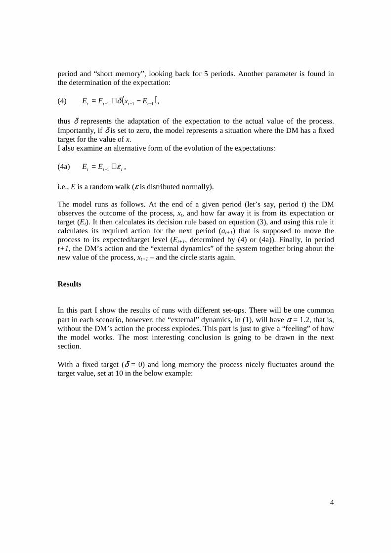
i.e., E is a random walk (ε is distributed normally). The model runs as follows. At the end of a given period (let’s say, period t) the DM observes the outcome of the process, xt, and how far away it is from its expectation or target (Et). It then calculates its decision rule based on equation (3), and using this rule it calculates its required action for the next period (at+1) that is supposed to move the process to its expected/target level (Et+1, determined by (4) or (4a)). Finally, in period t+1, the DM’s action and the “external dynamics” of the system together bring about the new value of the process, xt+1 – and the circle starts again. Results In this part I show the results of runs with different set-ups. There will be one common part in each scenario, however: the “external” dynamics, in (1), will have α = 1.2, that is, without the DM’s action the process explodes. This part is just to give a “feeling” of how the model works. The most interesting conclusion is going to be drawn in the next section. With a fixed target (δ = 0) and long memory the process nicely fluctuates around the target value, set at 10 in the below example:
5
Figure 1: The actual value of the process with fixed expectation (which equals 10) and long memory
8.0
8.5
9.0
9.5
10.0
10.5
11.0
1 201 401 601 801 1001
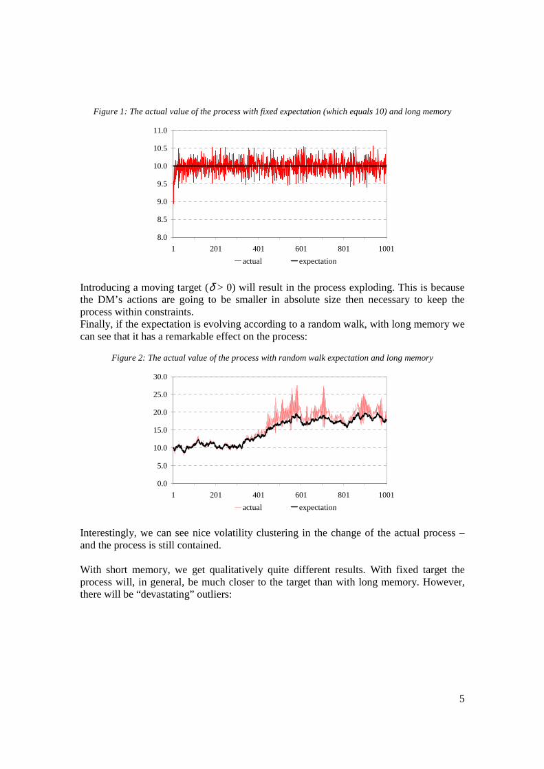
actual expectation Introducing a moving target (δ > 0) will result in the process exploding. This is because the DM’s actions are going to be smaller in absolute size then necessary to keep the process within constraints. Finally, if the expectation is evolving according to a random walk, with long memory we can see that it has a remarkable effect on the process:
Figure 2: The actual value of the process with random walk expectation and long memory
0.0
5.0
10.0
15.0
20.0
25.0
30.0
1 201 401 601 801 1001
actual expectation
Interestingly, we can see nice volatility clustering in the change of the actual process – and the process is still contained.
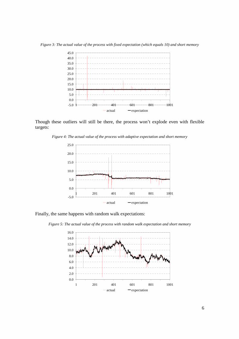
With short memory, we get qualitatively quite different results. With fixed target the process will, in general, be much closer to the target than with long memory. However, there will be “devastating” outliers:
6
Figure 3: The actual value of the process with fixed expectation (which equals 10) and short memory
-5.0
0.0
5.0
10.0
15.0
20.0
25.0
30.0
35.0
40.0
45.0
1 201 401 601 801 1001
actual expectation Though these outliers will still be there, the process won’t explode even with flexible targets:
Figure 4: The actual value of the process with adaptive expectation and short memory
-5.0
0.0
5.0
10.0
15.0
20.0
25.0
1 201 401 601 801 1001
actual expectation Finally, the same happens with random walk expectations:
Figure 5: The actual value of the process with random walk expectation and short memory
0.0
2.0
4.0
6.0
8.0
10.0
12.0
14.0
16.0
1 201 401 601 801 1001
actual expectation
7
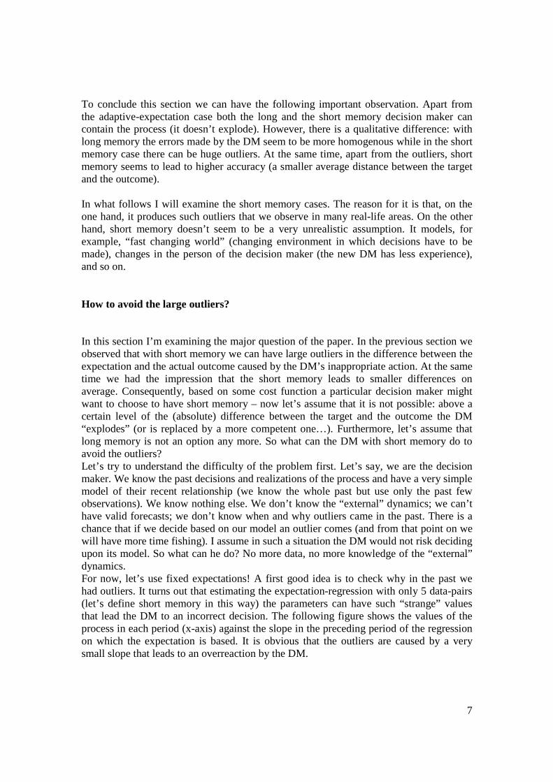
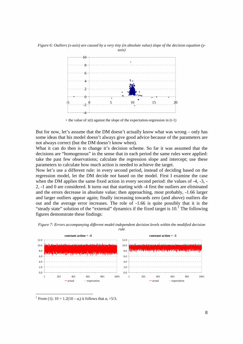
To conclude this section we can have the following important observation. Apart from the adaptive-expectation case both the long and the short memory decision maker can contain the process (it doesn’t explode). However, there is a qualitative difference: with long memory the errors made by the DM seem to be more homogenous while in the short memory case there can be huge outliers. At the same time, apart from the outliers, short memory seems to lead to higher accuracy (a smaller average distance between the target and the outcome). In what follows I will examine the short memory cases. The reason for it is that, on the one hand, it produces such outliers that we observe in many real-life areas. On the other hand, short memory doesn’t seem to be a very unrealistic assumption. It models, for example, “fast changing world” (changing environment in which decisions have to be made), changes in the person of the decision maker (the new DM has less experience), and so on. How to avoid the large outliers? In this section I’m examining the major question of the paper. In the previous section we observed that with short memory we can have large outliers in the difference between the expectation and the actual outcome caused by the DM’s inappropriate action. At the same time we had the impression that the short memory leads to smaller differences on average. Consequently, based on some cost function a particular decision maker might want to choose to have short memory – now let’s assume that it is not possible: above a certain level of the (absolute) difference between the target and the outcome the DM “explodes” (or is replaced by a more competent one…). Furthermore, let’s assume that long memory is not an option any more. So what can the DM with short memory do to avoid the outliers? Let’s try to understand the difficulty of the problem first. Let’s say, we are the decision maker. We know the past decisions and realizations of the process and have a very simple model of their recent relationship (we know the whole past but use only the past few observations). We know nothing else. We don’t know the “external” dynamics; we can’t have valid forecasts; we don’t know when and why outliers came in the past. There is a chance that if we decide based on our model an outlier comes (and from that point on we will have more time fishing). I assume in such a situation the DM would not risk deciding upon its model. So what can he do? No more data, no more knowledge of the “external” dynamics. For now, let’s use fixed expectations! A first good idea is to check why in the past we had outliers. It turns out that estimating the expectation-regression with only 5 data-pairs (let’s define short memory in this way) the parameters can have such “strange” values that lead the DM to an incorrect decision. The following figure shows the values of the process in each period (x-axis) against the slope in the preceding period of the regression on which the expectation is based. It is obvious that the outliers are caused by a very small slope that leads to an overreaction by the DM.
8
Figure 6: Outliers (x-axis) are caused by a very tiny (in absolute value) slope of the decision equation (y-axis)
-4
-2
0
2
4
6
8
10
-5 0 5 10 15 20
the value of x(t) against the slope of the expectation-regression in (t-1)
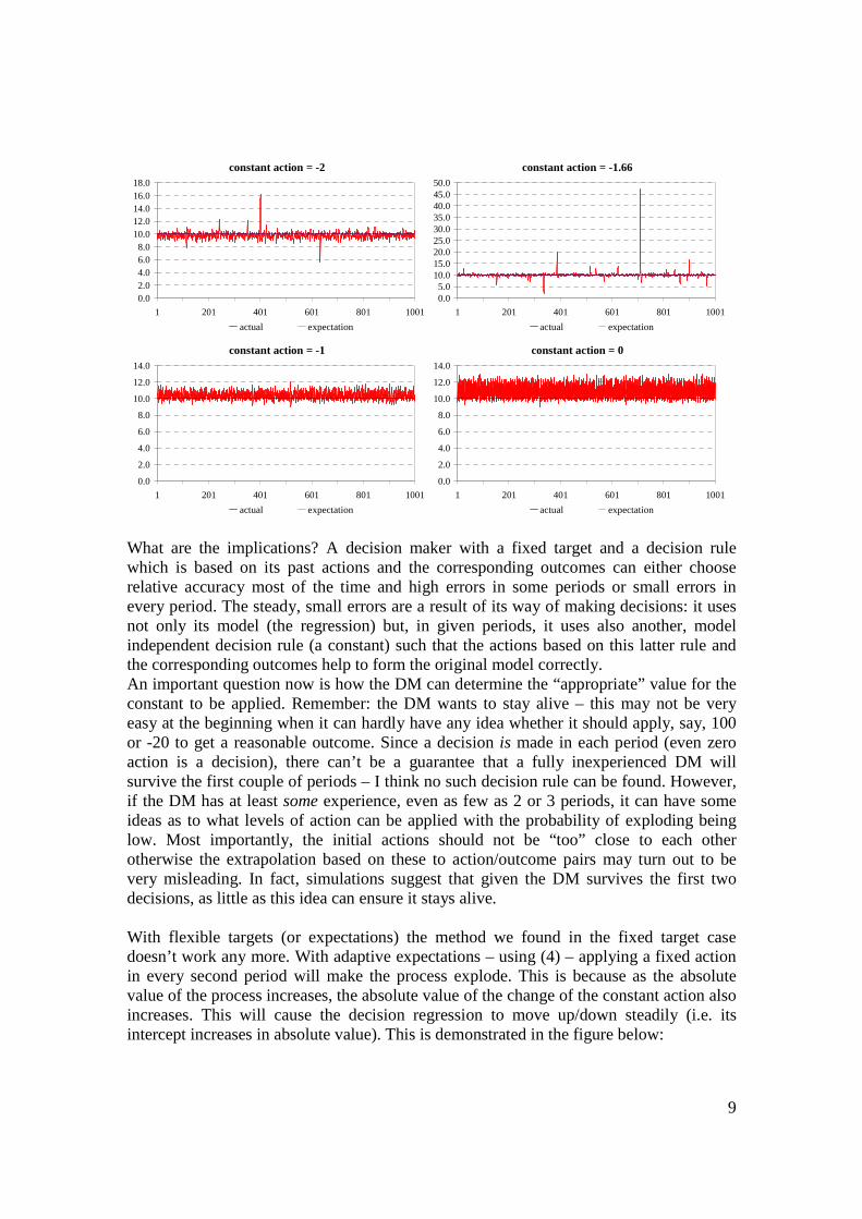
But for now, let’s assume that the DM doesn’t actually know what was wrong – only has some ideas that his model doesn’t always give good advice because of the parameters are not always correct (but the DM doesn’t know when). What it can do then is to change it’s decision scheme. So far it was assumed that the decisions are “homogenous” in the sense that in each period the same rules were applied: take the past few observations; calculate the regression slope and intercept; use these parameters to calculate how much action is needed to achieve the target. Now let’s use a different rule: in every second period, instead of deciding based on the regression model, let the DM decide not based on the model. First I examine the case when the DM applies the same fixed action in every second period: the values of -4, -3, -2, -1 and 0 are considered. It turns out that starting with -4 first the outliers are eliminated and the errors decrease in absolute value; then approaching, most probably, -1.66 larger and larger outliers appear again; finally increasing towards zero (and above) outliers die out and the average error increases. The role of -1.66 is quite possibly that it is the “steady state” solution of the “external” dynamics if the fixed target is 10.1 The following figures demonstrate these findings:
Figure 7: Errors accompanying different model-independent decision levels within the modified decision rule
constant action = -4
0.0
2.0
4.0
6.0
8.0
10.0
12.0
1 201 401 601 801 1001
actual expectation
constant action = -3
0.0
2.0
4.0
6.0
8.0
10.0
12.0
1 201 401 601 801 1001
actual expectation
1 From (1): 10 = 1.2(10 – at) it follows that at =5/3.
9
constant action = -2
0.02.04.06.08.0
10.012.014.016.018.0
1 201 401 601 801 1001
actual expectation
constant action = -1.66
0.05.0
10.015.020.025.030.035.040.045.050.0
1 201 401 601 801 1001
actual expectation constant action = -1
0.0
2.0
4.0
6.0
8.0
10.0
12.0
14.0
1 201 401 601 801 1001
actual expectation
constant action = 0
0.0
2.0
4.0
6.0
8.0
10.0
12.0
14.0
1 201 401 601 801 1001
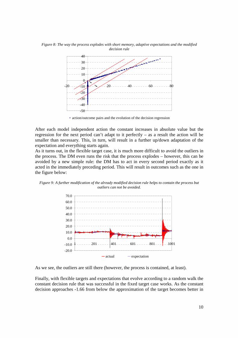
actual expectation What are the implications? A decision maker with a fixed target and a decision rule which is based on its past actions and the corresponding outcomes can either choose relative accuracy most of the time and high errors in some periods or small errors in every period. The steady, small errors are a result of its way of making decisions: it uses not only its model (the regression) but, in given periods, it uses also another, model independent decision rule (a constant) such that the actions based on this latter rule and the corresponding outcomes help to form the original model correctly. An important question now is how the DM can determine the “appropriate” value for the constant to be applied. Remember: the DM wants to stay alive – this may not be very easy at the beginning when it can hardly have any idea whether it should apply, say, 100 or -20 to get a reasonable outcome. Since a decision is made in each period (even zero action is a decision), there can’t be a guarantee that a fully inexperienced DM will survive the first couple of periods – I think no such decision rule can be found. However, if the DM has at least some experience, even as few as 2 or 3 periods, it can have some ideas as to what levels of action can be applied with the probability of exploding being low. Most importantly, the initial actions should not be “too” close to each other otherwise the extrapolation based on these to action/outcome pairs may turn out to be very misleading. In fact, simulations suggest that given the DM survives the first two decisions, as little as this idea can ensure it stays alive. With flexible targets (or expectations) the method we found in the fixed target case doesn’t work any more. With adaptive expectations – using (4) – applying a fixed action in every second period will make the process explode. This is because as the absolute value of the process increases, the absolute value of the change of the constant action also increases. This will cause the decision regression to move up/down steadily (i.e. its intercept increases in absolute value). This is demonstrated in the figure below:
10
Figure 8: The way the process explodes with short memory, adaptive expectations and the modified decision rule
-50
-40
-30
-20
-10
0
10
20
30
40
-20 0 20 40 60 80
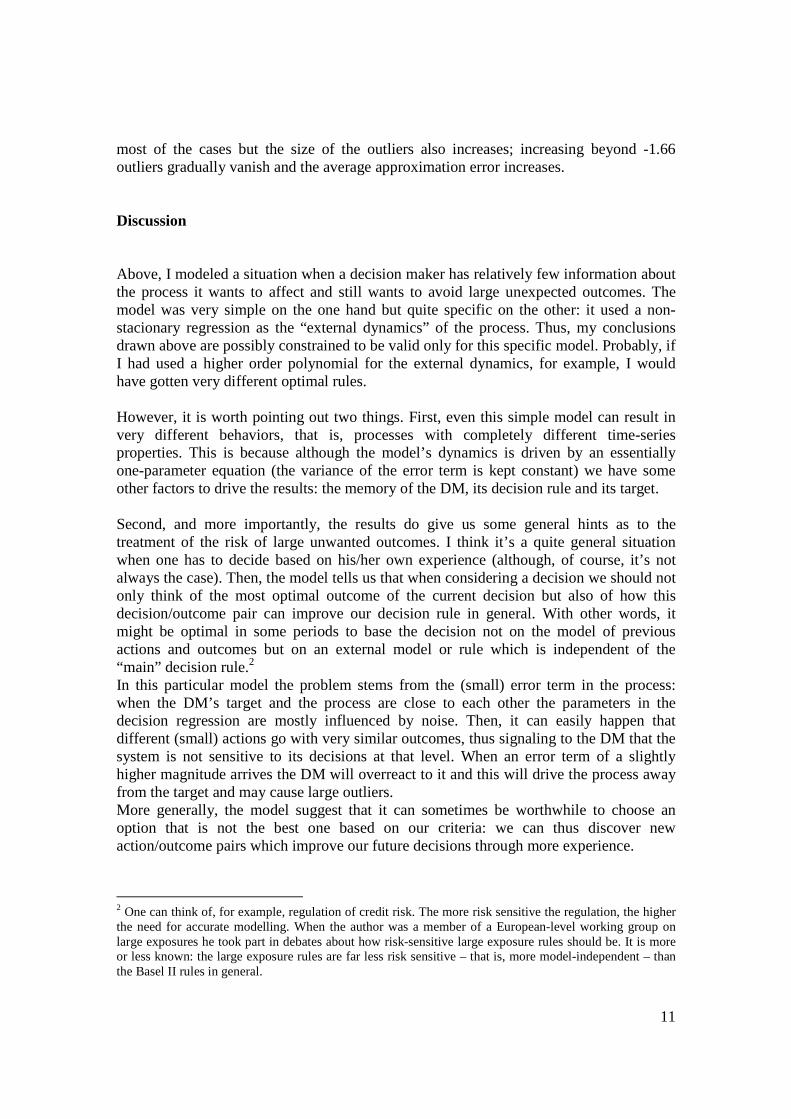
action/outcome pairs and the evolution of the decision regression After each model independent action the constant increases in absolute value but the regression for the next period can’t adapt to it perfectly – as a result the action will be smaller than necessary. This, in turn, will result in a further up/down adaptation of the expectation and everything starts again. As it turns out, in the flexible target case, it is much more difficult to avoid the outliers in the process. The DM even runs the risk that the process explodes – however, this can be avoided by a new simple rule: the DM has to act in every second period exactly as it acted in the immediately preceding period. This will result in outcomes such as the one in the figure below:
Figure 9: A further modification of the already modified decision rule helps to contain the process but outliers can not be avoided.
-20.0
-10.0
0.0
10.0
20.0
30.0
40.0
50.0
60.0
70.0
1 201 401 601 801 1001
actual expectation As we see, the outliers are still there (however, the process is contained, at least). Finally, with flexible targets and expectations that evolve according to a random walk the constant decision rule that was successful in the fixed target case works. As the constant decision approaches -1.66 from below the approximation of the target becomes better in
11
most of the cases but the size of the outliers also increases; increasing beyond -1.66 outliers gradually vanish and the average approximation error increases. Discussion Above, I modeled a situation when a decision maker has relatively few information about the process it wants to affect and still wants to avoid large unexpected outcomes. The model was very simple on the one hand but quite specific on the other: it used a non-stacionary regression as the “external dynamics” of the process. Thus, my conclusions drawn above are possibly constrained to be valid only for this specific model. Probably, if I had used a higher order polynomial for the external dynamics, for example, I would have gotten very different optimal rules. However, it is worth pointing out two things. First, even this simple model can result in very different behaviors, that is, processes with completely different time-series properties. This is because although the model’s dynamics is driven by an essentially one-parameter equation (the variance of the error term is kept constant) we have some other factors to drive the results: the memory of the DM, its decision rule and its target. Second, and more importantly, the results do give us some general hints as to the treatment of the risk of large unwanted outcomes. I think it’s a quite general situation when one has to decide based on his/her own experience (although, of course, it’s not always the case). Then, the model tells us that when considering a decision we should not only think of the most optimal outcome of the current decision but also of how this decision/outcome pair can improve our decision rule in general. With other words, it might be optimal in some periods to base the decision not on the model of previous actions and outcomes but on an external model or rule which is independent of the “main” decision rule.2 In this particular model the problem stems from the (small) error term in the process: when the DM’s target and the process are close to each other the parameters in the decision regression are mostly influenced by noise. Then, it can easily happen that different (small) actions go with very similar outcomes, thus signaling to the DM that the system is not sensitive to its decisions at that level. When an error term of a slightly higher magnitude arrives the DM will overreact to it and this will drive the process away from the target and may cause large outliers. More generally, the model suggest that it can sometimes be worthwhile to choose an option that is not the best one based on our criteria: we can thus discover new action/outcome pairs which improve our future decisions through more experience.
2 One can think of, for example, regulation of credit risk. The more risk sensitive the regulation, the higher the need for accurate modelling. When the author was a member of a European-level working group on large exposures he took part in debates about how risk-sensitive large exposure rules should be. It is more or less known: the large exposure rules are far less risk sensitive – that is, more model-independent – than the Basel II rules in general.
12
References Greenspan, A. (2008). We will never have a perfect model of risk. Financial Times, March 16, 2008 Rebonato, R. (2007). Plight of the Fortune Tellers: Why We Need to Manage Financial Risk Differently, Princeton University Press Sornette, D. (2003). Critical Market Crashes, http://arxiv.org/abs/cond-mat/0301543. Accessed on 10 February 2008. Taleb, N.N. (2004). Fooled by randomness. Penguin Books


