DSME 2021 Applied Econometrics for

Business DecisionsChapter 3: Simple Linear Regression

Part 1

Simple Linear RegressionObjective:

1. Use one (independent) variable to explain another (dependent) variable.

2. Model the relationship between the two variables as closed to the reality as possible.

2

Regression Modelling: Six-step Procedure

1. Identify the dependent and independent variables

2. Collect the sample data (Chapters 11 and Levine et al. Chapter 7)

3. Hypothesis the form of the model for E(y) (Chapter 3, 4 and 5)

4. Use the sample data to estimate unknown parameters in the model (Chapters 3 and 4)

5. Statistically check the usefulness of the model (Chapters 3, 4, 7 and 8)

6. When satisfied the model is useful, use it for prediction, estimation and so on. (Chapters 3 and 4)

3

Simple Linear Regression ModelRecall the general probabilistic model

y = E(y) +

The simple linear regression model

y = E(y) + = 0+ 1 x +

Deterministic component

Random error component

Interpretation of 0 & 1 4

Simple Linear Regression ModelSuppose the monthly sales revenue y is a function of the

monthly advertising expenditure x.

represents ALL unexplained variations in sales caused by (maybe) important but omitted variables or by unexplainable random phenomena.

As we make the standard assumption that the average of the random error is ZERO, i.e., E()=0, then the deterministic component of the straight-line probabilistic model represents the line of means E(y) = 0+ 1 x

5

y = E(y) +

0 1 2 3 4 5 6

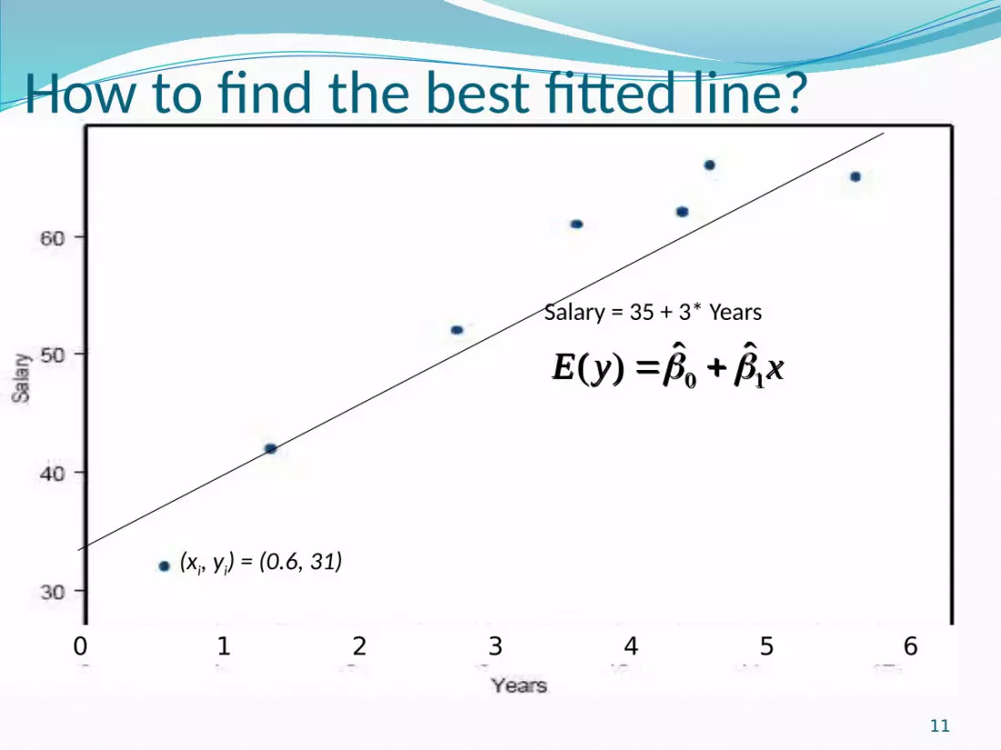
Salary = 35 + 3* Years

E(y) = 0 + 1 x

Interpretation of 0 & 1

Simple Linear Regression Model

6

Regression Modelling: Six-step Procedure

1. Identify the dependent and independent variables2. Collect the sample data (Chapters 11 and Levine et al. Chapter

7)3. Hypothesis the form of the model for E(y) (Chapter 3, 4 and 5)4. Use the sample data to estimate unknown parameters in the

model (Chapters 3 and 4)5. Statistically check the usefulness of the model (Chapters 3, 4, 7

and 8)6. When satisfied the model is useful, use it for prediction,

estimation and so on. (Chapters 3 and 4)

7

Population Sample estimates

Intercept

Slope

Error term1β̂

0β̂

1β

0β

eε

Population v.s. Sample

8

The hats can be read as ‘estimator of.’

1β̂

0β̂

1β

0β

eε

How to find the best fitted line? The fitted line from sample:

What is the best fitted line?Each predicted value as closed to the observed value as possible.

xββy 10ˆˆˆ

)ˆˆ(ˆ 10 ii xββy iy

From the fitted line

From the data

9

xββy 10ˆˆˆ

)ˆˆ(ˆ 10 ii xββy iy

How to find the best fitted line?

The extent to which the data points deviate from the lineCalled magnitude of the deviations / errors of prediction

Sum of errors (SE)

10

ˆ i i ie y y

i

ii

ii eyy )ˆ(

ˆ i i ie y y

i

ii

ii eyy )ˆ(

0 1 2 3 4 5 6

Salary = 35 + 3* Years

(xi, yi) = (0.6, 31)

xyE 10ˆˆ)(

11

How to find the best fitted line?

xyE 10ˆˆ)(

0 1 2 3 4 5 6

Salary = 35 + 3* Years

(xi, yi) = (0.6, 31)ei =-5.8

xyE 10ˆˆ)(

12

How to find the best fitted line?

0 1ˆ ˆ( ) 35 3*0.6 36.8E y x

xyE 10ˆˆ)(

0 1ˆ ˆ( ) 35 3*0.6 36.8E y x

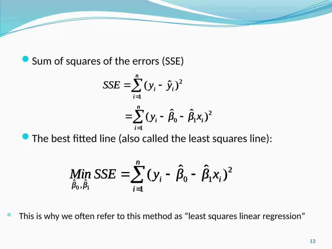
Sum of squares of the errors (SSE)

The best fitted line (also called the least squares line):

n

iii

n

iii

xββy

yySSE

1

210

1

2

)ˆˆ(

)ˆ(

n

iii

ββxββySSEMin

1

210ˆ,ˆ)ˆˆ(

10

This is why we often refer to this method as “least squares linear regression”

13

n

iii

n

iii

xββy

yySSE

1

210

1

2

)ˆˆ(

)ˆ(

n

iii

ββxββySSEMin

1

210ˆ,ˆ)ˆˆ(

10

The least squares regression always passes though the point

xβyβ

SS

rSSSS

xx

yyxxβ

x

y

xx

xyn

ii

n

iii

10

1

2

11

ˆˆ

ˆ

),( yx

Solving the minimization problem: Take partial derivatives with respect to and set equal to zero and solve.

Note: Sum of errors (SE) is always zero

1β̂0β̂

SD of Y

SD of X

14

xβyβ

SS

rSSSS

xx

yyxxβ

x

y

xx

xyn

ii

n

iii

10

1

2

11

ˆˆ

ˆ

),( yx

1β̂0β̂

Years of employment and salary ($1000) in 7 subjects:

Years Salary6.6 327.4 428.8 529.7 6110.5 6210.7 6611.8 65

Example: Salary Data

15

68.687.197.12962.0ˆ

1 β

962.0677.5

97.1287.13.5436.9

r

ssyx

y

x 19.836.968.63.54ˆ0

ŷ = -8.19 + 6.68x

Example: Salary Data (cont.)

1. Finding the linear regression line

2. Prediction

What is the wage if the working experience is 10 years?ŷ = -8.19 + 6.68*10 = 58.61

16

68.687.197.12962.0ˆ

1 β

962.0677.5

97.1287.13.5436.9

r

ssyx

y

x 19.836.968.63.54ˆ0

Recall: Numerical measure: CorrelationScatter plot is useful and important, but we still need a

numerical measure to supplement the graph.

Coefficient of Correlation r measures the direction and strength of the linear relationship between two quantitative variables.

17

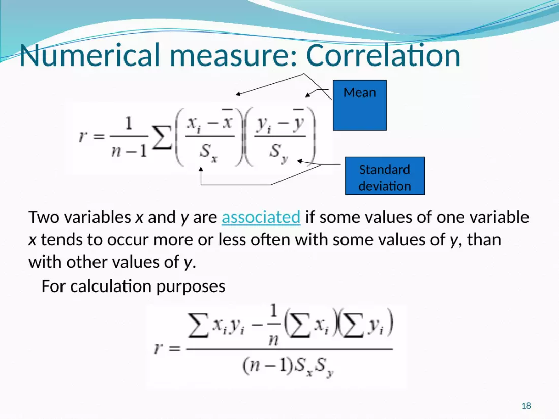
For calculation purposes

Standard deviation

Mean

Two variables x and y are associated if some values of one variable x tends to occur more or less often with some values of y, than with other values of y.

18

Numerical measure: Correlation

Properties of the correlation coefficient

19

r has no units -1 ≤ r ≤ 1 Sign indicates positive or negative correlation r = 1 implies perfect positive correlation or all data lie on a

line with positive slope. r = -1 implies perfect negative correlation or all data lie on a

line with negative slope. r only measures linear association; it doesn’t say anything

about non-linear patterns, no matter how strong

Do the Scatter Plot before undergoing regression

20

Correlation - Example

962.0677.5

11

y

i

x

i

Syy

Sxx

nr

21

962.0677.5

11

y

i

x

i

Syy

Sxx

nr

Exercise

22

We have four individuals in our dataset: John, Mary Paul and Peter.We want to see the correlation between study time and exam performance.i Study

Time (X)Exam scores (Y)

John 6 90Mary 5 80Paul 1 60Peter 1 50 r = 0.9709

25.3x

63.2xS70y

25.18yS

25.3x

63.2xS70y

25.18yS

An Example from Excel

23

Distance fr Fire Station (x)

Fire Damage (y)

3.4 26.21.8 17.84.6 31.32.3 23.13.1 27.55.5 360.7 14.13 22.3

2.6 19.64.3 31.32.1 241.1 17.36.1 43.24.8 36.43.8 26.1

摘要輸出迴歸統計

R 的倍數 0.960977715R 平方 0.923478169調整的 R 平方 0.917591874標準誤 2.316346184觀察值個數 15

ANOVA　 自由度 SS MS F 顯著值

迴歸 1 841.766358 841.7664

156.8862

1.25E-08殘差 13 69.75097535 5.36546

總和 14 911.5173333　 　 　　 係數 標準誤 t 統計 P- 值 下限

95%上限 95%

截距 10.27792855 1.420277811 7.236562

6.59E-06

7.209605

13.34625

X 變數 1 4.919330727 0.392747749 12.52542

1.25E-08

4.070851

5.767811

An Example from Excel

24

0 1 2 3 4 5 6 705

101520253035404550

X 變數 1 樣本迴歸線圖

Y預測 Y

X 變數 1

Y

An Example from Excel =4.92 implies that the estimated mean damage

increases by $4,920 for each additional mile from the fire station.

= 10.28 has the interpretation that a fire 0 miles from the fire station has an estimated mean damage of $10,280. But is it correct/meaningful?

Extrapolationextending the results beyond where you have data Example: If it takes you 2 seconds to put together a 2-piece jigsaw

puzzle, will it take you 3600 seconds (which is 1 hour) to put together a 3600-piece puzzle?!

25

1̂

0̂

1̂

0̂

Interpretation of CoefficientsRemember that the coefficients are only estimates based on

the sample – their values will typically change in repeated sampling.

How much confidence do we have that the estimated slope accurately approximates the true one?

It requires statistical inference in the form of confidence intervals and hypothesis testing.

26

27