A Solution to the Curse of DimensionalityProblem in Pairwise Scoring Techniques

Man-Wai Mak1 and Sun-Yuan Kung2

1 Center for Multimedia Signal Processing,Dept. of Electronic and Information Engineering,The Hong Kong Polytechnic University, China

enmwmak@polyu.edu.hk?

2 Dept. of Electrical Engineering, Princeton University, USAkung@princeton.edu

Abstract. This paper provides a solution to the curse of dimensionalityproblem in the pairwise scoring techniques that are commonly used inbioinformatics and biometrics applications. It has been recently discov-ered that stacking the pairwise comparison scores between an unknownpatterns and a set of known patterns can result in feature vectors withnice discriminative properties for classification. However, such techniquecan lead to curse of dimensionality because the vectors size is equal tothe training set size. To overcome this problem, this paper shows thatthe pairwise score matrices possess a symmetric and diagonally dominantproperty that allows us to select the most relevant features independentlyby an FDA-like technique. Then, the paper demonstrates the capabilityof the technique via a protein sequence classification problem. It wasfound that 10-fold reduction in the number of feature dimensions andrecognition time can be achieved with just 4% reduction in recognitionaccuracy.Keywords: Feature selection; Fisher discriminant analysis; curse of di-mensionality; protein sequence analysis; subcellular localization; supportvector machines.

1 Introduction

In computational biology, the subcellular location and structural family of aprotein provide important information about its biochemical functions. However,experimental analysis of proteins is time-consuming and cannot be performedon genome-wide scales. Therefore, a reliable and efficient method is essential forautomating the prediction of proteins’ subcellular locations and the classificationof protein sequences into functional and structural families.

It has been found that converting variable-length protein sequences to fixed-length feature vectors via preprocessing techniques can improve the accuracy? This work was supported by The Hong Kong Polytechnic University, Grant No.

APH18 and the RGC of Hong Kong, Grant No. PolyU5230/05E. The authors thankJian Guo for providing the pairwise alignment score matrices.

of subcellular localization and protein classification. In most cases, the prepro-cessing is embedded in a kernel function to facilitate subsequence classificationby support vector machines (SVMs). For example, in SVM-Fisher [7], a hiddenMarkov model (HMM) is trained from examples of a protein family. Then, givenan unknown protein sequence, the derivative of the log-likelihood score for theprotein sequence with respect to each of the HMM parameters is computed.The composition of these derivatives (Fisher scores) form a fixed-length vector,which is to be classified by an RBF-SVM. In SVM-Pairwise [11], each trainingsequence is compared with all other training sequences to form a list of pair-wise alignment scores. These scores are then packed to form a feature vector. Inthe mismatch kernel [10], a set of subsequences of length k, namely k-grams, isdefined. A query sequence is compared with the k-grams to count the numberof times the k-grams appear in the sequence. The concatenation of the countscorresponding to all k-grams forms a feature vector.

While the sequence-based methods perform reasonably well in protein homol-ogy detection, they may not be able to capture sufficient information from thesequences to detect remote homology. To overcome this difficulty, profile-basedmethods have been actively investigated in recent years [3, 9, 13]. A profile is amatrix in which elements in a column specify the frequency of each amino acidappears in that sequence position. Given a sequence, a profile can be derivedby aligning it with a set of similar sequences. The similarity score between aknown and an unknown sequence can be computed by aligning the profile ofthe known sequence with that of the unknown sequence [13]. Because the com-parison involves not only two sequences but also their closely related sequences,the score is more sensitive to detecting weak similarity between protein families.Research has also found that profile alignment can achieve better performancethan sequence alignment in predicting subcellular locations [4].

The comparison of two temporal sequences are often hampered by the factthat the two sequences often have different lengths whether or not they belongto the same family. To overcome this problem, pairwise comparison between asequence with a set of known sequences has been a popular scheme for creatingfixed-size feature vectors from variable length sequences. Many of the methodsmentioned earlier (e.g., [4, 8, 11]) fall into this scheme. Although this pairwiseapproach can usually create feature vectors with better discriminative properties,it also has its own limitation. The main problem is that the feature dimensionis the same as the number of training patterns, c.f., Figure 1 where we have Ttraining patterns with vector dimension equal to T too. This creates a curse ofdimensionality, because for most biometric and bioinformatic applications, thetraining size could be very large. In fact, for the applications addressed in thispaper, they are in the range of several thousands. The downside of such a curseof dimensionality is that it could hurt both training and recognition speed.

An obvious solution to the curse of dimensionality problem is to reduce thefeature size and yet retaining the most important information critical for theclassification of the training patterns. Research has found that just over 10% ofthe profile contributes 90% of the total score for positive training sequences [9],

suggesting that some features are more relevant to the classification task thanthe others. The feature sized reduction can be accomplished via either findingprinciple subspace or via weeding out those less significant features. This papertakes the latter approach. Moreover, in this paper, the importance of each fea-ture is independently computed, unlike the subspace reduction schemes. Morespecifically, for each component in the feature vectors, the symmetric diver-gence between the densities of the feature values from the positive class andthe negative class is computed. Then, the features with symmetric divergencessignificantly greater than the mean divergence are selected. New feature vectorswith reduced dimension are then used to train SVM classifiers.

The paper is organized as follows. Section 2 outlines the sequence and profilealignment algorithms. Section 3 explains how the non-discriminative featurescan be weeded out to reduce the dimensionality of the feature vectors, whichare then classified by multi-class SVMs in Section 4. The feature selection tech-nique is evaluated in Section 5 where significant reduction in recognition time isdemonstrated.

2 Sequence Versus Profile Alignment

2.1 Local Pairwise Sequence Alignment

Pairwise sequence alignment has been widely used to compute the similaritybetween two DNA or two protein sequences. It attempts to find the best matchbetween two sequences by inserting some gaps into proper positions of the two se-quences. One of the most successful local pairwise sequence alignment algorithmis the Smith-Waterman algorithm [16]. Denote

D = {S(1), . . . , S(i), . . . , S(j), . . . , S(T )}as a training set containing T sequences. Here, the i-th protein sequence isdenoted as

S(i) = S(i)1 , S

(i)2 , . . . , S(i)

ni, 1 ≤ i ≤ T

where S(i)k ∈ A, which is the set of 20 amino acid symbols, and ni is the length

of S(i). Using the BLOSUM62 substitution matrix [5], a set of similarity scoresε′(S(i)

u , S(j)v ) between position u of S(i) and position v of S(j) can be obtained.

Then, based on these scores and the Smith-Waterman alignment algorithm, asequence alignment score ρ′(S(i), S(j)) can be obtained, which easily leads to anormalized alignment score:

ζ ′(S(i), S(j)) =ρ′(S(i), S(j))√

ρ′(S(i), S(i))ρ′(S(j), S(j)). (1)

To facilitate SVM classification, we can convert a variable-length sequenceS(i) into a fixed-length feature vector

ζ′(i) = [ζ ′(S(i), S(1)) . . . ζ ′(S(i), S(T ))]T (2)

by aligning S(i) with each of the sequences in the training set. A kernel innerproduct between S(i) and S(j) can then naturally be obtained as < ζ′(i), ζ′(j) >.This leads to a class of algorithms referred to as the SVM-pairwise methodadopted by [8, 11].

The sensitivity of detecting subtle local homogenous segments can be im-proved by replacing pairwise sequence alignment with pairwise profile alignment.In the next subsection, we will use the similarity scores of local pairwise profilealignment to generate fixed-length feature vectors for SVM classification.

2.2 Local Pairwise Profile Alignment

Following [15], here we use a protein sequence (called query sequence) as a seedto search and align homogenous sequences from the SWISSPROT 46.0 [2] pro-tein database using the PSI-BLAST program [1] with parameters h and j set to0.001 and 3, respectively. These aligned sequences share some homogenous seg-ments and belong to the same protein family. The aligned sequences are furtherconverted into two profiles to express their homogenous information: position-specific scoring matrix (PSSM) and position-specific frequency matrix (PSFM).Both PSSM and PSFM are matrices with 20 rows and L columns, where L isthe total number of amino acids in the query sequence. Each column of a PSSMrepresents the log-likelihood of the residue substitutions at the correspondingpositions in the query sequence [1]. The (i, j)-th entry of the matrix representsthe chance of the amino acid in the j-th position of the query sequence beingmutated to amino acid type i during the evolution process. A PSFM containsthe weighted observation frequencies of each position of the aligned sequences.Specifically, the (i, j)-th entry of a PSFM represents the possibility of havingamino acid type i in position j of the query sequence.

Let us denote the PSSM of S(i) and the PSFM of S(j) as

P(i) = [p(i)1 ,p(i)

2 , . . . ,p(i)ni

] and Q(j) = [q(j)1 ,q(j)

2 , . . . ,q(j)nj

]

respectively, where

p(i)r = [p(i)

r,1, p(i)r,2, . . . , p

(i)r,20]

T, 1 ≤ r ≤ ni,

q(j)s = [q(j)

s,1, q(j)s,2, . . . , q

(j)s,20]

T, 1 ≤ s ≤ nj .

We adopt the scoring function introduced by [13] to compute the similarity scorebetween p(i)

u , q(j)v , p(j)

v , and q(i)u :

ε(S(i)u , S(j)

v ) =20∑

h=1

(p(i)u,hq

(j)v,h + p

(j)v,hq

(i)u,h

),

which is then applied to the the Smith-Waterman algorithm to obtain the pro-file alignment score ρ(S(i), S(j)) (see [6] for details). The local pairwise profilealignment score is then normalized as follows:

ζ(S(i), S(j)) =ρ(S(i), S(j))√

ρ(S(i), S(i))ρ(S(j), S(j)). (3)

The normalization allows us to compare the alignment scores arising from ma-trices with different numbers of columns.

Similar to the sequence alignment introduced in Section 2.1, we convert avariable-length sequence S(i) into a fixed-length feature vector

ζ(i) = [ζ(S(i), S(1)) . . . ζ(S(i), S(T ))]T (4)

for SVM classification.

3 Dimensionality Reduction by Fisher Feature Selection

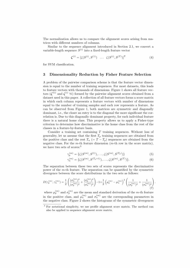
A problem of the pairwise comparison scheme is that the feature vector dimen-sion is equal to the number of training sequences. For most datasets, this leadsto feature vectors with thousands of dimensions. Figure 1 shows all feature vec-tors (ζ′(i) and ζ(i) ∀i) formed by the pairwise alignment scores obtained from adataset used in this paper. A collection of all feature vectors forms a score matrixin which each column represents a feature vectors with number of dimensionsequal to the number of training samples and each row represents a feature. Ascan be observed from Figure 1, both matrices are symmetric and diagonallydominant, i.e., the closer an entry is to the diagonal the more significant the cor-relation is. Due to this diagonally dominant property, for each individual featurethere is a natural home class. This property allows us to apply a Fisher-typecriterion to determine how discriminative is the home class from the rest of theclasses in a feature-by-feature basis.

Consider a training set containing T training sequences. Without loss ofgenerality, let us assume that the first Tp training sequences are obtained fromthe positive class and the rest Tn (= T − Tp) sequences are obtained from thenegative class. For the m-th feature dimension (m-th row in the score matrix),we have two sets of scores:3

γ(m)p = {ζ(S(m), S(1)), . . . , ζ(S(m), S(Tp))} (5)

γ(m)n = {ζ(S(m), S(Tp+1)), . . . , ζ(S(m), S(T ))}. (6)

The separation between these two sets of scores represents the discriminativepower of the m-th feature. The separation can be quantified by the symmetricdivergence between the score distributions in the two sets as follows:

D(γ(m)p , γ(m)

n ) =1

2

((σ

(m)n )2

(σ(m)p )2

+(σ

(m)p )2

(σ(m)n )2

)−1+

1

2

(µ(m)

p − µ(m)n

)2(

1

(σ(m)p )2

+1

(σ(m)n )2

).

(7)

where µ(m)p and σ

(m)p are the mean and standard derivation of the m-th feature

in the positive class, and µ(m)n and σ

(m)n are the corresponding parameters in

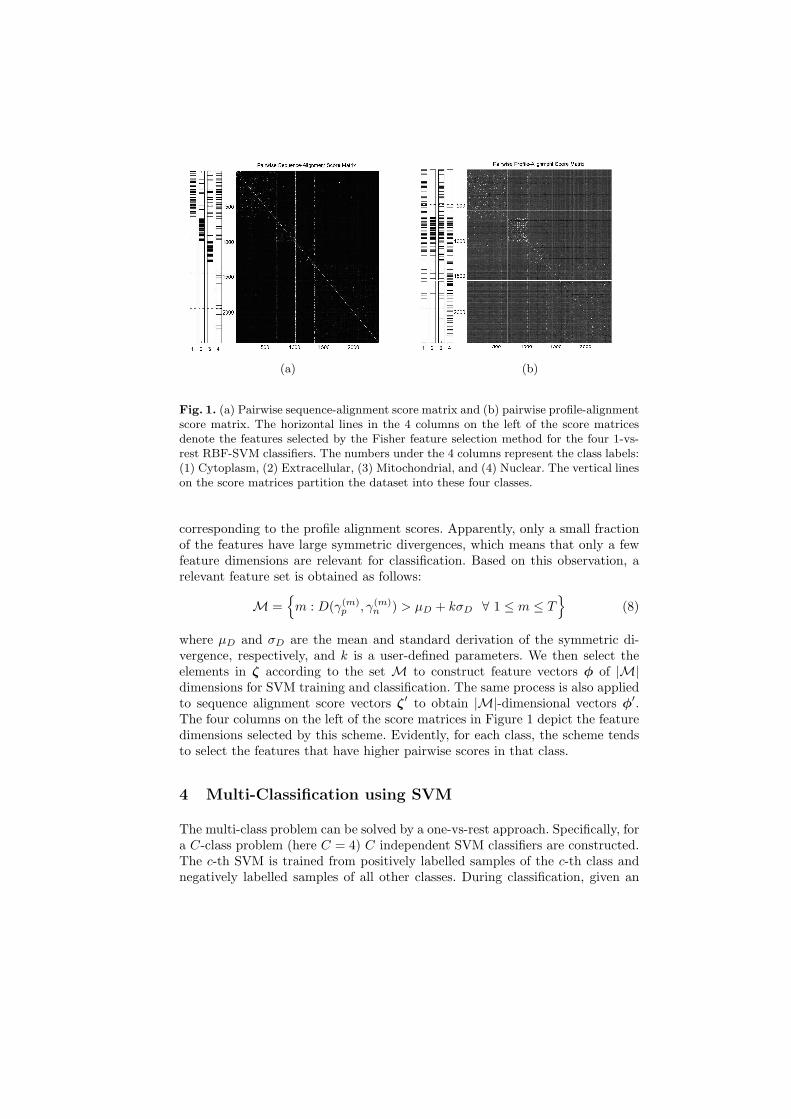
the negative class. Figure 2 shows the histograms of the symmetric divergences3 For notational simplicity, we use profile alignment score matrix. The method can

also be applied to sequence alignment score matrix.

(a) (b)

Fig. 1. (a) Pairwise sequence-alignment score matrix and (b) pairwise profile-alignmentscore matrix. The horizontal lines in the 4 columns on the left of the score matricesdenote the features selected by the Fisher feature selection method for the four 1-vs-rest RBF-SVM classifiers. The numbers under the 4 columns represent the class labels:(1) Cytoplasm, (2) Extracellular, (3) Mitochondrial, and (4) Nuclear. The vertical lineson the score matrices partition the dataset into these four classes.

corresponding to the profile alignment scores. Apparently, only a small fractionof the features have large symmetric divergences, which means that only a fewfeature dimensions are relevant for classification. Based on this observation, arelevant feature set is obtained as follows:

M ={

m : D(γ(m)p , γ(m)

n ) > µD + kσD ∀ 1 ≤ m ≤ T}

(8)

where µD and σD are the mean and standard derivation of the symmetric di-vergence, respectively, and k is a user-defined parameters. We then select theelements in ζ according to the set M to construct feature vectors φ of |M|dimensions for SVM training and classification. The same process is also appliedto sequence alignment score vectors ζ′ to obtain |M|-dimensional vectors φ′.The four columns on the left of the score matrices in Figure 1 depict the featuredimensions selected by this scheme. Evidently, for each class, the scheme tendsto select the features that have higher pairwise scores in that class.

4 Multi-Classification using SVM

The multi-class problem can be solved by a one-vs-rest approach. Specifically, fora C-class problem (here C = 4) C independent SVM classifiers are constructed.The c-th SVM is trained from positively labelled samples of the c-th class andnegatively labelled samples of all other classes. During classification, given an

0 0.5 1 1.50

200

400

600

800

1000

Symmetric DivergenceF

requ

ency

Cytoplasm

0 0.5 1 1.50

200

400

600

800

1000

Symmetric Divergence

Fre

quen

cy

Extracellular

0 0.5 1 1.50

200

400

600

800

1000

Symmetric Divergence

Fre

quen

cy

Mitochondrial

0 0.5 1 1.50

200

400

600

800

1000

Symmetric Divergence

Fre

quen

cy

Nuclear

Fig. 2. Histograms of the symmetric divergences between the profile alignment scoresof each positive class and its corresponding negative classes.

unknown protein sequence S, the output of the c-th SVM is computed as:

fc(S) =∑

i∈Sc

yc,iαc,iK(S, S(i)) + bc, (9)

where Sc is a set composed of the indexes of the support vectors, yc,i is the labelof the i-th sample, αc,i is the i-th Lagrange multiplier of the c-th SVM, and

K(S, S(i)) =

< ζ′, ζ′(i) > Sequence alignment using full features

< ζ, ζ(i) > Profile alignment using full features,

exp{−‖φ′ − φ′(i)‖2/σ2

}Sequence alignment using selected features

exp{−‖φ− φ(i)‖2/σ2

}Profile alignment using selected features

is the kernel function. Note that because the dimensionality of φ′ and φ isconsiderably smaller than that of ζ′ and ζ, it is possible to use RBF-SVMs toclassify φ′ and φ, whereas linear SVMs are chosen for classifying ζ′ and ζ to avoidcurse of dimensionality. Finally, the class of S is determined by a MAXNET:

y(S) = arg maxc

fc(S),

where y(S) is the predicted class of S. In the following, we refer y(S) with kernelK(·, ·) obtained from profile alignment to as pairwise profile alignment SVM (orsimply PairProSVM), and y(S) with kernel obtained from sequence alignmentto as pairwise sequence alignment SVM (PairSeqSVM).

5 Experiments and Results

Reinhardt and Hubbard’s eukaryotic protein dataset [14], which contains 2427amino acid sequences, was employed to test the performance of our method.The sequences in this dataset were extracted from SWISSPORT 33.0 and theirsubcellular locations (684 cytoplasm, 325 extracellular, 321 mitochondrial, and1097 nuclear proteins) have been annotated.

We used 5-fold cross validation for performance evaluation, i.e., the originaldataset was randomly divided into 5 subsets. Each subset was singled out inturn as a testing set, and the remaining ones were merged as the training set.The process was iterated 5 times until every subset has been used for testing.The prediction results from all iterations were averaged. The overall predictionaccuracy (OA), and the Matthew’s correlation coefficient (MCC) [12] were usedto assess the prediction result. MCC can overcome the shortcoming of usingaccuracy as a performance measure on unbalanced data. For example, in anunbalanced dataset where the majority of test samples belong to the positiveclass, a classifier predicting all samples as positive cannot be regarded as a goodclassifier if it fails to detect any negative samples. In such case, the MCC will bezero although the overall accuracy is high. Therefore, MCC is a better measurefor unbalanced classification.

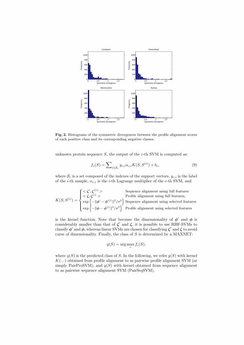
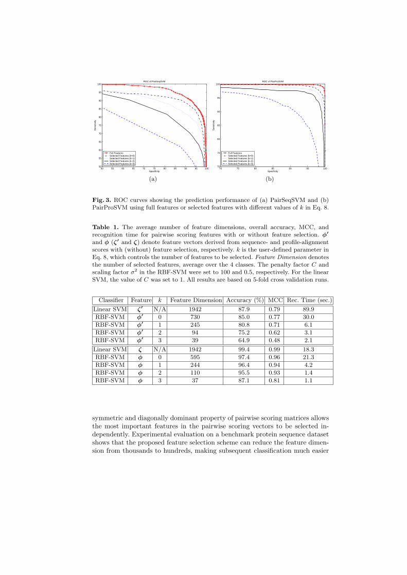
The prediction results of PairProSVM and PairSeqSVM are listed in Table 1.The overall accuracy of PairProSVM achieves 99.4%, which compares favorablywith PairSeqSVM (87.9%). This suggests that profile alignment provides moreinformation on subcellular location than sequence alignment. Also shown in Ta-ble 1 are the number of feature dimensions selected by the proposed featureselection scheme and the corresponding recognition time. Evidently, about 10-fold reduction in the number of feature dimensions can be achieved withoutjeopardizing the overall accuracy and MCC significantly. This dimensionalityreduction not only solves the curse of dimensionality problem but also leadsto about 10-fold reduction in recognition time. Figure 3 shows the ROC perfor-mance of PairSeqSVM and PairProSVM with and without feature selection. Theresults show that the performance progressively degrades when the value of k inEq. 8 increases. However, the amount of performance degradation (especially inPairProSVM) is not very significant when k is small.

Although fast recognition may not be critical for bioinformatics because se-quence classification can be done off-line, it is critically important for biomet-rics where real-time recognition is required. Therefore, the feature reductiontechniques proposed in this paper is potentially useful for reducing the cost ofbiometric systems.

6 Conclusions

A novel method to speed up the recognition of pairwise scoring features has beenpresented. The method can also alleviate the curse of dimensionality problemcommonly encountered in the pairwise scoring techniques. It was found that the

50 55 60 65 70 75 80 85 90 95 10050

55

60

65

70

75

80

85

90

95

100

Specificity

Sen

sitiv

ity

ROC of PairSeqSVM

Full FeaturesSelected Features (k=0)Selected Features (k=1)Selected Features (k=2)Selected Features (k=3)

70 75 80 85 90 95 10070

75

80

85

90

95

100

Specificity

Sen

sitiv

ity

ROC of PairProSVM

Full FeaturesSelected Features (k=0)Selected Features (k=1)Selected Features (k=2)Selected Features (k=3)

(a) (b)

Fig. 3. ROC curves showing the prediction performance of (a) PairSeqSVM and (b)PairProSVM using full features or selected features with different values of k in Eq. 8.

Table 1. The average number of feature dimensions, overall accuracy, MCC, andrecognition time for pairwise scoring features with or without feature selection. φ′

and φ (ζ′ and ζ) denote feature vectors derived from sequence- and profile-alignmentscores with (without) feature selection, respectively. k is the user-defined parameter inEq. 8, which controls the number of features to be selected. Feature Dimension denotesthe number of selected features, average over the 4 classes. The penalty factor C andscaling factor σ2 in the RBF-SVM were set to 100 and 0.5, respectively. For the linearSVM, the value of C was set to 1. All results are based on 5-fold cross validation runs.

Classifier Feature k Feature Dimension Accuracy (%) MCC Rec. Time (sec.)

Linear SVM ζ′ N/A 1942 87.9 0.79 89.9

RBF-SVM φ′ 0 730 85.0 0.77 30.0

RBF-SVM φ′ 1 245 80.8 0.71 6.1

RBF-SVM φ′ 2 94 75.2 0.62 3.1

RBF-SVM φ′ 3 39 64.9 0.48 2.1

Linear SVM ζ N/A 1942 99.4 0.99 18.3

RBF-SVM φ 0 595 97.4 0.96 21.3

RBF-SVM φ 1 244 96.4 0.94 4.2

RBF-SVM φ 2 110 95.5 0.93 1.4

RBF-SVM φ 3 37 87.1 0.81 1.1

symmetric and diagonally dominant property of pairwise scoring matrices allowsthe most important features in the pairwise scoring vectors to be selected in-dependently. Experimental evaluation on a benchmark protein sequence datasetshows that the proposed feature selection scheme can reduce the feature dimen-sion from thousands to hundreds, making subsequent classification much easier

and robust. With just a small reduction in recognition accuracy, a substantialspeed up in recognition time can be achieved.

References

1. S.F. Altschul, T.L. Madden, A.A. Schaffer, J. Zhang, Z. Zhang, W. Miller, andD.J. Lipman. Gapped blast and psi-blast: a new generation of protein databasesearch programs. Nucleic Acids Res., 25:3389–3402, 1997.

2. B. Boeckmann, A. Bairoch, R. Apweiler, M.C. Blatter, A. Estreicher, E. Gasteiger,M.J. Martin, K. Michoud, C. O’Donovan, I. Phan, S. Pilbout, and M. Schneider.The swiss-prot protein knowledgebase and its supplement trembl in 2003. NucleicAcids Res., 31:365–37, 2003.

3. S. Busuttil, J. Abela, and G.J. Pace. Support vector machines with profile-basedkernels for remote protein homology detection. Genome Informatics, 15(2):191–200, 2004.

4. J. Guo, M.W. Mak, and S.Y. Kung. Eukaryotic protein subcellular localizationbased on local pairwise profile alignment SVM. In IEEE Workshop on MachineLearning for Signal Processing, 2006.

5. S. Henikoff and J.G. Henikoff. Amino acid substitution matrices from proteinblocks. Proc. Natl. Acad. Sci., pages 10915–10919, 1992.

6. http://www.eie.polyu.edu.hk/∼mwmak/BSIG/PairProSVM.htm.7. T. Jaakkola, M. Diekhans, and D. Haussler. A discriminative framework for de-

tecting remote protein homologies. J. Comput. Biol., 7:95–114, 2000.8. J.K. Kim, G.P.S Raghava, S.Y. Bang, and S. Choi. Prediction of subcellular local-

ization of proteins using pairwise sequence alignment and support vector machine.Pattern Recog. Lett., 2006.

9. R. Kuang, E. Ie, K. Wang, K. Wang, M. Siddiqi, Y. Freund, and C. Leslie. Profile-based string kernels for remote homology detection and motif extraction. J. Bioin-fom. Comput. Biol., 3:527–550, 2005.

10. C.S. Leslie, E. Eskin, A. Cohen, J. Weston, and W.S. Noble. Mismatch stringkernels for discriminative protein classification. Bioinformatics, 20(4):467–476,2004.

11. L. Liao and W.S. Noble. Combining pairwise sequence similarity and supportvector machines for detecting remote protein evolutionary and structural relation-ships. J. Comput. Biol., 10(6):857–868, 2003.

12. B.W. Matthews. Comparison of predicted and observed secondary structure of t4phage lysozyme. Biochim. Biophys. Acta, 405:442–451, 1975.

13. H. Rangwala and G. Karypis. Profile-based direct kernels for remote homologydetection and fold recognition. Bioinformatics, 21(23):4239–4247, 2005.

14. A. Reinhardt and T. Hubbard. Using neural networks for prediction of the sub-cellular location of proteins. Nucleic Acids Res., 26:2230–2236, 1998.

15. L Rychlewski, B Zhang, and A. Godzik. Fold and function predictions for my-coplasma genitalium proteins. Fold Des., 3(4):229–238, 1998.

16. T.F. Smith and M.S. Waterman. Comparison of biosequences. Adv. Appl. Math.,2:482–489, 1981.