Seediscussions,stats,andauthorprofilesforthispublicationat:https://www.researchgate.net/publication/228574770

Astatisticallyprincipledapproachtohistogramsegmentation

ARTICLE·JANUARY2004

CITATIONS

4

READS

36

2AUTHORS,INCLUDING:

EricPauwels

CentrumWiskunde&Informatica

92PUBLICATIONS1,153CITATIONS

SEEPROFILE

Allin-textreferencesunderlinedinbluearelinkedtopublicationsonResearchGate,

lettingyouaccessandreadthemimmediately.

Availablefrom:EricPauwels

Retrievedon:04February2016

A Statistically Principled Approach to

Histogram Segmentation

Greet Frederix

Hogeschool Limburg, Universitaire Campus, B-3590 Diepenbeek, Belgium

Eric J. Pauwels

CWI, Kruislaan 413, 1098 SJ Amsterdam, The Netherlands

Abstract

This paper outlines a statistically principled approach to clustering one dimensionaldata. Given a dataset, the idea is to fit a density function that is as simple aspossible, but still compatible with the data. Simplicity is measured in terms of astandard smoothness functional. Data-compatibility is given a precise meaning interms of distribution-free statistics based on the empirical distribution function.

The main advantages of this approach are that (i) it involves a single decision-parameter which has a clear statistical interpretation, and (ii) there is no need tomake a priori assumptions about the number or shape of the clusters.

Key words: Clustering, cluster-validation, histogram segmentation,distribution-free statistics, Occam’s Razor

Email addresses: greet.frederix@hogelimb.be (Greet Frederix),eric.pauwels@cwi.nl (Eric J. Pauwels ).

URL: http://www.cwi.nl/∼pauwels/research/ (Eric J. Pauwels ).

Preprint submitted to Elsevier Science 10 June 2004

1 Introduction and Overview

1.1 Introduction

The exponential increase in computational power on the one hand, and theexplosion of stored digital data on the other, have contributed to the enduringinterest in clustering and unsupervised learning. As a consequence, there is noshortage of clustering algorithms and cluster validity indices (see e.g. [11–13]and references therein). Nevertheless, it is fair to say that clustering remainsa challenging problem as there is no general consensus on how the numberand shape of clusters should be determined. The following simple exampleillustrate this point: when confronted with a multimodal data-set, it is quitecommon to try and fit a mixture of Gaussians densities. However, there isno guarantee that this model is appropriate for the data at hand, e.g. theunderlying distribution might fail to be generated by Gaussians. Moreover,even if Gaussians turn out to be a acceptable choice, one still needs to takerecourse to ad-hoc procedures to estimate the number of components in themixture.

In this paper we propose a statistically principled approach for the clusteringof 1-dimensional data. In essence, the method we put forward is a computa-tionally tractable version of Occam’s Razor: Select the simplest density that isstill compatible with the data. Compatibility is measured by statistically com-paring the empirical distribution function for the data with the distribution(i.e. cumulative density) of the proposed density. The amount of deviation be-tween these two can be measured in precise probabilistic terms and a clear-cutquantitative decision criterion can be formulated.

Admittedly, the restriction to 1-dimensional data might look rather limiting.The problem is, however, not without merit: There are plenty of situations inwhich histograms of 1-dimensional data crop up which then need partitioningby separating data using local density-minima. In this context, the proposedmethod can be seen as a principled way to extract data-driven segmentationthresholds. Furthermore, the reason why the proposed solution is valid for1-dimensional data only, is that it hinges on the natural total ordering onthe real numbers. As such a total ordering is lacking for more-dimensionaldata, the algorithms detailed below cannot be implemented. Nevertheless,such data are amenable to cluster-methods that adhere, if not to the samealgorithms, at least to the same philosophy. For now however, we focus on theone-dimensional case.

It is important to point out that our proposal is motivated by what we seeas clear limitations in the more straightforward approaches to the histogram

2

segmentation problem. As this is most easily explained by means of a concreteexample, consider the histogram in Fig. 1 which was obtained by generatingthree Gaussians with different means, variances and sample sizes. Most peoplewould agree that the three clusters are fairly obvious and that the separation-thresholds should be positioned at about x = 2 and x = 7. If we now try and

Fig. 1. Histogram for 3 clusters

perform clustering by looking at the local minima of the histogram, we runinto a number of problems. First of all, local minima depend on the widthand position of the histogram bins. As there is no canonical way of choosingthese, this introduces a considerable amount of variability into the results. (Inour approach, we circumvent this problem, by using the empirical distribution(cumulative density) instead, as will be explained in Section 1.2.) But let usassume for the moment that the number and position of bins is considered tobe satisfactory. Then the next thing to do would be to inspect the local min-ima and decide whether or not they can be used as segmentation thresholds.However, even a cursory glance at Fig. 1 shows that for various reasons mostof these minima need to be discarded: a minimum might be too shallow (e.g.x ≈ 3 ) or too close to an even more pronounced one (e.g. x ≈ 5.5), or havetoo high a value (e.g. x ≈ 0), etc.

It therefore transpires that such a naive approach is fraught with difficultiesas it requires ad-hoc decisions to turn all sorts of handwaving indications (toohigh, too close, too shallow, etc) into crisp numerical thresholds. As will beexplained in the next subsection, the methodology proposed in this paper hasbeen designed to do away with the fuzziness in the procedure and to putforward a general and principled solution for this problem.

3

1.2 Outline of Proposed Method

Although the mathematical technicalities (see Sections 4 and 5) might appearinvolved, the underlying rationale for our approach is simple and intuitivelyappealing. In essence, we propose to fit a density function that is as simple aspossible, while still compatible with the data. The local minima of the resultingdensity are then taken to be the clustering thresholds.

More precisely, suppose we are given a sample x1, . . . , xn of 1-dimensionalobservations. Stripped down to its bare essentials, the proposed methodologyproceeds through the following steps to determine the number of clusters:

A: Use some technique to construct a tentative (“simple”) density f for thedata. (At this point, the actual technique used is largely irrelevant, one canuse splines or kernel-methods, or even some sort of “oracle”).

B: Once we have a candidate for f , we perform a simple statistical test tosee whether the data x1, . . . , xn support or refute the hypothesis expressedby the proposed f , i.e. in statistical parlance, we test a null-hypothesis H0

versus an alternative hypothesis H1, where· H0 : f is the true underlying density ;· H1 : f is NOT the underlying density ;The exact nature of the statistical test is not very important. In this paperwe will discuss the Kolmogorov-Smirnov (KS) or Cramer-von Mises (CvM)test in some detail, but other tests are conceivable;

C: If H0 is accepted, then there is no statistical reason to change the proposedestimate for f (unless we want to try an even simpler candidate!) and wecan use it to pinpoint the local minima (which then feature as cluster-separators). If the null-hypothesis is rejected, then we need to put forwarda different proposal for f .

1.3 Illustrative Example: Determining the Number of Components in a Gaus-sian Mixture

It’s probably helpful to illustrate this high-level step-by-step outline by meansof an example that is interesting in its own right: estimating the number ofcomponents for a Gaussian Mixture Model (GMM). Let’s return to the data inFig. 1 and let us assume that it’s known that these data have been generatedby a GMM. In such a case the data-analyst would simply put forward a GMMby combining Gaussian densities G(x; µ, σ) with mean µi and variance σ2

i ; theputative density f (referred to in step A) would therefore take the form:

f(x) =k∑

i=1

πiG(x; µi, σi). (1)

4

Clearly, in most realistic cases the number of components (k) would be un-known and determining it is in fact the main part of the problem. Indeed, oncethe number of Gaussians is fixed, one can take recourse to the well-knownExpectation-Maximization (EM) algorithm [5] to estimate the correspondingparameters (i.e. mean µi, variance σ2

i and prior probabilities πi for each group).

Typically, the data-analyst will try a number of possibilities and select theone that seems most appropriate. Our claim is that steps B and C allow us tocome up with a principled solution for this important (and often encountered)problem. More precisely, to get started we simply fit GMMk-models for anincreasing number of Gaussians k = 1, 2, 3, 4, etc. Adding more Gaussiansincreases the “complexity” of the model. As we are interested in the simplestmodel, we prefer the k-value to be as low as possible. To this end, we proceedto step B and test each putative model for its data-compatibility. To this end,we introduce the Kolmogorov-Smirnov (KS) distance between the proposedGMMk (for each fixed value of k) and the actual data. For the KS-distance,this amounts to:

dKS(Fn, F ) = supx∈IR

|Fn(x)− F (x)|. (2)

The empirical distribution function Fn is constructed from the sample (Fn(x)measures the fraction of observations not exceeding x) and the distribution Fis the integral of the estimated GMMk density function f (since f is a linearcombination of Gaussians, integration is straightforward). As an aside, noticethat the use of the empirical distribution function Fn rather than a histogram,sidesteps problems related to the number and shape of histogram-bins. TheKS-distances thus measures the discrepancy between the proposed densityand the data. The observed KS-distances dobs

KS for models with k Gaussiancomponents are shown in column 2 of Table 1.

For instance, for k = 2, the KS-distance equals 0.0754. From the definition(2) it’s clear that small values indicate a good correspondence between theproposed distribution and the data. Large values would cause rejection ofthe null-hypothesis that the proposed distribution is the true underlying dis-tribution. To turn this into an operational decision tool, we hark back tothe well-known Kolmogorov-Smirnov theorem which states that if F is thetrue underlying distribution of the data, the probability (p say) that the KS-distance exceeds a given distance δ, i.e. p ≡ P (dKS > δ |F is true), can becomputed independently of F (i.e. the KS-distance is distribution-free). Forinstance, the probability that dKS exceeds 0.0754 is approximately zero. Putdifferently, if GMM2 was the real underlying model, the observed data wouldbe extremely unlikely (have probability close to zero). The proposed GMM2

model is therefore (statistically) incompatible with the observed data.

5

Fig. 2. Determining the number of components k in a Gaussian mixture model us-ing the KS-distance (the data used in this experiment are displayed in Fig. 1). AGaussian mixture model is fitted for an increasing number of Gaussians: the resultsfor k = 2 (left) and k = 3 (right) are shown. First row: Proposed cumulative dis-tribution F superimposed on the the empirical distribution Fn. Second row: Plotof “residuals” |F − Fn| evaluated at the datapoints x1, x2, . . . , xn. For k = 2 themaximal value (i.e. the KS-distance) exceeds the critical value (horizontal line po-sitioned at δ0.5 = 0.828/

√n = 0.024; for more details, see paper). For k = 3 the

KS-distance is lower than the critical value which is indicative of a good fit. Thirdrow: Density of the resulting Gaussian mixture model.

On the other hand, fitting the GMM3 model (i.e. k = 3) results in a closerfit (see Fig. 2 right column) which means that the corresponding KS-distanceis significantly smaller (0.0138), and the probability of observing such a valueexceeds 0.5 (see section 3.3 for more details). In other words: assuming aGMM3 model, the actually observed values are extreme likely (i.e. the dataare statistically compatible with the proposed model).

Since the GMM2-model is not, while the GMM3-model is compatible withthe data, adherence to step C compels us to settle for k = 3 as the mostappropriate choice for the number of Gaussian components.

6

k dobsKS p-value

1 0.2034 < 10−4

2 0.0754 < 10−4

3 0.0138 0.9763

4 0.0136 0.9795

5 0.0106 0.9993

6 0.0105 0.9994Table 1For the data given in Fig. 1, a Gaussian mixture model is estimated as the number ofGaussians (k) ranges from 1 to 6. The observed KS-distance between the empiricaldistribution function of the actual data Fn and the estimated cumulative densityfunction F is provided in the second column. The last column shows the p-value forthe distance, i.e. p ≡ P (dKS > dobs

KS | k is correct).

1.4 Moving beyond GMMs: The Need for General Spline Models

In the previous subsection we explained how the general philosophy outlinedin section 1.2 yields a straightforward solution for determining the numberof components in Gaussian Mixture Model (GMM). However, this approachcan only be sanctioned if we are assured that data-generation mechanism doesindeed correspond to a mixture of Gaussians. In cases were such an assumptiondoesn’t hold, the above outlined simple procedure cannot be upheld. As anillustration, consider the bulky unimodal dataset in Fig. 3. The histogram isclock-shaped but the plateau is broader and flatter than that of a comparableGaussian (i.e. the density is platykurtic). As a consequence, fitting a singleGaussian will result in a poor fit, which can only be improved by adding asecond Gaussian (if one decides to stick to GMM-models). However, this wouldthen lead to the erroneous conclusion that there are two distinct clusters. Thereason for this unsatisfactory result is clear: the data-set wasn’t created bya Gaussian mixture in the first place, and we therefore should not insist onrestricting the choice of putative density models f to a GMM-family. Instead,as will be shown in section 4, we have to expand the class of candidates toincorporate more versatile spline-models.

This broadening of scope necessitates the setting up of a more sophisticatedmathematical framework, which we compels us to address the following twopoints:

(1) Choice of two particular statistical tests in step B: We willfocus our attention on the Kolmogorov-Smirnov (KS) and Cramer-vonMises (CvM) test-statistics as they make almost no assumptions on the

7

Fig. 3. Top left: Although clock-shaped this dataset is broader and flatter than atypical Gaussian. Top right: The spline-based non-parametric approach proposed inour paper correctly identifies the underlying unimodal (i.e. single cluster) density.Bottom: Fitting a GMM model results in the selection of 2 Gaussians, erroneouslysuggesting that there are two underlying clusters.

underlying density. This stands in contrast to lots of alternative testswhich assume that the underlying density is (approximately) Gaussian,or symmetric, or . . . etc. However, in many practical situations such priorassumptions are unwarranted. Therefore, to ensure the widest scope ofapplicability, we take recourse to general distribution-free tests such asCvM and KS. The critical values for these statistics are independent ofthe true underlying distribution that is being tested and can thereforebe computed in advance. In addition, these tests are based on the cu-mulative density (distribution) function F (x) =

∫ x−∞ f(u)du, rather than

on the density f itself, thus avoiding problems related to the choice ofhistogram parameters.

(2) Estimation of the putative density f : The bulk of the technicalwork in this paper is devoted to solving steps A and C. Rather than goingthrough the laborious process of suggesting a density, testing and thenchanging it, we show that standard spline theory allows us to take careof this process in a one step by solving a matrix optimization problem.More precisely, we show that the simplest (i.e. smoothest) density f thatwill still pass the hypothesis test (H0) in step B, can be obtained byfitting a spline to the data (rather than settling for a Gaussian mixture,or kernel density estimate, or something else). This solution is optimal inthat further smoothing of the density will result in statistical rejection of

8

H0. So in this very precise statistical sense, we can state that the densityf thus obtained, is the simplest possible that is still compatible with thedata, where:(a) simplicity is measured in terms of the standard smoothness functional

Φ(f) :=∫(f ′(x))2dx, which is an increasing function of the roughness

of the density.(b) data-compatibility of f is enforced by insisting that a statistical test

(such as KS or CvM) should not be able to reject f as a viable densityfor the observed data.

Let us now take a closer look at the procedure we propose to estimate thedensity. Suppose we have a sample x1, x2, . . . , xn from an unknown density f .First, we construct the empirical distribution function Fn(x) = #{xi |xi ≤x}/n (Fn makes a 1/n-jump at every observation xi). Clearly, Fn will be closeto the unknown cumulative density (distribution) function F (x) =

∫ x−∞ f(u)du,

and appropriate distance functions Dn = d(F, Fn) (such as the KS or CvMdistance) yield stochastic variables for which the probability density can becomputed explicitly (in Section 3 we will provide more details). In particular,it’s possible to compute how likely it is that Dn exceeds a predefined levelδ and it turns out that P (Dn > δ) is a (rapidly) decreasing function of thedifference δ since large deviations between F and Fn are exceptional. Next,we pick an acceptable level of statistical risk α (we will discuss this choice ofparameter in Section 3.3). Since the probability-distribution of Dn is known,one can compute for any given 0 < α < 1 the corresponding difference δα

such that P (Dn > δα) = α. In words: if F represents the correct underlyingdata-structure, then the probability that Dn = d(Fn, F ) will exceed δα is atmost α. Hence, α corresponds to what in statistics is called a Type-I-error,i.e. rejecting the null-hypothesis when in fact it’s correct.

Collecting the information above, the original problem can now be recast as aconstrained optimization problem: Given data x1, x2, . . . , xn construct Fn(x);next, find F that solves the constrained minimization problemmin Ψ(F ) where Ψ(F ) =

∫(F ′′(x))2 dx (simplicity)

subject to Dn = d(F, Fn) ≤ δα (data-compatibility)(3)

Once an optimal F is found, the corresponding density f = F ′ can be obtainedand clusters identified by locating local maxima and minima.

Overview of paper: In order to make further progress in solving (3), we needto specify the distance function and its probability distribution. This is done insection 3 where the Kolmogorov-Smirnov and Cramer-von Mises statistics arediscussed. Section 4 restates the optimization problem in more precise termsand section 5 reformulates the problem as a matrix optimization problem. The

9

reader not interested in technical details can skip the first part of that sectionand go to the computational solution scheme given in subsection 5.5. Finally,some experimental results are discussed in section 6.

2 Short Overview of Related Density-based Clustering Methods

Due to lack of space, this overview is kept as concise as possible and intendedonly to elucidate the connection between our proposal and the extensive classof established standard approaches to the problem. For more information onalternative techniques for clustering and density estimation, we refer the readerto excellent texts such as [6,10].

A first class comprises the parametric methods of which Gaussian MixtureModels (GMM) are the best-known exponent. The latter approach performssuperbly if and when the number of constituent Gaussian clusters is known,for then the EM algorithm [5] can be used to estimate the remaining number ofparameters. However, additional (and often ad-hoc) criteria must be invokedto estimate the actual number of clusters.

Non-parametric methods constitute an alternative approach in which noa priori assumption about the underlying density is put forward. In kerneldensity estimation, the dataset is convolved by a kernel-function (again of-ten a Gaussian) and the overall shape of the density is determined by thecharacteristic width of the kernel function. Now the problem is one of pickingthe appropriate kernel-width for which there are a number of theoretical re-sults (e.g. Parzen windowing). However, they do depend on knowledge aboutthe shape of the density, hence creating a recursion problem. Moreover, inmany cases better results are obtained if the width of kernel-function is madelocation dependent. But this further complicates the parameter estimationproblem.

Spline smoothers comprise another class of non-parametric density estima-tors. Most frequently, these appear under the guise of a penalized smoothingfunctional where for a set of observations (xi, yi), one needs to construct thedensity f that minimizes the functional:

Ψλ(f) =∫

(f ′′(x))2 dx + λ∑

(yi − f(xi))2. (4)

Notice however, that this functional (and hence the solution) depends on theweight-factor λ which only has a handwaving interpretation in terms of therelative importance of both penalty terms. As it turns out, the method thatwe propose in this paper is closely related to this penalized approach but ex-

10

changes the vagueness of the λ-parameter for an alternative with crisp prob-abilistic definition. In addition, there are some further subtle differences fora discussion of which we refer the interested reader to the CWI TechnicalReport [9].

3 Distribution-Free Statistics based on the Empirical Distribution

In this section we focus on two distribution-free statistics, both measuringthe deviation between the empirical distribution function Fn and its underly-ing model-distribution F . Recall that a statistic is called distribution-free if itsprobability distribution does not depend on the distribution of the true under-lying population. The distribution-free character of the Kolmogorov-Smirnovand Cramer-von Mises statistics is a consequence of the following elementarylemma.

Lemma 1 If X is a stochastic variable with distribution F and a continuousdensity f , then its image under F is uniformly distributed on the unit-interval[0, 1]:

U := F (X) ∼ U(0, 1) or again P (F (X) ≤ t) = t, (5)

for 0 ≤ t ≤ 1.

In particular, any sample X1, . . . , Xn drawn from F is mapped under F toan U(0, 1)-sample: Ui = F (Xi). Furthermore, the distribution function of thelatter can be expressed in terms of the original as Hn(t) = Fn(F−1(t)).

3.1 The Kolmogorov-Smirnov statistic

Our first candidate for Dn = d(Fn, F ) is the Kolmogorov-Smirnov statisticdefined as the L∞-distance between the empirical and the proposed distribu-tion:

dKS(Fn, F ) ≡ Kn := supx∈IR

|Fn(x)− F (x)|. (6)

Invoking Lemma 1 we can make the substitution t = F (x) and rewrite Kn interms that better elucidate the distribution-free character of the statistic, viz:

Kn = sup0≤t≤1

|Hn(t)− t| (7)

11

where as before, Hn is the empirical distribution of a U(0, 1)-sample of size n.For every δ > 0 one can explicitly compute the probability that Kn exceedsthe threshold δ (at least asymptotically for n −→∞, see eg. Durbin [7])

P (dKS(F, Fn) > δ) = QKS(√

n δ), (8)

where for x > 0

QKS(x) = 2∞∑

k=1

(−1)k+1e−2k2x2

. (9)

For ease of reference, we list the x-values that give rise to the most frequentlyused values for the cumulative denstiy FKS(x) = 1−QKS(x):

FKS(x) 0.05 0.10 0.25 0.50 0.75 0.90 0.95

x 0.5196 0.5712 0.6765 0.8276 1.0192 1.2238 1.3581

3.2 The Cramer-von Mises statistic

The original Cramer-von Mises statistic is defined as

dCvM(Fn, F ) ≡ W 2n := n

∫IR

(Fn(x)− F (x))2dF (x). (10)

Again, the distribution-free nature of this statistic is better explicified by thesubstitution t = F (x):

W 2n = n

1∫0

(Hn(t)− t)2 dt. (11)

As was the case for the Kolmogorov-Smirnov statistic (see (8)), it is possible togive an explicit expression for the p-value of the asymptotic statistic. Andersonand Darling [2] showed that limn→∞ P (W 2

n ≤ δ) = P (W 2 ≤ δ) equals

FCvM(δ) ≡ 1

π√

δ

∞∑k=0

(−1)k

(−1/2

k

)√4k + 1 e−βk(δ)K1/4(βk(δ)) (12)

where βk(x) = (4k + 1)2/(16x) and Kν(x) is the modified Bessel-function ofthe second kind (see [1] p. 376, # 9.6.23). The series expansion in (12) is

12

rapidly converging so that a few terms suffice to give an sufficiently accuratevalue for the p-value. The following table shows the values that under FCvMgive rise to the most frequently used p-values.

FCvM(x) 0.05 0.10 0.25 0.50 0.75 0.90 0.95

x 0.0366 0.0460 0.0702 0.1189 0.2094 0.3473 0.4614

Note that the p-values detailed above are asymptotic values, strictly speakingvalid only when the sample-size n tends to infinity. But simulation experi-ments show that for samples of size n > 100 these asymptotic values are quiteaccurate.

3.3 Choosing the α-threshold

We are now in a position to give a more detailed discussion of the choice ofthe α-parameter. Its significance is most easily explained for the Kolmogorov-Smirnov statistic. Recall from (3) that we choose the threshold δα such that

P (dKS(Fn, F ) ≤ δα) = 1− α,

or equivalently:

P (∀x : Fn(x)− δα ≤ F (x) ≤ Fn(x) + δα) = 1− α.

Hence the bounds Fn(x) ± δα provide a (1 − α) × 100% confidence intervalfor the real underlying distribution F . A small value for α will result in awide confidence-band with a high covering probability. As a consequence, onemight be tempted to settle for a small α-value (e.g. α = 0.1). However, therequirement for high coverage confidence needs to be balanced by the need forstatistical power to detect alternatives.

Indeed, a very wide confidence band will basically accommodate any choice ofF and we could always pick F to represent a simple unimodal density. Thisway, the constrained optimization principle becomes vacuous. The reason isclear: small values of α maximize the probability that the true underlyingdistribution is covered, but minimize the likelihood that a real difference willbe detected. This will be illustrated by the experiments in Section 6.2.

There is another way to see this. Suppose we pick a small α (say 0.1) andconstruct F that is as smooth as possible and still satisfies dKS(F, Fn) =sup

x|Fn(x)− F (x)| = δα. In particular, this entails that

P (supx|Fn(x)− F (x)| > δα |Fn is based on sample from F ) ≤ α = 0.1

13

This means that we put forward an underlying probability F such that theobserved sample is exceptional (in fact, has a probability of less than α = 0.1of being observed!). Clearly, this is an unsatisfactory state of affairs as weprefer a choice of F that would make the observed sample typical rather thanexceptional.

A similar argument can be used to argue against a very large value for α (say0.9). For in such a case we put forward a density F such that

P (supx|Fn(x)− F (x)| < δα |Fn is based on sample from F ) ≤ 1− α = 0.1,

again an unlikely event. From these considerations it transpires that choosingα = 0.5 seems most reasonable. The experiments reported in section 6.2 willfurther buttress this point.

4 Occam’s Principle as a Constrained Minimization Problem

At this point we are in a position to reformulate the clustering algorithm (3)in much more precise terms. (Readers not interested in technical details, canskip most of the next two sections and go straight to section 5.5.)

(1) Use the data x1, . . . , xn to construct the empirical distribution Fn(x);(2) Pick a threshold p-value α (default value: α = 0.5);(3) Choose a distance function D(q)

n = dq(Fn, F ) (q = 1, 2) and computethe corresponding εq where• D(1)

n ≡ Kn = supx∈IR

|Fn(x) − F (x)| corresponds to the Kolmogorov-

Smirnov distance (6);• D(2)

n ≡ W 2n = n

∫IR(Fn(x) − F (x))2 dF (x) refers to the Cramer-von

Mises distance (10):(4) For the chosen q and α, compute δq(α) such that P (D(q)

n > δq(α)) = αusing (asymptotic) eqs. (8) or (12) as appropriate.

(5) Determine F by solving the following constrained optimization prob-lem:

minimize Ψ(F ) where Ψ(F ) =∫IR

(F ′′(x))2 dx (13)

subject to dq(Fn, F ) ≤ δq

14

In order to formulate a solution for equation (13) we first show how, thanks tothe monotonicity of the cumulative distribution, the constraints on F can bereformulated as a finite set of constraints at the distinct sample points. Indeed,for the KS distance, the condition sup

x∈IR|Fn(x)− F (x)| ≤ δ1 is equivalent to

vi ≤ F (xi) ≤ wi (14)

where vi = Fn(xi)−δ1 and wi = Fn(xi)+δ1−1/n. The presence of the 1/n-termis due to the definition of the cumulative distribution Fn as a right-continuousfunction which increases by 1/n at each sample-point xi.

Likewise, by performing a simple integration, the constraint on the Cramer-von Mises statistic W 2

n ≤ δ2 can be recast as

n∑i=1

(F (x(i))−

i− 1/2

n

)2

+1

12n≤ δ2 (15)

with x(i) the ordered sample-points. It thus becomes a discrete constraint ofthe form

n∑i=1

(F (xi)− yi)2 ≤ δ (16)

by introducing yi = (i− 1/2)/n and δ = δ2 − 1/(12n).

Since the constraints in (13) can be re-expressed as constraints in the observa-tion points, it follows that the constrained optimization problem is actually aspline optimization problem (which, to avoid confusion, we formulate for

15

a generic function g):

minimize S(g) ≡b∫

a

(g′′(x))2dx subject to Cω(x1, . . . , xn) (17)

where Cω(x1, . . . , xn) is one of the following classical constraints at thepoints a ≤ xi ≤ b, (i = 1, . . . , n):

C1. Smoothing problem:∑n

i=1(g(xi) − yi)2 ≤ δ for some predefined

δ > 0;C2. Box problem: vi ≤ g(xi) ≤ wi.

However, since we are looking for a solution in the class of distribution func-tions, we need to add two additional constraints:

CDF1 Monotone increasing: g′(x) ≥ 0;CDF2 Limit behaviour:

limx→−∞

g(x) = 0

limx→+∞

g(x) = 1;

These additional constraints will be discussed in more detail in section 5.4.

The optimization problem (17) is well-defined for W2[a, b], i.e. the class of func-tions defined on [a, b] with absolutely continuous first derivative and squareintegrable second derivative.

16

5 Solving the Constrained Minimization Problem

5.1 Reformulation as a standard quadratic optimization problem

It is well-known that the solution of (17), subject to (C1) or (C2), is a cubicspline. Recall that cubic splines are cubic polynomials glued together at the“knots” x1, . . . , xn to ensure continuity of g, g′ and g′′. The first and last spline-segment are linear as a result of the boundary conditions (for more details werefer to [4,8]). Furthermore, standard theory assures us that the space of cubicsplines on n points constitutes a n+2 dimensional vector space which impliesthat one can determine a set of q ≡ n + 2 basis-functions Bi(x) such that anycubic spline can be expressed as

g(x) =q∑

i=1

ciBi(x). (18)

Among all possible candidates for such a basis, B-splines are a popular choiceas they have a local support and are therefore numerically well-behaved.

Once the basis has been selected, the smoothness-functional can be re-expressedas

b∫a

(g′′(x))2dx =

b∫a

∑j

cjB′′j (x)

2

dx = ctΣc (19)

where c = (c1, . . . , cq)t and

Σ ∈ IRq×q with Σij =

b∫a

B′′i (x)B′′

j (x) dx. (20)

The constraints can be recast in a similar fashion by observing that the columnvector (g(xi))

ni=1 can be written as Tc where T ∈ IRn×q and Tij = Bj(xi). If

we denote y = (y1, . . . , yn)t, then the optimization problem equation (17) is

17

reduced to a matrix optimization problem:

minimize ctΣc over c, subject to either (21)

C1. Smoothing problem: ||Tc− y||2 ≤ δ;C2. Box problem: v ≤ Tc ≤ w.

5.2 Solution of the matrix optimization problem

The minimization problem (21) subject to the second constraint (C2) is astandard quadratic matrix optimization problem, i.e. a quadratic objectivefunction subject to linear inequality constraints. Hence, only the first con-straint (C1) needs further amplification. Clearly, we can assume that the min-imum is realised at the boundary of the closed ellipsoid about y specified by(C1). Indeed, from equation (19) it is obvious that Σ is non-negative defi-nite. Hence, suppose that c is a solution within the ellipsoid, then we canfurther reduce the quadratic objective function (21) by taking c∗ = ρc with0 < ρ < 1 such that c∗ lies on the boundary of the ellipsoid. Put differently,the inequality in (C1) can be turned into an equality without loss of generality.As a consequence, introducing a Lagrangian multiplier λ turns the constraintminimization (21.C1) into a Lagrangian function

L(c, λ) = ctΣc + λ||Tc− y||2. (22)

Each λ gives rise to a spline cλ with corresponding distance δλ = E(cλ) ≡||Tcλ − y||2. Iteratively updating λ yields the solution corresponding to thedistance δ. For fixed λ, a straightforward solution to (22) is obtained by solvingthe linear system:

(TtT + λ−1Σ) cλ = Tty. (23)

Notice that the coefficient matrix has dimensions q × q = (n + 2) × (n + 2).However, if there are many datapoints (say n > 100) there is no need to solvethe above large system as a simple approximation performs equally well. Thisis discussed next.

18

5.3 Implementation of approximative solution

If there are lots of data, there is no need to position a knot at every observeddatapoint. In fact, computational efficiency will be improved if we approximatethe original spline-solution with a spline having uniformly spaced (grid)pointst1, . . . , tp as knots, where typically, p is much smaller than the number ofdatapoints n.

Maintaining the notation c, this time however to express the expansion of theapproximate spline with respect to the (p + 2) basic B-splines defined on theuniformly spaced t-knots, the smoothing term still equals ctΣc, however thistime Σ ∈ IR(p+2)×(p+2). First, we discuss the optimization problem subject toconstraint (C1). The expression in the constraint remains E(c) = ||Tc− y||2with T ∈ IRn×(p+2) and Tij = Bj(xi) but this time the B-splines are defined onthe set of t-knots. Since typically p � n, the matrix T is strongly rectangularwith far more rows than columns.

Applying a QR-decomposition to this matrix yields T = QR where Q an×(p+2) matrix with orthonormal columns, and R a square upper-triangularmatrix of size (p + 2). Since TtT = RtQtQR = RtR it follows that equation(22) can be written as

ctΣc + λ||Rc− η||2 (24)

and equation (23) is reduced to simple square system of size (p + 2):

(RtR + λ−1Σ)cλ = Rtη (25)

where η = Qty ∈ IRp+2. Since the coefficient matrix is square, symmetric andstrictly positive-definite, the solution is straightforward.

In the case of constraint (C2), changing from datapoints to equi-distant grid-points is not completely adequate as constraint satisfaction on the reduced setdoes not imply similar compliance on the original. However, we can still usethe spline defined on the gridpoints with the corresponding box-constraintsand adjust the parameter δ in (27) until the original constraints are satisfied.So the reduced problem is

minimize ctΣc subject to v∗ ≤ T∗c ≤ w∗ (26)

with

v∗i = Fn(ti)− δ, w∗i = Fn(ti) + δ − 1

n, (27)

19

and

T∗ ∈ IRp×(p+2) where T∗ij = Bj(ti). (28)

5.4 Enforcing the additional constraints

When using B-splines as basis-functions the monotonicity condition (CDF1)can be translated into a finite number of linear constraints. We outline themain idea of this proposal which was originally proposed by Schwetlick andKunert [15].

Since g is a cubic spline, its derivative is a spline of degree 2. The coefficientsc = (c1, . . . , cn+2)

t of g with respect to the B-splines on the ordered datasetx1, . . . , xn are related to the coefficients d = (d1, . . . , dn+1)

t of its derivative g′

by a linear relationship: d = Ac where A = LM with M ∈ IR(n+1)×(n+2) andL ∈ IR(n+1)×(n+1) given by

M =

−1 1

. . . . . .

−1 1

, L = diag

(3

xi − xi−3

)

with i = 2, . . . , n + 2. Notice that we use the standard extended dataset forcubic splines which is obtained by adding two additional points to both theleft (x−1 and x0) and right (xn+1 and xn+2) endpoint of the original dataset.Moreover, if gridpoints rather than datapoints are used as knots, the numberof points n must be replaced by the number of gridpoints p and A becomes a(p + 1)× (p + 2) matrix.

Since all B-splines are positive, the constraint g′(x) ≥ 0 can be replacedby the stronger condition d = Ac ≥ 0. Introducing this extra condition tothe optimization problem (21) does not change its numerical (algorithmic)complexity as a quadratic optimization problem with linear constraints.

Finally, the 0-1-bounds for the cumulative distribution function can be easilyincorporated in the optimization problem by adding the constraints 0 ≤ g(x1)and g(xn) ≤ 1. In matrix-notation this amounts to 0 ≤ T1.c and Tn.c ≤ 1where T1. and Tn. denote the first and last T -row, respectively.

In summary, the minimization problem subject to constraint (C1) and these

20

extra conditions amounts to (for λ fixed):

minc

ct(Σ + λRtR)c− 2ληtRc (29)

subject to

Ac ≥ 0

T1.c ≥ 0

Tn.c ≤ 1

The quadratic optimization problem with constraint (C2) and the additionalconditions is

minc

ctΣc (30)

subject to

max(v∗,0) ≤ T∗c ≤ min(w∗,1)

Ac ≥ 0

The bounds v∗ and w∗ are adjusted to satisfy constraint (C2).

5.5 Overview of the computations

Spline density estimation based on Cramer-von Mises statistic

(1) Collect the data x1, . . . , xn.(2) Fix α and determine the corresponding δ2 using eq.(12) or the corre-

sponding pre-computed table. E.g. α = 0.5 yields δ2 = 0.119.(3) Compute y1, . . . , yn and δ as defined in equation (16).(4) Construct a grid t1, . . . , tp (for p = 50 say) on which the spline will be

defined.(5) Compute the matrices Σ ∈ IR(p+2)×(p+2) and T ∈ IRn×(p+2) as defined in

eq. (20). Apply a QR-decomposition on T and define η = Qty.(6) Propose the regression-line through (xi, yi) as the initial solution (λ =

0). Denote the coefficients of this line with respect to the basis of B-splines defined on the knots t1, . . . , tp by c0. If E(c0) = ||Tc0 − y||2 ≤ δ,

21

terminate the program.(7) Otherwise, increase λ. In each iteration-step, first solve the quadratic

optimization problem (29) for fixed λ to get the coefficients c. (Recall thatwe use an approximation by imposing a stronger monotonicity constraintthan is actually needed.) Then compute E(c) and stop if it’s close to δ.Then the spline at the knots ti with coefficients c is the solution of theproblem.

Spline density estimation based on Kolmogorov-Smirnov statistic

(1) Collect the data x1, . . . , xn.(2) Fix α and determine the corresponding δ1 using eq.(9) or the correspond-

ing pre-computed table. E.g. α = 0.5, yields δ1 = 0.828/√

n.(3) Define a grid t1, . . . , tp (p = 50) on which the B-splines B1, . . . , Bp+2 are

defined.(4) Compute the empirical distribution of the data at the gridpoints

Fn(t1), . . . , Fn(tp).(5) Compute the matrices Σ ∈ IR(p+2)×(p+2) and T∗ ∈ IRp×(p+2) as defined in

equation (28). These matrices are used in step 8.(6) Compute the empirical distribution of the data: Fn(x1), . . . , Fn(xn). Com-

pute the original bounds v(δ1) and w(δ1) as defined in equation (14) andthe matrix T ∈ IRn×(p+2) with Tij = Bj(xi). These computations are usedto check the constraint in step 9.

(7) Denote by δ0 an initial value to compute the bounds v∗i = Fn(ti)− δ0 andw∗

i = Fn(ti) + δ0 − 1/n.(8) Solve the quadratic optimization problem (30).(9) If the constraint v(δ1) ≤ Tc ≤ w(δ1) is satisfied, terminate the program.

Then the spline defined on the knots ti with coefficients c is the solutionof the problem.

(10) Otherwise decrease δ, recompute the bounds v∗i and w∗i and find the

solution of (30) with these bounds.

6 Experimental Results

6.1 Introductory example

Have another look at the historgram for the introductory example in Sec-tion 1.1. As can be seen from Fig. 4, the cluster-thresholds corresponding tothe local minima of the spline-density generated by the method proposed inthis paper, the clusters are separated in a intuitively acceptable way.

22

Fig. 4. The method proposed in this paper produces a spline-density with exactlytwo local minima. The corresponding thresholds are indicated on the histogram.

6.2 Experimental support for proposed choice of α threshold

In section 3.3 we argued that the α-parameter should be set equal to 0.5 sincewe want a typical rather than an exceptional density-model to fit the givendata. This way, we intend to strike a reasonable balance between the coveringprobability of the confidence interval on the one hand, and the power againstalternatives on the other. In this section we report on some experiments thatconfirm the appropriateness of this choice.

Example 1: In the first example, we generated 100 samples of size 1000from a Gaussian mixture distribution π1N(µ1, σ

21) + π2N(µ2, σ

22) where π1 =

π2 = 0.5, σ1 = σ2 = 1 and µ1 = 0 and µ2 = d; hence d is the separationbetween the two clusters which in our experiments varies from 2 to 4. Fig. 5shows some typical histograms of datasets drawn from the given distributionfor various values of d. We applied our histogram-segmentation method usingdifferent values for α on each of the generated datasets and stored the numberof extracted clusters. The results are summarized in Table 2. From Fig. 5 itis clear that the histogram begins to show bi-modality at around d = 2.5.This is picked up nicely when α = 0.5. Setting α = 0.1 however, resultsin a wide confidence band that accommodates an overly smooth (and henceunimodal) solution for F . The decision in favour of bi-modality is thereforepostponed until d ≥ 3. Conversely, fixing α = 0.9 increases data-fidelity andthe transition from 1 to 2 clusters occurs earlier (somewhere around 2.3).

23

α = 0.1 d=2 d=2.5 d=2.8 d=3 d=3.5 d=4

1 cluster 100 100 93 44 0 0

2 clusters 0 0 7 56 100 100

α = 0.5 d=2 d=2.5 d=2.8 d=3 d=3.5 d=4

1 cluster 100 76 16 0 0 0

2 clusters 0 24 84 100 100 100

α = 0.9 d=2 d=2.5 d=2.8 d=3 d=3.5 d=4

1 cluster 95 23 0 0 0 0

2 clusters 5 77 100 100 100 100Table 2The table displays for each distance d the number of samples for which our methodfound 1 or 2 clusters. To illustrate the appropriateness of setting α = 0.5 we alsolist the results for more extreme choices α = 0.1 (over-smoothing) and α = 0.9(under-smoothing).

24

−4 −3 −2 −1 0 1 2 3 4 50

10

20

30

40

50

60

70

−3 −2 −1 0 1 2 3 4 50

10

20

30

40

50

60

−3 −2 −1 0 1 2 3 4 5 60

10

20

30

40

50

60

−3 −2 −1 0 1 2 3 4 5 60

10

20

30

40

50

60

−3 −2 −1 0 1 2 3 4 5 60

10

20

30

40

50

60

−4 −2 0 2 4 6 80

10

20

30

40

50

60

70

−4 −2 0 2 4 6 80

10

20

30

40

50

60

70

−4 −3 −2 −1 0 1 2 3 4 5 60

10

20

30

40

50

60

−4 −2 0 2 4 6 80

10

20

30

40

50

60

70

−3 −2 −1 0 1 2 3 4 5 60

5

10

15

20

25

30

35

40

45

50

Fig. 5. Typical histograms of datasets in Section 6.2, Example 1. The samples ofsize 1000 taken from Gaussian mixture distributions 0.5N(0, 1) + 0.5N(d, 1), i.e.an equal mixture of two unit-variance Gaussians separated by a distance d. Eachrow shows two typical realisations for increasing distance: d grows from d = 2 (firstrow), over d = 2.5, d = 2.8 and d = 3 to d = 3.5 in the last row.

25

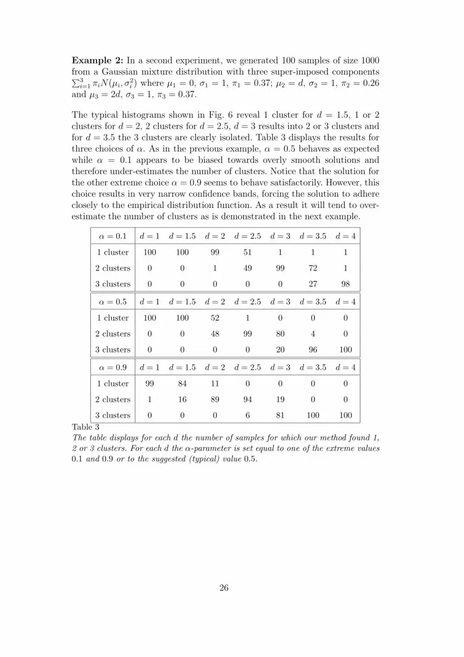
Example 2: In a second experiment, we generated 100 samples of size 1000from a Gaussian mixture distribution with three super-imposed components∑3

i=1 πiN(µi, σ2i ) where µ1 = 0, σ1 = 1, π1 = 0.37; µ2 = d, σ2 = 1, π2 = 0.26

and µ3 = 2d, σ3 = 1, π3 = 0.37.

The typical histograms shown in Fig. 6 reveal 1 cluster for d = 1.5, 1 or 2clusters for d = 2, 2 clusters for d = 2.5, d = 3 results into 2 or 3 clusters andfor d = 3.5 the 3 clusters are clearly isolated. Table 3 displays the results forthree choices of α. As in the previous example, α = 0.5 behaves as expectedwhile α = 0.1 appears to be biased towards overly smooth solutions andtherefore under-estimates the number of clusters. Notice that the solution forthe other extreme choice α = 0.9 seems to behave satisfactorily. However, thischoice results in very narrow confidence bands, forcing the solution to adhereclosely to the empirical distribution function. As a result it will tend to over-estimate the number of clusters as is demonstrated in the next example.

α = 0.1 d = 1 d = 1.5 d = 2 d = 2.5 d = 3 d = 3.5 d = 4

1 cluster 100 100 99 51 1 1 1

2 clusters 0 0 1 49 99 72 1

3 clusters 0 0 0 0 0 27 98

α = 0.5 d = 1 d = 1.5 d = 2 d = 2.5 d = 3 d = 3.5 d = 4

1 cluster 100 100 52 1 0 0 0

2 clusters 0 0 48 99 80 4 0

3 clusters 0 0 0 0 20 96 100

α = 0.9 d = 1 d = 1.5 d = 2 d = 2.5 d = 3 d = 3.5 d = 4

1 cluster 99 84 11 0 0 0 0

2 clusters 1 16 89 94 19 0 0

3 clusters 0 0 0 6 81 100 100Table 3The table displays for each d the number of samples for which our method found 1,2 or 3 clusters. For each d the α-parameter is set equal to one of the extreme values0.1 and 0.9 or to the suggested (typical) value 0.5.

26

−3 −2 −1 0 1 2 3 4 5 6 70

10

20

30

40

50

60

−3 −2 −1 0 1 2 3 4 5 6 70

10

20

30

40

50

60

−3 −2 −1 0 1 2 3 4 5 6 70

5

10

15

20

25

30

35

40

45

50

−4 −2 0 2 4 6 80

10

20

30

40

50

60

−4 −2 0 2 4 6 8 100

10

20

30

40

50

60

−4 −2 0 2 4 6 8 100

5

10

15

20

25

30

35

40

45

50

−4 −2 0 2 4 6 8 100

5

10

15

20

25

30

35

40

45

−4 −2 0 2 4 6 8 100

5

10

15

20

25

30

35

40

45

−4 −2 0 2 4 6 8 100

10

20

30

40

50

60

−4 −2 0 2 4 6 8 10 120

10

20

30

40

50

60

Fig. 6. Typical histograms of datasets in Section 6.2, Example 2. Sam-ples of size 1000 are taken from a 3-component Gaussian mixture0.37N(0, 1) + 0.26N(d, 1) + 0.37N(2d, 1), i.e. a mixture of two unit-varianceGaussians separated by a distance 2d, with a slightly smaller unit-Gaussian clusterin between. Each row shows two typical realisations for increasing separation: dgrows from d = 1.5 (first row), over d = 2, d = 2.5 and d = 3 to d = 3.5 in the lastrow.

27

Example 3: From the experiments reported above, one might be tempted tochoose a large value for α, e.g. α = 0.9. This, however, would be a mistake asthe covering probability 1−α would then become too small. As a consequence,the probability that the real underlying distribution is within the computedbounds is small (e.g. only 10% if we pick α = 0.9) and the proposed solutionwill be largely determined by the random fluctuations in the sample. Thistranspires from the next experiment in which we compare, for different valuesof α, the number of clusters found in a sample of size 1000 from a uniformU(0, 1) distribution (i.e. there is one real underlying cluster). We see that forα = 0.9 the number of clusters is over-estimated in about one third of theexperiments.

α = 0.1 α = 0.5 α = 0.9

1 cluster 100 96 66

2 clusters 0 4 28

3 clusters 0 0 6Table 4Number of clusters found by the proposed algorithm for different values of α. Eachsample of size 1000 is drawn from a uniform U(0, 1) sample (i.e. there is only onereal underlying cluster). In total, 100 experiments were performed. It transpires thatfor α = 0.9 the number of clusters is significantly overestimated, whereas α = 0.5has a very acceptable error-rate.

6.3 Application to Image Segmentation

We have applied the proposed 1-dimensional clustering method to the prob-lem of image segmentation, and we illustrate the results for both naturaland synthetic images (decoration designs). In all the experiments reportedbelow we used constraints based on the CvM distance function in combina-tion with α = 0.5. For more information we refer the interested reader tohttp://www.cwi.nl/∼pauwels/research/.

Natural images:

To accomplish segmentation, the pixels of an image can be mapped into anumber of colour spaces such as RGB, LAB or opponent-colours. A com-pletely data-driven alternative is provided by the principal components ob-tained via PCA analysis of the datapoints in RGB-space. To this end onemaps all the pixels into RGB space and performs a Principal ComponentAnalysis (PCA) on the resulting data-cloud. The first PCA component yieldsthe colour-combination that maximizes contrast, the second PCA-componentyields the best uncorrelated alternative, etc. The clusterings for each of the re-sulting histograms can easily be assigned a saliency score by checking whether

28

or not there is more than one cluster and if so, how well-separated and pro-nounced these clusters are (e.g. by comparing the distance between their meansto their variance). In the experiments reported below (see Figs. 7 and 8) wedisplay for each image one or two of the most salient histograms and thecorresponding clustering.

Decoration designs: These are synthetic and manually designed imagesthat need to be decomposed in foreground and background (to extract designmotifs). To avoid being misled by variations in the background, each imageis smoothed at a number of increasingly coarser scales. The smoothed imagesare transformed to the LAB-colour space and each projected dataset is clus-tered. This procedure is stopped as soon as our clustering-method presentstwo clusters. Some results are shown in Fig. 9.

7 Conclusions

In this paper we have introduced a non-parametric clustering algorithm for 1-dimensional data. The procedure looks for the simplest (i.e. smoothest) densitythat is still compatible with the data. Compatibility is given a precise mean-ing in terms of distribution-free statistics based on the empirical distributionfunction, such as the Kolmogorov-Smirnov or the Cramer-von Mises statis-tic. This approach is therefore genuinely non-parametric and does not involvefixing arbitrary cost- or fudge-factors. The only parameter that needs to bespecified (and is fixed in advance for once and for all) is the statistical riskfactor α. In a follow-up paper we will elaborate how this strategy can beextended to higher dimensions. For more information we refer the reader tohttp://www.cwi.nl/∼pauwels/research/.

Acknowledgements: This research was partially supported by the EuropeanCommission’s 5th Framework IST Project FOUNDIT (Project nr. IST-2000-28427) and EC FP6 Network of Excellence MUSCLE (FP6-507752).

29

0 20 40 60 80 100 120 140 160 180 2000

50

100

150

200

250

300

350

400

−16 −14 −12 −10 −8 −6 −4 −20

20

40

60

80

100

120

140

160

180

200

Fig. 7. Histogram-based colour segmentation of natural images. The histogramsare based on the principal components (PCA) of the pixels in RGB-space. UsingPCA components amounts to a data-driven way of maximizing colour-contrast.First (last resp.) two rows: The original image (top left), the histogram of the firstPCA component (top right), and the image decomposition based on the histogramsegmentation (next row).

30

0 50 100 150 200 2500

20

40

60

80

100

120

140

160

180

0.1 0.15 0.2 0.25 0.3 0.35 0.4 0.45 0.50

20

40

60

80

100

120

140

160

180

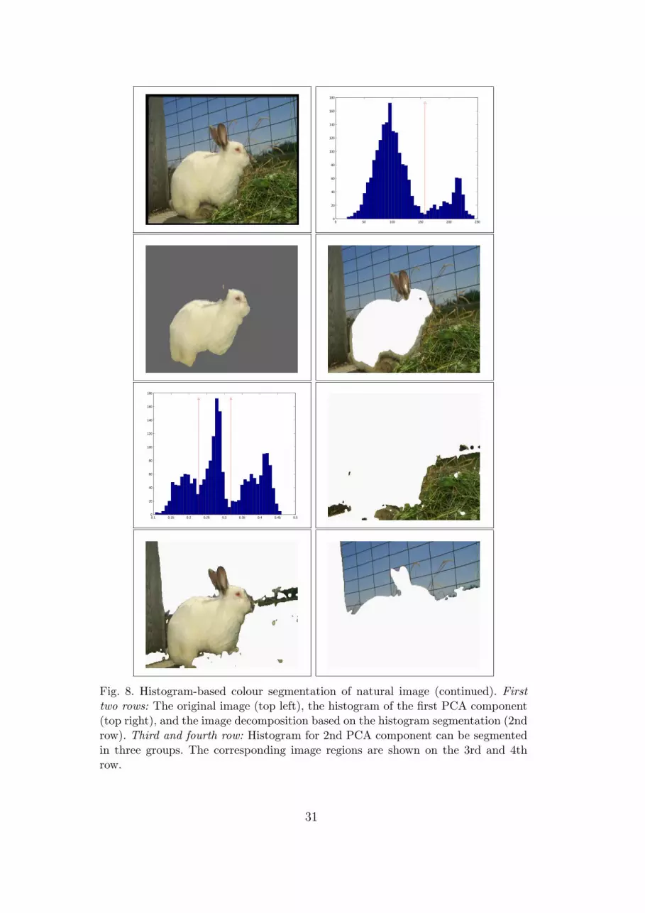
Fig. 8. Histogram-based colour segmentation of natural image (continued). Firsttwo rows: The original image (top left), the histogram of the first PCA component(top right), and the image decomposition based on the histogram segmentation (2ndrow). Third and fourth row: Histogram for 2nd PCA component can be segmentedin three groups. The corresponding image regions are shown on the 3rd and 4throw.

31

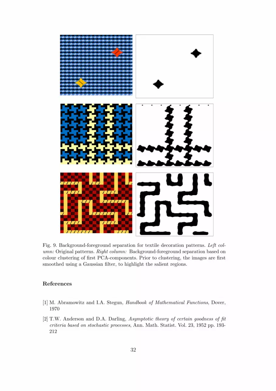
Fig. 9. Background-foreground separation for textile decoration patterns. Left col-umn: Original patterns. Right column: Background-foreground separation based oncolour clustering of first PCA-components. Prior to clustering, the images are firstsmoothed using a Gaussian filter, to highlight the salient regions.

References

[1] M. Abramowitz and I.A. Stegun, Handbook of Mathematical Functions, Dover,1970

[2] T.W. Anderson and D.A. Darling, Asymptotic theory of certain goodness of fitcriteria based on stochastic processes, Ann. Math. Statist. Vol. 23, 1952 pp. 193-212

32

[3] J.C. Bezdek, J. Keller, R. Krisnapuram, N.R. Pal: ”Fuzzy Models and Algorithmsfor Pattern Recognition in Image Processing”, Kluwer Academic Publishers,1999.

[4] C. de Boor, A Practical Guide to Splines. Applied Mathematical Sciences Vol.27, Springer-Verlag 1978

[5] A.P. Dempster, N.M. Laird and D.R. Rubin. Maximum likelihood fromincomplete data via the EM algorithm. J. Royal Statistical Soc. Ser. B. 39:1-38, 1977.

[6] R.O. Duda, P.E. Hart and D.G. Stork. Pattern Classification. WileyInterscience.Wiley and Sons, 2001.

[7] J. Durbin, Distribution Theory for Tests Based on the Sample DistributionFunction. SIAM Regional Conf. Series in Applied Mathematics, Society forindustrial and applied mathematics Philadelphia 1973

[8] R.L. Eubank: Spline Smoothing and Nonparametric Regression. Statistics:textbooks and monographs Vol. 90, Dekker New York 1988

[9] G. Frederix, E.J. Pauwels “A Statistically Principled Approach to HistogramSegmentation” CWI Report PNA-E0401 (2004), ISSN 1386-3711.

[10] T. Hastie, R. Tibshirani, J. Friedman: The Elements of Statistical Learning.Springer, 2001.

[11] A.K. Jain, M.N. Murty, P.J. Flynn ”Data Clustering: A Review”, ACMComputing Surveys, Vol. 31, No. 3, Sept 1999, pp. 264-323.

[12] K. Jajuga, A. Sokolowski and H. Bock, ”Classification, Clustering and DataAnalysis”, IFCS Conference Poland, Springer, 2002.

[13] L. Kaufman and P.J. Rousseeuw, ”Finding Groups in Data: An Introductionto Cluster Analysis”, J. Wiley and Sons, 1990.

[14] E.J. Pauwels and G. Frederix, ”Finding Salient Regions in Images ”, ComputerVision and Image Understanding, volume 75, number 1/2, July/August 1999,pp. 73-85.

[15] H. Schwetlick and V. Kunert, Spline smoothing under constraints on derivatives.Bit, Vol. 33, 1993 pp. 512-528

[16] G. Wahba: Spline Models for Observational Data. CBMS-NSF Regional Conf.Series in Applied Math. No 59, Society for Industrial and Applied Math.,Philadelphia 1990.

33