Embed Size (px)
Citation preview

by
http://ssrn.com/abstract=2139419
David Dillenberger, Juan Sebastián Lleras
Philipp Sadowski and Norio Takeoka
“A Theory of Subjective Learning”
PIER Working Paper 12-034
Penn Institute for Economic ResearchDepartment of Economics University of Pennsylvania
3718 Locust Walk Philadelphia, PA 19104-6297
[email protected] http://economics.sas.upenn.edu/pier
A Theory of Subjective Learning�
David Dillenbergery Juan Sebastián Llerasz
Philipp Sadowskix Norio Takeoka{
August 2012
Abstract
We study an individual who faces a dynamic decision problem in which the processof information arrival is unobserved by the analyst. We derive two utility representa-tions of preferences over menus of acts that capture the individual�s uncertainty abouthis future beliefs. The most general representation identi�es a unique probability dis-tribution over the set of posteriors that the decision maker might face at the timeof choosing from the menu. We use this representation to characterize a notion of�more preference for �exibility�via a subjective analogue of Blackwell�s (1951, 1953)comparisons of experiments. A more specialized representation uniquely identi�es in-formation as a partition of the state space. This result allows us to compare individualswho expect to learn di¤erently, even if they do not agree on their prior beliefs. Weconclude by extending the basic model to accommodate an individual who expects tolearn gradually over time by means of a subjective �ltration.Key words: Subjective learning, partitional learning, preference for �exibility, res-
olution of uncertainty, valuing more binary bets, subjective �ltration.
1. Introduction
1.1. Motivation and overview
The study of dynamic models of decision making under uncertainty when a �ow of informa-
tion on future risks is expected over time is central in all �elds of economics. For example,
investors decide when to invest and how much to invest based on what they expect to learn
�This paper extends, combines, and supersedes the working papers by Takeoka, N. (2005), and Lleras, J.S. (2011). The analysis in Section 2.2 previously appeared in Dillenberger, D. and Sadowski, P. (2012b).We thank David Ahn, Brendan Daley, Henrique de Olivera , Larry Epstein, Kazuya Hyogo, Atsushi Kajii,Shachar Kariv, Peter Landry, Jian Li, Atsushi Nishimura, Wolfgang Pesendorfer, Todd Sarver, and ChrisShannon for useful comments and suggestions.
yDepartment of Economics, University of Pennsylvania. E-mail: [email protected] of Social and Decision Sciences, CMU. E-mail: [email protected] of Economics, Duke University. E-mail: [email protected]{Department of Economics, Yokohama National University. E-mail: [email protected]
1

about the distribution of future cash �ows. The concepts of value of information and value of
�exibility (option value) quantify the positive e¤ects of relying on more precise information
structures.1
A standard dynamic decision problem has three components: the �rst component is a
set of states of the world that capture all relevant aspects of the decision environment. The
second component is a set of feasible intermediate actions, each of which determines the
payo¤ for any realized state. The third component is a description of what the decision
maker expects to learn; this component is formalized as an information structure, which is
the set of possible signals about the states that are expected to arrive over time and the
joint distribution of signals and states.
In many situations, the analyst may be con�dent in his understanding of the relevant
state space and the relevant set of actions. He may, however, not be aware of the information
structure people perceive. People may have access to private data which is unforeseen by
others; they may interpret data in an idiosyncratic way; or they may be selective in the data
they observe, for example by focusing their attention on speci�c signals. We collectively
refer to those situations as �subjective learning�. A natural question is whether we can
rely on only the �rst two components above and infer an individual�s subjective information
structure solely from his observed choice behavior. If the answer is in the a¢ rmative, we
ask whether we can compare the behavior of individuals who perceive di¤erent information
structures and how such comparisons relate to the comparative statics for incremental in-
creases in informativeness when learning is objective. These questions will be the subject of
our analysis.
We consider an objective state space. Actions correspond to acts, that is, state-contingent
payo¤s, and preferences are de�ned over sets (or menus) of acts. The interpretation is that
the decision maker (henceforth DM) initially chooses among menus and subsequently chooses
an act from the menu. If the ultimate choice of an act takes place in the future, then the DM
may expect information to arrive prior to this choice. Analyzing today�s preferences over
future choice situations (menus of acts rather than the acts themselves) allows us to capture
the e¤ect of the information the DM expects to learn via his value for �exibility (having
more future options available). The preference relation over menus of acts is thus the only
primitive of the model, leaving the information structure that the DM faces, as well as his
ultimate choice of an act, unmodeled.2
Section 2 outlines the most general model that captures subjective learning. Theorem 1
1For a comprehensive survey of the theoretical literature, see Gollier (2001, chapters 24 and 25).2In particular, our approach does not require the analyst to collect data that corresponds to a state-
contingent random choice from menus.
2
derives a subjective-learning representation that can be interpreted as follows: the DM be-
haves as if he has beliefs over the possible posterior distributions over the state space that he
might face at the time of choosing from the menu. For each posterior, he expects to choose
from the menu the act that maximizes the corresponding expected utility. The model is
parameterized by a probability measure on the collection of all possible posterior distribu-
tions. This probability measure describes the DM�s subjective information structure and is
uniquely identi�ed from choice behavior. The axioms that are equivalent to the existence
of a subjective-learning representation are the familiar axioms of Ranking, vNM Continuity,
Nontriviality, and Independence, in addition to Dominance, which implies monotonicity in
payo¤s, and Set Monotonicity, which captures preference for �exibility.
Identi�cation enables us to compare di¤erent decision makers in terms of their preferences
for �exibility. We say that DM1 has more preference for �exibility than DM2 if whenever
DM1 prefers to commit to a particular action rather than to maintain multiple options, so
does DM2. Theorem 2 states that DM1 has more preference for �exibility than DM2 if
and only if DM1�s distribution of posterior beliefs is a mean-preserving spread of DM2�s.
This result is analogous to Blackwell�s (1951, 1953) comparisons of experiments (in terms
of their information content) in a domain where probabilities are objective and comparisons
are made with respect to the accuracy of information structures. To rephrase our result in
the language of Blackwell, DM1 has more preference for �exibility than DM2 if and only if
DM2 would be weakly better o¤ if he could rely on the information structure induced by the
subjective beliefs of DM1.
A subjective-learning representation does not allow the identi�cation of information in-
dependently of the induced changes in beliefs. The reason is that the signals do not have
an objective meaning, that is, they do not correspond to events in the state space. Section
3 addresses this issue by studying the behavioral implications of a (subjective) partitional
information structure. A partition of the state space is a canonical formalization of infor-
mation that describes signals as events in the state space.3 This formalization is empirically
meaningful: an outside observer who knows the state of the world will also know the in-
formation that the decision maker will receive. Theorem 3 derives a partitional-learning
representation that can be interpreted as follows: the DM has in mind a partition of the
state space and prior beliefs over the individual states. The partition describes what he ex-
pects to learn before facing the choice of an alternative from the menu. The DM�s posterior
beliefs conditional on learning an event in the partition are fully determined from the prior
3For example, it is standard to model information as a partition of the state space in the literature ongames with incomplete information, that originated in the seminal contributions of Harsanyi (1967) andAumann (1976).
3

beliefs using Bayes�law. For each event, the DM plans to choose an act that maximizes the
corresponding expected utility. The partition and the beliefs are endogenous components
of the model, which are uniquely identi�ed from choice behavior. Given the assumptions of
Theorem 1, Theorem 3 requires only one additional axiom, Contingent Planning. Suppose
the DM anticipates receiving deterministic signals, that is, given the (unknown) true state
of the world, he knows what information he will learn. In this case, he is sure about the
act he will choose from the menu, contingent on the true state. The DM is thus indi¤erent
between choosing from the menu after learning the deterministic signal, and committing,
for every state, to receive the payo¤ his certain choice would have generated in that state.
Axiom Contingent Planning captures this indi¤erence.
Individuals who disagree on their prior beliefs are not comparable in terms of their pref-
erence for �exibility. A partitional-learning representation facilitates the behavioral com-
parisons of such individuals, because partitions can be partially ranked in terms of their
�neness, independently of any prior beliefs. The behavior of two individuals who expect to
receive di¤erent information di¤ers in the value they derive from the availability of binary
bets. Suppose the DM prefers committing to a constant act that pays c regardless of the
state over committing to an act that o¤ers a binary bet on state s versus state s0 (in the
sense that it pays well on s, pays badly on s0, and pays c otherwise). It may still be the case
that the DM values the binary bet as an option that is available in addition to c. We say
that DM1 values more binary bets than DM2 if for any two states s and s0 and payo¤ c for
which the premise above holds, whenever DM1 does not value the binary bet as an option in
addition to c, neither does DM2. Theorem 4 states that DM1 values more binary bets than
DM2 if and only if he expects to receive more information than DM2, in the sense that his
partition is �ner.4
We conclude by extending the basic model to accommodate a DM who expects to learn
gradually over time. Suppose that the DM can choose among pairs of the form (F; t), where
F is a menu and t is the time by which an alternative from the menu must be chosen. Suppose
that �xing t, DM�s preferences satisfy all the postulates underlying the partitional-learning
representation. Furthermore, suppose that the DM prefers to delay his choice from any menu
F , in the sense that (F; t) is weakly preferred to (F; t0) if t > t0, and he is indi¤erent to the
timing if F is a singleton (since then the future choice is trivial). Under these assumptions,
the DM has more preference for �exibility at time t than at t0, which means, by Theorem 4,
that the partition at time t must be �ner than that at t0. Using this observation, we provide
4An additional requirement for this comparison is that the two DMs agree on whether or not payo¤s instate s are valuable at all. This implies that while their prior beliefs need not be the same, they shouldhave the same support. If, in addition, their prior beliefs are the same, then DM1 has more preference for�exibility than DM2.
4
a learning by �ltration representation, which suggests that the DM behaves as if he has in
mind a �ltration indexed by continuous time. Both the �ltration, which is the timing of
information arrival with the sequence of partitions it induces, and the DM�s prior beliefs are
uniquely determined from choice behavior.
1.2. Related literature
To our knowledge, very few papers have explored the idea of subjective learning. Dillen-
berger and Sadowski (2012a) use the same domain as in the present paper to study the
most general representation for which signals correspond to events and the DM is Bayesian.
They characterize the class of information structures that admit such a representation as a
generalization of a set partition, which does not require deterministic signals (that is, the
true state of the world may appear in more than one event). Dillenberger and Sadowski show
that the generalized-partition model can be applied to study an individual who anticipates
gradual resolution of uncertainty over time, without extending the domain as we do in Sec-
tion 4. Takeoka (2007) uses a di¤erent approach to study subjective temporal resolution of
uncertainty. He analyzes choice between what one might term �compound menus�(menus
over menus etc.) Hyogo (2007) derives a representation that features beliefs over posteriors
on a richer domain, where the DM simultaneously chooses a menu of acts and takes an action
that might in�uence the (subjective) process of information arrival.
More generally, our work is part of the preferences over menus literature initiated by
Kreps (1979). Most papers in this literature study uncertainty over future tastes, and not
over beliefs on an objective state space. Kreps (1979) studies preferences over menus of
deterministic alternatives. Dekel, Lipman, and Rustichini (2001) extend Kreps�domain of
choice to menus of lotteries. The �rst �ve axioms in Section 2.1 are adapted from Dekel
et al.�s paper. Our proof of the corresponding theorem relies on a sequence of geometric
arguments that establish the close connection between our domain and theirs. In the set-
ting of preferences over menus of lotteries, Ergin and Sarver (2010) provide an alternative
to Hyogo�s (2007) approach of modeling costly information acquisition. Recently, De Oliv-
era (2012) and Mihm and Ozbek (2012) combine the framework of the present paper with
Ergin and Sarver�s idea of costly contemplation to give behavioral foundations to rational
inattention.
2. A general model of subjective learning
Let S = fs1; :::; skg be a �nite state space. An act is a mapping f : S ! [0; 1]. Let F be
the set of all acts. Let K (F) be the set of all non-empty compact subsets of F . Capital
5

letters denote sets, or menus, and small letters denote acts. For example, a typical menu is
F = ff; g; h; :::g 2 K (F). The space K (F) is endowed with the Hausdor¤ topology.5 Weinterpret payo¤s in [0; 1] to be in utils; that is, we assume that the cardinal utility function
over outcomes is known and payo¤s are stated in its units. An alternative interpretation is
that there are two monetary prizes x > y, and f (s) = ps (x) 2 [0; 1] is the probability ofgetting the greater prize in state s.6
Let � be a binary relation over K (F). The symmetric and asymmetric components of� are denoted by � and �, respectively.
2.1. Axioms and representation result
We impose the following axioms on �:
Axiom 1 (Ranking). The relation � is a weak order.
De�nition 1. Let �F+(1� �)G := f�f + (1� �) g : f 2 F; g 2 Gg, where �f+(1� �) gis the act that yields �f (s) + (1� �) g (s) in state s.
Axiom 2 (vNM Continuity). If F � G � H then there are �; � 2 (0; 1), such that
�F + (1� �)H � G � �F + (1� �)H.
Axiom 3 (Nontriviality). There are F and G such that F � G:
The �rst three axioms play the same role here as they do in more familiar contexts.
Axiom 4 (Independence). For all F; G; H, and � 2 [0; 1],
F � G, �F + (1� �)H � �G+ (1� �)H:
In the domain of menus of acts, Axiom 4 implies that the DM�s preferences must be linear
in payo¤s. This is plausible since we interpret payo¤s in [0; 1] directly as utils, as discussed
above.5Identify F with the unit cube [0; 1]jSj and let d denote the Euclidean metric. Then dh (F;G), the
Hausdor¤ distance between F and G, is de�ned by
dh (F;G) = max
(supf2F
infg2G
d (f; g) ; supf2G
infg2F
d (f; g)
):
6Our analysis can be easily extended to the case where, instead of [0; 1], the range of acts is a moregeneral vector space. In particular, it could be formulated in the Anscombe and Aumann (1963) setting.Since our focus is on deriving the DM�s subjective information structure, we abstract from deriving theutility function (which is a standard exercise) by looking directly at utility acts instead of the correspondingAnscombe-Aumann acts.
6
Axiom 5 (Set monotonicity). If F � G then G � F .
Axiom 5 was �rst proposed in Kreps (1979). It captures preference for �exibility, that is,
bigger sets are weakly preferred.
The interpretation of f (�) as a vector of utils requires the following payo¤-monotonicityaxiom.
Axiom 6 (Domination). If f � g and f 2 F then F � F [ fgg.
Axioms 1-6 are necessary and su¢ cient for the most general representation of subjective
learning.
De�nition 2. The binary relation � has a subjective-learning representation if thereis a probability measure p on �(S), the space of all probability measures on S, such that
the function V : K (F)! R given by
V (F ) =R
�(S)
maxf2F
�Ps2Sf (s)� (s)
�dp (�)
represents �.
Theorem 1. The relation � satis�es Axioms 1�6 if and only if it has a subjective-learningrepresentation. Furthermore, the probability measure p is unique.
Proof. See Appendix 5.1.The representation in Theorem 1 suggests that the DM is uncertain about which posterior
beliefs � he will have at the time he makes a choice from the menu. This uncertainty
is captured by the information structure p, which is a distribution over posterior beliefs.
Theorem 1 spells out the conditions under which preferences over menus of acts can be
rationalized as emerging from this notion of subjective learning. The notion is not restrictive,
in the sense that only one of the axioms, Axiom 5, has the �avor of expected information
arrival; the DM likes bigger sets since more available options allow him to better adjust his
choice to his updated beliefs.
Dekel, Lipman, and Rustichini (2001, henceforth DLR) consider choice over menus of
objective lotteries. They provide a representation that suggests that the DM is uncertain
about the taste he will face at the time he chooses from the menu (a relevant corrigendum is
Dekel, Lipman, Rustichini, and Sarver (2007)). Our proof of Theorem 1 relies on a sequence
of geometric arguments that establish the close connection between our domain and theirs,
as we now explain.
7
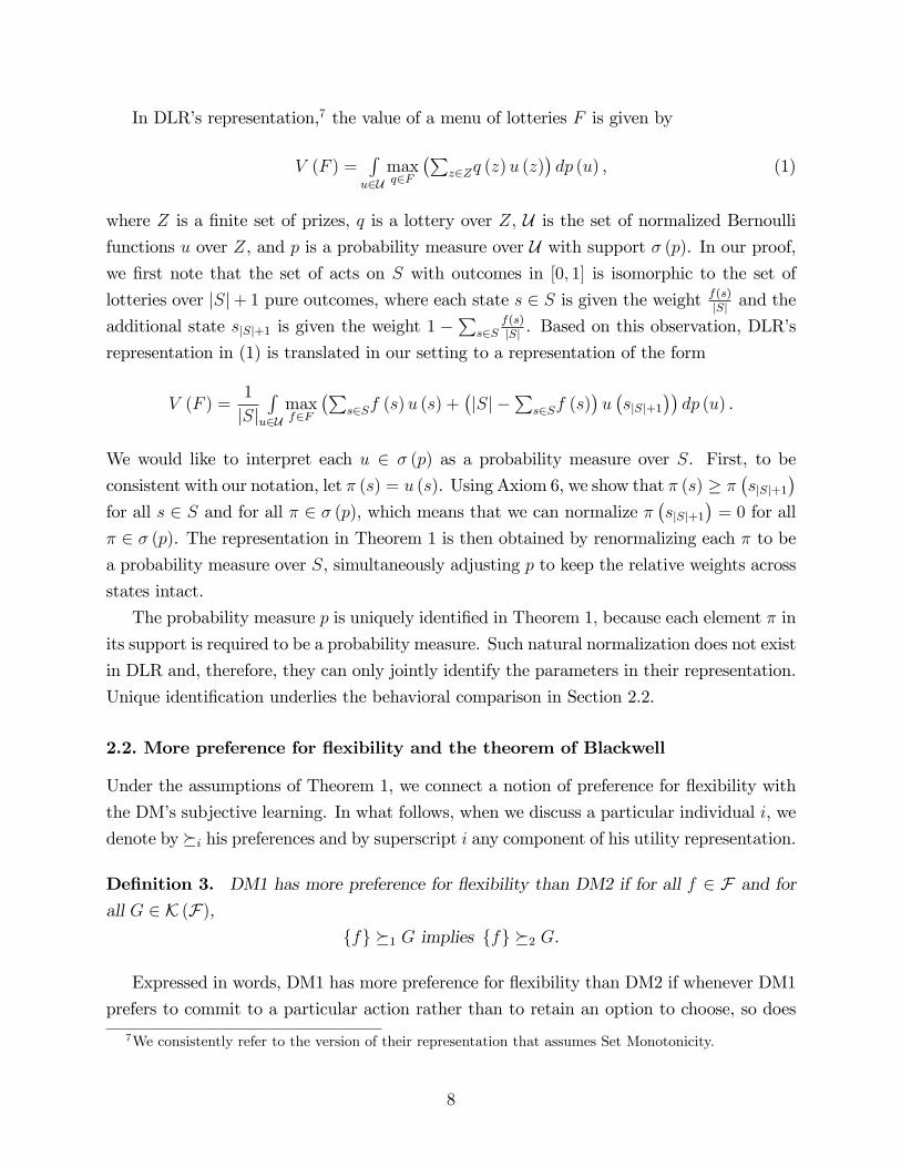
In DLR�s representation,7 the value of a menu of lotteries F is given by
V (F ) =Ru2Umaxq2F
�Pz2Zq (z)u (z)
�dp (u) , (1)
where Z is a �nite set of prizes, q is a lottery over Z, U is the set of normalized Bernoullifunctions u over Z, and p is a probability measure over U with support � (p). In our proof,we �rst note that the set of acts on S with outcomes in [0; 1] is isomorphic to the set of
lotteries over jSj+ 1 pure outcomes, where each state s 2 S is given the weight f(s)jSj and the
additional state sjSj+1 is given the weight 1 �P
s2Sf(s)jSj . Based on this observation, DLR�s
representation in (1) is translated in our setting to a representation of the form
V (F ) =1
jSjRu2Umaxf2F
�Ps2Sf (s)u (s) +
�jSj �
Ps2Sf (s)
�u�sjSj+1
��dp (u) .
We would like to interpret each u 2 � (p) as a probability measure over S. First, to beconsistent with our notation, let � (s) = u (s). Using Axiom 6, we show that � (s) � �
�sjSj+1
�for all s 2 S and for all � 2 � (p), which means that we can normalize �
�sjSj+1
�= 0 for all
� 2 � (p). The representation in Theorem 1 is then obtained by renormalizing each � to be
a probability measure over S, simultaneously adjusting p to keep the relative weights across
states intact.
The probability measure p is uniquely identi�ed in Theorem 1, because each element � in
its support is required to be a probability measure. Such natural normalization does not exist
in DLR and, therefore, they can only jointly identify the parameters in their representation.
Unique identi�cation underlies the behavioral comparison in Section 2.2.
2.2. More preference for �exibility and the theorem of Blackwell
Under the assumptions of Theorem 1, we connect a notion of preference for �exibility with
the DM�s subjective learning. In what follows, when we discuss a particular individual i, we
denote by �i his preferences and by superscript i any component of his utility representation.
De�nition 3. DM1 has more preference for �exibility than DM2 if for all f 2 F and for
all G 2 K (F),ffg �1 G implies ffg �2 G.
Expressed in words, DM1 has more preference for �exibility than DM2 if whenever DM1
prefers to commit to a particular action rather than to retain an option to choose, so does
7We consistently refer to the version of their representation that assumes Set Monotonicity.
8
DM2.8 ;9
The next claim shows that two DMs who are comparable in terms of their preference for
�exibility must agree on the ranking of singletons.
Claim 1. Suppose DM1 has more preference for �exibility than DM2. Then
ffg �1 fgg if and only if ffg �2 fgg :
Proof. See Appendix 5.2.We now compare subjective information structures in analogy to the notion of better
information proposed by Blackwell (1951, 1953) in the context of objective information.
De�nition 4 below says that an information structure is better than another one if and only if
both structures induce the same prior probability distribution, and all posterior probabilities
of the latter are a convex combination of the posterior probabilities of the former.
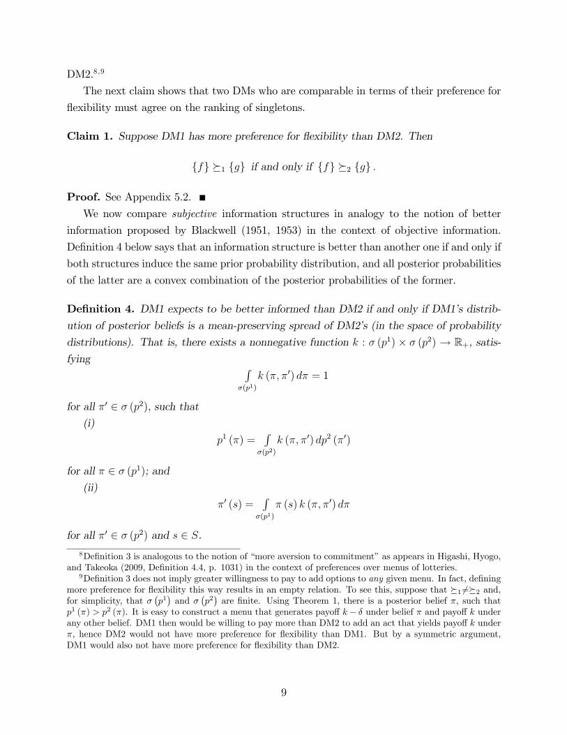
De�nition 4. DM1 expects to be better informed than DM2 if and only if DM1�s distrib-ution of posterior beliefs is a mean-preserving spread of DM2�s (in the space of probability
distributions). That is, there exists a nonnegative function k : � (p1) � � (p2) ! R+, satis-fying R
�(p1)
k (�; �0) d� = 1
for all �0 2 � (p2), such that(i)
p1 (�) =R
�(p2)
k (�; �0) dp2 (�0)
for all � 2 � (p1); and(ii)
�0 (s) =R
�(p1)
� (s) k (�; �0) d�
for all �0 2 � (p2) and s 2 S.8De�nition 3 is analogous to the notion of �more aversion to commitment�as appears in Higashi, Hyogo,
and Takeoka (2009, De�nition 4.4, p. 1031) in the context of preferences over menus of lotteries.9De�nition 3 does not imply greater willingness to pay to add options to any given menu. In fact, de�ning
more preference for �exibility this way results in an empty relation. To see this, suppose that �1 6=�2 and,for simplicity, that �
�p1�and �
�p2�are �nite. Using Theorem 1, there is a posterior belief �, such that
p1 (�) > p2 (�). It is easy to construct a menu that generates payo¤ k� � under belief � and payo¤ k underany other belief. DM1 then would be willing to pay more than DM2 to add an act that yields payo¤ k under�, hence DM2 would not have more preference for �exibility than DM1. But by a symmetric argument,DM1 would also not have more preference for �exibility than DM2.
9
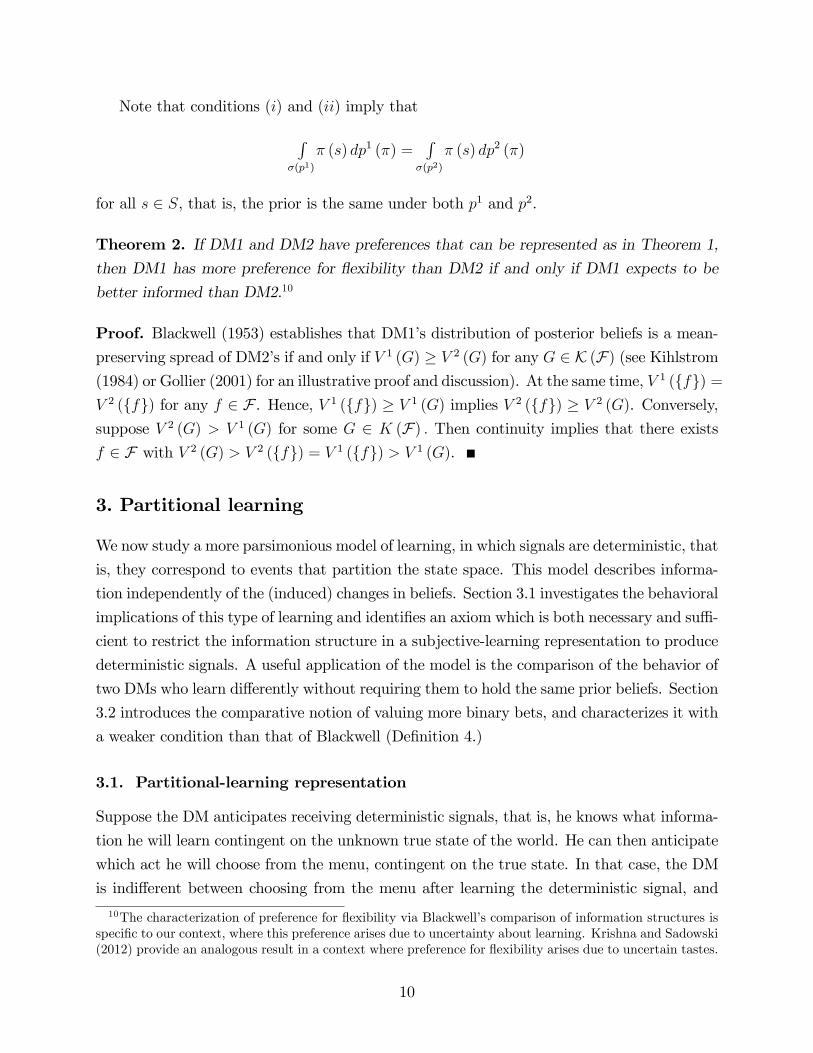
Note that conditions (i) and (ii) imply that
R�(p1)
� (s) dp1 (�) =R
�(p2)
� (s) dp2 (�)
for all s 2 S, that is, the prior is the same under both p1 and p2.
Theorem 2. If DM1 and DM2 have preferences that can be represented as in Theorem 1,
then DM1 has more preference for �exibility than DM2 if and only if DM1 expects to be
better informed than DM2.10
Proof. Blackwell (1953) establishes that DM1�s distribution of posterior beliefs is a mean-preserving spread of DM2�s if and only if V 1 (G) � V 2 (G) for any G 2 K (F) (see Kihlstrom(1984) or Gollier (2001) for an illustrative proof and discussion). At the same time, V 1 (ffg) =V 2 (ffg) for any f 2 F . Hence, V 1 (ffg) � V 1 (G) implies V 2 (ffg) � V 2 (G). Conversely,suppose V 2 (G) > V 1 (G) for some G 2 K (F) : Then continuity implies that there existsf 2 F with V 2 (G) > V 2 (ffg) = V 1 (ffg) > V 1 (G).
3. Partitional learning
We now study a more parsimonious model of learning, in which signals are deterministic, that
is, they correspond to events that partition the state space. This model describes informa-
tion independently of the (induced) changes in beliefs. Section 3.1 investigates the behavioral
implications of this type of learning and identi�es an axiom which is both necessary and su¢ -
cient to restrict the information structure in a subjective-learning representation to produce
deterministic signals. A useful application of the model is the comparison of the behavior of
two DMs who learn di¤erently without requiring them to hold the same prior beliefs. Section
3.2 introduces the comparative notion of valuing more binary bets, and characterizes it with
a weaker condition than that of Blackwell (De�nition 4.)
3.1. Partitional-learning representation
Suppose the DM anticipates receiving deterministic signals, that is, he knows what informa-
tion he will learn contingent on the unknown true state of the world. He can then anticipate
which act he will choose from the menu, contingent on the true state. In that case, the DM
is indi¤erent between choosing from the menu after learning the deterministic signal, and
10The characterization of preference for �exibility via Blackwell�s comparison of information structures isspeci�c to our context, where this preference arises due to uncertainty about learning. Krishna and Sadowski(2012) provide an analogous result in a context where preference for �exibility arises due to uncertain tastes.
10
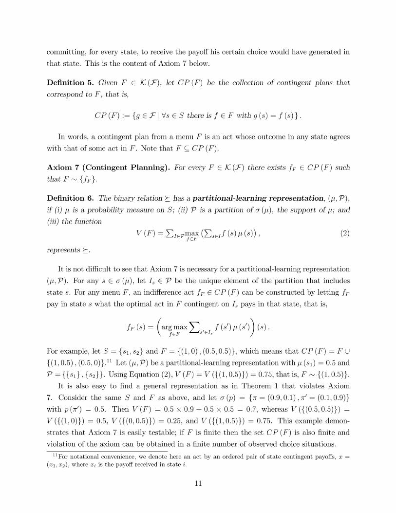
committing, for every state, to receive the payo¤ his certain choice would have generated in
that state. This is the content of Axiom 7 below.
De�nition 5. Given F 2 K (F), let CP (F ) be the collection of contingent plans thatcorrespond to F , that is,
CP (F ) := fg 2 F j 8s 2 S there is f 2 F with g (s) = f (s)g :
In words, a contingent plan from a menu F is an act whose outcome in any state agrees
with that of some act in F . Note that F � CP (F ).
Axiom 7 (Contingent Planning). For every F 2 K (F) there exists fF 2 CP (F ) suchthat F � ffFg.
De�nition 6. The binary relation � has a partitional-learning representation, (�;P),if (i) � is a probability measure on S; (ii) P is a partition of � (�), the support of �; and
(iii) the function
V (F ) =P
I2Pmaxf2F
�Ps2If (s)� (s)
�, (2)
represents �.
It is not di¢ cult to see that Axiom 7 is necessary for a partitional-learning representation
(�;P). For any s 2 � (�), let Is 2 P be the unique element of the partition that includes
state s. For any menu F , an indi¤erence act fF 2 CP (F ) can be constructed by letting fFpay in state s what the optimal act in F contingent on Is pays in that state, that is,
fF (s) =
�argmaxf2F
Xs02Is
f (s0)� (s0)
�(s) :
For example, let S = fs1; s2g and F = f(1; 0) ; (0:5; 0:5)g, which means that CP (F ) = F [f(1; 0:5) ; (0:5; 0)g.11 Let (�;P) be a partitional-learning representation with � (s1) = 0:5 andP = ffs1g ; fs2gg. Using Equation (2), V (F ) = V (f(1; 0:5)g) = 0:75, that is, F � f(1; 0:5)g.It is also easy to �nd a general representation as in Theorem 1 that violates Axiom
7. Consider the same S and F as above, and let � (p) = f� = (0:9; 0:1) ; �0 = (0:1; 0:9)gwith p (�0) = 0:5. Then V (F ) = 0:5 � 0:9 + 0:5 � 0:5 = 0:7, whereas V (f(0:5; 0:5)g) =V (f(1; 0)g) = 0:5, V (f(0; 0:5)g) = 0:25, and V (f(1; 0:5)g) = 0:75. This example demon-
strates that Axiom 7 is easily testable; if F is �nite then the set CP (F ) is also �nite and
violation of the axiom can be obtained in a �nite number of observed choice situations.11For notational convenience, we denote here an act by an ordered pair of state contingent payo¤s, x =
(x1; x2), where xi is the payo¤ received in state i.
11
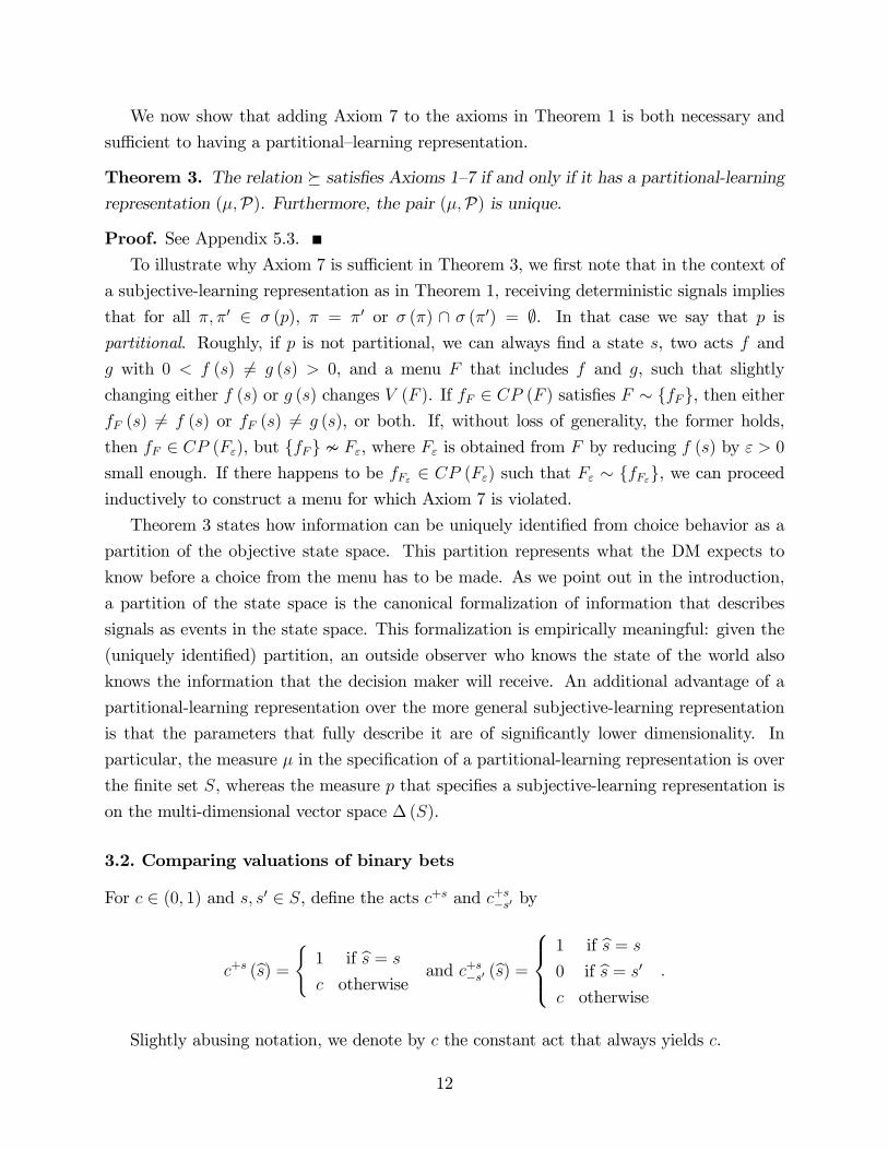
We now show that adding Axiom 7 to the axioms in Theorem 1 is both necessary and
su¢ cient to having a partitional�learning representation.
Theorem 3. The relation � satis�es Axioms 1�7 if and only if it has a partitional-learningrepresentation (�;P). Furthermore, the pair (�;P) is unique.
Proof. See Appendix 5.3.To illustrate why Axiom 7 is su¢ cient in Theorem 3, we �rst note that in the context of
a subjective-learning representation as in Theorem 1, receiving deterministic signals implies
that for all �; �0 2 � (p), � = �0 or � (�) \ � (�0) = ;. In that case we say that p is
partitional. Roughly, if p is not partitional, we can always �nd a state s, two acts f and
g with 0 < f (s) 6= g (s) > 0, and a menu F that includes f and g, such that slightly
changing either f (s) or g (s) changes V (F ). If fF 2 CP (F ) satis�es F � ffFg, then eitherfF (s) 6= f (s) or fF (s) 6= g (s), or both. If, without loss of generality, the former holds,
then fF 2 CP (F"), but ffFg � F", where F" is obtained from F by reducing f (s) by " > 0
small enough. If there happens to be fF" 2 CP (F") such that F" � ffF"g, we can proceedinductively to construct a menu for which Axiom 7 is violated.
Theorem 3 states how information can be uniquely identi�ed from choice behavior as a
partition of the objective state space. This partition represents what the DM expects to
know before a choice from the menu has to be made. As we point out in the introduction,
a partition of the state space is the canonical formalization of information that describes
signals as events in the state space. This formalization is empirically meaningful: given the
(uniquely identi�ed) partition, an outside observer who knows the state of the world also
knows the information that the decision maker will receive. An additional advantage of a
partitional-learning representation over the more general subjective-learning representation
is that the parameters that fully describe it are of signi�cantly lower dimensionality. In
particular, the measure � in the speci�cation of a partitional-learning representation is over
the �nite set S, whereas the measure p that speci�es a subjective-learning representation is
on the multi-dimensional vector space �(S).
3.2. Comparing valuations of binary bets
For c 2 (0; 1) and s; s0 2 S, de�ne the acts c+s and c+s�s0 by
c+s (bs) = ( 1 if bs = sc otherwise
and c+s�s0 (bs) =8><>:1 if bs = s0 if bs = s0c otherwise
:
Slightly abusing notation, we denote by c the constant act that always yields c.
12

De�nition 7. DM1 values more binary bets than DM2 if for all s; s0 2 S and c 2 (0; 1),(i) fcg �1 fc+sg , fcg �2 fc+sg; and(ii) fcg �i
�c+s�s0
for i = 1; 2 and fcg �1
�c+s�s0 ; c
) fcg �2
�c+s�s0 ; c
.
Condition (i) says that the two DMs agree on whether or not payo¤s in state s are valu-
able. Condition (ii) says that having the bet c+s�s0 available is valuable to DM1 whenever it is
valuable to DM2. The notion of valuing more binary bets weakens the notion of more pref-
erence for �exibility (De�nition 3); Condition (ii) is implied by De�nition 3 and Condition
(i) is implied by Claim 1.
A natural measure of the amount of information that a DM expects to receive is the
�neness of his partition.
De�nition 8. The partition P is �ner than Q if for every I 2 P there is I 0 2 Q such that
I � I 0.
Theorem 4. If DM1 and DM2 have preferences that can be represented as in Theorem 3,
then
(i) DM1 values more binary bets than DM2 if and only if � (�1) = � (�2) and P1 is �nerthan P2.(ii) DM1 has more preference for �exibility than DM2, if and only if �1 = �2 and P1 is
�ner than P2.
Proof. See Appendix 5.4.Theorem 4 (i) compares the behavior of two individuals who expect to learn di¤erently,
without requiring that they share the same prior beliefs; instead, the only requirement is
that their prior beliefs have the same support. For example, DM1 might consider himself
a better experimenter than DM2, in the sense of expecting a �ner partition, even though
DM2�s prior is sharper. In contrast, and in line with Theorem 2, Theorem 4 (ii) states that
the stronger comparison of more preference for �exibility corresponds exactly to adding the
requirement that the prior beliefs are the same.
4. Subjective gradual resolution of uncertainty
We conclude by extending the model outlined in the previous sections to accommodate a
DM who expects to learn gradually over time. Suppose that the DM can choose not only
among menus but also the future time by which he will make his choice of an act from the
menu. Formally, consider the domain K (F)� [0; 1], where a typical element (F; t) representsa menu and a time by which an alternative from the menu must be chosen.
13

Let �� be a preference relation over K (F)� [0; 1]. For each t 2 [0; 1], de�ne the inducedbinary relation ��t by G ��t F , (G; t) �� (F; t). Clearly ��t is a preference relation (itsatis�es Axiom 1). We assume that each ��t also satis�es Axioms 2�6 and hence admits asubjective-learning representation, that is,
Vt (F ) =R
�(S)
maxf2F
�Ps2Sf (s)� (s)
�dpt (�)
represents ��t , and pt (�) is unique.For each F 2 K (F), de�ne the induced binary relation ��F by t ��F t0 , (F; t) �� (F; t0).
Again, ��F satis�es Axiom 1. We impose on ��F the following additional axioms:
Axiom 8 (Preference for choosing late). For all t; t0 2 [0; 1] and F 2 K (F),
t ��F t0 , t � t0:
If the DM expects uncertainty to resolve over time, then waiting enables him to make a
more informed choice from the menu. The next axiom rules out intrinsic preference for the
timing of choice, independently of the instrumental value of information.
Axiom 9 (Time-independent singleton preferences). For all t; t0 2 [0; 1] and f 2 F ,
t ��ffg t0:
Since the singleton menu ffg does not leave the DM any �exibility to adjust his choice
to new information, the time component should play no role in its evaluation.
De�nition 9. The collection of measures (pt)t2[0;1] is a gradual-learning representationif the function V � given by
V � (F; t) =R
�(S)
maxf2F
�Ps2Sf (s)� (s)
�dpt (�)
represents ��, and pt is a mean preserving spread of pt0, whenever t � t0:
Theorem 5. Let �� be a preference relation over F� [0; 1]. The following two statementsare equivalent:
(i) For each t 2 [0; 1], the relation ��t satis�es Axioms 2�6, and for each F 2 K (F), therelation ��F satis�es Axiom 8 and Axiom 9.
(ii) The relation �� has a gradual-learning representation. Furthermore, the collection(pt)t2[0;1] is unique.
14
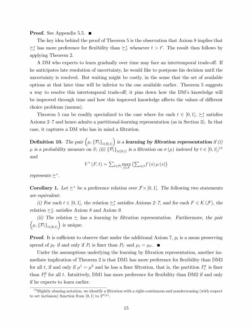
Proof. See Appendix 5.5.The key idea behind the proof of Theorem 5 is the observation that Axiom 8 implies that
��t has more preference for �exibility than ��t0 whenever t > t0. The result then follows byapplying Theorem 2.
A DM who expects to learn gradually over time may face an intertemporal trade-o¤. If
he anticipates late resolution of uncertainty, he would like to postpone his decision until the
uncertainty is resolved. But waiting might be costly, in the sense that the set of available
options at that later time will be inferior to the one available earlier. Theorem 5 suggests
a way to resolve this intertemporal trade-o¤; it pins down how the DM�s knowledge will
be improved through time and how this improved knowledge a¤ects the values of di¤erent
choice problems (menus).
Theorem 5 can be readily specialized to the case where for each t 2 [0; 1], ��t satis�esAxioms 2�7 and hence admits a partitional-learning representation (as in Section 3). In that
case, it captures a DM who has in mind a �ltration.
De�nition 10. The pair��; fPtgt2[0;1]
�is a learning by �ltration representation if (i)
� is a probability measure on S; (ii) fPtgt2[0;1] is a �ltration on � (�) indexed by t 2 [0; 1];12
and
V � (F; t) =P
I2Ptmaxf2F
�Ps2If (s)� (s)
�represents ��.
Corollary 1. Let �� be a preference relation over F� [0; 1]. The following two statementsare equivalent:
(i) For each t 2 [0; 1], the relation ��t satis�es Axioms 2�7, and for each F 2 K (F), therelation ��F satis�es Axiom 8 and Axiom 9.
(ii) The relation � has a learning by �ltration representation. Furthermore, the pair��; fPtgt2[0;1]
�is unique.
Proof. It is su¢ cient to observe that under the additional Axiom 7, pt is a mean preservingspread of pt0 if and only if Pt is �ner than Pt0 and �t = �t0.
Under the assumptions underlying the learning by �ltration representation, another im-
mediate implication of Theorem 2 is that DM1 has more preference for �exibility than DM2
for all t, if and only if �1 = �2 and he has a �ner �ltration, that is, the partition P 1t is �ner
than P 2t for all t. Intuitively, DM1 has more preference for �exibility than DM2 if and only
if he expects to learn earlier.
12Slightly abusing notation, we identify a �ltration with a right-continuous and nondecreasing (with respectto set inclusion) function from [0; 1] to 2�(�).
15

5. Appendix
5.1. Proof of Theorem 1
It is easily veri�ed that any binary relation � with a subjective-learning representation
satis�es the axioms. We proceed to show the su¢ ciency of the axioms.
We can identify F with the set of all k�dimensional vectors, where each entry is in [0; 1].For reasons that will become clear below, we now introduce an arti�cial state, sk+1. Let
F 0 :=nf 0 2 [0; 1]k � [0; k]
���Pk+1i=1 f
0 (si) = ko:
Note that the k+ 1 component in f 0 equals k�Pk
i=1f0 (si). For f 0 2 F 0, denote by f 0k 2 F
the vector that agrees with the �rst k components of f 0. Since F and F 0 are isomorphic,
we can look at a preference relation on K (F 0), ��, de�ned by: F 0 �� G0 , F � G, whereF :=
�f 2 F
��f = f 0k for some f 0 2 F 0 and analogously for G.Claim 2. The relation �� satis�es the independence axiom.
Proof. Using the de�nition of �� and Axiom 4, we have, for all F 0; G0, and H 0 in K (F 0)
and for all � 2 [0; 1],
F 0 �� G0 , F � G, �F + (1� �)H � �G+ (1� �)H ,(�F + (1� �)H)0 �� (�G+ (1� �)H)0 , �F 0 + (1� �)H 0 �� �G0 + (1� �)H 0:
Let
F 00 :=nf 0 2 [0; k]k+1
���Pk+1i=1 f
0 (si) = ko:
Let F k+1 :=��
kk+1; :::; k
k+1
�2 K (F 0). Observe that for F 00 2 F 00 and " < 1
k2, "F 00 +
(1� ")F k+1 2 K (F 0). De�ne ��� on K (F 00) by F 00 ��� G00 , "F 00 + (1� ")F k+1 ��"G00 + (1� ")F k+1 for all " < 1
k2.
Claim 3. The relation ��� is the unique extension of �� to K (F 00) that satis�es the inde-
pendence axiom.
Proof. Note that the (k + 1)-dimensional vector�
kk+1; :::; k
k+1
�2 intF 0 � F 00, hence F k+1 �
intF 0 � F 00. We now show that ��� satis�es independence. For any F 00; G00; H 00 2 K (F 00)
16

and � 2 [0; 1],
F 00 ��� G00 , "F 00 + (1� ")F k+1 �� "G00 + (1� ")F k+1 ,��"F 00 + (1� ")F k+1
�+ (1� �)
�"H 00 + (1� ")F k+1
�= " (�F 00 + (1� �)H 00) + (1� ")F k+1 ����"G00 + (1� ")F k+1
�+ (1� �)
�"H 00 + (1� ")F k+1
�= " (�G00 + (1� �)H 00) + (1� ")F k+1 , �F 00 + (1� �)H 00 ��� �G00 + (1� �)H 00:
The �rst and third , is by the de�nition of ���. The second , is by Claim 2.13 This
argument shows that a linear extension exists. To show uniqueness, let b� be any linear
extension over K (F 00) of �. By independence, F 00 b� G00 , "F 00 + (1� ")F k+1 b� "G00 +
(1� ")F k+1. Since b� extends ��, they must agree on K (F 0). Therefore,
"F 00 + (1� ")F k+1 b� "G00 + (1� ")F k+1 , "F 00 + (1� ")F k+1 �� "G00 + (1� ")F k+1:
By combining the two equivalences above, we conclude that de�ning b� by F 00 b� G00 ,"F 00 + (1� ")F k+1 �� "G00 + (1� ")F k+1 is the only admissible extension of ��.The domain K (F 00) is formally equivalent to that of Dekel, Lipman, Rustichini, and
Sarver (2007, henceforth DLRS) with k+1 prizes. (The unit simplex is obtained by rescalingall elements of F 00 by 1=k, that is, by rede�ning F 00 as
nf 0 2 [0; 1]k+1 :
Pk+1i=1 f
0 (si) = 1o.)
Applying Theorem 2 in DLRS,14 one obtains the following representation of ���:
bV (F 00) = RM(S)
maxf 002F 00
�Ps2S[fsk+1gf
00 (s) b� (s)� dbp (b�) ;where M (S) :=
nb� ���Ps2S[fsk+1gb� (s) = 0 andPs2S[fsk+1g (b� (s))2 = 1o. Given the nor-malization of b� 2M (S), bp (�) is a unique probability measure. Note that bV also represents�� when restricted to its domain, K (F 0).
13The (=) sign in the third and in �fth lines are due to the fact that F k+1 is a singleton menu. For asingleton menu ffg and � 2 (0; 1) ;
� ffg+ (1� �) ffg = ffg
while, for example,
� ff; gg+ (1� �) ff; gg = ff; g; �f + (1� �) g; �g + (1� �) fg ;
is not generally equal to ff; gg :14DLRS provide a supplemental appendix which shows that, for the purpose of the theorem, their stronger
continuity assumption can be relaxed to the weaker notion of vNM continuity used in the present paper.
17

We aim for a representation of � of the form
V (F ) =R
�(S)
maxf2F
�Ps2Sf (s)� (s)
�dp (�) ,
where f (�) is a vector of utils and p (�) is a unique probability measure on �(S), the spaceof all probability measures on S.
We now explore the additional constraint imposed on bV by Axiom 6 and the de�nition
of ��.
Claim 4. b� (sk+1) � b� (s) for all s 2 S, bp�almost surely.Proof. Suppose there exists some event E �M (S) with bp (E) > 0 and b� (sk+1) > b� (s) forsome s 2 S and all b� 2 E: Let f 0 = (0; 0; :::; 0; "; 0; :::; k � ") ; where " is received in state sand k� " is received in state sk+1. Let g0 = (0; 0; ::0; 0; 0; :::; k). Then ff 0; g0g �� ff 0g. TakeF 0 = ff 0g (so that F 0 [ fg0g �� F 0). But note that Axiom 6 and the de�nition of �� implythat F 0 �� F 0 [ fg0g, which is a contradiction.Given our construction of bV , there are two natural normalizations that allow us to replace
the measure bp onM (S) with a unique probability measure p on �(S).
First, since sk+1 is an arti�cial state, the representation should satisfy � (sk+1) = 0,
p�almost surely. For all s 2 S and for all b�, de�ne � (b� (s)) := b� (s) � b� (sk+1). SincePk+1i=1 f
0 (si) = k and � simply adds a constant to every b�,argmaxf 002F 00
�Ps2S[fsk+1gf
00 (s) � (b� (s))� = argmaxf 002F 00
�Ps2S[fsk+1gf
00 (s) b� (s)�for all b� 2 � (bp). Furthermore, by Claim 4, � (b� (s)) � 0 for all s 2 S, bp�almost surely.Second, we would like to transform � � b� into a probability measure �. Let
� (s) := � (b� (s)) = �Ps02S� (b� (s0))� :(recall that � (b� (sk+1)) = 0). Since this transformation a¤ects the relative weight given toevent E � M (S) in the representation, we need p to be a probability measure on E that
o¤sets this e¤ect. The identi�cation result in DLRS implies that this p is unique and can be
calculated via the Radon-Nikodym derivative
dp (�)
dbp (b�) =P
s2S� (b� (s))RM(S)
�Ps2S� (b� (s))� dbp (b�) :
18

Therefore, � is represented by
V (F ) =R
�(S)
maxf2F
�Ps2Sf (s)� (s)
�dp (�) ;
and the measure p is unique.
5.2. Proof of Claim 1
Let G = fgg for some g 2 F . Applying De�nition 3 implies that if ffg �1 fgg thenffg �2 fgg. That is, any indi¤erence set of the restriction of �1 to singletons is a subset ofsome indi¤erence set of the restriction of �2 to singletons. The linearity (in probabilities)of the restriction of V i (�) to singletons implies that these indi¤erence sets are planes thatseparate any n�dimensional unit simplex, for n � (jSj � 1). Therefore, the indi¤erence setsof the restriction of �1 and �2 to singletons must coincide. Since the restrictions of �1 andof �2 to singletons share the same indi¤erence sets and since both relations are monotone,they must agree on all upper and lower contour sets. In particular, ffg �1 fgg if and onlyif ffg �2 fgg.
5.3. Proof of Theorem 3
First observe that any partitional-learning representation (�;P) (De�nition 6) can be writtenas a subjective-learning representation (De�nition 2), where the information structure p has
the property that � = �0 or � (�) \ � (�0) = ; for all �; �0 2 � (p). In this case we saythat p is partitional. If p is partitional, then for all s 2 S with
R�(S)
� (s) dp (�) > 0, the
prior probability � is de�ned by � (s) := p (�s)�s (s), where �s 2 �(S) denotes the uniqueposterior such that s 2 � (�s).For any F 2 K (F), let CP (F ) be the collection of contingent plans that correspond to
F , that is,
CP (F ) := fg 2 F j 8s 2 S there is f 2 F with g (s) = f (s)g :
Let ICP (F ) be the contingent plans that are indi¤erent to F ,
ICP (F ) := fg 2 CP (F ) j fgg � F g .
We now show that any partitional-learning representation satis�es Axiom 7.
Claim 5. If p is partitional, then for every F 2 K (F), ICP (F ) 6= ?:
19

Proof. Suppose that p is partitional. Using Theorem 1, for any set F we have
V (F ) =P
�maxf2F
(P
sf (s)� (s)) p (�)
=P
smaxf2F
(P
s0f (s0)�s (s
0)) ep (s) ;where ep is a probability distribution over S such that for all � 2 � (p),Ps2�(�)ep (s) = p (�).Let
fs = argmaxf2F
(P
s0f (s0)�s (s
0))
and let fF be an act such that for all s,
fF (s) = fs (s) :
Clearly fF 2 CP (F ). We have,
V (ffFg) =P
s
Ps0fF (s
0)�s (s0) ep (s)
=P
s0fF (s0)P
s�s (s0) ep (s)
=P
s0fs0 (s0)P
�� (s0) p (�)
=P
s0fs0 (s0)� (s0)
and
V (F ) =P
smaxf2F
(P
s0f (s0)�s (s
0)) ep (s)=P
s
Ps0fs (s
0)�s (s0) ep (s)
=P
s0P
sfs (s0)�s (s
0) ep (s)=P
s0P
s2�(�s0 )fs (s
0)�s (s0) ep (s) (since �s0 (s) = 0 if s =2 � (�s0) )
=P
s0P
s2�(�s0 )fs0 (s
0)�s (s0) ep (s) (fs = fs0 since �s = �s0 if s 2 � (�s0) )
=P
s0fs0 (s0)P
s2�(�s0 )�s (s
0) ep (s)=P
s0fs0 (s0)� (s0) (since �s0 (s) = 0 if s =2 � (�s0) ).
Therefore V (F ) =P
s0fs0 (s0)� (s0) = V (ffFg), which means that fF 2 ICP (F ).
The next two claims establish that Axiom 7 implies a partitional-learning representation.
We �rst show that Axiom 7 implies that the cardinality of the support of p, � (p), is bounded
above by the number of states.
Claim 6. j� (p)j � jSj.
20

Proof. Suppose j� (p)j > jSj : Let f�i 2 � (p)gi=1;::;jSj+1 be a set of jSj+ 1 arbitrary beliefs.For small enough " > 0, there is a collection of acts ff i0gi=1;::;jSj+1 such that for all i andj 6= i, � 2 N" (�i), the " neighborhood of �i, impliesP
sfi0 (s)� (s) >
Psfj0 (s)� (s) :
Because of the strict inequality, we can assume that f j0 (s) 6= f i0 (s) for any j 6= i and all
s 2 S. Let F0 = ff i0gi=1;::;jSj+1. Then jCP (F0)j = (jSj+ 1)jSj < 1. If ICP (F0) = ? we
immediately have a violation of Axiom 7. Suppose instead that jICP (F0)j = k > 0.Proceed inductively as follows: Suppose F(l�1) =
nf i(l�1)
oi=1;::;jSj+1
where f j(l�1) (s) 6=
f i(l�1) (s) for any j 6= i and all s 2 S. Further, suppose that��ICP �F(l�1)��� � k � l + 1, and
that there is " > 0, such that for all i and j 6= i, � 2 N" (�i) impliesPsfi(l�1) (s)� (s) >
Psfj(l�1) (s)� (s) : (3)
Arbitrarily pick an act g 2 ICP�F(l�1)
�. Since
��F(l�1)�� > jSj, there exists i� 2 f1; ::; jSj+ 1gsuch that g (s) 6= f i�(l�1) (s) for any s. For any � > 0 and an act f , let f � � be the act suchthat
(f � �) (s) = max ff (s)� �; 0g :
Let
f il :=
(f i(l�1) if i 6= i�
f i(l�1) � " if i = i�
and Fl := ff il gi=1;::;jSj+1. By Equation (3) f i(l�1) is a maximizer in F(l�1) under �i, and hence
V (Fl) < V�F(l�1)
�= V (fgg) :
For " > 0 small enough and for all i and j 6= i, f jl (s) 6= f il (s) for all s 2 S, and � 2 N" (�i)still imply P
sfil (s)� (s) >
Psfjl (s)� (s) :
For any act h 2 CP�F(l�1)
�; let
h0 (s) =
(h (s) if h (s) 6= f i�(l�1) (s)h (s)� " if h (s) = f i
�
(l�1) (s):
Note that h0 2 CP (Fl) if and only if h 2 CP�F(l�1)
�. In particular, g 2 CP (Fl). Fur-
thermore, g =2 ICP (Fl) and, for " > 0 small enough, h0 =2 ICP (Fl) if h =2 ICP�F(l�1)
�.
21

Therefore, jICP (Fl)j � k � l. Terminate the induction whenever ICP (Fl) = ?, which is aviolation of Axiom 7. Note that the induction will terminate in at most k steps.
For proving the next claim, we need to use the notion of saturated menus (initially
introduced in Dillenberger and Sadowski (2012a, De�nition 4)), that we now describe.
Given f 2 F , let fxs be the act
fxs (s0) =
(f (s0) if s0 6= sx if s0 = s
.
Let � (f) := fs 2 S jf (s) > 0g = fs 2 S jf 0s 6= f g.
De�nition 11. A menu F 2 K (F) is saturated if it satis�es(i) for all f 2 F and for all s 2 � (f), F � (Fn ffg) [ ff 0s g;(ii) for all f 2 F and s =2 � (f), there exists " > 0 such that F � F [ f "s for all " < ";
and
(iii) if G * F then F [G � (F [G) n fgg for some g 2 F [G.
Claim 7. If ICP (F ) 6= ? for every F 2 K (F), then p is partitional.
Proof. We prove the contrapositive of Claim 7, that is, we show that if p is not partitional,then there exists F 2 K (F) such that ICP (F ) = ?: Claim 6 implies that � (p) is �nite
and hence, by Claim 1 in Dillenberger and Sadowski (2012a), a saturated menu exists.
Dillenberger and Sadowski (2012a, Claim 2) show that every element in a saturated menu is
a unique maximizer for a belief in � (p). Therefore, there is a saturated menu F0 for which
f 1; f2 2 F0 implies that either f 1 (s0) 6= f 2 (s0) or f 1 (s0) = f 2 (s0) = 0 for all s0 2 S. IfICP (F0) = ? we immediately have a violation of Axiom 7. Assume then that jICP (F0)j =k > 0.
Suppose p is not partitional. Then there are �; �0 2 � (p), � 6= �0, and a state s such thats 2 � (�)\ � (�0). This implies that in any saturated menu F , there are acts f 1 and f 2 suchthat for i = 1; 2, f i (s) > 0 and F � (Fn ff ig) [
nfif i(s)�"s
ofor any " > 0 (see De�nition
11).
Proceed inductively as follows: suppose F(l�1) is a saturated menu such that (i) f 1; f2 2F(l�1) implies that either f 1 (s0) 6= f 2 (s0) or f 1 (s0) = f 2 (s0) = 0 for all s0 2 S; and (ii)��ICP �F(l�1)��� � k � l + 1. Pick any g 2 ICP
�F(l�1)
�and note that there is f 2 F(l�1)
with g (s) 6= f (s) > 0. Let Fl :=�F(l�1)n ffg
�[nff(s)�"s
o. For " > 0 small enough, Fl is
saturated, and f 1; f2 2 Fl implies f 1 (s0) 6= f 2 (s0) or f 1 (s0) = f 2 (s0) = 0 for all s0 2 S. For
22

any act h 2 CP�F(l�1)
�, let
h0 (s0) =
(h (s0)� " if s0 = s and h (s) = f (s)
h (s0) otherwise:
Note that h0 2 CP (Fl) if and only if h 2 CP�F(l�1)
�. In particular, g 2 CP (Fl). For
" > 0 small enough, h0 =2 ICP (Fl) if h =2 ICP�F(l�1)
�and g =2 ICP (Fl), as fgg � F(l�1) �
Fl. Therefore, jICP (Fl)j � k � l. Terminate the induction whenever ICP (Fl) = ?, whichis a violation of Axiom 7. Note that the induction will terminate in at most k steps.
This concludes the proof of Theorem 3.
5.4. Proof of Theorem 4
(i) Let � be represented as in Theorem 3 and the acts c+s and c+s�s0 as de�ned in the text.
We make the following two observations: �rst, fc+sg � fcg if and only if s =2 � (�). Second,using the property that conditional on any I 3 s; s0,
Pr (s jI )Pr (s0 jI ) =
� (s)
� (s0);
fcg ��c+s�s0
implies that
Pbs2I c+s�s0 (bs)� (bs) > cPbs2I � (bs) if and only if s 2 I but s0 =2 I.These are the only events in which DM expects to choose c+s�s0 from
�c; c+s�s0
. We have
V��c; c+s�s0
�=
(� (s) + (1� � (s)) c fs; s0g * I for all I 2 P
c otherwise;
and fcg ��c+s�s0
if and only if fs; s0g � I for some I 2 P.
By the �rst observation, De�nition 7 (i) is equivalent to the condition � (�1) = � (�2).
By the second observation, De�nition 7 (ii) is equivalent to the condition that, for all s and
s0, and for any c such that fcg �i�c+s�s0
for i = 1; 2, fs; s0g � I for some I 2 P1 implies
fs; s0g � I for some I 2 P2. In other words, P1 is �ner then P2.(ii) In the context of Theorem 3, a mean-preserving spread of the information structures
is equivalent to having a �ner partition with the same �. The result is thus an immediate
corollary of Theorem 2.
5.5. Proof of Theorem 5
We start with the following claim that guarantees the existence of a utility representation
for ��.
23
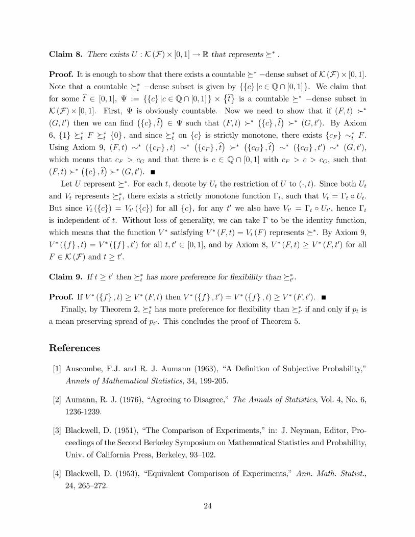
Claim 8. There exists U : K (F)� [0; 1]! R that represents �� :
Proof. It is enough to show that there exists a countable �� �dense subset of K (F)� [0; 1].Note that a countable ��t �dense subset is given by ffcg jc 2 Q \ [0; 1]g. We claim that
for some bt 2 [0; 1], := ffcg jc 2 Q \ [0; 1]g ��bt is a countable �� �dense subset in
K (F)� [0; 1]. First, is obviously countable. Now we need to show that if (F; t) ��
(G; t0) then we can �nd�fcg ;bt� 2 such that (F; t) ��
�fcg ;bt� �� (G; t0). By Axiom
6, f1g ��t F ��t f0g ; and since ��t on fcg is strictly monotone, there exists fcFg ��t F .Using Axiom 9, (F; t) �� (fcFg ; t) ��
�fcFg ;bt� �� �fcGg ;bt� �� (fcGg ; t0) �� (G; t0),
which means that cF > cG and that there is c 2 Q \ [0; 1] with cF > c > cG, such that
(F; t) ���fcg ;bt� �� (G; t0).
Let U represent ��. For each t, denote by Ut the restriction of U to (�; t). Since both Utand Vt represents ��t , there exists a strictly monotone function �t, such that Vt = �t � Ut.But since Vt (fcg) = Vt0 (fcg) for all fcg, for any t0 we also have Vt0 = �t � Ut0, hence �tis independent of t. Without loss of generality, we can take � to be the identity function,
which means that the function V � satisfying V � (F; t) = Vt (F ) represents ��. By Axiom 9,
V � (ffg ; t) = V � (ffg ; t0) for all t; t0 2 [0; 1], and by Axiom 8, V � (F; t) � V � (F; t0) for all
F 2 K (F) and t � t0.
Claim 9. If t � t0 then ��t has more preference for �exibility than ��t0.
Proof. If V � (ffg ; t) � V � (F; t) then V � (ffg ; t0) = V � (ffg ; t) � V � (F; t0).Finally, by Theorem 2, ��t has more preference for �exibility than ��t0 if and only if pt is
a mean preserving spread of pt0. This concludes the proof of Theorem 5.
References
[1] Anscombe, F.J. and R. J. Aumann (1963), �A De�nition of Subjective Probability,�
Annals of Mathematical Statistics, 34, 199-205.
[2] Aumann, R. J. (1976), �Agreeing to Disagree,�The Annals of Statistics, Vol. 4, No. 6,
1236-1239.
[3] Blackwell, D. (1951), �The Comparison of Experiments,�in: J. Neyman, Editor, Pro-
ceedings of the Second Berkeley Symposium on Mathematical Statistics and Probability,
Univ. of California Press, Berkeley, 93�102.
[4] Blackwell, D. (1953), �Equivalent Comparison of Experiments,�Ann. Math. Statist.,
24, 265�272.
24
[5] Dekel, E., B. Lipman, and A. Rustichini (2001), �Representing Preferences with a
Unique Subjective State Space,�Econometrica, 69, 891�934.
[6] Dekel, E., B. Lipman, A. Rustichini, and T. Sarver (2007), �Representing Preferences
with a Unique Subjective State Space: Corrigendum,�Econometrica, 75, 591�600. (See
also supplemental appendix.)
[7] De Olivera, H. (2012) �Axiomatic Foundations for Rational Inattention.�mimeo
[8] Dillenberger, D., and P. Sadowski (2012a), �Generalized Partition and Subjective Fil-
tration,�mimeo.
[9] Dillenberger, D., and P. Sadowski (2012b), �Subjective Learning,�PIERWorking Paper
number 12-007.
[10] Ergin, H., and T. Sarver (2010), �A Unique Costly Contemplation Representation,�
Econometrica, 78, 1285-1339.
[11] Gollier, C., (2001), �The Economics of Risk and Time,�The MIT Press, 0-262-07215-7.
[12] Harsanyi, John. C., (1967), �Games with Incomplete Information Played by "Bayesian"
Players, I-III,�Management Science, Vol. 14, No. 3, 159-182.
[13] Higashi, Y., K. Hyogo, and N. Takeoka (2009), �Subjective Random Discounting and
Intertemporal Choice,�Journal of Economic Theory, 144 (3), 1015�1053.
[14] Hyogo, K. (2007), �A Subjective Model of Experimentation,� Journal of Economic
Theory, 133, 316�330.
[15] Kihlstrom, R. E., (1984), �A Bayesian Exposition of Blackwell�s Theorem on the Com-
parison of Experiments,�in Bayesian Models of Economic Theory (M. Boyer and R. E.
Kihlstrom, Eds.), pp. 13-32, Elsevier, Amsterdam.
[16] Kreps, D. (1979), �A Representation Theorem for �Preference for Flexibility,�Econo-
metrica, 47, 565�577.
[17] Krishna, R. V., and P. Sadowski (2012), �Dynamic Preference for Flexibility,�mimeo.
[18] Lleras, J.S. (2011), �Expected Knowledge,�unpublished manuscript.
[19] Mihmn M., and M.K. Ozbek, (2012) �Decision Making with Rational Inattention,�
mimeo.
25

[20] Takeoka, N. (2005), �Subjective Prior over Subjective States, Stochastic Choice, and
Updating,�unpublished manuscript.
[21] Takeoka, N. (2007), �Subjective Probability over a Subjective Decision Tree.�Journal
of Economic Theory, 136, 536�571.
26


