Doru-Stefan Irimescu

ABSOLUTE POSITION

MEASUREMENT AND CONTROL FOR

WÄRTSILÄ ENGINE DURING

SLOW TURNING

Technology and Communication

2018

VAASAN AMMATTIKORKEAKOULU

UNIVERSITY OF APPLIED SCIENCES

Information Technology

ABSTRACT

Author Doru-Stefan Irimescu

Title Absolute position measurement and control for

Wärtsilä engine during slow turning

Year 2018

Language English

Pages 77

Name of Supervisor Jukka Matila

Fredrik Backman

The thesis work was carried out for Wärtsilä Finland Oy’s Engine Performance

and Control department of the Marine Solutions division. The paper studied the

implementation of the absolute position measurement and control of Wärtsilä’s

engine crank angle during the slow turning procedure. The topic came out as an

endeavor to improve the functionality of Wärtsilä’s engine control system, as at

the moment of its proposal the crank angle had remained unknown during the en-

tire slow turning sequence. The aim of the thesis was to implement a solution that

would facilitate the precise adjustment of the engine position after the slow turn-

ing had proceeded.

Slow turning is a marine engine procedure during which the engine is being ro-

tated at low speeds, in order to check the presence of water in the cylinders, as this

can lead to hydrostatic locking, and thus cause severe damages during normal,

high-speed operation. Given the fact that the tachometers used by the Wärtsilä en-

gine systems at the outset of this study were of inductive nature, it was not possi-

ble to monitor rotational velocities below 100 rotations per minute. This meant

that not only the engine stopped at an unknown position after slow turning, but

also that, in the case that maintenance needed to be effectuated, manual engine po-

sitioning was required.

Research was conducted with the aim of investigating the current system, and

finding its limitations. In addition, the necessary work for implementing, testing

and documenting an improved alternative was performed.

Keywords Wärtsilä, Engine control, Automation, Slow turning

CONTENTS

TIIVISTELMÄ

ABSTRACT

1 INTRODUCTION ....................................................................................... 10

1.1 Wärtsilä OY ........................................... Error! Bookmark not defined.

1.2 Wärtsilä UNIC ..................................................................................... 13

1.3 Objective and topic of choice ............................................................... 15

1.4 Implementation plan ............................................................................. 15

2 THEORY AND BACKGROUND INFORMATION ................................... 17

2.1 Electromechanical control system components ..................................... 17

2.1.1 The four-stroke cycle of the marine diesel engine...................... 18

2.1.2 Hydrostatic lock and slow turning ............................................. 19

2.1.3 Engine speed and phase measurement ....................................... 19

2.1.4 Absolute engine position ........................................................... 22

2.1.5 Hall-effect and inductive sensors............................................... 24

2.1.6 Engine control unit module ....................................................... 24

2.1.7 Frequency converter and motor ................................................. 25

2.2 Software ............................................................................................... 26

2.2.1 Model-based design .................................................................. 26

2.2.2 Matlab and Simulink ................................................................. 27

2.2.3 Finite state machine .................................................................. 28

2.2.4 Stateflow .................................................................................. 29

2.2.5 Wärtsilä applications ................................................................. 31

2.2.6 Wärtsilä Simulink Development Environment .......................... 32

3 CURRENT SYSTEM INVESTIGATION ................................................... 34

3.1 Slow turning application ....................................................................... 34

3.1.1 Main application structure ......................................................... 34

3.1.2 Inputs ........................................................................................ 35

3.1.3 Control ..................................................................................... 36

3.1.4 Outputs ..................................................................................... 38

3.2 Slow turning control logic .................................................................... 39

3.2.1 Task control .............................................................................. 39

3.2.2 Sequence control ....................................................................... 41

4 SOLUTION IMPLEMENTATION ............................................................. 42

4.1 Absolute position measurement simulation ........................................... 42

4.1.1 Sensor signal simulation ........................................................... 45

4.1.2 Direction measurement simulation ............................................ 49

4.1.3 Position measurement simulation .............................................. 51

4.2 Absolute position measurement implementation ................................... 56

4.3 Manual engine position control implementation ................................... 56

4.3.1 Application section ................................................................... 58

4.3.2 Process section .......................................................................... 62

4.4 Code generation and compilation ......................................................... 65

5 TESTING ENVIRONMENT AND RESULTS ............................................ 66

5.1 Simulation ............................................................................................ 66

5.2 Laboratory test ..................................................................................... 68

6 CONCLUSION AND FURTHER IMPROVEMENTS ................................ 72

5

LIST OF ABBREVIATIONS

BDC Bottom dead center

CAN Controller area network

CCM Cylinder Control Module

COM Communications Module

ECU Engine control unit

EPC Engine performance and control

ESM Engine Safety Module

FMT First missing tooth

FSM Finite state machine

HIL Hardware in loop

Hydrolock Hydrostatic lock

IOM Input/Output Module

LED Light emitting diode

LOP Local Operator Panel

RGB Red green blue

RPM Revolutions per minute

TDC Top dead center

UNIC Unified control

WASP Wärtsilä application software package

WMAP Wärtsilä modular application platform

6

WSDE Wärtsilä Simulink Development Environment

LIST OF FIGURES AND TABLES

Figure 1. Engine Performance and Control organization 2017 p. 12

Figure 2. UNIC system layout p. 13

Figure 3. UNIC modules. From left to right: LOP, COM, CCM, IOM, ESM p. 14

Figure 4. Thesis implementation and engineering design plan p. 15

Figure 5. The measurement and control target setup. p. 17

Figure 6. Four stroke cycle of a diesel engine p. 18

Figure 7. Camshaft and crankshaft connection p. 20

Figure 8. Engine speed sensors p. 20

Figure 9. Engine Flywheel hole location and pulse train generation p. 21

Figure 10. Phase/stroke detection p. 22

Figure 11. Flywheel and camshaft angular position p. 22

Figure 12. Inductive speed measurement p. 23

Figure 13. Hall-effect principle p. 24

Figure 14. Hall-effect speed measurement p. 24

Figure 15. Vacon frequency converter p. 25

Figure 16. Model-based design lifecycle p. 26

Figure 17. Simulink block. p. 28

Figure 18. On/Off temperature controller p. 28

Figure 19. Stateflow superstate and its substates p. 30

7

Figure 20. Superstate with two substates active concurrently p. 30

Figure 21. An example of different state actions’ usage p. 31

Figure 22. WSDE structure p. 32

Figure 23. Slow turning control application structure p. 34

Figure 24. Inputs subsystem p. 35

Figure 25. Control subsystem p. 37

Figure 26. Rotation pulses block p. 37

Figure 27. Outputs subsystem p. 38

Figure 28. The Control state machine p. 39

Figure 29. The task control super state p. 40

Figure 30. The sequence control super state p. 41

Figure 31. Rotate engine superstate p. 42

Figure 32. Speed and Phase signal simulation p. 44

Figure 33. Speed sensor 1 and speed sensor 2 signal simulation p. 44

Figure 34. Engine position and phase generator p. 45

Figure 35. Speed and phase initialization p. 46

Figure 36. First speed signal generator subsystem p. 46

Figure 37. Pulse counter from 0 to number of teeth-1 and back p. 46

Figure 38. Second speed signal generator subsystem p. 47

Figure 39. Phase generator subsystem p. 47

Figure 40. Phase pulse counter p. 48

8

Figure 41. Phase signal logic subsystem p. 48

Figure 42. Set direction subsystem p. 49

Figure 43. Rising edge detection subsystem p. 49

Figure 44. Falling edge detection subsystem p. 49

Figure 45. Direction measurement p. 50

Figure 46. Direction calculation p. 50

Figure 47. Speed sensors and direction timing diagram p. 50

Figure 48. Angle measurement p. 51

Figure 49. Position measurement p. 51

Figure 50. Angle measurement subsystem p. 52

Figure 51. First missing tooth logic p. 53

Figure 52. First missing tooth detection p. 53

Figure 53. Enabled subsystem block of the missing tooth detection subsystem p. 53

Figure 54. State machine responsible with the angle logic calculations p. 54

Figure 55. Speed increment and decrement functions p. 54

Figure 56. Engine position, phase, rotation direction and angle measurement p. 55

Figure 57. Input ISO codes p. 56

Figure 58. Output ISO codes p. 56

Figure 59. Position measurement implementation p. 57

Figure 60. User input ISO codes p. 58

Figure 61. Tolerance calculation p. 59

9

Figure 62. Engine position set interrupt variable logic p. 59

Figure 63. “SetSequenceType” superstate p. 60

Figure 64. Control logic implementation inside “ManualSequences” p. 61

Figure 65. Set position or rotate to position p. 61

Figure 66. Rotate to position subsystem p. 62

Figure 67. Function used for selecting the direction of rotation p. 62

Figure 68. User input simulation p. 63

Figure 69. Set desired engine position subsystem p. 63

Figure 70. Writing the process ISO codes to the application p. 64

Figure 71. Hall-effect sensor simulation p. 64

Figure 72. First test result, setpoint 12 degrees p. 66

Figure 73. Second test result, setpoint 360 degrees p. 66

Figure 74. Third test result, 0 degrees setpoint p. 67

Figure 75. Lab test setup p. 68

Figure 76. Speed signals and direction of rotation for the entire procedure p. 69

Figure 77. Speed signals and direction of rotation zoomed p. 69

Figure 78. Angular position during the first test p. 70

Figure 79. Flywheel angular position step decrement p. 70

Figure 80. Speed signals and direction of rotation p. 71

Figure 81. Angular position change during the whole second test p. 71

10

1 INTRODUCTION

As automation is rapidly evolving and becoming more ubiquitous in every industrial applica-

tion, the marine industry has to adapt to the ever more demanding requirements of modern

engine control technologies, and incorporate advanced automated features into the design, op-

eration and manufacturing process.

As a leading name in the marine industry, Wärtsilä has been keeping the pace with the

development of automation technologies, introducing the Wärtsilä Unified Controls

(UNIC) engine control system, allowing extensive monitoring and control of their en-

gines’ performance and functionality.

1.1 Wärtsilä Oy

“Wärtsilä is a global leader in advanced technologies and complete lifecycle solutions for

the marine and energy markets. By emphasising sustainable innovation and total effi-

ciency, Wärtsilä maximises the environmental and economic performance of the vessels

and power plants of its customers.” /1/

Wärtsilä is targeting three business sectors, namely: Marine Solutions, Energy Solutions,

and Services. The main company mission is to improve current technologies involved in

the marine and energy markets, with a strong focus on customer needs, environment, en-

ergy efficiency and performance. /2/

The Marine Solutions department is the leading provider of innovative products and in-

tegrated solutions in the marine, oil and gas industries, offering the most complete palette

of services on Earth, covering all the marine market segments, such as: Oil and Gas, Mer-

chant, Cruise and Ferry, Navy and Special Vessels. /2/

The Marine Solutions’ products offer /3/:

Environmental Excellence, through efficient fuel consumption and reduced emis-

sions

Fuel Flexibility, by introducing dual-fuel engine technologies and alternative

fuel compatibility, such as ethane or bio fuels

11

Operational Efficiency, by integrating a vessel’s propulsion, control and automa-

tion systems into the most efficient combination, capable of achieving impressing

results, such as the world’s most efficient 4-stroke diesel engine

Lifecycle Support, by offering non-stop coverage of all the locations on Earth

Integrated Solutions, by “integrating all the various elements that go into produc-

ing the most efficient and cost-effective operational performance”

The Energy Solutions department is a “leading global energy system integrator offering

a broad range of environmentally sound solutions”, with a wide range of offers, including:

”ultra-flexible internal combustion engine based power plants, utility-scale solar PV

power plants, energy storage & integration solutions, as well as LNG terminals and dis-

tribution systems” /1/

The Energy Solutions’ products offer /4/:

Energy efficiency, by adopting power plants composed of multiple generation

units, capable of efficiently serving on part load even in the most demanding con-

ditions, and by introducing the proprietary Flexicycle™ solution, that combines

the advantages of simple cycle plants with the efficiency of combined cycle plants

Fuel Flexibility, by designing multi-fuel plants that are able to run on gaseous

fuels as well as renewables

Operational flexibility, by enabling the power plants to be configured for suiting

different needs

Dependability, as the power plants are 99% available and reliable, the plants be-

ing ready to supply power whenever it is needed

Development and financial services, by offering support, assistance and advice

to their clients

Project Services, by planning, leading, managing and executing projects for cus-

tomers

Lifecycle support, by offering parts and maintenance services

The Services department is supporting the customers throughout the whole product

lifecycle, the company’s service network consisting of approximately 11,000 profession-

als in 160 global locations, delivering services to more than 12,000 customers every year.

/1/

12

The Services business offers /5/:

Lifecycle solutions, by signing service agreements that ensure reliable perfor-

mance ranging from fuel receival to energy supply

Services and parts, by displaying a wide range of services and solutions

1.1.1 The Engine Performance and Control department

The main role of the EPC department is to develop the engine process performance and

functionality, with a mission of converting customers’ requirements and needs into opti-

mized performance solutions and providing engine process and controls expertise, in or-

der to achieve the most competitive level of quality, performance and cost through the

entire lifecycle of the product. The department’s vision is to connect engine processes

and controls, with the aim of maximizing performance. /6/

As it can be noted from Figure 1, the EPC department is split into different teams, each

with a specific area of expertise. The main attribution of the Engine Controls and Systems

team is to develop and implement the architecture of the engine control system and soft-

ware.

Therefore, it comes naturally that the thesis is written for the Engine Controls and Sys-

tems, as most of the tasks related to embedded systems development and implementation

are performed in there.

Figure 1. Engine Performance and Control organization 2017

13

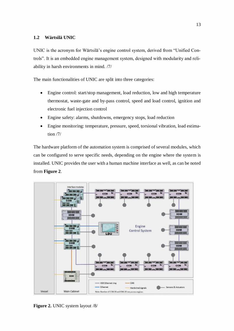
1.2 Wärtsilä UNIC

UNIC is the acronym for Wärtsilä’s engine control system, derived from “Unified Con-

trols”. It is an embedded engine management system, designed with modularity and reli-

ability in harsh environments in mind. /7/

The main functionalities of UNIC are split into three categories:

Engine control: start/stop management, load reduction, low and high temperature

thermostat, waste-gate and by-pass control, speed and load control, ignition and

electronic fuel injection control

Engine safety: alarms, shutdowns, emergency stops, load reduction

Engine monitoring: temperature, pressure, speed, torsional vibration, load estima-

tion /7/

The hardware platform of the automation system is comprised of several modules, which

can be configured to serve specific needs, depending on the engine where the system is

installed. UNIC provides the user with a human machine interface as well, as can be noted

from Figure 2.

Figure 2. UNIC system layout /8/

14

The main components of the UNIC system are the following modules /8/:

LOP, the local operator panel: a display unit, consisting of RGB LED illuminated

buttons and a touch screen, as well as an emergency button, offering an interface

to the automation system, and providing the operator with useful engine infor-

mation. Its key functions are local/remote control selection, local starting and

stopping, trip and shutdown reset, emergency stop, local emergency speed setting

and status information about engine running modes, possible faults and log of

events

COM, the communications module: the main gateway between the vessel systems

and the UNIC system, supporting multiple field busses and interface such as Mod-

bus, OPC, hardwired I/O, CAN, etc. Besides communications, its attributions con-

sist of several control functions, as well as offering an interface for software and

configuration update and management. Typically two such modules are used on

the engine, for redundancy reasons

CCM, the cylinder control module: the main responsibility is to control the com-

bustion process, monitoring all the injection and combustion functions, and the

inlet valve timing of the cylinder firing. Depending on the number of cylinders

available on the engine, the number of CCM modules can vary

IOM, the input/output module: these modules carry out all the engine-specific

measurements, and thus are placed in proximity to the sensors or sensing devices.

Their number can vary depending on more factors, such as engine type, applica-

tion or the number of cylinders used

ESM, the Engine Safety Module: performing all the safety checks related to pos-

sible engine failures, these modules deliver fault-specific actions, such as engine

shutdown in case of over speeding.

Figure 3. UNIC modules. From left to right: LOP, COM, CCM, IOM ,ESM /8/

15

1.3 Objective and topic of choice

The objective of this document is the analysis of the current implementation and improve-

ment of the engine control unit applications regarding slow turning and speed monitoring.

As a measurable target for the objective’s completion, the positioning of the engine at a

preset angular position after slow turning has occurred is chosen, along with an investi-

gation of the current system. As supporting objectives, the direction of rotation is de-

tected, and the fastest route towards the desired angular position is being followed.

The current topic is preferred as a subject of study, as it incorporates elements of embed-

ded systems software analysis and design, automata theory, model-based design using

Matlab’s Simulink and Stateflow, electrical automation, measurements and control, en-

compassing all the major issues studied during the last four years in the Information Tech-

nology degree at Vaasa University of Applied Sciences.

1.4 Implementation plan

The thesis work (the engineering design), as well as its structure (the actual paper) follow

the cycle presented in Figure 4:

Figure 4. Thesis implementation and engineering design plan

16

The thesis starts with a given problem to be solved, described in the abstract and intro-

duction chapters. It continues with the study of the concepts needed to fully understand

the topic in question, as well as the gathering of relevant information that clarifies the

technical, specific details of the issues to be solved, process covered in the theory and

background information chapter. The analysis of the current situation follows, where the

system to be improved is being researched, in the current system investigation chapter.

The proposed solutions and their application are documented in the solution implemen-

tation chapter. The testing environment and methodology are presented in the testing en-

vironment and results chapter. The results obtained after testing the solution are presented

in the testing environment and results chapter, as well. Finally, a discussion leading to

conclusions and further possible improvements is proposed in the conclusion and further

improvements chapter.

Only one complete engineering design cycle described above is documented in this work.

17

2 THEORY AND BACKGROUND INFORMATION

In this chapter, the theory necessary to achieve the required setup (Figure 5) for reaching

the objective of the thesis is presented. Furthermore, this chapter is split into two distinct

parts: the first part deals with the components of the electromechanical system, while the

second part introduces the software tools and methodologies used for performing this

work.

Figure 5. The measurement and control target setup.

2.1 Electromechanical control system components

In order to understand the background of the thesis, some preliminary information must

be conveyed regarding the electronic and mechanical parts of the control system. This

part includes a detailed explanation of the process, the sensors, and the controller. The

electromechanical control system (Figure set) consists of the UNIC engine control unit,

acting as the controller, the Frequency converter and the motor, acting as the actuator, the

Flywheel and the Camshaft as the process, and the speed and phase sensors as the meas-

urement that closes the feedback loop.

18

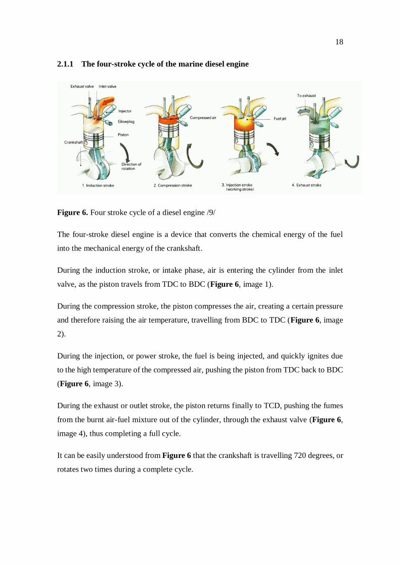
2.1.1 The four-stroke cycle of the marine diesel engine

Figure 6. Four stroke cycle of a diesel engine /9/

The four-stroke diesel engine is a device that converts the chemical energy of the fuel

into the mechanical energy of the crankshaft.

During the induction stroke, or intake phase, air is entering the cylinder from the inlet

valve, as the piston travels from TDC to BDC (Figure 6, image 1).

During the compression stroke, the piston compresses the air, creating a certain pressure

and therefore raising the air temperature, travelling from BDC to TDC (Figure 6, image

2).

During the injection, or power stroke, the fuel is being injected, and quickly ignites due

to the high temperature of the compressed air, pushing the piston from TDC back to BDC

(Figure 6, image 3).

During the exhaust or outlet stroke, the piston returns finally to TCD, pushing the fumes

from the burnt air-fuel mixture out of the cylinder, through the exhaust valve (Figure 6,

image 4), thus completing a full cycle.

It can be easily understood from Figure 6 that the crankshaft is travelling 720 degrees, or

rotates two times during a complete cycle.

19

2.1.2 Hydrostatic lock and slow turning

The piston has to be able to travel freely inside the cylinder, with as few resistance as

possible (Figure 6).

In the faulty case in which the cylinder is filled with an incompressible fluid that takes

up at least as much volume as the volume of the cylinder at TDC, hydro lock occurs,

thus creating the necessary conditions for a failure to take place, if the engine is being

operated in this state. /10/

Slow turning is a preventive method that aims to detect the defective condition ex-

plained in the above paragraph, by rotating the engine at a low speed and monitoring the

cylinder pressure and actuator current consumption, while the pistons are actuated sev-

eral times between TDC and BDC by the rotating crankshaft.

2.1.3 Engine speed and phase measurement

The engine speed is one of the most important process variables, being used for speed

and fuel demand control or injection timing calculation, if the engine is equipped with

electronic fuel injection.

As can be noted from Figure 7, the four-stroke cycle of the engine (one complete rotation

of the camshaft) takes place during two full rotations of the crankshaft and the flywheel.

This happens due to the fact that the camshaft is connected to the crankshaft via the timing

belt, with a typical sprocket gear ratio of 2 to 1, the crankshaft rotating in the same time

with the flywheel. However, it is not mandatory for the connection to be realized with a

timing belt, as similar connections can be achieved with systems of geared wheels.

Thus, it is not possible to use the speed measurement alone for calculating the absolute

engine position. Consequently, it is imperative that additional sensors are required for

measuring the engine phase using a half moon disc, placed at the end of the camshaft.

/11/

20

Figure 7. Camshaft and crankshaft connection /12/

For each tooth of the flywheel there is a pair of holes, except for a missing one, corre-

sponding to the TDC engine position. There are two speed sensors, namely a primary and

a secondary one, for redundancy reasons, mounted close to the flywheel lateral side, as

shown in Figure 8.

Figure 8. Engine speed sensors /11/

21

The sensor (Figure 8) outputs a pulse for every hole passing in front of it, and so the

speed can be easily calculated if the distance and timing between two holes are known.

For detecting the precise angular position of the engine, one hole pair is missing, gener-

ating a gap in the incoming pulse train. The missing hole pair is located in such way that

the next pulse is exactly at the top dead center of the A1 cylinder. Even though the speed

sensors use separate hole tiers, due to the fact that they are stacked perpendicular to the

direction of motion, the phase difference between the incoming signals is 0. On Wärtsilä

engines, the number of holes is 120 – 1 (Figure 9).

Figure 9. Engine Flywheel hole location and pulse train generation /11/

One of the big limitations of this current configuration is that the rotation direction cannot

be measured with the aid of the sensor configuration described above, and if the absolute

positioning of the flywheel is required, this is immediately becoming an issue: when the

electric motor rotating the flywheel is disengaged, this produces some back and forth

oscillations of the wheel, and so the position cannot be correctly calculated anymore.

Once the rotational speed measurement is settled, the working phase/stroke of the cylin-

der A1 needs to be monitored as well, with the aid of phase detection sensors, as otherwise

it is unclear which stroke corresponds to the TDC signal. Again, two sensors are being

used for redundancy reasons.

The principles behind the phase detection measurement can be easily understood from

Figure 10: Attached to the camshaft’s end, there is a disk which is having one protruding

22

half. This configuration allows the phase sensor to output a positive pulse at 180° before

the TDC of the cylinder A1, and remain high until 180° after TDC.

Figure 10. Phase/stroke detection

2.1.4 Absolute engine position

In contrast to the relative engine position, that would be represented in respect to the

starting/current flywheel position, the absolute position considers the entire four-stroke

cycle as two rotations of the flywheel (Figure 11), therefore 720 degrees, establishing a

bijective mapping between the flywheel and camshaft position and the calculated angle.

Figure 11. Flywheel and camshaft angular position

2.1.5 Hall-effect and inductive sensors

There are two types of sensors widely used in the engine RPM measurements, namely

inductive and Hall-effect sensors.

The inductive sensors (Figure 12) have a coil placed in front of a magnetic field, and

once a metal object passes in front of the magnetic field, it changes the magnetic flux

23

density inside and around the coil, thus inducing a voltage at the ends of the coil. Due to

the Faraday’s law of induction (equation 1), the induced electromotive force depends pro-

portionally on the rate of change in magnetic flux density in respect to time, and thus

imposes a lower limit on the working speed /13/. For Wärtsilä engines, the lower speed

limit at which the sensors are guaranteed to work is 100 RPM, making it impossible to

monitor slow turning speed pulses in the range of 1 to 6 RPM.

𝜀 = −𝑁𝑑𝜙𝐵

𝑑𝑡 (1)

Figure 12. Inductive speed measurement /13/

Hall-effect sensors (Figure 14) present a great advantage over inductive sensors in the

way that they do not depend on the rate of change of the magnetic flux density. Instead,

these sensors depend on the magnetic force acting on electric charges moving inside a

conductor placed in a magnetic field, force that generates a potential difference across the

lateral sides of the conductor, which can be further amplified by means of semiconductor

technology (Figure 13). Therefore, in contrast to the inductive sensors that depend upon

the rate of change of the incident magnetic field, the hall-effect sensors depend on the

magnetic field alone (equation 2)

𝑉ℎ =𝐼𝐵

𝑛𝑒𝑑 (2)

24

Figure 13. Hall-effect principle /14/

Hence, these sensors can be used for measuring slower speeds and phase changes. The

output of the signal produced by the sensor is constant in amplitude, regardless of the

speed of rotation, as only the frequency of the signal is proportional with the frequency

of rotation. /13/

Figure 14. Hall-effect speed measurement

2.1.6 Engine control unit module

The only required UNIC module for the slow turning application to work is COM-10, as

it features the necessary PC communication capabilities, as well as sensor reading and

actuator communication capabilities.

25

The relevant specifications of COM-10 are listed below:

One Ethernet RJ45 port, used for PC communication with the engine control unit

configuration software, capable of reaching speeds of up to 100Mbit/s

Four CAN galvanically isolated ports, used for frequency converter communica-

tion, capable of reaching speeds of up to 1Mbit/s

Four Analog/Digital input channels, used for reading the speed and phase sensors’

data, capable of handling from 0 to 32 volts in the digital input mode

Sampling rate of up to 100Hz for applications and sensor inputs

2.1.7 Frequency converter and motor

Figure 15. Vacon frequency converter

A frequency converter (Figure 15) is a device that changes the frequency of its input

power, in order to command a frequency-driven actuator. For this project’s purpose, the

actuator is an AC synchronous motor that is coupled via a geared wheel to the engine

flywheel, and its rotational speed is controlled by the frequency converter.

The frequency converter provides an interface to the control application via the CAN

communication protocol, offering information about the speed of rotation and current

draw of the synchronous motor, as well as giving the user the possibility to change the

RPM of the motor by using simple commands.

26

It is important to note here that the ensemble comprising of the synchronous motor and

the toothed wheel is usually referenced to as the “turning gear” throughout the control

application. The coupling and decoupling of the turning gear to the flywheel is accom-

plished with a solenoid-based system.

Hence, by connecting the frequency converter to the UNIC COM-10 module, the appli-

cation development engineer can manipulate the turning gear by making use of specific

Simulink blocks.

2.2 Software

The UNIC ECU acts as the digital controller for the purposes of this thesis, therefore all

the logic and algorithms required for the absolute position control are being programmed

by making use of state of the art software tools. In this section, the software environment

deployed for the completion of this document is presented, together with some funda-

mental theoretical concepts demanded for understanding the need for introducing the fol-

lowing tools.

2.2.1 Model-based design

Model-based design is a paradigm that aids representing and solving problems related to

complex systems. The system model is at the center of the development process, through-

out the design lifecycle (Figure 16) /15/

Figure 16. Model-based design lifecycle

27

The main difference between the model-based and traditional design approach is that,

while the second one involves complex structures and making use of software code, the

first approach allows the designers to define, develop and improve plant models by using

specific building blocks. /16/

Consequently, this new method of developing systems brings several benefits to the en-

gineering teams, such as: the model can be tested, refined and improved at any time dur-

ing the developmental process, errors are more easily found, as testing and validations

are constantly performed, embedded code can be automatically generated from the system

model, which makes it a powerful tool that saves time and optimizes the design flow. /17/

2.2.2 Matlab and Simulink

Matlab is an acronym for “matrix laboratory”, used for naming a proprietary program-

ming language and numerical computing environment, created by the American corpora-

tion MathWorks. /18/

Used by millions of engineers and scientists worldwide, Matlab facilitates the analysis

and design of systems from diverse areas of technology, such as automotive, marine, spa-

tial, medical, electrical and cellular networks to name a few. Some key features of this

environment are: a high-level language intended for scientific and engineering computa-

tions, graphical tools for data visualization, add-on toolboxes for diverse engineering and

scientific applications. /19/

The numerous add-ons make Matlab a very popular software development environment

and a first choice for many engineering companies that focus of research and develop-

ment. One of the most powerful add-ons that Matlab offers is Simulink, an environment

that facilitates model-based design of dynamic systems, particularly in the fields of auto-

matic control and signal processing. /20/

By providing the convenient and efficient code generation feature, together with the ro-

bust and highly-abstracted model structure, Simulink enables Wärtsilä to develop up to

20% faster code, and have a productivity increase of up to 300%. /21/

When a new system model is being conceived with Simulink, typically a block diagram

is firstly created, that encompasses the time dependencies between the system’s inputs

28

and outputs, as well as its interior states, with the connecting lines representing the sys-

tem’s signals. A block (Figure 17) can be, for example, a mathematical or logic function,

or can consist of more inner blocks, in which case it would be called a subsystem. /20/

Figure 17. Simulink block

2.2.3 Finite state machine

Finite state machines are used for describing systems that can have one out of a finite

number of states at any time. This model of computation is useful when describing event-

driven systems, namely systems that react by changing their state based on their inputs.

Many devices nowadays can be thought of as being state machines, such as traffic lights,

combination locks, elevators, etc. /22/

A basic example of a FSM is presented in Figure 18. The initial (default) state is ON, and

if the temperature exceeds 23 degrees, it transitions to the OFF state. Consequently, if the

temperature falls below 23 degrees, it switches back into the ON state.

Figure 18. On/Off temperature controller

When modelling state machines, the next state, X(n+1) can be described by a mathemat-

ical function of the current state, X(n), and the machine’s inputs, u. /23/

𝑋(𝑛 + 1) = 𝑓(𝑋(𝑛), 𝑢) (3)

29

Based on equation (3), two different types of state machines can be distinguished: the

ones where the next state depends on both inputs and the current state, called Mealy ma-

chines, and the ones where the next state depends solely on the current state, called Moore

machines.

2.2.4 Stateflow

Stateflow is a control logic add-on for the Matlab/Simulink environment, created for

modelling and simulating combinatorial and sequential decision logic for hybrid systems,

where the continuous dynamics are represented by Simulink. Made with model logic,

fault management and task scheduling in mind, Stateflow aids the design engineer with

state machine animations as well as numerous tools for testing and debugging the appli-

cation in early stages, before implementation. Stateflow integrates seamlessly with Sim-

ulink, enabling automatic code generation for the modeled state machines. /24/

The main component of the Stateflow environment is the chart, a custom block that de-

fines a state machine and encloses one or multiple states. There are three types of charts

available: /25/

Classic, the default machine type. It is a combination of Mealy and Moore state

machines. This chart shall be used only when the other two types can be re-

garded as an infeasible option, as it has several limitations, in terms of error

messages, code generation efficiency and algebraic loop handling

Mealy, where the output is a function of inputs and state. It presents several ad-

vantages over the classic chart type, although it cannot be used to model feed-

back loops

Moore, where the output is a function of state only. It offers the most efficient

code generation implementation, as well as the possibility to add feedback loops

if needed

The main component of the chart is the state, a block that describes an operating mode

of the FSM. A state that encloses multiple other child states (substates) is referred to as

a superstate (Figure 19).

30

Figure 19. Stateflow superstate and its substates /26/

The substates of a superstate can execute exclusively, in which case the decomposition

of the superstate is OR, or in parallel, in which case the decomposition of the superstate

is called AND. The borders of the block indicate its decomposition type: solid borders

mean exclusive, while dashed borders (Figure 20) mean parallel execution.

Figure 20. Superstate with two substates active concurrently /27/

Besides the part that indicates the name of the state, the label of a state includes, option-

ally, five state actions: /28/

Entry action, which is executed only once when the state becomes active

During action, which is executed as long as the state remains active

Exit action, which is executed only once, right before the state becomes inactive

On action, which specifies an event that can occur while the state is active, and a

handler for that event

Bind action, which allows only the binding state and its children to broadcast the

bound event

Figure 21 illustrates a typical example of state action declaration usage

31

Figure 21. An example of different state actions’ usage /28/

2.2.5 Wärtsilä applications

The architecture upon which the engine control software is built is called WMAP, the

Wärtsilä Modular Application Platform. This structure defines three abstraction and re-

sponsibility layers, namely:

Application layer, that contains a set of software modules that implement the nec-

essary logic for specific engine control functionalities

Platform software layer, that contains lower level software implementations of

communication protocols, data and signal processing, configuration storage, and

various features required by the application layer

Hardware abstraction layer, that provides easy access to hardware features for the

platform software layer

The application software development is exclusively within the Wärtsilä area of respon-

sibility, as it is implementing the highest level of abstraction between the engine control

unit hardware and engine functionality. All of the software described in this document is

incorporated in this layer.

32

2.2.6 Wärtsilä Simulink Development Environment

The Wärtsilä Simulink Development Environment (WSDE) is a Matlab/Simulink envi-

ronment created to aid the application (engine control software module) engineer with

developing and simulating an engine-specific application control logic.

Figure 22. WSDE structure /29/

The main structure of the WSDE can be seen in Figure 22: the main Simulink file consists

of the application itself and the simulated process. The process simulation takes as inputs

the application’s outputs, and its outputs are fed into the application’s inputs.

The WSDE supports:

Process simulation

Automatic code generation

Unit testing

HIL testing:

o Process in the loop

o Control in the loop

33

The Wärtsilä Simulink Development Environment comes with an extensive set of rules

and guidelines that recommend good modelling practices, originating from the Math-

works Automotive Advisory Board set of guidelines.

The WSDE guide document is structured into two main parts, the first part concerning all

the guidelines necessary for standardized application development, such as: naming con-

ventions, model appearance, model architecture, Simulink and Stateflow implementation

practices, while the second part is assisting the engineer with using the WSDE, offering

detailed information about how to create and test control models using Simulink and

Stateflow.

It is mandatory for the new application development engineer to familiarize with the

WSDE guidelines, as they convey the necessary discipline, routines and formats for cre-

ating an easily understandable and readable piece of software that can be later tested,

improved and deployed by other engineers without any prior background of the current

implementation.

34

3 CURRENT SYSTEM INVESTIGATION

This chapter proposes an investigation of the current implementation of the UNIC system

automation layers responsible with the slow turning sequence, as it has been performed

by the Wärtsilä engineers up until the point of this document’s creation. Considering that

certain confidentiality formalities have to be followed, some figures are blurred.

3.1 Slow turning application

The slow turning application in its current state is primarily used for detecting fluid pres-

ence in the cylinders. In this section, the Simulink architecture of the application is dis-

cussed.

3.1.1 Main application structure

The main structure of the slow turning application follows the recommended WSDE

model architecture (WSDE 1.1.4), and it is thus split into three layers (Figure 23):

Inputs, placed on the left side of the model, furtherly divided into specific blocks

Control, placed in the middle of the model, furtherly divided into specific sub

systems

Outputs, placed on the right side of the model, furtherly divided into specific

blocks

Figure 23. Slow turning control application structure

35

3.1.2 Inputs

The Inputs block unfolds into a subsystem (Figure 24) that acquires the relevant data for

the Control block and routes it its “in” port (Figure 23)

Figure 24. Inputs subsystem

The data is split into:

Constants subsystem, which contains immutable values used in control calcula-

tions

Configuration parameters subsystem, which contains configurable values read

from the engine configuration, such as revolution counter type (phase, engine or

camshaft revolutions, camshaft teeth), system type (pneumatic or electric), slow

turning type, etc

ISO codes subsystem, which reads data container values from the engine control

unit, depending on the configuration parameters selected. Some examples of those

values are: turning gear current consumption, turning gear status, remote standby

request, etc

36

Accessors subsystem, which reads periodically the system time counter in milli-

seconds

Machinery protection subsystem, which communicates with the engine safety and

checks, for example, if shutdown is currently active

3.1.3 Control

The Control block unfolds into a subsystem (Figure 25) that contains a Stateflow chart,

comprising of the main slow turning state machine, a bus selector block that routes all the

necessary inputs from the “in” port of the Control block to the chart, and a bus creator

block that routes all the necessary outputs from the chart to the “out” port of the Control

block (Figure 30, middle)

37

Figure 25. Control subsystem

At this level, the rotation pulses are calculated inside the RevCounter block and fed into

the state machine as inputs (Figure 26)

Figure 26. Rotation pulses block

38

Currently, the number of engine revolutions is counted based on the camshaft speed sen-

sors, as they are the only hall-effect sensors capable of monitoring speeds as low as the

slow turning process requires.

3.1.4 Outputs

The Outputs block contains a subsystem (Figure 27) that writes the control data to the

engine control system that in turn interprets it and actuates the plant.

The data is split into the following subsystems:

ISO codes, that update the UNIC system with the current information about the

slow turning type, status and progress

Triggers, that update the UNIC system with the necessary information, such as

slow turning failure, pre-warning, active, etc signals only when the new data is

made available, in order to decrease the computational load on the system

Runtimes, that update the UNIC system with current information with the runtime

variables, such as slow turning status or sequence type

LogMessages, that update in a triggered manner the UNIC system with logs re-

garding the status of the slow turning sequence that can be used to debug or mon-

itor the application

Figure 27. Outputs subsystem

39

3.2 Slow turning control logic

In this section, the Stateflow architecture of the slow turning application is discussed.

The control state machine superstate (Figure 28) is split into two parts: the “TaskControl”

checks and sets a sequence to run, and once a valid sequence has been selected (“Se-

quenceType” != “SEQ_NONE” ), “SequenceControl” runs the actual sequence. This state

also calculates the total progress of the slow turning sequence

Figure 28. The Control state machine

3.2.1 Task control

The task control (Figure 29) consists of an initial state, the “SlowturningDisabled” state,

which is entered by default. “SlowturningEnabled” superstate can be entered only if the

slow turning activation is not set to “disabled”.

40

Figure 29. The task control super state

“CheckSlowturningPerformed”, “SetSequenceType” and “CheckTGLubePerformed”

states are executing in parallel, and can exit anytime if either slow turning is disabled or

the engine blow is set to true.

“SetSequenceType” monitors the active engine mode, and sets the sequence type accord-

ing to the selected inputs. Once the sequence is selected, the “TaskControl” superstate

transitions to the “SequenceControl” superstate.

“CheckSlowturningPerformed” verifies the current status of slow turning (which can be

failed, aborted or performed), and decides if slow turning is required again, for example

if enough time has passed after it has been performed.

“CheckTGLubePerformed” checks when is the turning gear lubrication required again,

and sets the status of “TG lube”. Turning gear lubrication is a special part of the slow

turning sequence, where the turning gear motor is being rotated in order to lubricate a

sealed bearing, which otherwise would wear out due to the engine vibrations pushing the

lubricant on the sides of the bearing.

41

3.2.2 Sequence control

The function of this superstate (Figure 30) is to perform the requested slow turning se-

quence, while monitoring any abort signals that might interrupt the process. At the start

of the sequence, logs are being created to inform the type of the procedure that is going

to be run. When the sequence is about to stop, before exiting the SequenceControl state,

logs regarding the outcome of the procedure are being generated (aborted, failed, per-

formed, failed handshake with frequency converter, etc)

Figure 30. The sequence control super state

This thesis studies the electric part of the sequence control, as it is more practical to con-

trol the absolute position of the flywheel using a toothed gear attached to it and spun by

an electric motor. As a result, the rest of the sequence control sub chapter analyses the

electric slow turning procedure.

In order to initialize the electric slow turning, a handshake with the frequency converter

needs to take place. If the handshake is successful, two actions can be performed: spin

the turning gear motor, for lubrication purposes, or engage the turning gear and continue

with the slow turning sequence.

42

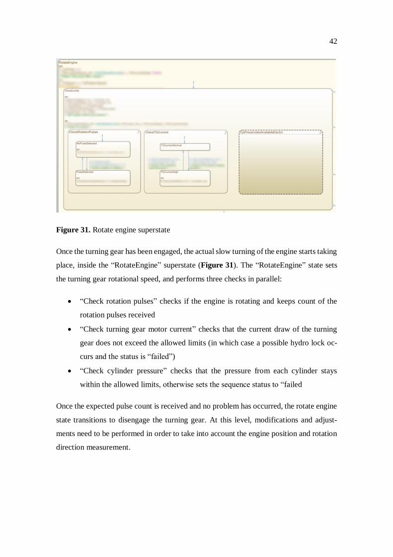
Figure 31. Rotate engine superstate

Once the turning gear has been engaged, the actual slow turning of the engine starts taking

place, inside the “RotateEngine” superstate (Figure 31). The “RotateEngine” state sets

the turning gear rotational speed, and performs three checks in parallel:

“Check rotation pulses” checks if the engine is rotating and keeps count of the

rotation pulses received

“Check turning gear motor current” checks that the current draw of the turning

gear does not exceed the allowed limits (in which case a possible hydro lock oc-

curs and the status is “failed”)

“Check cylinder pressure” checks that the pressure from each cylinder stays

within the allowed limits, otherwise sets the sequence status to “failed

Once the expected pulse count is received and no problem has occurred, the rotate engine

state transitions to disengage the turning gear. At this level, modifications and adjust-

ments need to be performed in order to take into account the engine position and rotation

direction measurement.

43

4 SOLUTION IMPLEMENTATION

The application-level solution implementation consists of four main parts: the absolute

position measurement simulator, the absolute position measurement implementation, the

control logic and process simulation for manually setting the desired position, and the

code generation and compilation.

As of the date of this work’s inception, the only way of monitoring the engine revolutions

during slow turning is through an intermediary application that outputs the number of

camshaft revolutions, as hall-effect sensor support had not been yet implemented in the

system for flywheel low-speed monitoring. Therefore, a position measurement prototype,

which reads speed and phase signals from dedicated flywheel and camshaft sensors is

presented in this part of the document, together with the control logic necessary for ma-

nipulating the engine revolutions during slow turning by making use of the absolute po-

sition.

4.1 Absolute position measurement simulation

Because the system in question is fairly complex, the signal generation and measurement

are firstly simulated, as the latter cannot be tested and designed without having the former.

Once a working prototype is achieved, the measurement, together with the control logic

are implemented into the actual application, and the signal generator is used for the pro-

cess simulation part.

The flywheel has 120 teeth, out of which one is missing. The first tooth after the missing

one represents 360 (or 720) degrees, as two flywheel rotations complete one four stroke

cycle.

If both falling edge and rising edge detection is used, the measurement error is plus minus

3 degrees at the missing tooth and 1.5 degrees between any two teeth. The number of

flywheel teeth, however, can vary, between the test setup, which uses 30-1 teeth, and the

lab engine, which uses 120-1 teeth, hence the simulator has to be configurable for the

number of flywheel teeth. Therefore, the measurement error for the laboratory wheel is

plus minus 12 degrees at the missing tooth, and 6 degrees between any two teeth.

44

In order to know in which half of the four stroke cycle the engine position is located,

another signal is critical: the phase signal, coming from the camshaft phase sensor. The

phase signal changes, ideally, in the middle of the distance between two missing teeth –

thus, on the 60th tooth-. A simulation of the speed and phase signals can be seen in Figure

32.

Figure 32. Speed and Phase signal simulation

In addition to the speed and position measurement, the direction of rotation has to be

calculated. This is possible to achieve, as one hall-effect module consists of two speed

sensors placed next to each other with a small offset between them, such that the current

pulse is being detected firstly by the sensor number one, and then by the sensor number

two. A simulation of the two speed signals is presented in Figure 33.

45

Figure 33. Speed sensor 1 and speed sensor 2 signal simulation

4.1.1 Sensor signal simulation

Before implementing the control logic on the application side, a simulator for the speed

and phase signals is made for the process part, that takes into account the variable number

of flywheel teeth. The signals generated by the simulator are shown in Figure 32 and

Figure 33.

Figure 34. Engine position and phase generator

The clock of the Engine position and phase generator (Figure 34), called the “Flywheel

clock” is a signal generator block with amplitude 1, and frequency configured in another

Simulink file (Figure 35). The period of this clock represents the time elapsed between

two consecutive flywheel teeth. For debugging purposes, the signal generator’s output

can be enabled or disabled from the “Enable signal” block. The “Speed1 generator” block

generates the speed signal with a missing tooth on the 119th position for a flywheel with

120 teeth, and the “Speed2 generator” simply adds a delay to the first speed signal, mim-

icking the phase difference between the two hall-effect sensors. The “phase generator”

block uses the same clock to derive the necessary phase signal. The “setDir” block swaps

between the “Speed1 generator” and “Speed2 generator” signals, in order to simulate a

change in direction.

46

Figure 35. Speed and phase initialization

The “Speed1 generator” block (Figure 36) unfolds into a subsystem that counts up and

down, depending on direction, pulses from 0 to nteeth-1, outputs the flywheel clock signal

normally, and bypasses it on the nteeth-1th pulse. The pulse counter’s block content is

presented in Figure 37.

Figure 36. First speed signal generator subsystem

47

Figure 37. Pulse counter from 0 to number of teeth-1 and back

The “Speed2 generator” block (Figure 38) simply adds a delay measured in seconds on

the “Speed1” signal, specified in another Simulink file. However, this delay cannot be

negative, consequently the “Speed2” signal is always lagging the “Speed1” signal. The

difference between the two speed signals is depicted in Figure 33.

Figure 38. Second speed signal generator subsystem

The last part of the absolute position simulator is the phase signal. If the speed pulse trains

correspond to signals coming from the two sensors located on the flywheel, the phase

signal simulates the output of the sensor located on the camshaft. The phase generation

comprises two subsystems (Figure 39), the first one being responsible with generating a

pulse counter, from 0 to 239 for a flywheel of 120 teeth, and the second one being re-

sponsible with generating a high or low output, depending on the pulse counter value.

Figure 39. Phase generator subsystem

The phase pulse counter counts either up or down, depending on direction, from zero to

two times the number of flywheel teeth minus one, and then starts again from zero. (Fig-

ure 40)

48

Figure 40. Phase pulse counter

If the phase pulse counter’s output lies between one half and three halves of the total

number of teeth, the phase signal is high. If the contrary happens (the pulse counter's

output lies below one half, or between three halves and two times the total number of

teeth), it is low (Figure 41). Therefore, during 120 pulses (one full flywheel rotation) the

phase signal is high, and during another 120 pulses, the phase signal is low, for a flywheel

which has 120-1 teeth.

Figure 41. Phase signal logic subsystem

The last component of the sensor signal simulation is the direction of rotation. This be-

havior can be modelled by swapping the speed signals between each other, as in Figure

42.

49

Figure 42. Set direction subsystem

4.1.2 Direction measurement simulation

Before measuring the absolute angular position, the direction of rotation has to be known.

This measurement happens on both the rising and falling edge of the first speed signal.

As the rising and falling edge detection blocks from Simulink do not work for WSDE

code generation, special subsystems are created with this purpose in mind (Figure 43 and

Figure 44)

Figure 43. Rising edge detection subsystem

Figure 44. Falling edge detection subsystem

50

Figure 45. Direction measurement

In Figure 45, the direction measurement subsystem is presented. The inputs are the speed

sensor one and two, and the outputs represent the direction, as well as the rising and fall-

ing edge detection signals, which are needed by the angle measurement. The direction

calculation subsystem (Figure 46) outputs either a one or a zero (Figure 47).

Figure 46. Direction calculation

Figure 47. Speed sensors and direction timing diagram

51

4.1.3 Position measurement simulation

The position measurement block is presented in Figure 48. The inputs are the direction,

rising and falling edge detection signals of the first speed sensor, system time, and phase.

The outputs are the angle and first missing tooth detection. Because the application data

can be communicated only as 32-bit signed integers, the angle has to be expressed in

decidegrees, thus 1.5 degrees are represented and communicated as 15 decidegrees.

Figure 48. Angle measurement

The output of the position measurement can be seen in Figure 49, as it ranges from 0 to

7200 for a flywheel made of 120 teeth.

Figure 49. Position measurement

The “fmt” output is a signal that specifies the first occurrence of the missing tooth. This

is a crucial piece of information for the system implementation, as in real life the engine

does not always spin at constant speeds. If a sudden deceleration of the flywheel occurs,

a larger-than-usual gap would appear between two consecutive teeth, and it could be mis-

52

taken for a missing tooth. Therefore, for accurately pinpointing the engine angle, the fly-

wheel position will have to be “synchronized” with the measurement system, by being

rotated at a constant speed until a missing tooth appears. After this point, if all the speed

pulses are monitored, the engine position can be known under any circumstances.

The angle measurement subsystem is shown in Figure 50. The upper part of the system

computes the first missing tooth, while the lower part contains the signal processing logic

for determining the precise engine angle.

Figure 50. Angle measurement subsystem

In addition to the common Simulink blocks, this subsystem also encloses two Stateflow

charts, used to abstract the sequential logic that leads to the desired results. The “Angle

logic” state machine needs information about the missing tooth occurrence, thus the “First

missing tooth detection” has to be executed first. The “FMT logic” (Figure 51) state ma-

chine constantly checks for an occurrence, and once this happens, it switches its output

and remains high, for synchronization (a one-time event). During further development,

specific conditions could be defined for resetting the first missing tooth, in case the syn-

chronization is lost.

53

Figure 51. First missing tooth logic

The first missing tooth detection (Figure 52) is based on the principle of a constant delay

between any two consecutive tooth pulses, and a larger gap when the missing tooth oc-

curs, longer than one and a half times the value of the previous delay.

Figure 52. First missing tooth detection

The enabled subsystem (Figure 53) is being activated every time the speed signal goes

high, reads the current system time, subtracts it from the previous reading, and outputs a

time result. The result is then compared to the missing tooth time duration (Figure 52),

which is considered to be at least 1.5 times its preceding tooth duration. The final result

is either a zero or a one, the latter corresponding to a positive occurrence.

Figure 53. Enabled subsystem block of the missing tooth detection subsystem

54

The angle logic state machine (Figure 54) starts in the default “noCount” state. Once the

first missing tooth happens, meaning that synchronization has occurred, the state changes,

based on the direction of rotation. Depending on the phase signal, the angle starts from 0

or 360 degrees, if the direction is 1, or from 0 or 354 degrees, if the direction is -1 and the

flywheel has 120 teeth. After this, the state remains in the “positiveDirection” or “nega-

tiveDirection” until the direction of rotation changes. The change variable is used to mon-

itor the change in direction. The absolute position is recalculated periodically in these two

states, with the help of the “speedInc” and “speedDec” functions (Figure 55)

Figure 54. State machine responsible with the angle logic calculations

Figure 55. Speed increment and decrement functions

55

Figure 56. Engine position, phase, rotation direction and angle measurement

In Figure 56 the complete simulation is shown, and the signal path can be clearly traced

between its component systems. This is a crucial part of the solution implementation pro-

cess, as it displays all the necessary building blocks in one single file. Until this point, a

working backbone has been achieved.

The next steps of the implementation involve placing the necessary blocks into the pro-

cess side, namely the speed1, speed2, phase and direction generators, and placing the

measurement blocks, namely the rotation direction and angle measurement into the ap-

plication side of the slow turning control slx file, according to the WSDE guideline.

56

4.2 Absolute position measurement implementation

As the measurements described in the above subchapter requires speed and phase signal

information, the following input ISO codes are created and read within the slow turning

application (Figure 57)

Figure 57. Input ISO codes

In addition to the codes above, three new ISO codes are created and written to the engine

control unit, making it possible to monitor the direction, angle and missing tooth synchro-

nization status (Figure 58)

Figure 58. Output ISO codes

57

Once the inputs and outputs are correctly defined and implemented, the calculation blocks

are inserted inside the application’s control subsystem (Figure 59)

Figure 59. Position measurement implementation

4.3 Manual engine position control implementation

The manual position control implementation subchapter describes the control logic and

the building blocks that allow for the most important feature of this project to exist, sub-

sequently setting a target crank angle, and moving the flywheel to that position. It is im-

portant to state that designing the user interface which is used for communicating the

implicit values is not a part of the thesis, as the functionalities described are being tested

by making use of the engine control unit monitoring and configuration software tool,

provided by Wärtsilä.

Following the WSDE guideline, this subchapter is furtherly split into two sections, re-

spectively the Application section, that deals with implementing the actual control logic

that runs on the engine control unit, and the Process section, which simulates the actuated

plant’s response to the control effort, that helps testing and debugging the project at an

early phase, without the need of deployment on a real engine.

58

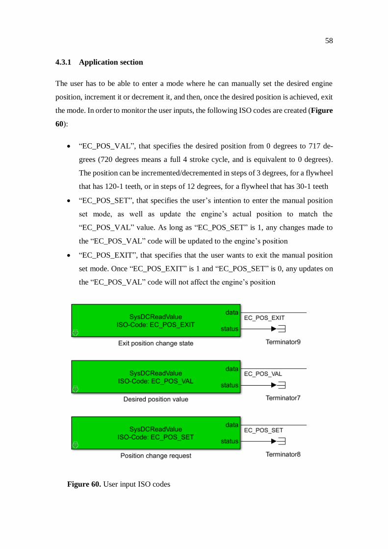
4.3.1 Application section

The user has to be able to enter a mode where he can manually set the desired engine

position, increment it or decrement it, and then, once the desired position is achieved, exit

the mode. In order to monitor the user inputs, the following ISO codes are created (Figure

60):

“EC_POS_VAL”, that specifies the desired position from 0 degrees to 717 de-

grees (720 degrees means a full 4 stroke cycle, and is equivalent to 0 degrees).

The position can be incremented/decremented in steps of 3 degrees, for a flywheel

that has 120-1 teeth, or in steps of 12 degrees, for a flywheel that has 30-1 teeth

“EC_POS_SET”, that specifies the user’s intention to enter the manual position

set mode, as well as update the engine’s actual position to match the

“EC_POS_VAL” value. As long as “EC_POS_SET” is 1, any changes made to

the “EC_POS_VAL” code will be updated to the engine’s position

“EC_POS_EXIT”, that specifies that the user wants to exit the manual position

set mode. Once “EC_POS_EXIT” is 1 and “EC_POS_SET” is 0, any updates on

the “EC_POS_VAL” code will not affect the engine’s position

Figure 60. User input ISO codes

59

These user inputs can be later on accessed via a human-machine interface, such as a local

display unit.

Before implementing the control logic for manual position control, a tolerance for the

desired position misplacement has to be established (Figure 61). This represents the max-

imum number of tolerable error, when positioning the flywheel. The addition of this pa-

rameter helps reducing the oscillations resulting from the high moment of inertia of the

flywheel.

Figure 61. Tolerance calculation

The control logic for manually setting the position is added in the “ManualSequences”

state, which is a substate of the “SetSequenceType” superstate. Once the user has set the

EC_POS_SET to 1 and EC_POS_EXIT to 0, the “ManualSequences” state can be en-

tered. In order to facilitate this, a function called “ManualPositionRequest” has been cre-

ated (see Figure 62). This function sets a variable called EC_POS_SET_INT either true

or false.

Figure 62. Engine position set interrupt variable logic

60

If EC_POS_SET_INT is true, the active substate of the “SetSequenceType” superstate

will change from “CheckEngineMode” to “ManualSequences” (Figure 63)

Moreover, if “EC_POS_SET_INT” is true, and the substate “StandbyModeSequences”

of the “SetSequenceType” superstate is active, the state will be changed immediately to

“CheckEngineMode”.

Figure 63. “SetSequenceType” superstate

Inside the “ManualSequences” state (Figure 64), if “EC_POS_SET_INT” is true, the

turning gear is engaged, the engine is being rotated to the desired position, and once the

desired position has been achieved, the “SetPosition” state remains active until the user

either changes the desired position again, or exits the procedure by setting

“EC_POS_EXIT” to be true. It is to be noted that the “EC_POS_EXIT” signal has a

higher priority than the “EC_POS_SET_INT” signal, as the former triggers the exiting of

the “SetPosition” procedure regardless of the latter’s value. As the desired position is

specified in degrees, a conversion to decidegrees is being made inside the calculations.

61

Figure 64. Control logic implementation inside “ManualSequences”

The “SetRot” function (Figure 65) decides the transition between the “RotateToPosition”

and “SetPosition” states, based on the desired and actual engine position.

62

Figure 65. Set position or rotate to position

At this point, the “RotateToPosition” block (Figure 66) rotates the engine and checks the

fastest available route (Figure 67) for reaching the set point.

Figure 66. Rotate to position subsystem

Figure 67. Function used for selecting the direction of rotation

4.3.2 Process section

On the process side, a simulation of the user inputs is made, and the simulated values are

written to the ISO codes that the application reads and interprets as user commands. In

Figure 68, the Simulink blocks that implement the functionalities described above can be

observed.

63

The “Set desired eng pos” subsystem simply takes care of the user inputs, either the “POS

SET INC” or “POS SET DEC”, and keeps track of the desired position value by incre-

menting or decrementing it in steps of 3 degrees. The initial desired position starts at 0.

The subsystem’s contents can be seen in Figure 69.

Figure 68. User input simulation

Figure 69. Set desired engine position subsystem

The signals shown above are routed to a bus that links them to the outputs block, where

they are written to the relevant ISO codes, as in Figure 70. On the application side, these

codes are written and processed as it is explained in this document.

64

Figure 70. Writing the process ISO codes to the application

The Hall-effect simulation block (Figure 71) comprises of the blocks described in the

absolute position measurement simulation subchapter. The “speed” signal, in this case,

represents the turning gear’s speed of rotation. The block is enabled if the speed is non-

zero, and the direction is set by the sign of the speed signal. The “spd1”, “spd2” and

“phase” outputs are routed to the output ISO codes, as they represent the simulated sensor

signals.

Figure 71. Hall-effect sensor simulation

65

4.4 Code generation and compilation

Once a working application and process model have been achieved, the next solution

implementation step involves using the feature that makes Simulink such a powerful en-

gineering tool, namely the automatic code generation.

The compilation of the application software requires a special environment called

“Devbox” to be installed, which is Lubuntu-based virtual machine, that contains all the

necessary programs for generating the binaries required by the hardware modules in order

to run the newly-created applications.

The next step is choosing a baseline for the engine configuration, onto which the appli-

cation can be added. This whole practice happens in accordance with the WASP guide-

line, which defines the Wärtsilä Application Software Package directory structure, and

sets the rules on how the procedure is to be handled. This step is being achieved with the

help of Wärtsilä systems engineers. The slow turning application files are then updated

with the newly-generated ones.

Next, using UniTool, the Wärtsilä software for engine configuration and monitoring, the

additional files that are needed are generated, such as schemas and headers. These files

are particularly relevant for the integration of the application into the UniTool software,

for engine configuration and tuning purposes.

Finally, the compilation process can begin, and once it is ready, the binary-containing

archives that are loaded on the hardware modules are generated. The next step involves

choosing an appropriate engine package, with the guidance of Wärtsilä system engineers.

An engine package is a collection of software application modules that are configured for

running on a particular engine. It contains, among other features:

configurations for the application parameters

configurations for the ECU hardware modules

communication protocol configurations

machinery safeties, that are configurable model-based algorithms for implement-

ing various safety behaviors

Once a suitable engine package has been selected, the generated binaries are being loaded.

66

5 TESTING ENVIRONMENT AND RESULTS

The testing is performed in two stages, namely the simulation and the laboratory testing.

However, the laboratory test does not involve a real engine, but a 30-1 teeth miniature

flywheel, for obvious reasons, such as accessibility and ease of deployment.

5.1 Simulation

The first test involves starting from an unsynchronized position, with the setpoint of 12

degrees. As seen in Figure 72, the simulation stops rotating at 180 decidegrees, or 18

degrees, because of the 6 degrees tolerance.

Figure 72. First test result, setpoint 12 degrees

Figure 73. Second test result, setpoint 360 degrees

67

The second test involves starting from the previous position (18 degrees), and reaching a

setpoint of 360 degrees. As seen in Figure 73, the simulation stops rotating at 348 de-

grees, because of the 12 degrees tolerance at the missing tooth position.

The third test involves starting from the previous position (348 degrees), and reaching a

setpoint of 0 degrees. As seen in Figure 74, the simulation stops rotating at 6 degrees,

because of the 6 degrees tolerance.

Figure 74. Third test result, 0 degrees setpoint

In conclusion, the simulation tests are successfully passed, with all the results according

to the expectations, and within the tolerance limits.

68

5.2 Laboratory test

Figure 75. Lab test setup

In the Wärtsilä laboratory (Figure 75), the test setup involves a custom-made flywheel,

with two missing teeth, a half-moon disk and 58 teeth in total. One full rotation of this

laboratory wheel simulates two rotations of a 30-1 teeth flywheel, together with the cam-

shaft phase signal. Hence, it is a sufficient device for testing the software implementation.

The wheel is connected directly to the electric motor which is actuated by a frequency

converter, thus the turning gear is missing.

Because of the larger diameter of the new hall-effect speed sensor module, it is not pos-

sible to mount it perpendicular to the flywheel’s teeth, as the designated space on the

metal frame that holds the flywheel is too narrow. Therefore, a compromise is made, in

order to locate the sensor as closely as possible to its functional position.

69

The following test is performed and analyzed in this subchapter: the flywheel starts from

a random, unknown position, and the target destination is 24 degrees (or 240 decidegrees).

The speed signals incoming from the speed 1 and 2 sensors, together with the direction

of rotation are shown in Figure 76. The magnitude of the direction signal signifies clock-

wise rotation, for a value of one, and counter-clockwise rotation, for a value of zero. The

signals are being read by the ECU at a frequency of 100 Hertz. In Figure 76 it can be

noted that, once the flywheel gets past a point, it changes direction during the last pulse.

In practice, this can always happen.

Figure 76. Speed signals and direction of rotation for the entire procedure

Figure 77. Speed signals and direction of rotation zoomed

In Figure 77, the incoming speed signals are magnified, together with the direction signal.

70

In Figure 78, the flywheel’s angular position change from the beginning to end of the test

is being traced. Moreover, it can be noted that, after synchronization, the angular position

is starting from 0 degrees.

Figure 78. Angular position during the first test

In Figure 79, the last change in angular position is presented. It can be noted that, even

if the motor stopped rotating the flywheel at 30 degrees, because of the 6 degrees of tol-

erance, the flywheel rotated by itself 6 degrees counter clockwise, to 24 degrees. If the

contrary had happened, so that the flywheel had rotated clockwise to 36 degrees, the con-

trol application would have brought it to 30 degrees.

Figure 79. Flywheel angular position step decrement

71

The next test is to move from 24 degrees to 648 degrees. The results are shown in the

figures below, in Figure 80 and Figure 81.

Figure 80. Speed signals and direction of rotation

Figure 81. Angular position change during the whole second test

From Figure 81, it can be noted that the rotation stops at 642 degrees, for a setpoint of

648 degrees. This, again, is perfectly consistent with the 6 degrees tolerance for the 30-1

teeth flywheel.

72

6 CONCLUSION AND FURTHER IMPROVEMENTS

The objective of this paper was to investigate and improve the current slow turning Wärt-

silä engine control application, by making it possible to monitor the absolute angular po-

sition of the engine flywheel during the entire 4-stroke cycle, as well as its direction of

rotation. Furthermore, a means of manipulating the flywheel position during maintenance

was desired.

In addition, this work strove to bring considerable improvements to the actual Wärtsilä

engine control software, as well as help introducing, integrating and documenting the new

improved hall-effect sensors and their benefits.

In this thesis, a working simulation of the actual process described above, as well as the

process control logic are designed and documented. As the results described in the chapter

testing environment and results are showing, the required objectives are met, with a rea-

sonable accuracy.

Although a functional application is achieved, there are further improvements that can be

made:

Firstly, the application’s update period is 10 milliseconds, meaning that the appli-

cation cannot run more often than 100 times in one second. This constraint im-

poses serious limitations on the speed of rotation of the flywheel, because of the

small gap between the two speed sensors. Consequently, either the application

update rate should be increased, or a means of first missing tooth desynchroniza-

tion detection could be implemented, so that the application would attempt to re-

synchronize in that case

Secondly, a new metal frame for the laboratory flywheel should be designed, with

the measurements according to the new hall-effect sensor module specifications,

as it has been really hard to manually position the sensor accurately for receiving

valid signals

Thirdly, due to the high moment of inertia of the flywheel, if the turning speed is

increased beyond a particular point, the system will start oscillating about the de-

sired position, without being able to stop the flywheel in time. If such “high”

73

speeds of positioning are desired, a more complex algorithm that takes into ac-

count the rate of change of the positioning error, as well as the actual error, with

the purpose of adjusting the rotation speed accordingly could be devised, such as

a PD controller

Lastly, a full test should be performed on the real engine

On a personal note I can affirm that, during the making of this thesis I have acquired new,

relevant and interesting knowledge regarding my field of studies that has broadened my

perspectives on the industry of automation engineering.

Finally, I would like to thank all the teachers from the Vaasa University of Applied Sci-

ences for their help, in particular to Dr. Seppo Mäkinen and Mr. Jukka Matila, for their

sustained support and academic expertise. Moreover, I would like to express my sincere

gratitude to the Wärtsilä EPC’s “Engine Controls and Systems” department, in particular

to Hedvik Sören and Fredrik Backman, for offering me this unique opportunity of pro-

fessional development.

REFERENCES

/1/ This is Wärtsilä. Accessed 22.03.2018

https://www.wartsila.com/about

/2/ Wärtsilä corporation. Accessed 22.03.2018

https://cdn.wartsila.com/docs/default-source/investors/financial-materials/corpo-

rate-presentations/corporate-presentation-2017.pdf?sfvrsn=2

/3/ Wärtsilä solutions for Marine and Oil & Gas Markets. Accessed 22.03.2018

https://cdn.wartsila.com/docs/default-source/marine-documents/segment/bro-

chure-marine-solutions-2017.pdf?sfvrsn=28

/4/ Wärtsilä-What we do. Accessed 22.03.2018

https://www.wartsila.com/energy/what-we-do

/5/ Wärtsilä-Services. Accessed 22.03.2018

https://www.wartsila.com/services

/6/ Product performance documentation. Accessed from Wärtsilä intranet

22.03.2018

/7/ Wärtsilä UNIC engine control system for gas and dual fuel engines. Accessed

22.03.2018

https://www.wartsila.com/services/areas-of-expertise/services-catalogue/electri-

cal-automation-services/wartsila-unic-engine-control-system-for-gas-and-dual-

fuel-engines

/8/ Wärtsilä UNIC Engine Control System Overview. Accessed 23.03.2018

https://cdn.wartsila.com/docs/default-source/product-files/engines/brochure-o-e-

unic-ms.pdf

/9/ 2-Stroke vs. 4-Stroke Engines. Accessed 23.03.2018

https://dieselengineregistry.wordpress.com/2-stroke-vs-4-stroke-engines/

/10/ Hydrolock Wikipedia page. Accessed 23.03.2018

https://en.wikipedia.org/wiki/Hydrolock

/11/ UNIC System Description. Accessed from Wärtsilä intranet 23.03.2018

/12/ Overhead camshaft. Accessed 23.03.2018

https://www.howacarworks.com/illustrations/engine-with-overhead-camshaft

/13/ Inductive and hall effect rpm sensors explained. Accessed 23.03.2018

https://www.linkedin.com/pulse/inductive-hall-effect-rpm-sensors-explained-kiril-

mucevski/

/14/ The Hall Effect. Accessed 23.03.2018

http://hyperphysics.phy-astr.gsu.edu/hbase/magnetic/Hall.html

/15/ Model-based design Matlab. Accessed 23.03.2018

https://se.mathworks.com/help/simulink/gs/model-based-de-

sign.html?s_tid=gn_loc_drop

/16/ Model-based design Wikipedia page. Accessed 23.03.2018

https://en.wikipedia.org/wiki/Model-based_design

/17/ How small engineering teams adopt model-based design. Accessed 23.03.2018

https://www.mathworks.com/content/dam/mathworks/mathworks-dot-com/cam-

paigns/portals/files/adopting-model-based-design/how-small-engineering-teams-

adopt-model-based-design.pdf

/18/ Matlab Wikipedia page. Accessed 23.03.2018

https://en.wikipedia.org/wiki/MATLAB

/19/ Matlab getting started guide. Accessed 23.03.2018

https://se.mathworks.com/help/pdf_doc/matlab/getstart.pdf

/20/ Simulink getting started guide. Accessed 23.03.2018

https://se.mathworks.com/help/pdf_doc/simulink/sl_gs.pdf

/21/ Wärtsilä Accelerates Engine Control Development Using Production Code

Generation

https://se.mathworks.com/company/user_stories/wrtsil-accelerates-engine-control-

development-using-production-code-generation.html

/22/ Finite state machine Wikipedia page. Accessed 23.03.2018

https://en.wikipedia.org/wiki/Finite-state_machine

/23/ Overview of Mealy and Moore Machines. Accessed 23.03.2018

https://se.mathworks.com/help/stateflow/ug/overview-of-mealy-and-moore-ma-

chines.html

/24/ Stateflow documentation. Accessed 23.03.2018

https://se.mathworks.com/help/stateflow/index.html

/25/ Overview of Mealy and Moore Machines. Accessed 23.03.2018

https://se.mathworks.com/help/stateflow/ug/overview-of-mealy-and-moore-ma-

chines.html

/26/ Stateflow state hierarchy. Accessed 23.03.2018

https://se.mathworks.com/help/stateflow/ug/state-hierarchy.html

/27/ Stateflow state decomposition. Accessed 23.03.2018

https://se.mathworks.com/help/stateflow/ug/state-decomposition.html

/28/ Stateflow states. Accessed 23.03.2018

https://se.mathworks.com/help/stateflow/ug/states.html

/29/ WSDE guideline. Accessed from Wärtsilä intranet 23.03.2018