Ac breakdown in near-atmospheric pressure noble gases: II. Simulations

This article has been downloaded from IOPscience. Please scroll down to see the full text article.

2011 J. Phys. D: Appl. Phys. 44 224003

(http://iopscience.iop.org/0022-3727/44/22/224003)

Download details:

IP Address: 131.155.108.56

The article was downloaded on 13/05/2011 at 08:49

Please note that terms and conditions apply.

View the table of contents for this issue, or go to the journal homepage for more

Home Search Collections Journals About Contact us My IOPscience

IOP PUBLISHING JOURNAL OF PHYSICS D: APPLIED PHYSICS

J. Phys. D: Appl. Phys. 44 (2011) 224003 (13pp) doi:10.1088/0022-3727/44/22/224003

Ac breakdown in near-atmosphericpressure noble gases: II. SimulationsA Sobota1, J van Dijk1 and M Haverlag1,2

1 Eindhoven University of Technology, Department of Applied Physics, Postbus 513,5600MB Eindhoven, The Netherlands2 Philips Lighting, LightLabs, Mathildelaan 1, 5600JM Eindhoven, The Netherlands

E-mail: a.sobota@tue.nl

Received 30 November 2010, in final form 27 January 2011Published 12 May 2011Online at stacks.iop.org/JPhysD/44/224003

AbstractThe effect of frequency on the characteristics of ac-driven breakdown processes in 0.7 barargon is investigated by means of a two-dimensional fluid model. The geometry represents thehigh intensity discharge lamp burner with a pin–pin electrode system forming a 7 mmelectrode gap. The breakdown process is considered in the frequency range between 60 kHzand 1 MHz. The appearance of the discharge and the influence of the voltage frequency on itscharacteristics obtained in the simulations is in good agreement with the experimental data(accompanying paper—Sobota et al 2011 J. Phys. D: Appl. Phys. 44 224002, special issue onLS12/WLED3 symposium). The role of the secondary electron emission from the electrodesurfaces is demonstrated and linked to the lowering of the threshold voltage with the increasein frequency observed both in experiment and model.

(Some figures in this article are in colour only in the electronic version)

1. Introduction

Breakdown processes driven by high-frequency ac voltagehave been a topic investigated only for specific applications, forexample for controlling and suppressing the surface dischargeson printed circuit boards and similar semiconductor-basedsystems [1]. Related to this, the problem of surface andvolume partial discharges occurring in partial vacuum hasbeen of interest in aerospace insulating technology [2]. Onthe other hand, ac discharges found their use in the scienceof material processing, where the glow discharges createdin atmospheric pressure possess the uniformity that is notpresent in filamentary discharges obtained in pulsed mode [3–5]. Also, some research on ac-driven discharges has been donefor the lighting industry when trying to design ignition conceptsfor high-frequency operated lamps [6] or lower their ignitionvoltage [7].

When talking about the breakdown processes driven byhigh-frequency voltage, it is necessary to distinguish betweenthe frequency ranges, as the discharge forms in different waysat different frequencies. The important parameter is actuallya specific combination of the frequency, the electrode gap andthe pressure of the gas, but if we imagine a system where

the electrode gap and the gas pressure are kept constant,we can analyse the effect of the voltage frequency on thebreakdown process. At low frequencies, provided that thevoltage amplitude surpasses the threshold for breakdown, abreakdown event takes place in every half of every voltagecycle and it can be thought of as pulsed breakdown with veryslow-rising voltage.

Increasing the frequency and keeping the voltage leveljust above the threshold for breakdown brings us to the rangewhere breakdown events take more than one voltage cycle tocomplete. Even though the time necessary for the developmentof the charged channel to cross the gap can vary from just afraction of a voltage cycle to few tens of voltage cycles [8],the whole breakdown process still takes several cycles tocomplete, as the charge build-up at the electrode tips thatprecedes the formation of the ionized channel is necessary forits subsequent growth. The electron losses in this frequencyrange are drift-dominated. In a configuration with two-pinelectrodes the charged particle production volume is locatedaround the electrode tips, as this is the area of highest electricfield in the system. This production volume is also close to theelectrode surface, bringing forward the potential significanceof the secondary electron emission from the electrode material.

0022-3727/11/224003+13$33.00 1 © 2011 IOP Publishing Ltd Printed in the UK & the USA

J. Phys. D: Appl. Phys. 44 (2011) 224003 A Sobota et al

A further increase in the driving frequency causes the transitionto the diffusive mode, where the electron losses are diffusion-driven and the secondary electron emission from the electrodesurface loses in relative significance as the ions in the systembecome insufficiently mobile. The description of the frequencyranges as presented here can be found in texts written on thebreakdown phenomena in general [9]. In the high-frequencyrange where the electron losses are drift-dominated not muchresearch has been done.

The accompanying paper [8] presents the experimentalresults of the research done in the frequency range between60 kHz and 1 MHz in argon and xenon at near-atmosphericpressure. The experiments were performed using 70 WPhilips high intensity discharge (HID) lamp burners. Theelectrode gaps in the experiments were 4 or 7 mm, and thisparticular combination of gas pressure, electrode gap anddriving frequency positioned our experimental conditions inthe high-frequency range where the electron losses were highand drift-dominated. We described the appearance of thedischarge, which was found to develop over several voltagecycles. The ionized channel to cross the electrode gap formedin different ways for different frequencies—in the very lastpart of the last voltage cycle before breakdown in 60 kHz, toseveral cycles at 1 MHz. We showed that the threshold voltageneeded for breakdown was decreasing with the increase in thedriving frequency, which was a phenomenon that could not beexplained in a satisfactory manner using the already proposedtheories [8, 9]. We have also commented on the influenceof the UV irradiation and 85Kr used on occasion during thebreakdown process.

The aim of this paper is to characterize high-frequencyac breakdown events in a noble gas by means of computersimulations, in the range where most other work on thesubject has been experimental [1–5, 7, 8]. We show theresults of the simulations done in 0.7 bar argon, in a pin–pin geometry, using high-frequency ac driving voltage. Wevary the frequency between 60 kHz and 1 MHz, with anelectrode gap of 7 mm, to reproduce as accurately as possiblethe experimental conditions in the work presented in theaccompanying paper [8]. The simulations show an agreementwith the experiment regarding the value for the breakdownvoltage, the appearance of the discharge and the behaviour ofthe threshold voltage for breakdown as a function of frequency.In addition, we show the relative significance of the secondaryelectron emission from the electrode surface for various heavyspecies.

2. System under consideration

The simulations presented in this paper were done in 0.7 barpure argon atmosphere. Given the high pressure, the lowionization degree and the enclosed geometry, the temperature,pressure and density of the ground state argon were consideredconstant in the model. In the simulations, we have observedthe evolution of the electrons, atomic metastables representingthe two metastable (4s) states (Ar∗) and atomic (Ar+) andmolecular (Ar+

2) ions.The initial densities were chosen to represent a state of

low ionization degree—a typical starting condition in cold

HID lamps. The initial densities of electrons and atomicions were 109 m−3, while the densities of metastables andthe molecular ions were presumed to be zero. An importantparameter in these simulations was the secondary electronemission coefficient from the electrode surface, which wasdefined separately for every species. We set these parametersto 0.07 for atomic ions and metastables and to 0.04 for themolecular ions. The secondary electron emission coefficientsare not well known in general, and there is a big spread of valuessuggested in the literature [10–13]. We chose the value 0.07because it was chosen previously for breakdown simulationsin similar conditions [14]. The secondary electron emissioncoefficient for molecular argon ions was estimated at 0.04because the data [11] suggest that the increase in mass ofnoble gas ions while keeping charge constant decreases thesecondary electron emission coefficient in the assumed ratio(for reference, we compared the secondary electron emissioncoefficients of Ar+ and Kr+, two ions with mass ratios ofapproximately 2).

Table 1 lists the reactions used in the simulations. Incomparison with the fast development of the discharge inpulsed-voltage mode, as described in [20], the developmentof the discharge we describe using these simulations is muchslower (up to 100 µs compared with 150 ns in the pulsed mode).As a consequence of this prolonged simulation period, thesesimulations require a broader reaction list that includes therecombination processes as well, as given in table 1. Thereaction list is divided into two parts, for better overview of theincluded processes. The first part features the excitation andionization processes, most efficient being processes number (1)and (3), the excitation and direct ionization of the argon atomby electron collision. Reaction (4), the collisional process inwhich the molecular ions are created, is very important in near-atmospheric pressure chemistry because it involves a collisionof an atomic ion with two ground state atoms, depleting theatomic ion supply. This means that the dominant ion specieshave much lower mobility than expected from atomic ions.Reactions involving the atomic metastables may not play themain role in the breakdown chemistry, but we have alreadyshown that even for fast breakdown processes, they do givea contribution that cannot be neglected [20]. The rest of theprocess list consists of four recombination and one deexcitationprocess. The rates for excitation, deexcitation and ionizationof argon atoms were obtained from the Boltzmann solverBolsig+ [15].

The geometry used in the simulations is shown in figure 1.It represents the real system used in the experiments performedon ac breakdown and described in the accompanying paper [8].The geometry represents a 70 W HID Philips burner madeof YAG (yttrium aluminum garnet) of relative permittivityεr = 11.7, tungsten electrodes and the plasma region. Thethickness of the burner wall is 0.6 mm, and the electrode radiusis 0.3 mm. The background gas in the plasma region is argon at300 K and 0.7 bar. The geometry of the burner in the model wasconstructed to resemble the one in the experiments as much aspossible, regardless of the fact that the rectangular grid we useddid not always allow for smooth surfaces. Imposing differentgeometry features that are not present in reality, such as 90◦

2

J. Phys. D: Appl. Phys. 44 (2011) 224003 A Sobota et al

Table 1. Reaction coefficients used in the simulations.

No Reaction Reaction coefficients kr Reference

(1) e + Ar → e + Ar∗ f (ε) [15](2) e + Ar∗ → 2e + Ar+ f (ε) [15](3) e + Ar → 2e + Ar+ f (ε) [15](4) Ar+ + 2Ar → Ar+

2 + Ar 2.5 × 10−43 m6 s−1 [16](5) 2Ar∗ → Ar+ + Ar + e 1.2 × 10−15 m3 s−1 [16](6) 2Ar∗ → Ar+

2 + e 2.03 × 10−15 m3 s−1 [17]

(7) e + Ar∗ → e + Ar f (ε) [15](8) 2e + Ar+ → e + Ar 5.4 × 10−39 × T

− 92

e m6 s−1 [18](9) e + Ar+ → Ar + hν 1 × 10−17 m3 s−1 [18](10) Ar+

2 + Ar → Ar+ + 2Ar 2.496 × 10−36 m3 s−1 [19](11) e + Ar+

2 → Ar∗ + Ar 7 × 10−13(300 K/Te)1/2 m3 s−1 [16]

Figure 1. The schematic representations of the geometry used in thesimulations. The geometry consists of the 400 × 95 square cellmatrix. It is cylindrically symmetric, with the symmetry axis beingthe lower horizontal edge shown in the figure. The left electrodewas always active, and the one on the right-hand side grounded. Seethe text for further details.

corners in the dielectric burner, creates areas of unrealisticallyhigh electric fields at such places. We have therefore avoidedapproximating a sphere-like burner used in the experimentswith a cylinder.

The electrodes used in the experiment were rod-shapedand 0.3 mm in diameter. In the model, we have made a slightadaptation, also shown in figure 1. The adaptation was madebecause in simulations using simple rod-shaped electrodesgave the highest electric field at the edges of the electrodes. Asa consequence, a discharge would start forming at the edge tocreate a tunnel-shaped formation that would propagate throughthe gas volume. This never occurs in experiments becausethe electrode system is never perfectly symmetric, like in a2D cylindrically symmetric geometry of our fluid model. Inaddition, microstructures on the electrode surface create pointsof high local electric field. These two effects combined makeit highly unlikely for the real discharge to incept and propagatein the same way it does in the model with simple rod-shapedelectrodes. To circumvent this problem, we introduced oneextra cell in each electrode, in the middle of the electrodecross section, at the symmetry axis; we also took away onecell at the 90◦ edge of the electrode, to lower the local electricfield at that point. As a result, the discharge always initiatesat the symmetry axis, making our model more similar to whathappens in reality [8]. We would like to stress that the changeswe have made to the electrode geometry do not in any waychallenge the validity of our results. We simply moved the spot

of highest electric field from one place to another, otherwisenot changing the electrode geometry.

There are two electrodes in the modelled system—oneactive and one grounded, as shown in figure 1. The potentialof the grounded electrode is kept at zero during the simulations,while a sinusoidal signal of amplitude A and frequency ν isapplied to the active electrode,

VActEl = A sin(2πνt). (1)

The simulations were done for four frequencies in thefrequency range used in the experiments [8]: ν = 60 kHz,100 kHz, 400 kHz and 1 MHz.

The grid used in the simulations consists of rectangularelements of size (0.05 × 0.05) mm2. The present model doesnot yet support local grid refinement; this requires compromisein the chosen size of the grid cells to accommodate for boththe need for small cell size in the entire lamp volume andthe prolonged calculation time in a breakdown process thatcan take up to 100 µs. Given the fact that our discharge doesnot appear filamentary in experiments and that its minimumthickness can be compared with the thickness of the electrodes[8], cell dimension of 0.05 mm were found to be sufficientlysmall for the needs of this particular set of simulations.

The time step in the model was limited by highest allowedparticle density change of 0.5%, making the time step alwayssmaller than 10−11 s. The time needed to run a simulationscaled greatly with frequency of the driving voltage—froma few days for 60 kHz simulations to around three weeksfor 1 MHz simulations, one simulation taking 100% of one2.8 GHz processor unit.

3. Model

The set of simulations presented in this paper characterizes thetransition from the gaseous to the plasma state in 0.7 bar argon.The thermal equilibrium is not reached during the relatedexperiments [8] nor is it assumed in the calculations. Whilethe electron energy can reach above 10 eV, the energies of theions in the process remain low. In addition, given the high gaspressure, the low ionization degree in the gas and the fact thatthe processes take place in an enclosed geometry, we assumethe temperature, pressure and density of the background gasto be constant. The simulations describe the breakdown

3

J. Phys. D: Appl. Phys. 44 (2011) 224003 A Sobota et al

process through the interaction of five species: the electrons,the neutral gas atoms (Ar), the atomic metastables (Ar∗)representing the two lowest-lying metastable states (4s) andthe atomic (Ar+) and molecular ions (Ar+

2).The model used for simulations is a 2D fluid model

using a cylindrically symmetric geometry. It is a part ofthe modelling toolkit Plasimo [21] developed in EindhovenUniversity of Technology. The model was originally createdand documented by Hagelaar and Kroesen [22, 23] for plasmasin display devices. It has been further developed for many otherapplications [21]. As far as lighting purposes are concerned,the extensions done for modelling of the ignition process influorescent tubes [24, 25] were done by van Dijk and Brok. Itwas later used for the simulations of the breakdown processwith fast-rising voltage in near-atmospheric pressure gas [20].For this set of simulations, we took into account the transportof all heavy species except the neutral gas atoms and secondaryelectron emission from the electrode surfaces.

The two-dimensional fluid model uses the control volumemethod for solving equations for the electrostatic potentialand particle and electron energy density. The grid we usedis composed of rectangular elements �x and �y in sizethat represent the plasma region, an electrode or a dielectricmaterial. The geometry was cylindrically symmetric, makingthe grid elements ring-like structures in reality. The Poissonequation is solved in the plasma region and in the dielectricmaterials; the transport equations are solved only in the plasmaregion.

3.1. Fluid model

As mentioned, the model we used for the simulations presentedin this paper was already used and described in [20] in asomewhat simpler form for pulsed discharges in 0.7 bar argonin a pin–pin geometry. We will shortly restate the mainprinciples in the following section.

A fluid model solves balance equations for particles andenergy in order to describe a physical system. The generalform of the balance equation for particle species p of densitynp, flux �p and source term Sp is as follows

∂np

∂t+ ∇ · Γp = Sp. (2)

The density, flux and the net source term are functions of spaceand time. Net source term consists of contributions from thereactions that create or destroy the particles of the given typep. The source or the sink term for each reaction r is given asa product of the total number of created or destroyed particlescr,p in the given reaction, the densities of the reacting speciesni and the rate coefficient kr . The net source term for the givenspecies Sp is given as the sum over all the relevant reactions.

Sp =∑

r

[cr,pkr

∏i

ni

]. (3)

The flux Γp is approximated by the drift-diffusion equation:

Γp = µpEnp − Dp∇np. (4)

Table 2. Transport coefficients used in the simulations. µp is theparticle mobility, and Dp represents the diffusion coefficient.

Species µp Dp (Torr cm2 s−1) Reference

e f (ε) Einstein relation [15]Ar∗ — 82.992 [13]Ar+ f (E/N) Einstein relation [15]Ar+

2 f (E/N) Einstein relation [15]

The first term in the drift-diffusion equation is the drift flux,characterized by the particle mobility µp, proportional to theimposed electric field in the system E. The second term isthe diffusive flux, proportional to the gradient of the particledensity and the diffusion coefficient Dp.

The diffusion coefficients for the charged species arecalculated from the Einstein relation (table 2).

Dp = kBTpµp

qp

. (5)

There are two important values needed for the calculation ofthe diffusion coefficients—the particle mobility and the iontemperature. Particle mobilities µp are given as a simulationinput parameter in a table, and the ion temperatures arecalculated by the model. The ion temperatures are relatedto the temperature of the surrounding gas and given as [26]

kBTi = kBTg +mi + mg

5mi + 3mgmg(µiE)2. (6)

Ti is ion temperature, Tg is the temperature of the surroundinggas and mi and mg are the corresponding masses.

Because of the small electron mass which causes poorenergy transfer in electron–neutral collisions, equation (6) doesnot hold for electrons. Instead, the local mean electron energyis given by the energy balance equation

∂(nε)

∂t+ ∇ · Γε = −eΓe · E + Sε. (7)

The electron energy density is given as a product of the electrondensity and the mean electron energy nε = εne. The meanenergy flux Γε can be expressed as [10, 24]

Γε = 53µeEneε − 5

3neDe∇ε. (8)

The second term in the equation above is the heat conductionflux, proportional to the mean electron energy gradient.

The first term on the right-hand side of equation (7) standsfor the heating (energy gain) from the electric field. Thesecond term Sε is an analogue of the net source term for theparticle density. The electron energy εr can be gained or lostin reactions with the associated reaction rate Rr .

Sε = −∑

r

crεrRr . (9)

The local electron temperature necessary for thecalculation of the electron diffusion coefficient as given inequation (5) can be calculated from the local mean electronenergy as kBTe = (2/3)ε.

The electric field in the system is calculated by solvingthe Poisson equation.

∇ · ε∇ϕ = −∇ · εE = −∑

p

qpnp. (10)

4

J. Phys. D: Appl. Phys. 44 (2011) 224003 A Sobota et al

3.2. Treatment of charge at the interfaces of two media

The boundary conditions used in this model were described indetail in [22]. Here we will describe them in short.

The Poisson equation is solved in different regions inthe computational domain, such as the discharge regionand the dielectric region, with given permittivity ε. Theelectrode potentials are boundary conditions for the plasma–electrode boundary. For particle densities and electron energydensity at open boundaries and the symmetry axis we usethe homogeneous Neumann boundary conditions. In theexperiments [8] we took care not to place metallic surfaces inthe proximity of the test lamp. Consequently, these boundaryconditions regarding the Poisson equation should correctlyreflect the reality in the experiments.

The boundary condition for the Poisson equation at thedielectric–plasma interface (the interface in the rest of thepaper) is determined by the surface charge density σ at theinterface. The effect is given by Gauss’s law

σ = εdielectricEdielectric · en − ε0Eplasma · en (11)

where the electric fields are given at the interface. The surfacecharge density is included in the Poisson equation, in anadditional term on the right-hand side of equation (10). Thesurface charge density σ resulting from the charged particleshitting the wall at the moment t has the following form [23]:

σ =∫ t

0

[ ∑p

qp(Γp · en)

]dt ′. (12)

en is the normal vector pointing towards the interface, and theflux of charge particles directed to the surface is given by [22]

Γp ·en = apµp(E ·en)np + 14vth,pnp − 1

2Dp(∇np ·en). (13)

The parameter ap is equal to one if the drift velocity of thecharged particles of type p is directed towards the interface,zero otherwise. The thermal velocity is determined by theparticle temperature Tp

vth,p =√

8kBTp

πmp

. (14)

The temperature Tp is given by equation (6) for heavy particlesand by the average energy value for electrons. Settingequation (13) as the boundary condition for the drift-diffusionequation (4), we get the expression that must be satisfied at theinterface

µp(E · en)np − Dp(∇np · en)

= apµp(E · en)np + 14vth,pnp − 1

2Dp(∇np · en). (15)

On the left-hand side of the equation above is the continuumexpression for the flux, valid in the plasma volume, and onthe right-hand side we find the analytical term for the particleflux towards the interface due to the drift motion in the electricfield and the random motion of the particles. Ultimately, theexpression for the heavy particle flux towards the interface isobtained in combination of equations (13) and (15)

Γp · en = (2ap − 1)µp(E · en)np + 12vth,pnp. (16)

Because of secondary electron emission, electrons require amore detailed treatment. We cannot simply use the totalelectron density ne in equation (16), because it consists ofthe α electrons coming from the bulk of the plasma andthe γ electrons due to secondary emission, ne = nα + nγ .Equation (16) can be rewritten for α electrons as [22]

Γα · en = (2ae − 1)µe(E · en)nα + 12vth,enα. (17)

The flux of γ electrons due to secondary emission has thefollowing form [22]:

Γγ · en = −(1 − ae)∑

p

γp(Γp · en). (18)

Γp and γp are the flux of the heavy particles of type p andthe secondary electron emission coefficient for an impact ofthe same type of heavy particles on the interface, respectively.The term (1 − ae) is included for the event that the electricfield is directed away from the interface. The sum of the twofluxes (17) and (18) is used as the boundary condition for thetotal electron flux.

4. Results

The terms breakdown process, breakdown moment andbreakdown voltage are extensively used in this paper. Theirrespective definitions from the experimental point of view stillhold in the case of simulations: the breakdown process is aphenomenon where a particular body of gas is turned intoplasma when a significant amount of energy is introduced intothe system, in our case through the electric field imposed bya system of electrodes. The breakdown process ends at thebreakdown moment, when conducting current starts flowingthrough the gas and the voltage across the electrode gapdrops. The voltage associated with the breakdown moment,just before the sharp voltage drop, is called the breakdownvoltage. In simulations, we define the breakdown moment asthe moment when the current in the electrodes starts risingexponentially. A simulation is considered terminated as soonas the breakdown moment is reached.

4.1. Discharge evolution in time

It has been experimentally shown [8] that in our geometry theac-driven discharges develop over several voltage cycles. Thelight emission in 0.7 bar argon discharges can be observed overan increasing number of voltage cycles as the frequency of thedriving voltage increases. The time needed for the breakdownprocess is also not constant. The measurements we refer toand compare our simulation results with have been made withthe aid of UV irradiation; we have argued extensively thatthe most important role of UV irradiation in this case was theminimization of the statistical lag time, and that there were nosignificant modifications of the breakdown process [8].

In 60 kHz, the part of the breakdown process we wereable to observe took less than one voltage cycle, and thedevelopment of a charged channel to cross the electrode gaptook just a fraction of the last part of the last voltage cycle

5

J. Phys. D: Appl. Phys. 44 (2011) 224003 A Sobota et al

Figure 2. nAr∗ at different points in time during the breakdown process in 60 kHz (left column) and 400 kHz (right column) discharges.Only a part of the geometry is shown—7 mm between the electrode tips, 2.25 around the symmetry axis. The symmetry axis is positioned atthe bottom of every frame. The metastable densities are expressed on a logarithmic scale to better show the particle distribution. The timingof every frame is given in a column next to the frames.

before breakdown. The accumulation of the charge at theelectrode tips in the beginning of the breakdown processwas observed as point-like light emission. The maximumfrequency at which we have observed the breakdown processby means of an iCCD camera was 800 kHz, and at thatfrequency the visible part of the breakdown process took33.5 ± 5 voltage cycles. The discharge growth was notrestricted to one last cycle, but spread over multiple voltagecycles, with a diffuse structure growing from the electrodetips, but not bridging the electrode gap in the time betweentwo successive zero-crossings of the driving voltage.

Figure 2 shows moments in the simulated dischargedevelopment in 60 and 400 kHz discharges. The dischargedevelopment is represented by the argon metastables density.The light emission observed in the experiments [8] cannot bedirectly linked to any particle density, but the emitted lightcame mainly from radiative processes in the plasma, and thelight intensity is proportional to the density of the speciesinvolved. Given the low ionization degree and the fact that thewavelengths observed in the experiment were in the visible and

near-visible region, atomic metastables are good candidates forthe task at hand. One could argue that the dynamics of the iondensity would give different results because they are subject todrift, while the metastables only diffuse, but this would not be acorrect assumption. First, as can be seen in figure 3, the atomicion density is very low, because of the very efficient collisionalprocess between argon ions and neutral atoms that associatesan argon ion and an argon atom into a molecular ion. As thedensity is orders of magnitude below the levels of molecularions or metastables, the contribution to the light emission madeby the atomic ions would be negligible. The molecular ions,on the other hand, do not have large drift distance, as will beshown later in the text. It is, therefore, safe to assume thatthe atomic metastable density is a good representative of thesimulated breakdown process.

Every frame shown in figure 2 except for the last pair offrames was taken at a zero-crossing of the driving voltage.The timing of each frame presented in figure 2 is shown inthe graphs in figure 3. This choice is suitable to show thedifferences in the discharge growth in the two frequencies,

6

J. Phys. D: Appl. Phys. 44 (2011) 224003 A Sobota et al

Figure 3. Particle densities averaged over the whole computationalvolume as a function of time. The graphs show the electron,metastable and atomic and molecular ion densities against thevoltage form at the active electrode. The upper graph represents thebreakdown process at 60 kHz and the lower one at 400 kHz voltagefrequency. The graphs also show the timing of each frame infigure 2. Every frame except for the last one at each frequency wastaken at the zero-crossing of the voltage.

because at zero-crossings the production rate of the chargedparticles is virtually zero, as the electric field across the gapis very small. Consequently, there is no process that canquickly change the appearance of the discharge in the vicinityof the zero-crossings, which makes them sort of stable pointsin which one can compare the results of two discharges of verydifferent growth dynamics.

The left column of the figure shows the discharge evolutionin time at 60 kHz. There was no propagation further than theelectrode tip until the very last minimum, which is in agreementwith our experimental results. The 400 kHz discharge showsdifferent behaviour. At 95 µs after the start of the simulation,the discharge has already started propagating from bothelectrode tips. The subsequent two frames show furtherpropagation and charge build-up in the channel at a zero-crossing and a minimum before the breakdown moment. Thedensity was high in the entire volume between the electrodesalready 1/2 cycle before the breakdown moment. This is also inagreement with the experimental results [8], where we saw thatthe growth of the channel to cross the electrode gap took several

voltage cycles. Both the 60 kHz and the 400 kHz dischargestook more than one voltage cycle to form. The dynamics of thedischarge growth when crossing the electrode gap was differentin the two chosen frequencies, and it took only a small portionof the last voltage cycle in 60 kHz, but it was preceded bycharge build-up at the electrode tips, which was necessary forthe subsequent channel formation.

Figure 3 shows the evolution of particle densities averagedover the whole computational volume as a function of time, in60 and 400 kHz discharges. One should notice from figure 2that the main particle production sites and the places of highestparticle densities are just in front of electrode tips. As theparticle densities in these places are many orders of magnitudelarger than in the volume away from the lamp axis, we cansafely assume that the figures showing the mean particledensity evolution in time actually reflects the dynamics at theelectrode tips and subsequently in the area between them. Thegraphs in figure 3 show similar basic behaviour—the particledensities build up in every half of every voltage cycle for bothfrequencies, until the electrode gap is crossed and breakdowntakes place, as shown in the previous figure. This is the keyfeature of ac discharges in this frequency range.

Figure 3 shows that electron and atomic ion densitiesfollow the phase of the voltage across the active electrode,while the molecular ion and metastable densities rise in a step-like manner. The electron and atomic ion densities depend onelectron temperature, as they are mostly created in reactionsthat involve electrons (see table 1). The electron temperaturecan follow the electric field profile in this frequency range,so it is understandable that the reaction coefficients for theseprocesses will oscillate with the electric field. While theelectron and atomic ion production rates are low, these particlescan be lost in drift (electrons) or other reactions, creatingother species, like the molecular ions. The densities ofmolecular ions and metastables depend on, among other things,reactions that do not directly reflect the electron temperature,and therefore suffer no oscillations as a function of the voltagephase. There are no large losses either because the metastablesdo not drift, the molecular ion drift is limited (see further in thetext) and they do not diffuse far. Thus, we have two differentbehaviour of particle densities as a function of time.

4.2. Breakdown voltage and formative time as a function offrequency

The experiments have shown that breakdown voltage isa function of frequency in our experimental conditions[8]. The increase in frequency caused the lowering of thebreakdown voltage across the whole frequency range used inthe experiments.

As finding the minimum voltage (the threshold voltage)needed for breakdown in simulations is an extremely long-lasting process, especially in high frequencies, we havedecided to compare the characteristic voltages needed forbreakdown in a different manner. We have devised twodifferent ways of comparing the breakdown processes—first,using a unique voltage amplitude and comparing the formationtime in several frequencies, and second, finding the voltage

7

J. Phys. D: Appl. Phys. 44 (2011) 224003 A Sobota et al

Figure 4. The time evolution of the electron and molecular iondensities averaged over the whole computational volume. Thesimulations shown in this graph were done at the same voltageamplitude of 1.75 kV.

amplitudes at which breakdown at different frequencies takesequally long.

The voltage amplitude and the formation time we took asa reference value was obtained from simulating breakdown in60 kHz, using a slow voltage ramp, to find the true thresholdvoltage for the simulated breakdown process. We found thatthe threshold voltage was 1.75 kV and that the formationtime was roughly 100 µs. One should note that choosing anyvalue below 1.75 kV for simulating a 60 kHz discharge wouldnot result in breakdown, as 1.75 kV was the lowest voltageamplitude at which the charged particle (mainly electron)production was bigger than the combined recombination, driftand diffusion losses.

Figure 4 shows the development of the electron andmolecular ion densities at the same voltage amplitude(1.75 kV), for four different frequencies. We found that thetime needed for breakdown decreases with the increase infrequency, which corresponds to the behaviour found whenusing an increasing amount of overvoltage [10]. The timesneeded for breakdown were 95.7 µs, 73 µs, 24.4 µs and12.7 µs for 60 kHz, 100 kHz, 400 kHz and 1 MHz, respectively.This behaviour at the same voltage amplitude suggests that thethreshold voltage needed for breakdown decreases with theincrease in frequency.

The alternative way to compare breakdown events atdifferent frequencies is to find the voltage amplitudes that hadto be used in simulations to obtain the breakdown process thattakes place in the same amount of time for every frequency.The voltage amplitudes for 100 µs breakdown processes were1.75 kV, 1.72 kV, 1.6 kV and 1.55 kV for 60 kHz, 100 kHz,400 kHz and 1 MHz, respectively. The results are plottedagainst the experimental data for breakdown voltage in thesame conditions, in figure 5. The values we obtained insimulations show the same falling trend with the increasein frequency and similar values to the ones found in theexperiments, even though the breakdown voltage seems to drop

Figure 5. The voltage amplitudes at which the formation time in allfour frequencies is 100 µs. The results are compared with thebreakdown voltages measured in experiments.

more slowly with the increase in frequency in the simulations.This, however, does not necessarily mean that the simulationsare giving incorrect results. In the accompanying paper [8] wehave shown that the breakdown process takes longer at higherfrequencies. Therefore, if we would have allowed for morethan 100 µs for the discharge development in the model, thevoltage amplitude necessary would have been lower at higherfrequencies, and the slope in figure 5 would have been more likethe one obtained in the experiments. The low values comingout of simulations at the low frequency end of the graph areprobably an effect of overestimating the secondary electronemission coefficient of the molecular argon ions. These ionshave very low energies and it is possible that our value of 0.04is an overestimate. However, we made this estimate accordingto the data we had, as already explained in section 2, and wedid not want to tailor the value to make the results fit betterwith the experimental data.

4.3. The effect of secondary electron emission

We have been studying breakdown processes that are relativelylong compared with the breakdown events using fast-risingpulsed voltage. Some additional parameters become importantas the long breakdown times of 100 µs allow for drift anddiffusions of ions and secondary electron emission from theelectrode surfaces. Figure 6 depicts the influence of secondaryelectron emission by metastable and atomic ion impact. Forthis set of simulations, we have changed the value of thesecondary electron emission coefficient for metastables andatomic ions (γAr∗ and γAr+ , respectively) from 0.07 used in allthe other simulations, to zero. The decision to make such adrastic change in the values of γAr∗ and γAr+ , and to do it atthe same time, was made to show how relatively unimportantsecondary electron emission by these two particle types is.The figure shows that even disabling the secondary electronemission by metastables and atomic ions does not change thetiming of the breakdown process significantly, and it certainlydoes not hinder it. The reason for this is very simple—the

8

J. Phys. D: Appl. Phys. 44 (2011) 224003 A Sobota et al

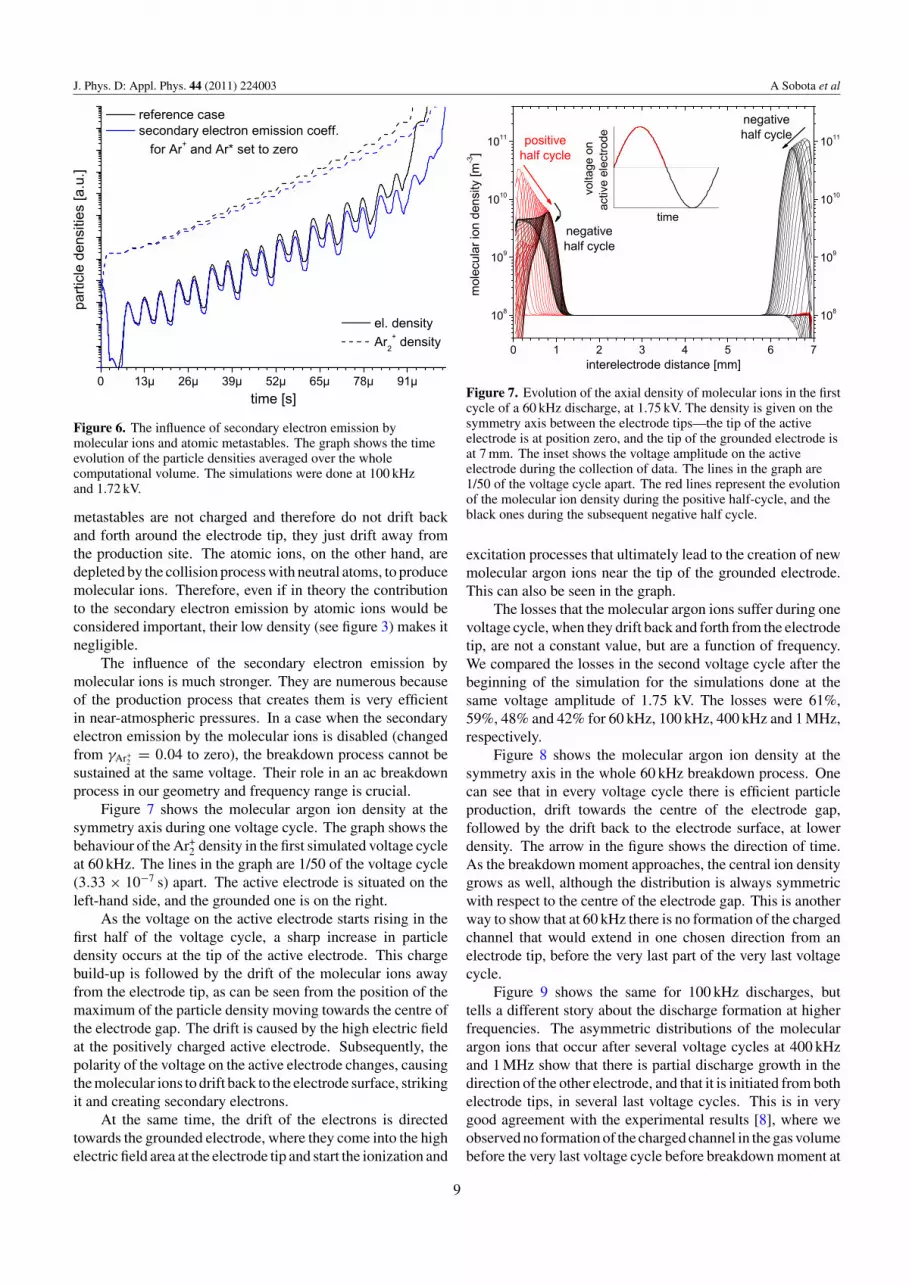
Figure 6. The influence of secondary electron emission bymolecular ions and atomic metastables. The graph shows the timeevolution of the particle densities averaged over the wholecomputational volume. The simulations were done at 100 kHzand 1.72 kV.

metastables are not charged and therefore do not drift backand forth around the electrode tip, they just drift away fromthe production site. The atomic ions, on the other hand, aredepleted by the collision process with neutral atoms, to producemolecular ions. Therefore, even if in theory the contributionto the secondary electron emission by atomic ions would beconsidered important, their low density (see figure 3) makes itnegligible.

The influence of the secondary electron emission bymolecular ions is much stronger. They are numerous becauseof the production process that creates them is very efficientin near-atmospheric pressures. In a case when the secondaryelectron emission by the molecular ions is disabled (changedfrom γAr+

2= 0.04 to zero), the breakdown process cannot be

sustained at the same voltage. Their role in an ac breakdownprocess in our geometry and frequency range is crucial.

Figure 7 shows the molecular argon ion density at thesymmetry axis during one voltage cycle. The graph shows thebehaviour of the Ar+

2 density in the first simulated voltage cycleat 60 kHz. The lines in the graph are 1/50 of the voltage cycle(3.33 × 10−7 s) apart. The active electrode is situated on theleft-hand side, and the grounded one is on the right.

As the voltage on the active electrode starts rising in thefirst half of the voltage cycle, a sharp increase in particledensity occurs at the tip of the active electrode. This chargebuild-up is followed by the drift of the molecular ions awayfrom the electrode tip, as can be seen from the position of themaximum of the particle density moving towards the centre ofthe electrode gap. The drift is caused by the high electric fieldat the positively charged active electrode. Subsequently, thepolarity of the voltage on the active electrode changes, causingthe molecular ions to drift back to the electrode surface, strikingit and creating secondary electrons.

At the same time, the drift of the electrons is directedtowards the grounded electrode, where they come into the highelectric field area at the electrode tip and start the ionization and

Figure 7. Evolution of the axial density of molecular ions in the firstcycle of a 60 kHz discharge, at 1.75 kV. The density is given on thesymmetry axis between the electrode tips—the tip of the activeelectrode is at position zero, and the tip of the grounded electrode isat 7 mm. The inset shows the voltage amplitude on the activeelectrode during the collection of data. The lines in the graph are1/50 of the voltage cycle apart. The red lines represent the evolutionof the molecular ion density during the positive half-cycle, and theblack ones during the subsequent negative half cycle.

excitation processes that ultimately lead to the creation of newmolecular argon ions near the tip of the grounded electrode.This can also be seen in the graph.

The losses that the molecular argon ions suffer during onevoltage cycle, when they drift back and forth from the electrodetip, are not a constant value, but are a function of frequency.We compared the losses in the second voltage cycle after thebeginning of the simulation for the simulations done at thesame voltage amplitude of 1.75 kV. The losses were 61%,59%, 48% and 42% for 60 kHz, 100 kHz, 400 kHz and 1 MHz,respectively.

Figure 8 shows the molecular argon ion density at thesymmetry axis in the whole 60 kHz breakdown process. Onecan see that in every voltage cycle there is efficient particleproduction, drift towards the centre of the electrode gap,followed by the drift back to the electrode surface, at lowerdensity. The arrow in the figure shows the direction of time.As the breakdown moment approaches, the central ion densitygrows as well, although the distribution is always symmetricwith respect to the centre of the electrode gap. This is anotherway to show that at 60 kHz there is no formation of the chargedchannel that would extend in one chosen direction from anelectrode tip, before the very last part of the very last voltagecycle.

Figure 9 shows the same for 100 kHz discharges, buttells a different story about the discharge formation at higherfrequencies. The asymmetric distributions of the molecularargon ions that occur after several voltage cycles at 400 kHzand 1 MHz show that there is partial discharge growth in thedirection of the other electrode, and that it is initiated from bothelectrode tips, in several last voltage cycles. This is in verygood agreement with the experimental results [8], where weobserved no formation of the charged channel in the gas volumebefore the very last voltage cycle before breakdown moment at

9

J. Phys. D: Appl. Phys. 44 (2011) 224003 A Sobota et al

Figure 8. Evolution of the axial density of the molecular ions in thewhole 60 kHz breakdown process, at 1.75 kV. The density is givenon the symmetry axis between the electrode tips—the tip of theactive electrode is at position zero, and the tip of the groundedelectrode is at 7 mm. The lines in the graph are 1/50 of the voltagecycle apart.

lower frequencies (60 to 220 kHz), but such observations weremade at higher frequencies (400 to 800 kHz).

The molecular ion densities are very low in the centralpart of the electrode gap for low frequencies—60 and 100 kHz,because the discharge does not partially propagate before thebridging of the electrode gap. When the gap is bridged,just before the breakdown moment, the central molecular iondensities rise to 1021 m−3, just like it can be seen in the profilesbelonging to the 400 kHz and 1 MHz simulations. The reasonwhy this happens earlier in the breakdown process in higherfrequencies is partial bridging of the gap during the voltagecycles before the last one, which can be seen also in theexperiments.

5. Discussion

In this paper we presented results of simulations in 0.7pure argon atmosphere using an ac driving voltage. Thesimulations were done using a two-dimensional fluid modeland a cylindrically symmetric geometry. The aim of this paperwas to give an overview of the most important characteristicsof the ac discharges in the frequency range where the dischargetakes more than a single cycle to form and the electron lossesare still drift dominated.

The model we used was adapted to describe theexperimental conditions which we gave an account of inthe accompanying paper [8]. The discharges in the givenexperimental conditions were gas volume discharges that grewin the space between the electrode tips, which made it possibleto model them in a 2D cylindrically symmetric geometry. Thesimulation results presented in this paper are in good agreementwith the experimentally observed data [8] in several importantrespects—the appearance of the discharge, its behaviour as afunction of frequency and the effect the change in frequencyhas on the minimum voltage needed for breakdown. Theresults presented in the previous section allowed us to explain

Figure 9. Evolution of the axial density of the molecular ions in thewhole breakdown process, at 1.75 kV, at 100 kHz, 400 kHz and1 MHz. The density is given on the symmetry axis between theelectrode tips—the tip of the active electrode is at position zero, andthe tip of the grounded electrode is at 7 mm. The lines in the graphsare 1/25 of voltage cycle apart: 0.4 µs at 100 kHz, 0.1 µs at 400 kHzand 0.04 µs at 1 MHz.

two phenomena that were thus far explained in a way that wasnot satisfactory in our experimental conditions or not explainedat all. These are presented in the following two subsections.

5.1. A lower threshold voltage for ac-driven discharges

The evolution of the particle densities takes multiple voltagecycles, which is essentially the reason why the ac-driven

10

J. Phys. D: Appl. Phys. 44 (2011) 224003 A Sobota et al

breakdown processes require a lower threshold voltage than thepulsed breakdown in the same experimental conditions. First,the discharge is allowed a longer time to form. It has beenshown many times that the formation time for the discharge isa steep function of the overvoltage used [10, 27], as the firstTownsend ionization coefficient is an exponential function ofthe applied electric field. From the experimental data [27] it canbe seen that the discharge formation time is a bijective functionof the overvoltage. If we make an additional assumptionthat the published data reflect a unique law that connects theformation time to the overvoltage, we are allowed to assumethe reverse function, one that would connect the overvoltage tothe discharge formation time. In this function, the overvoltagewould decrease as the formation time increased. From this,we can draw a conclusion that the more time we allow ourdischarge to form, the lower the voltage that we have to supply.This has already been shown in pulsed-voltage experiments bychanging the pulse slope [28]. Our ac discharges take as muchas three orders of magnitude longer to form, and therefore canbe expected to require a lower voltage.

Another, more important reason why the ac breakdownprocesses require a lower voltage than their pulsed equivalentsis that the voltage polarity changes while the dischargeforms, allowing for additional phenomena to help with thecharged particle production. The heavy charged species inac-driven breakdown processes drift back and forth around theelectrode tips, making the secondary electron emission fromelectrode surfaces an important source of electrons. In ourcase, the molecular ions are the key species responsible forthe secondary electron emission. This effect allows for aneffectively higher production of charged particles than is thecase in a unipolar fast discharge, even though the electronlosses in this frequency range are substantial. In pulseddischarges, secondary electron emission is not likely to playany role, because the heavy particles are effectively immobileduring the entire breakdown event. This has already beendemonstrated [20].

5.2. The lowering of the breakdown voltage with the increasein frequency

The experiments [8] have shown that the threshold voltageneeded for breakdown decreased with the increase infrequency. This phenomenon is also an effect replicated inthe simulations and it has not been previously explained in asatisfactory way, at least as far as our experimental conditionsare concerned. Two possible explanations were offered. First,there was a possibility that the electron drift losses werelowered with the increase in frequency [9]—we have alreadyshown in the accompanying paper [8] that the electron driftlosses were still very large in the whole frequency range weused, because the electron drift distance in one half of a voltagecycle was much larger than was the length of our electrode gap.There was certainly some lowering of the electron drift lossesover the entire frequency range we used, since it spread over1.5 orders of magnitude, but this effect alone cannot explainthe effects we have observed on its own. We do expect thelowering of the electron drift losses to become significant withfurther increase in the voltage frequency.

Second, a conjecture was made that due to the highelectron drift losses and low ion mobility, positive net chargewould form in the electrode gap away from the electrodes,modify the electric field and allow the starting of an avalancheprocess at lower voltages as the frequency increased [9]. Inour experimental and modelling conditions, we do not believethat this effect had a noteworthy influence on the dischargedevelopment. There are several reasons for this. One, we seethe lowering of the threshold voltage in the frequency rangebetween 60 and 220 kHz, as well as in higher frequencies. Thepeculiarity of this lower frequency range is that the formationof the channel to cross the electrode gap happens in one voltagecycle or less, and that the charged channel starts growing froman electrode tip. There is, therefore, no reason to assume‘islands’ of high charge density in the electrode gap away fromthe electrode tips, which would start avalanches somewhere inthe gas volume. The reason for the lowering of the breakdownvoltage must be something other than charge accumulation inthe electrode gap.

In addition, we have observed in the simulations thatthere really exists the threshold voltage under which theparticle densities do not rise, the particles do not multiplyand the breakdown can never occur, and that this voltageis a function of frequency. For example, a simulation of400 kHz or 1 MHz discharge will result in breakdown at voltageamplitude of 1.6 kV. The same voltage amplitude at 100 and60 kHz will not be sufficient for charge build-up and eventualbreakdown. We would like to focus on the beginning stagesof the simulations, where there is still no high particle densityof any species and the voltage has not gone through a phasecycle yet, making it impossible for the ions to drift back andforth in the electrode gap and create islands of high density.Even in these early stages in the simulations, there is a cleardifference between the discharges at different frequencies,where some will subsequently grow and develop at a givenvoltage amplitude, and some not. We do not believe thereason for this lies in the chemistry of the processes. At thesefrequencies, in a 0.7 bar argon atmosphere and a low ionizationdegree, the electron energy is given by and can follow thephase of the imposed electric field. Therefore, the electronenergy is independent of frequency at the start of the simulationin our frequency range, and the starting reaction rates in thesimulations are thus also independent of frequency.

The suggestion that the net charge build-up in theelectrode gap is responsible for the lowering of the thresholdvoltage as the voltage frequency increases is, thus, not asatisfactory explanation for our observations. Moreover, wewere experimenting and modelling a pin–pin electrode system.The net charge needed to modify the electric field already givenat the electrode tips is very high and can possibly be achievedvery late in the breakdown process, after the particle densitieshave sufficiently increased. This effect would possibly be ableto speed up the breakdown process long after it has alreadystarted, but not influence it from the beginning.

There is still an effect that causes the threshold voltageneeded for breakdown to drop with the increase in frequency.We believe that the solution to this problem lies in the behaviourof the molecular ions in a single voltage cycle. As shown in

11

J. Phys. D: Appl. Phys. 44 (2011) 224003 A Sobota et al

figures 7, 8 and 9, the molecular ion density oscillates back andforth around the electrode tip as the phase of the voltage on theactive electrode changes. In these oscillations, the molecularions undergo collisions with other species in the plasma andtheir density decreases as a result. The decrease in a singlevoltage cycle is a function of frequency, simply because inhigher frequencies there is less time available between theequivalent points in two subsequent voltage cycles for thecollisionally induced losses. Higher frequency, thus, meansless molecular ion losses, and higher density to drift back tothe electrode tip and induce secondary electron emission.

We have just explained how an increase in frequency cangive an effective increase in electron production. The loweringof the electron losses that are drift-dominated with the increasein frequency is not considered a noteworthy contribution, buteven if it were, this effect would add to the increase in thenet electron production in a single voltage cycle. The totalproduction rate of electrons can, therefore, be separated intwo parts—the part that is caused by the chemistry in thebreakdown process, and the part caused by the secondaryelectron emission. If we assume that at the threshold voltagefor the breakdown process one must have a certain constantminimum of the net electrons produced in a given time interval,and we know that the increase in frequency increases the partcaused by the secondary electron emission, it is clear that thepart caused by the chemistry can be lowered. The lowering ofthe contribution of the chemistry can be achieved by loweringof the mean electron energy via the imposed electric field. Thisis why breakdown processes at higher frequencies are possibleat lower voltages.

5.3. Outlook

We have shown that the simulations done on the HID lampsystem and 0.7 bar argon using ac voltage gave results that arein very good agreement with the experiments presented in theaccompanying paper [8]. There are, however, several ways inwhich the model we used can be improved. The size of thecomputational cells in the model is a concern. The geometryshould not be excessively coarse, because that would causeerrors in the calculations of various key parameters, such asthe electric fields in the system. On the other hand, very smallsize of computational cells would cause very long calculationtimes, especially at high frequencies. The implementation ofthe local grid refinement would greatly help this issue.

Additionally, the chemistry used in the model may not besufficiently complex for the description of a breakdown processin near-atmospheric pressure. A possible improvement wouldbe the addition of another effective atomic metastable state thatwould represent the 4p and higher lying excited states in theargon atom. Excimer molecules could be added as well. Thiswould give a more correct effect of the excited species on thebreakdown process.

6. Conclusion

This paper has shown the results of two-dimensional fluidmodel simulations of ac breakdown in a 0.7 bar argon

atmosphere. We have used a two-pin electrode systemenclosed in an HID lamp geometry with fixed length (7 mm)of the electrode gap. With the electrode gap and the gaspressure fixed, we were able to distill the effect of the voltagefrequency (60 kHz to 1 MHz) in the overall breakdown process.We have shown its effect on the appearance of the discharge,the threshold voltage needed for breakdown and the timing ofthe breakdown process. The results of the simulations are ingood agreement with the experimental data [8], both in theirqualitative behaviour as a function of frequency, as in theirquantitative behaviour in terms of breakdown voltages andformative times. We have also demonstrated the importanceof the secondary electron emission from electrode surfaces, inparticular by molecular ions, in the breakdown process andlinked it to the lowering of the threshold voltage with theincrease in frequency observed both in experiment and model.

Acknowledgments

This work was supported by Philips Lighting.

References

[1] Pfeiffer W 1991 High-frequency voltage stress of insulation.Methods of testing IEEE Trans. Electr. Insul. 26 239–46

[2] Koppisetty K and Kirkici H 2008 Breakdown characteristics ofhelium and nitrogen at kHz frequency range in partialvacuum for point-to-point electrode configuration IEEETrans. Dielectr. Electr. Insul. 15 749–55

[3] Park J, Henins I, Herrmann H W and Selwyn G S 2001 Gasbreakdown in an atmospheric pressure radio-frequencycapacitive plasma source J. Appl. Phys. 89 15–9

[4] Shi J J and Kong M G 2005 Large-volume and low-frequencyatmospheric glow discharges without dielectric barrierAppl. Phys. Lett. 86 091502

[5] Walsh J L, Zhang Y T, Iza F and Kong M G 2008Atmospheric-pressure gas breakdown from 2 to 100 MHzAppl. Phys. Lett. 93 221505

[6] Sießegger B, Guldner H and Hirschmann G 2005 Ignitionconcepts for high frequency operated HID lamps Proc. 36thIEEE Power Electronics Specialists Conf. pp 1500–6

[7] Beckers J, Manders F, Aben P C H, Stoffels W W andHaverlag M 2008 Pulse, dc and ac breakdown in highpressure gas discharge lamps J. Phys. D: Appl. Phys.41 144028

[8] Sobota A, Kanters J H M, Manders F, Gendre M F, Hendriks J,van Veldhuizen E M and Haverlag M 2011 AC breakdownin near-atmospheric pressure noble gases: I. ExperimentJ. Phys. D.: Appl. Phys. 44 224002

[9] Meek J M and Craggs J D 1953 Electrical Breakdown ofGases (Oxford: Oxford University Press)

[10] Raizer Yu P 1991 Gas Discharge Physics (Berlin: Springer)[11] Brown S C 1961 Basic Data of Plasma Physics (Cambridge,

MA: MIT Press)[12] Ardenne M V 1962 Tabellen zur Angewandten Physik I

(Berlin: VEB Deutscher Verlag der Wissenschften)[13] Grigoriev I S and Meilikhov E Z 1997 Hanbook of Physical

Quantities (Boca Raton, FL: CRC Press)[14] Brok W J M 2005 Modelling of transient phenomena in gas

discharges PhD Thesis Technische Universiteit Eindhoven[15] Hagelaar G J M and Pitchford L C 2005 Solving the

boltzmann equation to obtain electron transport coefficientsand rate coefficients for fluid models Plasma Sources Sci.Technol. 14 722–33

12

J. Phys. D: Appl. Phys. 44 (2011) 224003 A Sobota et al

[16] Balcon N, Hagelaar G J M and Boeuf J P 2008 Numericalmodel of an argon atmospheric pressure RF discharge IEEETrans. Plasma Sci. 36 2782–7

[17] Klucharev A N and Vujnovic V 1990 Chemi-ionization inthermal-energy binary collisions of optically excited atomsPhys. Rep. 185 55–81

[18] Bogaerts A and Gijbels R 2002 Hybrid modelling network forhelium-argon-copper hollow cathode discharge used forlaser applications J. Appl. Phys. 92 6408–22

[19] Jonkers J 1998 Excitation and transport in small scaleplasmas PhD Thesis Technische UniversiteitEindhoven

[20] Sobota A, Manders F, van Veldhuizen E M, van Dijk J andHaverlag M 2010 The role of metastables in the formationof an argon discharge in a two-pin geometry IEEE Trans.Plasma Sci. 38 2289–99

[21] van Dijk J, Peerenboom K, Jimenez M, Mihailova D andvan der Mullen J 2009 The plasma modelling toolkitplasimo J. Phys. D: Appl. Phys. 42 194012

[22] Hagelaar G J M and Kroesen G M W 2000 Modeling ofmicrodischarges in plasma addressed liquid crystaldisplays J. Appl. Phys. 88 2252–62

[23] Hagelaar G J M, de Hoog F J and Kroesen G M W 2000Boundary conditions in fluid models of gas dischargesPhys. Rev. E 62 2252–62

[24] Brok W J M, van Dijk J, Bowden M D, van der Mullen J J A Mand Kroesen G M W 2003 A model study of propagation ofthe first ionization wave during breakdown in a straight tubecontaining argon J. Phys. D: Appl. Phys. 36 1967–79

[25] Brok W J M, Gendre M F, Haverlag M andvan der Mullen J J A M 2007 Numerical description of highfrequency ignition of fluorescent tubes J. Phys. D: Appl.Phys. 40 3931–6

[26] Ellis H W, Pai R Y, McDaniel E W, Mason E A andViehland L A 1976 Transport properties of gaseous ionsover a wide energy range At. Data Nucl. Data Tables17 177–210

[27] Moss R A, Eden J G and Kushner M J 2004 Avalanche processin an idealized lamp: I. Measurements of formativebreakdown time J. Phys. D: Appl. Phys. 37 2502–9

[28] Sobota A, Lebouvier A, Kramer N J, van Veldhuizen E M,Stoffels W W, Manders F and Haverlag M 2009 Speed ofstreamers in argon over a flat surface of a dielectric J. Phys.D: Appl. Phys. 42 015211

13