Embed Size (px)
Citation preview
San Jose State University San Jose State University
SJSU ScholarWorks SJSU ScholarWorks
Mineta Transportation Institute Publications
12-2021
Achieving Excellence for California’s Freight System: Developing Achieving Excellence for California’s Freight System: Developing
Competitiveness and Performance Metrics; Incorporating Competitiveness and Performance Metrics; Incorporating
Sustainability, Resilience, and Workforce Development Sustainability, Resilience, and Workforce Development
Jian-yu Ke California State University, Dominguez Hills
Fynnwin Prager California State University, Dominguez Hills
Jose Martinez California State University, Dominguez Hills
Chris Cagle Mineta Transportation Institute
Follow this and additional works at: https://scholarworks.sjsu.edu/mti_publications
Part of the Operations and Supply Chain Management Commons, Strategic Management Policy
Commons, and the Transportation Commons
Recommended Citation Recommended Citation Jian-yu Ke, Fynnwin Prager, Jose Martinez, and Chris Cagle. "Achieving Excellence for California’s Freight System: Developing Competitiveness and Performance Metrics; Incorporating Sustainability, Resilience, and Workforce Development" Mineta Transportation Institute Publications (2021). https://doi.org/10.31979/mti.2021.2023
This Report is brought to you for free and open access by SJSU ScholarWorks. It has been accepted for inclusion in Mineta Transportation Institute Publications by an authorized administrator of SJSU ScholarWorks. For more information, please contact [email protected].
Project 2023 November 2021
S. TSU SAN JOSE STATE 'J UNIVERSITY
C':).. California State University Q Transportation Consortium
1MINETA TRANSPORTATION
INSTITUTE
CALIFORNIA STATE UNIVERSITY LONG BEACH
Achieving Excellence for California’s Freight System: Developing Competitiveness and Performance Metrics; Incorporating Sustainability, Resilience, and Workforce Development
Jian-yu Ke, PhD Jose N. Martinez, PhD Fynnwin Prager, PhD Chris Cagle
C S U T R A N S P O R T A T I O N C O N S O R T I U M transweb.sjsu.edu/csutc
__________________________________________________________________________________
Mineta Transportation Institute Founded in 1991, the Mineta Transportation Institute (MTI), an organized research and training unitin partnership with the Lucas College and Graduate School of Business at San José State University (SJSU), increases mobility for all by improving the safety, efficiency, accessibility, and convenience of our nation’s transportation system. Through research, education, workforce development, and technology transfer, we help create a connected world. MTI leads the Mineta Consortium for Transportation Mobility (MCTM) funded by the U.S. Department of Transportation and the California State University Transportation Consortium (CSUTC) funded by the State of California through Senate Bill 1. MTI focuses on three primary responsibilities:
Research Master of Science in Transportation Management, plus graduate certificates that
MTI conducts multi-disciplinary research include High-Speed and Intercity Rail focused on surface transportation that Management and Transportation Security contributes to effective decision making. Management. These flexible programs offer Research areas include: active transportation; live online classes so that working planning and policy; security and transportation professionals can pursue an counterterrorism; sustainable transportation advanced degree regardless of their location. and land use; transit and passenger rail; transportation engineering; transportation Information and Technology Transfer finance; transportation technology; and workforce and labor. MTI research MTI utilizes a diverse array of dissemination publications undergo expert peer review to methods and media to ensure research results ensure the quality of the research. reach those responsible for managing change.
These methods include publication, seminars, Education and Workforce workshops, websites, social media, webinars,
and other technology transfer mechanisms. To ensure the efficient movement of people and Additionally, MTI promotes the availability of products, we must prepare a new cohort of completed research to professional transportation professionals who are ready to organizations and works to integrate the lead a more diverse, inclusive, and equitable research findings into the graduate education transportation industry. To help achieve this, program. MTI’s extensive collection of MTI sponsors a suite of workforce transportation-related publications is development and education opportunities. The integrated into San José State University’s Institute supports educational programs offered world-class Martin Luther King, Jr. Library. by the Lucas Graduate School of Business: a
Disclaimer
The contents of this report reflect the views of the authors, who are responsible for the facts and accuracyof the information presented herein. This document is disseminated in the interest of information exchange. MTI’s research is funded, partially or entirely, by grants from the California Department of Transportation, the California State University Office of the Chancellor, the U.S. Department of Homeland Security, and the U.S. Department of Transportation, who assume no liability for the contents or use thereof. This report does not constitute a standard specification, design standard, or regulation.
Report 21-28
Achieving Excellence for California’s Freight System: Developing Competitiveness and
Performance Metrics; Incorporating Sustainability, Resilience, and Workforce
Development
Jian-yu Ke, PhD Fynnwin Prager, PhD Jose N. Martinez, PhD
Chris Cagle
November 2021
A publication of the Mineta Transportation Institute
Created by Congress in 1991
College of Business San José State University
San José, CA 95192-0219
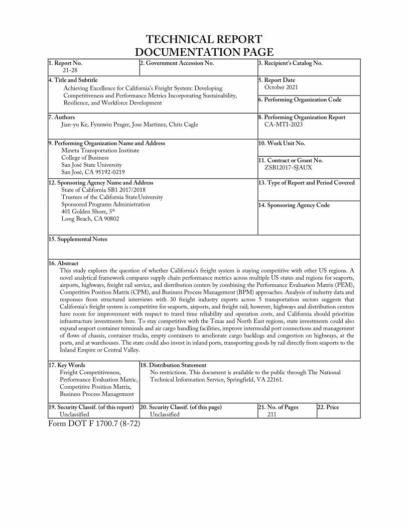
TECHNICAL REPORT DOCUMENTATION PAGE
1. Report No. 21-28
2. Government Accession No. 3. Recipient’s Catalog No.
4. Title and Subtitle Achieving Excellence for California’s Freight System: Developing Competitiveness and Performance Metrics Incorporating Sustainability, Resilience, and Workforce Development
5. Report Date October 2021
6. Performing Organization Code
7. Authors Jian-yu Ke, Fynnwin Prager, Jose Martinez, Chris Cagle
8. Performing Organization Report CA-MTI-2023
9. Performing Organization Name and Address Mineta Transportation Institute College of Business San José State University San José, CA 95192-0219
10. Work Unit No.
11. Contract or Grant No. ZSB12017-SJAUX
12. Sponsoring Agency Name and Address State of California SB1 2017/2018 Trustees of the California State University Sponsored Programs Administration 401 Golden Shore, 5th Long Beach, CA 90802
13. Type of Report and Period Covered
14. Sponsoring Agency Code
15. Supplemental Notes
16. Abstract This study explores the question of whether California's freight system is staying competitive with other US regions. A novel analytical framework compares supply chain performance metrics across multiple US states and regions for seaports, airports, highways, freight rail service, and distribution centers by combining the Performance Evaluation Matrix (PEM), Competitive Position Matrix (CPM), and Business Process Management (BPM) approaches. Analysis of industry data and responses from structured interviews with 30 freight industry experts across 5 transportation sectors suggests that California's freight system is competitive for seaports, airports, and freight rail; however, highways and distribution centers have room for improvement with respect to travel time reliability and operation costs, and California should prioritize infrastructure investments here. To stay competitive with the Texas and North East regions, state investments could also expand seaport container terminals and air cargo handling facilities, improve intermodal port connections and management of flows of chassis, container trucks, empty containers to ameliorate cargo backlogs and congestion on highways, at the ports, and at warehouses. The state could also invest in inland ports, transporting goods by rail directly from seaports to the Inland Empire or Central Valley.
17. Key Words Freight Competitiveness, Performance Evaluation Matric, Competitive Position Matrix, Business Process Management
18. Distribution Statement No restrictions. This document is available to the public through The National Technical Information Service, Springfield, VA 22161.
19. Security Classif. (of this report) Unclassified
20. Security Classif. (of this page) Unclassified
21. No. of Pages 211
22. Price
Form DOT F 1700.7 (8-72)
Copyright © 2021
by Mineta Transportation Institute
All rights reserved.
DOI: 10.31979/mti.2021.2023
Mineta Transportation Institute College of Business
San José State University San José, CA 95192-0219
Tel: (408) 924-7560 Fax: (408) 924-7565
Email: [email protected]
transweb.sjsu.edu/research/2023
ACKNOWLEDGMENTS The California State University Transportation Center at San Jose State University provided funding for this study. The authors are thankful for research assistance from Levicent Mira and Matthew Taylor. The authors also very much appreciate feedback and support from Gillian Fischer, Chandra Khan, Brigette Brown, Garth Hopkins, Fran Inman, Laura Pennebaker, Tom O'Brien, Genevieve Giuliano, Jeffrey Morneau, Nieves Castro, Yatman Kwan, Akiko Yamagami, David Gamboa, Felicia Hernandez, Mishan Montgomery, and Nicholas Little. Special thanks to Executive Director Jan Vogel of the South Bay Workforce Investment Board, and Deborah Shepard and Amelia Klawon for their support and contributions to this study. However, any opinions, findings, conclusions, or recommendations in this document are those of the authors and do not necessarily reflect the views of their respective organizations.
M I N E T A T R A N S P O R T A T I O N I N S T I T U T E iv
CONTENTS Acknowledgments ................................................................................................................ iv List of Figures........................................................................................................................ ix List of Tables......................................................................................................................... xi Executive Summary ...............................................................................................................1 1. Introduction.....................................................................................................................2 2. Literature Review.............................................................................................................3 3. Methodology ...................................................................................................................5
3.1 Questionnaire Design .............................................................................................5 3.2 Profile of Experts Interviewed.................................................................................5 3.3 The PEM and CPM Approaches ...........................................................................7 3.4 The BPM Approach...............................................................................................9
4. Competitiveness of the Freight System from the SCM’s Perspective................................11 5. Seaports............................................................................................................................15
5.1 Introduction............................................................................................................15 5.2 Literature Review ...................................................................................................21 5.3 PEM and CPM Analyses .......................................................................................24
5.3.1 Data.............................................................................................................24 5.3.2 PEM Analysis..............................................................................................30 5.3.3 CPM Analysis .............................................................................................31
5.4 BPM Analysis.........................................................................................................35 5.5 Comments from Interviews.....................................................................................39
5.5.1 Data and measures .......................................................................................39 5.5.2 Current state of California freight competitiveness ......................................40 5.5.3 The future of California freight competitiveness ..........................................41
5.6 Port Performance with respect to the Environment, Sustainability, and Resilience.........................................................................................................42
5.7 Conclusion..............................................................................................................43 5.7.1 Findings.......................................................................................................43 5.7.2 Suggestions..................................................................................................43 5.7.3 Workforce Development Plan .....................................................................44
6. Airports............................................................................................................................45 6.1 Introduction............................................................................................................45 6.2 Literature Review ...................................................................................................50
M I N E T A T R A N S P O R T A T I O N I N S T I T U T E
6.3 PEM and CPM Analyses .......................................................................................52 6.3.1 Data.............................................................................................................52 6.3.2 PEM Analysis..............................................................................................57 6.3.3 CPM Analysis .............................................................................................58
6.4 BPM Analysis.........................................................................................................61 6.5 Comments from Interviews.....................................................................................63
6.5.1 Data and measures .......................................................................................63 6.5.2 Current State of California freight competitiveness......................................63 6.5.3 The future of California’s freight competitiveness ........................................64
6.6 Port Performance with respect to the Environment, Sustainability, and Resilience.........................................................................................................64
6.7 Conclusion..............................................................................................................65 6.7.1 Findings ......................................................................................................65 6.7.2 Suggestions .................................................................................................65 6.7.3 Workforce Development Plan......................................................................66
7. Highways.........................................................................................................................67 7.1 Introduction............................................................................................................67 7.2 Literature Review ...................................................................................................69 7.3 PEM and CPM Analyses .......................................................................................75
7.3.1 PEM Analysis .............................................................................................79 7.3.2 CPM Analysis .............................................................................................79
7.4 BPM Analysis.........................................................................................................82 7.5 Summary of Open-Ended Questions......................................................................83
7.5.1 Current state of California freight competitiveness ......................................84 7.5.2 The future of California freight competitiveness ..........................................84
7.6 Highway Performance with respect to the Environment, Sustainability, and Resilience ..................................................................................85
7.7 Conclusions ............................................................................................................85 7.7.1 Findings.......................................................................................................85 7.7.2 Suggestions..................................................................................................85 7.7.3 Workforce Development Plan......................................................................86
8. Freight Rails.....................................................................................................................87 8.1 Introduction............................................................................................................87 8.2 Literature review.....................................................................................................95 8.3 PEM and CPM Analysis........................................................................................95
M I N E T A T R A N S P O R T A T I O N I N S T I T U T E
8.3.1 Regional Comparison ..................................................................................96 8.3.2 PEM Analysis..............................................................................................99 8.3.3 CPM Analyses.............................................................................................101
8.4 BPM Analysis ........................................................................................................104 8.5 Discussion of interviewee responses to open-ended questions ................................105
8.5.1 Data and measures .......................................................................................105 8.5.2 Current state of California freight competitiveness ......................................106 8.5.3 The future of California freight rail competitiveness ....................................107 8.5.4 Freight Rail Performance with respect to the Environment,
Sustainability, and Resilience .......................................................................109 8.6 Conclusion..............................................................................................................109
8.6.1 Findings.......................................................................................................110 8.6.2 Suggestions..................................................................................................111 8.6.3 Workforce Development Plan......................................................................111
9. Distribution Centers........................................................................................................112 9.1 Introduction............................................................................................................112 9.2 Literature Review ..................................................................................................120 9.3 PEM and CPM Analyses ......................................................................................122
9.3.1 Data ............................................................................................................122 9.3.2 PEM Analysis .............................................................................................127 9.3.3 CPM Analysis ............................................................................................128
9.4 BPM Analysis.........................................................................................................131 9.5 Comments from Interviews.....................................................................................134
9.5.1 Data and measures .......................................................................................134 9.5.2 Current state of California freight competitiveness .....................................134 9.5.3 The future of California freight competitiveness ..........................................135
9.6 Distribution Center Performance with respect to the Environment, Sustainability, and Resilience ..................................................................................136
9.7 Conclusion..............................................................................................................136 9.7.1 Findings.......................................................................................................136 9.7.2 Suggestions..................................................................................................137 9.7.3 Workforce Development Plan......................................................................137
10. Public Policy......................................................................................................................139 10.1 2020 California Freight Mobility Plan ....................................................................139 10.2 2018 California State Rail Plan...............................................................................142
M I N E T A T R A N S P O R T A T I O N I N S T I T U T E
10.3 2021 Infrastructure and American Jobs Act ............................................................143 11. Summary and Conclusions...............................................................................................145
11.1 Overall Competitiveness Scores ..............................................................................145 11.2 Suggested Priorities for Investments ......................................................................147 11.3 Workforce Development Plans ..............................................................................148 11.4 Limitations ............................................................................................................149
Appendix A Questionnaire for Seaport .................................................................................151 Appendix B Questionnaire for Airport...................................................................................159 Appendix C Questionnaire for Highway ...............................................................................167 Appendix D Questionnaire for Freight Rail...........................................................................174 Appendix E Questionnaire for Distribution Center ............................................................... 180 Bibliography ........................................................................................................................... 187 About the Authors.................................................................................................................. 195
M I N E T A T R A N S P O R T A T I O N I N S T I T U T E
LIST OF FIGURES Figure 1. Performance Evaluation Matrix (PEM)..................................................................7 Figure 2. Competitive Position Matrix (CPM) ......................................................................8 Figure 3. Eight-step Business Process Management Approach..............................................10 Figure 4. Contributions of Freight Sectors on Supply Chain Performances............................13 Figure 5. Trend of Import Shares of Containerized Vessel Tonnage during 2006-2020.........18 Figure 6. Canadian Port-Railroad Connections .....................................................................20 Figure 7. Growing Competition among Canals .....................................................................21 Figure 8. PEM for Port of Los Angels...................................................................................31 Figure 9. CPM for Port of Los Angeles versus New York/Newark ........................................32 Figure 10. CPM for Port of Los Angeles versus Seattle .........................................................32 Figure 11. CPM for Port of Los Angeles versus Houston ......................................................34 Figure 12. CPM for Port of Los Angeles versus Savannah.....................................................35 Figure 13. Trend of Import Shares of Air Freight Tonnage during 2006-2020 ......................47 Figure 14. Inland Port Connections.......................................................................................48 Figure 15. ORD Northeast Cargo Three-Phase Development ..............................................48 Figure 16. PEM for LAX Airport..........................................................................................58 Figure 17. CPM for LAX versus ORD..................................................................................58 Figure 18. CPM for LAX versus DFW .................................................................................59 Figure 19. CPM for LAX versus IAH ...................................................................................59 Figure 20. CPM for LAX versus JFK ....................................................................................60 Figure 21. CPM for LAX versus ATL...................................................................................60 Figure 22. FHWA National Highway System, 2017 .............................................................67 Figure 23. California Freight Network: California Mobility Plan 2020..................................68 Figure 24. PEM for California – Highway.............................................................................79 Figure 25. CPM for California and Arizona ..........................................................................80 Figure 26. CPM for California and Texas..............................................................................81 Figure 27. CPM for California and New Mexico...................................................................81 Figure 28. Class 1 and Public Agency Owned Rail System in California................................88 Figure 29. US Freight Networks by Transportation Mode.....................................................89 Figure 30. PEM Diagram for California................................................................................101 Figure 31. CPM Diagram Comparing California and Washington .......................................102 Figure 32. CPM Diagram Comparing California and Texas..................................................103 Figure 33. CPM Diagram Comparing California and Georgia ..............................................103
M I N E T A T R A N S P O R T A T I O N I N S T I T U T E ix
Figure 34. CPM Diagram Comparing California and New York...........................................104 Figure 35. CPM Diagram Comparing California and Pennsylvania.......................................104 Figure 36. Population Growth of U.S Major Cities during 2005–2019..................................115 Figure 37. PEM for Los Angeles ...........................................................................................128 Figure 38. CPM for L.A. versus Tampa, FL..........................................................................128 Figure 39. CPM for L.A. versus Houston, TX ......................................................................129 Figure 40. CPM for L.A. versus Atlanta, GA........................................................................129 Figure 41. CPM for L.A. versus Newark, NJ.........................................................................130 Figure 42. CPM for L.A. versus Seattle, WA ........................................................................130 Figure 43. CPM for L.A. versus Phoenix, AZ .......................................................................131 Figure 44. CPM for L.A. versus Las Vegas, NV....................................................................131 Figure 45. Scorecard of Freight Competitiveness ...................................................................147
M I N E T A T R A N S P O R T A T I O N I N S T I T U T E x
LIST OF TABLES Table 1. Profile of Experts Interviewed..................................................................................6 Table 2. Steps for PEM and CPM ........................................................................................7 Table 3. SCOR Performance Attributes ................................................................................12 Table 4. Contributions and Weights of Freight Sectors .........................................................14 Table 5. Import Shares of Containerized Vessel Tonnage in 2020 .........................................16 Table 6. Import Shares of Containerized Vessel Tonnage from 2006–2020...........................17 Table 7. Growth of Containerized Vessel Tonnage from 2006–2020.....................................19 Table 8. Key Drivers of Port Competitiveness .......................................................................22 Table 9. Performance Measures foe the Key Drivers of Port Competitiveness .......................23 Table 10. Data for the Port Performance Measures ...............................................................26 Table 11. Importance and Percentiles of the Port Performance Measures ..............................28 Table 12. Ranking of Top 20 U.S. Ports................................................................................30 Table 13. Percentiles in the Performances of Port of L.A. and Benchmarking Ports ..............36 Table 14. Benchmark Scores—Seaport ..................................................................................38 Table 15. Import Shares by Air Freight Tonnage in 2020......................................................45 Table 16. Import Shares of Air Freight Tonnage during 2006–2020......................................46 Table 17. Growth of Air Freight Tonnage during 2006–2020 ...............................................46 Table 18. Key Drivers and Performance Measures of Airport Competitiveness......................50 Table 19. Performance Measures for the Key Drivers of Port Competitiveness......................51 Table 20. Data for the Airport Performance Measures...........................................................53 Table 21. Importance and Percentiles of the Airport Performance Measures .........................55 Table 22. Ranking of U.S. Airport Competitiveness ..............................................................57 Table 23. Percentiles in the Performances of LAX Airport and Benchmarking Airports........61 Table 24. Benchmark Scores - Airport...................................................................................62 Table 25. Freight Performance Measure Primer for Highway Systems ..................................70 Table 26. Survey Key Drivers and Importance for Competitiveness .......................................72 Table 27. Performance Measures Data Collected...................................................................73 Table 28. Highway Performance Measures Importance and Percentile Ranks........................76 Table 29. Percentiles Performances of California’s Highway System and
Benchmarking States. ............................................................................................82 Table 30. Benchmarking Scores.............................................................................................83 Table 31. Rail Performance Metrics by Company..................................................................92 Table 32. Major Terminal Dwell Times by Region and Company, 2020 ...............................93
M I N E T A T R A N S P O R T A T I O N I N S T I T U T E xi
Table 33. Key Drivers of Rail Freight Competitiveness..........................................................95 Table 34. California Freight Rail Operations and Traffic.......................................................97 Table 35. Southwest States Freight Rail Operations and Traffic............................................97 Table 36. Pacific Northwest States Freight Rail Operations and Traffic ................................97 Table 37. Texas and South Central States Freight Rail Operations and Traffic .....................99 Table 38. Southeast and South Atlantic States Freight Rail Operations and Traffic ..............99 Table 39. Northeast States Freight Rail Operations and Traffic.............................................100 Table 40. Importance and Percentiles of the Rail Freight Performance Measures ..................101 Table 41. Importance and Relative Performance of Rail Freight Across States ......................102 Table 42. BPM Analysis Comparison of California with Other Competitor States ...............105 Table 43. 2005–2019 Annual Growth Rate and Share of Real GDP, Population, and
Employment—Top 25 U.S. Metropolitan areas.....................................................113 Table 44. 2005–2019 Annual Growth Rate and Share of Real GDP, Population, and
Employment—Top 10 California Metropolitan areas ............................................116 Table 45. Summary of Amazon Fulfillment Centers in the U.S. ............................................118 Table 46. List of Amazon’s Fulfillment Centers in California................................................119 Table 47. Key Drivers of Distribution Center’s Location Selection ........................................120 Table 48. Performance Measures for the Key Drivers of Distribution Center’s
Location Selection .................................................................................................121 Table 49. Data for the Distribution Center Performance Measures .......................................123 Table 50. Importance and Percentiles of the Distribution Center Performance Measures ......125 Table 51. Ranking of U.S. City Competitiveness...................................................................127 Table 52. Percentiles in the Performances of Los Angeles and Benchmarking Cities .............132 Table 53. Benchmark Scores—Distribution Center ...............................................................133 Table 54. Overall Competitiveness Scores of California and Competing States .....................146 Table 55. Suggested Priorities for Investments........................................................................148
M I N E T A T R A N S P O R T A T I O N I N S T I T U T E xii
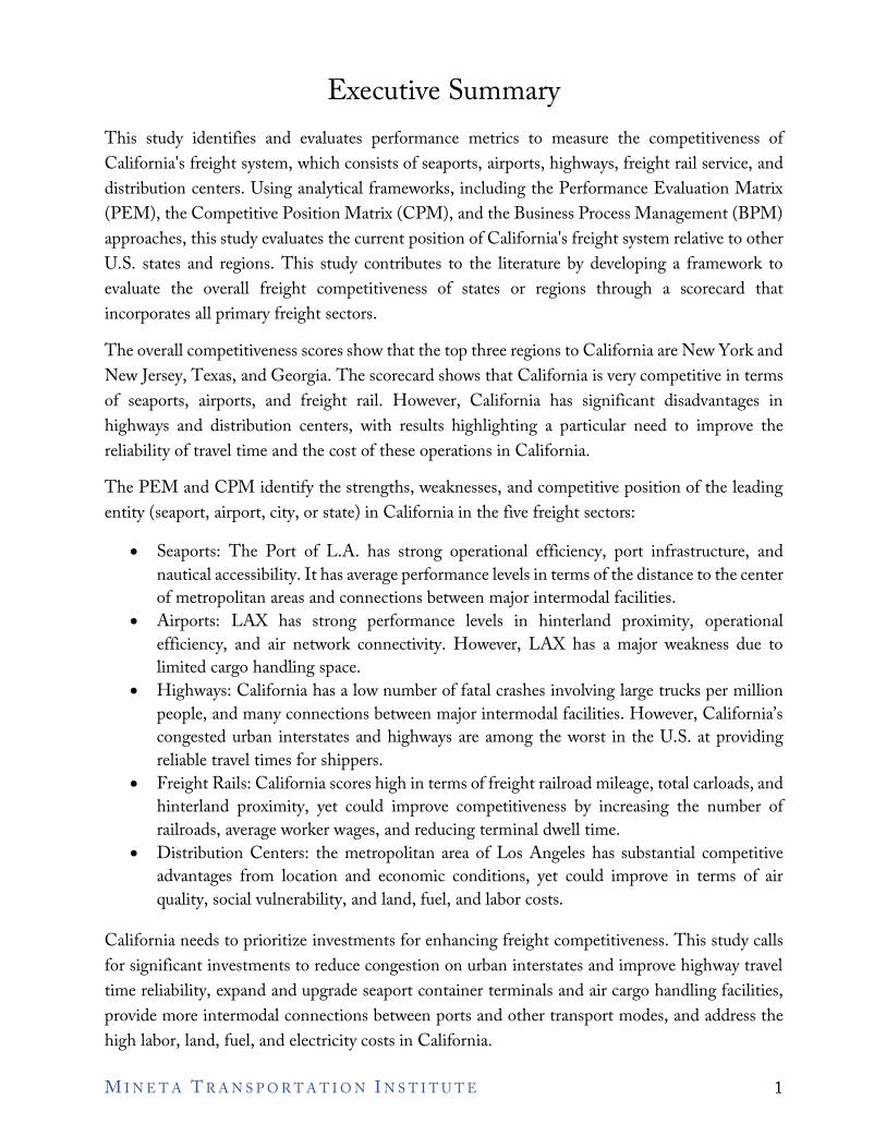
Executive Summary This study identifies and evaluates performance metrics to measure the competitiveness of California's freight system, which consists of seaports, airports, highways, freight rail service, and distribution centers. Using analytical frameworks, including the Performance Evaluation Matrix (PEM), the Competitive Position Matrix (CPM), and the Business Process Management (BPM) approaches, this study evaluates the current position of California's freight system relative to other U.S. states and regions. This study contributes to the literature by developing a framework to evaluate the overall freight competitiveness of states or regions through a scorecard that incorporates all primary freight sectors. The overall competitiveness scores show that the top three regions to California are New York and New Jersey, Texas, and Georgia. The scorecard shows that California is very competitive in terms of seaports, airports, and freight rail. However, California has significant disadvantages in highways and distribution centers, with results highlighting a particular need to improve the reliability of travel time and the cost of these operations in California. The PEM and CPM identify the strengths, weaknesses, and competitive position of the leading entity (seaport, airport, city, or state) in California in the five freight sectors:
• Seaports: The Port of L.A. has strong operational efficiency, port infrastructure, and nautical accessibility. It has average performance levels in terms of the distance to the center of metropolitan areas and connections between major intermodal facilities.
• Airports: LAX has strong performance levels in hinterland proximity, operational efficiency, and air network connectivity. However, LAX has a major weakness due to limited cargo handling space.
• Highways: California has a low number of fatal crashes involving large trucks per million people, and many connections between major intermodal facilities. However, California’s congested urban interstates and highways are among the worst in the U.S. at providing reliable travel times for shippers.
• Freight Rails: California scores high in terms of freight railroad mileage, total carloads, and hinterland proximity, yet could improve competitiveness by increasing the number of railroads, average worker wages, and reducing terminal dwell time.
• Distribution Centers: the metropolitan area of Los Angeles has substantial competitive advantages from location and economic conditions, yet could improve in terms of air quality, social vulnerability, and land, fuel, and labor costs.
California needs to prioritize investments for enhancing freight competitiveness. This study calls for significant investments to reduce congestion on urban interstates and improve highway travel time reliability, expand and upgrade seaport container terminals and air cargo handling facilities, provide more intermodal connections between ports and other transport modes, and address the high labor, land, fuel, and electricity costs in California.
M I N E T A T R A N S P O R T A T I O N I N S T I T U T E 1
1. Introduction The Governor’s Executive Order (EO) B-32-15, signed in July 2015, identified the economic impact of freight on California, and required the development of the California Sustainable Freight Action Plan (CSFAP). The CSFAP, which was completed in July 2016, established clear targets to improve freight efficiency, transition to zero-emission technologies, and increase the competitiveness of California's freight system. This study aims to define what a competitive freight system would be and measure the competitiveness of California’s freight system. The 2020 California Freight Mobility Plan states that “the role of freight transportation in economic competitiveness is usually assumed to be a function of freight system capacity, performance, and efficiency” (Newsom, Kim, and Omishakin 2019, 31). The literature proposes several performance metrics related to freight system capacity, performance, and efficiency (NASEM 2011; Yeo, Roe, and Dinwoodie 2008, 2011; Verhetsel and Sel 2009; Notteboom and Yap 2012; Giuliano and O’Brien 2016; Parola et al. 2017; Easley et al. 2017; Giuliano 2017; Chambers et al. 2018; Giuliano and Hassan 2018, 2019). For example, the METRANS Transportation Center defines economic competitiveness and the freight sector and proposes a framework for developing measures for the CSFAP (Giuliano 2017; Giuliano and Hassan 2018, 2019). They propose several metrics to measure financial performance, workforce performance, and overall economic performance across states. This study identifies the performance metrics contributing to a competitive freight system, consisting of seaports, airports, highways, freight rails, and distribution centers. Using analytical frameworks including the Performance Evaluation Matrix (PEM) and the Competitive Position Matrix (CPM) approaches developed by Lambert and Sharma (1990) and the Business Process Management (BPM) approach proposed by Su and Ke (2017), this study evaluates the current position of California’s freight system as compared with other states. This study contributes to the literature by developing a framework to evaluate competitiveness through a scorecard consisting of primary freight sectors. It highlights the importance of infrastructure, bottlenecks, and workforce development issues, and provides policy recommendations to increase the competitiveness of California’s freight system. We organize the remainder of the report as follows. Section 2 surveys the extant literature. Section 3 introduces the research methodology. Section 4 interprets the competitiveness of the freight system from the supply chain management (SCM)'s perspective. In Sections 5, 6, 7, 8, and 9, we report the findings for each of the five freight sectors: seaports, airports, highways, freight rails, and distribution centers. Section 10 analyzes the public policies that contribute to the competitiveness of California’s freight system. Section 11 concludes the study with a comprehensive analysis of California’s competitive position with competing states.
M I N E T A T R A N S P O R T A T I O N I N S T I T U T E 2
2. Literature Review This study involves several research streams, including freight competitiveness and performance measurements of seaports, airports, highways, freight rails, and distribution centers. Therefore, this section does not comprehensively review the literature of all freight sectors but rather summarizes the key research and findings. Numerous previous studies such as NASEM (2011), Easley et al. (2017), Giuliano (2017), Chambers et al. (2018), and Giuliano and Hassan (2018, 2019) have laid an essential foundation for this project in terms of identifying primary freight performance measures in different categories and discussing data availability at the national, regional, and local levels. The Logistics Performance Index (LPI), developed by the World Bank, measures the competitiveness of logistics performance at the national level. The LPI is a comprehensive index for supply chain performance, including six components: (1) customs; (2) infrastructure; (3) international shipment; (4) service quality; (5) tracking and tracing; and (6) timeliness (Arvis et al. 2018). The LPI database is globally updated biennially, enabling cross-country benchmarking in all dimensions. In addition, Lambert and Sharma (1990) proposed the framework of the Performance Evaluation Matrix (PEM) and Competitive Position Matrix (CPM) for competitive analysis and prioritizing investments in the improvement of customer services. Su and Ke (2017) proposed using Business Process Management (BPM) logic to identify critical areas of improvement for a country’s national logistics performance. Section 3 provides further details of the PEM, CPM, and BPM. Port competitiveness is determined by a port’s offerings to shippers and shipping lines for specific trade routes, geographical regions, and the other ports to which the container port is connected (Notteboom and Yap 2012). Four primary factors contributing to port competitiveness include proximity to the center of production and consumption, connectivity to markets, port capacity, and productivity (Yeo, Roe, and Dinwoodie 2008, 2011; Verhetsel and Sel 2009; Notteboom and Yap 2012; Parola et al. 2017; Chambers et al. 2018). Parola et al. (2017) summarize ten key drivers of port competitiveness and ranks them by the number of mentions by previous papers. In addition, some indexes have been developed to measures seaport and airport competitiveness at the national and port levels. For example, United Nations Conference on Trade and Development (UNCTAD) publishes the Liner Shipping Connectivity Index (LSCI) and the World Bank issues the Air Connectivity Index (ACI). Surface transportation includes both highway freight and rail freight. Highway freight performance affects all components of logistics costs, which consists of transport costs and inventory costs. Improved highways imply reduced congestion, shorter transit time, fewer unexpected delays, lower vehicle operating costs, and eventually less safety stock needed (O’Rourke et al. 2015). Previous studies have proposed seven measures for highway performance, including (1) average speed, (2) reliability, (3) transit times in key freight lanes, (4) variance in transit times, (5) crash rates, (6) pavement quality, and (7) vehicle operating costs (O’Rourke et al. 2015; Easley
M I N E T A T R A N S P O R T A T I O N I N S T I T U T E 3
et al. 2017). In domestic freight movements, the primary mode-choice decision is between rail and highway carriage. Rail freight service can have a significant cost advantages for longer hauls, but this advantage is often eroded by pickup and delivery expenses, route circuitry, and actual equipment utilization (O’Rourke et al. 2015). Since freight rail does not serve all destinations, there can be additional handling and trucking delivery costs. Firms need to spend additional logistical expenses due to the large rail deliveries, the slower transit, the unreliability, and the higher incidence rate of rail freight service (O’Rourke et al. 2015). Hence, the reliability, incidence rate, and efficiency of intermodal operations are key to the competitiveness of freight rail services. This study contributes to the literature by developing a framework to evaluate competitiveness through a scorecard consisting of all primary freight sectors. First, we converted the performance measures into percentiles, to directly compare the measures with different units. Second, we evaluated the importance of performance measures through structured in-depth interviews. Then, we generated the overall weighted score, calculated by the product of performance percentiles and importance ratings of measures, of an entity (seaport, airport, city, or state) for each freight sector. As a result, we can compare the competitiveness of the freight sectors across states. Moreover, we can prioritize the investments that would enhance competitiveness. This study analyzes the competitiveness of California’s freight system from five sectors: (1) seaports; (2) airports; (3) highways; (4) freight rails; and (5) distribution centers. This project develops performance metrics for a state’s freight system and measures the status quo of California’s freight system. This study also evaluates the competitive position of California compared with other states and provides policy recommendations to increase the competitiveness of California’s freight system.
M I N E T A T R A N S P O R T A T I O N I N S T I T U T E 4
3. Methodology The study began with a review of the literature related to the measurement of competitiveness and performances in five sectors: (1) seaports; (2) airports; (3) highways; (4) freight rails; and (5) distribution centers. The review included a detailed examination of the freight performance measures that have been deployed or proposed for private- and public-sector agencies. The relevance of performance metrics to competitiveness and the data availability were the primary criteria when choosing performance metrics. Data sources are reported in Sections 5, 6,7, 8, and 9. Next, we conducted structured in-depth interviews with industry experts, to validate the performance measures and to evaluate their importance. Section 3.1 explains the questionnaire design, and Section 3.2 reports the profile of the experts interviewed. Sections 3.3 and 3.4 present the analytical tools, including the PEM, the CPM, and the BPM approaches, for analyzing the competitive position of California compared with other states, and suggest priorities to enhance the competitiveness of California’s freight system.
3.1 Questionnaire Design After identifying the potential performance measures, we developed a questionnaire for each freight sector (see Appendices A, B, C, D, and E) for the structured in-depth interviews. The questionnaire consists of six parts:
(1) Background information; (2) Evaluations of the contribution of the freight systems to supply chain performance
attributes; (3) The importance of key drivers to the competitiveness attributes; (4) Performance measures for freight sectors; (5) The freight system performance of California and other regions; (6) California’s freight system performance with respect to environmental, sustainability, and
resilience factors.
3.2 Profile of Experts Interviewed We relied on snowball sampling to recruit experts in this study. To begin with, the Office of CSUDH Alumni Relations and the South Bay Workforce Investment Board helped us reach out to experts of the five freight sectors. An honorarium was offered to the interviewees in the elicitation process to compensate them for their time. After the respondents showed interest, we sent out the first part of the questionnaire to acquire their background and industry experience to verify their qualifications. Then, we sent out the full version of the questionnaire, to be completed based on their expertise one week before the interview. During the interview, the interviewees elaborated on their responses in the questionnaires. After the interviews, we requested interviewees to facilitate contact with other experts.
M I N E T A T R A N S P O R T A T I O N I N S T I T U T E 5
Eventually, we successfully recruited 30 industry experts, consisting of 6 interviews for each freight sector, from port management, service providers, and users of freight services. Table 1 shows the background experience of the interviewees. Interviewees validated the measures that contribute to competitiveness and evaluated the importance of performance measures. They also shared opinions about open-ended questions, including recommended competitiveness measures, the current and future state of California’s port competitiveness, and related environmental impact, sustainability, and resilience issues. The expert surveys resulted in a list of performance measures that were used to analyze the state-level freight performance measurement system.
Table 1. Profile of Experts Interviewed
Sector / Role Count Average of Positions Years in the Industry
Seaport Service Provider 3 15 Port Planner, CEO, CFO User 3 7 Owner, General Manager, Manager Airport Service Provider 3 11 Lead Station Agent, Law Enforcement Liaison, Sales
Manager User 3 19 Customer Service Manager, Operations Control Manager,
VP Sales and Operations Highway User 6 17 Warehouse Supervisor, Traffic Coordinator, CEO, Senior
Logistics Specialist, Account Managers, Logistics Coordinator
Rail Service Provider 5 28 President, CEO, Intermodal Operations Manager,
Director of Customer Service User 1 7 Director of Customer Service Distribution Center Service Provider 1 15 VP Investment Officer User 5 16 Manager, Logistics Coordinator, Sr. Cost Accountant and
Inventory Manager, CFO, Senior Vice President Total 30 17
M I N E T A T R A N S P O R T A T I O N I N S T I T U T E 6
5 § 6 §
l! 9Z7 i 2 1 1
High 1.Q10 ~ 4
Improve Maintain/Improve Maintain/Improve
5 ~J
8~ ., 0 C Medium OI t:
&. § Improve Maintain Maintain
3
Low
Irrelevant Irrelevant Irrelevant
3 5 7
Low Medium High
Perlormances
l'iote: The underlined numbers indicate the main competitor' performance
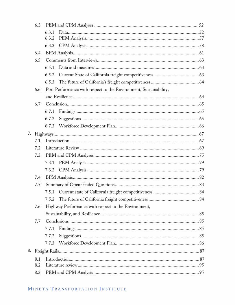
3.3 The PEM and CPM Approaches Lambert and Sharma (1990) first proposed the framework of the Performance Evaluation Matrix (PEM) and the Competitive Position Matrix (CPM) for competitive analysis, as shown in Table 2. They presented a method of collecting and using customer-based competitive data for prioritizing investments for the improvement of customer services. They propose four sequential steps below.
Table 2. Steps for PEM and CPM
Step 1: Identify all customer service attributes used by buyers in the selection and evaluation of vendors;
Step 2: Collect information on the importance of the attributes identified in Step 1 and evaluate the performance of the company and its competitors based on the attributes;
Step 3: Evaluate competitive position and performance through PEM and CPM, respectively;
Step 4: Develop strategies to create a competitive advantage.
The PEM uses a three-by-three matrix with the importance of each measure and the performance ratings, dividing into nine cells, as shown in Figure 1.
Figure 1. Performance Evaluation Matrix (PEM)
M I N E T A T R A N S P O R T A T I O N I N S T I T U T E 7
Competitive Disadvantage Parity
7 5 6 7
9 Measure Major Weakness 2
Improve performance 10 4
5 3 Q) (.) C
8
~ 0 a.
Examine Improve performance
.s 3
Do not Minor Weakness measure
-3 -1 +1
Relative performance
Source: Adopted by Lambert and Shanna ( 1990)
Competitive Advantage
Major Strength Maintain performance High
Medium Maintain performance
Minor Strength Low
+3
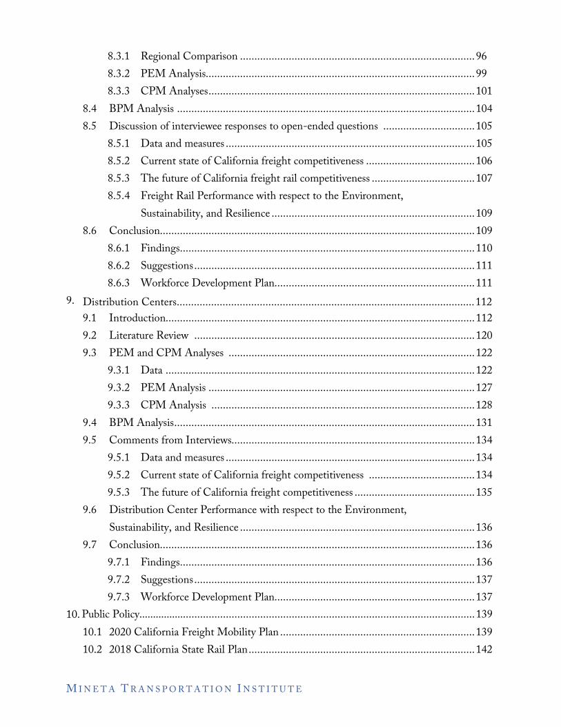
The CPM, shown in Figure 2, has two dimensions: importance and relative performance. The relative performance is the difference between the performance of the focal company and that of the major competitor.
Figure 2. Competitive Position Matrix (CPM)
The nine cells in the matrix are grouped into three broad categories:
• Competitive advantage • Major strength (high importance, high relative performance) • Minor strength (low importance, high relative performance) • Competitive parity • Competitive disadvantage • Major weakness (high importance, low relative performance) • Minor weakness (low importance, low relative performance).
In this study, the PEM provides a self-evaluation of California’s freight performances. California policymakers should maintain the attributes with high importance and higher performance, while improving those with high importance and medium to low performance. The CPM demonstrates the competitive position of California as compared with other states on each performance measure. California policymakers should maintain the measures considered competitive advantages and prioritize improvements based on their importance.
M I N E T A T R A N S P O R T A T I O N I N S T I T U T E 8
This study contributes to the literature by adding two revisions to the frameworks of the CPM and PEM. First, we propose using a percentile scale to measure performance among competing counterparts. Therefore, the performance measures of different units can be compared in the CPM diagram. Additionally, this study proposes using the product of the importance ratings and the average performance percentiles of each attribute from the PEM to compose an overall weighted score for each entity to be compared, such as ports, cities, or states. Furthermore, even though the CPM and PEM can indicate the opportunities for the enhancement of performances and competitiveness, these performance measures from a systematic perspective are not independent but rather are interconnected. Some performance measures are leading indicators of other performance measures. For example, Su and Ke (2017) consider the efficiency of customs clearance and infrastructure as “leading indicators,” which are the key contributors to a country’s competitiveness for international logistics services. They argue that a government should prioritize investments that contribute to the performance of leading indicators. As a result, the performance of the other “lagging indicators” such as timeliness, international shipments, and tracking and tracing will be improved. Hence, in this study, referring to the LPI issued by the World Bank, proposes an enhanced model of CPM and PEM by demonstrating the competitive position of a state and its competitors, from different sectors of freight competitiveness.
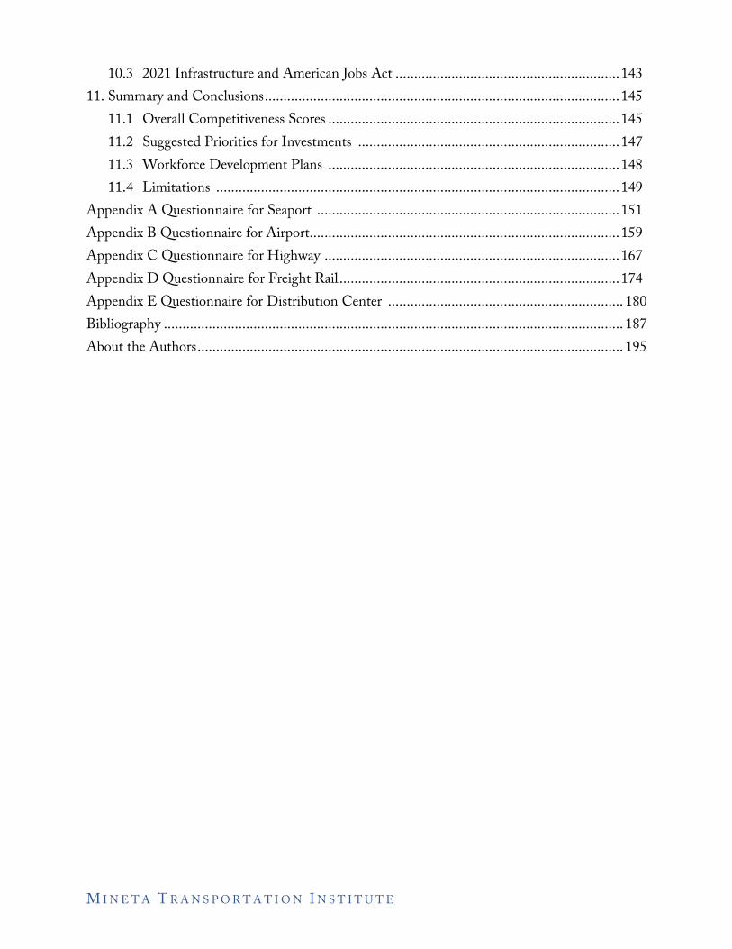
3.4 The BPM Approach The bottleneck of a state’s freight system determines its effectiveness. This project uses the Business Process Management (BPM) approach, proposed by Su and Ke (2017), to identify California’s freight system bottlenecks. Su and Ke (2017) propose an eight-step approach to identify the bottlenecks of a country’s logistics performance, by comparing the focal country’s national logistics performance metrics data against the chosen benchmarked countries. The eight steps are revised for this study as follows (see Figure 3). In this study, we use the overall weighted score and ranking mentioned in Step 1 to compare California with neighboring states, such as Arizona and Washington, and competing states, such as Texas and Georgia, in Step 2 and then conduct Steps 3–8.
M I N E T A T R A N S P O R T A T I O N I N S T I T U T E 9
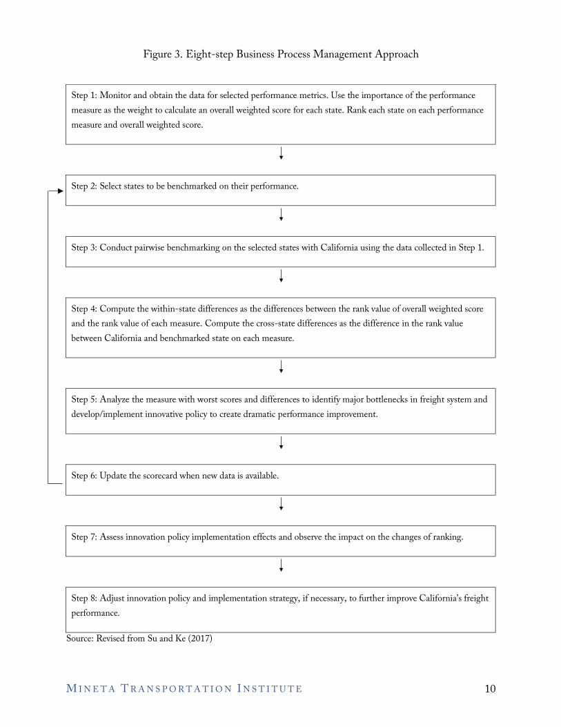
Figure 3. Eight-step Business Process Management Approach
Step 1: Monitor and obtain the data for selected performance metrics. Use the importance of the performance measure as the weight to calculate an overall weighted score for each state. Rank each state on each performance measure and overall weighted score.
Step 2: Select states to be benchmarked on their performance.
Step 3: Conduct pairwise benchmarking on the selected states with California using the data collected in Step 1.
Step 4: Compute the within-state differences as the differences between the rank value of overall weighted score and the rank value of each measure. Compute the cross-state differences as the difference in the rank value between California and benchmarked state on each measure.
Step 5: Analyze the measure with worst scores and differences to identify major bottlenecks in freight system and develop/implement innovative policy to create dramatic performance improvement.
Step 6: Update the scorecard when new data is available.
Step 7: Assess innovation policy implementation effects and observe the impact on the changes of ranking.
Step 8: Adjust innovation policy and implementation strategy, if necessary, to further improve California’s freight performance.
Source: Revised from Su and Ke (2017)
M I N E T A T R A N S P O R T A T I O N I N S T I T U T E 10
4. Competitiveness of the Freight System from the SCM’s Perspective
Competition is not unfolding between individual ports, customs, highways, freight rail, or distribution systems, but between the integrated supply chains of states (De Martino and Morvillo 2008). Transport demand is, after all, a derived demand. Port authorities, railroad operators, road operators, stevedores, shipping lines, depot operations, customs agents, and numerous others exist only based on trade demand (Robinson 2002). Shippers will choose between chains based on competitive advantage and value gained (Robinson 2002). The freight sectors, including ports, highways, freight rail, and distribution centers, must be embedded in supply chains that offer shippers more significant value (Robinson 2002). In this study, we rely on industry experts to evaluate the contributions of each sector to the success of the supply chain in California, using the performance attributes of the Supply Chain Operations Reference (SCOR) Model. The APICS Supply Chain Council (currently known as the Association for Supply Chain Management or ASCM) developed the SCOR Model for supply chain management (SCM) diagnostic benchmarking and process improvements. Practitioners use the SCOR model for benchmarking, to set reasonable performance goals, calculate performance gaps against a global database, and develop company-specific roadmaps for supply chain competitive success. Table 3 reports the performance attributes of the SCOR model.
M I N E T A T R A N S P O R T A T I O N I N S T I T U T E 11
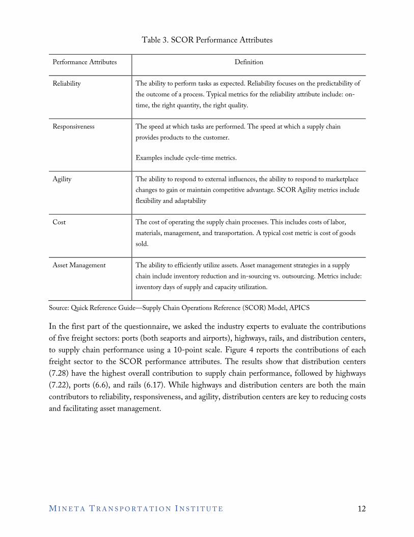
Table 3. SCOR Performance Attributes
Performance Attributes Definition
Reliability The ability to perform tasks as expected. Reliability focuses on the predictability of the outcome of a process. Typical metrics for the reliability attribute include: on-time, the right quantity, the right quality.
Responsiveness The speed at which tasks are performed. The speed at which a supply chain provides products to the customer.
Examples include cycle-time metrics.
Agility The ability to respond to external influences, the ability to respond to marketplace changes to gain or maintain competitive advantage. SCOR Agility metrics include flexibility and adaptability
Cost The cost of operating the supply chain processes. This includes costs of labor, materials, management, and transportation. A typical cost metric is cost of goods sold.
Asset Management The ability to efficiently utilize assets. Asset management strategies in a supply chain include inventory reduction and in-sourcing vs. outsourcing. Metrics include: inventory days of supply and capacity utilization.
Source: Quick Reference Guide—Supply Chain Operations Reference (SCOR) Model, APICS
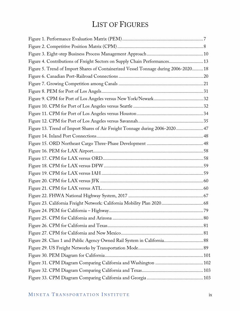
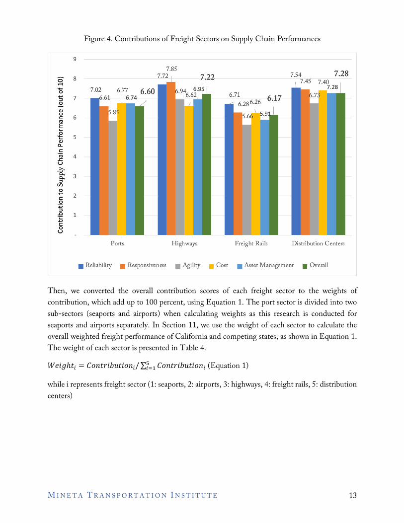
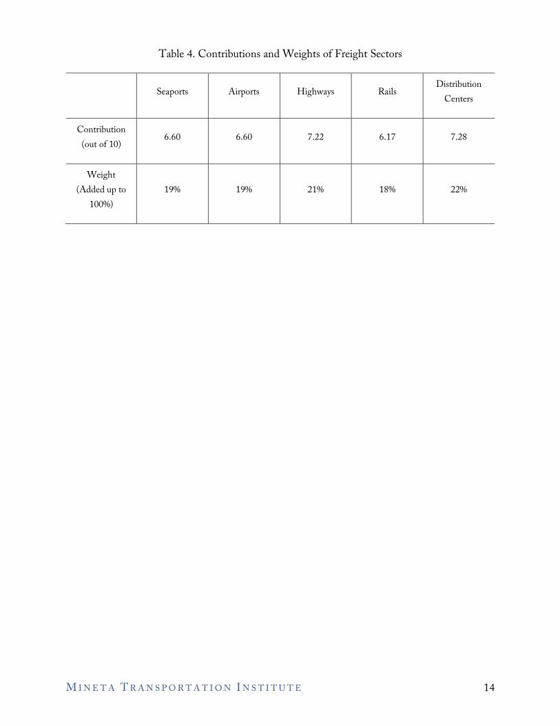
In the first part of the questionnaire, we asked the industry experts to evaluate the contributions of five freight sectors: ports (both seaports and airports), highways, rails, and distribution centers, to supply chain performance using a 10-point scale. Figure 4 reports the contributions of each freight sector to the SCOR performance attributes. The results show that distribution centers (7.28) have the highest overall contribution to supply chain performance, followed by highways (7.22), ports (6.6), and rails (6.17). While highways and distribution centers are both the main contributors to reliability, responsiveness, and agility, distribution centers are key to reducing costs and facilitating asset management.
M I N E T A T R A N S P O R T A T I O N I N S T I T U T E 12
M I N E T A T R A N S P O R T A T I O N I N S T I T U T E 13
Figure 4. Contributions of Freight Sectors on Supply Chain Performances
Then, we converted the overall contribution scores of each freight sector to the weights of contribution, which add up to 100 percent, using Equation 1. The port sector is divided into two sub-sectors (seaports and airports) when calculating weights as this research is conducted for seaports and airports separately. In Section 11, we use the weight of each sector to calculate the overall weighted freight performance of California and competing states, as shown in Equation 1. The weight of each sector is presented in Table 4.
!"#$ℎ&' = )*+&,#-.&#*+'/∑ )*+&,#-.&#*+'1'23 (Equation 1)
while i represents freight sector (1: seaports, 2: airports, 3: highways, 4: freight rails, 5: distribution centers)
M I N E T A T R A N S P O R T A T I O N I N S T I T U T E 14
Table 4. Contributions and Weights of Freight Sectors
Seaports Airports Highways Rails Distribution Centers
Contribution (out of 10) 6.60 6.60 7.22 6.17 7.28
Weight (Added up to
100%) 19% 19% 21% 18% 22%
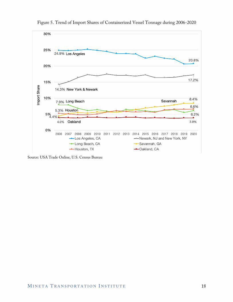
5. Seaports 5.1 Introduction About 60% of the U.S. imports, measured by containerized vessel tonnage, in 2020 were concentrated in five ports: Los Angeles (L.A.) and Long Beach (L.B.), New York and New Jersey, Savannah, and Houston (see Table 5). Navigation time plays a vital role in the port-of-entry decision. The ports in California, including LA, LB, and Oakland, account for 45% of imports from Asia, while the ports on the East Coast like Newark, New York, and Savannah handle 37% of the imports from Europe. However, the import shares of the ports on the East and West Coasts show different trends over the past 20 years, mainly due to the expansion of the Panama Canal, improvement in intermodal and seaport infrastructures, and the U.S.–China trade war. Table 6 and Figure 5 show the trend of the import share of containerized vessel tonnage for the major U.S. ports during 2006–2020. Table 7 reports the year-over-year growth rate and the compounded annual growth rate (CAGR). During 2006–2020, the shares of L.A. and L.B. show a downward trend, and the shares dropped 4.1 % points and 1.7% points, respectively. In contrast, the shares of New York and Newark, and Savannah increased by 2.9% points and 4% points, respectively.
M I N E T A T R A N S P O R T A T I O N I N S T I T U T E 15
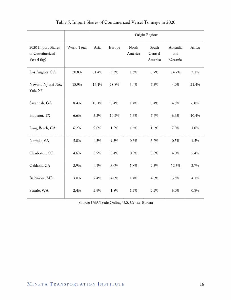
Table 5. Import Shares of Containerized Vessel Tonnage in 2020
Origin Regions
2020 Import Shares World Total Asia Europe North South Australia Africa of Containerized America Central and Vessel (kg) America Oceania
Los Angeles, CA 20.8% 31.4% 5.3% 1.6% 3.7% 14.7% 3.1%
Newark, NJ and New Yok, NY
15.9% 14.1% 28.8% 3.4% 7.5% 4.0% 21.4%
Savannah, GA 8.4% 10.1% 8.4% 1.4% 3.4% 4.5% 6.0%
Houston, TX 6.6% 5.2% 10.2% 5.3% 7.6% 6.6% 10.4%
Long Beach, CA 6.2% 9.0% 1.8% 1.6% 1.6% 7.8% 1.0%
Norfolk, VA 5.0% 4.3% 9.3% 0.3% 3.2% 0.5% 4.5%
Charleston, SC 4.6% 3.9% 8.4% 0.9% 3.0% 4.0% 5.4%
Oakland, CA 3.9% 4.4% 3.0% 1.8% 2.5% 12.5% 2.7%
Baltimore, MD 3.0% 2.4% 4.0% 1.4% 4.0% 3.5% 4.1%
Seattle, WA 2.4% 2.6% 1.8% 1.7% 2.2% 6.0% 0.8%
Source: USA Trade Online, U.S. Census Bureau
M I N E T A T R A N S P O R T A T I O N I N S T I T U T E 16
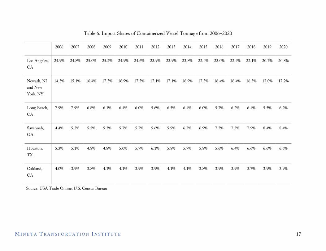
Table 6. Import Shares of Containerized Vessel Tonnage from 2006–2020
2006 2007 2008 2009 2010 2011 2012 2013 2014 2015 2016 2017 2018 2019 2020
Los Angeles, CA
24.9% 24.8% 25.0% 25.2% 24.9% 24.6% 23.9% 23.9% 23.8% 22.4% 23.0% 22.4% 22.1% 20.7% 20.8%
Newark, NJ 14.3% 15.1% 16.4% 17.3% 16.9% 17.5% 17.1% 17.1% 16.9% 17.3% 16.4% 16.4% 16.5% 17.0% 17.2% and New York, NY
Long Beach, CA
7.9% 7.9% 6.8% 6.1% 6.4% 6.0% 5.6% 6.5% 6.4% 6.0% 5.7% 6.2% 6.4% 5.5% 6.2%
Savannah, GA
4.4% 5.2% 5.5% 5.3% 5.7% 5.7% 5.6% 5.9% 6.5% 6.9% 7.3% 7.5% 7.9% 8.4% 8.4%
Houston, TX
5.3% 5.1% 4.8% 4.8% 5.0% 5.7% 6.1% 5.8% 5.7% 5.8% 5.6% 6.4% 6.6% 6.6% 6.6%
Oakland, CA
4.0% 3.9% 3.8% 4.1% 4.1% 3.9% 3.9% 4.1% 4.1% 3.8% 3.9% 3.9% 3.7% 3.9% 3.9%
Source: USA Trade Online, U.S. Census Bureau
M I N E T A T R A N S P O R T A T I O N I N S T I T U T E 17
<ti .c Cl)
30%
25%
20%
15%
24.9% Los Angeles
20.8%
17.2%
14.3% New York & Newark
t:: c.o 10% 8 4o/c
7.9% Long Beach Savannah • 0
£ 5% s~;?i? .... ::--;:::;,--- :: <1-e'. ; :..-: :~: 4.4% ~--------___,.__ ___ _._ __________ ..._ _______ __. ___ __,
4.0% Oakland 3.9%
0% 2006 2007 2008 2009 2010 2011 2012 2013 2014 2015 2016 2017 2018 2019 2020
--Los Angeles, CA --Newark, NJ and New York, NY
--Long Beach, CA --savannah, GA
--Houston, TX --Oakland, CA
Figure 5. Trend of Import Shares of Containerized Vessel Tonnage during 2006-2020
Source: USA Trade Online, U.S. Census Bureau
M I N E T A T R A N S P O R T A T I O N I N S T I T U T E 18
Table 7. Growth of Containerized Vessel Tonnage from 2006–2020
2006 2007 2008 2009 2010 2011 2012 2013 2014 2015 2016 2017 2018 2019 2020 CAGR
Los Angeles, 15.8% -1.2% -5.2% -17.3% 13.7% 4.1% 2.2% -0.2% 6.5% 0.7% 2.2% 1.9% 3.4% -8.0% 2.0% 0.1% CA
Newark, NJ 0.2% 5.1% 2.3% -13.8% 12.7% 9.2% 2.4% 0.0% 5.4% 9.2% -5.5% 4.8% 5.3% 1.3% 3.1% 2.8% and New York, NY
Long Beach, 18.0% -1.3% -18.7% -26.6% 20.8% -2.3% -0.9% 14.8% 6.1% 0.6% -5.4% 13.8% 7.6% -14.8% 12.8% -0.4% CA
Savannah, GA 0.4% 16.5% -0.7% -20.3% 22.9% 4.7% 4.2% 5.7% 16.6% 14.6% 4.7% 7.6% 10.5% 4.8% 1.5% 6.2%
Houston, TX 3.2% -5.0% -10.3% -18.4% 20.3% 19.6% 12.8% -5.4% 5.6% 8.2% -4.3% 19.5% 7.9% -1.3% 2.5% 3.0%
Oakland, CA 10.9% -2.3% -8.0% -12.5% 14.3% 1.3% 5.5% 3.8% 7.4% -0.1% 2.3% 3.0% 1.2% 1.8% 1.5% 1.2%
U.S. Total 5.5% -0.9% -5.8% -18.1% 15.2% 5.6% 4.9% -0.2% 7.2% 6.6% -0.5% 4.6% 4.8% -1.4% 1.4% 1.4%
Source: USA Trade Online, U.S. Census Bureau
M I N E T A T R A N S P O R T A T I O N I N S T I T U T E 19
I I
+
CN line
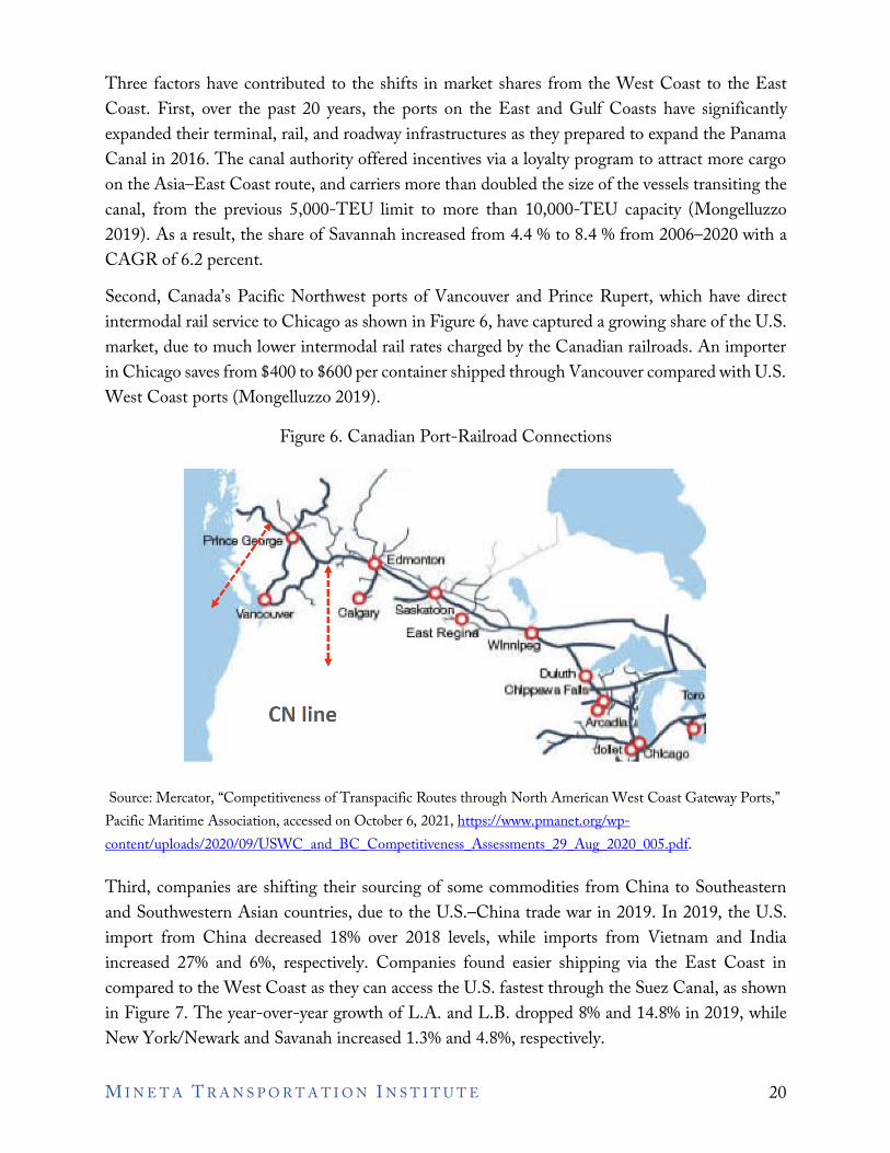
Three factors have contributed to the shifts in market shares from the West Coast to the East Coast. First, over the past 20 years, the ports on the East and Gulf Coasts have significantly expanded their terminal, rail, and roadway infrastructures as they prepared to expand the Panama Canal in 2016. The canal authority offered incentives via a loyalty program to attract more cargo on the Asia–East Coast route, and carriers more than doubled the size of the vessels transiting the canal, from the previous 5,000-TEU limit to more than 10,000-TEU capacity (Mongelluzzo 2019). As a result, the share of Savannah increased from 4.4 % to 8.4 % from 2006–2020 with a CAGR of 6.2 percent. Second, Canada’s Pacific Northwest ports of Vancouver and Prince Rupert, which have direct intermodal rail service to Chicago as shown in Figure 6, have captured a growing share of the U.S. market, due to much lower intermodal rail rates charged by the Canadian railroads. An importer in Chicago saves from $400 to $600 per container shipped through Vancouver compared with U.S. West Coast ports (Mongelluzzo 2019).
Figure 6. Canadian Port-Railroad Connections
Source: Mercator, “Competitiveness of Transpacific Routes through North American West Coast Gateway Ports,” Pacific Maritime Association, accessed on October 6, 2021, https://www.pmanet.org/wp-content/uploads/2020/09/USWC_and_BC_Competitiveness_Assessments_29_Aug_2020_005.pdf.
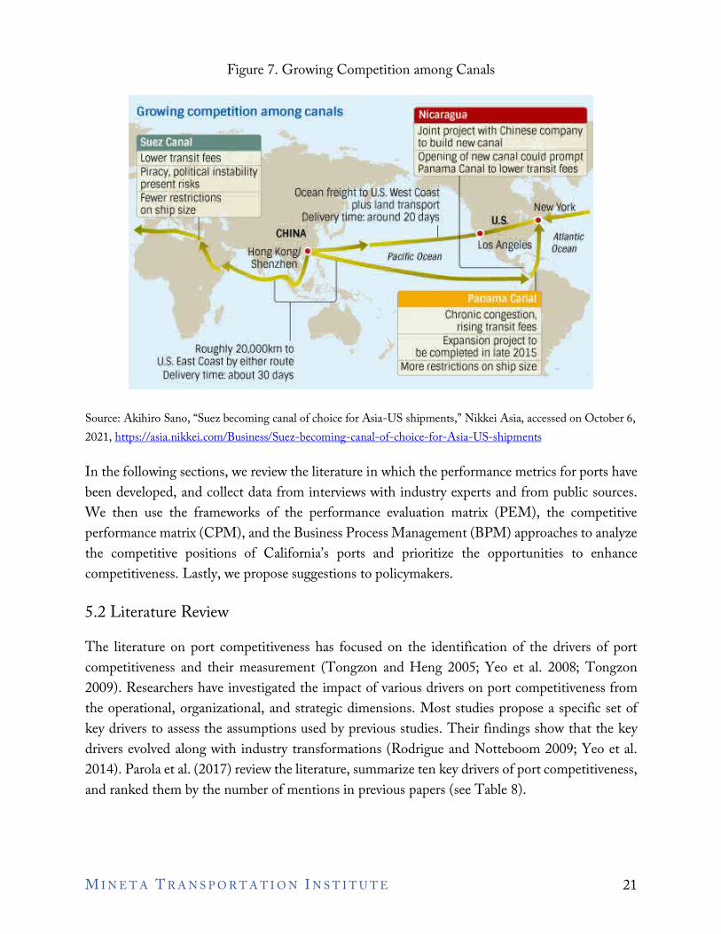
Third, companies are shifting their sourcing of some commodities from China to Southeastern and Southwestern Asian countries, due to the U.S.–China trade war in 2019. In 2019, the U.S. import from China decreased 18% over 2018 levels, while imports from Vietnam and India increased 27% and 6%, respectively. Companies found easier shipping via the East Coast in compared to the West Coast as they can access the U.S. fastest through the Suez Canal, as shown in Figure 7. The year-over-year growth of L.A. and L.B. dropped 8% and 14.8% in 2019, while New York/Newark and Savanah increased 1.3% and 4.8%, respectively.
M I N E T A T R A N S P O R T A T I O N I N S T I T U T E 20
competition among canals
,S~_ Lower transit fees
Nicaragua Joint project with Chinese company to builcl new canal Opening of new canal coulcl prompt Panama canal to lower transit fees Piracy, political instability
present risks Fewer restrictions on ship size
Ocean freight to U.S. West Coast plus lane! transport
Delivery time: around 20 days New York •
CHINA
Hong Kong/• Shenzhen
Roughly 20,000km to U.S. East Coast by either route Delivery time: about 30 clays
Pacific Ocean
Chronic congestion. rising transit fees
Expansion project to be completecl in late 2015
More restrictions on ship size
Atlantic Ocean
Figure 7. Growing Competition among Canals
Source: Akihiro Sano, “Suez becoming canal of choice for Asia-US shipments,” Nikkei Asia, accessed on October 6, 2021, https://asia.nikkei.com/Business/Suez-becoming-canal-of-choice-for-Asia-US-shipments
In the following sections, we review the literature in which the performance metrics for ports have been developed, and collect data from interviews with industry experts and from public sources. We then use the frameworks of the performance evaluation matrix (PEM), the competitive performance matrix (CPM), and the Business Process Management (BPM) approaches to analyze the competitive positions of California’s ports and prioritize the opportunities to enhance competitiveness. Lastly, we propose suggestions to policymakers.
5.2 Literature Review The literature on port competitiveness has focused on the identification of the drivers of port competitiveness and their measurement (Tongzon and Heng 2005; Yeo et al. 2008; Tongzon 2009). Researchers have investigated the impact of various drivers on port competitiveness from the operational, organizational, and strategic dimensions. Most studies propose a specific set of key drivers to assess the assumptions used by previous studies. Their findings show that the key drivers evolved along with industry transformations (Rodrigue and Notteboom 2009; Yeo et al. 2014). Parola et al. (2017) review the literature, summarize ten key drivers of port competitiveness, and ranked them by the number of mentions in previous papers (see Table 8).
M I N E T A T R A N S P O R T A T I O N I N S T I T U T E 21
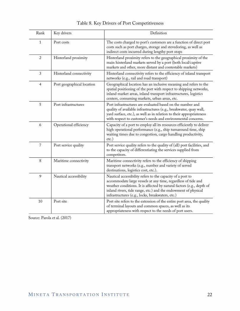
Table 8. Key Drivers of Port Competitiveness Rank Key drivers Definition
1 Port costs The costs charged to port’s customers are a function of direct port costs such as port charges, storage and stevedoring, as well as indirect costs incurred during lengthy port stops
2 Hinterland proximity Hinterland proximity refers to the geographical proximity of the main hinterland markets served by a port (both local/captive markets and other, more distant and contestable markets)
3 Hinterland connectivity Hinterland connectivity refers to the efficiency of inland transport networks (e.g., rail and road transport)
4 Port geographical location Geographical location has an inclusive meaning and refers to the spatial positioning of the port with respect to shipping networks, inland market areas, inland transport infrastructures, logistics centers, consuming markets, urban areas, etc.
5 Port infrastructures Port infrastructures are evaluated based on the number and quality of available infrastructures (e.g., breakwater, quay wall, yard surface, etc.), as well as in relation to their appropriateness with respect to customer’s needs and environmental concerns.
6 Operational efficiency Capacity of a port to employ all its resources efficiently to deliver high operational performance (e.g., ship turnaround time, ship waiting times due to congestion, cargo handling productivity, etc.)
7 Port service quality Port service quality refers to the quality of (all) port facilities, and to the capacity of differentiating the services supplied from competitors.
8 Maritime connectivity Maritime connectivity refers to the efficiency of shipping transport networks (e.g., number and variety of served destinations, logistics cost, etc.).
9 Nautical accessibility Nautical accessibility refers to the capacity of a port to accommodate large vessels at any time, regardless of tide and weather conditions. It is affected by natural factors (e.g., depth of inland rivers, tide range, etc.) and the endowment of physical infrastructures (e.g., locks, breakwaters, etc.)
10 Port site Port site refers to the extension of the entire port area, the quality of terminal layouts and common spaces, as well as its appropriateness with respect to the needs of port users.
Source: Parola et al. (2017)
M I N E T A T R A N S P O R T A T I O N I N S T I T U T E 22
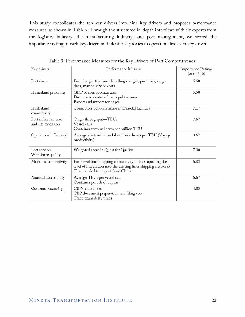
This study consolidates the ten key drivers into nine key drivers and proposes performance measures, as shown in Table 9. Through the structured in-depth interviews with six experts from the logistics industry, the manufacturing industry, and port management, we scored the importance rating of each key driver, and identified proxies to operationalize each key driver.
Table 9. Performance Measures for the Key Drivers of Port Competitiveness Key drivers Performance Measure Importance Ratings
(out of 10) Port costs Port charges (terminal handling charges, port dues, cargo
dues, marine service cost) 5.50
Hinterland proximity GDP of metropolitan area Distance to center of metropolitan area Export and import tonnages
5.50
Hinterland connectivity
Connectors between major intermodal facilities 7.17
Port infrastructures and site extension
Cargo throughput—TEUs Vessel calls Container terminal acres per million TEU
7.67
Operational efficiency Average container vessel dwell time hours per TEU (Voyage productivity)
8.67
Port service/ Workforce quality
Weighted score in Quest for Quality 7.00
Maritime connectivity Port-level liner shipping connectivity index (capturing the level of integration into the existing liner shipping network) Time needed to import from China
6.83
Nautical accessibility Average TEUs per vessel call Container port draft depths
6.67
Customs processing CBP-related fees CBP document preparation and filing costs Trade exam delay times
4.83
M I N E T A T R A N S P O R T A T I O N I N S T I T U T E 23
The public sources for port statistics are summarized as follows:
• The U.S. Bureau of Transportation Statistics provides the port performance freight statistics, including cargo throughput (tonnage and TEU), vessel calls, container vessel dwell time, container port draft depths, and the container terminal acres.
• MARAD (the Maritime Administration, the U.S. Department of Transportation) produces an annual statistical snapshot that provides nearly 20 categories of water-freight related statistics. The statistics address freight volumes, ports of entry and export, commodity trends, numbers of ships and containers involved, and trade measures.
• The U.S. Census Bureau provides monthly data about the trade volume and containerized vessel tonnage of U.S. ports through the U.S.A. Trade Online website.
• The U.S. Bureau of Economic Analysis provides the real GDP for the top 50 metropolitan statistical areas.
• The distance of a port to the center of the closest metropolitan areas is calculated from Google maps.
• The United Nations Conference on Trade and Development (UNCTAD) publishes the Liner Shipping Connectivity Index (LSCI), which captures how well countries and ports are connected to global shipping networks. The LSCI consists of five components of the maritime transport sector: number of ships, their container-carrying capacity, maximum vessel size, number of services, and companies that deploy container ships in a country's ports.
• The Federal Highway Administration publishes data about intermodal connectors, which are roads that provide access between major intermodal facilities and the other four subsystems making up the National Highway System of each state.
5.3 PEM and CPM Analyses In this section, we employ the Performance Evaluation Matrix (PEM) and Competitive Performance Matrix (CPM) developed by Lambert and Sharma (1990) and analyze the competitive position of California’s ports. First, Section 5.3.1 reports the data used for the port comparison. Second, the PEM approach is used to analyze California’s strengths and weaknesses in section 5.3.2. The PEM consists of the performance percentile of the focal port, and the importance rating for each performance measure. The overall weighted score for a port is calculated as the product of the importance ratings and the performance percentiles. In Section 5.3.3, the CPM analysis reveals California’s competitive value relative to these of competing ports. The CPM consists of the differences in performance percentile between the focal port and compared port and the importance rating for each performance measure.
5.3.1 Data
This section summarizes the data collected from multiple public sources for the performance measures of major U.S. ports, as shown in Table 10.
M I N E T A T R A N S P O R T A T I O N I N S T I T U T E 24
Table 11 reports the overall weighted scores, which are the product of weight ratings and performance percentiles, and Table 12 reports the competitiveness ranking of the top 20 U.S. ports. The top six ports in the U.S. are:
(1) Los Angeles, CA; (2) New York, NY and Newark, NJ; (3) Long Beach, CA; (4) Seattle, WA; (5) Houston, TX; (6) Savanah, GA.
California owns two ports which are ranked top 6 in the U.S. The ports of New York and Newark, Seattle, Houston, and Savanah make up the remaining the top ports and thus can viewed as the direct competitors to the ports in California.
M I N E T A T R A N S P O R T A T I O N I N S T I T U T E 25
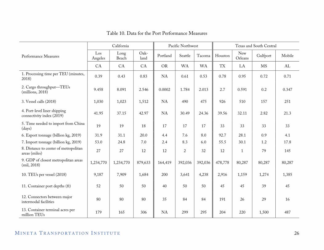
Table 10. Data for the Port Performance Measures
Performance Measures
California Pacific Northwest Texas and South Central Los
Angeles Long Beach
Oak-land Portland Seattle Tacoma Houston New
Orleans Gulfport Mobile
CA CA CA OR WA WA TX LA MS AL 1. Processing time per TEU (minutes, 2018) 0.39 0.43 0.83 NA 0.61 0.53 0.78 0.95 0.72 0.71
2. Cargo throughput—TEUs (millions, 2018) 9.458 8.091 2.546 0.0002 1.784 2.013 2.7 0.591 0.2 0.347
3. Vessel calls (2018) 1,030 1,023 1,512 NA 490 475 926 510 157 251
4. Port-level liner shipping connectivity index (2019) 41.95 37.15 42.97 NA 30.49 24.36 39.56 32.11 2.82 21.3
5. Time needed to import from China (days) 19 19 18 17 17 17 33 33 33 33
6. Export tonnage (billion kg, 2019) 31.9 31.1 20.0 4.4 7.6 8.0 92.7 28.1 0.9 4.1 7. Import tonnage (billion kg, 2019) 53.0 24.8 7.0 2.4 8.3 6.0 55.5 30.1 1.2 17.8 8. Distance to center of metropolitan areas (miles) 27 27 12 12 2 32 12 1 79 145
9. GDP of closest metropolitan areas (mil, 2018) 1,234,770 1,234,770 879,633 164,419 392,036 392,036 478,778 80,287 80,287 80,287
10. TEUs per vessel (2018) 9,187 7,909 1,684 200 3,641 4,238 2,916 1,159 1,274 1,385
11. Container port depths (ft) 52 50 50 40 50 50 45 45 39 45
12. Connectors between major intermodal facilities 80 80 80 35 84 84 191 26 29 16
13. Container terminal acres per million TEUs 179 165 306 NA 299 295 204 220 1,500 487
M I N E T A T R A N S P O R T A T I O N I N S T I T U T E 26
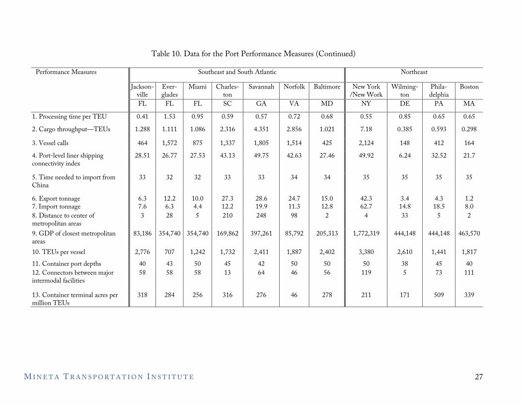
Table 10. Data for the Port Performance Measures (Continued)
Performance Measures Southeast and South Atlantic Northeast
Jackson-ville
Ever-glades
Miami Charles-ton
Savannah Norfolk Baltimore New York /New Work
Wilming-ton
Phila-delphia
Boston
FL FL FL SC GA VA MD NY DE PA MA 1. Processing time per TEU 0.41 1.53 0.95 0.59 0.57 0.72 0.68 0.55 0.85 0.65 0.65 2. Cargo throughput—TEUs 1.288 1.111 1.086 2.316 4.351 2.856 1.021 7.18 0.385 0.593 0.298 3. Vessel calls 464 1,572 875 1,337 1,805 1,514 425 2,124 148 412 164 4. Port-level liner shipping connectivity index
28.51 26.77 27.53 43.13 49.75 42.63 27.46 49.92 6.24 32.52 21.7
5. Time needed to import from China
33 32 32 33 33 34 34 35 35 35 35
6. Export tonnage 6.3 12.2 10.0 27.3 28.6 24.7 15.0 42.3 3.4 4.3 1.2 7. Import tonnage 7.6 6.3 4.4 12.2 19.9 11.3 12.8 62.7 14.8 18.5 8.0 8. Distance to center of metropolitan areas
3 28 5 210 248 98 2 4 33 5 2
9. GDP of closest metropolitan areas
83,186 354,740 354,740 169,862 397,261 85,792 205,313 1,772,319 444,148 444,148 463,570
10. TEUs per vessel 2,776 707 1,242 1,732 2,411 1,887 2,402 3,380 2,610 1,441 1,817 11. Container port depths 40 43 50 45 42 50 50 50 38 45 40 12. Connectors between major intermodal facilities
58 58 58 13 64 46 56 119 5 73 111
13. Container terminal acres per million TEUs
318 284 256 316 276 46 278 211 171 509 339
M I N E T A T R A N S P O R T A T I O N I N S T I T U T E 27
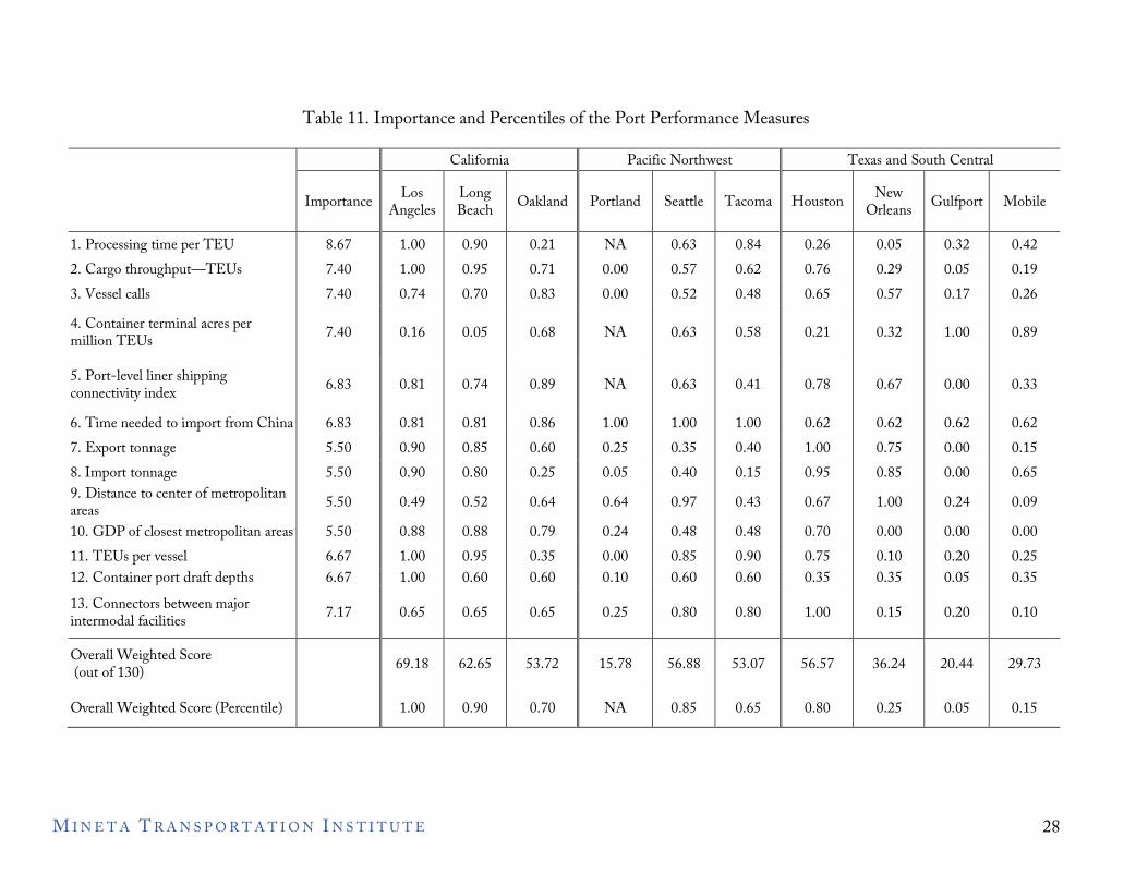
Table 11. Importance and Percentiles of the Port Performance Measures
California Pacific Northwest Texas and South Central
Importance Los Angeles
Long Beach Oakland Portland Seattle Tacoma Houston New
Orleans Gulfport Mobile
1. Processing time per TEU 8.67 1.00 0.90 0.21 NA 0.63 0.84 0.26 0.05 0.32 0.42 2. Cargo throughput—TEUs 7.40 1.00 0.95 0.71 0.00 0.57 0.62 0.76 0.29 0.05 0.19 3. Vessel calls 7.40 0.74 0.70 0.83 0.00 0.52 0.48 0.65 0.57 0.17 0.26 4. Container terminal acres per million TEUs 7.40 0.16 0.05 0.68 NA 0.63 0.58 0.21 0.32 1.00 0.89
5. Port-level liner shipping connectivity index 6.83 0.81 0.74 0.89 NA 0.63 0.41 0.78 0.67 0.00 0.33
6. Time needed to import from China 6.83 0.81 0.81 0.86 1.00 1.00 1.00 0.62 0.62 0.62 0.62 7. Export tonnage 5.50 0.90 0.85 0.60 0.25 0.35 0.40 1.00 0.75 0.00 0.15 8. Import tonnage 5.50 0.90 0.80 0.25 0.05 0.40 0.15 0.95 0.85 0.00 0.65 9. Distance to center of metropolitan 5.50 0.49 0.52 0.64 0.64 0.97 0.43 0.67 1.00 0.24 0.09 areas 10. GDP of closest metropolitan areas 5.50 0.88 0.88 0.79 0.24 0.48 0.48 0.70 0.00 0.00 0.00 11. TEUs per vessel 6.67 1.00 0.95 0.35 0.00 0.85 0.90 0.75 0.10 0.20 0.25 12. Container port draft depths 6.67 1.00 0.60 0.60 0.10 0.60 0.60 0.35 0.35 0.05 0.35 13. Connectors between major intermodal facilities 7.17 0.65 0.65 0.65 0.25 0.80 0.80 1.00 0.15 0.20 0.10
Overall Weighted Score (out of 130)
Overall Weighted Score (Percentile)
69.18
1.00
62.65
0.90
53.72
0.70
15.78
NA
56.88
0.85
53.07
0.65
56.57
0.80
36.24
0.25
20.44
0.05
29.73
0.15
M I N E T A T R A N S P O R T A T I O N I N S T I T U T E 28
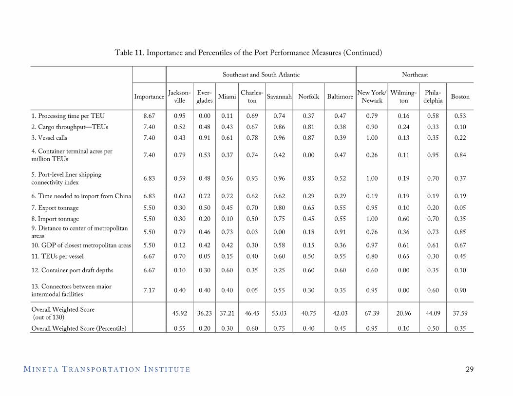
Table 11. Importance and Percentiles of the Port Performance Measures (Continued)
Southeast and South Atlantic Northeast
Importance Jackson-ville
Ever-glades Miami Charles-
ton Savannah Norfolk Baltimore New York/ Newark
Wilming-ton
Phila-delphia Boston
1. Processing time per TEU 8.67 0.95 0.00 0.11 0.69 0.74 0.37 0.47 0.79 0.16 0.58 0.53 2. Cargo throughput—TEUs 7.40 0.52 0.48 0.43 0.67 0.86 0.81 0.38 0.90 0.24 0.33 0.10 3. Vessel calls 7.40 0.43 0.91 0.61 0.78 0.96 0.87 0.39 1.00 0.13 0.35 0.22 4. Container terminal acres per million TEUs 7.40 0.79 0.53 0.37 0.74 0.42 0.00 0.47 0.26 0.11 0.95 0.84
5. Port-level liner shipping connectivity index 6.83 0.59 0.48 0.56 0.93 0.96 0.85 0.52 1.00 0.19 0.70 0.37
6. Time needed to import from China 6.83 0.62 0.72 0.72 0.62 0.62 0.29 0.29 0.19 0.19 0.19 0.19 7. Export tonnage 5.50 0.30 0.50 0.45 0.70 0.80 0.65 0.55 0.95 0.10 0.20 0.05 8. Import tonnage 5.50 0.30 0.20 0.10 0.50 0.75 0.45 0.55 1.00 0.60 0.70 0.35 9. Distance to center of metropolitan 5.50 0.79 0.46 0.73 0.03 0.00 0.18 0.91 0.76 0.36 0.73 0.85 areas 10. GDP of closest metropolitan areas 5.50 0.12 0.42 0.42 0.30 0.58 0.15 0.36 0.97 0.61 0.61 0.67 11. TEUs per vessel 6.67 0.70 0.05 0.15 0.40 0.60 0.50 0.55 0.80 0.65 0.30 0.45 12. Container port draft depths 6.67 0.10 0.30 0.60 0.35 0.25 0.60 0.60 0.60 0.00 0.35 0.10
13. Connectors between major intermodal facilities 7.17 0.40 0.40 0.40 0.05 0.55 0.30 0.35 0.95 0.00 0.60 0.90
Overall Weighted Score (out of 130)
Overall Weighted Score (Percentile)
45.92
0.55
36.23
0.20
37.21
0.30
46.45
0.60
55.03
0.75
40.75
0.40
42.03
0.45
67.39
0.95
20.96
0.10
44.09
0.50
37.59
0.35
M I N E T A T R A N S P O R T A T I O N I N S T I T U T E 29
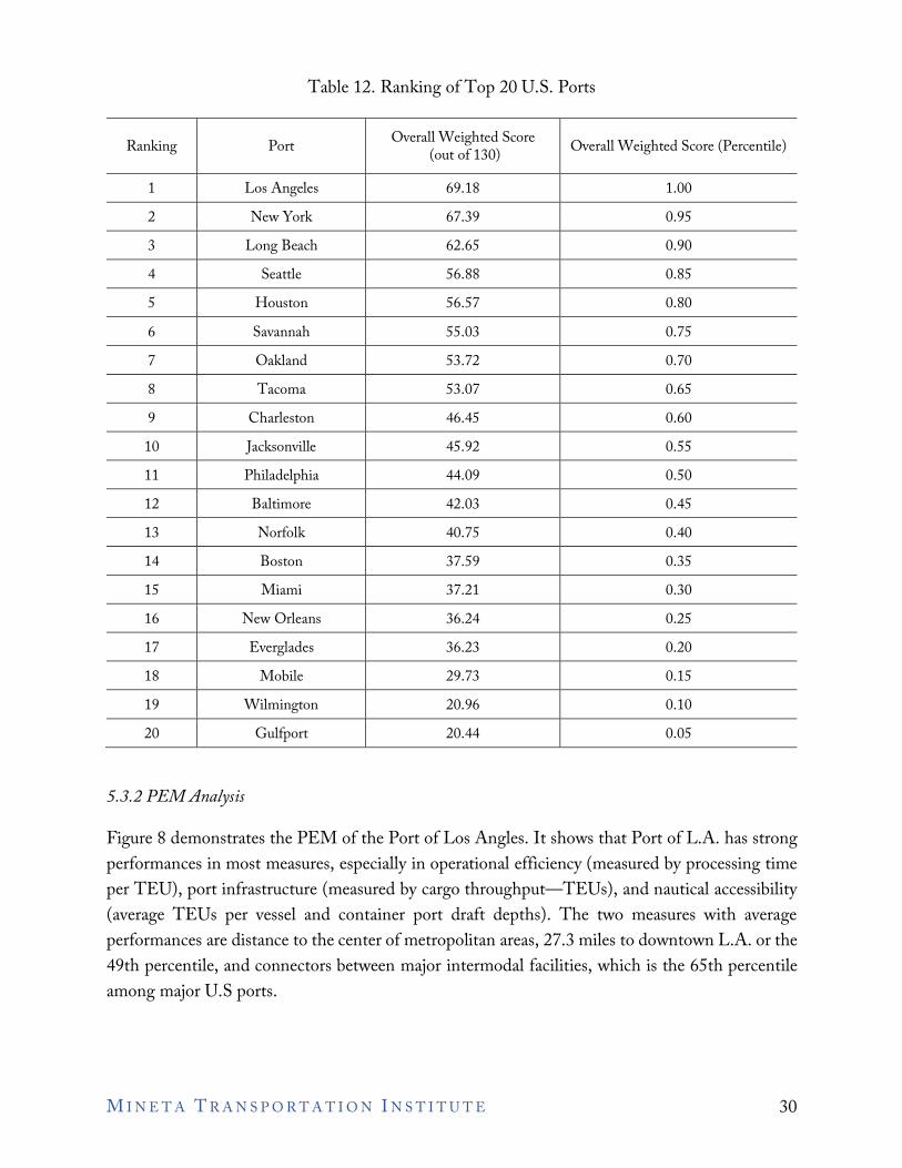
Table 12. Ranking of Top 20 U.S. Ports
Ranking Port Overall Weighted Score (out of 130) Overall Weighted Score (Percentile)
1 Los Angeles 69.18 1.00 2 New York 67.39 0.95 3 Long Beach 62.65 0.90 4 Seattle 56.88 0.85 5 Houston 56.57 0.80 6 Savannah 55.03 0.75 7 Oakland 53.72 0.70 8 Tacoma 53.07 0.65 9 Charleston 46.45 0.60 10 Jacksonville 45.92 0.55 11 Philadelphia 44.09 0.50 12 Baltimore 42.03 0.45 13 Norfolk 40.75 0.40 14 Boston 37.59 0.35 15 Miami 37.21 0.30 16 New Orleans 36.24 0.25 17 Everglades 36.23 0.20 18 Mobile 29.73 0.15 19 Wilmington 20.96 0.10 20 Gulfport 20.44 0.05
5.3.2 PEM Analysis
Figure 8 demonstrates the PEM of the Port of Los Angles. It shows that Port of L.A. has strong performances in most measures, especially in operational efficiency (measured by processing time per TEU), port infrastructure (measured by cargo throughput—TEUs), and nautical accessibility (average TEUs per vessel and container port draft depths). The two measures with average performances are distance to the center of metropolitan areas, 27.3 miles to downtown L.A. or the 49th percentile, and connectors between major intermodal facilities, which is the 65th percentile among major U.S ports.
M I N E T A T R A N S P O R T A T I O N I N S T I T U T E 30
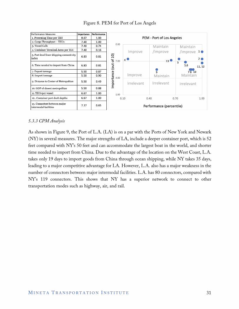
Measures Importance Performance
1. Processing Time per TEU 8.67 1.00 PEM - Port of Los Angeles 2. Cargo Throughput - TEUs 7.40 1.00 3. Vessel Calls 7.40 0.74
0.00 Maintain Maintain
4. Container Terminal Acres per TEU 7.40 0.16
5. Port-level liner shipping connectivity 6.83 0.81
index
6. Time needed to import from China 6.83 0.81
7. Export tonnage 5.50 0.87 8. Import tonnage 5.50 0.90
9. Distance to Center of Metropolitan 5.50 0.49
10. GDP of closest metropolitan 5.50 0.88
Improve /Improve /Improve 1e 0 .-i
4. • 2e 0 7.00 13. ..... 3 • • ::, 5,6 11,12 ~ • -QI 9 78 10 u
Improve Maintain C: Maintain ~ 4.00 .... 0
Irrelevant Irrelevant Irrelevant C. E
11. TEUs per vessel 6.67 1.00 1.00
12 .. Container port draft depths 6.67 1.00 0.10 0.40 0.70 1.00
13. Connectors between major 7.17 0.65
intermodal facilities Performance (percentile)
Figure 8. PEM for Port of Los Angels
5.3.3 CPM Analysis
As shown in Figure 9, the Port of L.A. (LA) is on a par with the Ports of New York and Newark (NY) in several measures. The major strengths of LA, include a deeper container port, which is 52 feet compared with NY’s 50 feet and can accommodate the largest boat in the world, and shorter time needed to import from China. Due to the advantage of the location on the West Coast, L.A. takes only 19 days to import goods from China through ocean shipping, while NY takes 35 days, leading to a major competitive advantage for LA. However, L.A. also has a major weakness in the number of connectors between major intermodal facilities. L.A. has 80 connectors, compared with NY’s 119 connectors. This shows that NY has a superior network to connect to other transportation modes such as highway, air, and rail.
M I N E T A T R A N S P O R T A T I O N I N S T I T U T E 31
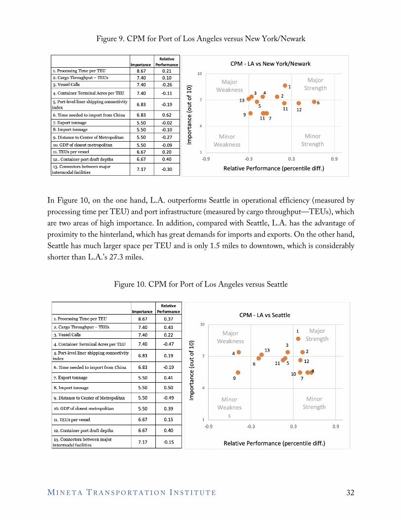
Importance
1. Processing Time per TEU 8.67 2. Cargo Throughput - TEUs 7.40 3. Vessel Calls 7.40
4. Container Terminal Acres per TEU 7.40
5. Port-level liner shipping connectivity 6.83
index
6. Time needed to import from China 6.83
7. Export tonnage 5.50 8. Im port tonnage 5.50
9. Distance to Center of Metropolitan 5.50
10. GDP of closest metropolitan 5.50 11. TEUs per vessel 6.67
12 .. Container port draft depths 6.67
13. Connectors between major 7.17
intermodal facilities
Importance
1. Processing Time per TEU 8.67
2. Cargo Throughput - TEUs 7.40
3. Vessel Calls 7.40
4. Container Terminal Acres per TEU 7.40
5. Port-level liner shipping connectivity 6.83
index
6. Time needed to import from China 6.83
7. Export tonnage 5.50
8. Import tonnage 5.50
9. Distance to Center of Metropolitan 5.50
10. GDP of closest metropolitan 5.50
11. TEUs per vessel 6.67
12. Container port draft depths 6.67
13. Connectors between major 7.17
intermodal facilities
Relative Performance
0.21
0.10 -0.26
-0.11
-0.19
0.62
-0.02
-0.10
-0.27
-0.09
0.20
0.40
-0.30
Relative
Performance
0.37
0.43
0.22
-0.47
0.19
-0.19
0.41
0.50
-0.49
0.39
0.15
0.40
-0.15
0 ...... -0 .., ::,
2. (U u C
10
7
!ti 4 t 0 C. E
-0.9
10
0 ...... -0 .., ::,
2. (U u C !ti t 0 4 C. E
-0.9
CPM - LA vs New York/Newark
Major Weakness
3 4
13-.·
Minor Weakness
9.
-0.3
5 -11 7
•1
e2
• 11
0.3
Major Strength
• .6
12
Minor Strength
Relative Performance (percentile diff.)
CPM - LA vs Seattle
Major 1 Major
Weakness • Strength 3
4. 13 • e2 •• 11-5 • 12
6
• 10• 9 7
Minor Minor Weaknes Strength
s
-0.3 0.3
Relative Performance (percentile diff.)
0.9
0.9
Figure 9. CPM for Port of Los Angeles versus New York/Newark
In Figure 10, on the one hand, L.A. outperforms Seattle in operational efficiency (measured by processing time per TEU) and port infrastructure (measured by cargo throughput—TEUs), which are two areas of high importance. In addition, compared with Seattle, L.A. has the advantage of proximity to the hinterland, which has great demands for imports and exports. On the other hand, Seattle has much larger space per TEU and is only 1.5 miles to downtown, which is considerably shorter than L.A.’s 27.3 miles.
Figure 10. CPM for Port of Los Angeles versus Seattle
M I N E T A T R A N S P O R T A T I O N I N S T I T U T E 32
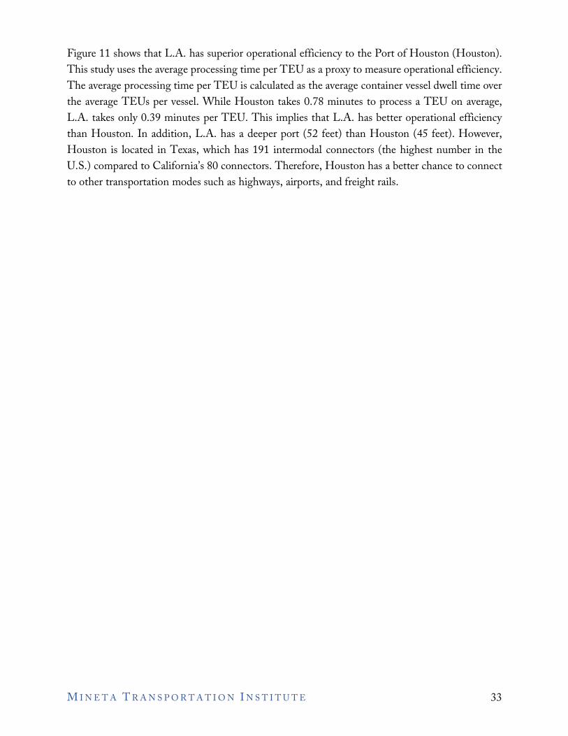
Figure 11 shows that L.A. has superior operational efficiency to the Port of Houston (Houston). This study uses the average processing time per TEU as a proxy to measure operational efficiency. The average processing time per TEU is calculated as the average container vessel dwell time over the average TEUs per vessel. While Houston takes 0.78 minutes to process a TEU on average, L.A. takes only 0.39 minutes per TEU. This implies that L.A. has better operational efficiency than Houston. In addition, L.A. has a deeper port (52 feet) than Houston (45 feet). However, Houston is located in Texas, which has 191 intermodal connectors (the highest number in the U.S.) compared to California’s 80 connectors. Therefore, Houston has a better chance to connect to other transportation modes such as highways, airports, and freight rails.
M I N E T A T R A N S P O R T A T I O N I N S T I T U T E 33
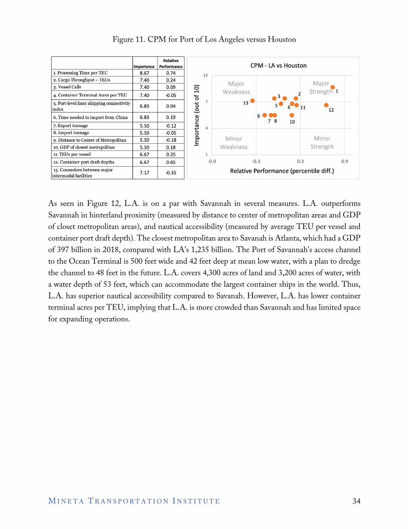
Importance Performance CPM - LA vs Houston 1. Processing Time per TEU 8.67 0.74 10 2. Cargo Throughput - TE Us 7.40 0.24
3. Vessel Calls 7.40 0.09
4. Container Terminal Acres per TEU 7.40 -0.05
5. Port-level liner shipping connectivity 6.83 0.04
index
6. Time needed to import from China 6.83 0.19
7. Export tonnage 5.50 -0.12 8. Import tonnage 5.50 -0.05
9. Distance to Center of Metropolitan 5.50 -0.18
10. GDP of closest metropolitan 5.50 0.18
0 Major Major•
.-t Weakness 2 Strengtti 1 - .3. 0 7 13. • .... s• 6••11 :::, • ~ 12
QI 9·- • u 7 8 10 C: ro 4 .... ... 0 a. Minor Minor E
Weakness Strength 11. TEUs per vessel 6.67 0.25 1
12. Container port draft depths 6.67 0.65 -0.9 -0.3 0.3 0.9
13. Connectors between major 7.17 -0.35 intermodal facilities
Relative Performance (percentile diff.)
Figure 11. CPM for Port of Los Angeles versus Houston
As seen in Figure 12, L.A. is on a par with Savannah in several measures. L.A. outperforms Savannah in hinterland proximity (measured by distance to center of metropolitan areas and GDP of closet metropolitan areas), and nautical accessibility (measured by average TEU per vessel and container port draft depth). The closest metropolitan area to Savanah is Atlanta, which had a GDP of 397 billion in 2018, compared with LA’s 1,235 billion. The Port of Savannah's access channel to the Ocean Terminal is 500 feet wide and 42 feet deep at mean low water, with a plan to dredge the channel to 48 feet in the future. L.A. covers 4,300 acres of land and 3,200 acres of water, with a water depth of 53 feet, which can accommodate the largest container ships in the world. Thus, L.A. has superior nautical accessibility compared to Savanah. However, L.A. has lower container terminal acres per TEU, implying that L.A. is more crowded than Savannah and has limited space for expanding operations.
M I N E T A T R A N S P O R T A T I O N I N S T I T U T E 34
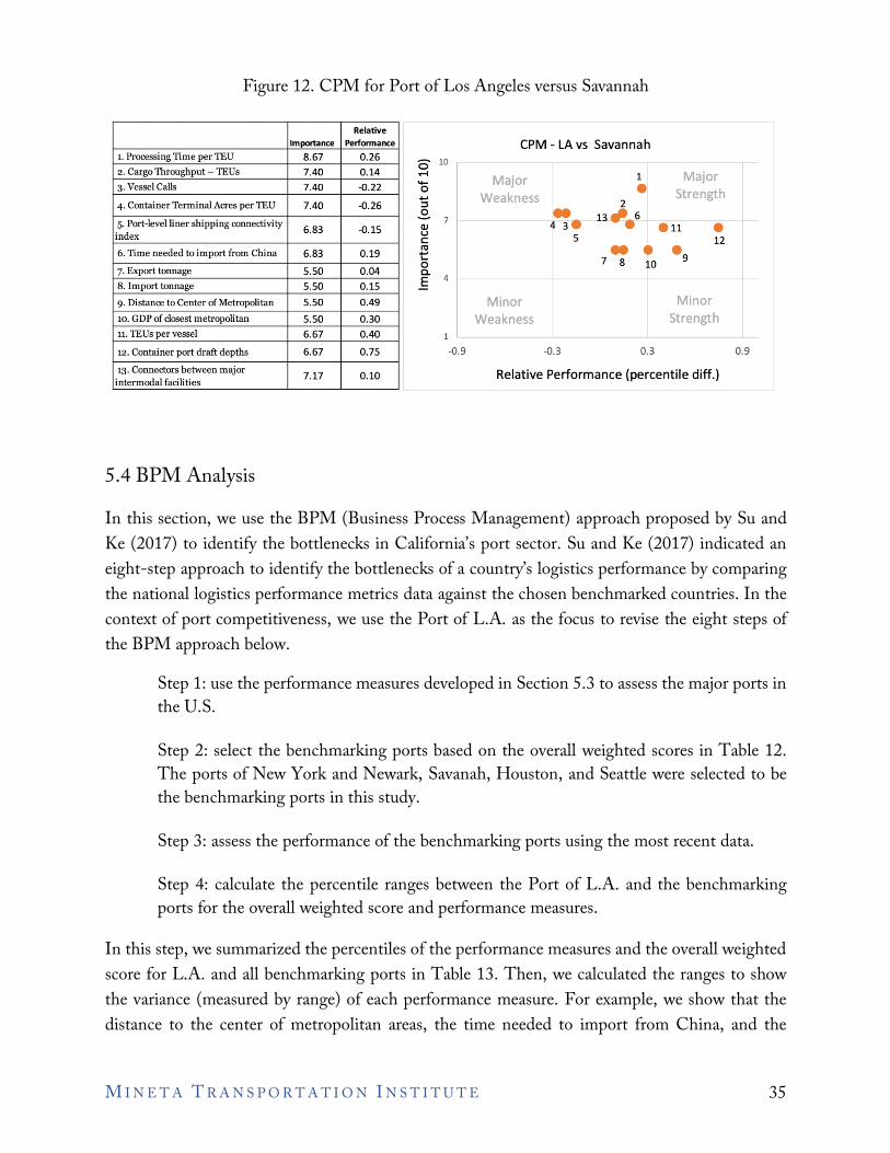
Importance Perfonnance CPM - LA vs Savannah 1. Processing Time per TEU 8.67 0.26 2. Cargo Throughput - TEUs 7.40 0.14 3. Vessel Calls 7.40 -0.22
4. Container Terminal Acres per TEU 7.40 -0.26
5. Port-level liner shipping connectivity 6.83 -0.15
index
0 10 .-4
Major 1 Major -0 • Strength .., Weakness 2 ::,
.£ 7 - 13f/J.6 Qj 4 3. eu • u
5 C 12 6. Time needed to import from China 6.83 0.19
7. Export tonnage 5.50 0.04 8. Import tonnage 5.50 0.15
ro -• .9 t:: 7 8 0 10 a.
4 E
9. Distance to Center of Metropolitan 5.50 0.49 Minor Minor 10. GDP of closest metropolitan 5.50 0.30 Weakness Strength 11. TEUs per vessel 6.67 0.40 1
12. Container port draft depths 6.67 0.75 -0.9 -0.3 0.3 0.9
13. Connectors between major 7.17 0.10
intermodal facilities Relative Performance (percentile diff.)
Figure 12. CPM for Port of Los Angeles versus Savannah
5.4 BPM Analysis In this section, we use the BPM (Business Process Management) approach proposed by Su and Ke (2017) to identify the bottlenecks in California’s port sector. Su and Ke (2017) indicated an eight-step approach to identify the bottlenecks of a country’s logistics performance by comparing the national logistics performance metrics data against the chosen benchmarked countries. In the context of port competitiveness, we use the Port of L.A. as the focus to revise the eight steps of the BPM approach below.
Step 1: use the performance measures developed in Section 5.3 to assess the major ports in the U.S.
Step 2: select the benchmarking ports based on the overall weighted scores in Table 12. The ports of New York and Newark, Savanah, Houston, and Seattle were selected to be the benchmarking ports in this study.
Step 3: assess the performance of the benchmarking ports using the most recent data.
Step 4: calculate the percentile ranges between the Port of L.A. and the benchmarking ports for the overall weighted score and performance measures.
In this step, we summarized the percentiles of the performance measures and the overall weighted score for L.A. and all benchmarking ports in Table 13. Then, we calculated the ranges to show the variance (measured by range) of each performance measure. For example, we show that the distance to the center of metropolitan areas, the time needed to import from China, and the
M I N E T A T R A N S P O R T A T I O N I N S T I T U T E 35
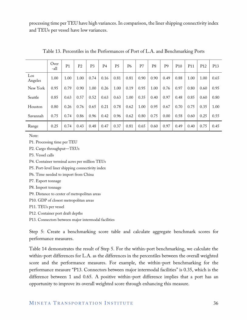
processing time per TEU have high variances. In comparison, the liner shipping connectivity index and TEUs per vessel have low variances.
Table 13. Percentiles in the Performances of Port of L.A. and Benchmarking Ports
Over -all P1 P2 P3 P4 P5 P6 P7 P8 P9 P10 P11 P12 P13
Los Angeles 1.00 1.00 1.00 0.74 0.16 0.81 0.81 0.90 0.90 0.49 0.88 1.00 1.00 0.65
New York 0.95 0.79 0.90 1.00 0.26 1.00 0.19 0.95 1.00 0.76 0.97 0.80 0.60 0.95
Seattle 0.85 0.63 0.57 0.52 0.63 0.63 1.00 0.35 0.40 0.97 0.48 0.85 0.60 0.80
Houston 0.80 0.26 0.76 0.65 0.21 0.78 0.62 1.00 0.95 0.67 0.70 0.75 0.35 1.00
Savannah 0.75 0.74 0.86 0.96 0.42 0.96 0.62 0.80 0.75 0.00 0.58 0.60 0.25 0.55
Range 0.25 0.74 0.43 0.48 0.47 0.37 0.81 0.65 0.60 0.97 0.49 0.40 0.75 0.45
Note: P1. Processing time per TEU P2. Cargo throughput—TEUs P3. Vessel calls P4. Container terminal acres per million TEUs P5. Port-level liner shipping connectivity index P6. Time needed to import from China P7. Export tonnage P8. Import tonnage P9. Distance to center of metropolitan areas P10. GDP of closest metropolitan areas P11. TEUs per vessel P12. Container port draft depths P13. Connectors between major intermodal facilities
Step 5: Create a benchmarking score table and calculate aggregate benchmark scores for performance measures. Table 14 demonstrates the result of Step 5. For the within-port benchmarking, we calculate the within-port differences for L.A. as the differences in the percentiles between the overall weighted score and the performance measures. For example, the within-port benchmarking for the performance measure “P13. Connectors between major intermodal facilities” is 0.35, which is the difference between 1 and 0.65. A positive within-port difference implies that a port has an opportunity to improve its overall weighted score through enhancing this measure.
M I N E T A T R A N S P O R T A T I O N I N S T I T U T E 36
For the cross-port benchmarking, we calculate the cross-port differences for the benchmarking port by comparing the percentiles of performance measures between L.A. and the benchmarking port. For example, the cross-port difference for NY’s “P1. Processing time per TEU” is -0.21, which is the difference between 0.79 (NY) and 1 (LA). It implies that the performance of L.A. is superior to NY’s by 21 percentiles. Thus, a positive cross-port difference indicates an opportunity to improve performances. Lastly, we calculated the aggregate benchmark scores by adding the within-port difference and cross-port differences. For example, the benchmark score of the measure “P1. Processing time per TEU” is -1.58 and is obtained by adding the within-port difference (0) and cross-port differences, including -0.21, -0.37, -0.74, and -0.26. A positive benchmark score1means an opportunity to improve performances, and a higher benchmark score implies a higher priority for the investments to enhance competitiveness.
1 Note that the interpretation on benchmark score in BPM is different from the score on the CPM diagram. While a positive benchmark score in BPM implies an opportunity to improve performances, a negative value in the CPM diagram suggests an opportunity for improvement.
M I N E T A T R A N S P O R T A T I O N I N S T I T U T E 37
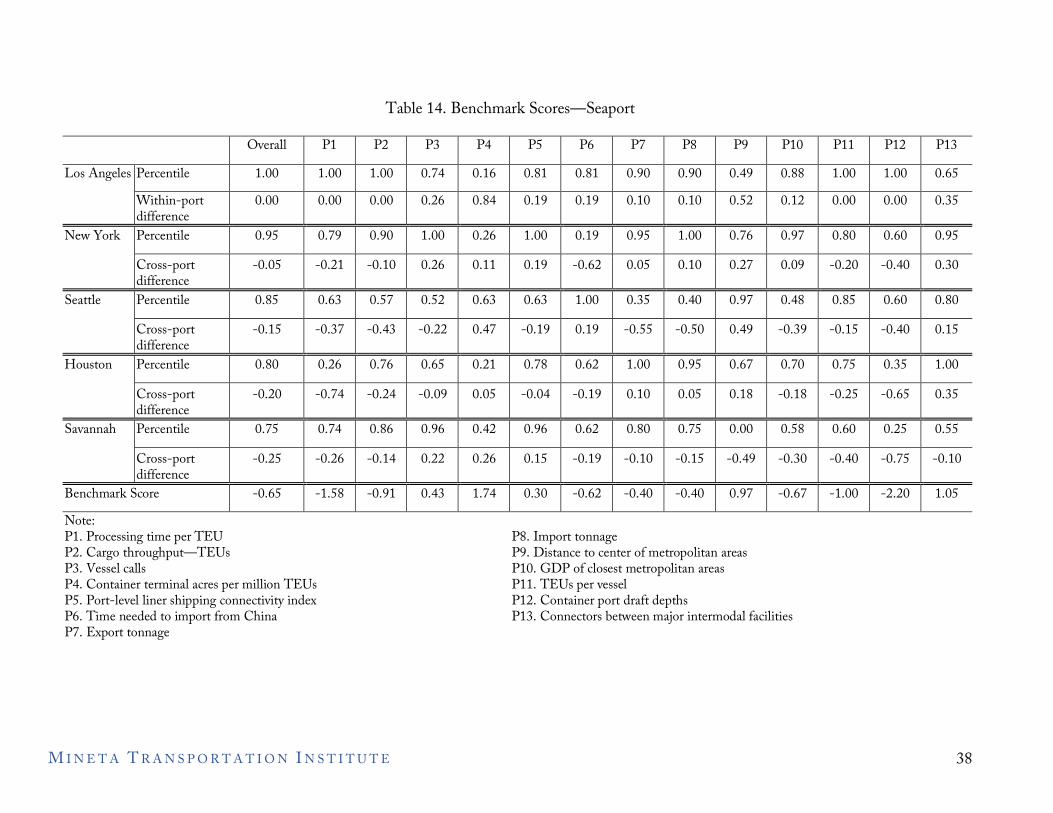
Table 14. Benchmark Scores—Seaport
Overall P1 P2 P3 P4 P5 P6 P7 P8 P9 P10 P11 P12 P13 Los Angeles Percentile 1.00 1.00 1.00 0.74 0.16 0.81 0.81 0.90 0.90 0.49 0.88 1.00 1.00 0.65
Within-port difference
0.00 0.00 0.00 0.26 0.84 0.19 0.19 0.10 0.10 0.52 0.12 0.00 0.00 0.35
New York Percentile 0.95 0.79 0.90 1.00 0.26 1.00 0.19 0.95 1.00 0.76 0.97 0.80 0.60 0.95 Cross-port difference
-0.05 -0.21 -0.10 0.26 0.11 0.19 -0.62 0.05 0.10 0.27 0.09 -0.20 -0.40 0.30
Seattle Percentile 0.85 0.63 0.57 0.52 0.63 0.63 1.00 0.35 0.40 0.97 0.48 0.85 0.60 0.80 Cross-port difference
-0.15 -0.37 -0.43 -0.22 0.47 -0.19 0.19 -0.55 -0.50 0.49 -0.39 -0.15 -0.40 0.15
Houston Percentile 0.80 0.26 0.76 0.65 0.21 0.78 0.62 1.00 0.95 0.67 0.70 0.75 0.35 1.00
Cross-port difference
-0.20 -0.74 -0.24 -0.09 0.05 -0.04 -0.19 0.10 0.05 0.18 -0.18 -0.25 -0.65 0.35
Savannah Percentile 0.75 0.74 0.86 0.96 0.42 0.96 0.62 0.80 0.75 0.00 0.58 0.60 0.25 0.55
Cross-port difference
-0.25 -0.26 -0.14 0.22 0.26 0.15 -0.19 -0.10 -0.15 -0.49 -0.30 -0.40 -0.75 -0.10
Benchmark Score -0.65 -1.58 -0.91 0.43 1.74 0.30 -0.62 -0.40 -0.40 0.97 -0.67 -1.00 -2.20 1.05 Note: P1. Processing time per TEU P2. Cargo throughput—TEUs P3. Vessel calls P4. Container terminal acres per million TEUs P5. Port-level liner shipping connectivity index P6. Time needed to import from China P7. Export tonnage
P8. Import tonnage P9. Distance to center of metropolitan areas P10. GDP of closest metropolitan areas P11. TEUs per vessel P12. Container port draft depths P13. Connectors between major intermodal facilities
M I N E T A T R A N S P O R T A T I O N I N S T I T U T E 38
Step 6: Identify performance measures with higher aggregate benchmark scores as the weak areas of port performance. Based on Table 14, the California government needs to invest in improving the performances of the following measures in order of priority: (1) container terminal acres per million TEUs (1.74); (2) connectors between major intermodal facilities (1.05); (3) distance to center of metropolitan areas (0.97); (4) vessel calls (0.43); and (5) port-level liner shipping connectivity index (0.30). Step 7: Develop policies to improve weak areas of port performance. The suggestions for policymakers to improve port performances are proposed in Section 5.7. Step 8: Track data, percentile, and overall weighted score to check if weak areas are improved.
5.5 Comments from Interviews The above quantitative analysis can be complemented with a qualitative discussion of interviewee responses to open-ended questions. For example, experts were asked about port competitiveness measures, the current and future state of California’s port competitiveness, and related environmental impact, sustainability, and resilience issues.
5.5.1 Data and measures
Experts indicated that the following factors are among the top factors that affect their decision when importers choose a port of entry: costs, speed to market, ability to trans-load merchandise upon arrival, warehouse capacity allowing the ability to redirect, and operational efficiency measured by the speed of turnaround. Importers and exporters might favor a particular location. For example, the ports of L.A. and L.B. are excellent options for importing from east Asia. When selecting a port of entry, all experts indicated that they consider the supply chain as a whole. Performance and reliability are the top factors affecting port selection and are best achieved through major ports and major carriers. Therefore, smaller ports and carriers are struggling. Speed of operation is a key and should have been a measure when evaluating ports, especially related to port efficiency, services, and infrastructure. The average container vessel dwell time is a good measure of the efficiency of loading/unloading, and a better measure should be dwell time per vessel TEU, which is adopted by this study. Intermodal connectivity is an essential factor in the success of a supply chain. Good measures of hinterland connectivity include the number of trans-shipping points, trans-loading points, train connectivity, ability to trans-load merchandise upon arrival, and warehouse capacity that allows for the ability to redirect.
M I N E T A T R A N S P O R T A T I O N I N S T I T U T E 39
M I N E T A T R A N S P O R T A T I O N I N S T I T U T E 40
5.5.2 Current state of California freight competitiveness
Experts believed that the main competition to California’s ocean shipping would be Canada (e.g., Vancouver, Prince Rupert), New York, Newark, Texas (e.g., Houston), and Savannah. They noted that PNW/SeaTac and Vancouver have already drawn away some cargo due to better reliability at ports. The Ports of Vancouver and Prince Rupert have been subsidized by the Canadian government and received huge funds for infrastructure improvements. One expert noted that smaller ports might serve an essential role in stealing away market share as major ports experience bottlenecks. Experts indicated that several investments had been made recently to the infrastructure of ports in Southern California:
• Intermodal, such as Alameda Corridor, and intermodal transfer rail facilities. • Channel dredging to accommodate larger ships. • Higher/wider bridges over channels to bring larger ships under the bridge. • Infrastructure improvements to increase on-dock rail. • Expansion/additional of marine terminals. • Middle harbor in L.B. (development of L.B. container terminal as an automated facility). • Green Flag program to reduce vessel speeds. • Plug-in power for vessels at berth. • Pilot programs for zero-emission or near-zero-emission cargo handling equipment and
drayage trucks. • Clean trucks program. • Air and water quality monitoring.
Experts also reported several bottlenecks:
• There is a lack of equipment where it needs to be in the ports, like chassis and container trucks. Many empties are not getting back to Asia.
• Congestion on land is an issue. More traffic and congestion exist both at the port and on highways.
• Ports act as a silo and lack information sharing between lines, marine terminal operators, railroads, trucking firms, and beneficial cargo owners (BCOs).
• Parking or space is an issue in the ports of Southern California. There is very little parking at the ports, and it is expensive to find substitutes.
• The West Coast ports received much fewer funds than those on the East Coast. A study put together by the Port of L.A. shows that the East Coast and the Gulf Coast ports received ten times the federal discretionary funding compared to West Coast ports.
• Financially it is costly to put it on rail—usually over $500. Central Valley is more likely for the inland port because of space. The inland empire warehouses are being leased while being built.
5.5.3 The future of California freight competitiveness
The experts mentioned several threats to freight competitiveness faced by California. First, increased tariffs and protectionism have resulted in shifts in the supply chain. Manufacturing activities have moved from China to Southeast Asia and India, leading to the shift of cargo routes through the Suez Canal to the U.S. East Coast. Second, Panama’s expansion has made East Coast ports more viable, as have technology and infrastructure investments. As a result, the Ports of L.A. and L.B. can no longer rely on deep ports. However, they have information and insights that allows them to optimize. Third, increased environmental regulation and labor disputes have led to extra costs and issues. These issues must be handled in a way that is responsive to economic factors. Fourth, natural disasters such as earthquakes and wildfires may cause supply chain disruptions. Lastly, the Mexican ports have made significant investments like land bridges and rail capacity enhancements. As a result, their container volume growth has grown at twice the pace of their North American counterparts since 2000. However, Mexican ports may not compete for most U.S.-bound cargo, as shippers have to pay more and wait longer because of sailing times and inland transits to the U.S. market (Szakonyi 2015). The experts made several suggestions to make California freight more competitive. First, California should take a systemic approach, as opposed to a zero-sum game. There should be more collaboration between the links in the supply chain. Policymakers cannot step back from investment in infrastructure when competitors never stop investments. More investment in infrastructure needs to be made to increases cargo velocity and throughput capacity. Additionally, the government needs to provide more information to users and better communication, especially regarding infrastructure improvements. Second, the West Coast ports need more collaboration to convince the legislators and those who will award grants for the projects that make dramatically positive economic impact. As seen in the Florida ports, which have collaborated and essentially formed a legislative block. Third, BCOs are willing to pay higher prices for higher reliability and responsiveness. A recent proposal to add a $10 charge per container resulted in significant pushback from shippers because they did not find that the extra charge will lead to better reliability. Fourth, California needs to invest in human capital, especially for the ports located within substantial populations. Ten thousand trucks come in, while the laborers are only able to handle 2,000. Elected mayors in California need to connect to the workforce and people to address this disparity. Fifth, port management needs to develop better relations with labor unions in a more friendly and timely manner.
M I N E T A T R A N S P O R T A T I O N I N S T I T U T E 41
Sixth, California needs to invest more on-dock rail and move cargo quickly to the rail system or into the back land to get onto trucks. Experts also suggest shifting cargo handling equipment to zero emission, shifting drayage trucks to near-zero emission in the near term and zero emission in the long-term and invest charging/fueling infrastructure to support zero-emission vehicles. Lastly, California should investigate the solution of shore power plug-in limits. Large ships have anchors, dock, and space. However, there is no outlet of shore power plug-in for each vessel, so this can cause congestion. There are some workarounds, but they are expensive and/or diesel-powered.
5.6 Port Performance with respect to the Environment, Sustainability, and Resilience
Experts indicated that Ports of L.A. and L.B. are quite resilient. They have been planning for disaster scenarios, which improve resilience, and have been resilient to the global pandemic and economic downturn. This resiliency comes from the leadership, and investment in technology platform tools. The sources of negative environmental impact come from: (1) air pollution from vessels, diesel cargo handling equipment, trains, truck; (2) water pollution from vessels; and (3) noise pollution from diesel drayage trucks. Based on the Clean Air Action Plan, California aims to achieve zero emissions by 2030 for cargo-handling equipment and by 2035 for trucks. Compared with competing ports, the Ports of L.A. and L.B. are under stricter regulations to go greener. This goal could be achieved for automated ports but will put labor at risk. In addition, no zero-emission truck is currently available. This goal may be too idealistic, and thus drive businesses away. Experts suggest that California provided incentive funding for cleaner equipment and helping businesses to go greener rather than move to other states. Ports can achieve some of the zero-emission goals by moving trucks to the rail and making the ports electric, e.g., shore-side power. Environmental regulations raise costs and reduce competitiveness relative to ports that do not operate under the same environmental standards. L.A.’s disadvantages compared to San Pedro Bay ports are partially offset by geographic location, due to the huge local market, inland rail connections (speed to market), and dense network of inland distribution and trans-shipment facilities.
M I N E T A T R A N S P O R T A T I O N I N S T I T U T E 42
5.7 Conclusion 5.7.1 Findings
The PEM and CPM approaches identified the strengths, the weaknesses, and the competitive position of California. On the one hand, California has strong performances in operational efficiency (measured by processing time per TEU), port infrastructure (measured by cargo throughput—TEUs), and nautical accessibility (average TEUs per vessel and container port draft depths). On the other hand, California has average performances in the distance to the center of metropolitan areas (49th percentile) and connectors between major intermodal facilities (65th percentile). Based on the overall weighted scores (see Table 11), California owns two ports ranked top six in the U.S. The competition mainly came from the Ports of New York and Newark, Houston, Savanah, and Seattle. For the BPM analysis, while the Port of L.A. outperforms all major U.S. ports in the overall weighted score, comparing all performance measures with competing ports reveals some opportunities to enhance freight competitiveness through more investment. It is suggested that the state should prioritize the investment in container terminal space and the intermodal connection between ports and other transport modes. When considering the current competitiveness of California’s ports, experts noted that PNW/SeaTac and Vancouver have already drawn away some cargo due to better reliability at ports and the much lower intermodal rail rates charged by the Canadian railroads. The U.S.-China trade war has resulted in shifts of the supply chain from China to Southeast Asia and India, leading to the shift of cargo routes through the Suez Canal to the U.S. East Coast. Additionally, because of the Panama Expansion, the East and Gulf Coasts have significantly expanded their terminal, rail, and roadway infrastructure, and attracted more cargo on the Asia-East Coast route.
5.7.2 Suggestions
Firstly, in the face of the competition from PNW/SeaTac, Vancouver, Prince Rupert, and the ports on the East Coast, California needs to make significant investment in port infrastructure to increases cargo velocity and throughput capacity. For example, an automated port could reduce the average container vessel dwell time and enhance the efficiency of loading and unloading. Secondly, California needs to invest in container terminal expansion and manage the flows of chassis, empty containers, and container trucks more effectively. Thirdly, the port management needs to have better communications and information sharing, especially regarding infrastructure improvements with lines, marine terminal operators, railroads, trucking firms, and BCOs.
M I N E T A T R A N S P O R T A T I O N I N S T I T U T E 43
Lastly, California needs to invest heavily in on-dock rail so that cargo can be quickly moved to the rail system at lower costs.
5.7.3 Workforce Development Plan
To develop the pipeline of workers vital to alleviate both shortage of union and non-union labor, as well as the need to upskill incumbent workers and train new hires, workforce partners should engage in outreach to diverse communities. These efforts may include participation at in-school youth career days, outreach to adult schools, YouthBuild programs and other displaced worker programs, which could be coordinated though the region’s Workforce Boards. Partnerships should be strengthened by building one-on-one relationships with businesses and involving the local Workforce Board, who could organize sector partnership meetings with area businesses, port management, labor, and suppliers to understand industry needs. These partnerships could review, market, and expand on many excellent programs existing at the ports that could be supported by workforce development boards and local community-based organizations. Efforts could be designed to reach underserved and underemployed populations near the ports, in addition to organizations working to develop and promote clean energy jobs. Apprenticeship training models may be an ideal way to build a workforce pipeline of skilled labor, along with curriculum from adult schools, community colleges and private specialty institutions, which have many programs that already exist, but may be further developed to meet specific employer needs and support the state clean air/clean job goals.
M I N E T A T R A N S P O R T A T I O N I N S T I T U T E 44
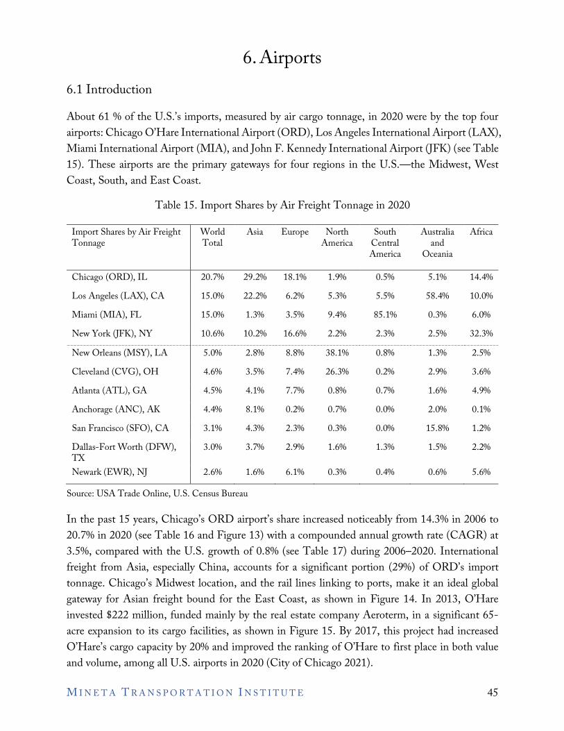
6. Airports 6.1 Introduction About 61 % of the U.S.’s imports, measured by air cargo tonnage, in 2020 were by the top four airports: Chicago O’Hare International Airport (ORD), Los Angeles International Airport (LAX), Miami International Airport (MIA), and John F. Kennedy International Airport (JFK) (see Table 15). These airports are the primary gateways for four regions in the U.S.—the Midwest, West Coast, South, and East Coast.
Table 15. Import Shares by Air Freight Tonnage in 2020
Import Shares by Air Freight Tonnage
Chicago (ORD), IL Los Angeles (LAX), CA Miami (MIA), FL New York (JFK), NY New Orleans (MSY), LA Cleveland (CVG), OH Atlanta (ATL), GA Anchorage (ANC), AK San Francisco (SFO), CA Dallas-Fort Worth (DFW), TX Newark (EWR), NJ
World Total
Asia Europe North America
South Central America
Australia and
Oceania
Africa
20.7% 29.2% 18.1% 1.9% 0.5% 5.1% 14.4% 15.0% 22.2% 6.2% 5.3% 5.5% 58.4% 10.0% 15.0% 1.3% 3.5% 9.4% 85.1% 0.3% 6.0% 10.6% 10.2% 16.6% 2.2% 2.3% 2.5% 32.3% 5.0% 2.8% 8.8% 38.1% 0.8% 1.3% 2.5% 4.6% 3.5% 7.4% 26.3% 0.2% 2.9% 3.6% 4.5% 4.1% 7.7% 0.8% 0.7% 1.6% 4.9% 4.4% 8.1% 0.2% 0.7% 0.0% 2.0% 0.1% 3.1% 4.3% 2.3% 0.3% 0.0% 15.8% 1.2% 3.0% 3.7% 2.9% 1.6% 1.3% 1.5% 2.2%
2.6% 1.6% 6.1% 0.3% 0.4% 0.6% 5.6%
Source: USA Trade Online, U.S. Census Bureau
In the past 15 years, Chicago’s ORD airport’s share increased noticeably from 14.3% in 2006 to 20.7% in 2020 (see Table 16 and Figure 13) with a compounded annual growth rate (CAGR) at 3.5%, compared with the U.S. growth of 0.8% (see Table 17) during 2006–2020. International freight from Asia, especially China, accounts for a significant portion (29%) of ORD’s import tonnage. Chicago’s Midwest location, and the rail lines linking to ports, make it an ideal global gateway for Asian freight bound for the East Coast, as shown in Figure 14. In 2013, O’Hare invested $222 million, funded mainly by the real estate company Aeroterm, in a significant 65-acre expansion to its cargo facilities, as shown in Figure 15. By 2017, this project had increased O’Hare’s cargo capacity by 20% and improved the ranking of O’Hare to first place in both value and volume, among all U.S. airports in 2020 (City of Chicago 2021).
M I N E T A T R A N S P O R T A T I O N I N S T I T U T E 45
Table 16. Import Shares of Air Freight Tonnage during 2006–2020
2006 2007 2008 2009 2010 2011 2012 2013 2014 2015 2016 2017 2018 2019 2020 Chicago (ORD), IL 14.3% 14.4% 14.7% 14.4% 15.7% 15.2% 14.9% 15.2% 16.9% 17.3% 16.1% 16.7% 16.8% 16.6% 20.7% Los Angeles (LAX), CA 13.2% 12.0% 11.5% 12.4% 12.2% 10.9% 11.7% 11.7% 12.2% 12.9% 12.9% 13.1% 12.9% 12.8% 15.0% Miami (MIA), FL 12.6% 12.7% 13.4% 14.7% 12.9% 13.5% 15.3% 16.1% 14.8% 14.2% 14.7% 13.3% 13.1% 13.8% 15.0% New York (JFK), NY 17.4% 16.1% 15.6% 14.9% 14.6% 14.2% 13.8% 13.8% 13.2% 13.2% 13.4% 13.1% 12.6% 12.7% 10.6% Atlanta (ATL), GA 5.5% 5.5% 5.2% 5.3% 5.6% 5.8% 5.3% 5.0% 4.9% 5.0% 5.1% 5.1% 5.0% 4.9% 4.5% San Francisco (SFO), CA 4.7% 4.7% 4.4% 4.0% 3.7% 3.4% 3.4% 3.3% 3.5% 3.8% 3.9% 4.1% 4.2% 4.1% 3.1%
Source: USA Trade Online, U.S. Census Bureau
Table 17. Growth of Air Freight Tonnage during 2006–2020
2006 2007 2008 2009 2010 2011 2012 2013 2014 2015 2016 2017 2018 2019 2020 CAGR Chicago (ORD), IL 1.1% 6.7% -9.7% -18.2% 37.1% -7.2% -4.7% 2.2% 21.6% 8.5% -8.8% 15.2% 5.6% -7.0% 22.5% 3.5% New York (JFK), NY 0.5% -2.3% -13.5% -20.2% 23.3% -7.6% -5.1% 0.1% 4.4% 5.9% -0.1% 7.9% 0.9% -4.0% -18.3% -2.6% Miami (MIA), FL -2.7% 6.0% -5.7% -9.0% 10.4% -0.3% 11.3% 5.2% 0.2% 1.5% 1.4% 0.4% 3.3% -0.1% 6.2% 2.1% Los Angeles (LAX), CA 2.6% -3.9% -14.7% -10.1% 23.5% -14.6% 4.7% 0.0% 14.0% 12.2% -2.2% 12.3% 4.1% -6.6% 15.1% 1.8% Atlanta (ATL), GA 7.3% 5.0% -16.0% -14.3% 32.1% 0.1% -11.6% -5.5% 8.0% 6.5% -0.2% 10.7% 4.0% -7.9% -10.2% -0.6% San Francisco (SFO), CA 8.5% 4.7% -15.5% -25.0% 15.9% -11.6% -3.4% -1.5% 16.8% 14.3% -0.2% 17.1% 7.4% -7.8% -25.8% -2.1% U.S. Total 2.8% 5.6% -11.0% -16.6% 25.9% -4.7% -2.2% 0.1% 9.1% 6.1% -2.2% 11.0% 5.0% -5.4% -2.0% 0.8%
Source: USA Trade Online, U.S. Census Bureau
M I N E T A T R A N S P O R T A T I O N I N S T I T U T E 46
20.0%
5.0%
0.0%
20.7%
New York
- Los Angeles
Atlanta 5.5% .... , :::::•:::::::=-------•------ e e e 4.5% e e -._._.___._ _____ _,.____.._ _____ ~•~----.J
e -------♦-• _.._. ------• _.____. • .___...,....._~ 4.7%
San Francisco 3.1%
2006 2007 2008 2009 2010 2011 2012 2013 2014 2015 2016 2017 2018 2019 2020
--Chicago (ORD), IL
..A-Miami (MIA), FL
--Atlanta (ATL), GA
--New York (JFK), NY
Los Angeles (LAX), CA
--San Francisco International Airport, CA
Figure 13. Trend of Import Shares of Air Freight Tonnage during 2006-2020
Source: USA Trade Online, U.S. Census Bureau
M I N E T A T R A N S P O R T A T I O N I N S T I T U T E 47
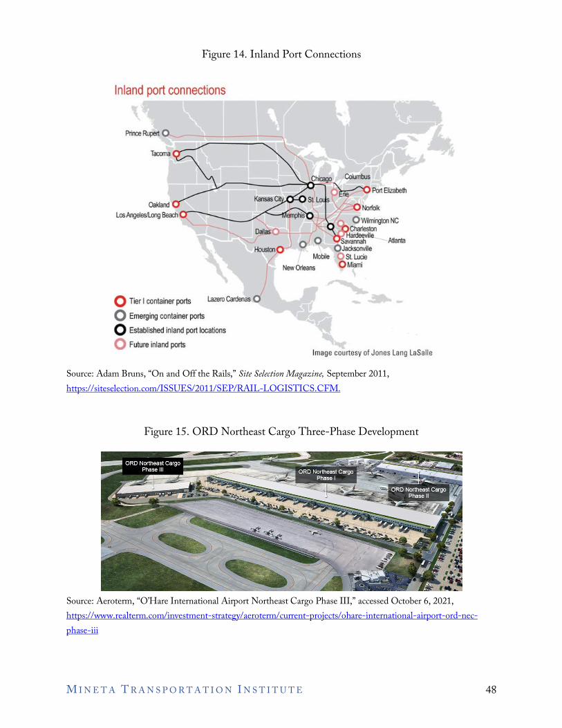
Inland port connections
Prn::e~O
Chicago. Columbus ,------___;~St..,_., ~ Pol!Elizabeth
LosAngelesA.ong Beach
Da1as
HoustonO
0Nolfak
Wlninglon NC
Allanla 6.Jad<somie
Mobie SL Lucie
New Orleans 0Miam
0 Tier I container ports Lazero Cardenas 0
0 Emerging container ports
0 Established inland port locations
0 Future inland ports Image courtesy of Jones Lang LaSalle
Figure 14. Inland Port Connections
Source: Adam Bruns, “On and Off the Rails,” Site Selection Magazine, September 2011, https://siteselection.com/ISSUES/2011/SEP/RAIL-LOGISTICS.CFM.
Figure 15. ORD Northeast Cargo Three-Phase Development
Source: Aeroterm, “O’Hare International Airport Northeast Cargo Phase III,” accessed October 6, 2021, https://www.realterm.com/investment-strategy/aeroterm/current-projects/ohare-international-airport-ord-nec-phase-iii
M I N E T A T R A N S P O R T A T I O N I N S T I T U T E 48
The Los Angeles LAX airport serves the Greater Los Angeles area, the second-largest metropolitan areas economically in the U.S. next to New York. Hence, LAX is a major international gateway for air cargo, ranked second nationally, and accounts for 15% of U.S. import air cargo tonnage (see Table 16) and passengers (second busiest passenger airport after Atlanta, GA). In addition, LAX is only 25 miles from the Ports of L.A. and L.B., which are among the top ports in the U.S. The close geographic locations of LAX and the Ports of L.A. and L.B. and linking highways and the rail freight system offer a tremendous potential opportunity for Southern California to become a strategic intermodal gateway to serve the entire U.S. market. However, LAX’s facilities are relatively old and very congested. The warehouses on site are not keeping up with the amount of cargo. There are significant road delays for trucks to load and unload. Though Los Angeles World Airports (LAWA) initiated the planning and development of over $14 billion in capital improvements at Los Angeles International Airport (LAX), this vast investment mainly focused on passenger operations, and the cargo areas were put on hold. In the past four decades, Ontario International airport (ONT), which is 55 miles to the east of LAX and surrounded by sufficient warehouse space and cheap land, has become an alternative for air cargo carriers. As a result, the share of LAX only slightly increased from 13.2% to 15% during 2006–2020 with a 1.8% CAGR (see Figure 13, Tables 16 and 17). Miami International airport (MIA) is an essential gateway for Latin America and handles 85% of freight from that region (see Table 16). The share of MIA has increased from 12.6% in 2006 to 15% in 2020 with a 2.1% CAGR (see Tables 16 and 17). DB Schenker (2019) indicates that MIA is one of the most innovative airports in several ways. First, MIA became one of the first six U.S. cargo hub airports to eliminate a paper air waybill and was designated by the U.S. Department of Commerce as a Foreign Trade Zone magnet site. Second, MIA established the first ocean-to-air perishables trans-shipment program in Florida and launched an internet-based real-time cargo flight tracker. Asia Cargo News recognized MIA as the 2018 Best Airport in North America for air cargo. New York’s JFK airport is ranked fourth on this list for import cargo volume by weight (see Table 16). The Newark airport (EWR) in NJ is nearby, and ranked 11th in the U.S. JFK, operated by the Port Authority of NY and NJ, benefits from its proximity to the Ports of NY and NJ, and access to an extensive East Coast/National rail network. The entire cargo area is designated as a free trade zone (FTZ) and is home to U.S. Customs for the Northeast region. In the past 15 years, JFK has lost market shares to competitors such as Chicago O’Hare airport (ORD). The share of JFK has dropped from 17.4% in 2006 to 10.6% in 2020 with a -2.6% CAGR (see Figure 13 and Tables 16and 17). Aging cargo facilities and chronic congestion along the Van Wyck Expressway, that brings trucks from JFK to Manhattan and the highways beyond, have been negatively affecting JFK’s competitiveness.
M I N E T A T R A N S P O R T A T I O N I N S T I T U T E 49
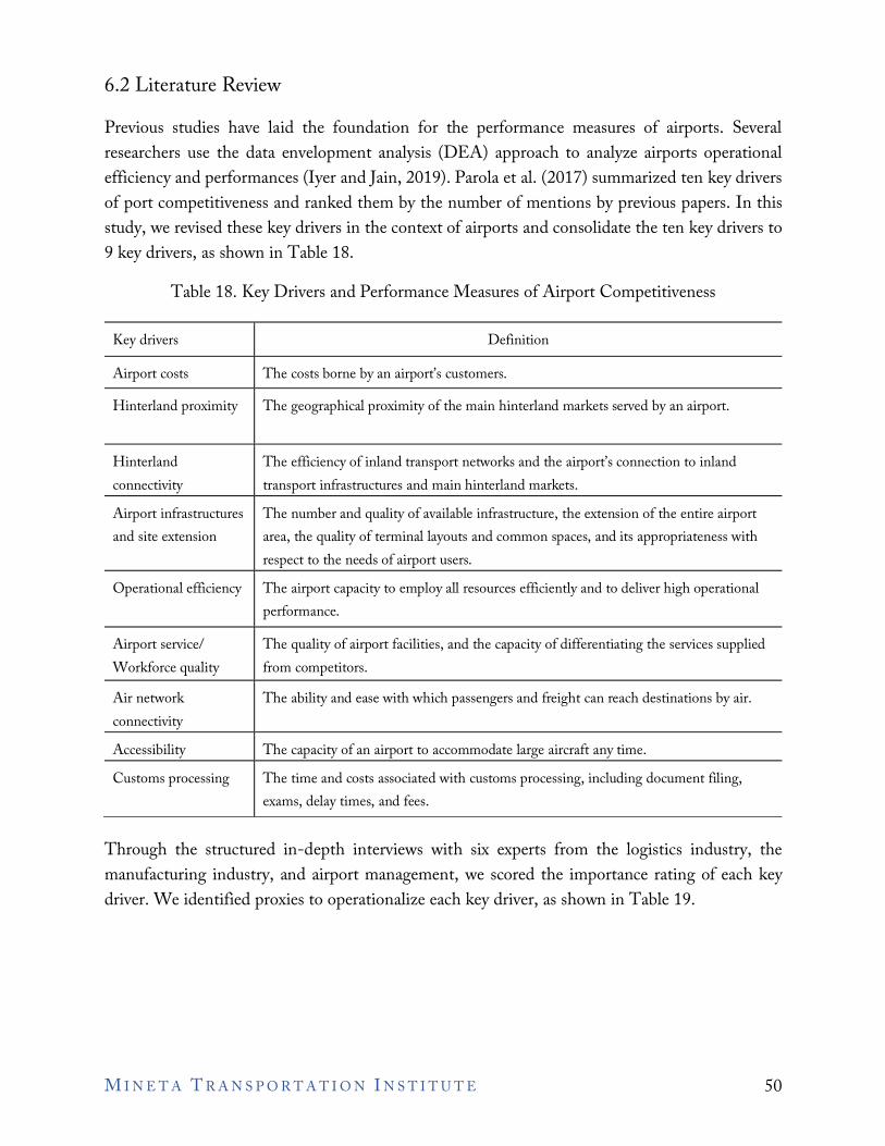
6.2 Literature Review Previous studies have laid the foundation for the performance measures of airports. Several researchers use the data envelopment analysis (DEA) approach to analyze airports operational efficiency and performances (Iyer and Jain, 2019). Parola et al. (2017) summarized ten key drivers of port competitiveness and ranked them by the number of mentions by previous papers. In this study, we revised these key drivers in the context of airports and consolidate the ten key drivers to 9 key drivers, as shown in Table 18.
Table 18. Key Drivers and Performance Measures of Airport Competitiveness
Key drivers Definition
Airport costs The costs borne by an airport’s customers.
Hinterland proximity The geographical proximity of the main hinterland markets served by an airport.
Hinterland connectivity
The efficiency of inland transport networks and the airport’s connection to inland transport infrastructures and main hinterland markets.
Airport infrastructures and site extension
The number and quality of available infrastructure, the extension of the entire airport area, the quality of terminal layouts and common spaces, and its appropriateness with respect to the needs of airport users.
Operational efficiency The airport capacity to employ all resources efficiently and to deliver high operational performance.
Airport service/ Workforce quality
The quality of airport facilities, and the capacity of differentiating the services supplied from competitors.
Air network connectivity
The ability and ease with which passengers and freight can reach destinations by air.
Accessibility The capacity of an airport to accommodate large aircraft any time. Customs processing The time and costs associated with customs processing, including document filing,
exams, delay times, and fees.
Through the structured in-depth interviews with six experts from the logistics industry, the manufacturing industry, and airport management, we scored the importance rating of each key driver. We identified proxies to operationalize each key driver, as shown in Table 19.
M I N E T A T R A N S P O R T A T I O N I N S T I T U T E 50
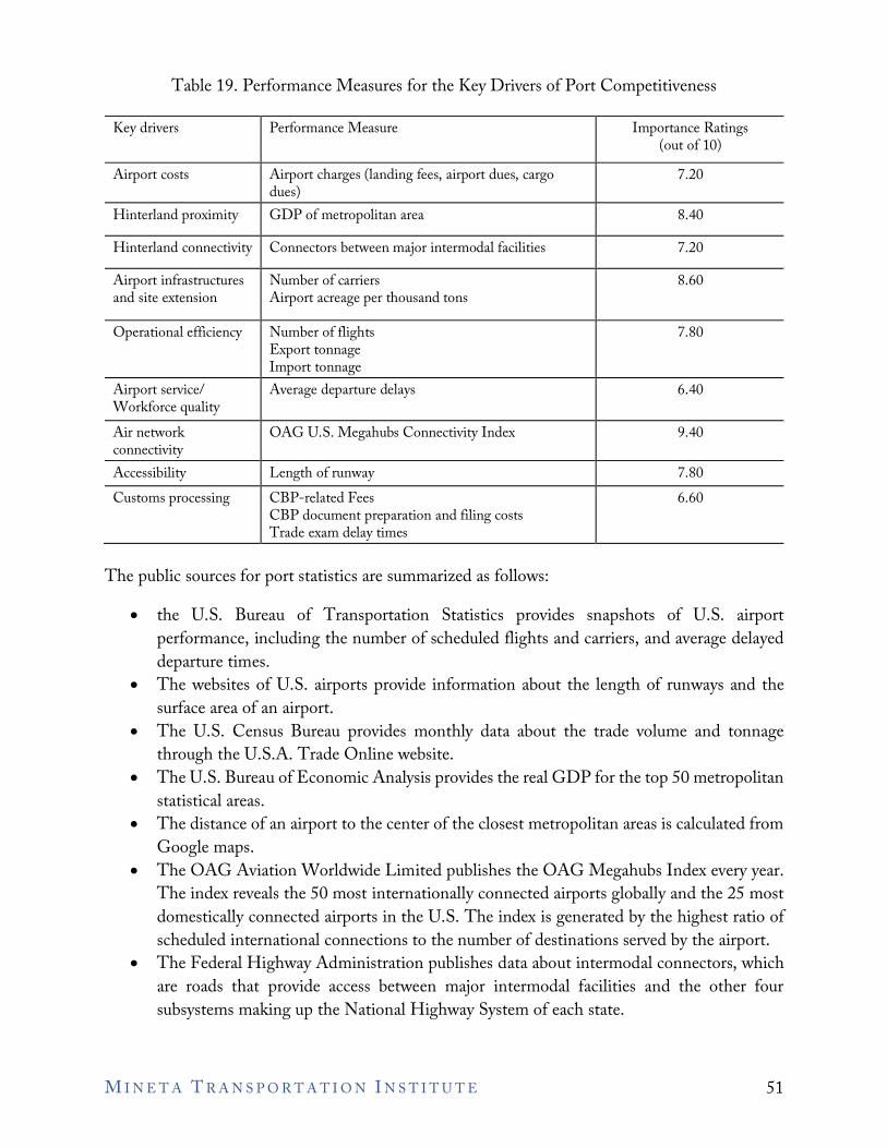
Table 19. Performance Measures for the Key Drivers of Port Competitiveness
Key drivers Performance Measure Importance Ratings (out of 10)
Airport costs Airport charges (landing fees, airport dues, cargo dues)
7.20
Hinterland proximity GDP of metropolitan area 8.40
Hinterland connectivity Connectors between major intermodal facilities 7.20
Airport infrastructures and site extension
Number of carriers Airport acreage per thousand tons
8.60
Operational efficiency Number of flights Export tonnage Import tonnage
7.80
Airport service/ Workforce quality
Average departure delays 6.40
Air network connectivity
OAG U.S. Megahubs Connectivity Index 9.40
Accessibility Length of runway 7.80 Customs processing CBP-related Fees
CBP document preparation and filing costs Trade exam delay times
6.60
The public sources for port statistics are summarized as follows:
• the U.S. Bureau of Transportation Statistics provides snapshots of U.S. airport performance, including the number of scheduled flights and carriers, and average delayed departure times.
• The websites of U.S. airports provide information about the length of runways and the surface area of an airport.
• The U.S. Census Bureau provides monthly data about the trade volume and tonnage through the U.S.A. Trade Online website.
• The U.S. Bureau of Economic Analysis provides the real GDP for the top 50 metropolitan statistical areas.
• The distance of an airport to the center of the closest metropolitan areas is calculated from Google maps.
• The OAG Aviation Worldwide Limited publishes the OAG Megahubs Index every year. The index reveals the 50 most internationally connected airports globally and the 25 most domestically connected airports in the U.S. The index is generated by the highest ratio of scheduled international connections to the number of destinations served by the airport.
• The Federal Highway Administration publishes data about intermodal connectors, which are roads that provide access between major intermodal facilities and the other four subsystems making up the National Highway System of each state.
M I N E T A T R A N S P O R T A T I O N I N S T I T U T E 51
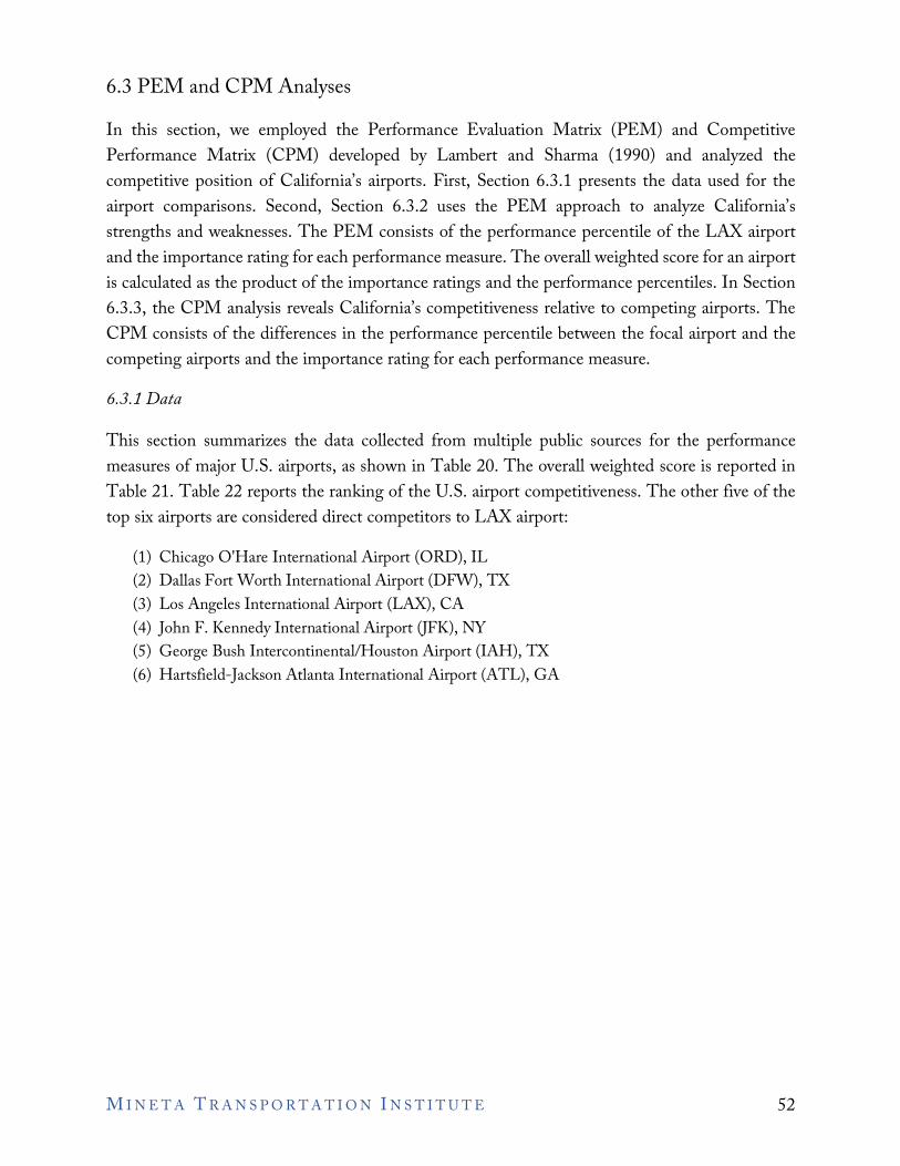
6.3 PEM and CPM Analyses In this section, we employed the Performance Evaluation Matrix (PEM) and Competitive Performance Matrix (CPM) developed by Lambert and Sharma (1990) and analyzed the competitive position of California’s airports. First, Section 6.3.1 presents the data used for the airport comparisons. Second, Section 6.3.2 uses the PEM approach to analyze California’s strengths and weaknesses. The PEM consists of the performance percentile of the LAX airport and the importance rating for each performance measure. The overall weighted score for an airport is calculated as the product of the importance ratings and the performance percentiles. In Section 6.3.3, the CPM analysis reveals California’s competitiveness relative to competing airports. The CPM consists of the differences in the performance percentile between the focal airport and the competing airports and the importance rating for each performance measure.
6.3.1 Data
This section summarizes the data collected from multiple public sources for the performance measures of major U.S. airports, as shown in Table 20. The overall weighted score is reported in Table 21. Table 22 reports the ranking of the U.S. airport competitiveness. The other five of the top six airports are considered direct competitors to LAX airport:
(1) Chicago O'Hare International Airport (ORD), IL (2) Dallas Fort Worth International Airport (DFW), TX (3) Los Angeles International Airport (LAX), CA (4) John F. Kennedy International Airport (JFK), NY (5) George Bush Intercontinental/Houston Airport (IAH), TX (6) Hartsfield-Jackson Atlanta International Airport (ATL), GA
M I N E T A T R A N S P O R T A T I O N I N S T I T U T E 52
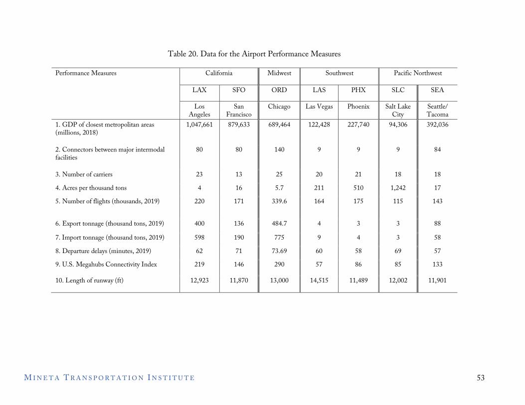
Table 20. Data for the Airport Performance Measures
Performance Measures California Midwest Southwest Pacific Northwest
LAX SFO ORD LAS PHX SLC SEA
Los Angeles
San Francisco
Chicago Las Vegas Phoenix Salt Lake City
Seattle/ Tacoma
1. GDP of closest metropolitan areas 1,047,661 879,633 689,464 122,428 227,740 94,306 392,036 (millions, 2018)
2. Connectors between major intermodal 80 80 140 9 9 9 84 facilities
3. Number of carriers 23 13 25 20 21 18 18 4. Acres per thousand tons 4 16 5.7 211 510 1,242 17 5. Number of flights (thousands, 2019) 220 171 339.6 164 175 115 143
6. Export tonnage (thousand tons, 2019) 400 136 484.7 4 3 3 88 7. Import tonnage (thousand tons, 2019) 598 190 775 9 4 3 58 8. Departure delays (minutes, 2019) 62 71 73.69 60 58 69 57 9. U.S. Megahubs Connectivity Index 219 146 290 57 86 85 133
10. Length of runway (ft) 12,923 11,870 13,000 14,515 11,489 12,002 11,901
M I N E T A T R A N S P O R T A T I O N I N S T I T U T E 53
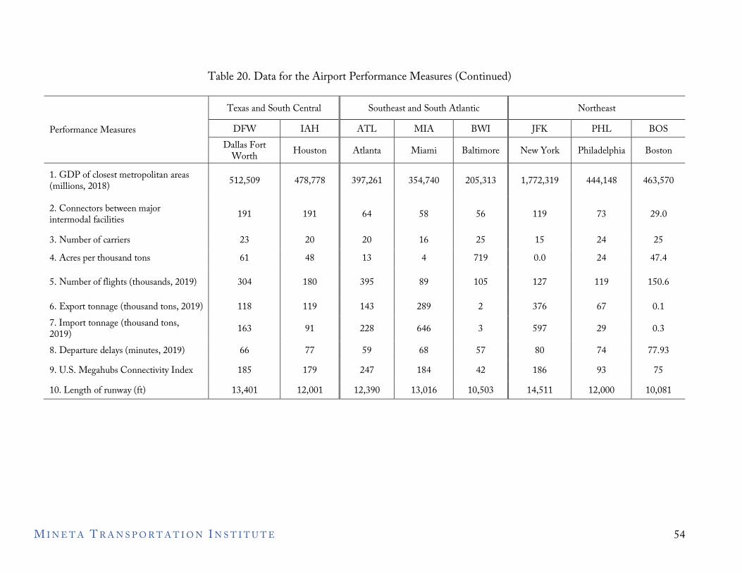
Table 20. Data for the Airport Performance Measures (Continued)
Performance Measures
Texas and South Central Southeast and South Atlantic Northeast DFW IAH ATL MIA BWI JFK PHL BOS
Dallas Fort Worth Houston Atlanta Miami Baltimore New York Philadelphia Boston
1. GDP of closest metropolitan areas (millions, 2018) 512,509 478,778 397,261 354,740 205,313 1,772,319 444,148 463,570
2. Connectors between major intermodal facilities 191 191 64 58 56 119 73 29.0
3. Number of carriers 23 20 20 16 25 15 24 25 4. Acres per thousand tons 61 48 13 4 719 0.0 24 47.4
5. Number of flights (thousands, 2019) 304 180 395 89 105 127 119 150.6
6. Export tonnage (thousand tons, 2019) 118 119 143 289 2 376 67 0.1 7. Import tonnage (thousand tons, 2019) 163 91 228 646 3 597 29 0.3
8. Departure delays (minutes, 2019) 66 77 59 68 57 80 74 77.93 9. U.S. Megahubs Connectivity Index 185 179 247 184 42 186 93 75 10. Length of runway (ft) 13,401 12,001 12,390 13,016 10,503 14,511 12,000 10,081
M I N E T A T R A N S P O R T A T I O N I N S T I T U T E 54
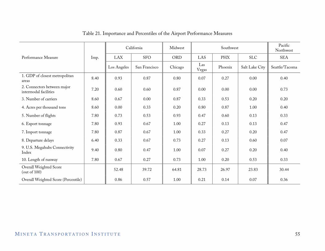
Table 21. Importance and Percentiles of the Airport Performance Measures
Performance Measure Imp.
California Midwest Southwest Pacific Northwest
LAX SFO ORD LAS PHX SLC SEA
Los Angeles San Francisco Chicago Las Vegas Phoenix Salt Lake City Seattle/Tacoma
1. GDP of closest metropolitan 8.40 0.93 0.87 0.80 0.07 0.27 0.00 0.40 areas 2. Connectors between major intermodal facilities 7.20 0.60 0.60 0.87 0.00 0.00 0.00 0.73
3. Number of carriers 8.60 0.67 0.00 0.87 0.33 0.53 0.20 0.20 4. Acres per thousand tons 8.60 0.00 0.33 0.20 0.80 0.87 1.00 0.40 5. Number of flights 7.80 0.73 0.53 0.93 0.47 0.60 0.13 0.33 6. Export tonnage 7.80 0.93 0.67 1.00 0.27 0.13 0.13 0.47 7. Import tonnage 7.80 0.87 0.67 1.00 0.33 0.27 0.20 0.47 8. Departure delays 6.40 0.33 0.67 0.73 0.27 0.13 0.60 0.07 9. U.S. Megahubs Connectivity Index 9.40 0.80 0.47 1.00 0.07 0.27 0.20 0.40
10. Length of runway 7.80 0.67 0.27 0.73 1.00 0.20 0.53 0.33 Overall Weighted Score (out of 100) Overall Weighted Score (Percentile)
52.48
0.86
39.72
0.57
64.81
1.00
28.73
0.21
26.97
0.14
23.83
0.07
30.44
0.36
M I N E T A T R A N S P O R T A T I O N I N S T I T U T E 55
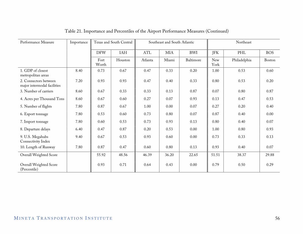
Table 21. Importance and Percentiles of the Airport Performance Measures (Continued)
Performance Measure Importance Texas and South Central Southeast and South Atlantic Northeast
DFW IAH ATL MIA BWI JFK PHL BOS Fort
Worth Houston Atlanta Miami Baltimore New
York Philadelphia Boston
1. GDP of closest metropolitan areas
8.40 0.73 0.67 0.47 0.33 0.20 1.00 0.53 0.60
2. Connectors between major intermodal facilities
7.20 0.93 0.93 0.47 0.40 0.33 0.80 0.53 0.20
3. Number of carriers 8.60 0.67 0.33 0.33 0.13 0.87 0.07 0.80 0.87 4. Acres per Thousand Tons 8.60 0.67 0.60 0.27 0.07 0.93 0.13 0.47 0.53 5. Number of flights 7.80 0.87 0.67 1.00 0.00 0.07 0.27 0.20 0.40 6. Export tonnage 7.80 0.53 0.60 0.73 0.80 0.07 0.87 0.40 0.00 7. Import tonnage 7.80 0.60 0.53 0.73 0.93 0.13 0.80 0.40 0.07 8. Departure delays 6.40 0.47 0.87 0.20 0.53 0.00 1.00 0.80 0.93 9. U.S. Megahubs Connectivity Index
9.40 0.67 0.53 0.93 0.60 0.00 0.73 0.33 0.13
10. Length of Runway 7.80 0.87 0.47 0.60 0.80 0.13 0.93 0.40 0.07 Overall Weighted Score
Overall Weighted Score (Percentile)
55.92
0.93
48.56
0.71
46.39
0.64
36.20
0.43
22.65
0.00
51.51
0.79
38.37
0.50
29.88
0.29
M I N E T A T R A N S P O R T A T I O N I N S T I T U T E 56
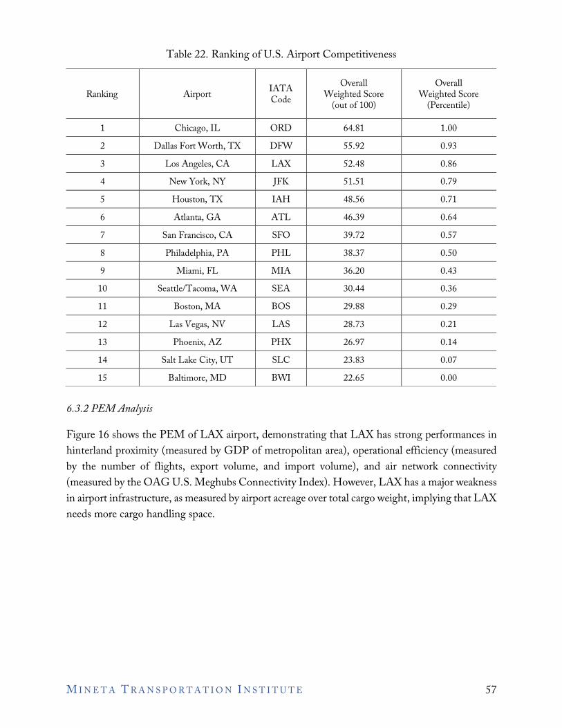
Table 22. Ranking of U.S. Airport Competitiveness
Ranking Airport IATA Code
Overall Weighted Score
(out of 100)
Overall Weighted Score
(Percentile)
1 Chicago, IL ORD 64.81 1.00 2 Dallas Fort Worth, TX DFW 55.92 0.93 3 Los Angeles, CA LAX 52.48 0.86 4 New York, NY JFK 51.51 0.79 5 Houston, TX IAH 48.56 0.71 6 Atlanta, GA ATL 46.39 0.64 7 San Francisco, CA SFO 39.72 0.57 8 Philadelphia, PA PHL 38.37 0.50 9 Miami, FL MIA 36.20 0.43
10 Seattle/Tacoma, WA SEA 30.44 0.36 11 Boston, MA BOS 29.88 0.29 12 Las Vegas, NV LAS 28.73 0.21 13 Phoenix, AZ PHX 26.97 0.14 14 Salt Lake City, UT SLC 23.83 0.07 15 Baltimore, MD BWI 22.65 0.00
6.3.2 PEM Analysis
Figure 16 shows the PEM of LAX airport, demonstrating that LAX has strong performances in hinterland proximity (measured by GDP of metropolitan area), operational efficiency (measured by the number of flights, export volume, and import volume), and air network connectivity (measured by the OAG U.S. Meghubs Connectivity Index). However, LAX has a major weakness in airport infrastructure, as measured by airport acreage over total cargo weight, implying that LAX needs more cargo handling space.
M I N E T A T R A N S P O R T A T I O N I N S T I T U T E 57
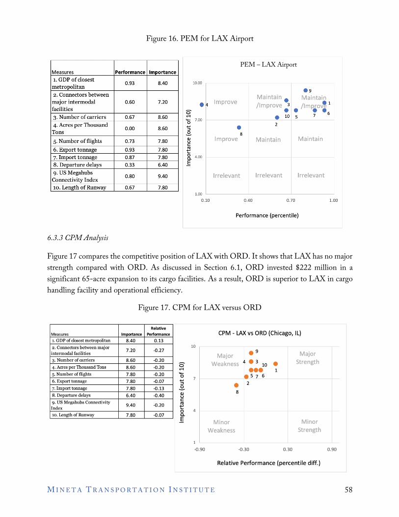
Measures Performance Importance
1. GDP of closest 0.93 8.40
metropolitan 2. Connectors between
major intermodal 0.60 7.20
facilities 3. Number of carriers 0.67 8.60
4. Acres per Thousand 0.00 8.60
Tons
10.00
.9
Improve Maintain• Maintain
• /Improve 3 /lmP.~ovt 1 0 • • .6 ...... • 10 5 7 - 7.00 0 2 .... • ::::,
.3. 8
5. Number of flights 0.73 7.80 (I) Improve Maintain Maintain u C:
6. Export tonnage 0.93 7.80 ro .... ... 7. Import tonnage 0.87 7.80
8. Departure delays 0.33 6.40
0 4.00 a. E
9. US Megahubs 0.80 9.40
Connectivity Index Irrelevant Irrelevant Irrelevant
10. Length of Runway 0.67 7.80 1.00
0.10 0.40 0.70 1.00
Performance (percentile}
Relative
Measures Importance Performance CPM - LAX vs ORD (Chicago, IL) 1. GDP of closest metropolitan 8.40 0.13 2. Connectors between major
7.20 --0.27 intermodal facilities 3. Number of carriers 8.60 --0.20 4. Acres per Thousand Tons 8.60 --0.20 5. Number of flights 7.80 --0.20 6. Export tonnage 7.80 --0.07 7. Import tonnage 7.80 --0.13 8. Departure delays 6.40 --0.40
10
Major .9 Major
0 Weakness 4 • 3 10 • Strength ...... • •• 1 -0 7 • 5 7 6 ..., :::, • 2 .3. QI 8 u
9. US Megahubs Connectivity 9.40 --0.20
Index
C: ro ..., ...
4 0 10. Length of Runway 7.80 --0.07 a.
E Minor Minor Weakness Strength
1
--0.90 -0.30 0.30 0.90
Relative Performance (percentile diff.)
Figure 16. PEM for LAX Airport
PEM – LAX Airport
6.3.3 CPM Analysis
Figure 17 compares the competitive position of LAX with ORD. It shows that LAX has no major strength compared with ORD. As discussed in Section 6.1, ORD invested $222 million in a significant 65-acre expansion to its cargo facilities. As a result, ORD is superior to LAX in cargo handling facility and operational efficiency.
Figure 17. CPM for LAX versus ORD
M I N E T A T R A N S P O R T A T I O N I N S T I T U T E 58
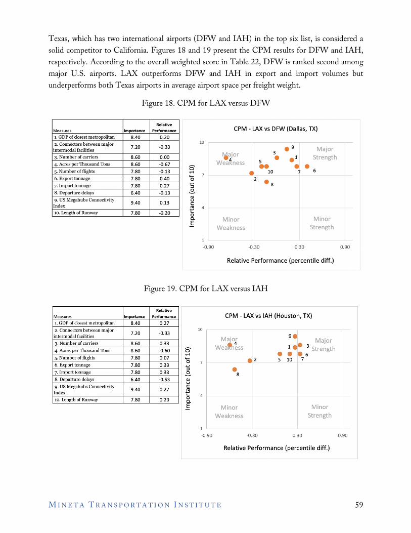
Relative Measures Importance Performance CPM - LAX vs DFW (Dallas, TX) 1. GDP of closest metropolitan 8.40 0.20 2. Connectors between major
7.20 -0.33 intermodal facilities 3. Number of carriers 8.60 0.00 4. Acres per Thousand Tons 8.60 -0.67 5. Number of flights 7.80 -0.13 6. Export tonnage 7.80 0.40 7. Import tonnage 7.80 0.27
10
3 .9 Major
~ajor 5 • .1 Strength
Wea ness 0 •• • • .-t • 10 7 6 ..... 7 0 2
•8 .., ::,
8. Departure delays 6.40 -0.13 .£. 9. US Megahubs Connectivity
9.40 0.13 Index 10. Length of Runway 7.80 -0.20
QJ u C: ro 4 .., ... 0 a. Minor Minor E
Weakness Strength
1
-0.90 -0.30 0.30 0.90
Relative Performance (percentile diff.)
Relative Measures Importance Performance CPM - LAX vs IAH (Houston, TX) 1. GDP of closest metropolitan 8.40 0.27 2. Connectors between major
7.20 -0.33 intermodal facilities 3. Number of carriers 8.60 0.33
4. Acres per Thousand Tons 8.60 -0.60
5. Number of flights 7.80 0.07 6. Export tonnage 7.80 0.33 7. Im port tonnage 7.80 0.33
10
Major 9. Major
0 Wea~~ss 1 e• 3 Strength
.-t • • • 6 ..... .2 5 10 7 0 7 .., ::, • .£. 8
8. Departure delays 6.40 -0.53 QJ u
9. US Megahubs Connectivity 9.40 0.27
Index 10. Length of Runway 7.80 0.20
C: ro .., ... 4 0 a. E Minor Minor
Weakness Strength
1
-0.90 -0.30 0.30 0.90
Relative Performance (percentile diff.)
Texas, which has two international airports (DFW and IAH) in the top six list, is considered a solid competitor to California. Figures 18 and 19 present the CPM results for DFW and IAH, respectively. According to the overall weighted score in Table 22, DFW is ranked second among major U.S. airports. LAX outperforms DFW and IAH in export and import volumes but underperforms both Texas airports in average airport space per freight weight.
Figure 18. CPM for LAX versus DFW
Figure 19. CPM for LAX versus IAH
M I N E T A T R A N S P O R T A T I O N I N S T I T U T E 59
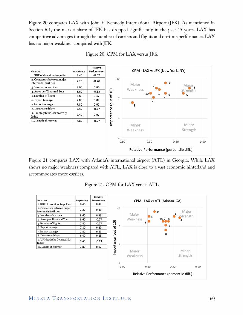
Relative Measures Importance Performance CPM - LAX vs JFK (New York, NY) 1. GDP of closest metropolitan 8.40 -0.07
2. Connectors between major 7.20 -0.20
intermodal facilities
3. Number of carriers 8.60 0.60
4. Acres per Thousand Tons 8.60 -0.13
5. Number of flights 7.80 0.47
6. Export tonnage 7.80 0.07
7. Im port tonnage 7.80 0.07
10
Major • 9 Ma~or3 4.
0 Weakness • Strength .-t 10• 1 .6 •s .... 0
7 • 7 .... 2 :, • 0
8 8. Departure delays 6.40 -0.67 QJ
u 9. US Megahubs Connectivity
9.40 0.07 Index
10. Length of Runway 7.80 -0.27
C ro .... ....
4 0 a. E Minor Minor
Weakness Strength
1
-0.90 -0.30 0.30 0.90
Relative Performance (percentile diff.)
Relative
Measures Importance Performance
1. GDP of closest metropolitan 8.40 0.47 CPM - LAX vs ATL (Atlanta, GA}
2. Connectors between major 7.20 0.13
intermodal facilities 3. Number of carriers 8.60 0.33 4. Acres per Thousand Tons 8.60 -0.27 5. Number of flights 7.80 -0.27 6. Export tonnage 7.80 0.20 7. Import tonnage 7.80 0.13 8. Departure delays 6.40 0.13
10
.9 Major Major 1
.4 • e5trength
0 Weakness
s• 1~~4i 3 .-t • - 7 2 0 • .... :,
~ 8
9. US Megahubs Connectivity 9.40 -0.13
Index 10. Length of Runway 7.80 0.07
QJ u C ro 4 t 0 C. Minor Minor E
Weakness Strength
-0.90 -0.30 0.30 0.90
Relative Performance (percentile diff.)
Figure 20 compares LAX with John F. Kennedy International Airport (JFK). As mentioned in Section 6.1, the market share of JFK has dropped significantly in the past 15 years. LAX has competitive advantages through the number of carriers and flights and on-time performance. LAX has no major weakness compared with JFK.
Figure 20. CPM for LAX versus JFK
Figure 21 compares LAX with Atlanta’s international airport (ATL) in Georgia. While LAX shows no major weakness compared with ATL, LAX is close to a vast economic hinterland and accommodates more carriers.
Figure 21. CPM for LAX versus ATL
M I N E T A T R A N S P O R T A T I O N I N S T I T U T E 60
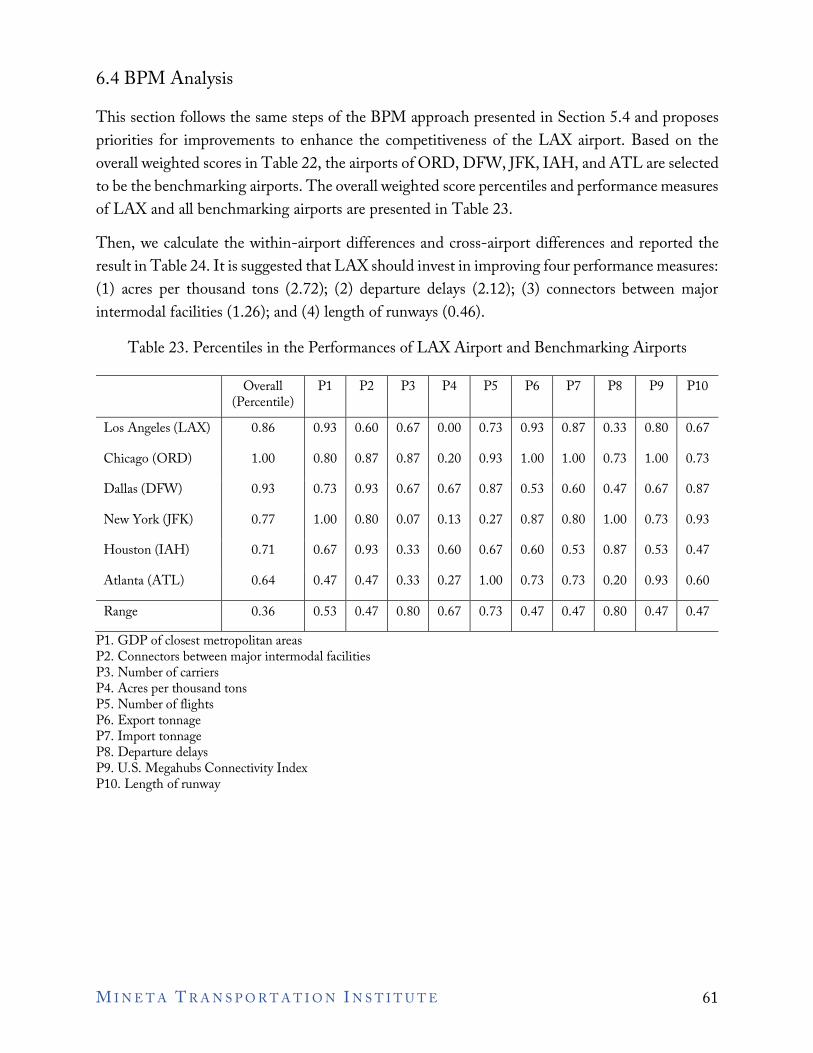
6.4 BPM Analysis This section follows the same steps of the BPM approach presented in Section 5.4 and proposes priorities for improvements to enhance the competitiveness of the LAX airport. Based on the overall weighted scores in Table 22, the airports of ORD, DFW, JFK, IAH, and ATL are selected to be the benchmarking airports. The overall weighted score percentiles and performance measures of LAX and all benchmarking airports are presented in Table 23. Then, we calculate the within-airport differences and cross-airport differences and reported the result in Table 24. It is suggested that LAX should invest in improving four performance measures: (1) acres per thousand tons (2.72); (2) departure delays (2.12); (3) connectors between major intermodal facilities (1.26); and (4) length of runways (0.46).
Table 23. Percentiles in the Performances of LAX Airport and Benchmarking Airports
Overall (Percentile)
P1 P2 P3 P4 P5 P6 P7 P8 P9 P10
Los Angeles (LAX) 0.86 0.93 0.60 0.67 0.00 0.73 0.93 0.87 0.33 0.80 0.67
Chicago (ORD) 1.00 0.80 0.87 0.87 0.20 0.93 1.00 1.00 0.73 1.00 0.73
Dallas (DFW) 0.93 0.73 0.93 0.67 0.67 0.87 0.53 0.60 0.47 0.67 0.87
New York (JFK) 0.77 1.00 0.80 0.07 0.13 0.27 0.87 0.80 1.00 0.73 0.93
Houston (IAH) 0.71 0.67 0.93 0.33 0.60 0.67 0.60 0.53 0.87 0.53 0.47
Atlanta (ATL) 0.64 0.47 0.47 0.33 0.27 1.00 0.73 0.73 0.20 0.93 0.60
Range 0.36 0.53 0.47 0.80 0.67 0.73 0.47 0.47 0.80 0.47 0.47 P1. GDP of closest metropolitan areas P2. Connectors between major intermodal facilities P3. Number of carriers P4. Acres per thousand tons P5. Number of flights P6. Export tonnage P7. Import tonnage P8. Departure delays P9. U.S. Megahubs Connectivity Index P10. Length of runway
M I N E T A T R A N S P O R T A T I O N I N S T I T U T E 61
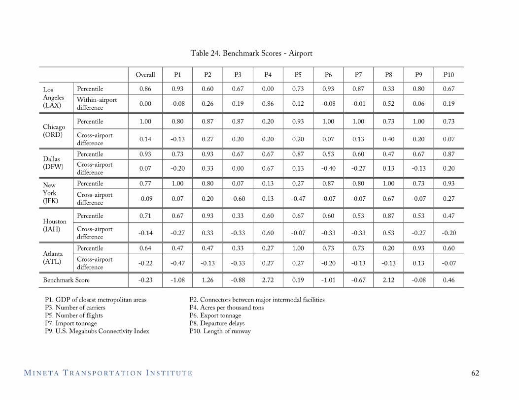
Table 24. Benchmark Scores - Airport
Overall P1 P2 P3 P4 P5 P6 P7 P8 P9 P10
Los Angeles (LAX)
Percentile 0.86 0.93 0.60 0.67 0.00 0.73 0.93 0.87 0.33 0.80 0.67 Within-airport difference 0.00 -0.08 0.26 0.19 0.86 0.12 -0.08 -0.01 0.52 0.06 0.19
Chicago (ORD)
Percentile 1.00 0.80 0.87 0.87 0.20 0.93 1.00 1.00 0.73 1.00 0.73 Cross-airport difference 0.14 -0.13 0.27 0.20 0.20 0.20 0.07 0.13 0.40 0.20 0.07
Dallas (DFW)
Percentile 0.93 0.73 0.93 0.67 0.67 0.87 0.53 0.60 0.47 0.67 0.87 Cross-airport difference 0.07 -0.20 0.33 0.00 0.67 0.13 -0.40 -0.27 0.13 -0.13 0.20
New York (JFK)
Percentile 0.77 1.00 0.80 0.07 0.13 0.27 0.87 0.80 1.00 0.73 0.93 Cross-airport difference -0.09 0.07 0.20 -0.60 0.13 -0.47 -0.07 -0.07 0.67 -0.07 0.27
Houston (IAH)
Percentile 0.71 0.67 0.93 0.33 0.60 0.67 0.60 0.53 0.87 0.53 0.47 Cross-airport difference -0.14 -0.27 0.33 -0.33 0.60 -0.07 -0.33 -0.33 0.53 -0.27 -0.20
Atlanta (ATL)
Percentile 0.64 0.47 0.47 0.33 0.27 1.00 0.73 0.73 0.20 0.93 0.60 Cross-airport difference -0.22 -0.47 -0.13 -0.33 0.27 0.27 -0.20 -0.13 -0.13 0.13 -0.07
Benchmark Score -0.23 -1.08 1.26 -0.88 2.72 0.19 -1.01 -0.67 2.12 -0.08 0.46
P1. GDP of closest metropolitan areas P2. Connectors between major intermodal facilities P3. Number of carriers P4. Acres per thousand tons P5. Number of flights P6. Export tonnage P7. Import tonnage P8. Departure delays P9. U.S. Megahubs Connectivity Index P10. Length of runway
M I N E T A T R A N S P O R T A T I O N I N S T I T U T E 62
6.5 Comments from Interviews The above quantitative analysis was complemented with a qualitative discussion of interviewee responses to open-ended questions. For example, experts were asked about data and measures of airport competitiveness, the current and future state of California’s airport competitiveness, and related environmental impact, sustainability, and resilience issues.
6.5.1 Data and measures
Experts suggested that labor costs, storage fees, destroy cargo fees, screening fees, and processing speed be considered airport costs. Regarding hinterland connectivity, experts suggested adding congestion at airports as a performance measure. In addressing operational efficiency, experts suggested adding the amount of landing and takeoffs, in-and-out speed, security, and processing speed as performance measures. For airport service quality, experts suggest adding average lag time between flight arrival and freight delivery, and the availability of different levels of service—e.g., general versus express, and temperature/ refrigeration facilities. Finally, regarding accessibility, experts suggested considering aircraft ground handling equipment.
6.5.2 Current State of California freight competitiveness
Experts indicated that California’s main competitors included Houston, Midwest, New York, Atlanta, and Washington. Tijuana in Mexico could be a potential competitor in the future. Experts recognized that California has made the following investments:
• Better transportation systems and more terminal services. • K9 screening. • Capacity improvements to increase speed and space at airports. • Increasing capacity for handing large aircrafts. • Increasing people mover capacity. • LAX spent $16 billion on the passenger side but nothing on cargo, especially for freight
handling.
About the bottlenecks in California’s airport system, experts mentioned several constraints of LAX airport. First, LAX buildings are old and small and have no space for expansion. Second, many trucks line up in a queue and are slow to load. There is no software to move trucks faster. There is software for the appointment system, and the dispatcher can select an appointment time for check-in. However, only Mercury Handling Company has adopted this approach. Third, there is a significant lack of drivers. It is difficult to get good drivers because they require a TSA background check. Long hauls offer $10k signing bonuses. It requires $2k to get a Class A license and a driver needs 2 years of experience due to insurance. The turnover for drivers is very high because they don’t want to deal with the airport as it requires waiting in long lines.
M I N E T A T R A N S P O R T A T I O N I N S T I T U T E 63
Fourth, airports do not employ enough people to move the freight quickly enough. As a result, airline companies partner with handling companies. Handling companies cannot afford to employ the workforce, but need to, and thus take on the risk.
6.5.3 The future of California’s freight competitiveness
Experts indicated some threats faced by California. First, companies are leaving California to other states such as Texas. Inland airports, like Chicago and Dallas, keep improving efficiency and enhancing their competitiveness. Tijuana, Mexico may become a potential threat if firms can handle cargo there. Experts proposed some suggestions to make LAX more competitive:
• Airlines should have more control over when planes come in and out of LAX. • LAX should improve infrastructure and operational efficiency. • LAX should expand freight handling facilities and use technology to reduce trucking dwell
time. • The price charged by LAX has to be fair and based on market value.
Experts advised that California invest in more routes, better trucks, higher speed, and increased freight handling infrastructure. The government needs to improve highways and reduce congestion. California needs to revise the airport security/background checks procedure so that truck drivers can get approved faster. LAX should add a train line to handle cargo from the aircraft, and build up systems to process more freight.
6.6 Port Performance with respect to the Environment, Sustainability, and Resilience
Most experts indicated that the LAX airport is very resilient to disasters, outages or accidents, and economic downturns in terms of having policies, contingency plans, and quick response to disasters. Airports may negatively affect the environment in the following ways:
• Fossil fuel usage. • Global warming. • Air pollution from planes and trucks. • Fuel price rising from banning fracking. • Airline fuel impacts to wildlife around the airport. • Aircraft noises.
Experts suggested that airports should use more biofuel rather than fossil fuel, use more solar energy, and require clean air trucks to minimize the negative impact. More electrical charging stations are needed in the airport facilities. Airports can increase fees for polluting vehicles.
M I N E T A T R A N S P O R T A T I O N I N S T I T U T E 64
Government should invest in trains and sustainability programs, and run a program to handle wildlife around the airports.
6.7 Conclusion 6.7.1 Findings
The PEM and CPM approaches identified the strengths, the weaknesses, and the competitive position of LAX. On the one hand, LAX has strong performances in hinterland proximity (measured by GDP of metropolitan area), operational efficiency (measured by the number of flights, export and import volumes), and air network connectivity (measured by OAG Meghubs Connectivity Index). However, on the other hand, LAX has a major weakness in terms of airport infrastructure measured by airport acreage over total cargo weight, implying that LAX needs more cargo handling space. Based on the overall weighted scores, ORD, DFW, JFK, IAH, and ATL airports are considered direct competitors to LAX airport in California. For the BPM analysis, it is suggested that the state prioritize investment in the space of cargo handling facilities, departure delays, the intermodal connection between airports and other transport modes, and length of runways. Experts called for more investment in cargo handling facilities when considering the current state of California airport competitiveness, due to the limited room for expansion. Inland airports like Chicago and Dallas keep improving efficiency and enhancing competitiveness. In addition, there is a significant lack of truck drivers because of long trucking dwell time and the complex procedures for airport security/background checks. The airport could use more technology to reduce trucking dwell time.
6.7.2 Suggestions
Los Angeles World Airports (LAWA) has initiated the planning and development of over $14 billion in capital improvements at Los Angeles International Airport (LAX), projected to last through 2023. However, this vast investment mainly focused on passenger operations, and LAWA decided to put the cargo project on hold. The cargo handling facilities and warehouses are crowded and obsolete, requiring significant modernization. In addition, expanding cargo capacity at LAX is challenging as the airport does not have any idle space to relocate operations. LAX needs to introduce new technology to address the cargo backlogs and congestion at the airport. For example, Mercury Air Cargo has been testing an online appointment system to verify Customs clearance, check cargo availability, electronic pay terminal handling fees, and reserve a dock door (Kulisch 2019). In addition, Southern California’s emerging airports in the Inland Empire, including Ontario International (ONT), San Bernardino International Airport (SBD), and March Air Reserve Base
M I N E T A T R A N S P O R T A T I O N I N S T I T U T E 65
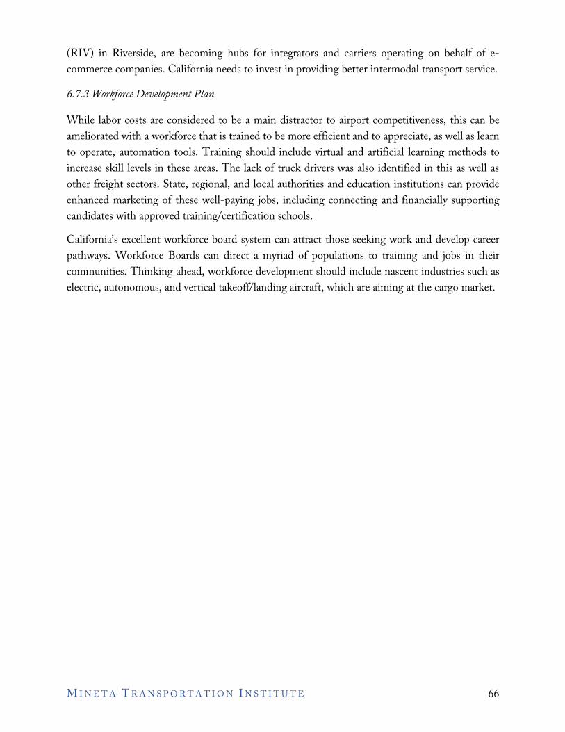
(RIV) in Riverside, are becoming hubs for integrators and carriers operating on behalf of e-commerce companies. California needs to invest in providing better intermodal transport service.
6.7.3 Workforce Development Plan
While labor costs are considered to be a main distractor to airport competitiveness, this can be ameliorated with a workforce that is trained to be more efficient and to appreciate, as well as learn to operate, automation tools. Training should include virtual and artificial learning methods to increase skill levels in these areas. The lack of truck drivers was also identified in this as well as other freight sectors. State, regional, and local authorities and education institutions can provide enhanced marketing of these well-paying jobs, including connecting and financially supporting candidates with approved training/certification schools. California’s excellent workforce board system can attract those seeking work and develop career pathways. Workforce Boards can direct a myriad of populations to training and jobs in their communities. Thinking ahead, workforce development should include nascent industries such as electric, autonomous, and vertical takeoff/landing aircraft, which are aiming at the cargo market.
M I N E T A T R A N S P O R T A T I O N I N S T I T U T E 66
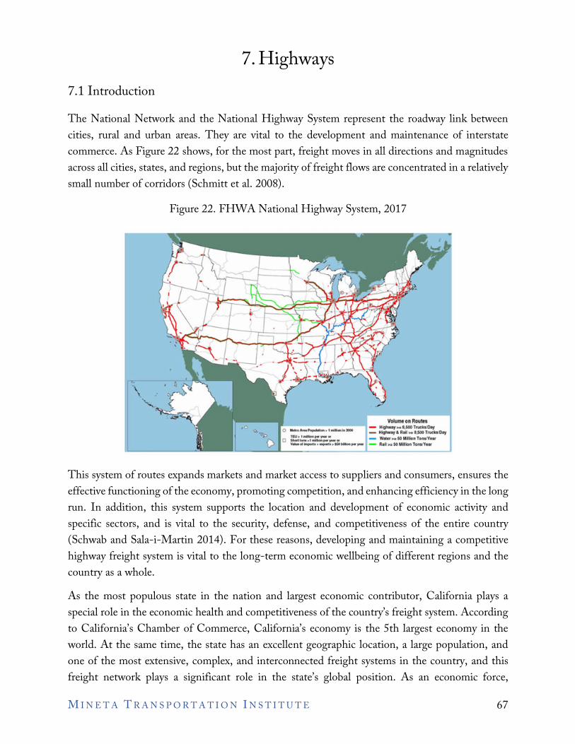
·-.
Volumf: on Routtt - Hlpty >a 1,500 Ttt;iCb:0.,,,
rw~, ...... ,.... - Wtlff>11$0MillirMITOMIYMf - HiQtlw..,lAall.-UOOTMb/Oay I
0 ==--~~:-:.;._..,__ - Aall,dOMllllot1T-1Y-
7. Highways 7.1 Introduction The National Network and the National Highway System represent the roadway link between cities, rural and urban areas. They are vital to the development and maintenance of interstate commerce. As Figure 22 shows, for the most part, freight moves in all directions and magnitudes across all cities, states, and regions, but the majority of freight flows are concentrated in a relatively small number of corridors (Schmitt et al. 2008).
Figure 22. FHWA National Highway System, 2017
This system of routes expands markets and market access to suppliers and consumers, ensures the effective functioning of the economy, promoting competition, and enhancing efficiency in the long run. In addition, this system supports the location and development of economic activity and specific sectors, and is vital to the security, defense, and competitiveness of the entire country (Schwab and Sala-i-Martin 2014). For these reasons, developing and maintaining a competitive highway freight system is vital to the long-term economic wellbeing of different regions and the country as a whole. As the most populous state in the nation and largest economic contributor, California plays a special role in the economic health and competitiveness of the country’s freight system. According to California’s Chamber of Commerce, California’s economy is the 5th largest economy in the world. At the same time, the state has an excellent geographic location, a large population, and one of the most extensive, complex, and interconnected freight systems in the country, and this freight network plays a significant role in the state’s global position. As an economic force,
M I N E T A T R A N S P O R T A T I O N I N S T I T U T E 67
California’s freight network connects the state to the rest of the country and the world. California’s core freight system includes approximately 5,800 miles of high traffic volume interstate and state highways, among other essential components like ports and airports (see Figure 23). To put this states’ economic contributions in context, California exported to 230 foreign economies in 2019. Its exports were valued at approximately $178 billion, up from $172 billion in 2017 and $163.5 billion in 2016 (California Chamber of Commerce 2018, 2019). According to the Bureau of Transportation Statistics, the freight system also facilitates commerce internally. In 2015, shipments within the state comprised 62% of all California shipments. It is also forecasted that by 2040, California’s highway system will carry more than 1.2 billion tons of freight annually, valued at $1.9 trillion—a 26 % by tonnage, and 52 % by value, increase from 2015.
Figure 23. California Freight Network: California Mobility Plan 2020
As the leading national gateway for international trade and domestic commerce, California exemplifies the world’s most innovative, economically competitive, multimodal freight network that is efficient, reliable, modern, integrated, resilient, safe, and sustainable, where social and environmental impacts are considered equally (California Freight Mobility Plan 2020).
M I N E T A T R A N S P O R T A T I O N I N S T I T U T E 68
7.2 Literature Review In order to maintain and enhance their competitive performance, most states rely on a long list of highway freight performance measures. In 1993, the federal government passed the Performance and Results Act that requires all federal agencies to develop, maintain, and use performance measures (McMullen and Monsere 2010). In addition, the Act requires the development of strategic plans, annual performance plans, and annual performance reports. At the same time, most states have passed mandates that require the development of similar performance measures at the state level. Accordingly, several state transportation agencies have been using performance measures for several years (Poister 2004). The Federal Highway Administration (FHWA) Office of Freight Management and Operations is responsible for administering freight performance measurement requirements as outlined in the Moving Ahead for Progress in the 21st Century (MAP-21) and the Fixing America’s Surface Transportation (FAST) Act (Easley et al. 2017). The FHWA assists developing freight performance measures through the advancement and dissemination of freight data and tools, to support appropriate analysis, plans, and project development. FHWA developed the Freight Performance Measure Primer as a tool for state departments of transportation (DOTs) and Metropolitan Planning Organizations (MPOs) to develop meaningful, effective, and consistent performance measurement practices (U.S. Department of Transportation, Freight Performance Measure Primer). In terms of the highway system’s performance measures, Primer’s highway freight performance measures fall in the categories of safety, maintenance and preservation, mobility, reliability, congestion, accessibility and connectivity, and environment (see Table 25).
M I N E T A T R A N S P O R T A T I O N I N S T I T U T E 69
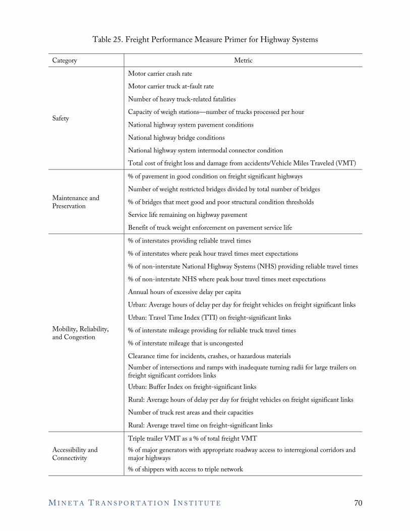
Table 25. Freight Performance Measure Primer for Highway Systems
Category Metric
Safety
Motor carrier crash rate Motor carrier truck at-fault rate Number of heavy truck-related fatalities Capacity of weigh stations—number of trucks processed per hour National highway system pavement conditions National highway bridge conditions National highway system intermodal connector condition Total cost of freight loss and damage from accidents/Vehicle Miles Traveled (VMT)
Maintenance and Preservation
% of pavement in good condition on freight significant highways Number of weight restricted bridges divided by total number of bridges % of bridges that meet good and poor structural condition thresholds Service life remaining on highway pavement Benefit of truck weight enforcement on pavement service life
Mobility, Reliability, and Congestion
% of interstates providing reliable travel times % of interstates where peak hour travel times meet expectations % of non-interstate National Highway Systems (NHS) providing reliable travel times % of non-interstate NHS where peak hour travel times meet expectations Annual hours of excessive delay per capita Urban: Average hours of delay per day for freight vehicles on freight significant links Urban: Travel Time Index (TTI) on freight-significant links % of interstate mileage providing for reliable truck travel times % of interstate mileage that is uncongested Clearance time for incidents, crashes, or hazardous materials Number of intersections and ramps with inadequate turning radii for large trailers on freight significant corridors links Urban: Buffer Index on freight-significant links Rural: Average hours of delay per day for freight vehicles on freight significant links Number of truck rest areas and their capacities Rural: Average travel time on freight-significant links
Accessibility and Connectivity
Triple trailer VMT as a % of total freight VMT % of major generators with appropriate roadway access to interregional corridors and major highways % of shippers with access to triple network
M I N E T A T R A N S P O R T A T I O N I N S T I T U T E 70
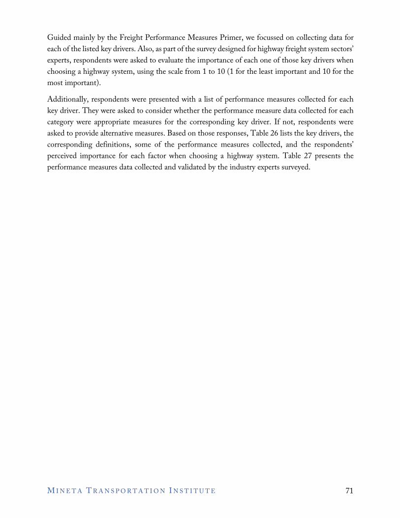
Guided mainly by the Freight Performance Measures Primer, we focussed on collecting data for each of the listed key drivers. Also, as part of the survey designed for highway freight system sectors’ experts, respondents were asked to evaluate the importance of each one of those key drivers when choosing a highway system, using the scale from 1 to 10 (1 for the least important and 10 for the most important). Additionally, respondents were presented with a list of performance measures collected for each key driver. They were asked to consider whether the performance measure data collected for each category were appropriate measures for the corresponding key driver. If not, respondents were asked to provide alternative measures. Based on those responses, Table 26 lists the key drivers, the corresponding definitions, some of the performance measures collected, and the respondents’ perceived importance for each factor when choosing a highway system. Table 27 presents the performance measures data collected and validated by the industry experts surveyed.
M I N E T A T R A N S P O R T A T I O N I N S T I T U T E 71
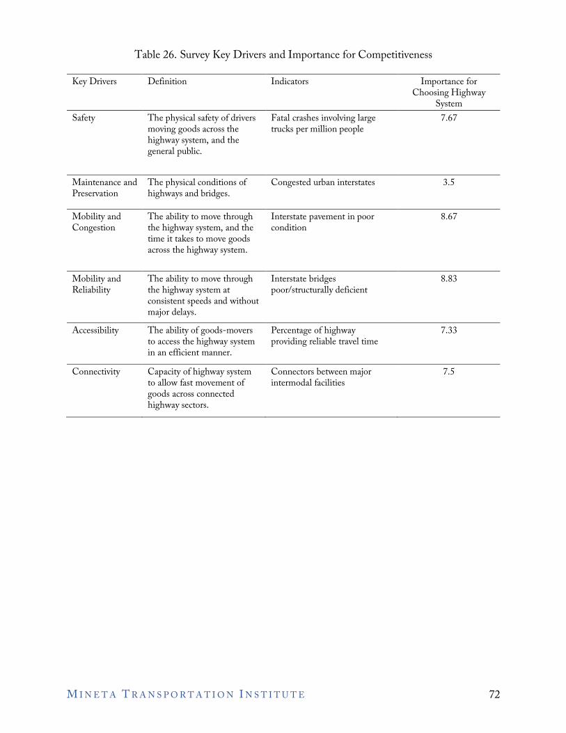
Table 26. Survey Key Drivers and Importance for Competitiveness
Key Drivers Definition Indicators Importance for Choosing Highway
System Safety The physical safety of drivers
moving goods across the highway system, and the general public.
Fatal crashes involving large trucks per million people
7.67
Maintenance and Preservation
The physical conditions of highways and bridges.
Congested urban interstates 3.5
Mobility and Congestion
The ability to move through the highway system, and the time it takes to move goods across the highway system.
Interstate pavement in poor condition
8.67
Mobility and Reliability
The ability to move through the highway system at consistent speeds and without major delays.
Interstate bridges poor/structurally deficient
8.83
Accessibility The ability of goods-movers to access the highway system in an efficient manner.
Percentage of highway providing reliable travel time
7.33
Connectivity Capacity of highway system to allow fast movement of
Connectors between major intermodal facilities
7.5
goods across connected highway sectors.
M I N E T A T R A N S P O R T A T I O N I N S T I T U T E 72
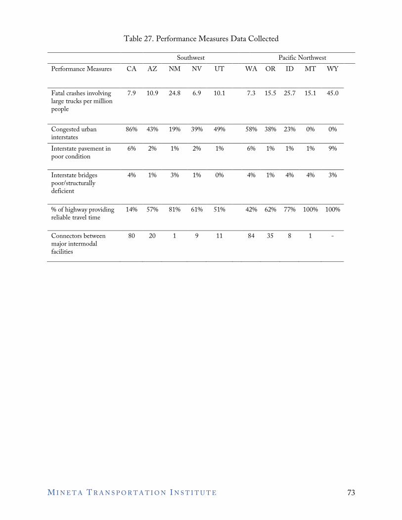
Table 27. Performance Measures Data Collected
Southwest Pacific Northwest Performance Measures CA AZ NM NV UT WA OR ID MT WY
Fatal crashes involving large trucks per million people
7.9 10.9 24.8 6.9 10.1 7.3 15.5 25.7 15.1 45.0
Congested urban interstates
86% 43% 19% 39% 49% 58% 38% 23% 0% 0%
Interstate pavement in poor condition
6% 2% 1% 2% 1% 6% 1% 1% 1% 9%
Interstate bridges poor/structurally deficient
4% 1% 3% 1% 0% 4% 1% 4% 4% 3%
% of highway providing reliable travel time
14% 57% 81% 61% 51% 42% 62% 77% 100% 100%
Connectors between 80 20 1 9 11 84 35 8 1 -major intermodal facilities
M I N E T A T R A N S P O R T A T I O N I N S T I T U T E 73
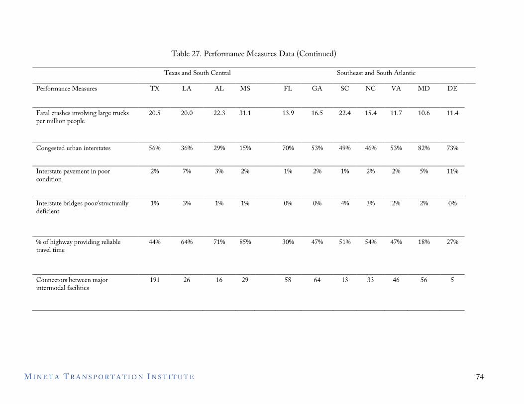
Table 27. Performance Measures Data (Continued)
Texas and South Central Southeast and South Atlantic
Performance Measures TX LA AL MS FL GA SC NC VA MD DE
Fatal crashes involving large trucks per million people
20.5 20.0 22.3 31.1 13.9 16.5 22.4 15.4 11.7 10.6 11.4
Congested urban interstates 56% 36% 29% 15% 70% 53% 49% 46% 53% 82% 73%
Interstate pavement in poor condition
2% 7% 3% 2% 1% 2% 1% 2% 2% 5% 11%
Interstate bridges poor/structurally deficient
1% 3% 1% 1% 0% 0% 4% 3% 2% 2% 0%
% of highway providing reliable travel time
44% 64% 71% 85% 30% 47% 51% 54% 47% 18% 27%
Connectors between major intermodal facilities
191 26 16 29 58 64 13 33 46 56 5
M I N E T A T R A N S P O R T A T I O N I N S T I T U T E 74
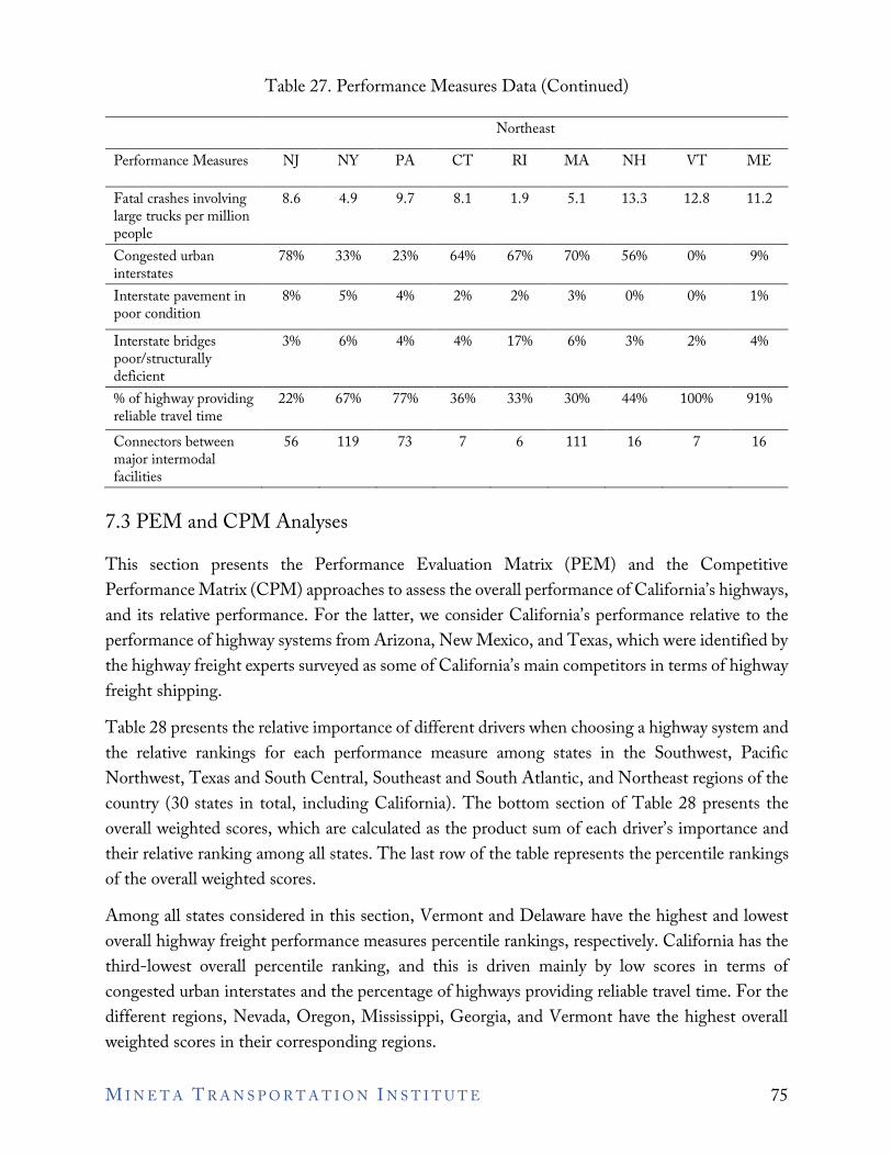
Table 27. Performance Measures Data (Continued)
Northeast Performance Measures NJ NY PA CT RI MA NH VT ME
Fatal crashes involving large trucks per million people
8.6 4.9 9.7 8.1 1.9 5.1 13.3 12.8 11.2
Congested urban interstates
78% 33% 23% 64% 67% 70% 56% 0% 9%
Interstate pavement in poor condition
8% 5% 4% 2% 2% 3% 0% 0% 1%
Interstate bridges poor/structurally deficient
3% 6% 4% 4% 17% 6% 3% 2% 4%
% of highway providing reliable travel time
22% 67% 77% 36% 33% 30% 44% 100% 91%
Connectors between 56 119 73 7 6 111 16 7 16 major intermodal facilities
7.3 PEM and CPM Analyses This section presents the Performance Evaluation Matrix (PEM) and the Competitive Performance Matrix (CPM) approaches to assess the overall performance of California’s highways, and its relative performance. For the latter, we consider California’s performance relative to the performance of highway systems from Arizona, New Mexico, and Texas, which were identified by the highway freight experts surveyed as some of California’s main competitors in terms of highway freight shipping. Table 28 presents the relative importance of different drivers when choosing a highway system and the relative rankings for each performance measure among states in the Southwest, Pacific Northwest, Texas and South Central, Southeast and South Atlantic, and Northeast regions of the country (30 states in total, including California). The bottom section of Table 28 presents the overall weighted scores, which are calculated as the product sum of each driver’s importance and their relative ranking among all states. The last row of the table represents the percentile rankings of the overall weighted scores. Among all states considered in this section, Vermont and Delaware have the highest and lowest overall highway freight performance measures percentile rankings, respectively. California has the third-lowest overall percentile ranking, and this is driven mainly by low scores in terms of congested urban interstates and the percentage of highways providing reliable travel time. For the different regions, Nevada, Oregon, Mississippi, Georgia, and Vermont have the highest overall weighted scores in their corresponding regions.
M I N E T A T R A N S P O R T A T I O N I N S T I T U T E 75
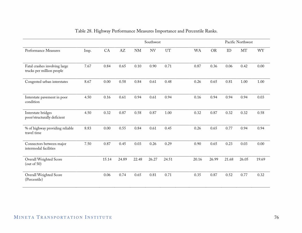
Table 28. Highway Performance Measures Importance and Percentile Ranks.
Southwest Pacific Northwest
Performance Measures Imp. CA AZ NM NV UT WA OR ID MT WY
Fatal crashes involving large trucks per million people
7.67 0.84 0.65 0.10 0.90 0.71 0.87 0.36 0.06 0.42 0.00
Congested urban interstates 8.67 0.00 0.58 0.84 0.61 0.48 0.26 0.65 0.81 1.00 1.00
Interstate pavement in poor condition
4.50 0.16 0.61 0.94 0.61 0.94 0.16 0.94 0.94 0.94 0.03
Interstate bridges poor/structurally deficient
4.50 0.32 0.87 0.58 0.87 1.00 0.32 0.87 0.32 0.32 0.58
% of highway providing reliable travel time
8.83 0.00 0.55 0.84 0.61 0.45 0.26 0.65 0.77 0.94 0.94
Connectors between major intermodal facilities
7.50 0.87 0.45 0.03 0.26 0.29 0.90 0.65 0.23 0.03 0.00
Overall Weighted Score (out of 50)
15.14 24.89 22.48 26.27 24.51 20.16 26.99 21.68 26.05 19.69
Overall Weighted Score (Percentile)
0.06 0.74 0.65 0.81 0.71 0.35 0.87 0.52 0.77 0.32
M I N E T A T R A N S P O R T A T I O N I N S T I T U T E 76
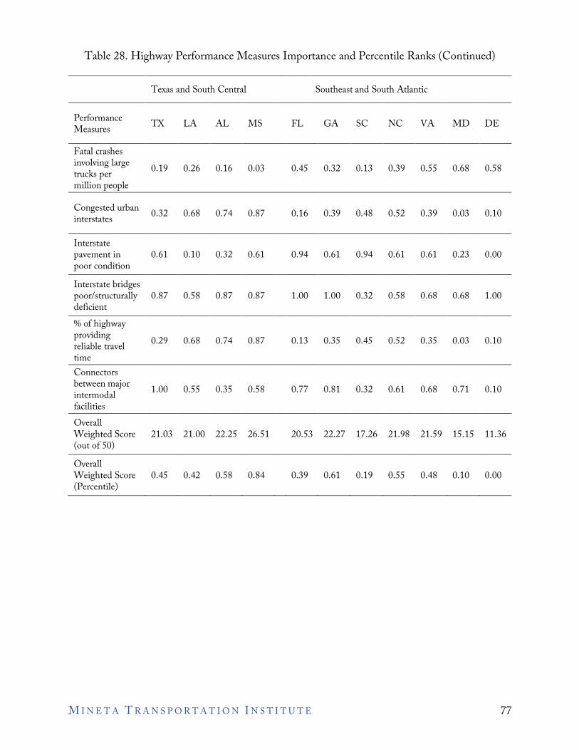
Table 28. Highway Performance Measures Importance and Percentile Ranks (Continued)
Texas and South Central Southeast and South Atlantic
Performance Measures TX LA AL MS FL GA SC NC VA MD DE
Fatal crashes involving large trucks per million people
0.19 0.26 0.16 0.03 0.45 0.32 0.13 0.39 0.55 0.68 0.58
Congested urban interstates 0.32 0.68 0.74 0.87 0.16 0.39 0.48 0.52 0.39 0.03 0.10
Interstate pavement in poor condition Interstate bridges poor/structurally deficient % of highway providing reliable travel time Connectors between major intermodal facilities Overall Weighted Score (out of 50) Overall Weighted Score (Percentile)
0.61
0.87
0.29
1.00
21.03
0.45
0.10
0.58
0.68
0.55
21.00
0.42
0.32
0.87
0.74
0.35
22.25
0.58
0.61
0.87
0.87
0.58
26.51
0.84
0.94
1.00
0.13
0.77
20.53
0.39
0.61
1.00
0.35
0.81
22.27
0.61
0.94
0.32
0.45
0.32
17.26
0.19
0.61
0.58
0.52
0.61
21.98
0.55
0.61
0.68
0.35
0.68
21.59
0.48
0.23
0.68
0.03
0.71
15.15
0.10
0.00
1.00
0.10
0.10
11.36
0.00
M I N E T A T R A N S P O R T A T I O N I N S T I T U T E 77
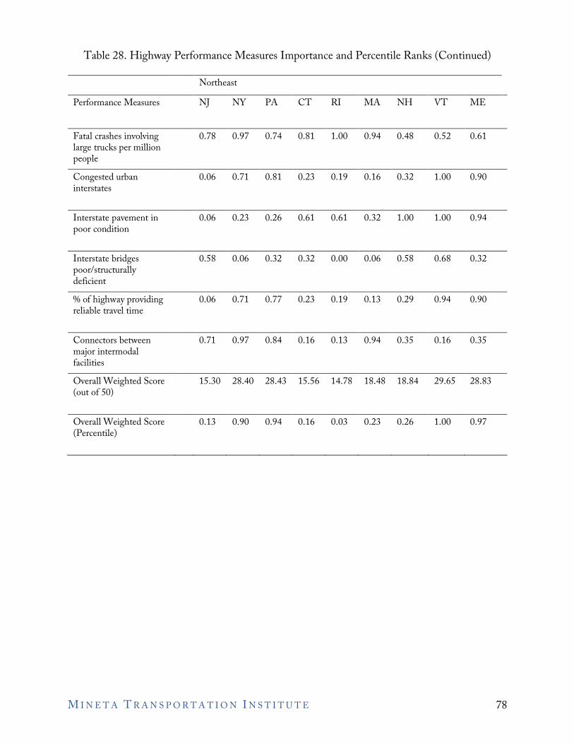
Table 28. Highway Performance Measures Importance and Percentile Ranks (Continued)
Northeast Performance Measures NJ NY PA CT RI MA NH VT ME
Fatal crashes involving large trucks per million people Congested urban interstates
0.78
0.06
0.97
0.71
0.74
0.81
0.81
0.23
1.00
0.19
0.94
0.16
0.48
0.32
0.52
1.00
0.61
0.90
Interstate pavement in poor condition
0.06 0.23 0.26 0.61 0.61 0.32 1.00 1.00 0.94
Interstate bridges poor/structurally deficient
0.58 0.06 0.32 0.32 0.00 0.06 0.58 0.68 0.32
% of highway providing reliable travel time
0.06 0.71 0.77 0.23 0.19 0.13 0.29 0.94 0.90
Connectors between major intermodal facilities
0.71 0.97 0.84 0.16 0.13 0.94 0.35 0.16 0.35
Overall Weighted Score (out of 50)
15.30 28.40 28.43 15.56 14.78 18.48 18.84 29.65 28.83
Overall Weighted Score (Percentile)
0.13 0.90 0.94 0.16 0.03 0.23 0.26 1.00 0.97
M I N E T A T R A N S P O R T A T I O N I N S T I T U T E 78
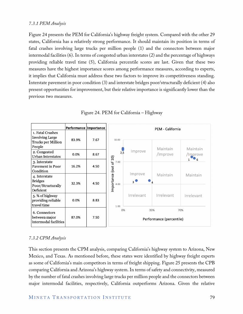
Importance PEM - California 1. Fatal Crashes Involving Large
83.9% 7.67 Trucks per Million People 2. Congested
0.0% 8.67 Urban Interstates 3. Interstate
woo J Maintain Maintain
2,, Improve /Improve /l~rove
0 1 .6 .-t
'+- 7.00 0
Pavement in Poor 16.2% 4.50 -::::, Condition 4. Interstate
..2. Improve QJ Maintain Maintain u
C:
Bridges 32.3% 4.50
Poor/Structurally 3. .4 ro -0 4.00
a. Deficient E
5. % of highway Irrelevant Irrelevant Irrelevant providing reliable 0.0% 8.83
travel time 1.00
6. Connectors 0% 35% 70%
between major 87.0% 7.50 intermodal facilities
Performance (percentile)
7.3.1 PEM Analysis
Figure 24 presents the PEM for California’s highway freight system. Compared with the other 29 states, California has a relatively strong performance. It should maintain its position in terms of fatal crashes involving large trucks per million people (1) and the connectors between major intermodal facilities (6). In terms of congested urban interstates (2) and the percentage of highways providing reliable travel time (5), California percentile scores are last. Given that these two measures have the highest importance scores among performance measures, according to experts, it implies that California must address these two factors to improve its competitiveness standing. Interstate pavement in poor condition (3) and interstate bridges poor/structurally deficient (4) also present opportunities for improvement, but their relative importance is significantly lower than the previous two measures.
Figure 24. PEM for California – Highway
7.3.2 CPM Analysis
This section presents the CPM analysis, comparing California’s highway system to Arizona, New Mexico, and Texas. As mentioned before, these states were identified by highway freight experts as some of California’s main competitors in terms of freight shipping. Figure 25 presents the CPB comparing California and Arizona’s highway system. In terms of safety and connectivity, measured by the number of fatal crashes involving large trucks per million people and the connectors between major intermodal facilities, respectively, California outperforms Arizona. Given the relative
M I N E T A T R A N S P O R T A T I O N I N S T I T U T E 79
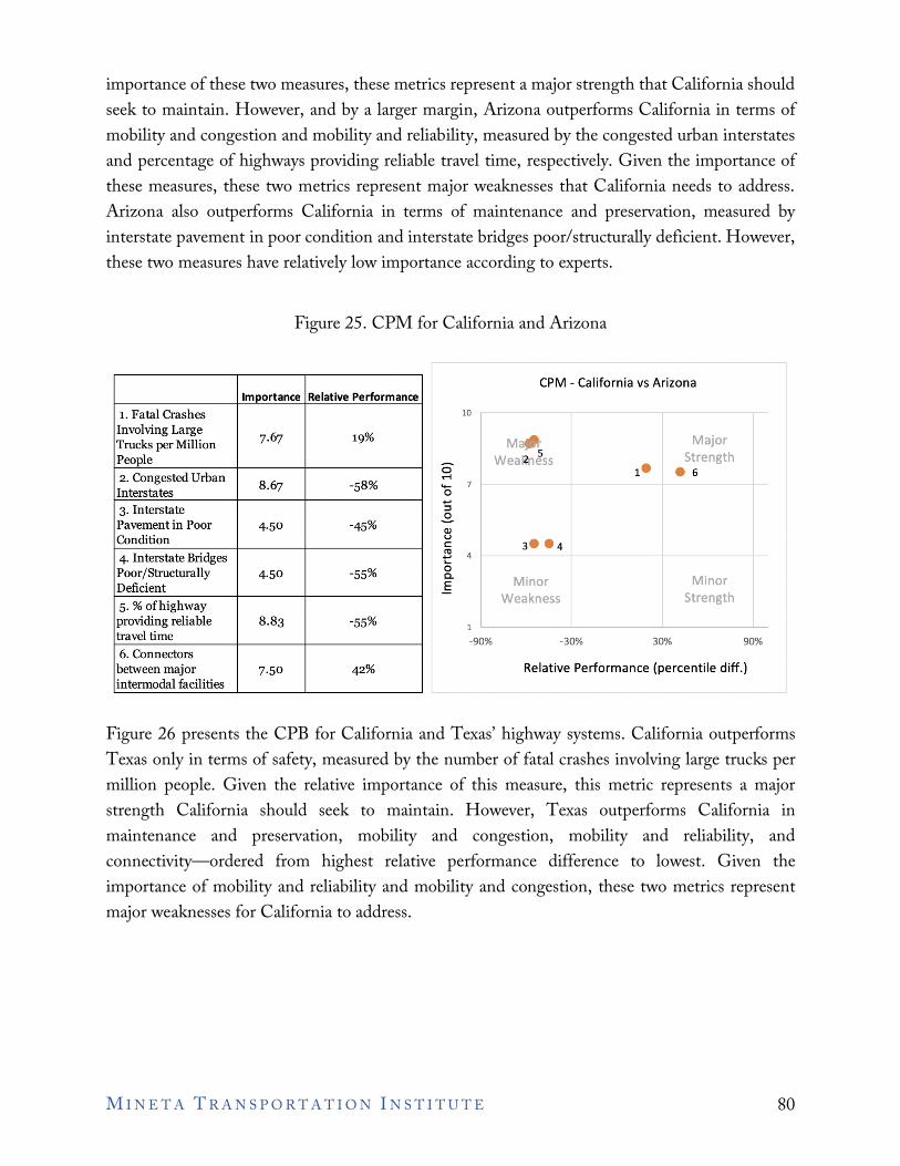
M I N E T A T R A N S P O R T A T I O N I N S T I T U T E 80
importance of these two measures, these metrics represent a major strength that California should seek to maintain. However, and by a larger margin, Arizona outperforms California in terms of mobility and congestion and mobility and reliability, measured by the congested urban interstates and percentage of highways providing reliable travel time, respectively. Given the importance of these measures, these two metrics represent major weaknesses that California needs to address. Arizona also outperforms California in terms of maintenance and preservation, measured by interstate pavement in poor condition and interstate bridges poor/structurally deficient. However, these two measures have relatively low importance according to experts.
Figure 25. CPM for California and Arizona
Figure 26 presents the CPB for California and Texas’ highway systems. California outperforms Texas only in terms of safety, measured by the number of fatal crashes involving large trucks per million people. Given the relative importance of this measure, this metric represents a major strength California should seek to maintain. However, Texas outperforms California in maintenance and preservation, mobility and congestion, mobility and reliability, and connectivity—ordered from highest relative performance difference to lowest. Given the importance of mobility and reliability and mobility and congestion, these two metrics represent major weaknesses for California to address.
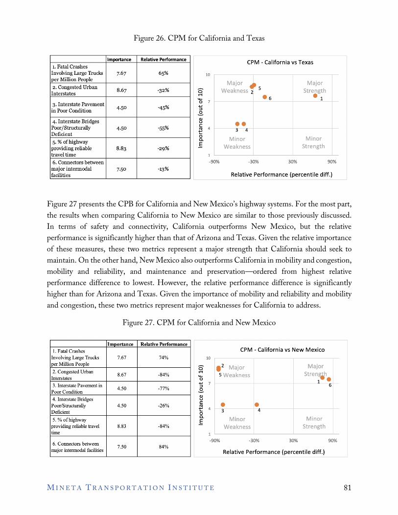
M I N E T A T R A N S P O R T A T I O N I N S T I T U T E 81
Figure 26. CPM for California and Texas
Figure 27 presents the CPB for California and New Mexico’s highway systems. For the most part, the results when comparing California to New Mexico are similar to those previously discussed. In terms of safety and connectivity, California outperforms New Mexico, but the relative performance is significantly higher than that of Arizona and Texas. Given the relative importance of these measures, these two metrics represent a major strength that California should seek to maintain. On the other hand, New Mexico also outperforms California in mobility and congestion, mobility and reliability, and maintenance and preservation—ordered from highest relative performance difference to lowest. However, the relative performance difference is significantly higher than for Arizona and Texas. Given the importance of mobility and reliability and mobility and congestion, these two metrics represent major weaknesses for California to address.
Figure 27. CPM for California and New Mexico
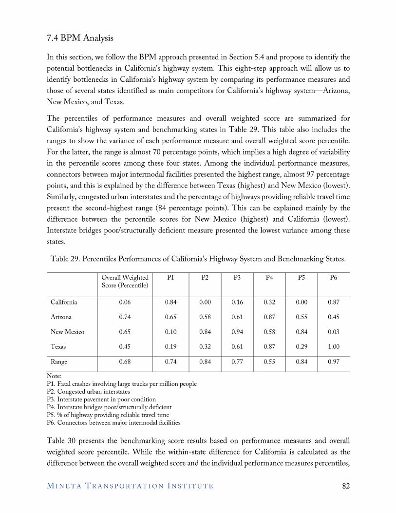
7.4 BPM Analysis In this section, we follow the BPM approach presented in Section 5.4 and propose to identify the potential bottlenecks in California’s highway system. This eight-step approach will allow us to identify bottlenecks in California’s highway system by comparing its performance measures and those of several states identified as main competitors for California’s highway system—Arizona, New Mexico, and Texas. The percentiles of performance measures and overall weighted score are summarized for California’s highway system and benchmarking states in Table 29. This table also includes the ranges to show the variance of each performance measure and overall weighted score percentile. For the latter, the range is almost 70 percentage points, which implies a high degree of variability in the percentile scores among these four states. Among the individual performance measures, connectors between major intermodal facilities presented the highest range, almost 97 percentage points, and this is explained by the difference between Texas (highest) and New Mexico (lowest). Similarly, congested urban interstates and the percentage of highways providing reliable travel time present the second-highest range (84 percentage points). This can be explained mainly by the difference between the percentile scores for New Mexico (highest) and California (lowest). Interstate bridges poor/structurally deficient measure presented the lowest variance among these states.
Table 29. Percentiles Performances of California’s Highway System and Benchmarking States.
Overall Weighted Score (Percentile)
P1 P2 P3 P4 P5 P6
California 0.06 0.84 0.00 0.16 0.32 0.00 0.87
Arizona 0.74 0.65 0.58 0.61 0.87 0.55 0.45
New Mexico 0.65 0.10 0.84 0.94 0.58 0.84 0.03
Texas 0.45 0.19 0.32 0.61 0.87 0.29 1.00
Range 0.68 0.74 0.84 0.77 0.55 0.84 0.97 Note: P1. Fatal crashes involving large trucks per million people P2. Congested urban interstates P3. Interstate pavement in poor condition P4. Interstate bridges poor/structurally deficient P5. % of highway providing reliable travel time P6. Connectors between major intermodal facilities
Table 30 presents the benchmarking score results based on performance measures and overall weighted score percentile. While the within-state difference for California is calculated as the difference between the overall weighted score and the individual performance measures percentiles,
M I N E T A T R A N S P O R T A T I O N I N S T I T U T E 82
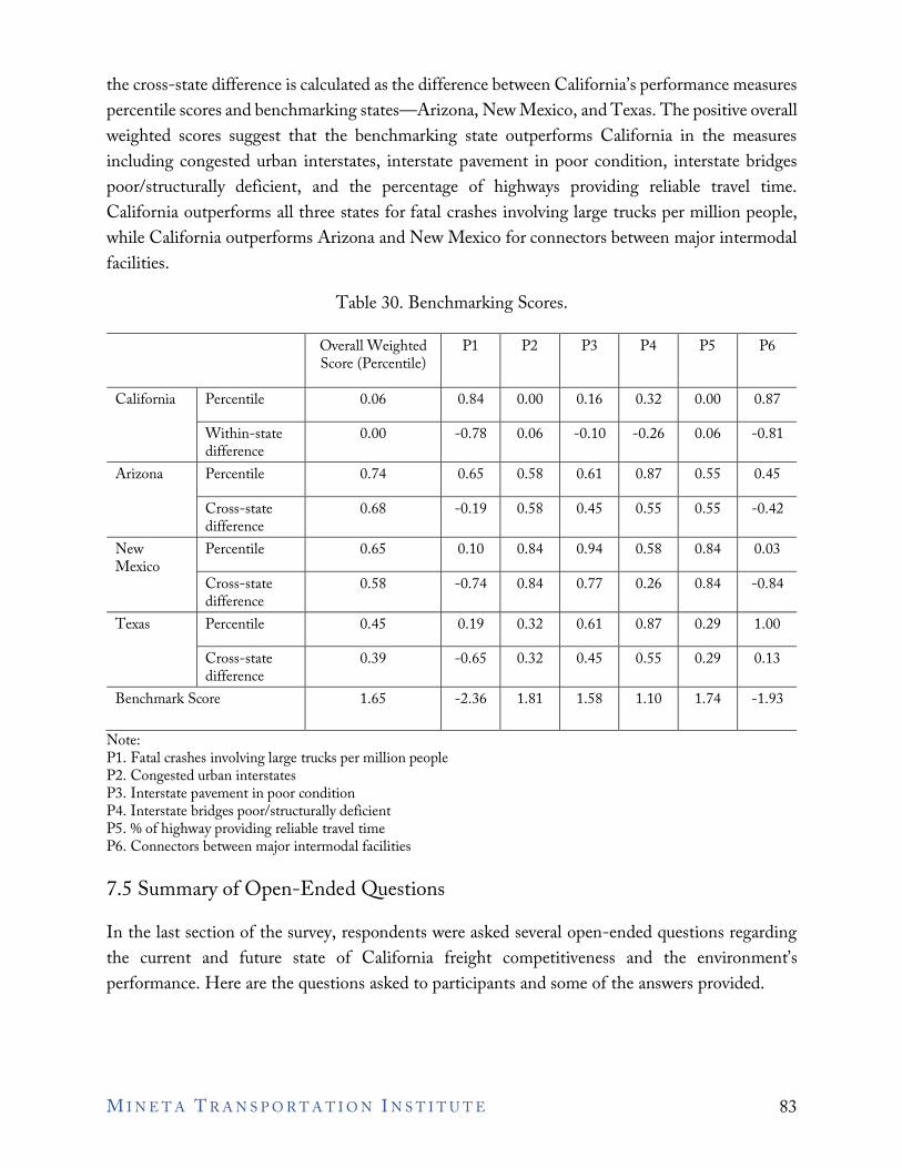
the cross-state difference is calculated as the difference between California’s performance measures percentile scores and benchmarking states—Arizona, New Mexico, and Texas. The positive overall weighted scores suggest that the benchmarking state outperforms California in the measures including congested urban interstates, interstate pavement in poor condition, interstate bridges poor/structurally deficient, and the percentage of highways providing reliable travel time. California outperforms all three states for fatal crashes involving large trucks per million people, while California outperforms Arizona and New Mexico for connectors between major intermodal facilities.
Table 30. Benchmarking Scores.
Overall Weighted Score (Percentile)
P1 P2 P3 P4 P5 P6
California Percentile 0.06 0.84 0.00 0.16 0.32 0.00 0.87
Within-state difference
0.00 -0.78 0.06 -0.10 -0.26 0.06 -0.81
Arizona Percentile 0.74 0.65 0.58 0.61 0.87 0.55 0.45
Cross-state difference
0.68 -0.19 0.58 0.45 0.55 0.55 -0.42
New Mexico
Percentile 0.65 0.10 0.84 0.94 0.58 0.84 0.03
Cross-state difference
0.58 -0.74 0.84 0.77 0.26 0.84 -0.84
Texas Percentile 0.45 0.19 0.32 0.61 0.87 0.29 1.00
Cross-state difference
0.39 -0.65 0.32 0.45 0.55 0.29 0.13
Benchmark Score 1.65 -2.36 1.81 1.58 1.10 1.74 -1.93
Note: P1. Fatal crashes involving large trucks per million people P2. Congested urban interstates P3. Interstate pavement in poor condition P4. Interstate bridges poor/structurally deficient P5. % of highway providing reliable travel time P6. Connectors between major intermodal facilities
7.5 Summary of Open-Ended Questions In the last section of the survey, respondents were asked several open-ended questions regarding the current and future state of California freight competitiveness and the environment’s performance. Here are the questions asked to participants and some of the answers provided.
M I N E T A T R A N S P O R T A T I O N I N S T I T U T E 83
7.5.1 Current state of California freight competitiveness
The section on the current state of California’s freight competitiveness asked respondents to identify California’s main competitors in terms of roadway shipping, major recent investment in infrastructure, and to identify some of the main bottlenecks in California’s highway system. Experts identified Arizona, New Mexico, and Texas as the country’s main competitor states to California, regarding roadway shipping. However, other states/areas were also mentioned, like Nevada, Georgia, South Carolina, Tennessee, Florida, the Tri-State area, Illinois, and Washington. In terms of recent infrastructure investments, experts cited $830 million spent to repair highways and bridges, improvements in highways (HOV lanes, more regular lanes, and toll roads), and the Gerald Desmond Bridge in Long Beach to assist traffic from the port. Specifics highway sections were also mentioned, like the sections of the 15-91, the 710, and the 60, to highlight recent infrastructure investments. In terms of bottlenecks, entire highway sections were mentioned as California’s key bottlenecks in the roadway freight system, like the 5, 10, 22, 91, 101, 405, and 605. Experts also cited most connections going through downtown Los Angeles and the Cajon pass, which involves sections of the 15-215 freeway. In addition, experts consider that the main connections between highways and other supply chain sectors is with seaports, and some consider this connection is the key to make California competitive.
7.5.2 The future of California freight competitiveness
Regarding the future of California’s freight competitiveness, respondents were also asked about how California’s highway system can become more competitive, the investments needed, and any potential future threats to California’s highway freight competitiveness. To become more competitive, experts cited the need for expanding highways and freight corridors, and providing incentives or subsidies to smaller/medium-sized distributors and independent owner/operators to compete better with large corporate farms and trucking companies.
In terms of investments to improve California’s highway competitiveness, experts cited investment for developing and expanding freight corridors and developing truck-specific routes to connect the ports with the main freight corridors in the country. Some experts also cited a better use of tax money and to provide training for dispatchers and drivers.
In terms of threats to California’s highway competitiveness, experts cited large corporations, like Amazon, and how they can create their own freight company and significantly curtail competition in the industry. Experts also cited excessive government regulations, like requiring zero-emission trucks, and continuing road deterioration.
M I N E T A T R A N S P O R T A T I O N I N S T I T U T E 84
7.6 Highway Performance with respect to the Environment, Sustainability, and Resilience
The last open-ended question section of the survey asked respondents about California’s highway system resilience, the environmental impact brought by the highway system, investments made and needed to be made to mitigate this environmental impact, and how the sustainability of California’s highway freight system might affect its competitiveness. For the most part, respondents felt that California’s freight system was resilient, and that air pollution was the main environmental impact brought by California freight system. In terms of investments needed to mitigate the environmental impacts, experts cited California’s zero emissions mandate, green freight trucks, and developing freight-exclusive lanes and corridors as ways to mitigate environmental impacts and increase California’s freight system competitiveness.
7.7 Conclusions 7.7.1 Findings
The findings from this section provide a clear picture of California’s competitiveness in highway freight relative to some of its main competitors. Given its relative percentile scores among 30 states, California should concentrate on implementing measures to reduce congestion for highway freight and invest in the maintenance and repair of highway pavement and bridges. Finding the financial resources to allocate to these projects could be a major challenge for California’s government. However, the importance and potential rewards from these investments make them a vital component of California’s highway freight competitive strategy.
7.7.2 Suggestions
While freight experts, for the most part, consider California’s relative competitiveness performance in highway freight as unsatisfactory, they might consider its performance can be significantly improved by addressing some basic infrastructure and regulatory issues. Experts frequently cited developing and enhancing freight-dedicated lanes to reduce highway congestion and improve reliable travel time. However, funding such projects might prove to be a prohibitive impediment given the current state of the economy. On the other hand, experts also considered that the state’s environmental regulations imposed on the industry might be too costly, too ambitious, and in some cases even unfeasible given the current technologies, like the regulations calling for zero-emission freight trucks. The main concern here is that those regulations might leave California in an even more disadvantaged position than its main competitors. Thus, the suggestion here might be for regulators to acknowledge California's current overall relative competitive performance, consider individual key drivers' relative performance, and work together with the industry to become more efficient and competitive and improve its relative standing in the industry.
M I N E T A T R A N S P O R T A T I O N I N S T I T U T E 85
7.7.3 Workforce Development Plan
Given federal and state goals to modernize thousands of miles of highways, roads, and bridges, that provide critical linkages to our communities, we will need a skilled and trained workforce and a pipeline of future employees. Preparing for this will involve union and non-union construction partnerships that include employers who promote and support the need for, and access to training. A suitable workforce pipeline development tool will be apprenticeship programs that focus not only on manual and machine operations, but also driver safety and awareness of regulations inter-and intra-statewide. Further, as we modernize our infrastructure, we will develop more zero and near zero technologies, as a result, maintenance workers accustomed to working on diesel engine trucks and building equipment will need to acquire skills necessary for working with new technologies that will power the vehicles of the future. Employers and government officials need to understand and promote the value of retraining and outreach to build a pipeline of younger, tech-savvy workers who are comfortable with new learning tools such as virtual reality and artificial intelligence. These lend efficiency and ultimately cost reduction with less accidents and turnover.
M I N E T A T R A N S P O R T A T I O N I N S T I T U T E 86
8. Freight Rails 8.1 Introduction The U.S. freight rail network contains close to 140,000 route miles in length and supports a nearly $80 billion industry with 167,000 jobs across seven Class I railroads (those with annual operating revenues larger than $490 million), 22 Class II/regional railroads, and 582 Class III/short line railroads (US Department of Transportation 2021). California’s 5,295-mile freight rail network is a small proportion of the U.S. network; however, it handled $159.6 million tons of commodities in 2013, and ranked eighth among states by rail tons originated in 2012. The state is served by two Class I railroads (see Figure 28), BNSF and Union Pacific, and 27 Class III short lines.
M I N E T A T R A N S P O R T A T I O N I N S T I T U T E 87
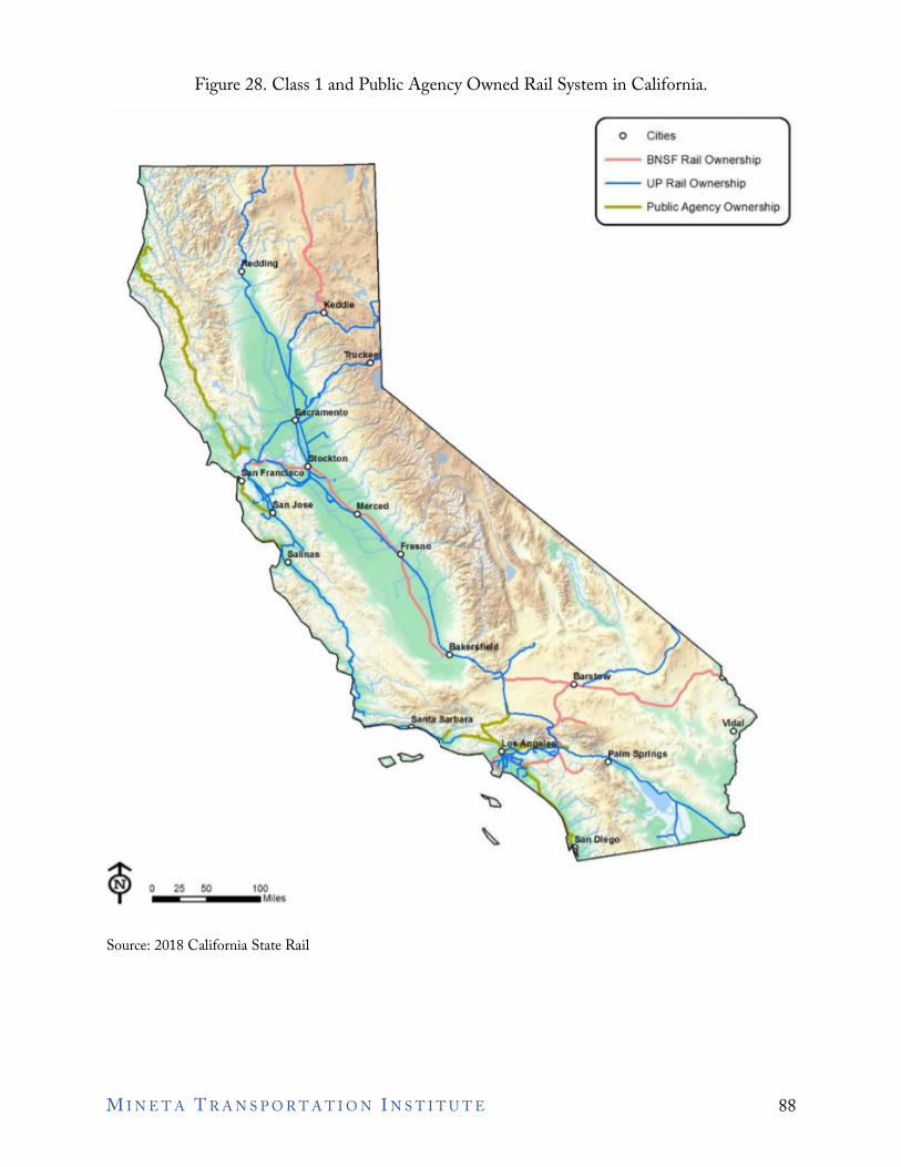
C.bes
BNSF Rad Ownenh1p
- UP Ra,t Ownership
- Public Agen:y OwnerSh1p
0 25 50 100 11111,.;;;i:::::::::,i ___ M,les
o
Figure 28. Class 1 and Public Agency Owned Rail System in California.
Source: 2018 California State Rail
M I N E T A T R A N S P O R T A T I O N I N S T I T U T E 88
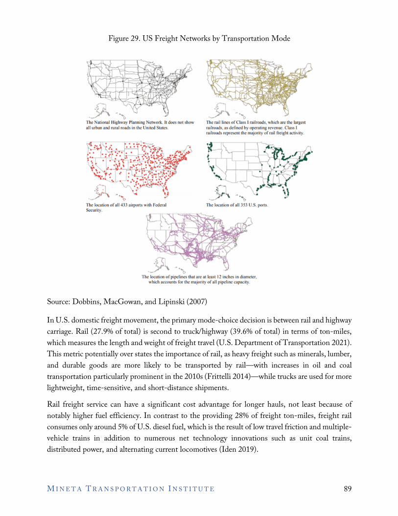
·'"o The National Highway Planning Network. h does not show all urban .tnd rural roods in the United S1ates.
♦• ♦ :►.: •• • .. ~ .,.,,,,. ♦> • • .... ♦'
: : r •, ~•-,.,_-.,.,,..,
••. J :. ·f 9
-~~. ·~~ --\ The locntion of nll 433 airports with Fc<lcrnl Security.
.. "''"<>
.. ·'"o The rail lines of Closs I rail roods, which arc the largest railroads, a.s defined by operating revenue. Class I milro3ds represent the majori1y of mil freight a.ctivi1y.
~-i \ .... __
-~7 -~ ,_;:;r'\ () The locntion of nll 353 U.S. ports.
The locauon of pipelines that arc at least 12 mchcs m diameter. which accounts for the majority of all pipeline cap.,.city.
Figure 29. US Freight Networks by Transportation Mode
Source: Dobbins, MacGowan, and Lipinski (2007)
In U.S. domestic freight movement, the primary mode-choice decision is between rail and highway carriage. Rail (27.9% of total) is second to truck/highway (39.6% of total) in terms of ton-miles, which measures the length and weight of freight travel (U.S. Department of Transportation 2021). This metric potentially over states the importance of rail, as heavy freight such as minerals, lumber, and durable goods are more likely to be transported by rail—with increases in oil and coal transportation particularly prominent in the 2010s (Frittelli 2014)—while trucks are used for more lightweight, time-sensitive, and short-distance shipments. Rail freight service can have a significant cost advantage for longer hauls, not least because of notably higher fuel efficiency. In contrast to the providing 28% of freight ton-miles, freight rail consumes only around 5% of U.S. diesel fuel, which is the result of low travel friction and multiple-vehicle trains in addition to numerous net technology innovations such as unit coal trains, distributed power, and alternating current locomotives (Iden 2019).
M I N E T A T R A N S P O R T A T I O N I N S T I T U T E 89
� � � �
8.2 Literature review Little prior research explicitly explores the competitiveness of U.S. freight rail. Some literature explores freight rail competitiveness in Europe (Crozet 2017; Dedík, Ga parík, Záhumenská,
Upták, and H ebí ek 2018), Australia (Ghaderi, Cahoon, and Nguyen 2017; Ghaderi, Fei, and Cahoon 2015), and Africa (Saruchera 2017), we focus on studies of the U.S. industry. Some literature uses mathematical or computational modeling to explore engineering, planning, or network questions, such as operations planning (Barbour, Mori, Kuppa, and Work 2018; Crevier, Cordeau, and Savard 2012; Woodburn 2019), network design (Dolinayova, L’Och, and Kanis 2015; Uddin and Huynh 2015; Yaghni and Akhavan 2012), and emissions modeling (Aditjandra, Zunder, Islam, and Palacin 2016; Janic and Vleugel 2012; Kirschstein and Meisel 2015; Li and Zhang 2020). While these studies provide some implicit insight into the competitiveness of California’s rail freight system, they are beyond the scope of our study. More relevant to this study are the broader productivity improvement trends since the deregulation of the freight rail industry through the Staggers Act of 1980 (Kriem 2011). During this period, Class I railroads halved the real costs per ton-mile despite higher than inflation increases in fuel costs, with the greatest productivity improvements seen in high-volume and long-distance shipments (Martland 2012). The Staggers Act has shaped the sector and contributed to productivity and pricing improvements (Bitzan and Keeler 2014). However, Martland (2012) argues compellingly that other factors such as technological innovations, labor agreements, improved management, and policy responses to the Northeast Rail Crisis played a greater role in productivity improvements. Despite such productivity improvements, rail’s cost and efficiency advantage is often eroded by pickup and delivery expenses, route circuitry, and actual equipment utilization. As such, U.S. railroads carry a very small share of intermediate and finished products (Boyer 2014). Since not all destinations are served by rail, there can be additional handling and trucking delivery costs. While Figure 29 suggests that Class I railroads have a large coverage, especially in the Eastern U.S., the road network is far more localized and extensive in coverage. Other logistical expenses may increase due to factors such as the large size of rail deliveries, slow transit times, and reliability issues (O'Rourke et al. 2015). One possible reason for the limited number of studies on U.S. freight rail competitiveness is the lack of publicly available industry data (Interview with Nicholas Little; Interview with Don Norton). Rail performance metrics were previously collated on the independent website “railroadpm.org”, which reported weekly Class I figures for terminal dwell, average train speed,
M I N E T A T R A N S P O R T A T I O N I N S T I T U T E 90
and cars online.2 Figures for terminal dwell, average train speed, and cars online are now available from the different company websites (see Table 31), as well as the U.S. Surface Transportation Board website;3 however, there are inconsistencies between the data provided. One issue is that only terminal dwell data are provided by location for all trains; other metrics are not available across our locations of interest (see Table 32). Data are provided by regions for cars online, but only for Grains and Coal, which account for approximately 30% of Union Pacific carloads and 45% of BNSF carloads. In addition, the available carloads data are not particularly illuminating. Moreover, not all companies provide these data by location. This study uses the above data, alongside state-level data from 2017 provided by Association of American Railroads. Given the limited number of studies of freight rail competitiveness, and the limited publicly available data, there is significant scope for contribution to the literature from our study. This study combines data gathered from structured interviews of freight rail experts with publicly available freight rail data by location. Using the CPM, PEM, and BPM approaches outlined in prior sections allows us to identify the strengths, weaknesses, bottlenecks, and areas of improvement for different regions, especially with respect to California. Moreover, these approaches allow us to compare freight rail’s performance with other transportation sectors, as outlined later in the report. In addition, detailed interviews with industry experts revealed potential policy changes, infrastructure investments, workforce needs, and bottleneck improvements that can improve California’s freight rail competitiveness.
2 “This Railroad Performance Measures website was created in 1999 to allow the major North American railroads to report performance data to their customers. Over the years, the railroads have expanded the amount of service-related information that they publish on their own websites and via email and social media—including performance data such as the three service measures that were reported on this site, customer service alerts, network service advisories, etc.—limiting the need for this website.” https://railroadpm.org/ 3https://www.stb.gov/stb/railserviceissues/rail_service_reports.html#loaded
M I N E T A T R A N S P O R T A T I O N I N S T I T U T E 91
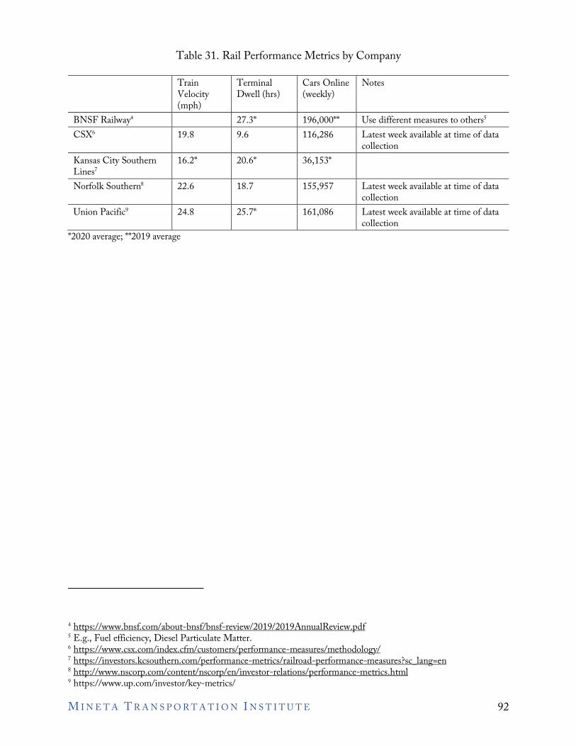
Table 31. Rail Performance Metrics by Company
Train Velocity (mph)
Terminal Dwell (hrs)
Cars Online (weekly)
Notes
BNSF Railway4 27.3* 196,000** Use different measures to others5
CSX6 19.8 9.6 116,286 Latest week available at time of data collection
Kansas City Southern Lines7
16.2* 20.6* 36,153*
Norfolk Southern8 22.6 18.7 155,957 Latest week available at time of data collection
Union Pacific9 24.8 25.7* 161,086 Latest week available at time of data collection
*2020 average; **2019 average
4 https://www.bnsf.com/about-bnsf/bnsf-review/2019/2019AnnualReview.pdf 5 E.g., Fuel efficiency, Diesel Particulate Matter. 6 https://www.csx.com/index.cfm/customers/performance-measures/methodology/ 7 https://investors.kcsouthern.com/performance-metrics/railroad-performance-measures?sc_lang=en 8 http://www.nscorp.com/content/nscorp/en/investor-relations/performance-metrics.html 9 https://www.up.com/investor/key-metrics/
M I N E T A T R A N S P O R T A T I O N I N S T I T U T E 92
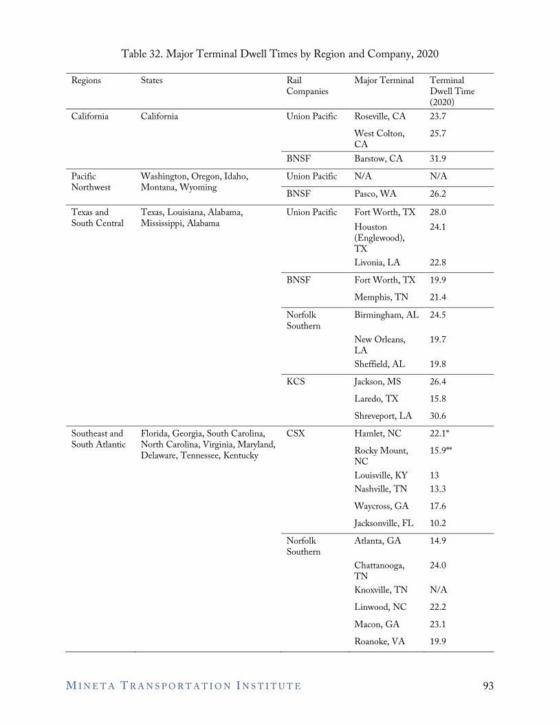
Table 32. Major Terminal Dwell Times by Region and Company, 2020
Regions States Rail Companies
Major Terminal Terminal Dwell Time (2020)
California California Union Pacific Roseville, CA 23.7 West Colton, CA
25.7
BNSF Barstow, CA 31.9 Pacific Northwest
Washington, Oregon, Idaho, Montana, Wyoming
Union Pacific BNSF
N/A Pasco, WA
N/A 26.2
Texas and South Central
Texas, Louisiana, Alabama, Mississippi, Alabama
Union Pacific Fort Worth, TX Houston (Englewood), TX
28.0 24.1
Livonia, LA 22.8 BNSF Fort Worth, TX 19.9
Memphis, TN 21.4 Norfolk Southern
Birmingham, AL 24.5
New Orleans, LA
19.7
Sheffield, AL 19.8 KCS Jackson, MS 26.4
Laredo, TX 15.8 Shreveport, LA 30.6
Southeast and Florida, Georgia, South Carolina, CSX Hamlet, NC 22.1* South Atlantic North Carolina, Virginia, Maryland, Rocky Mount, 15.9** Delaware, Tennessee, Kentucky NC
Louisville, KY 13 Nashville, TN 13.3 Waycross, GA 17.6 Jacksonville, FL 10.2
Norfolk Atlanta, GA 14.9 Southern
Chattanooga, 24.0 TN Knoxville, TN N/A Linwood, NC 22.2 Macon, GA 23.1 Roanoke, VA 19.9
M I N E T A T R A N S P O R T A T I O N I N S T I T U T E 93
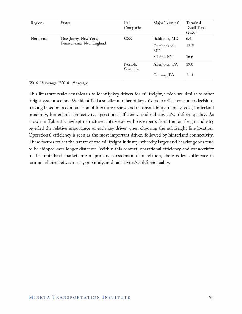
Regions States Rail Companies
Major Terminal Terminal Dwell Time (2020)
Northeast New Jersey, New York, Pennsylvania, New England
CSX Baltimore, MD Cumberland, MD
6.4 12.2*
Selkirk, NY 16.6 Norfolk Southern
Allentown, PA 19.0
Conway, PA 21.4 *2016–18 average; **2018–19 average
This literature review enables us to identify key drivers for rail freight, which are similar to other freight system sectors. We identified a smaller number of key drivers to reflect consumer decision-making based on a combination of literature review and data availability, namely: cost, hinterland proximity, hinterland connectivity, operational efficiency, and rail service/workforce quality. As shown in Table 33, in-depth structured interviews with six experts from the rail freight industry revealed the relative importance of each key driver when choosing the rail freight line location. Operational efficiency is seen as the most important driver, followed by hinterland connectivity. These factors reflect the nature of the rail freight industry, whereby larger and heavier goods tend to be shipped over longer distances. Within this context, operational efficiency and connectivity to the hinterland markets are of primary consideration. In relation, there is less difference in location choice between cost, proximity, and rail service/workforce quality.
M I N E T A T R A N S P O R T A T I O N I N S T I T U T E 94
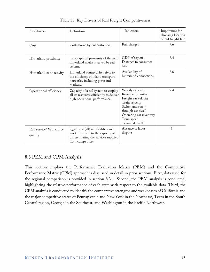
Table 33. Key Drivers of Rail Freight Competitiveness
Key drivers Definition Indicators Importance for choosing location of rail freight line
Cost Costs borne by rail customers Rail charges 7.6
Hinterland proximity Geographical proximity of the main hinterland markets served by rail system.
GDP of region Distance to consumer base
7.4
Hinterland connectivity Hinterland connectivity refers to the efficiency of inland transport networks, including ports and roadway.
Availability of hinterland connections
8.6
Operational efficiency Capacity of a rail system to employ all its resources efficiently to deliver high operational performance.
Weekly carloads Revenue ton miles Freight car velocity Train velocity Switch and run— through car dwell Operating car inventory Train speed Terminal dwell
9.4
Rail service/ Workforce quality
Quality of (all) rail facilities and workforce, and to the capacity of differentiating the services supplied from competitors.
Absence of labor dispute
7
8.3 PEM and CPM Analysis This section employs the Performance Evaluation Matrix (PEM) and the Competitive Performance Matrix (CPM) approaches discussed in detail in prior sections. First, data used for the regional comparison is provided in section 8.3.1. Second, the PEM analysis is conducted, highlighting the relative performance of each state with respect to the available data. Third, the CPM analysis is conducted to identify the comparative strengths and weaknesses of California and the major competitive states of Pennsylvania and New York in the Northeast, Texas in the South Central region, Georgia in the Southeast, and Washington in the Pacific Northwest.
M I N E T A T R A N S P O R T A T I O N I N S T I T U T E 95
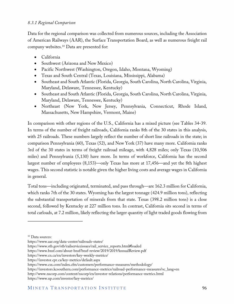
8.3.1 Regional Comparison
Data for the regional comparison was collected from numerous sources, including the Association of American Railways (AAR), the Surface Transportation Board, as well as numerous freight rail company websites.10 Data are presented for:
• California • Southwest (Arizona and New Mexico) • Pacific Northwest (Washington, Oregon, Idaho, Montana, Wyoming) • Texas and South Central (Texas, Louisiana, Mississippi, Alabama) • Southeast and South Atlantic (Florida, Georgia, South Carolina, North Carolina, Virginia,
Maryland, Delaware, Tennessee, Kentucky) • Southeast and South Atlantic (Florida, Georgia, South Carolina, North Carolina, Virginia,
Maryland, Delaware, Tennessee, Kentucky) • Northeast (New York, New Jersey, Pennsylvania, Connecticut, Rhode Island,
Massachusetts, New Hampshire, Vermont, Maine)
In comparison with other regions of the U.S., California has a mixed picture (see Tables 34-39. In terms of the number of freight railroads, California ranks 8th of the 30 states in this analysis, with 25 railroads. These numbers largely reflect the number of short line railroads in the state; in comparison Pennsylvania (60), Texas (52), and New York (37) have many more. California ranks 3rd of the 30 states in terms of freight railroad mileage, with 4,828 miles; only Texas (10,506 miles) and Pennsylvania (5,130) have more. In terms of workforce, California has the second largest number of employees (8,153)—only Texas has more at 17,456—and yet the 8th highest wages. This second statistic is notable given the higher living costs and average wages in California in general. Total tons—including originated, terminated, and pass through—are 162.3 million for California, which ranks 7th of the 30 states. Wyoming has the largest tonnage (424.9 million tons), reflecting the substantial transportation of minerals from that state. Texas (398.2 million tons) is a close second, followed by Kentucky at 227 million tons. In contrast, California sits second in terms of total carloads, at 7.2 million, likely reflecting the larger quantity of light traded goods flowing from
10 Data sources: https://www.aar.org/data-center/railroads-states/ https://www.stb.gov/stb/railserviceissues/rail_service_reports.html#loaded https://www.bnsf.com/about-bnsf/bnsf-review/2019/2019AnnualReview.pdf https://www.cn.ca/en/investors/key-weekly-metrics/ https://investor.cpr.ca/key-metrics/default.aspx https://www.csx.com/index.cfm/customers/performance-measures/methodology/ https://investors.kcsouthern.com/performance-metrics/railroad-performance-measures?sc_lang=en http://www.nscorp.com/content/nscorp/en/investor-relations/performance-metrics.html https://www.up.com/investor/key-metrics/
M I N E T A T R A N S P O R T A T I O N I N S T I T U T E 96
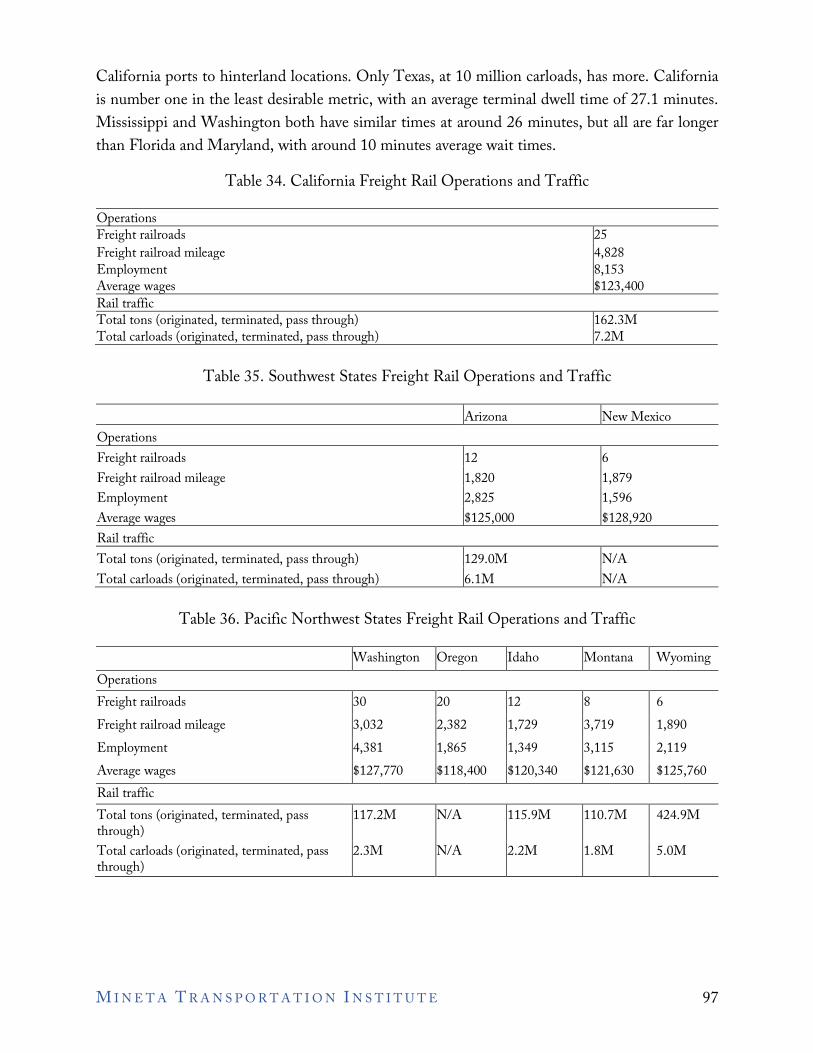
I I I I
California ports to hinterland locations. Only Texas, at 10 million carloads, has more. California is number one in the least desirable metric, with an average terminal dwell time of 27.1 minutes. Mississippi and Washington both have similar times at around 26 minutes, but all are far longer than Florida and Maryland, with around 10 minutes average wait times.
Table 34. California Freight Rail Operations and Traffic
Operations Freight railroads 25 Freight railroad mileage 4,828 Employment 8,153 Average wages $123,400 Rail traffic Total tons (originated, terminated, pass through) Total carloads (originated, terminated, pass through)
162.3M 7.2M
Table 35. Southwest States Freight Rail Operations and Traffic
Arizona New Mexico Operations Freight railroads 12 6 Freight railroad mileage 1,820 1,879 Employment 2,825 1,596 Average wages $125,000 $128,920 Rail traffic Total tons (originated, terminated, pass through) 129.0M N/A Total carloads (originated, terminated, pass through) 6.1M N/A
Table 36. Pacific Northwest States Freight Rail Operations and Traffic
Washington Oregon Idaho Montana Wyoming Operations Freight railroads Freight railroad mileage Employment Average wages
30 3,032 4,381 $127,770
20 2,382 1,865 $118,400
12 1,729 1,349 $120,340
8 3,719 3,115 $121,630
6 1,890 2,119 $125,760
Rail traffic Total tons (originated, terminated, pass through) Total carloads (originated, terminated, pass through)
117.2M
2.3M
N/A
N/A
115.9M
2.2M
110.7M
1.8M
424.9M
5.0M
M I N E T A T R A N S P O R T A T I O N I N S T I T U T E 97
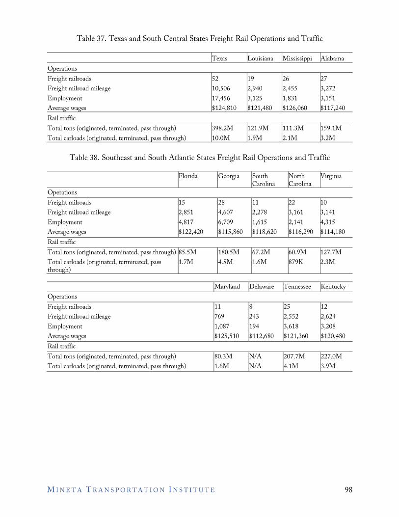
I I I I
I I I I
I I I I
I I I I
Table 37. Texas and South Central States Freight Rail Operations and Traffic
Texas Louisiana Mississippi Alabama Operations Freight railroads Freight railroad mileage Employment Average wages
52 10,506 17,456 $124,810
19 2,940 3,125 $121,480
26 2,455 1,831 $126,060
27 3,272 3,151 $117,240
Rail traffic Total tons (originated, terminated, pass through) Total carloads (originated, terminated, pass through)
398.2M 10.0M
121.9M 1.9M
111.3M 2.1M
159.1M 3.2M
Table 38. Southeast and South Atlantic States Freight Rail Operations and Traffic
Florida Georgia South Carolina
North Carolina
Virginia
Operations Freight railroads Freight railroad mileage Employment Average wages
15 2,851 4,817 $122,420
28 4,607 6,709 $115,860
11 2,278 1,615 $118,620
22 3,161 2,141 $116,290
10 3,141 4,315 $114,180
Rail traffic Total tons (originated, terminated, pass through) Total carloads (originated, terminated, pass through)
85.5M 1.7M
180.5M 4.5M
67.2M 1.6M
60.9M 879K
127.7M 2.3M
Maryland Delaware Tennessee Kentucky Operations Freight railroads Freight railroad mileage Employment Average wages
11 769 1,087 $125,510
8 243 194 $112,680
25 2,552 3,618 $121,360
12 2,624 3,208 $120,480
Rail traffic Total tons (originated, terminated, pass through) Total carloads (originated, terminated, pass through)
80.3M 1.6M
N/A N/A
207.7M 4.1M
227.0M 3.9M
M I N E T A T R A N S P O R T A T I O N I N S T I T U T E 98
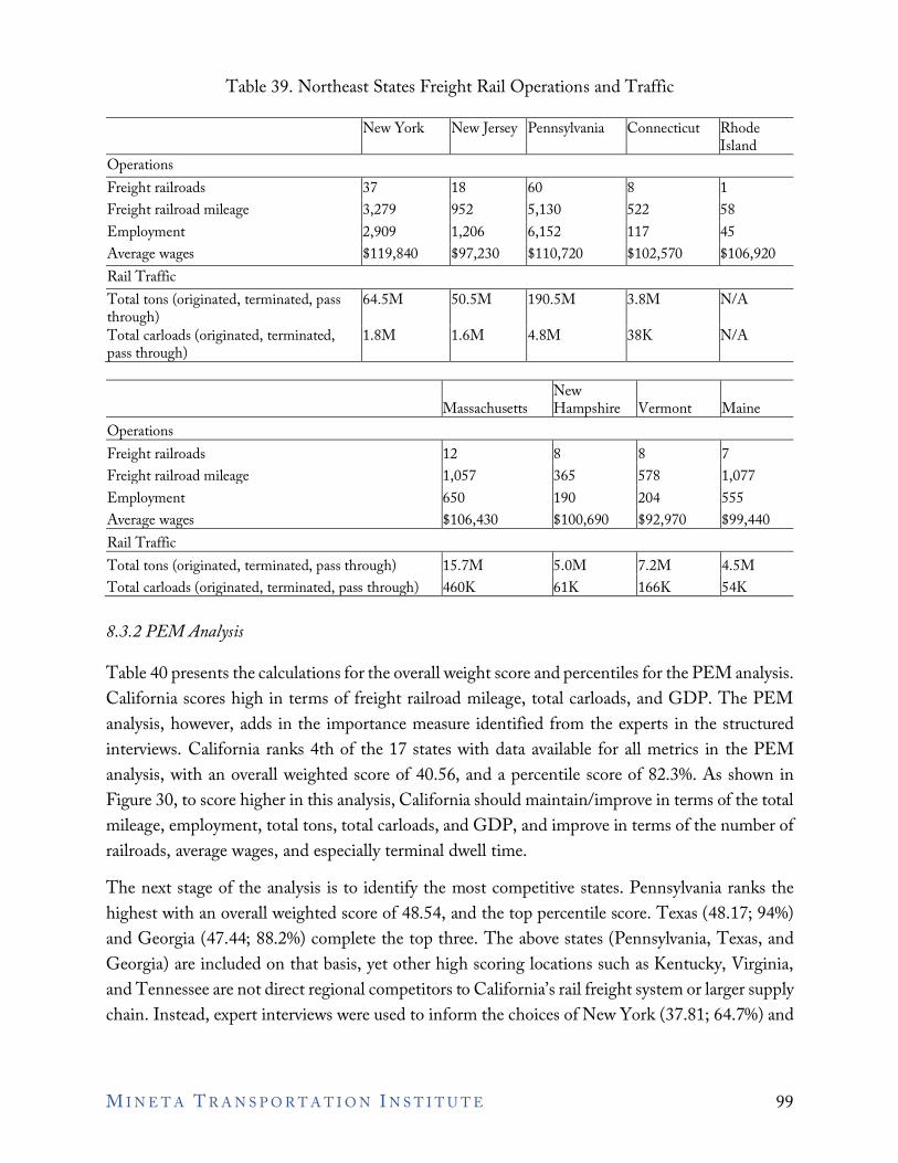
I I I I I
I I I I I
I I I I
Table 39. Northeast States Freight Rail Operations and Traffic
New York New Jersey Pennsylvania Connecticut Rhode Island
Operations Freight railroads Freight railroad mileage Employment Average wages
37 3,279 2,909 $119,840
18 952 1,206 $97,230
60 5,130 6,152 $110,720
8 522 117 $102,570
1 58 45 $106,920
Rail Traffic Total tons (originated, terminated, pass through) Total carloads (originated, terminated, pass through)
64.5M
1.8M
50.5M
1.6M
190.5M
4.8M
3.8M
38K
N/A
N/A
Massachusetts New Hampshire Vermont Maine
Operations Freight railroads Freight railroad mileage Employment Average wages
12 1,057 650 $106,430
8 365 190 $100,690
8 578 204 $92,970
7 1,077 555 $99,440
Rail Traffic Total tons (originated, terminated, pass through) Total carloads (originated, terminated, pass through)
15.7M 460K
5.0M 61K
7.2M 166K
4.5M 54K
8.3.2 PEM Analysis
Table 40 presents the calculations for the overall weight score and percentiles for the PEM analysis. California scores high in terms of freight railroad mileage, total carloads, and GDP. The PEM analysis, however, adds in the importance measure identified from the experts in the structured interviews. California ranks 4th of the 17 states with data available for all metrics in the PEM analysis, with an overall weighted score of 40.56, and a percentile score of 82.3%. As shown in Figure 30, to score higher in this analysis, California should maintain/improve in terms of the total mileage, employment, total tons, total carloads, and GDP, and improve in terms of the number of railroads, average wages, and especially terminal dwell time. The next stage of the analysis is to identify the most competitive states. Pennsylvania ranks the highest with an overall weighted score of 48.54, and the top percentile score. Texas (48.17; 94%) and Georgia (47.44; 88.2%) complete the top three. The above states (Pennsylvania, Texas, and Georgia) are included on that basis, yet other high scoring locations such as Kentucky, Virginia, and Tennessee are not direct regional competitors to California’s rail freight system or larger supply chain. Instead, expert interviews were used to inform the choices of New York (37.81; 64.7%) and
M I N E T A T R A N S P O R T A T I O N I N S T I T U T E 99
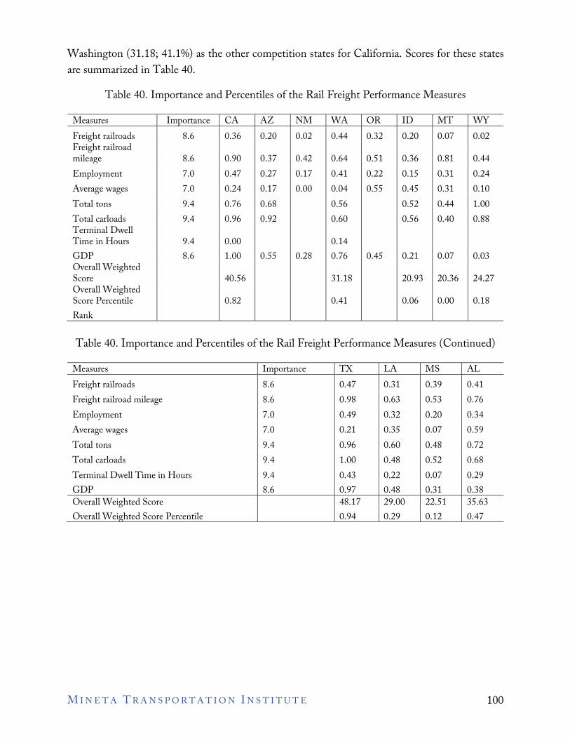
Washington (31.18; 41.1%) as the other competition states for California. Scores for these states are summarized in Table 40.
Table 40. Importance and Percentiles of the Rail Freight Performance Measures
Measures Importance CA AZ NM WA OR ID MT WY Freight railroads Freight railroad
8.6 0.36 0.20 0.02 0.44 0.32 0.20 0.07 0.02
mileage 8.6 0.90 0.37 0.42 0.64 0.51 0.36 0.81 0.44 Employment 7.0 0.47 0.27 0.17 0.41 0.22 0.15 0.31 0.24 Average wages 7.0 0.24 0.17 0.00 0.04 0.55 0.45 0.31 0.10 Total tons 9.4 0.76 0.68 0.56 0.52 0.44 1.00 Total carloads Terminal Dwell
9.4 0.96 0.92 0.60 0.56 0.40 0.88
Time in Hours 9.4 0.00 0.14 GDP Overall Weighted
8.6 1.00 0.55 0.28 0.76 0.45 0.21 0.07 0.03
Score Overall Weighted
40.56 31.18 20.93 20.36 24.27
Score Percentile Rank
0.82 0.41 0.06 0.00 0.18
Table 40. Importance and Percentiles of the Rail Freight Performance Measures (Continued)
Measures Importance TX LA MS AL Freight railroads Freight railroad mileage Employment Average wages Total tons Total carloads Terminal Dwell Time in Hours GDP
8.6 8.6 7.0 7.0 9.4 9.4 9.4 8.6
0.47 0.98 0.49 0.21 0.96 1.00 0.43 0.97
0.31 0.63 0.32 0.35 0.60 0.48 0.22 0.48
0.39 0.53 0.20 0.07 0.48 0.52 0.07 0.31
0.41 0.76 0.34 0.59 0.72 0.68 0.29 0.38
Overall Weighted Score Overall Weighted Score Percentile
48.17 0.94
29.00 0.29
22.51 0.12
35.63 0.47
M I N E T A T R A N S P O R T A T I O N I N S T I T U T E 100
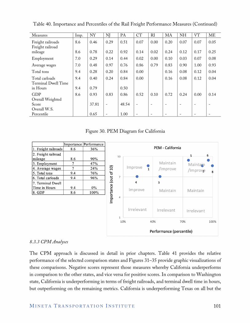
Performance 1. Freight railroads 8.6 36% PEM - California
2. Freight railroad mileage 8.6 90% 3. Employment 7 47% 4. Average wages 7 24% 5. Total tons 9.4 76%
10 5 6
Maintain • • 0 Improve • Maint • .-t 1 /Improve /lmpro '+- 8 0
6. Total carloads 9.4 96% .... 7 • • ~
7. Terminal Dwell .£. 4 3 Q)
Time in Hours 9.4 0% 8.GDP 8.6 100%
u C: Improve Maintain Maintain n, t 0 4 a. E
Irrelevant Irrelevant Irrelevant
1
10% 40% 70% 100%
Performance (percentile)
Table 40. Importance and Percentiles of the Rail Freight Performance Measures (Continued)
Measures Imp. NY NJ PA CT RI MA NH VT ME Freight railroads Freight railroad
8.6 0.46 0.29 0.51 0.07 0.00 0.20 0.07 0.07 0.05
mileage 8.6 0.78 0.22 0.92 0.14 0.02 0.24 0.12 0.17 0.25 Employment 7.0 0.29 0.14 0.44 0.02 0.00 0.10 0.03 0.07 0.08 Average wages 7.0 0.48 0.97 0.76 0.86 0.79 0.83 0.90 1.00 0.93 Total tons 9.4 0.28 0.20 0.84 0.00 0.16 0.08 0.12 0.04 Total carloads Terminal Dwell Time
9.4 0.40 0.24 0.84 0.00 0.16 0.08 0.12 0.04
in Hours 9.4 0.79 0.50 GDP Overall Weighted
8.6 0.93 0.83 0.86 0.52 0.10 0.72 0.24 0.00 0.14
Score Overall W.S.
37.81 - 48.54 - - - - - -
Percentile 0.65 - 1.00 - - - - - -
Figure 30. PEM Diagram for California
8.3.3 CPM Analyses
The CPM approach is discussed in detail in prior chapters. Table 41 provides the relative performance of the selected comparison states and Figures 31–35 provide graphic visualizations of these comparisons. Negative scores represent those measures whereby California underperforms in comparison to the other states, and vice versa for positive scores. In comparison to Washington state, California is underperforming in terms of freight railroads, and terminal dwell time in hours, but outperforming on the remaining metrics. California is underperforming Texas on all but the
M I N E T A T R A N S P O R T A T I O N I N S T I T U T E 101
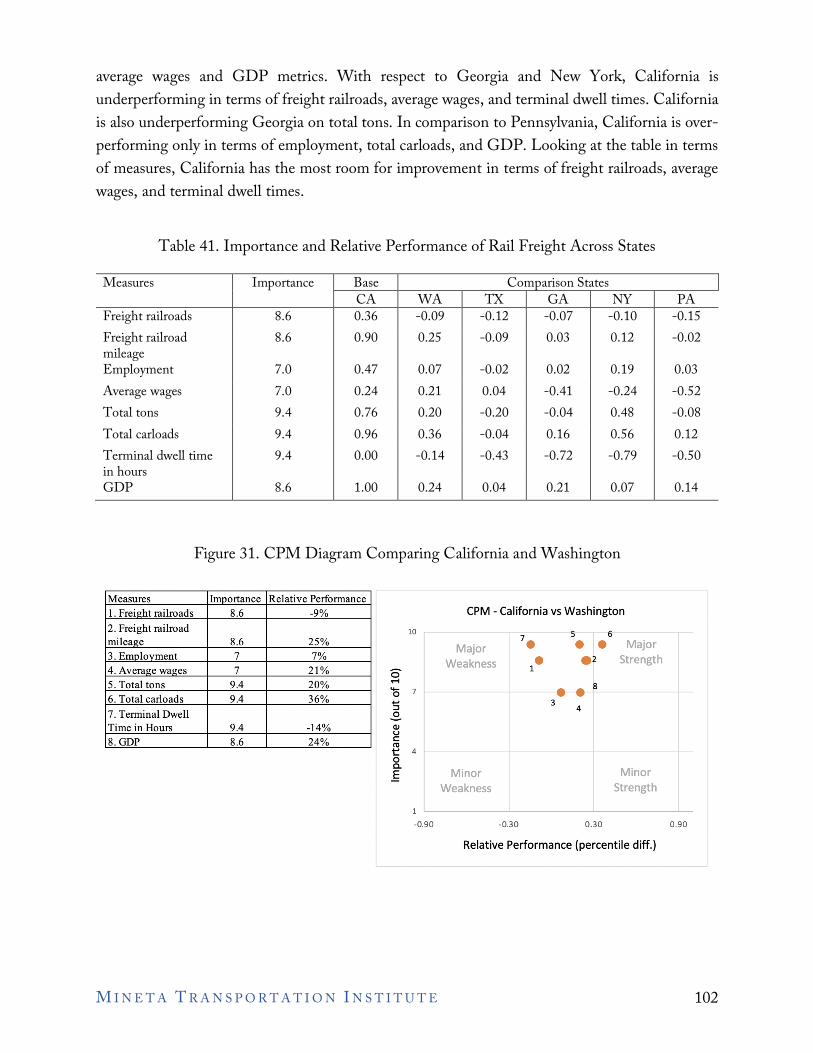
I
Measures lrnoortance Relative Performance I. Frei!!:ht railroads 8.6 -9% CPM - California vs Washington
2. Freight railroad mileage 8.6 25% 3. Emolovment 7 7% 4. Avera!!:e wa!!:es 7 21%
10 5 6
Major 7. • • Major
Weakness • e2 Strength 0 1
5. Total tons 9.4 20% 6. Total carloads 9.4 36% 7. Terminal Dwell
M 8 - 7 • • 0 ... 3 ::, 4
..2. Time in Hours 9.4 -14% QJ
u 8.GDP 8.6 24% C:
n:s t: 4 0 C.
~ Minor Minor Weakness Strength
-0.90 -0.30 0.30 0.90
Relative Performance (percentile diff.)
average wages and GDP metrics. With respect to Georgia and New York, California is underperforming in terms of freight railroads, average wages, and terminal dwell times. California is also underperforming Georgia on total tons. In comparison to Pennsylvania, California is over-performing only in terms of employment, total carloads, and GDP. Looking at the table in terms of measures, California has the most room for improvement in terms of freight railroads, average wages, and terminal dwell times.
Table 41. Importance and Relative Performance of Rail Freight Across States
Measures Importance Base Comparison States CA WA TX GA NY PA
Freight railroads 8.6 0.36 -0.09 -0.12 -0.07 -0.10 -0.15 Freight railroad 8.6 0.90 0.25 -0.09 0.03 0.12 -0.02 mileage Employment 7.0 0.47 0.07 -0.02 0.02 0.19 0.03 Average wages 7.0 0.24 0.21 0.04 -0.41 -0.24 -0.52 Total tons 9.4 0.76 0.20 -0.20 -0.04 0.48 -0.08 Total carloads 9.4 0.96 0.36 -0.04 0.16 0.56 0.12 Terminal dwell time 9.4 0.00 -0.14 -0.43 -0.72 -0.79 -0.50 in hours GDP 8.6 1.00 0.24 0.04 0.21 0.07 0.14
Figure 31. CPM Diagram Comparing California and Washington
M I N E T A T R A N S P O R T A T I O N I N S T I T U T E 102
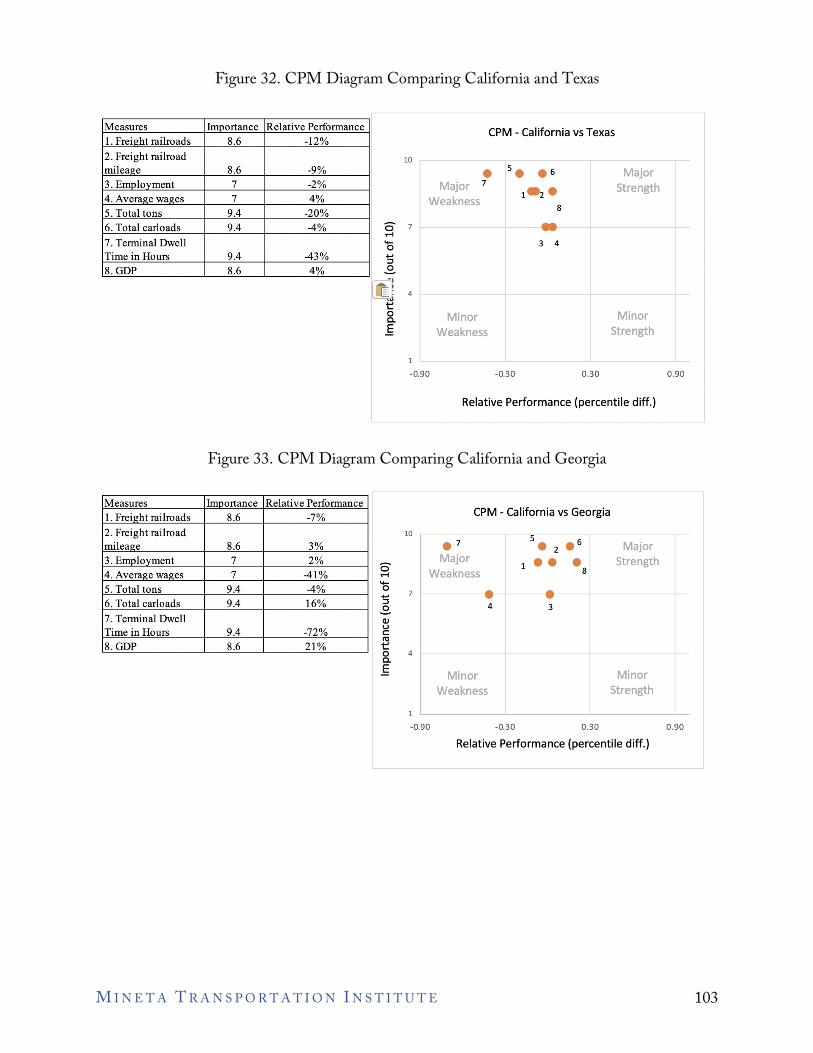
Measures Imoortance Relative Performance I. Frei2ht railroads 8.6 -12% 2. Freight railroad milea2e 8.6 -9% 3. Emolovment 7 -2% 4. Avera.,.e wa2es 7 4% 5. Total tons 9.4 -20% 6. Total carloads 9.4 -4% 7. Terminal Dwell Time in Hours 9.4 -43% 8.GDP 8.6 4%
Measures Imoortance Relative Performance I. Frei2ht railroads 8.6 -7% 2. Freight railroad milea2e 8.6 3% 3. Emnlovment 7 2% 4. Avera11:e wa2es 7 -41% 5. Total tons 9.4 -4% 6. Total carloads 9.4 16% 7. Terminal Dwell Time in Hours 9.4 -72% 8.GDP 8.6 21%
10
Major
~ Weakness
0 7 .-i -0 .... ;j
.£
CPM - California vs Texas
• 5. .6 7
1"2. 8 -3 4
Major Strength
-, IJ: 4
" t: 0 a. E
0 .-i
0 "5 .£ QI u C:
"' t: 0 a. _§
Minor Weakness
1 L__ __
-0.90 -0.30 0.30
Minor Strength
Relative Performance (percentile diff.}
CPM - california vs Georgia
10
.7
Major Weakness
Minor
• 4
1
Leakness
5 • 2 .6
1 •••
• 3
8
Major Strength
Minor Strength
0.90
-Q90 -Q30 0.30 0.90
Relative Performance (percentile diff.}
Figure 32. CPM Diagram Comparing California and Texas
Figure 33. CPM Diagram Comparing California and Georgia
M I N E T A T R A N S P O R T A T I O N I N S T I T U T E 103
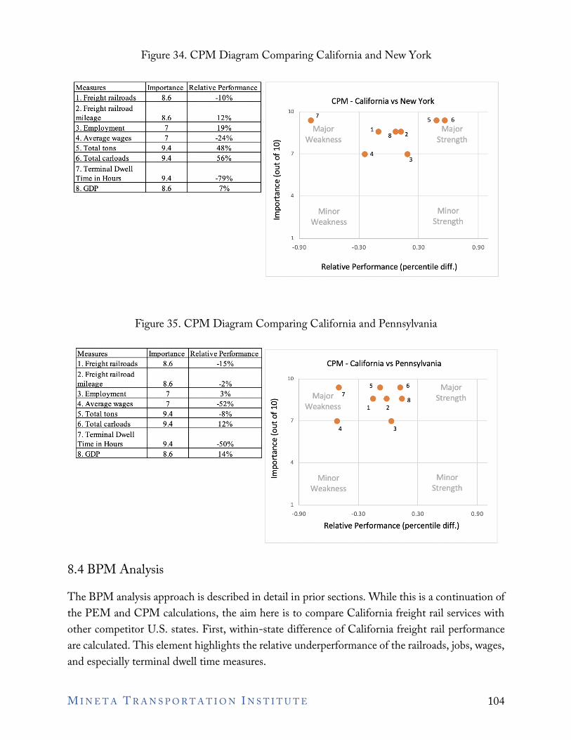
Measures Imoortance Relative Performance 1. Freight railroads 8.6 -10% CPM - California vs New York 2. Freight railroad mileage 8.6 12%
10 .7 see6
3. Emolovment 7 19% 4. Average wages 7 -24% 5. Total tons 9.4 48% 6. Total carloads 9.4 56%
Major 1. s•2 Major
0 Weakness Strength .-i - 7 .4 .3 0 ..,
7. Terminal Dwell Time in Hours 9.4 -79%
::::,
..£ QJ
8.GDP 8.6 7% u C:
"' 4 t:: 0 C. Minor Minor _§
Weakness Strength
1
-0.90 -0.30 0.30 0.90
Relative Performance (percentile diff.)
Measures Imoortance Relative Performance 1. Freight railroads 8.6 -15% CPM - California vs Pennsylvania 2. Freight railroad mileae:e 8.6 -2% 3. Emolovment 7 3% 4. Average wages 7 -52%
10
• 5. .6 Major Major 7 • • •s Strength 0 ..... Weakness 1 2
5. Total tons 9.4 -8% 6. Total carloads 9.4 12%
7. Terminal Dwell
-0 7 • • ..,
:::, 4 3 ..£
Time in Hours 9.4 -50% QI u C:
8.GDP 8.6 14% "' t:: 0 4 C.
.§ Minor Minor Weakness Strength
1
-0.90 -0.30 0.30 0.90
Relative Performance (percentile diff.)
Figure 34. CPM Diagram Comparing California and New York
Figure 35. CPM Diagram Comparing California and Pennsylvania
8.4 BPM Analysis The BPM analysis approach is described in detail in prior sections. While this is a continuation of the PEM and CPM calculations, the aim here is to compare California freight rail services with other competitor U.S. states. First, within-state difference of California freight rail performance are calculated. This element highlights the relative underperformance of the railroads, jobs, wages, and especially terminal dwell time measures.
M I N E T A T R A N S P O R T A T I O N I N S T I T U T E 104
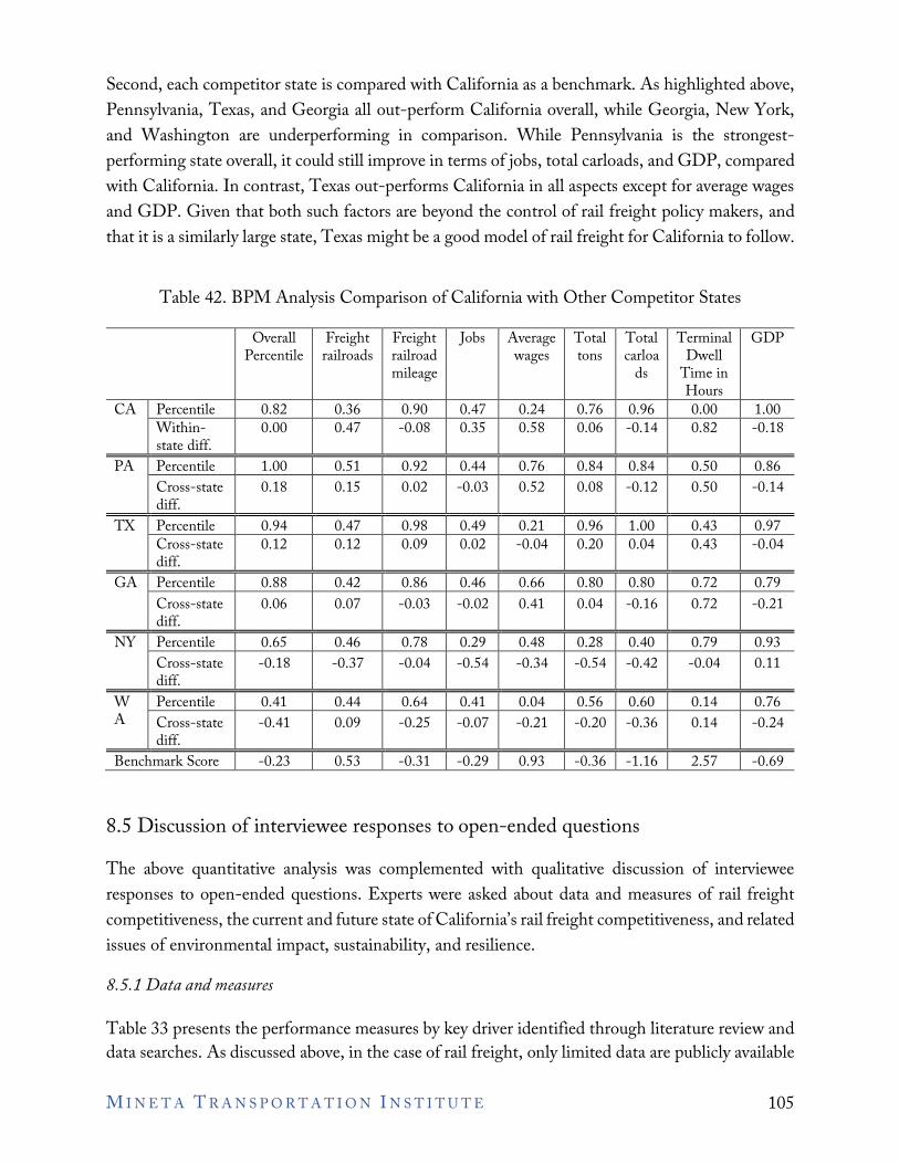
Second, each competitor state is compared with California as a benchmark. As highlighted above, Pennsylvania, Texas, and Georgia all out-perform California overall, while Georgia, New York, and Washington are underperforming in comparison. While Pennsylvania is the strongest-performing state overall, it could still improve in terms of jobs, total carloads, and GDP, compared with California. In contrast, Texas out-performs California in all aspects except for average wages and GDP. Given that both such factors are beyond the control of rail freight policy makers, and that it is a similarly large state, Texas might be a good model of rail freight for California to follow.
Table 42. BPM Analysis Comparison of California with Other Competitor States
Overall Percentile
Freight railroads
Freight railroad mileage
Jobs Average wages
Total tons
Total carloa
ds
Terminal Dwell
Time in Hours
GDP
CA Percentile 0.82 0.36 0.90 0.47 0.24 0.76 0.96 0.00 1.00 Within-state diff.
0.00 0.47 -0.08 0.35 0.58 0.06 -0.14 0.82 -0.18
PA Percentile 1.00 0.51 0.92 0.44 0.76 0.84 0.84 0.50 0.86 Cross-state diff.
0.18 0.15 0.02 -0.03 0.52 0.08 -0.12 0.50 -0.14
TX Percentile 0.94 0.47 0.98 0.49 0.21 0.96 1.00 0.43 0.97 Cross-state diff.
0.12 0.12 0.09 0.02 -0.04 0.20 0.04 0.43 -0.04
GA Percentile 0.88 0.42 0.86 0.46 0.66 0.80 0.80 0.72 0.79 Cross-state diff.
0.06 0.07 -0.03 -0.02 0.41 0.04 -0.16 0.72 -0.21
NY Percentile 0.65 0.46 0.78 0.29 0.48 0.28 0.40 0.79 0.93 Cross-state diff.
-0.18 -0.37 -0.04 -0.54 -0.34 -0.54 -0.42 -0.04 0.11
W A
Percentile 0.41 0.44 0.64 0.41 0.04 0.56 0.60 0.14 0.76 Cross-state diff.
-0.41 0.09 -0.25 -0.07 -0.21 -0.20 -0.36 0.14 -0.24
Benchmark Score -0.23 0.53 -0.31 -0.29 0.93 -0.36 -1.16 2.57 -0.69
8.5 Discussion of interviewee responses to open-ended questions The above quantitative analysis was complemented with qualitative discussion of interviewee responses to open-ended questions. Experts were asked about data and measures of rail freight competitiveness, the current and future state of California’s rail freight competitiveness, and related issues of environmental impact, sustainability, and resilience.
8.5.1 Data and measures
Table 33 presents the performance measures by key driver identified through literature review and data searches. As discussed above, in the case of rail freight, only limited data are publicly available
M I N E T A T R A N S P O R T A T I O N I N S T I T U T E 105
for many of these metrics. One area of questions in the interviews asked experts to identify additional measures that could be used to represent the key drivers.
In terms of cost, experts identified drayage and trans-loading charges, as well as inventory carrying costs as additional measures. For hinterland proximity, experts noted that rail freight tends to serve long distance routes only, with trucking serving local deliveries within 500 miles. That said, rail systems tend to serve rural areas and can also provide trans-load services, whereby container cargo is transferred from one load unit to another, usually close to a port terminal. In terms of hinterland connectivity, the efficiency and capacity of main track lines and terminals were identified as ideal metrics, as well as whether the desired cargo destination is on a developed rail intermodal route. For operational efficiency, the additional metrics suggested were consistency of transit times, and the proportional utilization of railcars. For rail service and workforce quality, numerous additional metrics were suggested by experts. These included cargo movement error rates, delays from normal transit times, and maintenance of the rail facilities by owner, appropriate measures that separate out customer service and physical service—especially where customers are “captive”, and availability of labor.
8.5.2 Current state of California freight competitiveness
In this section of questions, experts were asked about California freight rail’s competitors, game-changing investments, bottlenecks, and intermodal connections. The key U.S. competitors identified were Washington (Sea-Tac), Gulf Ports (New Orleans, Mobile etc.), and East Coast ports (competing water route via the Suez). Competition from neighboring countries—especially Canada (Prince Rupert), and Mexico west coast ports (Lazaro Cardenas)—were also noted. Within California’s freight rail system, the key connections between rail and other transportation modes were identified as ports (on-dock terminals), near dock terminals, facility tracks, and team tracks. Experts highlighted that the efficiency of these operations impact the total cost and speed of goods movement, and in turn competitiveness. Trans-loading of cargo from ports to warehouses, then to roadway and other rail hubs is also important. Experts stressed that shippers need flexibility, with key connections to ports and intermodal hubs all around U.S., with the last mile delivery undertaken on trucks. Given the importance of major highways leading to and from ports, as well as major rail yards throughout California, increased vehicular traffic decreases California’s ability to move freight. The Alameda Corridor, a submerged tripled-tracked freight rail expressway completed in 2002, along with subsequent extensions and related projects such as the Alameda Corridor East project, the San Gabriel Trench, and the Colton Crossing upgrade, were highlighted as the most impactful recent freight rail infrastructure investments in California. While these are examples of public-private partnerships involving numerous stakeholders, the majority of freight rail investments are made by the private sector, and UPRR and BNSF in particular. For example, Union Pacific double
M I N E T A T R A N S P O R T A T I O N I N S T I T U T E 106
tracked the Sunset Route to increase speeds and reduce bottlenecks. Another noted private investment was the purchase of Pacific Harbor Line territory on the ports, which facilitated cargo flows between the Ports of Long Beach and Los Angeles, and connections to inland destinations. Industry experts identified numerous bottlenecks in California’s rail system. While not directly a rail issue, the bottleneck of port container sorting and loading processes—the consequence of factors such as mega-ships and ocean carriers no longer loading boxes in destination blocks, and of alliances among carriers—has downstream impacts on rail supply lines. Upgrades to small railroad tracks that serve local markets can help to alleviate capacity issues around the ports and in regional service areas. In terms of the Class I freight railroads, competition over lines with passenger trains provide notable system bottlenecks. In particular, there are capacity limits in the Central Valley, Tehachapi and Donner pass routes. In addition to general capacity limits, mismanagement of assets and regulations were also identified as causing bottlenecks in California’s rail freight system.
8.5.3 The future of California freight rail competitiveness
To explore the future of California freight rail competitiveness, experts were asked about necessary investments and other changes needed to improve competitiveness, as well as future trends threatening competitiveness. In terms of potential investments, port infrastructure could be improved with additional near-dock capacity, zero-emission drayage systems and cargo handling systems, and inland container sorting facilities. While each of these elements is port-focused, the downstream impacts for rail freight would be significant; moreover, rail could be incorporated into these improvements. In general, experts suggested adding more infrastructure trackage adjacent to existing rail lines in areas where passenger trains share the tracks with the Class 1 Railroads. For example, the Miramar Hill (San Diego) section currently has sharp curves that limit freight rail usage yet are more acceptable for Amtrak passenger services. Straightening curves, double-tracking, or even building a tunnel through Miramar Hill could free up capacity for freight rail as well as passenger service between Los Angeles and San Diego. UPRR and BNSF have their own investment strategies to address such bottlenecks, for example, double tracks and curve smoothing on the Tehachapi pass routes. However, the state government can also play a role in identifying and analyzing bottlenecks, facilitating planning procedures, promoting public-private partnerships, and providing grants or investments where private investment is not cost-beneficial to companies, yet system-wide benefits could be experienced. One area of opportunity for California is with short lines, which require investment to increase capacity. Currently there is no sustained freight rail program for short lines, with state funds becoming available on an ad-hoc basis. Short lines may apply for the Federal Railroad Rehabilitation and Improvement Financing (RRIF) loans, but these can be restrictive. In contrast,
M I N E T A T R A N S P O R T A T I O N I N S T I T U T E 107
other states have dedicated grant or loan programs to short line investment in ties, extra rail, or new lines. There are also some bridges on short lines that cannot support new heavier trucks, and hence require upgrade investment. Short lines have been used in numerous other states such as Washington and Kansas to reduce congestion and highway degradation. There was notable discussion regarding an “inland port”, which would transport goods by rail directly from seaports to processing facilities inland. The benefits of such approaches could include more and cheaper land for operations and expansion, reduced congestion on freight-heavy freeways, reduced pollution in densely populated seaport-neighboring regions, and improved efficiencies for intermodal, trans-loading, and related services. Suggested sites for such inland ports include the “Inland Empire” region of Southern California—where there is already a substantial warehousing and distribution infrastructure—or the Central Valley. However, while the experts see projects like this happening, there are numerous obstacles, including the need for public investment, the need to cross Class I tracks, the lack of space for new tracks around the ports, and congestion around the port system during construction. One expert commented that it would require a lot of coordination and demonstration projects to prove to Class I companies that they are feasible. Other issues affecting California freight rail competitiveness include the regulation of engines, which are held to a higher standard in California than those for the Federal EPA. This could put California’s freight rail at a disadvantage compared to operations in other states. There are also notable labor issues. Similar to trucking, a particular lifestyle accompanies railroading. Despite offering high wages, the experts are reporting difficulties in finding workers willing to work 12-hour shifts, spend a long time away from home, or comply with federal cannabis regulations. On a related note, there have been proposed shifts to allow more rail automation, including one-man train crews, however, there remains hesitancy in the industry. Finally, echoing the data issues discussed above, another avenue for improved competitiveness is data sharing across the supply chain. An example for this would be the Port of L.A.’s Port Optimizer program. When considering future trends that may be major threats to California’s rail system competitiveness, experts pointed to shifting international trade patterns, technology changes, and environmental regulations. Experts observed that the shift of manufacturing operations away from China and toward the Indian Ocean threatens California’s rail volumes as it facilitates use of the competing sea lanes to the U.S. markets on the eastern seaboard that use the Suez Canal. Similarly, competition from other port regions that focus on moving cargo by rail—for example Canadian ports such as Prince Rupert—may contribute to shipments moving through such regions instead of California. This may be due to the increased reliability and increased energy-efficiency of rail. Concern was expressed that when such discretionary cargo is lost to competing regions, business is unlikely to come back, leading to a loss of money to reinvest.
M I N E T A T R A N S P O R T A T I O N I N S T I T U T E 108
8.5.4 Freight Rail Performance with respect to the Environment, Sustainability, and Resilience
Experts were asked to discuss California’s freight rail performance with respect to the environment, sustainability, and resilience. In general, experts perceived California’s rail system to be resilient to disasters. With multiple routes and cooperation between rail lines, there is little chance of a major disruption in service. It was argued that railroads have had lots of experience with major track or facility damage resulting from natural disasters in various parts of the U.S. Railroads have the capacity to quickly assess damage, assess resources needed for temporary and permanent fixes, and flow repair assets to the affected area. However, there are also legitimate concerns around fragility within the rail system due to a lack of detours or substitutes if key routes are disrupted. It was suggested that a business continuity plan would be key to getting the rail system back into operation after a disaster. When considering the environmental dimensions of freight rail, it is important to note that rail energy efficiency is far higher than other land or air transportation modes. Experts reported that while rail transports around 30 % of goods by weight, it only contributes around 2 % of emissions. Further, one current cargo train is equivalent to 750 truck trips. As such, there is a perception among industry experts that while rail should continue to improve in terms of energy efficiency— through measures such as grade separations, zero emissions vehicle terminal equipment, and advanced locomotives (Tier III and higher)—these measures are often very expensive, and regulators should be careful to not overly burden the low-emissions transportation mode. In particular, there were calls for further funding—either public or public-private partnerships—to finance lower emission locomotives or efficiency-enhancing track improvements. Environmental regulations were a notable concern, with all industry experts expressing concern that emissions regulations were constraining business, and that regulators did not tend to understand the business perspective or to whom costs would be passed on to. In particular, zero emissions mandates are challenging for freight rail. A regulation currently in development at the CA Air Resources Board (CARB) called the In-Use Locomotive Regulation, would make continued operation past 2030 financially impossible for most short line railroads and very difficult for Class 1 railroads. Away from emissions, CEQA in general is a huge burden on CA firms. It causes project timelines to extend to 5–10 years, if they can get approved at all, which means that CA firms cannot respond to market trends and opportunities with sufficient speed to take advantage of them. In contrast, project timelines in other states are much shorter.
8.6 Conclusion When competing with other U.S. modes, reliability, incidence rate, and efficiency of intermodal operations are key to the competitiveness of rail freight service. Growing demand for both passenger and freight transportation, added to capital and planning limitations for rail
M I N E T A T R A N S P O R T A T I O N I N S T I T U T E 109
infrastructure expansion, highlight the need for improved efficiency in the use of current railroad capacity (Pouryousef, Lautala, and White 2015). Privatization and vertical integration—such that railroad companies provide transportation and own the infrastructure—has contributed consistent private investment in the freight rail system over the past 40 years, which stands in contrast to publicly funded passenger rail (Furtado 2013). Any major additions to the freight rail network would require government planning authorization, and major improvements to the broader freight network such as intermodal and corridor-based planning needs to involve multiple private and public stakeholders from numerous freight modes (Guo and Peeta 2015; Sugawara 2017). For example, the State of California operates a Freight Railroad Liaison program to oversee the “planning, implementation, and monitoring of rail and rail-related capital projects with Class I Railroads, Amtrak, the Joint Powers Authorities and Local Transportation Agencies” (Caltrans 2021).
8.6..1 Findings
The PEM and CPM approaches reveal numerous insights. Data shows that California performs well in terms of freight railroad mileage, total carloads, and GDP. PEM analysis adds expert-elicited “importance” factors for which both operational efficiency and hinterland connectivity are identified as key competitiveness drivers. In the PEM analysis, California ranks 4th of the 17 states, with an overall weighted score of 40.56, and a percentile score of 82.3%. California should maintain/improve in terms of the total mileage, employment, total tons, total carloads, and GDP, and improve in terms of the number of railroads, average wages, and especially terminal dwell time. The PEM analysis also identifies the key competitor states, whereby Pennsylvania ranks the highest with an overall weighted score of 48.54, and the top percentile score. Texas (48.17; 94%) and Georgia (47.44; 88.2%) complete the top three. The BPM analysis shows that Pennsylvania, Texas, and Georgia are all out-performing California overall. In contrast, Georgia, New York, and Washington are all underperforming California. Pennsylvania appears to be the strongest-performing state overall, yet it lags behind California in terms of jobs, total carloads, and GDP. Texas out-performs California in all metrics except for average wages and GDP. As both factors are beyond the control of rail freight policy makers, and it is a similarly large state, Texas might be a good model for California to follow when considering rail freight improvements. When considering the current state of California freight rail competitiveness, experts identified connections with the ports and intermodal hubs as critical. Major infrastructure projects such as the Alameda Corridor and related projects, the Pacific Harbor Line have improved competitiveness significantly, as have ongoing investments by BNSF and UPRR.
M I N E T A T R A N S P O R T A T I O N I N S T I T U T E 110
8.6.2 Suggestions
Bottlenecks at the ports, as well as capacity issues on some bridges, and in the Central Valley, Tehachapi, and Donner pass, may all be invested in to improve competitiveness further. Other major infrastructure projects such as “inland ports” and other short line projects to add capacity and alleviate congestion in port-neighboring regions could significantly improve competitiveness but would require public investment or public-private financing to be realized due to insufficient payoffs for private investors. Short lines also offer significant promise, especially when dedicated state support has been provided through targeted grant and loan programs. While experts generally considered California’s freight rail system to be resilient to disasters, concerns were raised regarding the environmental regulations facing the industry. There is a concern that emissions regulations in particular were constraining business, and that regulators did not tend to understand the business perspective or to whom costs would be passed on to. Industry experts expressed that while rail should continue to improve in terms of energy efficiency—through measures such as grade separations, zero emissions vehicle terminal equipment, and advanced locomotives (Tier III and higher)—these measures are often very expensive, and regulators should be careful to not overly burden a low-emissions transportation mode. There were calls for further funding—either public or public-private partnerships—to finance lower emission locomotives or efficiency-enhancing track improvements. 8.6.3 Workforce Development Plan The railroad industry is experiencing similar workforce issues to other industries, including aging workers, shifting expectations around work-life balance, and changing educational systems. In response to the aging workforce, the railroad industry has been recruiting military veterans, with 20 % of current U.S. railroad employees being veterans. In terms of educational preparation, some community colleges—including Sacramento City College and San Diego City College—have developed Railroad Operations associate degrees and certificate programs. The San Diego program notably incorporates an apprenticeship, with contributions from organizations such as the International Union of Operating Engineers and the Teamsters Apprenticeship Fund for Southern California. The apprenticeship model is ideal for the recommended infrastructure construction and automation changes required to enhance our competitiveness. Automation and working with environmental issues must be marketed to the potential workforce as career opportunities, rather than leading to job displacement. Local economic and workforce boards, and community-based organizations, who are in touch with underrepresented and often underemployed or unemployed populations, can provide excellent channels to meet workforce needs and overcome typical work/life balance issues in this sector.
M I N E T A T R A N S P O R T A T I O N I N S T I T U T E 111
9. Distribution Centers 9.1 Introduction The trends of population, employment, and economy are the primary factors affecting the demand and supply of industrial land. Table 43 reports the 2005–2019 annual growth rates and shares of real GDP, population, and employment in the top 25 U.S. metropolitan areas. Figure 36 presents the year-over-year growth trend of major U.S. metropolitan areas and Table 44 summarizes the statistics of California’s top 10 metropolitan areas. The demographic statistics in Tables 43 and 44 and Figure 36 provide important critical insights. First, large metropolitan areas are losing shares in terms of populations and employment to emerging metropolitan areas. This trend implies there is a more substantial demand for land in those emerging regions. For example, compared with the U.S.’ annual growth rate of 0.87% in population during 2005–2019, the New York-Newark and Los Angeles metropolitan areas grew only 0.25% and 0.27% in compounded annual growth rate (CAGR), respectively. In contrast, Dallas (TX) and Houston (TX) populations surged 2.02% and 2.17%, respectively, every year. Seattle (WA), Atlanta (GA), and Phoenix (AZ) have more than 1.5% CAGR. Recent moves of high-tech firms are evidence of this trend. For example, software giant Oracle moved its corporate headquarter from Silicon Valley to Austin, Texas. Likewise, Hewlett Packard Enterprise relocated its headquarters from San Jose to Houston. Second, the differences in the growth rates between real GDP and population show the sources of growth and distinct industry profiles of metropolitan areas. The U.S. growth rate of real GDP (1.7%) is generally higher than that of the population (0.87%), leading to an increase in the GDP per capita. In the metropolitan areas, the GDP growth is contributed to by increases in productivity and/or populations. For example, San Francisco and San Jose have higher growth rates in real GDP at 3.5% and 6.6%, respectively, than the U.S. average without a noticeable growth in population, implying a productivity-driven growth in GDP. In contrast, the differences between the growth rates of real GDP and population are smaller for the emerging metropolitan areas like Dallas, Houston, and Atlanta, implying that the GDP growth is mainly contributed to by population growth due to more start-up business and move-in companies. Third, Table 44 shows that some of California’s emerging metropolitan areas like Riverside-San Bernardino-Ontario and Bakersfield have grown in the past 15 years. The main reasons for the growth include lower rent and wage costs, and the surge of demand for e-commerce. The rent for the inland empire counties is 35% lower when compared to Los Angeles and Orange County in 2020 (Cushman and Wakefield 2021).
M I N E T A T R A N S P O R T A T I O N I N S T I T U T E 112
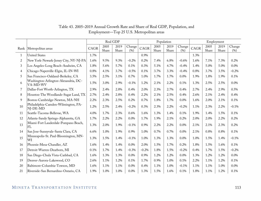
Table 43. 2005–2019 Annual Growth Rate and Share of Real GDP, Population, and Employment—Top 25 U.S. Metropolitan areas
Rank Metropolitan areas Real GDP Population Employment
CAGR 2005 2019 Share Share
Change (%) CAGR 2005 2019
Share Share Change
(%) CAGR 2005 2019 Share Share
Change (%)
1 United States 2 New York-Newark-Jersey City, NY-NJ-PA 3 Los Angeles-Long Beach-Anaheim, CA 4 Chicago-Naperville-Elgin, IL-IN-WI 5 San Francisco-Oakland-Berkeley, CA
Washington-Arlington-Alexandria, DC-6 VA-MD-WV 7 Dallas-Fort Worth-Arlington, TX 8 Houston-The Woodlands-Sugar Land, TX 9 Boston-Cambridge-Newton, MA-NH
Philadelphia-Camden-Wilmington, PA-10 NJ-DE-MD 11 Seattle-Tacoma-Bellevue, WA 12 Atlanta-Sandy Springs-Alpharetta, GA
Miami-Fort Lauderdale-Pompano Beach, 13 FL 14 San Jose-Sunnyvale-Santa Clara, CA
Minneapolis-St. Paul-Bloomington, MN-15 WI 16 Phoenix-Mesa-Chandler, AZ 17 Detroit-Warren-Dearborn, MI 18 San Diego-Chula Vista-Carlsbad, CA 19 Denver-Aurora-Lakewood, CO 20 Baltimore-Columbia-Towson, MD 21 Riverside-San Bernardino-Ontario, CA
1.7% 1.6% 1.8% 0.8% 3.5% 1.5% 2.9% 2.7% 2.2% 1.2% 4.0% 1.7% 1.3% 6.6% 1.3% 1.6% 0.1% 1.6% 2.6% 1.6% 1.9%
9.5% 9.3% 5.6% 5.7% 4.1% 3.7% 2.5% 3.1% 3.0% 2.9% 2.4% 2.8% 2.4% 2.8% 2.3% 2.5% 2.5% 2.4% 1.7% 2.3% 2.2% 2.2% 2.0% 1.9% 1.0% 1.9% 1.5% 1.4% 1.4% 1.4% 1.7% 1.4% 1.3% 1.3% 1.1% 1.2% 1.1% 1.1% 1.0% 1.0%
-0.2% 0.1% -0.5% 0.7% -0.1% 0.4% 0.4% 0.2% -0.2% 0.6% 0.0% -0.1% 0.9% -0.1% 0.0% -0.3% 0.0% 0.1% 0.0% 0.0%
0.9% 0.2% 0.3% 0.1% 1.0% 1.2% 2.0% 2.2% 0.7% 0.3% 1.6% 1.7% 0.9% 1.0% 1.0% 2.0% -0.2% 0.9% 1.7% 0.4% 1.3%
7.4% 6.8% 5.1% 4.7% 3.7% 3.3% 1.7% 1.7% 2.1% 2.2% 2.3% 2.7% 2.1% 2.5% 1.8% 1.7% 2.3% 2.2% 1.3% 1.4% 1.9% 2.1% 2.2% 2.2% 0.7% 0.7% 1.3% 1.3% 1.5% 1.7% 1.8% 1.5% 1.2% 1.2% 0.9% 1.0% 1.1% 1.0% 1.5% 1.6%
-0.6% -0.4% -0.4% 0.0% 0.1% 0.4% 0.4% 0.0% -0.2% 0.1% 0.2% 0.0% 0.0% 0.0% 0.2% -0.2% 0.0% 0.1% -0.1% 0.1%
1.3% 1.6% 1.4% 0.8% 1.9% 1.3% 2.7% 2.6% 1.6% 1.1% 1.9% 2.0% 2.1% 2.1% 1.0% 1.8% 0.4% 1.3% 2.2% 1.1% 1.8%
7.1% 7.3% 5.0% 5.0% 3.7% 3.5% 1.8% 1.9% 2.5% 2.5% 2.4% 2.9% 2.1% 2.4% 2.0% 2.1% 2.3% 2.2% 1.4% 1.5% 2.0% 2.2% 2.1% 2.3% 0.8% 0.8% 1.5% 1.4% 1.5% 1.6% 1.7% 1.5% 1.2% 1.2% 1.1% 1.2% 1.1% 1.0% 1.1% 1.2%
0.2% 0.0% -0.2% 0.1% 0.0% 0.5% 0.4% 0.1% -0.1% 0.1% 0.2% 0.2% 0.1% -0.1% 0.1% -0.2% 0.0% 0.1% 0.0% 0.1%
M I N E T A T R A N S P O R T A T I O N I N S T I T U T E 113
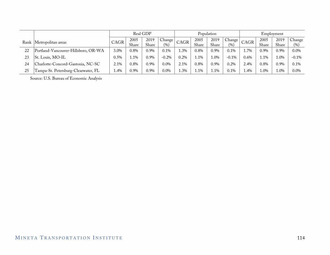
Rank Metropolitan areas Real GDP Population Employment
CAGR 2005 Share
2019 Share
Change (%) CAGR 2005
Share 2019 Share
Change (%) CAGR 2005
Share 2019 Share
Change (%)
22 Portland-Vancouver-Hillsboro, OR-WA 3.0% 0.8% 0.9% 0.1% 1.3% 0.8% 0.9% 0.1% 1.7% 0.9% 0.9% 0.0% 23 St. Louis, MO-IL 0.5% 1.1% 0.9% -0.2% 0.2% 1.1% 1.0% -0.1% 0.6% 1.1% 1.0% -0.1% 24 Charlotte-Concord-Gastonia, NC-SC 2.1% 0.8% 0.9% 0.0% 2.1% 0.8% 0.9% 0.2% 2.4% 0.8% 0.9% 0.1% 25 Tampa-St. Petersburg-Clearwater, FL 1.4% 0.9% 0.9% 0.0% 1.3% 1.1% 1.1% 0.1% 1.4% 1.0% 1.0% 0.0%
Source: U.S. Bureau of Economic Analysis
M I N E T A T R A N S P O R T A T I O N I N S T I T U T E 114
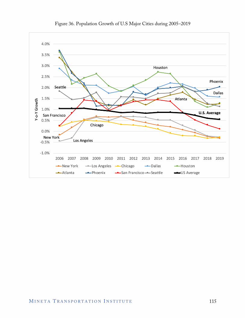
~ 0 ...
I!)
> 6 >-
4.0%
3.5%
3.0%
2.5% Phoenix
2.0%
1.5%
1.0%
San Francisco 0.5%
0.0%
-0.5%
-1.0% 2006 2007 2008 2009 2010 2011 2012 2013 2014 2015 2016 2017 2018 2019
.-New York
--Atlanta
.-Los Angeles .-Chicago --Dallas
.-Phoenix .-san Francisco.-seattle
.-Houston
-us Average
..c
Figure 36. Population Growth of U.S Major Cities during 2005–2019
M I N E T A T R A N S P O R T A T I O N I N S T I T U T E 115
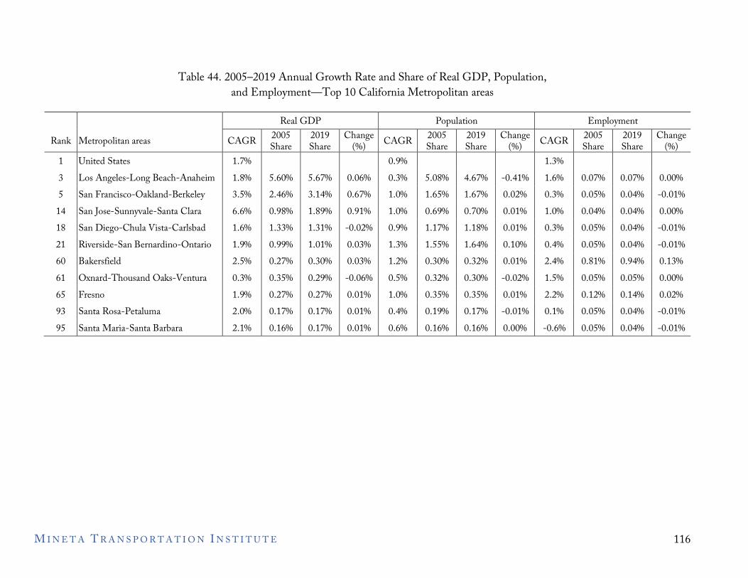
Table 44. 2005–2019 Annual Growth Rate and Share of Real GDP, Population, and Employment—Top 10 California Metropolitan areas
Rank Metropolitan areas Real GDP Population Employment
CAGR 2005 Share
2019 Share
Change (%) CAGR 2005
Share 2019 Share
Change (%) CAGR 2005
Share 2019 Share
Change (%)
1 United States 1.7% 0.9% 1.3% 3 Los Angeles-Long Beach-Anaheim 1.8% 5.60% 5.67% 0.06% 0.3% 5.08% 4.67% -0.41% 1.6% 0.07% 0.07% 0.00% 5 San Francisco-Oakland-Berkeley 3.5% 2.46% 3.14% 0.67% 1.0% 1.65% 1.67% 0.02% 0.3% 0.05% 0.04% -0.01%
14 San Jose-Sunnyvale-Santa Clara 6.6% 0.98% 1.89% 0.91% 1.0% 0.69% 0.70% 0.01% 1.0% 0.04% 0.04% 0.00% 18 San Diego-Chula Vista-Carlsbad 1.6% 1.33% 1.31% -0.02% 0.9% 1.17% 1.18% 0.01% 0.3% 0.05% 0.04% -0.01% 21 Riverside-San Bernardino-Ontario 1.9% 0.99% 1.01% 0.03% 1.3% 1.55% 1.64% 0.10% 0.4% 0.05% 0.04% -0.01% 60 Bakersfield 2.5% 0.27% 0.30% 0.03% 1.2% 0.30% 0.32% 0.01% 2.4% 0.81% 0.94% 0.13% 61 Oxnard-Thousand Oaks-Ventura 0.3% 0.35% 0.29% -0.06% 0.5% 0.32% 0.30% -0.02% 1.5% 0.05% 0.05% 0.00% 65 Fresno 1.9% 0.27% 0.27% 0.01% 1.0% 0.35% 0.35% 0.01% 2.2% 0.12% 0.14% 0.02% 93 Santa Rosa-Petaluma 2.0% 0.17% 0.17% 0.01% 0.4% 0.19% 0.17% -0.01% 0.1% 0.05% 0.04% -0.01% 95 Santa Maria-Santa Barbara 2.1% 0.16% 0.17% 0.01% 0.6% 0.16% 0.16% 0.00% -0.6% 0.05% 0.04% -0.01%
M I N E T A T R A N S P O R T A T I O N I N S T I T U T E 116
The booming e-commerce and m-commerce (mobile) have dramatically transformed the retail sector and land use. For example, in the first quarter of 2021, the estimated e-commerce sales increased 39.1% from the first quarter of 2020, while total retail sales increased 16.8% in the same period. As a result, e-commerce sales accounted for 13.6% of total sales in the U.S. (U.S. Census Bureau 2021). Traditional retailers found it more cost-effective by adding an online option than opening more brick-and-mortar stores. CBRE, a commercial real estate firm, indicated that one third of all demand for "big-box" distribution and logistics space (>400,000 square feet) is tied to multi-channel retailers or "e-tailers" who sell products and services to customers completely using online stores (Thompson and Carver 2021). Demand for e-commerce retailers has been growing since 2009. While 21 North American retailers filed for bankruptcy in 2020 because of the COVID-19 pandemic, consumers spent $861.12 billion online in 2020, up 44% from $598.02 billion in 2019 (Ali 2021). In addition, Amazon dominates the U.S. e-commerce market and accounts for 40.4% of total e-commerce sales, followed by Walmart’s 7.1% and eBay’s 4.3% in 2021 (eMarketer, February 2021). Table 45 reports the numbers and percentages of Amazon’s fulfillment centers in the U.S. Amazon operations are concentrated in four states: California, Texas, Kentucky, and Pennsylvania. California owns the largest number and capacity of the fulfillment centers in the U.S. Table 46 shows that Los Angeles-Long Beach-Anaheim and Riverside-San Bernardino-Ontario metropolitan areas account for about 55% of Amazon’s operations in California.
M I N E T A T R A N S P O R T A T I O N I N S T I T U T E 117
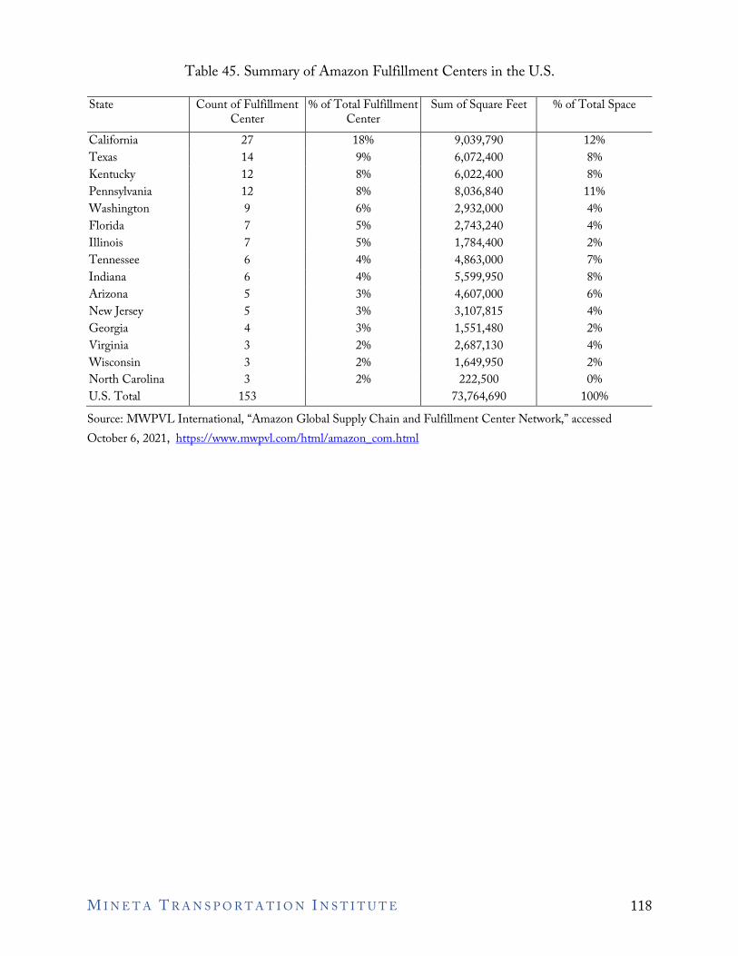
Table 45. Summary of Amazon Fulfillment Centers in the U.S.
State Count of Fulfillment Center
% of Total Fulfillment Center
Sum of Square Feet % of Total Space
California 27 18% 9,039,790 12% Texas 14 9% 6,072,400 8% Kentucky 12 8% 6,022,400 8% Pennsylvania 12 8% 8,036,840 11% Washington 9 6% 2,932,000 4% Florida 7 5% 2,743,240 4% Illinois 7 5% 1,784,400 2% Tennessee 6 4% 4,863,000 7% Indiana 6 4% 5,599,950 8% Arizona 5 3% 4,607,000 6% New Jersey 5 3% 3,107,815 4% Georgia 4 3% 1,551,480 2% Virginia 3 2% 2,687,130 4% Wisconsin 3 2% 1,649,950 2% North Carolina 3 2% 222,500 0% U.S. Total 153 73,764,690 100% Source: MWPVL International, “Amazon Global Supply Chain and Fulfillment Center Network,” accessed October 6, 2021, https://www.mwpvl.com/html/amazon_com.html
M I N E T A T R A N S P O R T A T I O N I N S T I T U T E 118
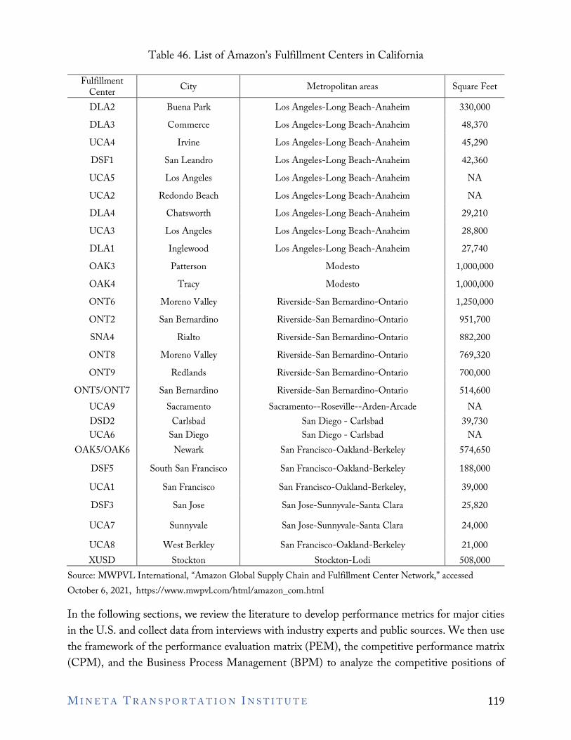
Table 46. List of Amazon’s Fulfillment Centers in California
Fulfillment Center City Metropolitan areas Square Feet DLA2 Buena Park Los Angeles-Long Beach-Anaheim 330,000 DLA3 Commerce Los Angeles-Long Beach-Anaheim 48,370 UCA4 Irvine Los Angeles-Long Beach-Anaheim 45,290 DSF1 San Leandro Los Angeles-Long Beach-Anaheim 42,360 UCA5 Los Angeles Los Angeles-Long Beach-Anaheim NA UCA2 Redondo Beach Los Angeles-Long Beach-Anaheim NA DLA4 Chatsworth Los Angeles-Long Beach-Anaheim 29,210 UCA3 Los Angeles Los Angeles-Long Beach-Anaheim 28,800 DLA1 Inglewood Los Angeles-Long Beach-Anaheim 27,740 OAK3 Patterson Modesto 1,000,000 OAK4 Tracy Modesto 1,000,000 ONT6 Moreno Valley Riverside-San Bernardino-Ontario 1,250,000 ONT2 San Bernardino Riverside-San Bernardino-Ontario 951,700 SNA4 Rialto Riverside-San Bernardino-Ontario 882,200 ONT8 Moreno Valley Riverside-San Bernardino-Ontario 769,320 ONT9 Redlands Riverside-San Bernardino-Ontario 700,000
ONT5/ONT7 San Bernardino Riverside-San Bernardino-Ontario 514,600 UCA9 Sacramento Sacramento--Roseville--Arden-Arcade NA DSD2 Carlsbad San Diego - Carlsbad 39,730 UCA6 San Diego San Diego - Carlsbad NA
OAK5/OAK6 Newark San Francisco-Oakland-Berkeley 574,650 DSF5 South San Francisco San Francisco-Oakland-Berkeley 188,000 UCA1 San Francisco San Francisco-Oakland-Berkeley, 39,000 DSF3 San Jose San Jose-Sunnyvale-Santa Clara 25,820 UCA7 Sunnyvale San Jose-Sunnyvale-Santa Clara 24,000 UCA8 West Berkley San Francisco-Oakland-Berkeley 21,000 XUSD Stockton Stockton-Lodi 508,000
Source: MWPVL International, “Amazon Global Supply Chain and Fulfillment Center Network,” accessed October 6, 2021, https://www.mwpvl.com/html/amazon_com.html
In the following sections, we review the literature to develop performance metrics for major cities in the U.S. and collect data from interviews with industry experts and public sources. We then use the framework of the performance evaluation matrix (PEM), the competitive performance matrix (CPM), and the Business Process Management (BPM) to analyze the competitive positions of
M I N E T A T R A N S P O R T A T I O N I N S T I T U T E 119
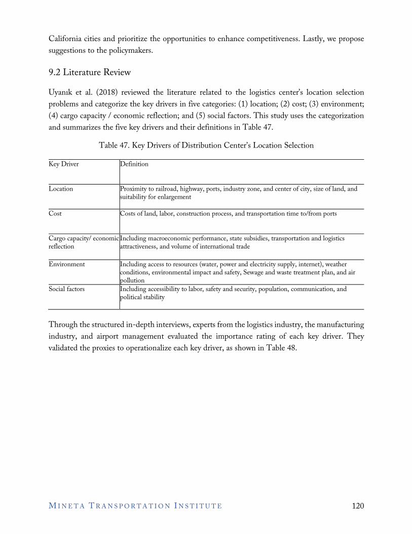
California cities and prioritize the opportunities to enhance competitiveness. Lastly, we propose suggestions to the policymakers.
9.2 Literature Review Uyanık et al. (2018) reviewed the literature related to the logistics center’s location selection problems and categorize the key drivers in five categories: (1) location; (2) cost; (3) environment; (4) cargo capacity / economic reflection; and (5) social factors. This study uses the categorization and summarizes the five key drivers and their definitions in Table 47.
Table 47. Key Drivers of Distribution Center’s Location Selection
Key Driver Definition
Location Proximity to railroad, highway, ports, industry zone, and center of city, size of land, and suitability for enlargement
Cost Costs of land, labor, construction process, and transportation time to/from ports
Cargo capacity/ economic reflection
Including macroeconomic performance, state subsidies, transportation and logistics attractiveness, and volume of international trade
Environment Including access to resources (water, power and electricity supply, internet), weather conditions, environmental impact and safety, Sewage and waste treatment plan, and air pollution
Social factors Including accessibility to labor, safety and security, population, communication, and political stability
Through the structured in-depth interviews, experts from the logistics industry, the manufacturing industry, and airport management evaluated the importance rating of each key driver. They validated the proxies to operationalize each key driver, as shown in Table 48.
M I N E T A T R A N S P O R T A T I O N I N S T I T U T E 120
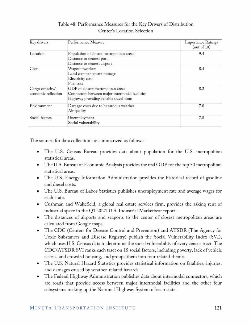
Table 48. Performance Measures for the Key Drivers of Distribution Center’s Location Selection
Key drivers Performance Measure Importance Ratings (out of 10)
Location Population of closest metropolitan areas Distance to nearest port Distance to nearest airport
9.4
Cost Wages—workers Land cost per square footage Electricity cost Fuel cost
8.4
Cargo capacity/ economic reflection
GDP of closest metropolitan areas Connectors between major intermodal facilities Highway providing reliable travel time
8.2
Environment Damage costs due to hazardous weather Air quality
7.0
Social factors Unemployment Social vulnerability
7.8
The sources for data collection are summarized as follows:
• The U.S. Census Bureau provides data about population for the U.S. metropolitan statistical areas.
• The U.S. Bureau of Economic Analysis provides the real GDP for the top 50 metropolitan statistical areas.
• The U.S. Energy Information Administration provides the historical record of gasoline and diesel costs.
• The U.S. Bureau of Labor Statistics publishes unemployment rate and average wages for each state.
• Cushman and Wakefield, a global real estate services firm, provides the asking rent of industrial space in the Q1-2021 U.S. Industrial Marketbeat report.
• The distances of airports and seaports to the center of closest metropolitan areas are calculated from Google maps.
• The CDC (Centers for Disease Control and Prevention) and ATSDR (The Agency for Toxic Substances and Disease Registry) publish the Social Vulnerability Index (SVI), which uses U.S. Census data to determine the social vulnerability of every census tract. The CDC/ATSDR SVI ranks each tract on 15 social factors, including poverty, lack of vehicle access, and crowded housing, and groups them into four related themes.
• The U.S. Natural Hazard Statistics provides statistical information on fatalities, injuries, and damages caused by weather-related hazards.
• The Federal Highway Administration publishes data about intermodal connectors, which are roads that provide access between major intermodal facilities and the other four subsystems making up the National Highway System of each state.
M I N E T A T R A N S P O R T A T I O N I N S T I T U T E 121
9.3 PEM and CPM Analyses In this section, we employed the Performance Evaluation Matrix (PEM) and Competitive Performance Matrix (CPM) and analyzed the competitive position of California cities. First, Section 9.3.1 reports data used for the cross-city comparison. Second, Section 9.3.2 uses the PEM approach to analyze California city’s strengths and weaknesses. In Section 9.3.3, the CPM analysis reveals California’s composition relative to competing cities. The CPM consists of the differences in the performance percentile between the focal city and compared cities and the importance rating for each performance measure.
9.3.1 Data
This section summarizes the data collected from multiple public sources for the performance measures for major U.S. cities, as shown in Table 49. Table 50 reports the performance percentile of each city and the importance rating for each performance measure. The overall weighted score for a city is calculated as the product of importance ratings and performance percentiles. Lastly, Table 51 reports the ranking of major U.S. cities based on overall weighted scores. According to the overall weighted scores in Table 51, the top five cities in the U.S. are:
(1) Tampa, FL (2) Houston, TX (3) Atlanta, GA (4) Newark NJ (5) Seattle, WA
In addition to these five cities, industry experts mentioned that the major cities such as Los Angeles, San Francisco, and San Jose in California are competing with Phoenix, AZ and Las Vegas, NV. Hence, we include seven cities in the competitive analysis.
M I N E T A T R A N S P O R T A T I O N I N S T I T U T E 122
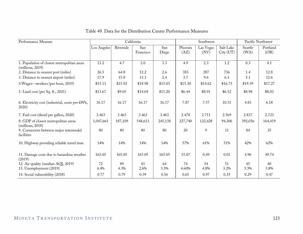
Table 49. Data for the Distribution Center Performance Measures
Performance Measure California Southwest Pacific Northwest Los Angeles Riverside San
Francisco San
Diego Phoenix
(AZ) Las Vegas
(NV) Salt Lake City (UT)
Seattle (WA)
Portland (OR)
1. Population of closest metropolitan areas (millions, 2019)
13.2 4.7 2.0 3.3 4.9 2.3 1.2 0.3 0.1
2. Distance to nearest port (miles) 26.5 64.8 12.2 2.6 383 287 736 1.4 12.8 3. Distance to nearest airport (miles) 17.9 15.8 13.3 2.4 3.7 9.6 6.1 5.1 12.6 4.Wages—workers (per hour, 2019) $15.13 $15.92 $18.98 $15.03 $15.30 $14.62 $16.73 $19.39 $17.27 5. Land cost (per Sq. ft., 2021) $13.67 $9.05 $14.69 $11.20 $6.44 $8.91 $6.52 $8.98 $8.03
6. Electricity cost (industrial, cents per kWh, 2020)
16.17 16.17 16.17 16.17 7.87 7.57 10.31 4.83 6.18
7. Fuel cost (diesel per gallon, 2020) 3.463 3.463 3.463 3.463 2.478 2.711 2.569 2.837 2.723 8. GDP of closest metropolitan areas (millions, 2018)
1,047,661 187,109 548,613 245,138 227,740 122,428 94,306 392,036 164,419
9. Connectors between major intermodal facilities
80 80 80 80 20 9 11 84 35
10. Highway providing reliable travel time 14% 14% 14% 14% 57% 61% 51% 42% 62%
11. Damage costs due to hazardous weather (2019)
165.05 165.05 165.05 165.05 15.07 0.49 0.01 4.96 49.74
12. Air quality (median AQI, 2019) 72 89 43 64 74 54 51 45 40 13. Unemployment (2019) 4.4% 4.3% 2.6% 3.5% 4.60% 4.8% 3.2% 3.3% 3.8% 14. Social vulnerability (2018) 0.77 0.79 0.39 0.56 0.65 0.97 0.35 0.29 0.47
M I N E T A T R A N S P O R T A T I O N I N S T I T U T E 123
Table 49. Data for the Distribution Center Performance Measures (Continued)
Performance Measure Texas and South Central Southeast and South Atlantic Northeast Dallas (TX)
Houston (TX)
Austin (TX)
Miami (FL)
Tampa (FL)
Atlanta (GA)
Baltimore (MD)
Newark (NJ)
Boston (MA)
Phila-delphia
(PA) 1. Population of closest metropolitan areas 0.1 7.1 2.2 0.5 3.2 0.2 2.8 19.2 1.6 0.4 2. Distance to nearest port 247 15.7 171 2.7 8.9 250 0.5 3.6 2.5 5.7 3. Distance to nearest airport 20.2 23.2 9.6 8.9 7.7 8.4 10.1 6.4 2.5 11.3 4.Wages—workers $16.56 $15.72 $15.10 $14.26 $13.80 $14.97 $15.93 $16.71 $16.84 $15.53 5. Land cost $4.69 $5.84 $10.26 $8.56 $5.40 $6.43 $5.88 $10.51 $7.45 $6.72 6. Electricity cost 5.09 5.09 5.09 7.15 7.15 5.71 7.59 10.52 13.87 6.08 7. Fuel cost 2.212 2.212 2.212 2.541 2.541 2.485 2.792 2.675 2.792 2.922 8. GDP of closest metropolitan areas 512,509 478,778 146,784 354,740 159,002 397,261 205,313 1,772,319 463,570 444,148 9. Connectors between major intermodal 191 191 191 58 58 64 56 56 111 73 facilities 10. Highway providing reliable travel time 44% 44% 44% 30% 30% 47% 18% 22% 30% 77% 11. Damage costs due to hazardous weather 3,100.52 3,100.52 3,100.52 27.58 27.58 20.95 2.27 0.93 2.27 31.70 12. Air quality 51 52 44 41 43 52 46 51 43 51 13. Unemployment 3.4% 3.7% 2.5% 3.4% 3.3% 4.0% 5.3% 6.7% 2.5% 4.6% 14. Social vulnerability 0.75 0.72 0.38 0.82 0.67 0.53 0.83 0.84 0.74 0.92
M I N E T A T R A N S P O R T A T I O N I N S T I T U T E 124
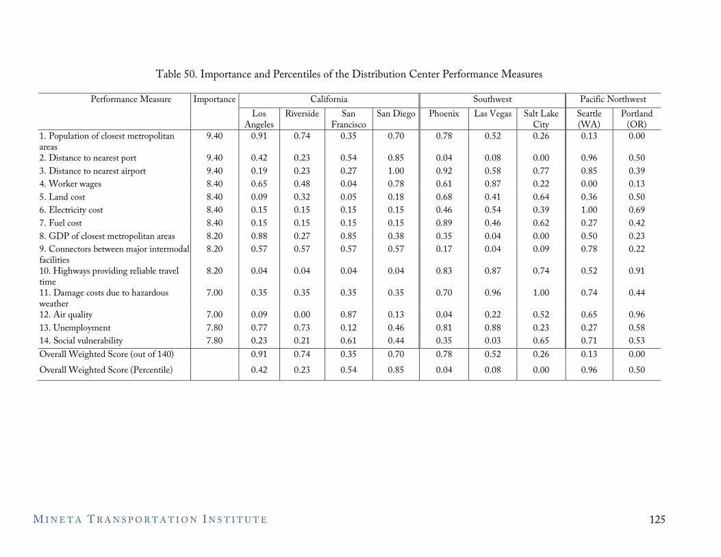
Table 50. Importance and Percentiles of the Distribution Center Performance Measures
Performance Measure Importance California Southwest Pacific Northwest Los
Angeles Riverside San
Francisco San Diego Phoenix Las Vegas Salt Lake
City Seattle (WA)
Portland (OR)
1. Population of closest metropolitan 9.40 0.91 0.74 0.35 0.70 0.78 0.52 0.26 0.13 0.00 areas 2. Distance to nearest port 9.40 0.42 0.23 0.54 0.85 0.04 0.08 0.00 0.96 0.50 3. Distance to nearest airport 9.40 0.19 0.23 0.27 1.00 0.92 0.58 0.77 0.85 0.39 4. Worker wages 8.40 0.65 0.48 0.04 0.78 0.61 0.87 0.22 0.00 0.13 5. Land cost 8.40 0.09 0.32 0.05 0.18 0.68 0.41 0.64 0.36 0.50 6. Electricity cost 8.40 0.15 0.15 0.15 0.15 0.46 0.54 0.39 1.00 0.69 7. Fuel cost 8.40 0.15 0.15 0.15 0.15 0.89 0.46 0.62 0.27 0.42 8. GDP of closest metropolitan areas 8.20 0.88 0.27 0.85 0.38 0.35 0.04 0.00 0.50 0.23 9. Connectors between major intermodal 8.20 0.57 0.57 0.57 0.57 0.17 0.04 0.09 0.78 0.22 facilities 10. Highways providing reliable travel 8.20 0.04 0.04 0.04 0.04 0.83 0.87 0.74 0.52 0.91 time 11. Damage costs due to hazardous 7.00 0.35 0.35 0.35 0.35 0.70 0.96 1.00 0.74 0.44 weather 12. Air quality 7.00 0.09 0.00 0.87 0.13 0.04 0.22 0.52 0.65 0.96 13. Unemployment 7.80 0.77 0.73 0.12 0.46 0.81 0.88 0.23 0.27 0.58 14. Social vulnerability 7.80 0.23 0.21 0.61 0.44 0.35 0.03 0.65 0.71 0.53 Overall Weighted Score (out of 140) Overall Weighted Score (Percentile)
0.91 0.42
0.74 0.23
0.35 0.54
0.70 0.85
0.78 0.04
0.52 0.08
0.26 0.00
0.13 0.96
0.00 0.50
M I N E T A T R A N S P O R T A T I O N I N S T I T U T E 125
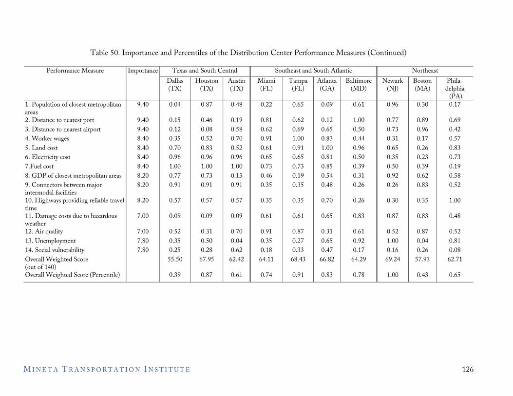
Table 50. Importance and Percentiles of the Distribution Center Performance Measures (Continued)
Performance Measure Importance Texas and South Central Southeast and South Atlantic Northeast Dallas (TX)
Houston (TX)
Austin (TX)
Miami (FL)
Tampa (FL)
Atlanta (GA)
Baltimore (MD)
Newark (NJ)
Boston (MA)
Phila-delphia
(PA) 1. Population of closest metropolitan areas
9.40 0.04 0.87 0.48 0.22 0.65 0.09 0.61 0.96 0.30 0.17
2. Distance to nearest port 9.40 0.15 0.46 0.19 0.81 0.62 0.12 1.00 0.77 0.89 0.69 3. Distance to nearest airport 9.40 0.12 0.08 0.58 0.62 0.69 0.65 0.50 0.73 0.96 0.42 4. Worker wages 8.40 0.35 0.52 0.70 0.91 1.00 0.83 0.44 0.31 0.17 0.57 5. Land cost 8.40 0.70 0.83 0.52 0.61 0.91 1.00 0.96 0.65 0.26 0.83 6. Electricity cost 8.40 0.96 0.96 0.96 0.65 0.65 0.81 0.50 0.35 0.23 0.73 7.Fuel cost 8.40 1.00 1.00 1.00 0.73 0.73 0.85 0.39 0.50 0.39 0.19 8. GDP of closest metropolitan areas 8.20 0.77 0.73 0.15 0.46 0.19 0.54 0.31 0.92 0.62 0.58 9. Connectors between major intermodal facilities
8.20 0.91 0.91 0.91 0.35 0.35 0.48 0.26 0.26 0.83 0.52
10. Highways providing reliable travel time
8.20 0.57 0.57 0.57 0.35 0.35 0.70 0.26 0.30 0.35 1.00
11. Damage costs due to hazardous weather
7.00 0.09 0.09 0.09 0.61 0.61 0.65 0.83 0.87 0.83 0.48
12. Air quality 7.00 0.52 0.31 0.70 0.91 0.87 0.31 0.61 0.52 0.87 0.52 13. Unemployment 7.80 0.35 0.50 0.04 0.35 0.27 0.65 0.92 1.00 0.04 0.81 14. Social vulnerability 7.80 0.25 0.28 0.62 0.18 0.33 0.47 0.17 0.16 0.26 0.08 Overall Weighted Score (out of 140)
55.50 67.95 62.42 64.11 68.43 66.82 64.29 69.24 57.93 62.71
Overall Weighted Score (Percentile) 0.39 0.87 0.61 0.74 0.91 0.83 0.78 1.00 0.43 0.65
M I N E T A T R A N S P O R T A T I O N I N S T I T U T E 126
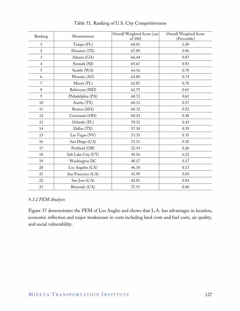
Table 51. Ranking of U.S. City Competitiveness
Ranking Measurement Overall Weighted Score (out of 100)
Overall Weighted Score (Percentile)
1 Tampa (FL) 68.01 1.00 2 Houston (TX) 67.89 0.96 3 Atlanta (GA) 66.44 0.87 4 Newark (NJ) 65.67 0.83 5 Seattle (WA) 64.16 0.78 6 Phoenix (AZ) 63.80 0.74 7 Miami (FL) 62.81 0.70 8 Baltimore (MD) 62.75 0.65 9 Philadelphia (PA) 60.72 0.61
10 Austin (TX) 60.33 0.57 11 Boston (MA) 60.32 0.52 12 Cincinnati (OH) 60.24 0.48 13 Orlando (FL) 59.33 0.43 14 Dallas (TX) 57.30 0.39 15 Las Vegas (NV) 53.35 0.35 16 San Diego (CA) 53.11 0.30 17 Portland (OR) 52.54 0.26 18 Salt Lake City (UT) 49.56 0.22 19 Washington DC 48.17 0.17 20 Los Angeles (CA) 46.30 0.13 21 San Francisco (CA) 43.99 0.09 22 San Jose (CA) 42.81 0.04 23 Riverside (CA) 37.51 0.00
9.3.2 PEM Analysis
Figure 37 demonstrates the PEM of Los Angles and shows that L.A. has advantages in location, economic reflection and major weaknesses in costs including land costs and fuel costs, air quality, and social vulnerability.
M I N E T A T R A N S P O R T A T I O N I N S T I T U T E 127
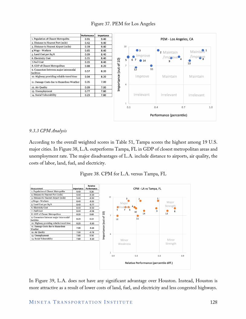
Performance Importance
I. Population of Closest Metropolita 0.91 9.40 PEM - Los Angeles, CA 2. Distance to Nearest Port (mile) 0.42 9.40 3. Distance to Nearest Airport (mile) 0.19 9.40 10
4.Wage-Workers 0.65 8.40 5. Land Cost per Sq ft 0.09 8.40 6. Electricity Cost 0.15 8.40 7.Fue!Coat 0.15 8.40 8. GDP of Closest Metropolitan 0.88 8.20 9. Connectors between major intermodal
0.57 8.20 facilities
.3 •2 1inta·- Mat"'' 1
• • • ,, i's 0 5 6 7 • 14
4 • ~ 9 - 13 0 7 • ... • 11 ::, 12 s.
10. Highway providing reliable travel time 0.04 8.20 QJ 1 .. , .... , ove Maintain Maintain u C
u. Damage Costs due to Hazardous Weather 0.35 7.00 "' t 0 4
12. Air Quality 0.09 7.00 13. Unemployment 0.77 7.80
a. ~
14. Social Vulnerability 0.23 7.80 Irrelevant Irrelevant Irrelevant
0.1 0.4 0.7 1.0
Performance (percentile)
Relative Measurement Importance Performance CPM • LA vs Tampa, Fl 1. Population of Closest Metropolita 9.40 0.26 2. Distance to Nearest Port (mile) 9.40 -0.19 3, Distance to Nearest Airport (mile) 9.40 ·O.SO 4.Wage • Workers 8.40 •0.3S 5. Land Cost per Sq ft 8.40 -0.77 6. Electricity Cost 8.40 ·O.SO 7. Fue1 Coat 8.40 ·O.S8 8. GDP of Closest Metropolitan 8.20 0.69 9. Connectors between major intermodal
8.20 0.22 facilities
10 1 3 2 • • • MdJOr ~
• ... , <:t,
• • s 7 6 • 9 • 8 0 10 14 13 .... • • 0
12 11 -:, 10. Highway providing reliable travel time 8.20 ·0.30 .2. 11. Damage Costs due to Hazardous
7.00 ·0.26 Weather
., u C ..
12. Air Quality 7.00 ·0.78 13. Unemployment 7.80 o.so 14. Social Vulnerability 7.80 ·0.10
t'. 0 C.
E M nor M or
Weakress Strength
I
-0.9 ·0.3 0.3 0.9
Relative Performance (percentile diff.)
Figure 37. PEM for Los Angeles
9.3.3 CPM Analysis
According to the overall weighted scores in Table 51, Tampa scores the highest among 19 U.S. major cities. In Figure 38, L.A. outperforms Tampa, FL in GDP of closest metropolitan areas and unemployment rate. The major disadvantages of L.A. include distance to airports, air quality, the costs of labor, land, fuel, and electricity.
Figure 38. CPM for L.A. versus Tampa, FL
In Figure 39, L.A. does not have any significant advantage over Houston. Instead, Houston is more attractive as a result of lower costs of land, fuel, and electricity and less congested highways.
M I N E T A T R A N S P O R T A T I O N I N S T I T U T E 128
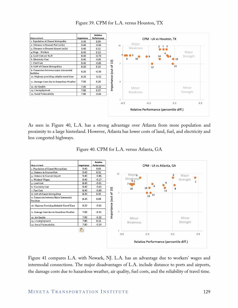
Relative Measurement lmrvvt::r.nce Performance
1. Population of Closest Metropolita 9.40 0.04 CPM - LA VS Houston, TX
2. Distance to Nearest Port (mile) 9.40 -0.04 3. Distance to Nearest Airport (mile) 9.40 0.12
10 Ma,
2 1 3 \A/o-l,n.055 ••• 4.Wage - Workers 8.40 0.13
5. Land Coot per Sq ft 8.40 -0.73
6. Electricity Coot 8.40 -0.81 7. Fuel Coat 8.40 -0.85
8. GDP of Clooest Metropolitan 8.20 0.15
4 Maio• 1••5 • • 9 14 ,8 ,trer,gth
6 10 • • 13 0 .... • • - 11 0 12
9. Connectors between major intermodal 8.20 -0.35
facilities
... :,
.£. 10. Highway providing reliable travel time 8.20 -0.52 QI
u C
u. Damage Costs due to Hazardous Weather 7.00 0.26 "' 4 t:'. 12. Air Quality 7.00 -0.22 13. Unemployment 7.80 0.27 14. Social Vulnerability 7.80 -0.04
0 a. Minor Minor E
Weakress Strrngth
1
-0.9 -0.3 0.3 0.9
Relative Performance (percentile diff.)
Relative
Measurement lmnnrtance Performance CPM - LA vs Atlanta, GA 1. Population of Closest Metropolitan 9.40 0.83
2. DistancetoNearestPort 9.40 0.31
3. Distance to Nearest Airport 9.40 -0.46
4. Workers' Wages 8.40 -0.17
5. Land Cost 8.40 -0.61
6. Electricity Cost 8.40 -0.65
7. Fuel Cost 8.40 -0.69
8. GDP of Clooest Metropolitan 8.20 0.35 9. Connectors between Major IntermOOal
8.20 0.09 Facilities
10 Majo13 2 Major Weaknes~ • Strength • 65 1
7. • 9 4 • • 0 10 14. • 8 .... 13 - •• 0 11 12 ...
:,
.£.
10. Highway Providing Reliable Travel Time 8.20 -0.65 QI u C
~ u. Damage Co.5ts due to Haz:rrd.ous Weather 7.00 -0.31 5 4
a. 12. Air Quality 7.00 -0.22
13. Unemployment 7.80 0.12
14. Social Vulnerability 7.80 -0.24
.§
L Minor Minor
1
Weakness Strength
-0.9 -0.3 0.3 0.9
Relative Performance (percentile diff.)
Figure 39. CPM for L.A. versus Houston, TX
As seen in Figure 40, L.A. has a strong advantage over Atlanta from more population and proximity to a large hinterland. However, Atlanta has lower costs of land, fuel, and electricity and less congested highways.
Figure 40. CPM for L.A. versus Atlanta, GA
Figure 41 compares L.A. with Newark, NJ. L.A. has an advantage due to workers’ wages and intermodal connections. The major disadvantages of L.A. include distance to ports and airports, the damage costs due to hazardous weather, air quality, fuel costs, and the reliability of travel time.
M I N E T A T R A N S P O R T A T I O N I N S T I T U T E 129
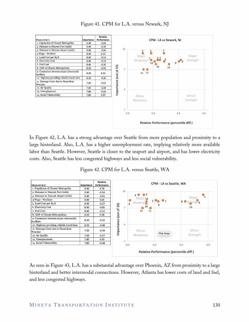
Relative
Measurement Importance Performance CPM - LA vs Newark, NJ 1. Population of Closest Metropolita 9.40 -0.04 2. Distance to Nearest Port (mile) 9.40 -0.35 3. Distance to Nearest Airport (mile) 9.40 -0.54 10
3 2 1 4.Wage - Workers 8.40 0.35 5. Land Cost per Sq ft 8.40 -0.14 6. Electricity Cost 8.40 -0,19 7. Fuel Coat 8.40 -0.35 8. GDP of Closest Metropolitan 8.20 -0,04 9. Connectors between major intermodal
8.20 0.31 facilities
• • • 1; o 7 6 5
8 MaJor
Weakn ..... 9 .. 4 SI rer,gth
10 • • 0 13 14 ... • • .... 0 11 12 ... :,
10. Highway providing reliable travel time 8.20 -0.26 ..2. 11. Damage Costs due to Hazardous
7.00 -0.52 Weather
QJ u C
"' 12. Air Quality 7.00 -0.44 13. Unemployment 7.80 -0.23 14. Social Vulnerability 7.80 0.07
t: 0 a. .§
Mi'lor Minor
Weakress Strength
1
-0.9 -0.3 0.3 0.9
Relative Performance (percentile diff.)
Relative
Measurement Importance Performance CPM - LA vs Seattle, WA
1. Population of Closest Metropolita 9.40 0.78 2. Distance to Nearest Port (mile) 9.40 -0.54
3, Distance to Nearest Airport (mile) 9.40 -0.65 4.Wage - Workers 8.40 0,65
5. Land Cost per Sq ft 8.40 -0,27 6. Electricity Cost 8.40 -0.85
10
3. e2 • M, r 1 10 • • 5 •• •1 8• ii "4 0 6 e,
9 ... 7 .14 • 13 -7, Fuel Coat 8.40 -0.12 0 12 11 .... 8. GDP of Closest Metropolitan 8.20 0.38 9. Connectors between major intermodal
8.20 -0,22 facilities
10. Highway providing reliable travel time 8.20 -0.48
11. Damage Costs due to Hazardous 7,00 -0.39
Weather
12. Air Quality 7.00 -0.57
:,
..2. QJ u C 4 "' t: 0
11/!inor Minor a. .§ Weakness
Plot Area Strength 13, Unemployment 7.80 0.50 14. Social Vulnerability 7.80 -0.48
-0,9 -0,3 0,3 0.9
Relative Performance (percentile diff.)
Figure 41. CPM for L.A. versus Newark, NJ
In Figure 42, L.A. has a strong advantage over Seattle from more population and proximity to a large hinterland. Also, L.A. has a higher unemployment rate, implying relatively more available labor than Seattle. However, Seattle is closer to the seaport and airport, and has lower electricity costs. Also, Seattle has less congested highways and less social vulnerability.
Figure 42. CPM for L.A. versus Seattle, WA
As seen in Figure 43, L.A. has a substantial advantage over Phoenix, AZ from proximity to a large hinterland and better intermodal connections. However, Atlanta has lower costs of land and fuel, and less congested highways.
M I N E T A T R A N S P O R T A T I O N I N S T I T U T E 130
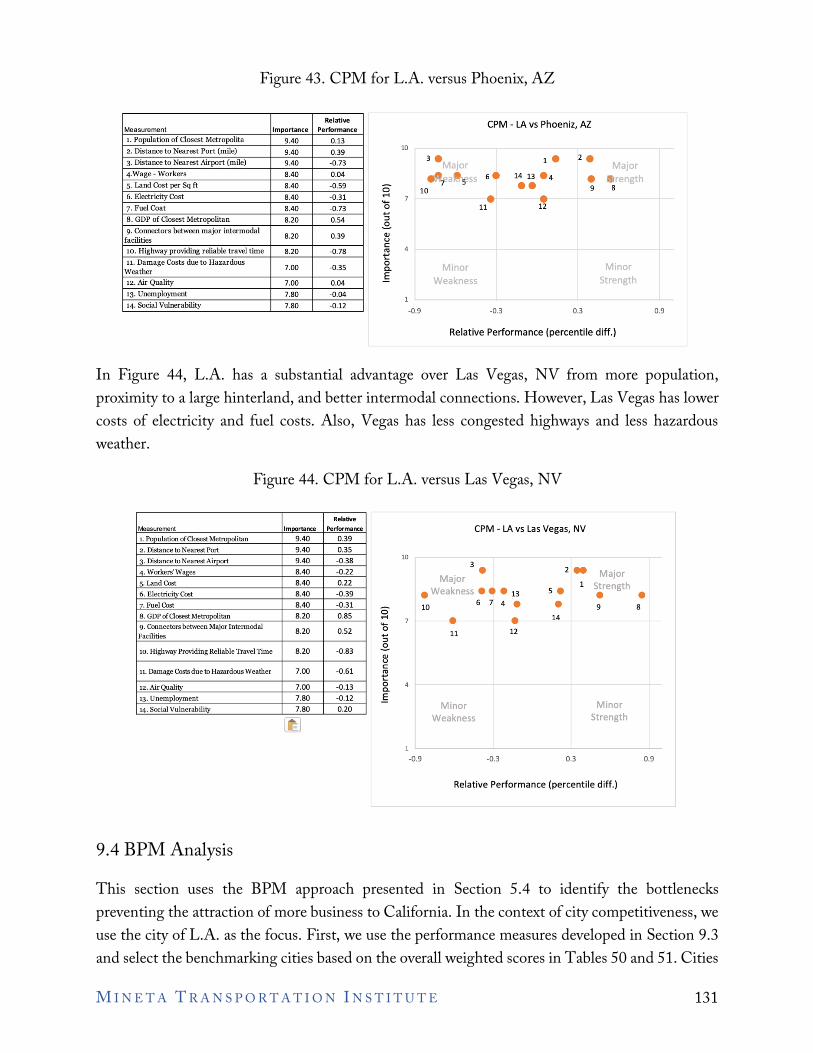
Relative Measurement Importance Performance
t. Population of Closest Metropolita 9.40 0.13 2. Distance to Nearest Port (mile) 9.40 0.39 3. Distance to Nearest Airport (mile) 9.40 -0.73
4.Wage - Workers 8.40 0.04 5. Land Cost per Sq ft 8.40 -0.59 6. EJectricity Cost 8.40 -0.31 7. Fuel Coat 8.40 -0.73
0 ... 0 -8. GDP of Closest Metropolitan 8.20 0.54
9. Connectors between major intermoda1 8.20 0.39 facilities
10. Highway providing reliable travel time 8.20 -0.78 11. Damage Costs due to Hazardous
7.00 -0.35 Weather 12. Air Quality 7.00 0.04
::,
~ Q) u C:
"' t'. 0 C.
1:: 13. Unemployment 7.80 -0.04
14. Social Vulnerability 7.80 -0.12
Relative tv-\easurement lmoortance Performance
1. Population ofOosest Metropolitan 9.40 0.39
2. Distance to Nearest Port 9.40 0.35 3. DistancetoNearest.Airport 9.40 -0.38
4. Workers' Wages 8.40 -0.22
S. Land Cost 8.40 0.22
6. ElectricityCost 8.40 -0.39 7. Fuel Cost 8.40 -0.31
8. GDP of Oosest Metropolitan 8.20 0.85 9. O:mnectors between Major lntermodal
8.20 0.52 Facilities
10. Highway Providing Reliable Travel Time 8.20 -0.83
11. DamageCostsduetoHa1.ardousWeather 7.00 -0.61
12. Air Quality 7.00 -0.13
13. Unemployment 7.80 -0.12
14. Social Vulnerability 7.80 0.20
10
4
1
3.
--, ~5 10
Miror Weak'less
CPM - LA vs Phoeniz, AZ
1 • 2.
6. 14 13 .4 • •• 9
• • 11 12
•,1-·-r
are th 8
Minor Strength
-0.9 -0.3 0.3 0.9
10
Relative Performance (percentile diff.)
CPM - LA vs Las Vegas, NV
3.
Major .. Major
• Weakness • • • 13 5. Strength • 10
-0.9
• 11
Minor Weakness
6 7 4 •
-0.3
• 12
• 14
0.3
9
Minor Strength
Relative Performance (percentile diff.)
• 8
0.9
Figure 43. CPM for L.A. versus Phoenix, AZ
In Figure 44, L.A. has a substantial advantage over Las Vegas, NV from more population, proximity to a large hinterland, and better intermodal connections. However, Las Vegas has lower costs of electricity and fuel costs. Also, Vegas has less congested highways and less hazardous weather.
Figure 44. CPM for L.A. versus Las Vegas, NV
9.4 BPM Analysis This section uses the BPM approach presented in Section 5.4 to identify the bottlenecks preventing the attraction of more business to California. In the context of city competitiveness, we use the city of L.A. as the focus. First, we use the performance measures developed in Section 9.3 and select the benchmarking cities based on the overall weighted scores in Tables 50 and 51. Cities
M I N E T A T R A N S P O R T A T I O N I N S T I T U T E 131
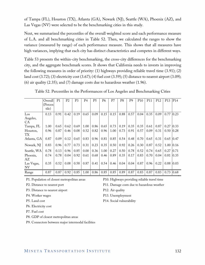
of Tampa (FL), Houston (TX), Atlanta (GA), Newark (NJ), Seattle (WA), Phoenix (AZ), and Las Vegas (NV) were selected to be the benchmarking cities in this study. Next, we summarized the percentiles of the overall weighted score and each performance measure of L.A. and all benchmarking cities in Table 52. Then, we calculated the ranges to show the variance (measured by range) of each performance measure. This shows that all measures have high variances, implying that each city has distinct characteristics and competes in different ways. Table 53 presents the within-city benchmarking, the cross-city differences for the benchmarking city, and the aggregate benchmark scores. It shows that California needs to invests in improving the following measures in order of priority: (1) highways providing reliable travel time (3.91); (2) land cost (3.72); (3) electricity cost (3.67); (4) fuel cost (3.59); (5) distance to nearest airport (3.09); (6) air quality (2.35); and (7) damage costs due to hazardous weather (1.96).
Table 52. Percentiles in the Performances of Los Angeles and Benchmarking Cities
Overall (Percen
tile)
P1 P2 P3 P4 P5 P6 P7 P8 P9 P10 P11 P12 P13 P14
Los Angeles, CA
0.13 0.91 0.42 0.19 0.65 0.09 0.15 0.15 0.88 0.57 0.04 0.35 0.09 0.77 0.23
Tampa, FL 1.00 0.65 0.62 0.69 1.00 0.86 0.65 0.73 0.19 0.35 0.35 0.61 0.87 0.27 0.33 Houston, TX
0.96 0.87 0.46 0.08 0.52 0.82 0.96 1.00 0.73 0.91 0.57 0.09 0.31 0.50 0.28
Atlanta, GA 0.87 0.09 0.12 0.65 0.83 0.96 0.81 0.85 0.54 0.48 0.70 0.65 0.31 0.65 0.47 Newark, NJ 0.83 0.96 0.77 0.73 0.31 0.23 0.35 0.50 0.92 0.26 0.30 0.87 0.52 1.00 0.16 Seattle, WA 0.78 0.13 0.96 0.85 0.00 0.36 1.00 0.27 0.50 0.78 0.52 0.74 0.65 0.27 0.71 Phoenix, AZ
0.74 0.78 0.04 0.92 0.61 0.68 0.46 0.89 0.35 0.17 0.83 0.70 0.04 0.81 0.35
Las Vegas, NV
0.35 0.52 0.08 0.58 0.87 0.41 0.54 0.46 0.04 0.04 0.87 0.96 0.22 0.88 0.03
Range 0.87 0.87 0.92 0.85 1.00 0.86 0.85 0.85 0.89 0.87 0.83 0.87 0.83 0.73 0.68 P1. Population of closest metropolitan areas P10. Highways providing reliable travel time P2. Distance to nearest port P11. Damage costs due to hazardous weather P3. Distance to nearest airport P12. Air quality P4. Worker wages P13. Unemployment P5. Land cost P14. Social vulnerability P6. Electricity cost P7. Fuel cost P8. GDP of closest metropolitan areas P9. Connectors between major intermodal facilities
M I N E T A T R A N S P O R T A T I O N I N S T I T U T E 132
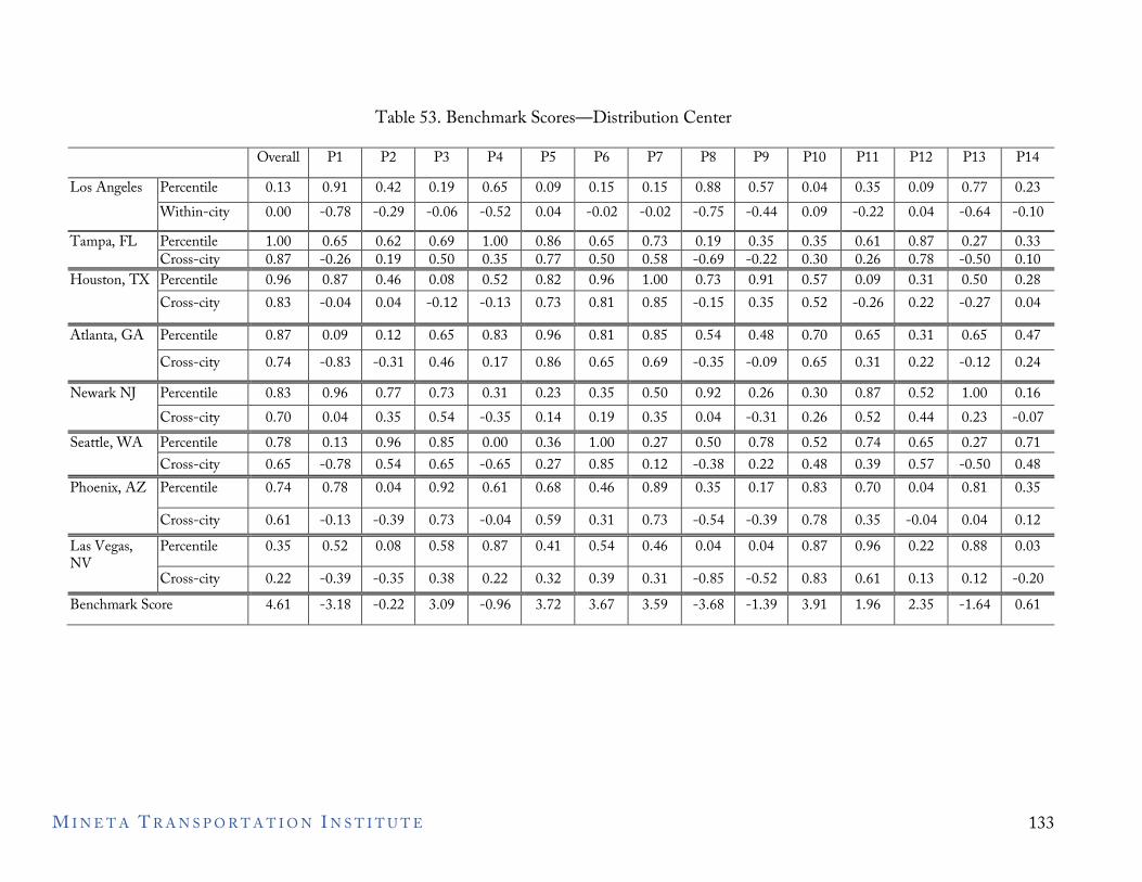
I I I I I I I I I I I I I I
Table 53. Benchmark Scores—Distribution Center
Overall P1 P2 P3 P4 P5 P6 P7 P8 P9 P10 P11 P12 P13 P14 Los Angeles Percentile 0.13 0.91 0.42 0.19 0.65 0.09 0.15 0.15 0.88 0.57 0.04 0.35 0.09 0.77 0.23
Within-city 0.00 -0.78 -0.29 -0.06 -0.52 0.04 -0.02 -0.02 -0.75 -0.44 0.09 -0.22 0.04 -0.64 -0.10 Tampa, FL Percentile 1.00 0.65 0.62 0.69 1.00 0.86 0.65 0.73 0.19 0.35 0.35 0.61 0.87 0.27 0.33
Cross-city 0.87 -0.26 0.19 0.50 0.35 0.77 0.50 0.58 -0.69 -0.22 0.30 0.26 0.78 -0.50 0.10 Houston, TX Percentile 0.96 0.87 0.46 0.08 0.52 0.82 0.96 1.00 0.73 0.91 0.57 0.09 0.31 0.50 0.28
Cross-city 0.83 -0.04 0.04 -0.12 -0.13 0.73 0.81 0.85 -0.15 0.35 0.52 -0.26 0.22 -0.27 0.04
Atlanta, GA Percentile 0.87 0.09 0.12 0.65 0.83 0.96 0.81 0.85 0.54 0.48 0.70 0.65 0.31 0.65 0.47 Cross-city 0.74 -0.83 -0.31 0.46 0.17 0.86 0.65 0.69 -0.35 -0.09 0.65 0.31 0.22 -0.12 0.24
Newark NJ Percentile 0.83 0.96 0.77 0.73 0.31 0.23 0.35 0.50 0.92 0.26 0.30 0.87 0.52 1.00 0.16 Cross-city 0.70 0.04 0.35 0.54 -0.35 0.14 0.19 0.35 0.04 -0.31 0.26 0.52 0.44 0.23 -0.07
Seattle, WA Percentile 0.78 0.13 0.96 0.85 0.00 0.36 1.00 0.27 0.50 0.78 0.52 0.74 0.65 0.27 0.71 Cross-city 0.65 -0.78 0.54 0.65 -0.65 0.27 0.85 0.12 -0.38 0.22 0.48 0.39 0.57 -0.50 0.48
Phoenix, AZ Percentile 0.74 0.78 0.04 0.92 0.61 0.68 0.46 0.89 0.35 0.17 0.83 0.70 0.04 0.81 0.35
Cross-city 0.61 -0.13 -0.39 0.73 -0.04 0.59 0.31 0.73 -0.54 -0.39 0.78 0.35 -0.04 0.04 0.12 Las Vegas, NV
Percentile 0.35 0.52 0.08 0.58 0.87 0.41 0.54 0.46 0.04 0.04 0.87 0.96 0.22 0.88 0.03
Cross-city 0.22 -0.39 -0.35 0.38 0.22 0.32 0.39 0.31 -0.85 -0.52 0.83 0.61 0.13 0.12 -0.20 Benchmark Score 4.61 -3.18 -0.22 3.09 -0.96 3.72 3.67 3.59 -3.68 -1.39 3.91 1.96 2.35 -1.64 0.61
M I N E T A T R A N S P O R T A T I O N I N S T I T U T E 133
9.5 Comments from Interviews The above quantitative analysis was complemented with a qualitative discussion of interviewee responses to open-ended questions. For example, experts were asked about data and measures of competitiveness in the locations of distribution centers, the current and future state of California’s competitiveness in the locations of distribution centers, and related issues of environmental impact, sustainability, and resilience. 9
9.5.1 Data and measures
Several experts mentioned that availability of labor, operating costs, access to infrastructure, state subsidies, proximity to ports and airports, political stability, trade lane flows, and the weather are the key factors that firms consider in location selection. Experts agreed that the performance measures proposed in Table 48 are appropriate to represent firms’ decisions when choosing locations of distribution centers. In addition to the measures listed in Table 48, experts mentioned the following measures that could be used for this study:
• Location factors: availability of industrial zone, distance to fuel source, distance to freeways, locations of other branches in the company and locations of Amazon’s fulfillment centers.
• Cost factors: insurance costs and cost of regulation. • Environmental factors: conditions of the road, CO2 emissions and renewal energy, and cost
of environmental regulation.
9.5.2 Current state of California freight competitiveness
Experts mentioned that California’s potential competitors include the Pacific Northwest (primarily Washington and Oregon), the Chicago Area (Joliet and around), the NJ corridor (turnpike from NJ to PA), Texas (Dallas for domestic supply chain and Houston for import), and the Southeast (mainly Savannah but Charleston is pushing further). In addition, Ohio and Kentucky have been attractive for e-commerce operations.
Experts observed that some investments had been made in California in the past years:
• More eco-friendly types of warehouses with skylights, LED lighting, solar panel installation.
• New distribution centers in Northern California (Patterson) and Southern California (Mira Loma, San Bernardino).
• Trying to electrify the ports—converting diesel equipment to electric. • California invested billion dollars on the bridge at Port of Long Beach to accommodate
larger cargo ships.
M I N E T A T R A N S P O R T A T I O N I N S T I T U T E 134
Experts also reported several bottlenecks to keeping business in California. First, space availability is an issue in California. The industrial zone is scarce, and the number of dock doors in the distribution centers is always a problem. The supply of the industrial zone is shrinking, but the demand is growing. Rental rates continue to go up 3 or 4% a year, even amid COVID. From 2020 to 2025, the projected rent growth in L.A. County is 41%. Firms are leaving California and moving to Phoenix and Vegas. Second, there is a significant lack of qualified labor in California. People think of warehouses as working at a fast-food places, where people are making minimum wage. However, jobs in distribution centers are relatively well-paying jobs because these facilities are becoming significantly more high-tech-oriented. Third, labor disputes cause delays to the distribution system. Union labors at ports have extended turn-around times. Fourth, congested freeways are a bottleneck in California. The increased population and more cars on the road cause longer transit time. Fifth, LAX and the Ports of L.A./L.B. cause delays because of flight availability and shipments being put on hold. The dray pool is getting tighter. Airports (LAX) are the key bottleneck in California. Lastly, labor costs, transportation, fuel, land, and electricity are too high in California. Therefore, regulations on emission cause overburdens on trucks.
9.5.3 The future of California freight competitiveness
To make California more competitive, experts have the following suggestions. First, California should lower taxes and regulations. The regulations such as environmental regulations, OSHA (Occupational Safety and Health Administration) regulations and Prop 15 have increased the burden on the warehousing industry. California could consider an indirect source rule of emissions, e.g., tax proposed on warehouses for diesel trucks, or mitigate by greening warehouse operations. State subsidies in labor costs, and taxes can help reduce the costs of doing business in California. Second, California should reduce restrictions on industrial zoning, making industrial warehouses more available. Third, California should modernize infrastructure at the ports and automate the inventory system. There will be more automated vehicles that drive themselves in the future. Fourth, California needs to be more competitive in the intermodal sector, such as port-rail connections. Lastly, California needs to educate the workforce. More education and training are needed to help the workforce develop the skill sets needed to operate in high-tech facilities.
M I N E T A T R A N S P O R T A T I O N I N S T I T U T E 135
9.6 Distribution Center Performance with respect to the Environment, Sustainability, and Resilience
Experts indicated that California is rather resilient in facing disasters, outages, and accidents. Most companies have contingency plans that allow them to consider potential disasters and prepare for them. For example, some firms have other distribution centers that would take extra inventory in the case of an accident. The COVID pandemic showed that distribution centers are well prepared because many third-party logistics providers already had a business recovery plan. Experts observed that California has made the following investments in sustainability:
• CO2 measurement: Firms need to align the infrastructure with the future regulations to make warehouse users accountable for CO2 emission.
• Electric yard goats: Goats were used in Seattle in the past to clean up the grass and bushes around warehouses.
• Solar panel deployment.
Experts argued that the environmental regulations have added burdens to distribution centers. They mentioned that the Carbon memorandum is one of the interesting things they have seen in the last few years. The South Coast Air Quality Management District (AQMD) is a very aggressive regulator of emissions and overly burdensome on trucks. Experts propose several suggestions to enhance sustainability and resilience. First, rooftop solar panels can offset the relative impact of the demand of electricity in these facilities. For example, a firm can put up a 1020 thirty hundred kW solar rooftop system and essentially offset the electrical demand for the building. Second, green building design should be advocated for more. For example, a building with higher insulation on the roof decks and a better glazing windows system is more efficient. In addition, a building with white reflective roofs does not collect heat and saves more electricity. Third, California needs more electric charging stations in warehouse distribution centers. Trucks are idle at the docks when they are loading and unloading. Electrical connections can be available at the docks for trucks to plug into. More electric forklifts should be used to replace propane forklifts. Carl Moyer Grants can be used to buy zero-emissions trucks.
9.7 Conclusion 9.7.1 Findings
In the past 15 years, the demographic trends show that large metropolitan areas, such as L.A., are losing shares in terms of populations and employment to emerging metropolitan areas like Riverside-San Bernardino-Ontario, Dallas, Houston, Seattle, Atlanta, and Phoenix. Lower costs
M I N E T A T R A N S P O R T A T I O N I N S T I T U T E 136
of rent and wages and the surge of demand for e-commerce are the main contributors to this trend. Thus, while the GDP growth in San Francisco and San Jose is mainly driven by higher productivity, that in Dallas, Houston, and Atlanta is more driven by move-in populations. The PEM and CPM approaches identify the strengths, the weaknesses, and the competitive position of LA. On the one hand, L.A. has substantial competitive advantages in location and economic reflection. L.A. is located in a metropolitan area with a large economy and population close to two major ports and airports. On the other hand, L.A. has major weaknesses due to the air quality, social vulnerability, and the land, fuel, and labor costs. Based on the overall weighted scores, the top five cities attractive to business in the U.S. are (1) Tampa, FL, (2) Houston, TX, (3) Atlanta, GA, (4) Newark NJ, and (5) Seattle, WA, which are considered potential competitors of California cities. In addition, experts mentioned that California is competing with Phoenix, AZ and Las Vegas, NV. For the BPM analysis, it is suggested that the state should prioritize investment in highways, which can provide reliable travel time and in lowering the costs of land, electricity, and fuel. When considering the current state of California city competitiveness, experts indicated that lack of industrial zones and qualified labor coupled with excessive operations costs are bottlenecks for keeping businesses in California. Experts proposed that California may increase competitiveness by reducing taxes, subsidizing labor costs, and releasing regulations on the environment and industrial zones. In addition, the state needs to invest in modernizing infrastructure at the ports and automating inventory systems.
9.7.2 Suggestions
The costly and scarce industrial zone in the Los Angeles-Long Beach-Anaheim metropolitan areas and booming e-commerce development has increased the attractiveness of the Inland Empire and Central Valley. California needs to invest in providing better intermodal transport service between seaports, airports, freight rails, and highways. Given congestion on urban interstates and poor highway travel time reliability in California, the state should consider investing in inland ports, transporting goods by rail directly from seaports to processing facilities inland, in the Inland Empire and Central Valley.
9.7.3 Workforce Development Plan
While workforce entities may not control land costs and availability, they can upskill and improve soft and technical skills leading to efficiency and quality assurance. As this sector already has moved toward new, more efficient, and safer inventory and tracking technologies, they will soon go beyond testing alternate forms of connecting the warehouse with their markets via unmanned vehicles (UV) such as flying taxis and drones.
M I N E T A T R A N S P O R T A T I O N I N S T I T U T E 137
The workforce will need to be trained, or retrained, to build, maintain, operate, manage, and even learn how to sell the use of these robots and UVs to new and existing middle and end user markets. These opportunities will be open to those with multiple levels of education and to a huge generation of young, tech savvy people ready to or recently entering the job market. Given the overall labor shortage, these technological advances and use of terminology such as ‘logistics, robotics,’ etc. could excite the younger, more tech savvy workforce to reconsider opportunities available. A proper workforce development plan will engage training institutions to ensure they have developed appropriate curriculum and tools that are technologically advanced. This would involve meeting with business to help develop both what and how to teach, to meet industry needs. The logistics industry is ripe for apprenticeship models that provide earn-and-learn opportunities promoted to a diverse population through channels ‘where they are’, potentially via social media and networking. Public-private partnerships with major players such as Amazon and Walmart already exist and should be leveraged to ensure workforce planning and execution meets their needs and are visualized for the future.
M I N E T A T R A N S P O R T A T I O N I N S T I T U T E 138
10. Public Policy Recent state and federal policy initiatives have the potential to impact California’s freight industry. This section looks at three plans that have notable potential impact: the 2020 California Freight Mobility Plan; the 2018 California State Rail Plan; and the U.S. Senate 2021 Infrastructure Investment and Jobs Act. The proposed investments would be a combination of public and private funding and would represent a significant increase in spending. While the U.S. federal government continues to debate major national infrastructure spending bills, California has committed funds to congested trade and commuter corridor improvements through SB1, the Road Repair and Accountability Act of 2017.
10.1 2020 California Freight Mobility Plan The 2020 California Freight Mobility Plan (CFPM) was developed by Caltrans to “provide a long-term vision for California’s freight future” (2020 CFMP). California aims to achieve a multimodal freight network that represents an example to the world and is innovative, competitive, efficient, reliable, modern, and sustainable. The plan proposes four themes for the state’s most critical investments:
• improving port access reliability; • border efficiency; • inter- and intra-state freight movement and resiliency; and • and sustainability and innovations.
The 2020 CFMP discusses California’s cost differences in trucking, railroad, ocean shipping, air cargo, land, energy, and utility. The findings show that California has relatively high costs in most categories. Motor carriers within California are concerned about highway and facility congestion that reduces driver productivity, vehicle productivity, effective capacity, and increases port drayage costs. Regarding distribution center operating costs among 25 cities in the U.S., California locations had the highest annual combined costs, except for a few locations in the Northeast and Idaho. The 2020 CFMP also reports that several freight industry experts perceive an “anti-business” attitude in California according to its environmental regulations, high taxes and fees, and opposition to facility development. However, they believe California is attracting business activity tied to specific state industry clusters, such as the high-tech or green energy sectors (2020 CFMP, 41). The 2020 California Freight Mobility Plan presents numerous goals, some of which are particularly relevant to seaports and airports. The following goals are selected from that broader list:
• Goal 1: Multimodal Mobility • “Identify causes and solutions to freight bottlenecks.”
M I N E T A T R A N S P O R T A T I O N I N S T I T U T E 139
• “Invest strategically to optimize system performance.” • “Develop, manage, and operate an efficient, integrated freight system.” • Goal 2: Economic Prosperity • “Promote economic development by investing in freight infrastructure projects and
operational improvements.” • “Promote freight projects that enhance economic activity, freight mobility, unique
capabilities, reliability, system resiliency, and global competitiveness.” • “Promote the State’s competitive logistics advantages.” • Goal 5: Safety and Resilience • “Utilize technology to provide for the resilience and security of the freight transportation
system.” • “Work with State and Federal homeland security partners to ensure that future
transportation design decisions near sea, air, and land ports of entry account future space requirements for cargo screening facilities.”
• “Ensure consistent and effective safety and security requirements at all California ports.” • “Identify alternate freight routes to maintain freight movement at times of disruption by
disaster.” • “Incorporate resilience strategies contained in port plans prepared pursuant to coastal
commission guidelines.” • Goal 7: Connectivity and Accessibility • “Promote innovative technologies and practices utilizing real-time information to move
freight on all modes more efficiently.” • “Utilize inland port facility, short-haul rail shuttle, and inland seaports to lessen impacts
on nearby communities.”
This project, which evaluates the state’s competitive position, identifies the freight bottlenecks and proposes priorities for investments, directly contributes to achieving these goals. With respect to seaports specifically, the 2020 CFMP indicated that some bottlenecks exist in each region of California. In the San Francisco Bay Area, the Port of Oakland faces some landside challenges and has been affected by a sudden surge in larger post-Panama expansion ships. The Port of Oakland contributed 29% of the pollution to the West Oakland community, including emissions, noise, and light from port operations. However, the air quality has been significantly improved through the Port of Oakland’s Seaport Air Quality 2020 and Beyond Plan. Diesel particulate matter has been reduced by 81%. Truck diesel emissions and ship emissions have dropped 98% and 78%, respectively, over the past decades (CFMP 2020, 271). The Port of Oakland also identified a significant constraint, at-grade railroad crossings in the Port, leading to significant truck queues. The Global Opportunities at the Port of Oakland (GoPort) project, which proposed grade separation and roadway reconfiguration, would eliminate the at-grade crossing, and improve operations (CFMP 2020, 273).
M I N E T A T R A N S P O R T A T I O N I N S T I T U T E 140
In Southern California, the 2020 CFMP indicated that the share of total inland point intermodal (IPI) (inbound and outbound) containers through the Ports of Los Angeles and Long Beach had dropped significantly from 43% in 2006 to 30% in 2018 (2020 CFMP, 35). While many factors can be attributed to faster growth on the Atlantic and Gulf Coasts, two factors are specific to POLA/POLB. First, the "clean truck" requirements led to increased costs at Southern California ports. The Pier Pass/Off-Peak fees and drayage costs increased due to port and highway congestion. Second, firms have concerns over the West Coast’s labor relations stability, after the lengthy 2014– 2015 dispute and accompanying shipping disruption. With respect to airports specifically, the 2020 CFMP indicates that direct competition among airports for air cargo business is mainly regional. Oakland (OAK) and San Francisco (SFO) compete for Bay Area air cargo, with OAK prevailing in domestic and SFO in international shipping. FedEx has a major capacity at OAK. LAX and Ontario (ONT) compete for air cargo in Southern California, with LAX having the dominant share. UPS has a primary facility at ONT (2020 CFMP, 37). Also, the 2020 CFMP points out that air cargo is increasingly dominated by integrated carriers such as FedEx, UPS, and DHL. As a result, California airports are competing for the business of the integrated carriers rather than for the underlying customer choices. As we consider the results of our analysis of California’s highway system, it is clear that California has some clear strengths and weaknesses, representing a clear opportunity to maintain and advance its favorable position in the country and the world. Among the goals and objectives of this plan, there is a call for support and promotion of investments to enhance the state’s competitiveness and identify and propose solutions to roadway bottlenecks. These seem appropriate goals given the main results from this section. According to our main results from this section, addressing the congestion in urban interstates and improving the percentage of highways providing reliable travel time seems to represent a critical bottleneck in the highway freight system, but also an opportunity that can be seized with the appropriate investments. Considering the highway freight experts’ opinions, one of those investments could be to develop freight-exclusive lanes and sectors that connect the major intermodal facilities and the main freight corridors in the country. Another investment that could directly impact these performance measures would be to invest in the repair and maintenance of highways, bridges, and railways. Together, these investments could substantially improve California’s competitive standing in terms of highway freight. In addition, the 2020 CFMP indicates the critical role of the industrial warehouses and distribution centers in Southern California. They are connection points for all modes of transportation, and provide necessary services to stock inventory, trans-load, and interchange transitional cargo, fulfill orders, perform value-added services such as just-in-time delivery, among others. Moreover, they are clustered along key goods movement highway corridors including:
M I N E T A T R A N S P O R T A T I O N I N S T I T U T E 141
• The I-405, which provides access to clusters of air cargo facilities where sorting and consolidation/de-consolidation activities occur near LAX.
• The I-710, which provides access to logistics service providers, truck terminals, and trans-load facilities serving the goods movement industry near the San Pedro Bay Ports, as well as provides connections to the warehouse concentrations in downtown Los Angeles and east Los Angeles, and intermodal rail yards.
• The I-5 providing access to warehouse clusters in the Gateway Cities sub-region and areas in northern Orange County.
• The East-west corridors, including SR 60 and I-10, provide access to major warehouse clusters in the San Gabriel Valley and the Inland Empire.
The CFMP presents numerous goals that relate explicitly to freight rail:
• Goal 1: Multimodal Mobility • “Identify causes and solutions to Freight Rail Network Improvements bottlenecks” • “Identify freight rail network operational improvements and model shift options” • Goal 7: Connectivity and Accessibility • “Utilize inland port facility, short-haul rail shuttle, and inland seaports to lessen impacts
on nearby communities”
In addition to the bottlenecks identified above, the report suggests that California’s rail infrastructure is in good shape, with the majority of rail infrastructure able to accommodate double-stacking and higher-weight railcars. This is likely due to the private ownership and investment schedules of most California railroads. Other general freight system improvements discussed in the plan—such as optimizing system performance, integrating the freight system, improving workforce availability and training, and reducing emissions—could also benefit freight rail. Where freight rail proposals are identified— such as inland port facilities and automated rail yards—appropriate realism regarding the limitations with respect to cost and planning complexity is required. For example, challenges around designing and developing automated Terminal Operation Systems for rail yards mean that rail has been slower to implement automated facilities than the warehousing sector. The report presents detailed opportunities for investment in freight rail in section 6.7 with respect to each region (Northern California, Central Sierra, Bay Area, Central Valley, Central Coast, Los Angeles and Inland Empire, and San Diego Border).
10.2 2018 California State Rail Plan In the 2018 California State Rail Plan (Caltrans 2018), six areas of opportunity were identified for freight rail in California:
• Trade corridor improvements.
M I N E T A T R A N S P O R T A T I O N I N S T I T U T E 142
• Economic development and short lines. • Grade-crossing improvement needs throughout the state. • Additional terminal and yard capacity. • Short-haul rail improvements. • Advancement of zero and near-zero emissions technologies.
The corridor-based approach prioritizes short-term (2022) investments to addressing trade corridor bottlenecks. In the medium term (2027), the state plan recommends investment in dedicated freight capacity to improve primary trade corridors, as well as state investment in passenger rail networks in shared corridors that provides capacity benefits for freight rail. In the long term (2040) additional investments are recommended in the integration of multiple modes and inter-modal sites that provide benefits across interregional investment corridors (Caltrans 2018). With respect to bottlenecks, the report references eight key “chokepoints”:
• BNSF San Bernardino–Los Angeles: San Bernardino via Fullerton and Riverside • BNSF Cajon: Barstow to Keenbrook • UPRR Sunset Route: Yuma Subdivision • UPRR Alhambra and Los Angeles • UPRR Martinez: Oakland to Martinez • Southern Oakland Route: Oakland to Niles Junction • BNSF Main Line Stockton to Bakersfield: San Joaquin Corridor • UPRR Roseville to Reno over Donner Pass
10.3 2021 Infrastructure and American Jobs Act This section looks at proposed funding in the U.S. Senate’s 2021 Infrastructure and American Jobs Act11 dedicated to seaports, airports, highways, and rail over the next five years. There are no dedicated funds for distribution centers and warehouses, although there may be elements of the bill that benefit this segment. The bill dedicates $17 billion in inland waterways, coastal ports, land ports of entry, and ferries. However, the majority of this—over $10 billion—is assigned to US Army Corps of Engineers and US Coast Guard infrastructure priorities, including repairing natural disaster damage. Some of this funding will indirectly benefit seaports and related waterways. Of the remaining funding, around $3.5 billion is dedicated to sea and waterway ports: $2.25 billion is allocated to the Department of Transportation’s Port Infrastructure Development Program, $400 million is
11 At the time of writing, the Senate’s Infrastructure Investment and Jobs Act is the latest version of an infrastructure bill originally proposed by the Biden administration. The bill has yet to be approved by the House or President Biden.
M I N E T A T R A N S P O R T A T I O N I N S T I T U T E 143
assigned to reduction of truck emissions at ports, and $912 million is allocated to ferry boat and terminal construction. Another $3.85 billion is allocated to “Land Ports of Entry Modernization and Construction,” which has more relevance to trucking freight. As the Ports of Los Angeles, Long Beach, and Oakland are the first, third, and tenth largest ports in terms of TEUs— accounting for 36.6% of total TEUs (Burnson 2021)—it is likely that they will receive a significant share of this funding. $25 billion is dedicated to U.S. airports, including $20 billion for airside and terminal projects, to develop runways, taxiways, terminals, and multimodal facilities. Another $5 billion is allocated to air traffic control infrastructure investments (U.S. Chamber of Commerce 2021). Central to the bill is $110 billion in new investment in interstate highways, to modernize 20,000 miles of highways, roads, and main streets, rebuild bridges in disrepairs, and provide critical linkages to our communities. Specifically, these include $36.7 billion for bridge grant programs, $10.2 billion for regional and local surface transportation projects, $5 billion for multi-modal and multi-jurisdictional projects, and $1 billion for culvert removal, replacement, and restoration (U.S. Chamber of Commerce 2021). There is also a further $10.5 billion in new funding to support safety improvements and research. Also notable is $3.85 billion allocated to “Land Ports of Entry Modernization and Construction,” which will alleviate bottlenecks at ports of entry for trucking freight (U.S. Chamber of Commerce 2021). To the extent that these investments are expected to improve conditions for freight flows in California’s highway system by reducing congestion and improving reliable travel times, the Infrastructure and American Jobs Act has the potential to improve the California’s competitive position in the country and the world. $66 billion is dedicated to passenger and freight rail. This funding is primarily to support passenger rail. Unlike passenger rail, federal support for freight railroads is already limited, and policy makers are of the opinion that freight rail functions well with private investment. However, there is money for capital investments, such as $5 billion for rail infrastructure and safety improvements, and $3 billion for railroad crossing elimination, that could benefit freight rail directly. In addition, improvements to the passenger rail network and infrastructure could indirectly benefit freight rail, especially in congested corridors where the two compete for track. Another benefit could come from investments to reduce congestion at ports as well as neighboring highway and intermodal sites. While there are no dedicated funds for warehousing and distribution centers, this segment will benefit indirectly from improvements to the ports, highway, and intermodal systems in particular. Also funds provided for broadband and the power grid could propel the facilities to greater business efficiencies and cost savings.
M I N E T A T R A N S P O R T A T I O N I N S T I T U T E 144
11. Summary and Conclusions 11.1 Overall Competitiveness Scores This section concludes this study by generating the overall competitiveness scores for California and competing states. We use the weights of each freight sector generated in Section 4 and the overall performance percentiles of the leading entity (seaport, airport, city, or state) in Sections 5, 6, 7, 8, and 9 to generate the overall competitiveness scores. In Section 4, we asked industry experts to evaluate the contributions of five freight sectors to the supply chain using a 10-point scale. Then we converted the contribution scores to the contribution weights, which add up to 100 percent, as shown in Table 4. In Sections 5, 6, 7, 8, and 9, we analyzed the performances of the five freight sectors, including seaports, airports, highways, freight rails, and distribution centers, and generated the overall weighted performances of California and competing states. Given that one state may have more than one seaport, airport, and city, we used the one with the highest overall weighted performance to represent that state. In addition, we choose only the states with all the five freight sectors, so that we can directly compare their overall competitiveness scores. As a result, the five competing states chosen were Texas, Georgia, Washington, New York/New Jersey, and Florida. Table 54 reports the overall weighted scores of the five freight sectors for California and the competing states. The overall competitiveness scores are generated by the product of the weights and the overall weighted score percentiles on each freight sector. It shows that the top three competitors to California (overall competitive score of 0.54) are New York and New Jersey (0.82), Texas (0.81), and Georgia (0.75). The top competitors are New York and New Jersey. The GDP of the New York-Newark-Jersey City metropolitan areas is similar to that of Southern California. Their seaports and airports and California’s are both ranked among the top in the U.S. but New York and New Jersey outperform California in highways and distribution centers. The primary advantages for New York and New Jersey over California are more reliable travel time and lower costs of doing business than California. The next highest competitor is Texas, which outperforms California in highways, rails, and distribution centers. While California owns very competitive seaports and airports, Texas is a good rival which owns a top-performance airport (DFW) and freight rail system. Moreover, the costs of doing business in Texas are much lower than in California, attracting many firms to relocate their headquarters and operations centers. The third top competitor is Georgia. Georgia is an emerging state and owns a growing seaport (Savannah), airport (ATL), and cities (Atlanta). As mentioned in Section 5.1, the Port of
M I N E T A T R A N S P O R T A T I O N I N S T I T U T E 145
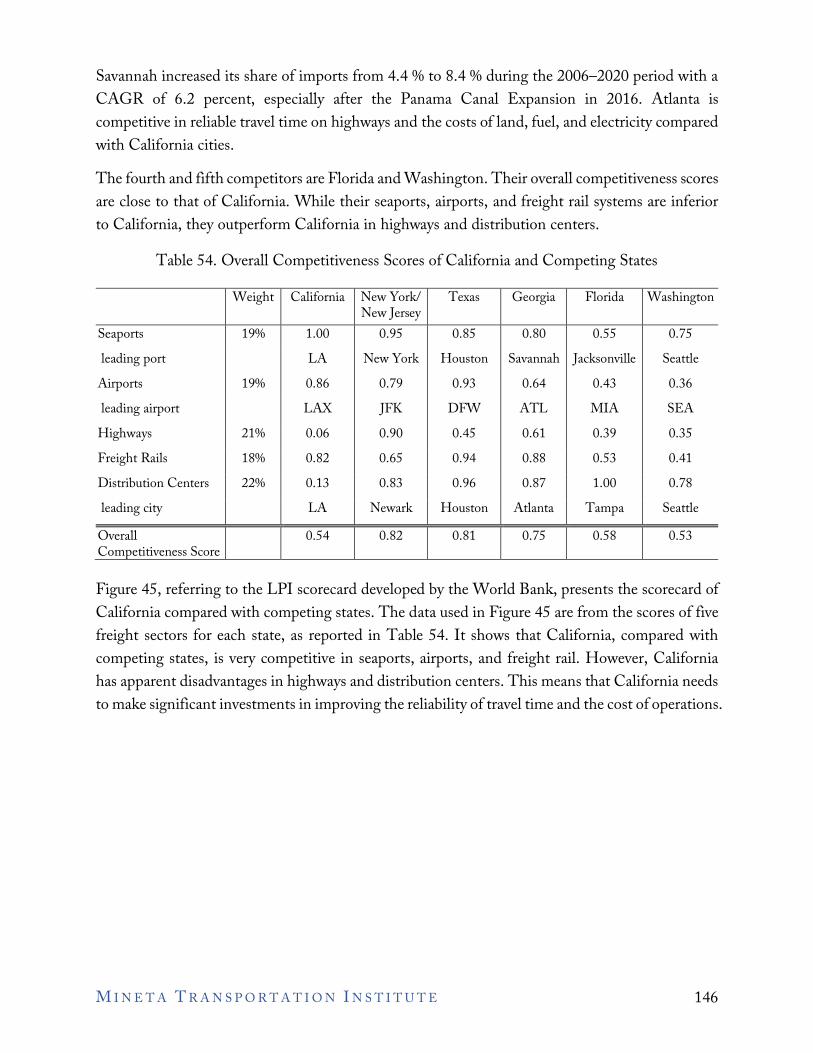
M I N E T A T R A N S P O R T A T I O N I N S T I T U T E 146
Savannah increased its share of imports from 4.4 % to 8.4 % during the 2006–2020 period with a CAGR of 6.2 percent, especially after the Panama Canal Expansion in 2016. Atlanta is competitive in reliable travel time on highways and the costs of land, fuel, and electricity compared with California cities. The fourth and fifth competitors are Florida and Washington. Their overall competitiveness scores are close to that of California. While their seaports, airports, and freight rail systems are inferior to California, they outperform California in highways and distribution centers.
Table 54. Overall Competitiveness Scores of California and Competing States
Weight California New York/ New Jersey
Texas Georgia Florida Washington
Seaports 19% 1.00 0.95 0.85 0.80 0.55 0.75 leading port
LA New York Houston Savannah Jacksonville Seattle
Airports 19% 0.86 0.79 0.93 0.64 0.43 0.36 leading airport
LAX JFK DFW ATL MIA SEA
Highways 21% 0.06 0.90 0.45 0.61 0.39 0.35 Freight Rails 18% 0.82 0.65 0.94 0.88 0.53 0.41 Distribution Centers 22% 0.13 0.83 0.96 0.87 1.00 0.78 leading city LA Newark Houston Atlanta Tampa Seattle Overall Competitiveness Score
0.54 0.82 0.81 0.75 0.58 0.53
Figure 45, referring to the LPI scorecard developed by the World Bank, presents the scorecard of California compared with competing states. The data used in Figure 45 are from the scores of five freight sectors for each state, as reported in Table 54. It shows that California, compared with competing states, is very competitive in seaports, airports, and freight rail. However, California has apparent disadvantages in highways and distribution centers. This means that California needs to make significant investments in improving the reliability of travel time and the cost of operations.
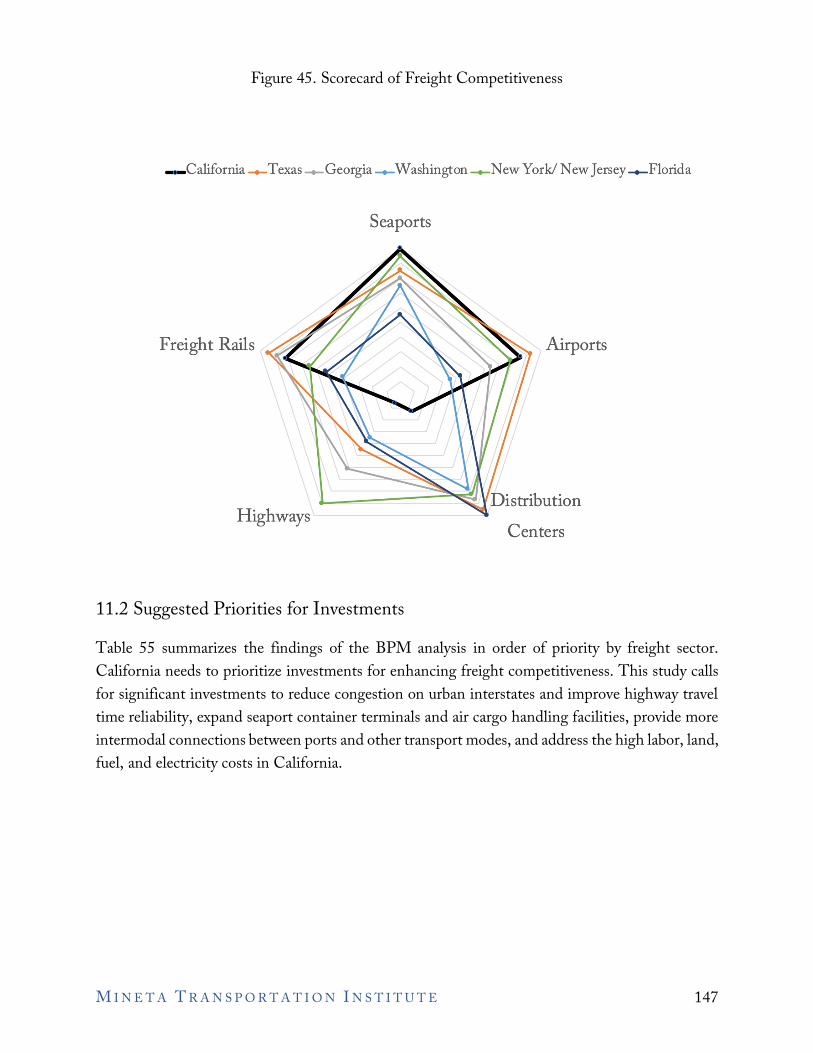
M I N E T A T R A N S P O R T A T I O N I N S T I T U T E 147
Figure 45. Scorecard of Freight Competitiveness
11.2 Suggested Priorities for Investments Table 55 summarizes the findings of the BPM analysis in order of priority by freight sector. California needs to prioritize investments for enhancing freight competitiveness. This study calls for significant investments to reduce congestion on urban interstates and improve highway travel time reliability, expand seaport container terminals and air cargo handling facilities, provide more intermodal connections between ports and other transport modes, and address the high labor, land, fuel, and electricity costs in California.
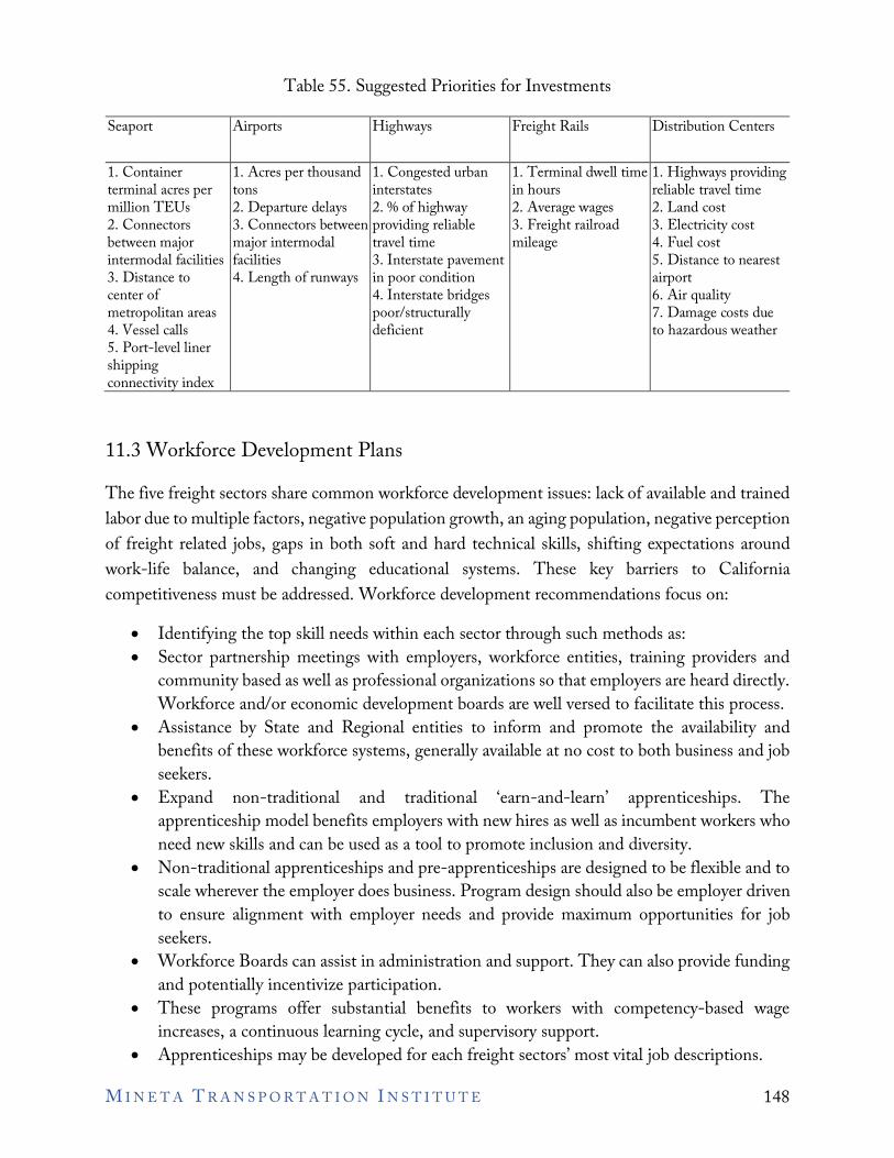
M I N E T A T R A N S P O R T A T I O N I N S T I T U T E 148
Table 55. Suggested Priorities for Investments
Seaport Airports Highways Freight Rails Distribution Centers
1. Container terminal acres per million TEUs 2. Connectors between major intermodal facilities 3. Distance to center of metropolitan areas 4. Vessel calls 5. Port-level liner shipping connectivity index
1. Acres per thousand tons 2. Departure delays 3. Connectors between major intermodal facilities 4. Length of runways
1. Congested urban interstates 2. % of highway providing reliable travel time 3. Interstate pavement in poor condition 4. Interstate bridges poor/structurally deficient
1. Terminal dwell time in hours 2. Average wages 3. Freight railroad mileage
1. Highways providing reliable travel time 2. Land cost 3. Electricity cost 4. Fuel cost 5. Distance to nearest airport 6. Air quality 7. Damage costs due to hazardous weather
11.3 Workforce Development Plans The five freight sectors share common workforce development issues: lack of available and trained labor due to multiple factors, negative population growth, an aging population, negative perception of freight related jobs, gaps in both soft and hard technical skills, shifting expectations around work-life balance, and changing educational systems. These key barriers to California competitiveness must be addressed. Workforce development recommendations focus on:
• Identifying the top skill needs within each sector through such methods as: • Sector partnership meetings with employers, workforce entities, training providers and
community based as well as professional organizations so that employers are heard directly. Workforce and/or economic development boards are well versed to facilitate this process.
• Assistance by State and Regional entities to inform and promote the availability and benefits of these workforce systems, generally available at no cost to both business and job seekers.
• Expand non-traditional and traditional ‘earn-and-learn’ apprenticeships. The apprenticeship model benefits employers with new hires as well as incumbent workers who need new skills and can be used as a tool to promote inclusion and diversity.
• Non-traditional apprenticeships and pre-apprenticeships are designed to be flexible and to scale wherever the employer does business. Program design should also be employer driven to ensure alignment with employer needs and provide maximum opportunities for job seekers.
• Workforce Boards can assist in administration and support. They can also provide funding and potentially incentivize participation.
• These programs offer substantial benefits to workers with competency-based wage increases, a continuous learning cycle, and supervisory support.
• Apprenticeships may be developed for each freight sectors’ most vital job descriptions.
• Ensure training includes: • An appreciation of and ability to adapt to automation of equipment, machine learning. • Basic computer skills to operate and maintain equipment, as well as to handle
documentation and read/process digitalized material from instructions to process controls, and timesheets and expense reports.
• Use of updated VR and AI training tools to enhance understanding and promote faster, more efficient, targeted learning.
• Employ California Workforce Development Board’s High Road Training Partnership (HRTP) model designed to form partnerships of industry leaders, employers, workers, and union representatives (as appropriate). The pilot project has proven:
• This definition of partnership promotes inclusion and immediate addressing of workforce and management needs.
• Builds collective expertise and a willingness to find win-win solutions. • Promotes continuous experimentation and refining of workforce development, thus
making each entity more responsive to change when all voices are at the table. • Improved alignment with educational and training providers to meet employer and
disadvantaged community needs. • A broader coalition expands opportunities to secure equity and positive outcomes for
underserved workers and communities by reaching out to local workforce and American Job Centers of California (AJCC).
A central workforce theme for all the industry sectors mentioned in this report is accessing the services of their local Workforce Development Board who can deliver no cost assistance to businesses and the public throughout California. Workforce Boards can provide job seekers with the skills and training they need to get the quality jobs they desire; they can also match a skilled workforce with employers needing to hire. Business can use these services at no cost. The Workforce Boards can help business with recruitment and training and in many cases provide wage subsidies to business to support successful employment of the participants that are looking for work. Workforce Boards can also assist the region with its long-term workforce development planning by acting as a convener and bringing stakeholders together to identify industry needs, and then coordinating efforts to meet those needs. The California Workforce boards have access to the funding needed to implement programs such as these, and the workforce development system is already set up and ready to assist communities and business to stay competitive in a global marketplace.
11.4 Limitations The lack of publicly available data creates important limitations for this study. While we have identified key drivers for seaports, airports, highway, rail service, and location decisions of distribution centers, performance measures are not available for some key drivers. We identified some performance measures, which industry experts validated. Moreover, through interviews with
M I N E T A T R A N S P O R T A T I O N I N S T I T U T E 149
industry experts, numerous additional ideal metrics were identified that could not be obtained across states. Another key limitation is the number of interviewees for each sector. With six experts included, it is possible that responses are biased in a way that misrepresents the industry’s competitiveness as a whole.
M I N E T A T R A N S P O R T A T I O N I N S T I T U T E 150
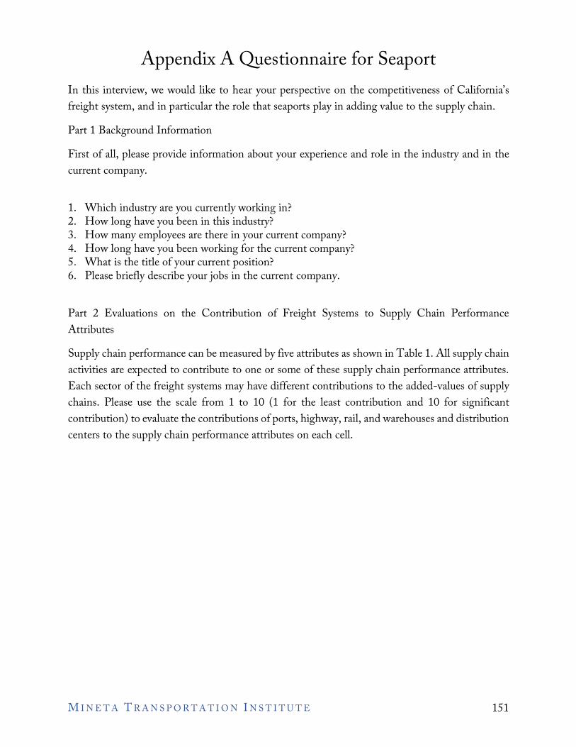
Appendix A Questionnaire for Seaport In this interview, we would like to hear your perspective on the competitiveness of California’s freight system, and in particular the role that seaports play in adding value to the supply chain. Part 1 Background Information First of all, please provide information about your experience and role in the industry and in the current company.
1. Which industry are you currently working in? 2. How long have you been in this industry? 3. How many employees are there in your current company? 4. How long have you been working for the current company? 5. What is the title of your current position? 6. Please briefly describe your jobs in the current company.
Part 2 Evaluations on the Contribution of Freight Systems to Supply Chain Performance Attributes Supply chain performance can be measured by five attributes as shown in Table 1. All supply chain activities are expected to contribute to one or some of these supply chain performance attributes. Each sector of the freight systems may have different contributions to the added-values of supply chains. Please use the scale from 1 to 10 (1 for the least contribution and 10 for significant contribution) to evaluate the contributions of ports, highway, rail, and warehouses and distribution centers to the supply chain performance attributes on each cell.
M I N E T A T R A N S P O R T A T I O N I N S T I T U T E 151
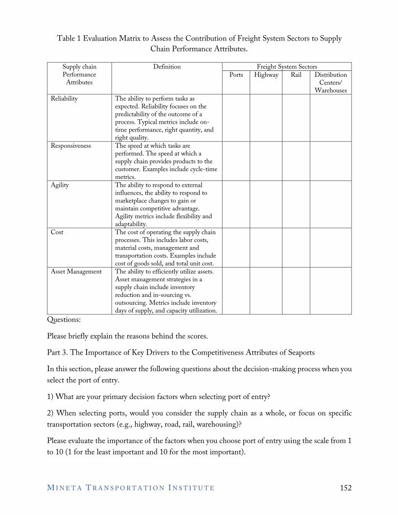
Table 1 Evaluation Matrix to Assess the Contribution of Freight System Sectors to Supply Chain Performance Attributes.
Supply chain Definition Freight System Sectors Performance
Attributes Ports Highway Rail Distribution
Centers/ Warehouses
Reliability The ability to perform tasks as expected. Reliability focuses on the predictability of the outcome of a process. Typical metrics include on-time performance, right quantity, and right quality.
Responsiveness The speed at which tasks are performed. The speed at which a supply chain provides products to the customer. Examples include cycle-time metrics.
Agility The ability to respond to external influences, the ability to respond to marketplace changes to gain or maintain competitive advantage. Agility metrics include flexibility and adaptability.
Cost The cost of operating the supply chain processes. This includes labor costs, material costs, management and transportation costs. Examples include cost of goods sold, and total unit cost.
Asset Management The ability to efficiently utilize assets. Asset management strategies in a supply chain include inventory reduction and in-sourcing vs. outsourcing. Metrics include inventory days of supply, and capacity utilization.
Questions: Please briefly explain the reasons behind the scores. Part 3. The Importance of Key Drivers to the Competitiveness Attributes of Seaports In this section, please answer the following questions about the decision-making process when you select the port of entry. 1) What are your primary decision factors when selecting port of entry? 2) When selecting ports, would you consider the supply chain as a whole, or focus on specific transportation sectors (e.g., highway, road, rail, warehousing)? Please evaluate the importance of the factors when you choose port of entry using the scale from 1 to 10 (1 for the least important and 10 for the most important).
M I N E T A T R A N S P O R T A T I O N I N S T I T U T E 152
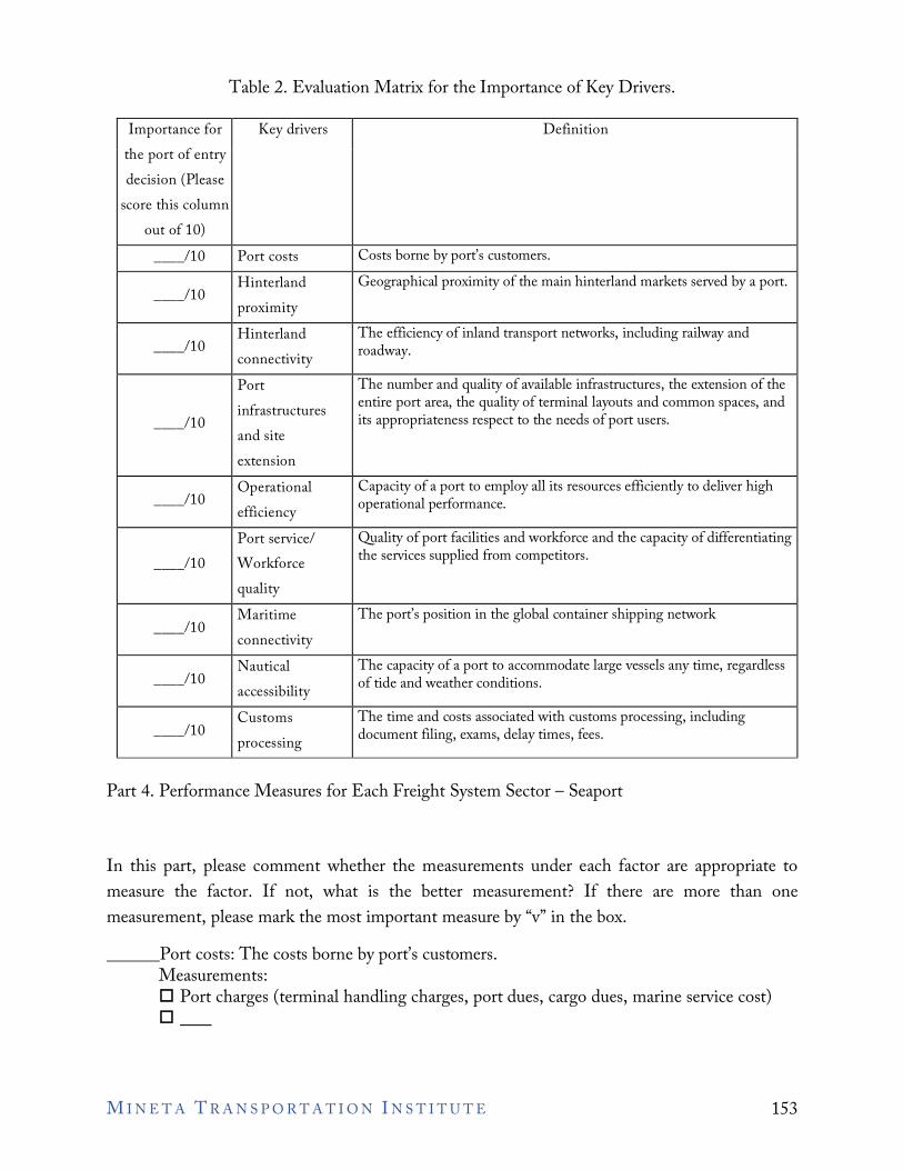
1
Table 2. Evaluation Matrix for the Importance of Key Drivers.
Importance for the port of entry decision (Please
score this column out of 10)
Key drivers Definition
____/10 Port costs Costs borne by port’s customers.
____/10 Hinterland proximity
Geographical proximity of the main hinterland markets served by a port.
____/10 Hinterland connectivity
The efficiency of inland transport networks, including railway and roadway.
____/10
Port infrastructures and site extension
The number and quality of available infrastructures, the extension of the entire port area, the quality of terminal layouts and common spaces, and its appropriateness respect to the needs of port users.
____/10 Operational efficiency
Capacity of a port to employ all its resources efficiently to deliver high operational performance.
____/10 Port service/ Workforce quality
Quality of port facilities and workforce and the capacity of differentiating the services supplied from competitors.
____/10 Maritime connectivity
The port’s position in the global container shipping network
____/10 Nautical accessibility
The capacity of a port to accommodate large vessels any time, regardless of tide and weather conditions.
____/10 Customs processing
The time and costs associated with customs processing, including document filing, exams, delay times, fees.
Part 4. Performance Measures for Each Freight System Sector – Seaport
In this part, please comment whether the measurements under each factor are appropriate to measure the factor. If not, what is the better measurement? If there are more than one measurement, please mark the most important measure by “v” in the box. ______Port costs: The costs borne by port’s customers.
Measurements: • Port charges (terminal handling charges, port dues, cargo dues, marine service cost) •
M I N E T A T R A N S P O R T A T I O N I N S T I T U T E 153
1
1
1
1
1
______Hinterland proximity: Hinterland proximity refers to the geographical proximity of the main hinterland markets served by a port. Measurements: • GDP of metropolitan area • Distance to center of metropolitan area •
______Hinterland connectivity: Hinterland connectivity refers to the efficiency of inland transport networks.
Measurements: • Availability of hinterland connections (enough feeder connections, sufficiently reliable
and congestion-free road, rail and inland waterway capacity) •
______Port infrastructures and site extension: Number and quality of available infrastructures, the extension of the entire port area, the quality of terminal layouts and common spaces, as well as its appropriateness respect to the needs of port users. Measurements: • Main Channel Water Depth • Cargo Throughput – TEUs • Vessel Calls • Tonnage • TEU • Container cranes versus annual TEUs • Availability of Drydock and Marine Railway •
______Operational efficiency: Capacity of a port to employ all its resources efficiently to deliver high operational performance.
Measurements: • Capacity in TEUs • Maximum Average Calls • Average Container Vessel Dwell Time Hours • Port Turnaround Time • Voyage productivity: how quickly a port loads/offloads containers • Truck visit time: time spent by trucks inside the terminal to deliver/pick up a container •
______Port service/Workforce quality: Port service quality refers to the quality of port facilities and the capacity of differentiating the services supplied from competitors. Measurements: • Absence of disruptions, such as labor disputes •
______Maritime connectivity: Maritime connectivity refers to the efficiency of shipping transport networks.
Measurements:
M I N E T A T R A N S P O R T A T I O N I N S T I T U T E 154
1
1
1
• Port-level liner shipping connectivity index (capturing the level of integration into the existing liner shipping network)
• Time needed to import from China. •
______Nautical accessibility: Nautical accessibility refers to the capacity of a port to accommodate large vessels at anytime, regardless of tide and weather conditions. It is affected by natural factors (e.g, depth of inland rivers, tide range, etc.) and the endowment of physical infrastructures (e.g., locks, breakwaters, etc.) Measurements: • Max Size of Vessel •
______Customs processing: The time and costs associated with customs processing undertaken by U.S. Customs and Border Protection (CBP) and partner government agencies. This includes: 1) Fees; 2) preparation and filing of, or work related to, documents (e.g., CF-28 “Request for Information”, CF-29 “Notice of Action”, CF-19 “Protest”, CF-3461, CF-4647, CF-7501), 3) Trade Exams (which occur when CBP personnel conduct inspections of specific cargo entries to ensure that the required duties and fees are collected and to prevent goods that are not legally entitled to enter U.S. commerce from entering. Decisions on trade exams for several product groups involve partner government agencies as well as CBP). Measurements: • CBP-related Fees • CBP document preparation and filing costs • Trade Exam delay times •
Part 5. The Freight System Performance of California and Other Regions In this questionnaire, you will evaluation the performance of California and other regions. Based on your experience with the airports in different regions, please check on the regions and airports that you are familiar with. Please evaluate the performance of California and other regions using the scale from 1 to 10 (1 for the worst and 10 for the best). You can refer to the performance data of the airports in each region provided by the investigators.
M I N E T A T R A N S P O R T A T I O N I N S T I T U T E 155
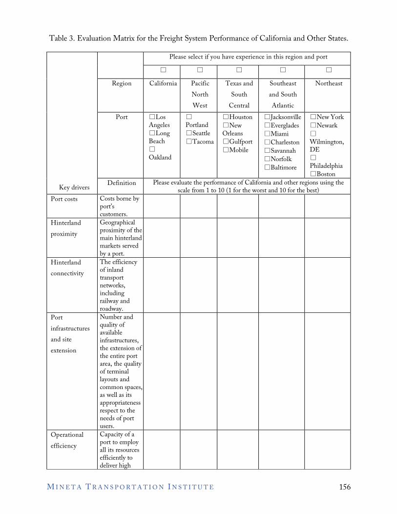
Table 3. Evaluation Matrix for the Freight System Performance of California and Other States.
Key drivers
Please select if you have experience in this region and port □ □ □ □ □
Region California Pacific North West
Texas and South
Central
Southeast and South Atlantic
Northeast
Port □Los Angeles □Long Beach □ Oakland
□ Portland □Seattle □Tacoma
□Houston □New Orleans □Gulfport □Mobile
□Jacksonville □Everglades □Miami □Charleston □Savannah □Norfolk □Baltimore
□New York □Newark □ Wilmington, DE □ Philadelphia □Boston
Definition Please evaluate the performance of California and other regions using the scale from 1 to 10 (1 for the worst and 10 for the best)
Port costs Costs borne by port’s customers.
Hinterland Geographical proximity proximity of the
main hinterland markets served by a port.
Hinterland The efficiency connectivity of inland
transport networks, including railway and roadway.
Port Number and infrastructures quality of
available and site infrastructures, extension the extension of
the entire port area, the quality of terminal layouts and common spaces, as well as its appropriateness respect to the needs of port users.
Operational Capacity of a efficiency port to employ
all its resources efficiently to deliver high
M I N E T A T R A N S P O R T A T I O N I N S T I T U T E 156
operational performance.
Port service/ Quality of port Workforce facilities and
workforce, and quality the capacity of
differentiating the services supplied from competitors.
Maritime The efficiency connectivity of shipping
transport networks in the world.
Nautical The capacity of accessibility a port to
accommodate large vessels any time, regardless of tide and weather conditions.
Customs The time and processing costs associated
with customs processing, including document filing, exams, delay times, fees.
Overall
Open-ended Questions
Please answer the following questions. A) Current state of California freight competitiveness: 1) Which ports/states are the key competitors to California in terms of ocean shipping? 2) What investments have been made recently to the infrastructure of ports? 3) Where are the key bottlenecks in the California’s port system? 4) Where are the key connections between port and other modes within California? Rail?
Roads? Do these connections impact competitiveness?
B) The future of California freight competitiveness: 1) How can the California’s ports become more competitive? 2) What investments need to be made to improve California’s port competitiveness? 3) What future trends are the major threats to California’s port competitiveness?
Part 6. California’s Freight System Performance with respect to Environmental, Sustainability, and Resilience Factors
M I N E T A T R A N S P O R T A T I O N I N S T I T U T E 157
Questions: 1) How resilient is California’s ports to disasters, to outages or accidents, or to economic
downturns? 2) What are some environmental impacts brought on by ocean shipping? What are the route
causes of the impacts? 3) What investments have been made recently to mitigate the environmental impact caused by
ports? 4) What investments need to be made to mitigate the environmental impact caused by ports? 5) How does the sustainability of ports affect the competitiveness of California? 6) Which current environmental regulations lead to extra burdens on firms?
M I N E T A T R A N S P O R T A T I O N I N S T I T U T E 158
Appendix B Questionnaire for Airport In this interview, we would like to hear your perspective on the competitiveness of California’s freight system, and in particular the role that airports play in adding value to the supply chain. Part 1 Background Information First of all, please provide information about your experience and role in the industry and in the current company.
1) Which industry are you currently working in? 2) How long have you been in this industry? 3) How many employees are there in your current company? 4) How long have you been working for the current company? 5) What is the title of your current position? 6) Please briefly describe your jobs in the current company.
Part 2 Evaluations on the Contribution of Freight Systems to Supply Chain Performance Attributes Supply chain performance can be measured by five attributes as shown in Table 1. All supply chain activities are expected to contribute to one or some of these supply chain performance attributes. Each sector of the freight systems may have different contributions to the added-values of supply chains. Please use the scale from 1 to 10 (1 for the least contribution and 10 for significant contribution) to evaluate the contributions of ports, highway, rail, and warehouses and distribution centers to the supply chain performance attributes on each cell.
M I N E T A T R A N S P O R T A T I O N I N S T I T U T E 159
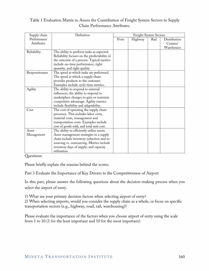
Table 1 Evaluation Matrix to Assess the Contribution of Freight System Sectors to Supply Chain Performance Attributes.
Supply chain Definition Freight System Sectors Performance Attributes
Ports Highway Rail Distribution Centers/
Warehouses Reliability The ability to perform tasks as expected.
Reliability focuses on the predictability of the outcome of a process. Typical metrics include on-time performance, right quantity, and right quality.
Responsiveness The speed at which tasks are performed. The speed at which a supply chain provides products to the customer. Examples include cycle-time metrics.
Agility The ability to respond to external influences, the ability to respond to marketplace changes to gain or maintain competitive advantage. Agility metrics include flexibility and adaptability.
Cost The cost of operating the supply chain processes. This includes labor costs, material costs, management and transportation costs. Examples include cost of goods sold, and total unit cost.
Asset Management
The ability to efficiently utilize assets. Asset management strategies in a supply chain include inventory reduction and in-sourcing vs. outsourcing. Metrics include inventory days of supply, and capacity utilization.
Questions: Please briefly explain the reasons behind the scores. Part 3 Evaluate the Importance of Key Drivers to the Competitiveness of Airport In this part, please answer the following questions about the decision-making process when you select the airport of entry. 1) What are your primary decision factors when selecting airport of entry? 2) When selecting airports, would you consider the supply chain as a whole, or focus on specific transportation sectors (e.g., highway, road, rail, warehousing)?
Please evaluate the importance of the factors when you choose airport of entry using the scale from 1 to 10 (1 for the least important and 10 for the most important).
M I N E T A T R A N S P O R T A T I O N I N S T I T U T E 160
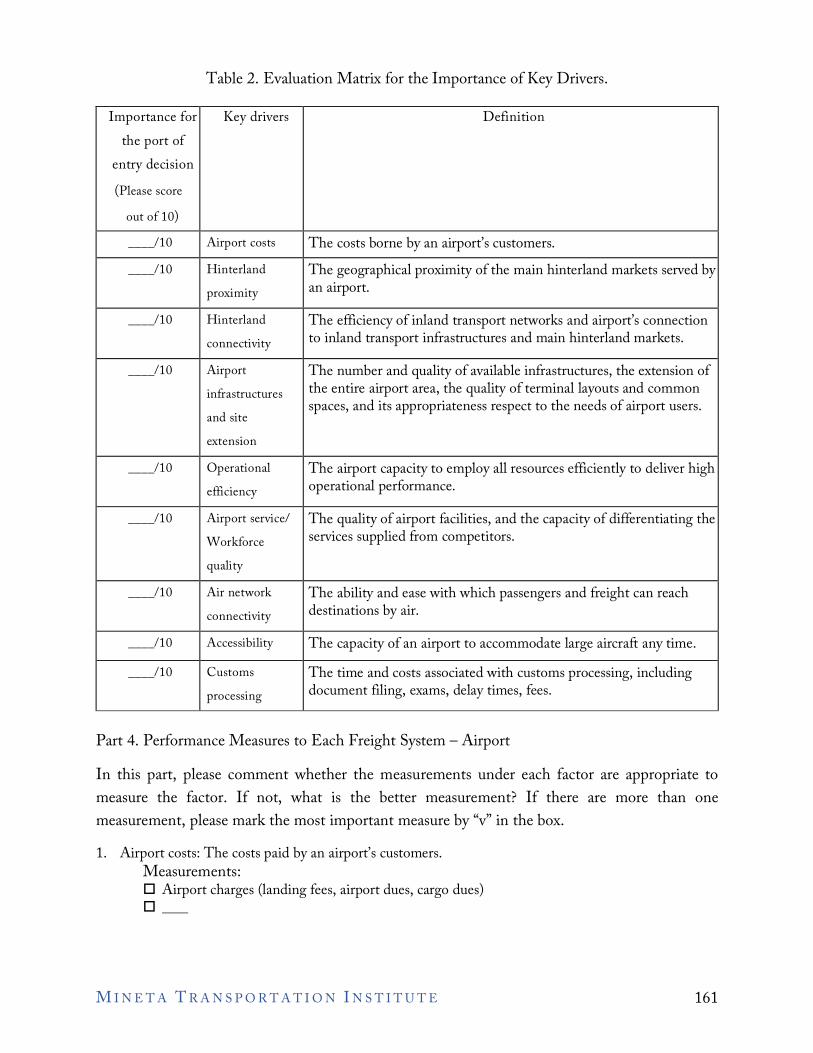
1
Table 2. Evaluation Matrix for the Importance of Key Drivers.
Importance for the port of
entry decision (Please score
out of 10)
Key drivers Definition
____/10 Airport costs The costs borne by an airport’s customers. ____/10 Hinterland
proximity The geographical proximity of the main hinterland markets served by an airport.
____/10 Hinterland connectivity
The efficiency of inland transport networks and airport’s connection to inland transport infrastructures and main hinterland markets.
____/10 Airport infrastructures and site extension
The number and quality of available infrastructures, the extension of the entire airport area, the quality of terminal layouts and common spaces, and its appropriateness respect to the needs of airport users.
____/10 Operational efficiency
The airport capacity to employ all resources efficiently to deliver high operational performance.
____/10 Airport service/ Workforce quality
The quality of airport facilities, and the capacity of differentiating the services supplied from competitors.
____/10 Air network connectivity
The ability and ease with which passengers and freight can reach destinations by air.
____/10 Accessibility The capacity of an airport to accommodate large aircraft any time. ____/10 Customs
processing The time and costs associated with customs processing, including document filing, exams, delay times, fees.
Part 4. Performance Measures to Each Freight System – Airport In this part, please comment whether the measurements under each factor are appropriate to measure the factor. If not, what is the better measurement? If there are more than one measurement, please mark the most important measure by “v” in the box. 1. Airport costs: The costs paid by an airport’s customers.
Measurements: • Airport charges (landing fees, airport dues, cargo dues) •
M I N E T A T R A N S P O R T A T I O N I N S T I T U T E 161
1
1
1
1
1
1
2. Hinterland proximity: The geographical proximity of the main hinterland markets served by an airport.
Measurements: • GDP of metropolitan area • Distance to center of metropolitan area •
3. Hinterland connectivity: The efficiency of inland transport networks and airport’s connection to inland transport infrastructures and main hinterland markets.
Measurements: • Availability of hinterland connections (enough feeder connections, sufficiently reliable and
congestion-free road) •
4. Airport infrastructures and site extension: The number and quality of available infrastructures, the extension of the entire airport area, the quality of terminal layouts and common spaces, and its appropriateness respect to the needs of airport users.
Measurements: • Number of carriers currently serving airport • Number of destinations • Existence of curfews • Acres of cargo-handling facilities •
5. Operational efficiency: Capacity of an airport to employ all its resources efficiently to deliver high operational performance.
Measurements: • Flight frequency by airlines with cargo capacity • Cargo growth • Tonnage of cargo • Export value/tonnage • Ranking of export value/tonnage among all U.S. airports • Import alue/tonnage • Ranking of import value/tonnage among all U.S. airports •
6. Airport service/Workforce quality: The quality of airport facilities, and the capacity of differentiating the services supplied from competitors.
Measurements: • Average departure delays • Average arrival delays • Percentage of cancelled flights • Airport service quality awards •
7. Air network connectivity: The ability and ease with which passengers and freight can reach destinations by air.
Measurements: • The OAG Megahubs International Index (measures the number of connections possible
within a specific time frame and the relative attractiveness of each airport as a connecting point for scheduled domestic air passengers)
•
M I N E T A T R A N S P O R T A T I O N I N S T I T U T E 162
1
1
8. Accessibility: Accessibility refers to the capacity of an airport to accommodate large aircraft any time. It is affected by natural factors and the endowment of physical infrastructures.
Measurements: • Max Size of Aircraft • Length of runway •
9. Customs processing: The time and costs associated with customs processing undertaken by U.S. Customs and Border Protection (CBP) and partner government agencies. This includes: 1) Fees; 2) preparation and filing of, or work related to, documents (e.g., CF-28 “Request for Information”, CF-29 “Notice of Action”, CF-19 “Protest”, CF-3461, CF-4647, CF-7501), 3) Trade Exams (which occur when CBP personnel conduct inspections of specific cargo entries to ensure that the required duties and fees are collected and to prevent goods that are not legally entitled to enter U.S. commerce from entering. Decisions on trade exams for several product groups involve partner government agencies as well as CBP).
Measurements: • CBP-related Fees • CBP document preparation and filing costs • Trade Exam delay times •
Part 5 Evaluate the Performance of California and other states In this questionnaire, you will evaluation the performance of California and other regions. Based on your experience with the airports in different regions, please check on the regions and airports that you are familiar with. Please evaluate the performance of California and other regions using the scale from 1 to 10 (1 for the worst and 10 for the best). You can refer to the performance data of the airports in each region provided by the investigators.
M I N E T A T R A N S P O R T A T I O N I N S T I T U T E 163
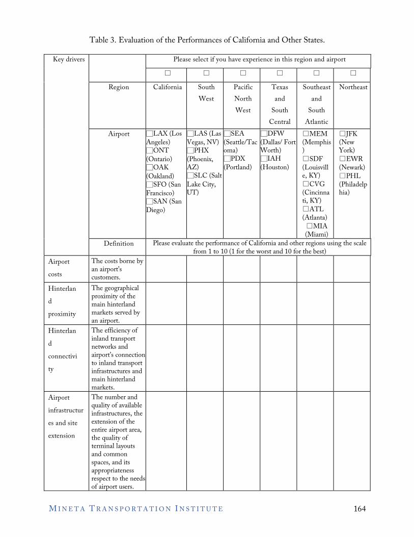
Table 3. Evaluation of the Performances of California and Other States.
Key drivers Please select if you have experience in this region and airport □ □ □ □ □ □
Region California South West
Pacific North West
Texas and
South Central
Southeast and
South Atlantic
Northeast
Airport □LAX (Los Angeles) □ONT (Ontario) □OAK (Oakland) □SFO (San Francisco) □SAN (San Diego)
□LAS (Las Vegas, NV) □PHX (Phoenix, AZ) □SLC (Salt Lake City, UT)
□SEA (Seattle/Tac oma) □PDX (Portland)
□DFW (Dallas/ Fort Worth) □IAH (Houston)
□MEM (Memphis ) □SDF (Louisvill e, KY) □CVG (Cincinna ti, KY) □ATL (Atlanta) □MIA (Miami)
□JFK (New York) □EWR (Newark) □PHL (Philadelp hia)
Definition Please evaluate the performance of California and other regions using the scale from 1 to 10 (1 for the worst and 10 for the best)
Airport costs
The costs borne by an airport’s customers.
Hinterlan The geographical d proximity of the
main hinterland proximity markets served by
an airport. Hinterlan The efficiency of d inland transport
networks and connectivi airport’s connection
to inland transport ty infrastructures and main hinterland markets.
Airport The number and infrastructur quality of available
infrastructures, the es and site extension of the
entire airport area, extension the quality of terminal layouts and common spaces, and its appropriateness respect to the needs of airport users.
M I N E T A T R A N S P O R T A T I O N I N S T I T U T E 164
Operation The capacity of an al airport to employ
all its resources efficiency efficiently to deliver
high operational performance.
Airport The quality of service/ airport facilities and
the capacity of Workforce differentiating the
services supplied quality from competitors. Air The ability and ease network with which
passengers and connectivi freight can reach
destinations by air. ty Accessibili The capacity of an
airport to ty accommodate large aircraft any time.
Customs The time and costs processing associated with
customs processing undertaken by U.S. Customs and Border Protection and partner government agencies.
Overall
Open-ended Questions Please answer the following questions. A) Current state of California freight competitiveness: 1) Which airports/states are the key competitors to California in terms of air shipping? 2) What investments have been made recently to the infrastructure of airports? 3) Where are the key bottlenecks in the California’s airport system? 4) Where are the key connections between airport and other modes within California? Rail? Roads? Do
these connections impact competitiveness?
B) The future of California freight competitiveness: 1) How can the California’s airports become more competitive? 2) What investments need to be made to improve California’s airport competitiveness? 3) What future trends are the major threats to California’s airport competitiveness?
Part 6 Evaluate the Performance of Environment
M I N E T A T R A N S P O R T A T I O N I N S T I T U T E 165
Questions: 1) How resilient is California’s LAX airport to disasters, to outages or accidents, or to economic
downturns? 2) What are some environmental impacts brought on by air shipping? What are the route causes of the
impacts? 3) What investments have been made recently to mitigate the environmental impact caused by airports? 4) What investments need to be made to mitigate the environmental impact caused by airports? 5) How does the sustainability of airports affect the competitiveness of California? 6) Which current environmental regulations lead to extra burdens on firms?
M I N E T A T R A N S P O R T A T I O N I N S T I T U T E 166
Appendix C Questionnaire for Highway In this interview, we would like to hear your perspective on the competitiveness of California’s freight system, and in particular the role that rail systems play in adding value to the supply chain. Part 1. Background Information First of all, please provide information about your experience and role in the industry and in your current company. 1) Which industry are you currently working in? 2) How long have you been in this industry? 3) How many employees are there in your current company? 4) How long have you been working for the current company? 5) What is the title of your current position? 6) Please briefly describe your jobs in the current company.
Part 2 Evaluations on the Contribution of Freight Systems to Supply Chain Performance Attributes Each sector of the freight systems may have different contributions to the added-values of supply chains. Please use the scale from 1 to 10 (1 for the least contribution and 10 for significant contribution) to evaluate the contributions of ports, highway, rail, and warehouses and distribution centers to the supply chain performance attributes on each cell.
M I N E T A T R A N S P O R T A T I O N I N S T I T U T E 167
Table 1. Evaluation Matrix to Assess the Contribution of Freight System Sectors to Supply Chain Performance Attributes.
Supply chain Performance
Attributes
Freight System Sectors
Ports Highway Rail Distribution
Centers/ Warehouses
Reliability
The ability to perform tasks as expected. Reliability focuses on the predictability of the outcome of a process. Typical metrics for the reliability attributes include on-time performance, right quantity, and right quality.
Responsiveness
The speed at which tasks are performed. The speed at which a supply chain provides products to the customer. Examples include cycle-time metrics.
Agility
The ability to respond to external influences, the ability to respond to marketplace changes to gain or maintain competitive advantage. Agility metrics include flexibility and adaptability.
Cost
The cost of operating the supply chain processes. This includes labor costs, material costs, management and transportation costs. Examples include cost of goods sold, and total unit cost.
Asset Management
The ability to efficiently utilize assets. Asset management strategies in a supply chain include inventory reduction and in-sourcing vs. outsourcing. Metrics include inventory days of supply, and capacity utilization.
Questions: Please briefly explain the reasons behind the scores. Part 3 Evaluate the Importance and Contribution of Key Drivers to the Competitiveness of the Highway system Please evaluate the importance of the factors when you choose a highway system using the scale from 1 to 10 (1 for the least important and 10 for the most important). In addition, please mark “V” if the key driver is associated with the supply chain performance attributes. Table 2 Evaluation of the Importance and Contribution of Key Drivers to the Competitiveness of the Highway System
M I N E T A T R A N S P O R T A T I O N I N S T I T U T E 168
1
Importan Key drivers Definition Reliabili Responsi Agility Cost Asset ce for ty ve-ness Mgmt
choosing (resilien (turns, a (on- (speed) ce, (total cash
highway time, flexibilit cost) cycle) system order
fill) y)
Safety The physical safety of drivers moving goods across the highway system and the general public.
Maintena The physical conditions of nce and highways and bridges.
Preservati on Mobility The ability to move and through the highway Congestio system and the time it n takes to move goods
across the highway system.
Mobility and Reliability
The ability to move through the highway system at consistent speeds and without major delays.
Accessibil ity
The ability of good-movers to access the highway system in an efficient manner.
Connectiv ity
Capacity of highway system to allow fast movement of goods across connected highway sectors.
Part 4. Performance Measures to Each Freight System – Highway In this part, please comment whether the measurements under each factor are appropriate to measure the factor. If not, what is the better measurement?
1. Safety: The physical safety of drivers moving goods across the highway system and the general public. Measurements: • Number of all traffic collisions and percentage involving freight trucks. • Number of all traffic fatalities and percentage involving freight trucks. • Truck parking availability • Rest area availability •
M I N E T A T R A N S P O R T A T I O N I N S T I T U T E 169
1
1
1
1
1
2. Maintenance and Preservation: The physical conditions of highways and bridges. Measurements: • Percentage of highway pavement in good condition. • Percentage of highway bridges and connectors in good condition. •
3. Mobility and Congestion: The ability to move through the highway system and the time it takes to move goods across the highway system. Measurements: • Truck Travel Time (TTT) • Truck Volume • Truck-to-Car Travel Ratio (TTR) • Percentage of highway uncongested • Border crossing inbound truck volume •
4. Mobility and Reliability: The ability to move through the highway system at consistent speeds and without major delays. Measurements: • Percentage of highway providing reliable travel time • Accident clearing time • Border crossing average wait time •
5. Accessibility: The ability of good-movers to access the highway system in an efficient manner. Measurements: • Percentage of major generators with appropriate roadway access to corridors and major
highways •
6. Connectivity: Capacity of highway system to allow fast movement of goods across connected highway sectors. Measurements: • Percentage of shippers with access to triple network, triple trailer • Number of connections • Border crossing number of lanes •
Part 5 Evaluate the Performance of California and other regions – Highway System Based on your experience with the highway system in different regions, please write down the name of regions and highways. Please evaluate the performance of California and other regions using the scale from 1 to 10 (1 for the worst and 10 for the best). You can refer to the performance data of each port provided by the investigators.
M I N E T A T R A N S P O R T A T I O N I N S T I T U T E 170
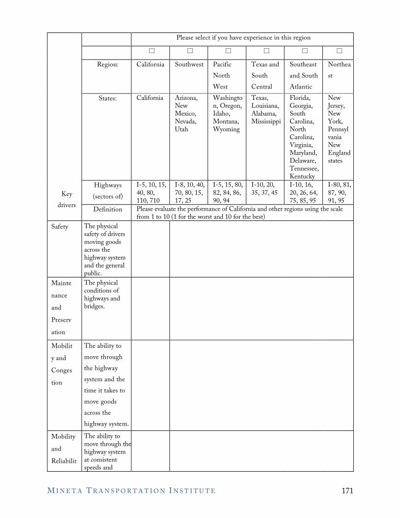
Key drivers
Please select if you have experience in this region □ □ □ □ □ □
Region: California Southwest Pacific North West
Texas and South Central
Southeast and South Atlantic
Northea st
States: California Arizona, New Mexico, Nevada, Utah
Washingto n, Oregon, Idaho, Montana, Wyoming
Texas, Louisiana, Alabama, Mississippi
Florida, Georgia, South Carolina, North Carolina, Virginia, Maryland, Delaware, Tennessee, Kentucky
New Jersey, New York, Pennsyl vania New England states
Highways (sectors of)
I-5, 10, 15, 40, 80, 110, 710
I-8, 10, 40, 70, 80, 15, 17, 25
I-5, 15, 80, 82, 84, 86, 90, 94
I-10, 20, 35, 37, 45
I-10, 16, 20, 26, 64, 75, 85, 95
I-80, 81, 87, 90, 91, 95
Definition Please evaluate the performance of California and other regions using the scale from 1 to 10 (1 for the worst and 10 for the best)
Safety The physical safety of drivers moving goods across the highway system and the general public.
Mainte The physical conditions of nance highways and
and bridges. Preserv ation Mobilit The ability to y and move through Conges the highway tion system and the
time it takes to move goods across the highway system.
Mobility The ability to and move through the
highway system Reliabilit at consistent
speeds and
M I N E T A T R A N S P O R T A T I O N I N S T I T U T E 171
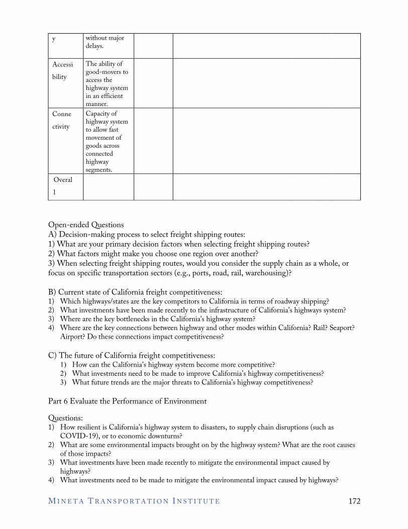
y without major delays.
Accessi The ability of bility good-movers to
access the highway system in an efficient manner.
Conne Capacity of ctivity highway system
to allow fast movement of goods across connected highway segments.
Overal l
Open-ended Questions A) Decision-making process to select freight shipping routes: 1) What are your primary decision factors when selecting freight shipping routes? 2) What factors might make you choose one region over another? 3) When selecting freight shipping routes, would you consider the supply chain as a whole, or focus on specific transportation sectors (e.g., ports, road, rail, warehousing)?
B) Current state of California freight competitiveness: 1) Which highways/states are the key competitors to California in terms of roadway shipping? 2) What investments have been made recently to the infrastructure of California’s highways system? 3) Where are the key bottlenecks in the California’s highway system? 4) Where are the key connections between highway and other modes within California? Rail? Seaport?
Airport? Do these connections impact competitiveness?
C) The future of California freight competitiveness: 1) How can the California’s highway system become more competitive? 2) What investments need to be made to improve California’s highway competitiveness? 3) What future trends are the major threats to California’s highway competitiveness?
Part 6 Evaluate the Performance of Environment Questions: 1) How resilient is California’s highway system to disasters, to supply chain disruptions (such as
COVID-19), or to economic downturns? 2) What are some environmental impacts brought on by the highway system? What are the root causes
of those impacts? 3) What investments have been made recently to mitigate the environmental impact caused by
highways? 4) What investments need to be made to mitigate the environmental impact caused by highways?
M I N E T A T R A N S P O R T A T I O N I N S T I T U T E 172
5) How does the sustainability of highways affect the competitiveness of California? 6) Which current environmental regulations lead to extra burdens on firms?
M I N E T A T R A N S P O R T A T I O N I N S T I T U T E 173
Appendix D Questionnaire for Freight Rail In this interview, we would like to hear your perspective on the competitiveness of California’s freight system, and in particular the role that rail systems play in adding value to the supply chain. First of all, please provide information about your experience and role in the industry and in the current company. 1) Which industry are you currently working in? 2) How long have you been in this industry? 3) How many employees are there in your current company? 4) How long have you been working for the current company? 5) What is the title of your current position at this company? 6) Please briefly describe your roles in your current position.
Part 1. Evaluate the Contribution of Freight System Sectors to Supply Chain Performance Attributes
Each sector of the freight systems may have different contributions to the added-values of supply chains. Please use the scale from 1 to 10 (1 for the least contribution and 10 for significant contribution) to evaluate the contributions of ports, highway, rail, and warehouses and distribution centers to the supply chain performance attributes on each cell.
M I N E T A T R A N S P O R T A T I O N I N S T I T U T E 174
Table 1. Evaluation Matrix to Assess the Contribution of Freight System Sectors to Supply Chain Performance Attributes.
Supply chain Performance
Definition Freight System Sectors
Attributes Ports Highway Rail Warehouse/ Distribution Center
Reliability The ability to perform tasks as expected. Reliability focuses on the predictability of the outcome of a process. Typical metrics for the reliability attributes include “On-time performance” and “Right quantity, right quality”.
Responsiveness The speed at which tasks are performed. The speed at which a supply chain provides products to the customer. Examples include “Cycle-time” metrics.
Agility The ability to respond to external influences, the ability to respond to marketplace changes to gain or maintain competitive advantage. Agility metrics include “Flexibility” and “Adaptability”.
Cost The cost of operating the supply chain processes. This includes labor costs, material costs, and management and transportation costs. Examples include “Cost of Goods Sold”, and “Unit Cost”.
Asset Management
The ability to efficiently utilize assets. Asset management strategies in a supply chain include inventory reduction and “In-sourcing vs. outsourcing”. Metrics include: “Inventory days of supply”, and “Capacity utilization”.
Questions: Please briefly explain the reasons behind the scores. Part 2. Evaluate the Importance and Contribution of Key Drivers to the Competitiveness of Rail Please evaluate the importance of the factors when you choose location of rail using the scale from 1 to 10 (1 for the least important and 10 for the most important). In addition, please mark “V” if the key driver is associated with the supply chain performance attributes.
M I N E T A T R A N S P O R T A T I O N I N S T I T U T E 175
Table 2. Evaluation Matrix to Assess the Importance and Contribution of Key Drivers to the Competitiveness of Rail.
Importance for the port
of entry decision
(Please score out of 10)
Key drivers
Definition Reliability
(on-time, order fill)
Responsi ve-ness
(speed)
Agility
(resilienc e,
flexibility )
Cost
(total cost)
Asset Mgmt
(turns, cash
cycle)
____/10 Cost Costs borne by rail customers
____/10 Hinterlan d proximity
Geographical proximity of the main hinterland markets served by rail system.
____/10 Hinterlan d connectivi ty
Hinterland connectivity refers to the efficiency of inland transport networks, including ports and roadway.
____/10 Operation al efficiency
Capacity of a rail system to employ all its resources efficiently to deliver high operational performance.
____/10 Rail service/ Workforce quality
Quality of (all) rail facilities and workforce, and to the capacity of differentiating the services supplied from competitors.
Questions: Do the key drivers above cover all important drivers that determine the competitiveness of the rail system? If not, which key driver(s) should be added? Part 3. Performance Measures to Each Freight System – Rail Please comment whether the indicators under each factor are appropriate to measure the factor. If not, what would be better indicators? If there are multiple indicators, please mark the most important measure by “v” in the box.
M I N E T A T R A N S P O R T A T I O N I N S T I T U T E 176
1
1
1
1
1
______Cost: The costs borne by rail customers. Indicators: • Rail charges •
______Hinterland proximity: Hinterland proximity refers to the geographical proximity of the main hinterland markets served by a rail system. Indicators: • GDP of metropolitan area • Distance to center of metropolitan area •
______Hinterland connectivity: Hinterland connectivity refers to the efficiency of inland transport networks.
Indicators: • Availability of hinterland connections (enough feeder connections, sufficiently reliable and
congestion-free road, port and inland waterway capacity) •
______Operational efficiency: Capacity of a rail system to employ all resources efficiently to deliver high operational performance.
Indicators: • Weekly carloads • Revenue ton miles • Freight car velocity • Train velocity • Switch and run-through car dwell • Operating car inventory • AAR Train speed • Terminal dwell •
______Rail service/Workforce quality: Rail service quality refers to the quality of (all) rail facilities, and to the capacity of differentiating the services supplied from competitors. Indicators: • Absence of labor dispute •
Part 4. Evaluate the Performance of California and other states - Rail
M I N E T A T R A N S P O R T A T I O N I N S T I T U T E 177
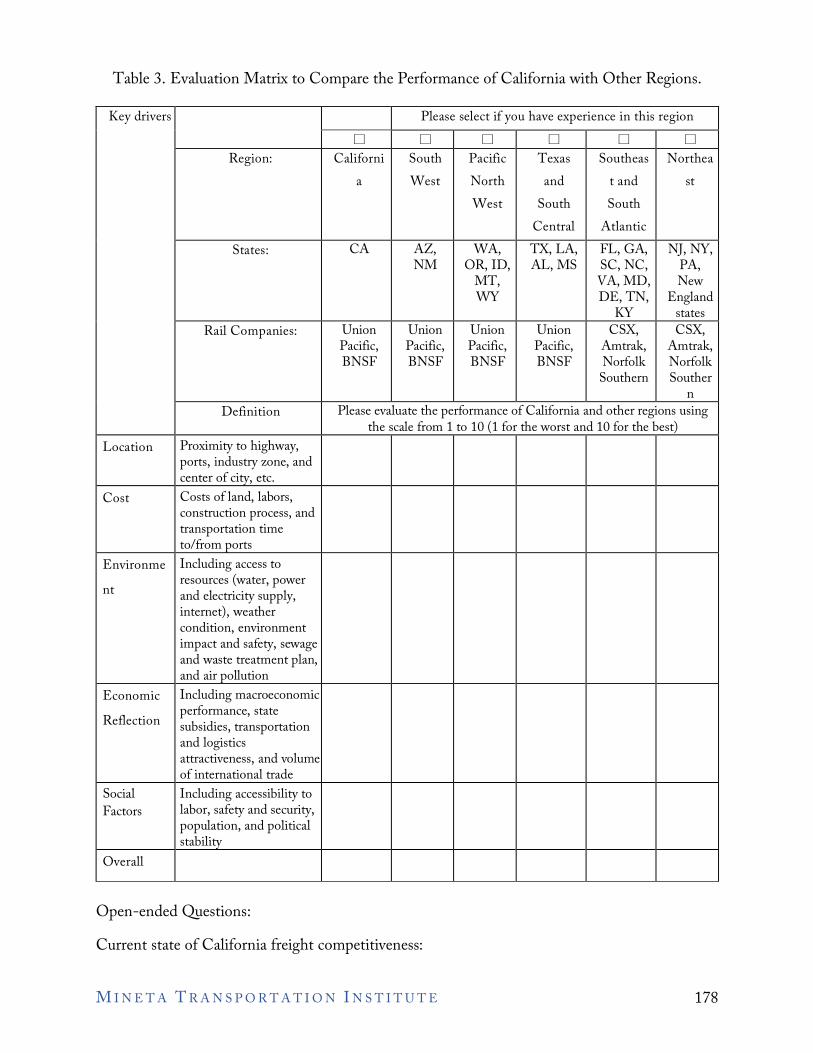
Table 3. Evaluation Matrix to Compare the Performance of California with Other Regions.
Key drivers Please select if you have experience in this region □ □ □ □ □ □
Region: Californi a
South West
Pacific North West
Texas and
South Central
Southeas t and South
Atlantic
Northea st
States: CA AZ, NM
WA, OR, ID,
MT, WY
TX, LA, AL, MS
FL, GA, SC, NC, VA, MD, DE, TN,
KY
NJ, NY, PA, New
England states
Rail Companies: Union Pacific, BNSF
Union Pacific, BNSF
Union Pacific, BNSF
Union Pacific, BNSF
CSX, Amtrak, Norfolk
Southern
CSX, Amtrak, Norfolk Souther
n Definition Please evaluate the performance of California and other regions using
the scale from 1 to 10 (1 for the worst and 10 for the best) Location Proximity to highway,
ports, industry zone, and center of city, etc.
Cost Costs of land, labors, construction process, and transportation time to/from ports
Environme nt
Including access to resources (water, power and electricity supply, internet), weather condition, environment impact and safety, sewage and waste treatment plan, and air pollution
Economic Reflection
Including macroeconomic performance, state subsidies, transportation and logistics attractiveness, and volume of international trade
Social Factors
Including accessibility to labor, safety and security, population, and political stability
Overall
Open-ended Questions: Current state of California freight competitiveness:
M I N E T A T R A N S P O R T A T I O N I N S T I T U T E 178
1) Which states are the key competitors to California in terms of rail system? 2) What recent investments California’s rail infrastructure have been game changers for the freight
industry? 3) Where are the key bottlenecks in the California’s rail system? 4) Where are the key connections between rail and transportation modes within California? Roads?
Ports? Airport? Do these connections impact competitiveness?
The future of California freight competitiveness: 1) What investments need to be made to improve California’s competitiveness in rail system? 2) How can California’s rail system become more competitive? 3) What future trends are the major threats to California’s rail system competitiveness?
Part 5. Evaluate the Performance with respect to the Environment, Sustainability, and Resilience
Questions: 1) How resilient is California’s rail system to disasters, to outages or accidents, or to economic
downturns? 2) What investments can to be made to mitigate the environmental impact caused by rail? 3) Which current environmental regulations lead to extra burdens on firms?
M I N E T A T R A N S P O R T A T I O N I N S T I T U T E 179
Appendix E Questionnaire for Distribution Center In this interview, we would like to hear your perspective on the competitiveness of California’s freight system, and in particular the role that distribution centers and warehouses play in adding value to the supply chain. Part 1 Background Informatio First of all, please provide information about your experience and role in the industry and in the current company.
1) Which industry are you currently working in? 2) How long have you been in this industry? 3) How many employees are there in your current company? 4) How long have you been working for the current company? 5) What is the title of your current position? 6) Please briefly describe your jobs in the current company.
Part 2 Evaluations on the Contribution of Freight Systems to Supply Chain Performance Attributes
Supply chain performance can be measured by five attributes as shown in Table 1. All supply chain activities are expected to contribute to one or some of these supply chain performance attributes. Each sector of the freight systems may have different contributions to the added-values of supply chains. Please use the scale from 1 to 10 (1 for the least contribution and 10 for significant contribution) to evaluate the contributions of ports, highway, rail, and warehouses and distribution centers to the supply chain performance attributes on each cell.
M I N E T A T R A N S P O R T A T I O N I N S T I T U T E 180
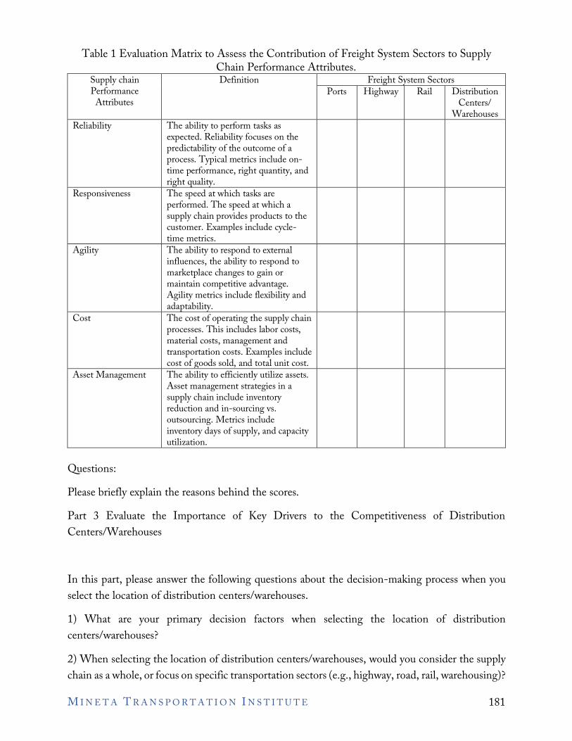
Table 1 Evaluation Matrix to Assess the Contribution of Freight System Sectors to Supply Chain Performance Attributes.
Supply chain Definition Freight System Sectors Performance Attributes
Ports Highway Rail Distribution Centers/
Warehouses Reliability The ability to perform tasks as
expected. Reliability focuses on the predictability of the outcome of a process. Typical metrics include on-time performance, right quantity, and right quality.
Responsiveness The speed at which tasks are performed. The speed at which a supply chain provides products to the customer. Examples include cycle-time metrics.
Agility The ability to respond to external influences, the ability to respond to marketplace changes to gain or maintain competitive advantage. Agility metrics include flexibility and adaptability.
Cost The cost of operating the supply chain processes. This includes labor costs, material costs, management and transportation costs. Examples include cost of goods sold, and total unit cost.
Asset Management The ability to efficiently utilize assets. Asset management strategies in a supply chain include inventory reduction and in-sourcing vs. outsourcing. Metrics include inventory days of supply, and capacity utilization.
Questions: Please briefly explain the reasons behind the scores. Part 3 Evaluate the Importance of Key Drivers to the Competitiveness of Distribution Centers/Warehouses
In this part, please answer the following questions about the decision-making process when you select the location of distribution centers/warehouses. 1) What are your primary decision factors when selecting the location of distribution centers/warehouses? 2) When selecting the location of distribution centers/warehouses, would you consider the supply chain as a whole, or focus on specific transportation sectors (e.g., highway, road, rail, warehousing)?
M I N E T A T R A N S P O R T A T I O N I N S T I T U T E 181
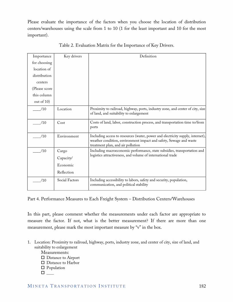
1
Please evaluate the importance of the factors when you choose the location of distribution centers/warehouses using the scale from 1 to 10 (1 for the least important and 10 for the most important).
Table 2. Evaluation Matrix for the Importance of Key Drivers.
Importance for choosing location of distribution
centers (Please score this column out of 10)
Key drivers Definition
____/10 Location Proximity to railroad, highway, ports, industry zone, and center of city, size of land, and suitability to enlargement
____/10 Cost Costs of land, labor, construction process, and transportation time to/from ports
____/10 Environment Including access to resources (water, power and electricity supply, internet), weather condition, environment impact and safety, Sewage and waste treatment plan, and air pollution
____/10 Cargo Capacity/ Economic Reflection
Including macroeconomic performance, state subsidies, transportation and logistics attractiveness, and volume of international trade
____/10 Social Factors Including accessibility to labors, safety and security, population, communication, and political stability
Part 4. Performance Measures to Each Freight System – Distribution Centers/Warehouses
In this part, please comment whether the measurements under each factor are appropriate to measure the factor. If not, what is the better measurement? If there are more than one measurement, please mark the most important measure by “v” in the box.
1. Location: Proximity to railroad, highway, ports, industry zone, and center of city, size of land, and suitability to enlargement
Measurements: • Distance to Airport • Distance to Harbor • Population •
M I N E T A T R A N S P O R T A T I O N I N S T I T U T E 182
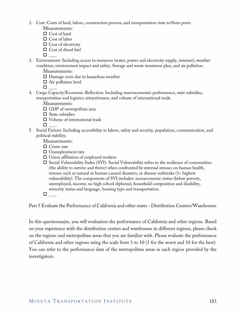
1
1
1
1
2. Cost: Costs of land, labors, construction process, and transportation time to/from ports. Measurements: • Cost of land • Cost of labor • Cost of electricity • Cost of diesel fuel •
3. Environment: Including access to resources (water, power and electricity supply, internet), weather condition, environment impact and safety, Sewage and waste treatment plan, and air pollution.
Measurements: • Damage costs due to hazardous weather • Air pollution level •
4. Cargo Capacity/Economic Reflection: Including macroeconomic performance, state subsidies, transportation and logistics attractiveness, and volume of international trade.
Measurements: • GDP of metropolitan area • State subsidies • Volume of international trade •
5. Social Factors: Including accessibility to labors, safety and security, population, communication, and political stability.
Measurements: • Crime rate • Unemployment rate • Union affiliation of employed workers • Social Vulnerability Index (SVI): Social Vulnerability refers to the resilience of communities
(the ability to survive and thrive) when confronted by external stresses on human health, stresses such as natural or human-caused disasters, or disease outbreaks (1= highest vulnerability). The components of SVI includes: socioeconomic status (below poverty, unemployed, income, no high school diploma), household composition and disability, minority status and language, housing type and transportation.
•
Part 5 Evaluate the Performance of California and other states - Distribution Centers/Warehouses
In this questionnaire, you will evaluation the performance of California and other regions. Based on your experience with the distribution centers and warehouses in different regions, please check on the regions and metropolitan areas that you are familiar with. Please evaluate the performance of California and other regions using the scale from 1 to 10 (1 for the worst and 10 for the best). You can refer to the performance data of the metropolitan areas in each region provided by the investigators.
M I N E T A T R A N S P O R T A T I O N I N S T I T U T E 183
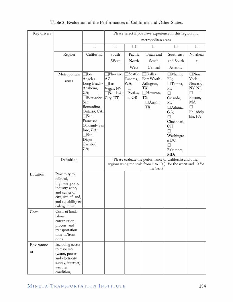
Table 3. Evaluation of the Performances of California and Other States.
Key drivers Please select if you have experience in this region and metropolitan areas
□ □ □ □ □ □
Region California South West
Pacific North West
Texas and South
Central
Southeast and South Atlantic
Northeas t
Metropolitan □Los □Phoenix, □Seattle- □Dallas- □Miami, □New areas Angeles-
Long Beach-Anaheim, CA; □Riverside-San Bernardino-Ontario, CA; □San Francisco-Oakland- San Jose, CA; □San Diego-Carlsbad, CA;
AZ □Las Vegas, NV □Salt Lake City, UT
Tacoma, WA; □ Portlan d, OR
Fort Worth-Arlington, TX; □Houston, TX; □Austin, TX;
FL; □Tampa, FL □ Orlando, FL □Atlanta, GA; □ Cincinnati, OH; □ Washingto n DC □ Baltimore, MD;
York-Newark, NY-NJ; □ Boston, MA □ Philadelp hia, PA
Definition Please evaluate the performance of California and other regions using the scale from 1 to 10 (1 for the worst and 10 for
the best) Location Proximity to
railroad, highway, ports, industry zone, and center of city, size of land, and suitability to enlargement
Cost Costs of land, labors, construction process, and transportation time to/from ports
Environme Including access to resources nt (water, power and electricity supply, internet), weather condition,
M I N E T A T R A N S P O R T A T I O N I N S T I T U T E 184
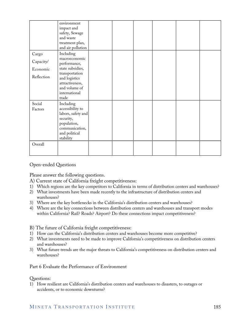
environment impact and safety, Sewage and waste treatment plan, and air pollution
Cargo Including Capacity/ macroeconomic
performance, Economic state subsidies,
transportation Reflection and logistics attractiveness, and volume of international trade
Social Including Factors accessibility to
labors, safety and security, population, communication, and political stability
Overall
Open-ended Questions Please answer the following questions. A) Current state of California freight competitiveness: 1) Which regions are the key competitors to California in terms of distribution centers and warehouses? 2) What investments have been made recently to the infrastructure of distribution centers and
warehouses? 3) Where are the key bottlenecks in the California’s distribution centers and warehouses? 4) Where are the key connections between distribution centers and warehouses and transport modes
within California? Rail? Roads? Airport? Do these connections impact competitiveness?
B) The future of California freight competitiveness: 1) How can the California’s distribution centers and warehouses become more competitive? 2) What investments need to be made to improve California’s competitiveness on distribution centers
and warehouses? 3) What future trends are the major threats to California’s competitiveness on distribution centers and
warehouses?
Part 6 Evaluate the Performance of Environment
Questions: 1) How resilient are California’s distribution centers and warehouses to disasters, to outages or
accidents, or to economic downturns?
M I N E T A T R A N S P O R T A T I O N I N S T I T U T E 185
2) What are some environmental impacts brought on by distribution centers and warehouses? What are the route causes of the impacts?
3) What investments have been made recently to mitigate the environmental impact caused by distribution centers and warehouses?
4) What investments need to be made to mitigate the environmental impact caused by distribution centers and warehouses?
5) How does the sustainability of distribution centers and warehouses affect the competitiveness of California?
6) Which current environmental regulations lead to extra burdens on firms?
M I N E T A T R A N S P O R T A T I O N I N S T I T U T E 186
Bibliography Aditjandra, Paulus T., Thomas H. Zunder, Dewan Md Zahurul Islam, and Roberto Palacin.
“Green rail transportation: improving rail freight to support green corridors.” In Green Transportation Logistics, 413-454. Springer, Cham, 2016.
Albert, Adrian, and Andreas Schaefer. “Demand for freight transportation in the US: a high-level view.” In 54th Annual Transportation Research Forum. Annapolis, Maryland, March 21-23, 2013 (No. 206946). Transportation Research Forum.
Ali, Fareeha. “How the coronavirus is changing ecommerce.” Digital Commerce 360. (February 15, 2021). https://www.digitalcommerce360.com/2021/02/15/ecommerce-during-coronavirus-pandemic-in-charts/#:~:text=Consumers%20spent%20%24861.12%20billion%20online,with%2015.8% 25%20the%20year%20prior.
Arvis, Jean-François, Lauri Ojala, Christina Wiederer, Ben Shepherd, Anasuya Raj, Karlygash Dairabayeva, and Tuomas Kiiski . Connecting to compete 2018: trade logistics in the global economy. (2018). World Bank, Washington, DC.
Barbour, William, Juan Carlos Martinez Mori, Shankara Kuppa, and Daniel B. Work. “Prediction of arrival times of freight traffic on US railroads using support vector regression.” Transportation Research Part C: Emerging Technologies, 93, (2018): 211-227.
Bitzan, John D., and Theodore E. Keeler. “The evolution of US rail freight pricing in the post-deregulation era: revenues versus marginal costs for five commodity types.” Transportation, 41, no.2 (2014): 305-324.
Bosquet, Romain, and Olivier Cazier. “Well-to-wheel energy comparison of US and European rail freight”. In 3rd International Conference on Road and Rail Infrastructure. (February, 2017).
Boyer, Kenneth D. “Why is the rail share of US freight traffic so low?” Journal of Transport Economics and Policy (JTEP), 48, no.2 (2014): 333-344.
Bureau of Transportation Statistics. (2017). “Freight facts and figures 2017.” https://www.bts.gov/newsroom/freight-facts-and-figures-2017.
Burnson, Patrick. “Top 30 U.S. ports: big ports got bigger in 2020.” Logistics Management (2021). https://www.logisticsmgmt.com/article/top_30_u.s._ports_big_ports_got_bigger_in_202 0.
M I N E T A T R A N S P O R T A T I O N I N S T I T U T E 187
� � � � �
� �
California Chamber of Commerce. (2018). “U.S. commerce report: California maintains position as top exporting state.” https://advocacy.calchamber.com/2018/03/13/us-commerce-report-california-maintains-position-as-top-exporting-state/.
California Chamber of Commerce. (2019). ‘Trade statistics.” https://advocacy.calchamber.com/international/trade/trade-statistics/.
Caltrans. (2021). “Freight railroad liaison – program overview.” https://dot.ca.gov/programs/rail-and-mass-transportation/freight-railroad-liaison.
Chadwick, Samantha G., Nanyan Zhou, and Mohd Rapik Saat. “Highway-rail grade crossing safety challenges for shared operations of high-speed passenger and heavy freight rail in the US.” Safety Science, 68, (2014). 128-137.
Chambers, Matthew, Ali Mitchell, Alisa Fine, Kevin Mulder, Lydia Rainville, Daniel Hackett, Daniel Smith, Patricia Dijoseph, Marin Kress, Kenneth Ned Mitchell, and Amy Tujague. “Port Performance Freight Statistics Program: Annual Report to Congress 2017.” 2018.
City of Chicago. (2021). “O’Hare cargo expansion poised to take flight.” https://www.chicago.gov/content/dam/city/depts/mayor/Press%20Room/Press%20Relea ses/2021/January/O%E2%80%99HareCargoExpansionPoisedFlight.pdf.
Crozet, Yves. "Rail freight development in Europe: how to deal with a doubly-imperfect competition?." Transportation Research Procedia 25 (2017): 425-442.
Crevier, Benoit, Jean-François Cordeau, and Gilles Savard. “Integrated operations planning and revenue management for rail freight transportation.” Transportation Research Part B: Methodological 46, no.1 (2012): 100-119.
Cushman and Wakefield. “Q1 2021 U.S. industrial marketbeat.” 2021. https://www.cushmanwakefield.com/en/united-states/insights/us-marketbeats/us-industrial-marketbeat.
De Martino, Marcella, and Alfonso Morvillo. "Activities, resources and inter-organizational relationships: key factors in port competitiveness." Maritime Policy & Management 35, no. 6 (2008): 571-589.
Dedík, Milan, Jozef Ga parík, Zdenka Záhumenská, Vladimír upták, and Zden k H ebí ek. "Proposal of the Measures to Increase the Competitiveness of Rail Freight Transport in the EU." NA E MORE: znanstveni asopis za more i pomorstvo 65, no. 4 Special issue (2018): 202-207.
M I N E T A T R A N S P O R T A T I O N I N S T I T U T E 188
�
Dobbins, Jimmy, John Macgowan, and Martin Lipinski. “Overview of the US freight transportation system.” Center for Intermodal Freight Transportation Studies, University of Memphis, Memphis TN, 2007.
Dolinayová, Anna, Martin och, and Juraj Kanis. “Modelling the influence of wagon technical parameters on variable costs in rail freight transport.” Research in Transportation Economics 54, (2015): 33-40.
Easley, Richard, Nicole Katsikides, Keith Kucharek, Daniel Shamo, and Janie Tiedeman. Freight performance measure primer (No. FHWA-HOP-16-089). United States. Federal Highway Administration, 2017.
eMarketer. “Amazon dominates US ecommerce, though its market share varies by category.” Insider Intelligence (2021). https://www.emarketer.com/content/amazon-dominates-us-ecommerce-though-its-market-share-varies-by-category.
Frittelli, John, Anthony Andrews, Paul W. Parfomak, Robert Pirog, Jonathan L. Ramseur, and Michael Ratner. US rail transportation of crude oil: background and issues for Congress (Vol. 4). Washington, DC: Congressional Research Service, 2014.
Furtado, Francisco Manuel Bastos Andrade. “US and European freight railways: the differences that matter.” Journal of the Transportation Research Forum 52, no. 2 (2013): 65-84.
Ghaderi, Hadi, Jiangang Fei, and Stephen Cahoon. "The impediments to the competitiveness of the rail industry in Australia: The case of the non-bulk freight market." Asia Pacific Journal of Marketing and Logistics 27, no. 1 (2015): 127-145.
Ghaderi, Hadi, Stephen Cahoon, and Hong-Oanh Nguyen. "Factors affecting the competitiveness of the Australian rail sector: a systems approach to improving service quality." International Journal of Logistics Systems and Management 26, no. 3 (2017): 294-315.
Giuliano, Genevieve. Framework for developing economic competitiveness measures for the California Sustainable Freight Action Plan (No. qt94k244cp). Institute of Transportation Studies, UC Davis, 2017.
Giuliano, Genevieve, and Tom O'Brie. Freight efficiency strategies: a white paper series to inform the California Sustainable Freight Action Plan (No. CA16-2987). Institute of Transportation Studies, UC Davis, 2016.
Giuliano, Genevieve, and Mohammed Hassan. Economic Competitiveness, Definitions and Metrics (Task Order 020). METRANS Transportation Center, University of Southern California, 2018.
M I N E T A T R A N S P O R T A T I O N I N S T I T U T E 189
Giuliano, Genevieve, and Mohammed Hassan. Implementation of action 6 of CSFAP phase 2a tracking economic competitiveness (No. 17GOB034). METRANS Transportation Center, University of Southern California, 2019.
Guo, Yuntao, and Srinivas Peeta. “Rail–truck multimodal freight collaboration: Truck freight carrier perspectives in the United States.” Journal of Transportation Engineering 141, no.11, (2015): 04015023.
Iden, Michael E. “US freight rail fuel efficiency: 1920-2015 review and discussion of future trends.” In ASME/IEEE Joint Rail Conference (Vol. 58523, p. V001T07A002). American Society of Mechanical Engineers. (April, 2019).
Iyer, K. Chandrashekhar, and Soumya Jain. “Performance measurement of airports using data envelopment analysis: A review of methods and findings.” Journal of Air Transport Management, 81, (2019): 101707.
Janic, Milan, and Jaap Vleugel. “Estimating potential reductions in externalities from rail–road substitution in Trans-European freight transport corridors.” Transportation Research Part D: Transport and Environment 17, no. 2, (2012): 154-160.
Kirschstein, Thomas, and Frank Meisel. “GHG-emission models for assessing the eco-friendliness of road and rail freight transports.” Transportation Research Part B: Methodological 73, (2015): 13-33.
Kriem, Youssef. “Productivity of the US Freight Rail Industry: a Review of the Past and Prospects for the Future.” Doctoral dissertation, Massachusetts Institute of Technology, 2011.
Kulisch, Eric. “Cargo project at LAX airport put on back burner, official confirms. Freight Waves.” 2019. https://www.freightwaves.com/news/cargo-project-at-lax-airport-put-on-back-burner-official-confirms.
Lambert, Douglas M., and Arun Sharma. “A customer-based competitive analysis for logistics decisions.” International Journal of Physical Distribution and Logistics Management 20, no. 1 (1990): 17-24.
Li, Lin, and Xiaoqiang Zhang. “Reducing CO2 emissions through pricing, planning, and subsidizing rail freight.” Transportation Research Part D: Transport and Environment 87, (2020): 102483.
Martland, Carl D. “Productivity Improvements in the US rail freight industry, 1980-2010.” Journal of the Transportation Research Forum 51, no. 1424-2016-117837, (2012): 83-107.
M I N E T A T R A N S P O R T A T I O N I N S T I T U T E 190
McMullen, B. Starr, and Christopher M. Monsere. "Freight performance measures: approach analysis." (2010).
McMullen, B. Starr, and Christopher M. Monsere. Freight performance measures: approach analysis (No. FHWA-OR-RD-10-18). United States Federal Highway Administration, 2010.
Mongelluzzo, Bill. “Competitiveness key to LA-LB market share retention.” Journal of Commerce (2019). https://www.joc.com/port-news/us-ports/competitiveness-key-la-lb-market-share-retention_20190925.html.
National Academies of Sciences, Engineering, and Medicine (NASEM) Performance measures for freight transportation. Washington, DC: The National Academies Press, 2011.
Newsom, Gavin, David S. Kim, and Toks Omishakin. California freight mobility plan 2020. California Department of Transportation. Sacramento, CA, 2019.
Notteboom, Theo, and Wei Yim Yap. “Port competition and competitiveness.” The Blackwell companion to maritime economics, (2012): 549-570.
O'Rourke, Laurence, Eric Beshers, and Dan Stock. Measuring the impacts of freight transportation improvements on the economy and competitiveness (No. FHWA-HOP-15.034). United States Federal Highway Administration, 2015.
Parola, Francesco, Marcello Risitano, Marco Ferretti, and Eva Panetti . “The drivers of port competitiveness: a critical review.” Transport Reviews 37, no. 1 (2017): 116-138.
Pittman, Russell. “Against the stand-alone-cost test in US freight rail regulation.” Journal of Regulatory Economics 38, no. 3 (2010): 313-326.
Poister, Theodore H. "Performance measurement in transportation." Proceedings Summary of the Second National Conference (2004): 81-98.
Pouryousef, Hamed, Pasi Lautala, and Thomas White. “Railroad capacity tools and methodologies in the US and Europe.” Journal of Modern Transportation 23, no. 1 (2015): 30-42.
Robinson, Ross. "Ports as elements in value-driven chain systems: the new paradigm." Maritime Policy & Management 29, no. 3 (2002): 241-255.
Rodrigue, Jean-Paul, and Theo Notteboom. “The terminalization of supply chains: reassessing the role of terminals in port/hinterland logistical relationships.” Maritime Policy & Management 36, no. 2, (2009): 165-183.
Saruchera, Fanny. "Rail freight transportation concerns of developing economies: A Namibian perspective." Journal of Transport and Supply Chain Management 11, no. 1 (2017): 1-9.
M I N E T A T R A N S P O R T A T I O N I N S T I T U T E 191
Schenker, DB. “The top 10 freight airports in the US.” 2019. https://nowthatslogistics.com/the-top-10-freight-airports-in-the-us/.
Schmalensee, Richard L., and Wesley W. Wilson. “Modernizing us freight rail regulation.” Review of Industrial Organization 49, no. 2, (2016): 133-159.
Schmitt, Rolf, Ed Strocko, and Joanne Sedor. Freight story 2008. No. FHWA-HOP-08-051. United States. Federal Highway Administration, 2008.
Schwab, Klaus, and Xavier Sala-i-Martin. "The global competitiveness report 2014–2015." In World economic forum, vol. 549, pp. 36-38. 2014.
Su, Shong-Iee Ivan, and Jian-yu Fisher Ke. “National logistics performance benchmarking.” Journal of Supply Chain and Operations Management 15, no. 1, (2017): 55.78.
Sugawara, Junko. “Port and hinterland network: a case study of the Crescent Corridor intermodal freight program in the US.” Transportation Research Procedia 25, (2017): 916-927.
Szakonyi, Mark. “Mexican ports unlikely to win big from West Coast rerouting.” The Journal of Commerce, (2015). https://www.joc.com/port-news/international-ports/mexican-ports-unlikely-win-big-west-coast-rerouting_20150305.html.
The White House. “Fact Sheet: The American Jobs Plan.” 2015. https://www.whitehouse.gov/briefing-room/statements-releases/2021/03/31/fact-sheet-the-american-jobs-plan/.
Theodoras, Dimitrios, Lambros Laios, and Socrates Moschuris. “Improving customer service performance within a food supplier-retailers context.” International Journal of Retail and Distribution Management 33, no. 5, (2005): 353-370.
Thompson, Rich, and Carver John. “6 key themes driving the U.S. industrial real estate resurgence.” Area Development, 2021. https://www.areadevelopment.com/logisticsInfrastructure/August2012/key-themes-US-industrial-property-resurgence-272728113.shtml.
Tongzon, Jose L. “Port choice and freight forwarders.” Transportation Research Part E: Logistics and Transportation Review 45 no. 1, (2009): 186-195.
Tongzon, Jose, and Wu Heng. “Port privatization, efficiency and competitiveness: Some empirical evidence from container ports (terminals).” Transportation Research Part A: Policy and Practice 39 no. 5, (2005): 405-424.
M I N E T A T R A N S P O R T A T I O N I N S T I T U T E 192
� �
U.S. Department of Transportation, Federal Railroad Administration. “Freight rail overview.” 2021. https://railroads.dot.gov/rail-network-development/freight-rail-overview.
U.S. Census Bureau, Department of Commerce. “Quarterly retail e-commerce sales - 1st Quarter 2021.” 2021. https://www.census.gov/retail/mrts/www/data/pdf/ec_current.pdf.
U.S. Chamber of Commerce. “Bipartisan infrastructure investment and Jobs Act Summary.” 2021 https://static.politico.com/7e/74/659737a14980a049b2b233aa43c9/bif-summary.pdf.
Uddin, M. Majbah, and Nathan Huynh. ”Freight traffic assignment methodology for large-scale road–rail intermodal networks.” Transportation Research Record 2477, no. 1 (2015): 50-57.
Uyanik, Cihan, Gülfem Tuzkaya, and Senay O UZT MUR. “A literature survey on logistics centers’ location problem.” Sigma: Journal of Engineering and Natural Sciences 36, no. 1 (2018): 141-160.
Van den Heuvel, Frank P., Liliana Rivera, Karel H. Van Donselaar, Ad de Jong, Yossi Sheffi, Peter W. de Langen, and Jan C. Fransoo. “Relationship between freight accessibility and logistics employment in US counties.” Transportation Research Part A: Policy and Practice 59, (2014): 91-105.
Verhetsel, Ann, and Steve Sel. “World maritime cities: From which cities do container shipping companies make decisions?” Transport Policy 16, no. 5 (2009): 240-250.
Wiegmans, Bart, Alex Champagne-Gelinas, Samuël Duchesne, Brian Slack, and Patrick Witte. “Rail and road freight transport network efficiency of Canada, member states of the EU, and the USA.” Research in Transportation Business and Management 28, (2018): 54-65.
Woodburn, Allan. “Rail network resilience and operational responsiveness during unplanned disruption: A rail freight case study.” Journal of Transport Geography 77, (2019): 59-69.
Yaghini, Masoud, and Rahim Akhavan. “Multicommodity network design problem in rail freight transportation planning.” Procedia-Social and Behavioral Sciences 43, (2012): 728-739.
Yeo, Gi-Tae, Adolf KY Ng, Paul Tae-Woo Lee, and Zaili Yang. "Modelling port choice in an uncertain environment." Maritime Policy & Management 41, no. 3 (2014): 251-267
Yeo, Gi-Tae, Michael Roe, and John Dinwoodie. “Evaluating the competitiveness of container ports in Korea and China.” Transportation Research Part A: Policy and Practice 42, no. 6 (2008): 910-921.
Yeo, Gi-Tae, Michael Roe, and John Dinwoodie. “Measuring the competitiveness of container ports: logisticians' perspectives.” European Journal of Marketing 45, no. 3 (2011): 455.470.
M I N E T A T R A N S P O R T A T I O N I N S T I T U T E 193
Wang, Ying, Gi-Tae Yeo, and Adolf KY Ng. “Choosing optimal bunkering ports for liner shipping companies: A hybrid Fuzzy-Delphi–TOPSIS approach.” Transport Policy 35, (2014): 358- 365.
Zietsman, Josias. A guidebook for sustainability performance measurement for transportation agencies (Vol. 708). Transportation Research Board, 2011.
M I N E T A T R A N S P O R T A T I O N I N S T I T U T E 194
About the Authors Jian-yu Ke Dr. Jian-yu (Fisher) Ke is an Associate Professor in the Department of Information Systems and Operations Management at California State University, Dominguez Hills. He received his Ph.D. in Supply Chain Management from the University of Maryland, and M.B.A. from Lehigh University. He was a fellow of the Advanced Study Program at M.I.T. Dr. Ke’s recent works were published by Production and Operations Management (listed in Financial Times Top 50 Journals), International Journal of Physical Distribution and Logistics Management, Journal of Purchasing and Supply Management, and Transportation Journal. Dr. Ke’s research interests have focused on national logistics performance, global transportation strategies, global supply chain management, and manufacturing strategies. During 2011 and 2020, Dr. Ke has 12 published research papers. The topics include national logistics performance benchmarking, the innovation competence of third-party logistics service, U.S.–China air services agreements, the impact of fuel costs on manufacturing inventory, and aligning supply chain transportation strategy with industry characteristics. Dr. Ke worked at DHL Taiwan as a research and planning manager for several years. Dr. Ke is the principal investigator on this project.
Fynnwin Prager Dr. Fynnwin Prager is Assistant Professor of Public Administration at California State University, Dominguez Hills, where he is Co-Director of the South Bay Economics Institute. Dr. Prager received his Ph.D. in Policy, Planning and Development from the University of Southern California, and undertook a post-doctoral appointment at the Center for Risk and Economic Analysis of Terrorism Events. Dr. Prager’s relevant academic experiences include: writing a Ph.D. dissertation on climate policy and emissions mitigation; training in and teaching expert elicitation at the Center for Risk and Economic Analysis of Terrorism Events, USC (with Detlof von Winterfeldt and Richard John, two prominent scholars in the field); publishing studies related to transportation systems; receiving the METRANS student of the year award; participation as a regular reviewer and editorial board member of Transportation Review Part E; and experience of conducting surveys and a pilot evaluation study of major U.S. CBP trade initiative. Dr. Prager has expertise on the South Bay economy through his role as Co-Director of the South Bay Economic Institute. In this role, Dr. Prager has engaged with local businesses and officials, and presented at the CSUDH Economic Forecast event and other regional events.
Jose N. Martinez Dr. Jose N. Martinez is an Associate Professor of Economics at California State University, Dominguez Hills. His academic research and interests focus on international migration, labor informality, econometrics, and time series forecasting. Dr. Martinez has expertise on the South
M I N E T A T R A N S P O R T A T I O N I N S T I T U T E 195
Bay economy through his role of Co-Director of the South Bay Economics Institute at CSUDH, the CSUDH Economic Forecast, and projects and presentations with Los Angeles Economic Development Corporation, World Trade Center Los Angeles, and the SBCCOG.
Chris Cagle Chris Cagle is the Regional Affairs Manager for the SBWIB and also serves as the organization's Marketing Director. Additionally, his duties include grant writing, program design and apprenticeship development. Chris has designed an apprenticeship model for engineering as part of a team that became the first to successfully register an Aerospace Engineering Apprenticeship occupation in the United States with the U.S. Department of Labor. He also established an online business portal for the region, SouthBayBusiness.org, which provides user-friendly profiles of each city in the South Bay area. Chris was also instrumental in establishing a workforce office at the Los Angeles Air Force Base in El Segundo, California, in providing enhanced workforce transition assistance for veterans exiting the military into civilian careers. Chris is frequently a guest speaker on workforce development issues at many community events and was previously a two-term city council member, representing the residents of District 2 in Redondo Beach. He holds a master’s degree in Political Science.
M I N E T A T R A N S P O R T A T I O N I N S T I T U T E 196
.. ·)t~~~ . ~ • .. ·:•'-' "''\~· ... · .. • ....
• • • • .......... -~~~~:.--;.\
MINETA TRANSPORTATION
INSTITUTE
MTI FOUNDER Hon. Norman Y. Mineta
MTI BOARD OF TRUSTEES
Founder, HonorableNorman Mineta* Secretary (ret.),US Department of Transportation
Chair,Will KemptonRetired Transportation Executive
Vice Chair,Jeff Morales Managing PrincipalInfraStrategies, LLC
Executive Director,Karen Philbrick, PhD*Mineta Transportation InstituteSan José State University
Winsome Bowen Vice President, Project DevelopmentStrategyWSP
David CastagnettiCo-Founder Mehlman Castagnetti Rosen &Thomas
Maria Cino Vice President, America & U.S. Government Relations Hewlett-Packard Enterprise
Grace Crunican** Owner Crunican LLC
Donna DeMartino Managing DirectorLos Angeles-San Diego-San Luis Obispo Rail Corridor Agency
Directors
Karen Philbrick, PhDExecutive Director
Hilary Nixon, PhDDeputy Executive Director
Asha Weinstein Agrawal, PhDEducation Director National Transportation Finance Center Director
Brian Michael Jenkins National Transportation Security Center Director
John FlahertySenior Fellow Silicon Valley American Leadership Forum
William Flynn *President & CEO Amtrak
Rose Guilbault Board Member Peninsula Corridor Joint Power Board
Ian Jefferies* President & CEO Association of American Railroads
Diane Woodend Jones Principal & Chair of BoardLea & Elliott, Inc.
David S. Kim* SecretaryCalifornia State TransportationAgency (CALSTA)
Therese McMillan Executive Director Metropolitan TransportationCommission (MTC)
Abbas Mohaddes President & COO Econolite Group Inc.
Stephen MorrisseyVice President – Regulatory and PolicyUnited Airlines
Dan Moshavi, PhD*Dean Lucas College and GraduateSchoolof Business, San José State University
Toks Omishakin* Director California Department ofTransportation (Caltrans)
Takayoshi OshimaChairman & CEO Allied Telesis, Inc.
Greg ReganPresident Transportation Trades Department, AFL-CIO
Paul Skoutelas* President & CEO American Public TransportationAssociation (APTA)
Kimberly SlaughterCEO Systra USA
Beverley Swaim-StaleyPresident Union Station RedevelopmentCorporation
Jim Tymon*Executive Director American Association of State Highway and TransportationOfficials (AASHTO)
* = Ex-Officio ** = Past Chair, Board of Trustees