Embed Size (px)
Citation preview
ADAPTIVE IMAGE INTERPOLATION
AND APPLICATIONS
ADAPTIVE IMAGE INTERPOLATION
AND APPLICATIONS
By
XIANGJUN ZHANG, B.Eng., M.Eng.
A Thesis
Submitted to the School of Graduate Studies
In Partial Fulfilment of the Requirements
for the Degree
Doctor of Philosophy
McMaster University
© Copyright by Xiangjun Zhang, January 2009
Ph.D. Thesis - X. Zhang McMaster - Electrical & Computer Engineering
DOCTOR OF PHILOSOPHY (2009) McMaster University
(Electrical and Computer Engineering) Hamilton, Ontario
TITLE: Adaptive Image Interpolation and Applications
AUTHOR: Xiangjun Zhang
B.Eng., (Electrical Engineering)
Xi'an Jiaotong University, Xi'an, China
M.Eng, (Electrical Engineering)
Tsinghua University, Beijing, China
SUPERVISOR: Dr. Xiaolin Wu
NUMBER OF PAGES: xv, 141
ii
Abstract
In this thesis we systematically reexamine the classical problem of image interpola
tion with an aim to better preserve the structural information, such as edges and
textures, in the interpolated image. We take on the technical challenge of faithfully
reconstructing high frequency components because this is critical to the perceptual
quality. To achieve the above goal we develop three new adaptive image interpolation
methods: 1) a classification-based method that is driven by contextual information of
the low resolution image and the prior knowledge extracted from a training set of high
resolution images; 2) An adaptive soft-decision block estimation method that learns
and adapts to varying scene structures, guided by a two-dimension piecewise autore
gressive model; 3) A model-based non-linear image restoration scheme in which the
model parameters and high resolution pixels are jointly estimated through non-linear
least squares estimation.
The latter part of this thesis is devoted to the research of interpolation-based image
compression, which is a relatively new topic. Our research is motivated by two im
portant applications of visual communication: low bit-rate image coding and multiple
description coding. We succeed in developing standard-compliant interpolation-based
compression techniques for the above two applications. In their respective categories,
these techniques exceed the best rate-distortion performance reported so far in the
literature.
lll
Acknowledgement
I would like to take this opportunity to thank all those who have made the completion
of this thesis possible.
First and foremost, I would like to express my appreciation to my supervisor
Dr. Xiaolin Wu. This thesis would not have been possible without his guidance,
encouragement and patience.
Special thanks to my supervisory committee members: Dr. S. Shirani and Dr. S.
Sirouspour, for their valuable feedbacks. I would also like to thank Dr. E. Younglai
and Dr. W . El-dakhakhni for being on my examination committee and Dr. W. Lin
for being my external examiner.
My gratitude particularly goes to my colleagues Xiaohan, Zhe, Lei, Ning, Ting,
Mingkai, Huazhong, Amin, Reza, and Ali. Their help and friendship have made my
Ph.D study a happy experience. Also, I would like to acknowledge Cheryl, Helen,
Cosmin and Terry for their friendly assistance and expert technical support.
Last but not least, I would like to express my grateful thanks to my father, my
mother and my husband, Kai. Thank you for your unconditional love and support.
lV
Contents
Abstract HI
Acknowledgement IV
List of Figures xii
List of Tables xiii
List of Abbreviations XIV
1 Introduction 1
1.1 The Problem and Motivation 1
1.2 Contributions 8
1.3 Organization 12
2 Review of Existing Works 13
2.1 Non-adaptive Interpolation Methods 14
2.2 Adaptive Interpolation Methods ... 15
2.3 Interpolation Based Low-Rate Image Compression Methods 19
3 Method of Texture Orientation Map and Kernel Fisher Discrimi
nant 20
3.1 Overview. 20
3.2 Texture Orientation Map . 22
v
Ph.D. Thesis - X. Zhang McMaster - Electrical & Computer Engineering
3.3 TOM-based Decision Discrimination 24
3.3.1 Case of 4-connected LR neighbors . 24
3.3.2 Case of 8-connected LR neighbors . 26
3.4 Direction Refinement via Kernel Fisher Discriminant 27
3.5 Experimental Results and Remarks 30
3.6 Summary . . . . . . . . . . . . . . 31
4 Soft-decision Adaptive Interpolation 33
4.1 Overview . . . . . . . . . . . . . . . . 34
4.2 Piecewise Stationary Autoregressive Model 35
4.3 Adaptive Interpolation with Soft Decision 36
4.4 Model Parameter Estimation . 40
4.5 Algorithm Details . ..... . 42
4.6 Experimental Results and Remarks 47
4. 7 Conclusion . . . . . . . . . . . . . . 51
5 Model-based Non-linear Restoration 62
5.1 Overview. . . . .. . ... . ... . 62
5.2 Model-based nonlinear block estimation . 64
5.3 Structured total least-squares solution 68
5.4 Estimation of PAR Model Parameters . 72
5.5 Experimental Results and Remarks 74
5.6 Conclusion . . . . . . . . . . . . .. 78
6 Compression by Collaborative Adaptive Down-sampling and Upcon
version 92
6.1 Overview. 92
6.2 Uniform Down-Sampling with Adaptive Directional Prefiltering 96
6.3 Constrained Least Squares Upconversion with Autoregressive Modeling 99
6.4 Experimental Results and Discussions . . . . . . . . . . . . . . . . . . 102
Vl
Ph.D. Thesis - X. Zhang McMaster - Electrical & Computer Engineering
6.5 Conclusions ...................... . 106
7 Spatial Multiplexing Multiple Description Coding 116
7.1 Overview ........ . 116
7.2 SMMD Central Decoder 118
7.3 Experimental Results and Discussions . 120
7.4 Conclusion .......... . 122
8 Conclusions and Future Work 130
8.1 Conclusions ......... . 130
Vll
List of Figures
1.1 Images with different resolutions ..... . 3
1.2 Images interpolated by different methods. 6
1.3 Original image and the compressed version at 0.2 bpp. 7
1.4 Generating four descriptions by spatially multiplexing. 9
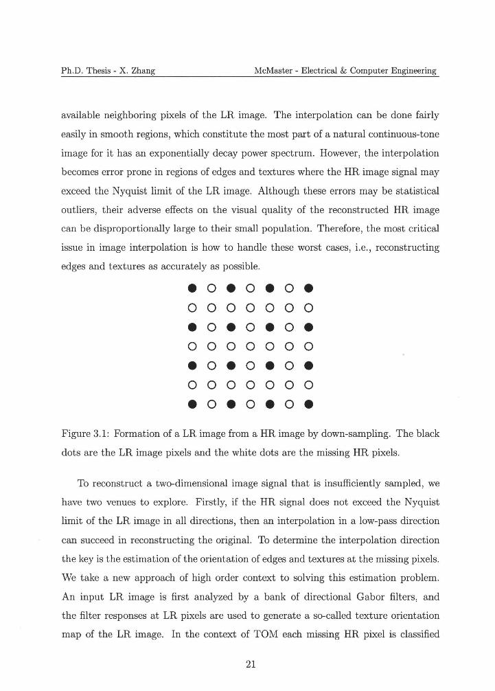
3.1 Formation of a LR image from a HR image by down-sampling. The
black dots are the LR image pixels and the white dots are the missing
HR pixels. . . . . . . . . . . . . . . . . . . . . . . . . . . . . . . . . . 21
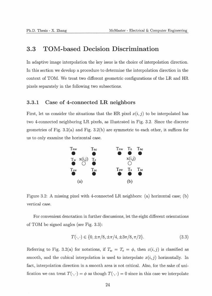
3.2 A missing pixel with 4-connected LR neighbors: (a) horizontal case;
(b) vertical case. . . . . . . . . . . . . . . 24
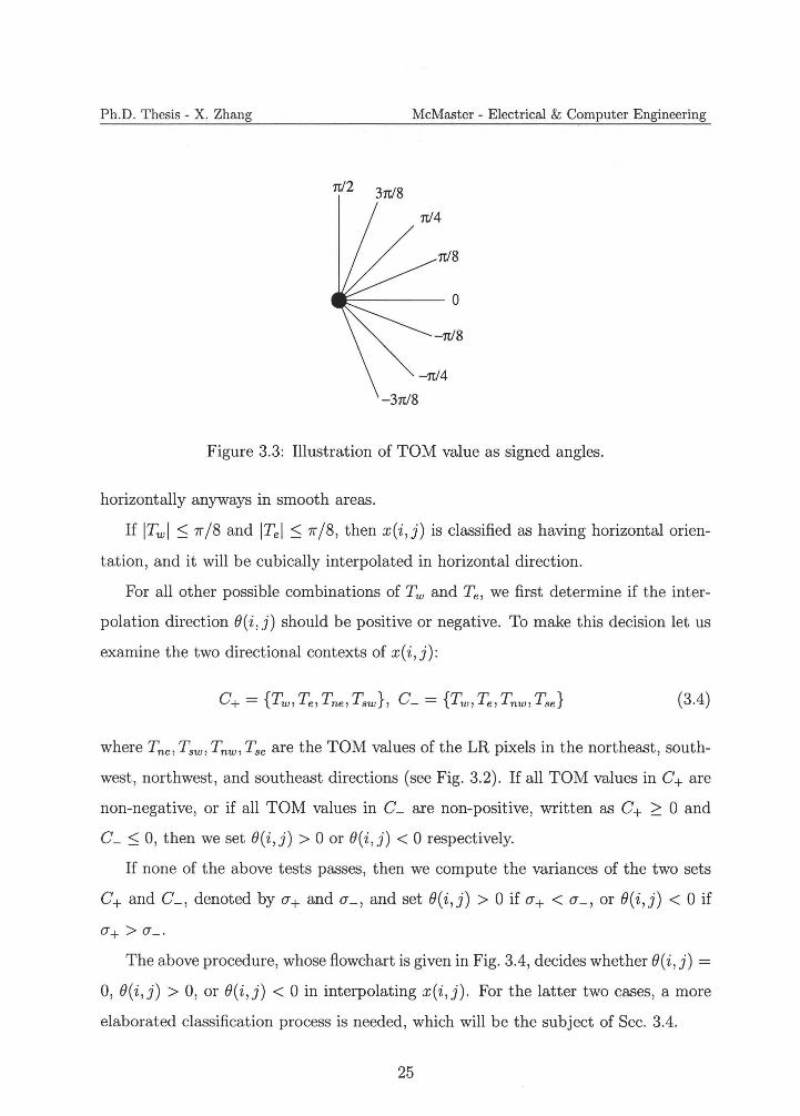
3.3 Illustration of TOM value as signed angles. 25
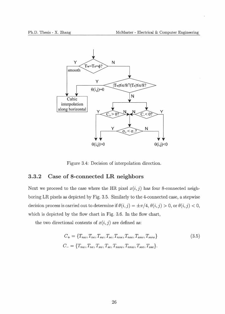
3.4 Decision of interpolation direction. 26
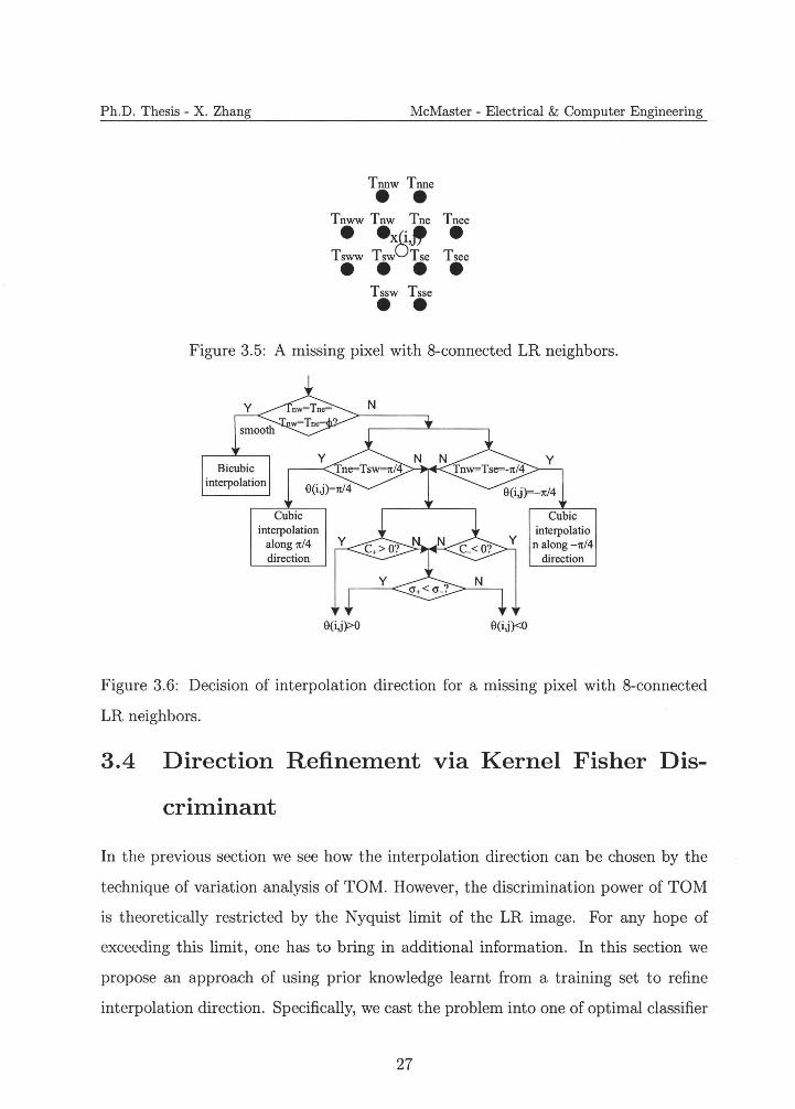
3.5 A missing pixel with 8-connected LR neighbors. 27
3.6 Decision of interpolation direction for a missing pixel with 8-connected
LR neighbors. . . . . . . . . . . . . . . . . . . . . . . . . 27
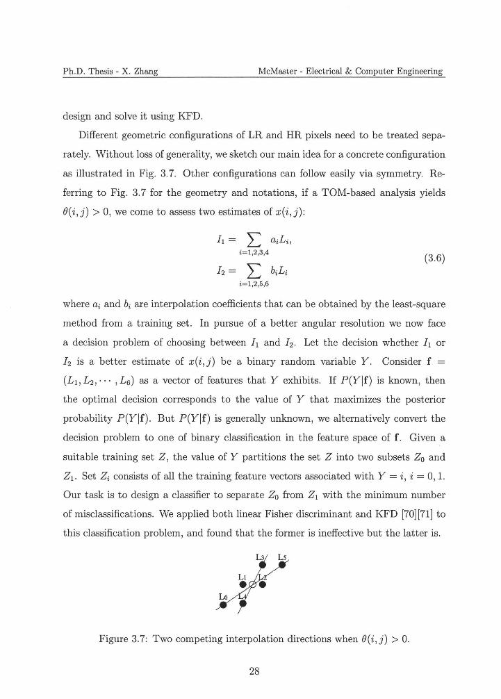
3. 7 Two competing interpolation directions when 0(i, j) > 0. 28
3.8 Reconstructed Baboon images by different methods. . . . 32
Vlll
Ph.D. Thesis - X. Zhang McMaster - Electrical & Computer Engineering
4.1 Formation of a low resolution image from a high resolution image by
down-sampling. The solid black dots are the LR image pixels and the
circles are the missing HR pixels. Interpolation is done in two passes:
The first pass interpolates the missing pixels marked by shaded circles,
and the second pass interpolates the remaining missing pixels marked
by empty circles. . . . . . . . . . . . . . . . . . . . . . . . . . . . . . 37
4.2 (a) Spatial configuration in the first pass. (b) The PAR model parame
ters X = (x1,X2,X3,X4) and 't = (T1,T2,T3,T4) in relationship to spatial
correlations of pixels. . . . . . . . . . . . . . . . . . . . . 38
4.3 Spatial configuration in the second pass of interpolation. 41
4.4 Sample relations in estimating model parameters. . . . . 41
4.5 A possible configuration used in the soft-decision interpolation algorithm 43
4.6 Eight sample images in the test set. . . . . . . . . . . . . . . . . . . . 47
4. 7 Pixel locations where the SAi algorithm has smaller interpolation er
rors than the competing methods (only those of difference 3 or greater
are plotted) on Bike and Lena images. The intensity level represents
the magnitude of reduction in interpolation error by the proposed
method from the competing method. ......... ..... .. 49
4.8 Comparison of different methods on Bike image (to be continued). 52
4.8 Comparison of different methods on Bike image (Cont'd.). . ... 53
4.9 Comparison of different methods on Lena image (to be continued) .. 53
4.9 Comparison of different methods on Lena image (Cont'd.). ..... 54
4.10 Comparison of different methods on Bush image (to be continued). 55
4.10 Comparison of different methods on Bush image (Cont'd .). .. ... 56
4.11 Comparison of different methods on Flower image (to be continued) . . 56
4.11 Comparison of different methods on Flower image (Cont'd .). .... . 57
4.12 Reconstructed images enlarged to compare the edge-directed interpo
lation method and the SAi algorithm (to be continued) ......... 58
IX
Ph.D. Thesis - X. Zhang McMaster - Electrical & Computer Engineering
4.12 Reconstructed images enlarged to compare the edge-directed interpo
lation method and the SAI algorithm (Cont'd.). . . . . . . . . . . . . 59
4.13 Images scaled up by 3 times using different methods: (a) the bicubic
method; (b) the SAi algorithm followed by the bicubic interpolation
(i.e., first scaling by a factor of 2 and then by a factor of 1.5). . . . . 60
4.14 Visual effects of over-fitting of LR data. (a) Original image; (b) The
output image of the SAi algorithm without safe guard against over-
fitting. . . . . . . . . . . . . . . . . . . . . . . . . . . . . . . . . . . . 61
5.1 Sampling relationship between the HR and LR. The scaling factor
shown here is 1.5. The circles are locations of HR pixels and the crosses
are locations of LR pixels. Each LR pixel corresponds to a block of
HR pixels through the filtering operation with a known PSF. 65
5.2 Ten sample images in the test set ............ . .. . 74
5.3 Comparison of different methods on Bush image (to be continued). 79
5.3 Comparison of different methods on Bush image (Cont'd.). . . . . 80
5.4 Comparison of different methods on Hat image (to be continued) . 80
5.4 Comparison of different methods on Hat image (Cont'd.). . . . . . 81
5.5 Comparison of different methods on Lena image (to be continued). . 82
5.5 Comparison of different methods on Lena image (Cont'd.). . . . . . 83
5.6 Comparison of different methods on Flower image (to be continued). . 83
5.6 Comparison of different methods on Flower image (Cont'd.). . . . . . 84
5. 7 Interpolated Bike image with scaling factor a= 1.8 (to be continued) . 85
5.7 Interpolated Bike image with scaling factor a= 1.8 (Cont'd.). . . . . 86
5.8 Interpolated Hat image with scaling factor a = 3.2 (to be continued). 87
5.8 Interpolated Hat image with scaling factor a= 3.2 (Cont'd.). . . . . . 88
5.9 Comparison of different methods on Bike image with scaling factor
a = 4.0 (to be continued). . . . . . . . . . . . . . . . . . . . . . . . . 89
x
Ph.D. Thesis - X. Zhang McMaster - Electrical & Computer Engineering
5.9 Comparison of different methods on Bike image with scaling factor
a= 4.0 (Cont'd.). . . . . . . . . . . . . . . . . . . . . . . . . . . . . . 90
5.10 Effects of changing c in CJ = ca, the standard deviation of a Gaussian
PSF, here a= 1.5. . . . . . . . . . . . . . . . . . . . . . . . . . . 91
6.1 Block diagram of the proposed CADU image compression system. 94
6. 22 Directional filters of maximum passed region WL(B)wH(B) = 11' . 98
6.3 The relationship between the down-sampled pre-filtered image and the
original image. The illustrated kernel size of the filter is 3x3. A low
resolution pixel (black dots in (a)) is the filtered value of the corre
sponding 9 original pixels (white dots in (b)). . . . . . . . . . . . . . 100
6.4 Sample relationships with PAR model parameters: (a) X = (x1, x2 ,x3 , X4) ,
(b) 't = (T1,T2,T3,T4). . . . . . . . . . . . . . . . . . . . . . . . 101
6.5 Comparison of different methods at 0.2bpp (to be continued). 106
6.5 Comparison of different methods at 0.2bpp (to be continued). 108
6.5 Comparison of different methods at 0.2bpp (to be continued). 109
6.5 Comparison of different methods at 0.2bpp (to be continued). 110
6.5 Comparison of different methods at 0.2bpp (to be continued). 111
6.5 Comparison of different methods at 0.2bpp (Cont'd.). . . . . . 112
6.6 Comparison of different methods. Note the superior visual quality of
the CADU method even though it has a lower PSNR (to be continued) . 113
6.6 Comparison of different methods. Note the superior visual quality of
the CADU method even though it has a lower PSNR (Cont'd.). . . . 114
6. 7 Edge-enhanced versions of the output images of JPEG 2000 and CADU
at 0.2bpp. These images are to be compared with their counterparts
in Fig. 6.5 (to be continued). . . . . . . . . . . . . . . . . . . . . . . . 114
6. 7 Edge-enhanced versions of the output images of JPEG 2000 and CAD
Uat 0.2bpp. These images are to be compared with their counterparts
in Fig. 6.5 (Cont'd.) . . . . . . . . . . . . . . . . . . . . . . . . . . . . 115
Xl
Ph.D. Thesis - X. Zhang McMaster - Electrical & Computer Engineering
7.1 SMMD Framework. . . . . . . . . . . . . . . . 118
7.2 Block diagram of the SMMD central decoder. 119
7.3 The relationship between low-resolution pixel Yi with its neighbors in
jQ· . . . . . . . . . . . . . . . . . . . . . . . . . . . . . . . . . . . . . 121
7.4 Comparison of different methods in both side and central PSNR (dB)
versus the central rate (bpp) (to be continued) . . . . . . . . . . . . . 123
7.4 Comparison of different methods in both side and central PSNR (dB)
versus the central rate (bpp) (Cont'd.). . . . . . . . . . . . . . . . . . 124
7.5 Comparison of decoded Lena images at 0.25 bpp/description (to be
continued). . . . . . . . . . . . . . . . . . . . . . . . . . . . . . . . . 125
7.5 Comparison of decoded Lena images at 0.25 bpp/description (Cont'd.). 126
7.6 Comparison of decoded Fruit images at 0.4 bpp/description (to be
continued). . . . . . . . . . . . . . . . . . . . . . . . . . . . . . . . . 126
7.6 Comparison of decoded Fruit images at 0.4 bpp/description (Cont'd.). 127
7.7 Comparison of decoded Bike images at 0.6 bpp/description. Note that
the SMMD side decoder produces superior visual quality even though
it has lower PSNR than the other two MDC techniques. . . . . . . . . 128
7.8 Comparison of the performance of SMMD central decoder and side
decoder. . . . . . . . . . . . . . . . . . . . . . . . . . . . . . . . . . . 129
Xll
List of Tables
3.1 The PSNR(dB) results . . . . . . . . . . . . . . . . . . . . . . . . . . 31
4.1 PSNR (dB) results of the reconstructed HR images by different meth
ods. The number in parentheses is the rank of the method. For the
SAi algorithm, its gain in dB over the second best method is also given. 48
5.1 PSNR (dB) of reconstructed HR images by different methods. For the
first four methods the results with and without Wiener deconvolution
are included. . . . . . . . . . . . . . . . . . . . . 76
6.1 The design of directional low-pass 2D pre-filters 97
6.2 The PSNR (dB) results for different compression methods. 104
Xlll
List of Abbreviations
2D
AR
ARMA
bpp
CADU
CADU-JPG
CADU-J2K
CALIC
CCD
CMOS
dB
DCT
dpi
FIR
HR
JPEG
JPEG 2000
KFD
LR
Two-dimension
Autoregressive
Autoregressive moving average
bit per pixel
Collaborative adaptive down-sampling and upconversion
CADU method coupled with DCT-based JPEG
CADU method coupled with JPEG 2000
Context-based adaptive lossless codec [1]
Charged couple device
Multiple Description Lattice Vector Quantization
Decibel
Discrete cosine transform
Dot per inch
Finite impulse response
High resolution
Joint photographic experts group
A compression standard by JPEG [2]
Kernel fisher discriminant
Low resolution
XIV
Ph.D. Thesis - X. Zhang McMaster - Electrical & Computer Engineering
MA
MD
MDC
MMSE
NEDI
NEARU
PAR
POCS
PSF
PSNR
SAi
SMMD
SNR
STLS
TMW
TOM
Moving average
Multiple description
Multiple description coding
Minimum mean square error
New edge directed interpolation [3]
Non-linear estimation for adaptive resolution upconversion
Piecewise autoregressive
Projection onto convex sets
Point spread function
Peak signal-to-noise ratio
Soft-decision adaptive interpolation
Spatial multiplexing multiple description
Signal-to-noise ratio
Structure total least square
A lossless compression method in [4]
Texture orientation map
xv
Ph.D. Thesis - X. Zhang McMaster - Electrical & Computer Engineering
Chapter 1
Introduction
1.1 The Problem and Motivation
Digital images have, in both still and moving forms, become a main medium of
information, knowledge, and communication in our modern technology era. People
in all walks of life now truly appreciate the connotation of the old saying "a picture is
worth a thousand words". Many may find digital images/videos too informative, too
convenient, too timely and too rich to do without. Compared to their counterparts
on paper and film, digital images are vastly more convenient and inexpensive to
generate, communicate, process, store and retrieve. With intensive research and
heavy investment in sensor technologies, the spatial resolution and color fidelity of
digital images are steadily improving and now can match those of traditional film.
One of the most important quality metrics of digital images is and will continue to
be the spatial resolution. High spatial resolution is necessary to reveal fine structural
information on the imaged objects and scenes. High resolution directly translates
to high precision in computerized image analysis, which is paramount in medical,
scientific and military applications. Even in consumer electronics, entertainment in
dustry, and other commercial applications, users desire high image resolution because
resolution is in general proportional to perceived image quality. To appreciate this
1
Ph.D. Thesis - X. Zhang McMaster - Electrical & Computer Engineering
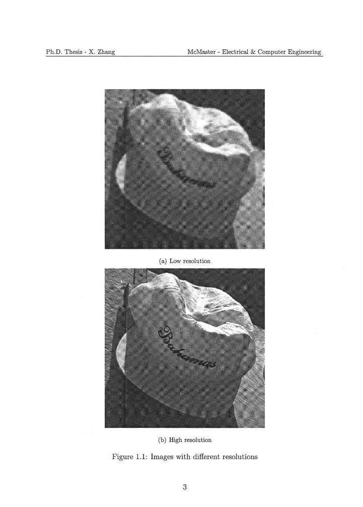
the reader is invited to compare two images of the same scene but of different spatial
resolutions in Fig. 1.1.
In an ideal world, one can always increase the sensor resolution of image acquisition
devices to obtain a desired spatial resolution. However, several limiting factors nullify
this approach. First, the cost of image sensors increases drastically in resolution. For
instance, in today's consumer market, digital cameras of ten million pixels typically
cost more than twice as much as those of seven million pixels. Second, there exist
hard physical limits on how high a spatial resolution that an imaging device can
achieve. Most digital images are acquired by an array of semiconductor sensors such as
charged couple device (CCD) or complementary metal-oxide-semiconductor (CMOS).
Ultra-high spatial resolution means that the size of pixel (i.e., the cross section of a
sensor area) diminishes. However, the signal-to-noise ratio (SNR) of the acquired
image is proportional to its size [5]. Too small a pixel will render an image useless
due to insufficient SNR. Moreover, electronic interferences are inevitable between
neighboring sensors. The closer the neighboring sensors are, the larger the interference
become. Therefore, given an SNR requirement, either the size of the sensor or the
distance between neighboring sensors can not be below a hard threshold. Third, in
some cases the imaging process itself incurs a penalty to the imaged object, which
limits the number of samples (pixels) to be acquired. For example, for certain medical
imaging technologies, high resolution is associated with large dosage of radiation that
is harmful to the patient. Finally, no matter how high the native sensor resolution
of an imaging device is, new, more exciting or more exotic applications will always
present themselves that demand even higher spatial resolution. As one can imagine,
researchers in medicine, space, and sciences all have insatiable appetite for imaging
ever more minuscule details. This is even the case for more mundane application of
digital photo finishing. Nowadays the resolution of photo printers can be 2400 dot
per inch (dpi) or higher. Even for inexpensive home printers of a resolution of 1200
dpi, a photo print of size 4 inch by 6 inch contains 4 x 1200 x 6 x 1200 = 34 million
2
Ph.D. Thesis - X. Zhang McMaster - Electrical & Computer Engineering
(a) Low resolution
(b) High resolution
Figure 1.1: Images with different resolutions
3
Ph.D. Thesis - X. Zhang McMaster - Electrical & Computer Engineering
pixels, which far exceeds the resolution of even most expensive professional digital
cameras.
Image interpolation, or image resolution upconversion, is a technology to improve
the native sensor resolution by reconstructing an image of higher resolution from a
lower resolution version. Interpolation of a discrete signal is a classic problem in
applied mathematics and signal processing. The goal is to reconstruct a continuous
function from a set of discrete data (samples). A digital signal is typically generated
by sampling the corresponding continuous signal in space or time. A digital image of
different resolutions corresponds to different sampling schemes of the same continuous
signal. To increase the resolution, the interpolation is performed to estimate the
continuous image signal from the observed low resolution image. The high resolution
image can then be obtained by re-sampling the continuous image signal. In this
thesis, we focus on the interpolation problem of recovering a high resolution (HR)
image from its associated low resolution (LR) image.
The challenge to image interpolation is the reconstruction of high frequency com
ponents of an image, such as edges and fine textures. Low frequency components of an
HR image can be recovered from a corresponding LR image more easily than the high
frequency components. According to Nyquist sampling theory [6], only those compo
nents that have frequency below the Nyquist frequency can be exactly reconstructed.
All interpolation methods can do a comparable good job in reconstructing smooth
two-dimension (2D) waveforms. It is the interpolation accuracy on spatial structures
of high frequency that differentiates the good image interpolation methods from the
poor ones. Inferior interpolation methods are prone to artifacts in the areas of edges
and fine textures. The common visual defects due to interpolation errors are blurred
or/and jaggy edges and aliasing. To aggravate the difficulty of reconstructing edges,
the human vision system is highly sensitive to noises accompanying edges. This is
because edges convey much of the image semantics. Edges signify vital attributes of
an object such as shape, size, and surface characteristics, as well as spatial relation
4
Ph.D. Thesis - X. Zhang McMaster - Electrical & Computer Engineering
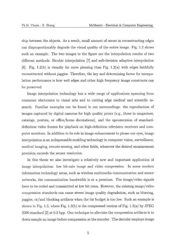
ship between the objects. As a result, small amount of errors in reconstructing edges
can disproportionably degrade the visual quality of the entire image. Fig. 1.2 shows
such an example. The two images in the figure are the interpolation results of two
different methods: Bicubic interpolation [7] and soft-decision adaptive interpolation
[8] . Fig. 1.2(b) is visually far more pleasing than Fig. 1.2(a) with edges faithfully
reconstructed without jaggies. Therefore, the key and determining factor for interpo
lation performance is how well edges and other high frequency image constructs can
be preserved.
Image interpolation technology has a wide range of applications spanning from
consumer electronics to visual arts and to cutting edge medical and scientific re
search. Familiar examples can be found in our surroundings: the reproduction of
images captured by digital cameras for high quality prints (e.g., those in magazines,
catalogs, posters, or office/home decorations), and the upconversion of standard
definition video frames for playback on high-definition television receivers and com
puter monitors. In addition to its role in image enhancement to please our eyes, image
interpolation is an indispensable enabling technology in computer vision, surveillance,
medical imaging, remote sensing, and other fields, whenever the desired measurement
precision exceeds the sensor resolution.
In this thesis we also investigate a relatively new and important application of
image interpolation: low bit-rate image and video compression. In some modern
information technology areas, such as wireless multimedia communication and sensor
networks, the communication bandwidth is at a premium. The image/video signals
have to be coded and transmitted at low bit rates. However, the existing image/video
compression standards can cause severe image quality degradation, such as blurring,
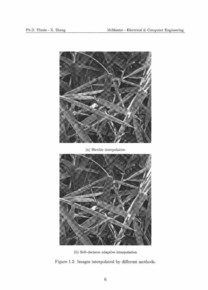
jaggies, or/and blocking artifacts when the bit budget is too low. Such an example is
shown in Fig. 1.3, where Fig. 1.3(b) is the compressed version of Fig. 1.3(a) by JPEG
2000 standard [2] at 0.2 bpp. One technique to alleviate the compression artifacts is to
down sample an image before compression at the encoder. The decoder employs image
5
Ph.D. Thesis - X. Zhang McMaster - Electrical & Computer Engineering
(a) Bicubic interpolation
(b) Soft-decision adaptive interpolation
Figure 1.2: Images interpolated by different methods.
6
Ph.D. Thesis - X. Zhang McMaster - Electrical & Computer Engineering
(a) Original image
(b) Compressed by JPEG 2000
Figure 1.3: Original image and the compressed version at 0.2 bpp.
7
Ph.D. Thesis - X. Zhang McMaster - Electrical & Computer Engineering
interpolation to upconvert the decompressed image back to the original resolution.
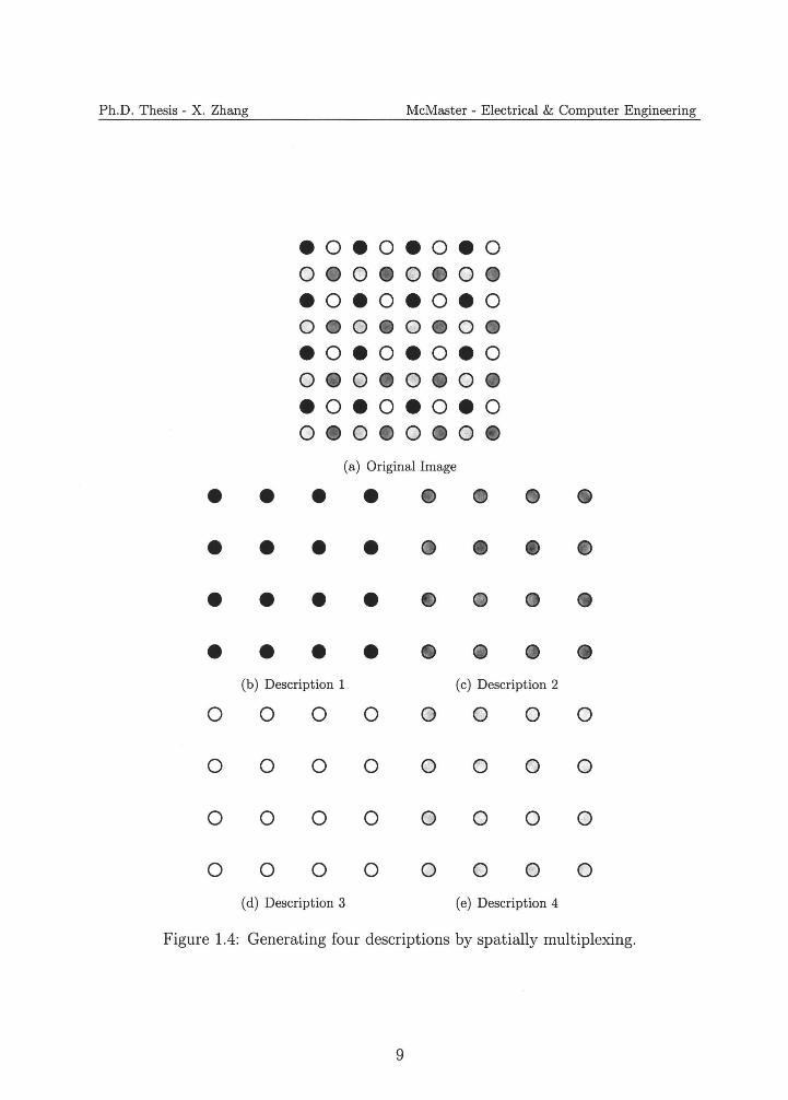
Image interpolation can also be used as a technique for multiple description cod
ing (MDC) of images. MDC is an effective methodology for signal communication
over unreliable diversity channels, to which a great deal of research efforts have been
devoted in the past decade. In image MDC an input image is encoded into several bit
streams or multiple descriptions and transmitted through independent lossy channels.
The decoder can reconstruct the original image if any subset of the transmitted de
scriptions can be received. The more descriptions arrive at the decoder, the higher the
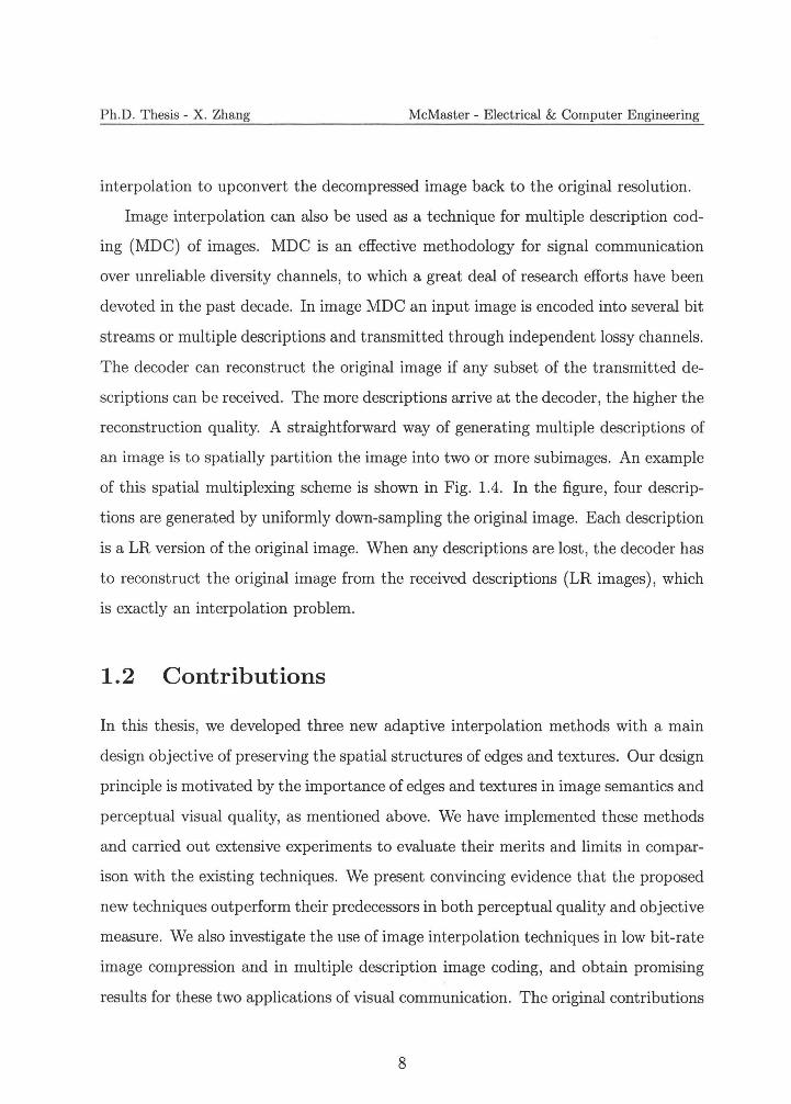
reconstruction quality. A straightforward way of generating multiple descriptions of
an image is to spatially partition the image into two or more subimages. An example
of this spatial multiplexing scheme is shown in Fig. 1.4. In the figure, four descrip
tions are generated by uniformly down-sampling the original image. Each description
is a LR version of the original image. When any descriptions are lost, the decoder has
to reconstruct the original image from the received descriptions (LR images), which
is exactly an interpolation problem.
1.2 Contributions
In this thesis, we developed three new adaptive interpolation methods with a main
design objective of preserving the spatial structures of edges and textures. Our design
principle is motivated by the importance of edges and textures in image semantics and
perceptual visual quality, as mentioned above. We have implemented these methods
and carried out extensive experiments to evaluate their merits and limits in compar
ison with the existing techniques. We present convincing evidence that the proposed
new techniques outperform their predecessors in both perceptual quality and objective
measure. We also investigate the use of image interpolation techniques in low bit-rate
image compression and in multiple description image coding, and obtain promising
results for these two applications of visual communication. The original contributions
8
Ph.D. Thesis - X. Zhang McMaster - Electrical & Computer Engineering
eoeoeoeo o • o • o • o • •o•o•o•o o e o e o e o e eoeoeoeo o e o • o • o • eoeoeoeo o • o • o • o •
(a) Original Image
• • • • • • • • • • • • • • • • • • • • • • • • • • • • • • • •
(b) Description 1 (c) Description 2
0 0 0 0 0 0 0 0
0 0 0 0 0 0 0 0
0 0 0 0 0 0 0 0
0 0 0 0 0 0 0 0
(d) Description 3 (e) Description 4
Figure 1.4: Generating four descriptions by spatially multiplexing.
9
Ph.D. Thesis - X. Zhang McMaster - Electrical & Computer Engineering
of this thesis are summarized as follows.
• A new adaptive non-linear image interpolation approach is proposed that chooses
an interpolation direction based on contextual information of the LR image.
The selection of the best interpolation direction among all possible candidate
directions is converted to a classification problem. The classifier is designed us
ing a training set of HR images. This new classification-based method achieves
higher peak signal-to-noise ratio (PSNR) and better visual quality than previ
ous methods. It can correctly solve some of the very difficult cases for which
the traditional methods fail.
• Our second new image interpolation technique is called soft-decision adaptive
interpolation (SAI). The SAI technique learns and adapts to varying scene struc
tures using a 2D piecewise autoregressive model. The model parameters are
estimated in a moving window in the input low resolution image. And the pixel
structure dictated by the learnt model is enforced by the soft-decision estima
tion process onto a block of HR pixels, including both observed and estimated.
This new image interpolation technique produces some of the best results so far
by preserving spatial coherence of interpolated images better than the existing
methods.
• Our third new, the most sophisticated image interpolation technique is a model
based non-linear image restoration scheme. The task of image resolution upcon
version is formulated as a problem of adaptive piecewise autoregressive modeling
and estimation, where the model parameters and the HR pixels are jointly es
timated through non-linear least squares estimation. The new method offers
a unified general framework for image upsampling and deconvolution, and the
upsampling can be carried out at an arbitrary scale. The method outperforms
convincingly the current methods in both PSNR and subjective visual quality,
and its advantage becomes greater for larger scaling factors.
10
Ph.D. Thesis - X. Zhang McMaster - Electrical & Computer Engineering
• We investigate the use of image interpolation as a technique for low bit-rate
image compression, and propose a collaborative adaptive down-sampling and
upconversion ( CADU) approach to image compression. In this approach, the
input images are adaptively prefiltered, uniformly down sampled, and com
pressed at the encoder. The decoder upconverts the decoded LR images to the
original resolution in a constrained least squares restoration process, using a
2D piecewise autoregressive model and the knowledge of directional low-pass
prefiltering. The CADU approach achieves the highest PSNR and best visual
quality up to now for low bit rates, and it is completely compatible with any
existing compression standards.
• We are among the first to study the application of image interpolation in multi
ple description image coding. Our contribution to this new subject is a spatial
multiplexing multiple description (SMMD) scheme. Multiple descriptions of an
image are generated in the spatial domain by an adaptive prefiltering and uni
form down sampling process. The resulting side descriptions are conventional
square sample grids and can be coded by any of the existing image compression
methods. The side decoder and central decoder reconstruct the input image by
first decompressing the down-sampled image and then solving a least-squares
inverse problem, guided by a 2D piecewise autoregressive model. Compared
with the existing image MDC methods in the literatures, the proposed SMMD
technique offers the lowest encoder complexity, complete standard compliance,
competitive rate-distortion performance, and superior subjective quality.
These contributions are contained in the remaining chapters of this thesis as well as
four conference and three journal papers. Our first new adaptive interpolation method
was presented in IEEE !GIP 2005 [9]. The second method, SAI, was published in
IEEE Transactions on Image Processing [8] . An earlier exposition of this method was
presented in IEEE !GIP 2007 [10]. Our third interpolation method, the model-based
nonlinear image restoration scheme, was submitted to IEEE Transactions on Image
11
Ph.D. Thesis - X. Zhang McMaster - Electrical & Computer Engineering
Processing for review [11]. The CADU technique for low-rate image compression
was presented in IEEE DCC 2008 [12], and a journal paper will appear in IEEE
Transactions on Image Processing [13]. The SMMD scheme was presented in IEEE
MMSP 2008 [14].
1.3 Organization
The remaining of this thesis is organized as follows. Chapter 2 reviews existing
works on image interpolation and the interpolation based low-rate image compression
methods. Our first adaptive non-linear image interpolation method is described in
Chapter 3. Chapter 4 presents the new soft-decision adaptive image interpolation
method. Our most sophisticated interpolation technique, the model-based nonlinear
image restoration scheme, is proposed in Chapter 5. Chapter 6 develops the CADU
approach for low bit-rate image compression, and the SMMD scheme is studied in
Chapter 7. The thesis closes with conclusions and suggested future works in Chapter
8.
12
Ph.D. Thesis - X. Zhang McMaster - Electrical & Computer Engineering
Chapter 2
Review of Existing Works
Interpolation as a topic of mathematics has a very long history. A chronological
overview of the developments in interpolation theory since ancient time was presented
in [15]. The first application of interpolation in image processing was reported in
early 1970s. From then, many image interpolation techniques have been developed.
Depending on whether they are adaptive to the image signals, these techniques can
be classified in two groups: non-adaptive methods and adaptive methods. The non
adaptive image interpolation methods have the advantages of low complexity and
low cost of hardware implementation. Their common drawback is the inability to
adapt to varying pixel structures in a scene, due to the use of scene-independent
interpolators. As a result, they are all susceptible to defects such as jaggies, blurring,
and ringing. The adaptive interpolation methods generally have higher interpolation
accuracy or/and better visual quality in the expense of higher computation complexity
than the non-adaptive methods. In this chapter, we will review some representative
and popular image interpolation algorithms in both groups, as well as some existing
interpolation based low-rate image compression methods.
13
Ph.D. Thesis - X. Zhang McMaster - Electrical & Computer Engineering
2.1 Non-adaptive Interpolation Methods
The simplest interpolation methods are nearest neighbor interpolation and bilinear
interpolation [16] . Nearest neighbor interpolation simply duplicates the nearest pixel
for each missing pixel in the high resolution image. Bilinear interpolation is also very
simple. It reconstructs a missing pixel as an average of its neighboring low resolution
pixels. These two methods are very fast, but their performance leaves much to be
desired. Nearest neighbor interpolation produces objectionable checkerboard effect,
particularly for large scaling factors; and bilinear interpolation severely blurs edges
and textures.
More complicated methods were developed to improve the interpolation accuracy.
One popular technique is cubic convolution. It uses a sine-like kernel composed of
piecewise cubic polynomials and significantly improves the interpolation accuracy of
the nearest neighbor and bilinear interpolation methods. Cubic convolution tech
nique was first mentioned in the early 1970s and was analyzed in detail by Keys [7]
in 1981 for digital image interpolation. The technique was also examined by Park
and Schowengerdt in frequency domain [17]. The cubic convolution interpolation is
also known as bicubic interpolation when applied to images since it interpolates pix
els in two separate directions: horizontal and vertical. Motivated by the statistical
nonseparable property of real natural images, nonseparable 2D interpolation filters
were designed [18, 19, 20]. In [19], Reichenbach and Geng derived a 2D nonseparable
cubic convolution kernel with two parameters and showed that it produced higher
interpolation accuracy than separable cubic convolution. Later, Shi and Reichenbach
relaxed the constraints in [19] and derived another two nonseparable cubic convolu
tion kernels with three and five parameters respectively, and improved somewhat on
the interpolation accuracy [20]. The improvements made by the non-separable 2D
interpolation kernels were obtained at the expense of higher complexity.
Splines were also used in image interpolation. The earliest and popular method
was developed by Hou and Andrews in 1978 [21] . The method is known as B-spline
14
Ph.D. Thesis - X. Zhang McMaster - Electrical & Computer Engineering
interpolation or cubic spline interpolation. Maeland compared the cubic spline in
terpolation with cubic convolution interpolation, and concluded that cubic spline
interpolation had superior performance but higher complexity [22]. Unser et al. de
signed an optimal spline algorithm and claimed that the method could achieve the
closest approximation of the original signal in the Lrnorm [23]. The splines were
also thoroughly studied as an effective tool for signal and image processing in [24].
To reduce the complexity, Vrcelj and Vaidyanathan replaced the B-Spline filter with
a short finite impulse response (FIR) filter and proposed a simplified implementation
of the B-splines based image interpolation methods [25].
Besides cubic convolution and cubic splines, many other kernels were proposed for
image interpolation. Some of these kernels were described and compared by Lehmann
and Spizter in [26]. In particular, they analyzed B-spline interpolation techniques of
degree 2, 4, and 5 in [27]. They concluded that high-degree B-splines had higher
interpolation accuracy and comparable complexity compared with lower degree B
splines.
2.2 Adaptive Interpolation Methods
With ever increasing computation power in image and video processing, more so
phisticated adaptive image interpolation methods were proposed to improve the non
adaptive interpolation methods.
To adapt interpolators to local properties of images, many researchers proposed
modifications on conventional cubic convolution interpolation and cubic spline inter
polation methods [28, 29, 30, 31]. In [28], Ramponi proposed a warped distance-based
adaptive image interpolation method. The main idea of this method is to modify the
Euclidean distances to reflect some local property of the image signal. This method
can be easily combined with conventional image interpolation methods such as bilin
ear, bicubic, or cubic spline interpolation. Han and Baek [29] adaptively modified the
15
Ph.D. Thesis - X. Zhang McMaster - Electrical & Computer Engineering
parametes of the parametric cubic convolution kernel and reported better results than
traditional bicubic method. In [30], Shi and Ward proposed a postprocessing method
to improve the visual quality of the interpolated images. The values of pixels near
edges were modified to reduce jaggies caused by non-adaptive interpolation methods.
Hwang and Lee applied an inverse gradient to the structure of conventional bilinear
and bicubic interpolation to sharpen edges[31]. In [32], the authors applied splines
as image model to interpolate the high resolution images from nonuniformly sampled
images. The interpolation problem was formulated in spline domain and an adaptive
smoothness prior was used as regularization term.
As discussed in the previous chapter, edges play important role in human vision
system. Non-adaptive interpolation methods tend to blur edges and/or introduce
artifacts in edge area due to their isotropic interpolation kernels. In fact, edges have
asymmetric spectrum since the frequency is low along edges and high perpendicular
to edges. To exploit this property, many researchers advocated the approach of edge
guided interpolation. Jensen and Anastassiou published a scheme that detects edges
and fits them with some templates to improve the visual perception of interpolated
images [33]. Allebach and Wong detected the edges of the original image first and then
used the generated edge map to emphasize the visual integrity of the detected edges
[34]. Method in [35] first estimated the local characteristics of the image by performing
block classification and then applied different filters to reconstruct the high resolution
images. Carrato and Tenze used some predetermined edge patterns to optimize the
parameters in the interpolation operator [36]. Malgouyres and Guichard theoretically
and experimentally analyzed some edge-guided image enlargement methods in [37].
In [38], an edge-directed interpolation method was proposed with emphasizing on the
fidelity and sharpness of edges in the interpolated images. In [39], Muresan proposed
a fast edge-directed polynomial interpolation method. Edge pixels were interpolated
along the edge direction, and non-edge pixels were interpolated by fusing the multi
directional estimates. Wang and Ward [40] detected step edges or ridges, and then
16
Ph.D. Thesis - X. Zhang McMaster - Electrical & Computer Engineering
applied bilinear method with an orientation-adaptive parallelogram to reconstruct
the missing high resolution pixels on those edges or ridges.
Instead of explicitly detecting edges prior to interpolation, many edge-guided in
terpolation methods rely on implicit edge information. Li and Orchard proposed to
estimate the covariance of high resolution image from the covariance of the low resolu
tion image, and then interpolate the missing pixels based on the estimated covariance
[3]. Since the edge information is built into the algorithm, the method preserves
edge structures well. This edge-directed interpolation work was cast by Muresan and
Parks into the framework of adaptive optimal recovery [41]. Alternatively, Zhang and
Wu proposed to interpolate a missing pixel in multiple directions, and then fuse the
directional interpolation results by minimum mean square error (MMSE) estimation
[42]. Also, Cha and Kim proposed a postprocessing method to estimate the high
resolution image based on a system of nonconvex nonlinear partial differential equa
tions [43]. They reported that clear edges were formed after 2 to 3 iterations. They
further extended the method to interpolate color images where the three channels
were jointly interpolated [44]. Another edge-guided method was proposed in [45].
In this method, the edge directions were implicitly estimated and were indicated by
length-16 weighting vectors, and these weighting vectors were implicitly used to for
mulate geometric regularity constraint which was imposed on the interpolated image
through a Markov random field model.
Wavelets were also used in image interpolation. The interpolation is done by pre
dicting the high-resolution details from the low resolution observations [46, 47, 48,
49, 50]. Carey et al. proposed a method that estimated the regularity of edges by
measuring the decay of wavelet transform coefficients across scales and preserved the
underlying regularity by extrapolating a new subband to be used in image resynthesis
[46]. In [47], an MMSE estimator was constructed to synthesize the detailed wavelet
coefficients as well as to minimize the mean squared error for high-resolution signal
recovery. Based on the behavior of edges across scales in the scale-space domain,
17
Ph.D. Thesis - X. Zhang McMaster - Electrical & Computer Engineering
Muresan and Parks estimated the coefficients of the fine scale from a set of known
coefficients at the coarser scales [48]. Chang and Cvetkovic used the wavelet trans
form to extract information about sharp variations in the low resolution images, and
then implicitly applied interpolation that adapts to the image local characteristics
[49]. In [50], Temizel and Vlachos exploited wavelet coefficient correlation in a local
neighborhood and employed linear least-squares regression to estimate the unknown
detail coefficients.
The problem of image interpolation has been also studied in the field of the com
puter vision [51, 52, 53, 54, 55]. In [51], a set of deformable contours were used to
define the boundaries between regions in an image and were evolved by a gradient
flow. The goal of the interpolation in this method is to smooth the boundaries while
maintain sharp transitions across region boundaries. Freeman et al. [52] selected
high-resolution patches from training set according to local low-frequency details and
adjacent, previously determined high-frequency patches. Similar method was further
developed in [53] and [54]. In [53], Baker and Kanada focused on the reconstruction
of high-resolution face images from training set. Sun et al. [54] first detected the
contours of the objects and then reconstructed high resolution image primitives along
contours from the training set. In this method, contour smoothness constraints were
also enforced by a Markov chain based inference algorithm. In [55], Lin et al. classi
fied the image into human perception nonsensitive class and sensitive class according
to the characteristics of the human vision system. A trained neural network was used
to interpolate the sensitive region along the edge directions.
Other techniques were also developed for image interpolation. In [56], the image
was modeled as a Markov random field, and the high resolution image was estimated
by maximum a posterior estimation. Iterative methods, such as projection onto
convex sets (POCS) schemes [57, 58], were also proposed for image interpolation.
Fekri et al. applied vector quantization method to the interpolation of text images
[59]. Woods et al. [60] proposed algorithms for reconstructing high resolution image
18
Ph.D. Thesis - X. Zhang McMaster - Electrical & Computer Engineering
from multiple low resolution images. The authors developed two algorithms based
on the expectation maximization and maximum a posteriori respectively. In [61], a
kernel function was added in the regression to give the nearby samples higher weight
than samples farther away when estimating parameters in the regression function. In
[62] , Kopf et al. used bilateral filters to reconstruct a better high resolution image
from the available high resolution image and the associated low resolution image.
2.3 Interpolation Based Low-Rate Image Compres
sion Methods
In this section, we will review interpolation based low-rate image compression meth
ods. In these methods, the input image is downsampled before compression, and the
decoder applies image interpolation methods to upconvert the LR image to original
resolution. Such a scheme first appeared in literature in 1993 [63], and was further
studied by some researchers in recent years [64, 65, 66, 67, 68]. In [64] Bruckstein et al.
explained analytically why it is advantageous to downsample an image prior to JPEG
compression and then upsample the JPEG-decoded image. The authors developed a
model for expected distortion of discrete cosine transform (DCT) based JPEG codec
and gave an expression to determine the rate-distortion optimal downsampling factor.
Segall et al. extended the interpolation based compression scheme to low-rate video
coding [65]. Following up on [64], Tsaig et al. proposed an image-dependent algorithm
to find optimal filters for decimation and interpolation [66] . Lin and Dong studied
the so-called critical bit rate, below which it pays to downsample an image prior to
DCT-based JPEG compression [67]. In addition they proposed a downsampling tech
nique that adapts downsampling factor, direction and DCT quantization step size to
local image characteristics. Gan et al. also proposed undersampled boundary pre
and post-filters to subdue blocking artifacts of DCT-based block codecs at low bit
rates [68].
19
Ph.D. Thesis - X. Zhang McMaster - Electrical & Computer Engineering
Chapter 3
Method of Texture Orientation
Map and Kernel Fisher
Discriminant
In this chapter we present our first new adaptive non-linear image interpolation
method. In this method, a texture orientation map (TOM) of the LR image is
generated by directional Gabor filters to estimate the edge directions. The interpo
lation direction for each missing HR pixel is determined initially by TOM in a local
window, and is then refined by a kernel Fisher discriminant. This allows the interpo
lator to exploit prior knowledge gained from a training set. After the interpolation
direction is determined, the missing HR pixels are estimated by interpolating along
that direction.
3 .1 Overview
As in the exiting literature, we model a LR image as a down-sampled version of the
associated HR image, as illustrated in Fig. 3.1. The task of image interpolation is to
estimate the values of those pixels that are missing in the HR image based on the
20
Ph.D. Thesis - X. Zhang McMaster - Electrical & Computer Engineering
available neighboring pixels of the LR image. The interpolation can be done fairly
easily in smooth regions, which constitute the most part of a natural continuous-tone
image for it has an exponentially decay power spectrum. However, the interpolation
becomes error prone in regions of edges and textures where the HR image signal may
exceed the Nyquist limit of the LR image. Although these errors may be statistical
outliers, their adverse effects on the visual quality of the reconstructed HR image
can be disproportionally large to their small population. Therefore, the most critical
issue in image interpolation is how to handle these worst cases, i.e., reconstructing
edges and textures as accurately as possible.
• 0 • 0 • 0 • 0 0 0 0 0 0 0
• 0 • 0 • 0 • 0 0 0 0 0 0 0
• 0 • 0 • 0 • 0 0 0 0 0 0 0
• 0 • 0 • 0 • Figure 3.1 : Formation of a LR image from a HR image by down-sampling. The black
dots are the LR image pixels and the white dots are the missing HR pixels.
To reconstruct a two-dimensional image signal that is insufficiently sampled, we
have two venues to explore. Firstly, if the HR signal does not exceed the Nyquist
limit of the LR image in all directions, then an interpolation in a low-pass direction
can succeed in reconstructing the original. To determine the interpolation direction
the key is the estimation of the orientation of edges and textures at the missing pixels.
We take a new approach of high order context to solving this estimation problem.
An input LR image is first analyzed by a bank of directional Gabor filters, and
the filter responses at LR pixels are used to generate a so-called texture orientation
map of the LR image. In the context of TOM each missing HR pixel is classified
21
Ph.D. Thesis - X. Zhang McMaster - Electrical & Computer Engineering
either as smooth or textural. In smooth regions the interpolation can be done by
any existing method. For the textural pixels the interpolation direction is carefully
chosen by examining TOM in local windows of different orientations and measuring
the directional variations.
Secondly, even if the HR signal is beyond the Nyquist limit in all directions, we
can still hope for good estimate of the missing samples by using some suitable prior
knowledge. One possibility is to use training data to learn edge/ texture orientation
hence the correct interpolation direction in a context of TOM of the LR image. We
cast the determination of correct interpolation direction into an optimal classifica
tion problem, in which the observable features fed to the classifier are drawn from
TOM. The technique of kernel Fisher discriminant (KFD) is used to design the classi
fier. This classification-driven interpolation technique is able to resolve some of very
difficult cases for which the existing methods fail.
This chapter is organized as follows. The texture orientation map is defined in
Sec. 3.2, followed by discussions on how to use TOM to estimate interpolation direc
tions in Sec. 3.3. Sec. 3.4 develops the kernel Fisher discriminant technique to refine
the interpolation directions using prior knowledge of a training set. Sec. 3.5 reports
experimental results. This chapter closes with a summary in Sec. 3.6.
3.2 Texture Orientation Map
Adaptive directional interpolation in reconstructing a HR image needs to be anchored
on contextual information from the observed LR image. To this end we build a so
called texture orientation map that presents the texture orientation of each pixel in
the LR image. A bank of Gabor filters is applied to detect the presence or lack of
an edge at each LR pixel, and determine the direction of the edge, if it exists. We
22
Ph.D. Thesis - X. Zhang McMaster - Electrical & Computer Engineering
choose the following bank of Gabor filters:
im = icos(Om) + jsin(Om); (3.1)
jm = -isin(Om) + jcos(Om);
(m - l)7rOm= ; m=l,2, ... ,8
8
where <Ji and <7j are standard deviations of the Gaussian envelope, and f is the fre
quency of the sinusoid. Although filters of arbitrary orientations are analytically
possible, we use only eight uniformly quantized discrete orientations for ease of im
plementation and because such an angular resolution is sufficient for an expansion
factor of two from LR image to HR image (see Fig. 3.1). The scale parameters <Ji
and <7j should be properly chosen to make the detected texture orientation more ro
bust to noises. In fact, this is the main reason for choosing Gabor filters instead
of conventional gradient operator. For the application of image interpolation, we
are mainly concerned about the direction of high frequency signal, and hence choose
f = ../2/4cycles/pixel, which is the highest frequency suggested in [69]. In order to
have low redundancy, the filters are normalized to have zero de response.
Given an LR image 11, we define its TOM T(i,j) by the magnitudes 9m(i,j) of
the responses of Gabor filters Gm(i,j), 1 ~ m ~ 8, as the follows:
</>, if maxgm(i,j) - mingm(i,j) < c T(i,j) = m m (3.2)
{ 1-0j, j =max;;/ 9m(i,j)
where c is a threshold for smoothness, and 1-0 stands for the angle perpendicular to
e. Namely, for the pixel position (i,j), if the responses of all eight directional filters
are close to each other in magnitude, then T(i,j) = </>, indicating that the image
waveform is smooth at (i,j); otherwise, the pixel is deemed textural and the texture
orientation T( i, j) is set to be perpendicular to the direction in which the Gabor filter
has the maximum response.
23
• • • • •
• • • • •
Ph.D. Thesis - X. Zhang McMaster - Electrical & Computer Engineering
3.3 TOM-based Decision Discrimination
In adaptive image interpolation the key issue is the choice of interpolation direction.
In this section we develop a procedure to determine the interpolation direction in the
context of TOM. We treat two different geometric configurations of the LR and HR
pixels separately in the following two subsections.
3.3.1 Case of 4-connected LR neighbors
First, let us consider the situations that the HR pixel x(i,j) to be interpolated has
two 4-connected neighboring LR pixels, as illustrated in Fig. 3.2. Since the discrete
geometries of Fig. 3.2(a) and Fig. 3.2(b) are symmetric to each other, it suffices for
us to only examine the horizontal case.
Tnw Tne Tnw Tn Tne
Tw x(i,j) Te x(i,j) 0• 0 •Tsw Tse Tsw Ts Tse
(a) (b)
Figure 3.2: A missing pixel with 4-connected LR neighbors: (a) horizontal case; (b)
vertical case.
For convenient denotation in further discussions, let the eight different orientations
of TOM be signed angles (see Fig. 3.3):
T(·,·) E {0,±7r/8,±7r/4,±37r/8,7r/2}. (3.3)
Referring to Fig. 3.2(a) for notations, if Tw = Te = ¢, then x(i,j) is classified as
smooth, and the cubical interpolation is used to interpolate x(i, j) horizontally. In
fact, interpolation direction in a smooth area is not critical. Also, for the sake of uni
fication we can treat T(·, ·)=<Pas though T(·, ·) = 0 since in this case we interpolate
24
Ph.D. Thesis - X. Zhang McMaster - Electrical & Computer Engineering
rr/2 3rr/8
Figure 3.3: Illustration of TOM value as signed angles.
horizontally anyways in smooth areas.
If ITwl :::; 7r/8 and ITel:::; 7r/8, then x(i,j) is classified as having horizontal orien
tation, and it will be cubically interpolated in horizontal direction.
For all other possible combinations of Tw and Te, we first determine if the inter
polation direction e(i, j) should be positive or negative. To make this decision let us
examine the two directional contexts of x(i, j):
(3.4)
where Tne, T8w, Tnw, Tse are the TOM values of the LR pixels in the northeast, south
west, northwest, and southeast directions (see Fig. 3.2). If all TOM values in C+ are
non-negative, or if all TOM values in C_ are non-positive, written as C+ ~ 0 and
C_:::; 0, then we set (J(i,j) > 0 or (J(i,j) < 0 respectively.
If none of the above tests passes, then we compute the variances of the two sets
C+ and C_, denoted by O"+ and(}_, and set e(i,j) > 0 if O"+ < O"_, or e(i,j) < 0 if
O"+ > (}_.
The above procedure, whose flowchart is given in Fig. 3.4, decides whether e(i, j) =
0, (J(i,j) > 0, or (J(i,j) < 0 in interpolating x(i,j). For the latter two cases, a more
elaborated classification process is needed, which will be the subject of Sec. 3.4.
25
Ph.D. Thesis - X. Zhang McMaster - Electrical & Computer Engineering
y
smooth
Cubic interpolation
along horizontal
N
y
8(iJ)=O
8(i,j)>O 8(ij)<O
Figure 3.4: Decision of interpolation direction.
3.3.2 Case of 8-connected LR neighbors
Next we proceed to the case where the HR pixel x(i,j) has four 8-connected neigh
boring LR pixels as depicted by Fig. 3.5. Similarly to the 4-connected case, a stepwise
decision process is carried out to determine ifB( i, j) = ±7r/4, B(i, j) > 0, or B(i, j) < 0,
which is depicted by the flow chart in Fig. 3.6. In the flow chart,
the two directional contexts of x( i, j) are defined as:
(3.5)
26
• • • • • •
• •
Ph.D. Thesis - X. Zhang McMaster - Electrical & Computer Engineering
Tnnw Tnne
Tnww Tnw Tne Tnee
• •x81 • Tsww Tsw Tse Tsee
Tssw Tsse
Figure 3.5: A missing pixel with 8-connected LR neighbors.
Bicubic interpolation
interpolation along 7t/4 direction
N
Cubic interpolatio n along-7t/4
direction
0(ij)>O 0(ij)<O
Figure 3.6: Decision of interpolation direction for a missing pixel with 8-connected
LR neighbors.
3.4 Direction Refinement via Kernel Fisher Dis
criminant
In the previous section we see how the interpolation direction can be chosen by the
technique of variation analysis of TOM. However, the discrimination power of TOM
is theoretically restricted by the Nyquist limit of the LR image. For any hope of
exceeding this limit, one has to bring in additional information. In this section we
propose an approach of using prior knowledge learnt from a training set to refine
interpolation direction. Specifically, we cast the problem into one of optimal classifier
27
Ph.D. Thesis - X. Zhang McMaster - Electrical & Computer Engineering
design and solve it using KFD.
Different geometric configurations of LR and HR pixels need to be treated sepa
rately. Without loss of generality, we sketch our main idea for a concrete configuration
as illustrated in Fig. 3. 7. Other configurations can follow easily via symmetry. Re
ferring to Fig. 3. 7 for the geometry and notations, if a TOM-based analysis yields
()(i,j) > 0, we come to assess two estimates of x(i,j):
I1 = L aiLi, i=l,2,3,4
(3.6) I2 = biLiL
i=l,2,5,6
where ai and bi are interpolation coefficients that can be obtained by the least-square
method from a training set. In pursue of a better angular resolution we now face
a decision problem of choosing between Ii and 12 . Let the decision whether 11 or
12 is a better estimate of x( i, j) be a binary random variable Y. Consider f =
(L1 , L 2 , · · · , L 6 ) as a vector of features that Y exhibits. If P(Ylf) is known, then
the optimal decision corresponds to the value of Y that maximizes the posterior
probability P(Ylf). But P(Ylf) is generally unknown, we alternatively convert the
decision problem to one of binary classification in the feature space of f. Given a
suitable training set Z, the value of Y partitions the set Z into two subsets Z0 and
Z1 . Set Zi consists of all the training feature vectors associated with Y = i, i = 0, 1.
Our task is to design a classifier to separate Z0 from Z1 with the minimum number
of misclassifications. We applied both linear Fisher discriminant and KFD [70][71] to
this classification problem, and found that the former is ineffective but the latter is.
Ls
Figure 3.7: Two competing interpolation directions when ()(i,j) > 0.
28
Ph.D. Thesis - X. Zhang McMaster - Electrical & Computer Engineering
KFD first maps the feature vectors into some new feature space F in which dif
ferent classes are better separable. A linear discriminant is computed to separate
input classes in F. Implicitly, this process constructs a non-linear classifier of high
discriminating power in the original feature space. Let <I>(f) be the nonlinear mapping
from original feature space to some high-dimensional Hilbert space F. The goal is to
find the projection line pin F such that the F-ratio validity index J(p)
PTS<I?pJ(p) = B (3.7)
pTStp
is maximized, where si and st are the between-class and within-class covariance ma
trices. Since the space Fis of very high dimensions, the function <I>(f) is infeasible. A
technique to overcome this difficulty is the Mercer kernel function k( i, j) = <I>(i) ·<I>(j),
the dot product in Hilbert feature space F. A popular choice for the kernel function
k that has been proved useful(e.g. in support vector machines) is the Gaussian
RBF(radio base function), k(i,j) = exp(-lli - jJl 2 /20"2 ). Under some mild assump
tions on si and st, any solution p E F maximizing (3.7) can be written as the
linear span of all N mapped samples
N
p =I: /3j<I>(rj) (3.8) j=l
As a result, the F-ratio J(p) can be reformulated as:
PTsip /3T A/3 (3.9)J(p) = pTStp = f3TBJ3
where A and B are N x N matrices:
A= LM
ni(µ- µi)(µ - µif, j=l
(3.10)
B = KKT - LM
niµiµf j=l
where K is the kernel matrix, Kij =<I>(fi) · <I>(fj), µj =K · lj/nj, µ =K · l/N, lj E
(0, l)N are membership vectors corresponding to class labels, and 1 is the vector of
29
Ph.D. Thesis - X. Zhang McMaster - Electrical & Computer Engineering
all ones. The projection of a test image feature sample f onto the discriminant is
given by the inner product
N
(p,<I>(r)) = I:,ejk(r,rj) (3.11) j=l
In practise, maximizing (3.9) requires to solve the N x N matrix eigenvalue prob
lem, which is intractable for large N. As in [70], instead of using (3.8), we express p
in the subspace: l
p = 2= ,ej<I>(rj) (3.12) j=l
where l « N, and samples fj are selected from all raw training vectors.
Given the dimension l of the subspace of F, the partial expansion (3.12) presents
an approximation of the optimal KFD solution. This approximation can be incremen
tally improved by adding a new sample vector one at a time to the existing expansion.
The projection value of a vector f is given by the inner product
l
(p,<I>(r)) = I:,ejk(r,rj) (3.13) j=l
We build the KFD classifier in two steps: First, given a training set of feature vec
tors, we find the projection direction pas above. Second, we compute the projection
values of all training feature vectors and find the threshold~ between the two classes
to minimize the classification error. Although the KFD design process is computa
tionally expensive, it is done off line once for all, given a training set. Applying KFD
to interpolation is simple: the feature vector f of the pixel in question is projected by
(3.11). Then the projected value is threshold by~ to decide the optimal interpolation
direction (i.e., Y = 1 or Y = 0) .
3.5 Experimental Results and Remarks
The proposed image interpolation method based on TOM and KFD is implemented
and compared with three other methods: bilinear interpolation, bicubic interpolation
30
Ph.D. Thesis - X. Zhang McMaster - Electrical & Computer Engineering
[7] and subpixel edge localization [33]. The first two methods are representatives of
linear interpolation methods. The last one is relevant to this work in that the subpixel
edge localization technique also guides interpolation along estimated edge direction.
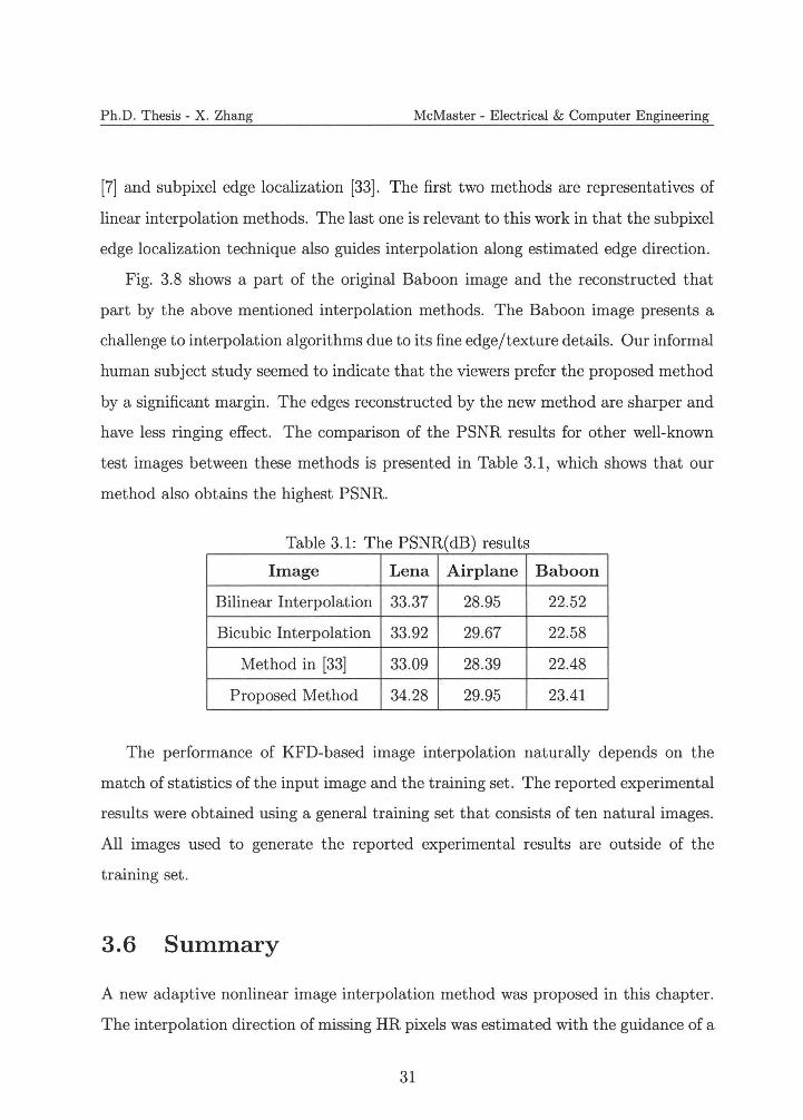
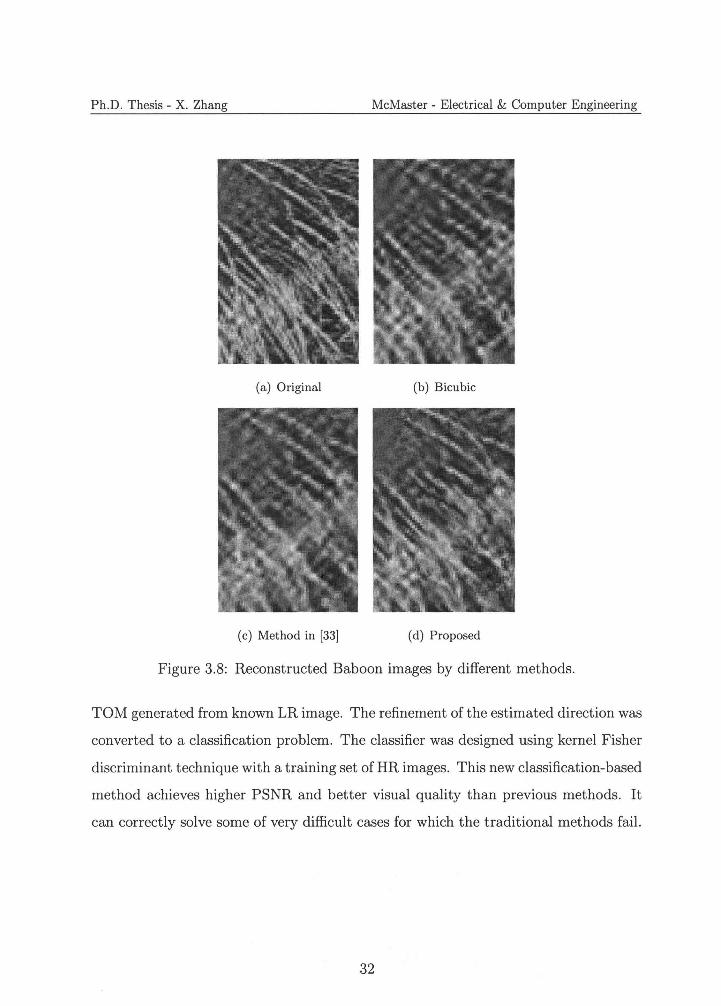
Fig. 3.8 shows a part of the original Baboon image and the reconstructed that
part by the above mentioned interpolation methods. The Baboon image presents a
challenge to interpolation algorithms due to its fine edge/texture details. Our informal
human subject study seemed to indicate that the viewers prefer the proposed method
by a significant margin. The edges reconstructed by the new method are sharper and
have less ringing effect . The comparison of the PSNR results for other well-known
test images between these methods is presented in Table 3.1, which shows that our
method also obtains the highest PSNR.
Table 3.1: The PSNR(dB) results
Image Lena Airplane Baboon
Bilinear Interpolation 33.37 28.95 22.52
Bicubic Interpolation 33.92 29.67 22.58
Method in [33] 33.09 28.39 22.48
Proposed Method 34.28 29.95 23.41
The performance of KFD-based image interpolation naturally depends on the
match of statistics of the input image and the training set. The reported experimental
results were obtained using a general training set that consists of ten natural images.
All images used to generate the reported experimental results are outside of the
training set .
3.6 Summary
A new adaptive nonlinear image interpolation method was proposed in this chapter.
The interpolation direction of missing HR pixels was estimated with the guidance of a
31
Ph.D. Thesis - X. Zhang McMaster - Electrical & Computer Engineering
(a) Original (b) Bicubic
(c) Method in [33] ( d) Proposed
Figure 3.8: Reconstructed Baboon images by different methods.
TOM generated from known LR image. The refinement of the estimated direction was
converted to a classification problem. The classifier was designed using kernel Fisher
discriminant technique with a training set of HR images. This new classification-based
method achieves higher PSNR and better visual quality than previous methods. It
can correctly solve some of very difficult cases for which the traditional methods fail.
32
Ph.D. Thesis - X. Zhang McMaster - Electrical & Computer Engineering
Chapter 4
Soft-decision Adaptive
Interpolation
In previous chapter, we described an adaptive nonlinear interpolation method that
assumes and uses some prior knowledge learnt from a training set of HR images. But
the performance of the learning approach degrades if there is a statistical mismatch
between the input image and the training set. Unless the input images are confined
to a narrow known class (e.g., faces), it is prudent to estimate the HR image using
primarily the statistics available in the input LR image. In this and subsequent
chapters we develop adaptive image interpolation methods without the use of training
HR images. Instead we boost the performance of these methods by introducing a
class of versatile parametric image models: 2D piecewise autoregressive process. The
model parameters are estimated in a moving window in the input LR image. The
pixel structure dictated by the learnt model is enforced by a soft-decision estimation
process onto a block of pixels, including both observed and estimated.
33
Ph.D. Thesis - X. Zhang McMaster - Electrical & Computer Engineering
4.1 Overview
The reproduction quality of any image interpolation algorithm primarily depends on
its adaptability to varying pixel structures across an image. In fact , modeling of non
stationarity of image signals is a common challenge facing many image processing
tasks, such as compression, restoration, denoising, and enhancement. Wu et al. [72]
had a measured success in this regard in a research on predictive lossless image com
pression. In that work a natural image is modeled as a piecewise 2D autoregressive
process. The model parameters are estimated on the fly for each pixel using sample
statistics of a local window, assuming that the image is piecewise stationary. In this
work we extend this approach to image interpolation. An obvious difference is in
that the sample set for parameter estimation has to be causal to the current pixel
for predictive coding, but does not need to be so for interpolation, which is to the
advantage of the latter task. On the other hand, for image interpolation the fit of
the model to the true high-resolution image signal is made more difficult by the fact
that only a low-resolution version of the original can be observed.
All image interpolation methods involve fitting missing pixels to some sample
structure learnt from the low resolution image. This is best accomplished by esti
mating a block of missing pixels in relation to the nearby known pixels rather than
estimating the individual missing pixels in isolation as done in the literature up to
now. The main result of this chapter is a new image interpolation technique, called
soft-decision adaptive interpolation (SAI) . The SAI technique, via a natural inte
gration of piecewise two-dimensional autoregressive modeling and block estimation,
achieves superior image interpolation results to those reported in the literature. It is
shown that the new SAI technique is equivalent to interpolation using an adaptive
non-separable 2D filter of high order.
The rest of the chapter is structured as follows. Section 4.2 defines a two
dimensional piecewise autoregressive (PAR) image model to facilitate the subsequent
development. Section 4.3 presents the most important result of this work: a soft
34
Ph.D. Thesis - X. Zhang McMaster - Electrical & Computer Engineering
decision estimation technique for adaptive image interpolation. Section 4.4 discusses
how to estimate the PAR model parameters in the low-resolution image. Implemen
tation details of the SAi algorithm are presented in Section 4.5, where the reader can
also gain an insight into the inner work of the SAi technique. Experimental results
and a comparison study with some existing popular image interpolation techniques
are presented in Section 4.6. Section 4. 7 concludes.
4.2 Piecewise Stationary Autoregressive Model
For the purpose of adaptive image interpolation, we model the image as a piecewise
autoregressive process:
X(i,j) = L au,vX(i - u,j - v) + Vi,j ( 4.1) (u,v)ET
where T is a spatial template for the regression operation. The term vi,j is a random
perturbation independent of spatial location ( i, j) and the image signal, and it ac
counts for both fractal-like fine details of image signal and measurement noise. The
validity of the PAR model hinges on a mechanism that adjusts the model parameters
au,v to local pixel structures. The fact that semantically meaningful image constructs,
such as edges and surface textures, are formed by spatially coherent contiguous pixels,
suggests piecewise statistical stationarity of the image signal. In other words, in the
setting of the PAR model, the parameters au,v remain constant or near constant in a
small locality, although they may and often do vary significantly in different segments
of a scene. The piecewise stationarity makes it possible to learn pixel structures such
as edges and textures by fitting samples of a local window to the PAR model.
The validity of the PAR model with locally adaptive parameters is corroborated
by the success of this modeling technique in lossless image compression. Among
all known lossless image coding methods, including CALIC (context-based adaptive
lossless codec) [1], TMW [4], and invertible integer wavelets [73], those that employ
35
Ph.D. Thesis - X. Zhang McMaster - Electrical & Computer Engineering
the PAR model with adjusted parameters on a pixel-by-pixel basis have delivered
the lowest lossless bit rates [72, 74] . In the principle of Kolmogorov complexity, the
true model of a stochastic process is the one that yields the minimum description
length. Thus we have strong empirical evidence to support the appropriateness and
usefulness of the PAR model for natural images.
In the next section, we will integrate the PAR model into a soft-decision estimation
framework for the purpose of image interpolation, and develop the SAI algorithm.
4.3 Adaptive Interpolation with Soft Decision
First we introduce some notations that are necessary for the description of the SAI
algorithm. Let h be the HR image to be estimated by interpolating the observed
LR image h Same as in the previous chapter, the LR image 11 is a down sampled
version of the HR image h by a factor of two. Let Yi E 11 and Xi E h be the pixels
of images 11 and h respectively. We write the neighbors of pixel location i in the HR
image as Xiot, t = 1, 2, · · ·. Since Yi E 11 implies Yi E h, we also write an HR pixel
xi E h as Yi (likewise, Xiot as Yiot) when it is in the LR image, xi E /z, as well.
The SAI algorithm interpolates the missing pixels in h in two passes in a coarse
to fine progression. The work of the two passes is shown by Fig. 4.1, in which
the solid dots are known LR pixels, the shaded dots are those missing pixels to be
interpolated in the first pass, and the empty dots are the remaining missing pixels
to be interpolated in the second pass. The pixels generated by the first pass and
the known LR pixels form a quincunx sublattice of the HR image (the union of solid
and shaded dots) . The second pass completes the reconstruction of the HR image by
interpolating the other quincunx sublattice of empty dots.
Fig. 4.2(a) illustrates the spatial configuration of known and missing pixels in
volved in the first pass. To avoid intricate notations, from now on we use a single
position index to denote a pixel location instead of two dimensional coordinates. For
36
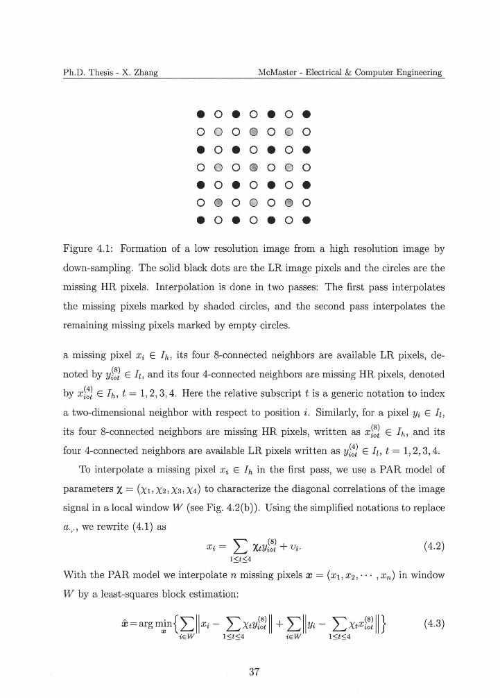
Ph.D. Thesis - X. Zhang McMaster - Electrical & Computer Engineering
• 0 • 0 • 0 • 0 0 0 0 0 0 0
• 0 • 0 • 0 • 0 0 0 0 0 0 0
• 0 • 0 • 0 • 0 0 0 0 0 0 0
• 0 • 0 • 0 • Figure 4.1: Formation of a low resolution image from a high resolution image by
down-sampling. The solid black dots are the LR image pixels and the circles are the
missing HR pixels. Interpolation is done in two passes: The first pass interpolates
the missing pixels marked by shaded circles, and the second pass interpolates the
remaining missing pixels marked by empty circles.
a missing pixel Xi E h, its four 8-connected neighbors are available LR pixels, de
noted by y~£ E 11, and its four 4-connected neighbors are missing HR pixels, denoted
by x~!i E h, t = 1, 2, 3, 4. Here the relative subscript t is a generic notation to index
a two-dimensional neighbor with respect to position i. Similarly, for a pixel Yi E 11,
its four 8-connected neighbors are missing HR pixels, written as x~!i E h, and its
four 4-connected neighbors are available LR pixels written as y}!£ E Ii, t = 1, 2, 3, 4.
To interpolate a missing pixel Xi E h in the first pass, we use a PAR model of
parameters X = (x1 , x2 , x3 , x4 ) to characterize the diagonal correlations of the image
signal in a local window W (see Fig. 4.2(b)). Using the simplified notations to replace
a. ,., we rewrite (4.1) as
- ~ (8)Xi - ~ XtYiot +'Vi· (4.2)
19'.'::4
With the PAR model we interpolate n missing pixels x = (x1 , x2 , · · · , xn) in window
W by a least-squares block estimation:
37
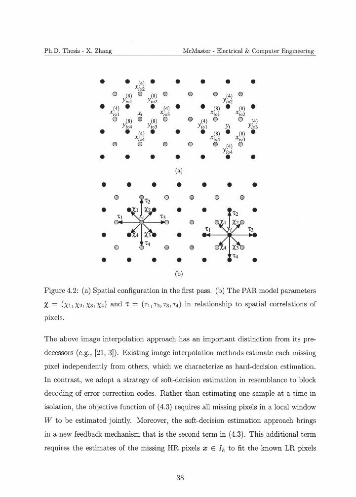
• • • • • • • • • • • • • •
• • • • • • •
• • • • • • •
• • • • • • •
• •
• • • •
Ph.D. Thesis - X. Zhang McMaster - Electrical & Computer Engineering
• 't4 •
(4) xio2
0 0 0 0 0 0(8) (8) (4) Yiol Yio2 Y;o2
(4) (4) (8) (8) xi<>I Xj xi<>3 xi<> I xi<>2 0 0 0 0 0 0(8) (8) (4) (4)
Yi<>4 Y;o3 Yiol Yi Y;o3 (4) (8) (8)
xi<>4 X;<>4 xi<>3 0 0 0 0 0 0(4)
Y;<>4
(a)
0 0 0 0 0
0
• • 0
(b)
Figure 4.2: (a) Spatial configuration in the first pass. (b) The PAR model parameters
X = (x1, X2, X3 , X4) and 't = (T1 ,T2 , T3,T4) in relationship to spatial correlations of
pixels.
The above image interpolation approach has an important distinction from its pre
decessors (e.g., [21 , 3]). Existing image interpolation methods estimate each missing
pixel independently from others, which we characterize as hard-decision estimation.
In contrast, we adopt a strategy of soft-decision estimation in resemblance to block
decoding of error correction codes. Rather than estimating one sample at a time in
isolation, the objective function of ( 4.3) requires all missing pixels in a local window
W to be estimated jointly. Moreover, the soft-decision estimation approach brings
in a new feedback mechanism that is the second term in (4.3) . This additional term
requires the estimates of the missing HR pixels x E h to fit the known LR pixels
38
Ph.D. Thesis - X. Zhang McMaster - Electrical & Computer Engineering
y E 11 with the very same PAR model that fits y E 11 to x E h. Aided by the
feedback mechanism that accounts for mutual influences between the estimates of
the missing pixels in a local window W, the SAi algorithm can mitigate errors of
hard-decision estimation by preventing the PAR model, when applied to estimated
HR pixels x Eh, from being violated on neighboring known LR pixels y E ]z.
To include horizontal and vertical correlations into the SAi algorithm, we intro
duce four more parameters 't = (T1, T2 , T3 , T4 ) whose geometric meanings are shown in
Fig. 4.2(b) . These parameters 'tare used to impose the same directional correlation
between LR pixels Yi and y~f on between HR pixels Xi and x~!i, namely
Xi= L llTtX~;; II+ Vi · (4.4) 19:-::;4
The soft-decision estimation technique can incorporate (4.4) into (4.3) . But one
should practise caution since the pixels Xi and x~!l in ( 4.4) are all unknown. By using
a Lagrangian multiplier A to regulate the contribution of (4.4), we extend (4.3) to the
following constrained optimal block estimation problem:
l(A) = m~n{I:llxi - L XtY~ill iEW 199
+ I:llYi - L XtX~!lll +A I:llxi - L Ttx~!lll}iEW 1:-=;t9 iEW 199 (4.5)
subject to
In minimizing l(A) the value of A is chosen such that .l:::w llxi - 2::::1:-::;t:-:;4 Ttx~;i II ~ .l:::w II Yi - 2::::199 TtY~i II· The SAi algorithm iterates on A until the constraint is
satisfactorily met, by decreasing A if the left side of the constraint is less than the
right side and vise versa. This constraint holds if the sample statistics is shift invariant
in the window W. We observe that the value of A is in the range of 0.2 rv 0.7 when
meeting the constraint. For most natural images, one can simply choose A = 0.5 with
no material loss of performance compared with the iteratively computed A.
39
Ph.D. Thesis - X. Zhang McMaster - Electrical & Computer Engineering
Compared to existing autoregressive methods that use parameters X only [3, 42],
the SAI algorithm expands the model parameter space by using two sets of parame
ters 't and X· The expanded PAR model has the potential of representing the high
resolution image more accurately than in [3, 42]. However, to circumvent the risk
of data overfitting, we do not directly use an autoregressive model of order 8, but
rather split model parameters X and 'tin two separate terms of the objective function
(4.5). In fact, in separation from x, the parameters 't can be better estimated than
parameters X using samples in the LR image, as we will see in the next section.
With the block-based soft-decision estimation and the increased order in piecewise
autoregressive modeling, the new SAI algorithm achieves unprecedented interpolation
accuracy. More importantly it performs consistently well over a wide range of images,
and the performance is far less sensitive to feature scales than existing techniques. We
will return to these points in Section 4.6 when the experimental results are presented
and discussed.
Up to now we have only described the interpolation process of the first pass. Once
the missing HR pixels in the first pass are interpolated as described above, half of
the HR pixels are obtained. The remaining half of the missing HR pixels are to be
interpolated in the second pass. The interpolation problem in the second pass is
essentially the same as in the first pass. The only difference is that the SAI algorithm
now interpolates the missing HR pixels xi E h using their four 4-connected neighbors,
which are either known in 11 or estimated in the first pass. The problem has the same
formulation as in (4.5), if we simply rotate the spatial configuration of Fig. 4.2(a) by
45 degrees (see Fig. 4.3).
4.4 Model Parameter Estimation
A key to the success of the SAI algorithm is how well the model parameters X and 't
in ( 4.5) can be estimated using LR image samples. Referring to the spatial relation
40
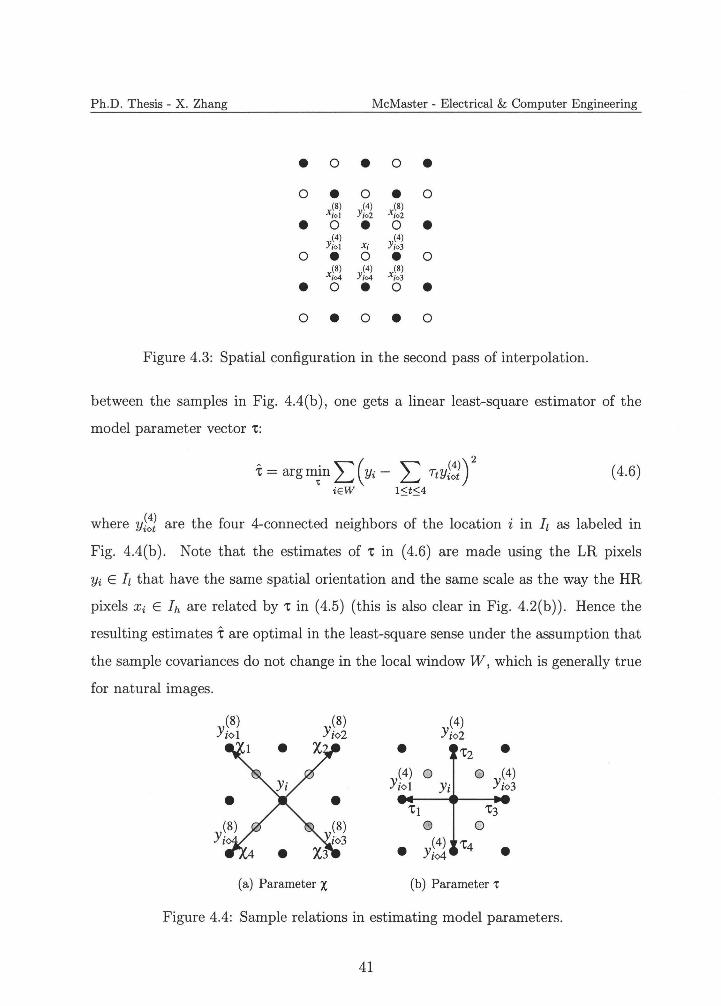
• • • • •
• • • • •
• • • • •
Ph.D. Thesis - X. Zhang McMaster - Electrical & Computer Engineering
0 0
0 0 0 (8) (4) (8)
Xio l Y;oz Xio2
0 0 (4) (4)
Y;o1 x; Y;o3
0 0 0 (8) (4) (8)
X;o4 Y;o4 X;o3
0 0
0 0 0
Figure 4.3: Spatial configuration in the second pass of interpolation.
between the samples in Fig. 4.4(b), one gets a linear least-square estimator of the
model parameter vector 't:
i = argmJn L(Yi - L TtY~lr (4.6) iEW l::;t:S:4
where y;;; are the four 4-connected neighbors of the location i in 11 as labeled in
Fig. 4.4(b) . Note that the estimates of 't in (4.6) are made using the LR pixels
Yi E 11 that have the same spatial orientation and the same scale as the way the HR
pixels xi E h are related by 'tin (4.5) (this is also clear in Fig. 4.2(b)). Hence the
resulting estimates i are optimal in the least-square sense under the assumption that
the sample covariances do not change in the local window W, which is generally true
for natural images.
(8) (4) Yiol Yio2
't2• • (4) 0 0 (4)
Yio3 Yiol Yi
't1 0
• (4) 't4 •Yio4
(a) Parameter X (b) Parameter 't
Figure 4.4: Sample relations in estimating model parameters.
41
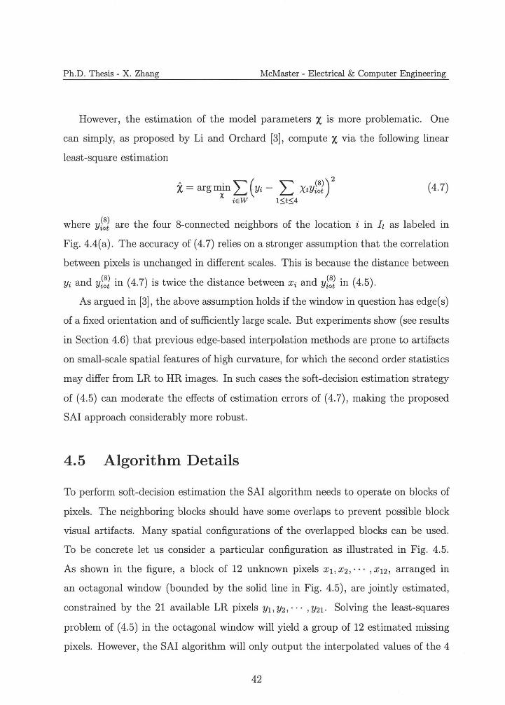
Ph.D. Thesis - X. Zhang McMaster - Electrical & Computer Engineering
However, the estimation of the model parameters X is more problematic. One
can simply, as proposed by Li and Orchard [3], compute X via the following linear
least-square estimation
A - o (8)X - argmm L ( Yi - L XtYiot )
2 (4.7)
X iEW 19::04
where y~l are the four 8-connected neighbors of the location i in !1 as labeled in
Fig. 4.4(a) . The accuracy of (4.7) relies on a stronger assumption that the correlation
between pixels is unchanged in different scales. This is because the distance between
Yi and Yi~l in (4.7) is twice the distance between xi and Yi~l in (4.5).
As argued in [3], the above assumption holds if the window in question has edge(s)
of a fixed orientation and of sufficiently large scale. But experiments show (see results
in Section 4.6) that previous edge-based interpolation methods are prone to artifacts
on small-scale spatial features of high curvature, for which the second order statistics
may differ from LR to HR images. In such cases the soft-decision estimation strategy
of (4.5) can moderate the effects of estimation errors of (4.7), making the proposed
SAi approach considerably more robust.
4.5 Algorithm Details
To perform soft-decision estimation the SAi algorithm needs to operate on blocks of
pixels. The neighboring blocks should have some overlaps to prevent possible block
visual artifacts. Many spatial configurations of the overlapped blocks can be used.
To be concrete let us consider a particular configuration as illustrated in Fig. 4.5.
As shown in the figure, a block of 12 unknown pixels x1, x2 , · · · , x12 , arranged in
an octagonal window (bounded by the solid line in Fig. 4.5), are jointly estimated,
constrained by the 21 available LR pixels y1 , y2 , • • · , y21 . Solving the least-squares
problem of ( 4.5) in the octagonal window will yield a group of 12 estimated missing
pixels. However, the SAi algorithm will only output the interpolated values of the 4
42
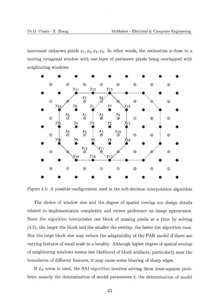
• • • • • • • • •
• • •
• • •
• • • • • • • • •
Ph.D. Thesis - X. Zhang McMaster - Electrical & Computer Engineering
innermost unknown pixels x1 , x2 , x3 , X4 . In other words, the estimation is done in a
moving octagonal window with one layer of perimeter pixels being overlapped with
neighboring windows.
0 0 0 0 0 0 0 0 Yll Y12 YB
-------~------• • , .. • •' ' X7 Xg/ 0 0 0
• ,
Y6 YL' Y7
I IXI x2 X9I
0 I0 I
0 0
• Y4 n Y2
X4 X3 XIo 0 0 0 0
• y Y9 Y6 Ys•,
I
',~11• XI2 •
0
• 0 G,
• ',YI
' ' 0 0 0 '•
' '
'• • 0 0 0
• I
• I I
•I I
, , • I
• 0 0
I 0
• ,
I I
0 ,0 0 , ,
,
• •---------------· 0 0 0 0 0 0 0 0
Figure 4.5: A possible configuration used in the soft-decision interpolation algorithm
The choice of window size and the degree of spatial overlap are design details
related to implementation complexity and viewer preference on image appearance.
Since the algorithm interpolates one block of missing pixels at a time by solving
(4.5) , the larger the block and the smaller the overlap, the faster the algorithm runs.
But the large block size may reduce the adaptability of the PAR model if there are
varying features of small scale in a locality. Although higher degree of spatial overlap
of neighboring windows means less likelihood of block artifacts, particularly near the
boundaries of different features , it may cause some blurring of sharp edges.
If £ 2 norm is used, the SAI algorithm involves solving three least-squares prob
lems, namely the determination of model parameters 't, the determination of model
43
Ph.D. Thesis - X. Zhang McMaster - Electrical & Computer Engineering
parameters x, and the minimization problem of (4.5). For each block we can compute
't and X in the closed form solutions of (4.6) and (4.7). Namely,
(4.8)
where the column vector b is composed of all LR pixels Yi inside the block. The ith
row of matrix B consists of the four 4-connected neighbors y~£ of Yi, t = 1, 2, 3, 4.
And,
(4.9)
where the ith row of matrix A consists of the four 8-connected neighbors y~£ of Yi,
t = 1, 2,3,4.
We rewrite (4.5) in matrix form:
(4.10)
where x = (x1, x2 , • · · , x12 ) is the vector of the 12 unknown pixels in the current
octagon window as labeled in Fig. 4.5, y = (y1 , y2 , · • · , y21 ) is the vector of the 21
available LR pixels inside and on the boundary of the octagon window in Fig. 4.5,
and
(4.11)D=C=
where I is the identity matrix with the subscript being its dimension, 0 is the zero
matrix whose dimension is indicated by the subscript, >. is the Lagrangian factor in
(4.5) , and
44
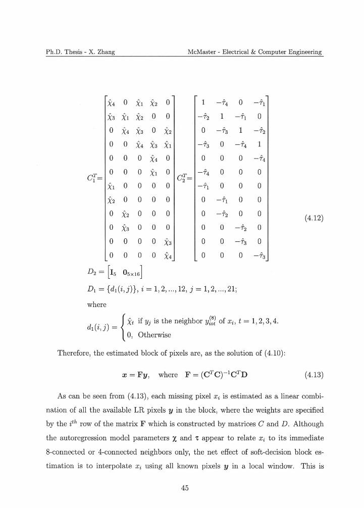
Ph.D. Thesis - X. Zhang McMaster - Electrical & Computer Engineering
1 -T4 0 -T1
X3 x1 x2 0 0
X4 0 x1 X2 0
-T2 1 -T1 0
0 X4 X3 0 X2 0 -T3 1 -f2
0 0 X4 X3 X1 -T3 0 -f4 1
0 0 0 X4 0 0 0 0 -T4
0 0 0 X1 0 -T4 0 0 0 Cf= Ci=
0 0 0 0 -f1 0 0 0X1
x2 0 0 0 0 0 -T1 0 0
0 x2 0 0 0 0 -T2 0 0 (4.12) 0 X3 0 0 0 0 0 -T2 0
0 0 0 0 X3 0 0 -T3 0
0 0 0 0 X4 0 0 0 -T3
D2 = [15 Os xl6]
D1 = {d1(i,j)}, i = 1, 2, ... , 12, j = 1, 2, .. . , 21;
where
{ x. if y1 is the neighbor y~l of xi, t = 1, 2, 3, 4. d1(i , J ) -
0, Otherwise
Therefore , the estimated block of pixels are , as the solution of (4.10):
(4.13)
As can be seen from ( 4.13) , each missing pixel xi is estimated as a linear combi
nation of all the available LR pixels y in the block, where the weights are specified
by the ith row of the matrix F which is constructed by matrices C and D . Although
the autoregression model parameters X and 't appear to relate xi to its immediate
8-connected or 4-connected neighbors only, the net effect of soft-decision block es
timation is to interpolate xi using all known pixels y in a local window. This is
45
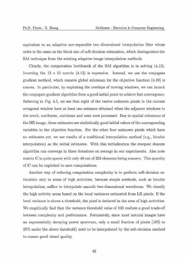
Ph.D. Thesis - X. Zhang McMaster - Electrical & Computer Engineering
equivalent to an adaptive non-separable two dimensional interpolation filter whose
order is the same as the block size of soft-decision estimation, which distinguishes the
SAi technique from the existing adaptive image interpolation methods.
Clearly, the computation bottleneck of the SAi algorithm is in solving (4.13).
Inverting the 12 x 12 matrix ( 4.13) is expensive. Instead, we use the conjugate
gradient method, which ensures global minimum for the objective function (4.10) is
convex. In particular, by exploiting the overlaps of moving windows, we can launch
the conjugate gradient algorithm from a good initial point to achieve fast convergence.
Referring to Fig. 4.5, we see that eight of the twelve unknown pixels in the current
octagonal window have at least one estimate obtained when the adjacent windows to
the north, northwest, northeast and west were processed. Due to spatial coherence of
the HR image, these estimates are statistically good initial values of the corresponding
variables in the objective function. For the other four unknown pixels which have
no estimates yet, we use results of a traditional interpolation method (e.g., bicubic
interpolation) as the initial estimates. With this initialization the steepest descent
algorithm can converge in three iterations on average in our experiments. Also note
matrix C is quite sparse with only 49 out of 252 elements being nonzero. This sparsity
of C can be exploited to save computations.
Another way of reducing computation complexity is to perform soft-decision es
timation only in areas of high activities, because simple methods, such as bicubic
interpolation, suffice to interpolate smooth two-dimensional waveforms. We classify
the high activity areas based on the local variances estimated from LR pixels. If the
local variance is above a threshold, the pixel is declared in the area of high activities.
We empirically find that the variance threshold value of 100 realizes a good trade-off
between complexity and performance. Fortunately, since most natural images have
an exponentially decaying power spectrum, only a small fraction of pixels (10% to
25% under the above threshold) need to be interpolated by the soft-decision method
to ensure good visual quality.
46
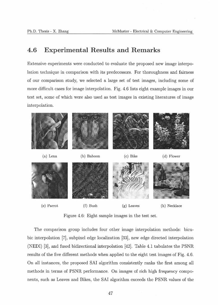
Ph.D. Thesis - X. Zhang McMaster - Electrical & Computer Engineering
4.6 Experimental Results and Remarks
Extensive experiments were conducted to evaluate the proposed new image interpo
lation technique in comparison with its predecessors. For thoroughness and fairness
of our comparison study, we selected a large set of test images, including some of
more difficult cases for image interpolation. Fig. 4.6 lists eight example images in our
test set, some of which were also used as test images in existing literatures of image
interpolation.
(a) Lena (b) Baboon (c) Bike (d) Flower
(e) Parrot (f) Bush (g) Leaves (h) Necklace
Figure 4.6: Eight sample images in the test set.
The comparison group includes four other image interpolation methods: bicu
bic interpolation [7], subpixel edge localization [33], new edge directed interpolation
(NEDI) [3], and fused bidirectional interpolation [42] . Table 4.1 tabulates the PSNR
results of the five different methods when applied to the eight test images of Fig. 4.6.
On all instances, the proposed SAI algorithm consistently ranks the first among all
methods in terms of PSNR performance. On images of rich high frequency compo
nents, such as Leaves and Bikes, the SAI algorithm exceeds the PSNR values of the
47
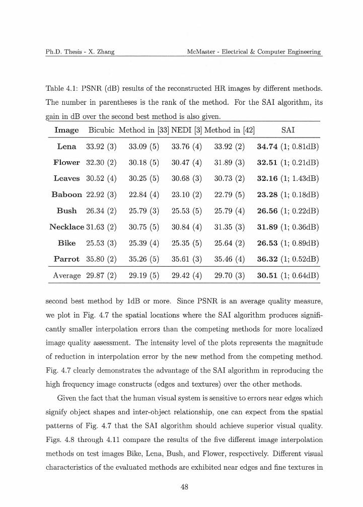
Ph.D. Thesis - X. Zhang McMaster - Electrical & Computer Engineering
Table 4.1: PSNR (dB) results of the reconstructed HR images by different methods.
The number in parentheses is the rank of the method. For the SAi algorithm, its
gain in dB over the second best method is also given.
Image Bicubic Method in [33] NEDI [3] Method in [42] SAI
Lena 33.92 (3) 33.09 (5) 33.76 (4) 33.92 (2) 34.74 (1; 0.8ldB)
Flower 32.30 (2) 30.18 (5) 30.47 ( 4) 31.89 (3) 32.51 (1; 0.2ldB)
Leaves 30.52 (4) 30.25 (5) 30.68 (3) 30.73 (2) 32.16 (1; l.43dB)
Baboon 22.92 (3) 22.84 (4) 23.10 (2) 22.79 (5) 23.28 (1; 0.18dB)
Bush 26.34 (2) 25.79 (3) 25.53 (5) 25 .79 (4) 26.56 (1; 0.22dB)
Necklace 31.63 (2) 30.75 (5) 30.84 (4) 31.35 (3) 31.89 (1; 0.36dB)
Bike 25.53 (3) 25.39 (4) 25.35 (5) 25.64 (2) 26.53 (1; 0.89dB)
Parrot 35.80 (2) 35.26 (5) 35.61 (3) 35.46 (4) 36.32 (1; 0.52dB)
Average 29.87 (2) 29.19 (5) 29.42 (4) 29.70 (3) 30.51 (1; 0.64dB)
second best method by ldB or more. Since PSNR is an average quality measure,
we plot in Fig. 4.7 the spatial locations where the SAi algorithm produces signifi
cantly smaller interpolation errors than the competing methods for more localized
image quality assessment. The intensity level of the plots represents the magnitude
of reduction in interpolation error by the new method from the competing method.
Fig. 4.7 clearly demonstrates the advantage of the SAi algorithm in reproducing the
high frequency image constructs (edges and textures) over the other methods.
Given the fact that the human visual system is sensitive to errors near edges which
signify object shapes and inter-object relationship, one can expect from the spatial
patterns of Fig. 4.7 that the SAi algorithm should achieve superior visual quality.
Figs. 4.8 through 4.11 compare the results of the five different image interpolation
methods on test images Bike, Lena, Bush, and Flower, respectively. Different visual
characteristics of the evaluated methods are exhibited near edges and fine textures in
48
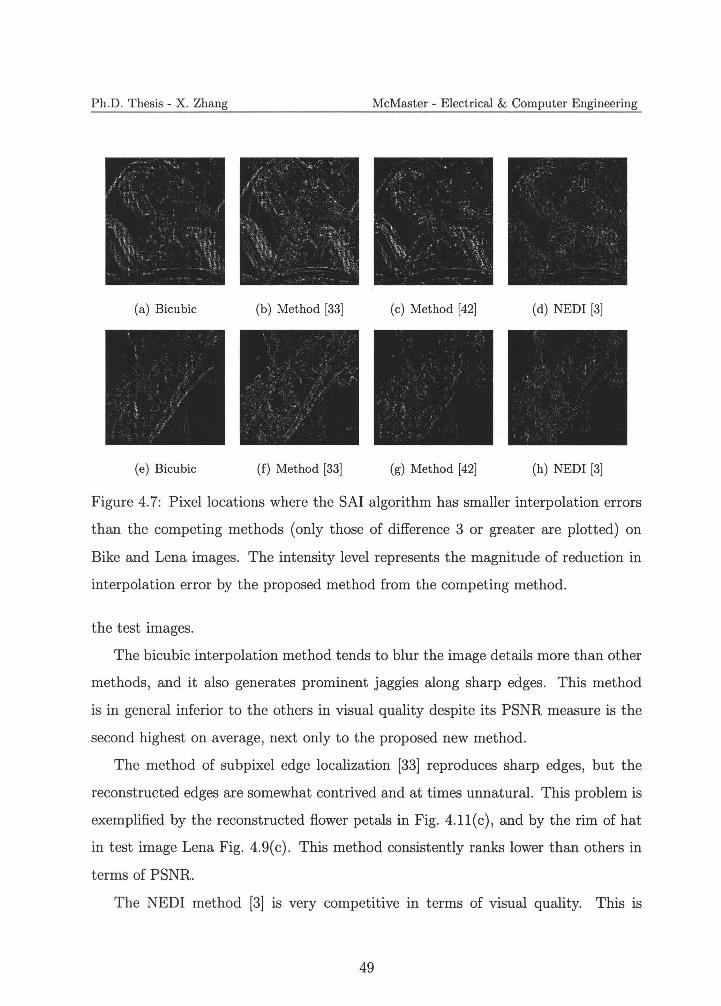
Ph.D. Thesis - X. Zhang McMaster - Electrical & Computer Engineering
(a) Bicubic (b) Method [33] (c) Method [42] (d) NEDI [3]
(e) Bicubic (f) Method [33] (g) Method [42] (h) NEDI [3]
Figure 4.7: Pixel locations where the SAI algorithm has smaller interpolation errors
than the competing methods (only those of difference 3 or greater are plotted) on
Bike and Lena images. The intensity level represents the magnitude of reduction in
interpolation error by the proposed method from the competing method.
the test images.
The bicubic interpolation method tends to blur the image details more than other
methods, and it also generates prominent jaggies along sharp edges. This method
is in general inferior to the others in visual quality despite its PSNR measure is the
second highest on average, next only to the proposed new method.
The method of subpixel edge localization [33] reproduces sharp edges, but the
reconstructed edges are somewhat contrived and at times unnatural. This problem is
exemplified by the reconstructed flower petals in Fig. 4.ll(c), and by the rim of hat
in test image Lena Fig. 4.9( c). This method consistently ranks lower than others in
terms of PSNR.
The NEDI method [3] is very competitive in terms of visual quality. This is
49
Ph.D. Thesis - X. Zhang McMaster - Electrical & Computer Engineering
primarily because it preserves long edges well. But in high activity areas where
features have small curvatures or multiple edges intersect, this method sometimes
generates speckle interpolation noises and ringing artifacts, as shown in Fig. 4.8( e)
and Fig. 4.ll(e), and more clearly in close-up parts of the reconstructed images in
Fig. 4.12. Such flaws are the reason that this method only ranks the forth in PSNR
in the comparison group of five methods, although it achieves pleasant visual effects
on large edge structures.
The fused bidirectional interpolation method [42] takes a middle ground between
the direction-less bicubic interpolation and edge-directed interpolation. It reproduces
sharper large scale edges than the bicubic method, but the reconstruction is not as
good as the method of [3] when the LR image contains enough information to correctly
learn the edge direction. However, on small scale features where the edge direction
learnt from the LR image is not reliable, this method can reduce speckle interpolation
noises via the MMSE fusion process. It is interesting to note that the fusion method
ranks in between the bicubic method and the method of [3] in PSNR.
As being evident in Figs. 4.8 through 4.11, the SAi algorithm eliminates most of
the visual defects associated with the other methods. It reproduces visually more
pleasant HR images than NEDI method that is considered as one of the best so far.
Please refer to Fig. 4.12 for a side-by-side comparison between the two methods. Of
particular significance is the fact that the SAi algorithm obtains superior visual qual
ity on image features of large and small scales alike. This robustness is attributed to
the soft-decision estimation technique that enforces the spatial coherence of estimated
pixels according to the PAR model.
Although the proposed SAi algorithm is presented to double the horizontal and
vertical resolutions, it can be readily generalized to scaling factor a = 2z with z being
a positive integer. One can simply apply the proposed SAi algorithm z times to scale
the input image by a times. For an arbitrary scaling factor a (not an integer power
of two), the interpolation can be done by first using the SAi algorithm to expand the
50
Ph.D. Thesis - X. Zhang McMaster - Electrical & Computer Engineering
input image by 2z times such that 2z < a < 2z+1, and then applying a conventional
image interpolation algorithm, such as bicubic or bilinear interpolation, to scale up
the output image of the new method bys times such that 2zs =a. Fig. 4.13 is an
example for scaling factor of 3, and it shows that the image interpolated by the SAi
algorithm followed by bicubic interpolation has better visual quality than the image
by bicubic interpolation only.
As described in section 4.4, the estimation of model parameters assumes that the
spatial correlation between the HR pixels is approximately the same as between LR
pixels. When this assumption is violated, the SAi algorithm may introduce some false
edges or textures due to over-fitting of LR data. This over-fitting problem can be seen
in Fig. 4.14. For this particular test image the spatial correlation changes after down
sampling, which causes the SAi algorithm to produce erroneous textures. There is
a way to detect where the over-fitting problem will likely occur. If the value of the
cost function ( 4.5) at the convergence of the SAi algorithm is above a threshold, then
chances are that the PAR model is not valid in the locality. As a recourse one can
switch to a more conservative method such as bicubic interpolation to prevent the
generation of false pixel structures. But this also tends to blur some sharp edges.
4.7 Conclusion
A novel soft-decision approach is proposed for adaptive image interpolation. When
coupled with a PAR image model, the soft-decision approach estimates a block of
missing pixels jointly by imposing an adaptively learnt spatial sample relation not only
between known pixels and missing pixels but also between missing pixels themselves.
This new image interpolation technique outperforms the existing methods in both
PSNR measure and subjective visual quality over a wide range of scenes, by preserving
the spacial coherence of the reconstructed high-resolution image on features of large
and small scales alike.
51
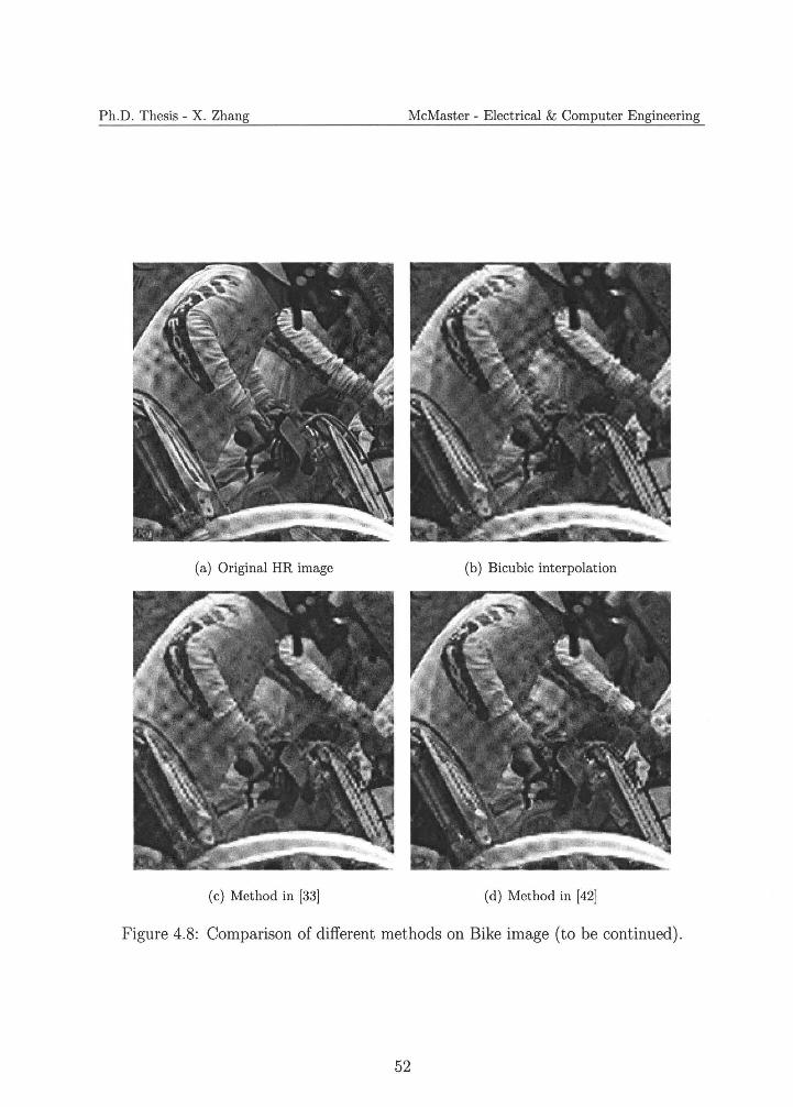
Ph.D. Thesis - X. Zhang McMaster - Electrical & Computer Engineering
(a) Original HR image (b) Bi cubic interpolation
(c) Method in [33] (d) Method in [42]
Figure 4.8: Comparison of different methods on Bike image (to be continued).
52
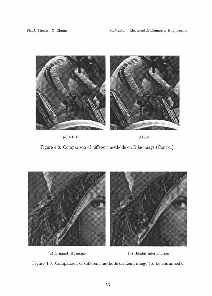
Ph.D. Thesis - X. Zhang McMaster - Electrical & Computer Engineering
(e) NEDI (f) SAI
Figure 4.8: Comparison of different methods on Bike image (Cont'd.).
(a) Original HR image (b) Bi cubic interpolation
Figure 4.9: Comparison of different methods on Lena image (to be continued).
53
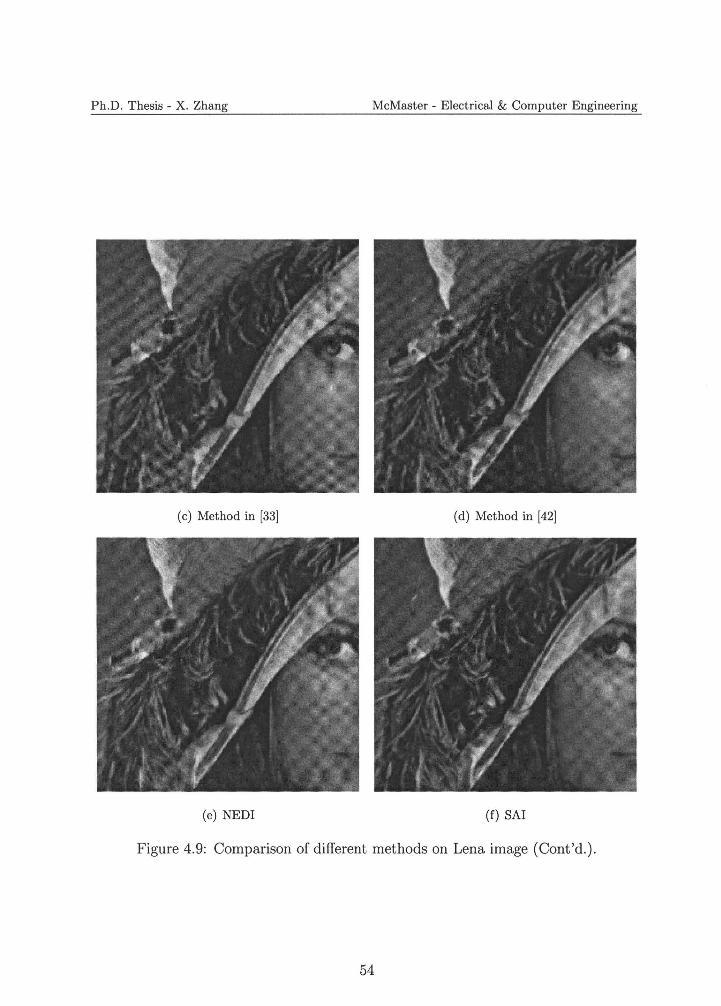
Ph.D. Thesis - X. Zhang McMaster - Electrical & Computer Engineering
(c) Method in [33] (d) Method in [42]
(e) NEDI (f) SAI
Figure 4.9: Comparison of different methods on Lena image (Cont'd.).
54
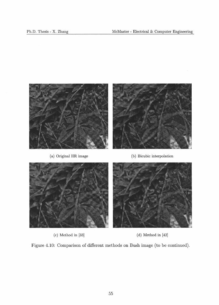
Ph.D. Thesis - X. Zhang McMaster - Electrical & Computer Engineering
(a) Original HR image (b) Bicubic interpolation
(c) Method in [33] (d) Method in [42]
Figure 4.10: Comparison of different methods on Bush image (to be continued) .
55
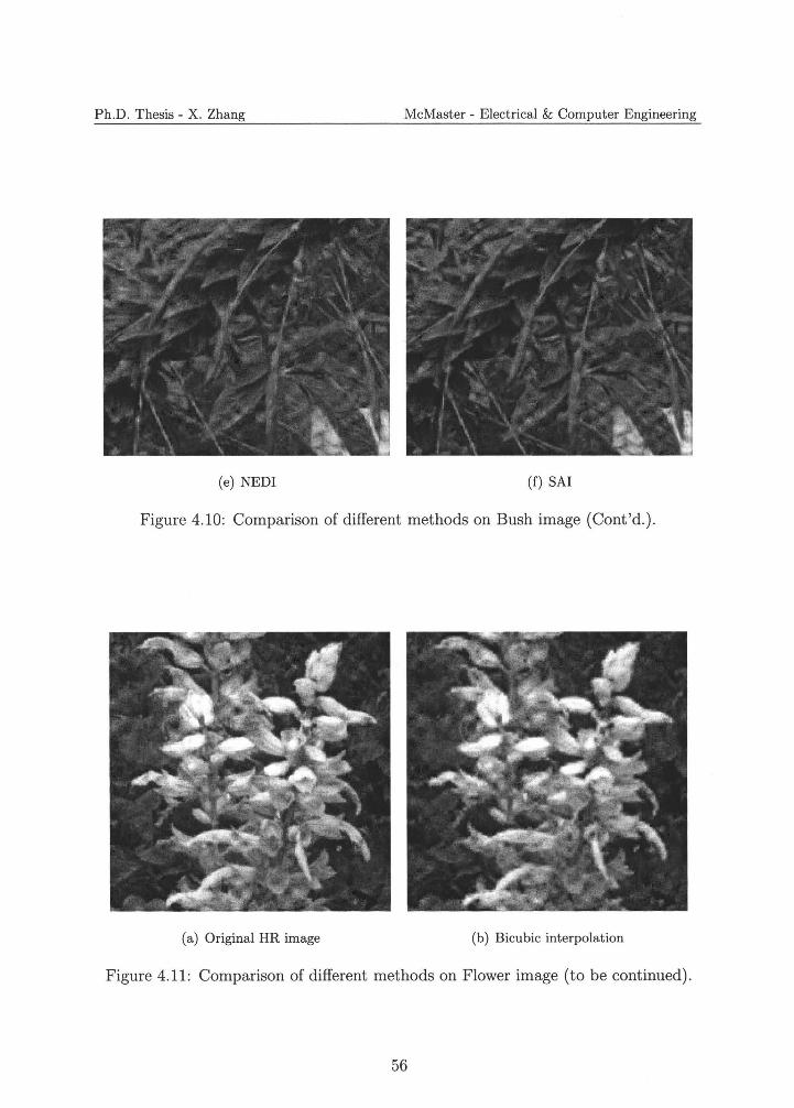
Ph.D. Thesis - X. Zhang McMaster - Electrical & Computer Engineering
(e) NEDI (f) SAi
Figure 4.10: Comparison of different methods on Bush image (Cont'd.).
(a) Original HR image (b) Bicubic interpolation
Figure 4.11: Comparison of different methods on Flower image (to be continued).
56
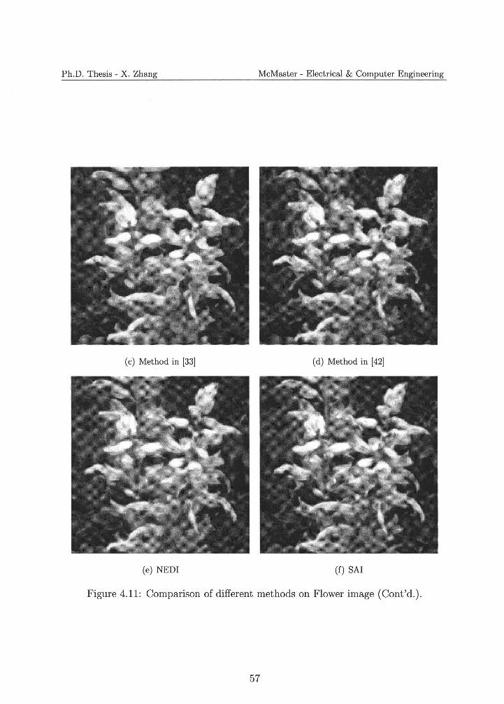
Ph.D. Thesis - X. Zhang McMaster - Electrical & Computer Engineering
(c) Method in [33] (d) Method in [42]
(e) NEDI (f) SAI
Figure 4.11 : Comparison of different methods on Flower image (Cont'd.).
57
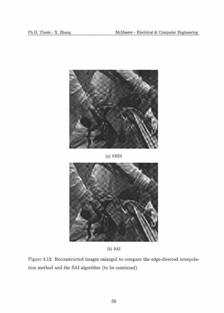
Ph.D. Thesis - X. Zhang McMaster - Electrical & Computer Engineering
(a) NEDI
(b) SAi
Figure 4.12: Reconstructed images enlarged to compare the edge-directed interpola
tion method and the SAi algorithm (to be continued).
58
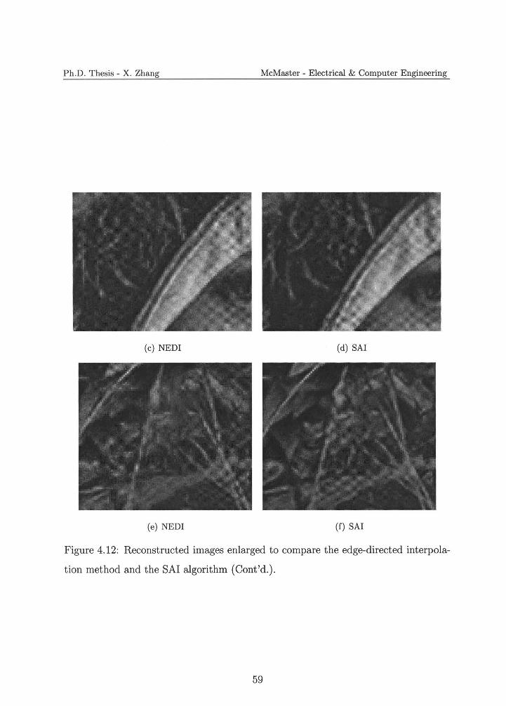
Ph.D. Thesis - X. Zhang McMaster - Electrical & Computer Engineering
(c) NEDI (d) SAI
(e) NEDI (f) SAI
Figure 4.12: Reconstructed images enlarged to compare the edge-directed interpola
tion method and the SAI algorithm (Cont'd.).
59
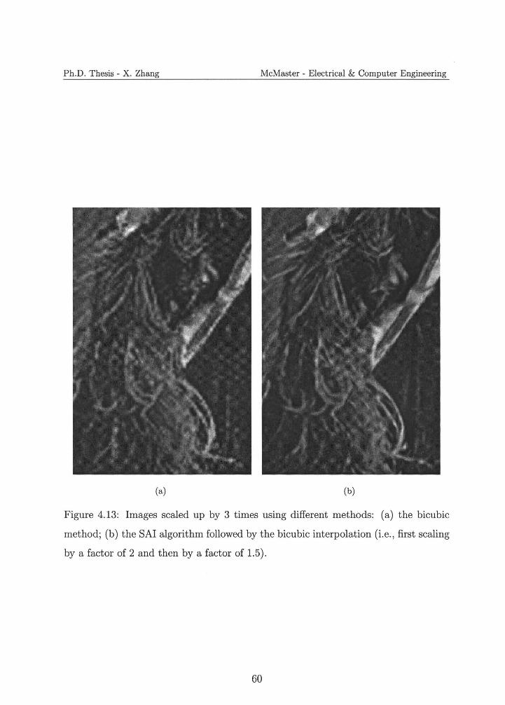
Ph.D. Thesis - X. Zhang McMaster - Electrical & Computer Engineering
(a) (b)
Figure 4.13: Images scaled up by 3 times using different methods: (a) the bicubic
method; (b) the SAI algorithm followed by the bicubic interpolation (i.e., first scaling
by a factor of 2 and then by a factor of 1.5) .
60
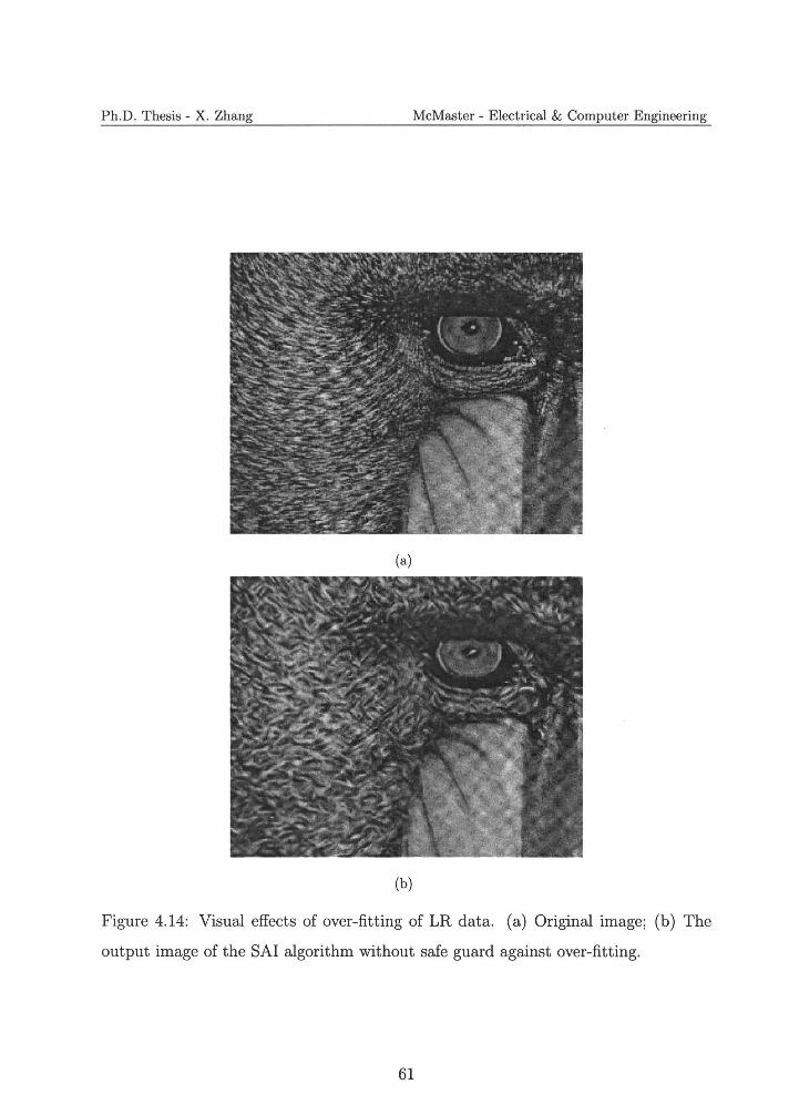
Ph.D. Thesis - X. Zhang McMaster - Electrical & Computer Engineering
(a)
(b)
Figure 4.14: Visual effects of over-fitting of LR data. (a) Original image; (b) The
output image of the SAi algorithm without safe guard against over-fitting.
61
Ph.D. Thesis - X. Zhang McMaster - Electrical & Computer Engineering
Chapter 5
Model-based Non-linear
Restoration
This chapter presents the most sophisticated image interpolation method developed
in this thesis research. This method improves its predecessors, including the previous
two methods, in two aspects. Firstly, a realistic model of LR image formation from
the corresponding HR image is integrated into the interpolation process. As such,
upsampling and deconvolution can be performed jointly rather than separately as
in existing methods, which improves interpolation performance by factoring in the
effect of the point spread function (PSF). Secondly, the new method can work with
an arbitrary scaling factor while the previous methods are restricted to scaling factors
that are power of two.
5 .1 Overview
As discussed in the previous chapter, the adaptability of the SAI algorithm comes
from a 2D PAR image model that can adapt to varying two-dimensional image signal
waveform. However, the SAI algorithm still suffers from a serious deficiency of mod
eling like its predecessors [3, 41]: the image model is learnt from the LR image but
62
Ph.D. Thesis - X. Zhang McMaster - Electrical & Computer Engineering
applied to reconstruct the HR image. The issue here is one of chicken and egg. On
one hand, correct interpolation of missing pixels relies on a good model of HR image;
on the other hand, the model can be built only if the missing pixels are known. To
resolve this dilemma, we propose a new image interpolation technique that jointly
estimates the parameters of the PAR model and the pixels of the HR image. We cast
the joint estimation task as a constrained nonlinear least square problem having PAR
model parameters and HR pixels both as unknown variables. The new technique of
non-linear estimation for adaptive resolution upconversion (NEARU) aims to achieve
the best possible statistical agreement between the estimated PAR model and the
estimated HR image, constrained by the known LR image. For typical applications
of image resolution upconversion, the constraint of NEARU is given by the PSF that
produces the LR image from the HR image. Algorithmically, the problem of NEARU
can be solved by the structured total least-square method.
The NEARU technique has two distinct advantages over its predecessors. Firstly,
NEARU provides a unified platform for adaptive interpolation (upsampling) and de
convolution (sharpening). Up to now almost all published image interpolation al
gorithms ignored the effect of PSF. Previous authors presumably meant to perform
deconvolution in a separate step after interpolation. However, this separation ap
proach is problematic because image deconvolution is highly susceptible to noises.
The problem is made even worse by the fact that the interpolation noises are signal
dependent. We fix the flaw of the separation approach by performing interpolation
and deconvolution joint in a single non-linear estimation framework, in which the
impact of PSF on the PAR image model is directly factored in the objective function.
Further, the unified framework is capable of pixel-level adaptation. As a result, the
HR images reconstructed by NEARU are sharper, cleaner, and have far less artifacts
than the existing methods. Secondly, the NEARU technique can resize the LR image
by an arbitrary factor with ease in a single pass of the LR image, whereas other adap
tive image interpolation techniques, such as the NEDI method in [3] and our previous
63
Ph.D. Thesis - X. Zhang McMaster - Electrical & Computer Engineering
two methods, need to make two passes of the LR image and perform interpolation in
different orientations, and they do not lend themselves conveniently to scaling factors
other than power of two. The performance gap in visual quality between NEARU and
other methods increases as the scaling factor gets larger. This is an important prop
erty in applications involving very large images, such as the printing of big posters
for advertisement or homes, and cover pages in prepress.
The rest of the chapter is structured as follows. Section 5.2 formulates the problem
of joint image interpolation-deconvolution as a model-based non-linear estimation
problem. The selection of the image models is discussed. Section 5.3 develops a
structured total least squares (STLS) solution for the formulated NEARU problem.
Section 5.4 introduces a technique to estimate the PAR model parameters from the
observed LR image. This technique is based on a property of 2D autoregressive
process degraded by PSF. Section 5.5 reports experimental results and a comparison
study on some existing popular image interpolation methods. Section 5.6 concludes.
5.2 Model-based nonlinear block estimation
In this chapter, we assume that the observed LR image is generated from a HR image
by filtering with a known PSF and downsampling. Let h be the HR image to be
reconstructed, and 11 be the observed LR image. We register the pixels in h and I1
in the same coordinate system. For convenience of notation, let the sampling center
of each pixel be the location of this pixel. We denote the pixel of h located at (i, j)
as x(i,j) , and the pixel of 11 located at (i,J) as y(i,J). The pixels of h have integer
coordinates, i.e., i = 1, 2, .. ., M and j = 1, 2, .. ., N, where M and N are the number
of rows and columns of the HR image; the locations of LR pixels with an arbitrary
scaling factor a are indexed by (i, J) such that i = 1 + ka, k = 0, 1, 2, ... , lMaJ - 1
and J = 1 + ka, k = 0, 1, 2, .. ., lNaJ - 1. An example of this sampling relationship
between the HR and LR images is illustrated in Fig. 5.1. The scaling factor a in this
64
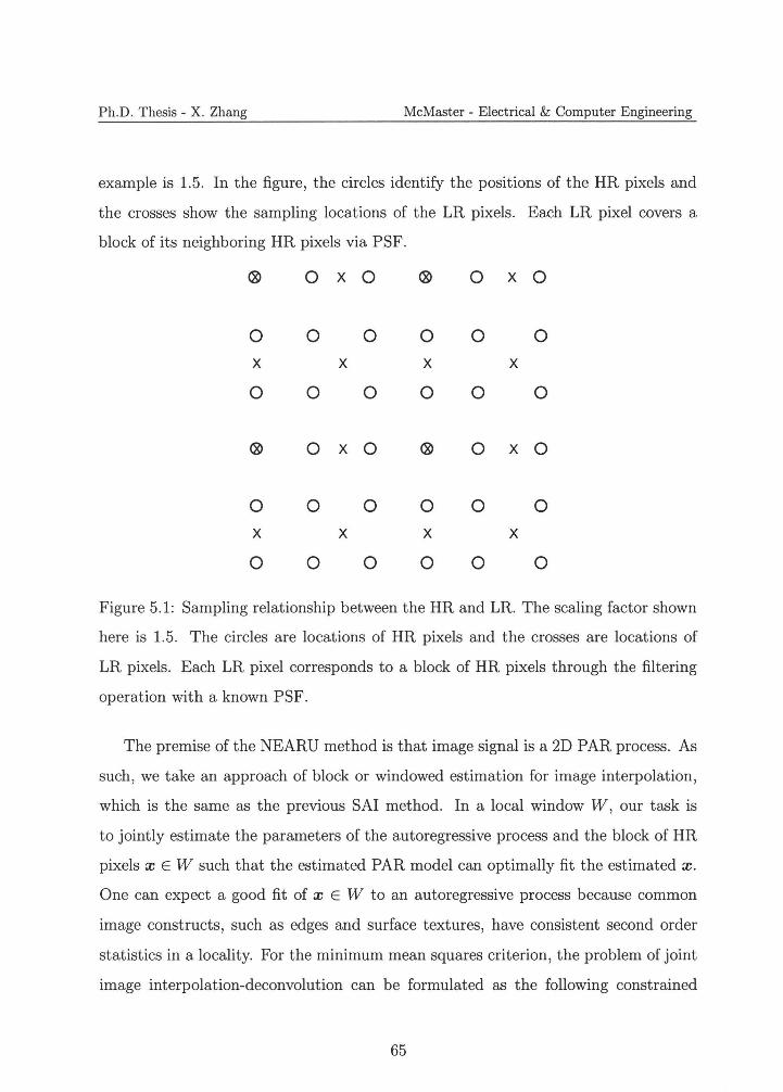
Ph.D. Thesis - X. Zhang McMaster - Electrical & Computer Engineering
example is 1.5. In the figure, the circles identify the positions of the HR pixels and
the crosses show the sampling locations of the LR pixels. Each LR pixel covers a
block of its neighboring HR pixels via PSF.
0 x 0 0 x 0
0 0 0 0 0 0 x x x x
0 0 0 0 0 0
0 x 0 0 x 0
0 0 0 0 0 0 x x x x
0 0 0 0 0 0
Figure 5.1: Sampling relationship between the HR and LR. The scaling factor shown
here is 1.5. The circles are locations of HR pixels and the crosses are locations of
LR pixels. Each LR pixel corresponds to a block of HR pixels through the filtering
operation with a known PSF.
The premise of the NEARU method is that image signal is a 2D PAR process. As
such, we take an approach of block or windowed estimation for image interpolation,
which is the same as the previous SAi method. In a local window W, our task is
to jointly estimate the parameters of the autoregressive process and the block of HR
pixels x E W such that the estimated PAR model can optimally fit the estimated x.
One can expect a good fit of x E W to an autoregressive process because common
image constructs, such as edges and surface textures, have consistent second order
statistics in a locality. For the minimum mean squares criterion, the problem of joint
image interpolation-deconvolution can be formulated as the following constrained
65
Ph.D. Thesis - X. Zhang McMaster - Electrical & Computer Engineering
optimization problem:
2
min L (x(i,j) - Lau,vx(i - u,j :c,a
v)) (i ,j)EW u,v (5.1)
subject to x * h = y
where a is the vector of parameters of a 2D autoregressive model defined in local
window W. The constraints x * h =yin (5.1) correspond to the physical formation
of the LR image via a still camera, where * is the convolution operator, and vector
x consists of all the HR pixels and vector y of all the LR pixels inside window W.
Since the operator* is linear, x * h = y generates L equality constraints, L being the
number of the LR pixels inside W (i.e., the length of vector y).
However, at onset the objective function (5.1) presents a problem of data overfit
ting, or curse of dimensionality. If a PAR model of order t (i.e., the length of vector
a is t) is used, then the number of variables in (5 .1) is JWJ + t, whereas the number
of equations between these variables is only IWI + L. From the spatial configuration
of LR pixels y in relation to HR pixels x, we have L :S l;W. The ratio of the number
of equations versus the number of unknown variables is bounded from above by
IWl(l+-\) 1+-\ 1 ---~°'~= Q <1+- (5.2)
a 2IWI + t 1+ it, 1 1
Since the scaling factor a > 1 for image resolution upconversion, the number of
equations (i.e., the number of samples in the underlying estimation problem) is very
close to the number of unknown variables, almost independent of t. This exposes an
acute data overfitting problem facing NEARU, which cannot be prevented merely by
lowering the order of the PAR model t.
On a second reflection, fortunately, the two dimensions of the image signal afford
us ways to circumvent the problem of data overfitting. One way to increase the
number of equations or constraints on pixels x E W is the use of multiple PAR
models that associate pixels in different directions. Specifically, we introduce two
PAR models of order 4, called the diagonal model ARx and the axial model AR+.
66
Ph.D. Thesis - X. Zhang McMaster - Electrical & Computer Engineering
The models ARx and AR+ act on two disjoint neighborhoods of x(i,j):
s+(i,j) = [x(i,j - 1), x(i - 1,j), x(i, j + 1), x(i + 1, j)f (5.3)
sx(i,j) = [x(i - 1,j - 1), x(i - 1,j + 1), x(i + 1,j + 1), x(i + 1,j - l)f.
Vectors Sx (i, j) and s+(i, j) consist of four 8-connected neighbors and four 4-connected
neighbors of x(i, j) in the HR image, respectively, explaining our terminology of diago
nal and axial models. Incorporating these two PAR models into the original nonlinear
estimation framework, we modify the objective function (5.1) to the following:
min{ L (x(i,j) -xrsx(i,j))2 + L (x(i,j) - 'trs+(i,j)) 2 }
:z:,x;t (i,j)EW (i,j)EW ( 5.4)
subject to x * h = y
where X = (x1, X2, X3, X4) and 't = (r1, T2, T3, T4) are parameters of the two PAR models
ARx and AR+, respectively. From (5.1) to (5.4) the number of equations increases
from IWI + L to 2IWI + L. While the number of equations is almost doubled, the
number of unknown variables increases only by t = 4. Consequently, the ratio of the
number of equations versus the number of unknown variables is increased to
IWl(2 + -\) 2+-\ ----°'~- °' (5.5)
IWI + 8 - 1 + l~I
For example, if the above ratio is required to be 2 for robust estimation, we need to
select a window size IWI ~ 16o:2 . To prevent the overfitting problem, we prefer a
large window W in block estimation of NEARU. However, a large window W has a
higher chance of violating the assumption that the image signal is a stationary AR
process in W . In balance, we choose the window size that makes the above ratio in
the range of 1.5 to 2.
The NEARU framework is general and the regularization term h in (5.4) can be
any degradation function (e.g., PSF compounded by camera motion). To keep this
chapter focused on resolution upconversion we consider only the effect of PSF via
h. The incorporation of PSF in the framework of NEARU unifies the operations of
67
Ph.D. Thesis - X. Zhang McMaster - Electrical & Computer Engineering
image upconversion and deconvolution, which were otherwise performed in two sepa
rate steps in current practice. Unlike many existing image interpolation techniques,
NEARU does not treat the pixels of the LR image as ground truth and will change
these LR pixel values as a result of the non-linear least-squares estimation. Also, since
the constraint x *h = y can accommodate any ratio between the HR and LR image
sizes, NEARU offers a solution of joint upconversion-deconvolution for an arbitrary
scaling factor.
To adapt to possible drifting statistics in image space, the NEARU technique
solves the optimization problem (5.4) in blocks. Adjacent blocks may overlap one the
other to avoid blocking effects. In each local window W, as stipulated by the objective
function (5.4), the parameters of models ARx and AR+ are jointly estimated with
HR pixels x. This is a strategy to circumvent the chicken-and-egg dilemma of having
to use the second order statistics of the LR image to interpolate the HR image, as
proposed in [3]. Since NEARU estimates, in least-squares sense, a whole block of HR
pixels x E W, rather than pixel by pixel in isolation, it is an alternative to Markov
field approach for image interpolation.
Although we adopt two PAR models ARx and AR+ of order 4 only for the sake of
preventing model overfit, the block estimation process of NEARU has the net effect
of an adaptive non-separable two dimensional interpolation filter that has as many
as L taps. Namely, each HR pixel is interpolated using all LR pixels y E W .
5.3 Structured total least-squares solution
By applying a Lagrangian multiplier >., we convert the above constrained nonlinear
least square problem to the following unconstrained nonlinear least square problem:
min{ L (x(i,j)-xTsx(i,j)) 2+ L (x(i,j)--r:I's+(i,j)) 2
:c,x,'t (i,j)EW (i ,j)EW (5.6)
2+ >-1 IY - x *hi 1 }
68
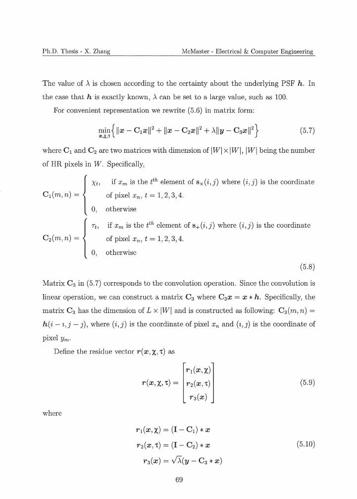
Ph.D. Thesis - X. Zhang McMaster - Electrical & Computer Engineering
The value of A is chosen according to the certainty about the underlying PSF h. In
the case that h is exactly known, A can be set to a large value, such as 100.
For convenient representation we rewrite (5.6) in matrix form:
(5.7)
where C 1 and C 2 are two matrices with dimension of jWj x jWj, jWj being the number
of HR pixels in W. Specifically,
Xt, if Xm is the tth element of s x ( i, j) where ( i, j) is the coordinate
C1(m, n) = of pixel Xn, t = 1, 2, 3, 4.
0, otherwise
Tt, if Xm is the tth element of s+(i,j) where (i,j) is the coordinate
C2(m, n) = of pixel Xn, t = 1, 2, 3, 4.
0, otherwise
(5.8)
Matrix C 3 in (5.7) corresponds to the convolution operation. Since the convolution is
linear operation, we can construct a matrix C 3 where C3x = x *h. Specifically, the
matrix C 3 has the dimension of L x jWj and is constructed as following: C 3 (m, n) =
h(i - i,j - J), where (i,j) is the coordinate of pixel Xn and (i,J) is the coordinate of
pixel Ym·
Define the residue vector r(x, x, -r) as
r1(x,x)l r(x, X, -r) = r2(x, -r) (5.9)
[ r3(x)
where
r1 (x, X) = (I - C1) *x
r2(x, -r) = (I - C2) * x (5.10)
r3(x) = v'>.(y - C3 * x)
69
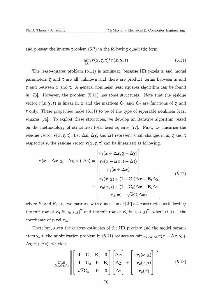
Ph.D. Thesis - X. Zhang McMaster - Electrical & Computer Engineering
and present the inverse problem (5. 7) in the following quadratic form:
min r(x, X, 'tfr(x, X, 't) (5.11):ll,X;t
The least-squares problem (5.11) is nonlinear, because HR pixels x and model
parameters X and 't are all unknown and there are product terms between x and
X and between x and 't. A general nonlinear least squares algorithm can be found
in [75]. However, the problem (5.11) has some structures. Note that the residue
vector r(x, X, 't) is linear in x and the matrices C 1 and C 2 are functions of X and
't only. These properties make (5.11) to be of the type of separable nonlinear least
squares [76]. To exploit these structures, we develop an iterative algorithm based
on the methodology of structured total least squares [77]. First, we linearize the
residue vector r(x, x, 't). Let ~x, ~X, and ~'t represent small changes in x, X and 't
respectively, the residue vector r(x, x, 't) can be linearized as following:
r1(x + ~x, X+ ~X) r(x + ~x, X+ ~X, 't + ~'t) = r 2(x + ~x, 't + ~'t)
T3(X + ~x) (5.12)
r1 (x, X) +(I - C1)~x - E1~Xl r2(x, 't) +(I - C2)~x - E2~'t
[ T3(x) - JXC3~X)
where E 1 and E 2 are two matrices with dimension of !WI x 4 constructed as following:
the mth row of E 1 is sx(i,jf and the mth row of E 2 is s+(i,jf, where (i,j) is the
coordinate of pixel Xm.
Therefore, given the current estimates of the HR pixels x and the model param
eters X, 't, the minimization problem in (5.11) reduces to min.6.:ll,.6.X,.6.t r(x + ~x, X+ ~X, 't + ~'t), which is
2 ~x-l+C1 E1 0 -ri(x,x)
(5 .13)min -I+C2 0 E2 + -r2(x, 't)~x.6.:ll,.6.:x;,.6.t ~'t -r3(x)JXC3 0 0
70
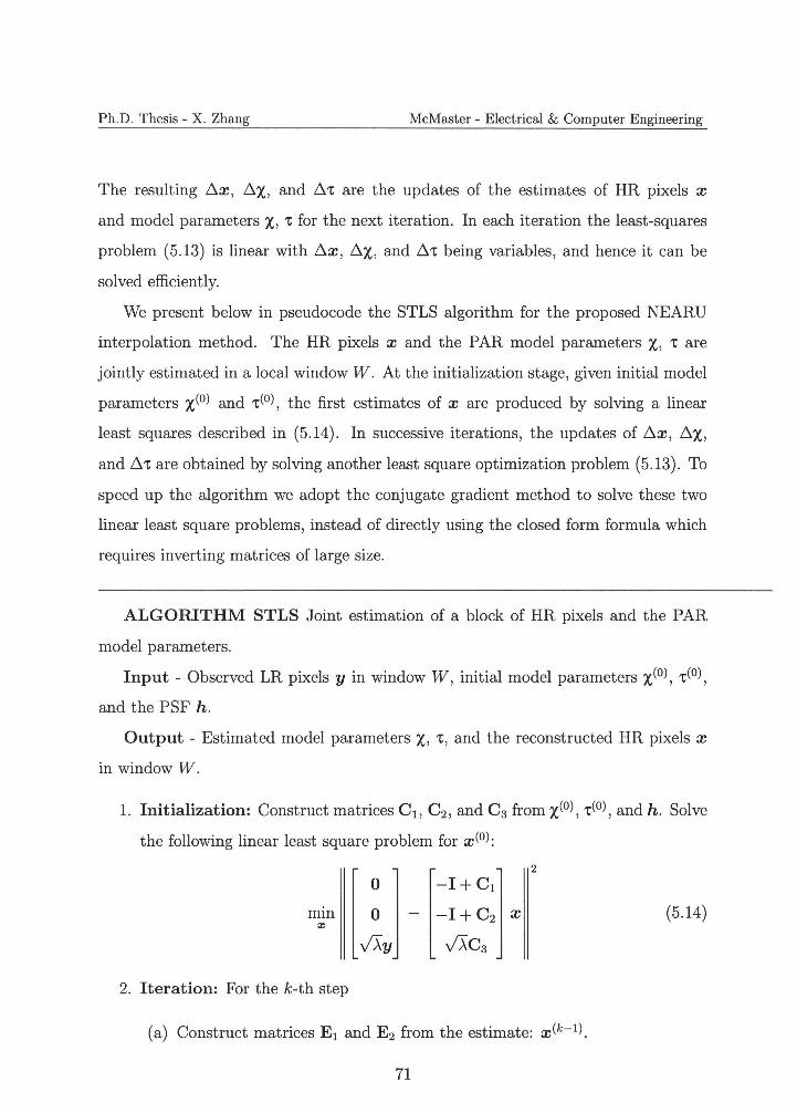
Ph.D. Thesis - X. Zhang McMaster - Electrical & Computer Engineering
The resulting .6.x, .6.x, and .6.'t are the updates of the estimates of HR pixels x
and model parameters X, 't for the next iteration. In each iteration the least-squares
problem (5.13) is linear with .6.x, .6.X, and .6.'t being variables , and hence it can be
solved efficiently.
We present below in pseudocode the STLS algorithm for the proposed NEARU
interpolation method. The HR pixels x and the PAR model parameters x, 't are
jointly estimated in a local window W. At the initialization stage, given initial model
parameters X(o) and 't(o), the first estimates of x are produced by solving a linear
least squares described in (5.14). In successive iterations, the updates of .6.x, .6.x,
and .6.'t are obtained by solving another least square optimization problem (5.13). To
speed up the algorithm we adopt the conjugate gradient method to solve these two
linear least square problems, instead of directly using the closed form formula which
requires inverting matrices of large size.
ALGORITHM STLS Joint estimation of a block of HR pixels and the PAR
model parameters.
Input - Observed LR pixels y in window w, initial model parameters x(O) ' 't(O)'
and the PSF h.
Output - Estimated model parameters X, 't, and the reconstructed HR pixels x
in window W .
1. Initialization: Construct matrices C 1, C 2, and C 3 from X(o), 't(o), and h. Solve
the following linear least square problem for x(o):
2
(5.14)mm O :z:
../Xy
2. Iteration: For the k-th step
(a) Construct matrices E 1 and E 2 from the estimate: x(k-l) .
71
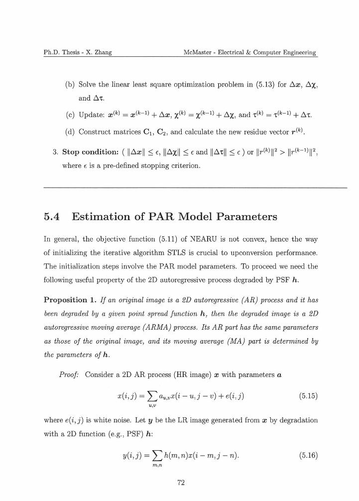
Ph.D. Thesis - X. Zhang McMaster - Electrical & Computer Engineering
(b) Solve the linear least square optimization problem in (5.13) for ~x, ~X,
and ~'t.
(c) Update: x(k) = x(k-l) + ~x, X(k) = X(k-l) + ~X, and 't(k) = 't(k-l) + ~'t.
(d) Construct matrices C 1 , C2 , and calculate the new residue vector r(k).
3. Stop condition: ( ll~xll ~ t, ll~xll ~ t and ll~'tll ~ t) or llr(k) 11 2 > llr(k-1) 11
2,
where t is a pre-defined stopping criterion.
5.4 Estimation of PAR Model Parameters
In general, the objective function (5.11) of NEARU is not convex, hence the way
of initializing the iterative algorithm STLS is crucial to upconversion performance.
The initialization steps involve the PAR model parameters. To proceed we need the
following useful property of the 2D autoregressive process degraded by PSF h.
Proposition 1. If an original image is a 2D autoregressive (AR) process and it has
been degraded by a given point spread function h, then the degraded image is a 2D
autoregressive moving average (ARMA) process. Its AR part has the same parameters
as those of the original image, and its moving average (MA) part is determined by
the parameters of h.
Proof: Consider a 2D AR process (HR image) x with parameters a
x(i,j) = Lau,vx(i - u,j - v) + e(i,j) (5.15) u,v
where e( i, j) is white noise. Let y be the LR image generated from x by degradation
with a 2D function (e.g., PSF) h:
y(i,j) = L h(m,n)x(i - m , j - n). (5.16) m,n
72
Ph.D. Thesis - X. Zhang McMaster - Electrical & Computer Engineering
It follows from
L au,vY(i - u,j - v) = L au,v L h(m, n)x(i - u - m,j - v - n) u,v u,v m,n
= L h(m, n) L au,vx(i - u - m,j - v - n) m,n u ,v
(5.17) = Lh(m,n)(x(i- m,j- n) - e(i-m,j- n))
m ,n
= y(i,j) - Lh(m,n)e(i- m,j - n) m ,n
that y is a 2D ARMA process
y(i,j) = Lau,vY(i- u,j -v) + Lh(m,n)e(i- m,j - n), (5.18) u,v m,n
whose AR part is the same as x and whose MA part is given by h. • The proposition suggests that we can estimate the PAR model parameters X and
't for the original HR pixel block x E W from the observed LR pixel block y E W.
Therefore, we initialize the algorithm STLS by assuming y to be an autoregressive
process of zero mean in local window W. Then by Proposition 1, we compute the
initial PAR model parameters x(O) and 't(O) via the following linear least square esti
mation:
x(O) = argm1n{ L (y(i,J)-xTsx(i,J))2} (i,J)EW
(5.19) 't(o) = argm~in{ L (y(i,J) - 'tTs+(i,J))2
}'
(i,J)EW
where sx(i,J) and s+(i,J) are two four-dimensional vectors whose elements are the
four 8-connected neighbors and four 4-connected neighbors of y(i, J) in the LR image,
respectively. Note that these two vectors only contain the known LR pixels. The
closed form solutions of (5.19) are
x(o) =(ATAt1ATY (5 .20)
't(o) = (BTBtlBTy
73
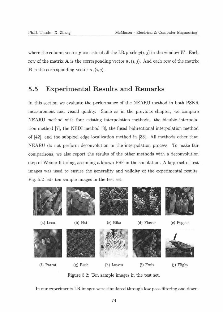
Ph.D. Thesis - X. Zhang McMaster - Electrical & Computer Engineering
where the column vector y consists of all the LR pixels y( i, J) in the window W . Each
row of the matrix A is the corresponding vector sx(i,J). And each row of the matrix
Bis the corresponding vector s+(i,J).
5.5 Experimental Results and Remarks
In this section we evaluate the performance of the NEARU method in both PSNR
measurement and visual quality. Same as in the previous chapter, we compare
NEARU method with four existing interpolation methods: the bicubic interpola
tion method [7], the NEDI method [3], the fused bidirectional interpolation method
of [42], and the subpixel edge localization method in [33]. All methods other than
NEARU do not perform deconvolution in the interpolation process. To make fair
comparisons, we also report the results of the other methods with a deconvolution
step of Weiner filtering , assuming a known PSF in the simulation. A large set of test
images was used to ensure the generality and validity of the experimental results.
Fig. 5.2 lists ten sample images in the test set.
(a) Lena (b) Hat (c) Bike (d) Flower (e) Pepper
(f) Parrot (g) Bush (h) Leaves (i) Fruit (j) Flight
Figure 5.2: Ten sample images in the test set.
In our experiments LR images were simulated through low pass filtering and down
74
Ph.D. Thesis - X. Zhang McMaster - Electrical & Computer Engineering
sampling of the test images. The PSF used in the simulation is a 2D Gaussian filter
with standard deviation of 0.6. Table 5.1 lists the PSNR results of the reconstructed
HR images by the five methods. For the four methods that do not consider PSF
we also include the PSNR values after Wiener deconvolution. Interestingly, Wiener
deconvolution increases the PSNR of the bicubic interpolation method, but it actu
ally decreases the PSNR of the NEDI method and the methods [33, 42] by 3dB or
more. This manifests the deficiency of carrying out interpolation and deconvolution
separately in tandem. On all of the test images the NEARU method outperforms
the others methods without exception. The average gain of NEARU over the second
best method in the group, which is the bicubic method with Wiener deconvolution,
is 1.37 dB.
To assess the visual quality of the NEARU method in comparison with others,
we display in Fig. 5.3 through Fig. 5.6 the output images of the NEARU, NEDI and
bicubic methods on five test images. We include the NEDI method in the visual
comparison group because its perceptual quality is among the best of the previously
published methods. The images produced by the NEDI method look more blurred
than those by the NEARU method for the obvious reason that the former ignores
the effect of PSF. Applying Wiener deconvolution to NEDI sharpens the images but
also generates severe speckle and ringing artifacts, which makes NEDI followed by
deconvolution inferior to NEARU. Similar conclusions can be drawn between the
bicubic interpolation method and NEARU. The NEDI method reproduces large scale
edges noticeably better than the bicubic method, but its performance deteriorates on
edges of high curvature and on small structures. This weakness can be seen by closely
inspecting the eye lashes of Lena (Fig. 5.5( c)) and the writings on the hat (Fig. 5.4( c)).
The new NEARU method appears to be a clear winner in visual quality, preserving
edge geometry well and free of most of the artifacts made by the other methods. The
visual quality assessment results also corroborate the objective measure of PSNR in
Table I.
75
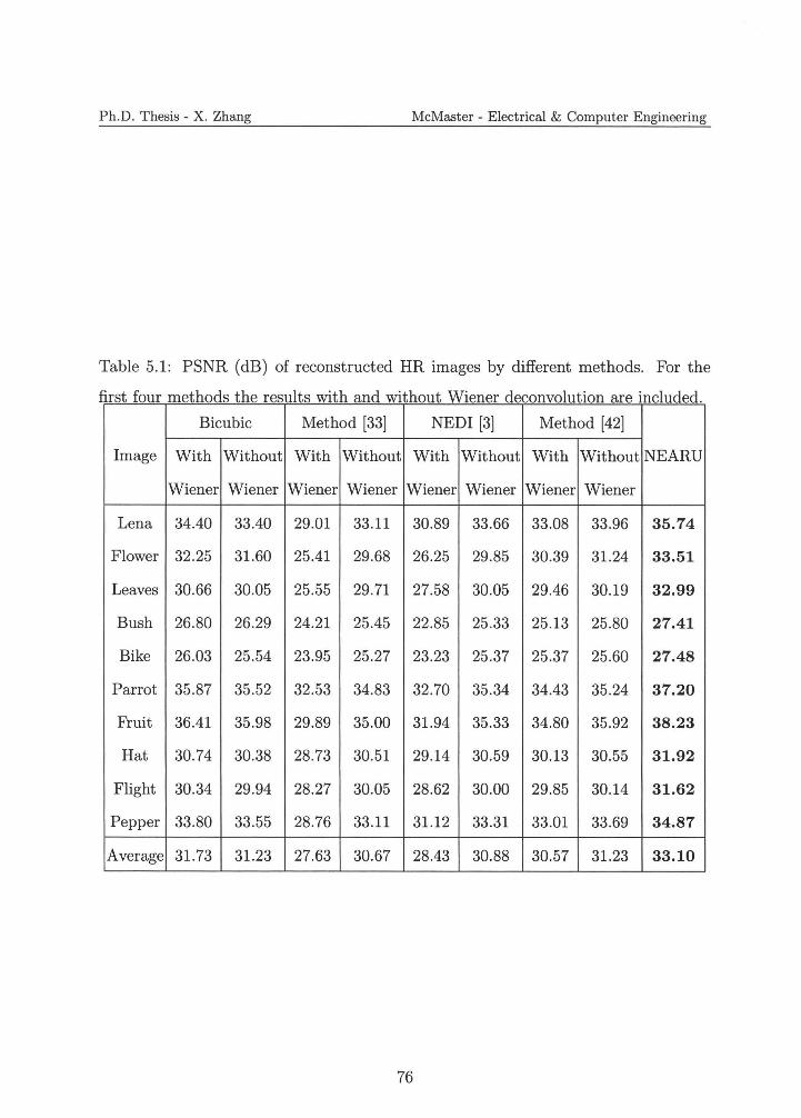
Ph.D. Thesis - X. Zhang McMaster - Electrical & Computer Engineering
Table 5.1: PSNR (dB) of reconstructed HR images by different methods. For the
first four methods the results with and without Wiener deconvolution are included
Bicubic Method [33] NEDI [3] Method [42]
Image With Without With NEARU
Wiener
Without With Without With Without
Wiener Wiener Wiener Wiener Wiener Wiener Wiener
Lena 34.40 33.40 29.01 33.11 30.89 33.66 33.08 33.96 35.74
Flower 32.25 31.60 25.41 29.68 26.25 29 .85 30.39 31.24 33.51
Leaves 30.66 30.05 25.55 29.71 27.58 30.05 29.46 30.19 32.99
Bush 26.80 26.29 24.21 25.45 22.85 25.33 25.13 25.80 27.41
Bike 26.03 25.54 23.95 25.27 23.23 25 .37 25.37 25.60 27.48
Parrot 35.87 35.52 32.53 34.83 32.70 35.34 34.43 35.24 37.20
Fruit 36.41 35.98 29.89 35.00 31.94 35.33 34.80 35.92 38.23
Hat 30.74 30.38 28.73 30.51 29.14 30.59 30.13 30.55 31.92
Flight 30.34 29.94 28.27 30.05 28.62 30.00 29.85 30.14 31.62
Pepper 33.80 33.55 28.76 33.11 31.12 33.31 33.01 33.69 34.87
Average 31.73 31.23 27.63 30.67 28.43 30.88 30.57 31.23 33.10
76
Ph.D. Thesis - X. Zhang McMaster - Electrical & Computer Engineering
An advantage of the proposed NEARU method is its ability to upconvert an image
by an arbitrary scaling factor a. In contrast, with exception of the bicubic interpo
lation method, the other previously published methods were designed to interpolate
images only for scaling factor of power of 2. Therefore, we only compare the NEARU
method with the bicubic method for scaling factors that are not power of 2. Fig. 5.7
and Fig. 5.8 show the interpolated Bike and Hat images by scaling factor of 1.8 and
3.2 respectively. The HR images produced by the NEARU method are visually far
more pleasant than those by the bicubic method followed by Wiener deconvolution,
having cleaner and sharper edges.
We also evaluate the visual quality of different methods for large scaling factors,
a 2: 3. There are applications that demand large scaling factors, such as reproduction
of digital images on magazine cover pages in prepress and on large posters in adver
tisement. Fig. 5.9 shows a part of LR Bike image and its four times magnifications by
the five methods. In this case, the method [33], the NEDI method and the method
[42] are applied twice to perform image resolution upconversion by a factor of four.
As demonstrated by Figs. 5.8 and 5.9, the improvement of the NEARU method over
other methods in perceptual quality becomes even more convincing as scaling factor
a increases. We call readers' attention to the capability of NEARU to faithfully re
produce high curvature edges (e.g., fonts) and large structures alike, free of artifacts
plaguing the other methods.
In the experiments on arbitrary scaling factors, the test images are directly used as
input LR images for the five methods. Here we do not know the true HR images nor
the PSF function h, as in proceeding simulations. Instead, we use a Gaussian PSF
h to associate the input LR with the output HR images in (5.4). In our simulations
the standard deviation a of the Gaussian PSF is made proportional to scaling factor
a, a =ca, c E [0.25, 0.5]. The ratio c = a/a governs the extent of the overlap of PSF
kernels of two adjacent LR pixels. The results shown in Fig. 5.7, Fig. 5.8 and Fig. 5.9
correspond to c = 0.33. In practice, one can adjust the parameter c to control the
77
Ph.D. Thesis - X. Zhang McMaster - Electrical & Computer Engineering
sharpness of the reconstructed HR image. Given the scaling factor a, a PSF of larger
<J (i.e., larger c) will lead to a sharper HR image. Fig. 5.10 illustrates what happens
to the reconstructed HR image when one changes the value of c.
5.6 Conclusion
A technique of model-based nonlinear estimation for adaptive resolution upconver
sion is proposed in this chapter. The image is modeled by two separate piecewise
autoregressive models. The model parameters and the unknown HR pixels are jointly
estimated for an image block. The problem is formulated as a nonlinear least square
optimization problem and a structure total least square based solution is given. The
proposed NEARU technique combines the adaptive upsampling and deconvolution
into one pass and can resize the LR image by an arbitrary scaling factor. The new
technique outperforms the existing techniques in both PSNR measure and subjective
visual quality over a wide range of scenes, and is particularly suitable for large-scale
resolution upconversion.
78
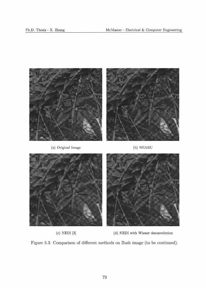
Ph.D. Thesis - X. Zhang McMaster - Electrical & Computer Engineering
(a) Original Image (b) NEARU
(c) NEDI [3] (d) NEDI with Wiener deconvolution
Figure 5.3: Comparison of different methods on Bush image (to be continued).
79
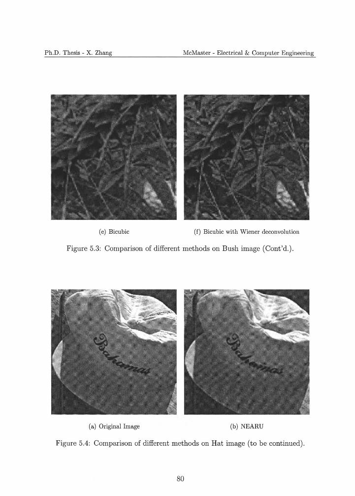
Ph.D. Thesis - X. Zhang McMaster - Electrical & Computer Engineering
(e) Bicubic (f) Bicubic with Wiener deconvolution
Figure 5.3: Comparison of different methods on Bush image (Cont'd.).
(a) Original Image (b) NEARU
Figure 5.4: Comparison of different methods on Hat image (to be continued).
80
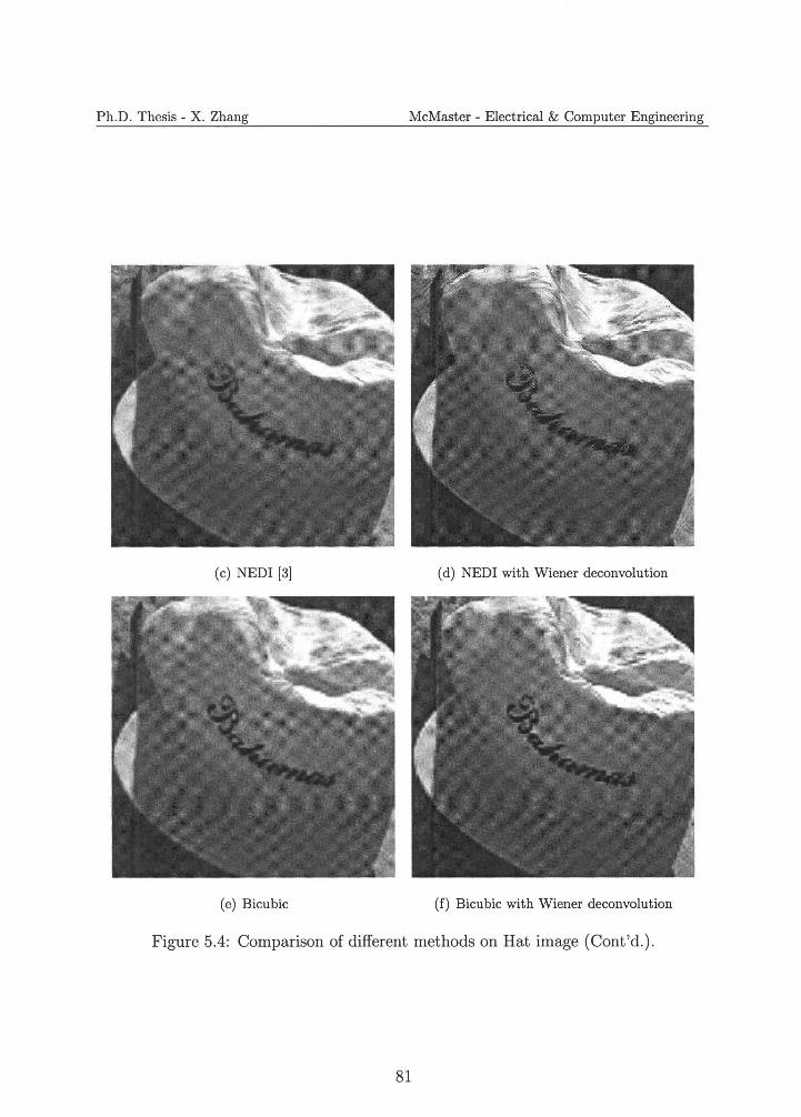
Ph.D. Thesis - X. Zhang McMaster - Electrical & Computer Engineering
(c) NEDI [3] ( d) NEDI with Wiener deconvolution
(e) Bicubic (f) Bicubic with Wiener deconvolution
Figure 5.4: Comparison of different methods on Hat image (Cont'd.).
81
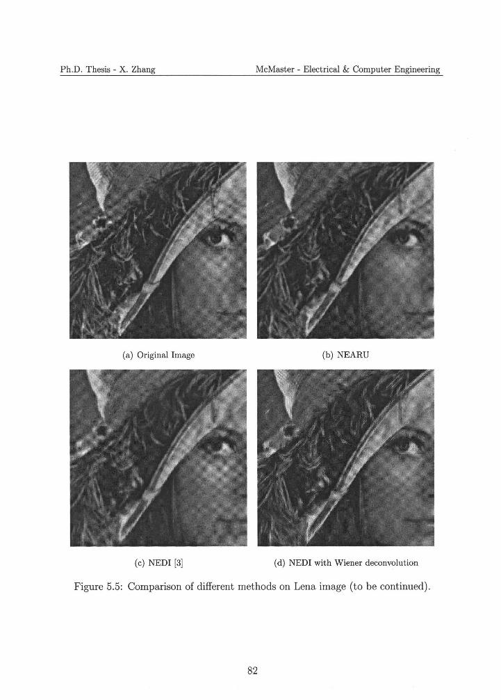
Ph.D. Thesis - X. Zhang McMaster - Electrical & Computer Engineering
(a) Original Image (b) NEARU
(c) NEDI [3] (d) NEDI with Wiener deconvolution
Figure 5.5: Comparison of different methods on Lena image (to be continued).
82
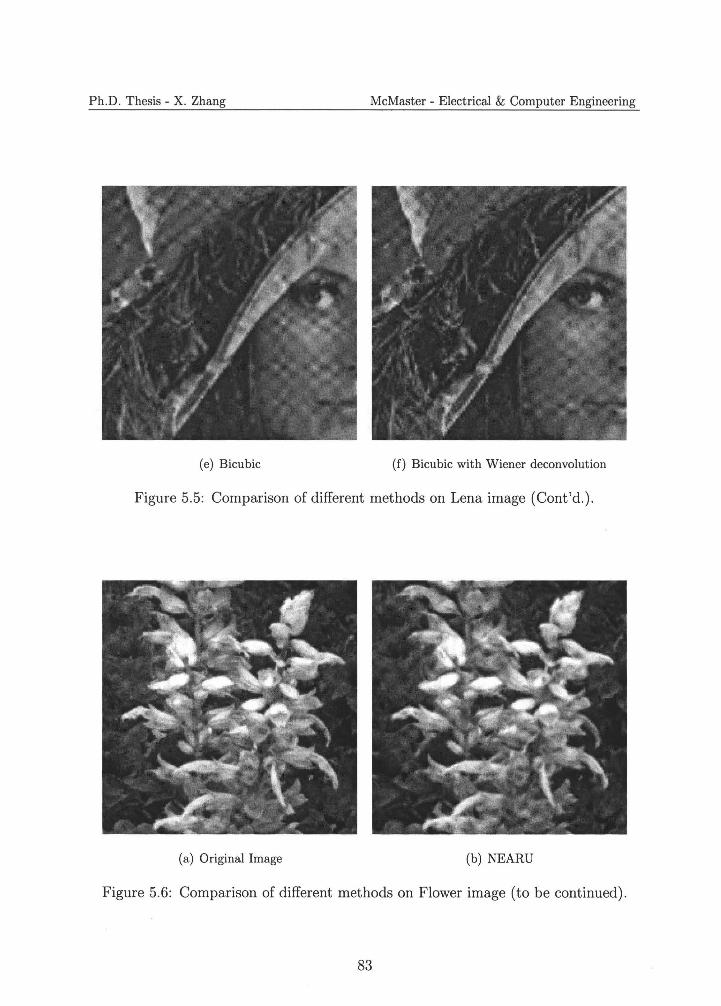
Ph.D. Thesis - X. Zhang McMaster - Electrical & Computer Engineering
(e) Bicubic (f) Bicubic with Wiener deconvolution
Figure 5.5: Comparison of different methods on Lena image (Cont'd.).
(a) Original Image (b) NEARU
Figure 5.6: Comparison of different methods on Flower image (to be continued).
83
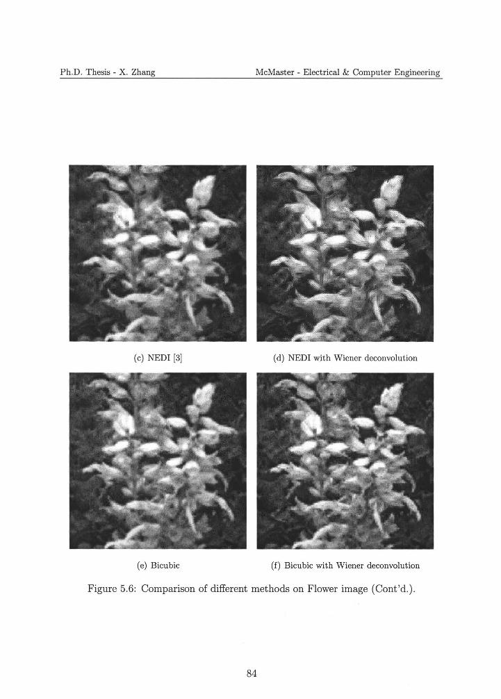
Ph.D. Thesis - X. Zhang McMaster - Electrical & Computer Engineering
(c) NEDI [3] ( d) NEDI wjth Wiener deconvolution
(e) Bicubic (f) Bicubic with Wiener deconvolution
Figure 5.6: Comparison of different methods on Flower image (Cont'd.).
84

Ph.D. Thesis - X. Zhang McMaster - Electrical & Computer Engineering
(a) Bicubic with Wiener deconvolution
Figure 5.7: Interpolated Bike image with scaling factor a= 1.8 (to be continued).
85

Ph.D. Thesis - X. Zhang McMaster - Electrical & Computer Engineering
(b) NEARU
Figure 5.7: Interpolated Bike image with scaling factor a= 1.8 (Cont'd.).
86
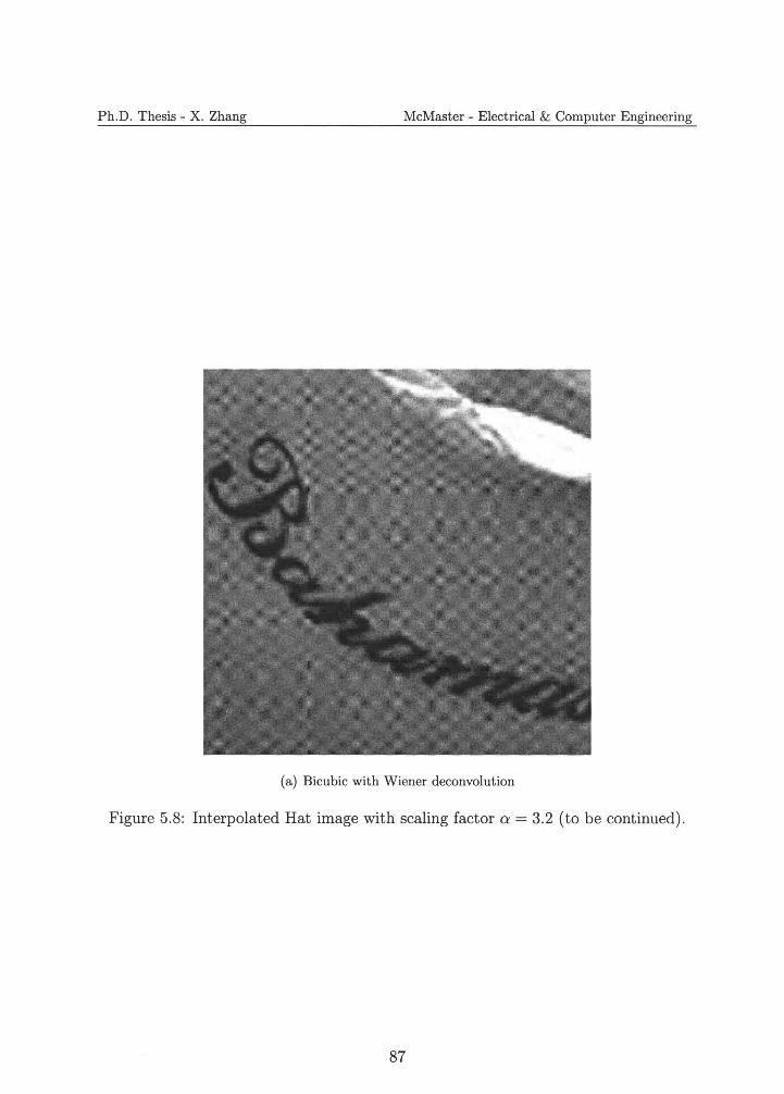
Ph.D. Thesis - X. Zhang McMaster - Electrical & Computer Engineering
(a) Bicubic with Wiener deconvolution
Figure 5.8: Interpolated Hat image with scaling factor a= 3.2 (to be continued).
87

Ph.D. Thesis - X. Zhang McMaster - Electrical & Computer Engineering
(b) NEARU
Figure 5.8: Interpolated Hat image with scaling factor a= 3.2 (Cont'd.).
88
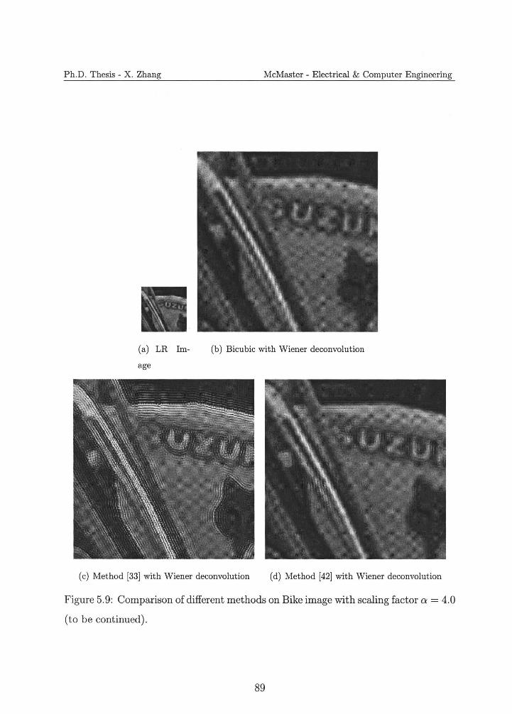
Ph.D. Thesis - X. Zhang McMaster - Electrical & Computer Engineering
(a) LR Im (b) Bicubic with Wiener deconvolution
age
(c) Method [33] with Wiener deconvolution (d) Method [42] with Wiener deconvolution
Figure 5.9: Comparison of different methods on Bike image with scaling factor a= 4.0
(to be continued).
89
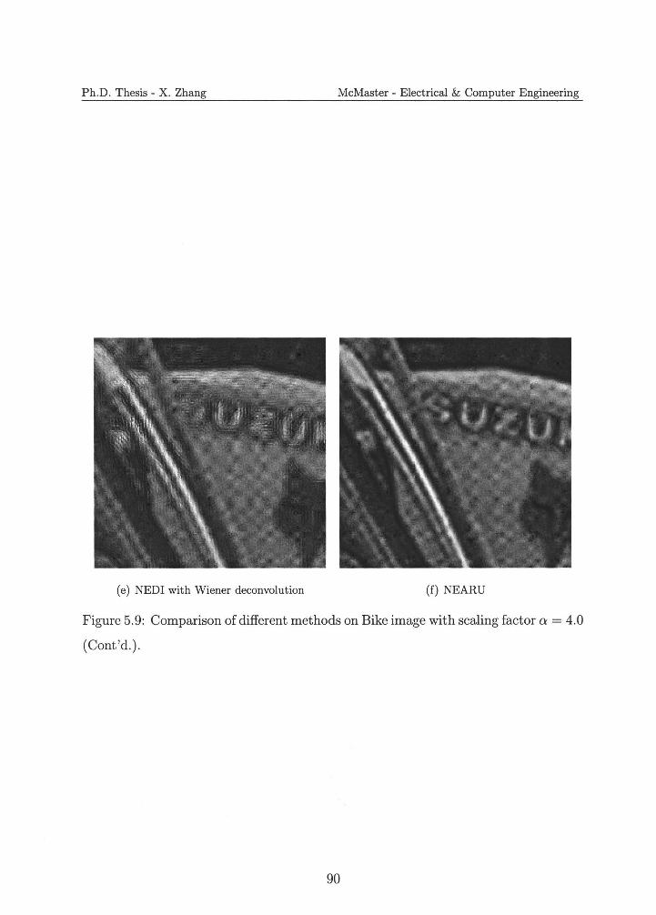
Ph.D. Thesis - X. Zhang McMaster - Electrical & Computer Engineering
(e) NEDI with Wiener deconvolution (f) NEARU
Figure 5.9: Comparison of different methods on Bike image with scaling factor a= 4.0
(Cont'd.).
90
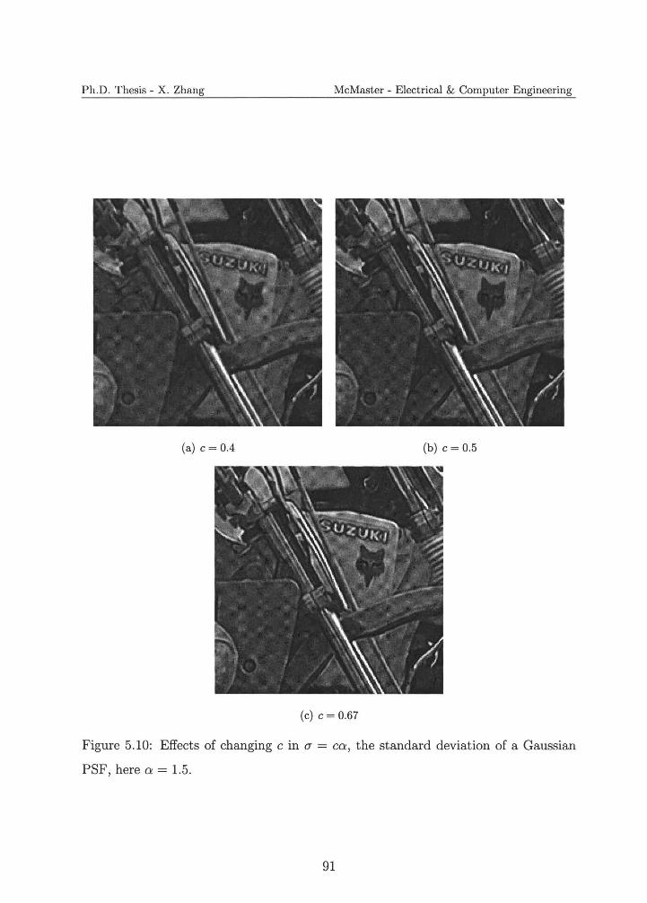
Ph.D. Thesis - X. Zhang McMaster - Electrical & Computer Engineering
(a) c = 0.4 (b) c = 0.5
(c) c = 0.67
Figure 5.10: Effects of changing c in <7 = ca, the standard deviation of a Gaussian
PSF, here a= 1.5.
91
Ph.D. Thesis - X. Zhang McMaster - Electrical & Computer Engineering
Chapter 6
Compression by Collaborative
Adaptive Down-sampling and
Upconversion
In the remainder of this thesis our attention is turned to the use of image inter
polation as a tool for low bit-rate image compression. In this chapter we study
interpolation-based image compression of single description, and extend this work to
multiple descriptions in the next chapter.
6.1 Overview
Over the past half century the prevailing engineering practice of image/video com
pression, as exemplified by all existing image and video compression standards, is to
start with a dense 2D sample grid of pixels. Compression is done by transforming the
spatial image signal into a space (e.g., spaces of Fourier or wavelet bases) in which
the image has a sparse representation and by entropy coding of transform coefficients.
Recently, researchers in the emerging field of compressive sensing challenged the wis
dom of what they called "oversampling followed massive dumping" approach. They
92
Ph.D. Thesis - X. Zhang McMaster - Electrical & Computer Engineering
showed, quite surprisingly, it is possible, at least theoretically, to obtain compact
signal representation by a greatly reduced number of random samples [78].
In this chapter, we seek for compact image representation in an approach of sparse
sampling in the spatial domain. The fact that most natural images have an exponen
tially decaying power spectrum suggests the possibility of interpolation-based com
pact representation of images. A typical scene contains predominantly smooth regions
that can be satisfactorily interpolated from a sparsely sampled low-resolution image.
The difficulty is with the reconstruction of high frequency contents. Of particular
importance is faithful reconstruction of edges without large phase errors, which is
detrimental to perceptual quality of a decoded image.
To answer the above challenge, we develop a new image compression methodol
ogy of collaborative adaptive down-sampling and upconversion. The CADU approach
puts an emphasis on edge reconstruction for the perceptual importance of edges and
also to exploit the anisotropy of edge spectrum. In the CADU encoder design we
choose not to perform uneven irregular down sampling of an input image according
to local spatial or frequency characteristics. Instead, we stick to conventional square
pixel grid by uniform spatial down sampling of the image. Consequently, the re
sulting LR image can be readily compressed by any of existing image compression
techniques, such as DCT-based JPEG and JPEG 2000. Yet the simple uniform down
sampling scheme is made adaptive by a directional low-pass prefiltering step prior to
down-sampling. The other purpose of this preprocessing is to induce a mechanism of
collaboration between the spatial uniform down-sampling process at the encoder and
optimal upconversion process at the decoder.
The CADU decoder first decompresses the LR image and then upconverts it to
the original resolution in constrained least squares restoration process, using a 2D
PAR model, which is similar to the interpolation method described in previous chap
ter. Two-dimensional autoregressive modeling was a known effective technique of
predictive image coding [72, 79]. For the CADU decoder, the PAR model plays a role
93
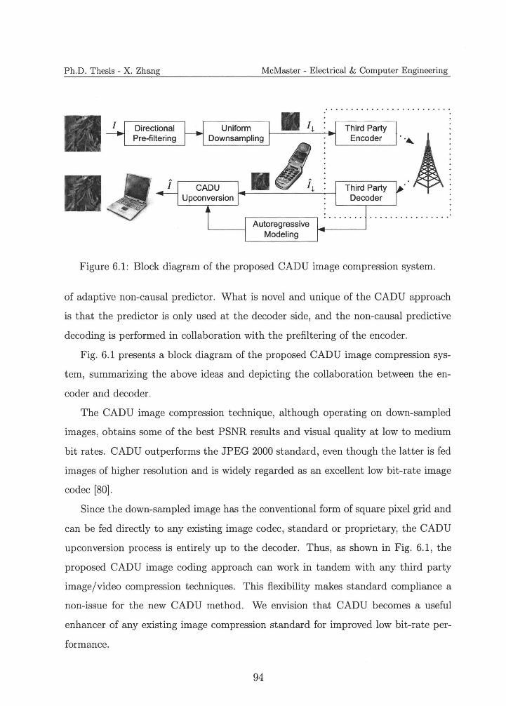
Ph.D. Thesis - X. Zhang McMaster - Electrical & Computer Engineering
II Directional Pre-filtering
-~
• /J,Uniform Downsampling
.I,,CADU
Upconversion
Autoregressive Modeling
Third Party Encoder ..._
Third Party Decoder
Figure 6.1: Block diagram of the proposed CADU image compression system.
of adaptive non-causal predictor. What is novel and unique of the CADU approach
is that the predictor is only used at the decoder side, and the non-causal predictive
decoding is performed in collaboration with the prefiltering of the encoder.
Fig. 6.1 presents a block diagram of the proposed CADU image compression sys
tem, summarizing the above ideas and depicting the collaboration between the en
coder and decoder.
The CADU image compression technique, although operating on down-sampled
images, obtains some of the best PSNR results and visual quality at low to medium
bit rates. CADU outperforms the JPEG 2000 standard, even though the latter is fed
images of higher resolution and is widely regarded as an excellent low bit-rate image
codec [80] .
Since the down-sampled image has the conventional form of square pixel grid and
can be fed directly to any existing image codec, standard or proprietary, the CADU
upconversion process is entirely up to the decoder. Thus, as shown in Fig. 6.1, the
proposed CADU image coding approach can work in tandem with any third party
image/video compression techniques. This flexibility makes standard compliance a
non-issue for the new CADU method. We envision that CADU becomes a useful
enhancer of any existing image compression standard for improved low bit-rate per
formance.
94
Ph.D. Thesis - X. Zhang McMaster - Electrical & Computer Engineering
An important application of CADU is visual communication in wireless networks,
where the bandwidth is at a premium and end devices have diverse display capa
bilities, ranging from small screens of cell phones to regular screens of laptops. As
illustrated in Fig. 6.1, the same standard-compliant code stream 11 feeds displays
of different resolutions. The only difference is that high-resolution displays invoke
CADU upconversion while low-resolution displays do not. This design happens to be
compatible with network hardware levels since high-resolution displays are typically
associated with more powerful computers. In such a heterogenous wireless environ
ment scalable or layered image compression methods (e.g., JPEG 2000) are inefficient ,
because the refinement portion of the scalable code stream still consumes bandwidth
and yet generates no benefits to low-resolution devices.
Because the down-sampled image is only a small fraction of the original size,
CADU greatly reduces the encoder complexity, regardless what third-party codec
is used in conjunction. This property allows the system to shift the computation
burden from the encoder to decoder, making CADU a viable asymmetric compression
solution when the encoder is resource deprived. Furthermore, the superior low bit-rate
performance of the CADU approach seems to suggest that a camera of unnecessarily
high resolution can ironically produce inferior images than a lower resolution camera,
if given a tight bit budget. This rather counter-intuitive observation should be heeded
when one designs visual communication devices/systems with severe constraints of
energy and bandwidth.
The related previous works were reviewed in Section 2.3 of Chapter 2. Those
works were largely motivated by the susceptibility of DCT-based block codecs to
severe artifacts at low bit rates. However, in our view, for applications of very tight
bit budget , one should adopt wavelet-based codecs, such as JPEG 2000, which are
well known for their clear superiority over DCT-based codecs in both subjective and
objective quality at low bit rates. Now the question is whether it is also advantageous
to downsample an image prior to wavelet-based compression at low bit rates. This
95
Ph.D. Thesis - X. Zhang McMaster - Electrical & Computer Engineering
chapter will answer this question affirmatively. In fact, according to our experimental
results, the CADU technique coupled with JPEG 2000 consistently has higher PSNR
than all existing techniques for bit rates below 0.3 bpp, and it achieves better visual
quality than others for bit rates up to 0.5 bpp.
The chapter is organized as follows. Section 6.2 describes the CADU encoder of
uniform down-sampling with adaptive direction prefiltering. Section 6.3 presents the
restoration process in decoder: a constrained least squares upconversion algorithm
driven by a PAR image model. We report and discuss the experimental results in
Section 6.4.
6.2 Uniform Down-Sampling with Adaptive Direc
tional Prefiltering
Out of practical considerations, we make a more compact representation of an image
by decimating every other row and every other column of the image. This sim
ple approach has an operational advantage that the down-sampled image remains a
uniform rectilinear grid of pixels, and can readily be compressed by any of existing
international image coding standards. To prevent the down-sampling process from
causing aliasing artifacts, it seems necessary to low-pass pre-filter an input image to
half of its maximum frequency !max· However, on a second reflection, one can do
somewhat better. In areas of edges, the 2D spectrum of the local image signal is
not isotropic. Thus we seek to perform adaptive sampling, within the uniform down
sampling framework, by judiciously smoothing the image with directional low-pass
prefiltering prior to down-sampling.
To this end, we design a family of 2D directional low-pass prefilters under the
criterion of preserving the maximum 2D bandwidth without the risk of aliasing. Let
wL(B) and WH(B) be the side lengths of the rectangular low-passed region of the 2D
filter in the low- and high-frequency directions of an edge of angle e, respectively.
96
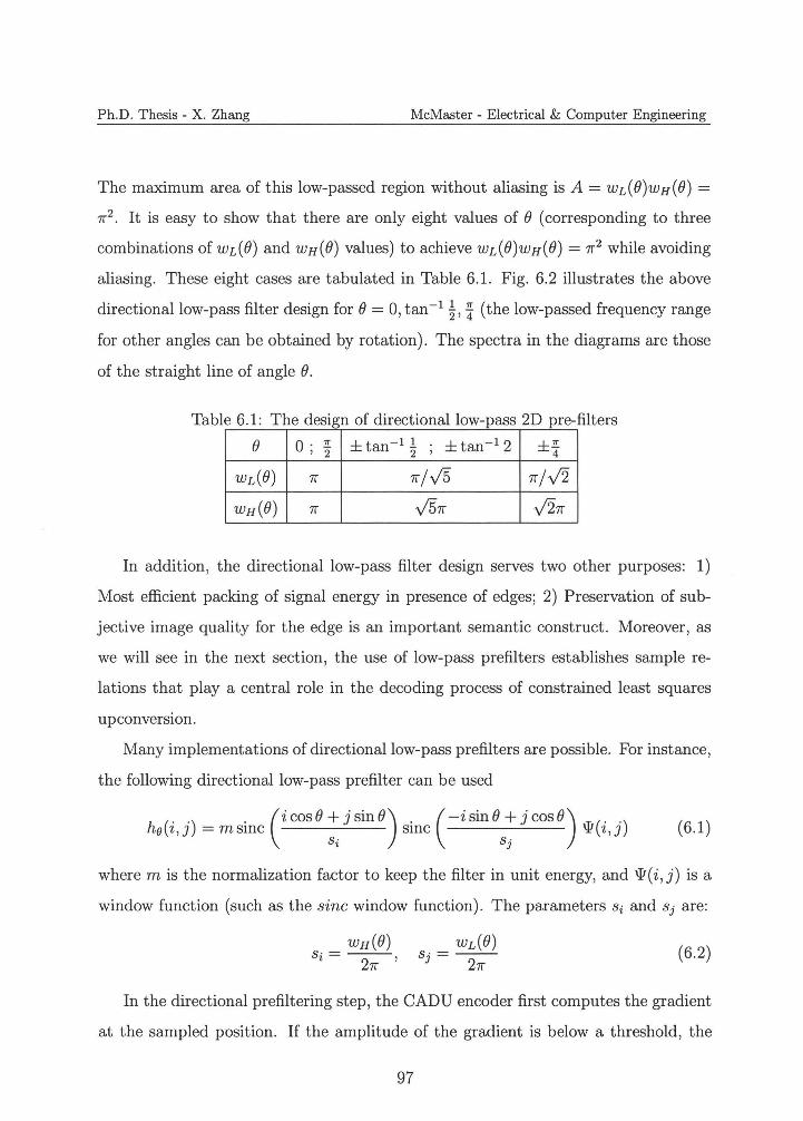
Ph.D. Thesis - X. Zhang McMaster - Electrical & Computer Engineering
The maximum area of this low-passed region without aliasing is A= wL(O)wH(O) =
7r2. It is easy to show that there are only eight values of () (corresponding to three
combinations of wL(O) and wH(O) values) to achieve wL(O)wH(O) = 7r2 while avoiding
aliasing. These eight cases are tabulated in Table 6.1. Fig. 6.2 illustrates the above
directional low-pass filter design for()= 0, tan-1 !, ~ (the low-passed frequency range
for other angles can be obtained by rotation). The spectra in the diagrams are those
of the straight line of angle ().
Table 6.1: The design of directional low-pass 2D pre-filters
() 0. Z!:. , 2 ± tan-1 l
2 · ±tan-1 2, ±Z!:.
4
WL(()) 7r 7r/V5 7r/../2 WH(O) 7r V57r ../27r
In addition, the directional low-pass filter design serves two other purposes: 1)
Most efficient packing of signal energy in presence of edges; 2) Preservation of sub
jective image quality for the edge is an important semantic construct . Moreover, as
we will see in the next section, the use of low-pass prefilters establishes sample re
lations that play a central role in the decoding process of constrained least squares
upconversion.
Many implementations of directional low-pass prefilters are possible. For instance,
the following directional low-pass prefilter can be used
h ( ..) . ( icosO +jsinO) . (-isinO+jcosO) ff·(· .)e i,J = msmc smc 'i' i,J (6.1) Si Sj
where mis the normalization factor to keep the filter in unit energy, and w(i,j) is a
window function (such as the sine window function). The parameters Si and Sj are:
WH(O) WL(O)s·--- (6.2)Si= 2;-' J - 27r
In the directional prefiltering step, the CADU encoder first computes the gradient
at the sampled position. If the amplitude of the gradient is below a threshold, the
97
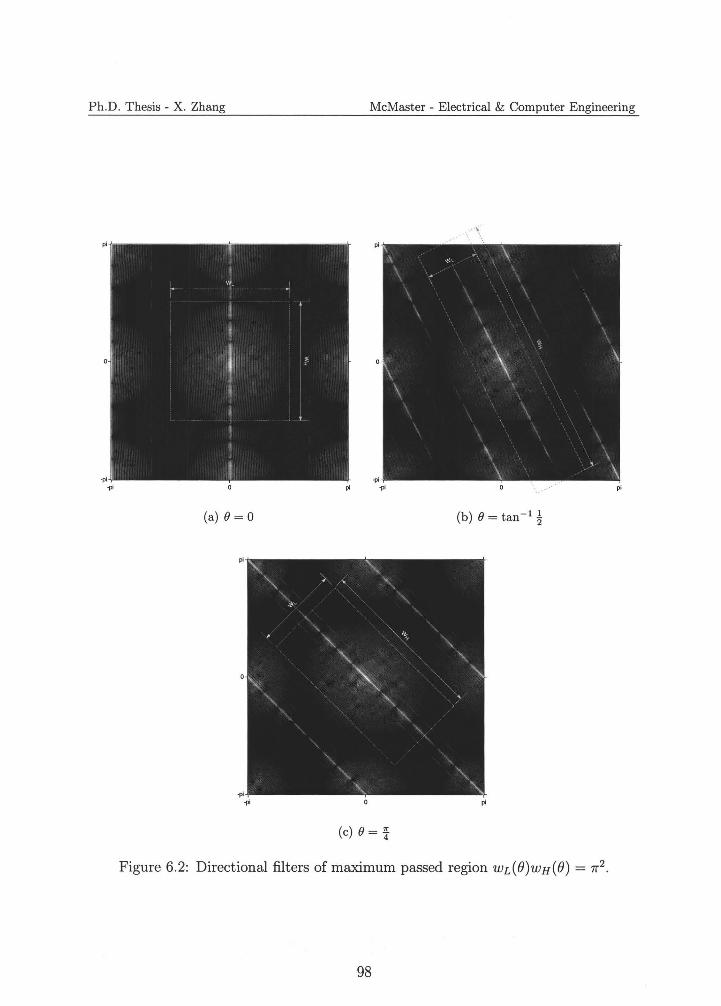
Ph.D. Thesis - X. Zhang McMaster - Electrical & Computer Engineering
(a) B = 0 (b) () = tan- 1 ~
(c) () = %
Figure 6.2: Directional filters of maximum passed region wL(O)wH(O) = 7r2 .
98
Ph.D. Thesis - X. Zhang McMaster - Electrical & Computer Engineering
isotropic low-pass filter h 0 is applied. Otherwise, the gradient direction is quantized
and the corresponding filter ho in Table 6.1 is selected and applied.
Despite its simplicity, the CADU compression approach via uniform down-sampling
is not inherently inferior to other image compression techniques in rate-distortion per
formance, as long as the target bit rate is below a threshold. The argument is based
on the classical water-filling principle in rate-distortion theory. To encode a set of
K independent Gaussian random variables {X1,X2 , • · · ,XK}, Xk ,....., N(O,ak), the
rate-distortion bounds, when the total bit rate being R = L,~=l Rk and the total
mean-squares distortion being D = L,~=l Dk, are given by
K { 1 2}R(D) ={;max 0, 2log2 ;
(6.3)K
D(R) = I:min{r,aD k=l
Most natural images have a rapidly (e.g., exponentially) decaying power spectrum
<I>(w). Suppose that the input image is i.i.d. in the Fourier domain and its power
spectrum is monotonically decreasing. Therefore, given a target rate r*, if the rate
distortion function of the image signal satisfies
D(r*) > 11r <I>(w)dw, (6.4) 7r/2
then uniform down-sampling by the factor of two will not limit the rate-distortion
performance in information theoretical sense. Indeed, our experimental results (see
Section 6.4) demonstrate that the CADU approach outperforms the state-of-the-art
JPEG 2000 standard in the low to medium bit rate range.
6.3 Constrained Least Squares Upconversion with
Autoregressive Modeling
In this section we develop the decoder of the CADU image compression system. Let
Ji be the decompressed ~ x 1¥- subsampled image, and I be the original M x N image.
99
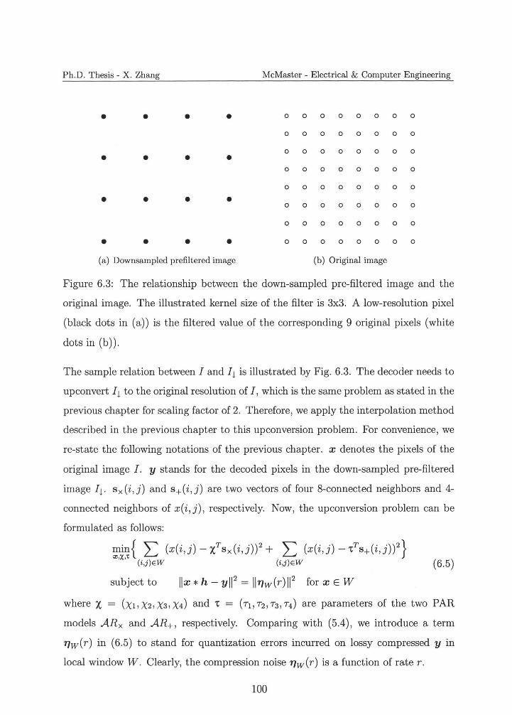
• • • •
• • • •
• • • •
• • • •
Ph.D. Thesis - X. Zhang McMaster - Electrical & Computer Engineering
0 0 0 0 0 0 0 0
0 0 0 0 0 0 0 0
0 0 0 0 0 0 0 0
0 0 0 0 0 0 0 0
0 0 0 0 0 0 0 0
0 0 0 0 0 0 0 0
0 0 0 0 0 0 0 0
0 0 0 0 0 0 0 0
(a) Downsampled prefiltered image (b) Original image
Figure 6.3: The relationship between the down-sampled pre-filtered image and the
original image. The illustrated kernel size of the filter is 3x3. A low-resolution pixel
(black dots in (a)) is the filtered value of the corresponding 9 original pixels (white
dots in (b)).
The sample relation between I and I 1 is illustrated by Fig. 6.3. The decoder needs to
upconvert I1 to the original resolution of I, which is the same problem as stated in the
previous chapter for scaling factor of 2. Therefore, we apply the interpolation method
described in the previous chapter to this upconversion problem. For convenience, we
re-state the following notations of the previous chapter. x denotes the pixels of the
original image I. y stands for the decoded pixels in the down-sampled pre-filtered
image I 1. sx(i , j) and s+(i,j) are two vectors of four 8-connected neighbors and 4
connected neighbors of x(i,j), respectively. Now, the upconversion problem can be
formulated as follows:
min{ 2:= (x(i,j)-xTsx(i,j)) 2+ 2:= (x(i,j)--cTs+(i,j))2}:i:,x,i:
(i,j)EW (i,j)EW ( 6.5)
subject to llx *h - Yll 2 = ll11w(r)ll 2 for x E W
where X = (x1 , x2 , x3 , x4 ) and "C = (T1 , Tz, T3 , T4 ) are parameters of the two PAR
models ARx and AR+, respectively. Comparing with (5.4), we introduce a term
1Jw(r) in (6.5) to stand for quantization errors incurred on lossy compressed y in
local window W . Clearly, the compression noise 1Jw(r) is a function of rater.
100
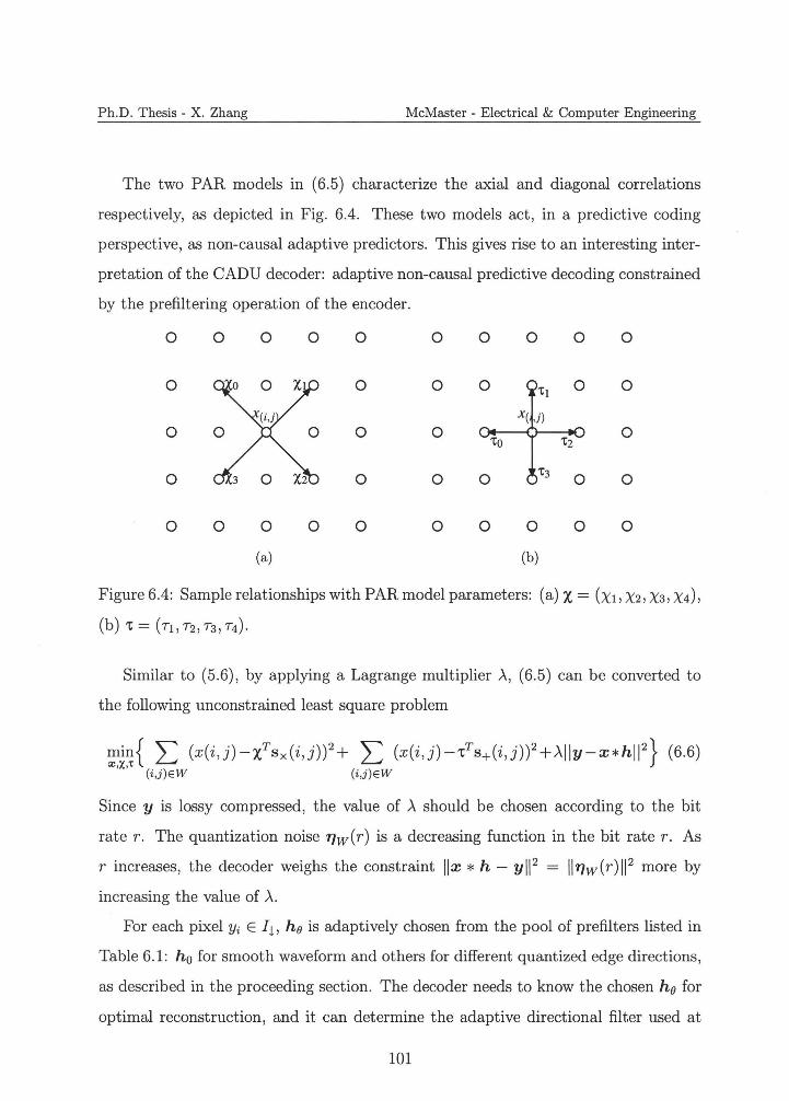
Ph.D. Thesis - X. Zhang McMaster - Electrical & Computer Engineering
The two PAR models in (6.5) characterize the axial and diagonal correlations
respectively, as depicted in Fig. 6.4. These two models act, in a predictive coding
perspective, as non-causal adaptive predictors. This gives rise to an interesting inter
pretation of the CADU decoder: adaptive non-causal predictive decoding constrained
by the prefiltering operation of the encoder.
0 0 0 0 0 0 0 0 0 0
0 0 0 0 0 0'tt
0 0 0 'to 't2
't30 0 0 0 0
0
0
0 0 0 0 0 0 0 0 0 0
(a) (b)
Figure 6.4: Sample relationships with PAR model parameters: (a) x = (x1,x2,x3,X4),
(b) 't = (r1,T2,T3,T4).
Similar to (5.6), by applying a Lagrange multiplier .A, (6.5) can be converted to
the following unconstrained least square problem
Since y is lossy compressed, the value of A should be chosen according to the bit
rate r . The quantization noise '11w(r) is a decreasing function in the bit rater . As
r increases, the decoder weighs the constraint llx * h - Yll 2 = 11'17w(r)ll 2 more by
increasing the value of .A.
For each pixel Yi E 11, ho is adaptively chosen from the pool of prefilters listed in
Table 6.1: ho for smooth waveform and others for different quantized edge directions,
as described in the proceeding section. The decoder needs to know the chosen ho for
optimal reconstruction, and it can determine the adaptive directional filter used at
101
Ph.D. Thesis - X. Zhang McMaster - Electrical & Computer Engineering
the encoder by applying the same gradient operator as the encoder to the decoded
image J1. This achieves the synchronization of the encoder and decoder with high
probability without sending any side information.
The CADU system design is asymmetric: the encoder is a simple and inexpensive
process, while the decoder involves solving a rather large-scale optimization problem
described in (6.6).
6.4 Experimental Results and Discussions
The proposed image coding method was implemented and evaluated in both PSNR
and subjective quality. We compared the CADU method with the adaptive downsampling
based image codec proposed by Lin and Dong [67]. The latter was reportedly the best
among all previously published downsampling-interpolation image codecs [63, 64] in
both objective and subjective quality. Note that all existing image codecs of this
type were developed for DCT-based image compression, whereas the CADU method
is applicable to wavelet-based codecs as well. Therefore, we also include in our com
parative study JPEG 2000, the quincunx coding method [81], and the method of
uniform down-sampling at the encoder and bicubic interpolation at the decoder. The
bicubic method in the comparison group and the CADU method used the same sim
ple encoder: JPEG 2000 coding of uniformly down-sampled prefiltered image. The
difference is in the upconversion process: the former method performed bicubic im
age interpolation followed by a deconvolution step using Weiner filter to reverse the
prefiltering, instead of solving a constrained least squares image restoration problem
driven by autoregressive models as described in the proceeding section.
Although the proposed CADU method favors the reconstruction of edges, we
chose, for fairness and generality of our comparative study, a large set of test images
of various scene compositions. Here we report experimental results for four repre
sentative images, which represent all common image features in balance: edges of all
102
Ph.D. Thesis - X. Zhang McMaster - Electrical & Computer Engineering
scales, smooth regions, and granular textures, as one can see in Fig. 6.5.
Table 6.2 lists the PSNR results of seven methods: DCT-based old JPEG stan
dard (column JPEG), the method of Lin and Dong [67] (the 2nd column), the CADU
method coupled with DCT-based JPEG (column CADU-JPG) JPEG 2000 (column
J2K), JPEG 2000 coupled with uniform downsampling and bicubic interpolation (col
umn Bicubic), the quincunx method [81] (column Quincunx), and the CADU method
coupled with JPEG 2000 (column CADU-J2K). The results are tabulated against var
ious bit rates from 0.1 bpp to 0.3 bpp. For the first two methods of the group, some
table entries at very low bit rates are "N/A" because the DCT-based JPEG cannot
even operate at such low rates for the image tested.
The PSNR comparison between Lin-Dong's method and the CADU-JPG method
is somewhat mixed. CADU-JPG has a small advantage over Lin-Dong's method in
most cases, but the former lost to the latter by small margin for test images Flower and
Bike when the rate is equal to and greater than 0.25 bpp. Although these two methods
outperform old JPEG without downsampling, but they both produced significantly
lower PSNR than wavelet-based JPEG 2000 without downsampling. Obviously, one
should use JPEG 2000 when the bit budget is low in practice. For the state of the art
in low bit rate image compression, the reader should pay closer attention to the results
of the wavelet group in Table 6.2. At low rates, the CADU-J2K method achieves up
to 0.5 dB higher PSNR than JPEG 2000. This improvement is quite remarkable given
that JPEG 2000 is highly regarded for its outstanding performance at low rates [2].
Among the four competing methods in the wavelet group, the bicubic interpolation
method has the lowest PSNR in most cases. Given that the CADU-J2K and bicubic
interpolation methods use the same prefilters and the same JPEG 2000 encoder, the
performance gap between the two manifests the efficacy of least squares non-causal
predictive decoding constrained by adaptive directional low-pass prefiltering.
The quincunx coding method also outperforms JPEG 2000 at low to modest bit
rates, but it requires a much more expensive, non-standard encoder.
103
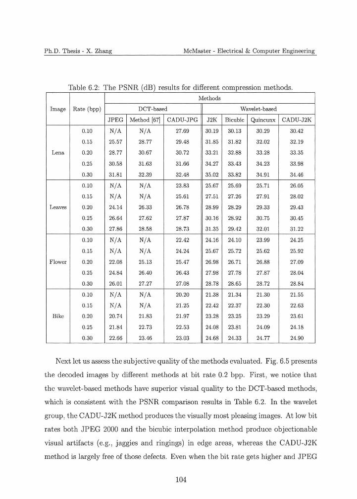
Ph.D. Thesis - X. Zhang McMaster - Electrical & Computer Engineering
Table 6.2: The PSNR (dB) results for different compression methods. Methods
Image Rate (bpp) DCT-based Wavelet-based
JPEG Method [67] CADU-JPG J2K Bicubic Quincunx CADU-J2K
0.10
0.15
N/A
25.57
N/A
28.77
27.69
29.48
30.19
31.85
30.13
31.82
30.29
32.02
30.42
32.19
Lena 0.20 28.77 30.67 30.72 33.21 32.88 33.28 33.35
0.25 30.58 31.63 31.66 34.27 33.43 34.23 33.98
0.30 31.81 32.39 32.48 35.02 33.82 34.91 34.46
Leaves
0.10
0.15
0.20
N/A
N/A
24.14
N/A
N/A
26.33
23.83
25.61
26.78
25.67
27.51
28.99
25.69
27.26
28.29
25.71
27.91
29.33
26.05
28.02
29.43
0.25 26.64 27.62 27.87 30.16 28.92 30.75 30.45
0.30 27.86 28.58 28.73 31.35 29.42 32.01 31.22
Flower
0.10
0.15
0.20
N/A
N/A
22.08
N/A
N/A
25.13
22.42
24.24
25.47
24.16
25.67
26.98
24.10
25.72
26.71
23.99
25.62
26.88
24.25
25.92
27.09
0.25 24.84 26.40 26.43 27.98 27.78 27.87 28.04
0.30 26.01 27.27 27.08 28.78 28.65 28.72 28.84
Bike
0.10
0.15
0.20
N/A
N/A
20.74
N/A
N/A
21.83
20.20
21.25
21.97
21.38
22.42
23.28
21.34
22.37
23.25
21.30
22.30
23.29
21.55
22.63
23.61
0.25 21.84 22.73 22.53 24.08 23.81 24.09 24.18
0.30 22.66 23.46 23.03 24.68 24.33 24.77 24.90
Next let us assess the subjective quality of the methods evaluated. Fig. 6.5 presents
the decoded images by different methods at bit rate 0.2 bpp. First, we notice that
the wavelet-based methods have superior visual quality to the DCT-based methods,
which is consistent with the PSNR comparison results in Table 6.2. In the wavelet
group, the CADU-J2K method produces the visually most pleasing images. At low bit
rates both JPEG 2000 and the bicubic interpolation method produce objectionable
visual artifacts (e.g., jaggies and ringings) in edge areas, whereas the CADU-J2K
method is largely free of those defects. Even when the bit rate gets higher and JPEG
104
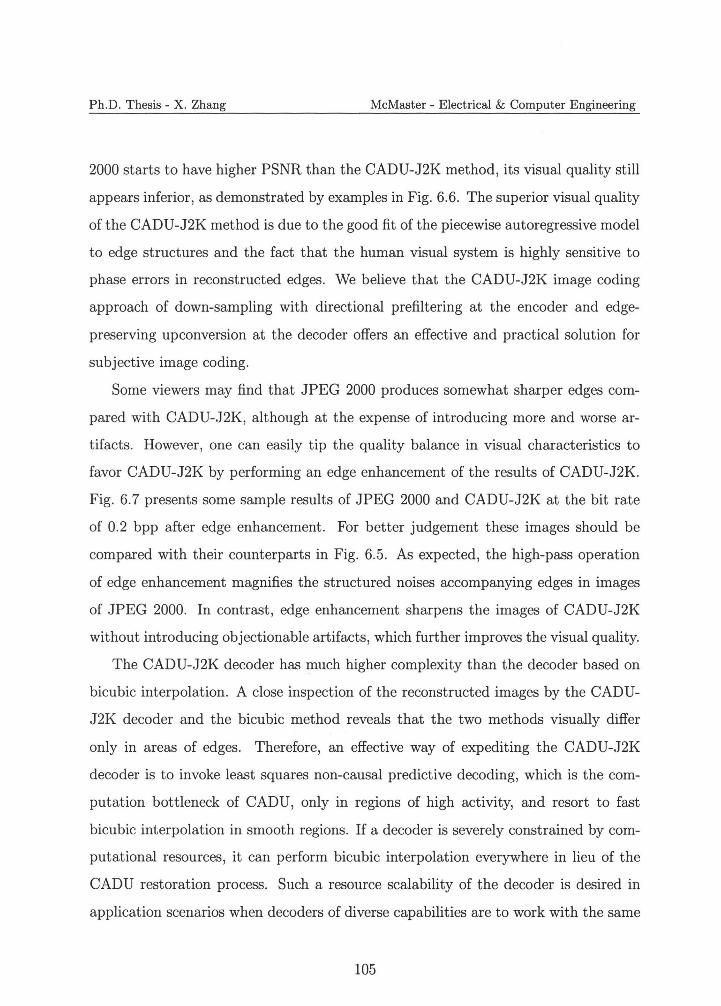
Ph.D. Thesis - X. Zhang McMaster - Electrical & Computer Engineering
2000 starts to have higher PSNR than the CADU-J2K method, its visual quality still
appears inferior, as demonstrated by examples in Fig. 6.6. The superior visual quality
of the CADU-J2K method is due to the good fit of the piecewise autoregressive model
to edge structures and the fact that the human visual system is highly sensitive to
phase errors in reconstructed edges. We believe that the CADU-J2K image coding
approach of down-sampling with directional prefiltering at the encoder and edge
preserving upconversion at the decoder offers an effective and practical solution for
subjective image coding.
Some viewers may find that JPEG 2000 produces somewhat sharper edges com
pared with CADU-J2K, although at the expense of introducing more and worse ar
tifacts. However, one can easily tip the quality balance in visual characteristics to
favor CADU-J2K by performing an edge enhancement of the results of CADU-J2K.
Fig. 6. 7 presents some sample results of JPEG 2000 and CADU-J2K at the bit rate
of 0.2 bpp after edge enhancement. For better judgement these images should be
compared with their counterparts in Fig. 6.5. As expected, the high-pass operation
of edge enhancement magnifies the structured noises accompanying edges in images
of JPEG 2000. In contrast, edge enhancement sharpens the images of CADU-J2K
without introducing objectionable artifacts, which further improves the visual quality.
The CADU-J2K decoder has much higher complexity than the decoder based on
bicubic interpolation. A close inspection of the reconstructed images by the CADU
J2K decoder and the bicubic method reveals that the two methods visually differ
only in areas of edges. Therefore, an effective way of expediting the CADU-J2K
decoder is to invoke least squares non-causal predictive decoding, which is the com
putation bottleneck of CADU, only in regions of high activity, and resort to fast
bicubic interpolation in smooth regions. If a decoder is severely constrained by com
putational resources, it can perform bicubic interpolation everywhere in lieu of the
CADU restoration process. Such a resource scalability of the decoder is desired in
application scenarios when decoders of diverse capabilities are to work with the same
105
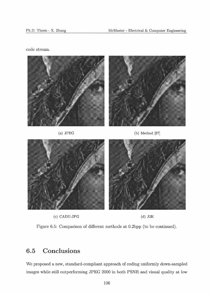
Ph.D. Thesis - X. Zhang McMaster - Electrical & Computer Engineering
code stream.
(a) JPEG (b) Method [67]
(c) CADU-JPG (d) J2K
Figure 6.5: Comparison of different methods at 0.2bpp (to be continued).
6.5 Conclusions
We proposed a new, standard-compliant approach of coding uniformly down-sampled
images while still outperforming JPEG 2000 in both PSNR and visual quality at low
106

Ph.D. Thesis - X. Zhang McMaster - Electrical & Computer Engineering
to modest bit rates. This success is due to the novel upconversion process of least
square non-causal predictive decoding constrained by adaptive directional low-pass
prefiltering. Our findings suggest that a lower sampling rate can actually produce
higher quality images at certain bit rates.
107
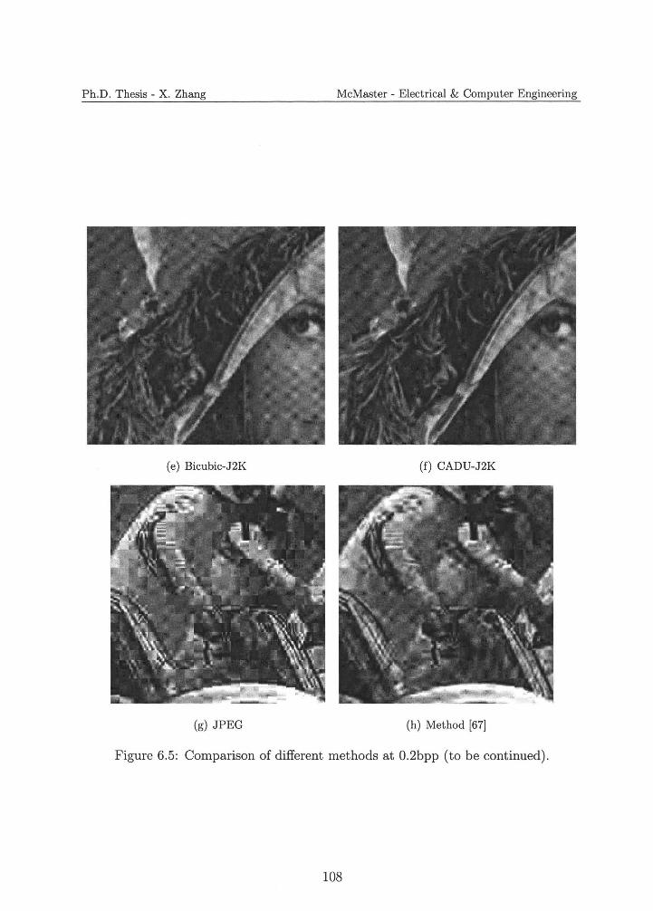
Ph.D. Thesis - X. Zhang McMaster - Electrical & Computer Engineering
(e) Bicubic-J2K (f) CADU-J2K
(g) JPEG (h) Method [67]
Figure 6.5: Comparison of different methods at 0.2bpp (to be continued) .
108
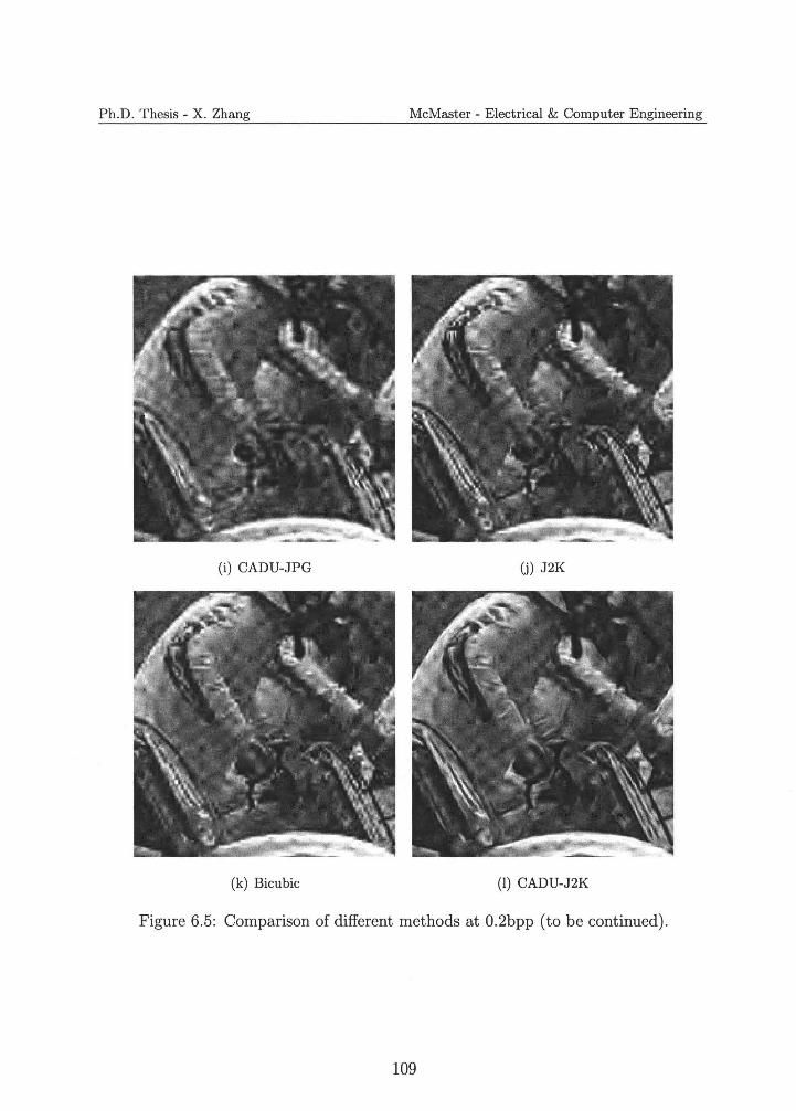
Ph.D. Thesis - X. Zhang McMaster - Electrical & Computer Engineering
(i) CADU-JPG (j) J2K
(k) Bicubic (1) CADU-J2K
Figure 6.5: Comparison of different methods at 0.2bpp (to be continued).
109
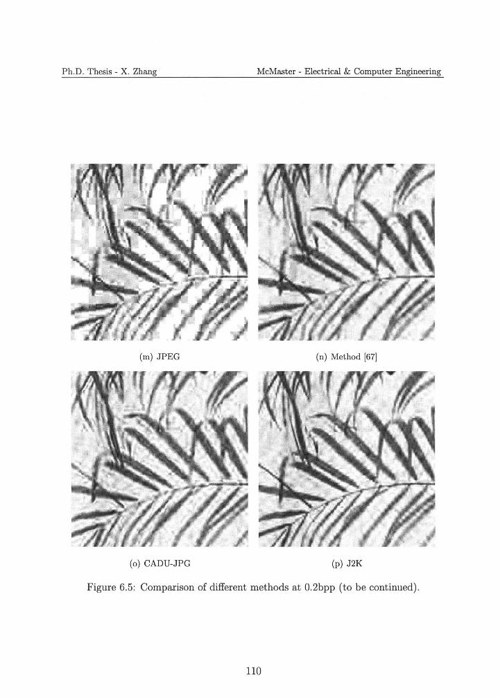
Ph.D. Thesis - X. Zhang McMaster - Electrical & Computer Engineering
(m) JPEG (n) Method [67]
(o) CADU-JPG (p) J2K
Figure 6.5: Comparison of different methods at 0.2bpp (to be continued) .
110
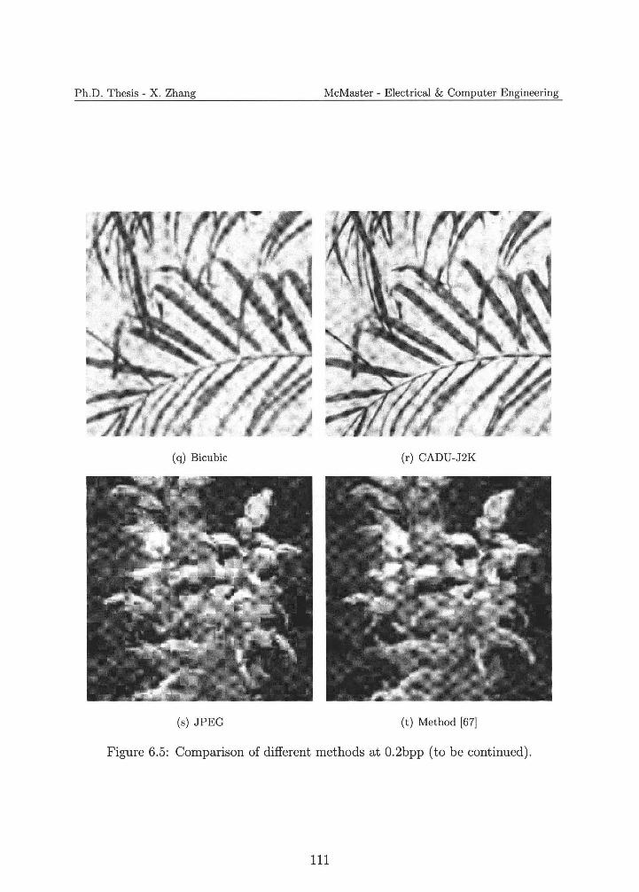
Ph.D. Thesis - X. Zhang McMaster - Electrical & Computer Engineering
(q) Bicubic (r) CADU-J2K
(s) JPEG (t) Method [67]
Figure 6.5: Comparison of different methods at 0.2bpp (to be continued).
111
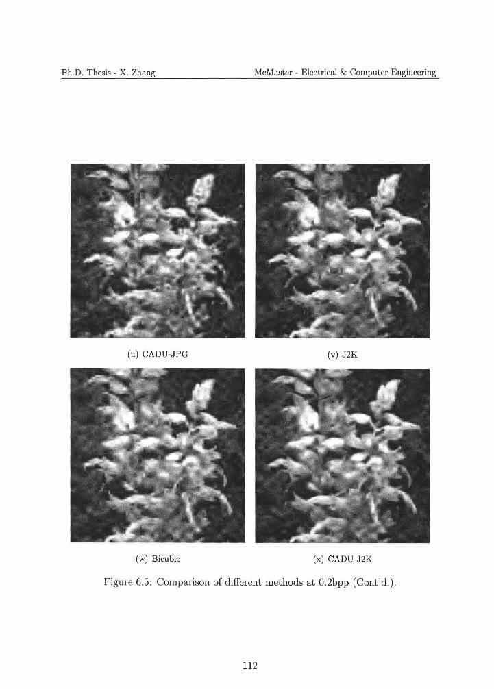
Ph.D. Thesis - X. Zhang McMaster - Electrical & Computer Engineering
(u) CADU-JPG (v) J2K
(w) Bicubic (x) CADU-J2K
Figure 6.5: Comparison of different methods at 0.2bpp (Cont'd.) .
112
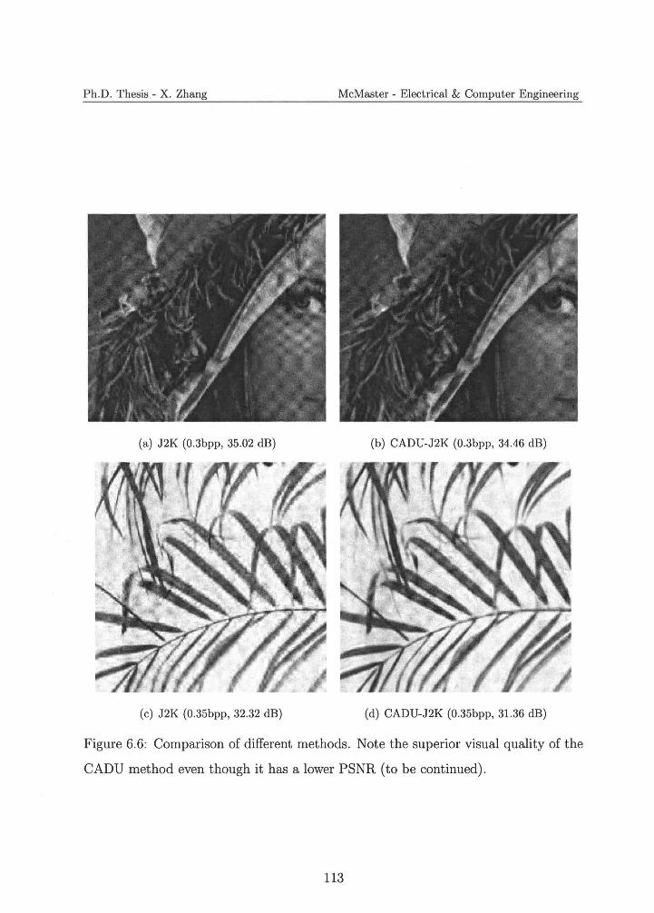
Ph.D. Thesis - X. Zhang McMaster - Electrical & Computer Engineering
(a) J2K (0.3bpp, 35.02 dB) (b) CADU-J2K (0.3bpp, 34.46 dB)
(c) J2K (0.35bpp, 32.32 dB) (d) CADU-J2K (0.35bpp, 31.36 dB)
Figure 6.6: Comparison of different methods. Note the superior visual quality of the
CADU method even though it has a lower PSNR (to be continued).
113
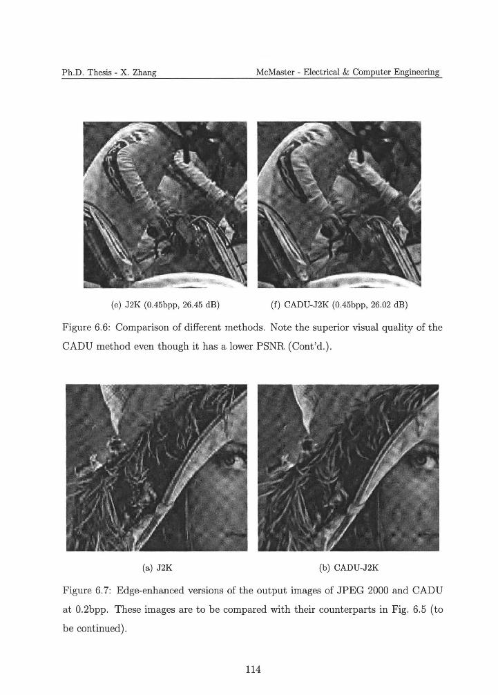
Ph.D. Thesis - X. Zhang McMaster - Electrical & Computer Engineering
(e) J2K (0.45bpp, 26.45 dB) (f) CADU-J2K (0.45bpp, 26.02 dB)
Figure 6.6: Comparison of different methods. Note the superior visual quality of the
CADU method even though it has a lower PSNR (Cont 'd .).
(a) J2K (b) CADU-J2K
Figure 6. 7: Edge-enhanced versions of the output images of JPEG 2000 and CADU
at 0.2bpp. These images are to be compared with their counterparts in Fig. 6.5 (to
be continued).
114
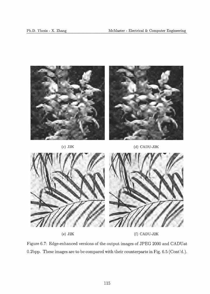
Ph.D. Thesis - X. Zhang McMaster - Electrical & Computer Engineering
(c) J2K (d) CADU-J2K
(e) J2K (f) CADU-J2K
Figure 6.7: Edge-enhanced versions of the output images of JPEG 2000 and CADUat
0.2bpp. These images are to be compared with their counterparts in Fig. 6.5 (Cont'd.).
115
Ph.D. Thesis - X. Zhang McMaster - Electrical & Computer Engineering
Chapter 7
Spatial Multiplexing Multiple
Description Coding
In this chapter, we extend our study on interpolation-based image compression from
conventional single description coding to multiple description coding , and propose
a practical standard-compliant image MDC technique. Multiple descriptions of an
image are generated in the spatial domain by an adaptive prefiltering and uniform
down sampling process, similar to the CADU approach described in the previous
chapter. The resulting side descriptions are conventional square sample grids that
are interleaved with one the other. As such each side description can be coded by
any of the existing image compression standards. The side decoder is same as the
decoder in CADU approach. The central decoder is algorithmically similar to the side
decoder, but it improves the reconstruction quality by using received side descriptions
as additional constraints when solving the underlying inverse problem.
7.1 Overview
One of the landmarks of modern digital multimedia technology is ubiquitous vi
sual communications over lossy public networks (e.g., the Internet). The needs for
116
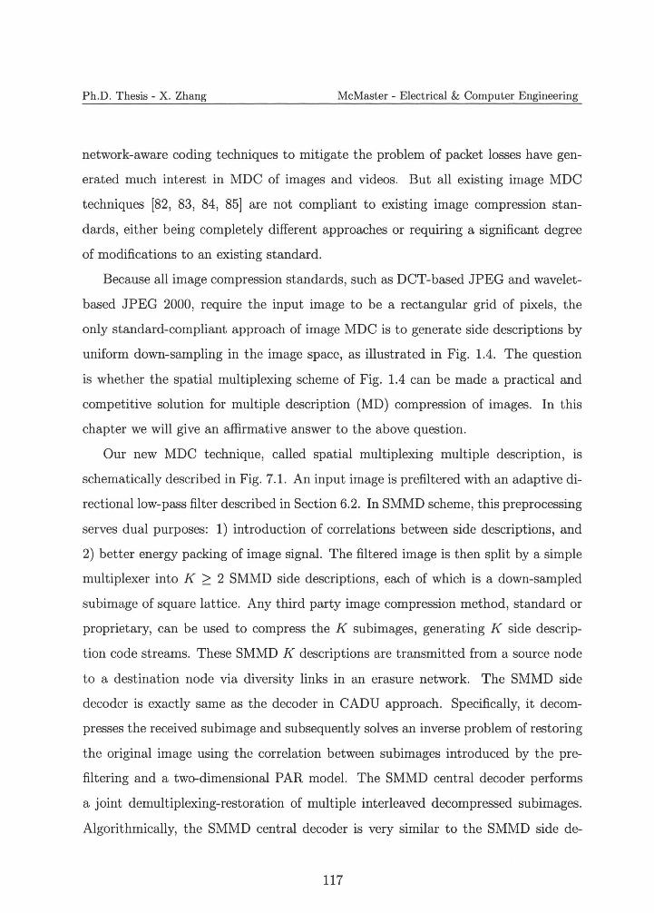
Ph.D. Thesis - X. Zhang McMaster - Electrical & Computer Engineering
network-aware coding techniques to mitigate the problem of packet losses have gen
erated much interest in MDC of images and videos. But all existing image MDC
techniques [82, 83, 84, 85] are not compliant to existing image compression stan
dards, either being completely different approaches or requiring a significant degree
of modifications to an existing standard.
Because all image compression standards, such as DCT-based JPEG and wavelet
based JPEG 2000, require the input image to be a rectangular grid of pixels, the
only standard-compliant approach of image MDC is to generate side descriptions by
uniform down-sampling in the image space, as illustrated in Fig. 1.4. The question
is whether the spatial multiplexing scheme of Fig. 1.4 can be made a practical and
competitive solution for multiple description (MD) compression of images. In this
chapter we will give an affirmative answer to the above question.
Our new MDC technique, called spatial multiplexing multiple description, is
schematically described in Fig. 7.1. An input image is prefiltered with an adaptive di
rectional low-pass filter described in Section 6.2. In SMMD scheme, this preprocessing
serves dual purposes: 1) introduction of correlations between side descriptions, and
2) better energy packing of image signal. The filtered image is then split by a simple
multiplexer into K ~ 2 SMMD side descriptions, each of which is a down-sampled
subimage of square lattice. Any third party image compression method, standard or
proprietary, can be used to compress the K subimages, generating K side descrip
tion code streams. These SMMD K descriptions are transmitted from a source node
to a destination node via diversity links in an erasure network. The SMMD side
decoder is exactly same as the decoder in CADU approach. Specifically, it decom
presses the received subimage and subsequently solves an inverse problem of restoring
the original image using the correlation between subimages introduced by the pre
filtering and a two-dimensional PAR model. The SMMD central decoder performs
a joint demultiplexing-restoration of multiple interleaved decompressed subimages.
Algorithmically, the SMMD central decoder is very similar to the SMMD side de
117
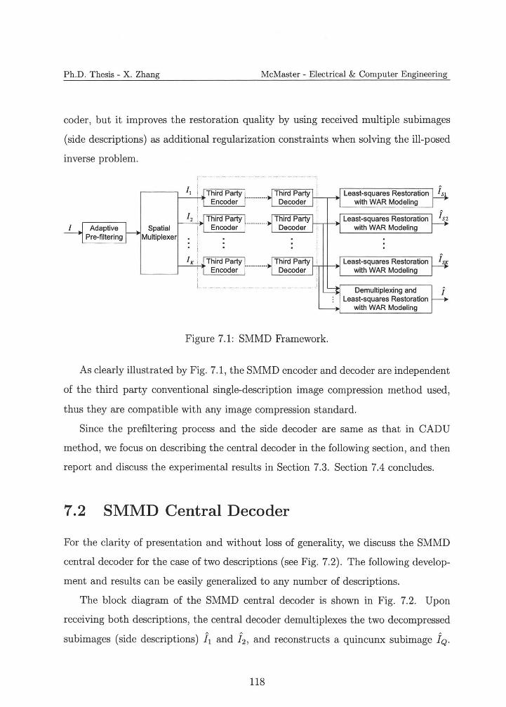
Ph.D. Thesis - X. Zhang McMaster - Electrical & Computer Engineering
coder, but it improves the restoration quality by using received multiple subimages
(side descriptions) as additional regularization constraints when solving the ill-posed
inverse problem.
I Adaptive Pre-filtering
Spatial Multiplexer
Third Party Encoder
Least-squares Restoration is with WAR Modeling
Least-squares Restoration isi with WAR Modeling
Least-squares Restoration is with WAR Modeling
Demultiplexing and i Least-squares Restoration
with WAR Modeling
Figure 7.1 : SMMD Framework.
As clearly illustrated by Fig. 7.1, the SMMD encoder and decoder are independent
of the third party conventional single-description image compression method used,
thus they are compatible with any image compression standard.
Since the prefiltering process and the side decoder are same as that in CADU
method, we focus on describing the central decoder in the following section, and then
report and discuss the experimental results in Section 7.3. Section 7.4 concludes.
7.2 SMMD Central Decoder
For the clarity of presentation and without loss of generality, we discuss the SMMD
central decoder for the case of two descriptions (see Fig. 7.2). The following develop
ment and results can be easily generalized to any number of descriptions.
The block diagram of the SMMD central decoder is shown in Fig. 7.2. Upon
receiving both descriptions, the central decoder demultiplexes the two decompressed
subimages (side descriptions) i 1 and i 2 , and reconstructs a quincunx subimage JQ.
118
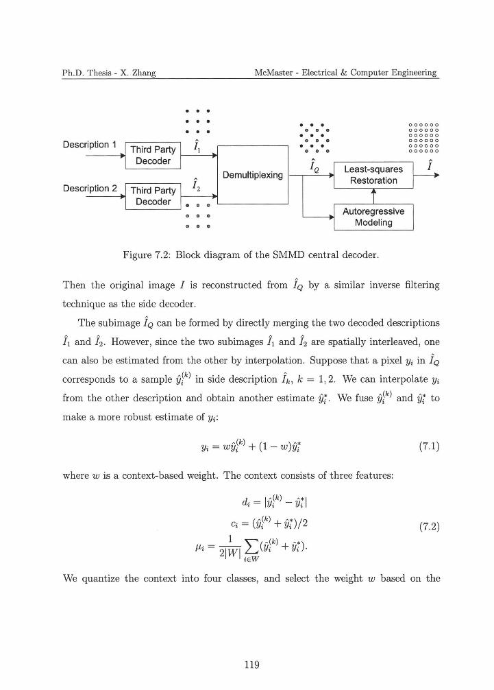
• • • • • •
• • • •
• • •
• •
• • • • • • • • • • • • • • • • • •
Ph.D. Thesis - X. Zhang McMaster - Electrical & Computer Engineering
000000 000000 000000
Third Party JI Decoder
Third Party f2
Decoder • •
Demultiplexing
•
A 000000 000000 000000
Description 1 A
IQ Least-squares Restoration
Description 2
Autoregressive Modeling
Figure 7.2: Block diagram of the SMMD central decoder.
Then the original image I is reconstructed from JQ by a similar inverse filtering
technique as the side decoder.
The subimage JQ can be formed by directly merging the two decoded descriptions
f 1 and f2. However, since the two subimages f1 and f2 are spatially interleaved, one
can also be estimated from the other by interpolation. Suppose that a pixel Yi in JQ corresponds to a sample Y?) in side description ik, k = 1, 2. We can interpolate Yi
from the other description and obtain another estimate Yi. We fuse y;k) and Yi to
make a more robust estimate of yi:
(7.1)
where w is a context-based weight. The context consists of three features:
(7.2)
We quantize the context into four classes, and select the weight w based on the
119
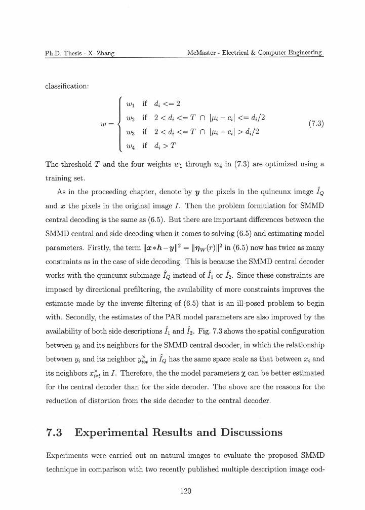
Ph.D. Thesis - X. Zhang McMaster - Electrical & Computer Engineering
classification:
W1 if di<= 2
W2 if 2 <di<= T n lµi - Cil <= di/2 (7.3) w=
W3 if 2 <di<= T n lµi - Cil > di/2
W4 if di> T
The threshold T and the four weights w1 through w4 in (7.3) are optimized using a
training set.
As in the proceeding chapter, denote by y the pixels in the quincunx image fQ
and x the pixels in the original image I. Then the problem formulation for SMMD
central decoding is the same as (6.5). But there are important differences between the
SMMD central and side decoding when it comes to solving (6.5) and estimating model
parameters. Firstly, the term llx*h-yll 2 = ll1Jw(r)ll 2 in (6.5) now has twice as many
constraints as in the case of side decoding. This is because the SMMD central decoder
works with the quincunx subimage fQ instead of f1 or f2 . Since these constraints are
imposed by directional prefiltering, the availability of more constraints improves the
estimate made by the inverse filtering of (6.5) that is an ill-posed problem to begin
with. Secondly, the estimates of the PAR model parameters are also improved by the
availability of both side descriptions i1 and f2. Fig. 7.3 shows the spatial configuration
between Yi and its neighbors for the SMMD central decoder, in which the relationship
between Yi and its neighbor Yi~t in fQ has the same space scale as that between xi and
its neighbors x:Ot in I . Therefore, the the model parameters X can be better estimated
for the central decoder than for the side decoder. The above are the reasons for the
reduction of distortion from the side decoder to the central decoder.
7 .3 Experimental Results and Discussions
Experiments were carried out on natural images to evaluate the proposed SMMD
technique in comparison with two recently published multiple description image cod
120
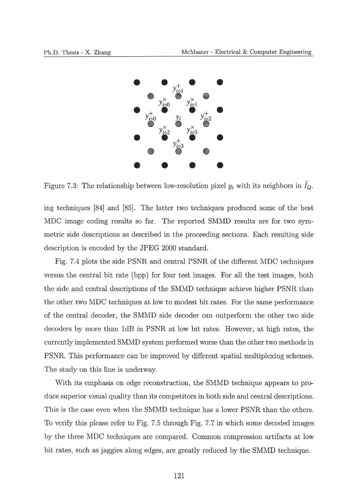
• • • • • • • • • •
Ph.D. Thesis - X. Zhang McMaster - Electrical & Computer Engineering
• • + • •Yiol• x • x •Yi<>O Yiol• + • • + •Yi<>0 Yi Yio2
• +
x• x • •Yio2 Yio3
Yio3
Figure 7.3: The relationship between low-resolution pixel Yi with its neighbors in IQ.
ing techniques [84] and [85]. The latter two techniques produced some of the best
MDC image coding results so far. The reported SMMD results are for two sym
metric side descriptions as described in the proceeding sections. Each resulting side
description is encoded by the JPEG 2000 standard.
Fig. 7.4 plots the side PSNR and central PSNR of the different MDC techniques
versus the central bit rate (bpp) for four test images. For all the test images, both
the side and central descriptions of the SMMD technique achieve higher PSNR than
the other two MDC techniques at low to modest bit rates. For the same performance
of the central decoder, the SMMD side decoder can outperform the other two side
decoders by more than ldB in PSNR at low bit rates. However, at high rates, the
currently implemented SMMD system performed worse than the other two methods in
PSNR. This performance can be improved by different spatial multiplexing schemes.
The study on this line is underway.
With its emphasis on edge reconstruction, the SMMD technique appears to pro
duce superior visual quality than its competitors in both side and central descriptions.
This is the case even when the SMMD technique has a lower PSNR than the others.
To verify this please refer to Fig. 7.5 through Fig. 7.7 in which some decoded images
by the three MDC techniques are compared. Common compression artifacts at low
bit rates, such as jaggies along edges, are greatly reduced by the SMMD technique.
121
Ph.D. Thesis - X. Zhang McMaster - Electrical & Computer Engineering
When losing one description , the SMMD side decoder still preserves edges well
and reconstructs the original image with good visual quality. This can be seen by
comparing Fig. 7.5(e) with Fig. 7.5(f) , and Fig. 7.6(e) with Fig. 7.6(f) . However, a
side description is insufficient to reproduce very high frequency components due to the
spatial downsampling. In this case, the visual quality of the reconstructed image can
be improved significantly by the central decoder when both descriptions are available.
Fig. 7.8 presents three such examples. The high frequency clothes stripes, and the
details such as eyelashes and spokes are reconstructed much better by the central
decoder than the side decoder.
7.4 Conclusion
A spatial multiplexing multiple description scheme for image MDC is proposed in
this chapter. Multiple descriptions are generated by uniformly downsampling in im
age space with adaptive prefiltering. Side decoder reconstructs the input image by
solving an inverse problem with 2D piecewise autoregressive modeling. Central de
coder demultiplexes the multiple descriptions first, and then reconstructs the input
image in a way similar to side decoder, but improves the reconstruction quality with
additional constraints.
122
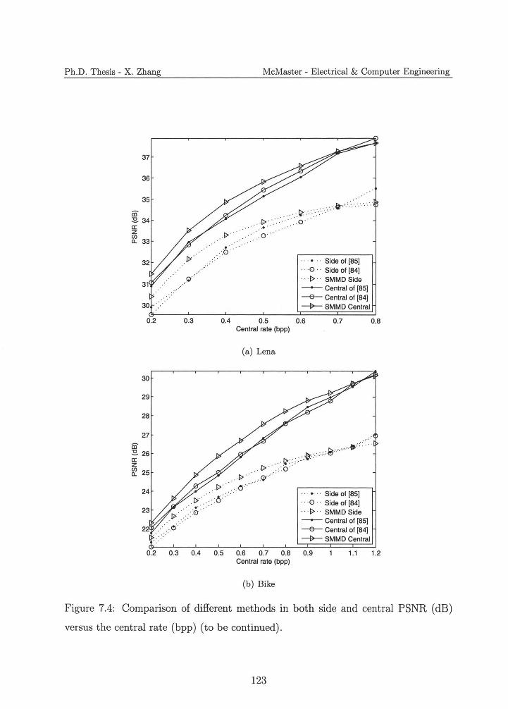
Ph.D. Thesis - X. Zhang McMaster - Electrical & Computer Engineering
37
36
35
co ::!:!. 34 a: z (/) a. 33
.··
.[> . . . .. .. .o ···
··. !;?:·. :·.··_·......... ,·. ~·.'.'.· ....
· · Side of (85] · · ·O · Side of (84] · · ·E> · SMMD Side - Central of (85] --&--- Central of (84]
30 ---ll>-- SMMD Central
0.2 0.3 0.4 0.5 0.6 0.7 0.8 Central rate (bpp)
(a) Lena
30
29
28
27
co ::!:!. 26 a: z ~ 25
24
·:0··
~y···· - ~'·· ··
· · •· · · Side of (85] · · O · · Side of (84] · ·E> · · SMMD Side
- Central of (85] --&--- Central of (84] ---ll>-- SMMD Central
0.2 0.3 0.4 0.5 0.6 0.7 0.8 0.9 1.1 1.2 Central rate (bpp)
(b) Bike
Figure 7.4: Comparison of different methods in both side and central PSNR (dB)
versus the central rate (bpp) (to be continued).
123
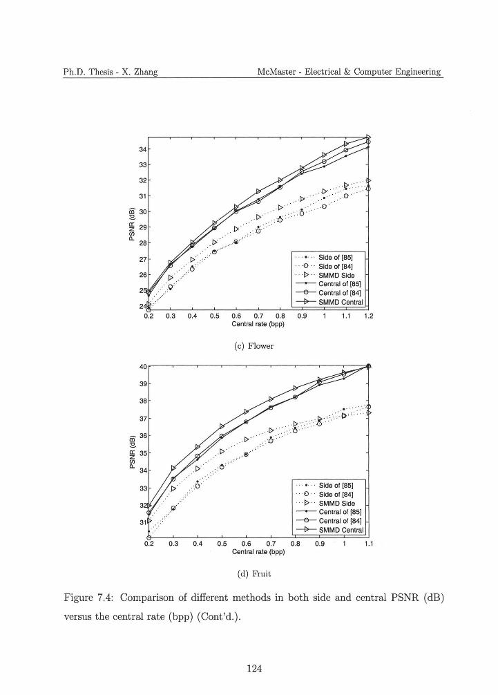
Ph.D. Thesis - X. Zhang McMaster - Electrical & Computer Engineering
34
33
32
31
CD 30 :8. a: 29z (/) Cl.
28
27
2
~ .. ~- ·· :
. . . . . . .
. . [> .o · .• . .. E> ..
E> 6:... ·..I> . :0..
.lil ·· l!J.··
o· ·.. a .
· · Side of [851 · · O · · Side of [84] · · ·E> · · SMMD Side --- Central of [85] ---e- Central of [84]
-+- SMMD Central
2
0.2 0.3 0.4 0.5 0.6 0.7 0.8 0.9 1.1 1.2 Central rate (bpp)
(c) Flower
40
39
38 .•...
37 E> . .. -~ ·· .. [> ''
. [»_·.· ·> 6" . CD 36 .E>. .-0:8. a: 35 , @'. z (/) Cl.
34 .o
.o · · · • · · · Side of [85] .. · · ·O · · Side of [84]
.... · · ·E> · · SMMD Side3 ~ -- Central of [85] ---e- Central of [84]
-+- SMMD Central 31
0.2 0.3 0.4 0.5 0.6 0.7 0.8 0.9 1.1 Central rate (bpp)
(d) Fruit
Figure 7.4: Comparison of different methods in both side and central PSNR (dB)
versus the central rate (bpp) (Cont'd.).
124
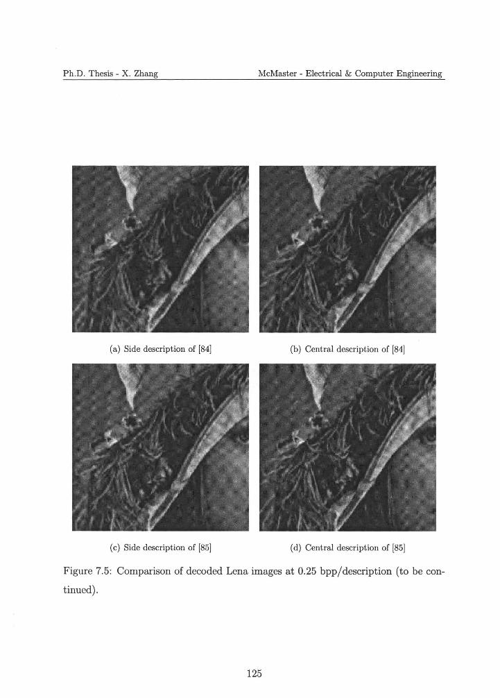
Ph.D. Thesis - X. Zhang McMaster - Electrical & Computer Engineering
(a) Side description of [84] (b) Central description of [84]
(c) Side description of [85] (d) Central description of [85]
Figure 7.5: Comparison of decoded Lena images at 0.25 bpp/description (to be con
tinued).
125
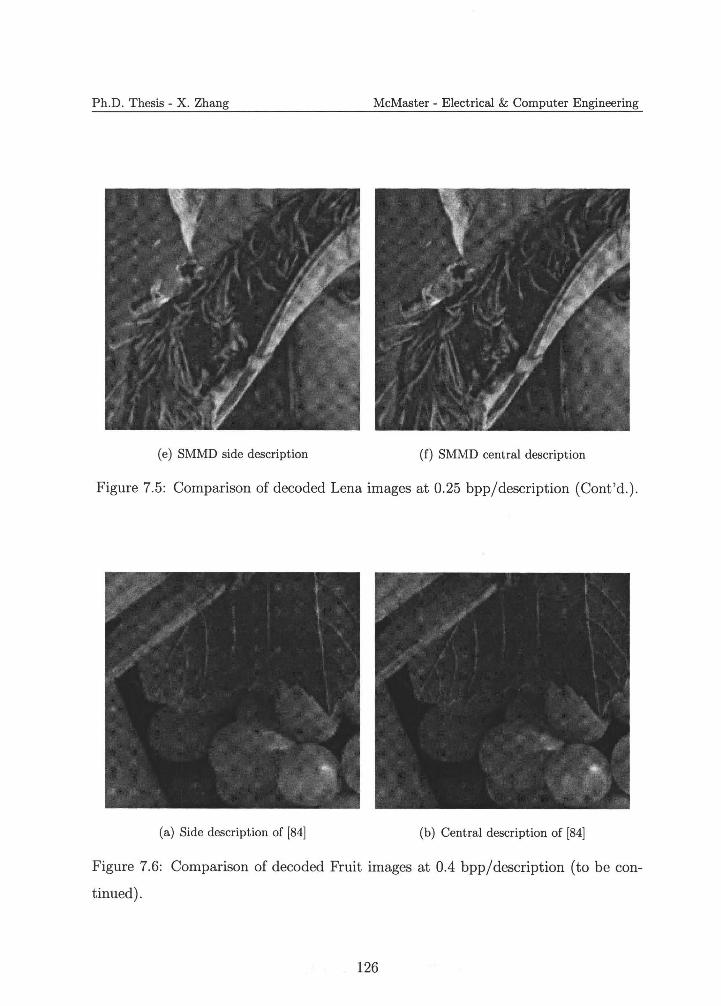
Ph.D. Thesis - X. Zhang McMaster - Electrical & Computer Engineering
(e) SMMD side description (f) SMMD central description
Figure 7.5: Comparison of decoded Lena images at 0.25 bpp/description (Cont'd.).
(a) Side description of [84] (b) Central description of [84]
Figure 7.6: Comparison of decoded Fruit images at 0.4 bpp/description (to be con
tinued).
126
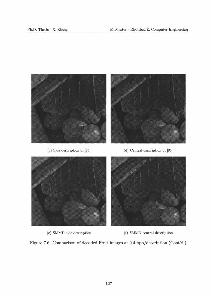
Ph.D. Thesis - X. Zhang McMaster - Electrical & Computer Engineering
(c) Side description of [85] ( d) Central description of [85]
(e) SMMD side description (f) SMMD central description
Figure 7.6: Comparison of decoded Fruit images at 0.4 bpp/description (Cont'd.).
127
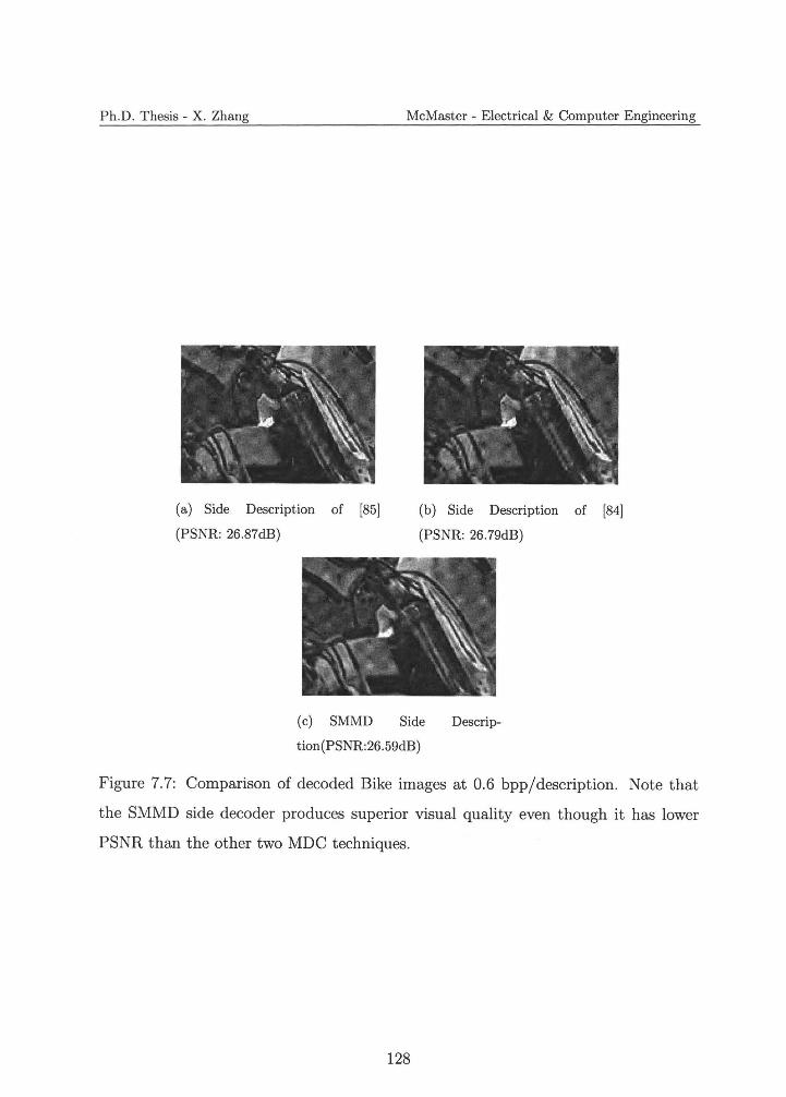
Ph.D. Thesis - X. Zhang McMaster - Electrical & Computer Engineering
(a) Side Description of [85] (b) Side Description of [84]
(PSNR: 26.87dB) (PSNR: 26.79dB)
Side Descrip(c) SMMD
tion(PSNR:26.59dB)
Figure 7.7: Comparison of decoded Bike images at 0.6 bpp/description. Note that
the SMMD side decoder produces superior visual quality even though it has lower
PSNR than the other two MDC techniques.
128
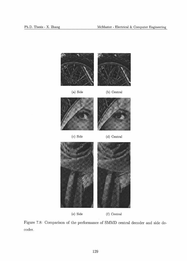
Ph.D. Thesis - X. Zhang McMaster - Electrical & Computer Engineering
(a) Side (b) Central
(c) Side (d) Central
(e) Side (f) Central
Figure 7.8: Comparison of the performance of SMMD central decoder and side de
coder.
129
Ph.D. Thesis - X. Zhang McMaster - Electrical & Computer Engineering
Chapter 8
Conclusions and Future Work
8.1 Conclusions
The research of this thesis advances the state-of-the-art of image interpolation tech
nology and significantly improves the accuracy and visual quality of existing methods.
Three new image interpolation methods are proposed: the first one is a classification
approach that chooses an interpolation direction based on texture orientation; the
second method is a soft-decision approach that estimates missing pixels in blocks
rather than individually to ensure spatial coherence of the reconstructed image; the
third method takes a new model-based nonlinear image restoration approach in which
the model parameters and the unknown HR pixels are jointly estimated. These new
methods have been implemented and thoroughly evaluated in comparison with those
published in the literature. Extensive experiments have been conducted and the re
sults convincingly demonstrate the advantages of the proposed methods over their
predecessors.
In addition, we study and explore the use of image interpolation as a technique
for image compression, in particular for two important scenarios: low bit-rate visual
communication and network-aware multiple description coding. The study results in
two novel standard-compliant interpolation-based compression methods, one for low
130
Ph.D. Thesis - X. Zhang McMaster - Electrical & Computer Engineering
to medium bit rates and the other for multiple descriptions. They generate some
of the best rate-distortion performance reported in the literature in their respective
categories.
Although most of our results are satisfying and among the best so far in the fields,
they can still, we believe, be improved and extended to other topics of image/video
processing. The piecewise autoregressive image model plays a central role in the de
velopment of the SAi and NEARU methods. But the estimation of model parameters
in an LR image is prone to the problem of data overfitting. Currently, we circumvent
the problem by using two separate models of lower order and weighing them. But
a more principled solution should be a unified model whose order is determined in
minimize description length principle. Any progress in this regard will further im
prove the interpolation performance in the future. Another possibility is to choose
from a pool of one-dimensional models of higher order. This may allow us to fully
exploit the anisotropic property of the image signal and interpolate in the direction
of highest statistical redundancy.
Discerning readers may have found our technique of NEARU is a general model
based image restoration framework. With some modifications this framework can be
applied to other image restoration problems, such as video superresolution, denois
ing, deconvolution, deblurring, color demosaicking, and reconstruction of compressive
sensing. This line of research is underway.
131
Bibliography
[1] X. Wu and N. Memon, "Context-based adaptive lossless image coding," IEEE
Transactions on Communications, vol. 45, no. 4, pp. 437- 444, April 1997.
[2] D. Tabuman and M. Marcellin, JPEG2000: Image compression fundamentals ,
standards and parctice. Kluwer Academic Publishers, 2002.
[3] X. Li and M. T. Orchard, "New edge-directed interpolation," IEEE Transactions
on Image Processing, vol. 10, pp. 1521-1527, October 2001.
[4] B. Meyer and P. Tischer, "TMW - a new method for lossless image compression,"
in Proceedings of 1997 Picture Coding Symposium, Berlin, Germany, October
1997.
[5] H. Stark and P. Oskoui , "High-resolution image recovery from image-plane arrays
using convex projections," J. Opt. Soc . Am. A , vol. 6, no. 11, pp. 1715- 1726,
Nov. 1989.
[6] A. V. Oppenheim, A. S. Willsky, and S. H. Nawab, Signals fj Systems, 2nd ed.
Prentice Hall, 1997.
[7] R. G. Keys, "Cubic convolution interpolation for digital image processing," IEEE
Transactions on Acoustic, Speech and Signal Processing, vol. ASSP-29, no. 6, pp.
1153-1160, December 1981.
132
Ph.D. Thesis - X. Zhang McMaster - Electrical & Computer Engineering
[8] X. Zhang and X. Wu, "Image interpolation by adaptive 2-D autoregressive mod
eling and soft-decision estimation," IEEE Transactions on Image Processing,
vol. 17, no. 6, pp. 887-896, June 2008.
[9] X. Wu and X. Zhang, "Image interpolation using texture orientation map and
kernel Fisher discriminant," in Proc. IEEE Int. Conj. Image Processing, vol. 1,
2005, pp. I-49-52.
[10] X. Zhang and X. Wu, "Structure preserving image interpolation via adaptive
2D autoregressive modeling," in Proc. IEEE Int. Conj. Image Processing, vol. 4,
2007, pp. IV- 193 - IV- 196.
[11] X. Wu, X. Zhang, and X. Wang, "Model-based non-linear estimation for adaptive
resolution upconversion and deconvolution," IEEE Trans. on Image Processing,
(under review) .
[12] X. Zhang and X. Wu, "Can lower resolution be better?" in Proc. IEEE Data
Compression Conj., 2008, pp. 302- 311.
[13] X. Wu, X. Zhang, and X. Wang, "Image compression via adaptive down-sampling
and constrained least squares upconversion," IEEE Trans. on Image Processing,
(to appear).
[14] X. Zhang and X. Wu, "Standard-compliant multiple description image coding by
spatial multiplexing and constrained least-squares restoration," in Proc. IEEE
Int. Workshop on Multimedia Signal Processing (MMSP), 2008.
[15] E. Meijering, "A chronology of interpolation: from ancient astronomy to modern
signal and image processing," in Proceedings Of The IEEE, vol. 90, March 2002,
pp. 319-342.
[16] R. C. Gonzalez and R. E. Woods, Digital Image Processing, 2nd ed. Prentice
Hall, 2002.
133
Ph.D. Thesis - X. Zhang McMaster - Electrical & Computer Engineering
[17] S. K. Park and R. A. Schowengerdt, "Image reconstruction by parametric cubic
convolution," Comput. Vis., Graphics, Image Procesing, vol. 23, no. 3, pp. 258
272, 1983.
[18] R. A. Gabel, "Equiripple two-dimensional interpolation filters," in IEEE Int.
Conj. Acoustics, Speech, and Signal Processing (ICASSP), vol. 8, 1983, pp. 387
390.
[19] S. E. Reichenbach and F. Geng, "Two-dimensional cubic convolution," IEEE
Trans. Image Processing, vol. 12, no. 8, pp. 857-865, Aug. 2003.
[20] J. Shi and S. E. Reichenbach, "Image interpolation by two-dimensional para
metric cubic convolution," IEEE Tran. Image Processing, vol. 15, no. 7, pp.
1857-1870, July 2006.
[21] H. S. Hou and H. C. Andrews, "Cubic splines for image interpolation and digital
filtering,'' IEEE Transactions on Acoustic, Speech and Signal Processing, vol. 26,
no. 6, pp. 508-517, December 1978.
[22] E. Maeland, "On the comparison of interpolation methods," IEEE Trans. Med
ical Imaging, vol. 7, pp. 213-217, 1988.
[23] M. Unser, A. Aldroubi, and M. Eden, "Enlargement or reduction of digital images
with minimum loss of information," IEEE Tran. Image Processing, vol. 4, no. 3,
pp. 247-258, Mar. 1995.
[24] M. Unser, "Splines: a perfect fit for signal and image processing," IEEE Signal
Processing Magazine, pp. 22-38, Nov. 1999.
[25] B. Vrcelj and P. P. Vaidyanathan, "Efficient implementation of all-digital inter
polation," IEEE Tran. Image Processing, vol. 10, no. 11, pp. 1639-1646, Nov.
2001.
134
Ph.D. Thesis - X. Zhang McMaster - Electrical & Computer Engineering
[26] C. G. T . M. Lehmann and K. Spizter, "Survey: interpolation methods in medical
image processing," IEEE Transactinos on Medical Imaging, vol. 18, pp. 1049
1075, November 1999.
[27] T. M. Lehmann, C. Gonner, and K. Spitzer, "Addendum: B-spline interpolation
in medical image processing," IEEE Trans. Medical Imaging, vol. 20, no. 7, pp.
660- 665, July 2001.
[28] G. Ramponi, "Warped distance for space-variant linear image interpolation,"
IEEE Trans . Image Processing, vol. 8, no. 5, pp. 629-639, May 1999.
[29] J. Han and S. Baek, "Parametric cubic convolution scaler for enlargement and
reduction of image," IEEE Trans. Consumer Electronics, vol. 46, no. 2, pp. 247
256, May 2000.
[30] H. SHi and R. Ward, "Canny edge based image expansion," in IEEE Int. Sym
posium on Circuits and Systems, vol. 1, 2002, pp. 1- 785 - 1-788.
[31] J . W. Hwang and H. S. Lee, "Adaptive image interpolation based on local gradi
ent features," IEEE Signal Processing Letters, vol. 11, no. 3, pp. 359- 362, March
2004.
[32] C. Vazquez, E. Dubois, and J. Konrad, "Reconstruction of nonuniformly sampled
images in spline spaces," IEEE Trans. Image Processing, vol. 14, no. 6, pp. 713
725, June 2005.
[33] K. Jensen and D. Anastassiou, "Subpixel edge localization and the interpolation
of still images,'' IEEE Transactions on Image Processing, vol. 4, pp. 285-295,
March 1995.
[34] J. Allebach and P. W. Wong, "Edge-directed interpolation," in Proc. IEEE Int.
Conj. Image Processing, vol. 3, 1996, pp. 707-710.
135
Ph.D. Thesis - X. Zhang McMaster - Electrical & Computer Engineering
[35] S. Dube and L. Hong, "An adaptive algorithm for image resolution enhance
ment," in Singals, Systems and Computers, vol. 2, 2000, pp. 1731-1734.
[36] S. Carrato and L. Tenze, "A high quality 2x image interpolator," IEEE Signal
Processing Letters, vol. 7, pp. 132-135, June 2000.
[37] F. Malgouyres and F. Guichard, "Edge direction preserving image zooming: a
mathematical and numerical analysis," SIAM J. Numer. Anal., vol. 39, pp. 1-37,
2001.
[38] Q. Wang and R. Ward, "A new edge-directed image expansion scheme," in IEEE
Int. Conj. Image Processing (ICIP), vol. 3, 2001, pp. 899- 902.
[39] D. D. Muresan, "Fast edge directed polynomial interpolation," IEEE Int. Conj.
Image Processing (!GIP) , vol. 2, pp. II-990-3, Nov. 2005.
[40] Q. Wang and R. K. Ward, "A new orientation-adaptive interpolation method,"
IEEE Trans. Image Processing, vol. 16, no. 4, pp. 889-900, Apr. 2007.
[41] D. D. Muresan and T . W. Parks, "Adaptively quadratic (AQua) image inter
polation," IEEE Transactions on Image Processing, vol. 13, no. 5, pp. 690-698,
May 2004.
[42] L. Zhang and X. Wu, "Image interpolation via directional filtering and data
fusion," IEEE Transactions on Image Processing, vol. 15, no. 8, pp. 2226- 2238,
August 2006.
[43] Y. Cha and S. Kim, "Edge-forming methods for image zooming," Journal of
Mathematical Imaging and Vision, vol. 25, no. 3, pp. 353-364, Oct. 2006.
[44] --, "Edge-forming methods for color image zooming," IEEE Trans. Image
Processing, vol. 15, no. 8, pp. 2315-2323, Aug. 2006.
136
Ph.D. Thesis - X. Zhang McMaster - Electrical & Computer Engineering
[45] M. Li and T. Q. Nguyen, "Markov random field model-based edge-directed image
interpolation," IEEE Trans. Image Processing, vol. 17, no. 7, pp. 1121-1128, July
2008.
[46] W. K. Carey, D. B. Chuang, and S. S. Hemami, "Regularity-preserving image
interpolation," IEEE Transactions on Image Processing, vol. 8, no. 9, pp. 1293
1297, September 1999.
[47] Y. Zhu, S. C. Schwartz, and M. T. Orchard, "Wavelet domain image interpolation
via statistical estimation," in Proceedings of International Conference on Image
Processing, vol. 3, September 2001, pp. 840-843.
[48] D. D. Muresan and T . W. Parks, "Prediction of image detail,'' in Proceedings
of International Conference on Image Processing, vol. 2, September 2000, pp.
323-326.
[49] S. G. Chang and Z. Cvetkovic, "Locally adaptive wavelet-based image inter
polation," IEEE Trans. Image Processing, vol. 15, no. 6, pp. 1471-1485, June
2006.
[50] A. Temizel and T. Vlachos, "Wavelet domain image resolution enhancement,''
IEE Proc. Vis . Image Signal Processing, vol. 153, no. 1, pp. 25-30, Feb. 2006.
[51] A. Tsai, A. Y. Jr., and A. S. Willsky, "Curve evolution implementation of the
Mumford-Shah functional for image segmentation, denoising, interpolation, and
magnification,'' IEEE Trans. Image Processing, vol. 10, no. 8, pp. 1169-1186,
Aug. 2001.
[52] W. T. Freeman, T. R. Jones, and E. C. Pasztor, "Example-based superresolu
tion,'' IEEE Comput. Graphics Appl., vol. 22, no. 2, pp. 56-65, Mar. 2002.
137
Ph.D. Thesis - X. Zhang McMaster - Electrical & Computer Engineering
[53] S. Baker and T. Kanade, "Limits on super-resolution and how to break them,"
IEEE Trans. Patttern Analysis and Machine Intelligence, vol. 24, no. 9, pp.
1167- 1183, Sept. 2002.
[54] J . Sun, N. Zheng, and H. S. H. Tao, "Image hallucination with primal sketch pri
ors," in IEEE Proceedings on Computer Vision and Pattern Recognition, vol. 2,
June 2003, pp. 11- 7 29-36.
[55] C. Lin, K. Fan, H. Pu, S. Lu, and S. Liang, "An RVS-directed neural-network
based image resolution enhancement scheme for image resizing," IEEE Trans.
Fuzzy Systems, vol. 15, no. 4, pp. 605- 615, Aug. 2007.
[56] R. R. Schultz and R. L. Stevenson, "A bayesian approach to image expansion for
improved definition," IEEE Trans . Image Processing, vol. 3, no. 3, pp. 233-242,
May 1994.
[57] K. Ratakonda and N. Ahuja, "POCS based adaptive image manification," m
Proc. IEEE Int. Conj. Image Processing, vol. 3, 1998, pp. 203- 207.
[58] D. Calle and A. Montanvert , "Superresolution inducing of an image," in Proc.
IEEE Int. Conj. Image Processing, vol. 3, 1998, pp. 232- 235.
[59] F . Fekri , R. M. Mersereau, and R. W. Schafer, "A generalized interpolative
vector quantization method for jointly optimal quantization, interpolation, and
binarization of text images," IEEE Trans. Image Processing, vol. 9, no. 7, pp.
1272- 1281, July 2000.
[60] N. A. Woods, N. P. Galatsanos, and A. K. Katsaggelos, "Stochastic methods
for joint registration , restoration, and interpolation of multiple undersampled
images," IEEE Trans. Image Processing, vol. 15, no. 1, pp. 201-213, Jan. 2006.
138
Ph.D. Thesis - X. Zhang McMaster - Electrical & Computer Engineering
[61] H. Takeda, S. Farsiu, and P. Milanfer, "Kernel regression for image processing
and reconstruction," IEEE Trans. Image Processing, vol. 16, no. 2, pp. 349-366,
Feb. 2007.
[62] J. Kopf, M. Cohen, D. Lischinski, and M. Uyttendaele, "Joint bilateral upsam
pling," ACM Transactions on Graphics {Proceedings of SIGGRAPH), vol. 26,
no. 3, pp. 96-1 - 96-6, July 2007.
[63] B. Zeng and A. N. Venetsanopoulos, "A JPEG-based interpolative image coding
scheme," in Proc. IEEE ICASSP, vol. 5, 1993, pp. 393-396.
[64] A. M. Bruckstein, M. Elad, and R. Kimmel, "Down-scaling for better transform
compression," IEEE Trans. Image Processing, vol. 12, no. 9, pp. 1132-1144, Sept.
2003.
[65] A. S. A, M. E. B, P. M. C, R. W. A, and C. F. A, "Improved high-definition
video by encoding at an intermediate resolution," in Proc. SPIE Visual Commu
nications and Image Processing, vol. 5308, 2004, pp. 1007-1018.
[66] Y. Tsaig, M. Elad, and P. Milanfar, "Variable projection for near-optimal filtering
in low bit-rate block coders," IEEE Trans. Circuits Syst. Video Technol., vol. 15,
no. 1, pp. 154-160, Jan. 2005.
[67] W. Lin and D. Li, "Adaptive downsampling to improve image compression at
low bit rates," IEEE Trans. Image Processing, vol. 15, no. 9, pp. 2513-2521,
Sept. 2006.
[68] L. Gan, C. Tu, J. Liang, T. D. Tran, and K.-K. Ma, "Undersampled boundary
pre-/post-filters for low bit-rate <let-based coders," IEEE Trans. Image Process
ing, vol. 16, no. 2, pp. 428-441, Feb. 2007.
[69] A. K. Jain and F. Farrokhnia, "Unsupervised texture segmentation using Gabor
filters," Pattern Recognition, vol. 24, no. 12, pp. 1167-1186, 1991.
139
Ph.D. Thesis - X. Zhang McMaster - Electrical & Computer Engineering
[70] M. Xu, X. Wu, and P. Franti, "Context quantization by kernel Fisher discrimi
nant,'' IEEE Tran. Image Processing, vol. 15, no. 1, pp. 169- 177, January 2006.
[71] S. Mika, G. Ratsch, J. Weston, B. Scholkopf, A. J. Smola, , and K. R. Muller ,
"Invariant feature extraction and classification in kernel spaces,'' in Advances in
neural information processing systems, vol. 12. MIT Press, 2000, pp. 526-532.
[72] X. Wu, K. U. Barthel, and W. Zhang, "Piecewise 2D autoregression for predictive
image coding." in Proceedings of the IEEE Int. Conj. on Image Processing, vol. 3,
Chicago, Oct. 1998, pp. 901-904.
[73] A. Said and W. Pearlman, "An image multiresolution representation for lossless
and lossy compression," IEEE Trans. Image Processing, vol. 5, pp. 1303- 1330,
September 1996.
[74] I. Matsuda, H. Mori , J. Maeda, and S. Itoh, "Design and evaluation of minimum
rate predictors for lossless image coding,'' Trans. IEICE (DI!) , vol. J85-D-II ,
no. 3, pp. 448- 456, March 2002, (in Japanese) .
[75] J . More, "The Levenberg-Marquardt algorithm: implementation and theory,"
Numerical Analysis, pp. 105-116, 1977.
[76] G. Golub and V. Pereyra, "Separable nonlinear least squares: the variable pro
jection method and its applications,'' Inverse Problems, vol. 19, no. 2, pp. 1- 26,
Feb. 2003.
[77] J. Rosen, H. Park, and J . Glick, "Structured total least norm for nonlinear
problem,'' SIAM J. Matrix Anal. Appl., vol. 20, no. 1, pp. 14- 30, Jan. 1998.
[78] E. Cands, "Compressive sampling,'' in Proceedings of the Int. Congress of Math
ematics, Madrid, Spain, 2006, pp. 1433- 1452.
140
Ph.D. Thesis - X. Zhang McMaster - Electrical & Computer Engineering
[79] X. Li and M. T . Orchard, "Edge-direted prediction for lossless compression of
natural images," IEEE Transactions on Image Processing, vol. 10, no. 6, pp.
813- 817, June 2001.
[80] D. Santa-Cruz., R. Grosbois, and T . Ebrahimi, "JPEG 2000 performance evalu
ation and assessment," Signal Processing: Image Communication, vol. 1, no. 17,
pp. 113-130, 2002.
[81] X. Zhang, X. Wu, and F. Wu, "Image coding on quincunx lattice with adaptive
lifting and interpolation," in IEEE Data Compression Conference 2007, Mar.
2007, pp. 193-202.
[82] S. D. Servetto, K. Ramchandran, V. Vaishampayan, and K. Nahrstedt, "Multiple
description wavelet based image coding," IEEE Trans. Image Processing, vol. 9,
no. 5, pp. 813-826, May 2000.
[83] C. Tian and S. S. Hemami, "A new class of multiple description scalar quantizer
and its application to image coding," IEEE Signal Processing Letter, vol. 12,
no. 4, pp. 329-332, Mar. 2007.
[84] J. Wang and J. Liang, "Filter banks for prediction-compensated multiple de
scription coding," in IEEE Data Compression Conj, 2008, pp. 392-401.
[85] T. Tillo, M. Grangetto, and G. Olmo, "Multiple description image coding based
on Lagrangian rate allocation," IEEE Trans. Image Processing, vol. 16, no. 3,
pp. 673-683, March 2007.
141


