Embed Size (px)
Citation preview
59
Chapter 3. Interpolation and Curve Fitting
Relevant Computer Lab Exercises are attached to the end of this Chapter, p. 73 and p. 75
Many problems in engineering require mathematical functions to be fitted to discrete data. These data
typically correspond to experimental measurements or field observations, and the fitting functions used
are, usually (but not always) polynomials. Once the mathematical function has been derived, it is
possible to interpolate between the known discrete values in a consistent and reliable way.
Broadly speaking, there are two different strategies for deriving approximation functions. The first
approach, which is generally described as the interpolation method, chooses the function so that it
matches the discrete data exactly at every point. The second approach, which is often loosely described
as curve fitting, chooses the function merely to provide a "good fit" to the discrete data but does not
necessarily pass through all of the points. Both of these techniques will be discussed in this Chapter.
An nth degree polynomial is defined by an expansion of the form
n
nn xaxaxaaxp 2
210)( (3.1)
where a0, a1, .., an are constants, some of which may be zero. Examples of polynomials are
P 1 (x) = 2 + 3x (linear - first order)
P 1 (x) = 3x (linear - first order)
P2(x) = 4.2 + 3x + 2.75x2 (quadratic - second order)
P3(x) = 2.75x2 + x
3 (cubic - third order)
Note that it is the highest power of x that determines the order of the polynomial.
3.1 Taylor Polynomial Interpolation
Taylor interpolation is used where a polynomial approximation to a known mathematical function is
needed near a specified point. The method does not attempt to approximate a function over an interval
and should not be used for this purpose.
To illustrate the steps in the Taylor method, consider a third degree polynomial approximation
P3(x) = a0 + a1x + a2x2 + a3x
3 (3.2)
to the function f(x) = sin(x) in the vicinity of x0 = 0. The four constants a0, a1, a2, a3 are chosen so that
p3(x) matches f(x), and as many of its derivatives as possible, at the specified point. By inspection, we
can match the function and its first, second and third derivatives at the point x = 0 by imposing the
conditions
p3(0) = f (0) = sin(0) = 0
p3' (0) = f ' (0) = cos(0) = 1
P3" (0) = f " (0) = – sin(0) = 0
p3"' (0) = f "' (0) = – cos(0)= – 1
Now from (3.2) we see that
p3(0) = a0
p3' (0) = a1
P3" (0) =2 a2
p3"' (0) = 6 a3
and hence
a0 = 0 (3.3)
a1 = 1 (3.4)
2 a2 = 0 (3.5)
60
6 a3 = –1 (3.6)
Substituting in (3.2) gives the Taylor polynomial as
3
36
1)( xxxp (3.7)
Thus, in the vicinity of x = 0, we can write that
3
6
1)sin( xxx (3.8)
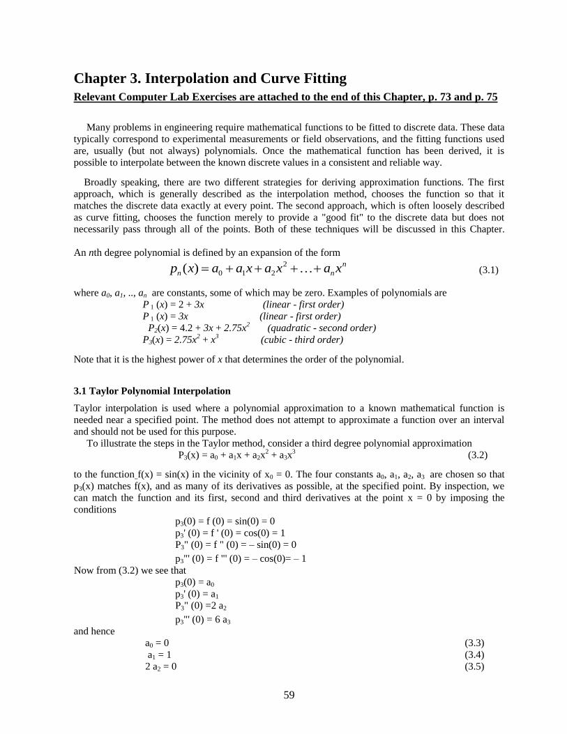
For example, at x = 0.2 radians, the Taylor approximation gives sin(x) 0.198667. This compares well
with the exact value of sin (x) = 0.198669. A plot of the third degree Taylor polynomial, shown in Figure
3.1, indicates that it gives reasonably good approximations provided |x| 1.5 radians. For values of x
outside this range, the approximation rapidly becomes inaccurate.
Figure 3.1 Taylor polynomial approximation to sin(x) near x = 0.
3.2 Lagrange Interpolation
Lagrange interpolation provides a method for defining a polynomial which approximates a function over
an interval. The polynomial is defined uniquely by insisting that it matches the function exactly at a
specified number of points. The general form of the Lagrange polynomial is
Pn(x) = l0 (x) f (x0) + l1 (x) f (x1) + … + ln (x) f (xn) (3.9)
where f (x0), f (x1), …, f (xn) are known and l0 (x), l1 (x), …, ln (x) are Lagrange interpolation
functions. An exact fit is obtained at each of the n + 1 points by insisting that
Pn(x0) = f (x0)
Pn(x1) = f (x1) (3.10)
x
f(x)
p3(x)
-3 -2 -1 3 2 1 0 -3
-2
-1
3
2
1
0
61
Pn(xn) = f (xn)
For a set of n+ 1 data points, the Lagrange interpolation functions have degree n and are defined by
n
ijj ji
j
niiiiiii
nii
i
xx
xx
xxxxxxxxxx
xxxxxxxxxxxl
0
1100
1100
)(
)(
)())(())((
)())(())(()(
(3.11)
for i = 0, 1, …, n. The Lagrange interpolation functions li (x) vanish at xj for all j i and take the value 1
at xi. This property may be stated mathematically as
ji
jixl ji
,0
,1)( (3.12)
for i, j = 0, 1, …, n and guarantees that the conditions of (3.10) are satisfied precisely.
To illustrate the use of Lagrange interpolation, consider the linear approximation of the function f(x) =
x2 over the interval [1,2] using the points x0 = 1 and x1 = 2. Using (3.11), we obtain the linear Lagrange
interpolation functions as
10
10 )(
xx
xxxl
01
01 )(
xx
xxxl
Note that
1)(10
1000
xx
xxxl 1)(
01
0111
xx
xxxl
0)(10
1110
xx
xxxl 0)(
01
0001
xx
xxxl
so that the conditions of (3.12) are satisfied. The linear form of (3.9) gives the Lagrange polynomial as
)()()( 1
01
00
10
11 xf
xx
xxxf
xx
xxxp
(3.13)
Substituting the known values
x0 = 1 f(x0) = 1
x1 = 2 f(x1) = 4
into (3.13) we obtain
23412
11
21
2)(1
x
xxxp (3.14)
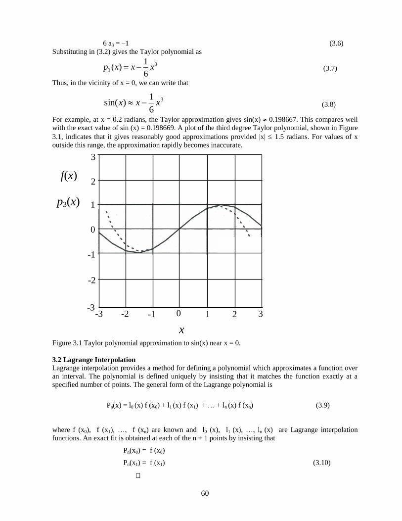
This Lagrange polynomial, shown in Figure 3.2, is simply the equation
62
Figure 3.2: Linear Lagrange interpolation
of the line that connects the two end points. As a check on (3.l4), we note that
)(1213)1()( 001 xfpxp
)(4223)2()( 111 xfpxp
so that the p1(x) matches f(x) precisely at the data points. It is also important to note that Lagrange
interpolation should not be used outside the interval over which the approximation is defined, since
the results are usually very inaccurate. In practice, the number of points required to approximate the
function accurately over an interval must be determined by trial and error.
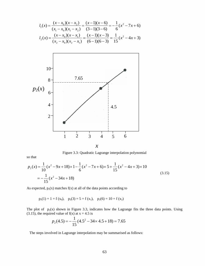
To illustrate the use of Lagrange interpolation for a more complex example, consider the data points
point x f(x)
0 1 1
1 3 5
2 6 10
and estimate the value of f(x) at x = 4.5. Since there are three data points, a second order Lagrange
polynomial of the form:
p2(x) = l0 (x) f (x0) + l1 (x) f (x1) + l2 (x) f (x2)
is appropriate. Using (3.11) we obtain
)189(10
1
)61)(31(
)6)(3(
))((
))(()( 2
2010
210
xx
xx
xxxx
xxxxxl
3
x
1.0 2.0
1
4
2
5
p1(x) = 3x - 2
f(x) = x2
f(x)
f(x1)
f(x0)
x1 x0
63
)67(6
1
)63)(13(
)6)(1(
))((
))(()( 2
2101
201
xx
xx
xxxx
xxxxxl
)34(15
1
)36)(16(
)3)(1(
))((
))(()( 2
1202
102
xx
xx
xxxx
xxxxxl
Figure 3.3: Quadratic Lagrange interpolation polynomial
so that
)1834(15
1
10)34(15
15)67(
6
11)189(
10
1)(
2
222
2
xx
xxxxxxxp
(3.15)
As expected, p2(x) matches f(x) at all of the data points according to
p2(1) = 1 = f (x0), p2(3) = 5 = f (x1), p2(6) = 10 = f (x2)
The plot of p2(x) shown in Figure 3.3, indicates how the Lagrange fits the three data points. Using
(3.15), the required value of f(x) at x = 4.5 is
65.7)185.4345.4(15
1)5.4( 2
2 p
The steps involved in Lagrange interpolation may be summarised as follows:
x
p2(x)
1 2 3 4 6 5
2
4
6
8
10
7.65
4.5
64
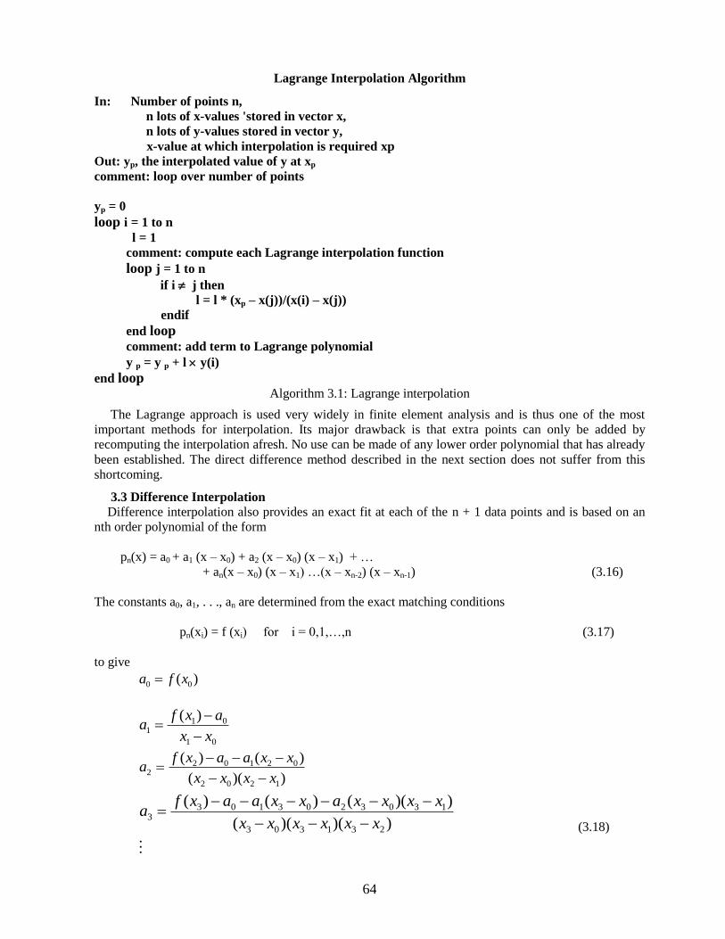
Lagrange Interpolation Algorithm
In: Number of points n,
n lots of x-values 'stored in vector x,
n lots of y-values stored in vector y,
x-value at which interpolation is required xp
Out: yp, the interpolated value of y at xp
comment: loop over number of points
yp = 0
loop i = 1 to n
l = 1
comment: compute each Lagrange interpolation function
loop j = 1 to n
if i j then
l = l * (xp – x(j))/(x(i) – x(j))
endif
end loop
comment: add term to Lagrange polynomial
y p = y p + l y(i)
end loop
Algorithm 3.1: Lagrange interpolation
The Lagrange approach is used very widely in finite element analysis and is thus one of the most
important methods for interpolation. Its major drawback is that extra points can only be added by
recomputing the interpolation afresh. No use can be made of any lower order polynomial that has already
been established. The direct difference method described in the next section does not suffer from this
shortcoming.
3.3 Difference Interpolation Difference interpolation also provides an exact fit at each of the n + 1 data points and is based on an
nth order polynomial of the form
pn(x) = a0 + a1 (x – x0) + a2 (x – x0) (x – x1) + …
+ an(x – x0) (x – x1) …(x – xn-2) (x – xn-1) (3.16)
The constants a0, a1, . . ., an are determined from the exact matching conditions
pn(xi) = f (xi) for i = 0,1,…,n (3.17)
to give
)( 00 xfa
01
011
)(
xx
axfa
))((
)()(
1202
021022
xxxx
xxaaxfa
))()((
))(()()(
231303
13032031033
xxxxxx
xxxxaxxaaxfa
(3.18)
65
As mentioned previously, extra data points can be included in the difference interpolation merely by
adding extra terms to an existing polynomial. This means that, unlike the Lagrangian approach, the
interpolation does not have to be recomputed from scratch.
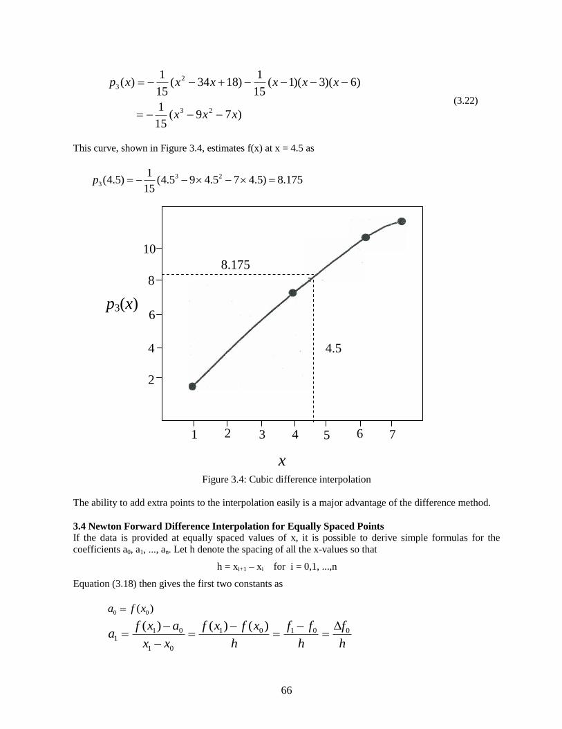
To illustrate the use of difference interpolation, consider the data points
point X f(x)
0 1 1
1 3 5
2 6 10
3 5 9
and estimate f(x) at x = 4.5. Since there are four points, the final order of p(x) will be cubic. Before
computing this cubic polynomial, however, we will derive the quadratic difference polynomial for the
first three points and then modify this subsequently to incorporate the fourth point. Note that the first
three data points are identical to those used for Lagrangian interpolation. Because the quadratic
polynomial passing through any three points in the plane is unique, we would expect the interpolating
polynomial to be the same. Applying (3.18) to the first three points furnishes
1)( 00 xfa
223
15)(
01
011
xx
axfa
15
1
)26)(16(
)16(2110
))((
)()(
1202
021022
xxxx
xxaaxfa
so that (3.16) becomes
)1834(15
1
)3)(1(15
1)1(21)(
2
2
xx
xxxxp
(3.19)
As predicted, this is identical to the polynomial obtained from Lagrangian interpolation. Addition of the
fourth point (5,9) to the interpolation gives the extra constant
15
1
)65)(35)(15(
)35)(15(15/1)15(219
))()((
))(()()(
231303
13032031033
xxxxxx
xxxxaxxaaxfa
(3.20)
(3.21)
Equation (3.16) then furnishes the cubic interpolating polynomial as
66
)79(15
1
)6)(3)(1(15
1)1834(
15
1)(
23
2
3
xxx
xxxxxxp
(3.22)
This curve, shown in Figure 3.4, estimates f(x) at x = 4.5 as
175.8)5.475.495.4(15
1)5.4( 23
3 p
Figure 3.4: Cubic difference interpolation
The ability to add extra points to the interpolation easily is a major advantage of the difference method.
3.4 Newton Forward Difference Interpolation for Equally Spaced Points
If the data is provided at equally spaced values of x, it is possible to derive simple formulas for the
coefficients a0, a1, ..., an. Let h denote the spacing of all the x-values so that
h = xi+1 – xi for i = 0,1, ...,n
Equation (3.18) then gives the first two constants as
)( 00 xfa
h
f
h
ff
h
xfxf
xx
axfa 00101
01
011
)()()(
x
p3(x)
1 2 3 4 6 5
2
4
6
8
10
8.175
4.5
7
67
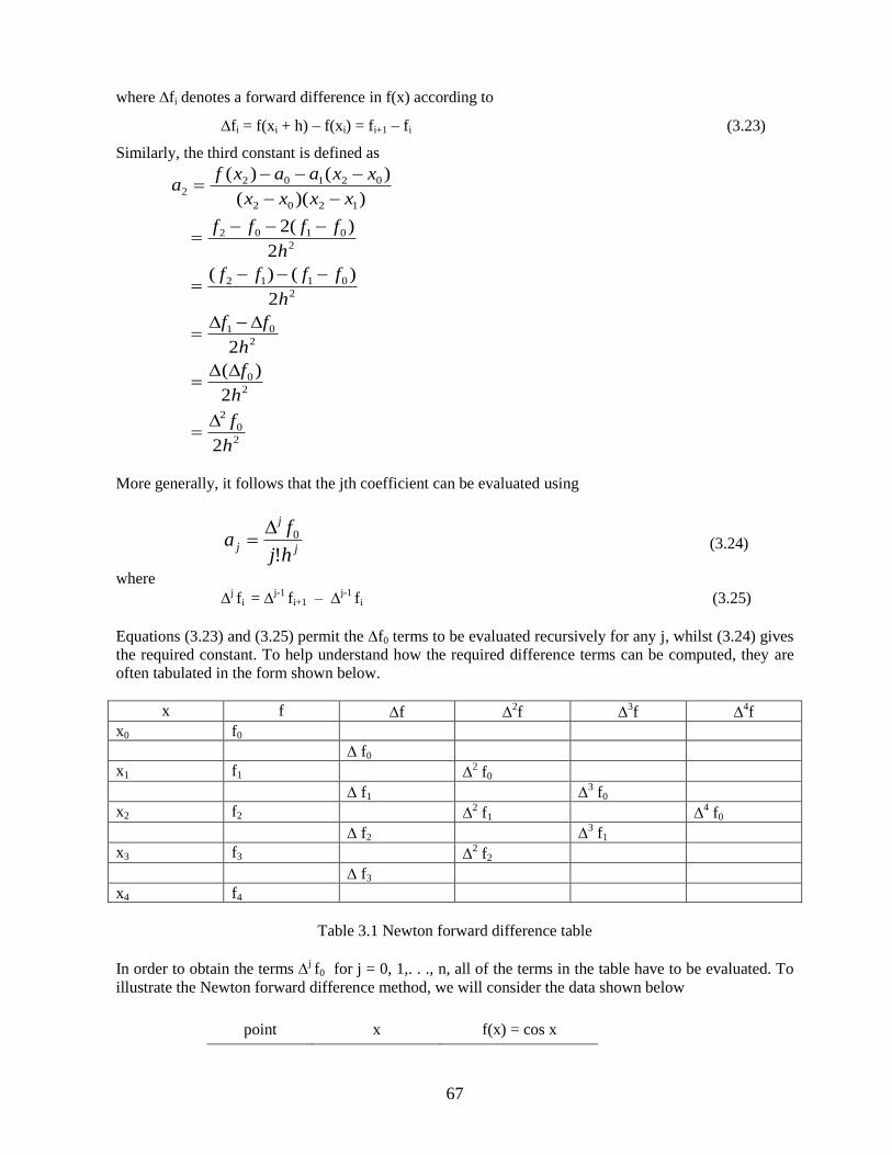
where fi denotes a forward difference in f(x) according to
fi = f(xi + h) – f(xi) = fi+1 – fi (3.23)
Similarly, the third constant is defined as
2
0
2
2
0
2
01
2
0112
2
0102
1202
021022
2
2
)(
2
2
)()(
2
)(2
))((
)()(
h
f
h
f
h
ff
h
ffff
h
ffff
xxxx
xxaaxfa
More generally, it follows that the jth coefficient can be evaluated using
j
j
jhj
fa
!
0 (3.24)
where
j fi =
j-1 fi+1 –
j-1 fi (3.25)
Equations (3.23) and (3.25) permit the f0 terms to be evaluated recursively for any j, whilst (3.24) gives
the required constant. To help understand how the required difference terms can be computed, they are
often tabulated in the form shown below.
x f f 2f
3f
4f
x0 f0
f0
x1 f1 2 f0
f1 3 f0
x2 f2 2 f1
4 f0
f2 3 f1
x3 f3 2 f2
f3
x4 f4
Table 3.1 Newton forward difference table
In order to obtain the terms j f0 for j = 0, 1,. . ., n, all of the terms in the table have to be evaluated. To
illustrate the Newton forward difference method, we will consider the data shown below
point x f(x) = cos x
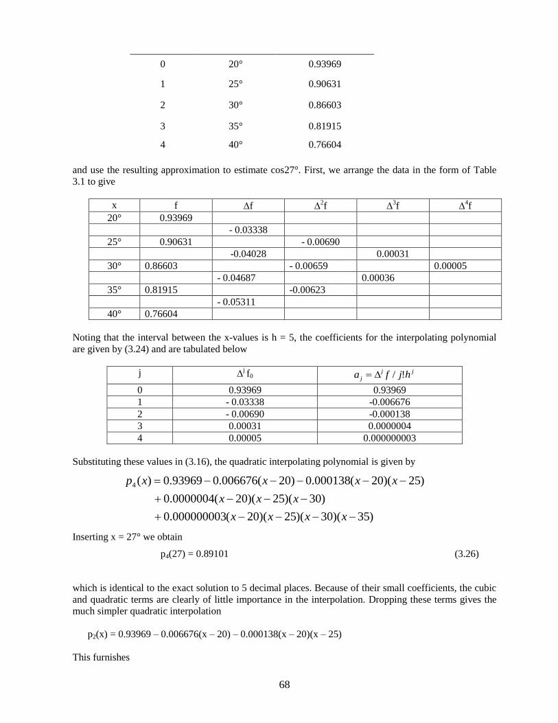
68
0 20° 0.93969
1 25° 0.90631
2 30° 0.86603
3 35° 0.81915
4 40° 0.76604
and use the resulting approximation to estimate cos27°. First, we arrange the data in the form of Table
3.1 to give
x f f 2f
3f
4f
20° 0.93969
- 0.03338
25° 0.90631 - 0.00690
-0.04028 0.00031
30° 0.86603 - 0.00659 0.00005
- 0.04687 0.00036
35° 0.81915 -0.00623
- 0.05311
40° 0.76604
Noting that the interval between the x-values is h = 5, the coefficients for the interpolating polynomial
are given by (3.24) and are tabulated below
j j f0
jj
j hjfa !/
0 0.93969 0.93969
1 - 0.03338 -0.006676
2 - 0.00690 -0.000138
3 0.00031 0.0000004
4 0.00005 0.000000003
Substituting these values in (3.16), the quadratic interpolating polynomial is given by
)35)(30)(25)(20(000000003.0
)30)(25)(20(0000004.0
)25)(20(000138.0)20(006676.093969.0)(4
xxxx
xxx
xxxxp
Inserting x = 27° we obtain
p4(27) = 0.89101 (3.26)
which is identical to the exact solution to 5 decimal places. Because of their small coefficients, the cubic
and quadratic terms are clearly of little importance in the interpolation. Dropping these terms gives the
much simpler quadratic interpolation
p2(x) = 0.93969 – 0.006676(x – 20) – 0.000138(x – 20)(x – 25)
This furnishes
69
p2(27) = 0.89103 (3.27)
which is accurate to four decimal places.
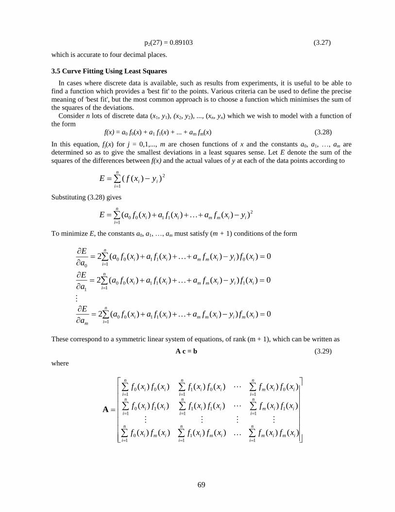
3.5 Curve Fitting Using Least Squares
In cases where discrete data is available, such as results from experiments, it is useful to be able to
find a function which provides a 'best fit' to the points. Various criteria can be used to define the precise
meaning of 'best fit', but the most common approach is to choose a function which minimises the sum of
the squares of the deviations.
Consider n lots of discrete data (x1, y1), (x2, y2), ..., (xn, yn) which we wish to model with a function of
the form
f(x) = a0 f0(x) + a1 f1(x) + ... + am fm(x) (3.28)
In this equation, fj(x) for j = 0,1,..., m are chosen functions of x and the constants a0, a1, …, am are
determined so as to give the smallest deviations in a least squares sense. Let E denote the sum of the
squares of the differences between f(x) and the actual values of y at each of the data points according to
n
iii yxfE
1
2))((
Substituting (3.28) gives
n
iiimmii yxfaxfaxfaE
1
2
1100 ))()()((
To minimize E, the constants a0, a1, …, am must satisfy (m + 1) conditions of the form
0)())()()((2 01
1100
0
i
n
iiimmii xfyxfaxfaxfa
a
E
0)())()()((2 11
1100
1
i
n
iiimmii xfyxfaxfaxfa
a
E
0)())()()((21
1100
im
n
iiimmii
m
xfyxfaxfaxfaa
E
These correspond to a symmetric linear system of equations, of rank (m + 1), which can be written as
A c = b (3.29)
where
n
iimim
n
iimi
n
iimi
n
iiim
n
iii
n
iii
n
iiim
n
iii
n
iii
xfxfxfxfxfxf
xfxfxfxfxfxf
xfxfxfxfxfxf
111
10
11
111
110
10
101
100
)()()()()()(
)()()()()()(
)()()()()()(
A
70
n
iiim
n
iii
n
iii
yxf
yxf
yxf
1
11
10
)(
)(
)(
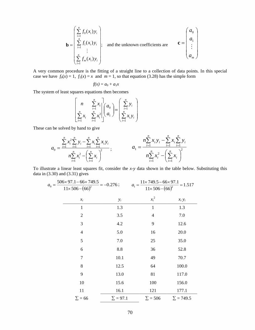
b ; and the unknown coefficients are
ma
a
a
1
0
c
A very common procedure is the fitting of a straight line to a collection of data points. In this special
case we have f0(x) = 1, f1(x) = x and m = 1, so that equation (3.28) has the simple form
f(x) = a0 + a1x
The system of least squares equations then becomes
n
iii
n
ii
n
ii
n
ii
n
ii
yx
y
a
a
xx
xn
1
1
1
0
1
2
1
1
These can be solved by hand to give
2
11
2
1 111
2
0
n
ii
n
ii
n
i
n
iii
n
iii
n
ii
xxn
yxxyx
a ; 2
11
2
1 111
n
ii
n
ii
n
i
n
ii
n
iiii
xxn
yxyxn
a
To illustrate a linear least squares fit, consider the x-y data shown in the table below. Substituting this
data in (3.30) and (3.31) gives
276.06650611
5.749661.9750620
a ;
517.1
6650611
1.97665.7491121
a
xi yi xi2 xi yi
1 1.3 1 1.3
2 3.5 4 7.0
3 4.2 9 12.6
4 5.0 16 20.0
5 7.0 25 35.0
6 8.8 36 52.8
7 10.1 49 70.7
8 12.5 64 100.0
9 13.0 81 117.0
10 15.6 100 156.0
11 16.1 121 177.1
= 66 = 97.1 = 506 = 749.5
71
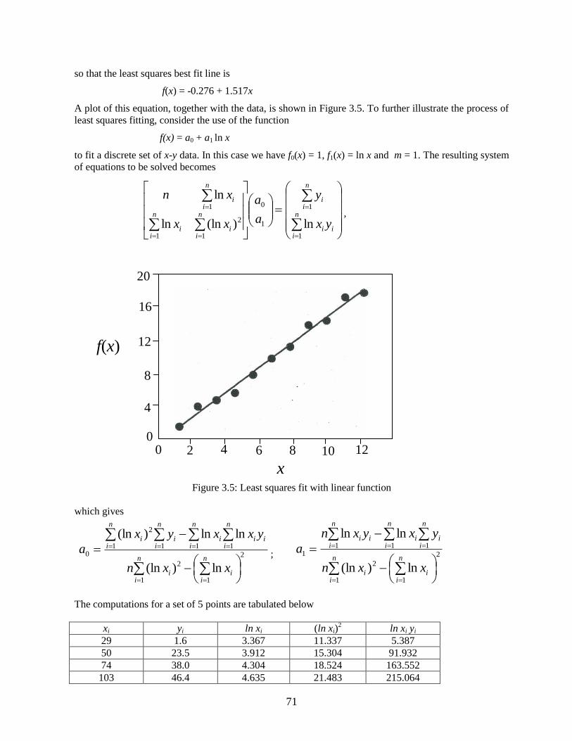
so that the least squares best fit line is
f(x) = -0.276 + 1.517x
A plot of this equation, together with the data, is shown in Figure 3.5. To further illustrate the process of
least squares fitting, consider the use of the function
f(x) = a0 + a1 ln x
to fit a discrete set of x-y data. In this case we have f0(x) = 1, f1(x) = ln x and m = 1. The resulting system
of equations to be solved becomes
n
iii
n
ii
n
ii
n
ii
n
ii
yx
y
a
a
xx
xn
1
1
1
0
1
2
1
1
ln)(lnln
ln
,
Figure 3.5: Least squares fit with linear function
which gives
2
11
2
1 111
2
0
ln)(ln
lnln)(ln
n
ii
n
ii
n
i
n
iii
n
iii
n
ii
xxn
yxxyx
a ; 2
11
2
1 111
ln)(ln
lnln
n
ii
n
ii
n
i
n
ii
n
iiii
xxn
yxyxn
a
The computations for a set of 5 points are tabulated below
xi yi ln xi (ln xi)2 ln xi yi
29 1.6 3.367 11.337 5.387
50 23.5 3.912 15.304 91.932
74 38.0 4.304 18.524 163.552
103 46.4 4.635 21.483 215.064
x
f(x)
2 4 6 8 12 10
4
8
12
16
20
0 0
72
118 48.9 4.771 22.762 233.302
=158.4 =20.989 =89.410 =709.237
Using (3.32) and (3.33) these values give
125.111989.20416.895
237.709989.204.15841.8920
a
019.34989.2041.895
4.158989.20237.709521
a . . .
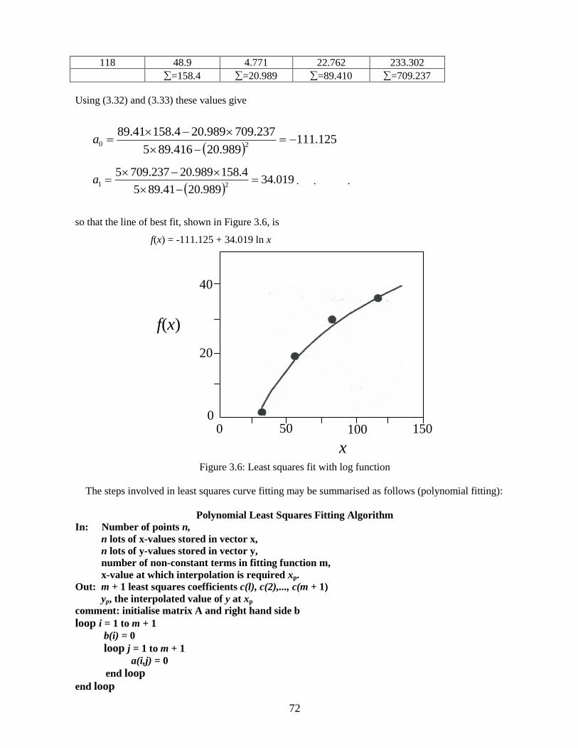
so that the line of best fit, shown in Figure 3.6, is
f(x) = -111.125 + 34.019 ln x
Figure 3.6: Least squares fit with log function
The steps involved in least squares curve fitting may be summarised as follows (polynomial fitting):
Polynomial Least Squares Fitting Algorithm
In: Number of points n,
n lots of x-values stored in vector x,
n lots of y-values stored in vector y,
number of non-constant terms in fitting function m,
x-value at which interpolation is required xp.
Out: m + 1 least squares coefficients c(l), c(2),..., c(m + 1)
yp, the interpolated value of y at xp
comment: initialise matrix A and right hand side b
loop i = 1 to m + 1
b(i) = 0
loop j = 1 to m + 1
a(i,j) = 0
end loop
end loop
x
f(x)
50 100 150
20
40
0 0
73
comment: loop over number of points
loop k = 1 to n
comment: form matrix A and right hand side b
loop i = 1 to m + 1
b(i) = b(i) + x(k)^(i-1) y(k)
loop j = 1 to m + 1
a(i,j) = a(i,j) + x(k)^(i-1) x(k)^(j-1)
end loop
end loop
end loop
comment: compute coefficients c for least squares function
solve the linear system A c = b for c
comment: compute function values at xp
Algorithm 3.2: Polynomial least squares fitting
Computer Lab. MATLAB tutorial 1: Curve fitting.
First, we consider the following problem: The stopping distance of a car on a certain road is
presented in the Table below as a function of initial velocity:
Velocity (km/h) Stopping Distance (m)
33.01 4.69
33.01 4.05
41.06 6.86
49.11 10.33
57.11 15.61
65.21 22.28
71.81 28.04
78.57 34.44
85.81 39.01
93.06 43.46
>> x = [33.01 33.01 41.06 49.11 57.16 65.21 71.81 78.57 85.81 93.06]’
>> y = [4.69 4.05 6.86 10.33 15.61 22.28 28.04 34.44 39.01 43.46]’
We wish to fit the stopping distance (y) as a linear function of velocity (x). In order to do this,
in this exercise we will use two intrinsic MATLAB functions:
74
Function Description
polyfit Polynomial curve fit.
polyval Evaluation of polynomial fit.
The MATLAB polyfit function generates a ‘best fit’ polynomial of a specified order for a
given set of data. For a linear fit, we will use:
>> p = polyfit (x,y,1)
where ‘1’ means linear or first order. (‘1’ is replaced by ‘2’ for a quadratic or second order fit
etc).
This returns:
p =
0.6762 -20.2188
To evaluate the fitted polynomial at the velocity values (x) and plot the fit against the
observed data we use:
>> y1 = polyval (p,x);
plot (x,y,'+',x,y1,'-'), grid on
In the resulting figure, you will see presented the original data and the linear fit. We can see
that the linear fit is not really working well for the given set of data. How do we define the
‘goodness of fit’?
By analyzing residuals. A measure of the goodness of fit is the residual, the difference
between the observed and the predicted data. Compare the residuals for the linear and
quadratic fits:
>> p = polyfit (x,y,2)
p =
0.0041 0.1765 -6.6235
>> y2 = polyval (p,x);
res1 = y – y1;
res2 = y – y2;
plot (x, res1, '+', x, res2, 's')
We can see that the quadratic fit is better than the linear one.
75
Exercises
(a) Calculate the norm of the residuals in the above example using the following expression:
n
i
iiY xΨyres1
2))((||
where )(xΨ is the fitting function.
(b) Repeat the linear fitting procedure for the function Y = y . Present a plot of the data (y)
and the fitting function ( 2Ψ ) and the residual. Calculate the norm of the residual. Compare
your results with the quadratic fit findings obtained above. What is your conclusion?
(c) Can you suggest any physical reason why the linear fit (with Y = y) is not a good one to
describe the stopping distance of a car as a function of velocity?
(Consider equations of motion with a constant deceleration.)
Computer Lab. MATLAB tutorial 2: Curve fitting cont.
Now we wish to use MATLAB to determine the least squares coefficients a0 and a1 for the
straight line of best fit to the x,y-data contained in the following m-file example5:
function lsq_data = example5() lsq_data = [1 1.3; 2 3.5; 3 4.2; 4 5.0; 5 7.0; 6 8.8; 7 10.1; 8 12.5; 9 13.0; 10 15.6; 11 16.1];
Running this m-file gives
>>z=example5
z =
1.0000 1.3000
2.0000 3.5000
3.0000 4.2000
4.0000 5.0000
5.0000 7.0000
6.0000 8.8000
7.0000 10.1000
8.0000 12.5000
9.0000 13.0000
10.0000 15.6000
11.0000 16.1000
z can be split into a column vector x according to:

76
>> x=z(:,1)
x =
1
2
3
4
5
6
7
8
9
10
11
and similarly for y.
We use equation (3.29) of the Notes. The easiest way for MATLAB to find a0 and a1 is by
backslash division using the following linear system of two equations:
,10 ii ynaxa
.1
2
0 iiii yxxaxa
which can be written as
y
xy
a
a
x
xx
1
02
1
with nxx i / etc. By a suitable determination of A, and b given by:
>> b=[ mean(x.*y ) mean(y)]'
where the ' after ] produces a column vector. The vector coeff = [a0, a1]’ is then obtained by:
>> coeff=A\b
coeff =
1.5173
-0.2764
Exercises
(a) Determine the column vector y from the data in example5.m.
(b) Set up the matrix A.
(c) Solve for coeff.

77
(d) Now assume that x is an independent variable and y is the dependent one. Find the
new least squares coefficients c0 and c1 for the straight line x = c0 y + c1.
(e) Compare two lines of the linear best fit graphically. Compare the corresponding
coefficients and the residuals.


