Age-Period-Cohort Models

J Clin Epidemiol Vol. 52, No. 6, pp. 569–583, 1999Copyright © 1999 Elsevier Science Inc. All rights reserved.

0895-4356/99/$–see front matterPII S0895-4356(99)00033-5

Age-Period-Cohort Models: A Comparative Study of Available Methodologies

Chris Robertson,* Sara Gandini, and Peter Boyle

Division of Epidemiology and Biostatistics, European Institute of Oncology, Milano, Italy

ABSTRACT.

This article compares the estimates produced by a number of solutions to the identifiabilityproblem in age-period-cohort models using a series of disease rates with known structure. The results suggest thatonly those methods that are based on the estimable functions such as curvatures can be recommended for use inall circumstances. The other common approaches that give parameter estimates that are easier to interpret allhave induced bias in the estimates. In particular methods based on the minimization of a penalty function toachieve identifiability are only of use if there is no change in the rates with time. Any drift in the rates tends tobe expressed as a cohort-based trend. The methods based on individual records introduce a bias if there is astrong age effect in the direction of a decreasing cohort trend and a compensating increase based on periodeffects. The nonparametric testing method has little power to detect trends in the rates in small tables butascribes a strong drift in the rates to both period and cohort trends. With careful interpretation, all methods

estimate nonlinear components correctly.

J

CLIN

EPIDEMIOL

52;6:569–583, 1999. © 1999 Elsevier Science Inc.

KEY WORDS.

Age-period-cohort models, chronic disease rates, poisson regression, simulation

AGE-PERIOD-COHORT MODELS AND ASSUMPTIONS

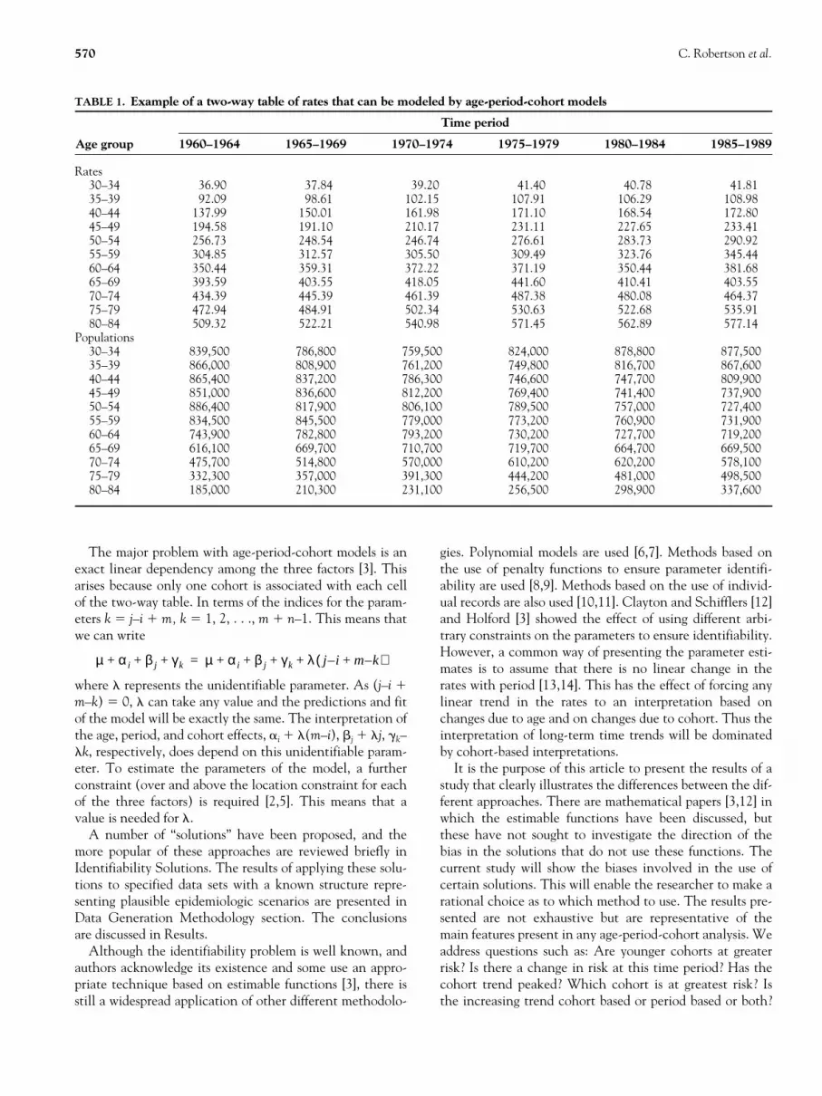
Age-period-cohort models are routinely used in descriptiveepidemiology to analyze trends in disease incidence andmortality [1]. They are used as a means of summarizing theinformation in a two-way table of disease rates classified byage group and time period, such as in Table 1. In this table,the birth cohorts form the diagonals with the oldest cohortat the bottom left-hand corner (individuals aged 80–84 in1960–1964 were born in 1874–1884), and the youngest co-hort at the top right-hand corner, born in 1951–1959. Birthcohort can be thought of as a restricted version of a moregeneral age-by-period interaction.

One aim of fitting age-period-cohort models is to assessand estimate the effects of three factors on the rates [2,3].The age effect represents the differing risks associated withdifferent age groups. Both the time period effect and thebirth cohort effect seek to explain the changes in the ratesassociated with time. The period effect represents a changein rate that is associated with all age groups simultaneously.The cohort effect is associated with a change in rates in succes-

sive age groups in successive time periods. The latter two ef-fects are the important ones in the context of time trends indisease rates. Period effects manifest themselves as a result of,for example, a change in treatment that would reduce mortal-ity in all ages at the same time, or by exposure to a carcinogenat a particular time again affecting all ages simultaneously, orpossibly by a change in registration procedure. Cohort effectsare associated with long-term habits or long-term exposureswhereby different generations are exposed to different risks.

Only age-period-cohort models that fall into the class ofgeneralized linear models are considered here. The assump-tions usually made are [4]:

1. The number of cases in age group

i

at time period

j

is de-noted

y

ij

and is a realization of a Poisson random variable,mean

u

ij

, where

i

5

1, . . . ,

m

and

j

5

1, . . .,

n

. The num-ber of age groups is

m

and the number of periods is

n

.2. The number of persons at risk in age group

i

at period

j

(

N

ij

) is a fixed known value.3. The logarithm of the expected rate is a linear function of

the effects of age group, time period, and birth cohort:

where

m

represents the mean effect,

a

i

represents the ef-fect of age group

i

,

b

j

the effect of time period

j

, and

g

k

the effect of the

k

th birth cohort.

E rij[ ]( )lnθij

Nij-------

ln µ α i β j γk+ + += =

*Address correspondence to: Dr. C. Robertson, European Institute ofOncology, Division of Epidemiology and Biostatistics, via Ripamonti 435,20141 Milano, Italy.

Accepted for publication on 12 February 1999.

570

C. Robertson

et al.

The major problem with age-period-cohort models is anexact linear dependency among the three factors [3]. Thisarises because only one cohort is associated with each cellof the two-way table. In terms of the indices for the param-eters

k

5

j

–

i

1

m, k

5

1, 2, . . .,

m

1

n

–1. This means thatwe can write

where

l

represents the unidentifiable parameter. As (

j–i

1

m

–

k

)

5

0,

l

can take any value and the predictions and fitof the model will be exactly the same. The interpretation ofthe age, period, and cohort effects,

a

i

1

l

(

m

–

i

),

b

j

1

l

j

,

g

k

–

l

k

, respectively, does depend on this unidentifiable param-eter. To estimate the parameters of the model, a furtherconstraint (over and above the location constraint for eachof the three factors) is required [2,5]. This means that avalue is needed for

l

.A number of “solutions” have been proposed, and the

more popular of these approaches are reviewed briefly inIdentifiability Solutions. The results of applying these solu-tions to specified data sets with a known structure repre-senting plausible epidemiologic scenarios are presented inData Generation Methodology section. The conclusionsare discussed in Results.

Although the identifiability problem is well known, andauthors acknowledge its existence and some use an appro-priate technique based on estimable functions [3], there isstill a widespread application of other different methodolo-

µ α i β j γk+ + + µ α i β j γk λ+ + + + j–i m–k+( )=

gies. Polynomial models are used [6,7]. Methods based onthe use of penalty functions to ensure parameter identifi-ability are used [8,9]. Methods based on the use of individ-ual records are also used [10,11]. Clayton and Schifflers [12]and Holford [3] showed the effect of using different arbi-trary constraints on the parameters to ensure identifiability.However, a common way of presenting the parameter esti-mates is to assume that there is no linear change in therates with period [13,14]. This has the effect of forcing anylinear trend in the rates to an interpretation based onchanges due to age and on changes due to cohort. Thus theinterpretation of long-term time trends will be dominatedby cohort-based interpretations.

It is the purpose of this article to present the results of astudy that clearly illustrates the differences between the dif-ferent approaches. There are mathematical papers [3,12] inwhich the estimable functions have been discussed, butthese have not sought to investigate the direction of thebias in the solutions that do not use these functions. Thecurrent study will show the biases involved in the use ofcertain solutions. This will enable the researcher to make arational choice as to which method to use. The results pre-sented are not exhaustive but are representative of themain features present in any age-period-cohort analysis. Weaddress questions such as: Are younger cohorts at greaterrisk? Is there a change in risk at this time period? Has thecohort trend peaked? Which cohort is at greatest risk? Isthe increasing trend cohort based or period based or both?

TABLE 1.

Example of a two-way table of rates that can be modeled by age-period-cohort models

Age group

Time period

1960–1964 1965–1969 1970–1974 1975–1979 1980–1984 1985–1989

Rates30–34 36.90 37.84 39.20 41.40 40.78 41.8135–39 92.09 98.61 102.15 107.91 106.29 108.9840–44 137.99 150.01 161.98 171.10 168.54 172.8045–49 194.58 191.10 210.17 231.11 227.65 233.4150–54 256.73 248.54 246.74 276.61 283.73 290.9255–59 304.85 312.57 305.50 309.49 323.76 345.4460–64 350.44 359.31 372.22 371.19 350.44 381.6865–69 393.59 403.55 418.05 441.60 410.41 403.5570–74 434.39 445.39 461.39 487.38 480.08 464.3775–79 472.94 484.91 502.34 530.63 522.68 535.9180–84 509.32 522.21 540.98 571.45 562.89 577.14

Populations30–34 839,500 786,800 759,500 824,000 878,800 877,50035–39 866,000 808,900 761,200 749,800 816,700 867,60040–44 865,400 837,200 786,300 746,600 747,700 809,90045–49 851,000 836,600 812,200 769,400 741,400 737,90050–54 886,400 817,900 806,100 789,500 757,000 727,40055–59 834,500 845,500 779,000 773,200 760,900 731,90060–64 743,900 782,800 793,200 730,200 727,700 719,20065–69 616,100 669,700 710,700 719,700 664,700 669,50070–74 475,700 514,800 570,000 610,200 620,200 578,10075–79 332,300 357,000 391,300 444,200 481,000 498,50080–84 185,000 210,300 231,100 256,500 298,900 337,600

Age-Period-Cohort Models

571

In all cases, we assume that there are age effects, as most ta-bles of disease incidence or mortality rates show evidence ofgreater risk among older people. The investigations arebased on the data in Table 1.

INDENTIFIABILITY SOLUTIONS

There are three broad classes of solutions within the age-period-cohort models other than those that are based on ar-bitrary linear constraints [15]. The first is based on the use ofa penalty function that is minimized to derive the necessaryextra linear constraint. Second, there are the methods thatrely on having individual records of cases so that a three-wayage-period-cohort table can be constructed. Finally, there arethe methods that concentrate solely on the estimable func-tions. A nonparametric-test–based method for establishing ifthere were cohort-based trends is also discussed here [16].This does not fit into the general modeling methods of theothers but is used here, as the method does have some appli-cation in the detection of trends in the rates.

Penalty Function Approach

The nonidentifiability arises because there is a linear rela-tionship among the parameters of the age-period-cohortmodel. Osmond and Gardner [17] and Decarli and La Vec-chia [18] suggested that a constraint may be imposed by en-suring that a penalty function is minimized. This will resultin an estimated value for

l

and so will yield identifiable pa-rameters. The steps of the method are the following:

1. Fit each of the three two factor models (age-period, age-cohort, period-cohort) and store the three sets of param-eter estimates.

2. Fit the full age-period-cohort model using any arbitraryconstraint on the parameters such as specifying that theeffects of the first and last period should be equal.

3. Construct the penalty function that is the sum of thesquares of the differences between the parameters ofeach of the three two-factor models and the full three-factor model weighted by a measure of goodness of fit ofeach of the three two-factor models, such as the devi-ance.

4. This penalty function is a function of

l

, and by minimiz-ing the function over all possible values of

l

, an esti-mated value of

l

is obtained.5. This value of

l

is then used to correct the parameters ofthe full age-period-cohort model (item 2 in this list) togive the identifiable estimates.

There are slight differences between the two approaches,and in this study, only the Decarli and La Vecchia solutionwill be used, as both methods have the same type of con-straint. Decarli and La Vecchia [18] also provide general-ized linear interactive modeling (GLIM) [19] macros for fit-ting their version.

Individual Records Approach

Robertson and Boyle [20] attempted to overcome the non-identifiability problem by using the individual records ofcases’ yearly population figures and forming a three-way ta-ble of age group, time period, and birth cohort [21]. Thisprocedure also has the advantage of having unique birth co-horts that do not overlap with each other.

The fitted model is

where

i

5

1, . . . ,

m

,

j

5

1, . . . ,

n

k

5

j–i

1

m

, for the oldercohort and

k

5

j–i

1

m

1

1 for the younger cohort. Asthere are two cohorts associated with each (

i, j

) combina-tion, the exact linear dependency between the parameterindices is broken. Within the same assumptions as discussedin the first section of this article, this model is identifiable.This model is easy to fit within any standard GLIM pro-gram [19], as no other special procedures are required toachieve identifiable parameters.

This age-period-cohort model often does not provide avery good fit to the data. As there is underestimationamong the younger cohort within an age group and overes-timation among the older cohort within the age group [22].This approach has also been criticized by a number of au-thors [12,23] as the assumption of a common age effectwithin the two cohorts associated with each cell of the two-way table of rates is invalid. An extension has been consid-ered [22] where the age factor has separate parameters torepresent the age effects for the older and younger cohortswithin an age group. This is, in effect, an extended agemodel, which can also be written as follows:

where

k

9

5

1 for the younger cohort within age group

i

and

k

9

5 2 for the older cohort.Here there are 2m–1 parameters for the age effects, and

n–1 for the period effects. As only cohort 1 is present in pe-riod 1 in age group m, k9 5 2, and cohort m 1 n is onlypresent in period n in age group 1, k9 5 1, the constraintsg1 5 g2 and gm1n 5 gm1n–1 are imposed. Without this con-straint, all age-period-cohort models fit the youngest cohortin the (1, n) cell and the oldest cohort in the (m, 1) cell ex-actly with residuals of zero. This constraint serves a dualpurpose; it ensures identifiability and reduces the influenceof two of the most extreme cells. Again, this model requires nospecial procedures to fit it, as all parameters are identifiable.

Deviations, Curvatures, and Drift

Holford [4], Clayton and Shifflers [12], Tango and Kura-shina [24] and Tarone and Chu [25] concentrated only onthe estimable functions and do not make any attempt toimpose any constraints to ensure identifiability. Claytonand Shifflers [12] suggest that the two degrees of freedomassociated with the linear trends be partitioned into two

E rijk[ ]( )ln µ α i β j γk+ + +=

E rijk[ ]( )ln µ α ik ′ β j γk+ + +=

572 C. Robertson et al.

components. One is the linear age effect, and the other isthe “drift.” The rationale for this is that age is assumed to bethe dominant factor. The time and cohort linear effects arelinked together and are known as the linear drift. Holford[4] showed that identifiable linear terms in the model wereaL 1 bL, aL 1 gL, or bL 1 gL, where aL, bL, and gL are thelinear effects of age, period, and cohort, respectively. Thelatter term is the drift of Clayton and Shifflers [12], whereasthe others are the cross-sectional age effect and longitudi-nal age effect, respectively.

For these approaches, the easiest way of estimating theparameters is to fit the age-period-cohort model with anyarbitrary constraint and then to transform the estimatesinto the curvatures and deviations. The curvatures of theestimates are the second differences of the parameter esti-mates, for example a1–2a2 1 a3 [12]. These second differ-ences are all estimable and do not depend on the linearconstraint used. Holford [4] showed that the deviationsfrom linearity were estimable. The deviations for age arethe residuals from a linear regression of the estimated ageeffects (ai obtained using any arbitrary constraint for identi-fiability) on the age index (i). Similarly for the period andcohort deviations and curvatures.

The Holford [4] parameters represent deviations from lin-earity, and, consequently, for each factor, the parameter esti-mates sum to zero. Thus the deviations are not independent ofeach other. The curvatures are local curvatures and are not in-fluenced by the curvatures at intervals far apart, although cur-vatures for adjacent intervals are correlated, as they have esti-mated effects in common. In fact, the curvatures and thedeviations are linearly related, and so only the Holford [4] ap-proach is used here, as the deviations from linearity have aninterpretation that is slightly closer to the estimated effectsfrom the penalty function and the individal-records ap-proaches than the second-order differences of the parameters.

Testing Method

A nonparametric testing method has been proposed [16] foruse in apportioning any trends to birth cohort or time period.The method is simply based on a comparison of rates amongindividuals in the same age group from one time period tothe next, or one birth cohort to the next. Thus, for example,the rate in the (1,1) cell of Table 1 is compared to the rate inthe (1,2) cell and the rate in the (1,2) cell to the rate in the(1,3) cell. Under the assumption of no period or cohort ef-fects, then the probability of a decrease in the rates is 0.5,and the distribution of the number of decreases can be enu-merated leading to a nonparametric test. This does not fit inwith the generalized linear model of the other methods but isa method that can be used to partition trends between periodand cohort and so is worthy of study here.

Full details of this approach are provided [16]. Briefly,the m 3 n table of rates, is rewritten as an m 1 n–1 3 n ta-ble, where the rates are classified by cohort and period. The

changes in the rates over the same age group are then as-sessed by comparing rij with r(i11)(j11) and recording 0 ifthere has been an increase in the rates and 1 if there hasbeen a decrease. Each row is a comparison of cohort k withcohort (k 1 1), and each column a comparison of period jwith (j 1 1), both among individuals in the same age group.

The number of decreases in the columns are recorded. Ifthe rates do not change systematically with period, then theprobability of a decrease is 0.5, and as there are n age groups,there are n comparisons in each column of the matrix. Thus,the number of decreases in a column will follow a binomialdistribution, as the comparisons of the different age groupsare independent. Within a particular row, there are between1 and (m–1) comparisons that can be made for any pair of ad-jacent cohorts. The cohorts are combined in blocks, princi-pally to obtain a comparison on a larger number of compo-nents [16]. Although the exact distribution of the number ofdecreases in the cohort comparison blocks requires enumera-tion, the expected value and standard deviation can easily beevaluated [16]. T-statistics can he calculated and P valuesmay be obtained from a normal approximation, which is notreally valid, as there are too few components. In this study,we use cohorts in blocks of three, which gives a 15-year spanfor the cohort, similar to Tarone and Chu [16]. An exampleof the calculations is given in Table 2.

In the absence of any period effects, one would concludethat there were different patterns of incidence in differentcohorts if all the t-values associated with the period compari-sons were close to zero whereas those associated with the co-hort comparisons were not. Correspondingly, in the absenceof cohort effects, there is evidence of period changes in therates if the t values for cohort are close to zero but those asso-ciated with period comparisons are not. The key point is thatif there are both period and cohort effects, it is not possible toseparate out the effects. In Tarone and Chu [16], the columndecreases were close to those expected and so there were noperiod effects; thus, they were able to conclude the existenceof cohort-based trends. Tarone and Chu [16] also used dataon a much finer scale and initially had data in 2-year agegroups and time periods, compared to the 5-year intervalshere. Using the finer scale gives a larger number of compo-nents to the block and column totals.

With this approach, we are looking for large t-values asso-ciated with period effects and with cohort effects. While theyare not directly comparable to the estimates discussed earlierin Penalty Function Approach and in Individual RecordsApproach or the deviations described in Deviations, Curva-tures, and Drift, they contain similar information, and thepatterns among the period and cohort t-values should be thesame as among the period and cohort effects and deviations.

DATA GENERATION METHODOLOGY

The female population of Scotland over the period 1960 to1989 for ages 30–84 in 5-year age groups and time periods

Age-Period-Cohort Models 573

TA

BL

E 2

.C

alcu

lati

ons

for

the

Tar

one

and

Ch

u N

on P

aram

etri

c T

esti

ng

Met

hod

usi

ng

the

data

fro

m T

able

1

Coh

ort

mid

poin

t

Tim

e pe

riod

mid

poin

tR

ows

Blo

cks

of t

hre

e

t-V

alu

eN

um

ber

decr

ease

sE

xpec

ted

nu

mbe

rSt

anda

rdde

viat

ion

Nu

mbe

rde

crea

ses

Exp

ecte

dn

um

ber

Stan

dard

devi

atio

n19

6219

6719

7219

7719

8219

87

1880

509.

32—

——

——

00.

50.

5018

8547

2.94

522.

21—

——

—0

1.0

0.71

03

1.00

23.

0018

9043

4.39

484.

9154

0.98

——

—0

1.5

0.87

14.

51.

192

2.94

1895

393.

5944

5.39

502.

3457

1.45

——

12.

01.

002

6.0

1.35

22.

9519

0035

0.44

403.

5546

1.39

530.

6356

2.89

—1

2.5

1.12

37.

01.

472

2.72

1905

304.

8535

9.31

418.

0548

7.38

522.

6857

7.14

12.

51.

127

7.5

1.55

20.

3219

1025

6.73

312.

5737

2.22

441.

6048

0.08

535.

915

2.5

1.12

107.

51.

551.

6119

1519

4.58

248.

5430

5.50

371.

1941

0.41

464.

374

2.5

1.12

97.

51.

550.

9619

2013

7.99

191.

1024

6.74

309.

4935

0.44

403.

550

2.5

1.12

47.

51.

552

2.25

1925

92.0

915

0.01

210.

1727

6.61

323.

7638

1.68

02.

51.

121

7.5

1.55

24.

1819

3036

.90

98.6

116

1.98

231.

1128

3.73

345.

441

2.5

1.12

27.

01.

472

3.40

1935

—37

.84

102.

1517

1.10

227.

6529

0.92

12.

01.

003

6.0

1.35

22.

2219

40—

—39

.20

107.

9116

8.54

233.

411

1.5

0.87

34.

51.

192

1.26

1945

——

—41

.40

106.

2917

2.80

11.

00.

712

3.0

1.00

21.

0019

50—

——

—40

.78

108.

980

0.5

0.50

1955

——

——

—41

.81

Num

ber

22

19

2Ex

pect

ed5.

55.

55.

55.

55.

5St

anda

rdde

viat

ion

1.66

1.66

1.66

1.66

1.66

t-V

alue

22.

112

2.11

22.

712.

112

2.11

The

num

ber o

f row

dec

reas

es is

a c

ompa

riso

n of

the

sam

e ag

e gr

oup

in o

ne ro

w a

nd in

the

subs

eque

nt. T

he fi

rst e

ntry

is 5

09.3

2 co

mpa

red

to 5

22.2

1, w

hich

is a

n in

crea

se o

f rat

es a

mon

g 80

–84-

year

-old

s. In

th

e ne

xt ro

w th

ere

are

two

com

pari

sons

of 7

5–79

-yea

r-ol

ds (

both

are

incr

ease

s). T

he e

xpec

ted

num

ber o

f row

dec

reas

es a

nd st

anda

rd d

evia

tion

are

from

the

bino

mia

l dis

trib

utio

n.T

he ro

w d

ecre

ases

in b

lock

s of t

hree

are

obt

aine

d by

sum

min

g up

the

num

ber o

f dec

reas

es in

the

corr

espo

ndin

g bl

ocks

of t

hree

com

pari

sons

. The

exp

ecte

d va

lues

and

stan

dard

dev

iati

ons a

re o

btai

ned

by

sum

min

g up

ove

r the

inde

pend

ent c

ompa

riso

ns w

ithi

n th

ese

bloc

ks.

The

Col

umn

decr

ease

s giv

e th

e nu

mbe

r of d

ecre

ases

in o

ne p

erio

d co

mpa

red

to th

e ne

xt, c

ompa

ring

cel

ls o

f the

sam

e ag

e gr

oup.

In th

e fir

st tw

o co

lum

ns th

ere

are

2 de

crea

ses i

n th

e 19

10 a

nd 1

915

co-

hort

s. T

he e

xpec

ted

valu

es a

nd st

anda

rd d

evia

tion

s com

e fr

om th

e bi

nom

ial d

istr

ibut

ion.


was used as the basis of the calculation of the expected num-bers of cases (Table 1). Two separate methods were used togenerate the expected rates. The curvature approach [12] ismathematically correct and can be used to generate the dataaccording to any predefined structure. Specifically, data withage effects similar to those obtained in many cancer siteswere generated with and without any drift, with and withoutany nonlinear period and cohort curvatures using

(1)

E rijk[ ]( )ln µ αL i 1–( ) γL k m–( ) αPlxPlil 2=

n 1–

∑

βAlxAljl 2=

m 1–

∑ γClxClkl 2=

m n 2–+

∑

+ + +

+ +

=

In the above, j–1 represents the linear age effect, k–m thecohort drift effect, both centered on the (1, 1) cell, and thex terms are explanatory variables representing the curva-tures. Values are assigned to aL, gL, aPl, bAl, gCl to representvarious scenarios for the mean rates. Although drift is rep-resented by a linear cohort term, it could equally well berepresented by a linear period term and exactly the samemean values would be obtained, provided aL is replaced byaL–gL, as k 5 j–i 1 m.

To evaluate the individual-records approach [20], amodel with linear age and drift terms together with qua-dratic, and other nonlinear age, period, and cohort effectswas used to generate individual level data on a single-yearbasis, which was then combined into two- and three-waytables in 5-year groups. This method was chosen in prefer-ence to the more general drift and curvature method for thetwo-way tables because of the large age, period, and cohortranges that would have required very many parameters us-ing a model such as 1. The model was as follows:

(2)

f(a) is a function of age and was either a linear or logarith-mic function. The terms pD and cD are dummy variablesthat pick out the period 1970–1974 and the cohort 1915–1924 for nonlinear disturbances to the drift. If b3 and g3 areboth zero, then any curvatures are smooth, taking the samevalue in all periods or cohorts as we have a quadratic model.

Two approaches were adopted—a study of expected val-ues and a simulation study. In the former, the expectednumber of cases was calculated from Equations (1) or (2)and the populations in Table 1. These were used as the re-sponse variables when fitting the age-period-cohort modelsto give the expected values of the parameters. When theTarone and Chu method is applied to the tables of ex-pected rates under situations of a trend in the rates, thenthe number of decreases will always take the maximum orminimum value depending on the direction of the trend.This means that the t-values illustrated will be the maxi-mum, or minimum, possible. In the simulation study, 100data sets were generated and the average and standard devi-

E rapc[ ]( )ln µ α f a( ) γc α2a2

β2 p2 γ2c2 β3 pD γ3cD+ + +

+++ +=

TABLE 3. Specified parameter values for Two Way Tablesimulations

Figure 1 Figure 2 Figure 3

Intercept 29.63 29.63 29.63Longitudinal age 0.25 0.25 0.25Drift 0.14 0 0.14Age curvatures

3237 20.1 20.1 20.142 20.1 20.1 20.147 20.1 20.1 20.152 20.1 20.1 20.157 20.1 20.1 20.162 20.1 20.1 20.167 20.1 20.1 20.172 20.1 20.1 20.177 20.1 20.1 20.182

Period curvatures19621967 0 0 01972 0 0 01977 0 20.3 20.31982 0 0 01987

Cohort curvatures18801885 0 0 01890 0 0 01895 0 0 01900 0 0 01905 0 0.3 0.31910 0 0 01915 0 0 01920 0 0 01925 0 20.3 20.31930 0 0 01935 0 0 01940 0 0 01945 0 0 01950 0 0 01955

TABLE 4. Specified parameter values for Individual Recordsimulations

Figure 4 Figure 5 Figure 6 Figure 7

Intercept 29 29 29 29Log age 1 1.5 1 1Drift 0.005 0.005 0.005 0.005Quadratic age 0 0 0 0Quadratic period 0 0 0 0Quadratic cohort 0 20.0005 0 20.0004Non-linear period 0 0 0.05 0.05Non-linear cohort 0 0 20.1 20.1


ation of the estimated parameters recorded. With this sam-ple size, the estimated standard errors for the curvatures areexpected to be within 15% of the true standard errors with95% confidence. The main reason for the simulation studywas to investigate the effect of sampling variation on thebias, and, as this was not great, most of the results presentedrefer to the expected value study only.

We expect that the curvature method [12] and conse-quently the method of Holford [4], will always return thespecified model, and we are investigating the circumstancesin which the same is true with the other three approaches.In the methods that try to achieve identifiability, the mainquestion is how the linear components are apportioned

among the three factors of age, period, and cohort. Specifi-cally, what biases are present in the estimates.

In a study of bias when there are a small number of pa-rameters, the study would be designed to move systemati-cally through a range of values for these parameters measur-ing the bias at each point and tabulating the results. Here,there is a much larger number of parameters, and we are in-terested in the qualitative results of the study. The ability ofthe different solutions to capture successfully the specifiedshapes in the table of rates, in terms of the estimated pa-rameters, is of importance. Consequently, we adopt agraphical portrayal of a small set of representative situa-tions.

FIGURE 1. Two-way table: Ageeffect, linear drift. Dots anddashes: Holford, solid line: De-carli and La Vecchia, dottedline: Tarone and Chu. Parame-ter estimates in Table 3.


RESULTS

The specified parameter estimates for the calculated dataare listed in Table 3 for the two-way tables, based on model1, and in Table 4 for the individual level approach based onmodel 2. Initially, simple models are used, and then morecomplex combinations of parameter values are specified toachieve tables that are representative of features that mightbe observed in practice. Results for a number of modelsbased on a two-way table only are illustrated in Figures 1through 3. The individual-records method [19] cannot beapplied to two-way tables, and it is compared to the othersin Figures 4 through 7.

In these figures, the Holford estimates are deviationsfrom linearity, whereas the Tarone and Chu ones are t-sta-tistics. Thus, they are not directly comparable with those ofDecarli and La Vecchia and Robertson and Boyle, whichare effects on a log(rate) scale. Any t-statistics in excess of62 indicate significant changes in the rates. Trends in thet-values may also be observed and compared with thetrends in the estimates from Decarli and La Vecchia andRobertson and Boyle. The deviations determine the shapeof the graph, and these can be compared to the shape of theestimates from the Decarli and La Vecchia and Robertsonand Boyle models. Abrupt changes in the t-statistics shouldalso be reflected in the curvatures.

FIGURE 2. Two-way table: Ageeffect, no drift, nonlinear peri-od, and cohort effects. Dots anddashes: Holford, solid line: De-carli and La Vecchia, dottedline: Tarone and Chu. Parame-ter estimates in Table 3.


In all the generated data sets, the deviation approach [4]always reveals the input structure even when the data weregenerated according to the individual-records approach.This is the expected result, as this method is mathemati-cally correct, focusing, as it does, on the estimable con-trasts, making no extra assumptions to achieve identifiabil-ity. It was included in the study as a means of checking theprocess.

If there is no drift and no nonlinear period and cohort ef-fects and only an age effect, then the deviations of Holfordare all zero as they should be (data not shown). The meth-ods of Decarli and La Vecchia and Tarone and Chu are alsosuccessful in returning the input structure. The estimated

period and cohort effects are all zero, as are the t-values forthe nonparametric approach. This situation is very unlikelyto arise in practice.

If there is linear drift but no nonlinear cohort or periodeffects (Figure 1), then the deviations of Holford are all zeroas expected. The method of Decarli and La Vecchia sug-gests that there is an increasing cohort trend and very littleperiod trend. The Tarone and Chu t-statistics are consis-tent with rates that are increasing with time. They are alllarge and negative, indicating that within an age group, therates in the later period, or younger cohort, tend to behigher than in the earlier period or older cohort. As bothperiod and cohort t-statistics are large, it is not possible to

FIGURE 3. Two-way table: ageeffect, drift, nonlinear period,and cohort effects. Dots anddashes: Holford, solid line: De-carli and La Vecchia, dottedline: Tarone and Chu. Parame-ter estimates in Table 3.


assign the drift to period or cohort and this is entirely cor-rect. One would only be tempted to assign drift to period orcohort if all the t-values for one time factor were close tozero but some were significantly different from zero for theother time factor.

When there is no drift but there are nonlinear period andcohort effects then both the Tarone and Chu approach andthe Decarli La Vecchia method return the input pattern(Figure 2). The curvatures from the Decarli and LaVecchiaapproach are identical to the Clayton and Schifflers curva-tures, as the curvatures are identifiable parameters. This canbe clearly seen at the three points of nonlinear effects, period1977, Cohorts 1905 and 1925. As drift has been constrained

to be zero here, the negative curvature in 1977 means thatthere must be an increase in the rates from 1960 to 1977 fol-lowed by a decrease. This is reflected in the t-statistics, whichare large and negative up to 1977 (rates increasing) and largeand positive immediately after this point. Similarly, theabrupt changes are noted in the cohort t-statistics.

When positive drift is added (Figure 3), the shape of theTarone and Chu t-statistics are identical to those in Figure 2for cohort and period. The Decarli and La Vecchia estimatesagain show trend in the cohorts, albeit with the curvatures inthe correct place. The period effects indicated a small butsignificant linear trend, again with the curvature in the cor-rect spot.

FIGURE 4. Three-way table: ageeffect, drift. Dots and dashes:Holford, solid line: Decarli andLa Vecchia, dotted line: Taroneand Chu, long dashed lines:Robertson and Boyle, long andshort dashed lines: Robertsonand Boyle extended age. Param-eter estimates in Table 4.


In the individual-records simulations (Figure 4) we seethat the Robertson and Boyle approach is seriously biasedin the presence of strong age effects. In this figure, the biasis illustrated in the presence of a positive drift, but this biasis present even if there is no drift. Relative to the Decarliand La Vecchia model, the age effects are underestimates,there is an increasing period effect and a decreasing cohorttrend. This is brought about by the assumption of a com-mon age effect within the old and young cohort of each agegroup. When different effects are permitted, as in the ex-tended Robertson and Boyle approach, then this bias in theage effects is corrected. The drift is, however, assigned to aperiod effect and there is no cohort drift. (The estimates are

zero and are superimposed on the Holford deviations.) TheDecarli and La Vecchia approach yields the increasing co-hort trend in the presence of drift with a slight negative pe-riod trend. The Tarone and Chu t-statistics are similar tothose in Figure 1 and indicate that the rates are changingwith respect to both cohort and period.

When there is a positive drift and a cohort curvature,(Figure 5), then clear differences between the Robertsonand Boyle extended age mode and the Decarli and La Vec-chia approach emerge. The constant cohort curvature iscorrectly obtained by all methods, but the location of theturning point is different in all three cases. With Decarliand La Vecchia it is 1935, Robertson and Boyle 1910, and

FIGURE 5. Three-way table: ageeffect, drift, cohort curvature.Dots and dashes: Holford, sol-id line: Decarli and La Vecchia,dotted line: Tarone and Chu,long dashed lines: Robertson andBoyle, long and short dashedlines: Robertson and Boyle ex-tended age. Parameter estimatesin Table 4.


Robertson and Boyle extended age 1890. This is an effect ofthe partition of the drift to the linear terms for age, period,and cohort. With Decarli and La Vecchia, this is assignedto the cohort trend, and consequently the turning point forthe cohort effects moves toward the later cohorts. With theRobertson and Boyle method, the imbalance in the ages inthe old and young cohort leads to a negative cohort trendthat is exacerbated by the positive drift that tends to be as-signed to period. Thus, the cohort turning point is shiftedtoward the older cohorts. This means that the turning pointin smoothly changing rates is not an identifiable parameter.The sawtoothing in the age effects for the extended agemodel means that there is an overcorrection of the age ef-fects within the cohort terms. The Tarone and Chu t-statis-

tics are consistent with the estimates of Decarli and LaVecchia and put the turning point at 1925–1940.

The disparity in the turning point in the cohort curva-tures still exists when there is smooth cohort curvaturespecified but no drift (no graph). The differences betweenthe methods are not as great, but it is still the case that theRobertson Boyle methods tend to place the turning pointmuch earlier than the Decarli and La Vecchia approach.

If there are nonlinear period and cohort effects, thenthese can both be picked up by all methods (Figure 6). Theinstantaneous increase in the rates in 1977 is visible in allestimates, as is the instantaneous decrease in the 1910–1920 cohort. The small positive drift induces an increasedcohort effect with the Decarli and La Vecchia method, but

FIGURE 6. Three-way table: ageeffect, little drift, nonlinear co-hort and period. Dots and dash-es: Holford, solid line: Decarliand La Vecchia, dotted line: Ta-rone and Chu, long dashed lines:Robertson arid Boyle, long andshort dashed lines: Robertsonand Boyle extended age. Parame-ter estimates in Table 4.


the extended age model appears to work well, althoughwhatever drift there is, is assigned to a period effect. TheTarone and Chu method correctly detects the abruptchanges in the rates associated with 1977 and the 1910–1920 cohort.

In Figure 7, we have the estimates with cohort curvaturesand nonlinear effects also. The situation is similar to that inFigures 5 and 6. The nonlinearities are identified, but the turn-ing point in the cohort trend depends on the method used.

Most graphs have illustrated positive drift, the resultswith negative drift are similar. So too were results that useddifferent values for the drift and curvature coefficients.While this is not an exhaustive search, the results illustratethe main differences between the solutions, and thus an in-

terpretation of them allows conclusions to be drawn aboutthe situations in which the solutions can be used.

CONCLUSIONS

In the absence of drift and non linear period and cohort ef-fects the method of Robertson and Boyle [19] gives biasedestimates of the Age, Period and Cohort effects in the di-rection of increasing period effects and decreasing cohorteffects and Age incidence curves which are not as steep.These effects are not as severe in the presence of some driftin the rates or some non linear period and cohort effects.

If there is a linear drift, then the Decarli and La Vecchia[18] approach is biased toward a linear cohort effect. This

FIGURE 7. Three-way table: ageeffect, little drift, cohort curva-ture, and non linear cohort andperiod. Dots and dashes: Hol-ford, solid line: Decarli and LaVecchia, dotted line: Tarone andChu, long dashed lines: Robert-son and Boyle, long and shortdashed lines: Robertson andBoyle extended age. Parameterestimates in Table 4.


tendency to return cohort-based trends in the presence ofdrift was consistent over a wide variety of situations, withand without nonlinear period or cohort effects. The Rob-ertson and Boyle approaches [20,22] are biased toward pe-riod-based increases compensated for by cohort-based de-creases, even if there is negative drift.

If there is any drift in the rates, then the nonparametrictesting method [16] suggests that there are both period andcohort linear effects. Nonlinear changes in the rates overperiod and cohort can be detected by this method. As allthe calculations are performed by comparing groups of thesame age, this method will not be able to provide any infor-mation about age effects. This is not a big problem, as mostage-period-cohort analyses are concerned with time trendsin the rates associated with period and cohort only. Thepower of this method is limited in small tables, as there areonly a few comparisons that can be made.

If there are nonlinear period and/or nonlinear cohort ef-fects, then all methods are capable of detecting them. Insome cases, it is harder to detect them. For example, in Figure7, the period-based nonlinearity in 1977 is harder to detectin the estimates from the Robertson and Boyle methods,whereas the cohort based changes in 1910–1920 are harderto detect in the Decarli and La Vecchia approach. However,only the deviation approach [4] is wholly successful.

The penalty function approaches [17,18] will suggest co-hort-based trends in the presence of drift. This may meanthat any period trends will be masked by this approach andwill manifest themselves as cohort trends. Nonlinear periodand cohort effects can still he detected.

The bias induced in the period and cohort effects bystrong age effects in the individual-records method [20] issevere. Although a bias correction has been proposed [22],there is much multicollinearity in the estimates. This ex-tended age model is relatively successful in the presence ofa little drift but not if there is larger drift. The collinearityin this model is manifest in the observation that in many ofthe simulated data sets, the estimated parameters of cohortand period were not significantly different from zero in theextended age model.

Curvatures are identifiable as are nonlinear deviations,so all methods can be used to detect them. The turningpoint in the rates is not an identifiable parameter, andnothing can be said about which cohort or which periodexperiences the maximum effect.

In this study, the rates were generated assuming that anage-period-cohort model is the correct model for the data.This is the correct approach when the aim of the study is tosee when the different age-period-cohort solutions arevalid. It is also of some interest to study the behavior of theestimates from the different solutions under the situationwhen an age-period-cohort model is not the correct model;for example, in tables where there is an interaction betweenage and period but it does not take the cohort shape. Insuch cases, the goodness of fit of the age-period-cohort

model and residual analysis should show that the model isnot valid for such data tables.

While the results reported are not extensive, they sum-marize the important features of the larger study. There isalso sufficient information to be able to choose between themethods. Only the methods based on curvatures or otherestimable functions can be recommended for use. These arethe Clayton Schifflers [12] approach or ones that are similarto it such as that proposed by Holford [4] and by Taroneand Chu [25]. While the deviation and curvature estimatesfrom these methods are not as easy to interpret as the pe-riod and cohort (log) relative risk effects from the othermodels, epidemiologists and statisticians should be usingthem, as they are identifiable and not subject to a relativelyarbitrary constraint.

All the other methods had bias in some data sets. Thesimulations have shown that the bias in the penalty func-tion approaches [17,18] is toward cohort-based trends. TheRobertson and Boyle [20] suggestion results in a bias towardperiod increases and cohort-based decreasing trends. Thisbias is always present, even with small amounts of drift.Also the bias is greater with the Robertson and Boyle [20]approach.

For a particular data set, the bias will produce a signifi-cant misinterpretation depending on the sample size andthe amount of drift. For tables based on large populations,even a relatively small drift may result in a conclusion ofperiod-based increases and cohort-based decreases with theRobertson and Boyle [20] approach, or cohort-based in-creases and no period changes with the Osmond and Gard-ner and Decarli and La Vecchia [17,18] approaches. Conse-quently, these methods should not be used, and theinterpretations of results of previous analyses based on thesemethods should be revised.

Holford [3] also discusses the use of trends in covariatesand nonlinear trends in the temporal variables as a meansof ensuring identifiability. This approach is of limited use,as covariates are seldom available and the use of nonlinearmodels such as log(age) can only be justified on rare occa-sions. Also the interpretation of the period and cohort ef-fects will depend heavily on the validity of the nonlinearmodel.

References1. Coleman M, Esteve J, Damiecki P, Arslan A, Renard H.

Trends in Cancer Incidence and Mortality. Lyon: IARC;1993.

2. Kupper LL, Janis JM, Karmous A, Greenberg BG. Statisticalage-period-cohort analysis: A review and critique. J ChronicDis 1985; 38: 811–830.

3. Holford TR. Analysing the temporal effects of age, period andcohort. Stat Methods Med Res 1992; 1: 317–337.

4. Holford TR. The estimation of age, period and cohort effectsfor vital rates. Biometrics 1983; 39: 311–324.

5. Fienberg SE, Mason WM. Identification and estimation of


age-period-cohort models in the analysis of discrete archivaldata. In: Schuessler KF, Ed. Sociological Methodology. SanFrancisco: Josey-Bass: 1–67.

6. Luostarinen T, Hakulinen T, Pukkala E. Cancer risk follow-ing a community based programme to prevent cardiovasculardiseases. Int J Epidemiol 1995; 24: 1094–1099.

7. Svanes C, Lie RT, Kvale S, Svanes K, Soreide O. Incidence ofperforated ulcer in western Norway, 1935–1990: Cohort- orperiod-dependent time trends? Am J Epidemiol 1995; 141:836–844.

8. Chie WC, Chen CF, Lee WC, Chen CJ, Lin RS. Age-period-cohort analysis of breast cancer mortality. Anticancer Res1995; 15: 511–515.

9. Lopez AG, Pollan M, Jimenez M. Female mortality trends inSpain due to tumours associated with tobacco smoking. Can-cer Causes Control 1993; 4: 539–545.

10. Lee WC, Lin RS. Interactions between birth cohort and ur-banisation on gastric cancer mortality in Taiwan. Int J Epide-miol 1994; 23: 252–260.

11. McNally RJ, Alexander, FE, Stains A, Cartaright RA. A com-parison of three methods of analysis for age-period-cohortmodels with application to incidence data on non-Hodgkin’slymphoma. Int J Epidemiol 1997; 26: 32–46.

12. Clayton D, Schifflers E. Models for temporal variation in cancerrates II: Age-period-cohort models. Stat Med 1987; 6: 468–481.

13. Hristova L, Dimova I, Iltcheva M. Projected cancer incidencerates in Bulgaria, 1968–2017. Int J Epidemiol 1997; 26: 469–475.

14. Reissigova J, Luostarinen T, Hakulinen T, Kubik A. Statisti-cal modeling and prediction of lung cancer mortality in theCzech and Slovak Republics, 1960–1999. Int J Epidemiol1994; 23: 665–672.

15. Robertson C, Boyle P. Age-period-cohort analysis of chronic dis-ease rates: I Modelling approach. Stat Med 1998; 17: 1302–1323.

16. Tarone RE, Chu KC. Implications of birth cohort patterns ininterpreting trends in breast cancer rates. J Nat Cancer Inst1992; 84: 1402–1410.

17. Osmond C, Gardner MJ. Age, period and cohort models ap-plied to cancer mortality. Stat Med 1982; 1: 245–259.

18. Decarli A, La Vecchia C. Age, period and cohort models: Areview of knowledge and implementation in GLIM. Riv StatApplic 1987; 20: 397–410.

19. Francis FF, Green M, Payne RD. Eds. GLIM 4 The StatisticalSystem for Generalized Linear Interactive Modelling. Oxford:Clarendon Press; 1993.

20. Robertson C, Boyle P. Age, period and cohort models. Theuse of individual records. Stat Med 1986; 5: 527–538.

21. Tango T. Statistical modelling of lung cancer and laryngealcancer in Scotland, 1960–1979. Am J Epidemiol 1988; 127:677–678. (Letter)

22. Robertson C, Boyle P. Age, period and cohort models: Acomparison of methods. In: Fahrmeir L, Francis B, GilchristR, Tutz G, Eds. Advances in GLIM and Statistical Model-ling. New York: Springer Verlag; 1992.

23. Osmond C, Gardner MJ. Statistical modelling of lung cancerand laryngeal cancer in Scotland, 1960–1979. Am J Epide-miol 1988; 129: 31–35. (Letter)

24. Tango T, Kurashina S. Age, period and cohort analysis oftrends in mortality from major disease in Japan, 1955 to 1979:Peculiarity of the cohort born in the early Showa Era. StatMed 1987; 6: 709–726.

25. Tarone RE, Chu KC. Evaluation of birth cohort patterns inpopulation disease rates. Am J Epidemiol 1996; 143: 85–91.

Documents

Age-Period-Cohort Models