AIRCRAFT AUTOPILOT DESIGN USING A SAMPLED-DATA GAIN SCHEDULING

TECHNIQUE

A Thesis Presented to

The Faculty of the

School of Electrical Engineering and Computer Science

and Fritz J . and Dolores H. Russ

College of Engineering and Technology

Ohio University

In Partial Fulfillment

of the Requirement for the Degree

Master of Science

Chao Wang

March, 1999

Acknowledgment

I would like to express my special thanks to my advisor, Dr. Douglas A. Lawrence,

for the insights he has provided to accomplish this thesis and the guidance given to

me. Il'ithout this, it is impossible for me to acconlplish this thesis.

I would like to thank Dr. Frank van Graas, Dr. LIichael Braasch and Dr. David

Bayless for agreeing to be members of my thesis committee and giving valuable sug-

gestions. Finally. I would like to thank my husband and family for the help. slipport.

and encouragement.

Contents

1 Introduction 1

. . . . . . . 1.1 Gain Scheduling Methodology for Sampled-Data Systems 3

. . . . . . . . . . . . . . . . . . . . . . . . . . . . . 1.2 Project Objective 3

. . . . . . . . . . . . . . . . . . . . . . . . . 1.3 Notation and Definitions 4

2 Sampled-Data Gain Scheduling Theory 5

2.1 Sampled-Data Gain Scheduling . 3 . . . . . . . . . . . . . . . . . . . . .

2.1.1 Family of Constant Operating Points and Parameterization . . 6

. . . . . . . . . . . 2.1.2 Parameterized Family of Linear Controllers 7

. . . . . . . . . . . . . . . . . . . . 2.1.3 Gain Scheduled Controller 10

. . . . . . . . . . . . . . . . . . . . . . . . . . . . . . . . 2.2 An Example 12

3 F-16 Aircraft Model 16

. . . . . . . . . . . . . . . . . . . 3.1 F-16 Aircraft Mathematical Model 16

. . . . . . . . . . . . . . . . . 3.2 Implementation of F-16 Aircraft Model 19

. . . . . . . . . . . . . . . . . . . . . . . . . . . . . 3.3 Design Objective 20

4 F-16 Autopilot Design With Gain Scheduling Technique 22

4.1 Constant Operating Points and Aircraft Linearization . . . . . . . . 23

. . 11

. . . . . . . . . . . . . . . . . . . . . . . . . 4.2 Linear -Alltopilot Design 27

. . . . . . . . . . . 4.2.1 Continuous-Time Linear Autopilot Design 28

. . . . . . . . . . . . . 4.2.2 Sampled-Data Linear ,4 utopilot Design 37

4.2.3 Example of Simulation with Linear Continuous-Time arid Sarriplcd-

DataAlutopilot . . . . . . . . . . . . . . . . . . . . . . . . . . 39

. . . . . . . . . . . . . . . . 3.2.4 Family of Linear -Autopilot Design 41

. . . . . . . . . . . . . . . . . . . . 4.3 Gain Scheduled Autopilot Design 46

. . . . . . . . . . . . . . . . . . 4.3.1 Pitch Attitude Hold Autopilot 46

. . . . . . . . . . . . . . . . . . . . . 4.3.2 Altitude Hold Autopilot 48

. . . . . . . . . . . . . . . . . . . . . . 4.3.3 Glide Slope *kutopilot 50

4.4 Comparison of Simulation Results of Linear Autopilot and Nonlinear

. . . . . . . . . . . . . . . . . . . . . . . . Gain Scheduled a4utopilot 51

5 Conclusions

Bibliograph,~

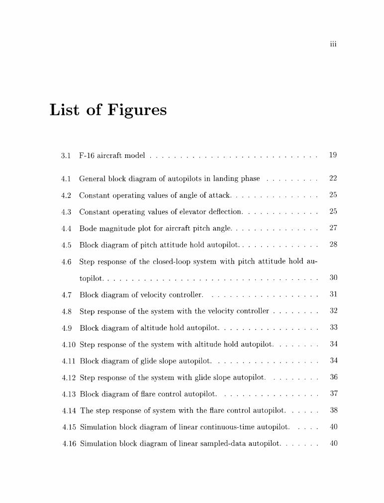
List of Figures

. . . . . . . . . . . . . . . . . . . . . . . . . 3.1 F-16 aircraft model

4.1 General block diagram of autopilots in landing phase . . . . . . . . .

. . . . . . . . . . . . . . . 4.2 Constarlt operating values of angle of att.ack

. . . . . . . . . . . . . 4.3 Const. ant operating values of elevator deflection

. . . . . . . . . . . . . . . 4.4 Bode magnitude plot for aircraft pit. ch angle

. . . . . . . . . . . . . . 4.5 Block diagram of pitch attitude hold autopilot

4.6 Step response of the closed-loop system with pitch at. titude hold au-

. . . . . . . . . . . . . . . . . . . . . . . . . . . . . . . . . . . . topilot

. . . . . . . . . . . . . . . . . . . 4.7 Block diagram of velocity controller

. . . . . . . . 4.8 Step response of t . he system with the velocity controller

. . . . . . . . . . . . . . . . . 4.9 Block diagram of altitude hold autopilot

4.10 Step response of the system with altit'ude hold autopilot . . . . . . . .

4.11 Block diagram of glide slope aut'opilot . . . . . . . . . . . . . . . . . .

4.12 Step response of' the system with glide slope autopilot . . . . . . . . .

4.13 Block diagram of flare control autopilot . . . . . . . . . . . . . . . . .

4.14 The step response of system with tmhe flare control autopilot . . . . . .

4.15 Simulation block diagram of linear continuous-time autopilot . . . . .

4.16 Simulation block diagram of linear sampled-dat'a autopilot . . . . . . .

iv

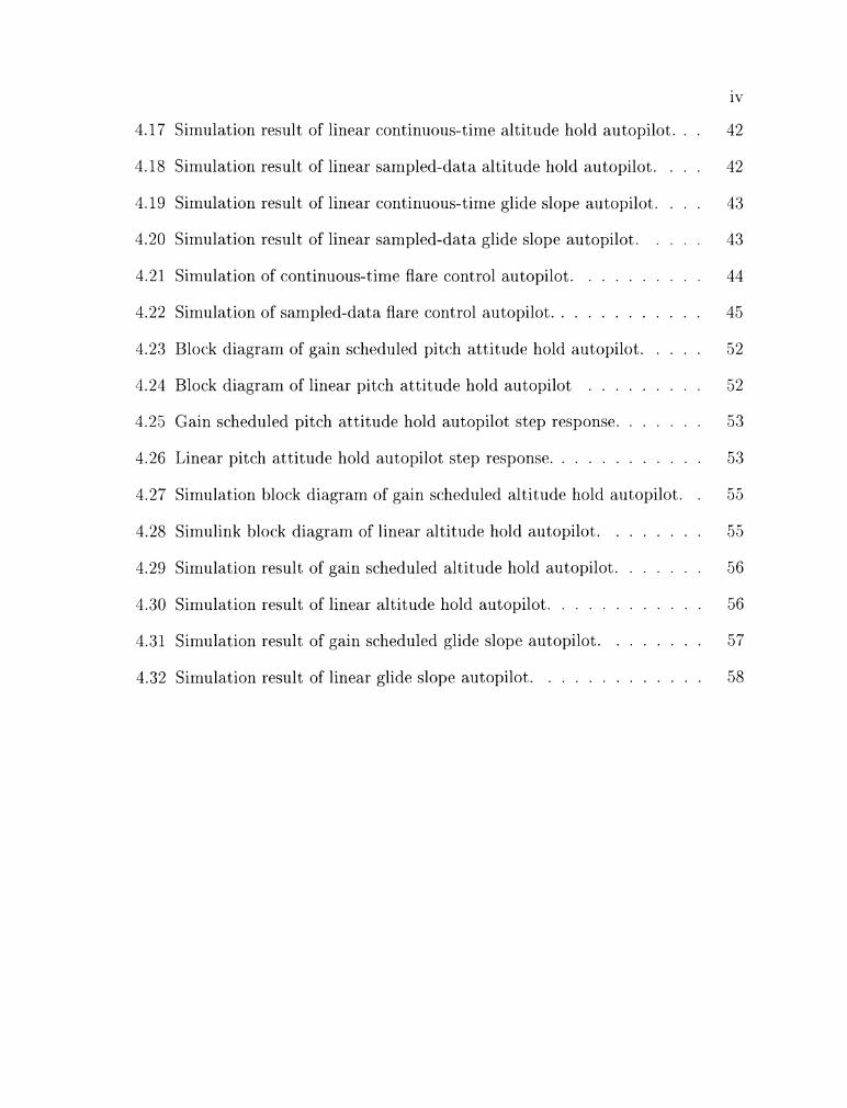
4.17 Simulation result of linear continuous-time altitude hold autopilot . . 42

4.18 Sirnulation result of linear sampled-data altitude hold autopilot . . . . 42

4.19 Siniulation result of linear continuous-time glide slope autopilot . . . . 43

4.20 Sirnulation result of linear sampled-data glide slope autopilot . . . . . 43

4.21 Simulation of continuous-time flare control autopilot . . . . . . . . . . 44

4.22 Simulation of sampled-data flare control autopilot . . . . . . . . . . . . 43

4.23 Block diagrarn of gain scheduled pitch attitude hold autopilot . . . . . 52

4.24 Block diagram of linear pitch attitude hold autopilot . . . . . . . . . 32

4.25 Gain sclleduled pitch attitude hold autopilot step response . . . . . . . 53

4.26 Linear pitch attitude hold autopilot step response . . . . . . . . . . . . 53

4.27 Siniulation block diagrarn of gain scheduled altitude hold autopilot . . 55

4.28 Sirnulink block diagram of linear altitude hold autopilot . . . . . . . . 5.3

. . . . . . . 4.29 Simulation result of gain scheduled altitude hold autopilot 56

4.30 Simulation result of linear altitude hold autopilot . . . . . . . . . . . . 56

. . . . . . . . 4.31 Sirnulation result of gain scheduled glide slope autopilot 57

. . . . . . . . . . . . . 4.32 Simulation result of linear glide slope autopilot 58

List of Tables

3.1 Test Result of F-16 Aircraft Model . . . . . . . . . . . . . . . . . . . 20

4.1 Operating Points Of rlltitude and Alach Number . . . . . . . . . . . . 24

Chapter 1

Introduction

Realistic engineering systems are often nonlinear. There are many approaches

in nonlinear control system design. such as linearization, robust control. adaptive

control, etc. Through linearizing the nonlinear system, the controller can be designed

using the approaches of linear control theory. Therefore, linearization is the rrio~t

c-ommon approach in nonlinear system design. The basic limitation of the clcsigil via

the linearization approach is the fact that the controller is guaranteed t o work onl\-

in the neighborhood of a single operating (equilibrium) point. The dynamic behavior

of a systerri changes with the operating region. -4 typical approach in this situatio~i

is gain scheduling.

I11 many situations, how the dynanlics of a system change with its operating points

car1 be identified. The system can be modeled in sudi a way that the oper atirlg points

arc parameterized by one or more variables. which are called scheduling variables. In

such situations, the system may be linearized a t several equilibrium points arid dcsign

a linear feedback controller a t each point that performs satisfactorily when the system

is operating near the respective operating points. A family of linear controllers can

be implemented as a single controller whose parameters change by rnonitoririg the

2

scheduling variables, which are intended to handle the nonlinear aspects of the design

problem. Gain scheduling is a practical method that can extend the validity of' the

coatroller operation to a set of operating points arid has been proven to be a successfill

method in many applications in nonlinear control systems design, especially in flight

control systems.

There have been numerous theoretical studies 011 the gain scheduling technique

The framework of gain scheduled controller design and analysis are proposed in [9] ,[7]

and [lo]. In [5] and [12], the methods arid examples of the application of the gain

scheduled technique in flight control systems arc. given. In [2]. Karriiner et al. intro-

ducc a nonlinear gain scheduled controller tha t preserves the input-output properties

of the linear closed-loop systems locally about each equilibrium point bv ~)rovidirig

integral action a t the inputs to the plant arid differentiating some of the measurcd out-

puts before they are fed back to the gain scheduled controller. Lawrence et al. ~~reser i t

a stability theorem for slowly varying inputs [6]. The widespread use of digital hard-

ware in controllcr implementation leads naturally to the investigation of approaches

for sampled-data gain scheduling. The framework of sampled-data gain scheduling

that builds upon previous results for the continuous-time case is presented in 131, and

a stability property of nonlinear sampled-data systems with slowing varying irlplits is

provided in [4].

I11 this thesis. the focus is on applying the sampled-data gain scheduling nic~tliod

to air craft autopilot design. Section 1.1 describes the gain scheduling concept arid

methodology. Section 1 .2 presents the objective of this thesis. Section 1.3 sets the

~iotiori and definitions used in this thesis.

3

1.1 Gain Scheduling Methodology for Sampled-Data Systems

X frame~vork for sampled-data gain scheduled controller design is proposed in [3]

The development of such controllers involves the following steps.

Compute the constant operating points of a nonlinear plant. parameterized b~

constant values of a set of scheduling variables, and obtain the corresponding

linearized plants.

For the family of linearized plants, design a parameterized farriilv of linear

discrete-time corltrollers to meet the design goals a t each operating point.

Construct a gain scheduling controller that linearizes t o the correct lincar con-

troller at each constant operating point.

lkrify the performance of the gain scheduled controller by simulation.

1.2 Project Objective

The objective of this project is to use this gain scheduling technique to dcsign

longitudinal autopilots for an F-16 fighter over an automatic landing procedure. The

experience gained will be used in Unmanned Aerial L'ehicle autopilot design in the

future.

The autopilots include pitch attitude control, altitude control, glide slop(. acaqui-

sition, arid flare control. Linear sampled-data autopilots are designed by classical

design techniques t o realize the design goals a t operating points. The family of linear

4

autopilots is obtained by linear interpolation of autopilot parameters a t interrriedi-

ate operating points. Sonlinear gain scheduled controllers are constructed such that

their linearizations match the linear autopilots performance a t each operating ~ ~ o i n t .

The six degree-of-freedom F-16 model is implemented in SIhIULINK based on the

FORTRAS simulation in [ll] .

Notation and Definitions

The notation and definitions in this thesis are as follows:

LIatrices and sub-matrices will he denoted by capital letters, e.g., .4 denotes a

matrix, while Al l denotes the upper left submatrix of A.

Constant operating points are denoted with superscript ', e.g.. z0

T\IATLXB and SILIULINK commands will be denoted in upper case letters.

e.g.. TRII I .

ITectors will be denoted by lower case letters, e.g.. x , while x, denotes the 7-th

element of x.

ITectors of scheduling variables will be denoted by O.

A matrix that is a function of the scheduling variable O will be denoted by

.A (0) .

The Jacohean matrix is defined as follows:

If f : R" i R7". then 2 denotes the p x 12 Jacobian matrix whose ( 7 . j ) entry

is the partial derivative 2.

Chapter 2

Sampled-Data Gain Scheduling Theory

In this chapter. background material on sampled-data system gain scheduling is

presented. Section 2.1 deals with the theory of sampled-data gain scheduling. Section

2.2 gives an example to illustrated the harmful effect of the hidden coupler term in

gain scheduled controller.

2.1 Sampled-Data Gain Scheduling

aAs we mentioned in Chapter 1. the framwork of sampled-data gain scheduling

presented in [3] is similar to the continuous-time gain scheduling technique described

in ['i]. Consider a nonlinear continuous-time plant,

6

where x( t ) is state vector. u( t ) is control input, w(t) is a measured exogenous signal,

~ ( t ) is a reference input signal, z ( t ) is a regulated signal, and y ( t ) is an additional

measured output for control and/or scheduling purposes.

The discrete-time controller has the form:

In this system, the ideal sampler is used as the interface between the olitpiit of

contin~ious-time plant and the input of the discrete-time controller. The zero order

hold is used as the interface between the controller output and the plant input.

2.1.1 Family of Constant Operating Points and Parameteri- zat ion

The first step in sampled-data methodology is t o compute the familv of constant

operating points for the plant by solving following equations:

0 = f (x", 11". u'")

0 = hl (xo, u". uc", r")

yo = h2 (x". uO. w")

V7e assume that the equations above h a w a family of solutions (this is a general case),

and the following parameterization is possible.

Assumption:

For the plant functions.

f : Rn x Rmu x Rmw + Rn

we assume that for an /-dimensional parameter vector O = @(LC, T , y). there exist an

open set 0 E O c R' and functions: x" : 0 -+ R". u" : O -+ RmU, w" : O + R'"" ,

r" : 0 -+ Rmr . yo : O + Rp, all zero a t the origin. such that

0 = f (xO (O), uO(0), wO(0))

0 = h,, (n;" (0) , u" (0) , u~" (0). ro (0))

yo (0) = h2 (xO (0) , uo (0) , uj0(0))

for O E 0. Here O is the scheduling variable, depending on u:, r and y

2.1.2 Parameterized Family of Linear Controllers

The plant is linearized about the parameterized family of constant operating

points to gicld:

where the deviation variables are defined by

x,J ( t ) = x ( t ) - xO (0)

u,j ( t ) = u ( t ) - u O ( 0 )

w,(t) = w ( t ) - .u:"(O)

zs ( t ) = z ( t )

T , J ( ~ ) = ~ ( t ) - T O ( @ )

~ s ( t ) = ~ ( t ) - Y O ( @ )

and the matrices for the parameterized linear state space equation are coniputed bv

taking. for example,

The plant (2.1) can be discretized as following. Let $( t , 7 , I-. u , w) denote the

solution of k ( t ) = f ( ~ ( t ) , u ( t ) , w ( t ) ) a t time t . where the plant is initialized at stat(>

r at time 7 . Assuming that signals w ( t ) and z ~ ( t ) are constarlts on each sarnplirig

interval and writing

.r[k] = x ( k h ) satisfies the nonlinear difference equation

where o,,(x. u , us) = $(h, 0, x. u . w). For a constant reference signal r [ k ] = r ( t ) on

each sampling interval, we also have

9

g [ k ] = h2 (2; [ k ] , u [k] . u: [ k ] )

Linearizing the discretized plant about its family of constant operating points

yields

where the coefficient matrices are calculated under our sinoothness assumptioir as,

a ~ h F ( O ) = - ( z O (0), u O ( 0 ) . w O ( R ) ) = e4(o)h a x

a d h h

G I ( @ ) = - ( r O ( R ) , u O ( 0 ) , i c " ( O ) ) = e ' ( @ ) ' d r ~ ~ ( R ) du 0

a $ h h

G 2 ( R ) = - ( z O ( 0 ) , u O ( 0 ) . w o ( 0 ) ) = / e " ( ' ) ' d ~ ~ ~ ( @ ) dzu 0

Other matriccs are the same as in (2.5) . The deviation variables are tlrfined. for

example, xs[k] = x [ k ] - x O ( 0 ) , etc. Suppose a family of linear discrete-time controllers

can be designed on the basis of the family of discretized plants (2.6) arid can bc

expressed as

where .rc6 has dinlension nc, X Z ~ has dimension n ~ , and

zC6 [ k ] = X~ [ k ] - X: (0) , zZ6 [ k ] = zz [ k ] - X; (0)

This is a gencral form of a linear discrete-time controller family. It car1 be used in

a variety of linear controller schenies involving the discrete-time counterpart of plire

integral action. That means there are coritroller eigenvalues at z = 1. For oxarnpl~.

= 0, = B20(@) = I arid B2?(@) = 0. 1 = 1 .2 .3 , yields

2.1.3 Gain Scheduled Controller

The third step in the design is to construct a discrete-time controller of thc form

(2.2). whose linearizations exactly rriatch the family of linear discrete-timr controller

designed in the secorid step a t the operating points. This requirement can he stated

as

Requirement 1: The gain scheduled controller (2.2) must be such tha t for

al : RnC x Rnz x Rq x RP x Rm, x RmT -+ RnC

a2 : Rnc x RTLZ x Rq x RP x Rm, X Rmr + RnZ

: Rnc x RnZ x Rq x RP x Rm,, x Rm7 + Rmu

thcre exist an open set 0 E O c R1 and fiinctions ;t-E : 0 -+ RnC arid zz : 0 + R'".

both zero a t the origin, satisfying

x g ( 0 ) = a2 (.rz (0) , n;g(O), 0 . g o ( @ ) , u;"(O). r0 ((3))

u O ( 0 ) = c(~~((3).n-~(O),O,y~(O),u;~(O),r~(O))

for O E 0. Furthermore, the controller (2.2) sholild be linearized to (2.7) at each

constant operating point. Thus, for example, sxre require that

da1 -(.I$(@), xg(O) , 0, yo(@). w O ( 0 ) , r " (O) ) = A;111(@) axc ac - ( X ; ( @ ) , x;(@), 0. y o ( @ ) , w o ( O ) , r O ( @ ) ) = D 3 ( @ ) dr

for O E 0.

This requirement has two parts. In the first part, it specifies that the rionlinear

hybrid closed-loop system has a family of constant operating points. Tkio second

part of the requirement guarantees that the nonlinear hybrid closed-loop systern has

a fanlily of linearizations that matches the interconnection of (2.5) and (2.7) via the

~aniplers and zero-order hold.

Theorem 1 U n d e r A s s u m p t i o n 1 there exists a controller (2.2) sntisfyirr,g Require-

m e n t 1 if and on ly if there exist an open set 0 € 0 C R' and func t ions :rg(O) a.r/,d

@ ( O ) sat is fy ing

f o r O E 0.

12

The proof of the theorem is presented in [3] . This existence condition is restric-

tive. If it is not satisfied, the linearization of any controller of form ( 2 . 2 ) will not

completely match the linear controller at any operating point, which is the so-called

hidden coupling problem. If this kind of problem occurs, it may result in significant

performance degradation.

The choice of gain scheduled controller meeting Requirement 1 under the existence

condition ( 2 . 9 ) is not unique, but it has similar behaviors in the range of t,he family

of operating points ( 2 . 8 ) .

2.2 An Example

In this section, we give an example to show the necessity of Requirement 1 and the

harmful effect of a hidden coupling term. Consider the first-order plant with linear

dynamics and saturating output nonlinearity

The regulated variable is the tracking error z ( t ) = r ( t ) - y ( t ) .

Step 1 : Choosing the output as the scheduling variable, the plant's family of con-

stant operating points is calculated as:

then we have:

~ ~ ( O ) = ~ ~ ( O ) = t a n h - ' ( 0 ) , y " ( 8 ) = r 0 ( 8 ) = 0 . 0 t (-1.1)

Step 2: The family of the linearized discretized plant is derived from (2.6)

with .-I(@) = = -1. B1(0) = = 1 and B2(0) = 2 = 0. i f8 obtain.

yb [ k ] = H (0) xg [ k ]

d tanh(s) H ( O ) = /l.=rqoi = 1 - e2 dx

26 [ k ] = ~ 6 [ k ] - ~6 [ k ]

Step 3: Consider a family of discrete-time PI controllers

xn[k + 11 = x~n[k] + zb[k.]

.a [ k ] = k~ (0) X Z ~ [ k ] + k p (0) 26 [ k ]

Selecting the gains according to

r > -h

14

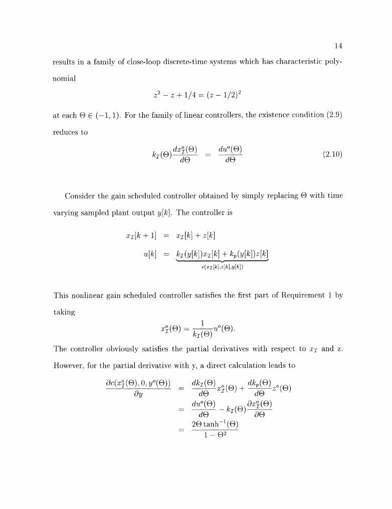
results in a family of close-loop discrete-time systems which has characteristic poly-

noirlial

z2 - z + 114 = (z - 112)~

at each O E (-1,l). For the family of linear controllers. the existence condition (2.9)

reduces to

dx; (0) - -

duo (0) kz(@) d@ d O

Consider the gain scheduled controller obtained by simply replacing O with time

varying sampled plant output y [ k ] . The controller is

This nonlinear gain scheduled controller satisfies the first part of Recluiremerlt 1 t)y

The corltroller obviously satisfies the partial derivatives with respect to .I-= and z.

Howev~r, for the partial derivative with y, a direct calculation leads to

ac(x;(0), 0: yo(@)) - -

dk, (0) dk'(0) p(@) + z0 (0) 3~ d 0 d O

- - duo (0) --

ax;(@) d O k'(@) 30

15

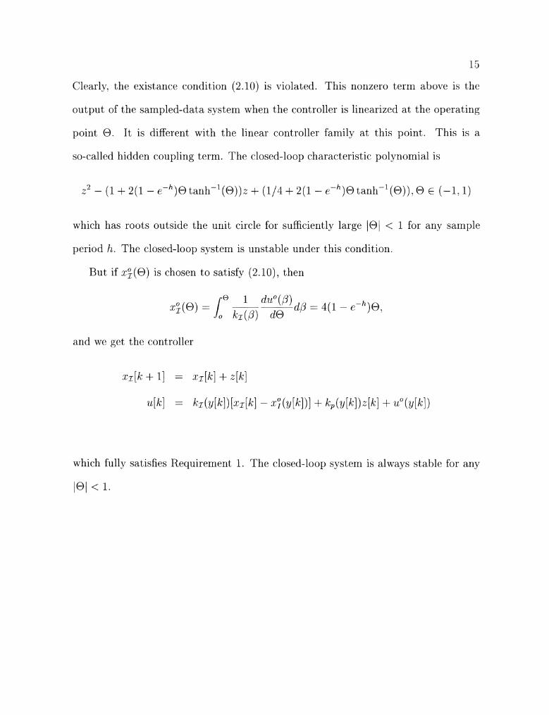
Clearly. the existance condition (2.10) is violated. This nonzero term above is the

output of the sampled-data system when the controller is linearized at the operating

point O . It is different with the linear controller family at this point. This is a

so-called hidden coupling term. The closed-loop characteristic polynomial is

which has roots outside the unit circle for sufficiently large 101 < 1 for any sample

period h. The closed-loop system is unstable under this condition.

But if x ; ( O ) is chosen to satisfy (2.10), then

and we get the controller

x z [ k + 11 = x z [ k ] + z [ k ]

u[k l = ~ z ( Y [ ~ I ) [ ~ z [ ~ I - x ~ ( ~ [ ~ l ) l + ~ , ( ~ ~ k l ) ~ ~ k l + u 0 ( y [ k 1 )

which fully satisfies Requirement 1. The closed-loop system is always stable for any

101 < 1.

Chapter 3

F-16 Aircraft Model

This tliesis applies the gain scheduling rnetl-iod c1cscrik)ed in C1iaptc.r 2 to F-16

aircraft autopilot dcsign. Scctiori 3.1 tlctails t,lic aircraft rrlodcl and rqilations. Sc~.tion

3.2 prciserits thc irriplernentation of an F-16 aircraft sirn~ilat~ion. Socat ion 3.3 lists the

design objec tivcs.

3.1 F-16 Aircraft Mathematical Model

Thc airc:ra,ft aut,opilot is a device wliidi car1 rriairitain or c:harigo t,hc airc:raf% flight,

c:ondit,ions. It, (:an hold aircraft attitiltle, altitudti, aritl flight trajectory by controlling

tlie co~it,rol surface deflectlion of t,hc aircraft and (:rigin(: t,hrust.

Tlie autopilot design in this thcsis irivolves a six-degrcc-of frt:c:tlorn rriodcl of ;in

F-16 aircraft. Tho mat,homa,tical model of tlic F-16 is built in SIMULINK I)asotl on

t,l-le FORTRAN sirnulation in [Ill.

T l ~ o fi)llowi~ig standard 6-DOF(degree of freedorri) equations \vhic:h clc.sc:ril)tr t,licl

<Iyna~nics of t,hc F-16 aircraft tirider a flat-Earth assumption. The dcrivatiori of thci

aircraft ecl~iations is t,hc vector forrn of NewtJon's sccond law of motion. The wiritl

velocity caornponents arc :issurned to bc zero, i.c. a st,ationary air mass.

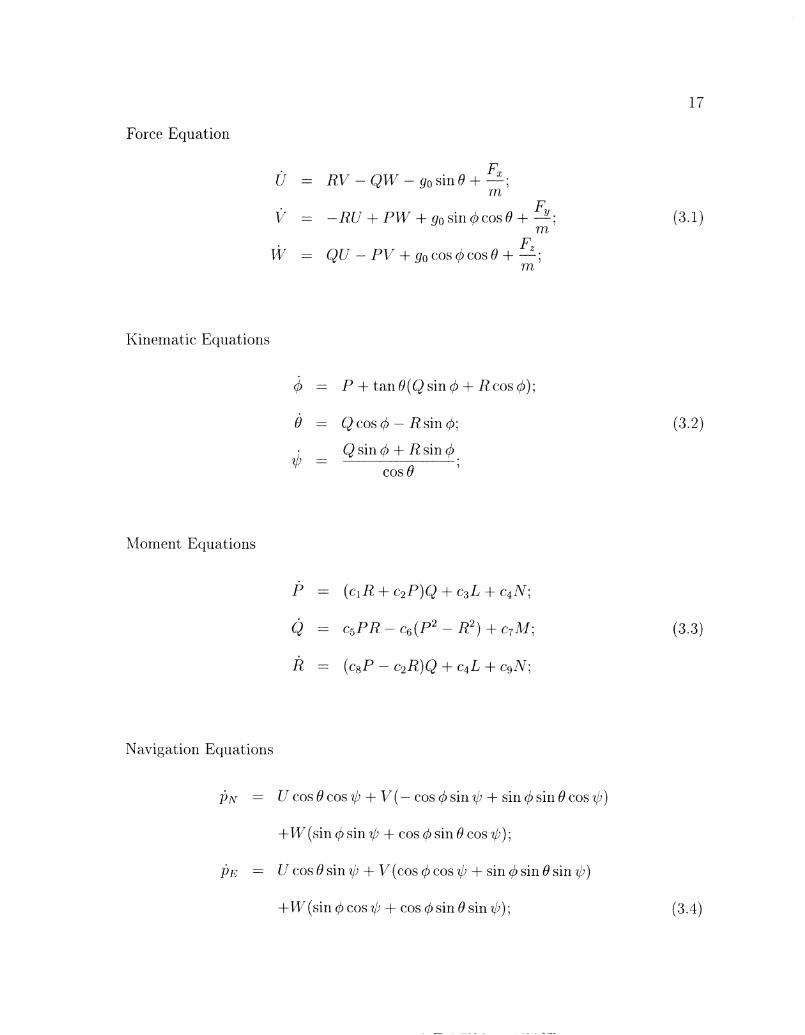
Force Equation

Kinematic Eqtiatiorls

= Q sin 4 + R sin q5

cos 8 >

Moment Equations

Navigation Equations

p~ = U ~ o ~ @ c o ~ I j l + V ( - ~ o ~ q 5 s i n ~ ~ ~ + s i n ~ s i r ~ 0 c o s $ )

+ W (sin $ sin y!i + cos 4 sin 0 cos (4);

I j , = UcosOsin$ + V(cosq5cos$ +s in$s inQs inq)

+ W (sin $ cos $ + cos 4 sin 8 sin $) ;

11 = U sir1 0 - I/'siri 4 cos 0 - W cos 4 cos H ;

The clements of the state vect,or c-:omprise t,he components of the Velocit,y Vector U,

and W ( f t / s ) , t,he V(\ct,or of Eulcr Angles 4 ,Q and $(racrl), the Angular Rate Vector

P, Q and R ( ~ a d / s ) , and the Position Vector p ~ , p ~ . : and h,( f t ) , where, in particula,r, 11,

is altit,~ide. Tlie earth's gravitional accclerat,iori is go = 32.17 f t ls" and t,lic c:onst,;tiits

ci are given by: cl = -0.77, c2 = 0.02755, c:3 = 1.055 x 1 0 ~ " (4 = 1.642 x 10-",

c5 = 0.9604, c6 = 1.759 x c7 = 1.972 x 1 V 5 , cx = -0.7336 and c:, = 1.587 x 1 0 ~ " .

Tlie force vcctor F,, F, arid F,(lbs) and moment vect,or L, M arid N ( b h f t ) rriust he

broken into aerodynamic and thrust contributions provided in [ I l l .

The! aerodynamic forces and rrioments on tlie aircraft depend on the angle of t~ t , t t l~k

and sideslip angle. Also the tnlo :iirspeed lias an effcct on forces and rriorrient,~. It,

is convenient for 11s to use the true airspeed T/ ; ( . f t l s ) , angle of attack tu(rc~,d), arid

sideslipe angle P(7,(1,$) to replace the three velocity vector cornponent,s. The new

stat,e derivatives car1 be derived a,s:

Therefore, we have the state vecator X' = [&, 0, p, 4 , 0 , $, P, &, R , I ) ~ , O ~ , 1 1 1 .

A nurnber of the aerodynamic forccl and rnoriierit componc~nts depend on tho (.on-

trol surface dcflclct,ions, these arct control inputs to t,hc aircraft rriodel. Tlirot,tlc setting

is another control input. The control variables are

vT = [th,, e l , a,il, rud]

where the elements of the vector are, respectively. throttle setting, elevator deflection,

aileron deflection. and rudder deflection.

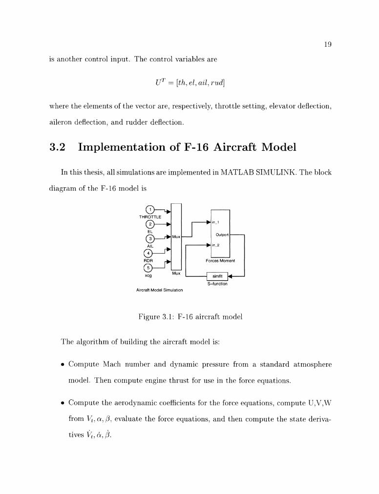
3.2 Implementation of F-16 Aircraft Model

In this thesis, all simulations are implemerited in T\IL4TLAB SIMLLINK. The block

diagram of t,he F-16 model is

THROTTLE 3 AIL

RDR

xcg Mux

Alrcraft Model Sirnulatlon

outport

Forces Moment

simflt & S-function

Figure 3.1: F-16 aircraft model

The algorithm of building the aircraft model is:

Conlplrte 1lac.h number arid dynamic pressure from a standard atrriosphere

model. Then compute engine thrust for lrsc in the force equations.

Compute the aerodynamic coefficients for the force equations, complite U,17.117

from 11;. (L, 3, evaluate the force equations. and then compute the state deriva-

tives I ;, 6, 3.

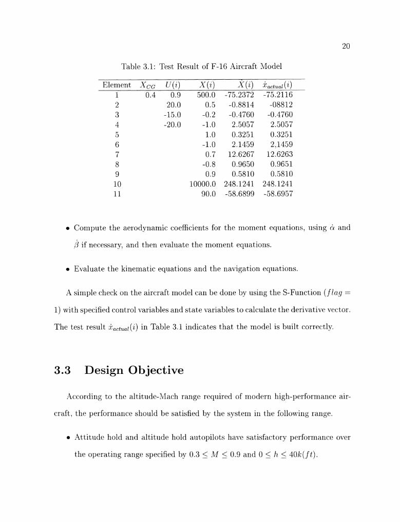
Table 3.1: Test Result of F-16 Aircraft Model

Element XCG U(i) X(i) X(i) xa,t,al ( 2 )

1 0.4 0.9 500.0 -75.2372 -75.2116

Compute the aerodynamic coefficients for the moment equations, using cL and

p if necessary, and then evaluate the moment equations.

Evalliat,e the kinematic equations and the navigation equations.

A simple check on the aircraft model can be done by using the S-Function (f bay =

1) with specified control variables and state variables to calculate the derivative vector.

The test result x~,,~,~,~(z) in Table 3.1 indicates that the model is built correctly.

3.3 Design Objective

According to the altitude-Mach range required of modern high-performance air-

craft, the performance should be satisfied by the system in the following range.

Attitude hold and altitude hold autopilots have satisfactory performance over

the operating range specified by 0.3 < M 0.9 and 0 < h < 40k(ft).

2 1

The glide slope autopilot necds to control thc flight trajectory in air(-raft laricliiig

ovc.r tElc operating range specified by 0.3 < M 5 0.9 ant1 0 5 I r 5 40k ( f t )

a Tho flare c.ontro1 autopilot irilist control tllc aircraft to follow an cxl)onential

trajccbtory frorn alt,it,udc, h less than 30 f t t,o touch tiown.

Chapter 4

F-16 Autopilot Design With Gain Scheduling Technique

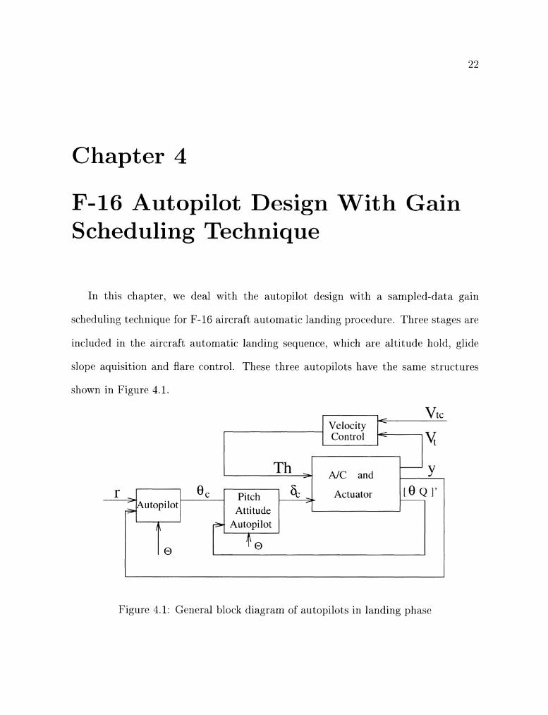
111 this chapter. we deal with thc autopilot design with a sampled-data gain

scheduling technique for F-16 aircraft automatic landing procedure. Three stages arc

included in the aircraft automatic landing sequence, which are altitude hold. glide

slope aquisit ion and flare control. These thrcc autopilots have the same structures

shown in Figure 4.1.

- Th A/C and

- vtc

I I

Figure 4.1: General block diagram of autopilots in landing phase

Velocity Control

< -c IY

23

The velocity controller is designed to control the airspeed, 1; at a specified constant

I i,, and the pitch attitude hold autopilot in the inner loop is constructed to providc

stability augmentation. Here O is the scheduling variable, r represents the c.omrnand

altitude for altitude hold and flare control or the command flight path angle for

glide slope aquisition, y represents the measurement output of altitude for altitude

hold autopilot. of flight path angle for glide slope aquisition, and of altitude and the

derivative of the altitude for flare control.

Section 4.1 gives the calculation of constant operating points and aircraft model

linearization. Section 4.2 presents linear autopilot design for specified operating

points. Section 4.3 details the nonlinear autopilot design with gain schedulirig tech-

nique. Section 4.4 compares the simulation results between the linear autopilot and

the nonlinear autopilot.

4.1 Constant Operating Points and Aircraft Lin- earizat ion

-According to the gain scheduling methodology, the first step of nonlinear gain

scheduled controller design is to cornpute the family of constant operating points

for specificd steady-state flight conditions and linearize the nonlinear aircraft model

a l~ou t the specified flight condition. The operating points of the F-16 are dt>termined

by solving the nonlinear state equations given in Chapter 3 for the state and con-

trol variables to make the state derivatives ?;,&. 3, $, 0, y and P, &, R identicallv

zero. The hank angle d and the sideslip angle f l arc set to be zero. T\I.ATLAAB TRILI

furlction is used to calculate the values of state and control input for given altitudt).

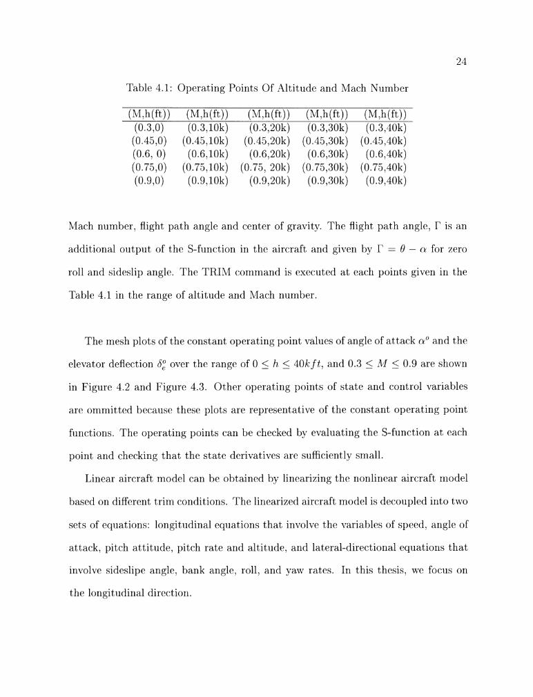
Table 4.1: Operating Points Of Altitude and l lach Number

LIacll number. flight path angle and center of gravity. The flight path angle, r is an

additional output of the S-function in the aircraft and given by r = 0 - CL for zero

roll and sideslip angle. The TRIhl command is executed at each points given in the

Table 4.1 in the range of altitude arid Llach number.

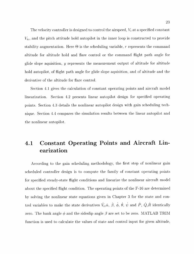
The mesh plots of the constant operating point values of angle of attack o" and the

elevator deflection SP over the range of 0 < iz 5 40k f t , and 0.3 < 141 5 0.9 are shorvn

in Figure 4.2 and Figure 4.3. Other operating points of state and control variables

are omrnitted because these plots are representative of the constant operating point

functions. The operating points can be checked by evaluating the S-function a t each

point and checking that the state derivatives are sufficientlv small.

Linear aircraft model can be obtained by linearizing the nonlinear aircraft model

based 011 different trim conditions. The linearized aircraft model is decouplecl into tn70

sets of equations: longitudinal equations that involve the variables of speed. angle of'

attack. pitch attitude, pitch rate and altitude. and lateral-directional equations that

in\-olve sideslipe angle. bank angle, roll. and yaw rates. In this thesis, rvc focus on

the longitudinal direction.

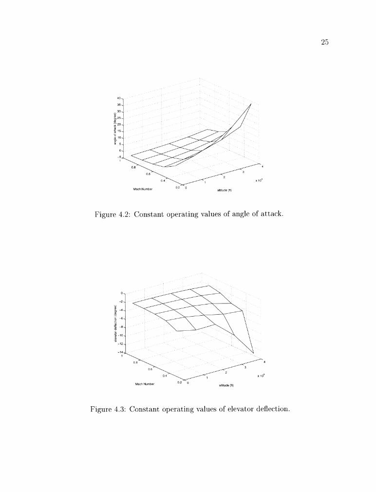
Figure 4.2: Constant operating val~les of angle of attack

Figure 4.3: Constant operating values of elevator deflection.

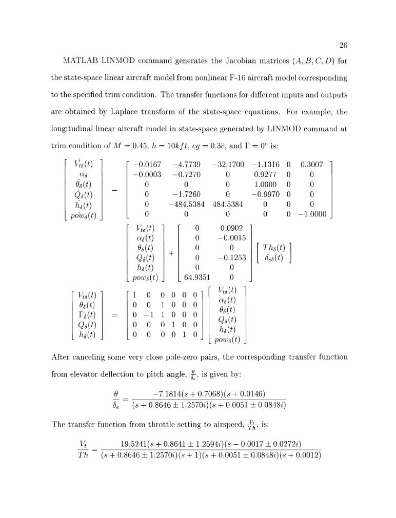
LIATLAB LISMOD command generates the Jacobian matrices (A. B. C. D) for

the statc-space linear aircraft model from nonlinear F-16 aircraft model c-orresponding

to the specified trim condition. The transfer functions for different inputs and outplits

are obtained by Laplace transform of the state-space equations. For example, the

longitudinal linear aircraft model in state-space generated by LINhIOD command at

trim condition of A4 = 0.45, h = l ok f t , cg = 0.3E, and r = 0" is:

rlfter canceling some very close pole-zero pairs, the corresponding transfcr function

frorn clcvator deflection to pitch angle. E, is given by:

The transfer function from t'hrottle set'ting to airspeed, 2; is:

2 7

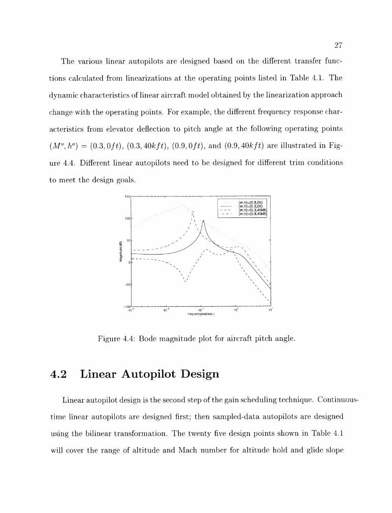
The various linear autopilots are designed based on the different transfer fun(.-

tions calculated from linearizations a t the operating points listed in Table 4.1. The

c-lynamic characteristics of linear aircraft model obtained by the linearization a11proac.h

change with the operating points. For example, the different frequencj, responscl chdr-

acteristics from elevator deflection to pitch angle at the following operatilig points

h") = (0.3. Oft), (0.3.40k f t ) , (0.9. Oft) . and (0.9.40k f t ) are illustrated in Fig-

ure 4.4 Different linear autopilots need t o be designed for different trim conditions

to meet the design goals.

Figure 4.4: Bode magnitude plot for aircraft pitch angle.

4.2 Linear Autopilot Design

Linear autopilot design is the second step of the gain scheduling technique. Continuous-

time linear autopilots are designed first; then sampled-data autopilots are designed

using the bilinear transformation. The twenty fivc design points shown in Table 4.1

will cover the range of altitude and AIach number for altitude hold and glidc slopcl

28

autopilots. The flare control autopilot designed via linearization approach has a satis-

factory perforrrlance for the range of the flare phase, one linear flare control autopilot

is designed for the landing sequence.

4.2.1 Continuous-Time Linear Autopilot Design

Figure 4.1 sho~vs that the velocity controller and pitch att i tude hold controller arp

involved in each phase of landing sequence. They are designed as follows.

Pitch Attitude Hold Autopilot and Velocity Controller

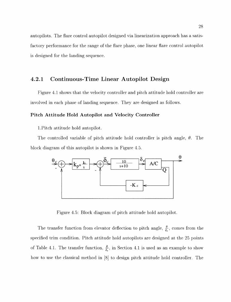
1.Pitch att i tude hold autopilot.

The controlled variable of pitch att i tude hold controller is pitch anglc. 0. Thc

block diagram of this autopilot is shown in Figurc 1.5.

Figure 4.5: Block diagram of pitch att,itude hold autopilot.

The transfer function from elevator deflection to pitch angle, %. comcs fronr thv

specified trim condition. Pitch attitude hold autopilots are designed at the 23 point>s

of Table 4.1. T h r transfer fnnction, $. in Section 4.1 is used as an example to show

how to use the classical method in [8] to design pitch attitude hold controller. The

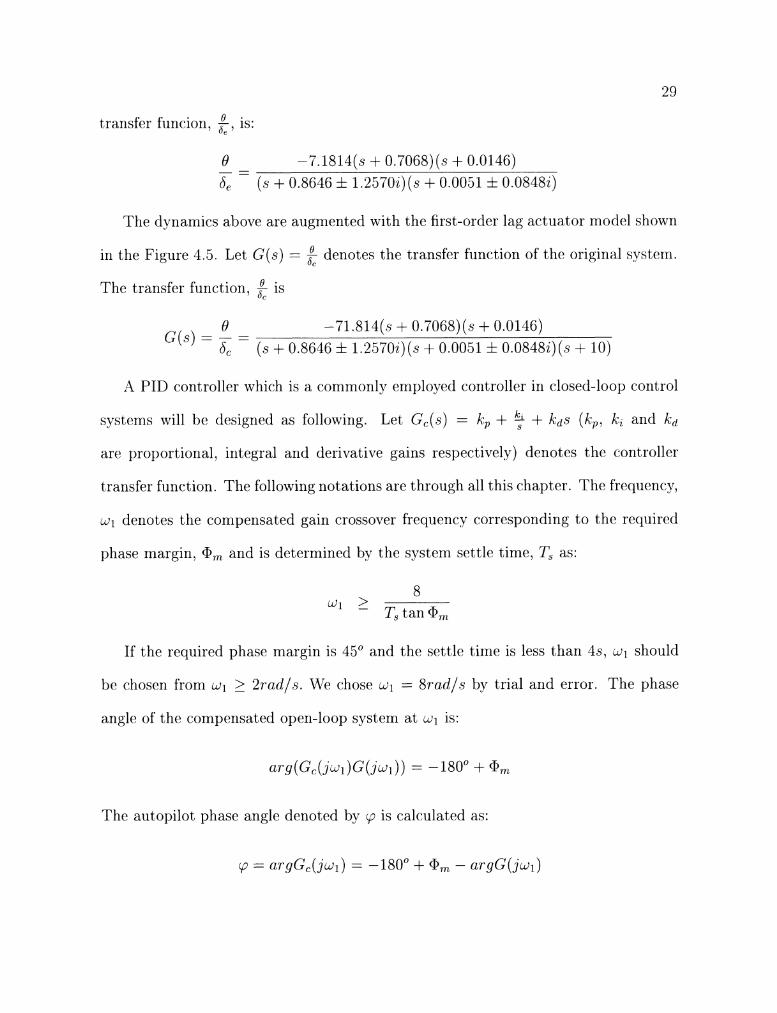
e . transfer funcion, dp, is:

The dynamics above are augmented with the first-order lag actuator rriodel shown

in the Figure 4.5. Let G ( s ) = denotes the trarisfer function of the original system.

The transfer function, is

,-\ PID corltroller which is a commonly employed controller in closed-loop control

systems mill be designed as following. Let G,(s) = k, + $ + k d s (k,. h, auri k,,

are proportional, integral and derivative gains respectively) denotes the (.ontroller

trarisfer function. The following notations are through all this chapter. Thc frequency.

denotes the compensated gain crossover frequencv corresponding to the required

phase margin. @,,, and is determined by the system settle time. Ts as:

8 dl 2 T, tan @,

If the required phase margin is 45" and the settle time is less than 4.5. dl should

be chosen from wl > 2radls . 65'e chose = 8radls by trial and error. The phase

angle of the compensated open-loop system a t dl is:

Thc autopilot phase angle denoted by y is calclilated as:

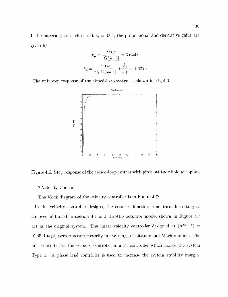
If the integral gain is chosen a t k , = 0.01. the proportional and derivative gains are

given by: cos $5 " = ,G( jd1) ,

= 3.6448

The unit step response of t8he closed-loop systern is shown in Fig.4.6.

Figure 4.6: Step response of the closed-loop systern with pitch att i tude hold aut,opilot'.

Step Response

2.1Telocity Control

0 7 -

$

$ 0 5 -

Q

0 4 -

0 3 +

0 2 -

0 1 .

0 -

The block diagram of the velocity controller is in Figure 4.7:

In the velocit,y controller designs. the transfer function from throttle setting to

T~me (sec I

ii[-:

airspeed obtained in section 4.1 and throttle actuator model shown in Figure 3.7

1 I

0 2 4 6 8 I 0 12 14 16 18

act as the original system. The linear velocity controller designed a t (,If0. 17" ) =

20

(0.35. l 0 k f t ) performs satisfactorily in the range of altitucle and Alach number. Thc

first controller in the velocity controller is a PI controller which makes the systerrl

Type 1. ,Aphase lead controller is used to increase the system stability margin.

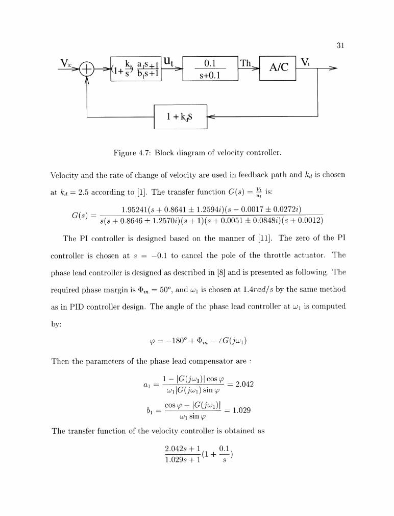
Figure 4.7: Block diagram of velocity controller.

Lelocity arid the rate of change of velocity are used in feedback path a r ~ d k,, is chosen

a t k,! = 2.5 according to [I]. The transfer function G(s) = 2 is:

The P I corlt'roller is designed based on the manner of [ll]. The zero of t,hc P I

corit~roller is chosen at s = -0.1 to cancel the pole of the throttle actuat,or. The

phase lead controller is designed as described in [8] and is presented as following. The

required phase rnargin is a, = SO", and dl is chose11 a t 1 .4rad l s by thc sarne rnetho(1

as in PID controller design. The angle of the phase lead controller a t dl is computed

by:

9 = -180" + cP, - i G ( ~ d 1 )

Then thc parameters of the phase lead compensator are

1 - lG(jwl) 1 cos p a1 = = 2.042

wl lG(jwl) sin q

wl sin q

The transfer function of the velocity controller is obtained as

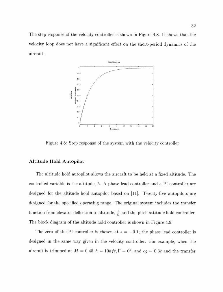
The step rrsponse of the velocity corltroller is shown in Figure 4.8. It shows that the

velocity loop does not have a significant effect on the short-period dynamics of the

aircraft.

Step Response

Figurc 4.8: Step response of the system with the velocity controller

Altitude Hold Autopilot

Thc altitude hold autopilot allows the aircraft to be held a t a fixed altitiide. The

controlled variable is the altitude, h. IZ phase lead controller and a PI controllcr are

designed for the altitude hold autopilot based on [ll]. Twenty-five autopilots arc?

designed for the specified operating range. The original system iricludes thc transfer

fiinction from elevator deflection to altitude. & and the pitch att i tude hold controller.

The block diagram of the altitude hold controller is shown in Figure 4.9:

The zero of the PI controller is chosen a t s = -0.1: the phase lead controller is

designed in the same way given in the velocity controller. For examplc, when the

aircraft is trimmed at LII = 0.43, h = l 0 k f t . r = 0". and cg = 0.37 and thc transfer

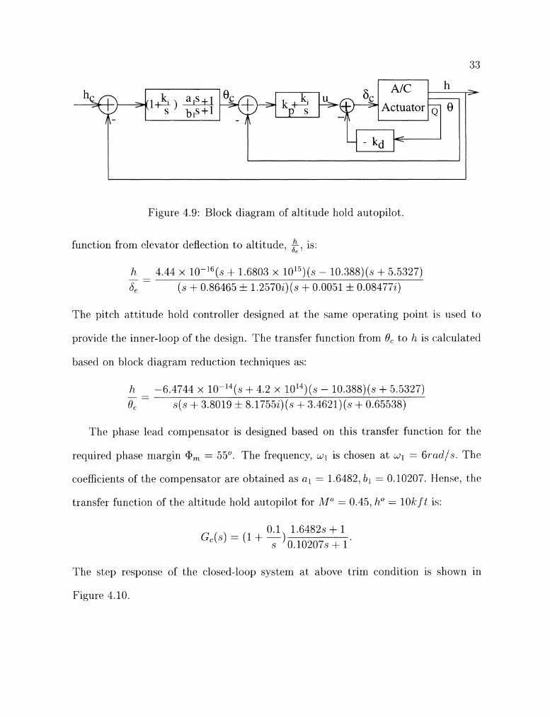
Figure 4.9: Block diagram of altit'ude hold aut'opilot.

A/C

Actuator

function from elevator deflection to altitude. 2. is:

h >

5 0

The pitch att i tude hold controller designed a t the same operating point is used to

provide the inner-loop of the design. The transfer function from 19, t o h is calculated

based on block diagram reduction techniques as:

The phase lead compensator is designed based on this transfer function for the

required phase margin Q, = 55". The frequency. i~ chosen a t = G r n d l i . Thc

corfficierrts of the cornpensator are obtained as a1 = 1.6482. bl = 0.10207. Hen\?, thv

transfer function of the altitude hold autopilot for = 0.45. hO = l0k j t is:

The step response of the closed-loop system a t above trirn conditiori is shown in

Figure 4.10.

Step Response

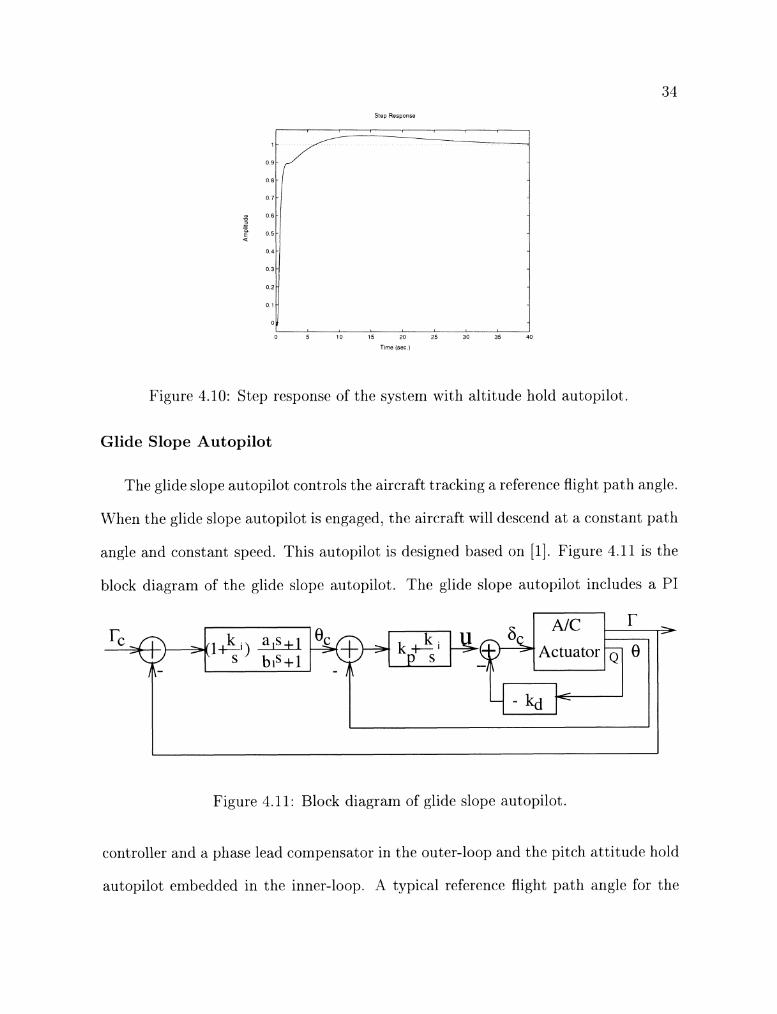
Figure 4.10: Step response of the system with altitude hold autopilot.

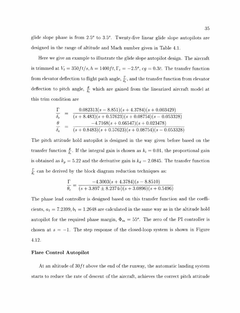
Glide Slope Autopilot

The glide slope autopilot controls the aircraft tracking a reference flight path angle.

When the glide slope autopilot is engaged, the aircraft will descend at a constant path

angle and constant speed. This autopilot is designed based on [I]. Figure 4.11 is the

block diagram of the glide slope autopilot. The glide slope autopilot includes a PI

Figure 4.11: Block diagram of glide slope autopilot.

A/C I-

controller and a phase lead compensator in the outer-loop and the pitch attitude hold

autopilot embedded in the inner-loop. A typical reference flight path angle for the

ec Actuator Q 0 , k . a , s + l (Its') +I

3 5

glide slope phase is from 2.5" t o 3.5". Twenty-five linear glide slope autopilots are

designed in the range of altitude and Mach number given in Table 4.1.

Here we give an example to illustrate the glide slope autopilot design. The aircraft

is trimmed a t 1; = 350 f t l s . h = 1400 f t , I', = -2.5", cg = 0.3T. The transfer fiinctiori

from elevator deflection t o flight path angle, E. and the transfer function from cle\,atur

deflection to pitch angle, $ which are gained from the linearized aircraft rnoclcl at

this trim condition are

The pitch attitude hold autopilot is designed in the nray given before based on the

transfer function 9. If the integral gain is chose11 as k , = 0.01, the proportional gain

is obtained as k , = 5.22 and the derivative gain is kd = 2.0845. The transfer filnctiorl

can be derived by the block diagrani reduction techniques as:

The phase lead controller is designed based on this transfer function arid tho roeffi-

cients. a l = 7.2399, bl = 1.2648 are calculated in the same way as in the altitude hold

autopilot for the required phase margin. a, = 55". The zero of the PI controller is

choscn at s = -1. The step response of the closed-loop system is shown in Figure

4.12.

Flare Control Autopilot

At an altitude of 30 f t above the end of the runway, the automatic landing system

starts to reduce the rate of descent of the aircraft. achieves the correct pitch att i tude

Step Response

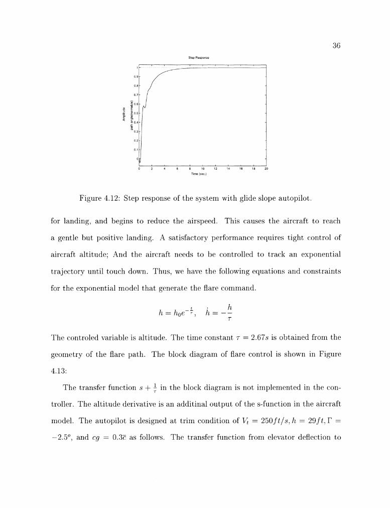
Figure 4.12: Step response of the system with glide slope autopilot.

for landing. and begins to reduce the airspeed. This causes the aircraft to reach

a gentle hut positive landing. -4 satisfactory performance requires tight cont,rol of

aircraft altitude: A4nd the aircraft needs t o be controlled t o track an exponential

trajectory until touch down. Thus, we have the following equations and constraints

for the exponential model that generate the flare command.

The coritroled variable is altitude. The time constant T = 2.67s is obtained from the

geornctry of the flare path. The block diagram of flare control is showri in Figure

The t,ransfcr function s + in the block diagram is not implement,ed in the con-

troller. The altitude derivative is an additinal output of the s-function in the aircraft

model. The autopilot is designed a t trim conditiori of 1; = 250 f t / s , h = 29 f t . r =

-2.5'. and cg = 0.3? as follonrs. The transfer function from elevator deflection to

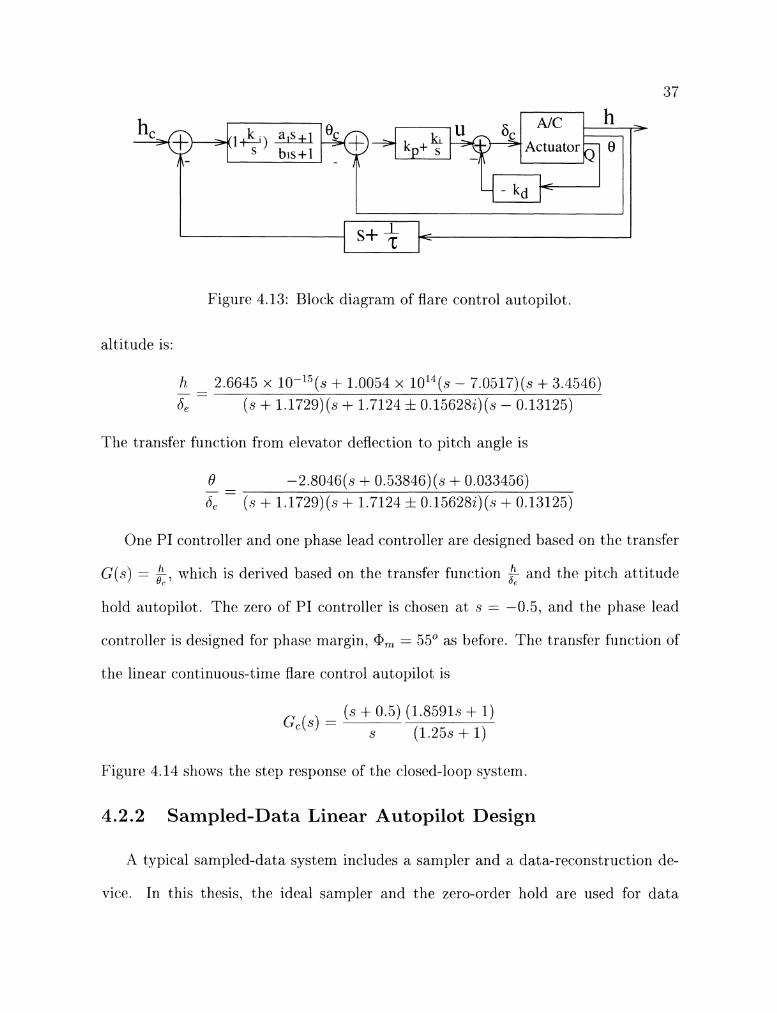
Figure 4.13: Block diagram of flare control aut'opilot.

AIC . h , Actuator - 8

alt.itude is:

-

The transfer funct,iorl from elevator deflection t'o pitch angle is

One P I controller and one phase lead controller are designed based on the transfcr

G ( s ) = k. which is derived based on the transfer function and the pitch attitude

hold autopilot. The zero of PI controller is chosen at s = -0.5. and the phase lead

P

s+ +

coritroller is designed for phase ma,rgin, a,, = 55* as before. The t'ransfer function of

<

the linear continuous-time flare control autopilot is

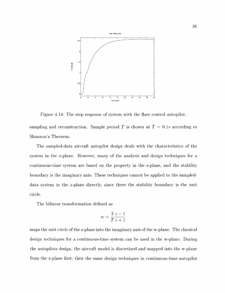
Figure 4.14 shoivs the step response of the closed-loop system.

4.2.2 Sampled-Data Linear Autopilot Design

.A typical sampled-data system includes a sampler and a dat'a-reconstnlct,ion de-

vice. In this thesis. the ideal sampler and the zero-order hold are used for data

Step Response

T~rne (ssc )

Figure 4.14: The step response of systc1rn wit11 tllc flare control al~topilot.

satnpling and rc~constr~iction. Sample periotl T is chosen a t T = 0 . 1 . 5 acc.ortlitig to

Shannori's Thcortlrn.

The satnpled-data aircraft autopilot design dt3als with the c1iaractcristic.s of' tht.

system in tkic. z-planc. Howcvcr, marly of the analysis and design tec.hnicllies for a

continuol~s-time system are based on the property in the s-plane, ancl thc stalility

bo~lndary is thc. imaginary axis. These tt>c.hniquos caririot bc applied to the) sarnpletl-

data systerri in thc z-plane directly, sirice there the stability bountlarv is tho ilrlit

(.it r1e.

The. 1)ilincar tr itnsforrriatiori tlefinetl as

Iriaps t110 unit circ.lc. of the z-plan(. into thc imaginary axis of thc w-plan(.. Thc' c.lassic.al

tlesign tec*hnicli~es for a continuoils-tin1 systcrr~ can he i~sed in the w-plane. During

the autopilots dc~sigri, the. aircraft nlodc\l is discrctized and mapped into thc w-planc

from the z-plane first; then the sarrlc tiesign tec.hniques in contiriuous-tirric autopilot

3 9

dcsign are ~isod to tlesign the pitcbh at titude hold, glide path aqliisition, altit lid(> hold

and flare control autopilots; firralv the autopilots arc. mapped into the z-planc by t hr

t~ilinc~iir trar1sfi)rrnation.

Sa~~ll>led-tlati~ pitch attitude hold, altitildc hold, and glidc slopc autopilot havc1

the sarnr strncturc as in contini~ous-tirrie. Tho flare control has an addit,ion;~l phase

lag ( . o m p ( . ~ ~ ~ i ~ t o ~ to filtcr the high frecluency noise brought by sampling i l ~ ~ t l data-

rec~or~strnctiori [8]. Tho phast> lcad controller arid PID coritrollrr in the w-~>laric> ar (>

designt.d iri the same way as in the s-planc. The frequency, w,,,,, at whirh thc phxscl

rnargin oc.c.111~ in the w-plane rc.lat,cs to thcl frc.cyucncy, wl in s-planc ;is:

All iiut01)ilots in thc w-plane can 1)e rrrapprd into the z-plan(. bv C2DM ( .or r l~~l i~~id .

4.2.3 Example of Simulation with Linear Continuous-Time and Sampled-Data Autopilot

In this section, sorncl sirriulatioir c.x;~mples are given for 1)oth coirtinuons-tirri(1 and

sampled-data alitopilots. The sirriulations arc irnplerrlc~ntcd iri MATLAB SIhlULINK

Thr sarrie trim conditions arc used for both coritinuous-tirnt. and sarnplcd-dilta till-

topilot sirriulation.

The altitild(\ hold autopilot has a similar sirmllation b1oc.k diagrarn with tho gliclt)

slope i~l~topilot , ctxc.ept for thc different controller, input and olltpllt signal, t 21c.1 (.for c',

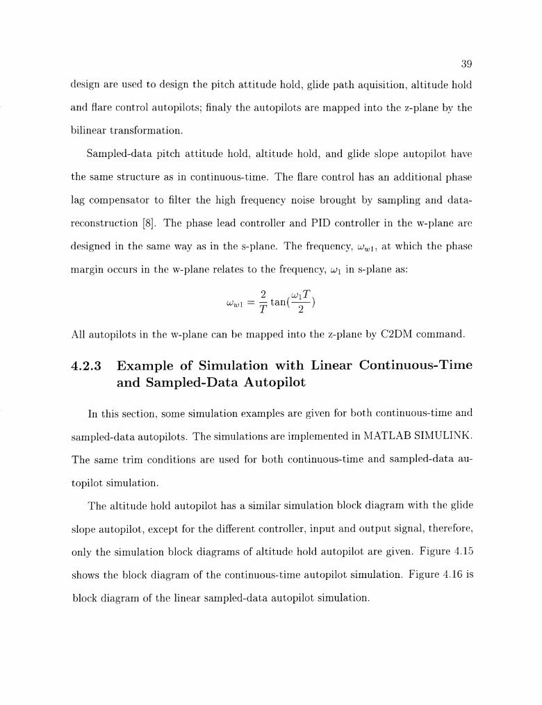
orllv tl-ic sirrilllatioil 1,lock diagriirlls of' altitude holtl autopilot are given. Figure> 3.15

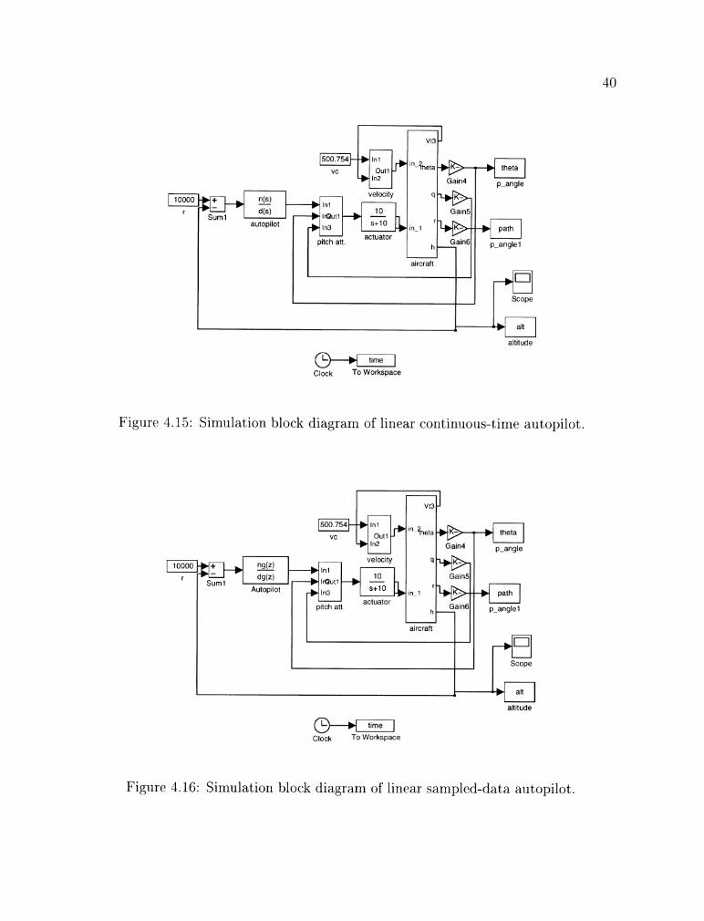
S~-IOWS t h(' block diagrarn of thc cont iriuous-tirricb ;tntopilot sirnulation Figlir c. 3. I G is

block diagrarri of the linear sarnplec-l-data autopilot simulation.

vt3 - 500 754 -+ In1

VC Out1 theta

-+. 1n2 Gain4 p-angle -

altitude

time

clock To Workspace

Figure 4.1.5: Simulation block diagram of linear continuous-time autopilot.

theta

aircraft ' I A Scope I -

alt

altitude

time

clock To Workspace

Figure 4.16: Simulation block diagram of linear sampled-data autopilot.

4 1

Figtirc 4.17 shows the linear simulation result of linear continiloils-tirn(1 altitude

hold autopilot. Figure 4.18 is tlie linear simulatiorl result of the linear sampled-tlata

altitude hold autopilot. The aircraft is trimmed at h = 5000 f t , -21 = 0.45. r = 0"

and cg = 0.37. The simulations show that the sampled-data altitiide hold a l i to~~i lo t

performs as good as the continuous-tinip altitude hold autopilot.

The liriear siniulatiori result of tlie continuous-time glide slope autopilot is shown

in Figlire 1.19. The linear sirnulatiorl rcsiilt of the sampled-data glide slop^ aiito1)ilot

is shown in Figure 4.20. The linear sampled-data glide slopc autopilot has tlie same

sirriulation result as the linear continuous-time glide slope autopilot.

The f l a r ~ ('ontrol autopilot desigried via the linclarization approach covers tlie

r angc of thtl flare control phase for the nonlinc~ar F- 16 air craft. therefore, rionlincar

sirnulatiorl results are presented h ~ r ~ for the flare coiltrol procedurc. Figure 4.21 is tlic

riorilinear simulation result of the continuous-time flare control autopilot. Tho aircraft

is iriitialized at 29 f t altitude, 250 f t l s airspeed. and -2.5" flight path aiiglt.. Figure

4.22 is the noillinear simulatioli result of the sampled-data flare control alltopilot.

From the sirmllation results, the linear sampled-data flare control autopilot llas higger

transie~lt than the continuous-time flare control autopilot. Hornlever, it still s1lon.s

satisfactorv performance.

4.2.4 Family of Linear Autopilot Design

Once li~war autopilots have been designed t o meet the design goals at each 01)-

erating point, thc family of liriear autopilots are coiriputed by ISTERP2 frinctiori to

interpolate the various parameters of the liricar autopilots in the range of altitutle

arid hlach nunil~er.

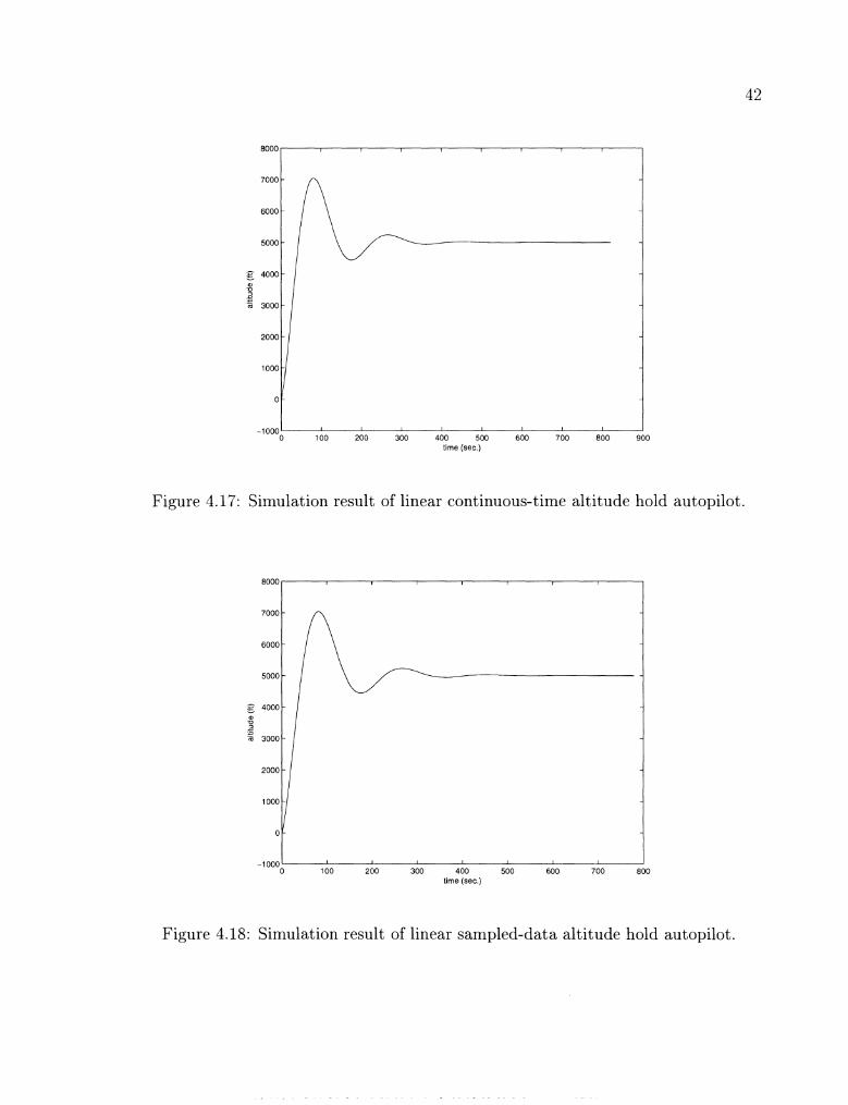
Figure 4.17: Simulation result of linear continuous-time altitude hold autopilot.

-1000- 100 200 I 300 400 500 600 700 800

time (sec.)

Figure 4.18: Simulation result of linear sampled-data altitude hold autopilot.

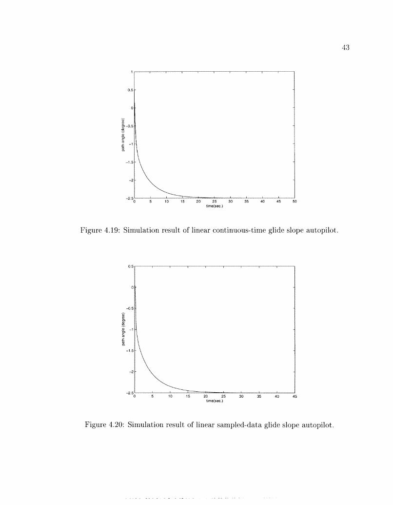
Figure 4.19: Simulation result of linear continuous-time glide slope autopilot.

Figure 4.20: Simulation result of linear sampled-data glide slope autopilot.

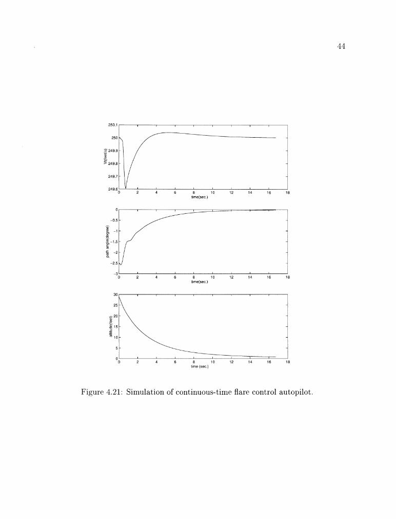
Figure 4.21: Simulation of continuous-t,irne flare control autopilot.

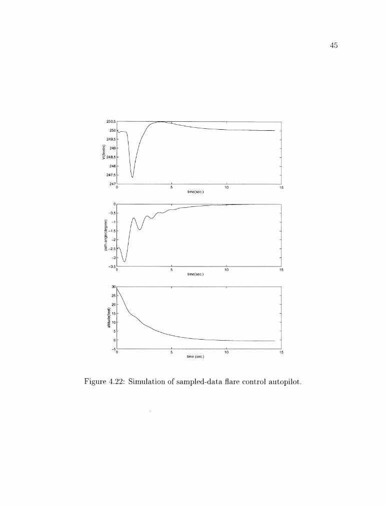
Figure 4.22: Simulation of sampled-data flare control autopilot,.

4.3 Gain Scheduled Autopilot Design

,After the family of linear autopilots are established, n7e can use the methodology

described in Chapter 2 to build the nonlinear gain scheduled autopilots, which are

intended to linearize to the corresponding linear autopilot a t each constant operating

point. Three gain scheduled autopilots will be designed.

4.3.1 Pitch Attitude Hold Autopilot

The nonlinear pitch attitude hold autopilot is contructed based on thc familv of

linear sampled-data pitch attitude hold autopilot designed before. Thc commanded

elevator deflection is the output of the gain scheduled controller. The cornrnarlded

pitch angle is the reference input signal. The regulated variable is the tracking crror

z = 8, - 8. The pitch rate is the additional output of the plant. The farnily of' linear

discrete-time PI controllers has the form

xzd [ k + 11 = xz6 [k] + zg [k] h e , [k] = - k, (O) xzb [k] - k p (0) [k] + kd (O) Qb [k]

where .rZb[k] = xz[k] - xO(0), and zs[k] = 0,[k] - O[k]. The gains k,. k , arid kd arc

furictions of scl-ieduling variable O = [M, h]. The parameterized transfer function

from (2s. (1d) to Seb associated with this state equations is:

47

In a linear systern, it is equivalent to

Defining

it is clear that p O ( 0 ) = 0, ( " ( 0 ) = 0 , and q O ( 0 ) = 0 a t the constant oprrating

point. Therefore, p6[k] = p [ k ] , & [ k ] = < [ k ] , and q 6 [ k ] = ~ [ k ] . Now. consider a linear

sampled-data controller which has form:

.rZd [k + 11 = X Z ~ [ k ] - k , ( 0 ) p 6 [ k ] - k. I-' (@)Cs [ k ] + kd ( @ ) V s [ k ]

se6[k] = X Z J [ ~ ] - k z ( 0 ) p b [ k ] - k p ( 0 ) [ , [ k ] + k d ( ~ ) q 6 [ , + ] (4.3)

The transfer function from ( p 6 , 1 6 , q 6 ) to Se6 is given as

which together with (4 .2 ) has the same transfer function from (26, Q s ) to bps with

(4 .1 ) . The existence condition of a gain scheduled cont'roller sat'isfies Reyuirerrlent 1

given in Chapter 2 is

4 8

which satisfied by taking x7(@) = 6 , " (0 ) . -4 sampled-data gain scheduled controller

that meets Requirement 1 is

4.3.2 Altitude Hold Autopilot

Frorn Section 4.2, altitude, h is the control variable of the linear altitude hold

coritroller. The command altitude, h, is the reference input. Tracking error z = h , - h

is the regulated signal. ,Altitude and Mach number are the scheduling variables. Pitch

anglc and pitch rate are additional system outputs. The controller has three parts.

Inncr-loop PI controller:

Outer-loop PI controller:

2 2 6 [k + 11 = z26 [k ] + ~ [ k ]

u [ k ] = k i ~ 2 6 [ k ] + kPz[k ]

Outer-loop phase lead controller:

x36 [k + 11 = a(O)x36 [ k ] + b(@)u6[k]

Q, [ k ] = ~ ( 0 ) [ k ] + d (O) us [ k ]

where k P l , k d r a, b. c , and d are functions of O = [IW. h] . The family of linear altitude

hold autopilots has the form

~ c d [ k + 11 = All ( O ) x c b [ k ] + -412 ( @ ) ~ ~ b [ k ] + B I O ( 0 ) z S [ k ] + BI I ( @ ) 7 j b [ k ]

J Z ~ [k + 11 = 2x6 [ k ] + z6 [ k ]

be6 [ k ] = CI ( @ ) x c ~ [ k ] + C2 ( @ ) Z Z ~ [ k ] + DO (0) z6 [ k ] + D l (0) yS [ k ]

b (0) k p = [ d ] BIlir: = [ - j j

c, ( O ) = [ -k, , (0) - k t ( @ ) ] . c2(@) = -kpl ( @ ) k i d ( @ )

The transfer function from ( z , y s ) to 6,s is

use the same definitions of p and < as the pitch att i tude hold controller and

define q [ k ] = y [ k ] - y[k - 11. The family of linear discrete-time controllers has the

5 0

forrn

~ o [ k + I ] = 11 ( 0)2c6[k1 + -Al,(O)p6[k] + B l o ( 0 ) [ 6 [ k ] + B,, (@)r16[k]

zn[k + ' I = ' 1 ( @ ) x ~ d [k] + X T J [ ~ ] + C2 ( @ ) p a [k] + Do ( @ ) & [k] + D~ (wljn [ A , ]

aed 1'1 = C1 ( O ) X C ~ [ k ] + 2 1 6 [k . ] + C2 (0) pb [k] + Do (0) t6 [k] + Dl (0) q6 [ k ]

(4.5)

The existence condition of the gain scheduled controller to meet Requirement 1 has

the forrr~

which is satisfied by taking x: (0) = 0 and X $ (0) = 6: ( O ) . Here O [ k ] = O [ k ] . h [ k . ] ) .

gain scheduled controller which meets Requirement 1 is given by

J C [ ~ + 11 = z 4 ~ i ( O [ k ] ) ~ c [ k ] +-412(O[k])p[k] +Blo(O[k] )<[k] + B l l ( O [ k ] ) r , [ k ]

X T [ ~ + I ] = Cl ( O [ k ] ) x c [k] + sz[k-] + C2 ( @ [ k ] ) p [ k ] + DO ( 0 [ k ] ) < [ k ] + Dl (@[k])r l[k]

6, [kI = c, ( @ [ k ] ) x c [k] + .rz[k] + C2 ( @ [ k ] ) p [ k ] + Do ( O [ k ] ) [ [ k ] + D L ( O [ k ] ) ~ 1 [ k ]

(4.6)

4.3.3 Glide Slope Autopilot

The linear glide slope controller has the same structure as the altitude hold con-

troller, except that the reference input is the flight path angle and the regulatetl 5ignal

is 2 = r, - I?. Therefore. the nonlinear gain scheduled controller design is also the

same as the altitude hold controller.

3 1

4.4 Comparison of Simulation Results of Linear Autopilot and Nonlinear Gain Scheduled Au- topilot

In this section. the nonlinear autopilots obtained in Section 4.3 is evaluated bv

sinililatiorl and compared to the linear autopilot for the same trim condition and

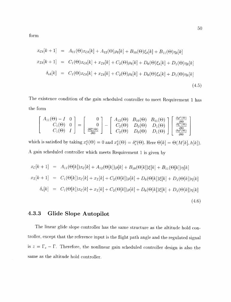
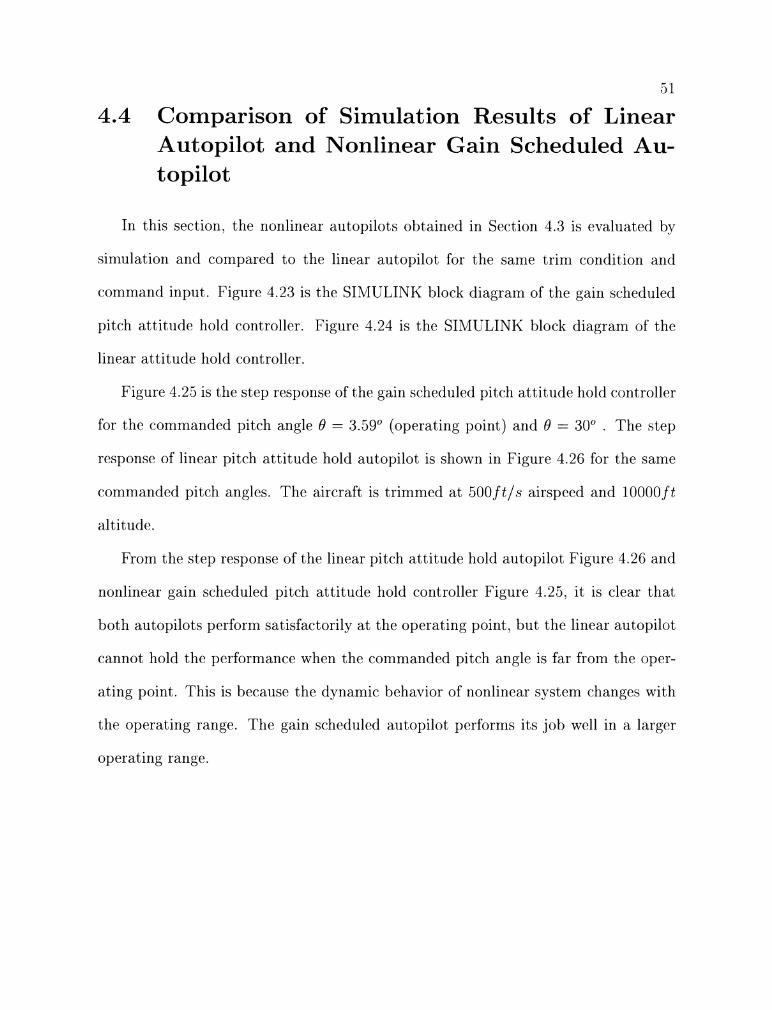
cornmand input. Figure 4.23 is the SILILLINK block diagram of the gairi \c.hedulrtl

pitch attitude hold controller Figure 4.24 is the SI;\~LULINK block diagiarn of the

linear att i tude hold controller.

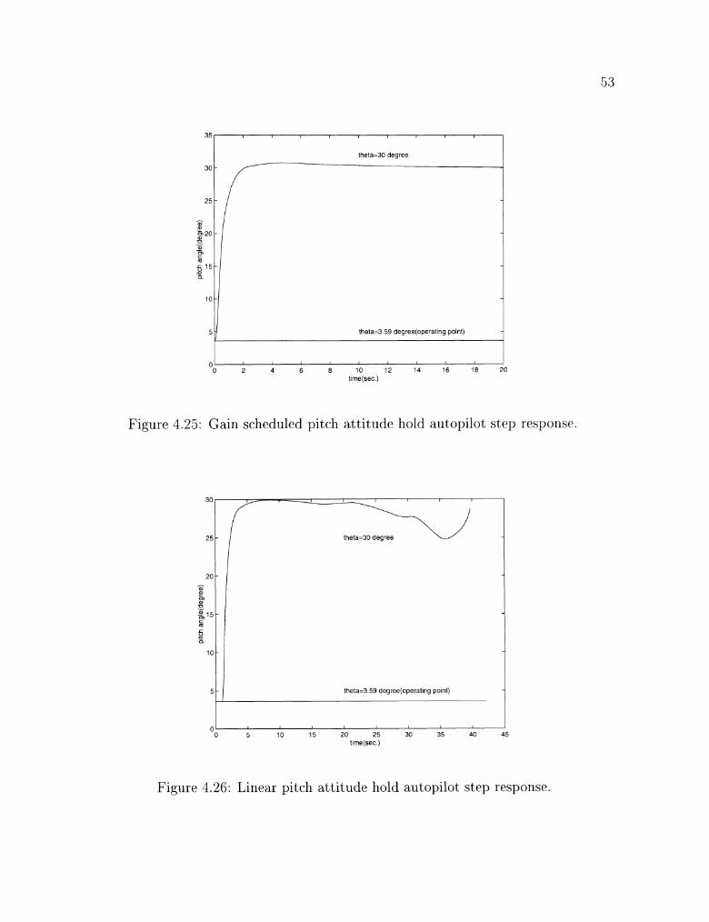
Figure 4.25 is the step response of the gain scheduled pitch att i tude hold controller

for the commanded pitch angle 6' = 3.59' (operating point) and 6' = 30" . Tkic step

response of linear pitch attitude hold autopilot is shown in Figure 4.26 for the sanlc

commanded pitch angles. The aircraft is trimmed at 300 f t / , s airspeed arid 10000 f t

altitude.

From thc stcp response of the linear pitch att i tude hold autopilot Figurc 4.26 and

nonlinear gain scheduled pitch attitude hold controller Figure 4.25, it is clear that

both a~ t~op i lo t s perform satisfactorily a t the operatling point? but the linear autopilot

cannot hold the performance when the commanded pitch angle is far from the oper-

ating point. This is because the dynamic behavior of nonlinear system char~gcs wit11

the operating range. The gain scheduled autopilot performs its job well in a larger

operatirig range.

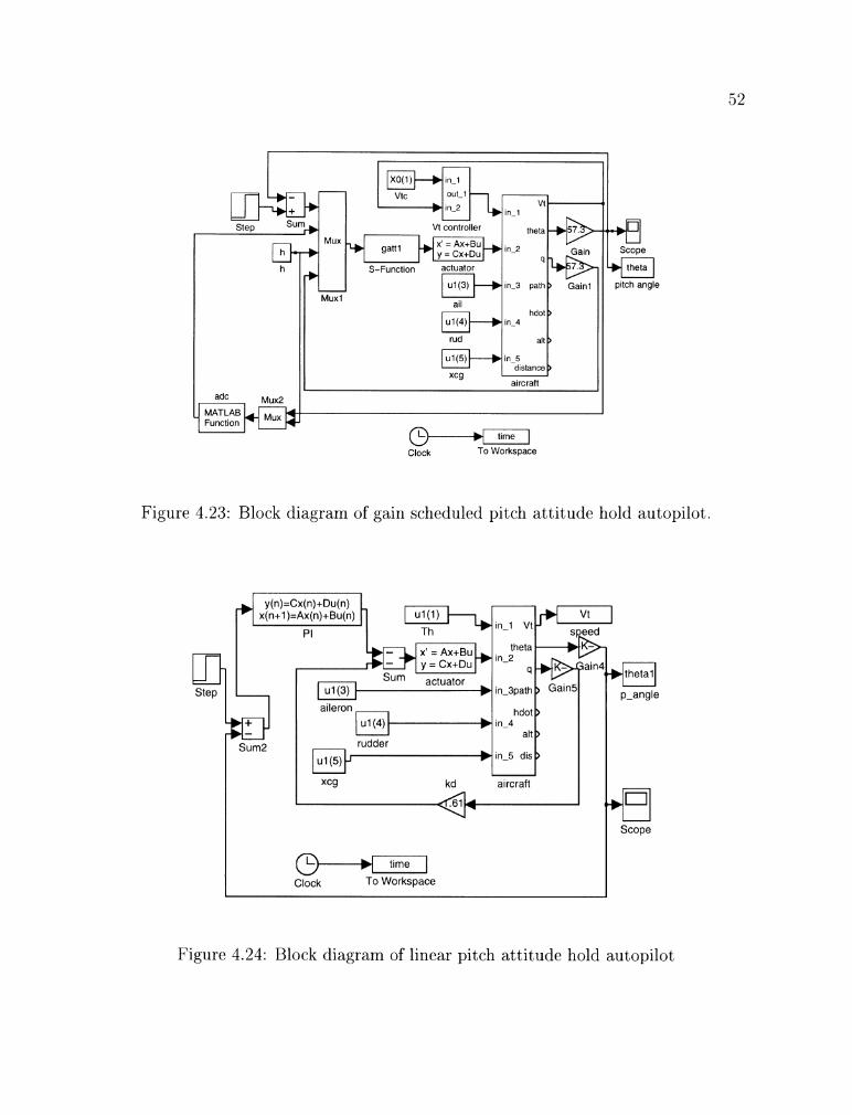
Figure 4.23: Block diagram of gain scheduled pitch attitude hold autopilot

y(n)=Cx(n)+Du(n) x(n+l)=Ax(n)+Bu(n)

PI

( u l (3 ) I P-angle aileron hdot >

a~rcraft

time

Clock To Workspace

- Scope

Figure 4.24: Block diagram of linear pitch attitude hold autopilot

35

thela=30 degree 1

Figure 4.25: Gairi scheduled pitch att i tude hold autopilot step resporiso.

Figure 4.26: Linear pitch attitude hold autopilot step response.

5 1

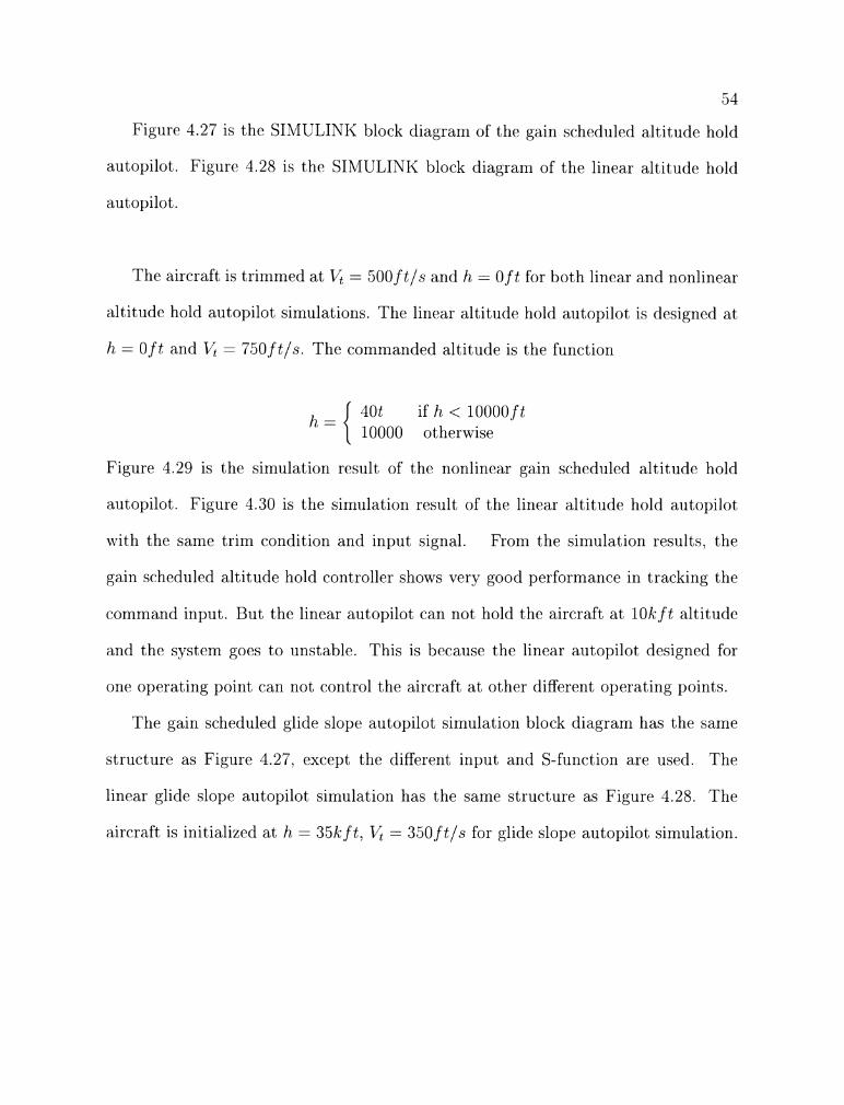
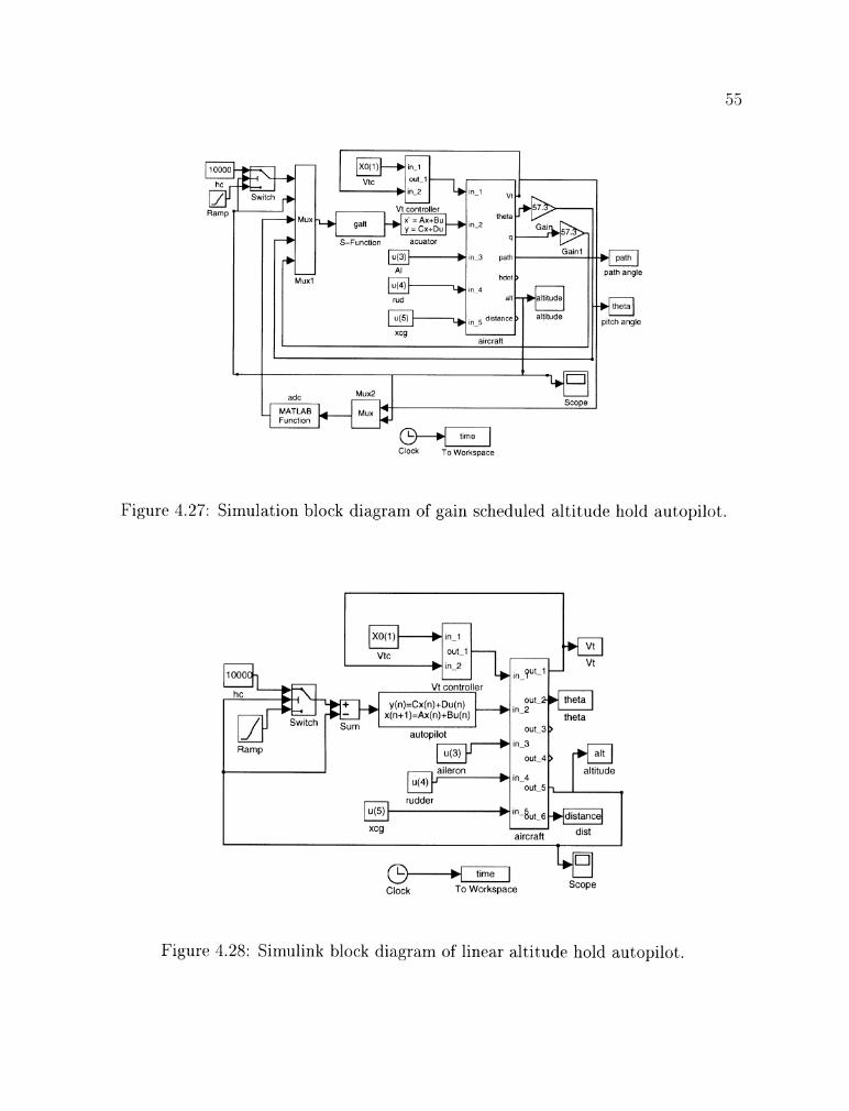
Figure 4.27 is the SILICLINK block diagram of the gain scheduled altitude hold

autopilot. Figure 4.28 is the SIA/IULISK block diagram of the linear altitude hold

autopilot.

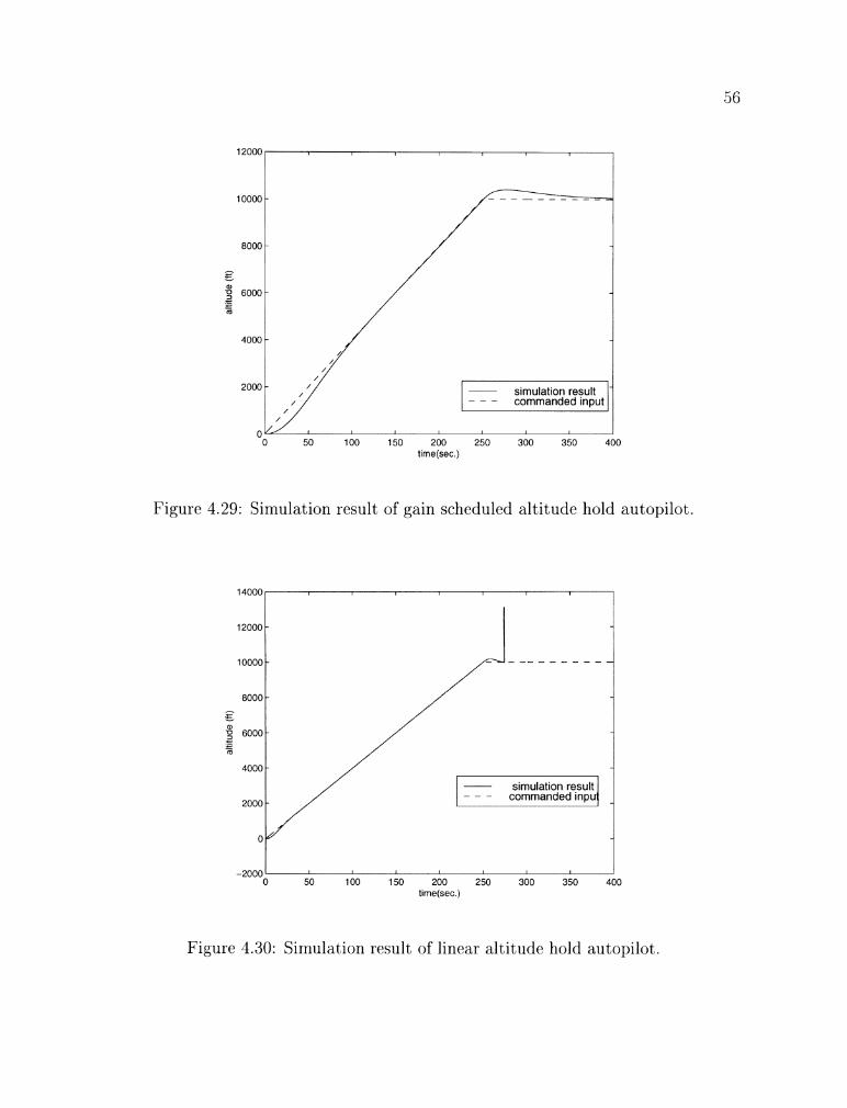
The aircraft is trimmed a t I$ = 500 f t i s and h = 0 f t for both linear and nonlinear

altitude hold autopilot simulations. The linear altitude hold autopilot is dcsigried at

FL = Oft and 1; = 750 f t i s . The commanded altitude is the function

h = { 40t ifh<lOOOOft 10000 otherwise

Figure 4.29 is the simulation result of the nonlinear gain scheduled altitude hold

autopilot. Figure 4.30 is the simulation result of the linear altitude hold autopilot

with the same trim condition and input signal. From the simulation results. the

gain scheduled altitude hold controller shows verv good performance in tracking thc

command input. But the linear autopilot can riot hold the aircraft a t l 0 k f t altitude

and the system goes to unstable. This is because the linear autopilot designed for

onc operating point can not control the aircraft at other different operating points.

The gain scheduled glide slope autopilot simulation block diagram has thc samc

structure as Figure 4.27. except the different input and S-function are usetl. The

linear glide slope autopilot simulation has the same structurc as Figlirc 4.28 The

aircraft is initialized a t h = 35k f t. 1; = 350 f t l s for glide slope autopilot simulation.

Muxl

r ud

a~rcraft

adc

MATIAB Funct~on

Clock To Workspace

Figure 4.27: Simulation block diagram of gain scheduled altitude hold autopilot,.

rudder

xcg

Vtc b

1 I

tlme

Clock To Workspace Scope

Figure 4.28: Simulink block diagram of linear altitude hold autopilot'.

Vt controller

y(n)=Cx(n)+Du(n) x(n+l)=Ax(n)+Bu(n)

autopilot Out-3 >

Ramp ~ n - 3

out-4 > altitude + ln-4

Out-5 -,

~ n - 1

out-1

~2 -

Vt ,n-PUt-l

-

- - - s~mulaf~on result cornmandea Inmr

Figure 4.29: Simulation result of gain scheduled altitude hold aut,opilot.

Figure 4.30: Simulation result of linear altitude hold autopilot,.

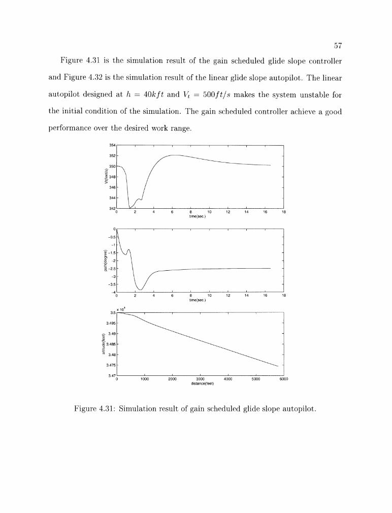
Figure 4.31 is the simulation result of the gain scheduled glide slope cont,roller

and Figure 4.32 is the simulation result of the linear glide slope autopilot. The linear

autopilot designed at 11 = 40k f t and 1; = SO0 f t l s makes the system unstal~le for

the initial condition of the simulation. The gain scheduled controller achieve a gootl

performance over the desired work range.

3.47 1 I 1000 2000 3000 4000 5000 6000

distance(fee1)

Figure 4.31: Simulation result of gain scheduled glide slope autopilot,.

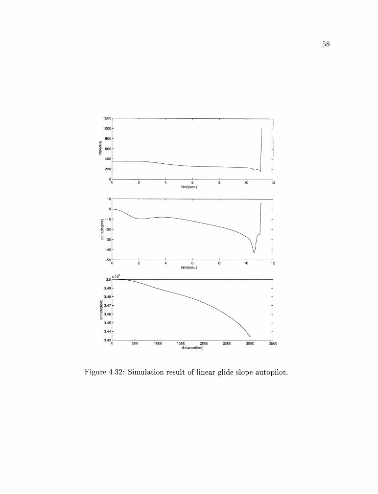
Figure 4.32: Simulation result of linear glide slope autopilot,.

Chapter 5

Conclusions

In this thesis. autopilots for a11 F-16 aircraft n7ere designed using a sarnpled-

data gain scheduling technique. 1Ve introduced the theory and framework of' the

sampled-data gain scheduled technique. \Ve also described the F-16 aircraft dvnarnic

model and gave necessary explanations. The autopilots are designed according to the

procedure listed in Chapter 2. We used SILIULINK to implement the syste~ns and

sirnulate their dynamic performance.

The first step in the gain scheduling technique is to compute the family of constant

operating points and linearize the system a t several equilibrium points. Tlie second

step is to design a family of linear controllers a t each operating point that perforrr~s

satisfactorily when the system is operating near the respective operating points. After

exploring the frequency characteristic of the svstem. we designed several kinds of

controllers to reach the design objective by the classical linear design techniques.

Simulation showed that we achieved satisfactory performance around t he operatirig

points.

Gain scheduling can extend the validity of a controller's operation to a set of'

operating points. JVe designed the sampled-data gain scheduled controller from t h ~

G 0

fanlily of linear controllers. Simulating results show that satisfactory performances

are obtained in the required range.

Since the model used (F-16 aircraft model) is a general model, nrc can corlstruct

the rnodels of many other aircraft in the same structure. The design method we used

ga.i7e a framework for autopilot designs. This approach can also be extended to de.;ign

autopilots for other aircrafts.

For further research work, lateral-direction autopilots for the F-16 aircraft shollltl

11e designed to obtain six degree of freedom autopilots. More modern control dcsigri

techniques will be involved in the full six degree of freedom linear autopilot dcsigr~s.

wind gust model needs to be considered as a perturbation source of the norllincar F-

16 aircraft model. Finally. the experience ive gained from the longitudinal a l i to~~i lo ts

design for the F-16 aircraft will be applied to the autopilot design for the Lrimanned

Aerial l'ehicle project in the Avionics Engineering Center.

Bibliography

[l] Jollrl H. Blakelock. Automatic Control of Aircraft and Missiles. 1Yilf.y

Interscience, 1991.

[2] Isaac Kaminer, Antonio 11. Pascoal. Prarnod P. Khargonekar. and Ed~vard E.

Coleman. A velocity algorithm for the implementation of gain-scheduled con-

trollers. Automatzca, 31 (8):1185-1191, 1995.

[3] Douglas -1 Lawrence. Analysis and design of gain scheduled sampled-data control

systems. Submitted to Automatzca, 1998.

[4] Douglas -1 Lawrence. stability property of nonlinear sampled-data systems

with slonrly varying inputs. In Proceedings of the 1998 Amerzcan Control Cow

ference. pages 2907-291 1, 1998.

[5] Douglas a4. Lawrence, Joy H. Kelly. and Johnny H. Evers. Gain schcdulrd missile

autopilot design using a control signal interpolation technique. In Proc~c(lznc/,s o f

the 1998 AIAA Guzdance, Navzgatzon, and Control Conference, pagcs 98-1 18.

1998.

62

[6] Douglas A. Lawrence and LTTilson J. Rugh. On a stability theorem for norilin~ar

systems with slowly varying inputs. IEEE Transactzons on A1ltornat7c Corrtrol.

35(7).860-864. July 1990.

[7] Douglas A. Lawrence and 'Il'ilson J . Rugh. Gain scheduling dynaniic linear

controllers for a nonlinear plant. Automatzca,. 31 (3):381-390. LIarch 1995.

[8] Charles L . Phillips and Royce D. Harbor. Feedback Control System. P r ~ n t i c e

Hall, 1991.

[9] 11-ilson ,J. Rugh. a4nalytical fi-amework for gain scheduling. IEEE Control Systerrl

Magazzne. 11 : 79-84. 1991.

[lo] Jeff S. Shamnla and hlichael -4thans. Analysis of gain scheduled control for

rionlinear plants. IEEE Tra,nsactaons on Automatzc Control. 35(3):898-907. 1990.

I 111 Brian L. Stevens and Frank L. Lewis. Aircraft Control and Simulation.

1l'illy Interscience, 1992.

[12] David P. \Thite, Jason G. Wozniak. and Douglas -4. Lawrence. Missile. a u t o ~ ~ i l o t

design using a gain scheduling technique. In Proceedzngs o,f thp 26th Soi~theusterrr

Symposzurn on System Theory, pages 606-610, 1994.