ALL SIC TRACTION CONVERTER FOR LIGHT RAIL

ALL SIC TRACTION CONVERTER FOR LIGHT RAIL TRANSPORTATION

SYSTEMS: DESIGN METHODOLOGY AND DEVELOPMENT OF A 500 - 900

VDC, 165 KVA PROTOTYPE

A THESIS SUBMITTED TO

THE GRADUATE SCHOOL OF NATURAL AND APPLIED SCIENCES

OF

MIDDLE EAST TECHNICAL UNIVERSITY

BY

DOĞAN YILDIRIM

IN PARTIAL FULFILLMENT OF THE REQUIREMENTS

FOR

THE DEGREE OF DOCTOR OF PHILOSOPHY

IN

ELECTRICAL AND ELECTRONIC ENGINEERING

SEPTEMBER 2021

Approval of the thesis:

ALL SIC TRACTION CONVERTER FOR LIGHT RAIL

TRANSPORTATION SYSTEMS: DESIGN METHODOLOGY AND

DEVELOPMENT OF A 500 - 900 VDC, 165 KVA PROTOTYPE

submitted by DOĞAN YILDIRIM in partial fulfillment of the requirements for the

degree of Doctor of Philosophy in Electrical and Electronic Engineering, Middle

East Technical University by,

Prof. Dr. Halil Kalıpçılar

Dean, Graduate School of Natural and Applied Sciences

Prof. Dr. İlkay Ulusoy

Head of the Department, Electrical and Electronics Eng.

Prof. Dr. Muammer Ermiş

Supervisor, Electrical and Electronics Eng., METU

Examining Committee Members:

Assist Prof. Dr. Emine Bostancı Özkan

Electrical and Electronics Engineering, METU

Prof. Dr. Muammer Ermiş


Assoc. Prof. Dr. Ozan Keysan


Prof. Dr. Işık Çadırcı

Electrical and Electronics Engineering, Hacettepe University

Prof. Dr. Mehmet Timur Aydemir

Electrical and Electronics Engineering, Kadir Has University

Date: 24.09.2021

iv

I hereby declare that all information in this document has been obtained and

presented in accordance with academic rules and ethical conduct. I also declare

that, as required by these rules and conduct, I have fully cited and referenced

all material and results that are not original to this work.

Name Last name : Doğan Yıldırım

Signature :

v

ABSTRACT

ALL SIC TRACTION CONVERTER FOR LIGHT RAIL

TRANSPORTATION SYSTEMS: DESIGN METHODOLOGY AND

DEVELOPMENT OF A 500 - 900 VDC, 165 KVA PROTOTYPE

Yıldırım, Doğan

Doctor of Philosophy, Electrical and Electronic Engineering

Supervisor : Prof. Dr. Muammer Ermiş

September 2021, 242 pages

Design methodology and development of a 165 kVA, all-silicon carbide (SiC)

traction converter for new generation light rail transportation systems (LRTS) have

been carried out in this thesis. Electrical, mechanical, and thermal design principles

of all-SiC power MOSFET-based traction converter have been described in detail.

In order to verify the produced converter, design and implementation of a full-scale

physical simulator of an all-SiC traction motor drive for LRTS have been performed.

A complete mathematical model of the physical system has been derived to carry out

real-time simulations of LRTS, which takes into consideration the actual two-

quadrant speed versus torque characteristics of a typical traction motor drive. Power

losses and thermal performance of SiC power MOSFET modules have been assessed

in comparison with those of the alternative Hybrid-IGBT and Si-IGBT modules for

various switching frequencies, and their advantages have been considered in view of

converter design objectives. This analysis is also repeated for three-level converter

topologies in order to visualize the effect of SiC power MOSFETs on converter

topology selection. Implementation techniques of the resulting converter power

vi

stage, involving the DC and AC laminated busbars, the general layout, and

associated cooling system, have been paid special attention. The application method

of the space vector PWM technique for operation under variable DC catenary

voltages over a wide range has been uniquely described. The associated experimental

results were taken on the developed all-SiC power MOSFET-based traction inverter

and full-scale physical simulator for LRTS. Very promising results have been

obtained on the track of converter design objectives in terms of performance criteria

such as very high efficiency, low motor line current total demand distortion, low

cooling requirement, relatively high switching frequency, and hence ease of

controller implementation.

Keywords: Railway Traction Inverters, SiC Power MOSFET, Induction Machine

Drive, Field Oriented Control, Space Vector Pulse Width Modulation

vii

ÖZ

HAFİF RAYLI TAŞIMA SİSTEMLERİ İÇİN SIC ÇEKİŞ KONVERTÖRÜ:

TASARIM METODOLOJİSİ VE 500 - 900 VDC, 165 KVA PROTOTİPİNİN

GELİŞTİRİLMESİ

Yıldırım, Doğan

Doktora, Elektrik ve Elektronik Mühendisliği

Tez Yöneticisi: Prof. Dr. Muammer Ermiş

Eylül 2021, 242 sayfa

Bu tezde, yeni nesil hafif raylı ulaşım sistemleri için 165 kVA, tamamı SiC güç

MOSFET’lerinden oluşan bir cer dönüştürücünün tasarım metodolojisi ve

geliştirilmesi gerçekleştirilmiştir. SiC güç MOSFET tabanlı cer konvertörlerinin

elektriksel, mekanik ve termal tasarım prensipleri detaylı olarak anlatılmıştır. Hafif

raylı taşıma sistemleri için geliştirilen tamamı silikon karbür (SiC) tabanlı cer motoru

sürücüsünün testi için tam ölçekli, fiziksel simülatörünün tasarımı ve uygulaması

yapılmıştır. Hafif raylı taşıma sistemlerinin gerçek zamanlı simülasyonlarını

gerçekleştirmek için, fiziksel sistemin eksiksiz bir matematiksel modeli türetilmiştir.

SiC güç MOSFET modüllerinin güç kayıpları ve termal performansı, çeşitli

anahtarlama frekansları için alternatif hibrit ve Si-IGBT modüllerininkilerle

karşılaştırılarak değerlendirilmiş ve dönüştürücü tasarım amaçları açısından

avantajları göz önünde bulundurulmuştur. Bu analiz ayrıca SiC güç MOSFET'lerinin

dönüştürücü topoloji seçimi üzerindeki etkisini görünür kılmak için üç seviyeli

dönüştürücü topolojileri için de tekrarlanmıştır. Konvertör tasarımında, DC ve AC

lamine baralara, genel yerleşime ve soğutma sistemini içeren güç modülü üretimi

için uygulama tekniklerine özel dikkat gösterilmiştir. Geniş bir aralıkta değişken DC

viii

katener voltajları altında çalışma için uzay vektörü PWM tekniğinin uygulama

yöntemi, geliştirilmiş tam ölçekli, SiC güç MOSFET tabanlı çekiş dönüştürücüsünde

ve inşa edilen test düzeneğinde alınan ilgili deneysel sonuçlarla benzersiz bir şekilde

tanımlanmıştır. Çok yüksek verim, düşük motor akımı bozulması, düşük soğutma

gereksinimi, nispeten yüksek anahtarlama frekansı ve dolayısıyla kontol yöntemi

uygulama kolaylığı gibi performans kriterleri açısından yeni teknoloji evirici tasarım

hedeflerinin izinde çok umut verici sonuçlar elde edilmiştir.

Anahtar Kelimeler: Demiryolu Araçları Çekiş Evirgeçleri, SiC Güç MOSFET,

Asenkron Makina, Sürücüsü, Alan Yönlendirmeli Kontrol, Uzay Vektörü Darbe

Genişlik Modülasyonu

ix

To My Family and To My Parents

x

ACKNOWLEDGMENTS

I would like to express my deepest gratitude to my supervisor Prof. Dr. Muammer

Ermiş, for his guidance, advice, criticism, and encouragement.

I would also like to show my gratitude also to Prof. Dr. Işık Çadırcı for her guidance,

advice, criticism, and encouragement.

I would like to thank Assoc. Prof. Dr. Ozan Keysan for his suggestions and

comments in my thesis progress committee.

I would like to thank my friends Hakan Akşit, Behrang Hosseini, Tevfik Pul, and

Cem Yolaçan for their contributions to laboratory tests.

I would like to thank Cezmi Ermiş for his contribution to the mechanical design and

construction works.

I would like to thank TÜBİTAK TEYDEB for its financial support to build

laboratory test setup.

I would like to thank my company ASELSAN, for its financial support to build

laboratory test setup.

I would like to thank my friend Berkan Çakır for his encouragement and continuous

morale support.

Finally, I would like to express my thankfulness to my family and my parents for

their endless patience, encouragement, and continuous morale support.

xi

TABLE OF CONTENTS

ABSTRACT ............................................................................................................... v

ÖZ………………………………………………………………………………… vii

ACKNOWLEDGMENTS ......................................................................................... x

TABLE OF CONTENTS ......................................................................................... xi

LIST OF TABLES ................................................................................................... xv

LIST OF FIGURES .............................................................................................. xvii

LIST OF ABBREVIATIONS ............................................................................. xxvii

CHAPTERS

1 INTRODUCTION .......................................................................................... 1

1.1 History of Railway Vehicles ........................................................................... 1

1.1.1 Types of Railway Traction Systems ............................................................... 3

1.1.2 Types of Railway Electrification Systems ...................................................... 4

1.2 Electric Powered Traction Drives for Railway ............................................... 6

1.3 Today’s Power Converters for Railway Traction Drive ............................... 14

1.4 Power Semiconductors and Development Trends for Railway Traction ...... 18

1.5 Problem Statement and Motivation............................................................... 22

1.6 Scope of the Thesis ....................................................................................... 24

2 LIGHT RAIL TRANSPORTATION SYSTEMS ........................................ 27

2.1 System Architecture ...................................................................................... 28

2.1.1 Functions of Traction System Components .................................................. 30

2.1.2 Types of Railway Vehicles ........................................................................... 37

2.1.3 Physics of Railway Vehicle Motion ............................................................. 39

xii

2.1.4 Power Quality Issues .................................................................................... 48

2.2 Traction Motors used for Railway Traction ................................................. 50

2.2.1 DC Traction Motor ....................................................................................... 51

2.2.2 Induction Motor ............................................................................................ 54

2.2.3 Permanent Magnet Synchronous Motor ....................................................... 57

2.2.4 Comparison of Traction Motors ................................................................... 59

2.3 Topological Overview of Two-Level Voltage Source Traction Inverters ... 61

2.3.1 Operating Principles ..................................................................................... 63

2.3.2 Modulation of Two-level Three-phase Voltage Source Inverter ................. 65

2.4 Topological Overviews of Three-Level Neutral Point Clamp (NPC) and T-

Type Voltage Source Traction Inverters ................................................................. 71

2.4.1 Operating Principles of Three-level NPC and T-Type Voltage Source

Traction Inverters .................................................................................................... 75

2.4.2 Modulation of Three-level NPC and T-type Three-phase Voltage Source

Inverters ................................................................................................................... 77

2.5 Comparative Evaluation of Si-IGBT based Three-Level, and SiC MOSFET

based Two-Level Voltage Source Traction Converters .......................................... 82

2.6 Voltage and Current Waveform Synthesizing .............................................. 85

2.6.1 Pulse Width Modulation Methods ................................................................ 86

2.7 Principles of Electric Traction Drives .......................................................... 98

2.7.1 Control Methods for Voltage Source Inverter Fed Induction Machines in

Railway Applications .............................................................................................. 99

3 DESIGN AND IMPLEMENTATION OF ALL SIC TRACTION

INVERTER ........................................................................................................... 105

3.1 Design Methodology of Prototype System ................................................. 105

xiii

3.2 Requirements of Prototype System ............................................................. 107

3.3 Selection of Power Switches and Switching Frequency ............................. 111

3.3.1 Loss Evaluation for 2L Inverter Topology ................................................. 114

3.3.2 Loss Evaluation for 3L NPC &3 L T Type Inverter Topologies ................ 124

3.4 Overall System Efficiency .......................................................................... 132

3.4.1 Loss Comparison of Two-Level & Three-Level Converter Topologies..... 135

3.5 Selection of Input Filter Components ......................................................... 137

3.5.1 DC-link Reactor .......................................................................................... 138

3.5.2 DC-Link Capacitor ...................................................................................... 141

3.5.3 Critical Design Approaches for Laminated Busbar .................................... 145

3.5.4 Heatsink ...................................................................................................... 146

3.6 Traction Inverter Power Block Design ....................................................... 148

3.7 Design of Control System ........................................................................... 152

4 MODELING OF ELECTRIC TRACTION DRIVE SYSTEM .................. 157

4.1 SiC Power MOSFET Model ....................................................................... 158

4.2 Model of Rail Vehicle and Track ................................................................ 159

4.3 Model of Power Supply System ................................................................. 161

4.4 Model of Induction Machine....................................................................... 163

4.5 Model of Traction Inverter .......................................................................... 163

4.6 Model of Traction Drive ............................................................................. 164

4.7 Simulation Results ...................................................................................... 166

4.7.1 Simulation Results of Traction Drive System ............................................ 166

4.7.2 Transient Performances............................................................................... 179

xiv

5 FULL-SCALE PHYSICAL SIMULATOR OF ALL SIC TRACTION

MOTOR DRIVE FOR LIGHT RAIL TRANSPORTATION SYSTEMS ............ 183

5.1 Laboratory Experimental Setup .................................................................. 183

5.2 Contributions of The Test System .............................................................. 190

6 VERIFICATION OF 500 - 900 VDC, 165 KVA ALL SIC MOSFET BASED

TRACTION INVERTER ...................................................................................... 193

6.1 Experimental Results .................................................................................. 194

6.1.1 SiC Power MOSFET Switching Waveforms ............................................. 194

6.1.2 dv/dt’s at Inverter and Motor Terminals .................................................... 196

6.1.3 Steady-State Performance of the Traction Converter ................................. 200

6.1.4 Regenerative Braking Mode of Operation ................................................. 205

6.1.5 A Closer View of DC-link Voltage and Current ........................................ 208

6.1.6 Transient Performance ................................................................................ 210

6.1.7 Dynamic Operation on Real Rail-Track Conditions .................................. 212

7 FUTURE PROSPECTS OF SIC POWER MOSFETS IN POWER

CONVERTERS ..................................................................................................... 219

8 CONCLUSIONS AND FUTURE WORKS .............................................. 225

REFERENCES ...................................................................................................... 229

APPENDICES

A. Experimental Results with SHEPWM ........................................................ 240

CURRICULUM VITAE ....................................................................................... 241

xv

LIST OF TABLES

TABLES

Table 1.1 Nominal Voltages and Permissible Limits [17] ........................................ 5

Table 1.2 Power Semiconductors for Railway Traction ......................................... 20

Table 1.3 Semiconductor Comparison .................................................................... 21

Table 2.1 Classification of Railway Vehicles [24] ................................................. 38

Table 2.2 The Comparison of Different Types of Traction Motors ....................... 60

Table 2.3 All Allowable Switching Configurations for Two-level Three-phase

Inverter .................................................................................................................... 64

Table 2.4 Switching Table for SVPWM of Two-level Inverter ............................. 68

Table 2.5 Voltage Vectors and The Switching States ............................................. 76

Table 2.6 Duty Cycle Calculation in Sector II ........................................................ 78

Table 2.7 Three-phase Voltage Source Inverter Topologies .................................. 84

Table 2.8 Summary of Presented Control Methods for Railway Traction ........... 104

Table 3.1 Technical Specifications of The Light Rail Vehicle ............................. 107

Table 3.2 Quantification of All Operating Points on Figure 3.2........................... 108

Table 3.3 Technical Specifications of Traction Motor ......................................... 109

Table 3.4 Traction Inverter Target Specifications ................................................ 110

Table 3.5 Technical Specifications of Candidate Semiconductors ....................... 116

Table 3.6 Power Loss Analysis of 2L Inverter for Different Frequencies ............ 124

Table 3.7 Technical Specifications of Candidate Semiconductors for NPC and T-

type ........................................................................................................................ 129

Table 3.8 Technical Specifications of Candidate Semiconductors for T-type ..... 130

Table 3.9 Power Loss Analysis for 3L NPC Inverter at 750 VDC, 165 kVA ...... 131

Table 3.10 Power Loss Analysis for 3L T-type Inverter at 750 VDC, 165 kVA . 131

Table 3.11 Comparison of Different Inverter Topologies In Terms of Losses, Unit

Costs and Semiconductor Base Areas ................................................................... 136

Table 3.12 Thermal Specifications of the MOSFET Module and Heatsink ......... 149

Table 4.1 Simulation Parameters .......................................................................... 165

xvi

Table 6.1 List of The Measuring Devices ............................................................. 193

Table 6.2 Device Accuracies ................................................................................. 194

Table 6.3 Loss Distribution of Traction Inverter at Motoring Mode .................... 204

Table 6.4 Loss Distribution of Traction Inverter at Regenerative Braking Mode 207

Table 6.5 Technical Specifications of Physical Simulator .................................... 212

xvii

LIST OF FIGURES

FIGURES

Figure 1.1. Permissible voltage variations in 750 V DC catenary line are specified in

EN 50163 [17] ........................................................................................................... 5

Figure 1.2. Permissible operating ranges of vehicle current against catenary line

voltage are as specified in EN 50388 [16] ................................................................ 6

Figure 1.3. Current – Speed graph with resistance notching .................................... 7

Figure 1.4. Circuit diagram of tap changer controlled DC motor ............................. 7

Figure 1.5. DC motor control with generator & diode bridge circuit ....................... 8

Figure 1.6. DC motor control with generator & thyristor bridge circuit .................. 8

Figure 1.7. DC motor control with thyristor-based DC-DC chopper circuit [18] .... 9

Figure 1.8. GTO thyristor-based three-phase traction inverter [19] ......................... 9

Figure 1.9. IGBT based three-phase traction inverter ............................................. 10

Figure 1.10. SiC MOSFET-based three-phase traction inverter ............................. 11

Figure 1.11. Voltage source & current source traction drives ................................ 11

Figure 1.12. Traction converter topologies [24] ..................................................... 12

Figure 1.13. Typical input/output voltage and current waveforms ......................... 13

Figure 1.14. Two-level voltage source converter topologies a) Single-phase rectifier

b) Three-phase inverter ........................................................................................... 14

Figure 1.15. Three-level voltage source converter topologies a) Single-phase rectifier

b) Three-phase inverter ........................................................................................... 15

Figure 1.16. There-level three-phase voltage source converter topologies a) ANPC

inverter b) Flying capacitor inverter c) T-type inverter .......................................... 16

Figure 1.17. Solid-state transformer example for railway applications .................. 18

Figure 1.18. Characteristics of Si, GaN, and SiC materials [31] ............................ 19

Figure 2.1. Multi-system traction inverter .............................................................. 28

Figure 2.2. Ragone chart of energy density vs. power density of different energy

storage devices [53] ................................................................................................ 35

Figure 2.3. Typical acceleration and deceleration profile of a light rail vehicle .... 40

xviii

Figure 2.4. Forces acting on the rail ........................................................................ 41

Figure 2.5. Power flow diagram of AC fed traction drive system .......................... 42

Figure 2.6. Typical train resistance of a light rail vehicle ....................................... 45

Figure 2.7. Torque/speed characteristics of traction motor in the time domain ...... 47

Figure 2.8. Load cycle in the time domain .............................................................. 48

Figure 2.9. Electric motors used for traction applications ....................................... 50

Figure 2.10. Illustration of a) Orientation of armature MMF and field flux in a DC

machine b) Separately excited wound field DC motor circuit diagram .................. 52

Figure 2.11. Torque-speed curve and operating regions of separately-excited DC

motor ........................................................................................................................ 53

Figure 2.12. A physical representation of a three-phase induction machine ........... 55

Figure 2.13. Per-phase equivalent circuit of induction machine ............................. 55

Figure 2.14. Typical torque-speed characteristics of an induction machine with

VVVF drive control ................................................................................................. 56

Figure 2.15. Basic physical representations of surface mounted and interior mounted

permanent magnet motors ....................................................................................... 57

Figure 2.16. Equivalent circuit of a PM motor seen from stator phase ................... 58

Figure 2.17. Two-level three-phase voltage source inverter ................................... 62

Figure 2.18. Modulation signal references for SVPWM ......................................... 65

Figure 2.19. Active output voltage space vectors, related sectors, and the reference

output phase voltage vector, 𝑉𝑜 in complex plane .................................................. 66

Figure 2.20. Reference vector realization ................................................................ 66

Figure 2.21. Simulated waveforms for SVPWM two-level three-phase inverter (a)

Modulation references and carrier signal (b)-(d) Phase voltages (e) Line-to-line

voltage ..................................................................................................................... 69


Normalized harmonic spectra and THD of line-to-line voltage waveform (b) Three-

phase line currents (c) THD of line current ............................................................. 70

Figure 2.23. Typical current conduction paths during regenerative braking instant

................................................................................................................................. 71

xix

Figure 2.24. Three-level three-phase NPC voltage source inverter ........................ 73

Figure 2.25. Three-level T-type three-phase voltage source inverter ..................... 74

Figure 2.26. Sectors and possible vectors ............................................................... 77

Figure 2.27. Reference vector and corresponding space vectors ............................ 78

Figure 2.28. SVPWM modulated three-level voltage source inverter at mi = 0.905

and fsw = 2100 Hz (a) Modulation reference waveforms (b) - (d) Normalized form of

phase voltages (e) Line-to-line voltage ................................................................... 79


and fsw = 2100 Hz (a) Harmonic spectra of line-to-line voltage waveform (b) – (c)

The three-phase line currents and THD of the line current ..................................... 80

Figure 2.30. A typical switching pattern for sector II and sub-region 3 ................. 81

Figure 2.31. Current conduction paths of three-level three-phase NPC converter for

a typical pattern ....................................................................................................... 81

Figure 2.32. Current conduction paths of three-level three-phase T-type converter

for a typical pattern ................................................................................................. 82

Figure 2.33. Scalar implementation of a PWM and the upper side switch signals . 87

Figure 2.34. SPWM modulation regions and line-to-line output voltage linearity of

the three-phase inverter ........................................................................................... 88

Figure 2.35. THD of line current versus frequency modulation index ................... 89

Figure 2.36. (a) Typical modulation and zero sequence reference signals (a) 1/6

THIPWM (b) 1/4 THIPWM ................................................................................... 90

Figure 2.37. 1/4 THIPWM regions and line-to-line output voltage linearity of the

three-phase inverter ................................................................................................. 91

Figure 2.38. SPWM, SVPWM, and zero sequence signals .................................... 92

Figure 2.39. SVPWM regions and line-to-line output voltage linearity of the three-

phase inverter .......................................................................................................... 92

Figure 2.40. Typical voltage waveforms for DPWM2 modulated two-level voltage

source inverter (a) Modulation and carrier signals (b) - (d) Phase voltages (e) Line-

to-line output voltage .............................................................................................. 94

xx

Figure 2.41. Typical harmonic spectrum and output current waveforms for DPWM2

modulated two-level voltage source inverter (a) THD of line-to-line voltage

waveform (b) Three-phase output currents (c) THD the of output phase A current

................................................................................................................................. 95

Figure 2.42. Control methods for induction machine ............................................ 100

Figure 2.43. V/Hz control scheme with speed control [58] .................................. 100

Figure 2.44. Scalar control scheme with torque-flux control [58] ........................ 101

Figure 2.45. FOC block scheme [58] .................................................................... 102

Figure 2.46. DTC block scheme [58] .................................................................... 102

Figure 3.1. Flow chart of design methodology approach ...................................... 106

Figure 3.2. Operating characteristics of the traction motor drive for forward motion.

(a) Speed/torque characteristics, (b) Speed/shaft power characteristics ............... 108

Figure 3.3. The torque-speed curve of the traction motor ..................................... 112

Figure 3.4. Peak-to-peak torque ripple comparison with different switching

frequencies for (a) SVPWM two-level inverter (b) SVPWM three-level NPC inverter

............................................................................................................................... 114

Figure 3.5 Current waveforms of S1, D1, S4, and D4, obtained by

MATLAB/Simulink when the traction inverter is supplied from 750 V DC and

applies 480 V l-to-l at 60 Hz to the stator and is suppling 173 kVA at 0.81 pf .... 117

Figure 3.6. Current waveforms of S1, D1, S4, and D4, obtained by


applies 480 V l-to-l at 60 Hz to the stator. SiC power MOSFET based converter (a)

and (b) supplies 173 kVA at 0.81 pf, and (c) and (d) supplies 75 kVA at 0.29 pf 119

Figure 3.7. CAS300M17BM2 MOSFE module (a) Circuit diagram (b) Module

package .................................................................................................................. 120

Figure 3.8. The instantaneous one phase, upper MOSFET, and diode current

waveforms ............................................................................................................. 121

Figure 3.9. Variations in total power loss components of the traction motor at no-

load against switching frequency of the inverter, when Vdc=750 V, Vs=480 V l-to-l,

fs=60 Hz, and nr=1800 rpm ................................................................................... 133

xxi

Figure 3.10. Variations in total power loss components of the traction inverter against

switching frequency when Vdc=750 V, Vs=480 V l-to-l, fs=60 Hz, nr=1779 rpm in

delivering 165 kVA to the motor at 0.81 pf lag .................................................... 133

Figure 3.11. Variations in total power loss components of the traction motor drive

against switching frequency when Vdc=750 V, Vs=480 V l-to-l, fs=60 Hz, nr=1779

rpm in delivering 125 kW to its load .................................................................... 134

Figure 3.12. Transfer characteristics of input power filter ................................... 138

Figure 3.13. Voltage variation on DC-link reactor ............................................... 139

Figure 3.14. DC-link reactor current ..................................................................... 140

Figure 3.15. DC-link reactor (a) Top-front view (b) Side view ............................ 141

Figure 3.16. DC-link voltage variation ................................................................. 143

Figure 3.17. DC-link capacitor current ripple ....................................................... 143

Figure 3.18. DC-link capacitor current harmonics with SVPWM when the induction

machine is operated at 165kVA ............................................................................ 144

Figure 3.19. DC-link capacitors (a) 4.7mF metalized film capacitor (b) 6x200uF low

ESL, and ESR metalized polypropylene film capacitors ...................................... 144

Figure 3.20. Mersen material solutions for SiC power electronics [99] ............... 145

Figure 3.21. Low inductive laminated busbars ..................................................... 146

Figure 3.22. Thermal simulations of power electronic block (a) Steady-state

performance (b) Transient performance ............................................................... 147

Figure 3.23. The bottom layer of the power electronic block ............................... 148

Figure 3.24. High-performance heatsink (Fischer SK 461 400 SA) ..................... 148

Figure 3.25. Steady-state thermal model of the MOSFET module ...................... 149

Figure 3.26. Steady-state thermal model of the power electronic block............... 150

Figure 3.27. MOSFET and low inductive laminated busbar assembly ................ 151

Figure 3.28. Final assembly of the power electronic block .................................. 151

Figure 3.29. Block diagram of the digital control system with SVPWM, active

damping, and field-oriented control ...................................................................... 153

Figure 3.30. Transfer characteristics of input power filter and digital notch filter

plotted against the same frequency range ............................................................. 155

xxii

Figure 4.1. SiC MOSFET turn-on (a) Current and voltage waveforms (b) Power loss

graph ...................................................................................................................... 158

Figure 4.2. SiC MOSFET turn-off (a) Current and voltage waveforms (b) Power loss

graph ...................................................................................................................... 159

Figure 4.3. Vehicle model ..................................................................................... 160

Figure 4.4. Track model ........................................................................................ 161

Figure 4.5. Start/stop the algorithm ....................................................................... 161

Figure 4.6. Twelve pulse rectifier power circuit ................................................... 162

Figure 4.7. Two-level voltage source inverter MATLAB/Simulink model .......... 163

Figure 4.8. Three-level NPC voltage source inverter MATLAB/Simulink model164

Figure 4.9. Three-level T-type voltage source inverter MATLAB/Simulink model

............................................................................................................................... 164

Figure 4.10. MATLAB/Simulink model of traction drive .................................... 165

Figure 4.11. SVPWM applied two-level inverter line-to-line voltage waveform and

total harmonic distortion for mi=0.905 and fsw = 1260 Hz .................................... 166

Figure 4.12. SVPWM applied two-level inverter line current waveforms and total

harmonic distortion for mi = 0.905 and fsw = 1260 Hz .......................................... 167


total harmonic distortion for SVPWM, mi = 0.905 and fsw = 10000 Hz ............... 168


harmonic distortion for mi = 0.905 and fsw = 10000 Hz ........................................ 169

Figure 4.15. SHEPWM applied a two-level inverter line-to-line voltage waveform,

and total harmonic distortion for mi = 0.905 and effective switching frequency is 900

Hz .......................................................................................................................... 170

Figure 4.16. SHEPWM applied two-level inverter line current waveforms and total

harmonic distortion for mi = 0.905 and fsw = 900 Hz ............................................ 170

Figure 4.17. SVPWM applied three-level inverter line-to-line voltage waveform and

total harmonic distortion for mi = 0.905 and fsw = 1260 Hz .................................. 171

Figure 4.18. SVPWM applied three-level inverter line current waveforms and total


xxiii


total harmonic distortion for mi = 0.905 and fsw = 5000 Hz .................................. 173



Figure 4.21. Performance of traction drive without active damping stabilization

control. (a) DC-link voltage Vdc (b) Catenary current Ic (c) Motor shaft torque Tm (d)

Motor speed nr ....................................................................................................... 175

Figure 4.22. Fourier analysis results without active damping stabilization control. (a)

Fourier analysis of DC-link voltage (b) Fourier analysis of catenary current ...... 176


control. (a) DC-link voltage Vdc (b) Catenary current ic (c) Motor shaft torque Tm (d)

Motor speed nr ....................................................................................................... 177

Figure 4.24. Traction drive acceleration and deceleration performance............... 178

Figure 4.25. Motor shaft power and torque during acceleration and deceleration 179

Figure 4.26. Traction inverter 50 % - 100 % load change (a) Instantaneous torque

reference and feedback (b) DC-link voltage variation (c) Catenary current variation

(d) Change in phase A current .............................................................................. 180



(d) Change in phase A current .............................................................................. 181

Figure 5.1. Block diagram of the developed laboratory test setup ....................... 184

Figure 5.2. The developed PWM rectifier prototype ............................................ 184

Figure 5.3. Full SiC MOSFET based traction inverter prototype ......................... 185

Figure 5.4. A detailed block diagram of the developed full SiC MOSFET traction

inverter .................................................................................................................. 185

Figure 5.5. Installed motor test bench ................................................................... 186

Figure 5.6. The basic circuit diagram of Emotron VFXR/FDUL46-430 regenerative

and low harmonic industrial AC drive .................................................................. 187

Figure 5.7. The photograph of Emotron VFXR/FDUL46-430 regenerative and low

harmonic industrial AC drive ................................................................................ 187

xxiv

Figure 5.8. Signal interface diagram of the developed physical simulator ........... 188

Figure 5.9. The communication network of developed physical simulator .......... 188

Figure 5.10. Control and communication scheme of the developed physical simulator

............................................................................................................................... 189

Figure 5.11. The footprint of the test setup 1: 400V, 50 Hz grid panel, 2: PWM

rectifier, 3: Traction inverter 4: Bidirectional buck-boost converter, 5:

Supercapacitor bank, 6: Industrial motor drive, 7: Traction motor&loading

generator, 8: Braking resistor ................................................................................ 189

Figure 5.12. Operational strategies of the physical simulator ............................... 190

Figure 6.1. Voltage and current waveforms at turn-on.......................................... 195

Figure 6.2. Voltage and current waveforms at turn-off ......................................... 195

Figure 6.3. Experimental setup to test the effects of cable length on the system

performance ........................................................................................................... 196

Figure 6.4. Effects of motor cable length on line-to-line motor voltages (a) 12 m

cable length at full-load (165 kVA), (b) 4 m cable length at full-load (165 kVA), (c)

12 m cable length at no-load (83 kVA), (d) 4 m cable length at no-load (83 kVA)

............................................................................................................................... 197

Figure 6.5. Effects of catenary voltage Vdc on line-to-line motor voltages (a) Vdc =

600 V and at 80 % of full-load and (b) Vdc = 900 V and full-load ........................ 198

Figure 6.6. Limiting curve in Fig. 40 of [101] and corresponding dv/dt curve for 480

V l-to-l rated traction motor voltage ...................................................................... 199

Figure 6.7. Input DC current, idc and DC-link voltage, Vdc and output line-to-line

voltage VAB(t), and line current iA(t) when traction inverter is delivering 165 kVA to

the traction motor at 765 VDC .............................................................................. 201



the traction motor at 900 VDC .............................................................................. 201

Figure 6.9. Harmonic components of the line currents up to 50th are obtained by a

3-phase, 3-wire connection for the operating condition in Figure 6.7 .................. 202

xxv

Figure 6.10. Fourier series expansion of iA(t) in Fig. Figure 6.7 obtained from

MATLAB/Simulink FFT toolbox ......................................................................... 202

Figure 6.11. Percent efficiency of traction converter against traction machine kVA

at rated speed during motoring mode .................................................................... 204

Figure 6.12. Temperature variations of SiC MOSFET virtual junction and heatsink

surface against time ............................................................................................... 205


voltage VAB(t), and line current iA(t) when traction inverter is delivering 138 kW to

the catenary at 765 VDC ....................................................................................... 206



the catenary at 900 VDC ....................................................................................... 206


at rated speed during generating mode ................................................................. 208

Figure 6.16. DC-link voltage and line reactor ripple in two-level three-phase space

vector modulated voltage source traction inverter at 150kW, 480 V l-to-l, 60 Hz,

0.83pf .................................................................................................................... 209

Figure 6.17. The closer view of DC-link voltage, Vdc(t) ....................................... 209

Figure 6.18. The closer view of line reactor current, idc(t) ................................... 210

Figure 6.19. Transient response when traction motor torque was changed from 50 %

(375 Nm) to 100 % at 480 V l-to-l, 60 Hz operation ............................................ 211

Figure 6.20. Transient response when traction motor torque was changed from 100

% (750 Nm) to 50 % at 480 V l-to-l, 60 Hz operation .......................................... 211

Figure 6.21. Records of the physical simulator in Table 6.5 while the light rail vehicle

is running on a real elliptic track ........................................................................... 213

Figure 6.22. Acceleration, constant speed operation, and then deceleration on a level

track (Region 1: Starting period, Region 2: Acceleration at maximum torque, Region

3: Acceleration at constant power, Region 4: Controller action for a smooth transition

from acceleration to constant speed operation, Region 5: Constant speed operation,

Region 6: Starting of regenerative braking operation, Region 7: Deceleration at

xxvi

constant power, Region 8: Deceleration under maximum braking torque, Region 9:

Bringing the vehicle to a stop by the mechanical brake.) ...................................... 214

Figure 6.23. Acceleration and then constant speed operation on a track having

maximum positive slope (Region 1: Starting period, Region 2: Acceleration at

maximum torque, Region 3: Acceleration at constant power, Region 4: Controller

action for a smooth transition from acceleration to constant speed operation, Region

5: Constant speed operation) ................................................................................. 215

Figure 6.24. Constant speed operation and then deceleration by regenerative braking

while going downhill (Region 1: Constant speed operation, Region 2: Starting of

regenerative braking operation, Region 3: Deceleration at constant power, Region 4:

Deceleration under maximum braking torque, Region 5: Bringing the vehicle to a

stop by the mechanical brake.) .............................................................................. 216

Figure 7.1. The future perspective of GaN and SiC power semiconductors[103] 220

Figure 7.2. (a) Total traction motor and traction inverter losses for 2.5 kHz and 10

kHz switching frequencies (b) Percent efficiency of traction motor drive against

switching frequency ............................................................................................... 221

Figure 7.3. Conventional motor control and PWM techniques in railway traction

............................................................................................................................... 223

Figure 7.4. Losses and semiconductor base areas for applicable four different

inverter configurations ........................................................................................... 223

xxvii

LIST OF ABBREVIATIONS

LRTS Light Rail Transportation System

SiC Silicon Carbide

ESS Energy Storage System

MOSFET Metal Oxide Semiconductor Field Effect Transistor

IGBT Insulated Gate Bipolar Transistor

LVDC Low Voltage DC

GTO Gate Turn-Off Thyristor

GaN Gallium Nitride

LRV Light Rail Vehicle

NPC Neutral Point Clamp

MVDC Medium Voltage DC

HVDC High Voltage DC

SST Solid State Transformer

IGCT Integrated Gate Commutated Thyristor

SHE Selective Harmonic Elimination

SHM Selective Harmonic Mitigation

PWM Pulse Width Modulation

OPWM Optimum Pulse Width Modulation

SVPWM Space Vector Pulse Width Modulation

HSCB High Speed Circuit Breaker

PMSM Permanent Magnet Synchronous Motors

VVVF Variable Voltage Variable Frequency

SMPMSM Surface Mounted Permanent Magnet Synchronous Motors

IPMSM Interior Permanent Magnet Synchronous Motors

THD Total Harmonic Distortion

TDD Total Demand Distortion

MTBF Mean Time Between Failure

xxviii

GPU Graphical Processing Unit

SPWM Sinusoidal Pulse Width Modulation

THIPWM Third Harmonic Injection Pulse Width Modulation

DPWM Discontinuous Pulse Width Modulation

FOC Field Oriented Control

DTC Direct Torque Control

EV Electric Vehicle

SMPS Switched Mode Power Supply

CBCT Communications-Based Train Control

ERTMS European Railway Traffic Management System

1

CHAPTER 1

1 INTRODUCTION

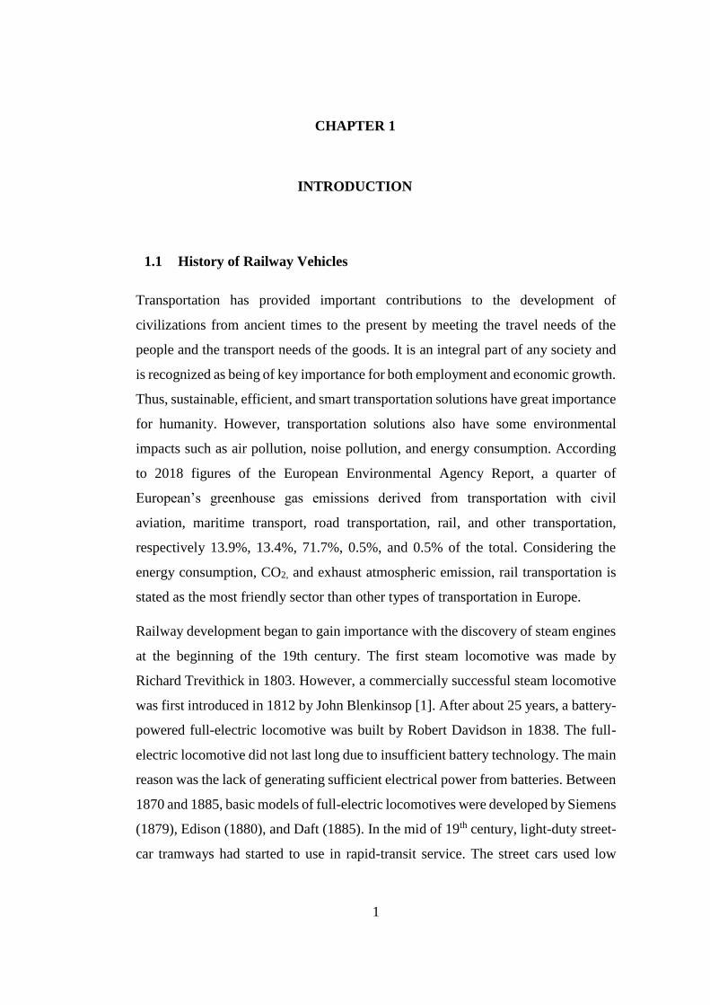
1.1 History of Railway Vehicles

Transportation has provided important contributions to the development of

civilizations from ancient times to the present by meeting the travel needs of the

people and the transport needs of the goods. It is an integral part of any society and

is recognized as being of key importance for both employment and economic growth.

Thus, sustainable, efficient, and smart transportation solutions have great importance

for humanity. However, transportation solutions also have some environmental

impacts such as air pollution, noise pollution, and energy consumption. According

to 2018 figures of the European Environmental Agency Report, a quarter of

European’s greenhouse gas emissions derived from transportation with civil

aviation, maritime transport, road transportation, rail, and other transportation,

respectively 13.9%, 13.4%, 71.7%, 0.5%, and 0.5% of the total. Considering the

energy consumption, CO2, and exhaust atmospheric emission, rail transportation is

stated as the most friendly sector than other types of transportation in Europe.

Railway development began to gain importance with the discovery of steam engines

at the beginning of the 19th century. The first steam locomotive was made by

Richard Trevithick in 1803. However, a commercially successful steam locomotive

was first introduced in 1812 by John Blenkinsop [1]. After about 25 years, a battery-

powered full-electric locomotive was built by Robert Davidson in 1838. The full-

electric locomotive did not last long due to insufficient battery technology. The main

reason was the lack of generating sufficient electrical power from batteries. Between

1870 and 1885, basic models of full-electric locomotives were developed by Siemens

(1879), Edison (1880), and Daft (1885). In the mid of 19th century, light-duty street-

car tramways had started to use in rapid-transit service. The street cars used low

2

voltage DC (LVDC) systems that were supplied by batteries located on the tramways

or supplying DC current from a station through overhead wire or a ground-level rail.

The LVDC electric traction systems of tramway vehicles had a great influence on

the use of electric traction systems on heavy-duty railway vehicles in the following

years. The LVDC electric traction spread to displace steam traction. After a while,

diesel-electric locomotives were introduced as soon as the diesel engine was

presented by Rudolf Diesel [2].

In the last 50 years, there has been a rapid acceleration in railway traction drive

system development in parallel with innovations in the power electronics and

microprocessor fields. Solid-state rectifiers had begun to be used in locomotives

between 1970 and 1973. After that, the tendency to use solid-state products in motor

control systems had increased, and the use of thyristors in DC traction motor control

began in the 1980s. The better tractive effort, better wheel-slip control, higher

efficiency, and weight reduction had been achieved with the use of thyristors. In

addition to this, a prototype of a diesel-electric locomotive that used AC traction

motors was presented in 1971 [2]. Manufacturing of AC traction motors is easier,

and AC traction motors require less maintenance during their operating life. They

also give a higher power to weight ratio and power to volume ratio than the same

power level DC traction motors [3]. Insulated gate bipolar transistors (IGBT)

technology was developed in the 1980s. However, it became commercially

widespread after the 1990s. By using IGBT technology, power quality, power to

weight ratio, and power to volume ratio of traction systems were further increased.

As a result of these developments, old technology traction systems have been

replaced by modern and new technology electric traction systems. The main

advantages of modern electric traction systems are higher energy efficiency, higher

reliability, less noise, lower maintenance, lower operating cost, pollution-free

operation, higher power to weight ratio, and higher power to volume ratio than old

equivalent traction systems. Less weight and volume also provide more free space

for passengers. Thus, the need for innovative and efficient modern traction systems

will increase day by day.

3

The improvement of overall energy efficiency and reliability needs are two of the

most important factors that triggered the development of new semiconductor

technologies. Nowadays, gallium nitride (GaN) and silicon carbide (SiC) based wide

band-gap semiconductor technologies have begun to gain importance in low and

medium power applications [4]–[8]. Higher blocking voltage, higher operating

temperature, and higher switching speed features make SiC-based power MOSFETs

attractive for low and medium power applications by decreasing the volume and

weight of converters and increasing conversion efficiency. In addition to this, wide-

bandgap power products offer a chance to use simpler modulation techniques and

control algorithms. Because of these superior advantages, railway traction-drive

manufacturers such as Mitsubishi, Toshiba, and Hitachi, have a strong tendency to

use SiC semiconductors.

1.1.1 Types of Railway Traction Systems

So far, four main types of traction systems have been built up. These are respectively

steam-powered, electric-powered, diesel-powered, and hybrid traction systems.

Among them, the steam-powered traction systems firstly appeared. These traction

systems were working by burning combustible materials such as coal, wood, and oil.

Those systems had a big disadvantage in terms of air pollution comparing the other

traction systems. From the early 1900s, steam-powered traction systems were

gradually superseded by electric and diesel-powered traction systems. Although full

electric-powered traction systems had been built up earlier and have more

advantages than diesel-powered traction systems, they have been widespread after

diesel-powered traction systems because of the lack of electrification infrastructures.

Typical diesel-powered traction systems are, namely, diesel-mechanical, diesel-

electric, diesel-hydraulic, diesel-steam, and diesel-pneumatic. Diesel-powered

traction systems have many advantages over steam-powered ones, such as easy

start/stop, safely operable by one person, dirt free, low maintenance requirements,

elimination of dependency on an electrification system, and very less capital

investment needs and operational costs. Besides this, compared to electric-powered

4

traction systems, diesel-powered traction systems also have a bad environmental

impact on air pollution, are less powerful and less efficient, creating more audible

noise. Full electric-powered traction systems could only be widespread after the

1970s [9].

The main objectives of technological improvements in railway traction systems are

to increase energy efficiency and reliability and to offer solutions to reduce

environmental damage. In parallel with the development of modern traction

converters, since the 2000s, supercapacitor energy storage systems (ESS) have been

used in railway applications to reduce the energy consumption of the railway

vehicles, to regulate the catenary voltage, and to provide temporarily catenary-free

operation [10], [11]. These systems can be installed on-board or as stationary at

power substations [12]–[15]. The use of energy storage equipment in electric-

powered traction systems is growing up due to the great advantage of decreasing

waste of energy. With the developments of rechargeable energy storage equipment

such as high voltage lithium batteries, supercapacitors, and lithium-ion capacitors,

energy storage systems have been used on power stations, metro, and tram vehicles.

In addition, hybrid diesel-electric powered traction systems equipped with energy

storage systems are becoming widespread on shunting locomotives and diesel-

electric EMUs.

1.1.2 Types of Railway Electrification Systems

Railway electrification systems provide electrical energy to traction and auxiliary

power supply systems located on the railway vehicles. Therefore, they have a very

important role in making electric traction systems usable. Early electrification

systems provide low voltage 600VDC for tramways and light rail vehicles. These

rail vehicles had primitive traction systems consisted of resistors and contactors to

perform speed and torque control of DC electric motors.

Today, several electrification systems exist in the world for different rail vehicles

and can be classified according to voltage and contact system. The most common

5

voltages are 750 VDC, 1500 VDC, 3000 VDC, 15 kVAC (162/3 Hz), 25 kVAC

(50Hz) respectively [16].

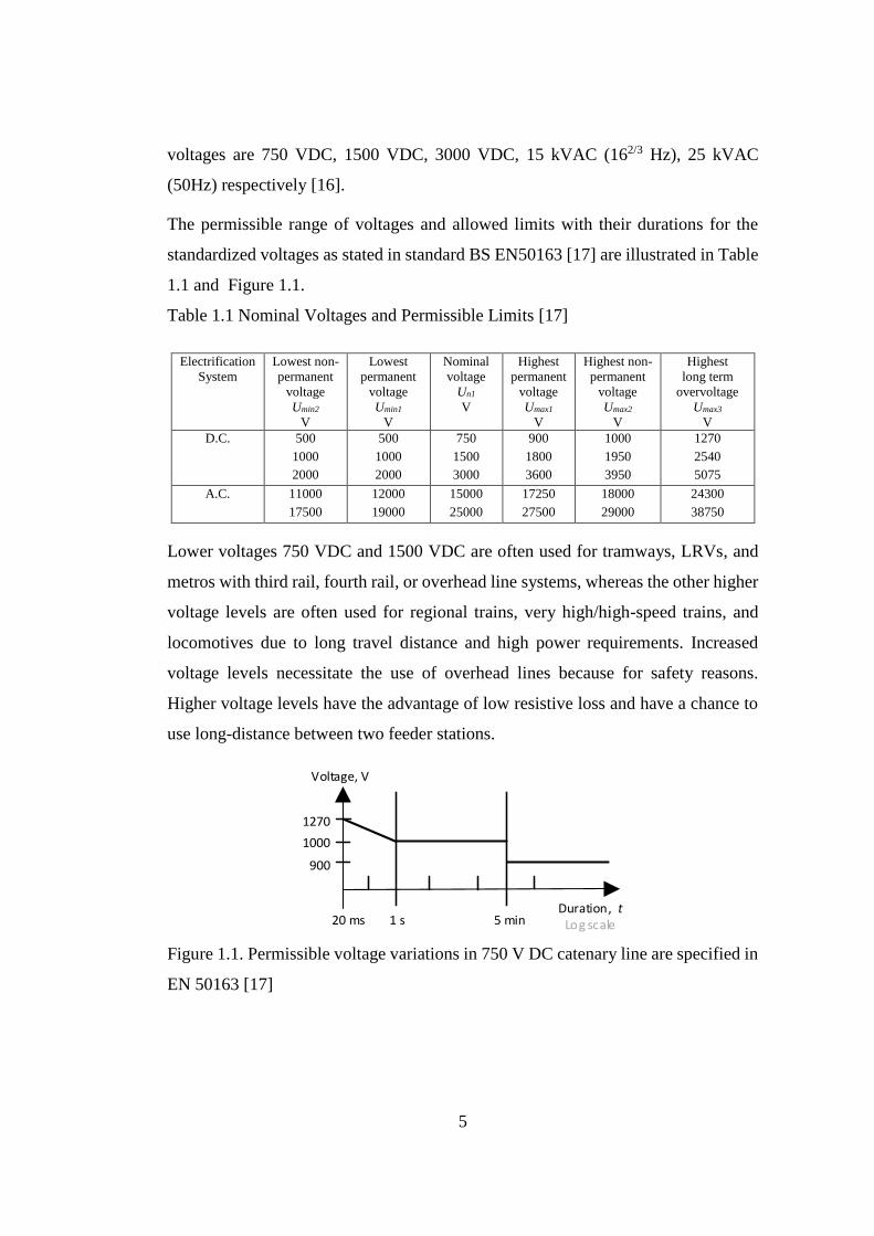
The permissible range of voltages and allowed limits with their durations for the

standardized voltages as stated in standard BS EN50163 [17] are illustrated in Table

1.1 and Figure 1.1.

Table 1.1 Nominal Voltages and Permissible Limits [17]

Electrification

System

Lowest non-

permanent

voltage

Umin2

V

Lowest

permanent

voltage

Umin1

V

Nominal

voltage

Un1

V

Highest

permanent

voltage

Umax1

V

Highest non-

permanent

voltage

Umax2

V

Highest

long term

overvoltage

Umax3

V

D.C. 500

1000

2000

500

1000

2000

750

1500

3000

900

1800

3600

1000

1950

3950

1270

2540

5075

A.C. 11000

17500

12000

19000

15000

25000

17250

27500

18000

29000

24300

38750

Lower voltages 750 VDC and 1500 VDC are often used for tramways, LRVs, and

metros with third rail, fourth rail, or overhead line systems, whereas the other higher

voltage levels are often used for regional trains, very high/high-speed trains, and

locomotives due to long travel distance and high power requirements. Increased

voltage levels necessitate the use of overhead lines because for safety reasons.

Higher voltage levels have the advantage of low resistive loss and have a chance to

use long-distance between two feeder stations.

1270

Duration, t Log scale

Voltage, V

1000

900

20 ms 1 s 5 min

Figure 1.1. Permissible voltage variations in 750 V DC catenary line are specified in

EN 50163 [17]

6

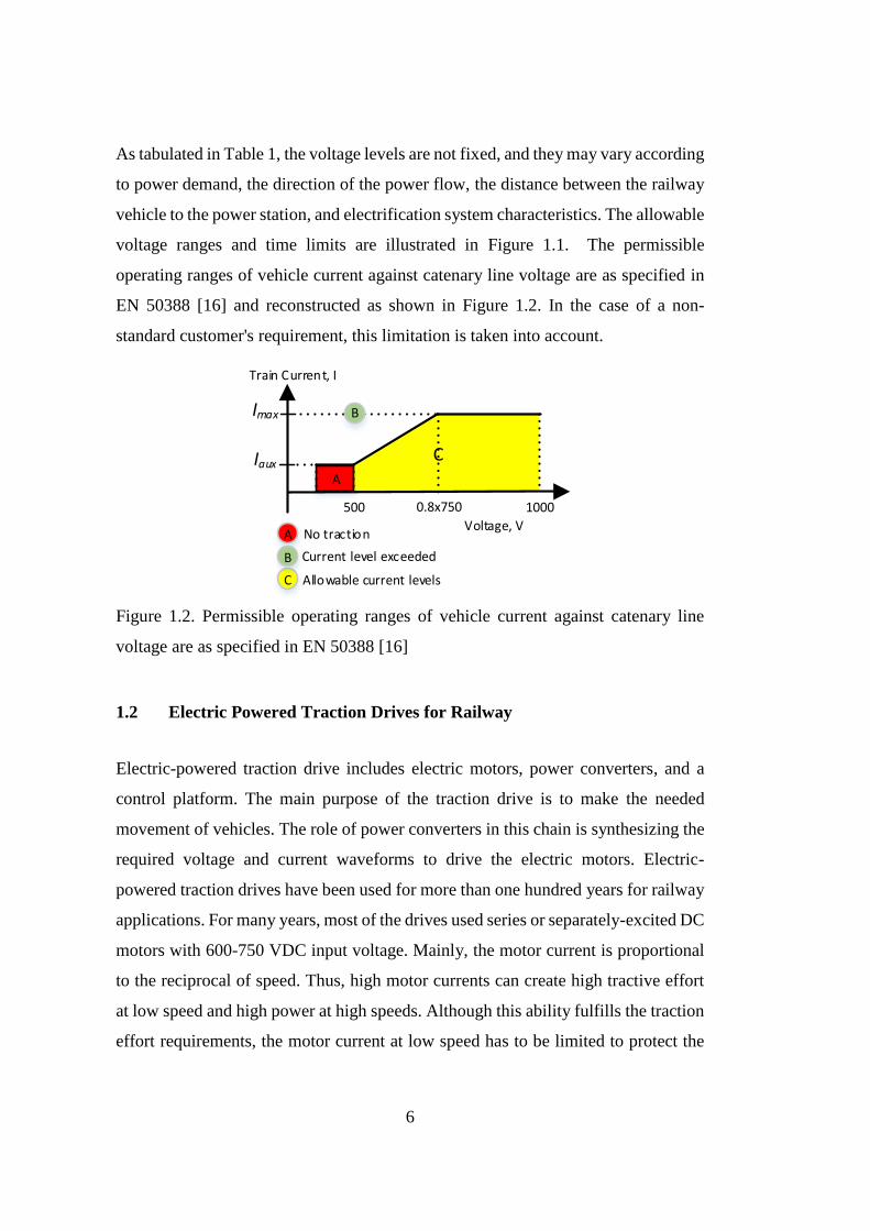
As tabulated in Table 1, the voltage levels are not fixed, and they may vary according

to power demand, the direction of the power flow, the distance between the railway

vehicle to the power station, and electrification system characteristics. The allowable

voltage ranges and time limits are illustrated in Figure 1.1. The permissible

operating ranges of vehicle current against catenary line voltage are as specified in

EN 50388 [16] and reconstructed as shown in Figure 1.2. In the case of a non-

standard customer's requirement, this limitation is taken into account.

Train Current, I

Iaux

10000.8x750500

Imax

A

C

B

No traction

Current level exceeded

Allowable current levels

CA

B

Voltage, V

Figure 1.2. Permissible operating ranges of vehicle current against catenary line

voltage are as specified in EN 50388 [16]

1.2 Electric Powered Traction Drives for Railway

Electric-powered traction drive includes electric motors, power converters, and a

control platform. The main purpose of the traction drive is to make the needed

movement of vehicles. The role of power converters in this chain is synthesizing the

required voltage and current waveforms to drive the electric motors. Electric-

powered traction drives have been used for more than one hundred years for railway

applications. For many years, most of the drives used series or separately-excited DC

motors with 600-750 VDC input voltage. Mainly, the motor current is proportional

to the reciprocal of speed. Thus, high motor currents can create high tractive effort

at low speed and high power at high speeds. Although this ability fulfills the traction

effort requirements, the motor current at low speed has to be limited to protect the

7

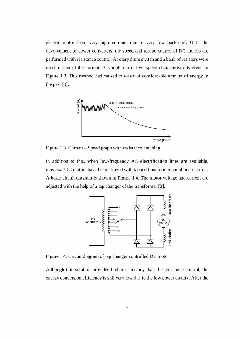
electric motor from very high currents due to very low back-emf. Until the

devolvement of power converters, the speed and torque control of DC motors are

performed with resistance control. A rotary drum switch and a bank of resistors were

used to control the current. A sample current vs. speed characteristic is given in

Figure 1.3. This method had caused to waste of considerable amount of energy in

the past [3].

Cu

rren

t (A

)

Speed (km/h)

Average notching current

Peak notching current

Figure 1.3. Current – Speed graph with resistance notching

In addition to this, when low-frequency AC electrification lines are available,

universal/DC motors have been utilized with tapped transformer and diode rectifier.

A basic circuit diagram is shown in Figure 1.4. The motor voltage and current are

adjusted with the help of a tap changer of the transformer [3].

HV

AC SUPPLY

Sm

oo

thin

g c

ho

ke

Fie

ld w

ind

ing

DC

MOTOR

Figure 1.4. Circuit diagram of tap changer controlled DC motor

Although this solution provides higher efficiency than the resistance control, the

energy conversion efficiency is still very low due to the low power quality. After the

8

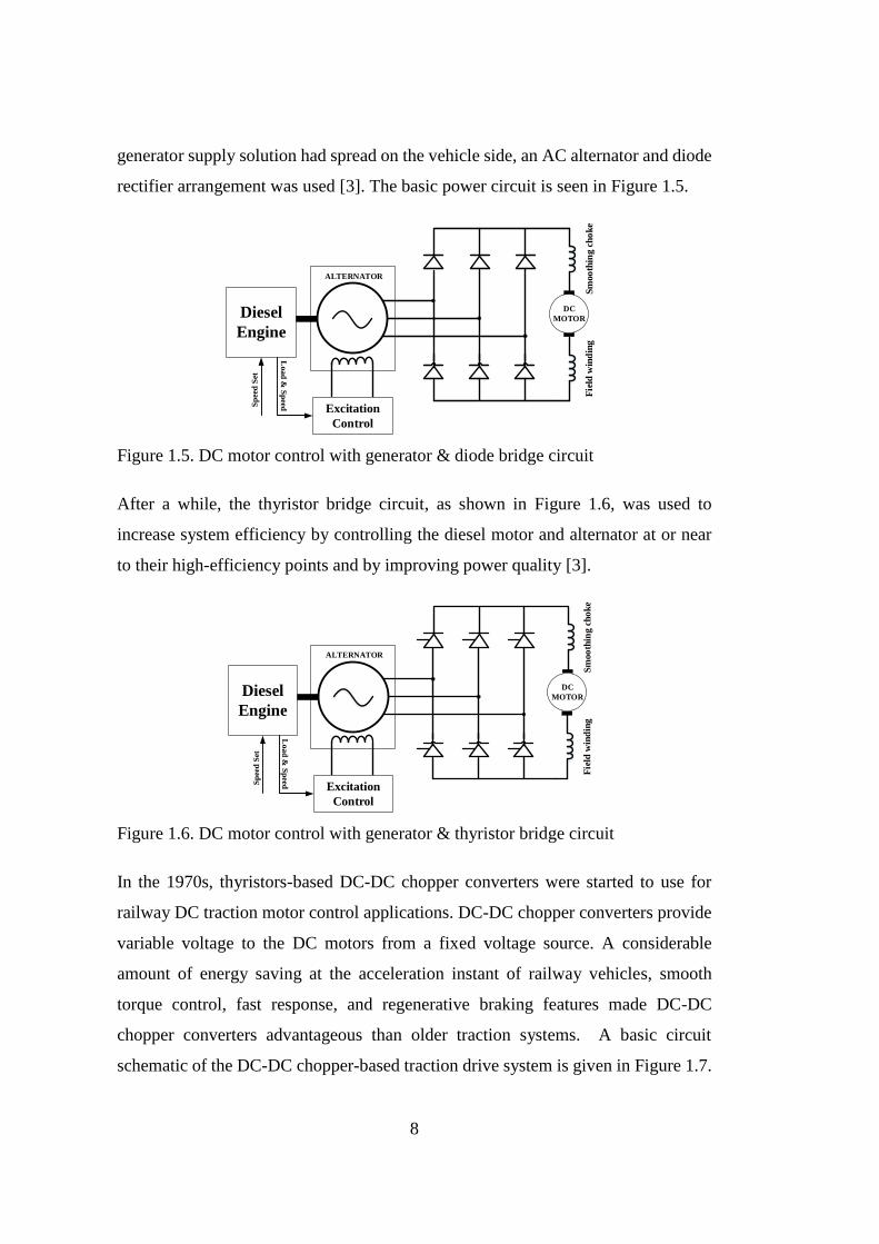
generator supply solution had spread on the vehicle side, an AC alternator and diode

rectifier arrangement was used [3]. The basic power circuit is seen in Figure 1.5.

Sm

oo

thin

g c

ho

ke

Fie

ld w

ind

ing

DC

MOTORDiesel

Engine

Excitation

Control

ALTERNATOR

Load

& S

peedS

pee

d S

et

Figure 1.5. DC motor control with generator & diode bridge circuit

After a while, the thyristor bridge circuit, as shown in Figure 1.6, was used to

increase system efficiency by controlling the diesel motor and alternator at or near

to their high-efficiency points and by improving power quality [3]. S

moo

thin

g c

ho

ke

Fie

ld w

ind

ing

DC

MOTORDiesel

Engine

Excitation

Control

ALTERNATOR

Lo

ad

& S

peedS

pee

d S

et

Figure 1.6. DC motor control with generator & thyristor bridge circuit

In the 1970s, thyristors-based DC-DC chopper converters were started to use for

railway DC traction motor control applications. DC-DC chopper converters provide

variable voltage to the DC motors from a fixed voltage source. A considerable

amount of energy saving at the acceleration instant of railway vehicles, smooth

torque control, fast response, and regenerative braking features made DC-DC

chopper converters advantageous than older traction systems. A basic circuit

schematic of the DC-DC chopper-based traction drive system is given in Figure 1.7.

9

The main thyristor is T1. T2 and T3 are used as auxiliary circuits to divert the current

from T1 to L2 with the help of a resonant circuit in order to switch off T1 [18].

L1

L2

T2

T1

T3

FWD

C

Sm

ooth

ing

Ch

oke

Fie

ld

Win

din

g

DC

MOTOR

CF

LF

Catenary Wire

Wheel

Figure 1.7. DC motor control with thyristor-based DC-DC chopper circuit [18]

Besides this, AC traction motors and gate turn-off (GTO) thyristor-based power

converters were started to use in traction applications at the end of the 1970s with

the developments in semiconductor and microprocessor technology. Since then, the

usage of AC traction motors has spread quickly in railway applications. Figure 1.8

shows the schematic diagram of the inverter circuit [19].

CF

LF

Catenary Wire

Wheel

IM

Figure 1.8. GTO thyristor-based three-phase traction inverter [19]

These developments had made AC traction motors and GTO thyristor-based power

converters more attractive in the past. These traction systems are also called AC

10

traction drives. The advantages of AC traction drives can be expressed as follows by

comparing them with DC traction drives:

- Higher power to volume and power to weight ratio,

- Higher efficiency,

- Low maintenance requirements,

- Higher terminal voltage and shaft speeds due to brushless design,

- Higher immunity for environmental factors such as snow, rain, humidity and

etc.

- More robust mechanical structure.

However, GTO thyristor-based power converters have limited switching frequencies

up to 500 Hz and require complex gate driver circuits. As a result of this, they create

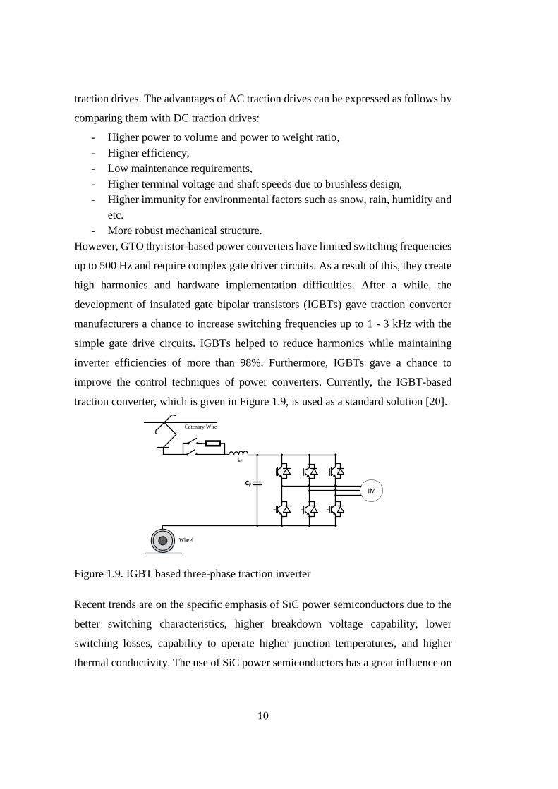
high harmonics and hardware implementation difficulties. After a while, the

development of insulated gate bipolar transistors (IGBTs) gave traction converter

manufacturers a chance to increase switching frequencies up to 1 - 3 kHz with the

simple gate drive circuits. IGBTs helped to reduce harmonics while maintaining

inverter efficiencies of more than 98%. Furthermore, IGBTs gave a chance to

improve the control techniques of power converters. Currently, the IGBT-based

traction converter, which is given in Figure 1.9, is used as a standard solution [20].

CF

LF

Catenary Wire

Wheel

IM

Figure 1.9. IGBT based three-phase traction inverter

Recent trends are on the specific emphasis of SiC power semiconductors due to the

better switching characteristics, higher breakdown voltage capability, lower

switching losses, capability to operate higher junction temperatures, and higher

thermal conductivity. The use of SiC power semiconductors has a great influence on

11

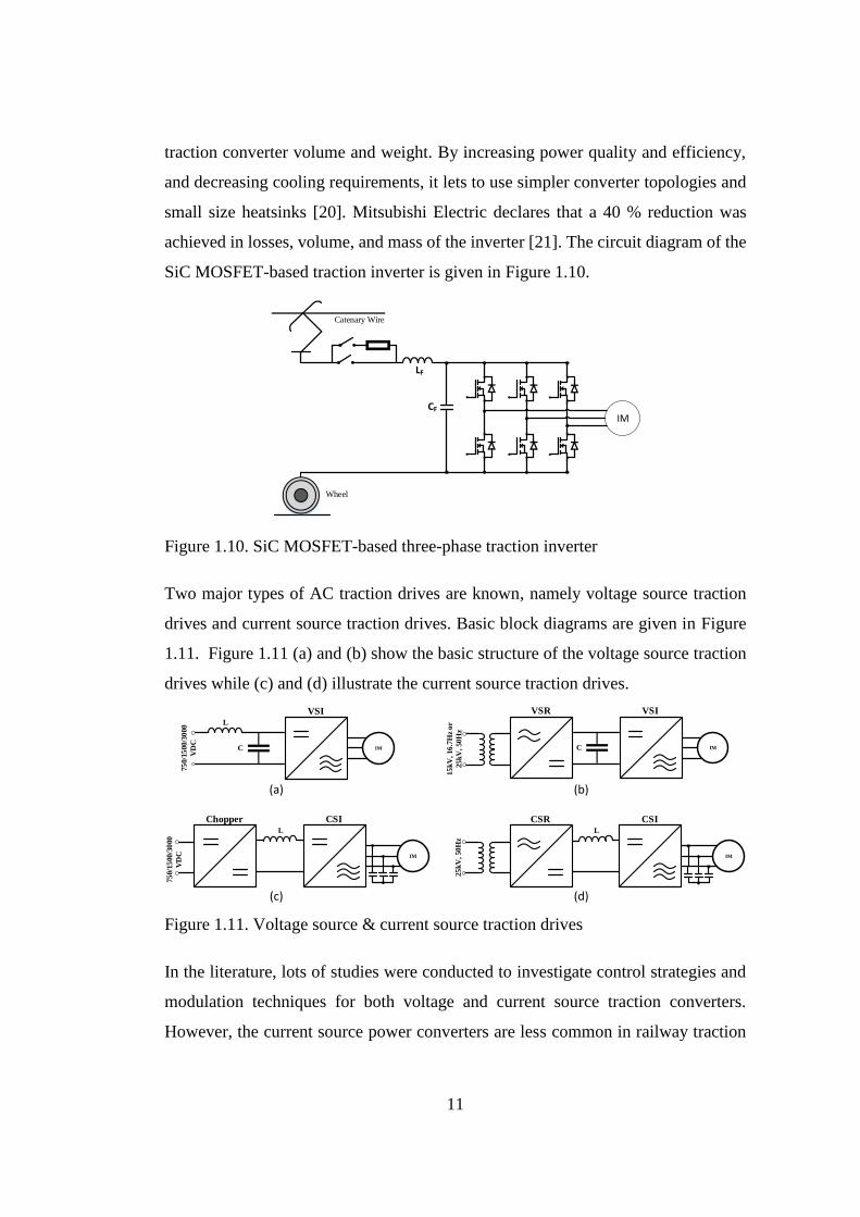
traction converter volume and weight. By increasing power quality and efficiency,

and decreasing cooling requirements, it lets to use simpler converter topologies and

small size heatsinks [20]. Mitsubishi Electric declares that a 40 % reduction was

achieved in losses, volume, and mass of the inverter [21]. The circuit diagram of the

SiC MOSFET-based traction inverter is given in Figure 1.10.

CF

LF

Catenary Wire

Wheel

IM

Figure 1.10. SiC MOSFET-based three-phase traction inverter

Two major types of AC traction drives are known, namely voltage source traction

drives and current source traction drives. Basic block diagrams are given in Figure

1.11. Figure 1.11 (a) and (b) show the basic structure of the voltage source traction

drives while (c) and (d) illustrate the current source traction drives.

VSIL

C

75

0/1

500/3

000

VD

C

IM

L

CSI

IM

Chopper

75

0/1

500/3

000

VD

C

L

CSI

IM

CSR

25

kV

, 50

Hz

VSI

C IM

VSR

15

kV

, 16

.7H

z o

r

25

kV

, 50

Hz

(a) (b)

(c) (d)

Figure 1.11. Voltage source & current source traction drives

In the literature, lots of studies were conducted to investigate control strategies and

modulation techniques for both voltage and current source traction converters.

However, the current source power converters are less common in railway traction

12

applications [22], [23]. For these applications, voltage source power converters are

preferred due to the following superior features [24]:

- Ease of control,

- Low cost,

- Excellent dynamic performance,

- Small size,

- Lower total losses due to the lack of bulky inductive components.

In addition to this, AC traction drives are classified in the literature according to the

voltage levels of converters, namely two-level and multilevel converters.

Classification of different types of traction converter topologies is illustrated in

Figure 1.12.

Traction Converte rs

Voltage SourceCurrent Source

Multilevel Converters Two-level Converters

NPC/A-NPC T-type Flying Capacitor Cascaded H-Bridge

Figure 1.12. Traction converter topologies [24]

From the past, multilevel converters have been commonly used for medium voltage

and medium power drive applications due to the lack of sufficient blocking voltages

of semiconductors. In 1981s, a three-level neutral point clamped converter was

introduced from A. Nabae, I. Takahashi, and H, Akagi. Years later, the multilevel

converter technology, which is composed of several full-bridge converters connected

serially, was presented. These converters, which appeared in 2002, are called

modular multilevel converters [25]–[28]. Flying capacitor multilevel converter was

also developed in the same years.

13

Multilevel converters gave a chance to use series-connected semiconductors with

lower blocking voltages. Because of the applied lower voltage steps, the output

voltage waveform quality is increased, and stresses on electric motor and traction

transformers are decreased by a certain amount. However, on the other hand, the

number of semiconductors, converter complexity, and isolated gate driver need is

increased. Due to the increased number of components, the reliability of the

converter decreases.

The frequently used multilevel traction converter topologies are described in the next

section. With the increased blocking voltages of semiconductors, the world’s leading

traction drive designer companies have switched to two-level voltage source

converter solutions. Multilevel traction converters are preferred in applications with

a power level of 1.5 MVA / 2000 V and above or in applications requiring high

current control bandwidth. Todays, the classical two-level voltage source AC

traction drives are commonly used in railway traction drive applications [24].

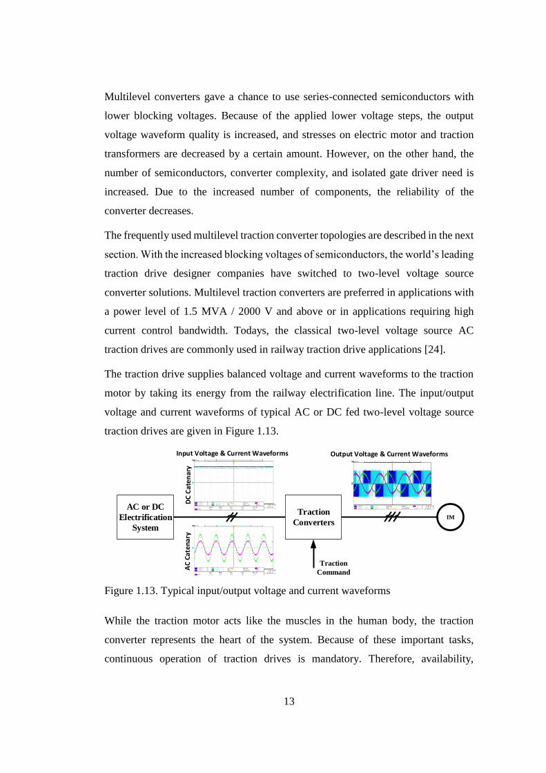
The traction drive supplies balanced voltage and current waveforms to the traction

motor by taking its energy from the railway electrification line. The input/output

voltage and current waveforms of typical AC or DC fed two-level voltage source

traction drives are given in Figure 1.13.

Input Voltage & Current Waveforms

AC

Ca

ten

ary

DC

Ca

ten

ary

Output Voltage & Current Waveforms

Traction

Command

AC or DC

Electrification

System

IMTraction

Converters

Figure 1.13. Typical input/output voltage and current waveforms

While the traction motor acts like the muscles in the human body, the traction

converter represents the heart of the system. Because of these important tasks,

continuous operation of traction drives is mandatory. Therefore, availability,

14

reliability, performance, and lifetime constitute important criteria for traction drive

chain equipment.

1.3 Today’s Power Converters for Railway Traction Drive

Demands for low volume, light weight, high reliability, high power, low cost, and

high efficiency in railway traction are continuously increasing [29]–[31]. Due to

these demands, the developments of semiconductor technologies and power

converter topologies in the field of power electronics have been triggered. This

section shows an overview of recently used power converter topologies for railway

traction.

In order to decrease cost and complexity and increase reliability, the traction

converter manufacturers primarily offer solutions by using simple power converter

topologies together with mature and cheap semiconductor technologies. This

approach provides to takes advantage of the simplest two-level converter topologies

and their simple control methods. Simple hardware structures and control

architecture of two-level converter topologies provide a chance for easy

implementation. In addition to this, fewer component counts help to increase

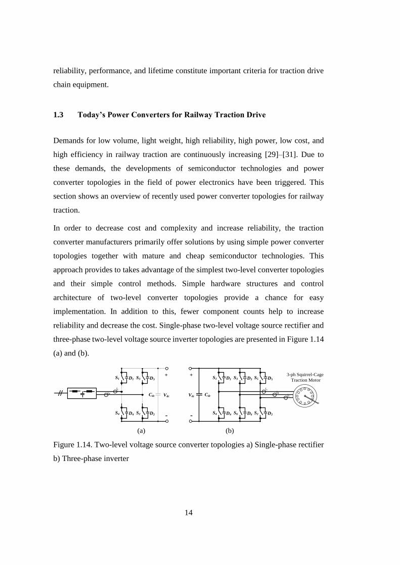
reliability and decrease the cost. Single-phase two-level voltage source rectifier and

three-phase two-level voltage source inverter topologies are presented in Figure 1.14

(a) and (b).

iL

+

-

S1

Cdc

D1

Vdc

S3 D3

S4 D4 S2 D2

iN

iA

+

-

3-ph Squirrel-Cage

Traction MotorS1

Cdc

D1

Vdc

S3 D3 S5 D5

S4 D4 S6 D6 S2 D2

iBiC

(a) (b)

Figure 1.14. Two-level voltage source converter topologies a) Single-phase rectifier

b) Three-phase inverter

15

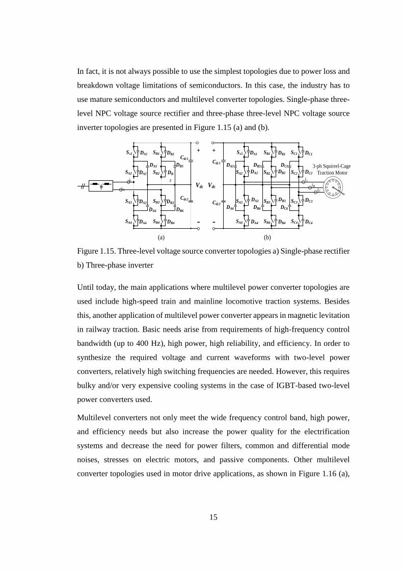
In fact, it is not always possible to use the simplest topologies due to power loss and

breakdown voltage limitations of semiconductors. In this case, the industry has to

use mature semiconductors and multilevel converter topologies. Single-phase three-

level NPC voltage source rectifier and three-phase three-level NPC voltage source

inverter topologies are presented in Figure 1.15 (a) and (b).

iL

+

-

SA2 DA2

Vdc

SB2 DB

2

SA3 DA3 SB3 DB3

iN

SA4 DA4 SB4 DB4

SA1 DA1 SB1 DB1

Cdc2

DA5

DA6

DB5

DB6

Cdc1

3-ph Squirrel-Cage

Traction Motor

+

-

SA2 DA2

Vdc

SB2 DB2

SA3DA3 SB3

DB3

SA4 DA4 SB4 DB4

SA1 DA1 SB1 DB1

Cdc2

Cdc1 DA5

DA6

DB5

DB6

SC2 DC2

SC3DC3

SC4 DC4

SC1 DC1

DC5

DC6

iA

iB

iC

(a) (b)

Figure 1.15. Three-level voltage source converter topologies a) Single-phase rectifier

b) Three-phase inverter

Until today, the main applications where multilevel power converter topologies are

used include high-speed train and mainline locomotive traction systems. Besides

this, another application of multilevel power converter appears in magnetic levitation

in railway traction. Basic needs arise from requirements of high-frequency control

bandwidth (up to 400 Hz), high power, high reliability, and efficiency. In order to

synthesize the required voltage and current waveforms with two-level power

converters, relatively high switching frequencies are needed. However, this requires

bulky and/or very expensive cooling systems in the case of IGBT-based two-level

power converters used.

Multilevel converters not only meet the wide frequency control band, high power,

and efficiency needs but also increase the power quality for the electrification

systems and decrease the need for power filters, common and differential mode

noises, stresses on electric motors, and passive components. Other multilevel

converter topologies used in motor drive applications, as shown in Figure 1.16 (a),

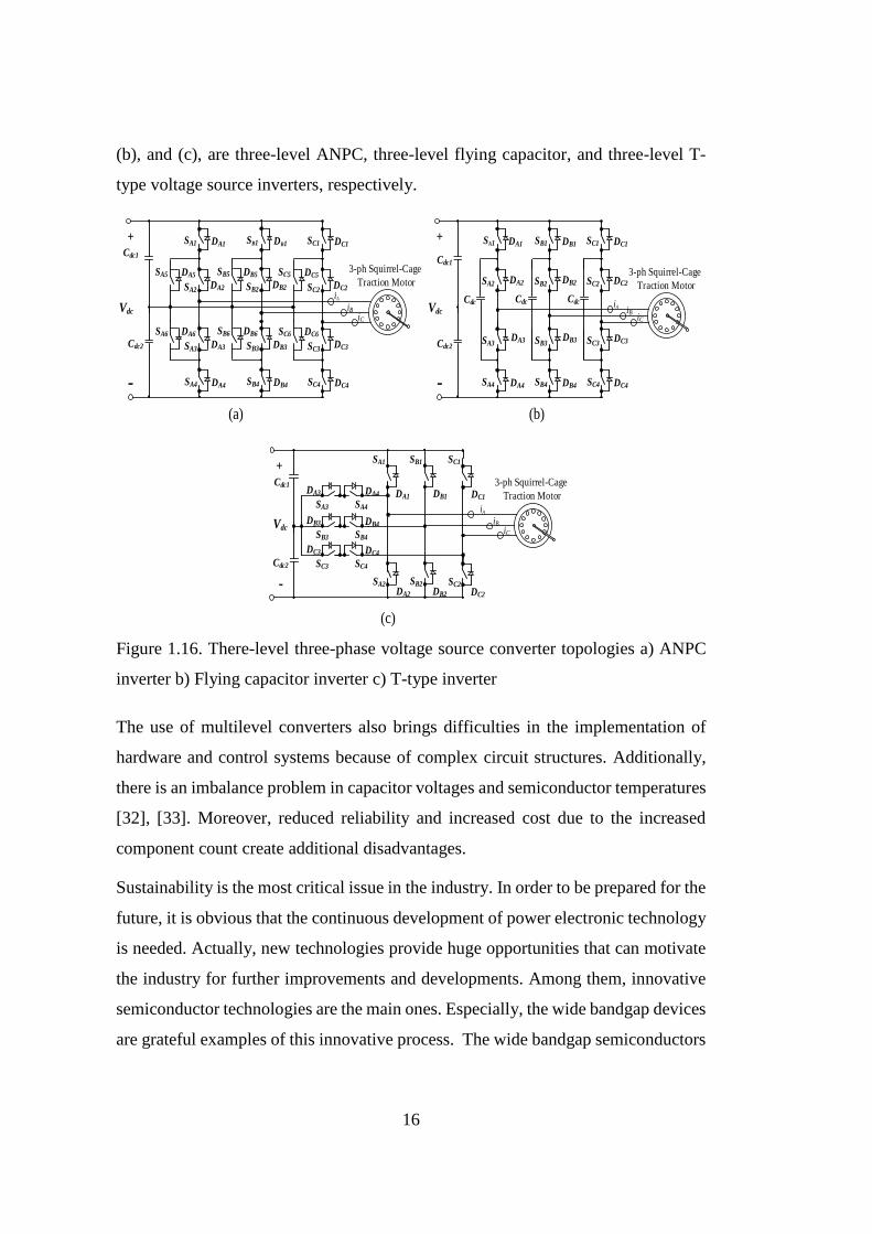
16

(b), and (c), are three-level ANPC, three-level flying capacitor, and three-level T-

type voltage source inverters, respectively.

Cdc1

SA2DA2

iA CdcCdc Cdc

3-ph Squirrel-Cage

Traction Motor

+

-

SA2 DA2

Vdc

SB2 DB2

SA3DA3 SB3

DB3

SA4 DA4 SB4 DB4

SA1 DA1 SB1 DB1

Cdc2

Cdc1

SC2 DC2

SC3DC3

SC4 DC4

SC1 DC1

iA iBiC

3-ph Squirrel-Cage

Traction Motor

+

-

Vdc

Cdc2

Cdc1

DC2SC2

SC3DC3

SC4 DC4

SC1 DC1

iB

iC

SC5 DC5

SC6 DC6

DB2SB2

SB3 DB3

SB4 DB4

SB1 DB1

SB5 DB5

SB6 DB6

DA2SA2

SA3 DA3

SA4 DA4

SA1 DA1

SA5 DA5

SA6 DA6

(a) (b)

iA

3-ph Squirrel-Cage

Traction Motor

+

-

Vdc

Cdc2

DC1

SC1

SC2

DC2

iB

iC

DB1

SB1

SB2

DB2

DA1

SA1

(c)

SA3

DA3

SA4

DA4

SB3

DB3

SB4

DB4

SC3

DC3

SC4

DC4

Figure 1.16. There-level three-phase voltage source converter topologies a) ANPC

inverter b) Flying capacitor inverter c) T-type inverter

The use of multilevel converters also brings difficulties in the implementation of

hardware and control systems because of complex circuit structures. Additionally,

there is an imbalance problem in capacitor voltages and semiconductor temperatures

[32], [33]. Moreover, reduced reliability and increased cost due to the increased

component count create additional disadvantages.

Sustainability is the most critical issue in the industry. In order to be prepared for the

future, it is obvious that the continuous development of power electronic technology

is needed. Actually, new technologies provide huge opportunities that can motivate

the industry for further improvements and developments. Among them, innovative

semiconductor technologies are the main ones. Especially, the wide bandgap devices

are grateful examples of this innovative process. The wide bandgap semiconductors

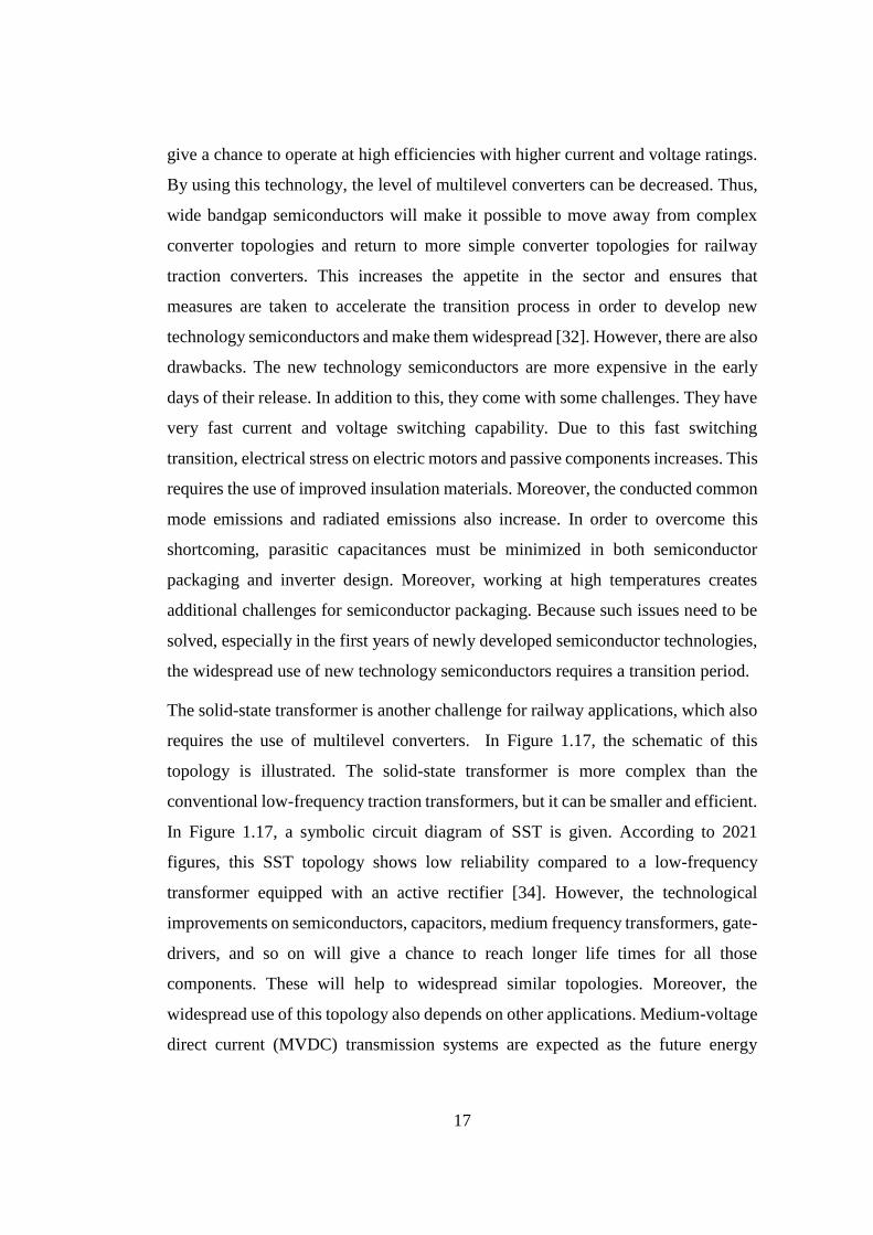
17

give a chance to operate at high efficiencies with higher current and voltage ratings.

By using this technology, the level of multilevel converters can be decreased. Thus,

wide bandgap semiconductors will make it possible to move away from complex

converter topologies and return to more simple converter topologies for railway

traction converters. This increases the appetite in the sector and ensures that

measures are taken to accelerate the transition process in order to develop new

technology semiconductors and make them widespread [32]. However, there are also

drawbacks. The new technology semiconductors are more expensive in the early

days of their release. In addition to this, they come with some challenges. They have

very fast current and voltage switching capability. Due to this fast switching

transition, electrical stress on electric motors and passive components increases. This

requires the use of improved insulation materials. Moreover, the conducted common

mode emissions and radiated emissions also increase. In order to overcome this

shortcoming, parasitic capacitances must be minimized in both semiconductor

packaging and inverter design. Moreover, working at high temperatures creates

additional challenges for semiconductor packaging. Because such issues need to be

solved, especially in the first years of newly developed semiconductor technologies,

the widespread use of new technology semiconductors requires a transition period.

The solid-state transformer is another challenge for railway applications, which also

requires the use of multilevel converters. In Figure 1.17, the schematic of this

topology is illustrated. The solid-state transformer is more complex than the

conventional low-frequency traction transformers, but it can be smaller and efficient.

In Figure 1.17, a symbolic circuit diagram of SST is given. According to 2021

figures, this SST topology shows low reliability compared to a low-frequency

transformer equipped with an active rectifier [34]. However, the technological

improvements on semiconductors, capacitors, medium frequency transformers, gate-

drivers, and so on will give a chance to reach longer life times for all those

components. These will help to widespread similar topologies. Moreover, the

widespread use of this topology also depends on other applications. Medium-voltage

direct current (MVDC) transmission systems are expected as the future energy

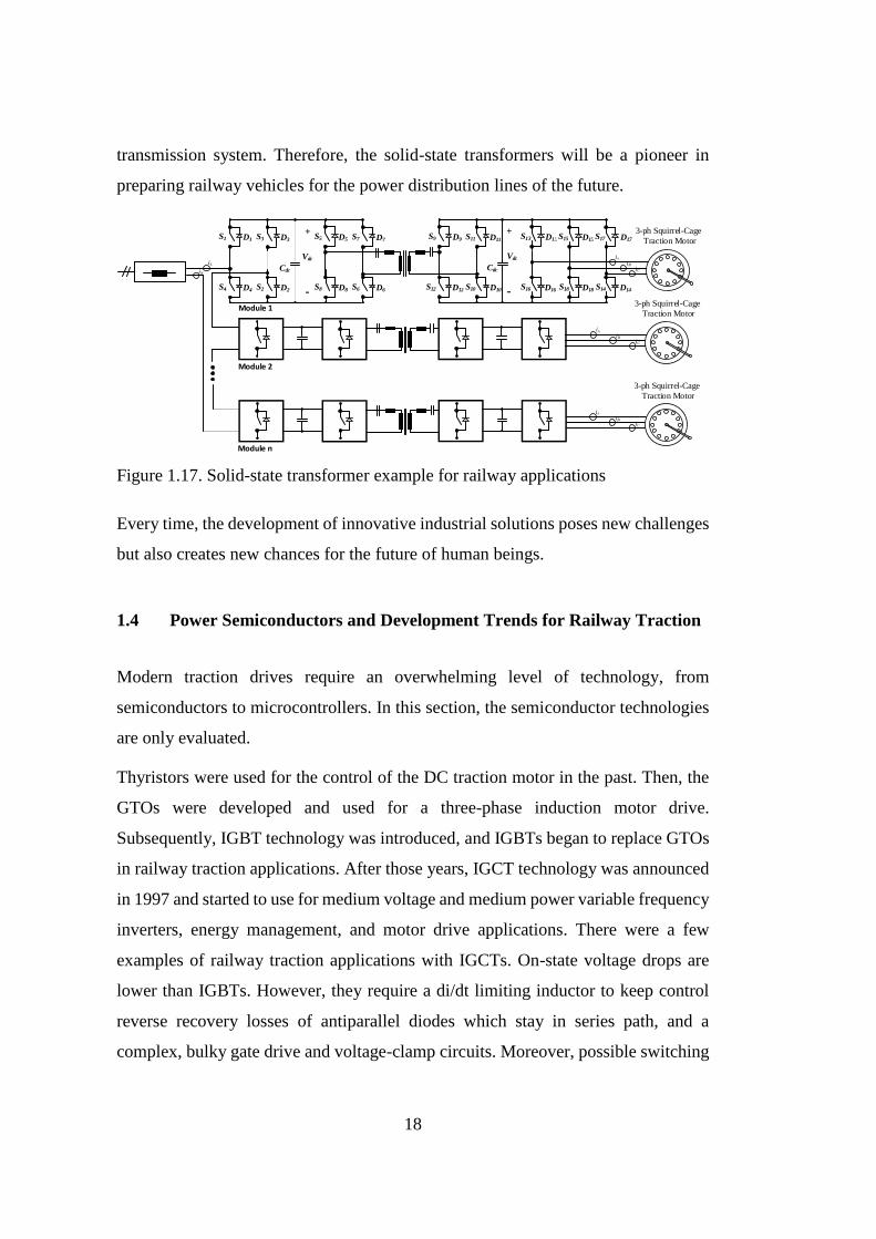
18

transmission system. Therefore, the solid-state transformers will be a pioneer in

preparing railway vehicles for the power distribution lines of the future.

Cdc

iL

-

Vdc

S4 D4 S2 D2

iN

S7 D7

S8 D8 S6 D6

Module 1

Module 2

Module n

S3 D3S1 D1

+S5 D5 S11 D11

S12 D12 S10 D10

S9 D9

Cdc

-

Vdc

+

iA

3-ph Squirrel-Cage

Traction MotorS13 D13 S15 D15 S17 D17

S16 D16 S18 D18 S14 D14

iB

iC

iA

3-ph Squirrel-Cage

Traction Motor

iB

iC

iA

3-ph Squirrel-Cage

Traction Motor

iB

iC

Figure 1.17. Solid-state transformer example for railway applications

Every time, the development of innovative industrial solutions poses new challenges

but also creates new chances for the future of human beings.

1.4 Power Semiconductors and Development Trends for Railway Traction

Modern traction drives require an overwhelming level of technology, from

semiconductors to microcontrollers. In this section, the semiconductor technologies

are only evaluated.

Thyristors were used for the control of the DC traction motor in the past. Then, the

GTOs were developed and used for a three-phase induction motor drive.

Subsequently, IGBT technology was introduced, and IGBTs began to replace GTOs

in railway traction applications. After those years, IGCT technology was announced

in 1997 and started to use for medium voltage and medium power variable frequency

inverters, energy management, and motor drive applications. There were a few

examples of railway traction applications with IGCTs. On-state voltage drops are

lower than IGBTs. However, they require a di/dt limiting inductor to keep control

reverse recovery losses of antiparallel diodes which stay in series path, and a

complex, bulky gate drive and voltage-clamp circuits. Moreover, possible switching

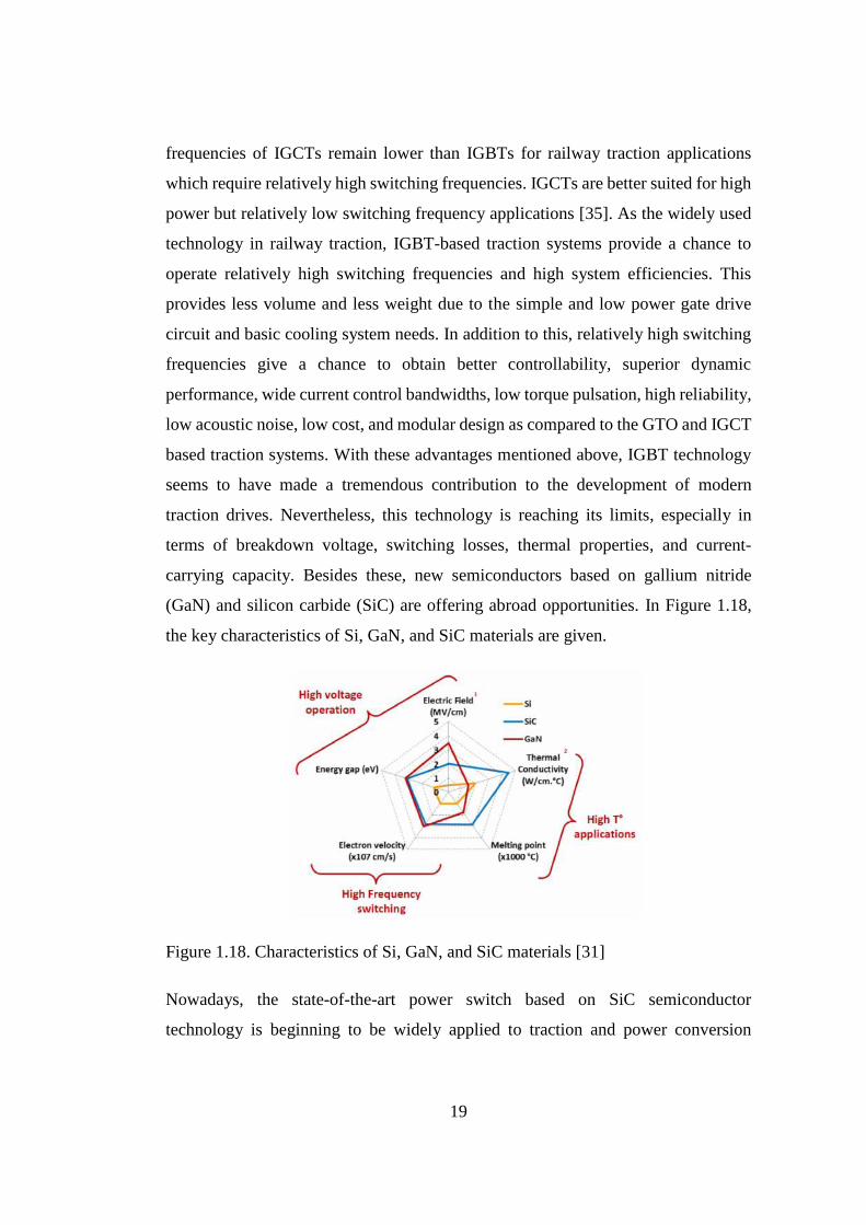
19

frequencies of IGCTs remain lower than IGBTs for railway traction applications

which require relatively high switching frequencies. IGCTs are better suited for high

power but relatively low switching frequency applications [35]. As the widely used

technology in railway traction, IGBT-based traction systems provide a chance to

operate relatively high switching frequencies and high system efficiencies. This

provides less volume and less weight due to the simple and low power gate drive

circuit and basic cooling system needs. In addition to this, relatively high switching

frequencies give a chance to obtain better controllability, superior dynamic

performance, wide current control bandwidths, low torque pulsation, high reliability,

low acoustic noise, low cost, and modular design as compared to the GTO and IGCT

based traction systems. With these advantages mentioned above, IGBT technology

seems to have made a tremendous contribution to the development of modern

traction drives. Nevertheless, this technology is reaching its limits, especially in

terms of breakdown voltage, switching losses, thermal properties, and current-

carrying capacity. Besides these, new semiconductors based on gallium nitride

(GaN) and silicon carbide (SiC) are offering abroad opportunities. In Figure 1.18,

the key characteristics of Si, GaN, and SiC materials are given.

Figure 1.18. Characteristics of Si, GaN, and SiC materials [31]

Nowadays, the state-of-the-art power switch based on SiC semiconductor

technology is beginning to be widely applied to traction and power conversion

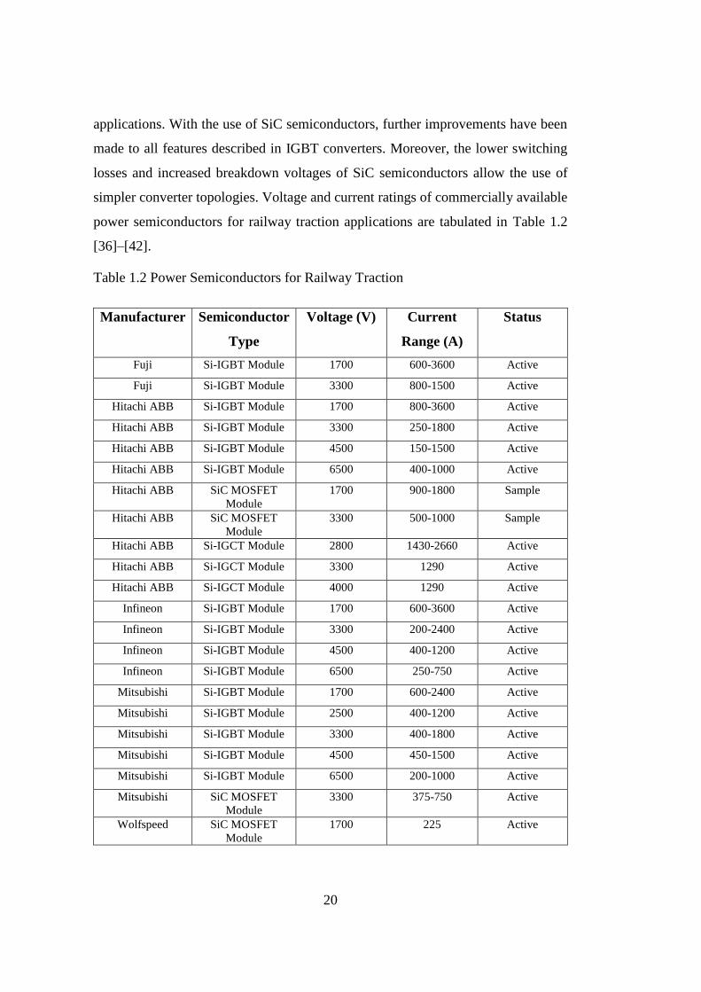
20

applications. With the use of SiC semiconductors, further improvements have been

made to all features described in IGBT converters. Moreover, the lower switching

losses and increased breakdown voltages of SiC semiconductors allow the use of

simpler converter topologies. Voltage and current ratings of commercially available

power semiconductors for railway traction applications are tabulated in Table 1.2

[36]–[42].

Table 1.2 Power Semiconductors for Railway Traction

Manufacturer Semiconductor

Type

Voltage (V) Current

Range (A)

Status

Fuji Si-IGBT Module 1700 600-3600 Active

Fuji Si-IGBT Module 3300 800-1500 Active

Hitachi ABB Si-IGBT Module 1700 800-3600 Active




Hitachi ABB SiC MOSFET

Module

1700 900-1800 Sample

Hitachi ABB SiC MOSFET

Module

3300 500-1000 Sample

Hitachi ABB Si-IGCT Module 2800 1430-2660 Active

Hitachi ABB Si-IGCT Module 3300 1290 Active

Hitachi ABB Si-IGCT Module 4000 1290 Active

Infineon Si-IGBT Module 1700 600-3600 Active




Mitsubishi Si-IGBT Module 1700 600-2400 Active





Mitsubishi SiC MOSFET

Module

3300 375-750 Active

Wolfspeed SiC MOSFET

Module

1700 225 Active

21

In Table 1.3, these switches are qualitatively compared according to their native

characteristics [43]–[49].

Table 1.3 Semiconductor Comparison

Si-IGBT Module Si-IGCT

SiC MOSFET Module

Impact

Snubber need No Yes Yes Power density

On-state voltage Moderate Low Low Power density

Current density Moderate High High Power density

Gate driver difficulty Low Moderate Low Power density

Switching frequency <3kHz <1kHz <20kHz Power density

Failure mode Open Short Open Reliability

Short-circuit current Gate driver

limited Snubber limited

Gate driver limited Reliability

Series connection Easier Moderate Easier Reliability

Parallel connection Moderate Difficult Easier Reliability

Thermal cycling capacity Moderate High High Reliability

The switching frequencies could not be increased due to the high switching losses of

previously existing power semiconductors and switching frequencies that remain

significantly lower than today's state-of-the-art semiconductors. This results in low

power quality (i.e., high amount of harmonics), poor system efficiency, torque

pulsation, narrow current control bandwidths, and slow response.

High switching frequencies can be considered more suitable for traction applications

requiring relatively wide current (i.e., torque) control bandwidth and high power

quality (e.g., low-frequency harmonics are significantly reduced). Wide control

bandwidth helps to increase system stability. In addition to this, lower motor current

harmonics lead to increase system efficiencies. With the improvements of

semiconductors and microprocessors, intelligent modulation methods, voltage, and

current control algorithms have been developed. In the future, higher control

22

bandwidths that can be achieved with innovative control algorithms and

semiconductor technology will also help traction motors to operate at very high

speeds. This may help to reduce traction motor volume and weights. With the

continuously increasing switching frequency capability of the power

semiconductors, the power electronic converters will provide more benefits at the

system levels.

In addition, short circuit protection, overload, thermal cycling, and power cycling

capabilities, easy series and parallel operation, power density, and safe state of power

semiconductors under fault conditions create other important requirements for

railway traction applications. Parallel to the above features and being commercially

available, IGBTs appear to be widely used in traction applications. However, on the

other hand, when SiC MOSFETs become widespread, it is seen that IGBTs will be

replaced by SiC MOSFETs.

1.5 Problem Statement and Motivation

In the railway industry, operators typically compare several features such as driving

performance, load capacity, passenger comfort, initial and operating cost, reliability,

availability, and maintainability. All operators know the importance of energy

consumption to decrease operating cost.

A reduction in energy consumption should be achieved without resulting in setbacks

with respect to the features such as driving performance, load capacity, comfort,

operating cost, reliability, availability, and maintainability. Up to now, many

electric-powered railway traction systems have been built around the world. As of

today, most of the electric-powered traction systems widely use silicon-based

insulated-gate bipolar transistors (IGBT). In medium power drives, like electric-

powered traction systems, the switching frequency of IGBTs is limited to between

500-3000 Hz due to the considerable amount of switching losses. This restriction

creates many problems. Low-order harmonics may appear due to low switching

frequencies. This situation decreases power quality and overall energy conversion

23

efficiency and creates torque ripple at integer multiples of the fundamental

frequency. In order to eliminate this low order harmonics, special pulse width

modulation techniques such as Selective Harmonic Elimination (SHE), Selective

Harmonic Mitigation (SHM), Optimum Pulse Width Modulation (OPWM), and etc.

have to be used. However, this necessity makes the control algorithms and

modulation techniques complex. In addition, the elimination of low order harmonics

may still not be possible due to the limit of effective switching frequency if the

fundamental frequency of the output waveforms is quite high as usual in motor drive

applications. In this case, the pulse number has to be decreased because of the

effective switching frequency reached in such modulation methods. Anymore,

torque ripples and motor losses cannot be reduced. This ends up with a decrease in

overall system efficiency and an increase in operating cost. Moreover, lower

switching frequencies also yield narrow current and torque control bandwidth. This

makes poorer the system stability. All these issues show that resulting in some

setbacks are inevitable with IGBT-based two-level power converters. Such problems

can be solved with IGBT-based multilevel converters, as described in the previous

section. However, this time the complexity of the hardware and control algorithms

increases. In addition, the reliability decreases as the number of components

increases.

Nowadays, SiC semiconductor technology has begun to gain importance in the

application of power electronics. SiC semiconductor-based traction systems provide

promising opportunities for energy saving and better power quality. The SiC-based

power switches give a chance to reduce switching losses and increase operating

temperature. This situation leads to increased efficiency, power to weight, and power

to volume ratio by decreasing cooling system requirements. Besides this, SiC-based

power switches allow operating high switching frequencies at higher voltage and

current levels. This makes it possible to use simpler converter topologies instead of

multilevel topologies, eliminate complex control algorithms and low order

harmonics and increase current control bandwidths. Especially, this new technology

which attracts the attention of the academy and the industry has many issues that

24

need to be researched in terms of application areas such as traction and propulsion

drives, medium voltage industrial drives, medium voltage DC and high voltage DC

energy transmission systems.

1.6 Scope of the Thesis

In this thesis, it is aimed to significantly reduce control system complexity, increase

efficiency and power density by providing high-quality ac currents at higher output

fundamental frequencies. In order to achieve this target, all SiC power MOSFET-

based 500-900 VDC, 165 kVA two-level traction inverter has been developed and

implemented. The capabilities of the developed system have been investigated by

simulations and laboratory test studies. Field-oriented control method and space

vector pulse width modulation technique has been implemented to control traction

motor. The prototype system is composed of a power electronic block, inverter

control unit, voltage and current transducers, LC input filter, cooling system, main

line contactor, soft start contactor, and resistor. The cut-off frequency of the low pass

filter is set below the mains frequency. An air-core line reactor is chosen as the input

filter element in order to prevent magnetic saturation under short-circuit failure

cases. This feature is very important to limit the current in the event of a short-circuit.

New technology semiconductors are used to build the power electronics block in the

simplest form. 10 kHz switching frequency is used to minimize the current

harmonics even at the higher output fundamental frequencies. This study is the first

example of a SiC power MOSFET-based traction drive developed for rail

transportation vehicles in Turkey.

In addition to this, the effects of SiC power semiconductors on the selection of

converter topologies, passive components, cooling systems, motor windings, and

bearings are discussed. Moreover, the impact of SiC-based power converters on the

copper and iron losses in the motor is explored systematically.

In order to validate these effects on motor drive applications, a full-scale physical

simulator for all-SiC traction motor drive was designed and implemented. This test

https://ieeexplore.ieee.org/document/8830470/

https://ieeexplore.ieee.org/document/8830470/

25

setup is equipped with software programs for a catenary model, rail track model, and

vehicle model and permits the performance verification of various control,

modulation, and energy-saving strategies. Finally, laboratory tests are conducted on

this setup.

This research work makes following original contributions to voltage source

inverters in railway applications:

one of the first design and development works of all silicon carbide (SiC)

traction converter for new generation light rail transportation systems,

presentation of qualitative design criteria based on analysis, simulation and

experimental work for SiC power MOSFET based traction converter,

first design and implementation of a full scale physical simulator of an all

SiC traction motor drive for LRTS with on-board super-capacitor energy

storage system,

verification of designed new generation traction converter with full scale

physical simulator.

The outline of the thesis is given below:

In Chapter 2, a description of light rail transportation systems, system architectures,

traction motors, operating principles of two and three-level voltage source traction

inverters, control methods, and modulation techniques are presented.

In Chapter 3, the design methodology of the traction inverter is described. The design

requirements of the prototype system are stated. The selection of the critical

components is explained. Semiconductor power loss calculations are investigated for

two-level and three-level traction inverter topologies with candidate semiconductors.

The overall system efficiencies are investigated. Traction inverter power block

design is illustrated. The motor control algorithm, including active resonant

damping, is presented.

In Chapter 4, the modeling studies of the MOSFET module, traction drive system,

and test setup are presented. Modeling studies of the rail vehicle and track are briefly

26

explained and the method used to derive the system requirements is defined. The

simulation results under steady-state and dynamic regimes are investigated.

In Chapter 5, the design and the implementation of the test setup are presented. The

contributions of this test bench are explained.

In Chapter 6, the laboratory test results are investigated.

In Chapter 7, the future prospects of SiC power MOSFETs for power electronics

applications are presented.

In Chapter 8, conclusions are stated, and proposals for further works are given.

In Appendix A, experimental results of the SHEPWM technique are presented.

27

CHAPTER 2

2 LIGHT RAIL TRANSPORTATION SYSTEMS

A brief introduction to railway traction systems is presented in Chapter 1. It has been

basically summarized as follows:

The electric traction systems can be fed from DC power stations through the

third rail or the catenary systems, and AC power stations through the catenary

systems,

The DC electrification systems are commonly composed of six and twelve

pulse diode rectifiers,

Low-frequency harmonics are present on DC electrification systems, and line

regulation is weak due to diode rectifier based power stations,

Future DC fed traction systems for railway vehicles will conform with system

nominal voltage of 750 VDC or above voltage levels [17],

DC traction motors have been used in early traction systems, while new

systems are containing AC traction motors,

DC fed traction systems require braking resistor and chopper due to the

nature of diode rectifier base electrification system,

The common input voltage levels are 750 VDC, 1500 VDC, 3000 VDC, 15

kVAC (162/3 Hz, 50 Hz) and 25 kVAC (50Hz) [16],

AC-fed traction systems mostly do not require a braking chopper and resistor.

Instead of this, low power voltage limiting circuit and resistor are used,

State-of-the-art power converters are always required,

Current and voltage source converter topologies are both applicable.

However, almost only the voltage source converters have been used due to

better features.

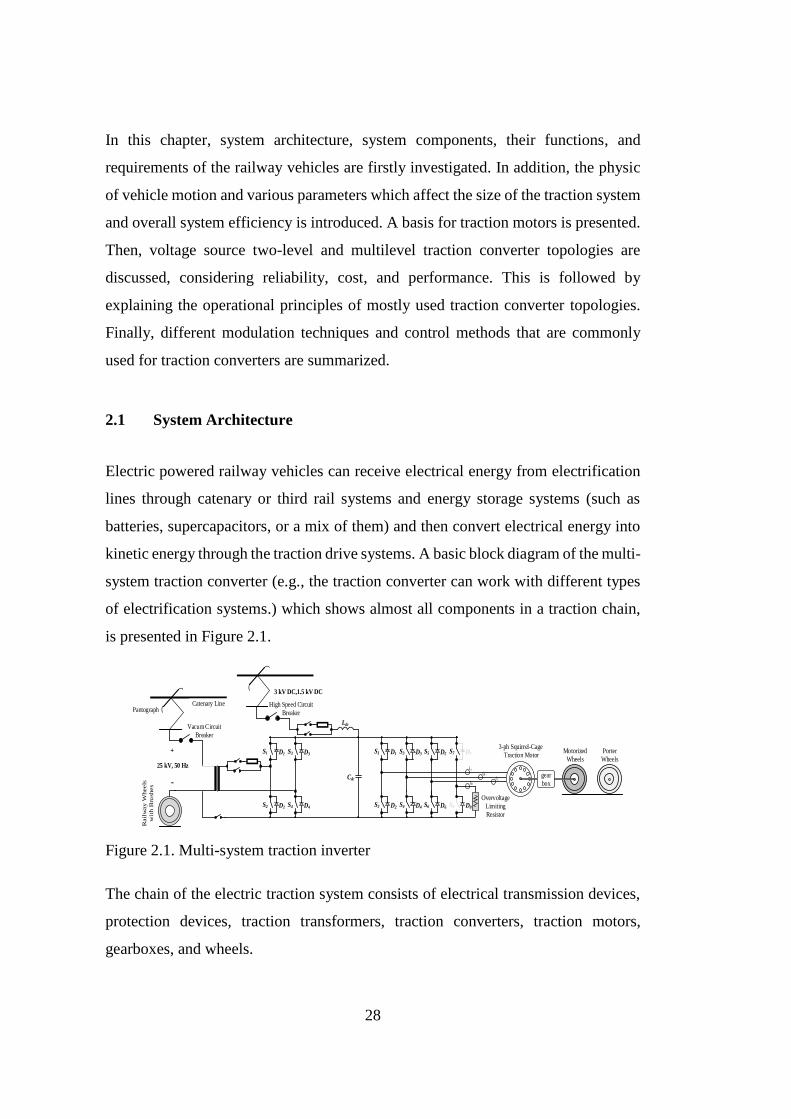
28

In this chapter, system architecture, system components, their functions, and

requirements of the railway vehicles are firstly investigated. In addition, the physic

of vehicle motion and various parameters which affect the size of the traction system

and overall system efficiency is introduced. A basis for traction motors is presented.

Then, voltage source two-level and multilevel traction converter topologies are

discussed, considering reliability, cost, and performance. This is followed by

explaining the operational principles of mostly used traction converter topologies.

Finally, different modulation techniques and control methods that are commonly

used for traction converters are summarized.

2.1 System Architecture

Electric powered railway vehicles can receive electrical energy from electrification

lines through catenary or third rail systems and energy storage systems (such as

batteries, supercapacitors, or a mix of them) and then convert electrical energy into

kinetic energy through the traction drive systems. A basic block diagram of the multi-

system traction converter (e.g., the traction converter can work with different types

of electrification systems.) which shows almost all components in a traction chain,

is presented in Figure 2.1.

S1 D1 S3 D3

S2 D2 S4 D4

iA

Overvoltage

Limiting

Resistor

3-ph Squirrel-Cage

Traction MotorS1

Cdc

Ldc

D1 Motorized

Wheels

gear

box

S3 D3 S5 D5

S2 D2 S4 D4 S6 D6 S8 D8

Porter

WheelsS7 D7

iB

iC

iR

+

-

Catenary Line

Rail

way

Wheels

wit

h B

rush

es

25 kV, 50 Hz

Vacum Circuit

Breaker

PantographHigh Speed Circuit

Breaker

3 kV DC,1.5 kV DC

Figure 2.1. Multi-system traction inverter

The chain of the electric traction system consists of electrical transmission devices,

protection devices, traction transformers, traction converters, traction motors,

gearboxes, and wheels.

29

Pantograph or third rail brush draws energy from the power line. Depending on the

types of electrification system, the energy first feeds the traction transformer (for AC

fed converters) or directly to input filters of the traction inverter (for DC line fed

converters). In fact, the traction converter with its superior control algorithms and

functions is the core of the traction system. It acts as the heart of the traction system.

It takes electrical energy and synthesizes required current and voltage waveforms for

the traction motors to move trains. The traction motor acts as a muscle in the human

body. It converts electrical energy to kinetic energy. Mechanical energy is

transferred to the wheels via the gearbox.

Traction converters have direct or indirect interfaces with many system components,

including different engineering disciplines such as vehicle control computers,

traction transformers, traction motors, encoders, protection devices on railway

vehicles, and electrification lines. It is worthy to note that the types of energy sources

and the voltage level have a strong effect on the design of traction converters.

The types of railway electrification systems are defined in Chapter 1. According to

applications, AC/DC electrification lines with different voltage levels are used in

different countries. The choice of energy sources is strictly dependent on vehicle

requirements. Low voltage DC electrification systems (750 VDC and 1500 VDC)

and batteries/supercapacitors are commonly used for metro and light rail vehicles,

which require higher acceleration/deceleration rates and frequent starting-stopping.

In other words, low voltage electrifications are more common for shorter distances

and low power applications. When the rail vehicles are supplied with DC, there is no

need to perform AC/DC conversion at the input stage of the traction converter; DC

input of the traction converter can be directly fed from the DC electrification line.

DC fed systems mainly consist of traction inverters, traction motors, gearboxes,

protection equipment such as high-speed circuit breakers (HSCB), surge arrestors,

fuses, braking choppers [24]. These systems do not contain big and heavy power

transformers. Thus, the traction system chains are cheaper and lighter. On the other

hand, 3000 VDC and 15/25 kVAC electrification systems are mostly used for long

distances and high power trains such as regional trains, very high-speed/high-speed

30

trains, and mainline locomotives. Unlike the DC-fed traction systems, AC-fed

traction systems need an AC/DC conversion stage at the input stage of the traction

inverter. Therefore, input (line) converters and traction transformers are additionally

used in AC-fed traction systems.

In summary, the main requirements of a traction system can be defined according to

the following constraints:

Electrification system specification

Vehicle specifications (e.g., empty weight, payload capacity, type, etc.)

Drive cycle and special requirements (e.g., acceleration and deceleration

rates, maximum speed, etc.)

Track profile (e.g., distances, grades, curves, etc.)

Network management (e.g., number of vehicles in operation)

2.1.1 Functions of Traction System Components

The main components of traction systems are summarized under the following

topics:

1) Pantograph or Third Rail Brush:

There are two different types of contact to transmit the electrical energy to railway

vehicles, namely third rail contact or catenary contact. The third rail contact systems

are located on the ground. Hence, this type of contact has to be protected to avoid

injury, dead or electric shocks of people. Because of that reason, this type of contact

is mostly used for underground vehicles at low voltage levels such as 600 VDC or

750 VDC. The most important advantage of the third rail contact is that it allows

tunnel diameters to be opened small and consequently reduces tunneling cost. On the

other hand, due to safety reasons, above 1000 V, catenary type contacts are used to

31

feed traction systems of trains. Third rail brushes are used in third rail contact

systems, whereas pantographs are used in the catenary contact systems.

A pantograph or a third rail brush is an electro-mechanical device. The electrical

energy is supplied through the pantographs or the third rail brushes to the rail vehicle

from the electrification system (catenary or third rail) during the working time of the

vehicle. Thus, these electro-mechanical devices have to maintain good electric

contact under all running speed conditions. Because of the increasing ground

disturbances with speed, it is difficult to provide good electrical contact. Springs or

air pressure is used to ensure good electrical contact between the electrification line

and the pantograph or third rail brush [24].

2) Surge Arrester:

A surge arrester is a device to protect electrical equipment from overvoltage

transients that can be caused by external (lightning) or internal (switching) events.

The surge arrester should be connected between the transmission line and the ground

in front of the other protective devices such as circuit breakers (both sides of the

circuit breaker should be considered) to protect all electrical equipment against

overvoltage transients. A surge arrestor should have a low impulse ratio to provide a

fast response time [24].

3) DC or AC Circuit Breaker:

DC or AC circuit breaker is a protection device to be used for safely interrupting

high currents that are caused by an electrical failure of the power system components

during the operation of a train. The response time of the circuit breaker is very

important. Faster response time reduces the effect of short circuit stress on traction

transformers, traction converters, traction motors, insulators, and cables/conductors

[24], [50].

32

4) Traction Transformer:

Traction transformers are used to step down the AC catenary voltage to safe voltage

levels to transmit on the vehicles and appropriate voltage levels for traction

converters. There are two different solutions. The first and oldest one is a single-

phase low frequency (162/3 Hz or 50 Hz or 60 Hz) traction transformer. It usually

steps down the 15 kV or 25 kV catenary voltage to traction converter operating

voltage in the range of 800 V – 2000 V. Traction converters that fed on AC catenary

line, mainly composed of a four-quadrant single-phase line rectifier and a four-

quadrant three-phase inverter. The single-phase line rectifier takes AC input voltage

and converts it to DC voltage while it is operating almost unity power factor.

There are also some limitations on catenary current harmonics. If the transformer

leakage inductances are sufficient to keep harmonics below the required limits with

the help of converter modulation methods, there is no need to use an additional input

filter at the traction converter input. Otherwise, it will be necessary to use an

additional input filter at the transformer and/or (typically a line reactor) at the

converter input. Moreover, for the high power levels (e.g., 1 MVA or above), 100

Hz voltage ripple is so strong on DC link voltage. In order to filter it, second-order

tuned filters are used in high-power applications. This filter is composed of a main

capacitance block and a reactor. This reactor is mostly embedded in the traction

transformer due to the high cooling requirement.

It is worthy to note that the second and innovative solution is to use medium

frequency (several kHz) traction transformers. The catenary voltage directly feeds to

the cascaded H-bridge multilevel rectifier. The output of each H-bridge converter is

connected to a resonant converter and medium frequency traction transformer. Thus,

the transformer volume and weight can be reduced considerably due to the medium

frequency switching operation. Although there are some examples of medium-

frequency traction transformers for 15 kV/162/3 Hz electrification, this solution has

not become widespread. Due to the breakdown voltages of existing IGBTs, many H-

bridge converters have to be connected in series. This situation decreases the benefits

33

that can be achieved with medium frequency transformers such as lightweight, low

volume, high efficiency, and reliability. It is considered that this solution can become

widespread with the high breakdown voltages that can be reached by state-of-the-art

SiC semiconductors [24], [51].

5) Traction Converter:

Traction converters are responsible for vehicle motion. They take electrical energy

from electrification systems (AC or DC systems) and generate appropriate voltage

and current waveforms to drive traction motors. The traction converter design varies

according to the electrification system. For AC fed traction converters, two main

types of power converters are located in the traction converter box, such as a four-

quadrant single-phase line rectifier and a three-phase inverter. For DC fed traction

converters, there is only an inverter power block as the main part. Since the traction

converters are examined in detail within the scope of the thesis, this part was kept

simple [51].

6) Brake System:

Brake systems can be specified as the most important subsystem of a railway vehicle

in terms of safety. In railway applications, the brake systems are categorized under

two main groups, namely as adhesion brake systems and non-adhesion brake

systems. Mechanical brakes and electric brakes are located under the adhesion type

brake systems, while air resistance brakes and electro-magnetic rail brakes are in

non-adhesion type brake systems. Adhesion-type brake systems have utilized the

friction between the rail and wheel. During rain and snow, the friction coefficient

between the rail and wheel decreases, and dirty/iced/wet rails make it impossible to

apply strong braking force. If the brake force is too high for those rail conditions, the

wheels start to slide. This situation makes the drive systems unsafe by prolonging

the stopping distance and negatively affecting vehicle dynamics. It can also damage

the wheels by disrupting the surface of the wheel. In order to prevent this situation,

wheel slide protection systems are used for both mechanical brakes and electric

34

brakes by utilizing sanding. They detect the wheel slide and reduce the applied

braking force. Besides this, the non-adhesion type brake systems do not use friction

between the rail and the wheel. Hence, in some railway applications, especially in

tramways and high-speed trains, the electro-magnetic rail brake systems are also

preferred in addition to the adhesion type brake system to increase the drive system

safety and decrease the stopping distance under unexpected conditions [52].

7) Energy Storage System:

The energy consumption of trains depends on drive cycles, vehicle speed, vehicle

volume, vehicle weight, the efficiency of power converters, energy recovery ability,

electrification systems, and track profiles. Especially, vehicle weight depends on the

material (e.g., aluminum or steel) of car bodies, the weight of traction system

components, auxiliary power converters, air conditioning power unit, and passenger

capacity [24]. In order to decrease energy consumption, important attempts have

been made to reduce vehicle weights. Aluminum-made bodies are used to decrease

vehicle mass. In addition to this, with the help of newly developed technological

power semiconductors, the size and weight of the traction converters and auxiliary

power converters are further reduced [21]. The energy efficiency of power converters

is also improved together with the weight and size reduction. These improvements

contribute to the reduction of energy consumption. Besides this, network

management and drive cycle strategies, together with modern electrification systems,

also make a great contribution to reducing energy consumption. Because, during the

braking process, most of the energy is still lost as heat on the braking resistors to

prevent an overvoltage on the catenary for DC fed traction systems. If this braking

energy can be delivered to the other vehicles operated at the same network or

delivered back to the mains, a great amount of braking energy will be recovered.

Another way to recover braking energy is the use of energy storage systems. If

energy storage systems are used on the vehicle or at power substations, a great

portion of the regenerative energy can be recovered. This stored energy can further

35

help to reduce energy consumption and improve catenary line regulation when it is

used at the instant of acceleration process of the vehicle.

Figure 2.2 shows a classification of existing energy storage technologies considering

the power and energy densities [53].

Figure 2.2. Ragone chart of energy density vs. power density of different energy

storage devices [53]

In fact, the braking times are usually less than 30 seconds for metro and light rail

vehicles. However, peak power levels are very high in this time interval. Therefore,

the energy storage technologies to be used in the recovery of the braking energy must

accordingly have a high power density. Besides this, there may also be a need for

different energy storage technologies that require high energy density in applications

where catenary free operation is required. Moreover, both specifications are needed

together in some applications due to the high power and high-energy requirements.

Ragone's chart shows that supercapacitors fit quite well for these requirements.

8) Braking Chopper & Braking Resistor:

There are two types of electric (or dynamic) braking, namely, regenerative braking

and rheostatic braking. During dynamic braking, the traction motors are used as a

generator. If the generated electrical energy is returned to the electrification system,

it is called regenerative braking, and if the generated electrical energy is dissipated

as heat in a resistor, it is called rheostatic braking. For both cases, incoming electrical

36

energy charges the DC-link capacitors and causes a voltage rise at the DC-link

voltage. If the DC-link voltage reaches a very high value (e.g., comparable levels

with breakdown voltages) during the dynamic braking, the power semiconductors

and DC-link capacitors will be damaged [24].

For the DC fed traction systems, the line voltage increases at the braking instant due

to the nature of diode bridge rectifier-based electrification systems. Some or all of

the generated energy can be used by the other railway vehicles if the working

conditions are fully appropriate. However, this state will not be possible most of the

time. In order to control DC-link voltage, electrical energy can be sent to the

electrification system, be stored in energy storage systems, and be burnt in onboard

braking resistors with the help of braking choppers [54]. Generally, for AC-fed

traction systems, braking resistors and choppers are not used due to the bidirectional

power flow nature of AC electrification systems.

9) Traction Motor:

The main components which are used to convert electrical energy to kinetic energy

are traction motors. Traction motors provide the required mechanical propulsion for

the train. Traction motors are usually located in the bogie in order to minimize

mechanical transmission needs and transmission losses. However, this also brings

some difficulties together. Actually, there is not a big space for mounting the traction

motors on the bogie. Because of this reason, power to volume ratios of traction

motors are so strict. In the past, DC traction motors were used in railway systems.

Nowadays, squirrel cage induction motors and permanent magnet synchronous

motors are used in railway systems. These traction motors have superior advantages

in terms of power to volume and power to weight ratio and low maintenance

requirements. Nowadays, between these two traction motors, the squirrel cage

induction motors are commonly used. The permanent magnet synchronous motors

have not been spread yet in railway systems, although they are the most

advantageous in terms of the properties mentioned above. Besides this, there are

some special applications in which the permanent magnet synchronous motors are

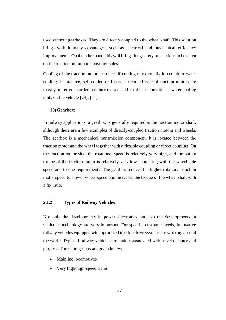
37

used without gearboxes. They are directly coupled to the wheel shaft. This solution

brings with it many advantages, such as electrical and mechanical efficiency

improvements. On the other hand, this will bring along safety precautions to be taken

on the traction motor and converter sides.

Cooling of the traction motors can be self-cooling or externally forced air or water

cooling. In practice, self-cooled or forced air-cooled type of traction motors are

mostly preferred in order to reduce extra need for infrastructure like as water cooling

units on the vehicle [24], [51].

10) Gearbox:

In railway applications, a gearbox is generally required at the traction motor shaft,

although there are a few examples of directly-coupled traction motors and wheels.

The gearbox is a mechanical transmission component. It is located between the

traction motor and the wheel together with a flexible coupling or direct coupling. On

the traction motor side, the rotational speed is relatively very high, and the output

torque of the traction motor is relatively very low comparing with the wheel side

speed and torque requirements. The gearbox reduces the higher rotational traction

motor speed to slower wheel speed and increases the torque of the wheel shaft with

a fix ratio.

2.1.2 Types of Railway Vehicles

Not only the developments in power electronics but also the developments in

vehicular technology are very important. For specific customer needs, innovative

railway vehicles equipped with optimized traction drive systems are working around

the world. Types of railway vehicles are mainly associated with travel distance and

purpose. The main groups are given below:

Mainline locomotives

Very high/high-speed trains

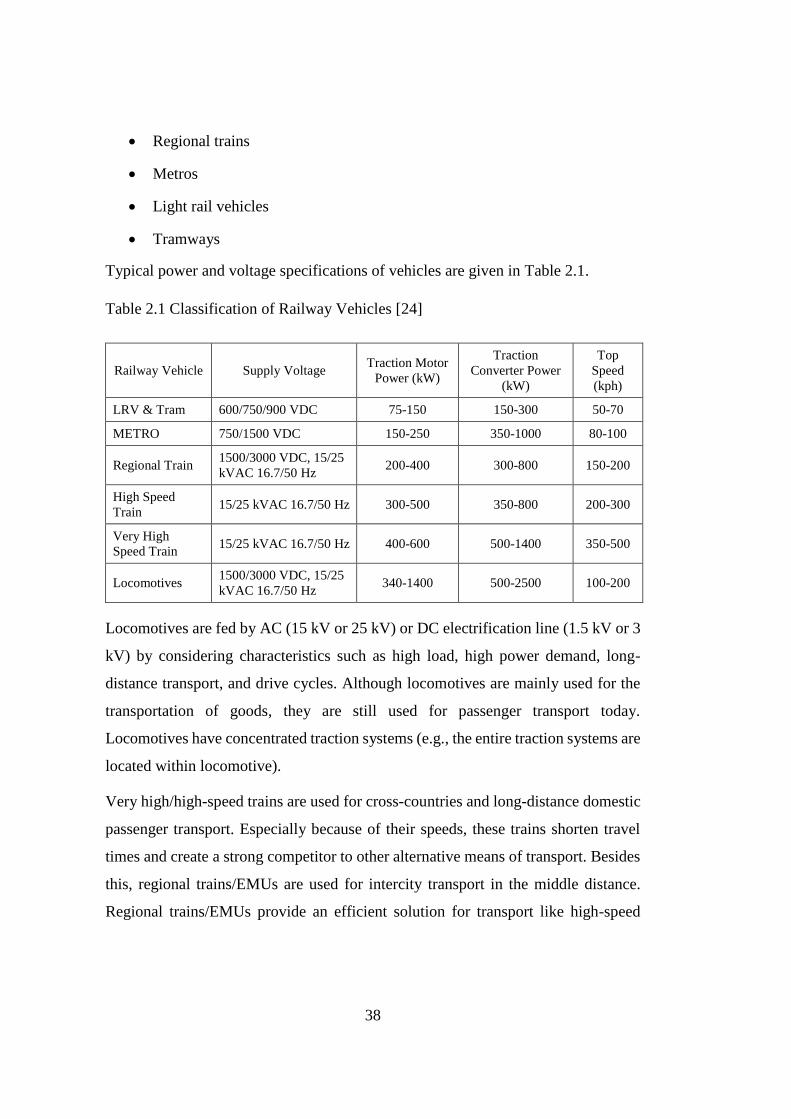
38

Regional trains

Metros

Light rail vehicles

Tramways

Typical power and voltage specifications of vehicles are given in Table 2.1.

Table 2.1 Classification of Railway Vehicles [24]

Railway Vehicle Supply Voltage Traction Motor

Power (kW)

Traction

Converter Power

(kW)

Top

Speed

(kph)

LRV & Tram 600/750/900 VDC 75-150 150-300 50-70

METRO 750/1500 VDC 150-250 350-1000 80-100

Regional Train 1500/3000 VDC, 15/25

kVAC 16.7/50 Hz 200-400 300-800 150-200

High Speed

Train 15/25 kVAC 16.7/50 Hz 300-500 350-800 200-300

Very High

Speed Train 15/25 kVAC 16.7/50 Hz 400-600 500-1400 350-500

Locomotives 1500/3000 VDC, 15/25

kVAC 16.7/50 Hz 340-1400 500-2500 100-200

Locomotives are fed by AC (15 kV or 25 kV) or DC electrification line (1.5 kV or 3

kV) by considering characteristics such as high load, high power demand, long-

distance transport, and drive cycles. Although locomotives are mainly used for the

transportation of goods, they are still used for passenger transport today.

Locomotives have concentrated traction systems (e.g., the entire traction systems are

located within locomotive).

Very high/high-speed trains are used for cross-countries and long-distance domestic

passenger transport. Especially because of their speeds, these trains shorten travel

times and create a strong competitor to other alternative means of transport. Besides

this, regional trains/EMUs are used for intercity transport in the middle distance.

Regional trains/EMUs provide an efficient solution for transport like high-speed

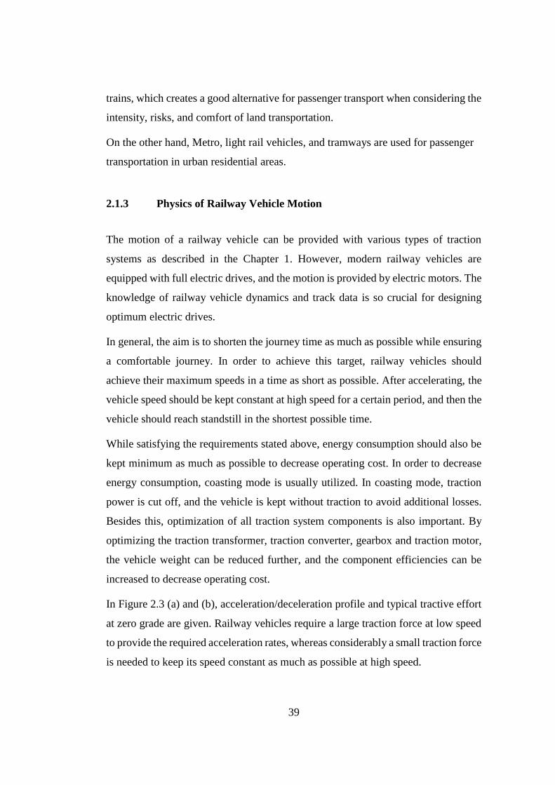
39

trains, which creates a good alternative for passenger transport when considering the

intensity, risks, and comfort of land transportation.

On the other hand, Metro, light rail vehicles, and tramways are used for passenger

transportation in urban residential areas.

2.1.3 Physics of Railway Vehicle Motion

The motion of a railway vehicle can be provided with various types of traction

systems as described in the Chapter 1. However, modern railway vehicles are

equipped with full electric drives, and the motion is provided by electric motors. The

knowledge of railway vehicle dynamics and track data is so crucial for designing

optimum electric drives.

In general, the aim is to shorten the journey time as much as possible while ensuring

a comfortable journey. In order to achieve this target, railway vehicles should

achieve their maximum speeds in a time as short as possible. After accelerating, the

vehicle speed should be kept constant at high speed for a certain period, and then the

vehicle should reach standstill in the shortest possible time.

While satisfying the requirements stated above, energy consumption should also be

kept minimum as much as possible to decrease operating cost. In order to decrease

energy consumption, coasting mode is usually utilized. In coasting mode, traction

power is cut off, and the vehicle is kept without traction to avoid additional losses.

Besides this, optimization of all traction system components is also important. By

optimizing the traction transformer, traction converter, gearbox and traction motor,

the vehicle weight can be reduced further, and the component efficiencies can be

increased to decrease operating cost.

In Figure 2.3 (a) and (b), acceleration/deceleration profile and typical tractive effort

at zero grade are given. Railway vehicles require a large traction force at low speed

to provide the required acceleration rates, whereas considerably a small traction force

is needed to keep its speed constant as much as possible at high speed.

40

There are four operating regions of vehicle movement, namely acceleration, constant

speed operation, coasting, and braking. These areas can be visualized in Figure 2.3. V

ehic

le S

pee

d (k

m/h

)Tr

acti

on

Forc

e (k

N)

Time,s

(a)

(b)

Acc

eler

atio

n w

ith

co

nsta

nt

torq

ue

Acc

eler

atio

n w

ith

co

nsta

nt

po

wer

Coa

stin

g

Con

stan

t sp

eed

Bra

kin

g w

ith

max

imu

m

dec

eler

atio

n

Acc

eler

atio

n

Con

stan

t sp

eed

Coa

stin

g

Bra

kin

g

A

B C D

E

Figure 2.3. Typical acceleration and deceleration profile of a light rail vehicle

Practically, the shape of the speed-time curve of vehicles may be different than

shown in Figure 2.3 because of the gradients, curvatures, and speed limits. However,

this figure is good enough to explain operating regions. Four different operation

regions are seen in the figure: acceleration period from A to B, constant speed period

from B to C, coasting (free-running) period from C to D, and the braking period from

D to E. The understanding of railway vehicle motion is very important to define the

optimum traction system requirements. Because fully defined system models make

it possible to accurately derive the traction system requirements. Therefore, the

wheel-rail contact relation, the vehicle model and train resistance, track profile, and

electrification system properties should also be well known.

1) Wheel-Rail Contact Relation

Traction motors convert electrical energy to mechanical energy and deliver it to the

wheels via the gearbox. A considerable amount of torque is generated at the wheel

shaft. However, the applied torque that can be transmitted from the wheels to the rail

41

is limited by adhesion force which is the transmitted tangential force in the

longitudinal direction between the rail and wheels [55]. Low adhesion can limit the

transmittable torque to a considerable level. The difference between the applied force

and counter forces (e.g., train resistance and gravitational force) are used to

accelerate or decelerate the train.

w

T

r

θ

m.g.sin(θ)

Figure 2.4. Forces acting on the rail

The 𝐹𝑁 is the normal force acting on the rail. 𝐹𝑇 is the tangential force which is also

known as adhesion force. The ratio between the adhesion force and normal force is

known as the adhesion coefficient, 𝜇0 [55].

𝐹𝑁 = 𝑚𝑔𝑠𝑖𝑛(𝜃)𝜇0 (2-1)

𝜇0 = 𝐹𝑇/𝐹𝑁 (2-2)

If this ratio is so small, the transmittable torque is strictly limited, and undesirable

slip and slide conditions may occur.

The maximum transmittable torque, 𝑇𝑇 can be calculated as follows.

𝐹𝑇 ≤ 𝑚𝑔𝑠𝑖𝑛(𝜃)𝜇0 (2-3)

𝑇𝑇 ≤ 𝑚𝑔𝑠𝑖𝑛(𝜃)𝜇0𝑟 (2-4)

During the operation of a railway vehicle, the maximum torque should be limited

according to these constraints; otherwise, the wheel will tend to slip or slide

depending on the operation phase (e.g., acceleration or deceleration) [55].

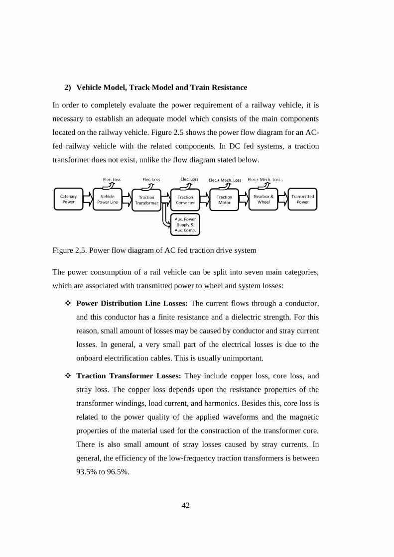
42

2) Vehicle Model, Track Model and Train Resistance

In order to completely evaluate the power requirement of a railway vehicle, it is

necessary to establish an adequate model which consists of the main components

located on the railway vehicle. Figure 2.5 shows the power flow diagram for an AC-

fed railway vehicle with the related components. In DC fed systems, a traction

transformer does not exist, unlike the flow diagram stated below.

Catenary Power

Vehicle Power Line

Elec. Loss

Traction Transformer

Elec. Loss

Traction Converter

Elec. Loss

Traction Motor

Elec.+ Mech. Loss

Gearbox & Wheel

Elec.+ Mech. Loss

Transmitted Power

Aux. Power Supply &

Aux. Comp.

Figure 2.5. Power flow diagram of AC fed traction drive system

The power consumption of a rail vehicle can be split into seven main categories,

which are associated with transmitted power to wheel and system losses:

Power Distribution Line Losses: The current flows through a conductor,

and this conductor has a finite resistance and a dielectric strength. For this

reason, small amount of losses may be caused by conductor and stray current

losses. In general, a very small part of the electrical losses is due to the

onboard electrification cables. This is usually unimportant.

Traction Transformer Losses: They include copper loss, core loss, and

stray loss. The copper loss depends upon the resistance properties of the

transformer windings, load current, and harmonics. Besides this, core loss is

related to the power quality of the applied waveforms and the magnetic

properties of the material used for the construction of the transformer core.

There is also small amount of stray losses caused by stray currents. In

general, the efficiency of the low-frequency traction transformers is between

93.5% to 96.5%.

43

Traction Converter Losses: Converter losses include copper loss (bus bars,

filters, cables and etc.), power semiconductor loss (e.g., switching and

conduction), and stray current loss. A considerable part of the inverter losses

may arise from power semiconductors and line reactor losses. In general, the

efficiencies of IGBT-based traction converters are between 95% to 98%.

Nowadays, the converter efficiencies can be improved with SiC power

semiconductors over 99%.

Auxiliary Power Supply and Auxiliary Component Losses: They include

copper loss (bus bars, filters and etc.), power semiconductor loss (e.g.,

switching and conduction), reactive component loss, stray current loss, and

auxiliary component losses for passenger comfort such as fans, cooling

systems, heating and lighting systems, toilets, and etc.

Traction Motor Losses: It is well known that the losses in a traction machine

include stator and rotor copper losses, core loss, friction, and windage loss,

and stray current loss. Nowadays, the squirrel cage induction motors are

widely used in railway applications, and their efficiencies are usually

between 92% to 94%. The traction motor efficiency can be increased up to

97% by using permanent magnet synchronous motors [56].

Mechanical Losses: Traction motor output torque has to overcome the total

load caused by gearbox friction, train resistance, curvature resistance of rails,

gravitational forces in order to accelerate railway vehicles. The gravitational

force is proportional to the instantaneous vehicle mass. The energy invested

for the acceleration of a railway vehicle or uphill driving does not directly

cause a considerable amount of losses. A large portion of the energy can be

restored in the energy storage systems or transmitted back to the

electrification line except for the copper, electro-magnetic and mechanical

losses. If this energy is not stored or transmitted, it may be dissipated as heat

on the braking resistor or mechanical brake. By the way, gearbox loss, train,

and curvature resistances directly create unrecoverable power losses.

44

Transmitted Power: The transmitted power from the wheel to rail is used to

control the speed of the railway vehicle.

The losses, resistances, and counter forces mentioned above always oppose the

vehicle movement except for gravitational force, 𝐹𝑔𝑟𝑣. In areas where the slope is

negative, the gravitational force acts in the direction of supporting the movement of

the vehicle. Where it is positive, the opposite is valid. The effect of these forces on

the train is represented in equation (2-5).

𝐹𝑎𝑝𝑝𝑙𝑖𝑒𝑑 − 𝐹𝑒𝑥𝑡 = 𝑚𝑒𝑎 (2-5)

where 𝑚𝑒 is the equivalent mass of the train, which contains the static mass of the

train 𝑚 and the reflected mass from the inertias of wheels, gearboxes, motors,

couplings, axles and etc.

The external acting forces can be written as in equation (2-6).

𝐹𝑒𝑥𝑡 = 𝐹𝑡𝑟 + 𝐹𝑖𝑠 + 𝐹𝑔𝑟𝑣 + 𝐹𝑐𝑢𝑟𝑣𝑒 (2-6)

where 𝐹𝑡𝑟 is the sum of static and dynamic resistances and drag force acting on the

vehicle, 𝐹𝑖𝑠 is the initial static force of the vehicle system, which is dominant at

starting instant and at very low speeds, 𝐹𝑔𝑟𝑣 is the gravitational force caused by the

land slope, 𝐹𝑐𝑢𝑟𝑣𝑒 is the force countered by the curve resistance as stated in equation

(2-7).

𝐹𝑐𝑢𝑟𝑣𝑒 = 𝐷𝑀𝑔/𝑅(𝑥) (2-7)

where, 𝐷 curve resistance coefficient, and 𝑅 is the radius of any curve on the rail

track.

The formula for train resistance is given equation (2-8) which is known as Davis

Equation. Theoretical calculation of these coefficients is very difficult. These

coefficients are usually determined by experimental tests [57].

45

𝐹𝑡𝑟 = 𝐴𝑚 + 𝐵𝑣𝑚 + 𝐶𝑣2 (2-8)

In (2-8), 𝐴 is the friction force coefficient per unit weight of the vehicle which is

independent of speed, 𝐵 is a constant per unit weight of the vehicle to give dynamic

friction force proportional to speed, 𝐶 is the air resistance coefficient when

multiplied by the square of the speed gives the aerodynamic drag force acting on the

vehicle. Figure 2.6 shows some illustrative examples of train resistances at the half

and full load conditions [24].

Trai

n R

esis

tan

ce (

kN)

Vehicle Speed, km/h

with full passenger load

with half passenger load

Figure 2.6. Typical train resistance of a light rail vehicle

On the other hand, 𝐹𝑔𝑟𝑣 gravitational force is as given in equation (2-9).

𝐹𝑔𝑟𝑣 = 𝑚𝑔𝑠𝑖𝑛(𝜃) (2-9)

A complete mathematical model of a public transportation vehicle running on a

specific rail track is given in this section. The force–balance equation on the

translational motion side is given in (2-10).

𝑚𝐹𝑠ℎ𝑎𝑓𝑡 = 𝑀𝑒𝑞𝑣

𝑑𝑣

𝑑𝑡 + [𝐹𝑟 + 𝐹𝑐𝑢𝑟𝑣𝑒 +𝑀𝑔𝑠𝑖𝑛[𝛼(𝑥)]] (2-10)

where, m is the number of traction motors, 𝐹𝑠ℎ𝑎𝑓𝑡 the tractive force per motor

reflected to the translational motion side by assuming rigid shafts, 𝑀𝑒𝑞𝑣 the mass of

static and rotating parts of transportation vehicle excluding motor inertias, v the

46

linear speed of the vehicle, 𝐹𝑟 the sum of static and dynamic resistances and drag

force acting on the vehicle, 𝐹𝑐𝑢𝑟𝑣𝑒 the curve resistance force, 𝑀 the static mass of the

vehicle, 𝑔 the gravitational acceleration, and 𝛼 the slope angle of the rail track as a

function of displacement, 𝑥 from a reference point. 𝑀𝑒𝑞𝑣 in (2-10) has three

components as given in (2-11).

𝑀𝑒𝑞𝑣 = 𝑀 + 𝐽𝑔𝑏

1

𝑟2+ 𝐽𝑤

1

𝑟2 (2-11)

where, 𝐽𝑔𝑏 and 𝐽𝑤 are respectively moment of inertia of all gear-boxes and wheels

on the low rotational speed side. Equation (2-10) can be referred to the motor shaft

by substituting 𝑣 = 𝜔𝑟/𝑛 and dividing both sides by gear down ratio, 𝑛, and m.

These yields (2-12)

[𝐽𝑚 + (𝑀𝑒𝑞𝑣𝑟

2

𝑚𝑛2)]

𝑑𝜔

𝑑𝑡= 𝑇𝑚 −

1

𝑚[𝑇𝑟 + 𝑇𝑐𝑢𝑟𝑣𝑒 + (

𝑀𝑔𝑟

𝑛) 𝑠𝑖𝑛[𝛼(𝑥)]] (2-12)

where, 𝐽𝑚 is the motor inertia in kg-m2, 𝜔 is the motor speed in mech-rad/s, 𝑇𝑚 is

the torque output of each traction motor in Nm, 𝑟 the radius of the wheels in m, and

𝑇𝑟 and 𝑇𝑐𝑢𝑟𝑣𝑒 are the load torque components owing to the train resistance and the

curve resistance of the rail track, respectively.

𝑇𝑟 and 𝑇𝑐𝑢𝑟𝑣𝑒 are expressed as given in (2-13) and (2-14).

𝑇𝑟 = [(𝐴 + 𝐵𝑣) 𝑀 + 𝐶𝑣2 ] 𝑟/𝑛 (2-13)

𝑇𝑐𝑢𝑟𝑣𝑒 = (𝐷𝑀𝑔/𝑅(𝑥)) 𝑟/𝑛 (2-14)

3) Train Duty-Cycle and Electrification System

In railway applications, as mentioned before, there is not much free space on the

bogie to integrate the traction motors. In addition, the component masses and sizes

should be minimized in order to decrease mechanical losses and improve the

system's overall efficiency. The development of an optimized traction system for a

given application involves a complex, iterative process to decide the number of

traction motors, motor size, inverter rated power, cooling system, etc. [58]. For this

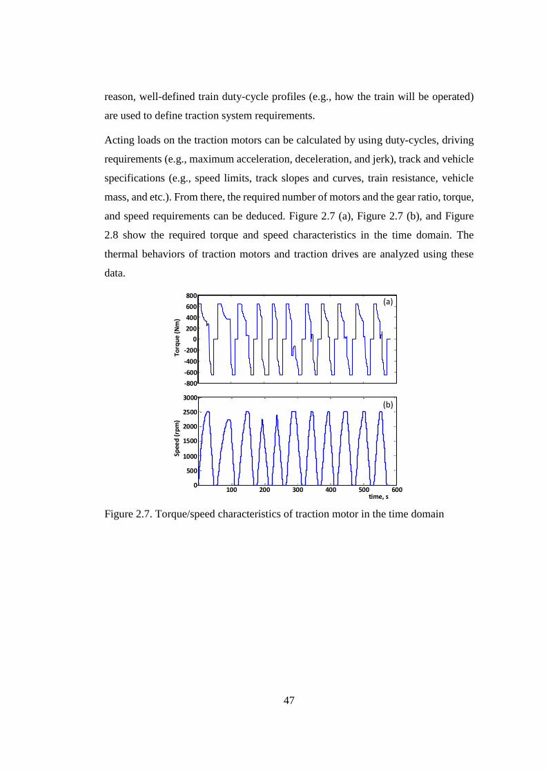
47

reason, well-defined train duty-cycle profiles (e.g., how the train will be operated)

are used to define traction system requirements.

Acting loads on the traction motors can be calculated by using duty-cycles, driving

requirements (e.g., maximum acceleration, deceleration, and jerk), track and vehicle

specifications (e.g., speed limits, track slopes and curves, train resistance, vehicle

mass, and etc.). From there, the required number of motors and the gear ratio, torque,

and speed requirements can be deduced. Figure 2.7 (a), Figure 2.7 (b), and Figure

2.8 show the required torque and speed characteristics in the time domain. The

thermal behaviors of traction motors and traction drives are analyzed using these

data.

0 100 200 300 400 500 600

0 100 200 300 400 500 6000

500

1000

1500

2000

2500

3000

Spee

d (

rpm

)To

rqu

e (N

m)

2500

3000

2000

1500

1000

500

0

0

200

400

600

800

-200

-400

-600

-800

time, s100 200 300 400 500 600

(a)

(b)

Figure 2.7. Torque/speed characteristics of traction motor in the time domain

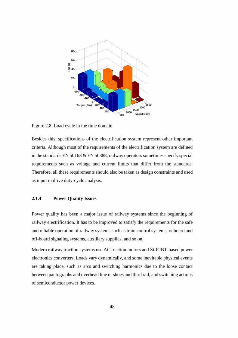
48

12

34

5

1

23

45

6

7

0

20

40

60

80

Detached Style

5001000

15002000

25000

200400

600

-200-400

-600

0

20

40

60

80

Speed (rpm)

Torque (Nm)

Tim

e (s

)

Figure 2.8. Load cycle in the time domain

Besides this, specifications of the electrification system represent other important

criteria. Although most of the requirements of the electrification system are defined

in the standards EN 50163 & EN 50388, railway operators sometimes specify special

requirements such as voltage and current limits that differ from the standards.

Therefore, all these requirements should also be taken as design constraints and used

as input in drive duty-cycle analysis.

2.1.4 Power Quality Issues

Power quality has been a major issue of railway systems since the beginning of

railway electrification. It has to be improved to satisfy the requirements for the safe

and reliable operation of railway systems such as train control systems, onboard and

off-board signaling systems, auxiliary supplies, and so on.

Modern railway traction systems use AC traction motors and Si-IGBT-based power

electronics converters. Loads vary dynamically, and some inevitable physical events

are taking place, such as arcs and switching harmonics due to the loose contact

between pantographs and overhead line or shoes and third rail, and switching actions

of semiconductor power devices.

49

Urban traction systems use DC electrification systems which mostly consist of 12-

pulse diode rectifiers. These systems generate high amount of harmonics on the grid

side. Especially, the orders of the highest current harmonics are 11th and 13th. In

addition to this, the AC and DC fed traction systems also produce relatively high-

frequency harmonics due to the switching operation of the power semiconductors.

In the literature, many studies have been conducted to improve the power quality of

railway electric networks. Most of these studies are related to compensation

strategies that are used to make power quality better at the electrification network

side. Only a few of them deal with the traction load side improvements [59].

However, the presence of harmonic components created from traction systems can

cause faulty train management by disturbing signaling and communication systems.

Recently used methods for load side harmonic reduction are improving the

modulation methods of traction converters, use of passive filtering components,

and/or multilevel power converter topologies. Especially as the switching frequency

increases, the control capabilities of the power electronics converters also increase.

However, because of the huge semiconductor losses, the switching frequency of the

power electronics converters could not be increased. This deficiency was eliminated

with the discovery of multilevel converters. Thus, differential and common noises

are reduced. There are also some other benefits featured with the use of multilevel

converters that decrease the stresses on transformer and motor winding insulations,

semiconductor devices, and bearing currents.

On the other hand, SiC MOSFET technology, which is becoming widespread today,

offers many benefits to increase capabilities of power electronics converters and

make control of power converters easy and better by eliminating the need for some

special modulation methods such as SHEPWM, SHMPWM, and OPWM. Switching

frequencies of medium voltage and medium power converters can be increased 5 to

15 times as compared to the latest Si-IGBT-based power electronics converters. As

a result of this, the control bandwidths and harmonics have been remarkably

improved. As opposed to this, common-mode noises are increased due to the fast

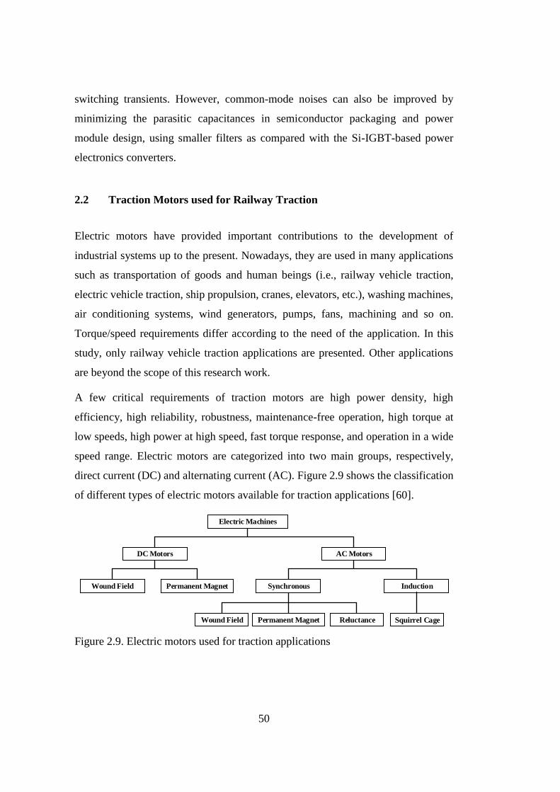
50

switching transients. However, common-mode noises can also be improved by

minimizing the parasitic capacitances in semiconductor packaging and power

module design, using smaller filters as compared with the Si-IGBT-based power

electronics converters.

2.2 Traction Motors used for Railway Traction

Electric motors have provided important contributions to the development of

industrial systems up to the present. Nowadays, they are used in many applications

such as transportation of goods and human beings (i.e., railway vehicle traction,

electric vehicle traction, ship propulsion, cranes, elevators, etc.), washing machines,

air conditioning systems, wind generators, pumps, fans, machining and so on.

Torque/speed requirements differ according to the need of the application. In this

study, only railway vehicle traction applications are presented. Other applications

are beyond the scope of this research work.

A few critical requirements of traction motors are high power density, high

efficiency, high reliability, robustness, maintenance-free operation, high torque at

low speeds, high power at high speed, fast torque response, and operation in a wide

speed range. Electric motors are categorized into two main groups, respectively,

direct current (DC) and alternating current (AC). Figure 2.9 shows the classification

of different types of electric motors available for traction applications [60].

Electric Machines

AC MotorsDC Motors

Synchronous Induction

Wound Field Permanent Magnet Reluctance

Wound Field Permanent Magnet

Squirrel Cage

Figure 2.9. Electric motors used for traction applications

51

In the past, DC motors had been mostly used in railway electric traction systems due

to their suitable torque-speed characteristics and their simple control [18], [58], [61].

However, DC motors have commutators and brushes. These structures require

frequent maintenance. Besides this, the voltage rating and the speed of DC traction

motors are limited because of the brushes. Moreover, power to volume and power to

weight ratios are also low compared to AC motors. Unlike DC motors, AC motors

have simple mechanical construction and require low maintenance tasks. However,

the speed control of AC motors is not as simple as DC motors. AC motor control

requires more complicated power electronic converters [60].

The first diesel-electric locomotive with inverter-fed squirrel cage traction motors

was started to test by Brown Boveri in 1970 [62]. Since then, AC drives have been

introduced into railway traction systems in most European countries, Japan, and

North America. In addition to this, with the advances in power semiconductors,

microprocessors, and control strategies, dc motors have left their place to ac motors

due to their advantages.

Nowadays, induction motors are widely used for railway traction applications among

all-electric motors due to their simple structure. Although permanent magnet

synchronous machines (PMSM) are seen as the preferred type due to their superior

advantages such as lightweight, reduced size, higher efficiency, and faster dynamic

response, they are not widely utilized due to the safety reasons, magnet needs, and

initial cost. During the phase to phase or phase to neutral short circuits on the motor

side, PMSM produces uncontrolled high braking torque, and it requires the

development of different protection concepts.

2.2.1 DC Traction Motor

The early traction systems used DC traction motors that were supplied from low

voltage (e.g., 600 VDC) DC electrification systems. The advantage at that time was

that DC motors provided easy control of the speed with simple control circuits made

of high power resistors and rotary switches. However, the efficiency of such a

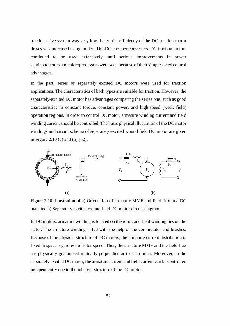
52

traction drive system was very low. Later, the efficiency of the DC traction motor

drives was increased using modern DC-DC chopper converters. DC traction motors

continued to be used extensively until serious improvements in power

semiconductors and microprocessors were seen because of their simple speed control

advantages.

In the past, series or separately excited DC motors were used for traction

applications. The characteristics of both types are suitable for traction. However, the

separately-excited DC motor has advantages comparing the series one, such as good

characteristics in constant torque, constant power, and high-speed (weak field)

operation regions. In order to control DC motor, armature winding current and field

winding current should be controlled. The basic physical illustration of the DC motor

windings and circuit schema of separately excited wound field DC motor are given

in Figure 2.10 (a) and (b) [62].

Ea

+++++++++

++++

+

-----

----

----

-

Lf

Commutator Brush

Ia

If

Armature

MMF (Ia)

Field Flux (If)

LaRa

Ia

-

+

Va Lf

Rf

-

+

Vf

If

(a) (b)

Figure 2.10. Illustration of a) Orientation of armature MMF and field flux in a DC

machine b) Separately excited wound field DC motor circuit diagram

In DC motors, armature winding is located on the rotor, and field winding lies on the

stator. The armature winding is fed with the help of the commutator and brushes.

Because of the physical structure of DC motors, the armature current distribution is

fixed in space regardless of rotor speed. Thus, the armature MMF and the field flux

are physically guaranteed mutually perpendicular to each other. Moreover, in the

separately excited DC motor, the armature current and field current can be controlled

independently due to the inherent structure of the DC motor.

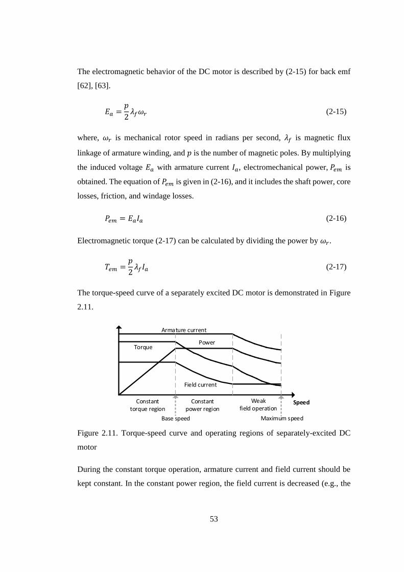
53

The electromagnetic behavior of the DC motor is described by (2-15) for back emf

[62], [63].

𝐸𝑎 =𝑝

2𝜆𝑓𝜔𝑟 (2-15)

where, 𝜔𝑟 is mechanical rotor speed in radians per second, 𝜆𝑓 is magnetic flux

linkage of armature winding, and 𝑝 is the number of magnetic poles. By multiplying

the induced voltage 𝐸𝑎 with armature current 𝐼𝑎, electromechanical power, 𝑃𝑒𝑚 is

obtained. The equation of 𝑃𝑒𝑚 is given in (2-16), and it includes the shaft power, core

losses, friction, and windage losses.

𝑃𝑒𝑚 = 𝐸𝑎𝐼𝑎 (2-16)

Electromagnetic torque (2-17) can be calculated by dividing the power by 𝜔𝑟.

𝑇𝑒𝑚 =𝑝

2𝜆𝑓𝐼𝑎 (2-17)

The torque-speed curve of a separately excited DC motor is demonstrated in Figure

2.11.

Weak field operation

Base speed Maximum speed

Constant power region

Armature current

PowerTorque

Field current

Constant torque region

Speed

Figure 2.11. Torque-speed curve and operating regions of separately-excited DC

motor

During the constant torque operation, armature current and field current should be

kept constant. In the constant power region, the field current is decreased (e.g., the

54

first region of field weakening operation) proportionally with the increased shaft

speed. In the last operating region (e.g., second field weakening region), the armature

current is reduced while the field flux is kept almost constant at a weak level. In this

region, the DC traction motor is operated at high speeds, and relatively high power

is supplied to train to keep operating speed almost constant [62].

2.2.2 Induction Motor

Two different types of three-phase induction motors are used for industrial

applications. These are called as squirrel cage and wound rotor induction motors.

The wound-rotor induction motors have also slip rings. For this reason, instead of

wound rotor induction motors, squirrel cage induction motors are preferred in

traction applications. In this study, squirrel cage induction motors will be referred to

as induction motors.

The induction motors have become more attractive with the development of

microprocessor-controlled power converters since 1980. They provide the following

advantages compared to DC motors [62].

- Quite high working speed & voltage because of no commutators and brushes,

- Higher robustness and reliability with a low maintenance requirement,

- High power density,

- Inherent regenerative braking capability,

- Steep torque-speed characteristics,

- Better electromagnetic compatibility due to the lack of brush-commutator

structure.

As mentioned in previous sections, three-phase induction motors are the most

mature technology among other traction motor options. The induction motor

consists of phase windings on the stator and conductor bars short-circuited with end

rings on the rotor. Induction motor stator windings are supplied with sinusoidal

55

balanced phase voltages at required magnitude and frequencies. The applied

voltages create currents in the stator windings, and as a result of the balanced phase

currents, a rotating magnetic field is obtained at the air gap. The rotating magnetic

field induces voltages and so currents on the rotor bars. The created rotor currents

interact with the rotating magnetic field, and as a result of this interaction, electro-

magnetic torque is created. Essentially, the induction motor resembles the

transformers, which have rotating secondary windings.

The basic physical representation of the three-phase induction motor is sketched in

Figure 2.12 [63].

xxxx

x

x

a+

a-

b-

c+

c-

b+

A+

A-

B-

C+

C-

B+

Stator

Rotor

Figure 2.12. A physical representation of a three-phase induction machine

The speed of an induction motor is mainly determined by its supply voltage and

frequency and shaft load. Figure 2.13 shows the per-phase induction motor

equivalent circuit in which rotor parameters are transferred to the stator side.

jwsLls jwsL lr

R r

1 - ss R

r

jwsLm Rc

Rs

Vph

+

-

Em

+

-

Figure 2.13. Per-phase equivalent circuit of induction machine

The input power 𝑃𝑝ℎ three components as given in (2-18)

𝑃𝑝ℎ = 𝑃𝑅𝑠 + 𝑃𝑎𝑔 + 𝑃𝑐 = 3𝑉𝑝ℎ𝐼𝑝ℎ cos Ø (2-18)

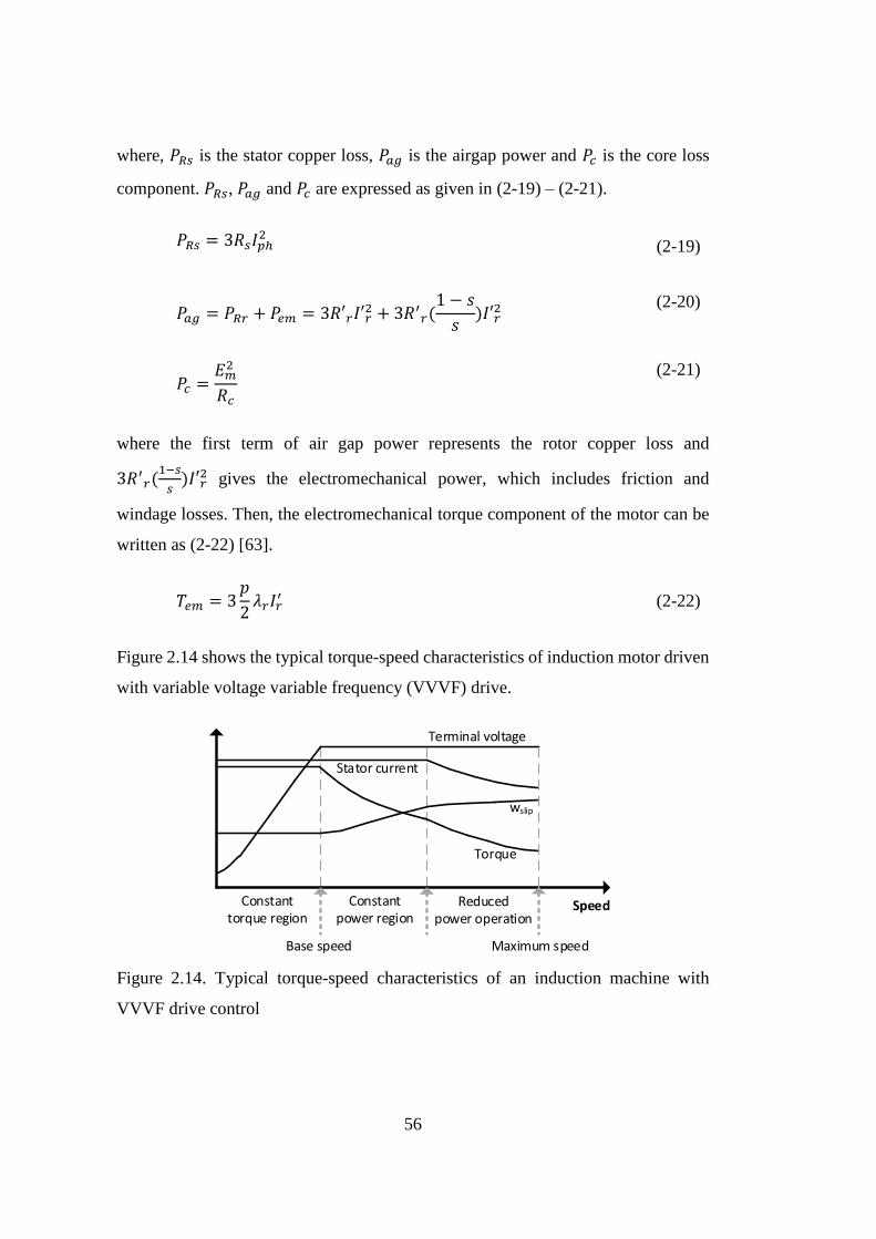
56

where, 𝑃𝑅𝑠 is the stator copper loss, 𝑃𝑎𝑔 is the airgap power and 𝑃𝑐 is the core loss

component. 𝑃𝑅𝑠, 𝑃𝑎𝑔 and 𝑃𝑐 are expressed as given in (2-19) – (2-21).

𝑃𝑅𝑠 = 3𝑅𝑠𝐼𝑝ℎ2 (2-19)

𝑃𝑎𝑔 = 𝑃𝑅𝑟 + 𝑃𝑒𝑚 = 3𝑅′𝑟𝐼′𝑟

2 + 3𝑅′𝑟(1 − 𝑠

𝑠)𝐼′𝑟

2 (2-20)

𝑃𝑐 =

𝐸𝑚2

𝑅𝑐

(2-21)

where the first term of air gap power represents the rotor copper loss and

3𝑅′𝑟(1−𝑠

𝑠)𝐼′𝑟

2 gives the electromechanical power, which includes friction and

windage losses. Then, the electromechanical torque component of the motor can be

written as (2-22) [63].

𝑇𝑒𝑚 = 3𝑝

2𝜆𝑟𝐼𝑟

′ (2-22)

Figure 2.14 shows the typical torque-speed characteristics of induction motor driven

with variable voltage variable frequency (VVVF) drive.

Stator current

Maximum speedBase speed

Terminal voltage

wslip

Torque

Reduced power operation

Constant power region

Constant torque region

Speed

Figure 2.14. Typical torque-speed characteristics of an induction machine with

VVVF drive control

57

The constant torque region, power region, and high-speed region (i.e., reduced power

region) can be implemented by varying the stator voltage and frequency. Control

methods of induction machines are introduced later in this chapter. In the constant

torque region, flux and torque components of current are kept as constant. In the

constant power region (field weakening region I), flux is decreased linearly with the

increased speed to keep T*Speed product constant. In field weakening region II at

high-speed operation, flux and torque components of current are further decreased

with the increasing speed by considering the electromagnetic design and thermal

limitations.

2.2.3 Permanent Magnet Synchronous Motor

The most distinct advantage of permanent magnet synchronous motor with respect

to the induction motor and DC motor is the absence of rotor windings. This leads to

improve efficiency and power density. The permanent magnets are placed on the

rotor instead of windings. NeFeB or SmCo alloys are commonly used to construct

rotor magnets. The inertia of the rotor is also reduced because of compact and small

size rotor structures. By considering the installation of the permanent magnet

materials, PMSMs are categorized into two groups, namely Surface Mounted

Permanent Magnet Synchronous Motors (SMPMSM) and Interior Permanent

Magnet Synchronous Motors (IPMSM). The rotor magnets are located on the rotor

surface for SMPMSMs, while magnets are buried in the rotor for IPMSMs. Basic

physical illustrations of PMSMs are given in Figure 2.15 (a) and (b) [63].

N

x

xx

S

a+

b+ c+

c-

a-

b-N

x

xx

S

a+

b+ c+

c-

a-

b-

Stator

Rotor

Magnet

(a) (b)

Figure 2.15. Basic physical representations of surface mounted and interior mounted

permanent magnet motors

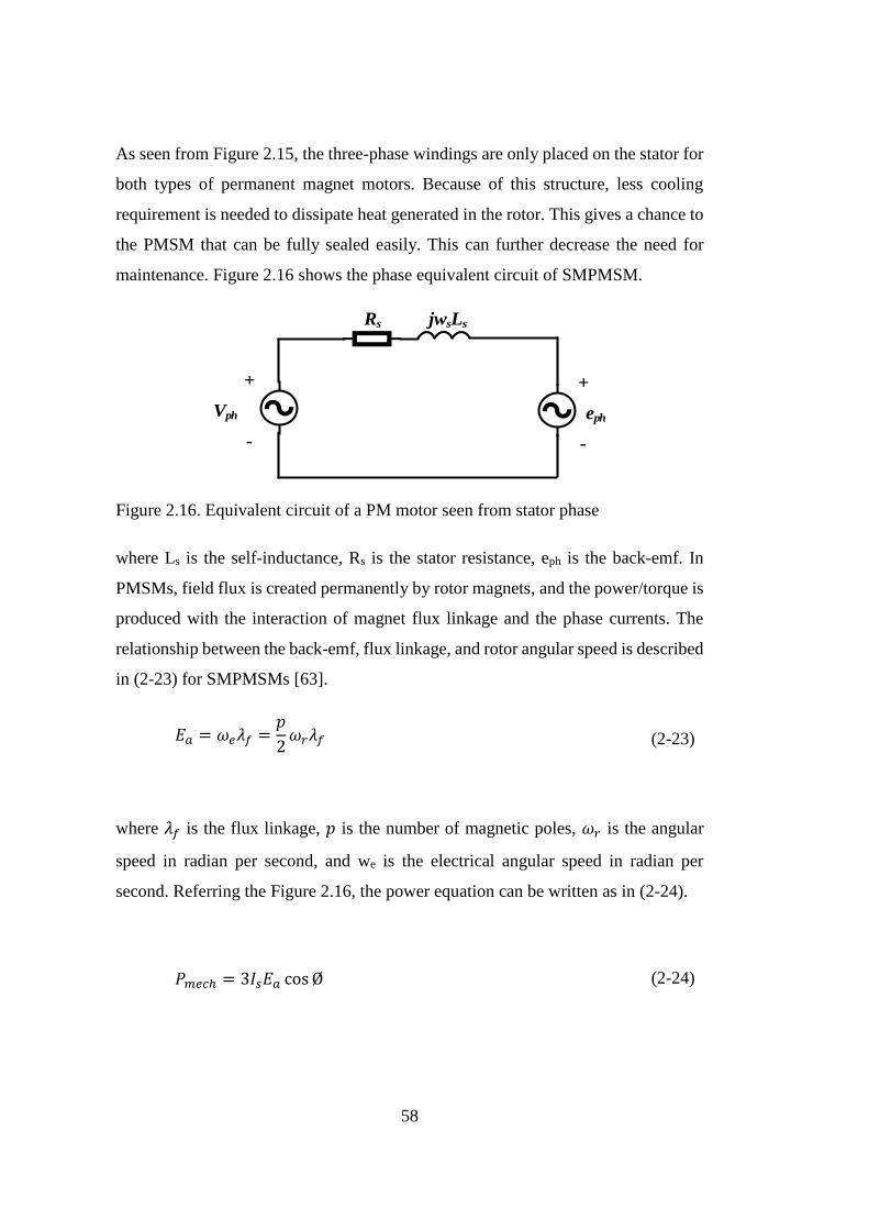
58

As seen from Figure 2.15, the three-phase windings are only placed on the stator for

both types of permanent magnet motors. Because of this structure, less cooling

requirement is needed to dissipate heat generated in the rotor. This gives a chance to

the PMSM that can be fully sealed easily. This can further decrease the need for

maintenance. Figure 2.16 shows the phase equivalent circuit of SMPMSM.

jwsLsRs

Vph

+

-

eph

+

-

Figure 2.16. Equivalent circuit of a PM motor seen from stator phase

where Ls is the self-inductance, Rs is the stator resistance, eph is the back-emf. In

PMSMs, field flux is created permanently by rotor magnets, and the power/torque is

produced with the interaction of magnet flux linkage and the phase currents. The

relationship between the back-emf, flux linkage, and rotor angular speed is described

in (2-23) for SMPMSMs [63].

𝐸𝑎 = 𝜔𝑒𝜆𝑓 =𝑝

2𝜔𝑟𝜆𝑓 (2-23)

where 𝜆𝑓 is the flux linkage, 𝑝 is the number of magnetic poles, 𝜔𝑟 is the angular

speed in radian per second, and we is the electrical angular speed in radian per

second. Referring the Figure 2.16, the power equation can be written as in (2-24).

𝑃𝑚𝑒𝑐ℎ = 3𝐼𝑠𝐸𝑎 cos Ø (2-24)

59

By substituting (2-23) in (2-24) and then, by dividing the power equation by wr, the

output torque of SMPMSMs can be computed as in (2-25).

𝑇𝑚𝑒𝑐ℎ = 3𝑝

2𝐼𝑠𝜆𝑓 cos Ø (2-25)

Unlike SMPMSMs, additional torque can be obtained for IPMSMs because of the

reluctance torque. In addition to this, IPMSMs have good overload capability and

good efficiency values at high speeds compared to SMPMSMs. Moreover, IPMSMs

have a more robust structure, and demagnetization of their magnets is difficult since

the magnets are physically buried in the rotor. These make IPMSMs more suitable

for high-speed applications. However, the price of IPMSMs is particularly higher

than SMPMSMs [64].

2.2.4 Comparison of Traction Motors

Technological advances in power electronics have made different motor types more

advantageous over time. From past to now on, DC motors, induction motors, and

PMSMs have been used in traction applications. As mentioned in several sections,

performance, cost, reliability, efficiency, maintenance, weight, size, and

electromagnetic compatibility form the main considerations for traction applications.

Because of easy control features, adequate performance and torque-speed

characteristics, low price, and easy constructions, DC motors were used to some

extent in the past. Later, rugged structure, high efficiency, low cost, and less

maintenance features make induction motors more attractive with the advance of

semiconductors and microprocessors. Nowadays, PMSMs are seen as one of the

convenient motor types for traction applications. However, issues such as high price,

production complexity, magnet needs, and safety-critical issues limit the spread of

PMSMs. A comparative evaluation of major traction motor types is summarized in

Table 2.2.

60

Table 2.2 The Comparison of Different Types of Traction Motors

Motor Type

Attribute SMPMSM IPMSM IM DC Motor

Efficiency +++ +++ ++ +

Size +++ +++ ++ +

Cost ++ ++ +++ +++

Rotor Cooling +++ +++ + +

High-Speed Operation ++ +++ +++ +

Service and Maintenance +++ +++ +++ +

Fault Tolerance + ++ +++ +

Overload Capacity ++ +++ +++ ++

Parallel Operation + + +++ +++

Prevalence of New Railway

Applications + + +++ +

DC motors are not preferred anymore due to speed and voltage limitations, low

efficiency, and high maintenance requirements. Among the other motor types,

induction motors have superior fault tolerance capability, prevalence, and cost

advantage. The efficiency is slightly lower, but it is still very close to PMSMs. The

excitation can be easily removed for induction machines at any speed. This is

preferred for rail vehicles manufacturers for safety reasons. However, in PMSMs,

excitation cannot be removed due to the permanent magnets; induced voltage will

create current. This current will continue to circulate in the winding as long as the

motor is in motion. Therefore, it is not simply sufficient to turn-off the

semiconductors because of the antiparallel diodes. It should be considered in the

motor and drive system design. However, this makes the motor heavier, less

efficient, and more expensive. On the other hand, a few precautions may be taken

into account in the traction converter design, such as the use of circuit breakers or

contactors between motor and inverter. Despite all these precautions, this problem

may not be solved and may require additional actions if a permanent short circuit

occurs at the motor side. In order to solve this, the gearbox may be decoupled at the

failure instant. These also increase the cost of the drive system. This especially

requires high price coupling between traction motor and gearbox. Moreover, the

permanent magnet flux also creates an additional disadvantage in the coasting mode;

61

even the semiconductors and main input contactors are switched off, induced emf is

generated. It will end up with an increase in DC-link voltage and may damage

semiconductors and capacitors or decrease the lifetime of semiconductors and

capacitors at high speed. In order to get rid of this problem, voltage ratings of

components can be selected according to this high voltage level. However, this will

end up with increased size, increased cost, and decreased efficiency. Moreover, in

order to exit coasting mode and re-accelerate the vehicle, special control algorithms

should be taken into account. DC-link voltage can be equalized by applying field

weakening with a very small amount of negative torque. This is necessary to keep

the DC-link voltage as stable while producing de-magnetizing current. As soon as

the DC-link voltage is equal to the DC input voltage, the main line contactors can be

closed. These solutions increase the control system complexity and the cost of the

system [63]. On the other hand, PMSMs have higher power densities and efficiencies

compared to DC motors and induction motors. Because of these features,

SMPMSMs and IPMSMs are adopted for a few traction applications. Due to their

low weight and size, PMSMs may provide certain advantages for low-floor tramway

vehicles which have very limited space on their bogies.

Induction motors and IPMSMs have good overload capacities, while SMPMSMs

have limitations for overload. Additionally, high-speed operation is more suitable

for induction motors and IPMSMs due to the mechanical structures. Surface-

mounted magnets create disadvantages for the high-speed operation of SMPMSM.

In addition to this, induction machines are suitable for parallel driving, which is often

preferred in rail transportation. All evaluations show that asynchronous motors are

the most advantageous in existing system solutions [65].

2.3 Topological Overview of Two-Level Voltage Source Traction Inverters

The function of a voltage source inverter is to convert a DC voltage to an AC voltage

waveform with variable magnitude and frequency. In Figure 2.17, the circuit diagram

of a two-level voltage source inverter is given. Fully controllable six semiconductor

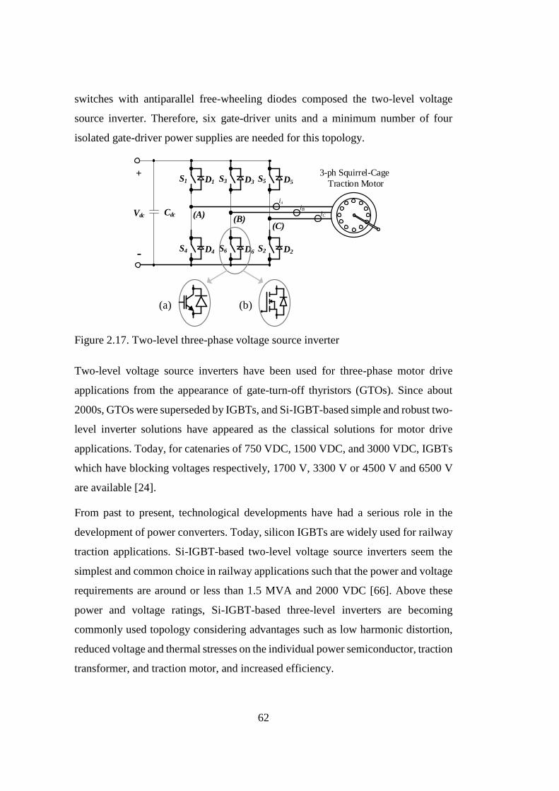
62

switches with antiparallel free-wheeling diodes composed the two-level voltage

source inverter. Therefore, six gate-driver units and a minimum number of four

isolated gate-driver power supplies are needed for this topology.

(A)(B)

(C)

iA

+

-

3-ph Squirrel-Cage

Traction MotorS1

Cdc

D1

Vdc

S3 D3 S5 D5

S4 D4 S6 D6 S2 D2

iB

iC

(a) (b)

Figure 2.17. Two-level three-phase voltage source inverter

Two-level voltage source inverters have been used for three-phase motor drive

applications from the appearance of gate-turn-off thyristors (GTOs). Since about

2000s, GTOs were superseded by IGBTs, and Si-IGBT-based simple and robust two-

level inverter solutions have appeared as the classical solutions for motor drive

applications. Today, for catenaries of 750 VDC, 1500 VDC, and 3000 VDC, IGBTs

which have blocking voltages respectively, 1700 V, 3300 V or 4500 V and 6500 V

are available [24].

From past to present, technological developments have had a serious role in the

development of power converters. Today, silicon IGBTs are widely used for railway

traction applications. Si-IGBT-based two-level voltage source inverters seem the

simplest and common choice in railway applications such that the power and voltage

requirements are around or less than 1.5 MVA and 2000 VDC [66]. Above these

power and voltage ratings, Si-IGBT-based three-level inverters are becoming

commonly used topology considering advantages such as low harmonic distortion,

reduced voltage and thermal stresses on the individual power semiconductor, traction

transformer, and traction motor, and increased efficiency.

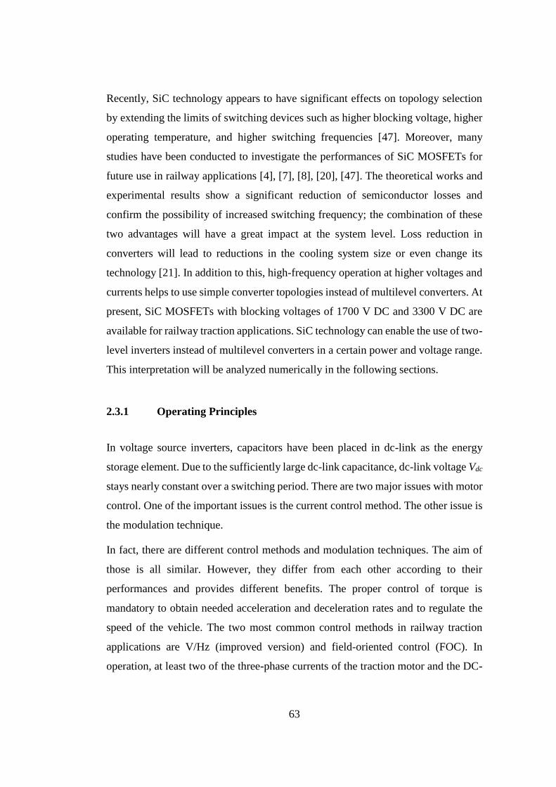
63

Recently, SiC technology appears to have significant effects on topology selection

by extending the limits of switching devices such as higher blocking voltage, higher

operating temperature, and higher switching frequencies [47]. Moreover, many

studies have been conducted to investigate the performances of SiC MOSFETs for

future use in railway applications [4], [7], [8], [20], [47]. The theoretical works and

experimental results show a significant reduction of semiconductor losses and

confirm the possibility of increased switching frequency; the combination of these

two advantages will have a great impact at the system level. Loss reduction in

converters will lead to reductions in the cooling system size or even change its

technology [21]. In addition to this, high-frequency operation at higher voltages and

currents helps to use simple converter topologies instead of multilevel converters. At

present, SiC MOSFETs with blocking voltages of 1700 V DC and 3300 V DC are

available for railway traction applications. SiC technology can enable the use of two-

level inverters instead of multilevel converters in a certain power and voltage range.

This interpretation will be analyzed numerically in the following sections.

2.3.1 Operating Principles

In voltage source inverters, capacitors have been placed in dc-link as the energy

storage element. Due to the sufficiently large dc-link capacitance, dc-link voltage Vdc

stays nearly constant over a switching period. There are two major issues with motor

control. One of the important issues is the current control method. The other issue is

the modulation technique.

In fact, there are different control methods and modulation techniques. The aim of

those is all similar. However, they differ from each other according to their

performances and provides different benefits. The proper control of torque is

mandatory to obtain needed acceleration and deceleration rates and to regulate the

speed of the vehicle. The two most common control methods in railway traction

applications are V/Hz (improved version) and field-oriented control (FOC). In

operation, at least two of the three-phase currents of the traction motor and the DC-

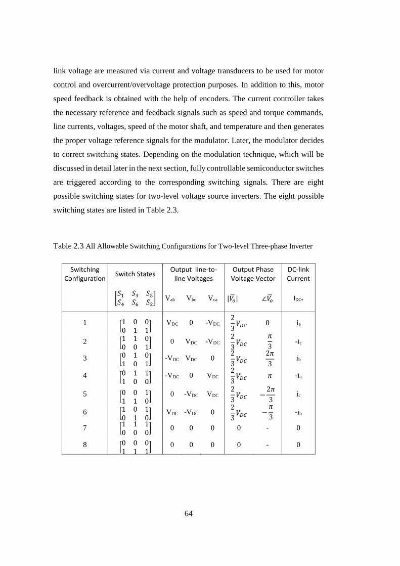
64

link voltage are measured via current and voltage transducers to be used for motor

control and overcurrent/overvoltage protection purposes. In addition to this, motor

speed feedback is obtained with the help of encoders. The current controller takes

the necessary reference and feedback signals such as speed and torque commands,

line currents, voltages, speed of the motor shaft, and temperature and then generates

the proper voltage reference signals for the modulator. Later, the modulator decides

to correct switching states. Depending on the modulation technique, which will be

discussed in detail later in the next section, fully controllable semiconductor switches

are triggered according to the corresponding switching signals. There are eight

possible switching states for two-level voltage source inverters. The eight possible

switching states are listed in Table 2.3.

Table 2.3 All Allowable Switching Configurations for Two-level Three-phase Inverter

Switching Configuration

Switch States Output line-to-

line Voltages Output Phase

Voltage Vector DC-link Current

[𝑆1 𝑆3 𝑆5𝑆4 𝑆6 𝑆2

] Vab Vbc Vca |𝑉�̅�| ∠𝑉�̅� IDC+

1 [1 0 00 1 1

] VDC 0 -VDC 2

3𝑉𝐷𝐶 0 ia

2 [1 1 00 0 1

] 0 VDC -VDC 2

3𝑉𝐷𝐶

𝜋

3 -ic

3 [0 1 01 0 1

] -VDC VDC 0 2

3𝑉𝐷𝐶

2𝜋

3 ib

4 [0 1 11 0 0

] -VDC 0 VDC 2

3𝑉𝐷𝐶 𝜋 -ia

5 [0 0 11 1 0

] 0 -VDC VDC 2

3𝑉𝐷𝐶 −

2𝜋

3 ic

6 [1 0 10 1 0

] VDC -VDC 0 2

3𝑉𝐷𝐶 −

𝜋

3 -ib

7 [1 1 10 0 0

] 0 0 0 0 - 0

8 [0 0 01 1 1

] 0 0 0 0 - 0

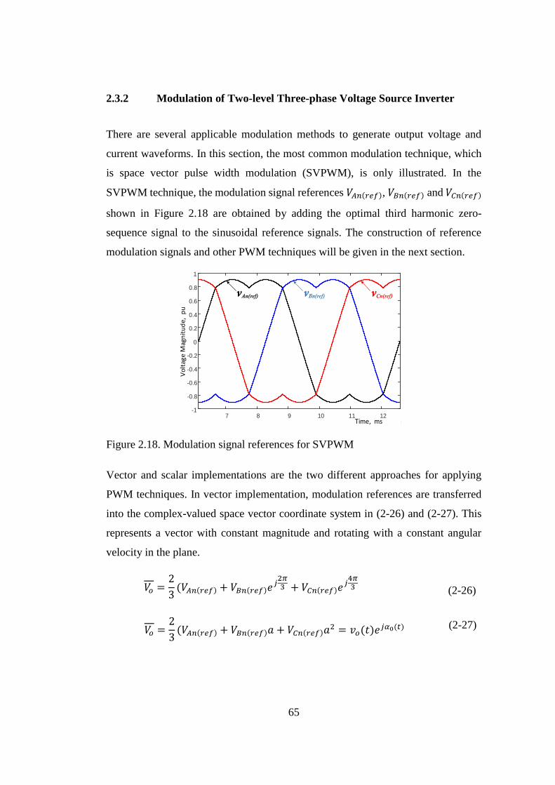
65

2.3.2 Modulation of Two-level Three-phase Voltage Source Inverter

There are several applicable modulation methods to generate output voltage and

current waveforms. In this section, the most common modulation technique, which

is space vector pulse width modulation (SVPWM), is only illustrated. In the

SVPWM technique, the modulation signal references 𝑉𝐴𝑛(𝑟𝑒𝑓), 𝑉𝐵𝑛(𝑟𝑒𝑓) and 𝑉𝐶𝑛(𝑟𝑒𝑓)

shown in Figure 2.18 are obtained by adding the optimal third harmonic zero-

sequence signal to the sinusoidal reference signals. The construction of reference

modulation signals and other PWM techniques will be given in the next section.

7 8 9 10 11 12

10-3

-1

-0.8

-0.6

-0.4

-0.2

0

0.2

0.4

0.6

0.8

1

vAn(ref) vCn(ref)vBn(ref)

Time, ms

Vo

ltag

e M

agn

itu

de

, p

u

Figure 2.18. Modulation signal references for SVPWM

Vector and scalar implementations are the two different approaches for applying

PWM techniques. In vector implementation, modulation references are transferred

into the complex-valued space vector coordinate system in (2-26) and (2-27). This

represents a vector with constant magnitude and rotating with a constant angular

velocity in the plane.

𝑉𝑜 =

2

3(𝑉𝐴𝑛(𝑟𝑒𝑓) + 𝑉𝐵𝑛(𝑟𝑒𝑓)𝑒

𝑗2𝜋3 + 𝑉𝐶𝑛(𝑟𝑒𝑓)𝑒

𝑗4𝜋3 (2-26)

𝑉𝑜 =2

3(𝑉𝐴𝑛(𝑟𝑒𝑓) + 𝑉𝐵𝑛(𝑟𝑒𝑓)𝑎 + 𝑉𝐶𝑛(𝑟𝑒𝑓)𝑎

2 = 𝑣𝑜(𝑡)𝑒𝑗𝛼0(𝑡) (2-27)

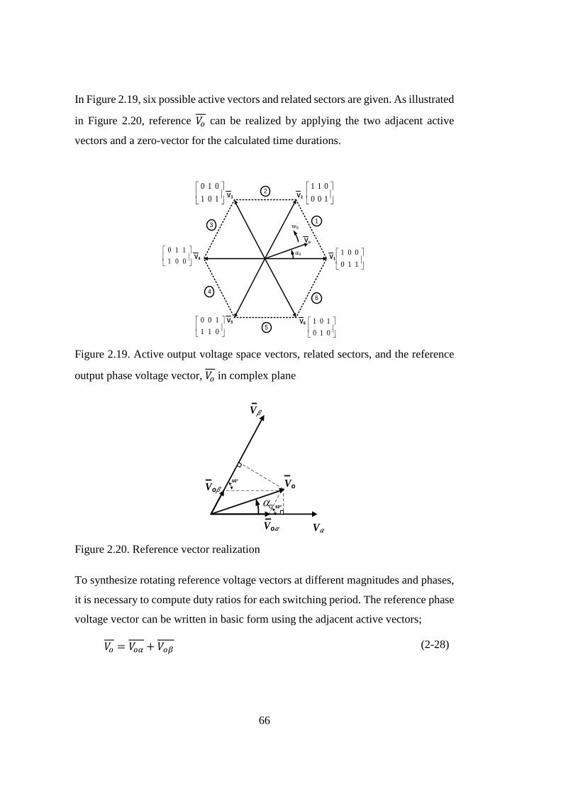
66

In Figure 2.19, six possible active vectors and related sectors are given. As illustrated

in Figure 2.20, reference 𝑉𝑜 can be realized by applying the two adjacent active

vectors and a zero-vector for the calculated time durations.

V1

1

2

3

4

5

6

Vo

𝛼0

w0

V2V3

V4

V5 V6

1

0

1

0

0

1

1

0

0

1

0

1

1

0

0

1

1

0

0

1

0

1

1

0

0

1

1

0

1

0

0

1

1

0

0

1

Figure 2.19. Active output voltage space vectors, related sectors, and the reference

output phase voltage vector, 𝑉𝑜 in complex plane

VoVo

Vo𝛼 V𝛼

V

o 60°

60°

Figure 2.20. Reference vector realization

To synthesize rotating reference voltage vectors at different magnitudes and phases,

it is necessary to compute duty ratios for each switching period. The reference phase

voltage vector can be written in basic form using the adjacent active vectors;

𝑉𝑜 = 𝑉𝑜𝛼 + 𝑉𝑜𝛽 (2-28)

67

with

𝑉𝑜𝛼 = 𝑉𝛼 𝛿𝛼

𝑉𝑜𝛽 = 𝑉𝛽 𝛿𝛽

(2-29)

Then, the duty ratios are;

𝛿𝛼 =|𝑉𝑜𝛼|

|𝑉𝛼|

𝛿𝛽 =|𝑉𝑜𝛽|

|𝑉𝛽|

(2-30)

Also, |𝑉𝑜𝛼| =|𝑉𝑜| 𝑠𝑖𝑛(

𝜋

3−𝛼0)

𝑠𝑖𝑛(𝜋

3)

, |𝑉𝑜𝛽| =|𝑉𝑜| 𝑠𝑖𝑛(𝛼0)

𝑠𝑖𝑛(𝜋

3)

.

Hence, the duty ratios can be written as;

𝛿𝛼 =

|𝑉𝑜|

√3

2|𝑉𝛼|

𝑠𝑖𝑛 (𝜋

3− 𝛼0), 𝛿𝛽 =

|𝑉𝑜|

√3

2|𝑉𝛽|

𝑠𝑖𝑛 (𝛼0)

(2-31)

|𝑉𝛼| = |𝑉𝛽| =2

3|𝑉𝐷𝐶|,

√3|𝑉𝑜|

|𝑉𝐷𝐶|= 𝑚𝑖 𝑎𝑛𝑑 0 ≤ 𝑚𝑖 ≤ 1

where 𝑚𝑖 is the voltage modulation index, which represents the input to output

voltage transfer ratio, and VDC is the average value of the DC-link voltage. Thus, the

duty ratios of the active vectors can be written as;

𝛿𝛼 = 𝑚𝑖 sin (𝜋

3− 𝛼0) =

𝑇𝛼𝑇𝑠

𝛿𝛽 = 𝑚𝑖 sin(𝛼0) =𝑇𝛽

𝑇𝑠

(2-32)

After calculating the duty ratios 𝑑𝛼 and 𝑑𝛽, the duty ratio of the zero-phase voltage vector

can be written as follow;

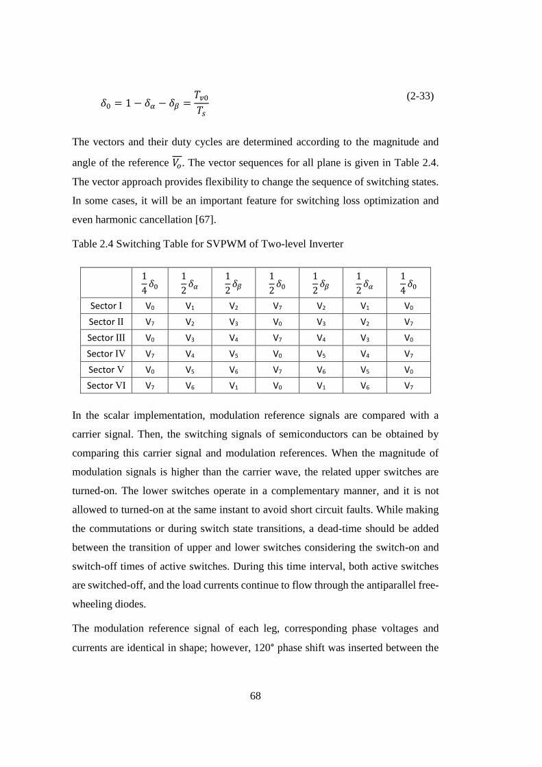
68

𝛿0 = 1 − 𝛿𝛼 − 𝛿𝛽 =

𝑇𝑣0𝑇𝑠

(2-33)

The vectors and their duty cycles are determined according to the magnitude and

angle of the reference 𝑉𝑜. The vector sequences for all plane is given in Table 2.4.

The vector approach provides flexibility to change the sequence of switching states.

In some cases, it will be an important feature for switching loss optimization and

even harmonic cancellation [67].

Table 2.4 Switching Table for SVPWM of Two-level Inverter

1

4𝛿0

1

2𝛿𝛼

1

2𝛿𝛽

1

2𝛿0

1

2𝛿𝛽

1

2𝛿𝛼

1

4𝛿0

Sector Ⅰ V0 V1 V2 V7 V2 V1 V0

Sector Ⅱ V7 V2 V3 V0 V3 V2 V7

Sector Ⅲ V0 V3 V4 V7 V4 V3 V0

Sector Ⅳ V7 V4 V5 V0 V5 V4 V7

Sector Ⅴ V0 V5 V6 V7 V6 V5 V0

Sector Ⅵ V7 V6 V1 V0 V1 V6 V7

In the scalar implementation, modulation reference signals are compared with a

carrier signal. Then, the switching signals of semiconductors can be obtained by

comparing this carrier signal and modulation references. When the magnitude of

modulation signals is higher than the carrier wave, the related upper switches are

turned-on. The lower switches operate in a complementary manner, and it is not

allowed to turned-on at the same instant to avoid short circuit faults. While making

the commutations or during switch state transitions, a dead-time should be added

between the transition of upper and lower switches considering the switch-on and

switch-off times of active switches. During this time interval, both active switches

are switched-off, and the load currents continue to flow through the antiparallel free-

wheeling diodes.

The modulation reference signal of each leg, corresponding phase voltages and

currents are identical in shape; however, 120° phase shift was inserted between the

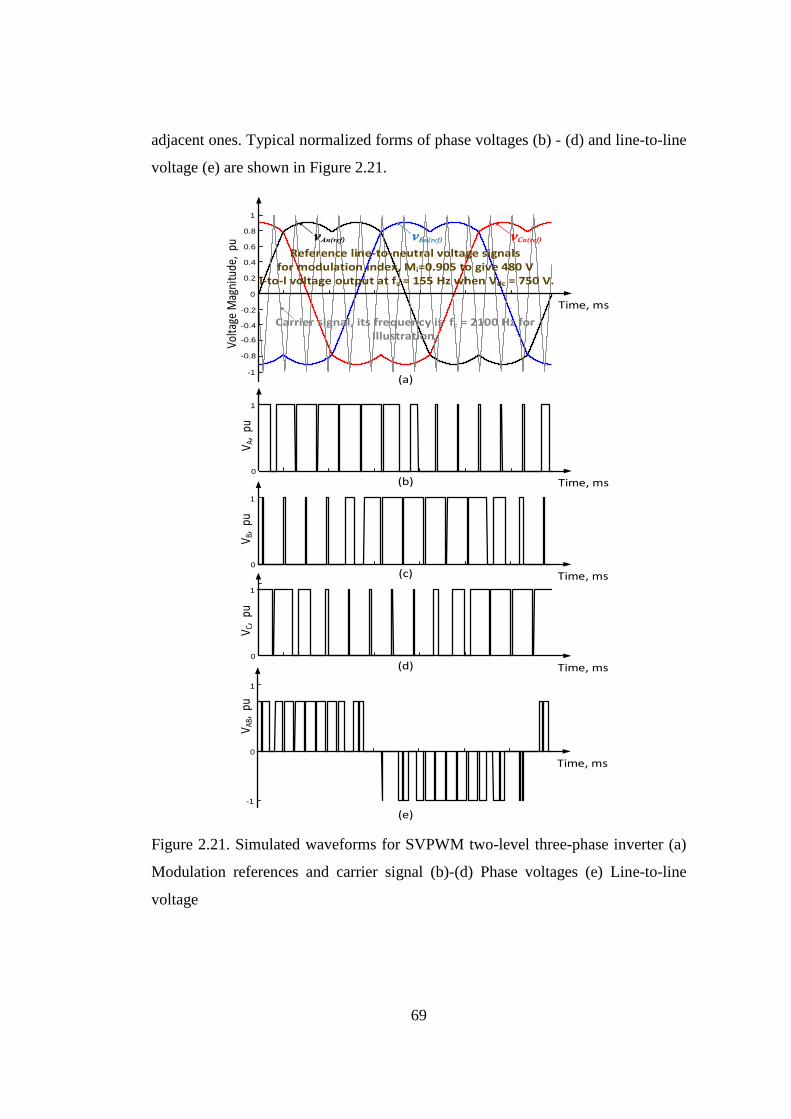
69

adjacent ones. Typical normalized forms of phase voltages (b) - (d) and line-to-line

voltage (e) are shown in Figure 2.21.

-1

-0.8

-0.6

-0.4

-0.2

0

0.2

0.4

0.6

0.8

1

vAn(ref) vCn(ref)vBn(ref)

Reference line-to-neutral voltage signalsfor modulation index, Mi=0.905 to give 480 V

l-to-l voltage output at fs = 155 Hz when Vdc = 750 V.

Carrier signal, its frequency is fc = 2100 Hz for illustration.

Time, ms

Volta

ge M

agni

tude

, pu

0

Time, ms

1

V A,

pu

0

Time, ms

1

V B,

pu

0

Time, ms

1

V C,

pu

0

Time, ms

1

V AB,

pu

-1

(a)

(b)

(c)

(d)

(e)


Modulation references and carrier signal (b)-(d) Phase voltages (e) Line-to-line

voltage

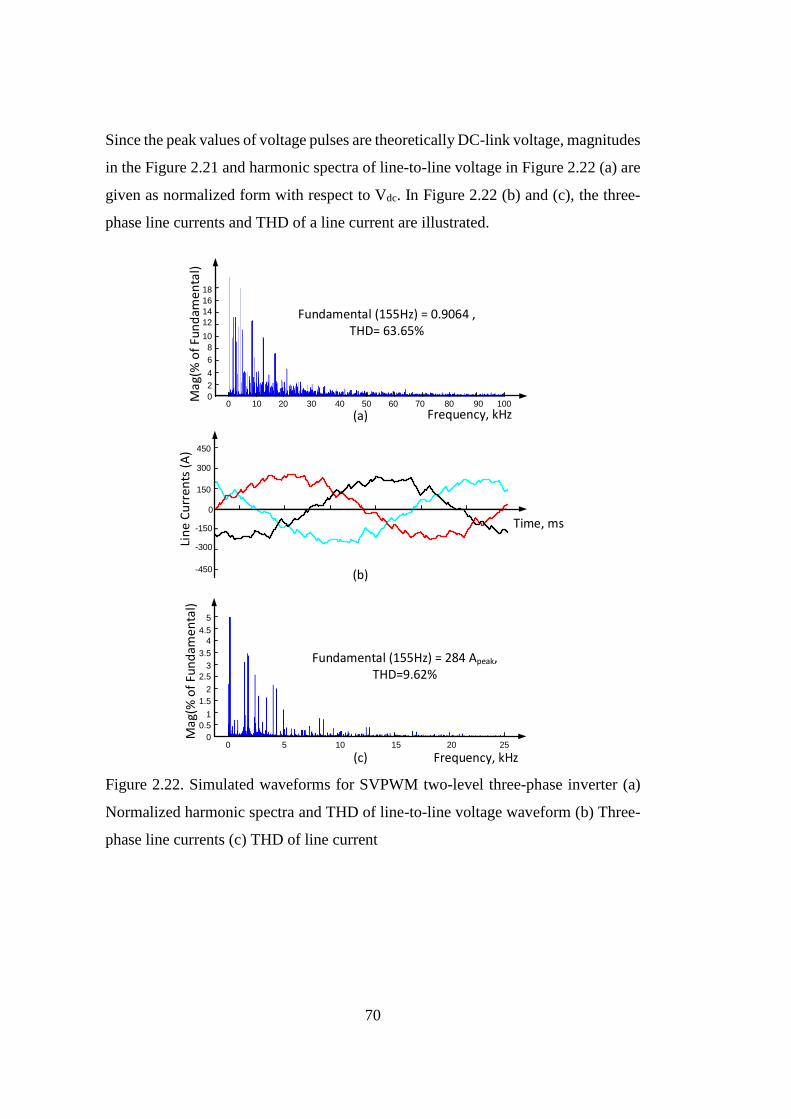
70

Since the peak values of voltage pulses are theoretically DC-link voltage, magnitudes

in the Figure 2.21 and harmonic spectra of line-to-line voltage in Figure 2.22 (a) are

given as normalized form with respect to Vdc. In Figure 2.22 (b) and (c), the three-

phase line currents and THD of a line current are illustrated.

Fundamental (155Hz) = 0.9064 , THD= 63.65%

Ma

g(%

of

Fun

dam

en

tal)

Frequency, kHz0 10

0

18

16

14

12

10

8

6

4

2

20 30 40 50 60 70 80 90 100

0

Time, ms

300

Lin

e C

urr

en

ts (

A)

-450

150

-150

-300

450

0

Frequency, kHz

Ma

g(%

of

Fun

dam

en

tal)

0 5 10 15 20 25

5

4.5

4

3.5

3

2.5

2

1.5

1

0.5

Fundamental (155Hz) = 284 Apeak, THD=9.62%

(a)

(b)

(c)


Normalized harmonic spectra and THD of line-to-line voltage waveform (b) Three-

phase line currents (c) THD of line current

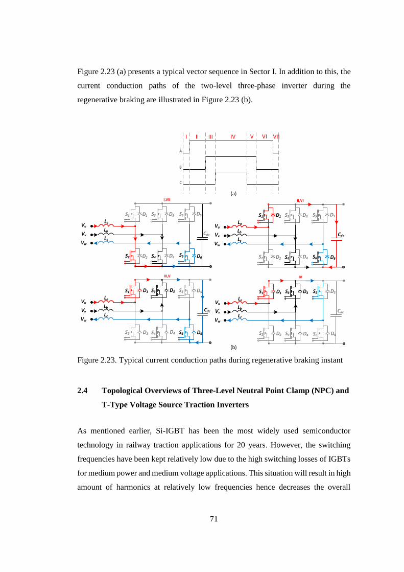
71

Figure 2.23 (a) presents a typical vector sequence in Sector I. In addition to this, the

current conduction paths of the two-level three-phase inverter during the

regenerative braking are illustrated in Figure 2.23 (b).

S1

S2

S3

S4S6

Cdc

S5

Lb

La

Lc

Vu

Vv

Vw

I,VII

S1

S2

S3

S4 S6

Cdc

S5

Lb

La

Lc

Vu

Vv

Vw

II,VI

III,V IV

S1

S2

S3

S4 S6

Cdc

S5

Lb

La

Lc

Vu

Vv

Vw

S1

S2

S3

S4 S6

Cdc

S5

Lb

La

Lc

Vu

Vv

Vw

D1

D2

D3

D4

D5

D6

D1

D2

D3

D4

D5

D6

D1

D2

D3

D4

D5

D6

D1

D2

D3

D4

D5

D6

(a)

(b)

A

B

C

I II III IV V VI VII

Figure 2.23. Typical current conduction paths during regenerative braking instant

2.4 Topological Overviews of Three-Level Neutral Point Clamp (NPC) and

T-Type Voltage Source Traction Inverters

As mentioned earlier, Si-IGBT has been the most widely used semiconductor

technology in railway traction applications for 20 years. However, the switching

frequencies have been kept relatively low due to the high switching losses of IGBTs

for medium power and medium voltage applications. This situation will result in high

amount of harmonics at relatively low frequencies hence decreases the overall

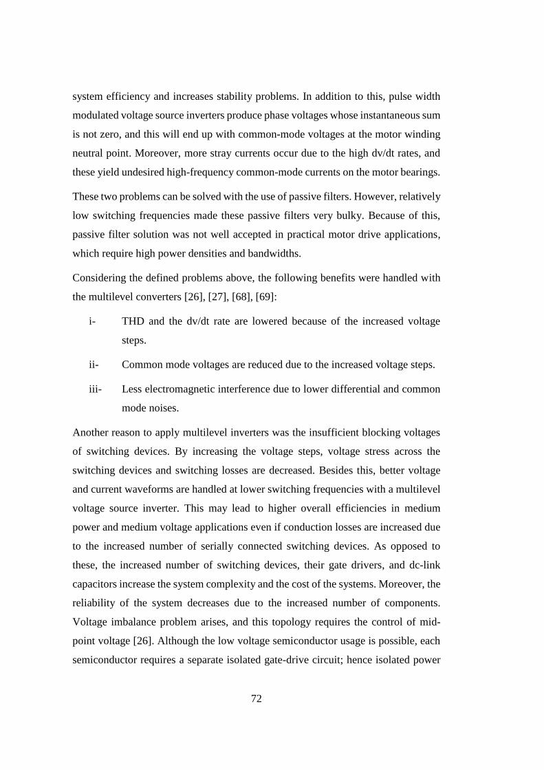
72

system efficiency and increases stability problems. In addition to this, pulse width

modulated voltage source inverters produce phase voltages whose instantaneous sum

is not zero, and this will end up with common-mode voltages at the motor winding

neutral point. Moreover, more stray currents occur due to the high dv/dt rates, and

these yield undesired high-frequency common-mode currents on the motor bearings.

These two problems can be solved with the use of passive filters. However, relatively

low switching frequencies made these passive filters very bulky. Because of this,

passive filter solution was not well accepted in practical motor drive applications,

which require high power densities and bandwidths.

Considering the defined problems above, the following benefits were handled with

the multilevel converters [26], [27], [68], [69]:

i- THD and the dv/dt rate are lowered because of the increased voltage

steps.

ii- Common mode voltages are reduced due to the increased voltage steps.

iii- Less electromagnetic interference due to lower differential and common

mode noises.

Another reason to apply multilevel inverters was the insufficient blocking voltages

of switching devices. By increasing the voltage steps, voltage stress across the

switching devices and switching losses are decreased. Besides this, better voltage

and current waveforms are handled at lower switching frequencies with a multilevel

voltage source inverter. This may lead to higher overall efficiencies in medium

power and medium voltage applications even if conduction losses are increased due

to the increased number of serially connected switching devices. As opposed to

these, the increased number of switching devices, their gate drivers, and dc-link

capacitors increase the system complexity and the cost of the systems. Moreover, the

reliability of the system decreases due to the increased number of components.

Voltage imbalance problem arises, and this topology requires the control of mid-

point voltage [26]. Although the low voltage semiconductor usage is possible, each

semiconductor requires a separate isolated gate-drive circuit; hence isolated power

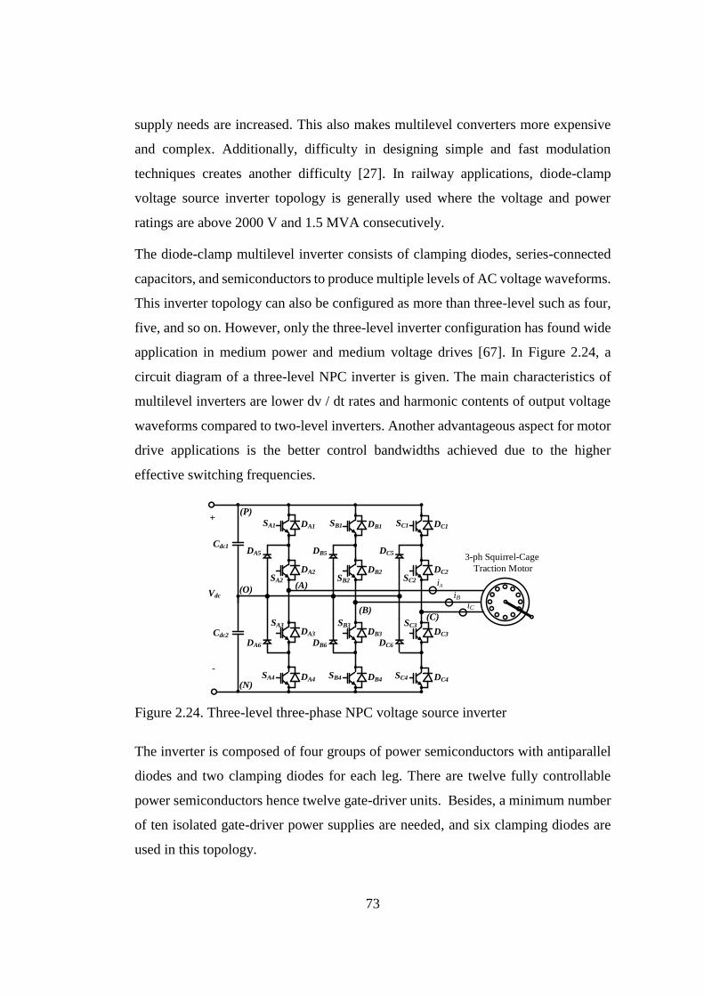
73

supply needs are increased. This also makes multilevel converters more expensive

and complex. Additionally, difficulty in designing simple and fast modulation

techniques creates another difficulty [27]. In railway applications, diode-clamp

voltage source inverter topology is generally used where the voltage and power

ratings are above 2000 V and 1.5 MVA consecutively.

The diode-clamp multilevel inverter consists of clamping diodes, series-connected

capacitors, and semiconductors to produce multiple levels of AC voltage waveforms.

This inverter topology can also be configured as more than three-level such as four,

five, and so on. However, only the three-level inverter configuration has found wide

application in medium power and medium voltage drives [67]. In Figure 2.24, a

circuit diagram of a three-level NPC inverter is given. The main characteristics of

multilevel inverters are lower dv / dt rates and harmonic contents of output voltage

waveforms compared to two-level inverters. Another advantageous aspect for motor

drive applications is the better control bandwidths achieved due to the higher

effective switching frequencies.

3-ph Squirrel-Cage

Traction Motor

+

-

Vdc

Cdc2

Cdc1DA5

DA6

DB5

DB6

DC5

DC6

iA

iB

iC

SA2

DA2

SA1 DA1

SA4 DA4

SA3

DA3

SB2

DB2

SB1 DB1

SB4 DB4

SB3

DB3

SC2

DC2

SC1 DC1

SC4 DC4

SC3

DC3

(P)

(N)

(O)(A)

(B)(C)

Figure 2.24. Three-level three-phase NPC voltage source inverter

The inverter is composed of four groups of power semiconductors with antiparallel

diodes and two clamping diodes for each leg. There are twelve fully controllable

power semiconductors hence twelve gate-driver units. Besides, a minimum number

of ten isolated gate-driver power supplies are needed, and six clamping diodes are

used in this topology.

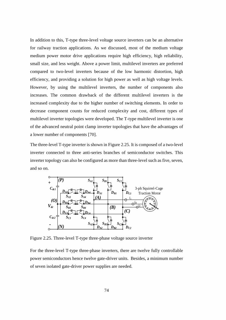
74

In addition to this, T-type three-level voltage source inverters can be an alternative

for railway traction applications. As we discussed, most of the medium voltage

medium power motor drive applications require high efficiency, high reliability,

small size, and less weight. Above a power limit, multilevel inverters are preferred

compared to two-level inverters because of the low harmonic distortion, high

efficiency, and providing a solution for high power as well as high voltage levels.

However, by using the multilevel inverters, the number of components also

increases. The common drawback of the different multilevel inverters is the

increased complexity due to the higher number of switching elements. In order to

decrease component counts for reduced complexity and cost, different types of

multilevel inverter topologies were developed. The T-type multilevel inverter is one

of the advanced neutral point clamp inverter topologies that have the advantages of

a lower number of components [70].

The three-level T-type inverter is shown in Figure 2.25. It is composed of a two-level

inverter connected to three anti-series branches of semiconductor switches. This

inverter topology can also be configured as more than three-level such as five, seven,

and so on.

(C)(B)

(A)

(N)

(O)

(P)

Vdc

Cdc1

SA2DA2

iA

3-ph Squirrel-Cage

Traction Motor

+

-

Cdc2

DC1

SC1

SC2

DC2

iB

iC

DB1

SB1

SB2

DB2

DA1

SA1

SA3

DA3

SA4

DA4

SB3

DB3

SB4

DB4

SC3

DC3

SC4

DC4

Figure 2.25. Three-level T-type three-phase voltage source inverter

For the three-level T-type three-phase inverters, there are twelve fully controllable

power semiconductors hence twelve gate-driver units. Besides, a minimum number

of seven isolated gate-driver power supplies are needed.

75

2.4.1 Operating Principles of Three-level NPC and T-Type Voltage Source

Traction Inverters

The DC-link capacitor is split into two series-connected capacitors for a three-level

NPC inverter. The voltage of each capacitor is equal to Vdc/2. When the SA1 and SA2

are turned-on, the output terminal (A) is connected to the most positive rail of the

DC bus, which is denoted as (P). When SA2 and SA3 are turned-on, the terminal of (A)

is connected to the mid-point of DC-link (O), which has a voltage value of Vdc/2. If

SA3 and SA4 are turned-on, the terminal of (A) is connected to the negative bus, which

is denoted as (N). Similarly, the same switching states create the same results for

other legs. By considering the voltage levels of all three phases, the inverter has a

total of twenty-seven possible switching states, as listed in Table 2.5. The voltage

waveforms of VAO, VBO, and VCO have three levels, +Vdc/2, 0, and -Vdc/2.

Similarly, the DC-link capacitor is split into two series-connected capacitors for a

three-level T-type inverter. The voltage of each capacitor is equal to Vdc/2. In order

to achieve the three different voltage levels with respect to the midpoint, high side

semiconductor switch, low side semiconductor switch, or semiconductor switches of

anti-series branches are controlled. The voltage levels +Vdc/2, -Vdc/2, and 0 are

obtained, respectively. In fact, the turned-on and turned-off switches of NPC and T-

type inverters are different; however, the voltage vectors are the same. Considering

the operation of all phases, a common list for switching states of NPC and T-type

three-level three-phase can be given in Table 2.5. P-type vectors represent the small

voltage vectors that are obtained using the upper half of the DC-link capacitors, while

the N-type small vectors use the lower half of the DC-link.

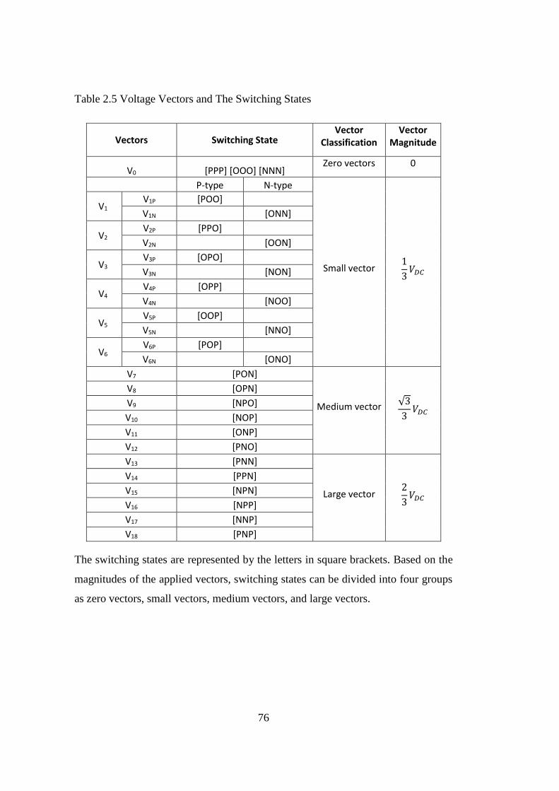
76

Table 2.5 Voltage Vectors and The Switching States

Vectors Switching State Vector

Classification Vector

Magnitude

V0 [PPP] [OOO] [NNN] Zero vectors 0

P-type N-type

Small vector 1

3𝑉𝐷𝐶

V1 V1P [POO]

V1N [ONN]

V2 V2P [PPO]

V2N [OON]

V3 V3P [OPO]

V3N [NON]

V4 V4P [OPP]

V4N [NOO]

V5 V5P [OOP]

V5N [NNO]

V6 V6P [POP]

V6N [ONO]

V7 [PON]

Medium vector √3

3𝑉𝐷𝐶

V8 [OPN]

V9 [NPO]

V10 [NOP]

V11 [ONP]

V12 [PNO]

V13 [PNN]

Large vector 2

3𝑉𝐷𝐶

V14 [PPN]

V15 [NPN]

V16 [NPP]

V17 [NNP]

V18 [PNP]

The switching states are represented by the letters in square brackets. Based on the

magnitudes of the applied vectors, switching states can be divided into four groups

as zero vectors, small vectors, medium vectors, and large vectors.

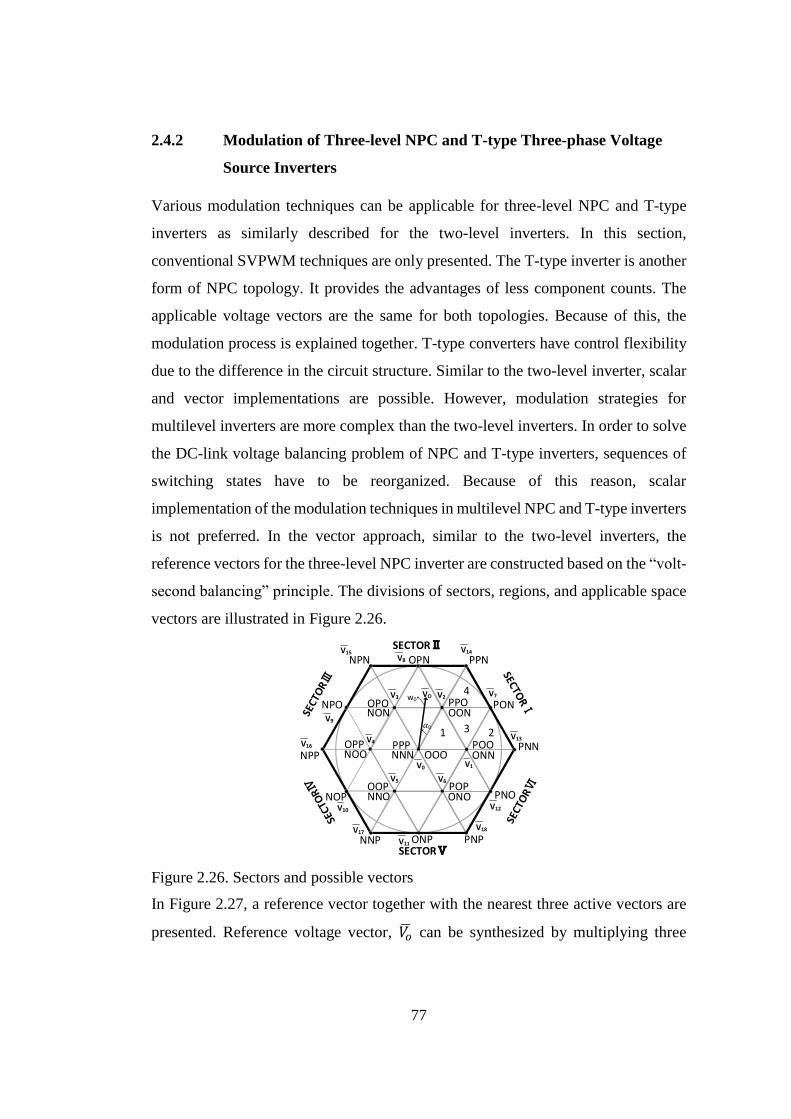
77

2.4.2 Modulation of Three-level NPC and T-type Three-phase Voltage

Source Inverters

Various modulation techniques can be applicable for three-level NPC and T-type

inverters as similarly described for the two-level inverters. In this section,

conventional SVPWM techniques are only presented. The T-type inverter is another

form of NPC topology. It provides the advantages of less component counts. The

applicable voltage vectors are the same for both topologies. Because of this, the

modulation process is explained together. T-type converters have control flexibility

due to the difference in the circuit structure. Similar to the two-level inverter, scalar

and vector implementations are possible. However, modulation strategies for

multilevel inverters are more complex than the two-level inverters. In order to solve

the DC-link voltage balancing problem of NPC and T-type inverters, sequences of

switching states have to be reorganized. Because of this reason, scalar

implementation of the modulation techniques in multilevel NPC and T-type inverters

is not preferred. In the vector approach, similar to the two-level inverters, the

reference vectors for the three-level NPC inverter are constructed based on the “volt-

second balancing” principle. The divisions of sectors, regions, and applicable space

vectors are illustrated in Figure 2.26.

OOONNNPPP

OONPPO

PPN

PON

PNN

PNO

PNPONPNNP

NOP

NPPPOOONN

POPONO

OOPNNO

OPPNOO

OPONON

OPNNPN

NPO

1 3 2

4

SECTORⅡ

SECTORⅤ

V1

V2V3

V4

V5 V6

V0

V7

V8

V9

V10

V11

V12

V13

V14V15

V16

V17V18

VO

0

w0

Figure 2.26. Sectors and possible vectors

In Figure 2.27, a reference vector together with the nearest three active vectors are

presented. Reference voltage vector, 𝑉�̅� can be synthesized by multiplying three

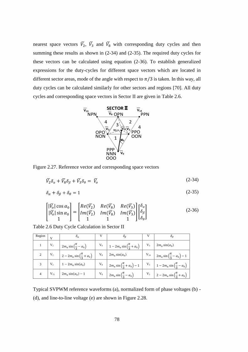
78

nearest space vectors 𝑉2̅, 𝑉3̅ and 𝑉8̅ with corresponding duty cycles and then

summing these results as shown in (2-34) and (2-35). The required duty cycles for

these vectors can be calculated using equation (2-36). To establish generalized

expressions for the duty-cycles for different space vectors which are located in

different sector areas, mode of the angle with respect to 𝜋/3 is taken. In this way, all

duty cycles can be calculated similarly for other sectors and regions [70]. All duty

cycles and corresponding space vectors in Sector II are given in Table 2.6.

OOONNNPPP

OONPPO

PPN

OPONON

OPNNPN

1

4

SECTORⅡ

V2V3

V0

V8

V14V15

VO

0

w0

324

Figure 2.27. Reference vector and corresponding space vectors

𝑉2̅𝛿𝛼 + 𝑉8̅𝛿 + 𝑉3̅𝛿𝜃 = 𝑉�̅� (2-34)

𝛿𝛼 + 𝛿𝛽 + 𝛿𝜃 = 1 (2-35)

[|𝑉�̅�| cos 𝛼0|𝑉�̅�| sin 𝛼0

1

] = [𝑅𝑒(𝑉2̅) 𝑅𝑒(𝑉8̅) 𝑅𝑒(𝑉3̅)

𝐼𝑚(𝑉2̅) 𝐼𝑚(𝑉8̅) 𝐼𝑚(𝑉3̅)1 1 1

] [

𝛿𝛼𝛿 𝛿𝜃

] (2-36)

Table 2.6 Duty Cycle Calculation in Sector II

Region V

𝛿𝛼 V 𝛿𝛽 V 𝛿𝜃

1 V2 2𝑚𝑎 sin (𝜋

3− 𝛼0) V0 1 − 2𝑚𝑎 sin (

𝜋

3+ 𝛼0) V3 2𝑚𝑎 sin(𝛼0)

2 V2 2 − 2𝑚𝑎 sin (𝜋

3+ 𝛼0) V8 2𝑚𝑎 sin(𝛼0) V14 2𝑚𝑎 sin (

𝜋

3− 𝛼0) − 1

3 V2 1 − 2𝑚𝑎 sin(𝛼0) V8 2𝑚𝑎 sin (𝜋

3+ 𝛼0) − 1 V3 1 − 2𝑚𝑎 sin (

𝜋

3− 𝛼0)

4 V15 2𝑚𝑎 sin(𝛼0) − 1 V8 2𝑚𝑎 sin (𝜋

3− 𝛼0) V3 2 − 2𝑚𝑎 sin (

𝜋

3+ 𝛼0)

Typical SVPWM reference waveforms (a), normalized form of phase voltages (b) -

(d), and line-to-line voltage (e) are shown in Figure 2.28.

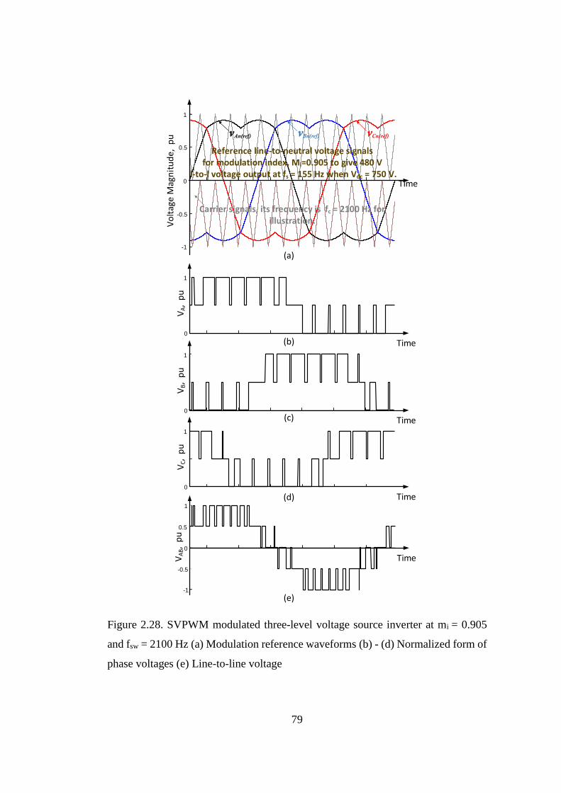
79


l-to-l voltage output at fs = 155 Hz when Vdc = 750 V.

Carrier signals, its frequency is fc = 2100 Hz for illustration.

-1

-0.5

0

0.5

1

Time

Vo

ltag

e M

agn

itu

de

, p

u vAn(ref) vCn(ref)vBn(ref)

0

Time

1

VA,

pu

0

Time

1

VB,

pu

0

Time

1

VC,

pu

0

Time

1

VA

B,

pu

-1

-0.5

0.5

(a)

(b)

(c)

(d)

(e)


and fsw = 2100 Hz (a) Modulation reference waveforms (b) - (d) Normalized form of

phase voltages (e) Line-to-line voltage

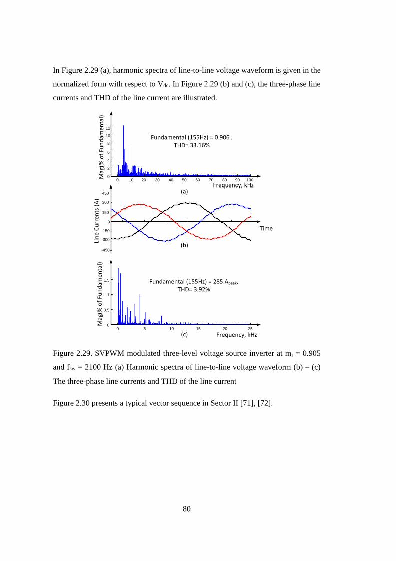
80

In Figure 2.29 (a), harmonic spectra of line-to-line voltage waveform is given in the

normalized form with respect to Vdc. In Figure 2.29 (b) and (c), the three-phase line

currents and THD of the line current are illustrated.


Mag

(% o

f Fu

nd

amen

tal)

Frequency, kHz0 10

0

12

10

8

6

4

2

20 30 40 50 60 70 80 90 100

0

Time

300

Lin

e C

urr

ents

(A

)

-450

150

-150

-300

450

0

Frequency, kHz

Mag

(% o

f Fu

nd

amen

tal)

0 5 10 15 20 25

1.5

1

0.5

Fundamental (155Hz) = 285 Apeak, THD= 3.92%

(a)

(b)

(c)


and fsw = 2100 Hz (a) Harmonic spectra of line-to-line voltage waveform (b) – (c)

The three-phase line currents and THD of the line current

Figure 2.30 presents a typical vector sequence in Sector II [71], [72].

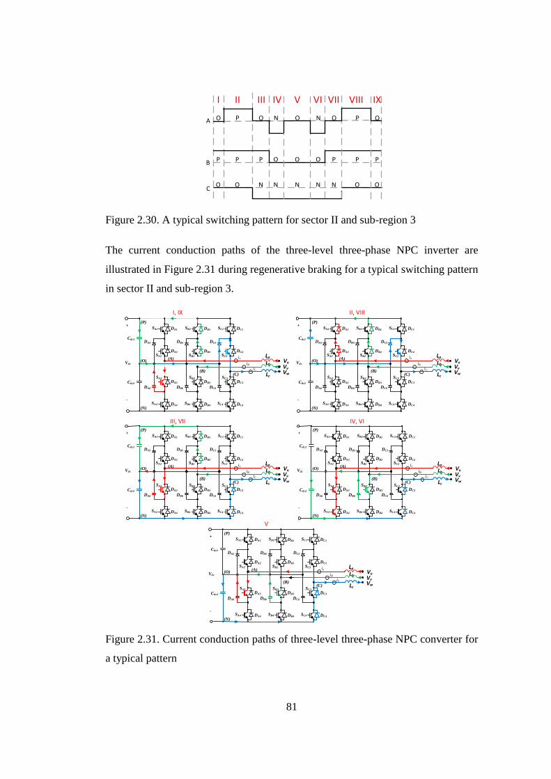
81

A

B

C

I II III IV VI VIIV VIII IX

O P O N O N O P O

P P P O O O P P P

O O N N N N N O O

Figure 2.30. A typical switching pattern for sector II and sub-region 3

The current conduction paths of the three-level three-phase NPC inverter are

illustrated in Figure 2.31 during regenerative braking for a typical switching pattern

in sector II and sub-region 3.

+

-

Vdc

Cdc2

Cdc1DA5

DA6

DB5

DB6

DC5

DC6

iA

iB

iC

SA2

DA2

SA1 DA1

SA4 DA4

SA3

DA3

SB2

DB2

SB1 DB1

SB4 DB4

SB3

DB3

SC2

DC2

SC1 DC1

SC4 DC4

SC3

DC3

(P)

(N)

(O)(A)

(B)(C)

Lb

La

Lc

Vu

VvVw

I, IX

+

-

Vdc

Cdc2

Cdc1DA5

DA6

DB5

DB6

DC5

DC6

iA

iB

iC

SA2

DA2

SA1 DA1

SA4 DA4

SA3

DA3

SB2

DB2

SB1 DB1

SB4 DB4

SB3

DB3

SC2

DC2

SC1 DC1

SC4 DC4

SC3

DC3

(P)

(N)

(O)(A)

(B)(C)

Lb

La

Lc

Vu

VvVw

+

-

Vdc

Cdc2

Cdc1DA5

DA6

DB5

DB6

DC5

DC6

iA

iB

iC

SA2

DA2

SA1 DA1

SA4 DA4

SA3

DA3

SB2

DB2

SB1 DB1

SB4 DB4

SB3

DB3

SC2

DC2

SC1 DC1

SC4 DC4

SC3

DC3

(P)

(N)

(O)(A)

(B)(C)

Lb

La

Lc

Vu

VvVw

+

-

Vdc

Cdc2

Cdc1DA5

DA6

DB5

DB6

DC5

DC6

iA

iB

iC

SA2

DA2

SA1 DA1

SA4 DA4

SA3

DA3

SB2

DB2

SB1 DB1

SB4 DB4

SB3

DB3

SC2

DC2

SC1 DC1

SC4 DC4

SC3

DC3

(P)

(N)

(O)(A)

(B)(C)

Lb

La

Lc

Vu

VvVw

+

-

Vdc

Cdc2

Cdc1DA5

DA6

DB5

DB6

DC5

DC6

iA

iB

iC

SA2

DA2

SA1 DA1

SA4 DA4

SA3

DA3

SB2

DB2

SB1 DB1

SB4 DB4

SB3

DB3

SC2

DC2

SC1 DC1

SC4 DC4

SC3

DC3

(P)

(N)

(O)(A)

(B)(C)

Lb

La

Lc

Vu

VvVw

II, VIII

III, VII IV, VI

V

Figure 2.31. Current conduction paths of three-level three-phase NPC converter for

a typical pattern

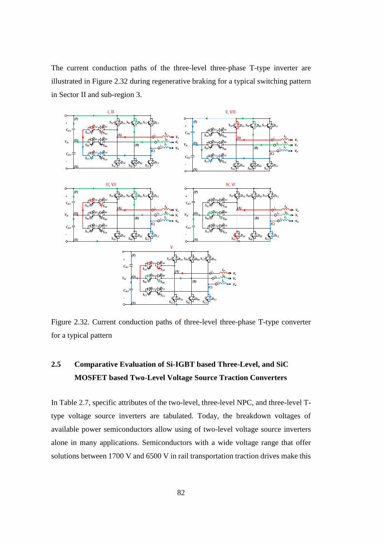
82

The current conduction paths of the three-level three-phase T-type inverter are

illustrated in Figure 2.32 during regenerative braking for a typical switching pattern

in Sector II and sub-region 3.

+

-

Vdc

Cdc2

Cdc1

SA2

DA2

SA1 DA1

SB2

DB2

SB1 DB1

SC2

DC2

SC1 DC1

(P)

(N)

(O)

(A)Lb

La

Lc

Vu

Vv

Vw

SA4

DA4

SA3

DA3

SB4

DB4

SB3

DB3

SC4

DC4

SC3

DC3

iA

iB

iC(B)

(C)

+

-

Vdc

Cdc2

Cdc1

SA2

DA2

SA1 DA1

SB2

DB2

SB1 DB1

SC2

DC2

SC1 DC1

(P)

(N)

(O)

(A)Lb

La

Lc

Vu

Vv

Vw

SA4

DA4

SA3

DA3

SB4

DB4

SB3

DB3

SC4

DC4

SC3

DC3

iA

iB

iC(B)

(C)

+

-

Vdc

Cdc2

Cdc1

SA2

DA2

SA1 DA1

SB2

DB2

SB1 DB1

SC2

DC2

SC1 DC1

(P)

(N)

(O)

(A)Lb

La

Lc

Vu

Vv

Vw

SA4

DA4

SA3

DA3

SB4

DB4

SB3

DB3

SC4

DC4

SC3

DC3

iA

iB

iC(B)

(C)

+

-

Vdc

Cdc2

Cdc1

SA2

DA2

SA1 DA1

SB2

DB2

SB1 DB1

SC2

DC2

SC1 DC1

(P)

(N)

(O)

(A)Lb

La

Lc

Vu

Vv

Vw

SA4

DA4

SA3

DA3

SB4

DB4

SB3

DB3

SC4

DC4

SC3

DC3

iA

iB

iC(B)

(C)

+

-

Vdc

Cdc2

Cdc1

SA2

DA2

SA1 DA1

SB2

DB2

SB1 DB1

SC2

DC2

SC1 DC1

(P)

(N)

(O)

(A)Lb

La

Lc

Vu

Vv

Vw

SA4

DA4

SA3

DA3

SB4

DB4

SB3

DB3

SC4

DC4

SC3

DC3

iA

iB

iC(B)

(C)

I, IX II, VIII

III, VII IV, VI

V

Figure 2.32. Current conduction paths of three-level three-phase T-type converter

for a typical pattern

2.5 Comparative Evaluation of Si-IGBT based Three-Level, and SiC

MOSFET based Two-Level Voltage Source Traction Converters

In Table 2.7, specific attributes of the two-level, three-level NPC, and three-level T-

type voltage source inverters are tabulated. Today, the breakdown voltages of

available power semiconductors allow using of two-level voltage source inverters

alone in many applications. Semiconductors with a wide voltage range that offer

solutions between 1700 V and 6500 V in rail transportation traction drives make this

83

situation similar. As can be seen from the table below, if we do not take into account

the stresses due to power loss, the two-level solution seems to offer a significant

advantage in terms of MTBF. However, this is not the case in reality. The switching

losses have greatly limited the switching frequency of the two-level topology and

severely reduced the power quality. In fact, in order to solve this restriction and

continue with the choice of two-level inverter topology, special modulation

techniques such as Selective Harmonic Elimination Pulse Width Modulation

(SHEPWM), Selective Harmonic Mitigation Pulse Width Modulation (SHMPWM),

and Optimal Pulse Width Modulation (OPWM) are used to decrease switching

losses. They will be explained in more detail in the next section. This solution may

require lots of offline computations to find the optimum angles of the pulses for

different modulation index. If anyone wants to do all those by online calculations,

more powerful graphical processing units are needed. In addition, this solution also

requires modification in the motor control methods (e.g., switching from vector

control to scalar control methods). Because of this, multilevel converters have to be

used in medium voltage and medium power railway traction applications.

From now on, the reduced switching losses together with higher blocking voltage

capability make it possible to use simpler SiC-based two-level voltage source

inverters instead of multilevel inverters. In order words, by using SiC MOSFETs,

the switching frequency can be increased by a considerable amount because of the

inherently reduced switching losses. Thus, harmonic distortions on the voltage and

current waveforms can be seriously reduced without the need for multilevel

converters for a certain power and voltage level. In addition, the conduction losses

are also decreased a considerable amount because of the number of serially used

semiconductor devices in multilevel converters. Besides these, the reliability of the

converter is also increased as a result of the decrease in the number of serially

connected semiconductor devices and the higher operating temperature. In fact, these

improvements will not enable two-level inverters to be used in all power and voltage

ranges. However, it will greatly expand the power and voltage levels, causing the

topology changes between two-level to three-level inverters. The exact border of this

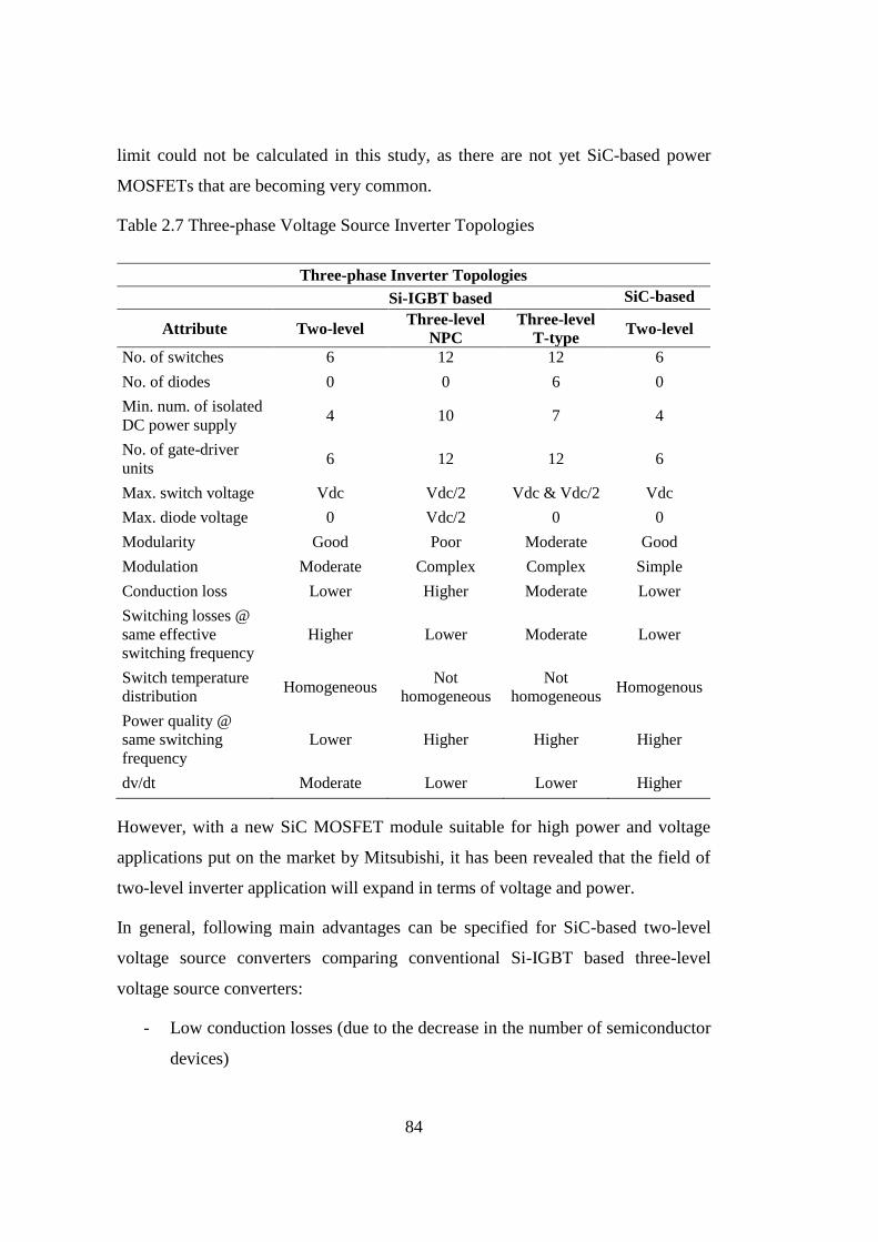
84

limit could not be calculated in this study, as there are not yet SiC-based power

MOSFETs that are becoming very common.

Table 2.7 Three-phase Voltage Source Inverter Topologies

Three-phase Inverter Topologies

Si-IGBT based SiC-based

Attribute Two-level Three-level

NPC

Three-level

T-type Two-level

No. of switches 6 12 12 6

No. of diodes 0 0 6 0

Min. num. of isolated

DC power supply 4 10 7 4

No. of gate-driver

units 6 12 12 6

Max. switch voltage Vdc Vdc/2 Vdc & Vdc/2 Vdc

Max. diode voltage 0 Vdc/2 0 0

Modularity Good Poor Moderate Good

Modulation Moderate Complex Complex Simple

Conduction loss Lower Higher Moderate Lower

Switching losses @

same effective

switching frequency

Higher Lower Moderate Lower

Switch temperature

distribution Homogeneous

Not

homogeneous

Not

homogeneous Homogenous

Power quality @

same switching

frequency

Lower Higher Higher Higher

dv/dt Moderate Lower Lower Higher

However, with a new SiC MOSFET module suitable for high power and voltage

applications put on the market by Mitsubishi, it has been revealed that the field of

two-level inverter application will expand in terms of voltage and power.

In general, following main advantages can be specified for SiC-based two-level

voltage source converters comparing conventional Si-IGBT based three-level

voltage source converters:

- Low conduction losses (due to the decrease in the number of semiconductor

devices)

85

- Low switching losses (e.g., an inherent feature of SiC devices, higher

switching frequencies, and smaller reactive components)

- Higher operating temperatures (e.g., less cooling requirements)

- Higher blocking voltages

- Higher power densities

- Low complexity

- High reliability

However, as opposed to these, the stresses on insulation materials, especially the

motor winding insulations, are increased due to the high dv/dt rates. This situation

may increase the stray currents flowing through the winding insulation materials to

the chassis and may shorten the life of insulation materials. Moreover, this also

increases the bearing currents and shaft voltage. In general, bearing currents and

shaft voltage can cause accelerated degradation of the motor. Therefore, stronger

insulation material (e.g., Kapton, isolated bearings, ground brushes for rotor shaft)

should be preferred for such applications.

2.6 Voltage and Current Waveform Synthesizing

The developments in fully controllable power switches and high-speed digital

processors have made various modulation methods applicable for power converters.

In principle, the aims of the modulation methods are to synthesize the desired voltage

and current waveforms from the input source [67]. Nowadays, IGBT-based

induction motor drives are the most common solution for railway applications.

However, due to high switching losses as in high power and medium voltage drives,

IGBT switching frequencies are limited between 500 Hz-3 kHz. This situation

reduces voltage and current waveform quality, especially at medium power and

relatively high speeds drives. The distortions on waveforms may be brought to

sufficient levels by using combinations of special modulation methods. However, it

increases the workload of the algorithm and requires pre-computational effort, and

86

also increases the complexity. In addition to this, strong computational ability such

as GPU is needed if all operations are required to be done online.

2.6.1 Pulse Width Modulation Methods

In the past, six-step modulation was commonly used for motor drive applications at

constant power and high-speed regions due to the allowable low switching frequency

limits. However, this method creates low order harmonics (such as 5th, 7th, 11th, so

on) with considerable magnitudes. Development in the semiconductor area reduces

the switching losses significantly, and this loss reduction gives a chance to operate

higher switching frequencies. As a result of this, utilization of various PWM methods

has been possible for various applications. Thus, elimination or reduction of

significant low order harmonics became possible depending on the power

requirements.

Today, many pulse width modulation methods are widely used for synthesizing

output voltage and current waveforms of inverters. The frequency and the magnitude

of the inverter output voltage and current waveforms can be controlled with low

harmonic content. The harmonic content of the output waveforms is strictly related

to the applied number of pulses. In fact, the better harmonic content is achieved with

the increased switching frequency. However, the increased switching losses still

create a strong limit to increase switching frequency. Therefore, there is a trade-off

between the reduction of the harmonics and the switching losses. In addition to this,

not only the switching frequency but also applied PWM methods also have a strong

influence on inverter/motor losses, harmonics as well as additional noise and

vibration [73]. The most common PWM techniques used for motor drive applications

are Sinusoidal Pulse Width Modulation (SPWM), SVPWM, Third Harmonic

Injection Pulse Width Modulation (THIPWM), Discontinuous Pulse Width

Modulation (DPWM), and programmed Pulse Width Modulation [74]. Moreover,

SHEPWM, SHMPWM, and OPWM techniques are also used in railway traction

applications [58].

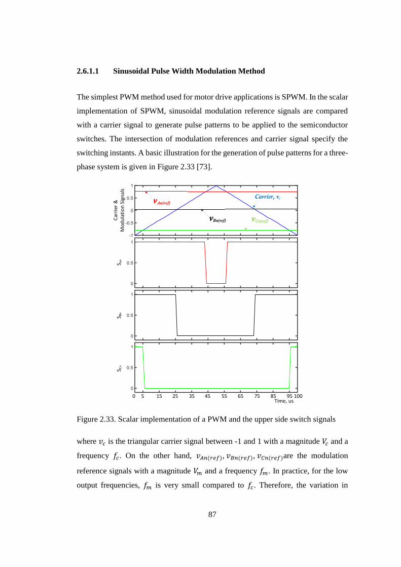
87

2.6.1.1 Sinusoidal Pulse Width Modulation Method

The simplest PWM method used for motor drive applications is SPWM. In the scalar

implementation of SPWM, sinusoidal modulation reference signals are compared

with a carrier signal to generate pulse patterns to be applied to the semiconductor

switches. The intersection of modulation references and carrier signal specify the

switching instants. A basic illustration for the generation of pulse patterns for a three-

phase system is given in Figure 2.33 [73].

5Time, us

15 25 35 45 55 65 75 85 95 1000

vAn(ref)

vCn(ref)vBn(ref)Car

rier

&

Mod

ulat

ion

Sign

als

S a+

S B+

S C+

Carrier, vc

Figure 2.33. Scalar implementation of a PWM and the upper side switch signals

where 𝑣𝑐 is the triangular carrier signal between -1 and 1 with a magnitude 𝑉𝑐 and a

frequency 𝑓𝑐. On the other hand, 𝑣𝐴𝑛(𝑟𝑒𝑓), 𝑣𝐵𝑛(𝑟𝑒𝑓), 𝑣𝐶𝑛(𝑟𝑒𝑓)are the modulation

reference signals with a magnitude 𝑉𝑚 and a frequency 𝑓𝑚. In practice, for the low

output frequencies, 𝑓𝑚 is very small compared to 𝑓𝑐. Therefore, the variation in

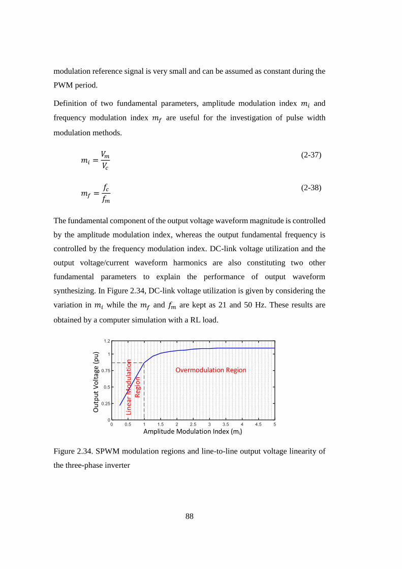
88

modulation reference signal is very small and can be assumed as constant during the

PWM period.

Definition of two fundamental parameters, amplitude modulation index 𝑚𝑖 and

frequency modulation index 𝑚𝑓 are useful for the investigation of pulse width

modulation methods.

𝑚𝑖 =

𝑉𝑚𝑉𝑐

(2-37)

𝑚𝑓 =

𝑓𝑐𝑓𝑚

(2-38)

The fundamental component of the output voltage waveform magnitude is controlled

by the amplitude modulation index, whereas the output fundamental frequency is

controlled by the frequency modulation index. DC-link voltage utilization and the

output voltage/current waveform harmonics are also constituting two other

fundamental parameters to explain the performance of output waveform

synthesizing. In Figure 2.34, DC-link voltage utilization is given by considering the

variation in 𝑚𝑖 while the 𝑚𝑓 and 𝑓𝑚 are kept as 21 and 50 Hz. These results are

obtained by a computer simulation with a RL load.

Ou

tpu

t V

olt

age

(p

u)

Amplitude Modulation Index (mi)

Lin

ear

Mo

du

lati

on

R

egi

on

Overmodulation Region

Figure 2.34. SPWM modulation regions and line-to-line output voltage linearity of

the three-phase inverter

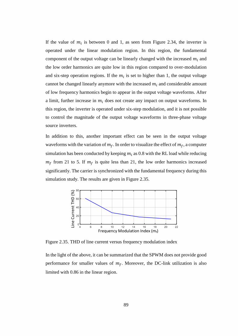
89

If the value of 𝑚𝑖 is between 0 and 1, as seen from Figure 2.34, the inverter is

operated under the linear modulation region. In this region, the fundamental

component of the output voltage can be linearly changed with the increased 𝑚𝑖 and

the low order harmonics are quite low in this region compared to over-modulation

and six-step operation regions. If the 𝑚𝑖 is set to higher than 1, the output voltage

cannot be changed linearly anymore with the increased 𝑚𝑖 and considerable amount

of low frequency harmonics begin to appear in the output voltage waveforms. After

a limit, further increase in 𝑚𝑖 does not create any impact on output waveforms. In

this region, the inverter is operated under six-step modulation, and it is not possible

to control the magnitude of the output voltage waveforms in three-phase voltage

source inverters.

In addition to this, another important effect can be seen in the output voltage

waveforms with the variation of 𝑚𝑓. In order to visualize the effect of 𝑚𝑓, a computer

simulation has been conducted by keeping 𝑚𝑖 as 0.8 with the RL load while reducing

𝑚𝑓 from 21 to 5. If 𝑚𝑓 is quite less than 21, the low order harmonics increased

significantly. The carrier is synchronized with the fundamental frequency during this

simulation study. The results are given in Figure 2.35.

Frequency Modulation Index (mf)

Lin

e C

urr

en

t TH

D (

%)

Figure 2.35. THD of line current versus frequency modulation index

In the light of the above, it can be summarized that the SPWM does not provide good

performance for smaller values of 𝑚𝑓. Moreover, the DC-link utilization is also

limited with 0.86 in the linear region.

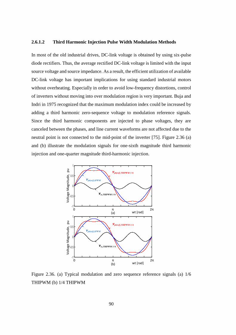
90

2.6.1.2 Third Harmonic Injection Pulse Width Modulation Methods

In most of the old industrial drives, DC-link voltage is obtained by using six-pulse

diode rectifiers. Thus, the average rectified DC-link voltage is limited with the input

source voltage and source impedance. As a result, the efficient utilization of available

DC-link voltage has important implications for using standard industrial motors

without overheating. Especially in order to avoid low-frequency distortions, control

of inverters without moving into over modulation region is very important. Buja and

Indri in 1975 recognized that the maximum modulation index could be increased by

adding a third harmonic zero-sequence voltage to modulation reference signals.

Since the third harmonic components are injected to phase voltages, they are

canceled between the phases, and line current waveforms are not affected due to the

neutral point is not connected to the mid-point of the inverter [75]. Figure 2.36 (a)

and (b) illustrate the modulation signals for one-sixth magnitude third harmonic

injection and one-quarter magnitude third-harmonic injection.

Vo

ltag

e M

agn

itu

de

, p

u

vph(ref),SPWM

vzs,THIPWM 1/4

vph(ref),THIPWM 1/4

wt [rad]2π 0 π

Vo

ltag

e M

agn

itu

de,

pu

vph(ref),SPWM

vzs,THIPWM 1/6

vph(ref),THIPWM 1/6

wt [rad]2π 0 π

(a)

(b)

Figure 2.36. (a) Typical modulation and zero sequence reference signals (a) 1/6

THIPWM (b) 1/4 THIPWM

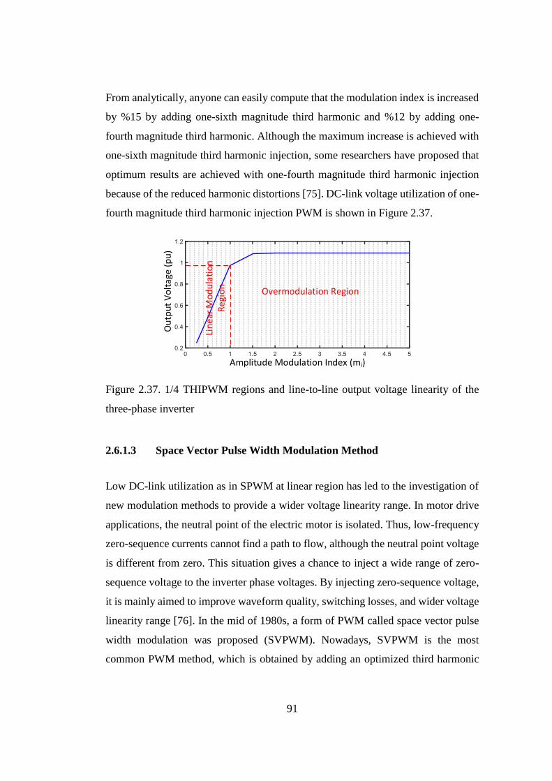
91

From analytically, anyone can easily compute that the modulation index is increased

by %15 by adding one-sixth magnitude third harmonic and %12 by adding one-

fourth magnitude third harmonic. Although the maximum increase is achieved with

one-sixth magnitude third harmonic injection, some researchers have proposed that

optimum results are achieved with one-fourth magnitude third harmonic injection

because of the reduced harmonic distortions [75]. DC-link voltage utilization of one-

fourth magnitude third harmonic injection PWM is shown in Figure 2.37.

Ou

tput

Vo

ltag

e (p

u)


Lin

ear

Mod

ula

tio

n

Reg

ion


Figure 2.37. 1/4 THIPWM regions and line-to-line output voltage linearity of the

three-phase inverter

2.6.1.3 Space Vector Pulse Width Modulation Method

Low DC-link utilization as in SPWM at linear region has led to the investigation of

new modulation methods to provide a wider voltage linearity range. In motor drive

applications, the neutral point of the electric motor is isolated. Thus, low-frequency

zero-sequence currents cannot find a path to flow, although the neutral point voltage

is different from zero. This situation gives a chance to inject a wide range of zero-

sequence voltage to the inverter phase voltages. By injecting zero-sequence voltage,

it is mainly aimed to improve waveform quality, switching losses, and wider voltage

linearity range [76]. In the mid of 1980s, a form of PWM called space vector pulse

width modulation was proposed (SVPWM). Nowadays, SVPWM is the most

common PWM method, which is obtained by adding an optimized third harmonic

92

zero-sequence voltage to the phase voltages. In practice, analog and digital

implementation of SVPWM have been applied. One of the simplest implementations

is that the reference modulation signals are generated by selecting the purely

sinusoidal modulation signal with the smallest magnitude and adding half of it to the

original sinusoidal reference signal [76]. Figure 2.38 shows the modulation signal

and third harmonic zero sequence component.

Vo

ltag

e M

agn

itu

de

, p

u

vph(ref),SPWM

vzs,SVPWM

vph(ref),SVPWM

wt [rad]2π 0 π

Figure 2.38. SPWM, SVPWM, and zero sequence signals

DC-link voltage utilization of SVPWM is illustrated in Figure 2.39. The SVPWM

method has a wider voltage linearity range comparing the other CPWM techniques

[76].

Ou

tpu

t V

olt

age

(p

u)


Lin

ear

Mo

du

lati

on

R

egi

on


Figure 2.39. SVPWM regions and line-to-line output voltage linearity of the three-

phase inverter

93

2.6.1.4 Discontinuous Pulse Width Modulation Methods

In the previous PWM methods, the reference modulation signals are always within

the carrier signal boundaries in the linear regions, and therefore, in every carrier

cycle, an on/off switching transition occurs. These methods are categorized as

Continuous PWM (CPWM) methods due to this continuous switching operation. In

the Discontinuous PWM (DPWM) methods, one semiconductor switch of each leg

is always turned-on during its 120º, 60º, or 30º unmodulated region, while the other

semiconductor switch of this leg is turned-off. These DPWM methods have the

advantage of eliminating switching transitions during some carrier periods. There

are six different DPWM methods, namely, DPWM0, DPWM1, DPWM2, DPWM3,

DPWMMIN, and DPWMMAX. All these DPWM methods have different

characteristics and provide different advantages. Therefore, choosing the correct

type is very important for the application. DPWM1 has minimum switching losses

at unity power factor operating conditions, while DPWM2 is suitable for lagging

power factor operating conditions. DPWM2 has minimum switching losses at 30°

lagging power factor. On the other hand, DPWM1 is the correct choice for leading

power factor operating conditions, and it has minimum switching losses for at 30°

leading power factor. In addition to this, DPWM3 provides the benefit of low

harmonic distortion. DPWMMAX and DPWMMIN give the benefits of low

harmonic distortion. However, the thermal stresses on semiconductors are non-

uniform. DPWM2 is sometimes useful for high power induction machine drives

because of the high semiconductor losses created with CPWM techniques. Because

of this, in accordance with the subject of the study, only waveforms related to

DPWM2 will be included. The modulation reference, phase voltages, line-to-line

output voltage, and line current waveforms are given in Figure 2.40 and Figure 2.41

at mi=0.905, fc=1050 Hz, and fm=50 Hz.

94

-1

-0.5

0

0.5

1

Time

Vo

ltag

e M

agn

itu

de

, p

uvAn(ref) vCn(ref)vBn(ref)


l-to-l voltage output at fm = 50 Hz when Vdc = 750 V.

Carrier signals, its frequency is fc = 1050 Hz for illustration.

0

Time

1

VA,

pu

0

Time

1

VB,

pu

0

Time

1

VC,

pu

0

Time

1

VA

B,

pu

-1

(a)

(b)

(c)

(d)

(e)

Figure 2.40. Typical voltage waveforms for DPWM2 modulated two-level voltage

source inverter (a) Modulation and carrier signals (b) - (d) Phase voltages (e) Line-

to-line output voltage

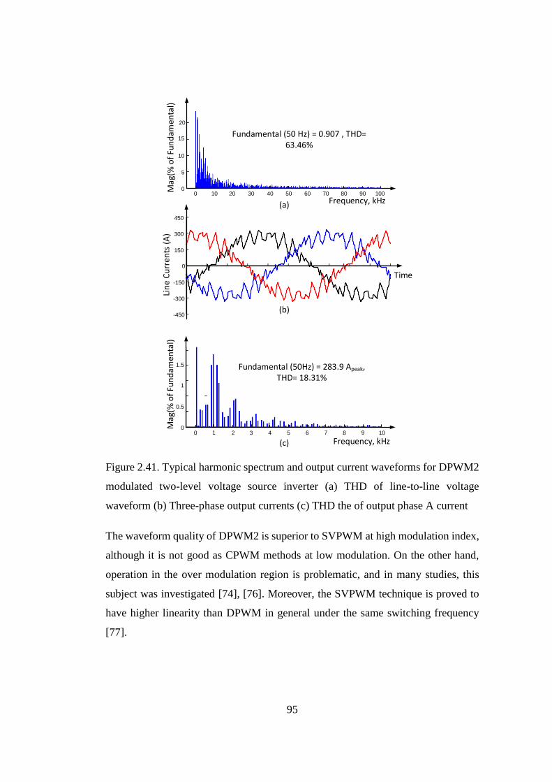
95

Fundamental (50 Hz) = 0.907 , THD= 63.46%

Mag

(% o

f Fu

nd

amen

tal)

Frequency, kHz0 10

0

20

15

10

5

20 30 40 50 60 70 80 90 100

0

Time

300

Lin

e C

urr

ents

(A

)

-450

150

-150

-300

450

0

Frequency, kHz

Mag

(% o

f Fu

nd

amen

tal)

0 2 4 6 8 10

1.5

1

0.5

Fundamental (50Hz) = 283.9 Apeak, THD= 18.31%

97531

(a)

(b)

(c)

Figure 2.41. Typical harmonic spectrum and output current waveforms for DPWM2

modulated two-level voltage source inverter (a) THD of line-to-line voltage

waveform (b) Three-phase output currents (c) THD the of output phase A current

The waveform quality of DPWM2 is superior to SVPWM at high modulation index,

although it is not good as CPWM methods at low modulation. On the other hand,

operation in the over modulation region is problematic, and in many studies, this

subject was investigated [74], [76]. Moreover, the SVPWM technique is proved to

have higher linearity than DPWM in general under the same switching frequency

[77].

96

2.6.1.5 Programmed Pulse Width Modulation Methods

In high power traction applications, overall system efficiency is very important.

Therefore, the switching and harmonic losses have to be considered to reduce

operational cost and the thermal stresses (e.g., longer life time and higher operational

system efficiency). Due to these reasons, the switching frequencies of IGBTs are

limited in the range of 500-3000 Hz. For lower switching frequencies, 𝑚𝑓 is getting

very low, especially in high-speed operation regions. This reduces the resolution in

PWM patterns, may lead to loss of full-wave, half-wave, and quarter-wave waveform

symmetricity. As a result of that, low order (5th, 7th, 11th, 13th, 17th, etc.) frequency

harmonics are generated in the output waveforms. In practice, low-frequency

harmonic components cannot be filtered by using small passive filters. In this case,

the filter increases the product size, weight, and system cost. Because of this reason,

bulky low pass filters are not preferred in traction applications. In addition to this,

many studies show that multilevel converters have been providing good performance

to decrease the harmonics in high power applications. However, this also increases

the cost and decreases the reliability of the converter because of the increased

number of semiconductors, gate-drives, capacitors, isolated power supplies, and so

on. On the other hand, different PWM techniques may also help to manage low order

harmonics up to a certain level. Instead of carrier-based PWM methods, three major

programmed PWM methods, namely Selective Harmonic Elimination PWM,

Selective Harmonic Mitigation PWM, and Synchronous Optimal PWM, are used to

eliminate the low order frequency harmonics in practice [75], [78]–[80]. The use of

these efficient modulation methods will be very convenient to obtain output

waveforms with acceptable harmonic content in high-power applications. The

approach of these modulation methods is based on the cancellation of low order

current harmonics or the minimization of the RMS value of the current harmonics in

the motor by a proper choice of the commutation angles by taking into account

suitable objective functions [78].

97

By using the SHEPWM method, a limited number of low-order harmonics can be

canceled. However, the non-canceled and relatively high order harmonics are not

controlled. On the other hand, the SHMPWM method gives a chance to reduce the

magnitudes of low order and high order harmonics altogether. The main goal of this

modulation method is to reduce the filtering requirements in order to decrease the

size, weight, and cost of the filtering elements by fulfilling the harmonic

requirements [80]. In addition to this, Buja and Indri [81] proposed the SOPWM

method, which considers a whole spectrum to minimize the harmonic distortion of

the current in a motor.

In all these methods, the pulse angles have to be calculated by solving idealized

analytical formulations. In practice, the complexity of the problem increases as the

number of switching angles increases; finding the optimum solutions are getting

harder, and the switching losses increase, although using more switching angles

eliminates more harmonics. In order to solve a set of analytical formulations, there

have been two groups of techniques presented in the literature, namely iterative

solution and search algorithm techniques. Almost all of these techniques require

heavy computational effort. Because of this difficulty, the angles have been solved

with offline calculations and stored in lookup tables. However, in practice, this

approach is not easily applicable for traction applications where the electrification

line voltage is not fix. In order to optimize the harmonics, line voltage fluctuations

have to be considered. All of the angles should be solved by considering many

conditions (different modulation indexes, pulse numbers, etc.) and stored in the

lookup tables. This creates big problems. In order to overcome these problems,

online calculation of pulse angles can be done. Online calculations can be made by

using a graphical processing unit that provides high-level computing technology.

However, the system and labor cost increase a lot in this case.

98

2.7 Principles of Electric Traction Drives

The high-performance electric traction drive systems should offer the following

features:

• four-quadrant operation,

• high power density,

• high conversion efficiency,

• fast-flux and torque response,

• fast dynamics for slip/slide protection,

• maximum output torque per ampere operation in wide speed range,

• high and constant switching frequency,

• high current control bandwidth,

• robustness to parameter variations,

• high reliability and low maintenance need,

• low cost,

• low flux and torque ripple,

• low current harmonic distortion for motor currents.

Hardware capabilities and applied control strategy should be considered together to

provide the above-listed features. DC-link voltage, phase currents, modulation index

mi, slip, and rotor frequency are the important parameters for induction machine

control. These may differ according to the applied motor control algorithms.

99

2.7.1 Control Methods for Voltage Source Inverter Fed Induction

Machines in Railway Applications

In this section, control methods for voltage source inverter fed induction machine

drive will be presented. This section has been performed with two main goals:

presenting the theoretical background of each control method and comparative

analysis and choosing the most appropriate control methods considering the

operating regions.

Traction converters commonly receive a torque command from the master controller

or CBCT/ERTMS systems. The applicable torque that can be produced at a given

speed will essentially depend on the machine and inverter designs, as explained in

this section. The operating regions as constant torque, constant power, and high-

speed regions are defined. The traction inverters are responsible for driving induction

machines properly in all these regions. The gain and phase margins are very

important for stable motor control. The stability of such drives depends on available

voltage, applicable switching frequency, applied control method, and modulation

technique. In fact, all of these also dynamically depend on each other. Therefore,

control method, modulation technique, switching frequency, and available voltage

should be considered altogether for an efficient and stable traction drive system.

Even for most of the medium-power drives, control methods, modulation techniques,

and switching frequency are changed dynamically depending on the operating region

of the traction motors.

Control methods for induction machines can be classified as scalar and vector types.

Scalar control methods are derived from the steady-state equivalent machine models

and are suitable for applications that do not require very fast changes in operating

conditions. Vector control methods are contrarily used for high-performance drives,

which require fast control loops and dynamic responses. Instead of steady-state

equations, dynamic equations of the machine are used in this case. The upper-level

block diagram of induction machine control methods is illustrated in Figure 2.42

[58].

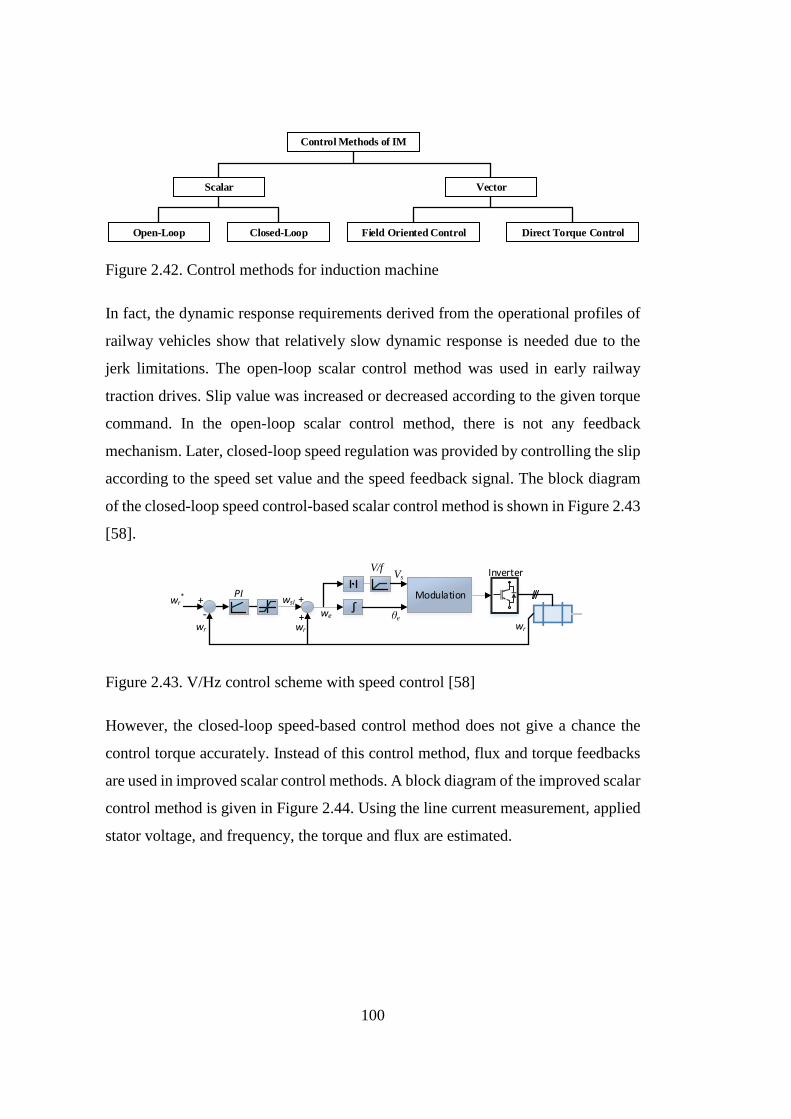
100

Control Methods of IM

VectorScalar

Field Oriented Control Direct Torque ControlOpen-Loop Closed-Loop

Figure 2.42. Control methods for induction machine

In fact, the dynamic response requirements derived from the operational profiles of

railway vehicles show that relatively slow dynamic response is needed due to the

jerk limitations. The open-loop scalar control method was used in early railway

traction drives. Slip value was increased or decreased according to the given torque

command. In the open-loop scalar control method, there is not any feedback

mechanism. Later, closed-loop speed regulation was provided by controlling the slip

according to the speed set value and the speed feedback signal. The block diagram

of the closed-loop speed control-based scalar control method is shown in Figure 2.43

[58].

+

-ʃ

Modulationwr*

wr

PI+

+wr

we θe

Vs

V/f Inverter

wr

wsl

Figure 2.43. V/Hz control scheme with speed control [58]

However, the closed-loop speed-based control method does not give a chance the

control torque accurately. Instead of this control method, flux and torque feedbacks

are used in improved scalar control methods. A block diagram of the improved scalar

control method is given in Figure 2.44. Using the line current measurement, applied

stator voltage, and frequency, the torque and flux are estimated.

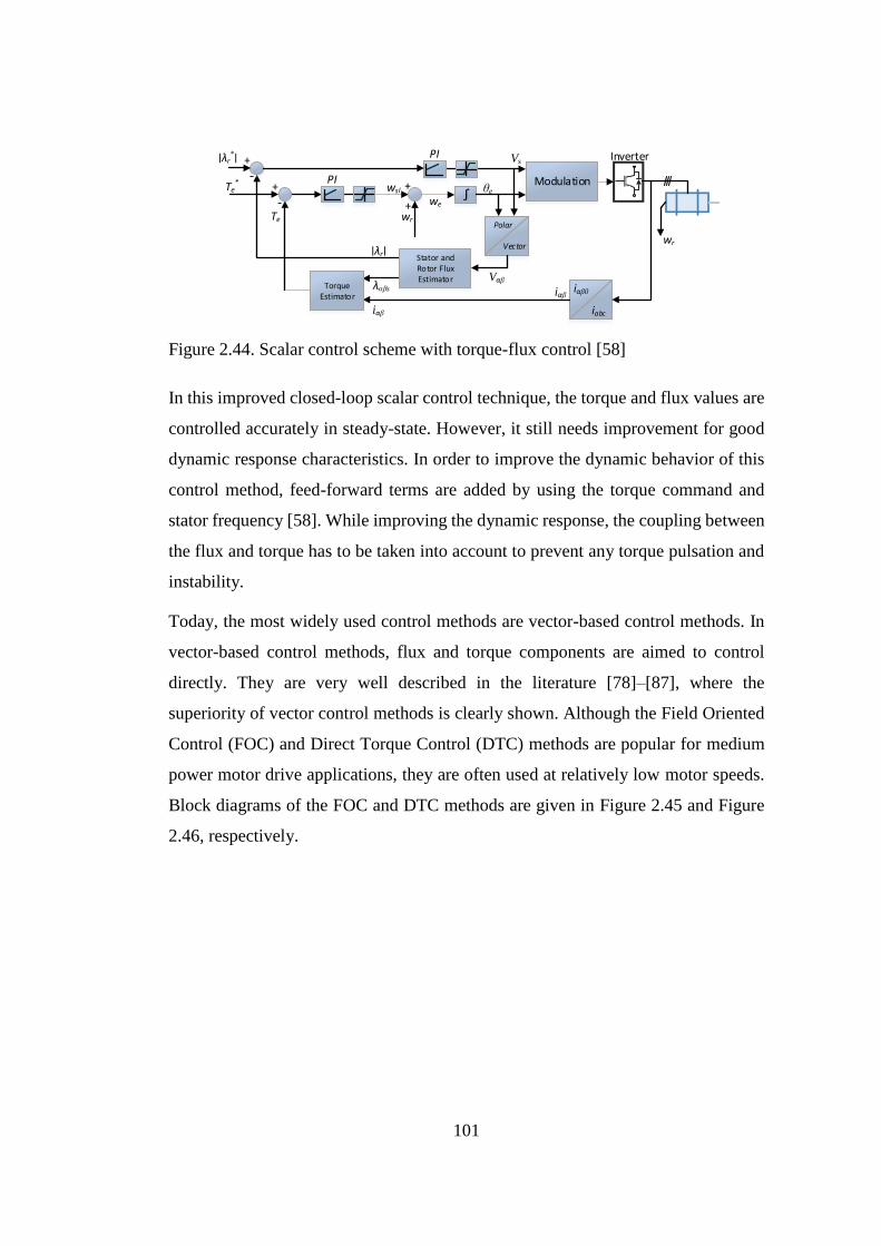
101

+

-ʃ

ModulationTe*

Te

PI+

+wr

we

θe

VsInverter

wr

Polar

Vector

Vαβ

iαβ0

iabc

iαβ

Stator and Rotor Flux Estimator

Torque Estimator

PI

wsl

iαβ

λαβs

λr

+

-

λr*

Figure 2.44. Scalar control scheme with torque-flux control [58]

In this improved closed-loop scalar control technique, the torque and flux values are

controlled accurately in steady-state. However, it still needs improvement for good

dynamic response characteristics. In order to improve the dynamic behavior of this

control method, feed-forward terms are added by using the torque command and

stator frequency [58]. While improving the dynamic response, the coupling between

the flux and torque has to be taken into account to prevent any torque pulsation and

instability.

Today, the most widely used control methods are vector-based control methods. In

vector-based control methods, flux and torque components are aimed to control

directly. They are very well described in the literature [78]–[87], where the

superiority of vector control methods is clearly shown. Although the Field Oriented

Control (FOC) and Direct Torque Control (DTC) methods are popular for medium

power motor drive applications, they are often used at relatively low motor speeds.

Block diagrams of the FOC and DTC methods are given in Figure 2.45 and Figure

2.46, respectively.

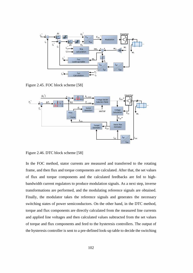
102

+

- Modulation

iq*

iq

PIVabc

*Inverter

wr

idref

Look-up table

Vdq

Vabc

iαβ

iabc

idq

iαβ

+

-id

PIid*

Vq*

Vd*

wr

ppwreSlip

calculation

iq*

id*

swe + +

ʃ

θe

weid*

iqref

Calculation

Te*

idiq

*

Figure 2.45. FOC block scheme [58]

+

-

Voltage Vector Selection TableTe

*

Te

Inverter

wr

Vαβ*

iαβ

Stator Flux Estimator

Torque Estimator λαβs

+

-

λs*

Sabc*

Voltage Calculation

iαβ

iabc

Vdc

iabc

Polar

Vector

Sector Detection

λs_state

Te_state10

-1

1

0

λαβs

θs

λs ΔTe

sector

Figure 2.46. DTC block scheme [58]

In the FOC method, stator currents are measured and transferred to the rotating

frame, and then flux and torque components are calculated. After that, the set values

of flux and torque components and the calculated feedbacks are fed to high-

bandwidth current regulators to produce modulation signals. As a next step, inverse

transformations are performed, and the modulating reference signals are obtained.

Finally, the modulator takes the reference signals and generates the necessary

switching states of power semiconductors. On the other hand, in the DTC method,

torque and flux components are directly calculated from the measured line currents

and applied line voltages and then calculated values subtracted from the set values

of torque and flux components and feed to the hysteresis controllers. The output of

the hysteresis controller is sent to a pre-defined look-up table to decide the switching

103

states of power semiconductors. This control method is not suitable for operation at

the boundary of the overmodulation region. In addition to this, it is difficult to keep

the switching frequency constant. Hence, it is not preferred in high-power railway

traction drives [58].

Moreover, due to the increased output fundamental frequency, the switching

frequency to fundamental voltage-frequency ratio is decreased with increased speed.

This causes to generates lower-order voltage harmonics hence current harmonics,

and leads to decrease system efficiency and stability. In order to solve this problem,

different modulation techniques, such as SHEPWM, SHMPWM, and OPWM with

scalar motor control methods, have to be applied.

Consequently, the use of vector-based control methods in railway applications at

high speeds can be problematic due to the insufficient voltage margin, limited

switching frequency, and unsuitability for use with SHEPWM, SHMPWM, and

OPWM techniques. In over modulation regions, the current and voltage distortions

became prominent. This situation causes instability problems. On the other hand,

V/Hz control methods are fitted well with these modulation techniques for high-

speed operating regions, although the dynamic performance is poor. All these

explain that why the control methods and modulation techniques are dependent on

operating regions. In order to overcome the disadvantages of control methods and

modulation techniques in all operating region, the use of a mix of control methods

and modulation techniques are preferred. At relatively low speeds, the FOC method

and SVPWM techniques can be used. While this is the case for low speed (e.g.,

generally is limited with constant torque region), the V/Hz control method can be

used together with one of the above-mentioned preprogrammed modulation

techniques for constant power and high-speed regions. Table 2.8 summarizes the

properties of control methods [58]. It is also worthy to note that torque command

step changes are normally limited in railway applications due to the jerk limitation,

which is required for passenger comfort. Instead of this, the traction drive has to meet

the acceptable torque/current ripple requirements.

104

Table 2.8 Summary of Presented Control Methods for Railway Traction

Control Methods

Properties

Open-Loop Closed-Loop

V/Hz

V/Hz with

only speed

feedback

V/Hz with speed

and current

feedbacks

Rotor flux

oriented

control

Direct

torque

control

Reference frame rotating rotating rotating rotating stationary

Fix switching

frequency yes yes yes yes no

Low speed

performance modarate modarate modarate good poor

High speed

(overmodulation)

performance

good good good moderate poor

Six-step

operation good good good

needs additional

improvement

Dynamic

response poor poor moderate good good

As explained above, the main source of the problem is the applicable low switching

frequencies at high speeds. This picture began to change with the discovery of SiC

power semiconductors. Hereafter, the traction drive systems using FOC control and

SVPWM modulation techniques, which are almost the only solution in low power

applications, will be possible instead of mixed control and modulation methods that

switch between each other for medium power and medium voltage applications.

105

CHAPTER 3

3 DESIGN AND IMPLEMENTATION OF ALL SIC TRACTION INVERTER

The architecture of electric traction systems, brief information about traction motors,

traction inverter topologies, and operating principles have been presented in Chapter

2. It was also emphasized that the traction inverters must perform high-performance

tasks in harsh environmental conditions. In this chapter, the design methodology and

implementation of a high-performance 500 – 900 VDC, 165 kVA all SiC traction

inverter prototype is presented.

3.1 Design Methodology of Prototype System

Within the scope of this thesis, the prototype of a full SiC-based traction inverter has

been designed, developed, and verified. To be able to define traction system

requirements, traction analysis is firstly performed. Type of electrification system,

the diameter of the vehicle wheel, the empty and fully-loaded weight of the vehicle,

track data and acceleration/deceleration specifications are taken into account and

then, voltage and current ratings of traction inverter and traction motor, and turns

ratio of the gearbox are determined.

Light rail transportation systems are usually operating in the form of a vehicle set

consisting of multiple cars. They run under very severe operating conditions of tight

curves and frequent acceleration and braking. Generally, they are powered by 750

VDC electrification systems. The vehicles have maximum operating speeds of about

50-80km/h.

The flow chart of the proposed systematic design approach is shown in Figure 3.1.

It starts by collecting the system requirements and doing traction analysis. Then, a

proper inverter topology is chosen according to derived requirements. Switching

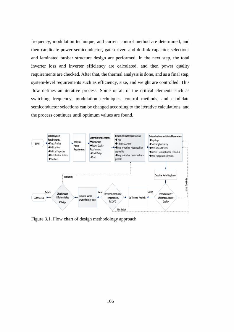
106

frequency, modulation technique, and current control method are determined, and

then candidate power semiconductor, gate-driver, and dc-link capacitor selections

and laminated busbar structure design are performed. In the next step, the total

inverter loss and inverter efficiency are calculated, and then power quality

requirements are checked. After that, the thermal analysis is done, and as a final step,

system-level requirements such as efficiency, size, and weight are controlled. This

flow defines an iterative process. Some or all of the critical elements such as

switching frequency, modulation techniques, control methods, and candidate

semiconductor selections can be changed according to the iterative calculations, and

the process continues until optimum values are found.

Check Converter Efficiency & Power

Quality

Collect System RequirementsTrack ProfilesVehicle DutyVehicle PropertiesElectrification SystemsStandards

Analysize Power Requirements

Determine Main AspecsBandwidthPower Quality RequirementsSize&WeightCost

Calculate Switching Losses

No

t S

atis

fy

Do Thermal AnalysisCheck Semiconductor

Temperatures, Tj 120°C

Not Satisfy

Calculate Motor Drive Efficiency Map

Check System Efficiency&Size

&Weight

Determine Motor SpecificationTypeVoltage&CurrentKeep motor line voltage as high as possibleKeep motor line current as low as possible

Not Satisfy

START

COMPLETED

Determine Inverter Related ParametersTopologySwitching FrequencyModulation MehodsCurrent (Torque) Control TechniqueMain component selections

SatisfySatisfySatisfy

Figure 3.1. Flow chart of design methodology approach

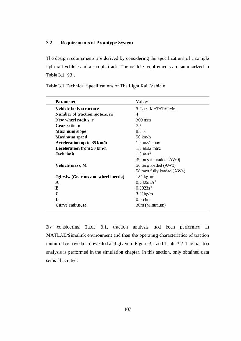
107

3.2 Requirements of Prototype System

The design requirements are derived by considering the specifications of a sample

light rail vehicle and a sample track. The vehicle requirements are summarized in

Table 3.1 [93].

Table 3.1 Technical Specifications of The Light Rail Vehicle

Parameter Values

Vehicle body structure 5 Cars, M+T+T+T+M

Number of traction motors, m 4

New wheel radius, r 300 mm

Gear ratio, n 7.5

Maximum slope 8.5 %

Maximum speed 50 km/h

Acceleration up to 35 km/h 1.2 m/s2 max.

Deceleration from 50 km/h 1.3 m/s2 max.

Jerk limit 1.0 m/s3

Vehicle mass, M

39 tons unloaded (AW0)

56 tons loaded (AW3)

58 tons fully loaded (AW4)

Jgb+Jw (Gearbox and wheel inertia) 182 kg-m2

A

B

C

D

Curve radius, R

0.0405m/s2

0.0023s-1

3.81kg/m

0.053m

30m (Minimum)

By considering Table 3.1, traction analysis had been performed in

MATLAB/Simulink environment and then the operating characteristics of traction

motor drive have been revealed and given in Figure 3.2 and Table 3.2. The traction

analysis is performed in the simulation chapter. In this section, only obtained data

set is illustrated.

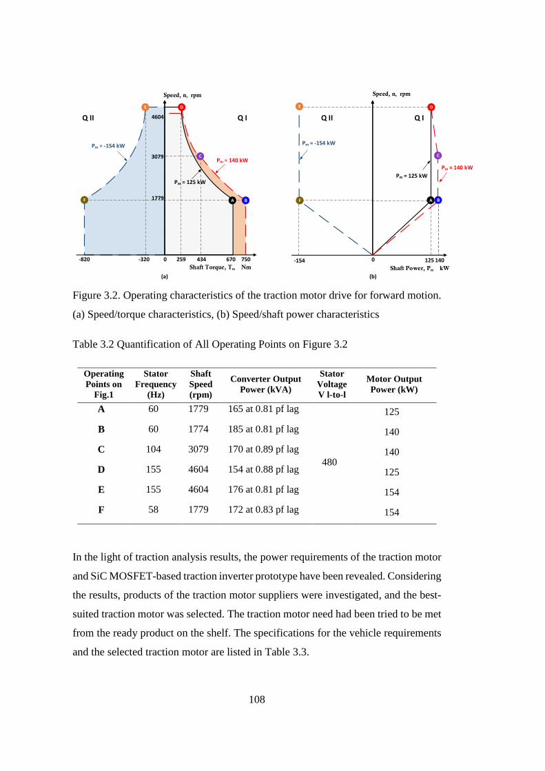
108

0

A

750670

Pm = 140 kW

Pm = 125 kW

B

C

F

-820

Pm = -154 kW

-320 434259

DE

Speed, nr rpm

1779

3079

4604 Q IQ II

Shaft Torque, Tm Nm

0 140125-154

Speed, nr rpm

Shaft Power, Pm kW

F A B

D

C

E

Pm = -154 kW

Pm = 140 kW

Pm = 125 kW

Q IQ II

(a) (b)

Figure 3.2. Operating characteristics of the traction motor drive for forward motion.

(a) Speed/torque characteristics, (b) Speed/shaft power characteristics

Table 3.2 Quantification of All Operating Points on Figure 3.2

Operating

Points on

Fig.1

Stator

Frequency

(Hz)

Shaft

Speed

(rpm)

Converter Output

Power (kVA)

Stator

Voltage

V l-to-l

Motor Output

Power (kW)

A 60 1779 165 at 0.81 pf lag

480

125

B 60 1774 185 at 0.81 pf lag 140

C 104 3079 170 at 0.89 pf lag 140

D 155 4604 154 at 0.88 pf lag 125

E 155 4604 176 at 0.81 pf lag 154

F 58 1779 172 at 0.83 pf lag 154

In the light of traction analysis results, the power requirements of the traction motor

and SiC MOSFET-based traction inverter prototype have been revealed. Considering

the results, products of the traction motor suppliers were investigated, and the best-

suited traction motor was selected. The traction motor need had been tried to be met

from the ready product on the shelf. The specifications for the vehicle requirements

and the selected traction motor are listed in Table 3.3.

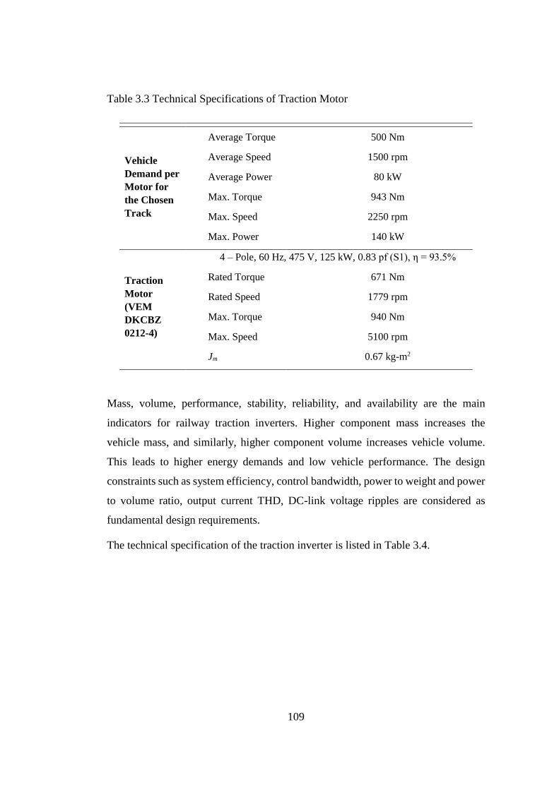
109

Table 3.3 Technical Specifications of Traction Motor

Vehicle

Demand per

Motor for

the Chosen

Track

Average Torque 500 Nm

Average Speed 1500 rpm

Average Power 80 kW

Max. Torque 943 Nm

Max. Speed 2250 rpm

Max. Power 140 kW

Traction

Motor

(VEM

DKCBZ

0212-4)

4 – Pole, 60 Hz, 475 V, 125 kW, 0.83 pf (S1), η = 93.5%

Rated Torque 671 Nm

Rated Speed 1779 rpm

Max. Torque 940 Nm

Max. Speed

Jm

5100 rpm

0.67 kg-m2

Mass, volume, performance, stability, reliability, and availability are the main

indicators for railway traction inverters. Higher component mass increases the

vehicle mass, and similarly, higher component volume increases vehicle volume.

This leads to higher energy demands and low vehicle performance. The design

constraints such as system efficiency, control bandwidth, power to weight and power

to volume ratio, output current THD, DC-link voltage ripples are considered as

fundamental design requirements.

The technical specification of the traction inverter is listed in Table 3.4.

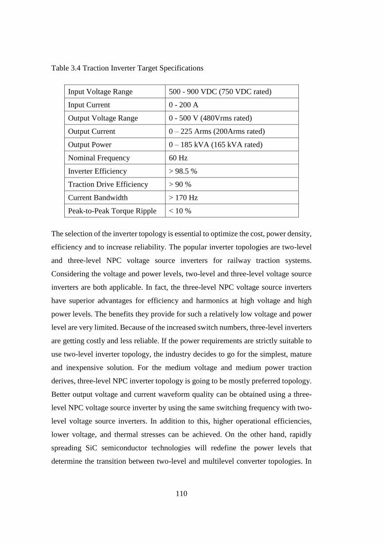
110

Table 3.4 Traction Inverter Target Specifications

Input Voltage Range 500 - 900 VDC (750 VDC rated)

Input Current 0 - 200 A

Output Voltage Range 0 - 500 V (480Vrms rated)

Output Current 0 – 225 Arms (200Arms rated)

Output Power 0 – 185 kVA (165 kVA rated)

Nominal Frequency 60 Hz

Inverter Efficiency > 98.5 %

Traction Drive Efficiency > 90 %

Current Bandwidth > 170 Hz

Peak-to-Peak Torque Ripple < 10 %

The selection of the inverter topology is essential to optimize the cost, power density,

efficiency and to increase reliability. The popular inverter topologies are two-level

and three-level NPC voltage source inverters for railway traction systems.

Considering the voltage and power levels, two-level and three-level voltage source

inverters are both applicable. In fact, the three-level NPC voltage source inverters

have superior advantages for efficiency and harmonics at high voltage and high

power levels. The benefits they provide for such a relatively low voltage and power

level are very limited. Because of the increased switch numbers, three-level inverters

are getting costly and less reliable. If the power requirements are strictly suitable to

use two-level inverter topology, the industry decides to go for the simplest, mature

and inexpensive solution. For the medium voltage and medium power traction

derives, three-level NPC inverter topology is going to be mostly preferred topology.

Better output voltage and current waveform quality can be obtained using a three-

level NPC voltage source inverter by using the same switching frequency with two-

level voltage source inverters. In addition to this, higher operational efficiencies,

lower voltage, and thermal stresses can be achieved. On the other hand, rapidly

spreading SiC semiconductor technologies will redefine the power levels that

determine the transition between two-level and multilevel converter topologies. In

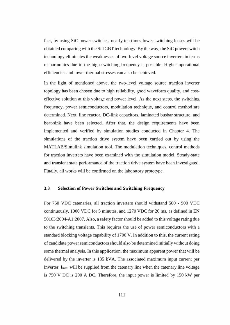
111

fact, by using SiC power switches, nearly ten times lower switching losses will be

obtained comparing with the Si-IGBT technology. By the way, the SiC power switch

technology eliminates the weaknesses of two-level voltage source inverters in terms

of harmonics due to the high switching frequency is possible. Higher operational

efficiencies and lower thermal stresses can also be achieved.

In the light of mentioned above, the two-level voltage source traction inverter

topology has been chosen due to high reliability, good waveform quality, and cost-

effective solution at this voltage and power level. As the next steps, the switching

frequency, power semiconductors, modulation technique, and control method are

determined. Next, line reactor, DC-link capacitors, laminated busbar structure, and

heat-sink have been selected. After that, the design requirements have been

implemented and verified by simulation studies conducted in Chapter 4. The

simulations of the traction drive system have been carried out by using the

MATLAB/Simulink simulation tool. The modulation techniques, control methods

for traction inverters have been examined with the simulation model. Steady-state

and transient state performance of the traction drive system have been investigated.

Finally, all works will be confirmed on the laboratory prototype.

3.3 Selection of Power Switches and Switching Frequency

For 750 VDC catenaries, all traction inverters should withstand 500 - 900 VDC

continuously, 1000 VDC for 5 minutes, and 1270 VDC for 20 ms, as defined in EN

50163:2004-A1:2007. Also, a safety factor should be added to this voltage rating due

to the switching transients. This requires the use of power semiconductors with a

standard blocking voltage capability of 1700 V. In addition to this, the current rating

of candidate power semiconductors should also be determined initially without doing

some thermal analysis. In this application, the maximum apparent power that will be

delivered by the inverter is 185 kVA. The associated maximum input current per

inverter, Imax, will be supplied from the catenary line when the catenary line voltage

is 750 V DC is 200 A DC. Therefore, the input power is limited by 150 kW per

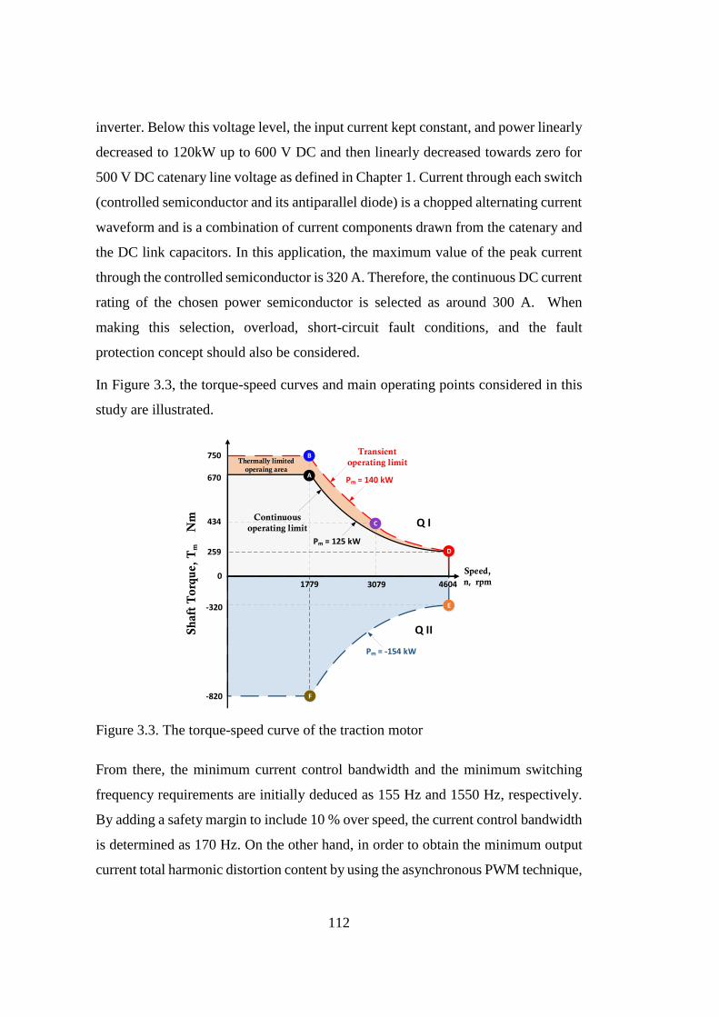
112

inverter. Below this voltage level, the input current kept constant, and power linearly

decreased to 120kW up to 600 V DC and then linearly decreased towards zero for

500 V DC catenary line voltage as defined in Chapter 1. Current through each switch

(controlled semiconductor and its antiparallel diode) is a chopped alternating current

waveform and is a combination of current components drawn from the catenary and

the DC link capacitors. In this application, the maximum value of the peak current

through the controlled semiconductor is 320 A. Therefore, the continuous DC current

rating of the chosen power semiconductor is selected as around 300 A. When

making this selection, overload, short-circuit fault conditions, and the fault

protection concept should also be considered.

In Figure 3.3, the torque-speed curves and main operating points considered in this

study are illustrated.

0

A

750

670 Pm = 140 kW

Pm = 125 kW

B

C

F-820

Pm = -154 kW

-320

434

259 D

E

Speed,

nr rpm1779 3079 4604

Q I

Sh

aft

To

rqu

e, T

m

Nm

Q II

Continuous

operating limit

Transient

operating limitThermally limited

operaing area

Figure 3.3. The torque-speed curve of the traction motor

From there, the minimum current control bandwidth and the minimum switching

frequency requirements are initially deduced as 155 Hz and 1550 Hz, respectively.

By adding a safety margin to include 10 % over speed, the current control bandwidth

is determined as 170 Hz. On the other hand, in order to obtain the minimum output

current total harmonic distortion content by using the asynchronous PWM technique,

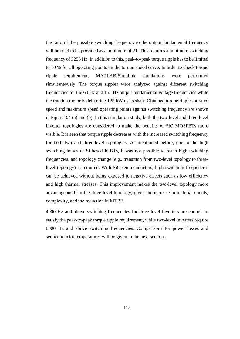
113

the ratio of the possible switching frequency to the output fundamental frequency

will be tried to be provided as a minimum of 21. This requires a minimum switching

frequency of 3255 Hz. In addition to this, peak-to-peak torque ripple has to be limited

to 10 % for all operating points on the torque-speed curve. In order to check torque

ripple requirement, MATLAB/Simulink simulations were performed

simultaneously. The torque ripples were analyzed against different switching

frequencies for the 60 Hz and 155 Hz output fundamental voltage frequencies while

the traction motor is delivering 125 kW to its shaft. Obtained torque ripples at rated

speed and maximum speed operating points against switching frequency are shown

in Figure 3.4 (a) and (b). In this simulation study, both the two-level and three-level

inverter topologies are considered to make the benefits of SiC MOSFETs more

visible. It is seen that torque ripple decreases with the increased switching frequency

for both two and three-level topologies. As mentioned before, due to the high

switching losses of Si-based IGBTs, it was not possible to reach high switching

frequencies, and topology change (e.g., transition from two-level topology to three-

level topology) is required. With SiC semiconductors, high switching frequencies

can be achieved without being exposed to negative effects such as low efficiency

and high thermal stresses. This improvement makes the two-level topology more

advantageous than the three-level topology, given the increase in material counts,

complexity, and the reduction in MTBF.

4000 Hz and above switching frequencies for three-level inverters are enough to

satisfy the peak-to-peak torque ripple requirement, while two-level inverters require

8000 Hz and above switching frequencies. Comparisons for power losses and

semiconductor temperatures will be given in the next sections.

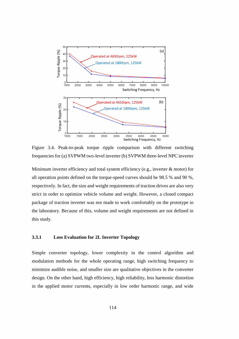
114

Torq

ue

Rip

ple

(%

)

Switching Frequency, Hz

Operated at 4650rpm, 125kW


(b)

Torq

ue

Rip

ple

(%

)

Switching Frequency, Hz



(a)

Figure 3.4. Peak-to-peak torque ripple comparison with different switching

frequencies for (a) SVPWM two-level inverter (b) SVPWM three-level NPC inverter

Minimum inverter efficiency and total system efficiency (e.g., inverter & motor) for

all operation points defined on the torque-speed curves should be 98.5 % and 90 %,

respectively. In fact, the size and weight requirements of traction drives are also very

strict in order to optimize vehicle volume and weight. However, a closed compact

package of traction inverter was not made to work comfortably on the prototype in

the laboratory. Because of this, volume and weight requirements are not defined in

this study.

3.3.1 Loss Evaluation for 2L Inverter Topology

Simple converter topology, lower complexity in the control algorithm and

modulation methods for the whole operating range, high switching frequency to

minimize audible noise, and smaller size are qualitative objectives in the converter

design. On the other hand, high efficiency, high reliability, less harmonic distortion

in the applied motor currents, especially in low order harmonic range, and wide

115

current and hence torque bandwidth are being the quantitative design objectives. In

the design phase, the traction converter, which optimizes not only the initial cost/kW-

converter but also the operating cost (lower energy consumption, less maintenance),

should be preferred.

Two-level classical three-phase bridge topology without parallel or series-connected

power semiconductors in all legs in conjunction with the most common space vector

PWM as the modulation technique and field-oriented control to adjust rotor flux

during operation meets some of the design objectives given above. To complete the

optimum design work, the most suitable types of power semiconductors among Si-

IGBT, hybrid IGBT, asymmetrical IGCT, and SiC Power MOSFET and the

optimum switching frequency for the chosen power semiconductor should be

determined by carrying out some computer simulations. In traction converters

supplied from 750 V DC catenary lines, asymmetrical IGCTs are not used because

of their very high current and voltage ratings suitable only for operating at 1500 and

3000 V DC-link voltages.

Commercially available candidate power semiconductors evaluated in this study are

given in Table 3.5. Note that the traction application compliant semiconductors were

not used in this study to find the comparable package, current, and voltage

specifications that are similar to the SiC MOSFET module.

116

Table 3.5 Technical Specifications of Candidate Semiconductors

Semiconductor Modules

Ratings

Si-IGBT

Infineon

FF300R17KE4

Si-IGBT

Mitsubishi

CM300DY-34T

Hybrid-IGBT

Fuji Electric

2MSI400VAE-170-53

SiC MOSFET

Wolfspeed/Cree

CAS300M17BM2

Max. Blocking Voltage (V) 1700 1700 1700 1700

Continues Current (A) @

25°C 440 300 520 325

Rdson /Vce(sat) 1.95V 1.95V 2.15 8 mOhm

Total Gate Charge (nC) 3050 2350 3000 1076

Recovery Charge (µC )

@125°C 105 105 almost 0 almost 0

Max. Junction Operating

Temp. (°C) 150 150 150 150

Base Area (mm2) 61.4x106.4 62x108 80x110 61.4x106.4

Thermal Resistance per

MOSFET/IGBT Junction-

to-case (K/kW)

40 44.0 33 67

Thermal Resistance per

Diode Junction-to-case

(K/kW)

65 67.7 70 60

Selection of the power switches and the switching frequency is a fundamental issue

for a power converter. Whole system performance is directly affected by this choice.

When selecting the power switches and the switching frequency for the traction

inverter, several practical issues should be considered. Traction motor current

harmonics, desired rotational speed of traction motor or current control bandwidth

of the inverter, system efficiency, modulation techniques, DC-link capacitor

currents, input harmonics, power switch thermal resistances, and the cooling system

requirements have to be considered for selection of power switches and switching

frequency. In addition to this, the characteristic of the power switch should be

identified very well since the power switch junction temperature depends on thermal

resistances and capacitances, conduction, and switching losses. The switching

frequency of the active switches is very important for output waveform quality.

Higher switching frequency is quite well in order to obtain better waveform quality;

however, it is limited with the semiconductor losses. In medium voltage and medium

power applications, the switching frequency cannot be kept higher than a few kHz

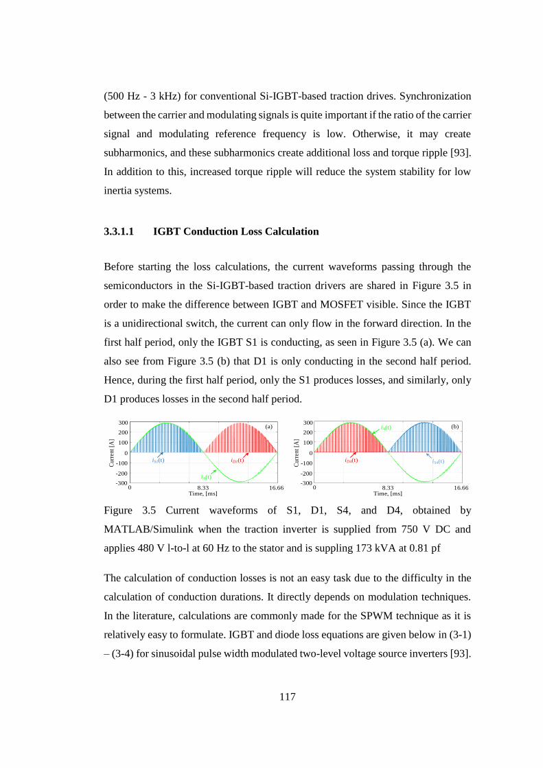
117

(500 Hz - 3 kHz) for conventional Si-IGBT-based traction drives. Synchronization

between the carrier and modulating signals is quite important if the ratio of the carrier

signal and modulating reference frequency is low. Otherwise, it may create

subharmonics, and these subharmonics create additional loss and torque ripple [93].

In addition to this, increased torque ripple will reduce the system stability for low

inertia systems.

3.3.1.1 IGBT Conduction Loss Calculation

Before starting the loss calculations, the current waveforms passing through the

semiconductors in the Si-IGBT-based traction drivers are shared in Figure 3.5 in

order to make the difference between IGBT and MOSFET visible. Since the IGBT

is a unidirectional switch, the current can only flow in the forward direction. In the

first half period, only the IGBT S1 is conducting, as seen in Figure 3.5 (a). We can

also see from Figure 3.5 (b) that D1 is only conducting in the second half period.

Hence, during the first half period, only the S1 produces losses, and similarly, only

D1 produces losses in the second half period.

Cu

rren

t [A

]

0

100

200

iA(t)

16.66Time, [ms]

iS1(t) iD1(t)

300

-100

-200

-3008.330

Cu

rren

t [A

]

0

100

200iA(t)

16.66Time, [ms]

iD4(t) iS4(t)

300

-100

-200

-3008.330

(a) (b)

Figure 3.5 Current waveforms of S1, D1, S4, and D4, obtained by


applies 480 V l-to-l at 60 Hz to the stator and is suppling 173 kVA at 0.81 pf

The calculation of conduction losses is not an easy task due to the difficulty in the

calculation of conduction durations. It directly depends on modulation techniques.

In the literature, calculations are commonly made for the SPWM technique as it is

relatively easy to formulate. IGBT and diode loss equations are given below in (3-1)

– (3-4) for sinusoidal pulse width modulated two-level voltage source inverters [93].

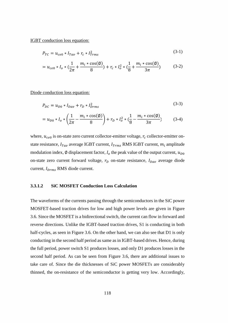
118

IGBT conduction loss equation:

𝑃𝑇𝐶 = 𝑢𝑐𝑒0 ∗ 𝐼𝑇𝑎𝑣 + 𝑟𝑐 ∗ 𝐼𝑇𝑟𝑚𝑠

2 (3-1)

= 𝑢𝑐𝑒0 ∗ 𝐼𝑜 ∗ (

1

2𝜋+𝑚𝑖 ∗ cos(∅)

8) + 𝑟𝑐 ∗ 𝐼𝑜

2 ∗ (1

8+𝑚𝑖 ∗ cos (∅)

3𝜋) (3-2)

Diode conduction loss equation:

𝑃𝐷𝐶 = 𝑢𝐷0 ∗ 𝐼𝐷𝑎𝑣 + 𝑟𝐷 ∗ 𝐼𝐷𝑟𝑚𝑠

2 (3-3)

= 𝑢𝐷0 ∗ 𝐼𝑜 ∗ (

1

2𝜋−𝑚𝑖 ∗ cos(∅)

8) + 𝑟𝐷 ∗ 𝐼𝑜

2 ∗ (1

8−𝑚𝑖 ∗ cos(∅)

3𝜋) (3-4)

where, 𝑢𝑐𝑒0 is on-state zero current collector-emitter voltage, 𝑟𝑐 collector-emitter on-

state resistance, 𝐼𝑇𝑎𝑣 average IGBT current, 𝐼𝑇𝑟𝑚𝑠 RMS IGBT current, 𝑚𝑖 amplitude

modulation index, ∅ displacement factor, 𝐼𝑜 the peak value of the output current, 𝑢𝐷0

on-state zero current forward voltage, 𝑟𝐷 on-state resistance, 𝐼𝐷𝑎𝑣 average diode

current, 𝐼𝐷𝑟𝑚𝑠 RMS diode current.

3.3.1.2 SiC MOSFET Conduction Loss Calculation

The waveforms of the currents passing through the semiconductors in the SiC power

MOSFET-based traction drives for low and high power levels are given in Figure

3.6. Since the MOSFET is a bidirectional switch, the current can flow in forward and

reverse directions. Unlike the IGBT-based traction drives, S1 is conducting in both

half-cycles, as seen in Figure 3.6. On the other hand, we can also see that D1 is only

conducting in the second half period as same as in IGBT-based drives. Hence, during

the full period, power switch S1 produces losses, and only D1 produces losses in the

second half period. As can be seen from Figure 3.6, there are additional issues to

take care of. Since the die thicknesses of SiC power MOSFETs are considerably

thinned, the on-resistance of the semiconductor is getting very low. Accordingly,

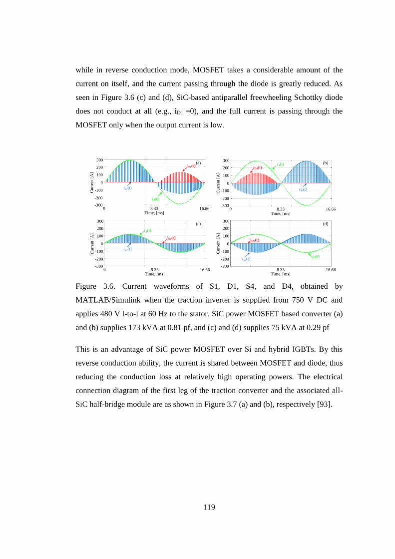
119

while in reverse conduction mode, MOSFET takes a considerable amount of the

current on itself, and the current passing through the diode is greatly reduced. As

seen in Figure 3.6 (c) and (d), SiC-based antiparallel freewheeling Schottky diode

does not conduct at all (e.g., iD1 =0), and the full current is passing through the

MOSFET only when the output current is low.

Cu

rrent

[A]

0

100

200

iA(t)

16.66Time, [ms]

iS1(t)

iD1(t)

300

-100

-200

-3008.330

Cu

rrent

[A]

0

100

200iA(t)

16.66Time, [ms]

iS4(t)

iD4(t)

300

-100

-200

-3008.330

Cu

rrent

[A]

0

100

200

iA(t)

16.66Time, [ms]

iS4(t)

iD4(t)

300

-100

-200

-3008.33

Cu

rrent

[A]

0

100

200

16.66Time, [ms]

iS1(t)

iD1(t)

300

-100

-200

-3008.330

iA(t)

(a) (b)

(c) (d)

Figure 3.6. Current waveforms of S1, D1, S4, and D4, obtained by


applies 480 V l-to-l at 60 Hz to the stator. SiC power MOSFET based converter (a)

and (b) supplies 173 kVA at 0.81 pf, and (c) and (d) supplies 75 kVA at 0.29 pf

This is an advantage of SiC power MOSFET over Si and hybrid IGBTs. By this

reverse conduction ability, the current is shared between MOSFET and diode, thus

reducing the conduction loss at relatively high operating powers. The electrical

connection diagram of the first leg of the traction converter and the associated all-

SiC half-bridge module are as shown in Figure 3.7 (a) and (b), respectively [93].

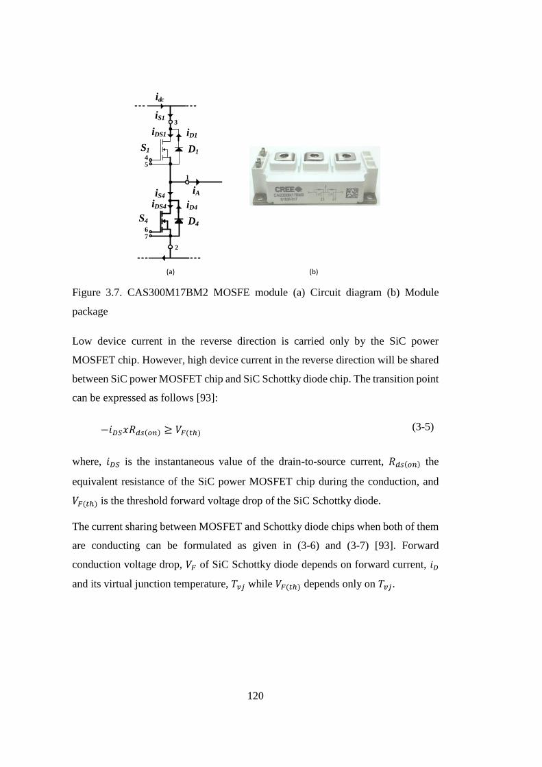
120

S1 D1

iA

idc

iS1

iDS1 iD1

S4 D4

iS4

iDS4 iD4

4

1

5

3

2

67

(a) (b)

Figure 3.7. CAS300M17BM2 MOSFE module (a) Circuit diagram (b) Module

package

Low device current in the reverse direction is carried only by the SiC power

MOSFET chip. However, high device current in the reverse direction will be shared

between SiC power MOSFET chip and SiC Schottky diode chip. The transition point

can be expressed as follows [93]:

−𝑖𝐷𝑆𝑥𝑅𝑑𝑠(𝑜𝑛) ≥ 𝑉𝐹(𝑡ℎ) (3-5)

where, 𝑖𝐷𝑆 is the instantaneous value of the drain-to-source current, 𝑅𝑑𝑠(𝑜𝑛) the

equivalent resistance of the SiC power MOSFET chip during the conduction, and

𝑉𝐹(𝑡ℎ) is the threshold forward voltage drop of the SiC Schottky diode.

The current sharing between MOSFET and Schottky diode chips when both of them

are conducting can be formulated as given in (3-6) and (3-7) [93]. Forward

conduction voltage drop, 𝑉𝐹 of SiC Schottky diode depends on forward current, 𝑖𝐷

and its virtual junction temperature, 𝑇𝑣𝑗 while 𝑉𝐹(𝑡ℎ) depends only on 𝑇𝑣𝑗.

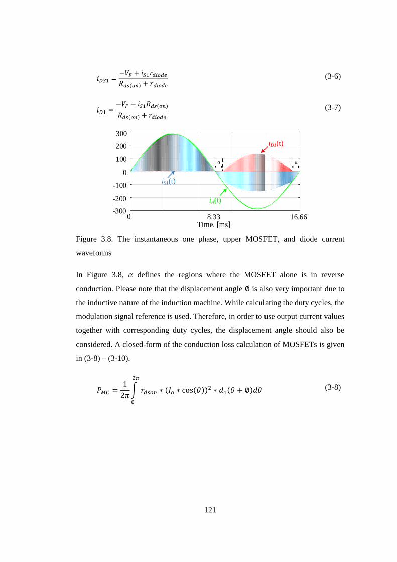
121

𝑖𝐷𝑆1 =

−𝑉𝐹 + 𝑖𝑆1𝑟𝑑𝑖𝑜𝑑𝑒𝑅𝑑𝑠(𝑜𝑛) + 𝑟𝑑𝑖𝑜𝑑𝑒

(3-6)

𝑖𝐷1 =

−𝑉𝐹 − 𝑖𝑆1𝑅𝑑𝑠(𝑜𝑛)

𝑅𝑑𝑠(𝑜𝑛) + 𝑟𝑑𝑖𝑜𝑑𝑒 (3-7)

0

100

200

iA(t)

16.66Time, [ms]

iS1(t)

iD1(t)

300

-100

-200

-3008.330

α α

Figure 3.8. The instantaneous one phase, upper MOSFET, and diode current

waveforms

In Figure 3.8, 𝛼 defines the regions where the MOSFET alone is in reverse

conduction. Please note that the displacement angle ∅ is also very important due to

the inductive nature of the induction machine. While calculating the duty cycles, the

modulation signal reference is used. Therefore, in order to use output current values

together with corresponding duty cycles, the displacement angle should also be

considered. A closed-form of the conduction loss calculation of MOSFETs is given

in (3-8) – (3-10).

𝑃𝑀𝐶 =1

2𝜋∫ 𝑟𝑑𝑠𝑜𝑛 ∗ (𝐼𝑜 ∗ cos(𝜃))

2 ∗ 𝑑1(𝜃 + ∅)𝑑𝜃

2𝜋

0

(3-8)

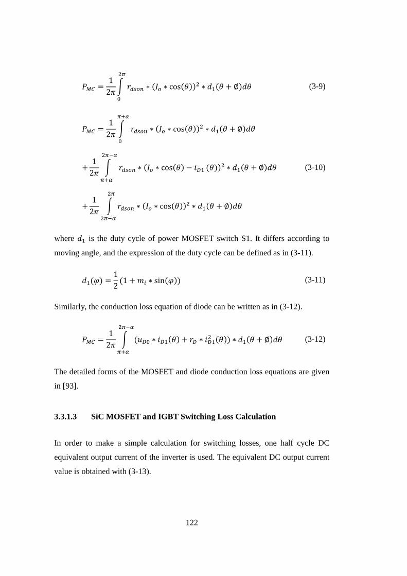
122

𝑃𝑀𝐶 =1


2 ∗ 𝑑1(𝜃 + ∅)𝑑𝜃

2𝜋

0

(3-9)

𝑃𝑀𝐶 =1


2 ∗ 𝑑1(𝜃 + ∅)𝑑𝜃

𝜋+𝛼

0

+1

2𝜋∫ 𝑟𝑑𝑠𝑜𝑛 ∗ (𝐼𝑜 ∗ cos(𝜃) − 𝑖𝐷1 (𝜃))

2 ∗ 𝑑1(𝜃 + ∅)𝑑𝜃

2𝜋−𝛼

𝜋+𝛼

+1


2 ∗ 𝑑1(𝜃 + ∅)𝑑𝜃

2𝜋

2𝜋−𝛼

(3-10)

where 𝑑1 is the duty cycle of power MOSFET switch S1. It differs according to

moving angle, and the expression of the duty cycle can be defined as in (3-11).

𝑑1(𝜑) =

1

2(1 + 𝑚𝑖 ∗ sin(𝜑)) (3-11)

Similarly, the conduction loss equation of diode can be written as in (3-12).

𝑃𝑀𝐶 =1

2𝜋∫ (𝑢𝐷0 ∗ 𝑖𝐷1(𝜃) + 𝑟𝐷 ∗ 𝑖𝐷1

2 (𝜃)

2𝜋−𝛼

𝜋+𝛼

) ∗ 𝑑1(𝜃 + ∅)𝑑𝜃 (3-12)

The detailed forms of the MOSFET and diode conduction loss equations are given

in [93].

3.3.1.3 SiC MOSFET and IGBT Switching Loss Calculation

In order to make a simple calculation for switching losses, one half cycle DC

equivalent output current of the inverter is used. The equivalent DC output current

value is obtained with (3-13).

123

𝐼𝐷𝐶 =

1

𝜋∗ 𝐼𝑜 (3-13)

By using 𝐼𝐷𝐶, 𝐸𝑜𝑛 and 𝐸𝑜𝑓𝑓 energies of MOSFET, IGBT, and diode can be found

from the product datasheets.

IGBT and MOSFET switching loss equation:

𝑃𝑇𝑠𝑤 = (𝐸𝑇𝑜𝑛 + 𝐸𝑇𝑜𝑓𝑓) ∗ 𝑓𝑠𝑤 ∗

𝐼𝑜𝜋𝐼𝑁

∗𝑉𝐷𝐶−𝑙𝑖𝑛𝑘𝑉𝑁

(3-14)

𝑃𝑀𝑠𝑤 = (𝐸𝑀𝑜𝑛 + 𝐸𝑀𝑜𝑓𝑓) ∗ 𝑓𝑠𝑤 ∗



(3-15)

Diode switching loss equation:

𝑃𝐷𝑠𝑤 = (𝐸𝐷𝑜𝑛 + 𝐸𝐷𝑜𝑓𝑓) ∗ 𝑓𝑠𝑤 ∗



(3-16)

Total losses of IGBT, MOSFET, and diode can be finally obtained with the following

equations:

𝑃𝑇𝑡𝑜𝑡𝑎𝑙 = 𝑃𝑇𝐶 + 𝑃𝑇𝑠𝑤 (3-17)

𝑃𝐷𝑡𝑜𝑡𝑎𝑙 = 𝑃𝐷𝐶 + 𝑃𝐷𝑠𝑤 (3-18)

Simulation software of IPOSIM, Melcosim, Fuji IGBT Simulator, and SpeedFit are

used in performance calculations respectively of FF300R17KE4P, CM300DY-34T,

2MSI400VAE-170-53, and CAS300M17BM2 for different switching frequencies.

Note that the traction application compliant semiconductors were not used in this

study to find the comparable package, current, and voltage specifications that are

similar to the SiC MOSFET module. The power loss analysis results of the 2L

inverter are summarized in Table 3.6. The allowable junction temperature limit is

taken as 120°C for calculations in order to increase the lifetime of the power

semiconductor. In the previous section, 8 kHz is determined as the minimum

switching frequency to satisfy the peak-to-peak toque ripple requirement.

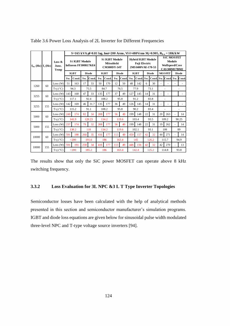
124

Table 3.6 Power Loss Analysis of 2L Inverter for Different Frequencies

The results show that only the SiC power MOSFET can operate above 8 kHz

switching frequency.

3.3.2 Loss Evaluation for 3L NPC &3 L T Type Inverter Topologies

Semiconductor losses have been calculated with the help of analytical methods

presented in this section and semiconductor manufacturer’s simulation programs.

IGBT and diode loss equations are given below for sinusoidal pulse width modulated

three-level NPC and T-type voltage source inverters [94].

Sw. Cond. Sw. Cond. Sw. Cond. Sw. Cond. Sw. Cond. Sw. Cond. Sw. Cond. Sw. Cond.

Loss (W) 51 163 17 33 50 170 12 50 48 142 6 30 - - - -

Tvj (°C)

Loss (W) 143 168 47 33 135 177 37 49 127 145 14 31 - - -

Tvj (°C)

Loss (W) 142 169 46 31.7 135 177 36 49 126 145 14 31 - - - -

Tvj (°C)

Loss (W) 240 174 82 34 208 177 56 49 199 148 22 31 20 263 - 14

Tvj (°C)

Loss (W) 237 174 79 32 208 177 56 49 199 148 22 31 19 262 - 14

Tvj (°C)

Loss (W) 591 190 260 35 416 177 113 49 450 157 42 32 44 271 - 14

Tvj (°C)

Loss (W) 591 191 258 34 416 177 113 49 446 156 42 32 42 270 - 13

Tvj (°C)

Loss &

Junc.

Temp

fs (Hz)fSw (Hz)

10000 155>200 185.2 186

Hybrid IGBT Module

Fuji Electric

2MSI400VAE-170-53

Si IGBT Module

Mitsubishi

CM300DY-34T

Si IGBT Module

Infineon FF300R17KE4

115.7163.4 145 126.210000 60

>200 191.6 186

119.6 102.1 93.1

114.8 93.8

94.9

163.4 142.4 125.2

108 895000 155

138.2 118 134.2

119.6 103.4 93.5 109.2 90.255000 60

141.9 120.23 134.2

95.8 90.2 83.4 - -3255 155

115.2 91.1 108.2

95.8 91.2 83.8 -3255 60

117.1 92.4 108.2

76.5 77.9 73.1 - -1260 60

94.3 75.5 84.7

S=165 kVA pf=0.81 lag, Iout=200 Arms, Vl-l=480Vrms Mi=0.905, Rh-a = 18K/kW

SiC MOSFET

Module

Wolfspeed/Cree

CAS300M17BM2

IGBT Diode IGBT Diode IGBT Diode MO SFET Diode

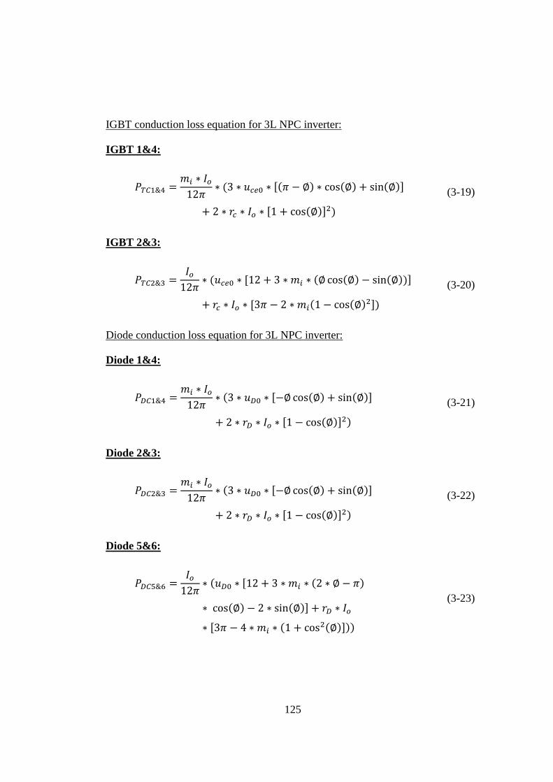
125

IGBT conduction loss equation for 3L NPC inverter:

IGBT 1&4:

𝑃𝑇𝐶1&4 =𝑚𝑖 ∗ 𝐼𝑜12𝜋

∗ (3 ∗ 𝑢𝑐𝑒0 ∗ [(𝜋 − ∅) ∗ cos(∅) + sin(∅)]

+ 2 ∗ 𝑟𝑐 ∗ 𝐼𝑜 ∗ [1 + cos(∅)]2)

(3-19)

IGBT 2&3:

𝑃𝑇𝐶2&3 =𝐼𝑜12𝜋

∗ (𝑢𝑐𝑒0 ∗ [12 + 3 ∗ 𝑚𝑖 ∗ (∅ cos(∅) − sin(∅))]

+ 𝑟𝑐 ∗ 𝐼𝑜 ∗ [3𝜋 − 2 ∗ 𝑚𝑖(1 − cos(∅)2])

(3-20)

Diode conduction loss equation for 3L NPC inverter:

Diode 1&4:

𝑃𝐷𝐶1&4 =𝑚𝑖 ∗ 𝐼𝑜12𝜋

∗ (3 ∗ 𝑢𝐷0 ∗ [−∅ cos(∅) + sin(∅)]

+ 2 ∗ 𝑟𝐷 ∗ 𝐼𝑜 ∗ [1 − cos(∅)]2)

(3-21)

Diode 2&3:


∗ (3 ∗ 𝑢𝐷0 ∗ [−∅ cos(∅) + sin(∅)]

+ 2 ∗ 𝑟𝐷 ∗ 𝐼𝑜 ∗ [1 − cos(∅)]2)

(3-22)

Diode 5&6:

𝑃𝐷𝐶5&6 =𝐼𝑜12𝜋

∗ (𝑢𝐷0 ∗ [12 + 3 ∗ 𝑚𝑖 ∗ (2 ∗ ∅ − 𝜋)

∗ cos(∅) − 2 ∗ sin(∅)] + 𝑟𝐷 ∗ 𝐼𝑜

∗ [3𝜋 − 4 ∗ 𝑚𝑖 ∗ (1 + cos2(∅)]))

(3-23)

126

IGBT switching loss equation for 3L NPC inverter:

IGBT 1&4:

𝑃𝑇1&4𝑆𝑊 = (𝐸𝑇𝑜𝑛(𝑁) + 𝐸𝑇𝑜𝑓𝑓(𝑁)) ∗ 𝑓𝑠𝑤 ∗𝐼𝑜𝐼𝑁∗(0.5 ∗ 𝑉𝐷𝐶−𝑙𝑖𝑛𝑘)

𝑉𝑁

∗ (1

2𝜋∗ [1 + cos(∅)])

(3-24)

IGBT 2&3:


𝑉𝑁

∗ (1

2𝜋∗ [1 − cos(∅)])

(3-25)

Diode 1&2:

𝑃𝐷1&2𝑠𝑤 = 𝐸𝑅𝐸𝐶(𝑁) ∗ 𝑓𝑠𝑤 ∗𝐼𝑜𝐼𝑁∗(0.5 ∗ 𝑉𝐷𝐶−𝑙𝑖𝑛𝑘)

𝑉𝑁

∗ (1

2𝜋∗ [1 − cos(∅)])

(3-26)

Diode 2&3:

𝑃𝐷2&3𝑠𝑤 = 0 (3-27)

Diode 5&6:


𝑉𝑁

∗ (1

2𝜋∗ [1 + cos(∅)])

(3-28)

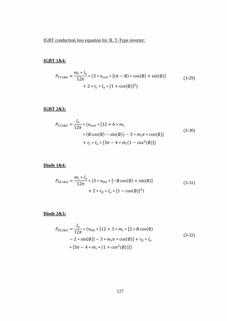
127

IGBT conduction loss equation for 3L T-Type inverter:

IGBT 1&4:

𝑃𝑇𝐶1&4 =𝑚𝑖 ∗ 𝐼𝑜12𝜋

∗ (3 ∗ 𝑢𝑐𝑒0 ∗ [(𝜋 − ∅) ∗ cos(∅) + sin(∅)]

+ 2 ∗ 𝑟𝑐 ∗ 𝐼𝑜 ∗ [1 + cos(∅)]2)

(3-29)

IGBT 2&3:

𝑃𝑇𝐶2&3 =𝐼𝑜12𝜋

∗ (𝑢𝑐𝑒0 ∗ [12 + 6 ∗ 𝑚𝑖

∗ (∅ cos(∅) − sin(∅)) − 3 ∗ 𝑚𝑖𝜋 ∗ cos (∅)]

+ 𝑟𝑐 ∗ 𝐼𝑜 ∗ [3𝜋 − 4 ∗ 𝑚𝑖(1 − cos2(∅)])

(3-30)

Diode 1&4:


∗ (3 ∗ 𝑢𝐷0 ∗ [−∅ cos(∅) + sin(∅)]

+ 2 ∗ 𝑟𝐷 ∗ 𝐼𝑜 ∗ [1 − cos(∅)]2)

(3-31)

Diode 2&3:

𝑃𝐷𝐶2&3 =𝐼𝑜12𝜋

∗ (𝑢𝐷0 ∗ [12 + 3 ∗ 𝑚𝑖 ∗ [2 ∗ ∅ cos(∅)

− 2 ∗ sin(∅)] − 3 ∗ 𝑚𝑖𝜋 ∗ cos(∅)] + 𝑟𝐷 ∗ 𝐼𝑜

∗ [3𝜋 − 4 ∗ 𝑚𝑖 ∗ (1 + cos2(∅))])

(3-32)

128

IGBT switching loss equation for 3L T-type inverter:

IGBT 1&4:

𝑃𝑇1&4𝑆𝑊 = (𝐸𝑇𝑜𝑛(𝑁) + 𝐸𝑇𝑜𝑓𝑓(𝑁)) ∗ 𝑓𝑠𝑤 ∗𝐼𝑜𝐼𝑁∗𝑉𝐷𝐶−𝑙𝑖𝑛𝑘𝑉𝑁(𝑇1&4)

∗ (1

2𝜋∗ [1 + cos(∅)])

(3-33)

IGBT 2&3:


𝑉𝑁(𝑇2&3)

∗ (1

2𝜋∗ [1 − cos(∅)])

(3-34)

Diode 1&4:

𝑃𝐷1&2𝑠𝑤 = 𝐸𝑅𝐸𝐶(𝑁) ∗ 𝑓𝑠𝑤 ∗𝐼𝑜𝐼𝑁∗𝑉𝐷𝐶−𝑙𝑖𝑛𝑘𝑉𝑁(𝐷1&4)

∗ (1

2𝜋∗ [1 − cos(∅)])

(3-35)

Diode 2&3:


𝑉𝑁(𝐷2&3)

∗ (1

2𝜋∗ [1 + cos(∅)])

(3-36)

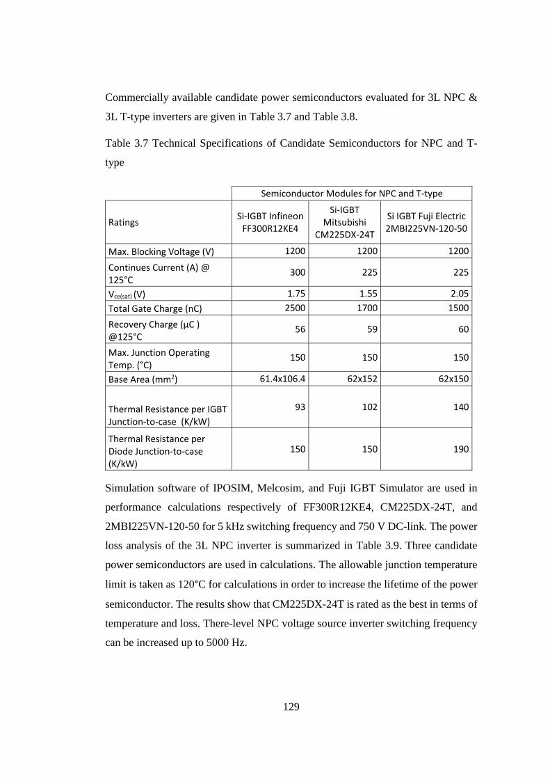
129

Commercially available candidate power semiconductors evaluated for 3L NPC &

3L T-type inverters are given in Table 3.7 and Table 3.8.

Table 3.7 Technical Specifications of Candidate Semiconductors for NPC and T-

type

Semiconductor Modules for NPC and T-type

Ratings Si-IGBT Infineon

FF300R12KE4

Si-IGBT Mitsubishi

CM225DX-24T

Si IGBT Fuji Electric 2MBI225VN-120-50

Max. Blocking Voltage (V) 1200 1200 1200

Continues Current (A) @ 125°C

300 225 225

Vce(sat) (V) 1.75 1.55 2.05

Total Gate Charge (nC) 2500 1700 1500

Recovery Charge (µC ) @125°C

56 59 60

Max. Junction Operating Temp. (°C)

150 150 150

Base Area (mm2) 61.4x106.4 62x152 62x150

Thermal Resistance per IGBT Junction-to-case (K/kW)

93 102 140

Thermal Resistance per Diode Junction-to-case (K/kW)

150 150 190

Simulation software of IPOSIM, Melcosim, and Fuji IGBT Simulator are used in

performance calculations respectively of FF300R12KE4, CM225DX-24T, and

2MBI225VN-120-50 for 5 kHz switching frequency and 750 V DC-link. The power

loss analysis of the 3L NPC inverter is summarized in Table 3.9. Three candidate

power semiconductors are used in calculations. The allowable junction temperature

limit is taken as 120°C for calculations in order to increase the lifetime of the power

semiconductor. The results show that CM225DX-24T is rated as the best in terms of

temperature and loss. There-level NPC voltage source inverter switching frequency

can be increased up to 5000 Hz.

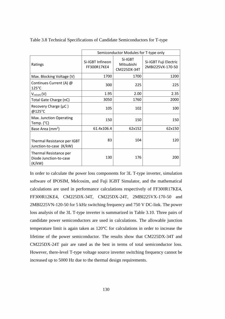
130

Table 3.8 Technical Specifications of Candidate Semiconductors for T-type

Semiconductor Modules for T-type only

Ratings Si-IGBT Infineon

FF300R17KE4

Si-IGBT Mitsubishi

CM225DX-34T

Si-IGBT Fuji Electric 2MBI225VX-170-50

Max. Blocking Voltage (V) 1700 1700 1200

Continues Current (A) @ 125°C

300 225 225

Vce(sat) (V) 1.95 2.00 2.35

Total Gate Charge (nC) 3050 1760 2000

Recovery Charge (µC ) @125°C

105 102 100

Max. Junction Operating Temp. (°C)

150 150 150

Base Area (mm2) 61.4x106.4 62x152 62x150

Thermal Resistance per IGBT Junction-to-case (K/kW)

83 104 120

Thermal Resistance per Diode Junction-to-case (K/kW)

130 176 200

In order to calculate the power loss components for 3L T-type inverter, simulation

software of IPOSIM, Melcosim, and Fuji IGBT Simulator, and the mathematical

calculations are used in performance calculations respectively of FF300R17KE4,

FF300R12KE4, CM225DX-34T, CM225DX-24T, 2MBI225VX-170-50 and

2MBI225VN-120-50 for 5 kHz switching frequency and 750 V DC-link. The power

loss analysis of the 3L T-type inverter is summarized in Table 3.10. Three pairs of

candidate power semiconductors are used in calculations. The allowable junction

temperature limit is again taken as 120°C for calculations in order to increase the

lifetime of the power semiconductor. The results show that CM225DX-34T and

CM225DX-24T pair are rated as the best in terms of total semiconductor loss.

However, there-level T-type voltage source inverter switching frequency cannot be

increased up to 5000 Hz due to the thermal design requirements.

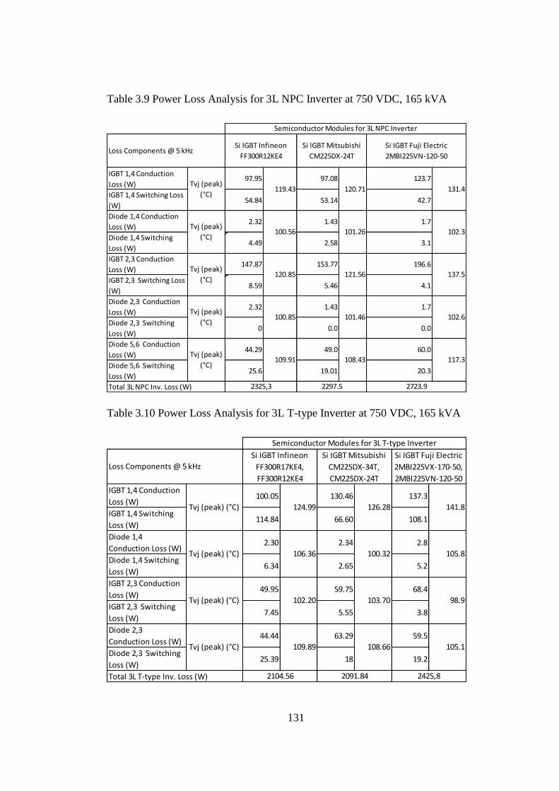
131

Table 3.9 Power Loss Analysis for 3L NPC Inverter at 750 VDC, 165 kVA

Table 3.10 Power Loss Analysis for 3L T-type Inverter at 750 VDC, 165 kVA

IGBT 1,4 Conduction

Loss (W)97.95 97.08 123.7

IGBT 1,4 Switching Loss

(W)54.84 53.14 42.7

Diode 1,4 Conduction

Loss (W)2.32 1.43 1.7

Diode 1,4 Switching

Loss (W)4.49 2.58 3.1

IGBT 2,3 Conduction

Loss (W)147.87 153.77 196.6

IGBT 2,3 Switching Loss

(W)8.59 5.46 4.1


Loss (W)2.32 1.43 1.7

Diode 2,3 Switching

Loss (W)0 0.0 0.0


Loss (W)44.29 49.0 60.0

Diode 5,6 Switching

Loss (W)25.6 19.01 20.3

2297.5 2723.9

119.43

100.56

120.85

100.85

109.91

2325,3Total 3L NPC Inv. Loss (W)

Si IGBT Fuji Electric

2MBI225VN-120-50

Si IGBT Mitsubishi

CM225DX-24T

Si IGBT Infineon

FF300R12KE4

Semiconductor Modules for 3L NPC Inverter

120.71

101.26

121.56

101.46

108.43

Tvj (peak)

(°C)

Tvj (peak)

(°C)

Tvj (peak)

(°C)

Tvj (peak)

(°C)

Tvj (peak)

(°C)

131.4

102.3

137.5

102.6

117.3

Loss Components @ 5 kHz

IGBT 1,4 Conduction

Loss (W)100.05 130.46 137.3

IGBT 1,4 Switching

Loss (W)114.84 66.60 108.1

Diode 1,4

Conduction Loss (W)2.30 2.34 2.8

Diode 1,4 Switching

Loss (W)6.34 2.65 5.2

IGBT 2,3 Conduction

Loss (W)49.95 59.75 68.4

IGBT 2,3 Switching

Loss (W)7.45 5.55 3.8

Diode 2,3

Conduction Loss (W)44.44 63.29 59.5

Diode 2,3 Switching

Loss (W)25.39 18 19.2

100.32 105.8Tvj (peak) (°C) 106.36

Semiconductor Modules for 3L T-type Inverter

Loss Components @ 5 kHz

Si IGBT Infineon

FF300R17KE4,

FF300R12KE4

Si IGBT Mitsubishi

CM225DX-34T,

CM225DX-24T

Si IGBT Fuji Electric

2MBI225VX-170-50,

2MBI225VN-120-50

Tvj (peak) (°C) 124.99 126.28 141.8

Total 3L T-type Inv. Loss (W) 2104.56 2091.84 2425,8

Tvj (peak) (°C) 102.20 103.70 98.9

Tvj (peak) (°C) 109.89 108.66 105.1

132

3.4 Overall System Efficiency

In this thesis, the efficiency of the traction motor drive is maximized by switching

the traction inverter at the optimum frequency. Also, the operating range of the

virtual junction temperature of the SiC power MOSFET is affected by the switching

frequency. Lower junction temperatures lead to significantly longer lifetimes for

power semiconductors. The overall efficiency of the traction motor drive is the

multiplication of traction inverter efficiency and motor efficiency. The main power

loss components are conduction and switching losses for the inverter and copper and

core loss for the traction motor. These power loss components are determined by

tests as well as some detailed simulations. To determine the power loss components

of the traction motor, it is driven by the loading machine at synchronous speed

(nr=1800 rpm) corresponding to the rated frequency (fs=60 Hz), the rated voltage is

applied (Vs=480 V l-to-l), and the stator line current and stator power input are

measured as a function of the inverter switching frequency. Core loss is separated

from stator copper loss using the stator resistance provided by the motor

manufacturer as a function of the drive switching frequency and stator temperature,

and line currents. Core loss includes hysteresis loss, eddy current loss, and other

mechanical loss components. The hysteresis losses increase with an increase in AC

flux density, 𝐵𝐴𝐶 and operating and switching frequency. The general form of the

hysteresis and eddy current loss equations are given in (3-37) and (3-38).

𝑃ℎ𝑦𝑠 = 𝑘𝑓𝛼(𝐵𝐴𝐶)𝛽 (3-37)

where k, 𝛼, and are constants that depend on the core material. 𝐵𝐴𝐶 contains two

components: i) Low-frequency component @ motor stator fundamental frequency

ii) High-frequency component @ switching frequency. The high-frequency

components are decreased a considerable amount with the increased switching

frequency.

𝑃𝑒𝑑𝑑𝑦 =𝑑2𝑤2𝐵2

24𝜌𝑐𝑜𝑟𝑒 (3-38)

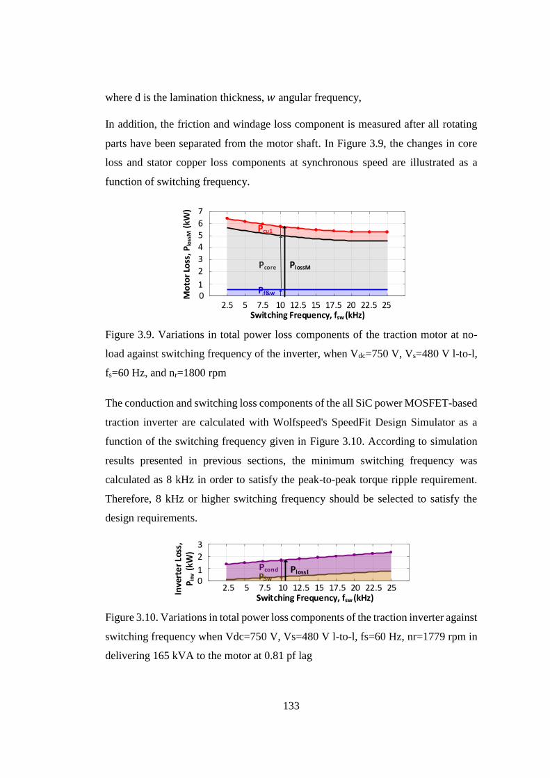
133

where d is the lamination thickness, 𝑤 angular frequency,

In addition, the friction and windage loss component is measured after all rotating

parts have been separated from the motor shaft. In Figure 3.9, the changes in core

loss and stator copper loss components at synchronous speed are illustrated as a

function of switching frequency.

Switching Frequency, fsw (kHz)

Pf&w

Pcore

Pcu1

PlossM

2.5 5 7.5 10 12.5 15 17.5 22.520 25

Mo

tor

Loss

, Plo

ssM

(kW

) 7

654

3

2

10

Figure 3.9. Variations in total power loss components of the traction motor at no-

load against switching frequency of the inverter, when Vdc=750 V, Vs=480 V l-to-l,

fs=60 Hz, and nr=1800 rpm

The conduction and switching loss components of the all SiC power MOSFET-based

traction inverter are calculated with Wolfspeed's SpeedFit Design Simulator as a

function of the switching frequency given in Figure 3.10. According to simulation

results presented in previous sections, the minimum switching frequency was

calculated as 8 kHz in order to satisfy the peak-to-peak torque ripple requirement.

Therefore, 8 kHz or higher switching frequency should be selected to satisfy the

design requirements.

2.5 5 7.5 10 12.5 15 17.5 22.520 25Switching Frequency, fsw (kHz)

Inve

rte

r Lo

ss,

Pin

v (k

W)

3

2

10 PSw

Pcond PlossI

Figure 3.10. Variations in total power loss components of the traction inverter against

switching frequency when Vdc=750 V, Vs=480 V l-to-l, fs=60 Hz, nr=1779 rpm in

delivering 165 kVA to the motor at 0.81 pf lag

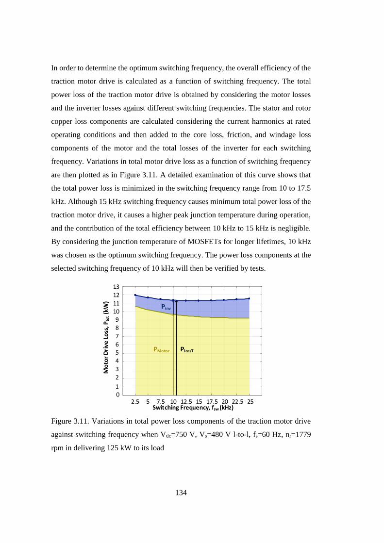
134

In order to determine the optimum switching frequency, the overall efficiency of the

traction motor drive is calculated as a function of switching frequency. The total

power loss of the traction motor drive is obtained by considering the motor losses

and the inverter losses against different switching frequencies. The stator and rotor

copper loss components are calculated considering the current harmonics at rated

operating conditions and then added to the core loss, friction, and windage loss

components of the motor and the total losses of the inverter for each switching

frequency. Variations in total motor drive loss as a function of switching frequency

are then plotted as in Figure 3.11. A detailed examination of this curve shows that

the total power loss is minimized in the switching frequency range from 10 to 17.5

kHz. Although 15 kHz switching frequency causes minimum total power loss of the

traction motor drive, it causes a higher peak junction temperature during operation,

and the contribution of the total efficiency between 10 kHz to 15 kHz is negligible.

By considering the junction temperature of MOSFETs for longer lifetimes, 10 kHz

was chosen as the optimum switching frequency. The power loss components at the

selected switching frequency of 10 kHz will then be verified by tests.

PMotor

Pinv

PlossT

8

7

654

3

2

10

2.5 5 7.5 10 12.5 15 17.5 22.520 25

Mo

tor

Dri

ve L

oss

, Pto

t (k

W)

13

12

11109

Switching Frequency, fsw (kHz)

Figure 3.11. Variations in total power loss components of the traction motor drive

against switching frequency when Vdc=750 V, Vs=480 V l-to-l, fs=60 Hz, nr=1779

rpm in delivering 125 kW to its load

135

3.4.1 Loss Comparison of Two-Level & Three-Level Converter

Topologies

Improvement of output waveform quality and output power increase are the

advantages well-known advantages of multilevel converters. Improvements in

output waveform quality were already explained in Chapter 2, and later it will be

examined in detail in Chapter 4. In this section, the loss, cost, volume, and reliability

comparisons are briefly examined.

The power loss analysis shows that Si-IGBT-based two-level inverter topology can

survive at switching frequencies around 3.5 kHz at most. Above this switching

frequency, the junction temperatures rise above 120 °C with full Si-IGBT-based

solutions. Thus, full Si-based IGBT modules do not satisfy the design requirements.

Together with Si-IGBT modules, a hybrid IGBT module and full SiC MOSFET

module are also taken into account in power loss calculations. The analysis results

show that even if the hybrid IGBT module lets to increase switching frequency

considerable amount, it does not still satisfy the design requirements. Only the full

SiC MOSFET-based two-level solution has shown great success in satisfying the

requirements with two-level inverter topology. On the other hand, Si-IGBT-based

three-level T-type and NPC inverter topologies also provide great advantages to meet

design requirements. The summary of power loss analysis, the unit cost of power

electronic blocks, and the total semiconductor areas are given in Table 3.11. In order

to make a fair comparison, the effective switching frequencies are also set to 10 kHz

(i.e., 5 kHz switching frequency) for three-level converters. In Table 3.11, only

products showing the best performance results are listed.

136

Table 3.11 Comparison of Different Inverter Topologies In Terms of Losses, Unit

Costs and Semiconductor Base Areas

Although the same total power losses are obtained with the SiC MOSFET-based

two-level inverter solution and Si-IGBT-based three-level T-type topology, the

maximum junction temperature target is not satisfied with T-type topology. On the

other hand, among the converter topologies, three-level NPC topology has the

highest total power loss. If we compare the topologies in terms of power block costs,

the T-type inverter offers the cheapest solution. The power block costs contain

laminated busbars, heatsink, gate-driver, semiconductor, DC-link capacitor, phase

current sensor, and cable prices. However, the difference between power block costs

is too small to be considered in the total converter cost. It is seen that the biggest

difference between the converter topologies is the semiconductor area. Hence, it can

be said that the smallest and the most efficient topology that meets the requirements

is the SiC MOSFET-based two-level inverter. Moreover, another issue that needs to

be compared is reliability. The two-level solution is also very advantageous in terms

of reliability due to the low number of components and the ability to withstand higher

thermal stresses. If we make an additional comparison between the three-level

converter topologies, it is seen that the T-type topology, where the number of serial

switches is less, is more advantageous at low voltage and power levels and relatively

low-frequency applications. The three-level NPC inverter is superior for relatively

high switching frequencies.

Total Switch Loss

(W)1767.00 1574.16 1856.7

Total Diode Loss

(W)324.00 517.68 440.8

Topologies

Loss Components

SiC MOSFET based Two-

level Inverter @ fsw = 10

kHz CAS300M17BM2

Si IGBT based Three-level T-

Type Inverter @ fsw = 5 kHz

CM225DX-34T&CM225DX-24T

Si IGBT based Three-level

NPC Inverter @ fsw = 5 kHz

CM225DX-24T

Tvj

(peak)

(°C)

120.2 126.28 121.56

Total Power Loss (W) 2297.5

1.048

4.33Semiconductor Area (Unit)

2091.00

1.024

1

2091.84

1.000

2.89

Cost for Power Electronic

Block (Unit)

137

3.5 Selection of Input Filter Components

Most of the railway DC electrification systems consist of six or twelve pulse bridge

rectifiers, as mentioned in Chapter 1. These rectifiers inject low-frequency voltage

ripple on the third rail or catenary line. Besides this, high-frequency harmonics are

imposed on the third rail or catenary line due to the switching behavior of the traction

inverter. In addition to this, the third rail or catenary voltage can be interrupted or

discontinuous in normal operation due to some physical difficulties. This can cause

voltage spikes due to the sudden change of highly demanded current and parasitic

inductances of the power lines. This can end up with semiconductor failure.

Moreover, voltage dips can also be seen at the electrification line due to some

electrical and mechanical failures. This situation can also cause huge current flow

from traction inverter DC-link capacitors to electrification lines. In order to eliminate

all these problems, an LC filter with a low cut-off frequency is needed at the input

stage of the traction inverter. In these applications, the cut-off frequency is selected

below the grid frequency [24].

Following criteria should be taken into account for the selection of input filter

components;

The DC-link capacitance should be enough to reach the target voltage ripple,

The DC-link capacitor should have enough RMS current carrying capacity,

The laminated busbar structure with DC-link capacitor should provide

sufficiently low parasitic inductance and resistance to filter out high-

frequency harmonics and prevent switching spikes,

The cut-off frequency of the input filter should be appropriate for harmonics

produced from six and twelve pulse rectifiers,

The line reactor should have sufficiently high inductance to limit current

under failure instant (i.e., short circuit failures),

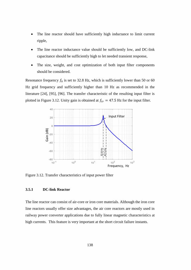
138

The line reactor should have sufficiently high inductance to limit current

ripple,

The line reactor inductance value should be sufficiently low, and DC-link

capacitance should be sufficiently high to let needed transient response,

The size, weight, and cost optimization of both input filter components

should be considered.

Resonance frequency 𝑓0 is set to 32.8 Hz, which is sufficiently lower than 50 or 60

Hz grid frequency and sufficiently higher than 10 Hz as recommended in the

literature [24], [95], [96]. The transfer characteristic of the resulting input filter is

plotted in Figure 3.12. Unity gain is obtained at 𝑓𝑡𝑟 = 47.5 Hz for the input filter.

Input Filter

32

.8 H

z

47

.5 H

z

Frequency, Hz

Figure 3.12. Transfer characteristics of input power filter

3.5.1 DC-link Reactor

The line reactor can consist of air-core or iron core materials. Although the iron core

line reactors usually offer size advantages, the air core reactors are mostly used in

railway power converter applications due to fully linear magnetic characteristics at

high currents. This feature is very important at the short circuit failure instants.

139

The functional specifications of the DC-link reactor of traction inverter are listed

below:

It provides filtering functionality between the catenary line and the traction

inverter,

It limits the short circuit currents,

It provides protection for semiconductors against the voltage spikes build-up

at the catenary line,

It reduces the capacitor RMS current due to the voltage ripple at the catenary

line.

In order to determine the inductance value of the line reactor, the current ripple

requirements have to be considered firstly. The peak-to-peak current ripple target in

this study is to keep it below 10 %. In order to calculate the inductance value, the

voltage variation of the line reactor is determined with the simulation study. In order

to obtain a suitable design for both six and twelve pulse diode bridge rectifiers, the

design requirements were determined by using the specifications of six pulse diode

rectifiers. While performing this simulation, the electrification line is loaded with the

full train power to obtain similar variations as in reality, and the DC-link voltage

ripple was kept below 1 %. In Figure 3.13, the voltage variation on the line reactor

is given.

Vo

ltag

e V

aria

tio

n o

n

Lin

e R

eact

or

(V)

Time, s

Figure 3.13. Voltage variation on DC-link reactor

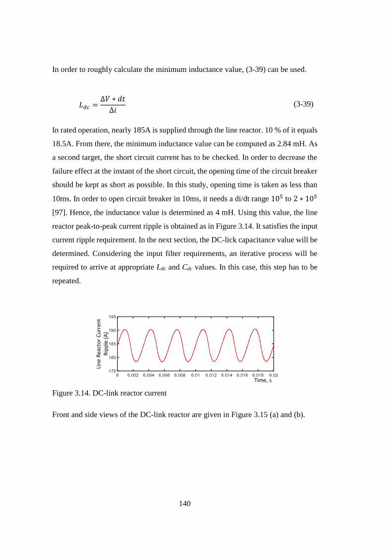
140

In order to roughly calculate the minimum inductance value, (3-39) can be used.

𝐿𝑑𝑐 =

∆𝑉 ∗ 𝑑𝑡

∆𝑖 (3-39)

In rated operation, nearly 185A is supplied through the line reactor. 10 % of it equals

18.5A. From there, the minimum inductance value can be computed as 2.84 mH. As

a second target, the short circuit current has to be checked. In order to decrease the

failure effect at the instant of the short circuit, the opening time of the circuit breaker

should be kept as short as possible. In this study, opening time is taken as less than

10ms. In order to open circuit breaker in 10ms, it needs a di/dt range 105 to 2 ∗ 105

[97]. Hence, the inductance value is determined as 4 mH. Using this value, the line

reactor peak-to-peak current ripple is obtained as in Figure 3.14. It satisfies the input

current ripple requirement. In the next section, the DC-lick capacitance value will be

determined. Considering the input filter requirements, an iterative process will be

required to arrive at appropriate Ldc and Cdc values. In this case, this step has to be

repeated.

Lin

e R

eact

or

Cu

rren

t R

ipp

le (

A)

Time, s

Figure 3.14. DC-link reactor current

Front and side views of the DC-link reactor are given in Figure 3.15 (a) and (b).

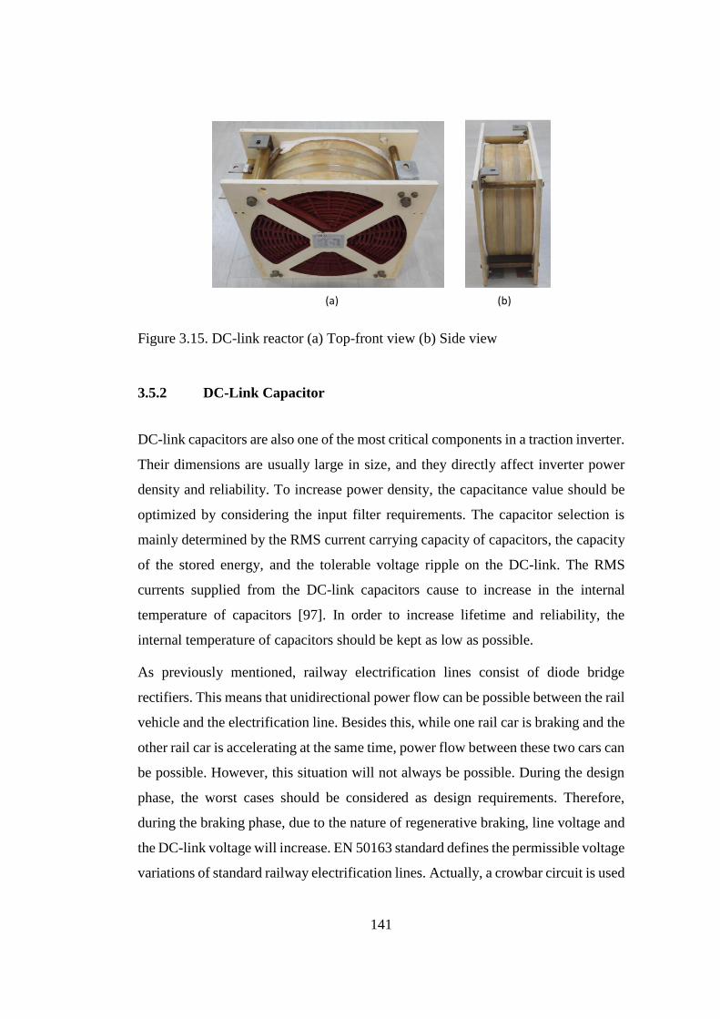
141

(a) (b)

Figure 3.15. DC-link reactor (a) Top-front view (b) Side view

3.5.2 DC-Link Capacitor

DC-link capacitors are also one of the most critical components in a traction inverter.

Their dimensions are usually large in size, and they directly affect inverter power

density and reliability. To increase power density, the capacitance value should be

optimized by considering the input filter requirements. The capacitor selection is

mainly determined by the RMS current carrying capacity of capacitors, the capacity

of the stored energy, and the tolerable voltage ripple on the DC-link. The RMS

currents supplied from the DC-link capacitors cause to increase in the internal

temperature of capacitors [97]. In order to increase lifetime and reliability, the

internal temperature of capacitors should be kept as low as possible.

As previously mentioned, railway electrification lines consist of diode bridge

rectifiers. This means that unidirectional power flow can be possible between the rail

vehicle and the electrification line. Besides this, while one rail car is braking and the

other rail car is accelerating at the same time, power flow between these two cars can

be possible. However, this situation will not always be possible. During the design

phase, the worst cases should be considered as design requirements. Therefore,

during the braking phase, due to the nature of regenerative braking, line voltage and

the DC-link voltage will increase. EN 50163 standard defines the permissible voltage

variations of standard railway electrification lines. Actually, a crowbar circuit is used

142

to limit the voltage increase. However, there should be a voltage margin to enable

this circuit. This voltage limit should be out of normal working voltage ranges. This

means the activation voltage of the crowbar circuit should be higher than the upper

level of nominal working voltage. In this study, 910 VDC was set for crowbar circuit

activation. This fact should also be considered during the design phase. This also has

to be taken into account for the selection of DC-link capacitors.

Following criteria should be considered for the selection of DC-link capacitors;

Nominal and peak voltages considering with the exposure times,

Harmonic current ratings in steady-state and transient operations,

Lifetime,

Thermal stresses,

DC-link voltage ripple due to railway electrification line voltage ripple and

high frequency ripple current caused from switching nature of the traction

inverter considering the reactive power need,

Capacitor energy has to sustain output power demand during short periods at

the instant of energy interruptions,

The capacitance value should be enough for expected dynamic load

variations (e.g., At the emergency stop condition, the torque is immediately

set to zero, and all power switches are made off within a very short time

period. The stored energy on the line reactor or at the braking instant the

stored energy on the stator windings flows through the DC-link capacitor).

In previous sections, 𝐿𝑑𝑐 and resonance frequency 𝑓0 were determined as 4 mH and

32.8 Hz, respectively. Using (3-40), Cdc is computed as 5.9 mF.

𝐶𝑑𝑐 = 1/[(2𝜋𝑓0)

2𝐿𝑑𝑐] (3-40)

By using these Ldc and Cdc values, simulations are performed again, and DC-link

voltage ripple and DC-link capacitor current ripple values are investigated.

Simulation results are plotted in Figure 3.16 and Figure 3.17. Because of the LC

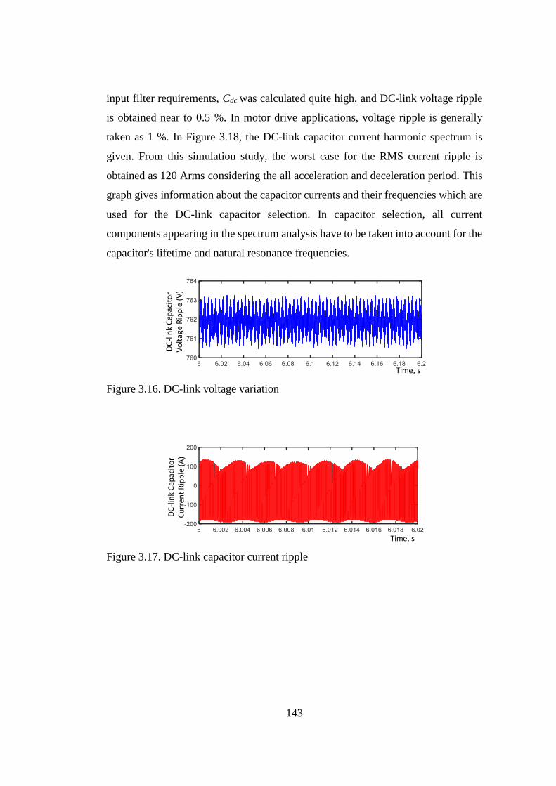
143

input filter requirements, Cdc was calculated quite high, and DC-link voltage ripple

is obtained near to 0.5 %. In motor drive applications, voltage ripple is generally

taken as 1 %. In Figure 3.18, the DC-link capacitor current harmonic spectrum is

given. From this simulation study, the worst case for the RMS current ripple is

obtained as 120 Arms considering the all acceleration and deceleration period. This

graph gives information about the capacitor currents and their frequencies which are

used for the DC-link capacitor selection. In capacitor selection, all current

components appearing in the spectrum analysis have to be taken into account for the

capacitor's lifetime and natural resonance frequencies.

DC

-lin

k C

apac

ito

r V

olt

age

Rip

ple

(V

)

Time, s

Figure 3.16. DC-link voltage variation

DC

-lin

k C

apac

ito

r C

urr

ent

Rip

ple

(A

)

Time, s

Figure 3.17. DC-link capacitor current ripple

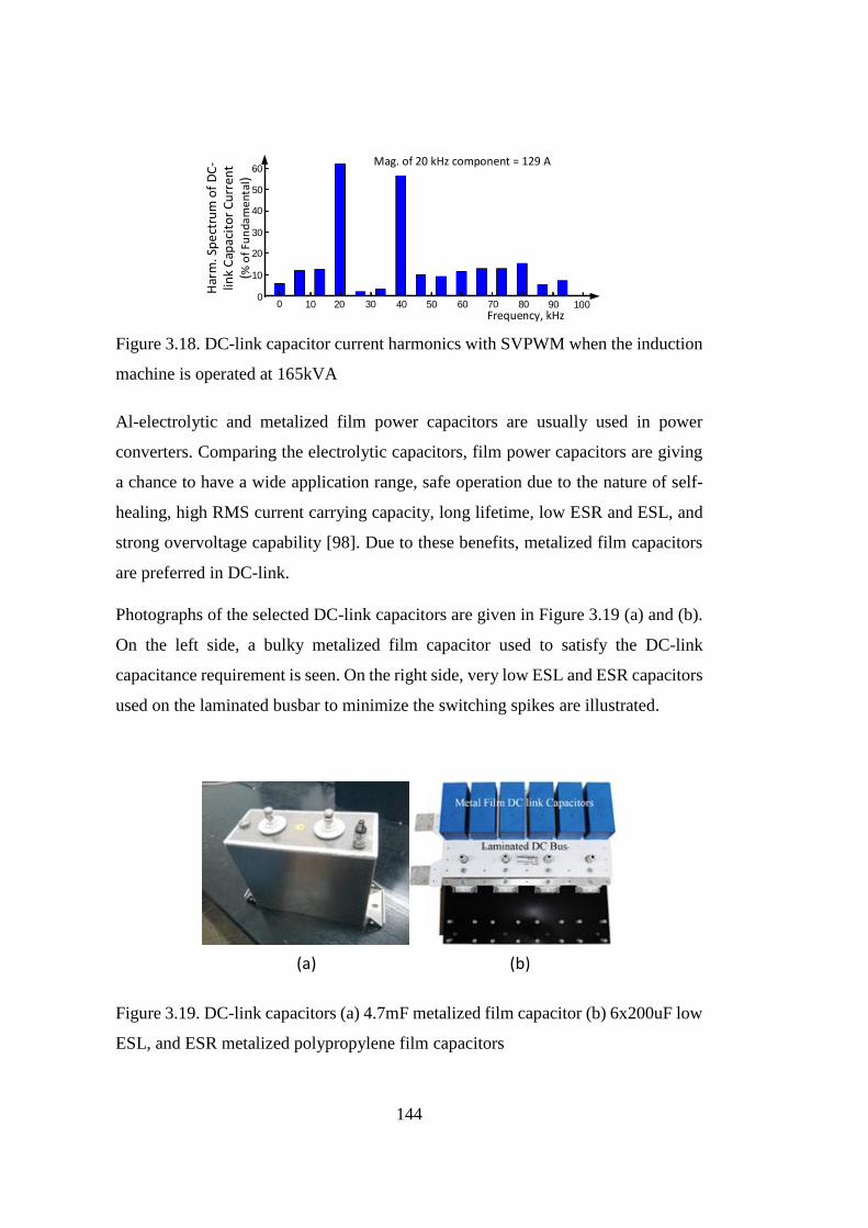
144

Har

m. S

pe

ctru

m o

f D

C-

link

Cap

acit

or

Cu

rren

t (%

of

Fun

da

me

nta

l)

Mag. of 20 kHz component = 129 A

Frequency, kHz0 10

0

60

40

20

10

20 30 40 50 60 70 80 90 100

30

50

Figure 3.18. DC-link capacitor current harmonics with SVPWM when the induction

machine is operated at 165kVA

Al-electrolytic and metalized film power capacitors are usually used in power

converters. Comparing the electrolytic capacitors, film power capacitors are giving

a chance to have a wide application range, safe operation due to the nature of self-

healing, high RMS current carrying capacity, long lifetime, low ESR and ESL, and

strong overvoltage capability [98]. Due to these benefits, metalized film capacitors

are preferred in DC-link.

Photographs of the selected DC-link capacitors are given in Figure 3.19 (a) and (b).

On the left side, a bulky metalized film capacitor used to satisfy the DC-link

capacitance requirement is seen. On the right side, very low ESL and ESR capacitors

used on the laminated busbar to minimize the switching spikes are illustrated.

(a) (b)

Figure 3.19. DC-link capacitors (a) 4.7mF metalized film capacitor (b) 6x200uF low

ESL, and ESR metalized polypropylene film capacitors

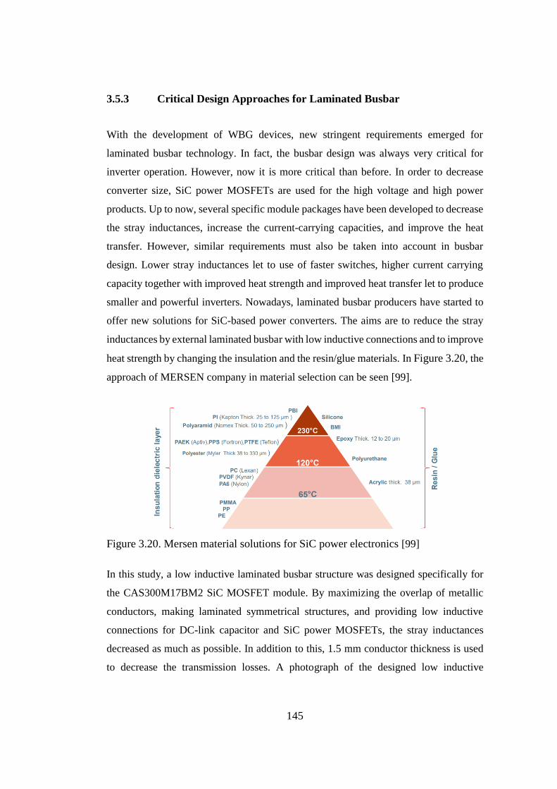
145

3.5.3 Critical Design Approaches for Laminated Busbar

With the development of WBG devices, new stringent requirements emerged for

laminated busbar technology. In fact, the busbar design was always very critical for

inverter operation. However, now it is more critical than before. In order to decrease

converter size, SiC power MOSFETs are used for the high voltage and high power

products. Up to now, several specific module packages have been developed to decrease

the stray inductances, increase the current-carrying capacities, and improve the heat

transfer. However, similar requirements must also be taken into account in busbar

design. Lower stray inductances let to use of faster switches, higher current carrying

capacity together with improved heat strength and improved heat transfer let to produce

smaller and powerful inverters. Nowadays, laminated busbar producers have started to

offer new solutions for SiC-based power converters. The aims are to reduce the stray

inductances by external laminated busbar with low inductive connections and to improve

heat strength by changing the insulation and the resin/glue materials. In Figure 3.20, the

approach of MERSEN company in material selection can be seen [99].

Figure 3.20. Mersen material solutions for SiC power electronics [99]

In this study, a low inductive laminated busbar structure was designed specifically for

the CAS300M17BM2 SiC MOSFET module. By maximizing the overlap of metallic

conductors, making laminated symmetrical structures, and providing low inductive

connections for DC-link capacitor and SiC power MOSFETs, the stray inductances

decreased as much as possible. In addition to this, 1.5 mm conductor thickness is used

to decrease the transmission losses. A photograph of the designed low inductive

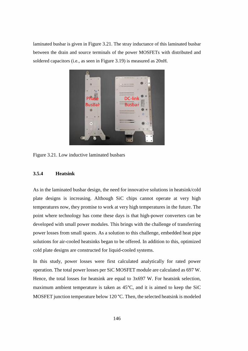
146

laminated busbar is given in Figure 3.21. The stray inductance of this laminated busbar

between the drain and source terminals of the power MOSFETs with distributed and

soldered capacitors (i.e., as seen in Figure 3.19) is measured as 20nH.

Phase Busbar

DC-link Busbar

Figure 3.21. Low inductive laminated busbars

3.5.4 Heatsink

As in the laminated busbar design, the need for innovative solutions in heatsink/cold

plate designs is increasing. Although SiC chips cannot operate at very high

temperatures now, they promise to work at very high temperatures in the future. The

point where technology has come these days is that high-power converters can be

developed with small power modules. This brings with the challenge of transferring

power losses from small spaces. As a solution to this challenge, embedded heat pipe

solutions for air-cooled heatsinks began to be offered. In addition to this, optimized

cold plate designs are constructed for liquid-cooled systems.

In this study, power losses were first calculated analytically for rated power

operation. The total power losses per SiC MOSFET module are calculated as 697 W.

Hence, the total losses for heatsink are equal to 3x697 W. For heatsink selection,

maximum ambient temperature is taken as 45°C, and it is aimed to keep the SiC

MOSFET junction temperature below 120 °C. Then, the selected heatsink is modeled

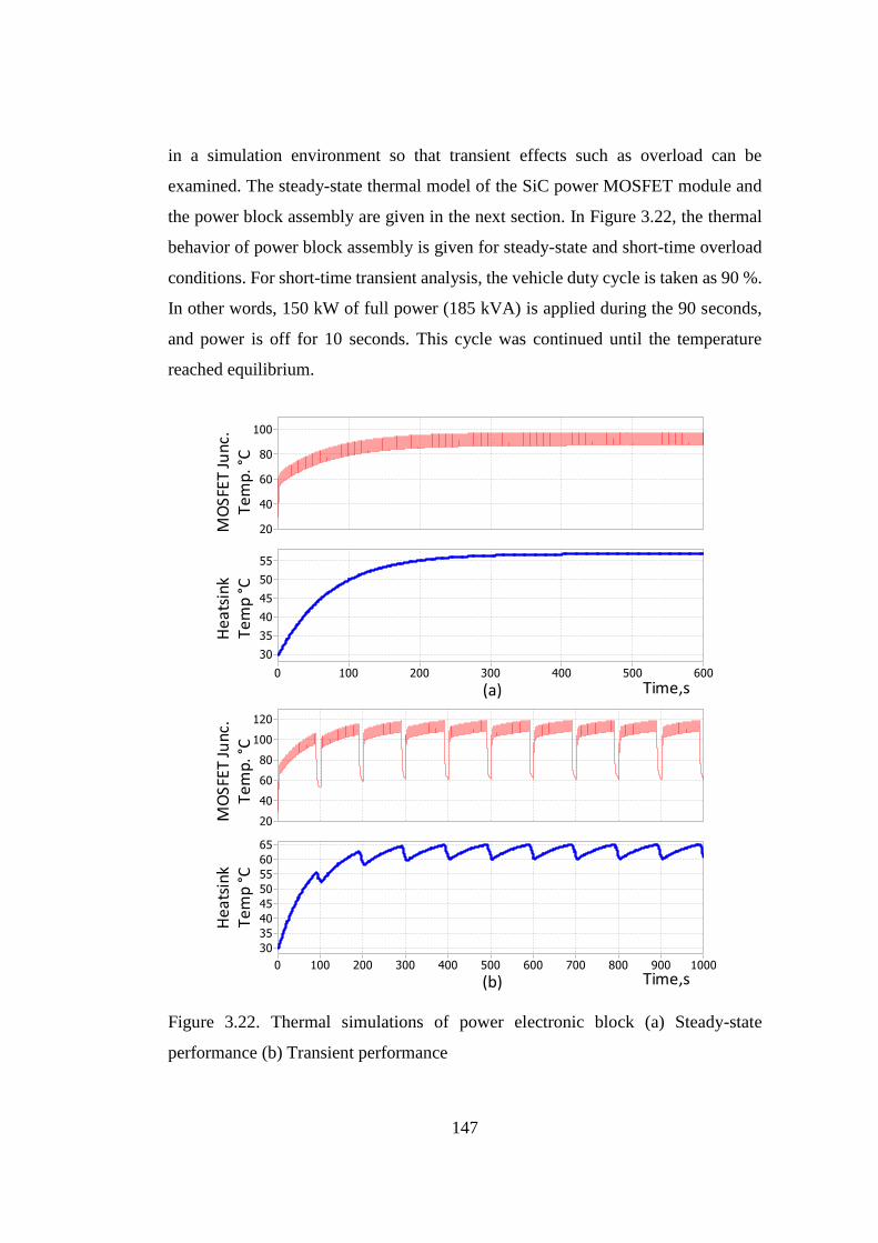
147

in a simulation environment so that transient effects such as overload can be

examined. The steady-state thermal model of the SiC power MOSFET module and

the power block assembly are given in the next section. In Figure 3.22, the thermal

behavior of power block assembly is given for steady-state and short-time overload

conditions. For short-time transient analysis, the vehicle duty cycle is taken as 90 %.

In other words, 150 kW of full power (185 kVA) is applied during the 90 seconds,

and power is off for 10 seconds. This cycle was continued until the temperature

reached equilibrium.

He

atsi

nk

Tem

p °

CM

OSF

ET Ju

nc.

Tem

p. °

C

Time,s(a)

Hea

tsin

k Te

mp

°CM

OSF

ET Ju

nc.

Tem

p. °

C

(b) Time,s

Figure 3.22. Thermal simulations of power electronic block (a) Steady-state

performance (b) Transient performance

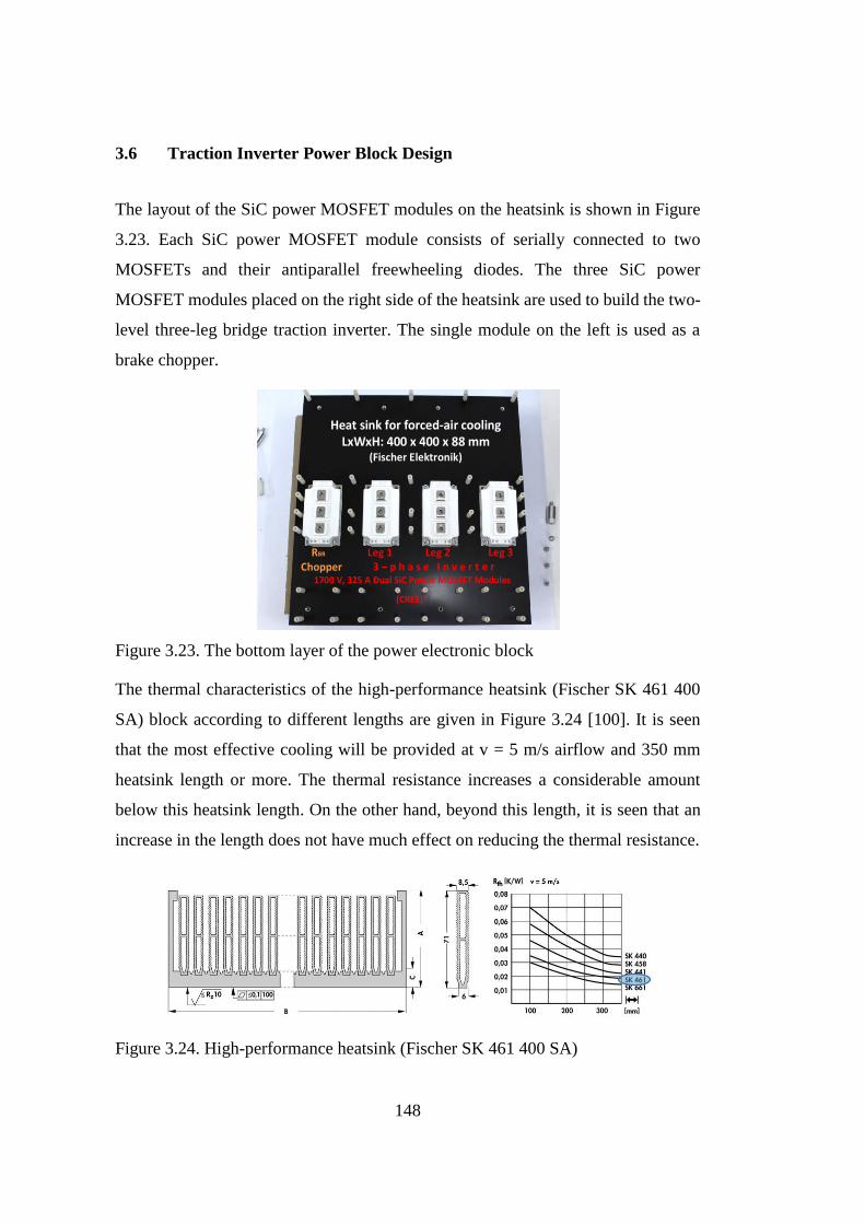
148

3.6 Traction Inverter Power Block Design

The layout of the SiC power MOSFET modules on the heatsink is shown in Figure

3.23. Each SiC power MOSFET module consists of serially connected to two

MOSFETs and their antiparallel freewheeling diodes. The three SiC power

MOSFET modules placed on the right side of the heatsink are used to build the two-

level three-leg bridge traction inverter. The single module on the left is used as a

brake chopper.

Heat sink for forced-air coolingLxWxH: 400 x 400 x 88 mm

(Fischer Elektronik)

RBR Leg 1 Chopper

Leg 2 Leg 3 3 – p h a s e I n v e r t e r

1700 V, 325 A Dual SiC Power MOSFET Modules

(CREE)

Figure 3.23. The bottom layer of the power electronic block

The thermal characteristics of the high-performance heatsink (Fischer SK 461 400

SA) block according to different lengths are given in Figure 3.24 [100]. It is seen

that the most effective cooling will be provided at v = 5 m/s airflow and 350 mm

heatsink length or more. The thermal resistance increases a considerable amount

below this heatsink length. On the other hand, beyond this length, it is seen that an

increase in the length does not have much effect on reducing the thermal resistance.

Figure 3.24. High-performance heatsink (Fischer SK 461 400 SA)

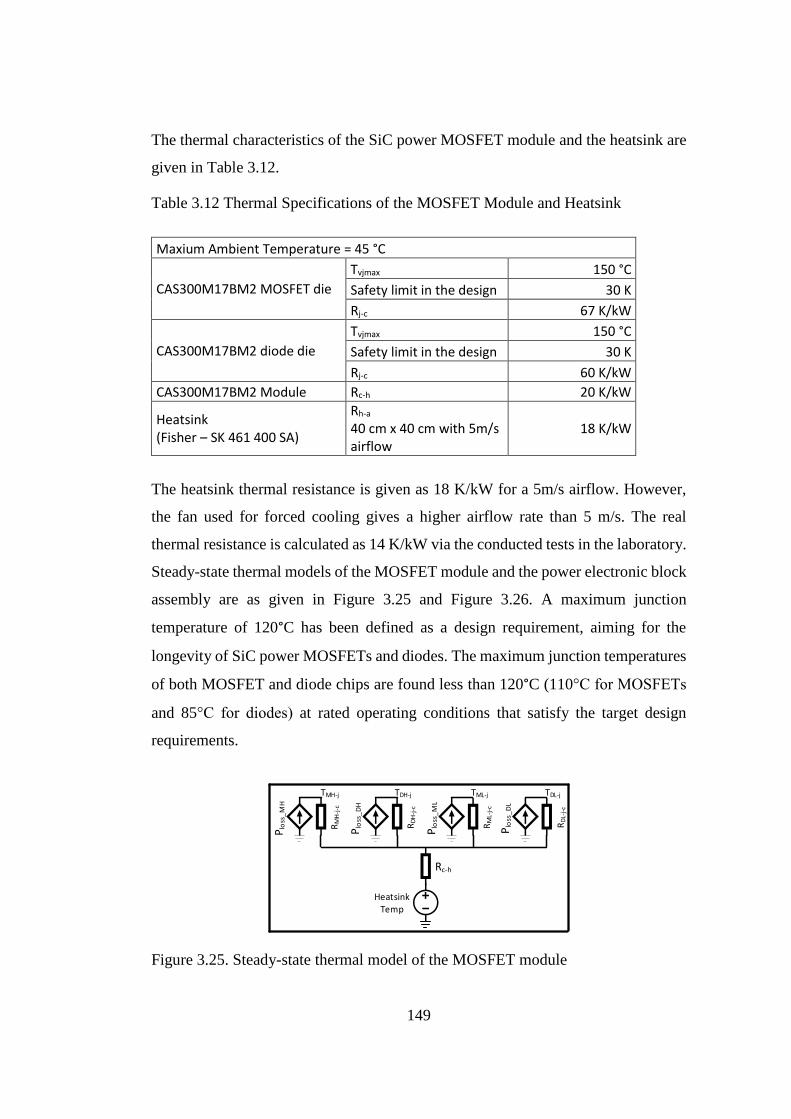
149

The thermal characteristics of the SiC power MOSFET module and the heatsink are

given in Table 3.12.

Table 3.12 Thermal Specifications of the MOSFET Module and Heatsink

Maxium Ambient Temperature = 45 °C

CAS300M17BM2 MOSFET die

Tvjmax 150 °C

Safety limit in the design 30 K

Rj-c 67 K/kW

CAS300M17BM2 diode die

Tvjmax 150 °C

Safety limit in the design 30 K

Rj-c 60 K/kW

CAS300M17BM2 Module Rc-h 20 K/kW

Heatsink (Fisher – SK 461 400 SA)

Rh-a

40 cm x 40 cm with 5m/s airflow

18 K/kW

The heatsink thermal resistance is given as 18 K/kW for a 5m/s airflow. However,

the fan used for forced cooling gives a higher airflow rate than 5 m/s. The real

thermal resistance is calculated as 14 K/kW via the conducted tests in the laboratory.

Steady-state thermal models of the MOSFET module and the power electronic block

assembly are as given in Figure 3.25 and Figure 3.26. A maximum junction

temperature of 120°C has been defined as a design requirement, aiming for the

longevity of SiC power MOSFETs and diodes. The maximum junction temperatures

of both MOSFET and diode chips are found less than 120°C (110°C for MOSFETs

and 85°C for diodes) at rated operating conditions that satisfy the target design

requirements.

Plo

ss_

MH

RM

H-j

-c

Plo

ss_

DH

RD

H-j

-c

Plo

ss_

ML

RM

L-j-

c

Plo

ss_

DL

RD

L-j-

c

Rc-h

Heatsink Temp

TMH-j TDH-j TML-j TDL-j

Figure 3.25. Steady-state thermal model of the MOSFET module

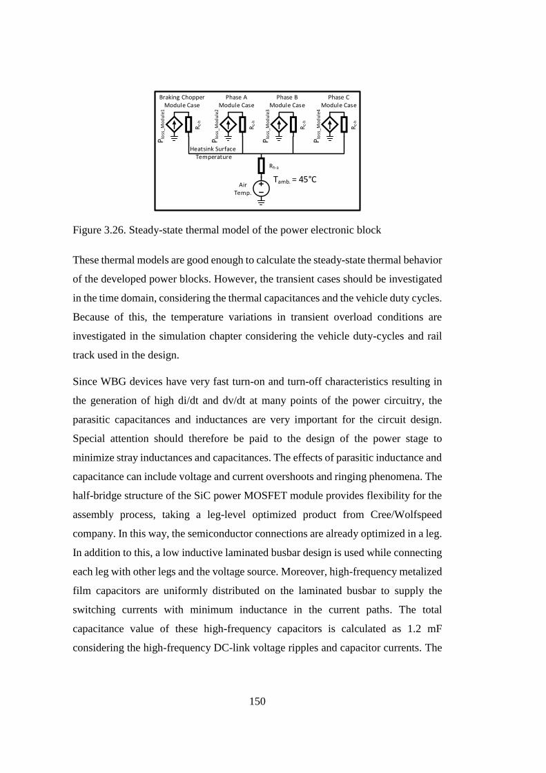
150

Tamb. = 45°C

Rh-a

Air Temp.

Plo

ss_

Mod

ule1

Rc-

h

Plo

ss_

Mod

ule3

Rc-

h

Plo

ss_

Mod

ule4

Rc-

h

Plo

ss_

Mod

ule2

Rc-

h

Heatsink Surface Temperature

Braking Chopper Module Case

Phase AModule Case

Phase BModule Case

Phase CModule Case

Figure 3.26. Steady-state thermal model of the power electronic block

These thermal models are good enough to calculate the steady-state thermal behavior

of the developed power blocks. However, the transient cases should be investigated

in the time domain, considering the thermal capacitances and the vehicle duty cycles.

Because of this, the temperature variations in transient overload conditions are

investigated in the simulation chapter considering the vehicle duty-cycles and rail

track used in the design.

Since WBG devices have very fast turn-on and turn-off characteristics resulting in

the generation of high di/dt and dv/dt at many points of the power circuitry, the

parasitic capacitances and inductances are very important for the circuit design.

Special attention should therefore be paid to the design of the power stage to

minimize stray inductances and capacitances. The effects of parasitic inductance and

capacitance can include voltage and current overshoots and ringing phenomena. The

half-bridge structure of the SiC power MOSFET module provides flexibility for the

assembly process, taking a leg-level optimized product from Cree/Wolfspeed

company. In this way, the semiconductor connections are already optimized in a leg.

In addition to this, a low inductive laminated busbar design is used while connecting

each leg with other legs and the voltage source. Moreover, high-frequency metalized

film capacitors are uniformly distributed on the laminated busbar to supply the

switching currents with minimum inductance in the current paths. The total

capacitance value of these high-frequency capacitors is calculated as 1.2 mF

considering the high-frequency DC-link voltage ripples and capacitor currents. The

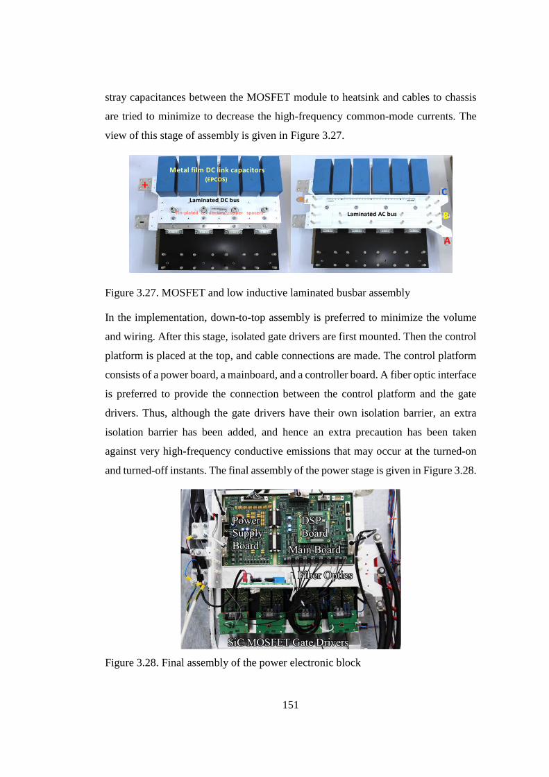
151

stray capacitances between the MOSFET module to heatsink and cables to chassis

are tried to minimize to decrease the high-frequency common-mode currents. The

view of this stage of assembly is given in Figure 3.27.

Laminated DC bus

-

Metal film DC link capacitors(EPCOS)

Tin-plated conductive copper spacers

+RBR

A

B

C

Laminated AC bus

Figure 3.27. MOSFET and low inductive laminated busbar assembly

In the implementation, down-to-top assembly is preferred to minimize the volume

and wiring. After this stage, isolated gate drivers are first mounted. Then the control

platform is placed at the top, and cable connections are made. The control platform

consists of a power board, a mainboard, and a controller board. A fiber optic interface

is preferred to provide the connection between the control platform and the gate

drivers. Thus, although the gate drivers have their own isolation barrier, an extra

isolation barrier has been added, and hence an extra precaution has been taken

against very high-frequency conductive emissions that may occur at the turned-on

and turned-off instants. The final assembly of the power stage is given in Figure 3.28.

Figure 3.28. Final assembly of the power electronic block

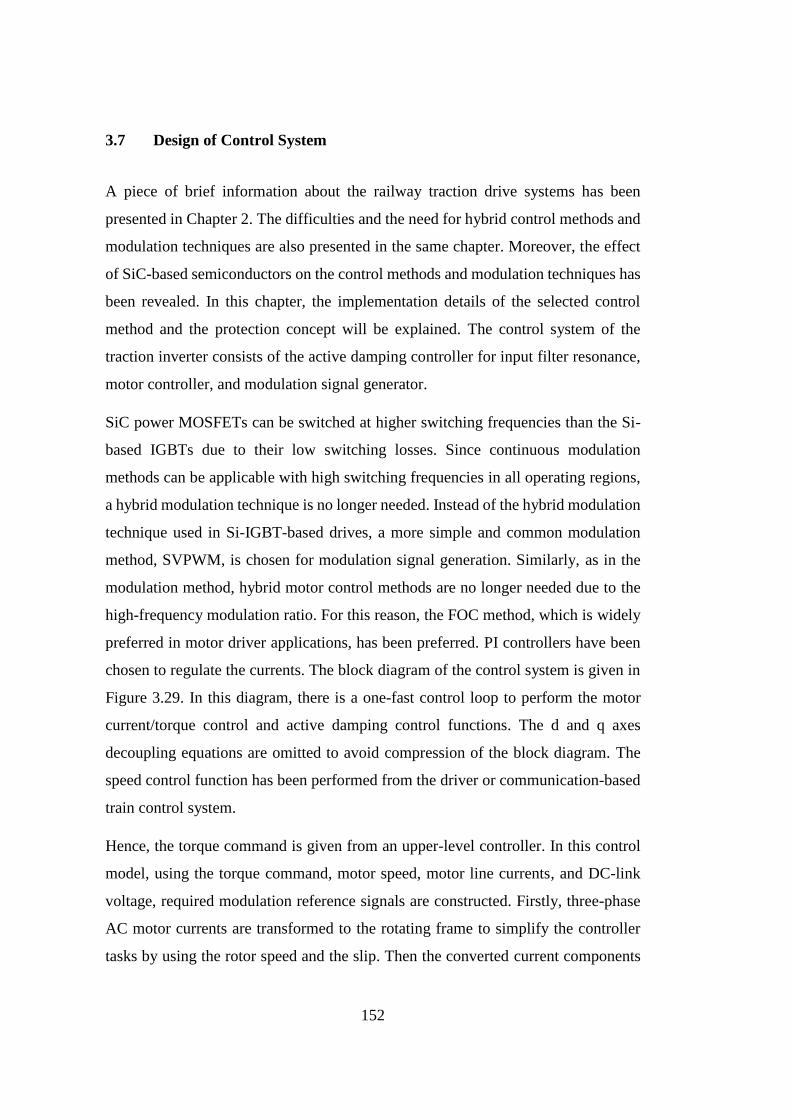
152

3.7 Design of Control System

A piece of brief information about the railway traction drive systems has been

presented in Chapter 2. The difficulties and the need for hybrid control methods and

modulation techniques are also presented in the same chapter. Moreover, the effect

of SiC-based semiconductors on the control methods and modulation techniques has

been revealed. In this chapter, the implementation details of the selected control

method and the protection concept will be explained. The control system of the

traction inverter consists of the active damping controller for input filter resonance,

motor controller, and modulation signal generator.

SiC power MOSFETs can be switched at higher switching frequencies than the Si-

based IGBTs due to their low switching losses. Since continuous modulation

methods can be applicable with high switching frequencies in all operating regions,

a hybrid modulation technique is no longer needed. Instead of the hybrid modulation

technique used in Si-IGBT-based drives, a more simple and common modulation

method, SVPWM, is chosen for modulation signal generation. Similarly, as in the

modulation method, hybrid motor control methods are no longer needed due to the

high-frequency modulation ratio. For this reason, the FOC method, which is widely

preferred in motor driver applications, has been preferred. PI controllers have been

chosen to regulate the currents. The block diagram of the control system is given in

Figure 3.29. In this diagram, there is a one-fast control loop to perform the motor

current/torque control and active damping control functions. The d and q axes

decoupling equations are omitted to avoid compression of the block diagram. The

speed control function has been performed from the driver or communication-based

train control system.

Hence, the torque command is given from an upper-level controller. In this control

model, using the torque command, motor speed, motor line currents, and DC-link

voltage, required modulation reference signals are constructed. Firstly, three-phase

AC motor currents are transformed to the rotating frame to simplify the controller

tasks by using the rotor speed and the slip. Then the converted current components

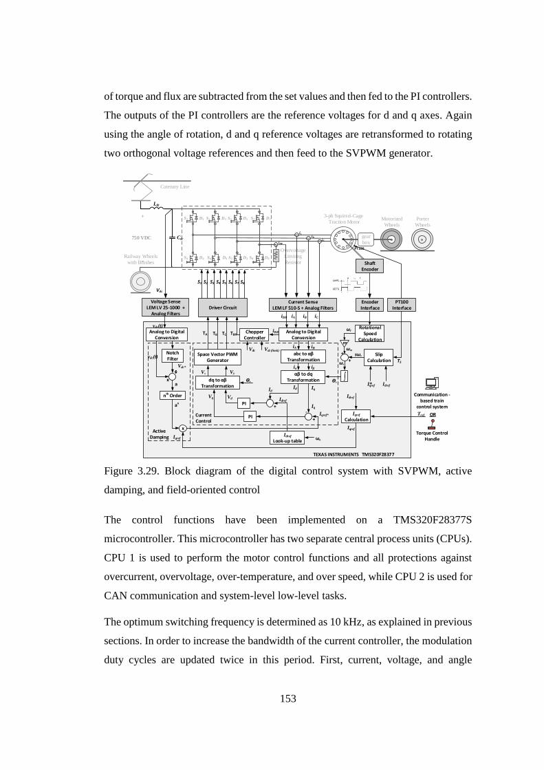
153

of torque and flux are subtracted from the set values and then fed to the PI controllers.

The outputs of the PI controllers are the reference voltages for d and q axes. Again

using the angle of rotation, d and q reference voltages are retransformed to rotating

two orthogonal voltage references and then feed to the SVPWM generator.

iA

Overvoltage

Limiting

Resistor

+

-

3-ph Squirrel-Cage

Traction MotorS1

Cdc

Ldc

D1

Catenary Line

Railway Wheels

with Brushes

Motorized

Wheels

gear

box750 VDC

Porter

Wheels

iB

iCiBR

S4 D4

S3 D3 S5 D5

S2 D2S6 D6

S7 D7

S8 D8

Space Vector PWMGenerator

Analog to Digital Conversion

abc to αβ Transformation

Id Iq

Idref

Iqref

+

+

-

-

dq to αβ Transformation

VdVq

Vα Vβ

Slip Calculation

ϴe

ωr

Tref

PI

PIIqref

Calculation

Idref

αβ to dq Transformation

iα iβ

iA

ϴe

ωe

Current Control

sωe

+

+ωre

S1 S2 S3 S4 S5 S6

TA TB TC

iB

Iq

iA iB iC

Analog to Digital Conversion

NotchFilter

x

nth Order

a

an

x

Iqref

Iqref*

vdc(t)

Vdc*

Idref

Look-up table

ActiveDamping

Id

S7 S8

Vdc

iBR

Chopper Controller

iBRTBR

Vdc(limit)

dd

Vdc

Voltage SenseLEM LV 25-1000 +

Analog FiltersDriver Circuit

Encoder Interface

TMS320F28377TEXAS INSTRUMENTS

Rotational Speed

Calculation

Shaft Encoder

Current Sense LEM LF 510-S + Analog Filters

IdrefI*qref

TS

PT100

PT100 Interface

ωe

OR

Torque Control Handle

Communication -based train

control system

vdc(t)

Figure 3.29. Block diagram of the digital control system with SVPWM, active

damping, and field-oriented control

The control functions have been implemented on a TMS320F28377S

microcontroller. This microcontroller has two separate central process units (CPUs).

CPU 1 is used to perform the motor control functions and all protections against

overcurrent, overvoltage, over-temperature, and over speed, while CPU 2 is used for

CAN communication and system-level low-level tasks.

The optimum switching frequency is determined as 10 kHz, as explained in previous

sections. In order to increase the bandwidth of the current controller, the modulation

duty cycles are updated twice in this period. First, current, voltage, and angle

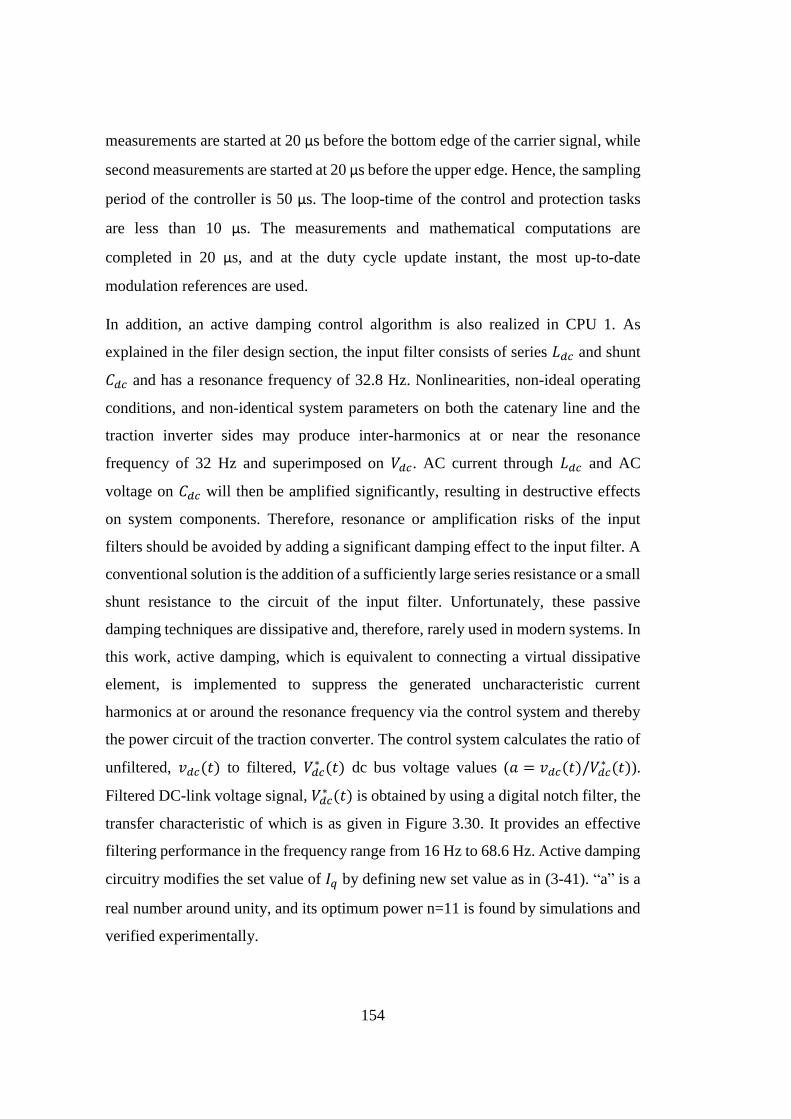
154

measurements are started at 20 µs before the bottom edge of the carrier signal, while

second measurements are started at 20 µs before the upper edge. Hence, the sampling

period of the controller is 50 µs. The loop-time of the control and protection tasks

are less than 10 µs. The measurements and mathematical computations are

completed in 20 µs, and at the duty cycle update instant, the most up-to-date

modulation references are used.

In addition, an active damping control algorithm is also realized in CPU 1. As

explained in the filer design section, the input filter consists of series 𝐿𝑑𝑐 and shunt

𝐶𝑑𝑐 and has a resonance frequency of 32.8 Hz. Nonlinearities, non-ideal operating

conditions, and non-identical system parameters on both the catenary line and the

traction inverter sides may produce inter-harmonics at or near the resonance

frequency of 32 Hz and superimposed on 𝑉𝑑𝑐. AC current through 𝐿𝑑𝑐 and AC

voltage on 𝐶𝑑𝑐 will then be amplified significantly, resulting in destructive effects

on system components. Therefore, resonance or amplification risks of the input

filters should be avoided by adding a significant damping effect to the input filter. A

conventional solution is the addition of a sufficiently large series resistance or a small

shunt resistance to the circuit of the input filter. Unfortunately, these passive

damping techniques are dissipative and, therefore, rarely used in modern systems. In

this work, active damping, which is equivalent to connecting a virtual dissipative

element, is implemented to suppress the generated uncharacteristic current

harmonics at or around the resonance frequency via the control system and thereby

the power circuit of the traction converter. The control system calculates the ratio of

unfiltered, 𝑣𝑑𝑐(𝑡) to filtered, 𝑉𝑑𝑐∗ (𝑡) dc bus voltage values (𝑎 = 𝑣𝑑𝑐(𝑡)/𝑉𝑑𝑐

∗ (𝑡)).

Filtered DC-link voltage signal, 𝑉𝑑𝑐∗ (𝑡) is obtained by using a digital notch filter, the

transfer characteristic of which is as given in Figure 3.30. It provides an effective

filtering performance in the frequency range from 16 Hz to 68.6 Hz. Active damping

circuitry modifies the set value of 𝐼𝑞 by defining new set value as in (3-41). “a” is a

real number around unity, and its optimum power n=11 is found by simulations and

verified experimentally.

155

𝐼𝑞𝑟𝑒𝑓∗ = 𝑎𝑛 𝐼𝑞𝑟𝑒𝑓 (3-41)

68.6

Hz

16

Hz

Input Filter

32.8

Hz

47.5

Hz

Digital Notch Filter

Frequency, Hz

Figure 3.30. Transfer characteristics of input power filter and digital notch filter

plotted against the same frequency range

Harmonic frequencies lower than 68.6 Hz are successfully suppressed by active

filtering action via digital notch filter. Low order and high-frequency harmonics

outside the frequency band defined above (e.g., 0 - 68.6 Hz), including switching

frequency, its sidebands, and multiples, appearing on both catenary and traction

sides, are successfully suppressed by the input filter.

157

CHAPTER 4

4 MODELING OF ELECTRIC TRACTION DRIVE SYSTEM

In this chapter, first, the LTspice model was created to investigate the switching

performance of the SiC MOSFET Module CAS300M17BM2. Then,

MATLAB/Simulink models for simulation of light rail transportation vehicle and its

traction drive system are developed, and simulation results are presented. These two

models are performed in separate simulation tasks because of the simulation sample

time and duration needs. In the vehicle simulation model, track data, vehicle weight,

wheel diameters, adhesion coefficient, train resistance, acceleration/deceleration

rates, operating duty cycles are taken into account, and traction system requirements

are analyzed. Besides this, in the traction drive system model, power electronic-

based simulations are performed to analyze the system response together with the

hardware and control system. The whole system model consists of a 6 and 12 pulse

diode rectifier electrification system, a three-phase two-level voltage source rectifier,

a three-phase two-level voltage source traction inverter, a three-phase asynchronous

traction motor, and a control system. The electrical power system model is

implemented by using Simulink/Simpower System Toolbox. Besides, the standard

block sets of Simulink are used to construct the control system. These two different

discipline can be easily incorporated. The separation between the control system and

the converter power stage allows the user to simulate and analyze the complex

systems easily. During the simulations, field-oriented control and V/Hz scalar

control methods are utilized. The SVPWM modulation technique is implemented.

The purpose of the simulations is to see the characteristics of the whole traction drive

system and optimize it before the hardware design stage is completed. In addition to

this, SHEM is also implemented to make an additional comparison. Finally, a

PLECS model is developed to investigate the thermal variations of semiconductors

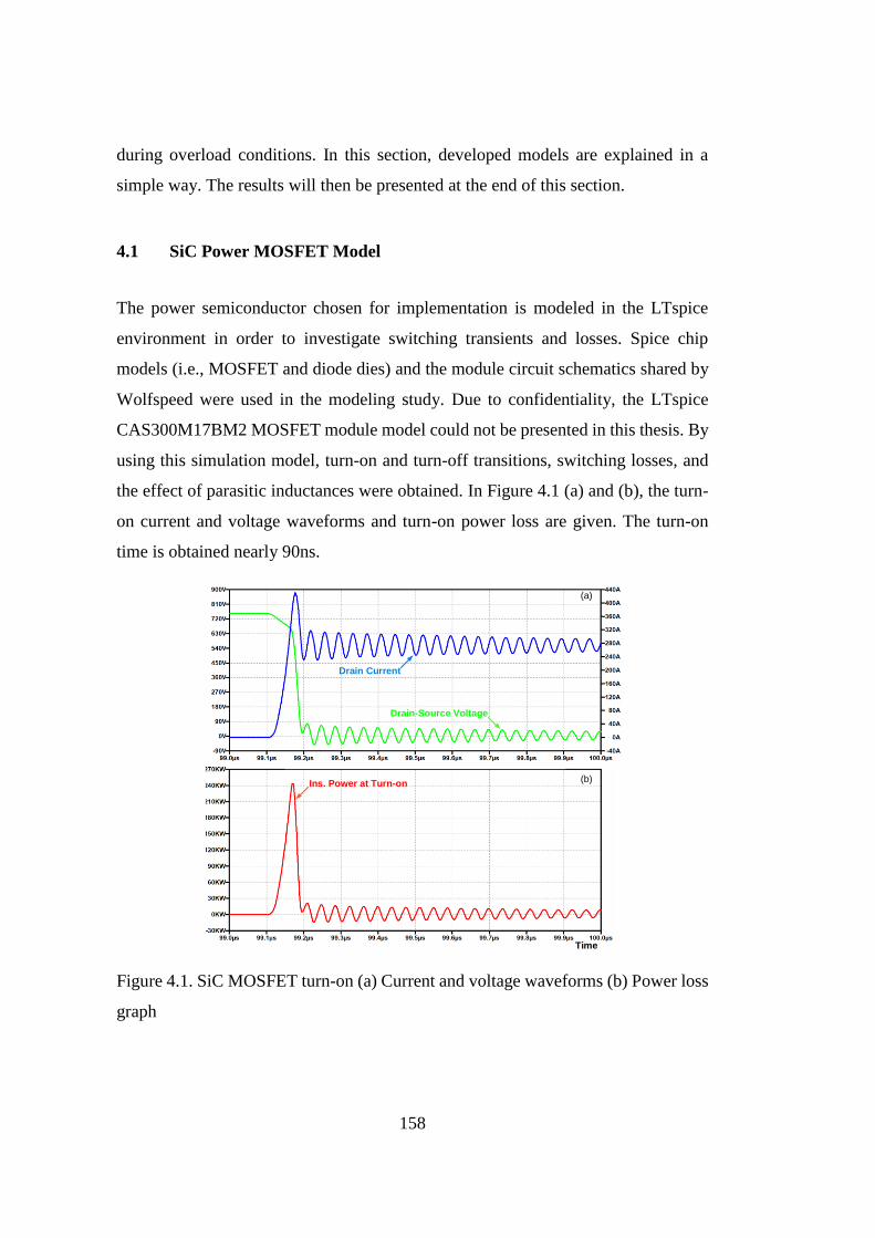
158

during overload conditions. In this section, developed models are explained in a

simple way. The results will then be presented at the end of this section.

4.1 SiC Power MOSFET Model

The power semiconductor chosen for implementation is modeled in the LTspice

environment in order to investigate switching transients and losses. Spice chip

models (i.e., MOSFET and diode dies) and the module circuit schematics shared by

Wolfspeed were used in the modeling study. Due to confidentiality, the LTspice

CAS300M17BM2 MOSFET module model could not be presented in this thesis. By

using this simulation model, turn-on and turn-off transitions, switching losses, and

the effect of parasitic inductances were obtained. In Figure 4.1 (a) and (b), the turn-

on current and voltage waveforms and turn-on power loss are given. The turn-on

time is obtained nearly 90ns.

Drain Current

Drain-Source Voltage

Ins. Power at Turn-on

Time

(a)

(b)

Figure 4.1. SiC MOSFET turn-on (a) Current and voltage waveforms (b) Power loss

graph

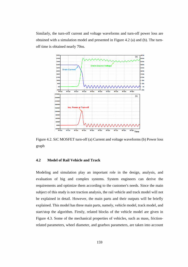
159

Similarly, the turn-off current and voltage waveforms and turn-off power loss are

obtained with a simulation model and presented in Figure 4.2 (a) and (b). The turn-

off time is obtained nearly 70ns.

Drain Current

Drain-Source Voltage

Ins. Power at Turn-off

Time

(a)

(b)

Figure 4.2. SiC MOSFET turn-off (a) Current and voltage waveforms (b) Power loss

graph

4.2 Model of Rail Vehicle and Track

Modeling and simulation play an important role in the design, analysis, and

evaluation of big and complex systems. System engineers can derive the

requirements and optimize them according to the customer's needs. Since the main

subject of this study is not traction analysis, the rail vehicle and track model will not

be explained in detail. However, the main parts and their outputs will be briefly

explained. This model has three main parts, namely, vehicle model, track model, and

start/stop the algorithm. Firstly, related blocks of the vehicle model are given in

Figure 4.3. Some of the mechanical properties of vehicles, such as mass, friction-

related parameters, wheel diameter, and gearbox parameters, are taken into account

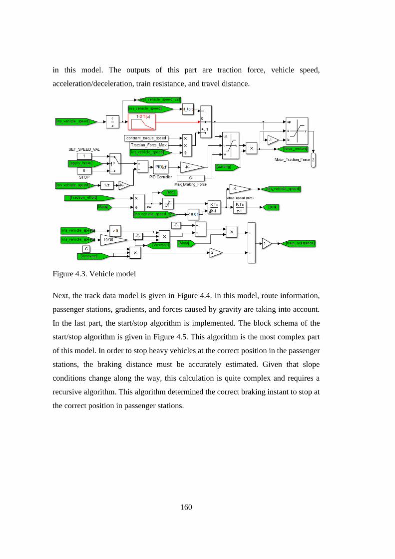
160

in this model. The outputs of this part are traction force, vehicle speed,

acceleration/deceleration, train resistance, and travel distance.

Figure 4.3. Vehicle model

Next, the track data model is given in Figure 4.4. In this model, route information,

passenger stations, gradients, and forces caused by gravity are taking into account.

In the last part, the start/stop algorithm is implemented. The block schema of the

start/stop algorithm is given in Figure 4.5. This algorithm is the most complex part

of this model. In order to stop heavy vehicles at the correct position in the passenger

stations, the braking distance must be accurately estimated. Given that slope

conditions change along the way, this calculation is quite complex and requires a

recursive algorithm. This algorithm determined the correct braking instant to stop at

the correct position in passenger stations.

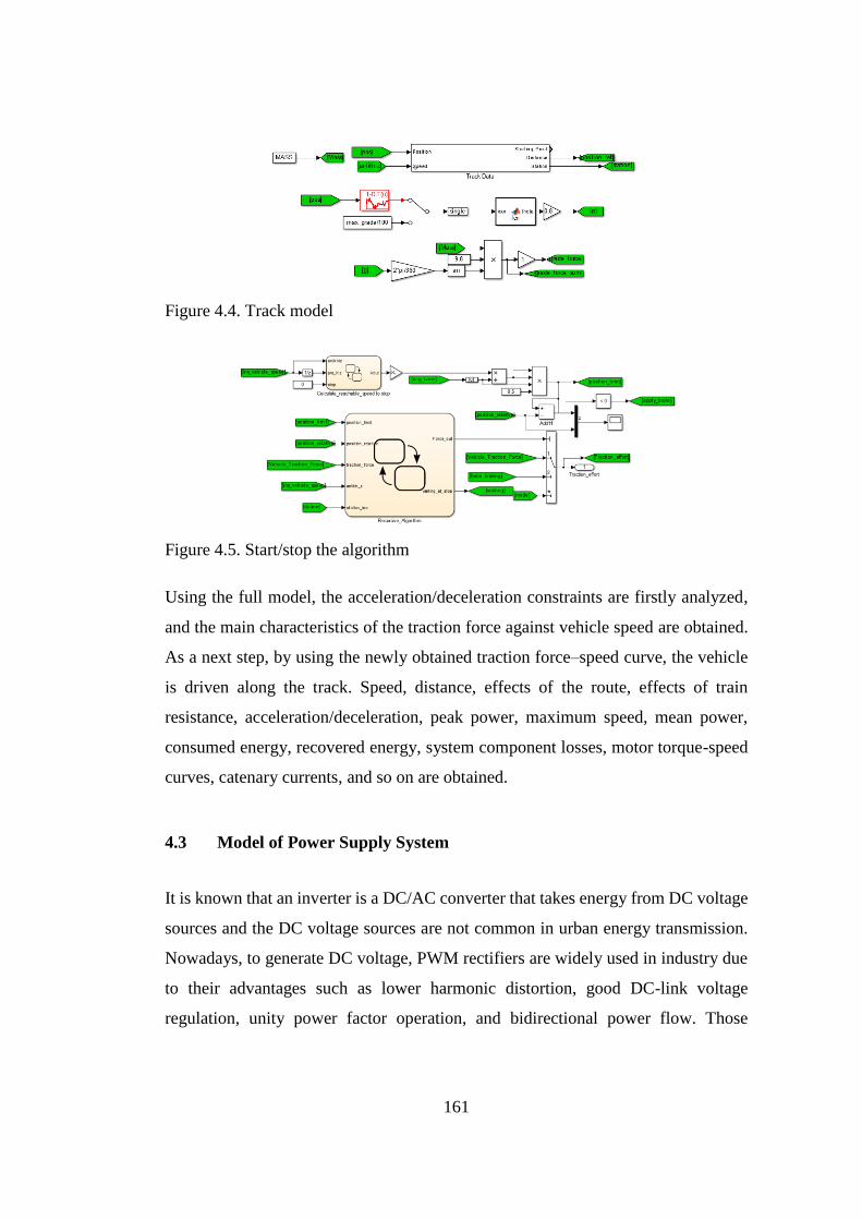
161

Figure 4.4. Track model

Figure 4.5. Start/stop the algorithm

Using the full model, the acceleration/deceleration constraints are firstly analyzed,

and the main characteristics of the traction force against vehicle speed are obtained.

As a next step, by using the newly obtained traction force–speed curve, the vehicle

is driven along the track. Speed, distance, effects of the route, effects of train

resistance, acceleration/deceleration, peak power, maximum speed, mean power,

consumed energy, recovered energy, system component losses, motor torque-speed

curves, catenary currents, and so on are obtained.

4.3 Model of Power Supply System

It is known that an inverter is a DC/AC converter that takes energy from DC voltage

sources and the DC voltage sources are not common in urban energy transmission.

Nowadays, to generate DC voltage, PWM rectifiers are widely used in industry due

to their advantages such as lower harmonic distortion, good DC-link voltage

regulation, unity power factor operation, and bidirectional power flow. Those

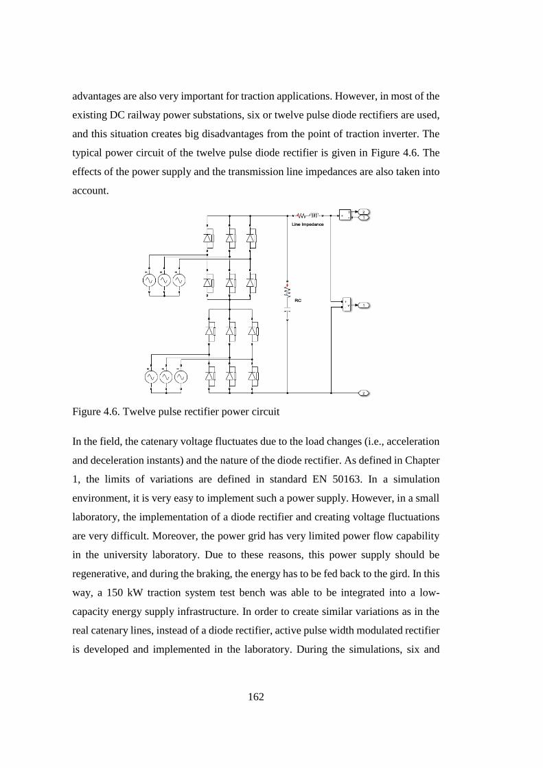
162

advantages are also very important for traction applications. However, in most of the

existing DC railway power substations, six or twelve pulse diode rectifiers are used,

and this situation creates big disadvantages from the point of traction inverter. The

typical power circuit of the twelve pulse diode rectifier is given in Figure 4.6. The

effects of the power supply and the transmission line impedances are also taken into

account.

Figure 4.6. Twelve pulse rectifier power circuit

In the field, the catenary voltage fluctuates due to the load changes (i.e., acceleration

and deceleration instants) and the nature of the diode rectifier. As defined in Chapter

1, the limits of variations are defined in standard EN 50163. In a simulation

environment, it is very easy to implement such a power supply. However, in a small

laboratory, the implementation of a diode rectifier and creating voltage fluctuations

are very difficult. Moreover, the power grid has very limited power flow capability

in the university laboratory. Due to these reasons, this power supply should be

regenerative, and during the braking, the energy has to be fed back to the gird. In this

way, a 150 kW traction system test bench was able to be integrated into a low-

capacity energy supply infrastructure. In order to create similar variations as in the

real catenary lines, instead of a diode rectifier, active pulse width modulated rectifier

is developed and implemented in the laboratory. During the simulations, six and

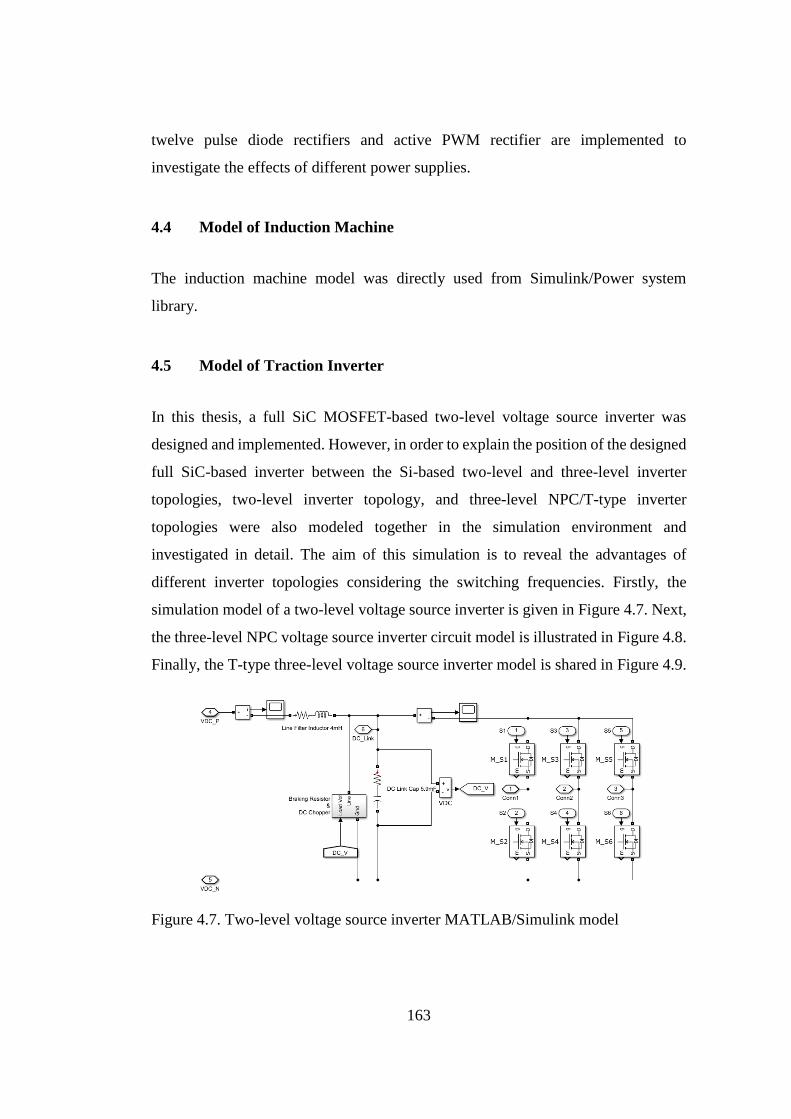
163

twelve pulse diode rectifiers and active PWM rectifier are implemented to

investigate the effects of different power supplies.

4.4 Model of Induction Machine

The induction machine model was directly used from Simulink/Power system

library.

4.5 Model of Traction Inverter

In this thesis, a full SiC MOSFET-based two-level voltage source inverter was

designed and implemented. However, in order to explain the position of the designed

full SiC-based inverter between the Si-based two-level and three-level inverter

topologies, two-level inverter topology, and three-level NPC/T-type inverter

topologies were also modeled together in the simulation environment and

investigated in detail. The aim of this simulation is to reveal the advantages of

different inverter topologies considering the switching frequencies. Firstly, the

simulation model of a two-level voltage source inverter is given in Figure 4.7. Next,

the three-level NPC voltage source inverter circuit model is illustrated in Figure 4.8.

Finally, the T-type three-level voltage source inverter model is shared in Figure 4.9.

Figure 4.7. Two-level voltage source inverter MATLAB/Simulink model

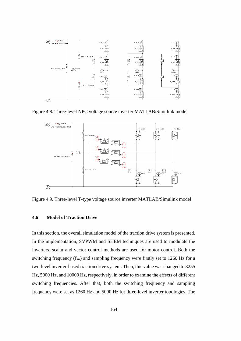
164

Figure 4.8. Three-level NPC voltage source inverter MATLAB/Simulink model

Figure 4.9. Three-level T-type voltage source inverter MATLAB/Simulink model

4.6 Model of Traction Drive

In this section, the overall simulation model of the traction drive system is presented.

In the implementation, SVPWM and SHEM techniques are used to modulate the

inverters, scalar and vector control methods are used for motor control. Both the

switching frequency (fsw) and sampling frequency were firstly set to 1260 Hz for a

two-level inverter-based traction drive system. Then, this value was changed to 3255

Hz, 5000 Hz, and 10000 Hz, respectively, in order to examine the effects of different

switching frequencies. After that, both the switching frequency and sampling

frequency were set as 1260 Hz and 5000 Hz for three-level inverter topologies. The

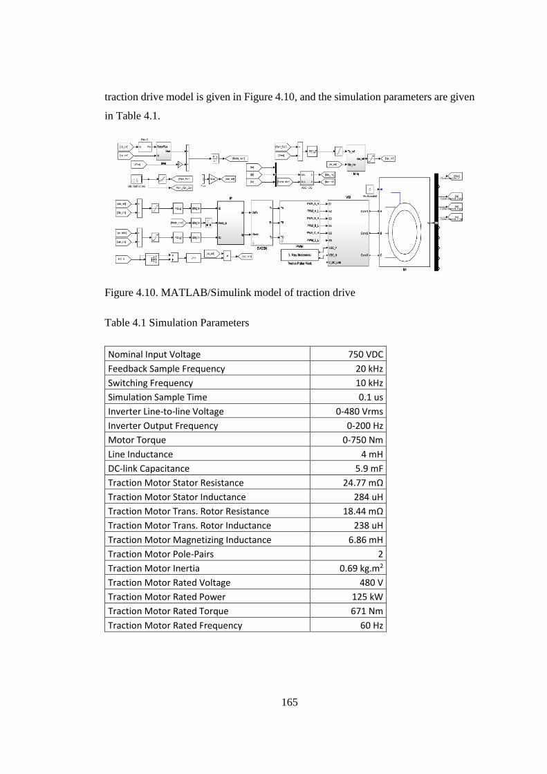
165

traction drive model is given in Figure 4.10, and the simulation parameters are given

in Table 4.1.

Figure 4.10. MATLAB/Simulink model of traction drive

Table 4.1 Simulation Parameters

Nominal Input Voltage 750 VDC

Feedback Sample Frequency 20 kHz

Switching Frequency 10 kHz

Simulation Sample Time 0.1 us

Inverter Line-to-line Voltage 0-480 Vrms

Inverter Output Frequency 0-200 Hz

Motor Torque 0-750 Nm

Line Inductance 4 mH

DC-link Capacitance 5.9 mF

Traction Motor Stator Resistance 24.77 mΩ

Traction Motor Stator Inductance 284 uH

Traction Motor Trans. Rotor Resistance 18.44 mΩ

Traction Motor Trans. Rotor Inductance 238 uH

Traction Motor Magnetizing Inductance 6.86 mH

Traction Motor Pole-Pairs 2

Traction Motor Inertia 0.69 kg.m2

Traction Motor Rated Voltage 480 V

Traction Motor Rated Power 125 kW

Traction Motor Rated Torque 671 Nm

Traction Motor Rated Frequency 60 Hz

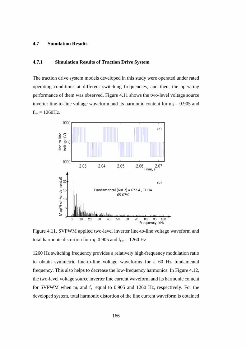
166

4.7 Simulation Results

4.7.1 Simulation Results of Traction Drive System

The traction drive system models developed in this study were operated under rated

operating conditions at different switching frequencies, and then, the operating

performance of them was observed. Figure 4.11 shows the two-level voltage source

inverter line-to-line voltage waveform and its harmonic content for mi = 0.905 and

fsw = 1260Hz.


Mag

(% o

f Fu

nda

men

tal)

Frequency, kHz0 10

0

20

15

10

5

20 30 40 50 60 70 80 90 100

Line

-to

-lin

e V

olta

ge (

V)

Time, s

(a)

(b)


total harmonic distortion for mi=0.905 and fsw = 1260 Hz

1260 Hz switching frequency provides a relatively high-frequency modulation ratio

to obtain symmetric line-to-line voltage waveforms for a 60 Hz fundamental

frequency. This also helps to decrease the low-frequency harmonics. In Figure 4.12,

the two-level voltage source inverter line current waveform and its harmonic content

for SVPWM when mi and fs equal to 0.905 and 1260 Hz, respectively. For the

developed system, total harmonic distortion of the line current waveform is obtained

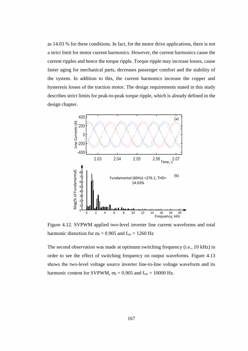
167

as 14.03 % for these conditions. In fact, for the motor drive applications, there is not

a strict limit for motor current harmonics. However, the current harmonics cause the

current ripples and hence the torque ripple. Torque ripple may increase losses, cause

faster aging for mechanical parts, decreases passenger comfort and the stability of

the system. In addition to this, the current harmonics increase the copper and

hysteresis losses of the traction motor. The design requirements stated in this study

describes strict limits for peak-to-peak torque ripple, which is already defined in the

design chapter.

Line

Cu

rren

ts (

A)

Time, s

(a)

(b)Fundamental (60Hz) =276.1, THD=

14.03%

Mag

(% o

f Fu

nda

men

tal)

Frequency, kHz0 2

0

7

1

4 6 8 10 12 14 16 18 20

2

3

4

5

6

8


harmonic distortion for mi = 0.905 and fsw = 1260 Hz

The second observation was made at optimum switching frequency (i.e., 10 kHz) in

order to see the effect of switching frequency on output waveforms. Figure 4.13

shows the two-level voltage source inverter line-to-line voltage waveform and its

harmonic content for SVPWM, mi = 0.905 and fsw = 10000 Hz.

168

Lin

e-t

o-l

ine

V

olt

age

(V

)

Time, s

(a)

(b)Fundamental (60Hz) = 675.47, THD=

64.06%

Mag

(% o

f Fu

nd

am

en

tal)

Frequency, kHz0 10

0

15

10

5

20 30 40 50 60 70 80 90 100


total harmonic distortion for SVPWM, mi = 0.905 and fsw = 10000 Hz

It is seen that the THD value of the line-to-line voltage is not affected by a significant

switching frequency increase. However, significant changes were obtained for the

frequency components of the line-to-line voltage harmonics. As can be followed

from Figure 4.11, all significant harmonics components were moved to higher

frequencies (i.e., components at switching frequency and integer multiples of it).

This will especially help to greatly reduce the motor current harmonics. In Figure

4.14, two-level voltage source inverter line current waveform and its harmonic

content for SVPWM at mi = 0.905 and fsw = 10000 Hz are given.

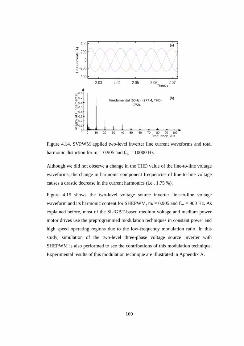
169

Line

Cu

rren

ts (

A)

Time, s

(a)


1.75%

Mag

(% o

f Fu

nda

men

tal)

Frequency, kHz0 10

0

0.7

0.1

20 30 40 50 60 70 80 90 100

0.2

0.3

0.4

0.5

0.6

0.8



Although we did not observe a change in the THD value of the line-to-line voltage

waveforms, the change in harmonic component frequencies of line-to-line voltage

causes a drastic decrease in the current harmonics (i.e., 1.75 %).

Figure 4.15 shows the two-level voltage source inverter line-to-line voltage

waveform and its harmonic content for SHEPWM, mi = 0.905 and fsw = 900 Hz. As

explained before, most of the Si-IGBT-based medium voltage and medium power

motor drives use the preprogrammed modulation techniques in constant power and

high speed operating regions due to the low-frequency modulation ratio. In this

study, simulation of the two-level three-phase voltage source inverter with

SHEPWM is also performed to see the contributions of this modulation technique.

Experimental results of this modulation technique are illustrated in Appendix A.

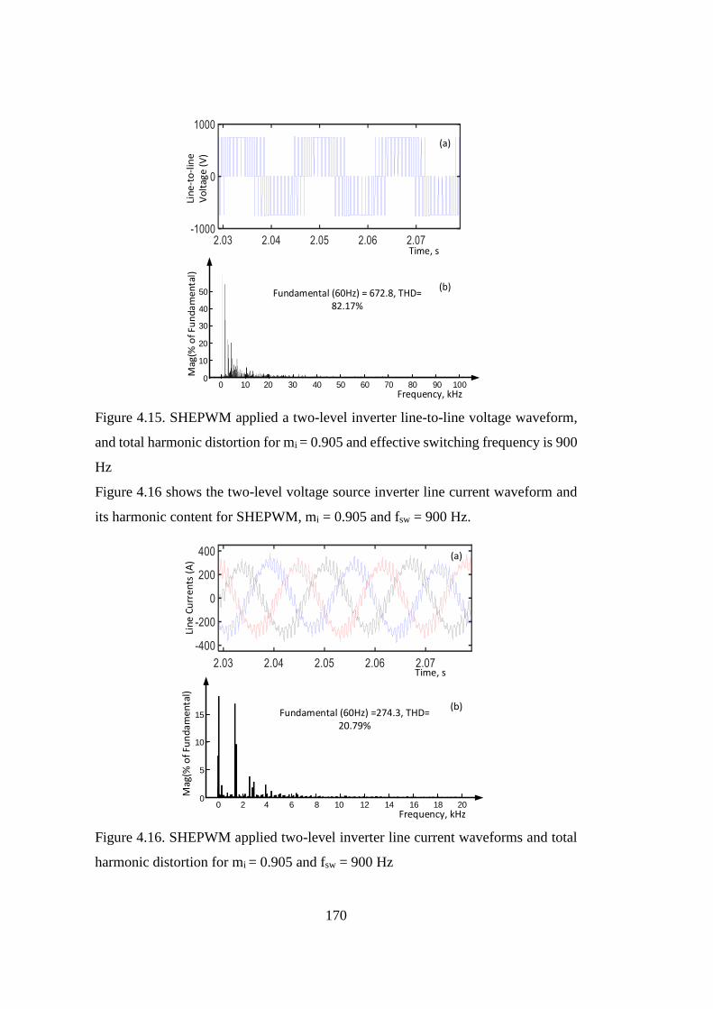
170

Lin

e-t

o-l

ine

V

olt

age

(V

)

Time, s

(a)

(b)Fundamental (60Hz) = 672.8, THD=

82.17%

Mag

(% o

f Fu

nd

am

en

tal)

Frequency, kHz0 10

0

20

10

20 30 40 50 60 70 80 90 100

30

40

50

Figure 4.15. SHEPWM applied a two-level inverter line-to-line voltage waveform,

and total harmonic distortion for mi = 0.905 and effective switching frequency is 900

Hz

Figure 4.16 shows the two-level voltage source inverter line current waveform and

its harmonic content for SHEPWM, mi = 0.905 and fsw = 900 Hz.

Line

Cu

rren

ts (

A)

Time, s

(a)


20.79%

Mag

(% o

f Fu

nd

am

enta

l)

Frequency, kHz0 2

04 6 8 10 12 14 16 18 20

5

10

15

Figure 4.16. SHEPWM applied two-level inverter line current waveforms and total


171

In addition to this, as explained in previous chapters, the medium voltage and

medium power two-level voltage source traction inverters suffer high losses that

increase with power and voltage levels. Because of this, the topology change is

needed between two-level and three-level inverter topologies. Three-level topologies

are superior to two-level topologies if the switching frequencies are relatively low.

This issue was already examined in the design chapter. However, this situation can

be changed if the switching frequencies can be increased. In this study, simulation

of the three-level three-phase voltage source inverter with SVPWM is also

performed in order to make a comparison between two-level and three-level three-

phase voltage source inverter topologies. In Figure 4.17, the three-level inverter line-

to-line voltage waveform and its THD are given at mi = 0.905 and fsw = 1260 Hz.

Lin

e-t

o-l

ine

V

olt

age

(V

)

Time, s

(a)

(b)

Fundamental (60Hz) = 671.6, THD= 34.34%

Mag

(% o

f Fu

nd

am

en

tal)

Frequency, kHz0 10

0

4

2

20 30 40 50 60 70 80 90 100

6

8

10

12

14


total harmonic distortion for mi = 0.905 and fsw = 1260 Hz

A significant improvement in the line-to-line voltage waveform has been achieved

compared to the result obtained with the two-level inverter. Here, the THD of the

line-to-line voltage is decreased a considerable amount, and the frequency content is

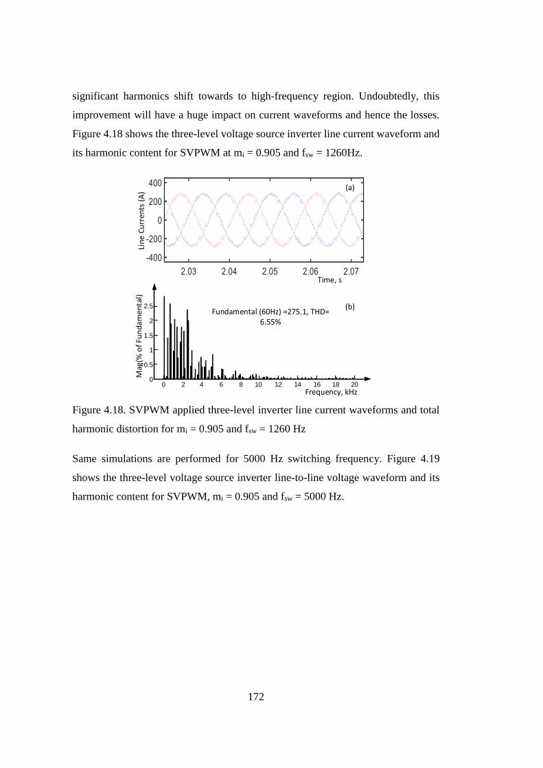
172

significant harmonics shift towards to high-frequency region. Undoubtedly, this

improvement will have a huge impact on current waveforms and hence the losses.

Figure 4.18 shows the three-level voltage source inverter line current waveform and

its harmonic content for SVPWM at mi = 0.905 and fsw = 1260Hz.

Lin

e C

urr

en

ts (

A)

Time, s

(a)


6.55%

Mag

(% o

f Fu

nd

am

en

tal)

Frequency, kHz0 2

0

0.5

4 6 8 10 12 14 16 18 20

1

1.5

2

2.5

Figure 4.18. SVPWM applied three-level inverter line current waveforms and total


Same simulations are performed for 5000 Hz switching frequency. Figure 4.19

shows the three-level voltage source inverter line-to-line voltage waveform and its

harmonic content for SVPWM, mi = 0.905 and fsw = 5000 Hz.

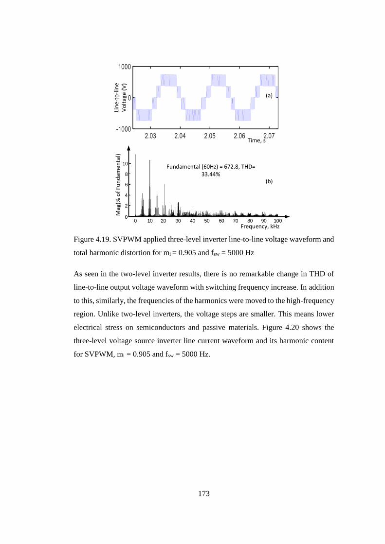
173

Lin

e-t

o-l

ine

V

olt

age

(V

)

Time, s

(a)

(b)

Fundamental (60Hz) = 672.8, THD= 33.44%

Mag

(% o

f Fu

nd

am

en

tal)

Frequency, kHz0 10

0

4

2

20 30 40 50 60 70 80 90 100

6

8

10


total harmonic distortion for mi = 0.905 and fsw = 5000 Hz

As seen in the two-level inverter results, there is no remarkable change in THD of

line-to-line output voltage waveform with switching frequency increase. In addition

to this, similarly, the frequencies of the harmonics were moved to the high-frequency

region. Unlike two-level inverters, the voltage steps are smaller. This means lower

electrical stress on semiconductors and passive materials. Figure 4.20 shows the

three-level voltage source inverter line current waveform and its harmonic content

for SVPWM, mi = 0.905 and fsw = 5000 Hz.

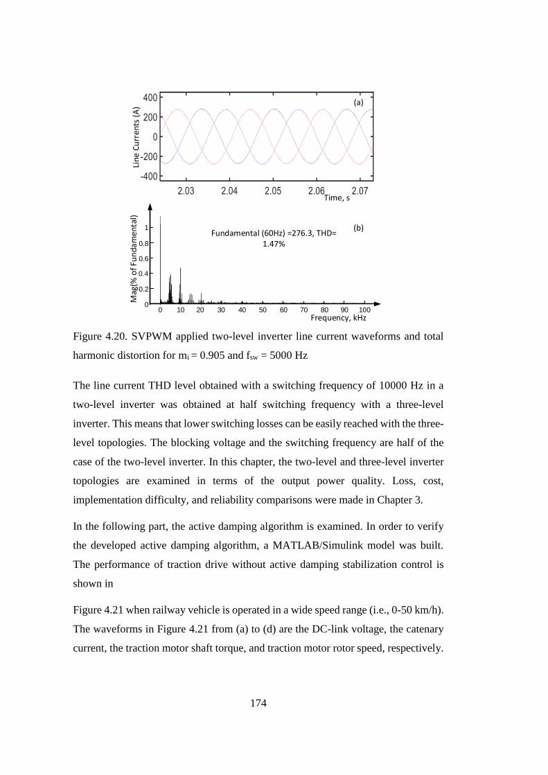
174

Lin

e C

urr

ents

(A

)

Time, s

(a)


1.47%

Mag

(% o

f Fu

nd

am

enta

l)

Frequency, kHz0 10

0

1

20 30 40 50 60 70 80 90 100

0.2

0.6

0.8

0.4



The line current THD level obtained with a switching frequency of 10000 Hz in a

two-level inverter was obtained at half switching frequency with a three-level

inverter. This means that lower switching losses can be easily reached with the three-

level topologies. The blocking voltage and the switching frequency are half of the

case of the two-level inverter. In this chapter, the two-level and three-level inverter

topologies are examined in terms of the output power quality. Loss, cost,

implementation difficulty, and reliability comparisons were made in Chapter 3.

In the following part, the active damping algorithm is examined. In order to verify

the developed active damping algorithm, a MATLAB/Simulink model was built.

The performance of traction drive without active damping stabilization control is

shown in

Figure 4.21 when railway vehicle is operated in a wide speed range (i.e., 0-50 km/h).

The waveforms in Figure 4.21 from (a) to (d) are the DC-link voltage, the catenary

current, the traction motor shaft torque, and traction motor rotor speed, respectively.

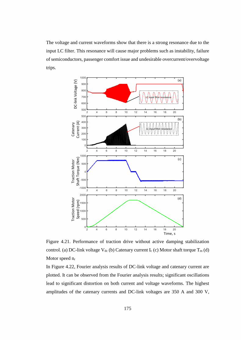
175

The voltage and current waveforms show that there is a strong resonance due to the

input LC filter. This resonance will cause major problems such as instability, failure

of semiconductors, passenger comfort issue and undesirable overcurrent/overvoltage

trips.

DC

-lin

k V

olt

age

(V)

Cat

enar

y C

urre

nt

(A)

Trac

tion

Mo

tor

Shaf

t To

rque

(N

m)

Trac

tion

Mo

tor

Spee

d (r

pm

)

Time, s

LC input filter resonance

LC input filter resonance

(a)

(b)

(c)

(d)


control. (a) DC-link voltage Vdc (b) Catenary current Ic (c) Motor shaft torque Tm (d)

Motor speed nr

In Figure 4.22, Fourier analysis results of DC-link voltage and catenary current are

plotted. It can be observed from the Fourier analysis results; significant oscillations

lead to significant distortion on both current and voltage waveforms. The highest

amplitudes of the catenary currents and DC-link voltages are 350 A and 300 V,

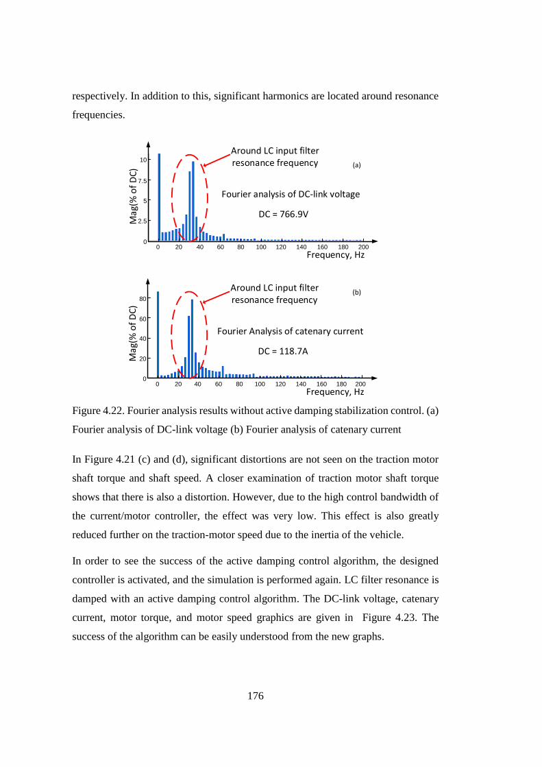
176

respectively. In addition to this, significant harmonics are located around resonance

frequencies.

DC = 766.9V

Mag

(% o

f D

C)

Frequency, Hz0 20

0

10

7.5

5

2.5

40 60 80 100 120 140 160 180 200

Fourier analysis of DC-link voltage

Around LC input filter resonance frequency

DC = 118.7A

Mag

(% o

f D

C)

Frequency, Hz0 20

0

80

60

40

20

40 60 80 100 120 140 160 180 200

Fourier Analysis of catenary current

Around LC input filter resonance frequency

(a)

(b)

Figure 4.22. Fourier analysis results without active damping stabilization control. (a)

Fourier analysis of DC-link voltage (b) Fourier analysis of catenary current

In Figure 4.21 (c) and (d), significant distortions are not seen on the traction motor

shaft torque and shaft speed. A closer examination of traction motor shaft torque

shows that there is also a distortion. However, due to the high control bandwidth of

the current/motor controller, the effect was very low. This effect is also greatly

reduced further on the traction-motor speed due to the inertia of the vehicle.

In order to see the success of the active damping control algorithm, the designed

controller is activated, and the simulation is performed again. LC filter resonance is

damped with an active damping control algorithm. The DC-link voltage, catenary

current, motor torque, and motor speed graphics are given in Figure 4.23. The

success of the algorithm can be easily understood from the new graphs.

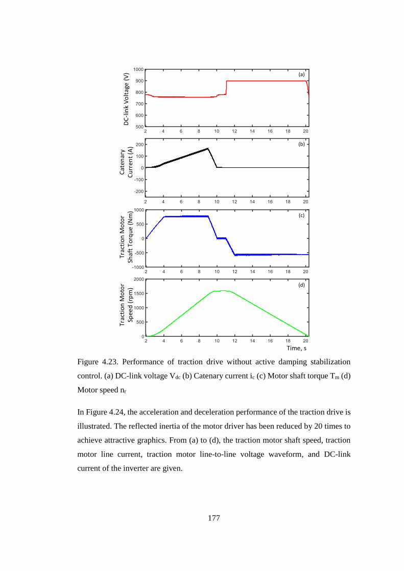
177

Time, s

DC

-lin

k V

olt

age

(V

)C

aten

ary

Cu

rren

t (A

)Tr

acti

on

Mo

tor

Shaf

t T

orq

ue

(N

m)

Trac

tio

n M

oto

r Sp

eed

(rp

m)

(a)

(b)

(c)

(d)


control. (a) DC-link voltage Vdc (b) Catenary current ic (c) Motor shaft torque Tm (d)

Motor speed nr

In Figure 4.24, the acceleration and deceleration performance of the traction drive is

illustrated. The reflected inertia of the motor driver has been reduced by 20 times to

achieve attractive graphics. From (a) to (d), the traction motor shaft speed, traction

motor line current, traction motor line-to-line voltage waveform, and DC-link

current of the inverter are given.

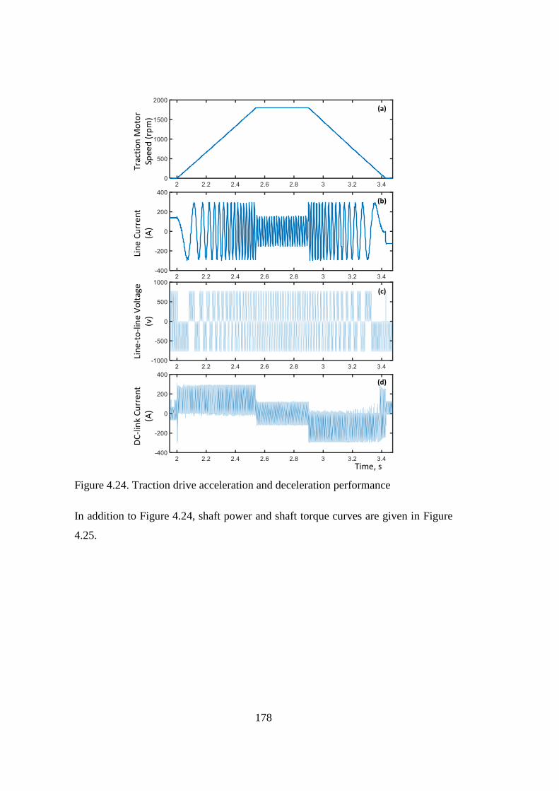
178

Trac

tio

n M

oto

r Sp

eed

(rp

m)

Lin

e C

urr

en

t (A

)Li

ne

-to

-lin

e V

olt

age

(v)

DC

-lin

k C

urr

en

t(A

)

Time, s

(a)

(b)

(c)

(d)

Figure 4.24. Traction drive acceleration and deceleration performance

In addition to Figure 4.24, shaft power and shaft torque curves are given in Figure

4.25.

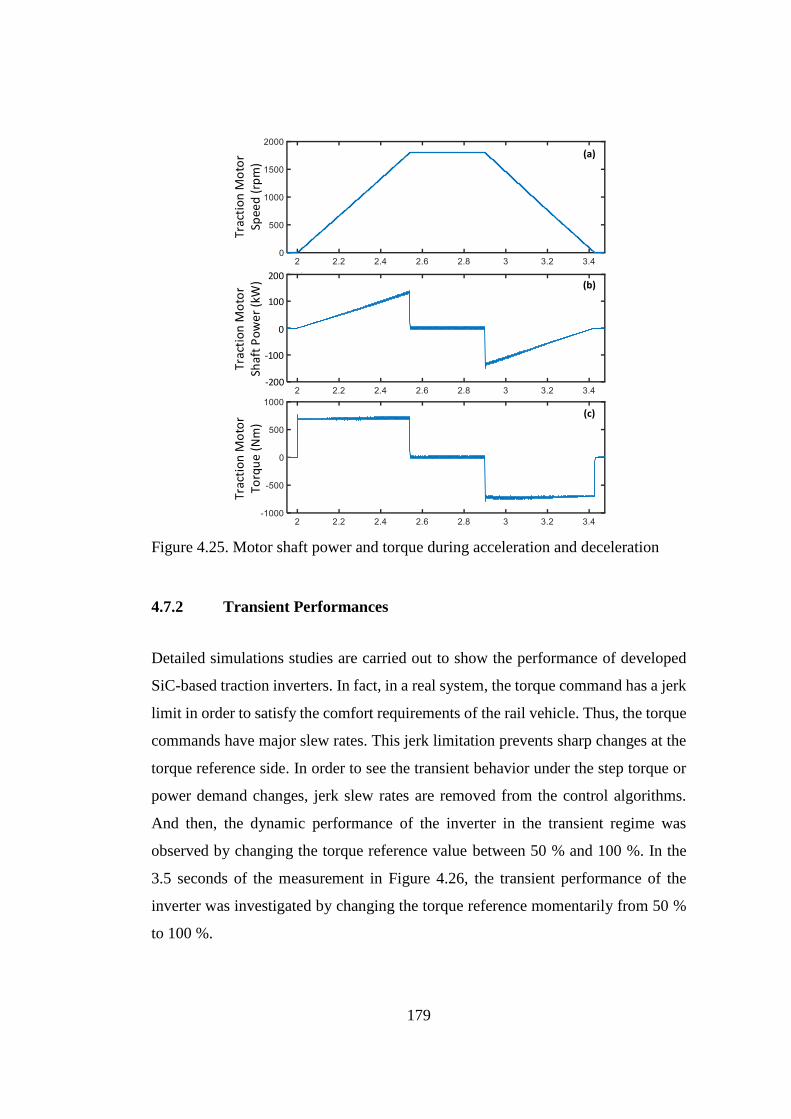
179

Trac

tio

n M

oto

r Sp

eed

(rp

m)

Trac

tio

n M

oto

r Sh

aft

Po

we

r (k

W)

0

100

200

-100

-200

Trac

tio

n M

oto

r To

rqu

e (N

m)

(a)

(b)

(c)

Figure 4.25. Motor shaft power and torque during acceleration and deceleration

4.7.2 Transient Performances

Detailed simulations studies are carried out to show the performance of developed

SiC-based traction inverters. In fact, in a real system, the torque command has a jerk

limit in order to satisfy the comfort requirements of the rail vehicle. Thus, the torque

commands have major slew rates. This jerk limitation prevents sharp changes at the

torque reference side. In order to see the transient behavior under the step torque or

power demand changes, jerk slew rates are removed from the control algorithms.

And then, the dynamic performance of the inverter in the transient regime was

observed by changing the torque reference value between 50 % and 100 %. In the

3.5 seconds of the measurement in Figure 4.26, the transient performance of the

inverter was investigated by changing the torque reference momentarily from 50 %

to 100 %.

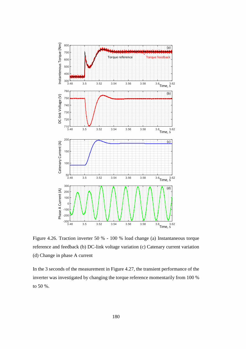
180

Inst

ante

no

us

Torq

ue

(Nm

)

Time, s

DC

-lin

k V

olt

age

(V)

Cat

enar

y C

urr

ent

(A)

Ph

ase

A C

urr

ent

(A)

Time, s

Time, s

Time, s

(a)

(b)

(c)

(d)

Torque feedbackTorque reference



(d) Change in phase A current

In the 3 seconds of the measurement in Figure 4.27, the transient performance of the

inverter was investigated by changing the torque reference momentarily from 100 %

to 50 %.

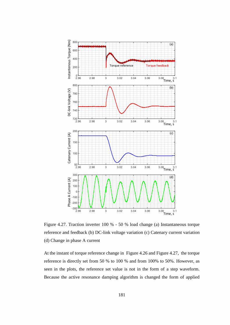
181

Inst

ante

no

us

Torq

ue

(Nm

)

Time, s

DC

-lin

k V

olt

age

(V)

Cat

enar

y C

urr

ent

(A)

Ph

ase

A C

urr

ent

(A)

Time, s

Time, s

Time, s

(a)

(b)

(c)

(d)

Torque feedbackTorque reference



(d) Change in phase A current

At the instant of torque reference change in Figure 4.26 and Figure 4.27, the torque

reference is directly set from 50 % to 100 % and from 100% to 50%. However, as

seen in the plots, the reference set value is not in the form of a step waveform.

Because the active resonance damping algorithm is changed the form of applied

182

torque reference. After the step change occurs in the torque reference, the DC-link

voltage decreases considerably with the effect of the line reactor. At this time, the

active damping algorithm uses the ratio of filtered and unfiltered DC-link voltage as

explained in the control design section, and if there is a sudden decrease in the DC-

link voltage, the torque set value is also decreased automatically from this algorithm.

If there is a sudden increase in DC-link voltage, this time, the set value is increased.

Therefore, the shapes of the torque references and feedbacks differ from the square

wave at the instantaneous reference change.

183

CHAPTER 5

5 FULL-SCALE PHYSICAL SIMULATOR OF ALL SIC TRACTION MOTOR

DRIVE FOR LIGHT RAIL TRANSPORTATION SYSTEMS

It is essential to experimentally validate the simulation results using a real laboratory

setup. A special experimental setup has been built to carry out the experimental

studies. In this chapter, first, the architecture of the experimental test setup is

introduced, and the design aspects of each subsystem component are explained in

detail in this chapter. The experimental results are presented along with figures and

tables in the next chapter.

5.1 Laboratory Experimental Setup

Although the main subject of this study is the design and implementation of a full

SiC-based traction inverter, a full-scale physical simulator per traction motor for all

SiC traction motor drive with an onboard supercapacitor ESS has been developed as

a valuable tool in the design and test of all SiC traction converters [93]. Hence, the

design and implementation of a full SiC-based PWM rectifier and a full SiC Buck-

Boost Converter with a supercapacitor energy storage bank are other important parts

conducted in this work. In addition to this, a motor test bench and a motor drive

system have also been installed in the scope of this study. The complete laboratory

setup in the block diagram form is given in Figure 5.1.

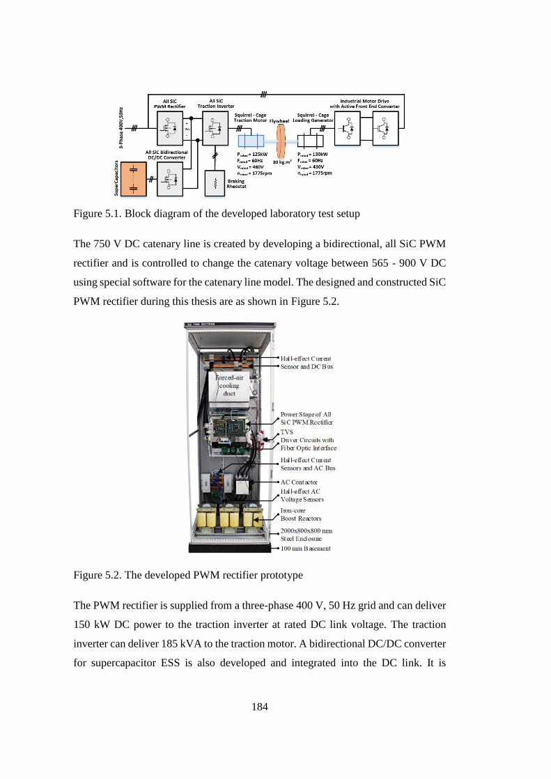
184

Figure 5.1. Block diagram of the developed laboratory test setup

The 750 V DC catenary line is created by developing a bidirectional, all SiC PWM

rectifier and is controlled to change the catenary voltage between 565 - 900 V DC

using special software for the catenary line model. The designed and constructed SiC

PWM rectifier during this thesis are as shown in Figure 5.2.

Figure 5.2. The developed PWM rectifier prototype

The PWM rectifier is supplied from a three-phase 400 V, 50 Hz grid and can deliver

150 kW DC power to the traction inverter at rated DC link voltage. The traction

inverter can deliver 185 kVA to the traction motor. A bidirectional DC/DC converter

for supercapacitor ESS is also developed and integrated into the DC link. It is

185

operated in buck mode during charging and in boost mode during discharging

periods of the supercapacitor bank.

Figure 5.3 shows the all-SiC power MOSFET-based two-level voltage source three-

phase traction inverter developed and implemented in this thesis. Traction inverter

composed of a bottom-to-top mounted power electronic block, current and voltage

sensors, a bulky filter capacitor, forced air cooling duct and fan, air-core line reactor,

soft-start contactor and resistance, and the main line contactor.

Ldc=4mH air-core

Cdc=4.7mH metal-film capacitor

forced air-cooling

duct

gate drivers

current sensors

voltage sensor

Figure 5.3. Full SiC MOSFET based traction inverter prototype

A detailed block diagram of the developed full SiC MOSFET-based traction inverter

is given in Figure 5.4.

Vsens1

idc-

idc+

Cdc_hf

iA

Braking

Resistor

3-ph Squirrel-Cage

Traction MotorS1

Cdc

Ldc

D1 S3 D3 S5 D5

S2 D2 S4 D4 S6 D6 S8 D8

S7 D7

iB

iC

iR

-

+

75

0 V

DC V

sen

s2

1

1

2

3 4

56

7

2

8

9

1 Lem Current Transducer2 Lem Voltage Transducer3 Microelettrica Scientifica Soft Start Contactor4 Reo Soft Start Resistor5 Microelettrica Scientifica Main Lİne Contactor6 Reo Line Inductor7 Elecrtronicon DC-link Capacitor8 Epcos Low ESL DC-link Capacitor9 Cree/Wolfspeed SiC MOSFET Module10 Özdirenç Braking Resistor11 Prodrive Gate Driver

10

11

Figure 5.4. A detailed block diagram of the developed full SiC MOSFET traction

inverter

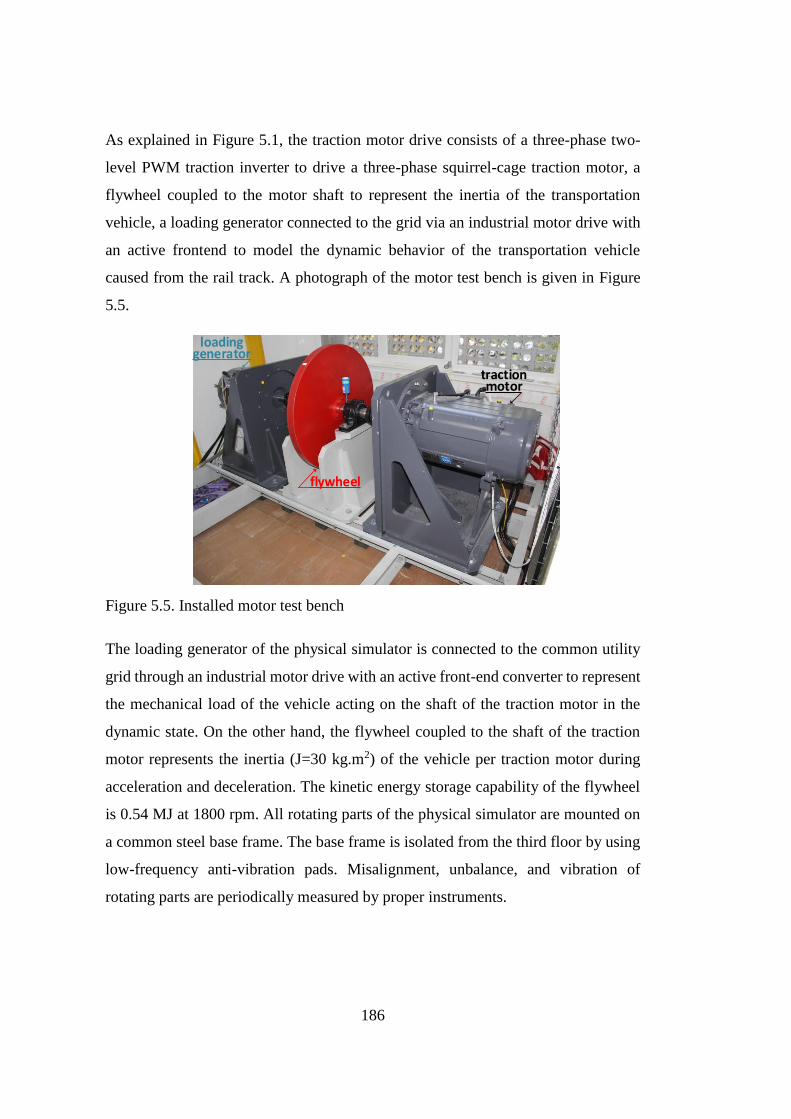
186

As explained in Figure 5.1, the traction motor drive consists of a three-phase two-

level PWM traction inverter to drive a three-phase squirrel-cage traction motor, a

flywheel coupled to the motor shaft to represent the inertia of the transportation

vehicle, a loading generator connected to the grid via an industrial motor drive with

an active frontend to model the dynamic behavior of the transportation vehicle

caused from the rail track. A photograph of the motor test bench is given in Figure

5.5.

traction motor

flywheel

loading generator

Figure 5.5. Installed motor test bench

The loading generator of the physical simulator is connected to the common utility

grid through an industrial motor drive with an active front-end converter to represent

the mechanical load of the vehicle acting on the shaft of the traction motor in the

dynamic state. On the other hand, the flywheel coupled to the shaft of the traction

motor represents the inertia (J=30 kg.m2) of the vehicle per traction motor during

acceleration and deceleration. The kinetic energy storage capability of the flywheel

is 0.54 MJ at 1800 rpm. All rotating parts of the physical simulator are mounted on

a common steel base frame. The base frame is isolated from the third floor by using

low-frequency anti-vibration pads. Misalignment, unbalance, and vibration of

rotating parts are periodically measured by proper instruments.

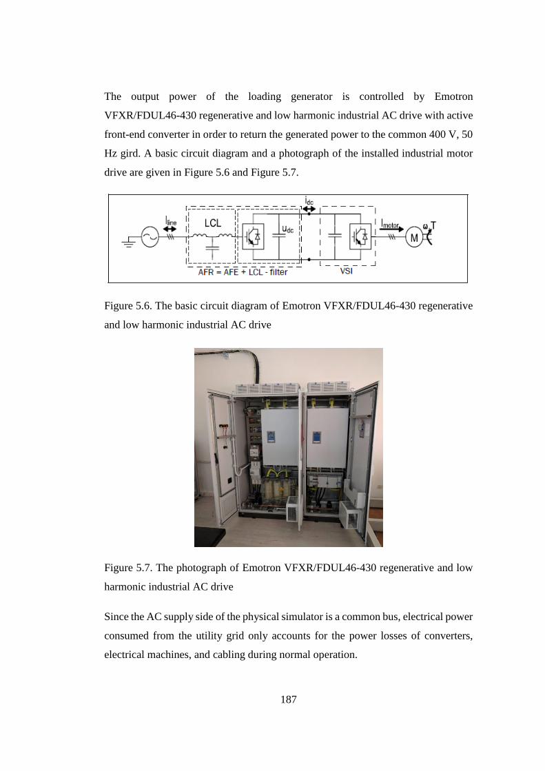
187

The output power of the loading generator is controlled by Emotron

VFXR/FDUL46-430 regenerative and low harmonic industrial AC drive with active

front-end converter in order to return the generated power to the common 400 V, 50

Hz gird. A basic circuit diagram and a photograph of the installed industrial motor

drive are given in Figure 5.6 and Figure 5.7.

Figure 5.6. The basic circuit diagram of Emotron VFXR/FDUL46-430 regenerative

and low harmonic industrial AC drive

Figure 5.7. The photograph of Emotron VFXR/FDUL46-430 regenerative and low

harmonic industrial AC drive

Since the AC supply side of the physical simulator is a common bus, electrical power

consumed from the utility grid only accounts for the power losses of converters,

electrical machines, and cabling during normal operation.

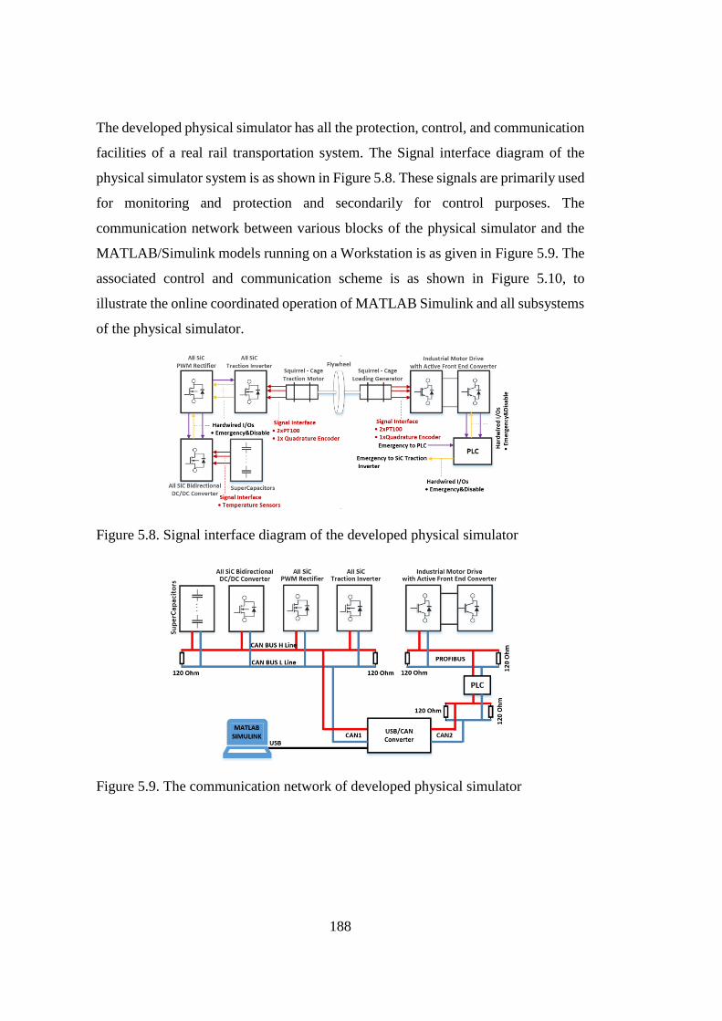
188

The developed physical simulator has all the protection, control, and communication

facilities of a real rail transportation system. The Signal interface diagram of the

physical simulator system is as shown in Figure 5.8. These signals are primarily used

for monitoring and protection and secondarily for control purposes. The

communication network between various blocks of the physical simulator and the

MATLAB/Simulink models running on a Workstation is as given in Figure 5.9. The

associated control and communication scheme is as shown in Figure 5.10, to

illustrate the online coordinated operation of MATLAB Simulink and all subsystems

of the physical simulator.

Figure 5.8. Signal interface diagram of the developed physical simulator

Figure 5.9. The communication network of developed physical simulator

189

Figure 5.10. Control and communication scheme of the developed physical simulator

The footprint of the laboratory test setup is as given in Figure 5.11.

Figure 5.11. The footprint of the test setup 1: 400V, 50 Hz grid panel, 2: PWM

rectifier, 3: Traction inverter 4: Bidirectional buck-boost converter, 5:

Supercapacitor bank, 6: Industrial motor drive, 7: Traction motor&loading

generator, 8: Braking resistor

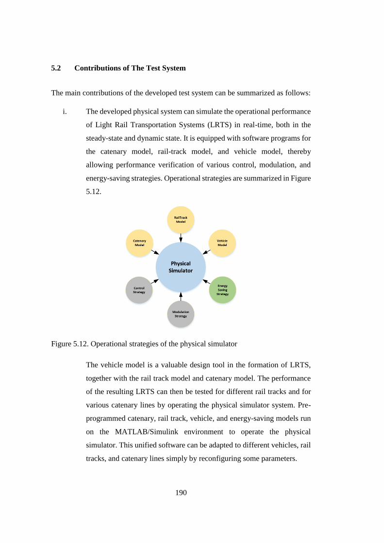
190

5.2 Contributions of The Test System

The main contributions of the developed test system can be summarized as follows:

i. The developed physical system can simulate the operational performance

of Light Rail Transportation Systems (LRTS) in real-time, both in the

steady-state and dynamic state. It is equipped with software programs for

the catenary model, rail-track model, and vehicle model, thereby

allowing performance verification of various control, modulation, and

energy-saving strategies. Operational strategies are summarized in Figure

5.12.

Figure 5.12. Operational strategies of the physical simulator

The vehicle model is a valuable design tool in the formation of LRTS,

together with the rail track model and catenary model. The performance

of the resulting LRTS can then be tested for different rail tracks and for

various catenary lines by operating the physical simulator system. Pre-

programmed catenary, rail track, vehicle, and energy-saving models run

on the MATLAB/Simulink environment to operate the physical

simulator. This unified software can be adapted to different vehicles, rail

tracks, and catenary lines simply by reconfiguring some parameters.

191

ii. The future trend in traction applications is the use of SiC power

MOSFET-based power converters. The physical properties of SiC power

MOSFETs make possible the development of higher efficiency, smaller

size, and weight, and lower current harmonic distortion traction

converters in comparison with the ones based on Si-IGBT. Therefore, the

physical simulator described in this thesis permits the design,

development, and performance testing of all SiC traction converters such

as the traction inverter, PWM rectifier, and ESS.

iii. Since LRTS and its loading system are operating connected to a common

400 V, 50 Hz bus, the physical simulator consumes very low power, i.e.,

nearly 20% of its installed capacity from the utility grid. This permits the

installation of the physical simulator in laboratories that have weak utility

grid connections.

193

CHAPTER 6

6 VERIFICATION OF 500 - 900 VDC, 165 KVA ALL SIC MOSFET BASED

TRACTION INVERTER

In this chapter, the performance of the developed traction system has been presented

using the track data, which is obtained from the real field. The traction inverter is fed

with an active PWM rectifier. The input voltage of the traction inverter is regulated

according to catenary model outputs by utilizing the active PWM rectifier. In order

to load the traction motor, Emotron VFXR/FDUL46-430 regenerative and low

harmonic industrial AC drive is used with another traction motor. A user interface

was also developed and implemented in this study to control Emotron industrial AC

drive. This is carried out using EATON XC-CPU202-EC4M-XV modular PLC. The

vehicle and route model is embedded on the Workstation. In addition to this, the

inverter performance has been tested under various steady-state and dynamic

regimes.

The experimental records have been obtained using the measuring devices listed in

Table 6.1.

Table 6.1 List of The Measuring Devices

- Tektronix MDO3034 Digital Oscilloscope 350 MHz 2.5 Gs/s

- Tektronix P5210 High Voltage Differential Probe 50 MHz

- Tektronix P5205A High Voltage Differential Probe 100 MHz

- Tektronix TCP404XL Current Probe 2 MHz & TCPA400 Current Probe

Amplifier

- CWT Ultra-Miniature High-Frequency Rogowski Current Transducers 30

MHz

- Hioki PW3198 Power Quality Analyzer

- Sper Scientific 800007 2 Channel Thermocouple Measurement Device

194

6.1 Experimental Results

In this section, experimental results taken during this study are illustrated. Before

sharing the measurement results, the accuracy rates of the devices will be presented

in Table 6.2.

Table 6.2 Device Accuracies

Device Oscilloscope Current Probe Voltage Probe

Accuracy ± 1.5 % (AC+DC) ± 1 % (DC), ± 3 % (AC) ± 2 % (AC+DC)

As seen from Table 6.2, the device accuracies are not good enough to take very

sensitive measurements. Additional measuring devices (Yokogawa WT3000 power

analyzer, LEM LV25-1000 voltage transducers and LEM LF-510-S current

transducers with high precision measuring resistance) were used to determine the

calibration coefficients of test setup (oscilloscope, current probe and voltage probe).

Accuries of 0.06 % and 0.1 % were achieved for DC and AC measurements,

respectively. The accuracy of efficicency is calculated as nearly ± 0.32 %.

6.1.1 SiC Power MOSFET Switching Waveforms

Turn-on and turn-off voltage and current waveforms of CAS300M17BM2 SiC

power MOSFETs employed in traction inverter are recorded and given in Figure 6.1

and Figure 6.2. Fall time and rise time of the voltage waveforms are measured as 58

ns and 73 ns, respectively. It is seen that the time durations are very short compared

to the fall and rise times of the Si-IGBTs. The switching time descriptions are defined

using the datasheet of CAS300M17BM2 SiC power MOSFET module.

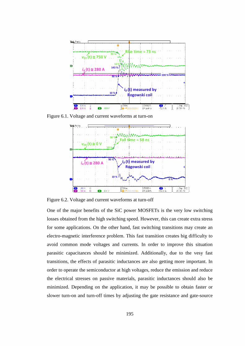
195

iA (t) @ 280 A

vDS (t) @ 750 V

iD (t) measured by Rogowski coil

10 %

90 %

143 %

100 %

90 %

10 %

Rise time = 73 ns

Figure 6.1. Voltage and current waveforms at turn-on

iA (t) @ 280 A iD (t) measured by Rogowski coil

10 %

90 %

0 %

vDS (t) @ 0 V Fall time = 58 ns

10 %

90 %

Figure 6.2. Voltage and current waveforms at turn-off

One of the major benefits of the SiC power MOSFETs is the very low switching

losses obtained from the high switching speed. However, this can create extra stress

for some applications. On the other hand, fast switching transitions may create an

electro-magnetic interference problem. This fast transition creates big difficulty to

avoid common mode voltages and currents. In order to improve this situation

parasitic capacitances should be minimized. Additionally, due to the vesy fast

transitions, the effects of parasitic inductances are also getting more important. In

order to operate the semiconductor at high voltages, reduce the emission and reduce

the electrical stresses on passive materials, parasitic inductances should also be

minimized. Depending on the application, it may be possible to obtain faster or

slower turn-on and turn-off times by adjusting the gate resistance and gate-source

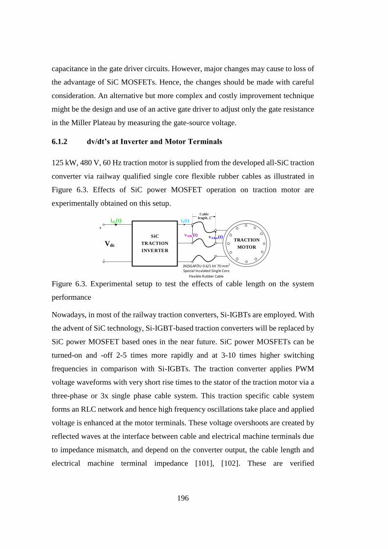
196

capacitance in the gate driver circuits. However, major changes may cause to loss of

the advantage of SiC MOSFETs. Hence, the changes should be made with careful

consideration. An alternative but more complex and costly improvement technique

might be the design and use of an active gate driver to adjust only the gate resistance

in the Miller Plateau by measuring the gate-source voltage.

6.1.2 dv/dt’s at Inverter and Motor Terminals

125 kW, 480 V, 60 Hz traction motor is supplied from the developed all-SiC traction

converter via railway qualified single core flexible rubber cables as illustrated in

Figure 6.3. Effects of SiC power MOSFET operation on traction motor are

experimentally obtained on this setup.

Cable length, lc

vABi (t) SiC

TRACTION

INVERTER

Vdc

+

-

idc(t) iA(t)

vABm(t)TRACTION

MOTOR

(N)SGAFÖU 0.6/1 kV 70 mm2 Special Insulated Single Core

Flexible Rubber Cable Figure 6.3. Experimental setup to test the effects of cable length on the system

performance

Nowadays, in most of the railway traction converters, Si-IGBTs are employed. With

the advent of SiC technology, Si-IGBT-based traction converters will be replaced by

SiC power MOSFET based ones in the near future. SiC power MOSFETs can be

turned-on and -off 2-5 times more rapidly and at 3-10 times higher switching

frequencies in comparison with Si-IGBTs. The traction converter applies PWM

voltage waveforms with very short rise times to the stator of the traction motor via a

three-phase or 3x single phase cable system. This traction specific cable system

forms an RLC network and hence high frequency oscillations take place and applied

voltage is enhanced at the motor terminals. These voltage overshoots are created by

reflected waves at the interface between cable and electrical machine terminals due

to impedance mismatch, and depend on the converter output, the cable length and

electrical machine terminal impedance [101], [102]. These are verified

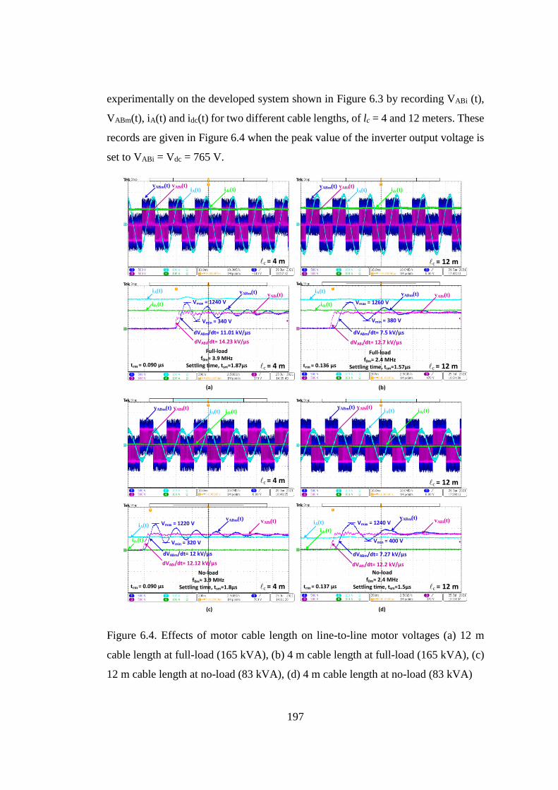
197

experimentally on the developed system shown in Figure 6.3 by recording VABi (t),

VABm(t), iA(t) and idc(t) for two different cable lengths, of lc = 4 and 12 meters. These

records are given in Figure 6.4 when the peak value of the inverter output voltage is

set to VABi = Vdc = 765 V.

vABm(t) vABi(t)

iA(t) idc(t)

lc = 12 m

vABm(t) vABi(t)

iA(t) idc(t)

lc = 4 m

(a)

dVABm/dt= 11.01 kV/µs

dVABi/dt= 14.23 kV/µs

Full-loadf0m 3.9 MHz

Settling time, tsm=1.87µs

Vmax = 1240 V

Vmin = 340 V

vABm(t)vABi(t)

iA(t)

idc(t)

lc = 4 mtrm = 0.090 µs

vABm(t) vABi(t)

iA(t) idc(t)

lc = 12 m

vABm(t) vABi(t)

iA(t) idc(t)

lc = 4 m

(c)

dVABm/dt= 12 kV/µs


No-loadf0m 3.9 MHz


Vmax = 1220 V

Vmin = 320 V

vABm(t) vABi(t)

iA(t)

idc(t)

lc = 4 mtrm = 0.090 µs

(b)





Vmax = 1260 V

Vmin = 380 V

vABm(t) vABi(t)

iA(t)

idc(t)

lc = 12 mtrm = 0.136 µs

(d)



No-loadf0m 2.4 MHz


Vmax = 1240 V

Vmin = 400 V

vABm(t)vABi(t) iA(t)

idc(t)

lc = 12 mtrm = 0.137 µs

Figure 6.4. Effects of motor cable length on line-to-line motor voltages (a) 12 m

cable length at full-load (165 kVA), (b) 4 m cable length at full-load (165 kVA), (c)

12 m cable length at no-load (83 kVA), (d) 4 m cable length at no-load (83 kVA)

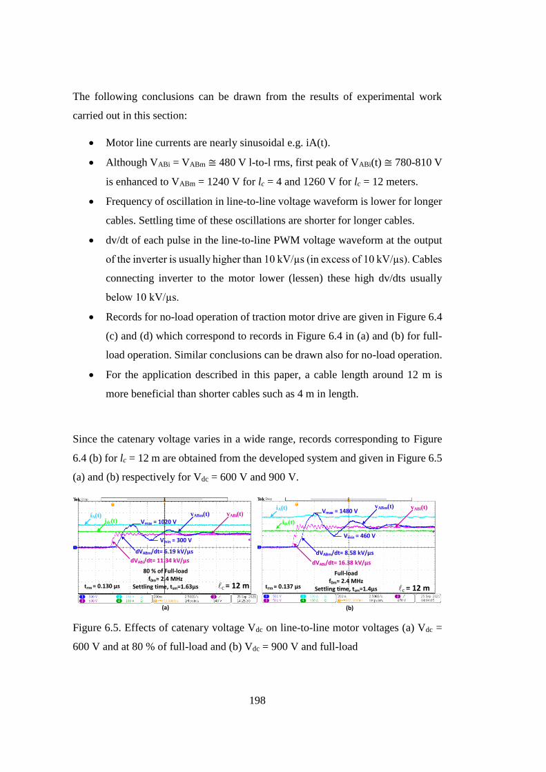
198

The following conclusions can be drawn from the results of experimental work

carried out in this section:

Motor line currents are nearly sinusoidal e.g. iA(t).

Although VABi = VABm ≅ 480 V l-to-l rms, first peak of VABi(t) ≅ 780-810 V

is enhanced to VABm = 1240 V for lc = 4 and 1260 V for lc = 12 meters.

Frequency of oscillation in line-to-line voltage waveform is lower for longer

cables. Settling time of these oscillations are shorter for longer cables.

dv/dt of each pulse in the line-to-line PWM voltage waveform at the output

of the inverter is usually higher than 10 kV/µs (in excess of 10 kV/µs). Cables

connecting inverter to the motor lower (lessen) these high dv/dts usually

below 10 kV/µs.

Records for no-load operation of traction motor drive are given in Figure 6.4

(c) and (d) which correspond to records in Figure 6.4 in (a) and (b) for full-

load operation. Similar conclusions can be drawn also for no-load operation.

For the application described in this paper, a cable length around 12 m is

more beneficial than shorter cables such as 4 m in length.

Since the catenary voltage varies in a wide range, records corresponding to Figure

6.4 (b) for lc = 12 m are obtained from the developed system and given in Figure 6.5

(a) and (b) respectively for Vdc = 600 V and 900 V.



80 % of Full-loadf0m 2.4 MHz


Vmax = 1020 V

Vmin = 300 V

vABm(t) vABi(t) iA(t)idc(t)

lc = 12 mtrm = 0.130 µs

(a)





Vmax = 1480 V

Vmin = 460 V

vABm(t) vABi(t) iA(t)

idc(t)

lc = 12 mtrm = 0.137 µs

(b)

Figure 6.5. Effects of catenary voltage Vdc on line-to-line motor voltages (a) Vdc =

600 V and at 80 % of full-load and (b) Vdc = 900 V and full-load

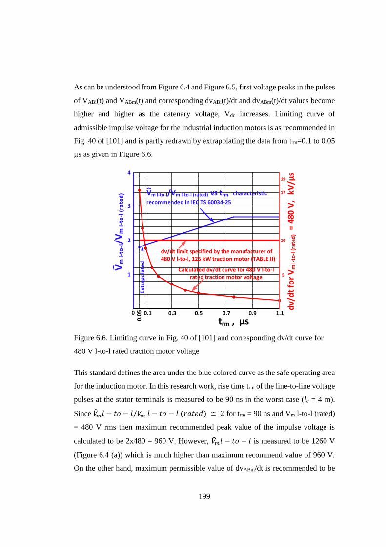
199

As can be understood from Figure 6.4 and Figure 6.5, first voltage peaks in the pulses

of VABi(t) and VABm(t) and corresponding dvABi(t)/dt and dvABm(t)/dt values become

higher and higher as the catenary voltage, Vdc increases. Limiting curve of

admissible impulse voltage for the industrial induction motors is as recommended in

Fig. 40 of [101] and is partly redrawn by extrapolating the data from trm=0.1 to 0.05

µs as given in Figure 6.6.

17

5

0.0

5 0.1 0.3

dv/

dt

for

Vm

l-to

-l (

rate

d)

= 4

80 V

, k

V/µ

s

1

2

3

4

10

19

0.5 0.7 0.9 1.1

trm , µs0

Calculated dv/dt curve for 480 V l-to-l rated traction motor voltage

dv/dt limit specified by the manufacturer of 480 V l-to-l, 125 kW traction motor (TABLE II)

Ext

rap

ola

ted

Vm

l-to

-l/V

m l-

to-l

(ra

ted

) Vm l-to-l/Vm l-to-l (rated) vs trm characteristic

recommended in IEC TS 60034-25

Figure 6.6. Limiting curve in Fig. 40 of [101] and corresponding dv/dt curve for

480 V l-to-l rated traction motor voltage

This standard defines the area under the blue colored curve as the safe operating area

for the induction motor. In this research work, rise time trm of the line-to-line voltage

pulses at the stator terminals is measured to be 90 ns in the worst case (lc = 4 m).

Since �̂�𝑚𝑙 − 𝑡𝑜 − 𝑙/𝑉𝑚 𝑙 − 𝑡𝑜 − 𝑙 (𝑟𝑎𝑡𝑒𝑑) ≅ 2 for trm = 90 ns and Vm l-to-l (rated)

= 480 V rms then maximum recommended peak value of the impulse voltage is

calculated to be 2x480 = 960 V. However, �̂�𝑚𝑙 − 𝑡𝑜 − 𝑙 is measured to be 1260 V

(Figure 6.4 (a)) which is much higher than maximum recommend value of 960 V.

On the other hand, maximum permissible value of dvABm/dt is recommended to be

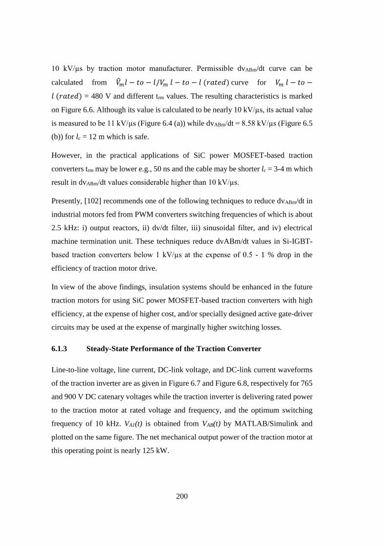
200

10 kV/µs by traction motor manufacturer. Permissible dvABm/dt curve can be

calculated from �̂�𝑚𝑙 − 𝑡𝑜 − 𝑙/𝑉𝑚 𝑙 − 𝑡𝑜 − 𝑙 (𝑟𝑎𝑡𝑒𝑑) curve for 𝑉𝑚 𝑙 − 𝑡𝑜 −

𝑙 (𝑟𝑎𝑡𝑒𝑑) = 480 V and different trm values. The resulting characteristics is marked

on Figure 6.6. Although its value is calculated to be nearly 10 kV/µs, its actual value

is measured to be 11 kV/µs (Figure 6.4 (a)) while dvABm/dt = 8.58 kV/µs (Figure 6.5

(b)) for lc = 12 m which is safe.

However, in the practical applications of SiC power MOSFET-based traction

converters trm may be lower e.g., 50 ns and the cable may be shorter lc = 3-4 m which

result in dvABm/dt values considerable higher than 10 kV/µs.

Presently, [102] recommends one of the following techniques to reduce dvABm/dt in

industrial motors fed from PWM converters switching frequencies of which is about

2.5 kHz: i) output reactors, ii) dv/dt filter, iii) sinusoidal filter, and iv) electrical

machine termination unit. These techniques reduce dvABm/dt values in Si-IGBT-

based traction converters below 1 kV/µs at the expense of 0.5 - 1 % drop in the

efficiency of traction motor drive.

In view of the above findings, insulation systems should be enhanced in the future

traction motors for using SiC power MOSFET-based traction converters with high

efficiency, at the expense of higher cost, and/or specially designed active gate-driver

circuits may be used at the expense of marginally higher switching losses.

6.1.3 Steady-State Performance of the Traction Converter

Line-to-line voltage, line current, DC-link voltage, and DC-link current waveforms

of the traction inverter are as given in Figure 6.7 and Figure 6.8, respectively for 765

and 900 V DC catenary voltages while the traction inverter is delivering rated power

to the traction motor at rated voltage and frequency, and the optimum switching

frequency of 10 kHz. VA1(t) is obtained from VAB(t) by MATLAB/Simulink and

plotted on the same figure. The net mechanical output power of the traction motor at

this operating point is nearly 125 kW.

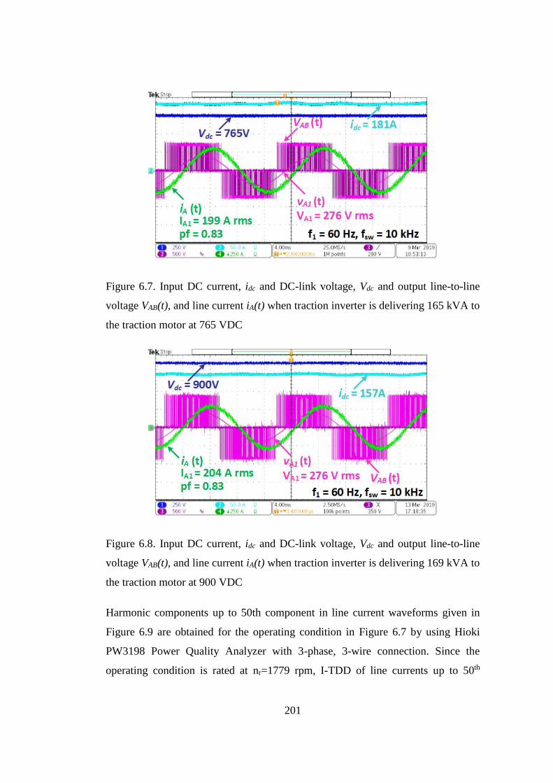
201



the traction motor at 765 VDC



the traction motor at 900 VDC

Harmonic components up to 50th component in line current waveforms given in

Figure 6.9 are obtained for the operating condition in Figure 6.7 by using Hioki

PW3198 Power Quality Analyzer with 3-phase, 3-wire connection. Since the

operating condition is rated at nr=1779 rpm, I-TDD of line currents up to 50th

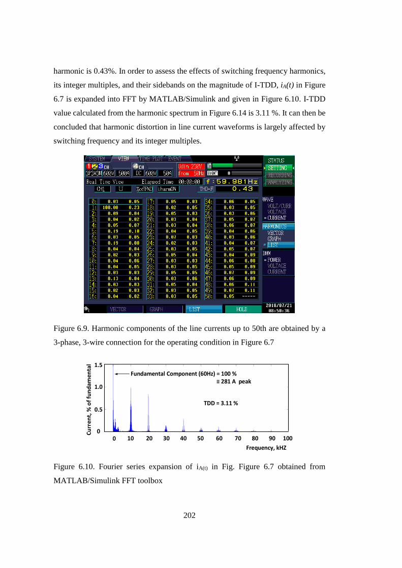
202

harmonic is 0.43%. In order to assess the effects of switching frequency harmonics,

its integer multiples, and their sidebands on the magnitude of I-TDD, iA(t) in Figure

6.7 is expanded into FFT by MATLAB/Simulink and given in Figure 6.10. I-TDD

value calculated from the harmonic spectrum in Figure 6.14 is 3.11 %. It can then be

concluded that harmonic distortion in line current waveforms is largely affected by

switching frequency and its integer multiples.

Figure 6.9. Harmonic components of the line currents up to 50th are obtained by a

3-phase, 3-wire connection for the operating condition in Figure 6.7

Fundamental Component (60Hz) = 100 % 281 A peak

Cu

rre

nt,

% o

f fu

nd

am

en

tal

TDD = 3.11 %

Frequency, kHZ

200 40 60 80 10010 5030 70 900

0.5

1.0

1.5

Figure 6.10. Fourier series expansion of iA(t) in Fig. Figure 6.7 obtained from

MATLAB/Simulink FFT toolbox

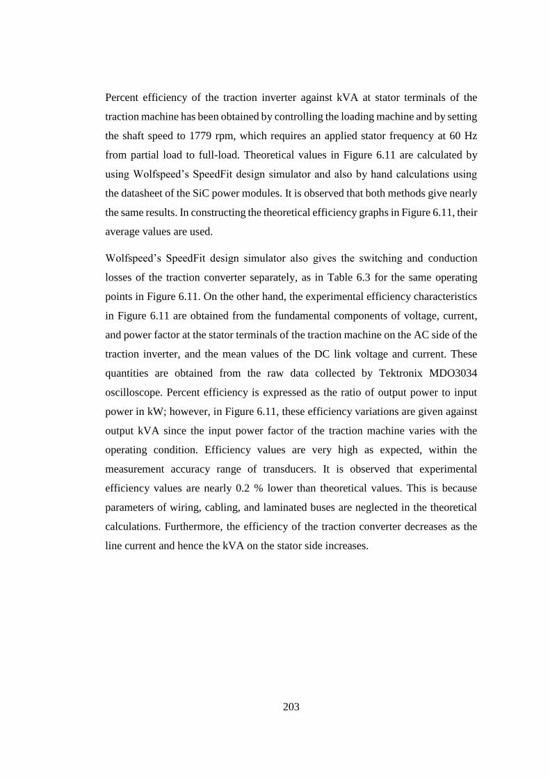
203

Percent efficiency of the traction inverter against kVA at stator terminals of the

traction machine has been obtained by controlling the loading machine and by setting

the shaft speed to 1779 rpm, which requires an applied stator frequency at 60 Hz

from partial load to full-load. Theoretical values in Figure 6.11 are calculated by

using Wolfspeed’s SpeedFit design simulator and also by hand calculations using

the datasheet of the SiC power modules. It is observed that both methods give nearly

the same results. In constructing the theoretical efficiency graphs in Figure 6.11, their

average values are used.

Wolfspeed’s SpeedFit design simulator also gives the switching and conduction

losses of the traction converter separately, as in Table 6.3 for the same operating

points in Figure 6.11. On the other hand, the experimental efficiency characteristics

in Figure 6.11 are obtained from the fundamental components of voltage, current,

and power factor at the stator terminals of the traction machine on the AC side of the

traction inverter, and the mean values of the DC link voltage and current. These

quantities are obtained from the raw data collected by Tektronix MDO3034

oscilloscope. Percent efficiency is expressed as the ratio of output power to input

power in kW; however, in Figure 6.11, these efficiency variations are given against

output kVA since the input power factor of the traction machine varies with the

operating condition. Efficiency values are very high as expected, within the

measurement accuracy range of transducers. It is observed that experimental

efficiency values are nearly 0.2 % lower than theoretical values. This is because

parameters of wiring, cabling, and laminated buses are neglected in the theoretical

calculations. Furthermore, the efficiency of the traction converter decreases as the

line current and hence the kVA on the stator side increases.

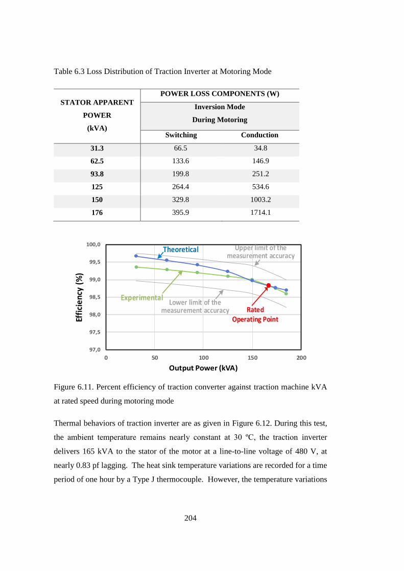
204

Table 6.3 Loss Distribution of Traction Inverter at Motoring Mode

STATOR APPARENT

POWER

(kVA)

POWER LOSS COMPONENTS (W)

Inversion Mode

During Motoring

Switching Conduction

31.3 66.5 34.8

62.5 133.6 146.9

93.8 199.8 251.2

125 264.4 534.6

150 329.8 1003.2

176 395.9 1714.1

97,0

97,5

98,0

98,5

99,0

99,5

100,0

0 50 100 150 200

Effi

cien

cy (

%)

Output Power (kVA)

Theoretical

Experimental

Upper limit of the measurement accuracy

Lower limit of the measurement accuracy Rated

Operating Point


at rated speed during motoring mode

Thermal behaviors of traction inverter are as given in Figure 6.12. During this test,

the ambient temperature remains nearly constant at 30 ºC, the traction inverter

delivers 165 kVA to the stator of the motor at a line-to-line voltage of 480 V, at

nearly 0.83 pf lagging. The heat sink temperature variations are recorded for a time

period of one hour by a Type J thermocouple. However, the temperature variations

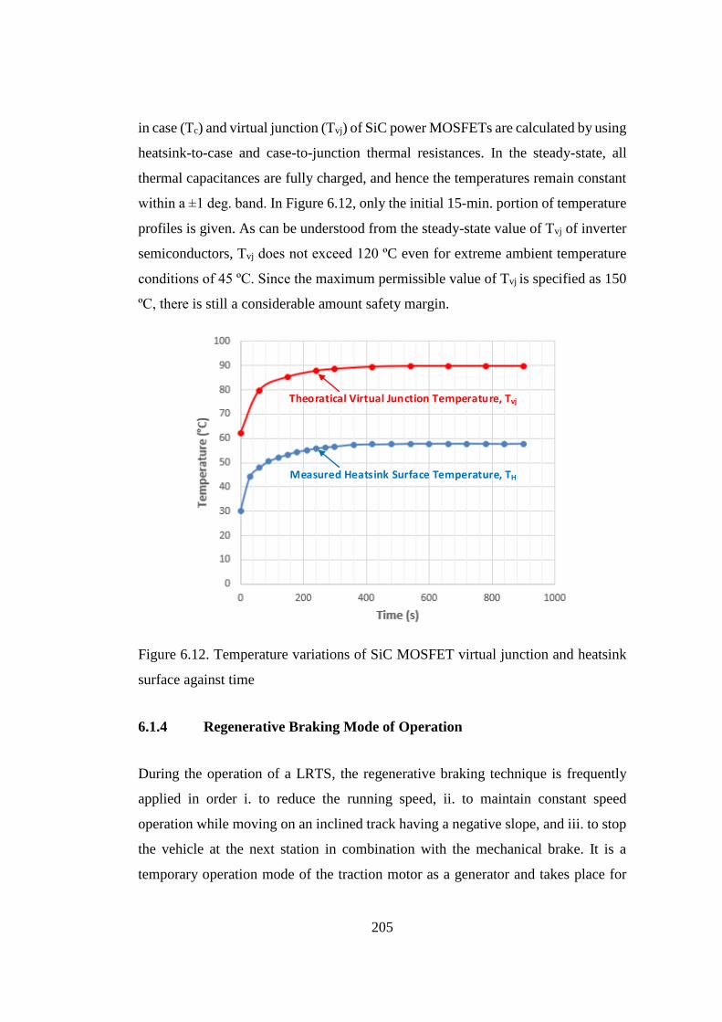
205

in case (Tc) and virtual junction (Tvj) of SiC power MOSFETs are calculated by using

heatsink-to-case and case-to-junction thermal resistances. In the steady-state, all

thermal capacitances are fully charged, and hence the temperatures remain constant

within a ±1 deg. band. In Figure 6.12, only the initial 15-min. portion of temperature

profiles is given. As can be understood from the steady-state value of Tvj of inverter

semiconductors, Tvj does not exceed 120 ºC even for extreme ambient temperature

conditions of 45 ºC. Since the maximum permissible value of Tvj is specified as 150

ºC, there is still a considerable amount safety margin.

Theoratical Virtual Junction Temperature, Tvj

Measured Heatsink Surface Temperature, TH

Figure 6.12. Temperature variations of SiC MOSFET virtual junction and heatsink

surface against time

6.1.4 Regenerative Braking Mode of Operation

During the operation of a LRTS, the regenerative braking technique is frequently

applied in order i. to reduce the running speed, ii. to maintain constant speed

operation while moving on an inclined track having a negative slope, and iii. to stop

the vehicle at the next station in combination with the mechanical brake. It is a

temporary operation mode of the traction motor as a generator and takes place for

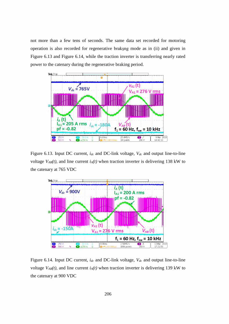
206

not more than a few tens of seconds. The same data set recorded for motoring

operation is also recorded for regenerative brakşng mode as in (ii) and given in

Figure 6.13 and Figure 6.14, while the traction inverter is transferring nearly rated

power to the catenary during the regenerative braking period.



the catenary at 765 VDC



the catenary at 900 VDC

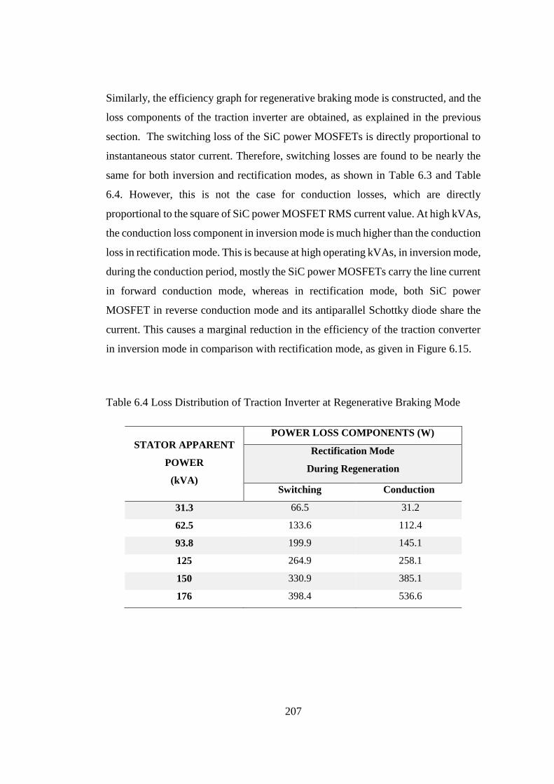
207

Similarly, the efficiency graph for regenerative braking mode is constructed, and the

loss components of the traction inverter are obtained, as explained in the previous

section. The switching loss of the SiC power MOSFETs is directly proportional to

instantaneous stator current. Therefore, switching losses are found to be nearly the

same for both inversion and rectification modes, as shown in Table 6.3 and Table

6.4. However, this is not the case for conduction losses, which are directly

proportional to the square of SiC power MOSFET RMS current value. At high kVAs,

the conduction loss component in inversion mode is much higher than the conduction

loss in rectification mode. This is because at high operating kVAs, in inversion mode,

during the conduction period, mostly the SiC power MOSFETs carry the line current

in forward conduction mode, whereas in rectification mode, both SiC power

MOSFET in reverse conduction mode and its antiparallel Schottky diode share the

current. This causes a marginal reduction in the efficiency of the traction converter

in inversion mode in comparison with rectification mode, as given in Figure 6.15.

Table 6.4 Loss Distribution of Traction Inverter at Regenerative Braking Mode

STATOR APPARENT

POWER

(kVA)

POWER LOSS COMPONENTS (W)

Rectification Mode

During Regeneration

Switching Conduction

31.3 66.5 31.2

62.5 133.6 112.4

93.8 199.9 145.1

125 264.9 258.1

150 330.9 385.1

176 398.4 536.6

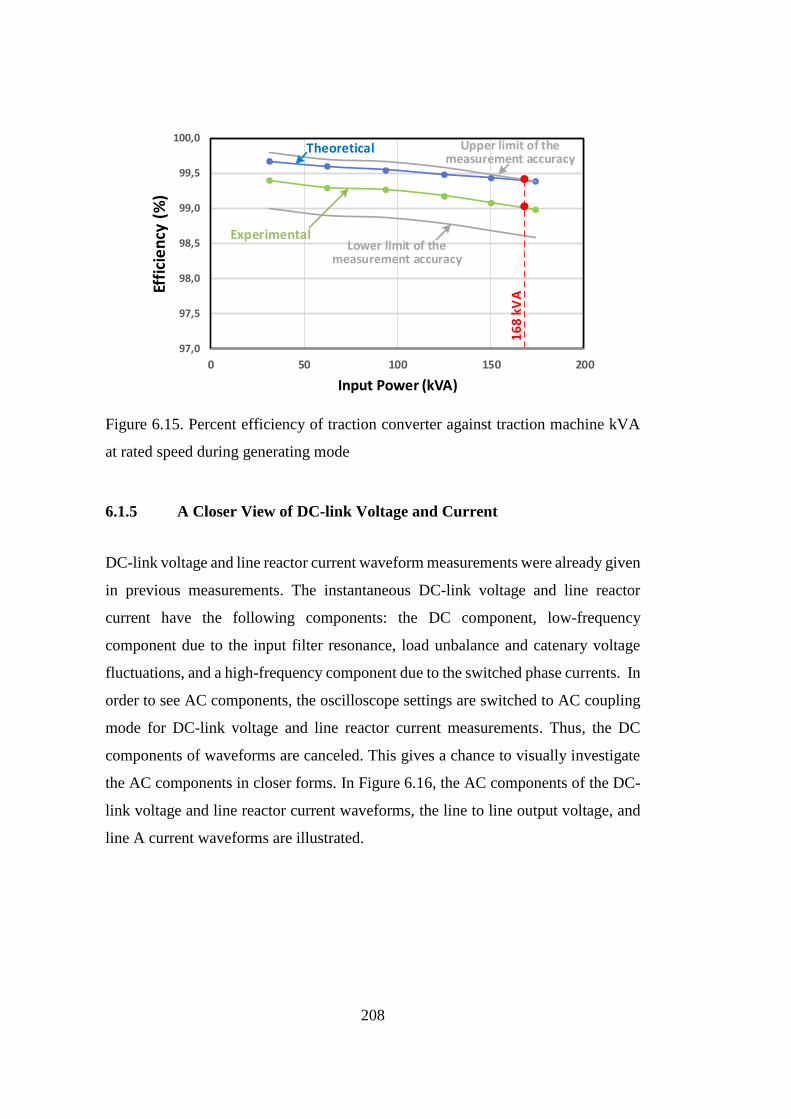
208

97,0

97,5

98,0

98,5

99,0

99,5

100,0

0 50 100 150 200

Effi

cie

ncy

(%

)

Input Power (kVA)

16

8 kV

A

Theoretical Upper limit of the measurement accuracy

ExperimentalLower limit of the

measurement accuracy


at rated speed during generating mode

6.1.5 A Closer View of DC-link Voltage and Current

DC-link voltage and line reactor current waveform measurements were already given

in previous measurements. The instantaneous DC-link voltage and line reactor

current have the following components: the DC component, low-frequency

component due to the input filter resonance, load unbalance and catenary voltage

fluctuations, and a high-frequency component due to the switched phase currents. In

order to see AC components, the oscilloscope settings are switched to AC coupling

mode for DC-link voltage and line reactor current measurements. Thus, the DC

components of waveforms are canceled. This gives a chance to visually investigate

the AC components in closer forms. In Figure 6.16, the AC components of the DC-

link voltage and line reactor current waveforms, the line to line output voltage, and

line A current waveforms are illustrated.

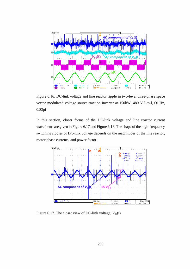
209

AC component of Vdc(t)

AC component of Vdc(t)VAB(t)

iA(t)

Figure 6.16. DC-link voltage and line reactor ripple in two-level three-phase space

vector modulated voltage source traction inverter at 150kW, 480 V l-to-l, 60 Hz,

0.83pf

In this section, closer forms of the DC-link voltage and line reactor current

waveforms are given in Figure 6.17 and Figure 6.18. The shape of the high-frequency

switching ripples of DC-link voltage depends on the magnitudes of the line reactor,

motor phase currents, and power factor.

AC component of Vdc(t) 15 Vp-p

Figure 6.17. The closer view of DC-link voltage, Vdc(t)

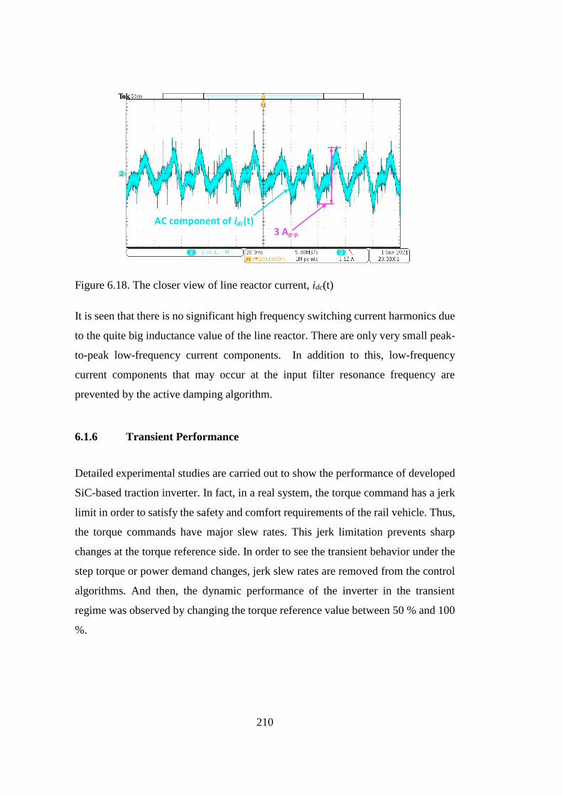
210

AC component of idc(t)3 Ap-p

Figure 6.18. The closer view of line reactor current, idc(t)

It is seen that there is no significant high frequency switching current harmonics due

to the quite big inductance value of the line reactor. There are only very small peak-

to-peak low-frequency current components. In addition to this, low-frequency

current components that may occur at the input filter resonance frequency are

prevented by the active damping algorithm.

6.1.6 Transient Performance

Detailed experimental studies are carried out to show the performance of developed

SiC-based traction inverter. In fact, in a real system, the torque command has a jerk

limit in order to satisfy the safety and comfort requirements of the rail vehicle. Thus,

the torque commands have major slew rates. This jerk limitation prevents sharp

changes at the torque reference side. In order to see the transient behavior under the

step torque or power demand changes, jerk slew rates are removed from the control

algorithms. And then, the dynamic performance of the inverter in the transient

regime was observed by changing the torque reference value between 50 % and 100

%.

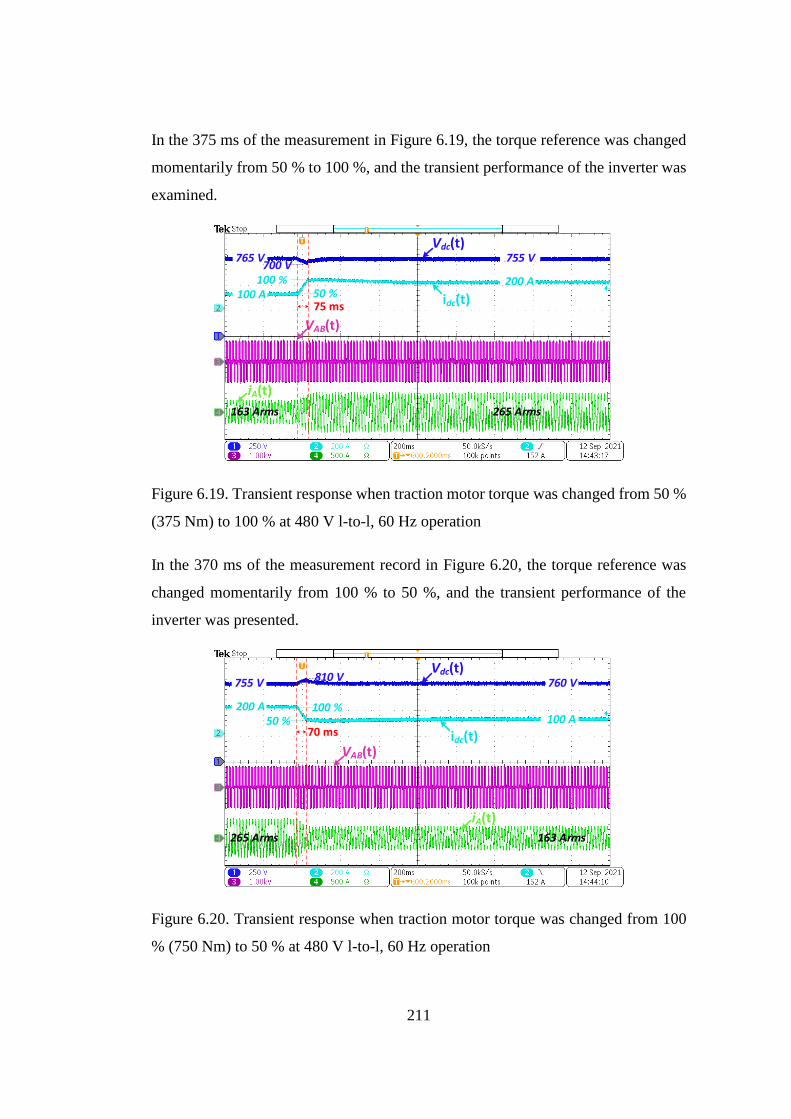
211

In the 375 ms of the measurement in Figure 6.19, the torque reference was changed

momentarily from 50 % to 100 %, and the transient performance of the inverter was

examined.

Vdc(t)

idc(t)

VAB(t)

iA(t)

75 ms 50 %

100 % 100 A

200 A

765 V 755 V700 V

163 Arms 265 Arms

Figure 6.19. Transient response when traction motor torque was changed from 50 %

(375 Nm) to 100 % at 480 V l-to-l, 60 Hz operation

In the 370 ms of the measurement record in Figure 6.20, the torque reference was

changed momentarily from 100 % to 50 %, and the transient performance of the

inverter was presented.

Vdc(t)

idc(t)VAB(t)

iA(t)

70 ms 50 %

100 % 200 A 100 A

755 V 760 V810 V

265 Arms 163 Arms

Figure 6.20. Transient response when traction motor torque was changed from 100

% (750 Nm) to 50 % at 480 V l-to-l, 60 Hz operation

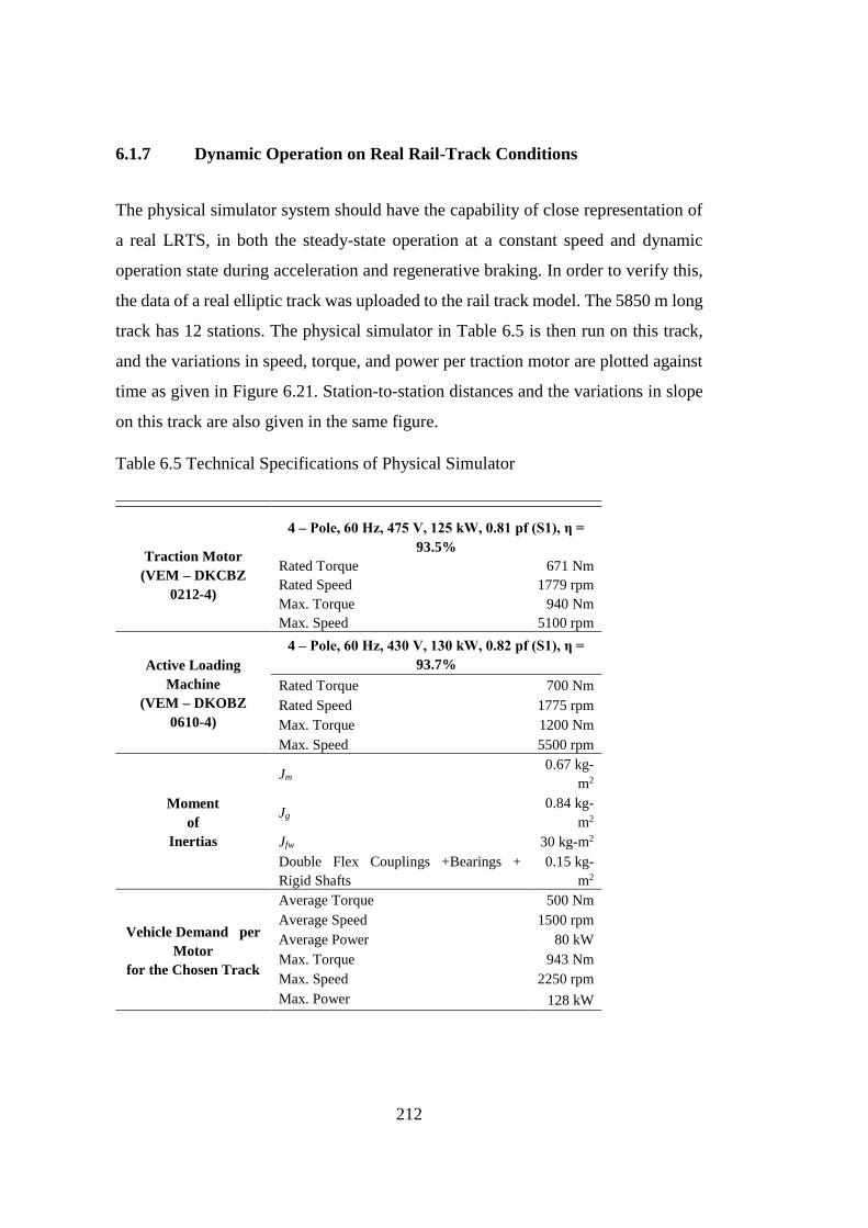
212

6.1.7 Dynamic Operation on Real Rail-Track Conditions

The physical simulator system should have the capability of close representation of

a real LRTS, in both the steady-state operation at a constant speed and dynamic

operation state during acceleration and regenerative braking. In order to verify this,

the data of a real elliptic track was uploaded to the rail track model. The 5850 m long

track has 12 stations. The physical simulator in Table 6.5 is then run on this track,

and the variations in speed, torque, and power per traction motor are plotted against

time as given in Figure 6.21. Station-to-station distances and the variations in slope

on this track are also given in the same figure.

Table 6.5 Technical Specifications of Physical Simulator

Traction Motor

(VEM – DKCBZ

0212-4)

4 – Pole, 60 Hz, 475 V, 125 kW, 0.81 pf (S1), η =

93.5%

Rated Torque 671 Nm


Max. Torque 940 Nm

Max. Speed 5100 rpm

Active Loading

Machine

(VEM – DKOBZ

0610-4)

4 – Pole, 60 Hz, 430 V, 130 kW, 0.82 pf (S1), η =

93.7%

Rated Torque 700 Nm


Max. Torque 1200 Nm

Max. Speed 5500 rpm

Moment

of

Inertias

Jm 0.67 kg-

m2

Jg 0.84 kg-

m2

Jfw 30 kg-m2

Double Flex Couplings +Bearings +

Rigid Shafts

0.15 kg-

m2

Vehicle Demand per

Motor

for the Chosen Track

Average Torque 500 Nm

Average Speed 1500 rpm

Average Power 80 kW

Max. Torque 943 Nm

Max. Speed 2250 rpm

Max. Power 128 kW

213

Figure 6.21. Records of the physical simulator in Table 6.5 while the light rail vehicle

is running on a real elliptic track

In order to test the performance of the traction system developed in this thesis and

hence the vehicle body structure formed as in Table 3.1, on real rail-track conditions,

the physical simulator per traction motor is operated for several running conditions.

Among these, records corresponding to acceleration and deceleration on a level

track, acceleration on a maximum positive slope and, regenerative braking on a

maximum negative slope are plotted.

The first test consists of the acceleration, constant speed operation, and deceleration

instants on a level track, and the results are illustrated in Figure 6.22. In Figure 6.22

(a), traction motor shaft speed, traction motor shaft torque, and load motor torque

variations against time are plotted, while one phase current of traction motor is

exhibited in Figure 6.22 (b).

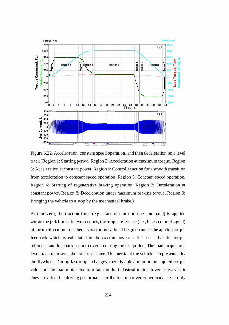
214

0

250

500

750

1000

-250

Mo

tor

Torq

ue

, Tm

Torq

ue

Co

mm

and

, Tre

f

-500

Load

To

rqu

e, T

r/m

Ro

tati

on

al S

pee

d, n

r

-750

-1000

1250

Speed, rpm

0

500

1500

2000

-500

1000

-1000

-1500

-2000

2500

Torque, NmLi

ne

Cu

rren

t, I A

Region 2 Region 4 Region 5 Region 8

Reg

ion

3

Reg

ion

1

Reg

ion

6

Reg

ion

7

Reg

ion

9

0

400

800

-400

-800

200

600

-200

-600

0 2 4 6 8 10 12 14 16 18 20 22 24 26 28 30 32 34 36 38 40Time, s

(a)

(b)

Figure 6.22. Acceleration, constant speed operation, and then deceleration on a level

track (Region 1: Starting period, Region 2: Acceleration at maximum torque, Region

3: Acceleration at constant power, Region 4: Controller action for a smooth transition

from acceleration to constant speed operation, Region 5: Constant speed operation,

Region 6: Starting of regenerative braking operation, Region 7: Deceleration at

constant power, Region 8: Deceleration under maximum braking torque, Region 9:

Bringing the vehicle to a stop by the mechanical brake.)

At time zero, the traction force (e.g., traction motor torque command) is applied

within the jerk limits. In two seconds, the torque reference (i.e., black colored signal)

of the traction motor reached its maximum value. The green one is the applied torque

feedback which is calculated in the traction inverter. It is seen that the torque

reference and feedback seem to overlap during the test period. The load torque on a

level track represents the train resistance. The inertia of the vehicle is represented by

the flywheel. During fast torque changes, there is a deviation in the applied torque

values of the load motor due to a fault in the industrial motor driver. However, it

does not affect the driving performance or the traction inverter performance. It only

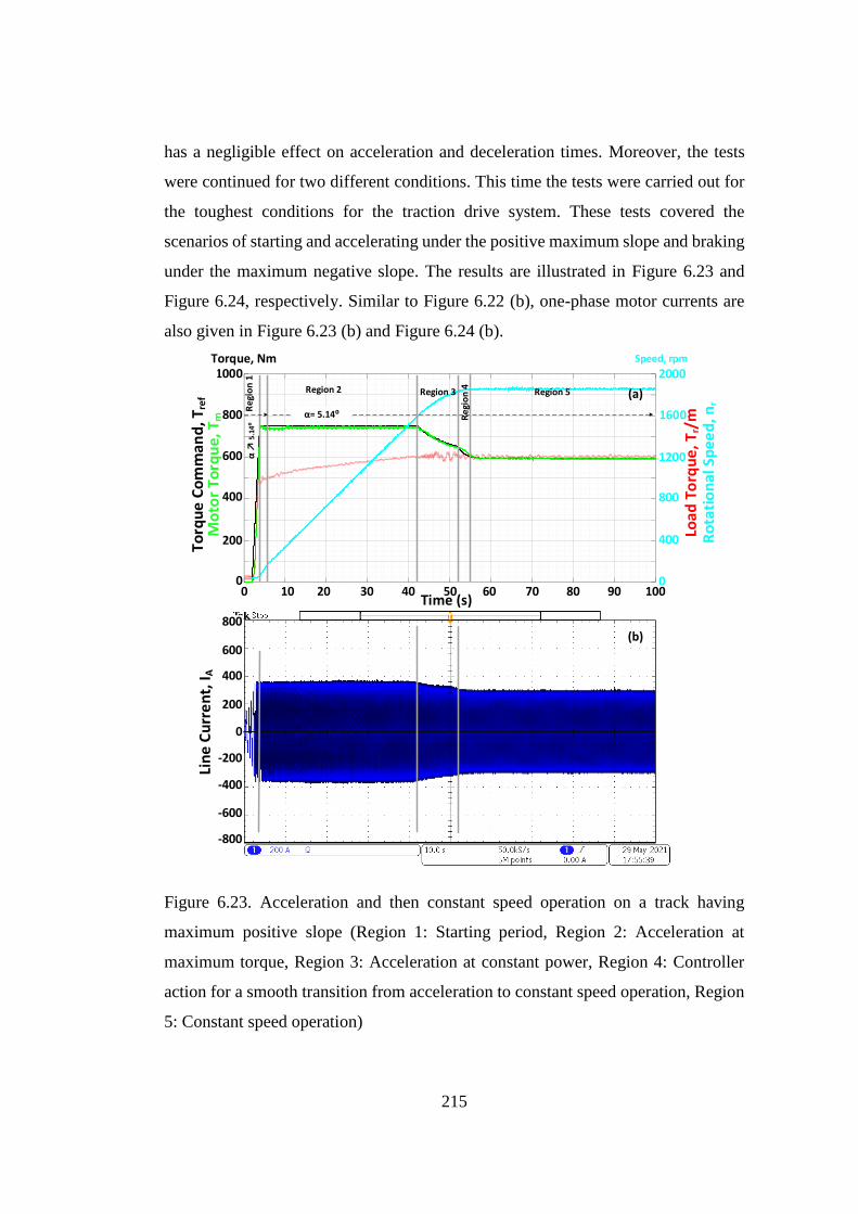
215

has a negligible effect on acceleration and deceleration times. Moreover, the tests

were continued for two different conditions. This time the tests were carried out for

the toughest conditions for the traction drive system. These tests covered the

scenarios of starting and accelerating under the positive maximum slope and braking

under the maximum negative slope. The results are illustrated in Figure 6.23 and

Figure 6.24, respectively. Similar to Figure 6.22 (b), one-phase motor currents are

also given in Figure 6.23 (b) and Figure 6.24 (b).

0

400

600

800

1000

200

Mo

tor

To

rqu

e, T

m

Time (s)0 10 20 30 40 50 60 70 80 90 100

0

800

1200

1600

2000

400

To

rqu

e C

om

ma

nd

, Tre

f

Loa

d T

orq

ue

, Tr/

mR

ota

tio

na

l Sp

ee

d, n

r

α= 5.14⁰

α

5.1

4⁰

Region 2

Re

gio

n 1

Region 3 Region 5

Lin

e C

urr

en

t, I

A

0

400

800

-400

-800

-600

-200

200

600

Torque, Nm Speed, rpm

Re

gio

n 4 (a)

(b)

Figure 6.23. Acceleration and then constant speed operation on a track having

maximum positive slope (Region 1: Starting period, Region 2: Acceleration at

maximum torque, Region 3: Acceleration at constant power, Region 4: Controller

action for a smooth transition from acceleration to constant speed operation, Region

5: Constant speed operation)

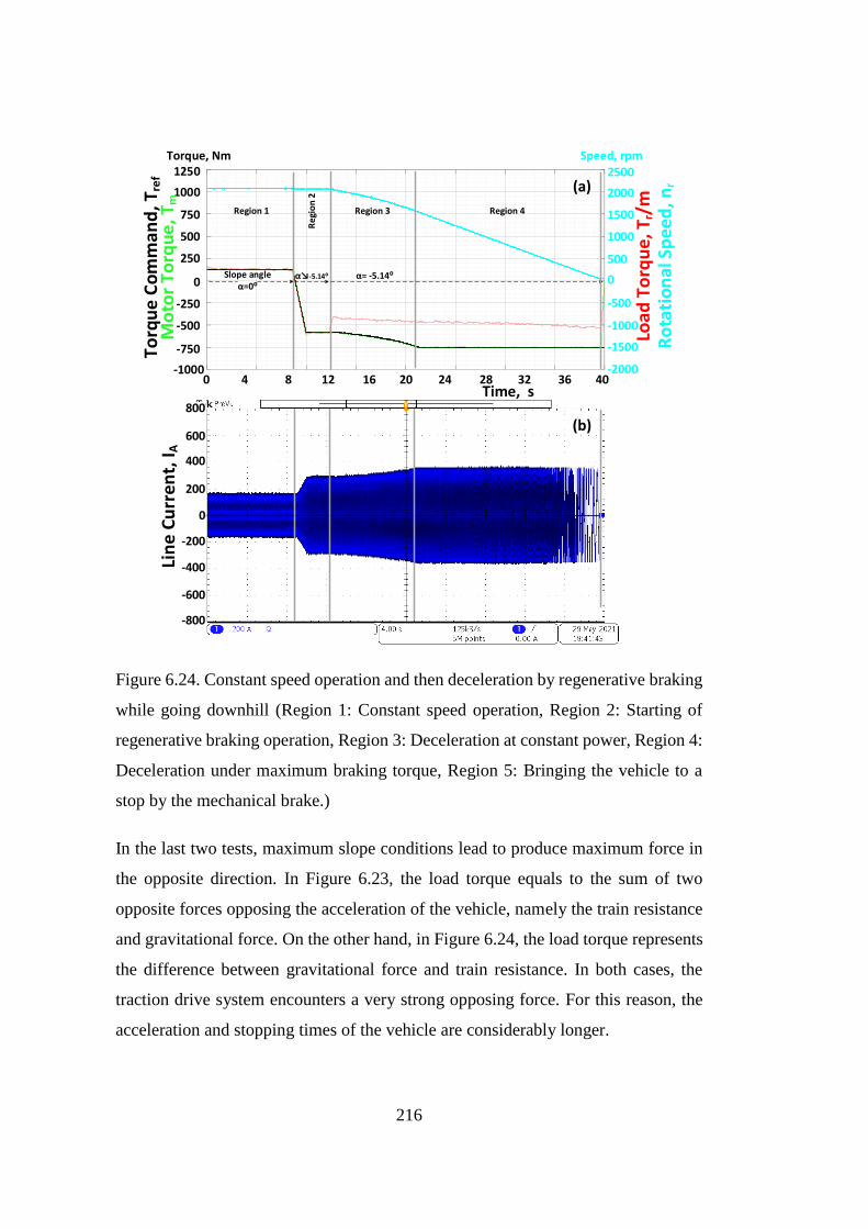
216

1500

-1000

1000

-500

500

2500

-1500

Loa

d T

orq

ue

, Tr/

m2000

0

-2000

-750

250

0

-250

-500

-1000

500

Time, s

750

8001250 Torque, Nm Speed, rpm

Slope angle α=0⁰

α= -5.14⁰ α -5.14⁰

Region 1

Re

gio

n 2

Region 3 Region 4

1000

Mo

tor

To

rqu

e, T

m

To

rqu

e C

om

ma

nd

, Tre

f

Ro

tati

on

al S

pe

ed

, nr

Lin

e C

urr

en

t, I

A

0

400

800

-400

-800

-600

-200

200

600

0 4 8 12 16 20 24 28 32 36 40

(a)

(b)

Figure 6.24. Constant speed operation and then deceleration by regenerative braking

while going downhill (Region 1: Constant speed operation, Region 2: Starting of

regenerative braking operation, Region 3: Deceleration at constant power, Region 4:

Deceleration under maximum braking torque, Region 5: Bringing the vehicle to a

stop by the mechanical brake.)

In the last two tests, maximum slope conditions lead to produce maximum force in

the opposite direction. In Figure 6.23, the load torque equals to the sum of two

opposite forces opposing the acceleration of the vehicle, namely the train resistance

and gravitational force. On the other hand, in Figure 6.24, the load torque represents

the difference between gravitational force and train resistance. In both cases, the

traction drive system encounters a very strong opposing force. For this reason, the

acceleration and stopping times of the vehicle are considerably longer.

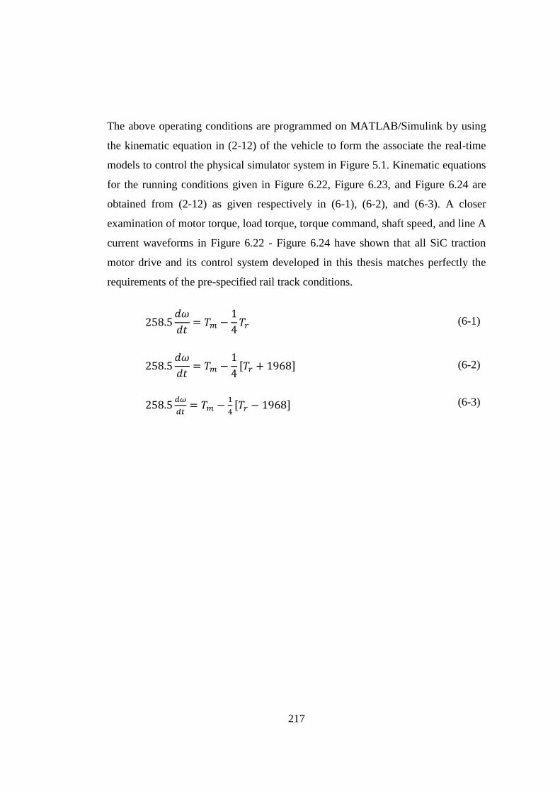
217

The above operating conditions are programmed on MATLAB/Simulink by using

the kinematic equation in (2-12) of the vehicle to form the associate the real-time

models to control the physical simulator system in Figure 5.1. Kinematic equations

for the running conditions given in Figure 6.22, Figure 6.23, and Figure 6.24 are

obtained from (2-12) as given respectively in (6-1), (6-2), and (6-3). A closer

examination of motor torque, load torque, torque command, shaft speed, and line A

current waveforms in Figure 6.22 - Figure 6.24 have shown that all SiC traction

motor drive and its control system developed in this thesis matches perfectly the

requirements of the pre-specified rail track conditions.

258.5

𝑑𝜔


1

4𝑇𝑟 (6-1)

258.5

𝑑𝜔


1

4[𝑇𝑟 + 1968] (6-2)

258.5𝑑𝜔


1

4[𝑇𝑟 − 1968] (6-3)

219

CHAPTER 7

7 FUTURE PROSPECTS OF SIC POWER MOSFETS IN POWER CONVERTERS

Increasing the efficiency of power converters has been one of the most important

issues that industry and academy have been working on for years. Today, the

increasing need for electrical energy use significantly creates more pressure for the

new pursuits to achieve increased power conversion efficiency. In academic studies

and thousands of exemplary applications in the industry, it is seen that Si-based

power semiconductors have reached their design limits in terms of breakdown

voltages, conduction, and switching losses. In order to overcome these problems, the

solutions based on parallel and serial use of semiconductors have been derived for

years. However, these solutions increase the system cost, bring application

difficulties and reduce product reliability due to the increase in the number of

components.

On the other hand, years of work have led to the widespread use of gallium nitride

(GaN) and silicon carbide (SiC) based wide bandgap power devices for high voltage

and power applications, which significantly improve the breakdown voltage,

conduction, and switching losses. The future perspective of GaN and SiC power

semiconductors are given in Figure 7.1.

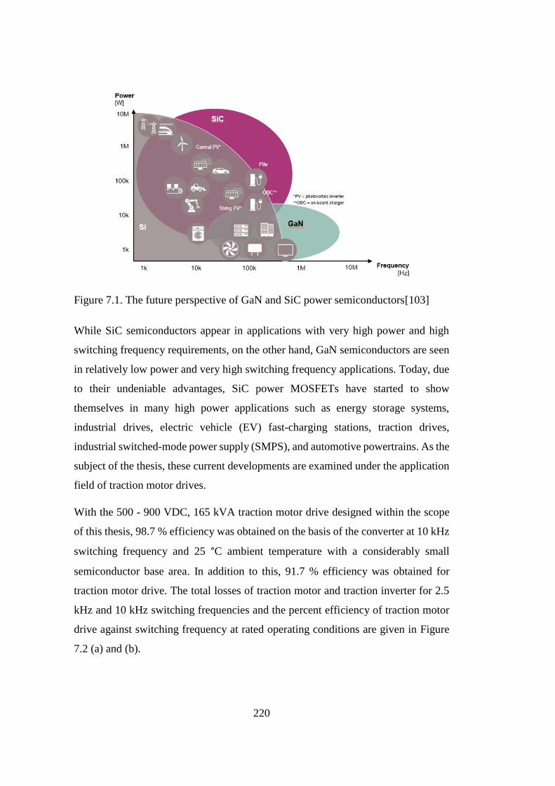
220

Figure 7.1. The future perspective of GaN and SiC power semiconductors[103]

While SiC semiconductors appear in applications with very high power and high

switching frequency requirements, on the other hand, GaN semiconductors are seen

in relatively low power and very high switching frequency applications. Today, due

to their undeniable advantages, SiC power MOSFETs have started to show

themselves in many high power applications such as energy storage systems,

industrial drives, electric vehicle (EV) fast-charging stations, traction drives,

industrial switched-mode power supply (SMPS), and automotive powertrains. As the

subject of the thesis, these current developments are examined under the application

field of traction motor drives.

With the 500 - 900 VDC, 165 kVA traction motor drive designed within the scope

of this thesis, 98.7 % efficiency was obtained on the basis of the converter at 10 kHz

switching frequency and 25 °C ambient temperature with a considerably small

semiconductor base area. In addition to this, 91.7 % efficiency was obtained for

traction motor drive. The total losses of traction motor and traction inverter for 2.5

kHz and 10 kHz switching frequencies and the percent efficiency of traction motor

drive against switching frequency at rated operating conditions are given in Figure

7.2 (a) and (b).

221

0

5000

10000

15000

1 2

10638

1331

9625

1679

Chart Title

Series1 Series2

91,2

91,3

91,4

91,5

91,6

91,7

91,8

0 1 2 3 4 5 6 7 8 9

Chart Title

Total Motor Losses

Total Semiconductor Losses

@ 2.5 kHz switchig frequency

@ 10 kHz switchig frequency

2.5 5 7.5 10 12.5 15 17.5 20

Pow

er L

oss

(W)

Effi

cie

ncy

(%)

Frequency, kHz

Traction Motor Drive Efficiency @ 165 kVA, 0.83 pf

Operating Switching Frequency

(a) (b)

Figure 7.2. (a) Total traction motor and traction inverter losses for 2.5 kHz and 10

kHz switching frequencies (b) Percent efficiency of traction motor drive against

switching frequency

The total loss of traction motor is decreased by almost 1 kW by changing switching

frequency from 2.5 kHz to 10 kHz, as shown in Figure 7.2 (a). It facilitates traction

motor cooling and helps to extend the lifetime of the winding insulation materials.

On the other hand, it causes an increase of nearly 350 W for the total power loss of

the traction inverter. Considering this power loss increase per switch, it corresponds

to an increase of about 58W and does not create unmanageable thermal stress on the

switches. As can be seen from Figure 7.2 (b), the total motor drive efficiency can be

improved further by almost 0.5 % with the switching frequency optimization. At the

10 kHz operating point, the calculated junction temperature of MOSFETs

approaches to 110 °C while the traction drive is operating at an ambient temperature

of 45 °C in nominal working conditions (i.e., 480 Vline-to-line, 165 kVA, and 60 Hz).

The junction temperatures at 12.5 kHz and 15 kHz switching frequencies are 113 °C

and 117 °C, respectively. In order not to shorten the lifetime of the switches, the

junction temperatures of the chips are kept minimum as much as possible. Each 10

°C increase in junction temperatures causes half the lifetime of the semiconductor.

Moreover, further increase of switching frequency beyond the 10 kHz does not

satisfy considerable advantages to improve system efficiency. Thus, 10 kHz

switching frequency was determined as optimum switching frequency, as explained

in Chapter 3.

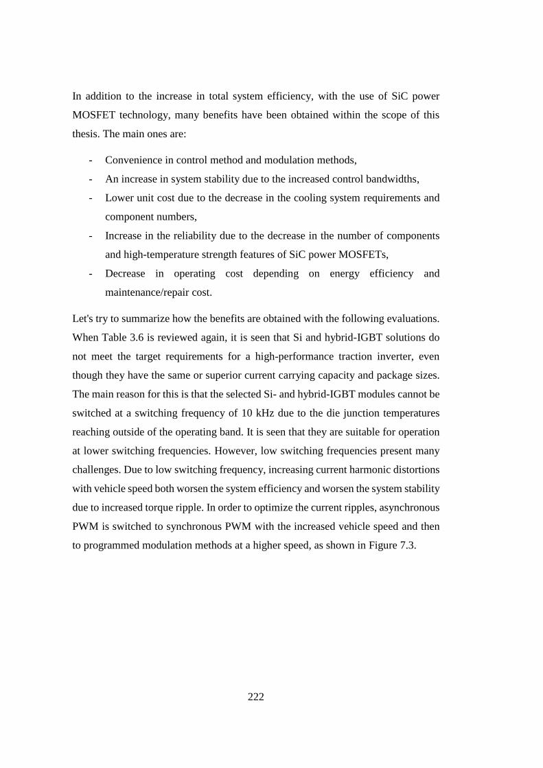
222

In addition to the increase in total system efficiency, with the use of SiC power

MOSFET technology, many benefits have been obtained within the scope of this

thesis. The main ones are:

- Convenience in control method and modulation methods,

- An increase in system stability due to the increased control bandwidths,

- Lower unit cost due to the decrease in the cooling system requirements and

component numbers,

- Increase in the reliability due to the decrease in the number of components

and high-temperature strength features of SiC power MOSFETs,

- Decrease in operating cost depending on energy efficiency and

maintenance/repair cost.

Let's try to summarize how the benefits are obtained with the following evaluations.

When Table 3.6 is reviewed again, it is seen that Si and hybrid-IGBT solutions do

not meet the target requirements for a high-performance traction inverter, even

though they have the same or superior current carrying capacity and package sizes.

The main reason for this is that the selected Si- and hybrid-IGBT modules cannot be

switched at a switching frequency of 10 kHz due to the die junction temperatures

reaching outside of the operating band. It is seen that they are suitable for operation

at lower switching frequencies. However, low switching frequencies present many

challenges. Due to low switching frequency, increasing current harmonic distortions

with vehicle speed both worsen the system efficiency and worsen the system stability

due to increased torque ripple. In order to optimize the current ripples, asynchronous

PWM is switched to synchronous PWM with the increased vehicle speed and then

to programmed modulation methods at a higher speed, as shown in Figure 7.3.

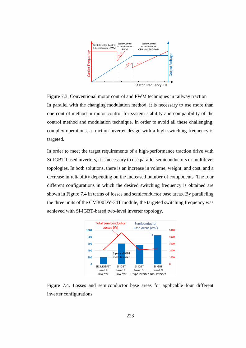
223

Car

rier

Fre

quen

cyStator Frequency, Hz

Field Oriented Control & Asynchronous PWM

Scalar Control & Synchronous

PWM

Scalar Control & Synchronous

OPWM or SHE-PWM

Ou

tpu

t V

olta

ge

Figure 7.3. Conventional motor control and PWM techniques in railway traction

In parallel with the changing modulation method, it is necessary to use more than

one control method in motor control for system stability and compatibility of the

control method and modulation technique. In order to avoid all these challenging,

complex operations, a traction inverter design with a high switching frequency is

targeted.

In order to meet the target requirements of a high-performance traction drive with

Si-IGBT-based inverters, it is necessary to use parallel semiconductors or multilevel

topologies. In both solutions, there is an increase in volume, weight, and cost, and a

decrease in reliability depending on the increased number of components. The four

different configurations in which the desired switching frequency is obtained are

shown in Figure 7.4 in terms of losses and semiconductor base areas. By paralleling

the three units of the CM300DY-34T module, the targeted switching frequency was

achieved with Si-IGBT-based two-level inverter topology.

0

1000

2000

3000

4000

5000

0

200

400

600

800

1000

1 2 3 4

Chart Title

Series1 Series2

SiC MOSFET based 2L Inverter

Si IGBT based 2L Inverter

Si IGBT based 3L

NPC Inverter

Si IGBT based 3L

T-type Inverter

Semiconductor Base Areas (cm2)

Total Semicondcutor Losses (W)

3 paralel IGBT modules used

Figure 7.4. Losses and semiconductor base areas for applicable four different

inverter configurations

224

In Figure 7.4, it can be seen that the SiC MOSFET-based two-level inverter is the

best topology in terms of efficiency and semiconductor base area. 10 kHz switching

frequency gives a chance to use common SVPWM as a modulation technique and

FOC method for motor control in all operating regions.

Many analyses and evaluations have been made within the scope of this thesis to

show that the benefits to be obtained with multilevel converters can also be achieved

with SiC MOSFET-based two-level inverters. Moreover, additional advantages such

as volume, weight, and reliability obtained with SiC MOSFET-based inverter are

also reported.

In addition to these, there are also studies that are still the subject of research and

whose distinction cannot be clearly demonstrated. One of these problems is

electromagnetic interference, and the other is related to the operating temperature. In

fact, there will be a positive reflection on electromagnetic interference due to the

almost zero reverse recovery charge (e.g., lower peak switching current). However,

parasitic capacitances also need to be optimized to avoid common-mode currents

that can occur with increasing switching speed. Moreover, due to increased

switching dynamics, parasitic inductances should be further reduced compared to

existing power modules in order to fulfill the electromagnetic compatibility

requirements and to guarantee operation in the safe operating area of

semiconductors. High switching speeds also have a great strain on motor windings

insulations and bearings. Therefore, it may be necessary to improve the motor

winding insulation materials. These are the points that need extra attention from an

electrical point of view. As for the evaluation of operating temperature, if the

targeted very high operating temperatures can be achieved with SiC MOSFETs, it is

considered that highly innovative solutions will be needed in cooling system

structures and laminated busbar designs. For example, if operating temperatures of

400-500 °C are reached, there may be serious increases in radiative heat transfer. It

is thought that this change will require design changes in many hardware, especially

laminated busbar and cooling system structures.

225

CHAPTER 8

8 CONCLUSIONS AND FUTURE WORKS

The design and implementation of 165 kVA all SiC MOSFET-based traction inverter

has been carried out in this research work. The prototype has been designed and

developed according to the sample light rail transportation vehicle properties, its

track, and operating profile. In order to validate the produced prototype, a 150kW

full-scale physical simulator which consists of a motor test bench, has been

successfully implemented in a low power laboratory, which consumes active power

from the AC grid much smaller than the installed capacity of the simulator to account

only for the losses. The developed prototype was validated by using this simulator.

The developed physical simulator can be used in the design, technology

development, and performance testing of various types of traction inverters. The

catenary model, rail-track model, and vehicle model have been satisfactorily

integrated into the developed system to allow the performance verification of a

vehicle formation on a real track in real-time. The use of SiC power MOSFETs

reduces the volume and improves efficiency and representation of transient changes

in catenary voltage in comparison with Si-IGBT devices in traction applications.

Since SiC MOSFETs can be switched at higher frequencies with much shorter turn-

on and turn–off times in comparison with Si-IGBT based traction converters, EMI

considerations such as shorter cabling, ceramic motor bearings, optimized laminated

bus, silver-plated flat braid grounding cables, and etc., are considered as an important

issue in the design of the simulator.

At the present time, converter size, weight reduction issues, and energy efficiency

improvements by employing new wide bandgap power semiconductors are the most

attractive topics. Additionally, the electromagnetic compatibility and reliability

issues of AC drives with wide bandgap power semiconductors such as GAN and SiC

are popular and intensive research areas. Many significant academic studies have

226

been conducted on these subjects over the ten years. However, performance issues

involving the effects on other system components in AC traction drives (e.g., motors,

cables, transformers, etc.) are important and yet not fully investigated and addressed.

Operating an inverter with high dv/dt rates is problematic for the insulation of motor

windings. The current harmonics are significantly reduced with the increased

frequency. On the other hand, the frequency of exposure to a high dv/dt rate is also

increasing. This situation will create a considerable effect on the lifetime of electric

motors. New generation traction motors with insulating materials having dv/dt

ratings higher than 10 kV/µs should be commercially available in the future in order

to take full advantage of SiC power converters. Moreover, the effects of wide

bandgap power semiconductors on optimum converter topology selection (e.g., two-

level, three-level, etc.), contributions of wide bandgap power semiconductors to the

FOC, direct torque control algorithms, and programmed PWM techniques that are

needed in medium voltage high power applications are significant and wait for

clarification.

Following conclusions can be summarized from the results of theoretical and

experimental works carried out within the scope of this thesis:

The conversion efficiency of traction converter is obtained higher than 98.7

% with 10 kHz switching frequency in both motoring and regenerative

braking mode of operations.

Very high quality current waveforms were obtained. Motor current

waveform THD was observed as 3.11 %.

The motor losses have been reduced by about 1 kW (e.g. 0.7 %

improvement).

The overall system efficiency (e.g. traction conv. & motor) is increased

almost 2 %.

Operating cost is decreased due to the increased system efficiency.

The system stability and dynamic performance of the system are increased.

227

Only one modulation and control technique were used in all operating

regions. Therefore, controller design has been simplified.

The audible noise level is reduced due to the high switching frequency.

Mechanical stresses on motor shaft, couplings, gearboxes are improved due

to the decreased torque ripple.

It has been observed that the power and voltage levels at which the transition

to multilevel converters will be increased in the case of using SiC MOSFET-

based semiconductors.

This work showed that SiC semiconductors allowed the use of simple

converter topologies in higher power and voltage levels.

The voltage waveforms at the motor terminals were examined and it was

observed that the dv/dt rates exceeded the design limits of current traction

motors. It has been revealed that with the further development of the SiC

semiconductors, even more challenging conditions will arise. It was

emphasized that the motor winding insulation material should be improved.

Fully isolated motor bearings should be used due to the increased frequency

of common mode voltages and currents.

In this thesis, all the above-mentioned issues are investigated to make contributions

to the high power and medium voltage traction drive applications. Although this

review gives an idea of the future benefits of SiC MOSFETs, the boundary on which

they will offer advantages over power and voltage levels is not clearly defined due

to the limited variety of SiC power semiconductor products. In addition to this, as

future studies, after the product variety of SiC MOSFETs is sufficiently increased,

the distortion effects caused by non-linear effects of power semiconductors on the

output current and voltage waveforms of SiC MOSFETs can be examined and

compared to IGBTs. Moreover, the reduced die area and thickness with the SiC

materials yields to decrease the thermal capacitances of semiconductors. Because of

this, the aging due to the thermal cycles is very important and waiting for an

228

investigation. Additionally, the short circuit current capacity of the SiC power

modules should be improved for railway traction applications, or advanced gate-

driver which satisfy very fast short circuit protection should be designed. The

increased switching speeds increase the voltage spikes and leakage currents, and

hence increasing electromagnetic interference. Finally, passive filters and active

gate-drivers can be considered to reduce dv/dt rates at motor terminals then these

solutions can be compared for system efficiency, cost, EMI and reliability.

229

REFERENCES

[1] “Stream Locomotives” https://en.wikipedia.org/wiki/Steam_locomotive.

[2] M. C. Duffy, 1880 – 1990 Electric Railways, 1990.

[3] A. Pankhurst, Electric Traction Systems 2014, Published by The Institution of

Engineering and Technology, London, United Kingdom, 2014. 2014.

[4] T. E. Salem and R. A. Wood, “1000-H Evaluation of a 1200-V, 880-A All-

SiC Dual Module,” IEEE Trans. Power Electron., vol. 29, no. 5, pp. 2192–

2198, May 2014.

[5] A. Merkert, T. Krone, and A. Mertens, “Characterization and Scalable

Modeling of Power Semiconductors for Optimized Design of Traction

Inverters with Si- and SiC-Devices,” IEEE Trans. Power Electron., vol. 29,

no. 5, pp. 2238–2245, May 2014.

[6] M. Imaizumi et al., “Remarkable Advances in SiC Power Device Technology

for Ultra High Power Systems,” in 2013 IEEE International Electron Devices

Meeting, pp. 6.5.1-6.5.4, Dec. 2013.

[7] S. Hazra, S. Madhusoodhanan, G. K. Moghaddam, K. Hatua, and S.

Bhattacharya, “Design Considerations and Performance Evaluation of 1200-

V 100-A SiC MOSFET-Based Two-Level Voltage Source Converter,” IEEE

Trans. Ind. Appl., vol. 52, no. 5, pp. 4257–4268, Sep. 2016.

[8] E. Wiesner, K. Masuda, and M. Joko, “New 1200V Full SiC Module with

800A Rated Current,” in 2015 17th European Conference on Power

Electronics and Applications (EPE’15 ECCE-Europe), pp. 1–9, Sep. 2015.

[9] Brenna, M., Foiadelli, F. and Zanineli, D., Electrical Railway Transportation

Systems, Published by John Wiley & Sons, Inc., Hoboken, New Jersey, 2018.

[10] M. Steiner, M. Klohr, and S. Pagiela, “Energy Storage System With Ultracaps

230

On Board of Railway Vehicles,” in 2007 European Conference on Power

Electronics and Applications, pp. 1–10, 2007.

[11] L. Mir, I. Etxeberria-Otadui, I. P. de Arenaza, I. Sarasola, and T. Nieva, “A

Supercapacitor Based Light Rail Vehicle: System Design and Operations

Modes,” in 2009 IEEE Energy Conversion Congress and Exposition, pp.

1632–1639, Sep. 2009.

[12] A. L. Allegre, A. Bouscayrol, J.-N. Verhille, P. Delarue, E. Chattot, and S. El-

Fassi, “Reduced-Scale-Power Hardware-in-the-Loop Simulation of an

Innovative Subway,” IEEE Trans. Ind. Electron., vol. 57, no. 4, pp. 1175–

1185, Apr. 2010.

[13] A. L. Allegre, A. Bouscayrol, P. Delarue, P. Barrade, E. Chattot, and S. El-

Fassi, “Energy Storage System With Supercapacitor for an Innovative

Subway,” IEEE Trans. Ind. Electron., vol. 57, no. 12, pp. 4001–4012, Dec.

2010.

[14] D. Iannuzzi and P. Tricoli, “Speed-Based State-of-Charge Tracking Control

for Metro Trains With Onboard Supercapacitors,” IEEE Trans. Power

Electron., vol. 27, no. 4, pp. 2129–2140, Apr. 2012.

[15] W. Wang et al., “A Novel Energy Management Strategy of Onboard

Supercapacitor for Subway Applications With Permanent-Magnet Traction

System,” IEEE Trans. Veh. Technol., vol. 63, no. 6, pp. 2578–2588, Jul. 2014.

[16] “EN 50388:2012 European Standard ‘Railway Applications - Power Supply

And Rolling Stock - Technical Criteria For The Coordination Between Power

Supply (Substation) And Rolling Stock To Achieve Interoperability’, 2012”.

[17] “EN 50163:2004 European Standard. ‘Railway Applications - Supply

Voltages Of Traction Systems’, November 2004”.

[18] R. J. Hill, “Electric railway traction. Part 1: Electric Traction and DC Traction

Motor Drives,” Power Eng. J., vol. 8, no. 1, pp. 47–56, Feb. 1994.

231

[19] R. J. Kemp, “Developments in Electric Traction,” Power Eng. J., vol. 3, no.

2, p. 71, 1989.

[20] D. Ronanki, S. A. Singh, and S. S. Williamson, “Comprehensive Topological

Overview of Rolling Stock Architectures and Recent Trends in Electric

Railway Traction Systems,” IEEE Trans. Transp. Electrif., vol. 3, no. 3, pp.

724–738, Sep. 2017.

[21] “https://www.mitsubishielectric-railway.eu/products-solutions/traction/vvvf-

inverter”.

[22] S. A. Azmi, K. H. Ahmed, S. J. Finney, and B. W. Williams, “Comparative

Analysis Between Voltage and Current Source Inverters in Grid-Connected

Application,” in IET Conference on Renewable Power Generation (RPG

2011), pp. 101–101, 2011.

[23] Y. Suh, J. K. Steinke, and P. K. Steimer, “Efficiency Comparison of Voltage-

Source and Current-Source Drive Systems for Medium-Voltage

Applications,” IEEE Trans. Ind. Electron., vol. 54, no. 5, pp. 2521–2531, Oct.

2007.

[24] Abad, G., ‘Power Electronics and Electric Drives for Traction Applications’,

Published by John Wiley & Sons, Inc., UK, 2017.

[25] D. Busse, J. Erdman, R. J. Kerkman, D. Schlegel, and G. Skibinski, “The

Effects of PWM Voltage Source Inverters on The Mechanical Performance of

Rolling Bearings,” in Proceedings of Applied Power Electronics Conference.

APEC ’96, vol. 2, pp. 561–5691,1996.

[26] S. Ogasawara and H. Akagi, “Modeling and Damping of High-Frequency

Leakage Currents in PWM Inverter-Fed AC Motor Drive Systems,” IEEE

Trans. Ind. Appl., vol. 32, no. 5, pp. 1105–1114, 1996.

[27] D. Busse, J. Erdman, R. J. Kerkman, D. Schlegel, and G. Skibinski, “System

Electrical Parameters and Their Effects on Bearing Currents,” IEEE Trans.

232

Ind. Appl., vol. 33, no. 2, pp. 577–584, 1997.

[28] L. Franquelo, J. Rodriguez, J. Leon, S. Kouro, R. Portillo, and M. Prats, “The

Age of Multilevel Converters Arrives,” IEEE Ind. Electron. Mag., vol. 2, no.

2, pp. 28–39, Jun. 2008.

[29] “States-of-the-art-review,” 2019, https://projects.shift2rail.org/s2r_matrixtd.

aspx.

[30] ECPE, “Position Paper Energy Efficiency – the Role of Power Electronics,”

2007.

[31] ECPE, “Next Generation Power Electronics based on Wide Bandgap Devices

- Challenges and Opportunities for Europe, ECPE Position Paper,” 2016.

[32] J. Rodriguez et al., “Multilevel Converters: An Enabling Technology for

High-Power Applications,” Proc. IEEE, vol. 97, no. 11, pp. 1786–1817, Nov.

2009.

[33] J. Zhang, J. Liu, S. Zhong, J. Yang, N. Zhao, and T. Q. Zheng, “A Power

Electronic Traction Transformer Configuration With Low-Voltage IGBTs for

Onboard Traction Application,” IEEE Trans. Power Electron., vol. 34, no. 9,

pp. 8453–8467, Sep. 2019.

[34] P. Simiyu, I. E. Davidson, “MVDC Railway Traction Power Systems; State-

of-the Art, Opportunities, and Challenges,” Energies 2021, vol. 14, p. 4156,

2021.

[35] S. Singh, “IGCT Transient Analysis and Clamp Circuit Design for VSC

valves,” Master Thesis, Royal Inst. Technol. (KTH), Stock., 2012.

[36] Y. Shakweh, “New Breed of Medium Voltage Converters,” Power Eng. J.,

vol. 14, no. 1, pp. 12–20, Feb. 2000.

[37] S. Bernet, “Recent Developments of High Power Converters for Industry and

Traction Applications,” IEEE Trans. Power Electron., vol. 15, no. 6, pp.

233

1102–1117, Nov. 2000.

[38] “https://www.fujielectric-europe.com/en/power_semiconductor.”

[39] “https://www.hitachiabb-powergrids.com/offering/product-and-

system/semiconductors.”

[40] “https://www.infineon.com/cms/en/product/power/igbt/igbt-

modules/#!products,” 2021.

[41] “https://www.mitsubishielectric.com/semiconductors/products/powermod/

index.html.”

[42] “https://www.wolfspeed.com/products/power/sic-power-modules.”

[43] B. Wu, High-Power Converters and AC Drives, Piscataway, NJ, IEEE Press,

2006.

[44] Integrated gate-commutated thyristors, ABB Switzerland Ltd, IGCT flyer,

Doc. No. 5SYA2023, April 2008. http://www.abb.com/semiconductors.

[45] R. D. Klug, N. Klaassen, “High Power Medium Voltage Drives - Innovations,

Portfolio, Trends,” 2005 European Conference on Power Electronics and

Applications, pp. 10 pp, 2005.

[46] R. Alvarez, F. Filsecker, and S. Bernet, “Characterization of a new 4.5 kV

press pack SPT+ IGBT for medium voltage converters,” in 2009 IEEE Energy

Conversion Congress and Exposition, pp. 3954–3962, Sep. 2009.

[47] J. Fabre, P. Ladoux, and M. Piton, “Characterization and Implementation of

Dual-SiC MOSFET Modules for Future Use in Traction Converters,” IEEE

Trans. Power Electron., vol. 30, no. 8, pp. 4079–4090, Aug. 2015.

[48] J. Fabre and P. Ladoux, “Parallel Connection of 1200-V/100-A SiC-MOSFET

Half-Bridge Modules,” IEEE Trans. Ind. Appl., vol. 52, no. 2, pp. 1669–1676,

2016.

[49] P. Hofstetter and M. M. Bakran, “The Two-Dimensional Short-Circuit

234

Detection Protection for SiC MOSFETs in Urban Rail Transit Application,”

IEEE Trans. Power Electron., vol. 35, no. 6, pp. 5692–5701, Jun. 2020.

[50] T. W. McNairy, “High-Speed Circuit Breakers,” 1928.

[51] D. L. S. Marson, “High Speed Rail Electric-Power Supply Network,” Thesis,

Czech Tech. Univ. Prague, 2016.

[52] “http://www.ejrcf.or.jp/jrtr/jrtr20/pdf/F52_Tech.pdf.”

[53] https://www.i-sis.org.uk/Supercapacitors_for_Flexible_Energy_Storage.php

[54] A. Jongeling, “Optimising the Input Filter of Traction Installations in DC

Railway Power Systems,” Master Thesis, Delft Univ. Technol., pp. 1–146,

2017.

[55] Y. Zhu, “Adhesion in the Wheel – Rail Contact”, Thesis, Royal Institute of

Technology, 2013.

[56] M. Kondo, M. Miyabe, R. Ebizuka, and K. Hanaoka, “Design and Efficiency

Evaluation of a High-Efficiency Induction Motor for Railway Traction,”

Electr. Eng. Japan (English Transl. Denki Gakkai Ronbunshi), vol. 194, no.

2, pp. 15–23, 2016.

[57] Z. Tian, “System Energy Optimisation Strategies for DC Railway Traction

Power Networks,” University of Birmingham.

[58] A. F. Abouzeid et al., “Control Strategies for Induction Motors in Railway

Traction Applications,” Energies, vol. 13, no. 3. p. 700, Feb. 06, 2020.

[59] S. Mohammad, M. Gazafrudi, A. T. Langerudy, E. F. Fuchs, and K. Al-

haddad, “Power Quality Issues in Railway Electrification : A Comprehensive

Perspective,” IEEE Trans. Ind. Electron., vol. 62, no. 5, pp. 3081–3090, 2015.

[60] A. Choudhury, “Three-Level Neutral Point Clamped ( NPC ) Traction

Inverter Drive for Electric Vehicles, Electrical and Computer Engineering

Presented in Partial Fulfillment of the Requirements for the Degree of Doctor

235

of Philosophy Electrical and Comp,” no. April, 2015.

[61] J. M. Knezevic, “Low-Cost Low-Resolution Sensorless Positioning of DC

Motor Drives for Vehicle Auxiliary Applications,” IEEE Trans. Veh.

Technol., vol. 62, no. 9, pp. 4328–4335, Nov. 2013.

[62] J. Brenneisen, E. Futterlieb, E. Muller, and M. Schulz, “A New Converter

Drive System for a Diesel Electric Locomotive with Asynchronous Traction

Motors,” IEEE Trans. Ind. Appl., vol. IA-9, no. 4, pp. 482–491, Jul. 1973.

[63] I. Press and R. Perez, Electrical Railway Transportation Systems, Hoboken,

NJ, USA: John Wiley & Sons, Inc., 2018.

[64] R. Krishnan, “Permanent Magnet Synchronous and Brushless DC Motor

Drives”, London New York, CRC Press, 2010.

[65] G. Pellegrino, A. Vagati, B. Boazzo, and P. Guglielmi, “Comparison of

induction and PM synchronous motor drives for EV application including

design examples,” IEEE Trans. Ind. Appl., vol. 48, no. 6, pp. 2322–2332,

2012.

[66] D. A. Rendusara, “Analysis of Some Application Aspect in Modern (PWM)

Adjustable Speed Drive Systems and New Solutions,” Texas A&M

University, 2000.

[67] P. M. Page, HIGH-POWER CONVERTERS and AC Drives. 2007.

[68] A. L. Julian, G. Oriti, and T. A. Lipo, “Elimination of common-mode voltage

in three-phase sinusoidal power converters,” IEEE Trans. Power Electron.,

vol. 14, no. 5, pp. 982–989, Sep. 1999.

[69] M. M. Swamy and S. L. Rossiter, “Harmonic Interaction Between 1500 kVA

Supply Transformer and VFD Load at an Industrial Plant,” IEEE Trans. Ind.

Appl., vol. 34, no. 5, pp. 897–903, 1998.

[70] A. Salem and M. A. Abido, “T-Type Multilevel Converter Topologies: A

236

Comprehensive Review,” Arab. J. Sci. Eng., vol. 44, no. 3, pp. 1713–1735,

2019.

[71] K. Yamanaka, A. M. Hava, H. Kirino, Y. Tanaka, N. Koga, and T. Kume, “A

Novel Neutral Point Potential Stabilization Technique Using the Information

of Output Current Polarities and Voltage Vector,” IEEE Trans. Ind. Appl.,

vol. 38, no. 6, pp. 1572–1580, Nov. 2002.

[72] M. Koyama, T. Fujii, R. Uchida, and T. Kawabata, “Space Voltage Vector-

Based New PWM Method for Large Capacity Three-Level GTO Inverter,” in

Proceedings of the 1992 International Conference on Industrial Electronics,

Control, Instrumentation, and Automation, pp. 271–276, 1992.

[73] E. Ün, “Common Mode Voltage and Current Reduction in Voltage Source

Inverter Driven Three Phase AC Motors,” Middle East Technical University,

2007.

[74] A. M. Hava, R. J. Kerkman, and T. A. Lipo, “Carrier-based PWM-VSI

overmodulation strategies: analysis, comparison, and design,” IEEE Trans.

Power Electron., vol. 13, no. 4, pp. 674–689, Jul. 1998.

[75] Lipo Thomas A.; D. Grahame Holmes, Pulse Width Modulation For Power

Converters. 2003.

[76] “A.M. Hava, ‘Carrier Based PWM-VSI Drives in the Overmodulation

Region,’ Ph.D. Thesis, University of Wisconsin-Madison, 1998.”

[77] Y. He, “A Comparison of Modulation Techniques and Motor Performance

Evaluation,” Master Thesis, Chalmers Univ. Technol., 2018.

[78] G. S. Buja and G. B. Indri, “Optimal Pulsewidth Modulation for Feeding AC

Motors,” IEEE Trans. Ind. Appl., vol. IA-13, no. 1, pp. 38–44, Jan. 1977.

[79] G. Narayanan and V. T. Ranganathan, “Two Novel Synchronized Bus-

Clamping PWM Strategies Based on Space Vector Approach for High Power

Drives,” IEEE Trans. Power Electron., vol. 17, no. 1, pp. 84–93, Jan. 2002.

237

[80] J. Napoles, J. I. Leon, R. Portillo, L. G. Franquelo, and M. A. Aguirre,

“Selective Harmonic Mitigation Technique for High-Power Converters,”

IEEE Trans. Ind. Electron., vol. 57, no. 7, pp. 2315–2323, Jul. 2010.

[81] J. Lago and M. L. Heldwein, “Generalized Synchronous Optimal Pulse Width

Modulation for Multilevel Inverters,” IEEE Trans. Power Electron., vol. 32,

no. 8, pp. 6297–6307, Aug. 2017.

[82] F. Niu, B. Wang, A. S. Babel, K. Li, and E. G. Strangas, “Comparative

Evaluation of Direct Torque Control Strategies for Permanent Magnet

Synchronous Machines,” IEEE Trans. Power Electron., vol. 31, no. 2, pp.

1408–1424, Feb. 2016.

[83] M. Rashed, P. F. A. MacConnell, A. F. Stronach, and P. Acarnley, “Sensorless

Indirect-Rotor-Field-Orientation Speed Control of a Permanent-Magnet

Synchronous Motor With Stator-Resistance Estimation,” IEEE Trans. Ind.

Electron., vol. 54, no. 3, pp. 1664–1675, Jun. 2007.

[84] I. Takahashi and T. Noguchi, “A New Quick-Response and High-Efficiency

Control Strategy of an Induction Motor,” IEEE Trans. Ind. Appl., vol. IA-22,

no. 5, pp. 820–827, Sep. 1986.

[85] N. R. N. Idris and A. H. M. Yatim, “Direct Torque Control of Induction

Machines With Constant Switching Frequency and Reduced Torque Ripple,”

IEEE Trans. Ind. Electron., vol. 51, no. 4, pp. 758–767, Aug. 2004.

[86] G. K. Singh, K. Nam, and S. K. Lim, “A Simple Indirect Field-Oriented

Control Scheme for Multiphase Induction Machine,” IEEE Trans. Ind.

Electron., vol. 52, no. 4, pp. 1177–1184, Aug. 2005.

[87] R. Bojoi, M. Lazzari, F. Profumo, and A. Tenconi, “Digital Field-Oriented

Control for Dual Three-Phase Induction Motor Drives,” IEEE Trans. Ind.

Appl., vol. 39, no. 3, pp. 752–760, May 2003.

[88] J. Rodriguez, R. M. Kennel, J. R. Espinoza, M. Trincado, C. A. Silva, and C.

238

A. Rojas, “High-Performance Control Strategies for Electrical Drives: An

Experimental Assessment,” IEEE Trans. Ind. Electron., vol. 59, no. 2, pp.

812–820, Feb. 2012.

[89] H. Kubota and K. Matsuse, “Speed Sensorless Field-Oriented Control of

Induction Motor with Rotor Resistance Adaptation,” IEEE Trans. Ind. Appl.,

vol. 30, no. 5, pp. 1219–1224, 1994.

[90] I. Takahashi and Y. Ohmori, “High-Performance Direct Torque Control of an

Induction Motor,” IEEE Trans. Ind. Appl., vol. 25, no. 2, pp. 257–264, 1989.

[91] H. Kubota, K. Matsuse, and T. Nakano, “DSP-Based Speed Adaptive Flux

Observer of Induction Motor,” IEEE Trans. Ind. Appl., vol. 29, no. 2, pp. 344–

348, 1993.

[92] D. Casadei, F. Profumo, G. Serra, and A. Tani, “FOC and DTC: Two Viable

Schemes for Induction Motors Torque Control,” IEEE Trans. Power

Electron., vol. 17, no. 5, pp. 779–787, Sep. 2002.

[93] D. Yildirim et al., “Full-Scale Physical Simulator of All SiC Traction Motor

Drive With Onboard Supercapacitor ESS for Light-Rail Public

Transportation,” IEEE Trans. Ind. Electron., vol. 67, no. 8, pp. 6290–6301,

Aug. 2020.

[94] “AN6156 Calculating Power Losses in an IGBT Module Application Note.”

https://www.dynexsemi.com/Portals/0/assets/downloads/DNX_AN6156.pdf.

[95] L. Buhrkall, “Traction System Case Study,” in IET Professional Development

Course on Electric Traction Systems, pp. 45–63, 2008.

[96] M. Youssef, J. Abu-Qahouq, and M. Orabi, “The Electromagnetic

Compatibility Design Considerations of the Input Filter of a 3-Phase Inverter

in a Railway Traction System,” in 2010 IEEE Energy Conversion Congress

and Exposition, pp. 4210–4216, Sep. 2010.

[97] “https://www.secheron.com/products-solutions/ess/dc-circuit-breakers-2/for-

239

rail-vehicles/.”

[98] Jin Wang, “Practical Design Considerations of Power Electronics in Hybrid

and Fuel Cell Vehicles,” in 2008 IEEE Vehicle Power and Propulsion

Conference, pp. 1–6, Sep. 2008.

[99] “https://ep-us.mersen.com/sites/mersen_us/files/2020-03/Mersen-Solutions-

for-SiC-Inverter.pdf,” 2021.

[100] “https://www.fischerelektronik.de/web_fischer/en_GB/heatsinks/D01/High-

performance%20heatsinks/$catalogue/fischerData/PR/SK461_/search.xhtml,

” 2021.

[101] IEC, “Rotating Electrical Machines - Part 25: AC Electrical Machines Used

in Power Drive Systems - Application Guide,” no. 60034–25, p. 64, 2014.

[102] B. S. I. S. Publication, “Rotating Electrical Machines Part 18–41: Partial

Discharge Free Electrical Insulation Systems (Type I) Used in Rotating

Electrical Machines Fed from Voltage Converters — Qualification and

Quality Control Tests,” no. Type I, 2011.

[103] “https://www.infineon.com/cms/en/product/wide-band-gap-semiconductors-

sic-gan/,” 2021.

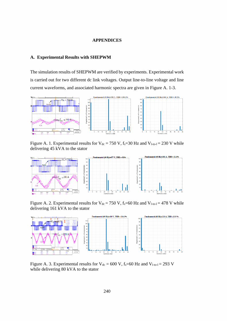
240

APPENDICES

A. Experimental Results with SHEPWM

The simulation results of SHEPWM are verified by experiments. Experimental work

is carried out for two different dc link voltages. Output line-to-line voltage and line

current waveforms, and associated harmonic spectra are given in Figure A. 1-3.

Figure A. 1. Experimental results for Vdc = 750 V, fs=30 Hz and Vl-to-l = 230 V while

delivering 45 kVA to the stator

Figure A. 2. Experimental results for Vdc = 750 V, fs=60 Hz and Vl-to-l = 478 V while

delivering 161 kVA to the stator

Figure A. 3. Experimental results for Vdc = 600 V, fs=60 Hz and Vl-to-l = 293 V

while delivering 80 kVA to the stator

241

CURRICULUM VITAE

PERSONAL INFORMATION

Surname, Name: Yıldırım, Doğan

Nationality: Turkish (TC)

Date and Place of Birth: 10 Eylül 1985, Çorum

Marital Status: Married

Phone: +90 312 210 22 92

Fax: +90 312 210 22 91

email: [email protected]

EDUCATION

Degree Institution Year of

Graduation

MS METU Electrical and Electronics Eng. 2012

BS METU Electrical and Electronics Eng. 2008

High School Kırıkkale Anadolu High School 2003

WORK EXPERIENCE

Year Place Enrollment

2018-Present

2015-2018

2012-2015

2008-2012

ASELSAN

ASELSAN

ASELSAN

ASELSAN

Lead Design Engineer

Senior Design Engineer

Expert Design Engineer

Design Engineer

2007 July GATE Elektronik Intern Eng. Student

2006 August ASELSAN Intern Eng. Student

FOREIGN LANGUAGES

English

PUBLICATIONS

1. Yıldırım, D., Öztürk, S., Çadırcı, I., Ermiş, M., “All SiC PWM Rectifier-Based

Off-board Ultrafast Charger for Heavy Electric Vehicles”, IET Power

Electronics , vol. 13, issue. 3, 2020, pp. 483-494.

242

2. Yıldırım, D., Akşit, M. H., Yolaçan, C., “Full-Scale Physical Simulator of All

SiC Traction Motor Drive with Onboard Supercapacitor ESS for Light-Rail

Public Transportation”, IEEE Transactions on Industrial Electronics, vol. 67,

issue. 8, 2020, pp. 6290-6301.

3. Nalçaçı, G., Yıldırım, D. and Ermiş, M., “Selective Harmonic Elimination for

Light-Rail Transportation Motor Drives using Harris Hawks Algorithm”,

Proceedings of 2020 IEEE International Conference on Environment and

Electrical Engineering and 2020 IEEE Industrial and Commercial Power

Systems Europe (EEEIC / I&CPS Europe), June. 9-12, 2020.

Documents

ALL SIC TRACTION CONVERTER FOR LIGHT RAIL