C A R F W o r k i n g P a p e r

CARF-F-166

Alternative Asymmetric Stochastic Volatility Models

Manabu Asai

Soka University Michael McAleer

Erasmus University Rotterdam Tinbergen Institute

The University of Tokyo

August 2009

CARF is presently supported by Bank of Tokyo-Mitsubishi UFJ, Ltd., Citigroup, Dai-ichi Mutual Life Insurance Company, Meiji Yasuda Life Insurance Company, Nippon Life Insurance Company, Nomura Holdings, Inc. and Sumitomo Mitsui Banking Corporation (in alphabetical order). This financial support enables us to issue CARF Working Papers.

CARF Working Papers can be downloaded without charge from: http://www.carf.e.u-tokyo.ac.jp/workingpaper/index.cgi

Working Papers are a series of manuscripts in their draft form. They are not intended for circulation or distribution except as indicated by the author. For that reason Working Papers may not be reproduced or distributed without the written consent of the author.

1

Alternative Asymmetric Stochastic Volatility Models*

Manabu Asai

Faculty of Economics Soka University, Japan

Michael McAleer Econometric Institute

Erasmus School of Economics Erasmus University Rotterdam

and Tinbergen Institute The Netherlands

and Center for International Research on the Japanese Economy (CIRJE)

Faculty of Economics University of Tokyo

Revised: August 2009

* The authors wish to acknowledge the insightful comments and suggestions of the Editor and a referee, and helpful discussions with Felix Chan, Neil Shephard and Jun Yu, and seminar participants at Fondazione Eni Enrico Mattei - Milan, National University of Singapore, University of Auckland, University of Melbourne, University of Milan-Bicocca, University of Venice “Ca’ Foscari”, Ente Einaudi - Rome, and University Pompeu Fabra. An earlier version of the paper was presented at the Symposium on Econometric Forecasting and High-Frequency Data Analysis in Singapore, May 2004. The first author appreciates the financial support of the Japan Society for the Promotion of Science, and the Australian Academy of Science. The second author is grateful for the financial support of the Australian Research Council.

2

Abstract

The stochastic volatility model usually incorporates asymmetric effects by introducing the negative correlation between the innovations in returns and volatility. In this paper, we propose a new asymmetric stochastic volatility model, based on the leverage and size effects. The model is a generalization of the exponential GARCH (EGARCH) model of Nelson (1991). We consider categories for asymmetric effects, which describes the difference among the asymmetric effect of the EGARCH model, the threshold effects indicator function of Glosten, Jagannathan and Runkle (1992), and the negative correlation between the innovations in returns and volatility. The new model is estimated by the efficient importance sampling method of Liesenfeld and Richard (2003), and the finite sample properties of the estimator are investigated using numerical simulations. Four financial time series are used to estimate the alternative asymmetric SV models, with empirical asymmetric effects found to be statistically significant in each case. The empirical results for S&P 500 and Yen/USD returns indicate that the leverage and size effects are significant, supporting the general model. For TOPIX and USD/AUD returns, the size effect is insignificant, favoring the negative correlation between the innovations in returns and volatility. We also consider standardized t distribution for capturing the tail behavior. The results for Yen/USD returns show that the model is correctly specified, while the results for three other data sets suggest there is scope for improvement. Key words: Stochastic volatility, asymmetric effects, leverage, threshold, indicator function, importance sampling, numerical simulations.

3

1 Introduction

It has long been recognized that the returns of financial assets are negatively correlated with changes in the volatilities of returns (see Black (1976) and Christie (1982)) and, moreover, that such volatilities tend to change over time. In the class of autoregressive conditional heteroskedasticity (ARCH) models pioneered by Engle (1982), several authors have proposed extensions of the ARCH model and found evidence of such negative correlation. For instance, Nelson (1991) proposed the exponential generalized ARCH (EGARCH) model, while Glosten, Jagannathan and Runkle (1992) developed GJR, a threshold indicator function GARCH model. The threshold effect is typically called asymmetry when the threshold is set to zero. A common idea used in such asymmetric models is the ‘leverage’ effect, in which negative shocks to returns increase the predictable volatility to a greater extent than do positive shocks of a similar magnitude.

On the other hand, stochastic volatility (SV) models are based on the direct

correlation between the innovations in both returns and volatility. For a theoretical development in continuous time, Hull and White (1987) generalized the Black-Scholes option pricing formula to analyse stochastic volatility and the negative correlation between the innovations. In empirical research, extensions of a simple discrete time model due to Taylor (1986) have been analysed by Wiggins (1987), Chesney and Scott (1989), and Harvey and Shephard (1996) in order to accommodate the direct correlation. Although this extension has been called the asymmetric SV model, we will refer to the asymmetric behaviour based on the direct correlation between the innovations as the “leverage” SV (SV-L) model to distinguish it from an alternative model of asymmetry. A comparison of a variety of univariate and multivariate, conditional and stochastic, models is given in McAleer (2005).

In addition to the leverage model, this paper considers a general asymmetric SV

model based on the EGARCH specification of Nelson (1991). As the EGARCH model incorporates both leverage and size effects, we will refer to the asymmetric behaviour as the “leverage and size effects” SV (SV-LS) model. The SV-LS model nests the SV-L model. As another special case of the SV-LS model, we will also consider the “size effect” SV (SV-S) model, which is a symmetric model. The SV-LS model will be estimated and tested for an optimal and practical representation of asymmetry. The general model also permits the non-nested SV-L and SV-S models to be tested against

4

each other. Recently, So et al. (2002) considered a threshold effects model in which the breaks in the constant and autoregressive parameter in the SV equation depend on the signs of the previous returns. Their model will not be discussed in detail here as the empirical results in Asai and McAleer (2005) show that their model is generally inferior to the SV-L model given below in terms of the AIC and BIC criteria.

The empirical analysis is concerned with both stock returns and exchange rate

returns. Although Gallant, Hsieh and Tauchen (1991) found that the response of conditional volatility to negative and positive shocks was essentially symmetric for the British pound/US dollar exchange rate by using the seminonparametric technique of Gallant and Tauchen (1989), we observed asymmetries in the exchange rate data based on the SV-L and SV-S models, even though such asymmetries may not be captured adequately using the ARCH approach. In addition to providing more accurate estimates of volatility, these empirical results should assist in calculating optimal Value-at-Risk (VaR) forecasts and capital charges for purposes of portfolio and risk management.

For estimation of the SV model, recent developments have been on the likelihood-oriented procedures (see Fridman and Harris (1998), Sandmann and Koopman (1998), Liesenfeld and Richard (2003)), and on the Bayesian Markov Chain Monte Carlo (MCMC) technique proposed by Jacquier, Polson and Rossi (1994) (see, among others, Chib, Nardari and Shephard (2002) and Shephard and Pitt (1998)). The Monte Carlo results conducted by Fridman and Harris (1998) and Sandmann and Koopman (1998) show that the properties of these methods are very similar to those of Jacquier, Polson and Rossi (1994). While the procedures proposed by Fridman and Harris (1998) are more computationally demanding than the MCMC technique of Jacquier, Polson and Rossi (1994), the simulated maximum likelihood approaches proposed by Sandmann and Koopman (1998) and Liesenfeld and Richard (2003) are much easier to implement computationally. Although the Monte Carlo likelihood method of Sandmann and Koopman (1998) is computationally faster, the efficient importance sampling (EIS) method of Liesenfeld and Richard (2003) is flexible to various kinds of SV models. With regard to the Bayesian approach, Asai (2005) compared several methods with regard to a numerical efficiency measure that was proposed by Geweke (1992).

The remainder of the paper is organized as follows. Section 2 examines the SV-L,

SV-S and SV-LS models, and investigates their relationships. A non-nested testing

5

procedure to discriminate between the SV-L and SV-S models is also discussed. Section 3 compares a variety of leverage and asymmetric effects in the framework of both stochastic and conditional volatility models. Section 4 discusses some standard estimation techniques for SV models, and Section 5 presents the results of Monte Carlo experiments regarding the finite sample performance of the estimators of the alternative SV models. In Section 6, the two asymmetric SV models and the SV-LS model are estimated using S&P 500 Composite returns, the Tokyo stock price index (TOPIX) returns, and the exchange rates between the USA and Australia and between Japan and the USA. Section 7 gives some concluding remarks. 2 Leverage and Asymmetry in SV Models

In this paper we consider a new asymmetric SV model. Before going to the SV class, we review the typical models for the ARCH class. There are two standard methods of capturing asymmetric behaviour in ARCH-type models, one of which is the exponential generalized ARCH (EGARCH) model of Nelson (1991). Although the EGARCH model has been used quite frequently in empirical applications when asymmetric behaviour is observed, the presence of the absolute value of a standardized shock in the model poses a problem regarding the statistical properties of the model.

The other frequently used model of asymmetric behaviour in ARCH-type models

is the threshold indicator function ARCH model of Glosten, Jagannathan and Runkle (1992) (GJR). This effect is typically called asymmetry when the threshold is set to zero, in which case a distinction is made between the effects of positive and negative shocks on volatility. But, as shown in the next section, the GJR model is very limited to express various kinds of asymmetries. The problem of EGARCH comes from the evaluation of the derivatives based on the absolute value of the standardized residuals. As shown in Hentschel (1995), we can avoid the problem by the two ways; one is to estimate the mean and variance equations separately, and the other is to approximate the absolute value function by using the rectangular hyperbola rotated counterclockwise by 45 degrees. As we can handle the problem of absolute values, the new asymmetric SV model will be based on the EGARCH model.

In this paper we consider the new asymmetric SV model, as follows:

6

exp( / 2), ~ (0,1), 1,..., ,t t t ty h N t Tε ε= = (1)

( ) { } 21 1 21 , ~ (0, ),t t t t t t th h E N ηφ μ φ γ ε γ ε ε η η σ+ = − + + + − + (2)

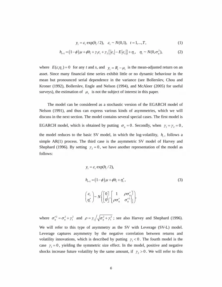
where ( ) 0t sE ε η = for any t and s, and t t ty R μ= − is the mean-adjusted return on an asset. Since many financial time series exhibit little or no dynamic behaviour in the mean but pronounced serial dependence in the variance (see Bollerslev, Chou and Kroner (1992), Bollerslev, Engle and Nelson (1994), and McAleer (2005) for useful surveys), the estimation of tμ is not the subject of interest in this paper. The model can be considered as a stochastic version of the EGARCH model of Nelson (1991), and thus can express various kinds of asymmetries, which we will discuss in the next section. The model contains several special cases. The first model is

EGARCH model, which is obtained by putting 0ησ = . Secondly, when 1 2 0γ γ= = ,

the model reduces to the basic SV model, in which the log-volatility, th , follows a simple AR(1) process. The third case is the asymmetric SV model of Harvey and Shephard (1996). By setting 2 0γ = , we have another representation of the model as follows:

( )1

2

exp( / 2),

1 ,

10~ , ,

0

t t t

t t t

t

t

y h

h h

N η

η η

ε

φ μ φ η

ε ρση ρσ σ

∗+

∗

∗ ∗ ∗

=

= − + +

⎛ ⎞⎡ ⎤⎛ ⎞ ⎡ ⎤⎜ ⎟⎢ ⎥⎜ ⎟ ⎢ ⎥⎜ ⎟⎢ ⎥⎣ ⎦⎝ ⎠ ⎣ ⎦⎝ ⎠

(3)

where 2 2 21η ησ σ γ∗ = + and 2 2

1 1ηρ γ σ γ= + ; see also Harvey and Shephard (1996).

We will refer to this type of asymmetry as the SV with Leverage (SV-L) model. Leverage captures asymmetry by the negative correlation between returns and volatility innovations, which is described by putting 1 0γ < . The fourth model is the case 1 0γ = , yielding the symmetric size effect. In the model, positive and negative shocks increase future volatility by the same amount, if 2 0γ > . We will refer to this

7

model as the SV with size effects (SV-S) model. The general model (1) and (2), which we will refer to the SV with leverage and size effects (SV-LS) model, can be considered as an extension of Asai and McAleer (2005). While Asai and McAleer (2005) is based on the unstandardized error, ty , the SV-LS model is based on the standardized error, tε . Hence, the SV-LS model capture standardized size effects.

The first and second moments of the generalized error term,

{ }1 2t t t t tEξ γ ε γ ε ε η≡ + − + ,

is given by ( ) 0tE ξ = and ( ) ( )2 2 2 2 21 2 1 2tEξ ησ ξ γ γ π σ≡ = + − + . The correlation

coefficient between tε and tξ is 1 ξγ σ .

In the class of SV, when 1 0γ ≠ and 2 0γ ≠ in, this yields our asymmetric SV model, which may be interpreted as either: (i) an asymmetric model which exhibits both leverage and thresholds; or (ii) an artifact which is used solely for purposes of testing the non-nested SV-L and SV-S models against each other. In the latter case, the four possible outcomes of the non-nested tests of the SV-L and SV-S models against each other are as follows: (i) 1 0γ = and 2 0γ = , which leads to rejection of both SV-L and SV-S; (ii) 1 0γ ≠ and 2 0γ = , which leads to rejection of SV-S but not SV-L; (iii) 1 0γ = and 2 0γ ≠ , which leads to rejection of SV-L but not SV-S; (iv) 1 0γ ≠ and 2 0γ ≠ , which leads to rejection of neither SV-L nor SV-S. The reason why we consider the SV-S model in our analysis is to examine whether or not the exchange rate returns have symmetric effects on future volatilities, in the framework of SV. Tests of non-nested conditional volatility models, specifically GARCH versus EGARCH, and GJR versus EGARCH, have been examined by Ling and McAleer

8

(2000) and McAleer, Chan and Marinova (2002), respectively. For further details regarding non-nested testing procedures in the context of econometric time series and regression models, see McAleer (2005). We may extend the SV-LS model (1) and (2) in order to incorporate the heavy-tailed return distributions. We consider the standardized t distribution for tε , for which the density function is given by

( ) ( ) ( )( )( )

( )1 221 2 1 2

2 1 , 2,2 2

fνν εε π ν ν

ν ν

− +− Γ + ⎡ ⎤

= − + >⎡ ⎤ ⎢ ⎥⎣ ⎦ Γ −⎣ ⎦

where ν represents the degrees-of-freedom and ( )xΓ denotes the gamma function.

For convenience, we call it as the SV model with t distribution, the leverage and size effects (SV-t-LS). As long as 4ν > , the kurtosis of the t distribution is

( ) ( ) ( )4 3 2 4E ε ν ν= − − , which is greater than 3 if ν < ∞ . Needless to say, the t

distribution approaches the standard normal distribution when ν →∞ . It should be noted that Asai (2008) introduced the t distribution in a different way. Asai (2008) decomposed the t distribution into the standard normal and chi-squared distributions, and assumed the negative correlation using the standard normal distribution. 3 A Comparison of Stochastic and Conditional Volatility Models

Although the terms “leverage” and “asymmetry” tend to have similar meanings in the ARCH literature, it is instructive to clarify any differences between them, as there is a greater range of asymmetric effects than is generally considered. Christie (1982, p. 408) states:

“Historically a variance/stock price relation is part of market folklore, the usual claim being that the relation is a negative one; in other words when the stock price increases the variance declines.”

Originally, Black (1976) and Christie (1982) investigated the negative relation between the ex-post volatility in the rate of returns on equity and the current value of the equity.

9

We will refer to this phenomenon as the “leverage” effect. On the other hand, we define “asymmetry” as the differential impacts of positive and negative shocks on volatility. Given these definitions, the leverage effect implies asymmetry as a negative shock increases volatility, while a positive shock decreases volatility. On the other hand, an effect that is symmetric implies that positive and negative shocks have the same effect on volatility.

After the development of the ARCH class of volatility models in Engle (1982), many authors, including French, Schwert and Stambaugh (1987), Pagan and Schwert (1990), Nelson (1991) and Glosten, Jagannathan and Runkle (1992), analyzed the relation between returns and volatility using variations of ARCH. Of the various ARCH models to capture asymmetric effects, the EGARCH model proposed by Nelson (1991) and the GJR model of Glosten, Jagannathan and Runkle (1992), are the most widely used. The GARCH, GJR and EGARCH models are defined as follows:

( )

( )( )

1/ 2

21

2 21

1

, iid 0,1 ,

GARCH: ,

GJR: ,

EGARCH: exp ,

t t t t

t t t

t t t t t

t t t t

y h z z

h y h

h y y I z h

h h z zβ

ω α β

ω α γ β

ω λ θ

∗

∗ ∗+

∗ ∗+

∗ ∗+

=

= + +

= + + +

= + +

where th∗ denotes conditional volatility to distinguish it from stochastic volatility, and

( )I z is an indicator function such that ( ) 1I z = if 0z < and ( ) 0I z = otherwise.

Although the GJR and EGARCH models are more flexible than the GARCH model, it is helpful to check their flexibility with respect to both the leverage and asymmetric effects. In order to distinguish several asymmetric effects of a shock to returns, we consider the following five cases, conditional on a negative shock increasing volatility: Case I (Symmetry): Negative and positive shocks have identical effects in increasing volatility. Case II (General Asymmetry): A negative shock increases volatility, but the effect of a positive shock differs from that of a negative shock. Case III (Wide Asymmetry): Negative and positive shocks increase volatility

10

differently (as a subset of Case II). Case IV (Standard Asymmetry): The impact of a negative shock exceeds that of a positive shock (as a subset of Case III). Case V (Leverage): A negative shock increases volatility, whereas a positive shock decreases volatility. Case II provides the general asymmetric framework, and includes Cases III-V. Furthermore, Case III includes Case IV. The empirical results based on the GJR and EGARCH models typically fall into Case IV. Under the concepts of symmetry, asymmetry and leverage, Table 1 provides the parametric restrictions on the GJR, EGARCH, SV-L, SV-S and the general SV-LS models under Cases I-V. The results are summarized as follows:

(i) In Case I, the GJR model reduces to GARCH. The GJR model cannot accommodate leverage as the parametric restrictions for leverage are 0α < and 0α γ+ > , in which case volatility is not guaranteed to be positive.

(ii) The EGARCH and our SV-LS models are entirely flexible with respect to symmetry, asymmetry and leverage.

(iii) As SV-L and SV-S are special cases of SV-LS model, they cannot capture the specific asymmetric effects in Cases II, III and IV.

Recently, Bollerslev and Zhou (2006) investigated not only asymmetric effects,

but also the linear relationship between the contemporaneous returns and volatility, which they termed the “volatility feedback” effect. Their specification is similar to the GARCH-M and SV-M models, although their results are based on realized and implied volatility. As they reported that the empirical results are sensitive to the instrument choice of volatility, an examination of this effect requires further research. 4 Model Estimation via EIS Method

In this section, we examine the finite sample properties of ML estimator for the SV-LS models, based on the efficient importance sampling (EIS) method, in which the likelihood function is evaluated by the simulation.

Before considering the SV-LS model, it will be useful to introduce several

11

methods for estimating the SV-L model shortly. With respect to the SV-L model, it is straightforward to apply the Monte Carlo likelihood (MCL) method of Sandmann and Koopman (1998), as it is based on the state space form derived by Harvey and Shephard (1996) (see Asai (2008)). For the Bayesian MCMC method, we would use the approach of Omori et al. (2007), which is based on the integration sampler of Chib, Nardari and Shephard (2002). It should be noted that Jacquier, Polson and Rossi (2004) proposed a Bayesian MCMC technique to estimate the SV-L model. However, this approach is based on Jacquier, Polson and Rossi (1994), which is less efficient than the method of Chib, Nardari and Shephard (2002) with respect to numerical efficiency. Moreover, Yu (2005) showed that it was not clear how to ensure or interpret the leverage effect in the model of Jacquier, Polson and Rossi (2004).

As there is no technique to estimate the general SV-LS model, we will apply

the EIS method, and investigate finite sample properties of the EIS estimator in the reminder of this section. The EIS is much easier to implement computationally, and flexible to the models discussed in this paper. See Liesenfeld and Richard (2003) for the detailed explanation for the likelihood evaluation of SV models via the EIS method.

Simulation experiments were conducted in order to assess the performance of the

EIS estimator. The range of parameter values ( )1 2, , , ,ηθ μ φ σ γ γ ′= was selected as

follows. First of all, the autoregressive parameter φ and the mean of the log-volatility

are set to 0.95 and 0, respectively. Secondly, ( )1 2, ,ησ γ γ is selected so that the

variances of the generalized error tξ are the same in the three models. Specifically, we set the parameter vector to be

( ) ( ) ( ) ( ){ }1 2, , 0.222, 0.08,0 , 0.215,0,0.16 , 0.200, 0.08,0.16ησ γ γ = − − ,

which represents the SV-L, SV-L and SV-LS models, respectively. Note that for each

parameter set, the value of ( )2tEξσ ξ= is 0.236. With respect to the SV-L model,

the value of the correlation coefficient in (3) is given by -0.339.

12

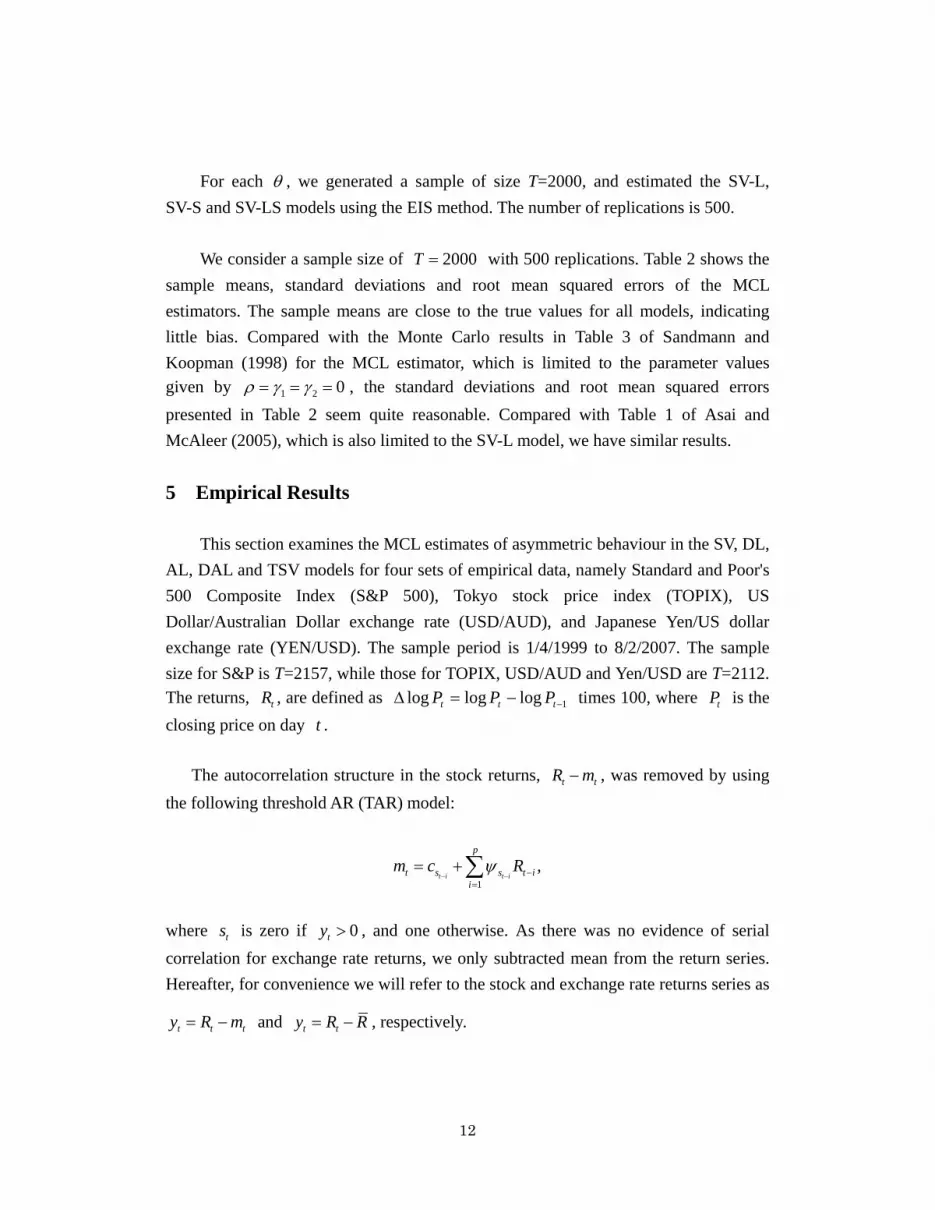
For each θ , we generated a sample of size T=2000, and estimated the SV-L,

SV-S and SV-LS models using the EIS method. The number of replications is 500. We consider a sample size of 2000T = with 500 replications. Table 2 shows the sample means, standard deviations and root mean squared errors of the MCL estimators. The sample means are close to the true values for all models, indicating little bias. Compared with the Monte Carlo results in Table 3 of Sandmann and Koopman (1998) for the MCL estimator, which is limited to the parameter values given by 1 2 0ρ γ γ= = = , the standard deviations and root mean squared errors presented in Table 2 seem quite reasonable. Compared with Table 1 of Asai and McAleer (2005), which is also limited to the SV-L model, we have similar results. 5 Empirical Results

This section examines the MCL estimates of asymmetric behaviour in the SV, DL, AL, DAL and TSV models for four sets of empirical data, namely Standard and Poor's 500 Composite Index (S&P 500), Tokyo stock price index (TOPIX), US Dollar/Australian Dollar exchange rate (USD/AUD), and Japanese Yen/US dollar exchange rate (YEN/USD). The sample period is 1/4/1999 to 8/2/2007. The sample size for S&P is T=2157, while those for TOPIX, USD/AUD and Yen/USD are T=2112. The returns, tR , are defined as 1logloglog −−=Δ ttt PPP times 100, where tP is the closing price on day t . The autocorrelation structure in the stock returns, t tR m− , was removed by using the following threshold AR (TAR) model:

1

,t i t i

p

t s s t ii

m c Rψ− − −

=

= +∑

where ts is zero if 0ty > , and one otherwise. As there was no evidence of serial correlation for exchange rate returns, we only subtracted mean from the return series. Hereafter, for convenience we will refer to the stock and exchange rate returns series as

t t ty R m= − and t ty R R= − , respectively.

13

For stock returns such as S&P 500 and TOPIX, a negative correlation would be expected between the innovations in returns and volatility. Table 3 shows the EIS estimates for S&P 500 returns. Four kinds of SV model were estimated, namely the standard SV model with 1 2 0γ γ= = , SV-L with 2 0γ = , SV-S with 1 0γ = , and SV-LS with no restrictions. The significance of the estimates of 1γ and/or 2γ in the various models leads to a strong rejection of the basic SV model, which neglects the leverage and size effects. The estimates of 1γ in the SV-L and SV-LS model are negative and significant, indicating the existence of the leverage effects. The estimates of 2γ are negative and significant in the SV-S and SV-LS models. AIC and BIC chose the SV-LS model. The likelihood ratio tests favored the SV-LS model.

At this stage, we need to discuss the sign of 2γ . While the estimates of 2γ in the

EGARCH models are always positive in the literature, that for the SV-LS was negative. Our estimates indicate that a negative shock increase volatility, while a positive shock decrease volatility with the different magnitude. This is Case V (Leverage). On the other hand, typical estimates for the EGARCH model imply the Case IV (Standard Asymmetry). As in the EGARCH estimates, it is reasonable that large positive and negative shocks will increase volatility. We need to pay attention to the effect of small positive shock. Recenlty, Chen and Ghysels (2007) found that small positive shock in S&P returns decrease volatility, by their semi-parametric method. This is Case II (General Asymmetry) in our category. However, as the direction of the effect of a small positive shock is different form that of a large positive shock, the SV-LS and EGARCH models are not flexible to capture such effects. If their finding is applicable to our data, the SV-LS model successfully describes the effect of small positive shock, while it fail to capture the effect of large positive shock, which may be absorbed by the innovation term, tη . On the other hand, the EGARCH model may fail to capture the effects of small positive shocks, as it lacks the innovation term.

Table 4 for TOPIX returns shows that the estimates of 1γ are negative and

significant in the SV-L and SV-LS models, but that the estimate of 2γ is insignificant, indicating the rejection of the SV-S model. Both AIC and BIC suggest that SV-L is the best model. The likelihood ratio tests also selected the SV-L. As in the case of S&P 500 returns, the standard SV model is clearly rejected in favour of the two SV models with leverage effects. The size effects may be small so that they are absorbed by the innovation term of volatility.

14

Tables 5 and 6 present the EIS estimates for the USD/AUD and Yen/USD returns, respectively. In Table 5, the results generally lead to similar implications as in the case of the TOPIX returns. AIC, BIC and the likelihood ratio tests also prefer the SV-L model. The estimate of correlation coefficient between the innovations of return and

volatility, 2 21 1ηρ γ σ γ= + , is -0.39 for USD/AUD.

The results for the YEN/USD returns in Table 6 are similar to those for S&P

returns in Table 3. In Tables 6, there is significant evidence of leverage and size effects in the SV-L, SV-S and SV-LS models. The likelihood ratio tests favor the SV-LS model. AIC suggests that the SV-LS is the best model, while BIC chose the SV-S.

Overall, all four estimates indicate that the asymmetric effects for the four

datasets are classified to Case V (Leverage). The slopes of negative and positive shocks are different from each other for the cases of the S&P and YEN/USD returns.

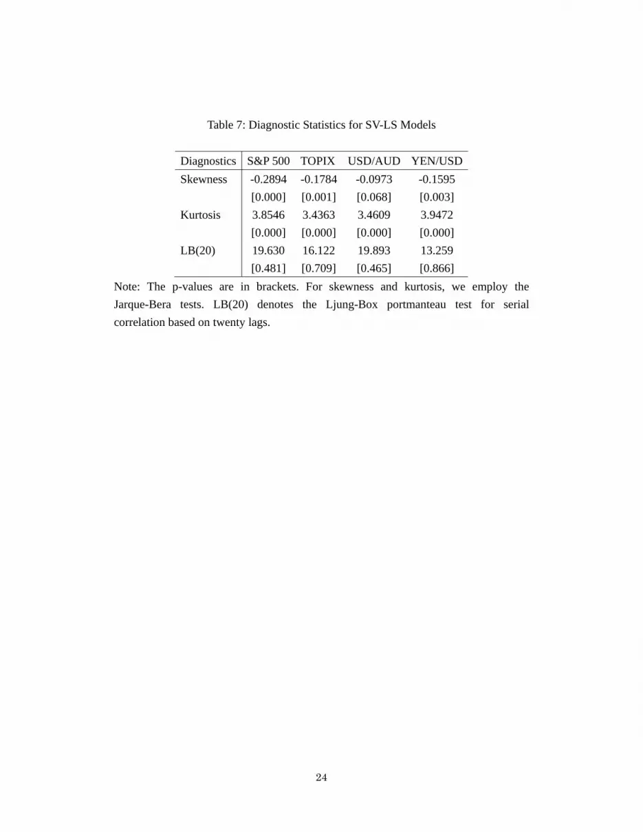
For the diagnostic checking, we calculated filtered estimates of volatility,

( ) 1exp t tE h y −⎡ ⎤⎣ ⎦ , t=1,2,…,T. Table 7 shows the diagnostic statistics for the

standardized residuals. For all four series, we have the same results as follows. The Ljung-Box portmanteau tests based on twenty lags support no serial correlation. The Jarque-Bera tests reject the null of normal distribution. In order to consider the heavy-tailed conditional distribution, we estimated the SV-t-LS model. Table 8(a) presents the parameter estimates of the SV-t-LS model for four series. For all series except for YEN/USD, the estimates of 1 v are close to zero and insignificant, which may be caused by misspecification of the structure of asymmetry and/or tail-behavior. With respect to YEN/USD, the estimate of 1γ is negative and significant while that of 2γ is positive and significant. Compared to the estimates of SV-LS in Table 6, the sign of 2γ is changed. The estimate of 1 v is significant, and the estimate of v is 6.33. Table 8(b) shows the log-likelihood, AIC and BIC. For the case of YEN/USD, the likelihood ratio test shows that 1 v is significant, while the model has the smallest AIC and BIC. For the other three series, AIC and BIC shows that there is no improvement form introducing the heavy-tailed conditional distribution. Table 8(c) shows the diagnostic statistics for the standardized residuals. The Ljung-Box portmanteau tests based on twenty lags support no serial correlation for

15

all series. We employed the test proposed by Godfrey and Orme (1991) for asymmetry under heavy-tailed distributions. The test does not reject the null of symmetry except for TOPIX. The test for excess kurtosis rejects the null for YEN/USD, as expected from the t distribution. 6 Conclusion In this paper, we suggested a new asymmetric stochastic volatility model, based on the leverage and size effects, as an extension of the EGARCH model. We considered five categories for asymmetric effects, which describes the difference among the asymmetric effect of the EGARCH model, the threshold effects of GJR model, and the leverage effects of SV model. We consider the SV with leverage effects (SV-L), the SV with size effect (SV-S), and the general asymmetric SV model (SV-LS). These three models are estimated by the efficient importance sampling method of Liesenfeld and Richard (2003), and the finite sample properties of the estimator are investigated using Monte Carlo experiments. We used four financial time series are used to estimate the alternative asymmetric SV models. The empirical results for S&P 500 and Yen/USD returns preferred the SV-LS model, while TOPIX and USD/AUD returns favored the SV-L model. For the case of standardized t distribution, the results for Yen/USD returns show that the model is correctly specified, while the results for three other data sets suggested there was scope for improvement. In addition to providing more accurate estimates of volatility, these empirical results should assist in calculating optimal Value-at-Risk (VaR) forecasts and capital charges for purposes of portfolio and risk management.

This paper has made certain contributions, but several extensions are still possible. First, we may work with multi-factors as in Chernov et al. (2003) and Asai (2008), in order to capture tail behavior. Secondly, we may consider more flexible specifications of asymmetry, which describe the results of Chen and Ghysels (2007). Thirdly, the paper focuses on leptokurtic distribution, but it is also worthwhile fitting skewed distributions, including the skewed t distribution (Fernández and Steel (1998)).

16

References Asai, M. (2005), “Comparison of MCMC Methods for Estimating Stochastic Volatility

Models”, Computational Economics, 25, 281-301. Asai, M. (2008), “Autoregressive Stochastic Volatility Models with Heavy-Tailed

Distributions: A Comparison with Multifactor Volatility Models”, Journal of Empirical Finance, 15, 332-341.

Asai, M. and M. McAleer (2005), “Dynamic Asymmetric Leverage in Stochastic

Volatility Models”, Econometric Reviews, 24, 317-332. Black, F. (1976), “Studies of Stock Market Volatility Changes”, 1976 Proceedings of

the American Statistical Association, Business and Economic Statistics Section, pp. 177-181.

Bollerslev, T., R.Y. Chou and K.F. Kroner (1992), “ARCH Modelling in Finance: A

Review of the Theory and Empirical Evidence”, Journal of Econometrics, 52, 5-59.

Bollerslev, T., R.F. Engle and D.B. Nelson (1994), “ARCH Models”, in R.F. Engle and

D. McFadden (eds.), Handbook of Econometrics, 4, North-Holland, Amsterdam, pp. 2961-3038.

Bollerslev, T. and H. Zhou (2006), “Volatility Puzzles: A Simple Framework for

Gauging Return-Volatility Regressions”, Journal of Econometrics, 131,123-150. Chen, X. and E. Ghysels (2007), “News - Good or Bad - and its Impact Over Multiple

Horizons”, Unpublished paper, Department of Economics, University of North Carolina at Chapel Hill.

Chernov, M., A.R. Gallant, E. Ghysels, and G. Tauchen (2003), “Alternative Models

for Stock Price Dynamics”, Journal of Econometrics, 116, 225–257. Chesney, M. and L.O. Scott (1989), “Pricing European Currency Options: A

Comparison of the Modified Black-Scholes Model and a Random Variance

17

Model”, Journal of Financial and Quantitative Analysis, 24, 267-284. Chib, S., F. Nardari and N. Shephard (2002), “Markov Chain Monte Carlo Methods for

Stochastic Volatility Models”, Journal of Econometrics, 108, 281-316. Christie, A.A. (1982), “The Stochastic Behavior of Common Stock Variances: Value,

Leverage and Interest Rate Effects”, Journal of Financial Economics, 10, 407-432.

Engle, R.F. (1982), “Autoregressive Conditional Heteroskedasticity with Estimates of

the Variance of United Kingdom Inflation”, Econometrica, 50, 987-1007. Fernández, C., and M.F.J. Steel (1998), “On Bayesian Modeling of Fat Tails and

Skewness”, Journal of the American Statistical Association, 93, 359–371. French, K., G.W. Schwert and R. Stambaugh (1987), “Expected Stock Returns and

Volatility”, Journal of Financial Economics, 19, 3-29. Fridman, M. and L. Harris (1998), “A Maximum Likelihood Approach for

Non-Gaussian Stochastic Volatility Models”, Journal of Business and Economic Statistics, 16, 284-291.

Gallant, A.R. and G. Tauchen (1989), “Seminonparametric Estimation of Conditional

Constrained Heterogeneous Processes: Asset Pricing Applications”, Econometrica, 57, 1091-1120.

Gallant, A.R., D.A. Hsieh and G. Tauchen (1991), “On Fitting a Recalcitrant Series: the

Pound/Dollar Exchange Rate, 1974-83”, in W.A. Barnett, J. Powell, and G. Tauchen (eds.), Nonparametric and Semiparametric Methods in Econometrics and Statistics, Proceedings of the Fifth International Symposium in Economic Theory and Econometrics, Cambridge University Press, Cambridge, pp. 199-240.

Geweke, J. (1992), “Evaluating the Accuracy of Sampling-Based Approaches to the

Calculation of Posterior Moments”, in J.M. Bernardo, J.O. Berger, A.P. Dawid and A.F.M. Smith (eds.), Bayesian Statistics 4, Oxford University Press, Oxford, pp.169-193.

18

Glosten, L., R. Jagannathan and D. Runkle (1992), “On the Relation Between the

Expected Value and Volatility of Nominal Excess Returns on Stocks”, Journal of Finance, 46, 1779-1801.

Godfrey, L. G. and C.D. Orme (1991), “Testing for Skewness of Regression

Disturbances”, Economics Letters, 37, 31–34. Harvey, A.C. and N. Shephard (1996), “Estimation of an Asymmetric Stochastic

Volatility Model for Asset Returns”, Journal of Business and Economic Statistics, 14, 429-434.

Hentschel, L. (1995), “All in the Family: Nesting Symmetric and Asymmetric GARCH

Models”, Journal of Financial Economics, 39, 71-104. Hull, J. and A. White (1987), “The Pricing of Options on Assets with Stochastic

Volatility”, Journal of Finance, 42, 281-300. Jacquier, E., N.G. Polson and P.E. Rossi (1994), “Bayesian Analysis of Stochastic

Volatility Models”, Journal of Business and Economic Statistics, 12, 371-389. Jacquier, E., N.G. Polson and P.E. Rossi (2004), “Bayesian Analysis of Stochastic

Volatility Models with Fat-tails and Correlated Errors”, Journal of Econometrics, 122, 185-212.

Liesenfeld, R., and J.-F. Richard (2003), “Univariate and Multivariate Stochastic

Volatility Models: Estimation and Diagnostics”, Journal of Empirical Finance, 10, 505-531.

Ling, S. and M. McAleer (2000), “Testing GARCH Versus EGARCH”, in W.-S. Chan,

W.K. Li and H. Tong (eds.), Statistics and Finance: An Interface, Imperial College Press, London, pp. 226-242.

McAleer, M. (2005), “Automated Inference and Learning in Modeling Financial

Volatility”, Econometric Theory, 21, 232-261.

19

McAleer, M., F. Chan and D. Marinova (2007), “An Econometric Analysis of Asymmetric Volatility: Theory and Application to Patents”, Journal of Econometrics, 139, 259-284.

Nelson, D.B. (1991), “Conditional Heteroskedasticity in Asset Returns: A New

Approach”, Econometrica, 59, 347-370. Omori, Y., S. Chib, N. Shephard and J. Nakajima (2007), “Stochastic Volatility with

Leverage: Fast and Efficient Likelihood Inference”, Journal of Econometrics, 140, 425-449.

Pagan, A. and G.W. Schwert (1990), “Alternative Models for Conditional Stock

Volatility”, Journal of Econometrics, 45, 267-290. Sandmann, G.. and S.J. Koopman (1998), “Estimation of Stochastic Volatility

ModeSV-Lia Monte Carlo Maximum Likelihood”, Journal of Econometrics, 87, 271-301.

Shephard, N. and M.K. Pitt (1997), “Likelihood Analysis of Non-Gaussian

Measurement Time Series”, Biometrika, 84, 653-667. So, M.K.P., W.K. Li and K. Lam (2002), “A Threshold Stochastic Volatility Model”,

Journal of Forecasting, 21, 473-500. Taylor, S.J. (1986), Modelling Financial Time Series, Wiley, Chichester. Wiggins, J.B. (1987), “Option Values Under Stochastic Volatility: Theory and

Empirical Estimates”, Journal of Financial Economics, 19, 351-372. Yu, J. (2005), “On Leverage in a Stochastic Volatility Model”, Journal of Econometrics,

127, 165-178.

20

Table 1: Parametric Restrictions for Symmetry, Asymmetry and Leverage

Model Case I

Symmetry Case II General

Asymmetry

Case III Wide

Asymmetry

Case IV Standard

Asymmetry

Case V Leverage

GJR 0,0

αγ>=

NA 0,

,0

αγ αγ

>> −≠

0,0

αγ>>

NA

EGARCH 0,0

λθ≠=

θ λ< ,

0θ λθ

<

≠

0,θλ θ<> −

0,θ

λ θ<

< −

SV-L NA NA NA NA 1 0γ <

SV-S 2 0γ ≠ NA NA NA NA

SV-LS 1

2

0,0

γγ=≠

1 2γ γ< 1

1 2

0,γγ γ≠

< 1

2 1

0,γγ γ<> −

1

2 1

0,γγ γ<

< −

Note: NA denotes not applicable.

21

Table 2: Finite Sample Performance of the EIS Estimator for T=2000

Parameter SV-L SV-S SV-LS

μ 0.0074 0.0168 0.0193 (0.1074) (0.1158) (0.1686) [0.1076] [0.1170] [0.1697]φ 0.9477 0.9466 0.9467 (0.0112) (0.0126) (0.0125) [0.0115] [0.0131] [0.0129]

ησ 0.2228 0.2117 0.1974

(0.0334) (0.0330) (0.0801) [0.0334] [0.0331] [0.0801]

1γ -0.0802 -0.0817 (0.0380) (0.0249) [0.0380] [0.0249]

2γ 0.1655 0.1653 (0.0628) (0.0571) [0.0630] [0.0573]

Note: Standard errors are in parentheses and root mean squared errors are in brackets. True parameters are 0μ = , 0.95φ = , and

( ) ( ) ( ) ( ){ }1 2, , 0.222, 0.08,0 , 0.215,0,0.16 , 0.200, 0.08,0.16ησ γ γ = − − ,

corresponding to the SV-L, SV-L and SV-LS models, respectively.

22

Table 3: EIS Estimates for S&P 500 Returns

Model φ ησ μ 1γ 2γ LogLike AIC BIC

SV 0.9914 0.1048 -0.0751 -2993.45 5992.90 6009.93 (0.0035) (0.0153) (0.2536)

SV-L 0.9842 0.0718 -0.1398 -0.1191 -2943.84 5895.69 5918.39 (0.0031) (0.0115) (0.1048) (0.0133)

SV-S 0.9943 0.0722 -0.1870 -0.1130 -2990.72 5989.43 6012.14 (0.0032) (0.0360) (0.3257) (0.0535)

SV-LS 0.9901 0.0104 -0.1624 -0.1140 -0.1282 -2937.35 5884.79 5913.08 (0.0020) (0.0032) (0.1324) (0.0116) (0.0197)

Note: Standard errors are given in parentheses.

Table 4: EIS Estimates for TOPIX Returns

Model φ ησ μ 1γ 2γ LogLike AIC BIC

SV 0.9714 0.1463 0.2111 -3308.10 6622.20 6639.16 (0.0084) (0.0203) (0.1146)

SV-L 0.9492 0.1706 0.2051 -0.1108 -3288.38 6584.77 6607.39 (0.0118) (0.0226) (0.0800) (0.0207)

SV-S 0.9735 0.1436 0.1815 -0.0522 -3307.57 6623.13 6645.75 (0.0082) (0.0214) (0.1197) (0.0514)

SV-LS 0.9522 0.1707 0.1817 -0.1127 -0.0748 -3287.36 6584.71 6612.99 (0.0112) (0.0233) (0.0804) (0.0207) (0.0531)

Note: Standard errors are given in parentheses.

23

Table 5: EIS Estimates for USD/AUD Returns

Model φ ησ μ 1γ 2γ LogLike AIC BIC

SV 0.9699 0.1322 0.5144 -3609.77 7225.55 7242.52 (0.0096) (0.0212) (0.0997)

SV-L 0.9619 0.1431 0.5034 -0.0598 -3601.54 7211.09 7233.71 (0.0108) (0.0213) (0.0875) (0.0161)

SV-S 0.9717 0.1311 0.4986 -0.0417 -3609.40 7226.80 7249.42 (0.0094) (0.0222) (0.1017) (0.0486)

SV-LS 0.9624 0.1462 0.4890 -0.0607 -0.0428 -3601.15 7212.30 7240.57 (0.0110) (0.0224) (0.0871) (0.0163) (0.0493)

Note: Standard errors are given in parentheses.

Table 6: EIS Estimates for YEN/USD Returns

Model φ ησ μ 1γ 2γ LogLike AIC BIC

SV 0.9667 0.1496 -1.1207 -1877.46 3760.93 3777.90 (0.0121) (0.0282) (0.1027)

SV-L 0.9636 0.1501 -1.1200 -0.0377 -1874.64 3757.28 3779.91 (0.0124) (0.0281) (0.0954) (0.0165)

SV-S 0.9684 0.1548 -1.2635 -0.1320 -1871.71 3751.42 3774.05 (0.0115) (0.0311) (0.1164) (0.0440)

SV-LS 0.9675 0.1501 -1.2634 -0.0386 -0.1382 -1868.62 3747.24 3775.52 (0.0113) (0.0309) (0.1118) (0.0158) (0.0447)

Note: Standard errors are given in parentheses.

24

Table 7: Diagnostic Statistics for SV-LS Models

Diagnostics S&P 500 TOPIX USD/AUD YEN/USD Skewness -0.2894 -0.1784 -0.0973 -0.1595 [0.000] [0.001] [0.068] [0.003] Kurtosis 3.8546 3.4363 3.4609 3.9472 [0.000] [0.000] [0.000] [0.000] LB(20) 19.630 16.122 19.893 13.259 [0.481] [0.709] [0.465] [0.866]

Note: The p-values are in brackets. For skewness and kurtosis, we employ the Jarque-Bera tests. LB(20) denotes the Ljung-Box portmanteau test for serial correlation based on twenty lags.

25

Table 8: EIS Estimates for SV-t-LS Models

(a) Paramter Estimates

Model φ ησ μ 1γ 2γ 1 v

S&P 500 0.9900 0.0162 -0.1628 -0.1141 -0.1263 2.52 510−× (0.0020) (0.0057) (0.1372) (0.0117) (0.0182) (0.0053)

TOPIX 0.9522 0.1707 0.1820 -0.1126 -0.0748 3.93 510−× (0.0113) (0.0234) (0.0804) (0.0208) (0.0532) (0.0020)

USD/AUD 0.9635 0.1441 0.4888 -0.0600 -0.0434 5.38 510−× (0.0107) (0.0222) (0.0884) (0.0162) (0.0500) (0.0066)

YEN/USD 0.9808 0.0695 -1.0129 -0.0304 0.0663 0.1580 (0.0073) (0.0190) (0.1456) (0.0149) (0.0275) (0.0362)

Note: Standard errors are given in parentheses.

(b) Log-Likelihood and Information Criterions Model LogLike AIC BIC

S&P 500 -2937.35 5886.76 5920.78TOPIX -3287.36 6586.72 6620.65

USD/AUD -3601.14 7214.28 7248.22YEN/USD -1852.78 3717.55 3751.48

(c) Diagnostic Statistics

Diagnostics S&P 500 TOPIX USD/AUD YEN/USD Skewness -0.2242 -0.2205 -0.1435 -0.1947 [0.075] [0.029] [0.121] [0.078] Kurtosis 4.2437 3.9706 3.7652 4.1848 [0.000] [0.000] [0.000] [0.000] LB(20) 22.753 16.219 20.573 13.029 [0.301] [0.703] [0.423] [0.876]

Note: The p-values are in brackets. We employ the Jarque-Bera test for excess kurtosis. With respect to skewness, we use the test proposed by Godfrey and Orme (1991) for asymmetry under heavy-tailed distributions. LB(20) denotes the Ljung-Box portmanteau test for serial correlation based on twenty lags.