Embed Size (px)
Citation preview

High frequency volatility of volatility
estimation free from spot volatility
estimates
Simona Sanfelici∗, Imma Valentina Curato†and Maria Elvira Mancino‡
Abstract
We define a new consistent estimator of the integrated volatility of volatilitybased only on a pre-estimation of the Fourier coefficients of the volatility process.We investigate the finite sample properties of the estimator in the presence of noisecontamination by computing the bias of the estimator due to noise and showing thatit vanishes as the number of observations increases, under suitable assumptions.In both simulated and empirical studies, the performance of the Fourier estimatorwith high frequency data is investigated and it is shown that the proposed estimatorof volatility of volatility is easily implementable, computationally stable and evenrobust to market microstructure noise.
Keywords: stochastic volatility, volatility of volatility, high frequency data, microstruc-
ture, Fourier analysis
JEL classification: C13, C22
1 Introduction
Motivated by empirical studies showing the patterns of volatilities in financial time series,
in the last decades many stochastic volatility models have been proposed: such mod-
els are able to reproduce some stylized facts as variance heteroscedasticity, predictabil-
ity, volatility smile, negative correlation between asset returns and volatility; very re-
cently, [Barndorff-Nielsen and Veraart, 2013] propose a new class of stochastic volatility
∗University of Parma, Italy - E-mail: [email protected]†Ulm University, Germany - E-mail: [email protected]‡University of Florence, Italy - E-mail: [email protected]
1

of volatility models, introducing an extra source of randomness. The estimation of all
these models is rather complicated, the main difficulties are due to the fact that some
factors are unobservable (e.g. the volatility in a standard stochastic volatility model or
even more, the stochastic volatility of volatility in the stochastic volatility of volatility
models), thus we have to handle them as latent variables.
In this paper, we focus on the estimation of integrated stochastic volatility of volatility us-
ing high frequency data and we define a consistent non parametric estimator based on the
Fourier series methodology introduced in [Malliavin and Mancino, 2002, Malliavin and Mancino, 2009],
which works both in the case of classical stochastic volatility models and in the context
of stochastic volatility of volatility models. The proposed estimator needs only to pre-
estimate the Fourier coefficients of the volatility process from the observations of a price
process and does not require a preliminary estimation of the instantaneous volatility.
An early application of the Fourier methodology to identify the parameters (volatility
of volatility and leverage, i.e., the covariance between the stochastic variance process
and the asset price process) of stochastic volatility models, including classical models
such as [Heston, 1993, Hull and White, 1987, Stein and Stein, 1991], has been developed
in [Barucci and Mancino, 2010]. However, the problem of robustness with respect to
microstructure noise is not addressed by the authors; hence, the numerical simulations
assessing the performance of the method employ low frequency observations.
The issue of estimating the volatility of volatility in the presence of jumps is studied in
[Cuchiero and Teichmann, 2013]: firstly the authors combine jump robust estimators of
integrated realized variance and the Fourier-Fejer inversion formula to get an estimator
of the instantaneous volatility path; secondly they use again jump robust estimators for
integrated volatility in which they plug the estimated path of the volatility process in order
to obtain an estimator of the volatility of volatility. [Barndorff-Nielsen and Veraart, 2013]
define a class of stochastic volatility of volatility models and show that it can be estimated
non-parametrically by means of the quadratic variation of the preliminarly estimated
squared volatility process, which they name pre-estimated spot variance based realised
variance. [Vetter, 2011] proposes an estimator for the integrated volatility of volatility,
which is also based on increments of the pre-estimated spot volatility process and attains
the optimal convergence rate. The common feature of these estimators is that they first
estimate the volatility path using some consistent estimate of the instantaneous volatility;
secondly, they estimate the volatility of volatility using the estimated volatility process
as a proxy of the unknown paths. However these estimators do not take into account the
microstructure noise effects, which would seriously affect the accuracy of the estimation
as the spot volatility estimators are quite sensitive to noise.
In the present work we define the Fourier estimator of volatility of volatility, we prove
2

its consistency and we claim the efficiency of our method when applied to compute the
volatility of the volatility in the presence of microstructure noise. To this end, we compute
the bias due to noise of the proposed estimator of volatility of volatility and we show
that it converges to zero, as the number of observations increases, by suitably cutting the
highest frequencies in the Fourier expansions. This result is due to the intrinsic robustness
of the Fourier estimator of volatility; in fact, the finite sample properties of the Fourier
estimator of integrated volatility in the presence of market microstructure noise have been
studied in [Mancino and Sanfelici, 2008], where the authors find that, even without any
bias correction of the estimator, the bias of a finite sample can be made negligible by
suitably cutting the highest frequencies in the Fourier expansion. Our procedure can be
extended without any conceptual difficulties to the multidimensional setting.
We stress the point that the Fourier estimator of the volatility of volatility is notably
different from the other proposed volatility of volatility estimators: in fact, they all use
some estimated instantaneous volatility path in order to define the volatility of volatility
estimators by means of some numerical differentiation (more or less in spirit they are
quadratic or power variation of the estimated spot volatilities). On the contrary, our ap-
proach relies only on integrated quantities, i.e. the Fourier coefficients of the volatility. As
it was early observed in [Malliavin and Mancino, 2002], this is a peculiarity of the Fourier
estimator that renders the proposed method easily implementable, computationally stable
and even robust to market microstructure noise.
The finite sample performance of the Fourier estimator of volatility of volatility is tested
in extensive numerical simulations, using both classical stochastic volatility models, where
the spot variance follows a mean-reverting square-root process, and models with stochas-
tic volatility of volatility, namely where the volatility of the variance process is driven
by a second source of randomness. Our analysis is threefold. We first show the sen-
sitivity of the Fourier estimator to the choice of the cutting frequencies, to which the
consistency of the estimator is related, and we test the robustness of the estimator with
respect to several noise settings. Then, we test the performance of the Fourier esti-
mator using as a benchmark the pre-estimated spot variance based realised variance of
[Barndorff-Nielsen and Veraart, 2013] and the bias corrected realized variance estimator
of [Vetter, 2011]. Finally, we address the issue of parameter identification of stochastic
volatility models and we consider an empirical application to S&P 500 index futures.
The paper is organized as follows. Section 2 reviews the Fourier methodology for esti-
mating volatilities. In Section 3, we define the Fourier estimator of volatility of volatility
and prove its consistency. The asymptotically unbiasedness of the estimator with respect
to (some kind of) microstructure noise is proved in Section 4. In Section 5, we test its
3

performance in several scenarios. Section 6 concludes. The technical proofs are contained
in the Appendix.
2 The Fourier method for computing volatilities
We consider a fairly general class of stochastic volatility models. Suppose that the log
price-variance processes satisfy
(A.I)
dp(t) = σ(t)dW (t) + a(t)dt
dv(t) = γ(t)dZ(t) + b(t)dt
where p(t) is the logarithm of the asset price and v(t) := σ2(t) is the variance process. Let
W and Z be correlated Brownian motions on a filtered probability space (Ω, (Ft)t∈[0,T ], P ),
satisfying the usual conditions. Assume that σ(t), γ(t) are non-negative adapted processes
and a(t), b(t) are adapted processes such that
(A.II)
E[∫ T
0a2(t)dt] <∞, E[
∫ T0b2(t)dt] <∞
E[∫ T
0σ4(t)dt] <∞, E[
∫ T0γ4(t)dt] <∞.
Therefore our stochastic volatility models assume the variance process to be a continuous
Brownian semimartingale, but the volatility of the variance process might have jumps.
Further, we will show in Section 5 that the proposed estimator of volatility of volatility
works well also in the stochastic volatility of volatility models by [Barndorff-Nielsen and Veraart, 2013].
In the sequel we will often refer to the process v(t) as the volatility, as it is usually done
in the econometric literature.
We briefly recall the Fourier volatility estimation method by [Malliavin and Mancino, 2009].
By rescaling the unit of time, we can always reduce ourselves to the case where the time
window [0, T ] becomes [0, 2π]. Then, define the k-th Fourier coefficient of the price process
ck(dp) :=1
2π
∫ 2π
0
exp(−ikt) dp(t) ,
and consider for all integers k the Bohr convolution product
limN→∞
2π
2N + 1
∑|s|≤N
cs(dp)ck−s(dp). (1)
In [Malliavin and Mancino, 2009] it is proved that the limit (1) exists in probability and
it is equal to the k-th Fourier coefficient of the volatility process v, which we denote as
ck(v).
4

The knowledge of the Fourier coefficients ck(v) of the unobservable instantaneous volatility
process v(t) allows to handle this process as an observable variable and we can iterate
the procedure in order to compute the volatility of the volatility process: given the price-
variance model in (A.I), the k-th Fourier coefficient of the volatility γ2(t) of the volatility
process can be computed as the following limit in probability
ck(γ2) = lim
M→∞
2π
2M + 1
∑|s|≤M
cs(dv)ck−s(dv), (2)
where we can use the integration by parts formula to write the Fourier coefficients of dv,
that is, for any integer k, k 6= 0,
ck(dv) = ikck(v) +1
2π(v(2π)− v(0)).
We start from this key property of Fourier estimation method, namely the possibility of
iterating the Bohr convolution procedure, and we propose an estimator of the integrated
volatility of volatility, indeed the zero Fourier coefficient of the process γ2(t), which is
easily implementable with high frequency market data.
The idea of using the estimated Fourier coefficients of the volatility as building blocks to
obtain results for other related quantities has been applied in [Malliavin and Mancino, 2002a]
to compute the price-volatility feedback-rate, in [Mancino and Sanfelici, 2012] to estimate
the quarticity and in [Curato and Sanfelici, 2014] for the estimation of the leverage, i.e.,
the covariance between the stochastic variance process and the asset price process.
In this paper, we claim the effectiveness of Fourier estimation method when applied to
compute the volatility of the volatility in the presence of microstructure noise, a result
that is due to the intrinsic robustness of the Fourier estimator of volatility. In fact,
[Mancino and Sanfelici, 2008] analyse the finite sample properties of the Fourier estimator
of integrated volatility in the presence of market microstructure noise and find out that,
even without any bias correction of the estimator, the bias on a finite sample can be
made negligible by suitably cutting the highest frequencies in the Fourier expansion. In
this paper, we analytically compute the bias of the Fourier estimator of the volatility
of volatility due to the presence of noise and we show that this bias is asymptotically
vanishing, under a suitable choice of the number of Fourier frequencies.
3 The Fourier estimator of volatility of volatility
In this section we define the Fourier estimator of the volatility of volatility which relies on
the convolution formulae (1) and (2); then we prove that it is consistent in probability.
5

For any positive integer n, let Sn := 0 = t0 ≤ · · · ≤ tn = 2π be the set of (possibly
unequally-spaced) trading dates of the asset, i.e., the observation times of the asset price.
Denote ρ(n) := max0≤i≤n−1 |ti+1 − ti| and suppose that ρ(n) → 0 as n → ∞. Moreover,
let δi(p) := p(ti+1)− p(ti).For any integer k, |k| ≤ 2N , let
ck(dpn) :=1
2π
n−1∑i=0
exp(−ikti)δi(p), (3)
then for any integer j, |j| ≤ N , let
cj(vn,N) :=2π
2N + 1
∑|k|≤N
ck(dpn)cj−k(dpn). (4)
The following result states the consistency of the estimator (4) of the Fourier coefficients
of the volatility process. The proof can be found in [Malliavin and Mancino, 2009].
Theorem 3.1 Under the assumptions (A.I) and (A.II) and the condition ρ(n)N → 0,
then, for any integer j, the following convergence in probability holds
limn,N→∞
cj(vn,N) = cj(v).
Given the estimated Fourier coefficients of the volatility process (4), we construct an
estimator of the second order quantity (i.e. the volatility of volatility) starting from (2).
More precisely, we define the Fourier estimator of the (integrated) volatility of volatility∫ 2π
0γ2(t)dt as
γ2n,N,M :=
(2π)2
M + 1
∑|j|≤M
(1− |j|
M
)j2 cj(vn,N)c−j(vn,N). (5)
In (5) we have chosen to add a Barlett kernel, which improves the behavior of the estimator
for very high observation frequencies.
We emphasize the fact that the estimator (5) does not require the preliminary estimation
of the instantaneous volatility, but only the estimated Fourier coefficients of the volatility.
As far as we know, all the recently proposed estimators of volatility of volatility need the
estimated volatility path in order to estimate the volatility of volatility, the ratio being that
the reconstructed (estimated) path of the volatility is plugged into an estimator of inte-
grated volatility, e.g. the realized volatility (see, for instance, [Barndorff-Nielsen and Veraart, 2013,
Cuchiero and Teichmann, 2013, Vetter, 2011]). Therefore a large number of observations
for the price process is necessary, as it is statistically clear that the integrated variance
6

of the volatility process can be estimated only on a larger time scale than the one used
for estimating the volatility path from the observed prices. This yields a huge loss of
information contained in the original dataset. On the other side, it is well known that
spot volatility estimation is quite unstable, especially in the presence of microstructure
effects as it happens with high frequency data. On the contrary, the Fourier estimator can
reconstruct the integrated volatility of volatility using as input the Fourier coefficients of
the observable log-returns, in other words using only integrated quantities from the whole
dataset.
In order to prove the consistency of the proposed estimator we add a further assumption
on the values of the volatility at the end points (see [Barndorff-Nielsen and al., 2008] for
a similar idea):
(A.III) we redefine the two end values v(0) and v(2π) to be respectively equal tov(0+)+v(0−)
2and v(2π+)+v(2π−)
2. Equivalently, we can use an average of m distinct obser-
vations in the intervals (−ε, ε) and (2π − ε, 2π + ε). This jittering is used to eliminate
end-effects that would otherwise appear.
The following result proves that (5) is a consistent estimator of the integrated volatility
of volatility and gives the growth rates between the highest Fourier frequencies N and M ,
which are needed for the construction of the estimators cj(vn,N) and γ2n,N,M , respectively,
and the initial mesh width ρ(n) of the price process observations.
Theorem 3.2 Under the assumptions (A.I), (A.II), (A.III) and the conditions Nρ(n)→0 and M4
N→ 0, then the following convergence in probability holds
limn,N,M→∞
γ2n,N,M =
∫ 2π
0
γ2(t)dt.
Remark 3.3 The multivariate extension of our results to obtain a high frequency estima-
tor of the covariance of the covariance matrix is essentially contained in the proposed the-
ory. In fact, the Fourier method was originally introduced by [Malliavin and Mancino, 2002]
for the estimation of multivariate volatility in order to overcome the difficulties intrinsic
in the use of the quadratic covariation formula on true return data, due to the non-
synchronicity of observed prices on different assets. We do not intend to develop this
theory in the present paper, but we claim that the availability of a multivariate extension
is an added important advantage of our estimator of second order quantities.
4 Robustness to microstructure noise
In this section we derive the analytical expression of the bias of the Fourier estimator of
volatility of volatility due to the presence of microstructure noise, for a given sample size
7

n and a given number of Fourier coefficients N and M included in the estimation and we
prove that the bias of the Fourier estimator converges to zero, for n,N,M increasing at
suitable rates. Therefore, even if we do not proceed to any bias correction of the estimator,
a suitable cutting of the highest frequencies can make the finite sample bias negligible.
We suppose that the logarithm of the observed price process is given by
p(t) = p(t) + η(t) (6)
where p(t) is the efficient log price in equilibrium and η(t) is the microstructure noise.
The following assumptions hold:
(M.I) the random shocks η(ti)0≤i≤n, for all n, are independent and identically dis-
tributed with mean zero and bounded fourth moment;
(M.II) the shocks η(ti)0≤i≤n are independent of the price process p, for all n.
Remark 4.1 We consider here the simple case where the microstructure noise displays
an MA(1) structure with a negative first-order autocorrelation. The MA(1) model is typ-
ically justified by bid-ask bounce effects [Roll, 1984]. The hypothesis that the random
noises are independent of the returns (see the discussion in [Hansen and Lunde, 2006]) is
assumed here with the aim to obtain simple analytic expressions for the bias. Nevertheless,
we expect that similar results would be observed under more general microstructure noise
dependence, as a consequence of the robustness of volatility Fourier estimator proved in
[Mancino and Sanfelici, 2008] under general dependent noise structure. A specific simu-
lation study confirming this intuition is developed in Section 5.
To simplify the notation, in the sequel we will write ηi instead of η(ti). Denote δi(p) :=
p(ti+1)− p(ti), where p is defined in (6). Then δi(p) = δi(p) + εi, where εi := ηi+1 − ηi.We focus on the estimator of integrated volatility of volatility in the presence of mi-
crostructure noise defined by:
γ2n,M,N =
(2π)2
M + 1
∑|j|≤M
(1− |j|M
)j2 cj(vn,N)c−j(vn,N) (7)
where
cj(vn,N) =2π
2N + 1
∑|k|≤N
ck(dpn)cj−k(dpn),
is the estimated j-th Fourier coefficient of the volatility, given price observations contam-
inated by microstructure noise.
The following result contains the computation of the bias induced by the noise. For
simplicity we assume equally spaced data in the following theorem.
8

Theorem 4.2 Under the assumptions (A.I), (A.II) and (M.I), (M.II), let γ2n,M,N and
γ2n,M,N be defined respectively by (5) and (7). Then, it holds
E[γ2n,M,N − γ2
n,M,N ]
= 2E[η2]E[
∫ 2π
0
σ2(t)dt] Λ(n,N,M) + 2(E[η4] + 3E[η2])Γ(n,N,M) + 2E[η2]Ψ(n,N,M),
where Λ(n,N,M), Γ(n,N,M) and Ψ(n,N,M) are deterministic functions which go to 0
as n,N,M →∞, under the conditions M2N2
n→ 0 and M2
N→ 0.
Remark 4.3 From Theorem 3.2 and Theorem 4.2, the growth conditions ensuring both
the consistency of the Fourier estimator of volatility of volatility (7) and its asymptotically
unbiasedness in the presence of microstructure noise are that N = O(nα) and M = O(nβ)
with 0 < α < 12
and 0 < β < α4
.
5 Numerical results
In this section, we simulate discrete data from a continuous time stochastic volatil-
ity model with and without microstructure contaminations. From the simulated data,
Fourier estimates of the integrated volatility of volatility can be compared to the value
of the true quantity and to estimates obtained with other methods proposed in the
literature. However, to the best of our knowledge, only very recently the literature
has been focused specifically on the analysis of estimators for integrated volatility of
volatility. We refer to the works of [Barndorff-Nielsen and Veraart, 2013, Vetter, 2011,
Cuchiero and Teichmann, 2013]. None of these contributions, however, consider the issue
of microstructure effects which may be problematic in empirical applications and therefore
they do not apply to a real high frequency setting.
Another aspect that is worth mentioning is that, by their nature, all existing estimators of
volatility of volatility rely on a preliminary estimation of the spot volatility path. It is well
known that spot volatility estimation is particularly difficult and quite unstable, especially
in the presence of microstructure effects. On the contrary, the Fourier estimator can
reconstruct the Fourier coefficients of the volatility of the variance process starting from
the observable log-prices. Therefore, our estimate is obtained by iterated convolutions
of the Fourier coefficients of the log-returns, without resorting explicitly to any proxy of
the latent spot variance of returns. We think that this can represent a strength of our
approach, as it will be highlighted by the following numerical simulations.
As a benchmark for our estimator, we use the pre-estimated spot variance based realised
variance of [Barndorff-Nielsen and Veraart, 2013], which we call realised variance in the
9

following. This estimator is consistent in the absence of microstructure frictions. To
obtain roughly unbiased and valid estimates of the integrated volatility of volatility when
microstructure effects play a role, we can resort to low frequency sampling. However, the
well known bias-variance trade off comes up as sparse sampling eliminates information
contained in the available data. For the reader’s convenience, we recall the construction
of the realised variance estimator.
Hypothetically, let us assume that we observe the volatility process σ2 at equally spaced
times i∆n, i = 0, 1, 2, . . . , bT/∆nc, for some ∆n > 0 such that ∆n → 0, as n → ∞. The
realised variance at time t is then defined as the sum of squared increments over the time
interval [0, t], for 0 ≤ t ≤ T , i.e.
RV nt (σ2) =
bt/∆nc∑i=1
(∆ni σ
2)2,
where ∆ni σ
2 = σ2(i∆n) − σ2((i − 1)∆n). Standard arguments assure that RV nt (σ2) con-
verges in probability, uniformly on compacts, to the integrated volatility. However, since
volatility is unobservable, we have to replace the squared volatility process by a consistent
spot variance estimator. [Barndorff-Nielsen and Veraart, 2013] propose to use the locally
averaged realised variance
σ2s =
1
Knδn
bs/δnc+Kn/2∑i=bs/δnc−Kn/2
δni (p)2,
where now δni (p) = p(iδn) − p((i − 1)δn) is the i-th log-return computed on a different
time scale at which we observe the logarithmic asset price p, with mesh size δn > 0. This
estimator is constructed over a local window of size Knδn, where we require Kn → ∞such that Knδn → 0. However, this only works when we estimate spot volatility on a finer
time scale than the one used for computing the realised variance. Then we must assume
δn < ∆n. In particular, we can take
∆n = O(δCn ), for 0 < C < 1,
and
Kn = O(δBn ), for − 1 < B < 0.
In the presence of microstructure effects in the price process, besides sparse sampling, we
can choose locally pre-averaged variance estimator to reduce the noise-induced bias as in
[Jacod et al., 2009]. However, we limit our analysis to the realised variance estimator.
[Vetter, 2011] proposes a similar spot variance based estimator and shows that it is pos-
sible to take ∆n = Knδn preserving convergence at the optimal rate, provided that a
10
bias correction is introduced. We will consider this estimator for integrated volatility of
volatility as well in our analysis and we will call it Corrected realised variance.
In both cases, the necessary condition imposed on the choice of the time scales δn and ∆n
represents a limit for the efficiency of such procedures. On one side, it requires using huge
datasets of high frequency returns, where market microstructure effects likely become
manifest. On the other side, the choice of the second level time scale ∆n implies a loss of
the information contained in the original time series.
Our simulation exercise is conducted using mainly two different stochastic volatility mod-
els. The first one is a classical stochastic volatility model, where the spot variance follows
a mean-reverting square-root process. The second one is a model with stochastic volatil-
ity of volatility, namely the volatility of the variance process is driven by a second source
of randomness. Our analysis is threefold. In Section 5.1, we show the sensitivity of the
Fourier estimator to the choice of the parameters M and N , to which the consistency
of the estimator is related and we test the robustness of the estimator with respect to
several noise settings. In Section 5.2, we test the performance of the Fourier estimator
with respect to the realised variance and the bias corrected realized variance estimators
both on a standard stochastic volatility model and on a model with stochastic volatility of
volatility. Finally, in Sections 5.3 and 5.4, we address the issue of parameter identification
of stochastic volatility models and we consider an empirical application to S&P 500 index
futures.
5.1 Parameter sensitivity and robustness to microstructure ef-
fects
The definition of the Fourier estimator of volatility of volatility depends on the choice of
two parameters characterizing the highest frequency Fourier coeffcients of returns and of
volatility, respectively, that enter in our estimator. We call these parameters the cutting
frequencies at which the sums in (4) and (5) are truncated. Therefore, it is important to
analyze the sensitivity of the estimator to the choice of the parameters M and N .
Let us consider a stochastic volatility model, where the spot variance follows a mean-
reverting square-root process. We simulate second-by-second return and variance paths
over a daily trading period of T = 6 hours, for a total of 250 trading days and n = 21600
observations per day. The infinitesimal variation of the true log-price process and spot
volatility is given by the CIR square-root model [Cox et al., 1985]
dp(t) = σ(t) dW (t)
dσ2(t) = α(β − σ2(t))dt+ νσ(t) dZ(t),(8)
11

where W , Z are two possibly correlated Brownian motions, with constant instantaneous
correlation ρ. The parameter values used in the simulations are taken from the unpub-
lished Appendix to [Bandi and Russell, 2005] and reflect the features of IBM time series:
α = 0.01, β = 1.0, ν = 0.05. We take ρ = −0.5. The initial value of σ2 is set equal to one,
while p(0) = log 100. Moreover, when microstructure effects are considered, we assume
that the logarithmic noises η are Gaussian i.i.d. and independent from p; this is typical
of bid-ask bounce effects in the case of exchange rates and, to a lesser extent, in the case
of equities. We consider noise-to-signal ratios ζ = std(η)/std(r) equal to 0 in the no-noise
case and to 2.5 for noisy data, where r are the 1-second returns.
In Figure 1, we plot the real MSE of the Fourier estimator averaged over 250 days as
a function of M and N , respectively, and of any combination (M,N) in the absence of
microstructure effects. We notice that the Fourier estimator turns out to be on average
quite robust to the choice of M in the interval [0, 12]. For larger values of M , both the
MSE and bias rapidly increase. As regards to N , except for the lowest values up to about
N = 250 and depending on M , the MSE exhibits small variability as well.
Figure 2 shows the average MSE in the presence of i.i.d. noise, with ζ = 2.5. The plots
are qualitatively the same as in Figure 1. We notice that the addition of noise does not
seem to affect much the variability of the MSE as a function of N and the quality of
estimation. However, the estimator seems to be more sensitive to the choice of M in the
presence of noise than in the pure diffusive case. This is reflected by the MSE and bias,
which show higher values for M ≥ 10.
Usually, the minimum MSE is achieved for values of the cutting frequency N which turn
out to be much smaller than the Nyquist frequency (i.e. N n/2) both in the absence
and in the presence of noise. Moreover, in complete agreement with the theory developed
in Section 3, the optimal value of M is very small. In these two simulations, we get that
the optimal values of the cutting frequencies are N = 995, M = 8 and N = 1230, M = 7,
respectively, and the minimum attained MSE is 5.75e-8 and 6.63e-8, respectively. As the
noise-to-signal ratio increases, the choice of the parameter M has a more critical impact
on the MSE and smaller values of M should be considered. We remark that the Fourier
estimator makes use of all the n observed prices, because it reconstructs the signal in the
frequency domain and therefore it can filter out microstructure effects by a suitable choice
of M and N instead of reducing the sampling frequency.
Finally, we test the robustness of the Fourier estimator with respect to more general
microstructure settings. Therefore, we relax both the assumptions (M.I) and (M.II) and
analyse the behavior of the Fourier estimator as a function of the sampling frequency. We
consider again the model (8), with data featuring the IBM time series. Besides the case of
pure diffusion, we consider three different microstructure models: the first one, denoted
12

Figure 1: Real MSE and bias of the Fourier estimator of volatility of volatility averaged
over the whole dataset (250 days) as a function of M and N , for the purely diffusive price
process (8). True Integrated volatility of volatility 6.24e-4.
Figure 2: Real MSE and bias of the Fourier estimator of volatility of volatility aver-
aged over the whole dataset (250 days) as a function of M and N , in the presence of
microstructure effects, with ζ = 2.5. True Integrated volatility of volatility 6.24e-4.
13

Fourier estimator MSE ×1.0e− 6
sampling freq. 1 s 15 s 30 s 1 m 2 m 3 m 4 m
NO NOISE 0.0547 0.0814 0.1010 0.1485 0.2001 0.1869 0.2680
UNC 0.0675 0.1060 0.1241 0.1609 0.2044 0.1792 0.2836
COR 0.0806 0.1224 0.1403 0.1675 0.1778 0.1931 0.2782
DEP 0.0679 0.1073 0.1237 0.1611 0.2043 0.1794 0.2851
Table 1: MSE of the Fourier volatility of volatility estimates under general noise settings.
Parameter values: α = 0.01, β = 1.0, ν = 0.05, ρ = −0.5, σ2(0) = 1, p(0) = log 100.
When microstructure effects are considered, we consider a noise-to-signal ratio ζ = 2.5.
Moreover, in the case of autocorrelated noise we assume a first order autocorrelation
coefficient ρη = 0.5, while in the case of dependent noise we assume αη = 0.1. True
Integrated volatility of volatility 6.240255e-4.
by UNC is the basic i.i.d. Gaussian model satisfying (M.I) and (M.II); in the second
one, denoted by COR, we relax assumption (M.I) and allow first order autocorrelation
of the random shocks; in the third one, denoted by DEP, we relax assumption (M.II)
and allow the random shocks η(ti) to be linearly dependent on the return δi−1(p), i.e.
ηi = αηδi−1(p) + ηi with ηi Gaussian i.i.d. random variables.
Table 1 lists the MSE of the Fourier estimates of the volatility of volatility as a function
of the sampling frequency ranging from 1 second to 4 minutes. The parameters N and
M of the Fourier estimator must be chosen conveniently. One possible criterion is the
minimization of the true MSE. This procedures is unfeasible when applied to empirical
data, where the actual volatility path is not observed. However, to evaluate the robustness
of the estimator to different noise settings, we select the optimal parameters N and M
by minimizing the true average MSE over 250 days. We notice that in all the settings
the optimal choice of the cutting frequencies M and N keeps the MSE low. In particular,
the lowest MSE is always achieved at the highest frequency (1 s). This is due to the
robustness of the Fourier estimator to microstructure effects which allows the method to
use high frequency data without resorting to sparse sampling.
Figure 3 shows the optimal cutting frequencies M and N as a function of the number of
observations n and of the sampling interval ρ(n). The presence of microstructure noise of
any kind yields optimal values of both N and M that are lower than for the pure diffusive
model. However, it has a larger effect on the choice of M rather than N . By inspecting
both the MSE in Table 1 and the optimal choice of M and N in Figure 3, we notice that
the most problematic setting is provided by the case of correlated noise (COR), which
entails smaller values of M and N in order to filter the microstructure effects.
14

Figure 3: Optimal cutting frequencies M and N as a function of the number of observa-
tions n and of the sampling interval ρ(n). ’data1’ corresponds to pure diffusion; ’data2’
corresponds to UNC and DEP noise settings; ’data3’ corresponds to COR noise setting.
5.2 Fourier method efficiency
Let us now consider the classical Heston model [Heston, 1993]
dp(t) = (µ− σ2(t)/2)dt+ σ(t) dW1(t)
dσ2(t) = α(β − σ2(t))dt+ νσ(t) dW2(t),(9)
where we assume the same data as in [Vetter, 2011], i.e. α = 5, β = 0.2, ν = 0.5, µ = 0.3
and ρ = −0.2, which corresponds to a moderate leverage effects. Furthermore, we set
p(0) = 0 and σ20 = β. The trading period is set to T = 1 day. We generate n = 10, 000
daily observations, corresponding to a trading frequency of 8.64 seconds.
The sampling frequency δn and the other parameters M , N , Kn contained in the definition
of the estimators considered in our analysis must be chosen conveniently, especially in the
presence of noise. One possible criterion is the minimization of the true MSE. Another
possible choice is the minimization of the expected asymptotic error variance. Both these
procedures are unfeasible when applied to empirical data, where the actual volatility path
is not observed. However, to evaluate the highest efficiency level that can be achieved by
the analyzed estimators, we select optimal parameters by minimizing the average MSE
over 250 days. Table 2 displays the results of our analysis.
First, let us consider the case with no microstructure effects, i.e. ζ = 0.0. The Fourier
estimator is optimized with respect to M and N by minimizing the true MSE over a grid of
discrete values of these parameters. Similarly, the optimal MSE-based realised variance
estimator is obtained by choosing δn = 1/n, ∆n = δnKn/2 and letting Kn vary in a
15

Fourier-Fejer Realised Variance C-Realised Variance
Noise to signal ratio MSE BIAS MSE BIAS MSE BIAS
ζ = 0.0 1.39e-4 -4.21e-3 1.00e-4 -3.58e-3 9.68e-4 -1.33e-3
ζ = 0.5 1.37e-4 -5.93e-3 1.46e-4 -3.77e-3 4.60e-3 -1.05e-2
ζ = 1.5 1.26e-4 -5.43e-3 1.69e-4 -2.17e-3 5.55e-3 -1.32e-2
ζ = 2.5 5.88e-5 -1.61e-3 9.79e-5 -3.08e-3 7.82e-3 -1.53e-2
ζ = 3.5 7.32e-5 -8.66e-4 1.15e-4 -2.14e-3 1.26e-2 -1.37e-2
Table 2: Optimization procedures based on the minimization of the true average MSE
(250 days, n = 10, 000 observations per day). True Integrated Vol of Vol 4.091552e-2.
suitable range of integer values around 2√n. More precisely, the spot volatility trajectory
is estimated using tick-by-tick observations, while the realized variance of volatility is
estimated at the frequency ∆n corresponding to Kn/2 ticks, where the parameter Kn
is chosen in order to minimize the daily MSE. The bias-corrected realised variance is
constructed by choosing Kn =√n, as in Section 4 of [Vetter, 2011]. The Fourier and
the realised variance estimators both provide low MSE and bias. The Corrected realised
variance performance is slightly worse in terms of MSE, although still acceptable, and
provides the smallest bias. The optimal cutting frequency for the Fourier estimator are
N = 322 e M = 48, while the optimal value for the window size in the realised variance
estimator is Kn = 240 which entails ∆n = 120 δn ∼= 17 m.
The case with microstructure effects is reported in Table 2 as well. We consider four
different levels of noise-to-signal ratio ζ = 0.5, 1.5, 2.5, 3.5 and ρ = −0.2. The Fourier
estimator is again optimized with respect to M and N by minimizing the true MSE over
a grid of discrete values of these parameters. The realised variance estimator is not robust
to microstructure noise, therefore we have to resort to sparse sampling to keep the bias
due to market microstructure low. The daily MSE is optimized with respect to both Kn
and the sampling frequency δn at which the spot volatility path is estimated. However,
we remark that sparse sampling may produce a loss of the rich information contained in
the original high-frequency dataset. On the contrary, the Fourier estimator uses all the
available data and seems to be invariant to the presence of increasing levels of noise.
As the noise to signal ratio increases, the optimal sampling frequency δn for the realised
variance estimator δn passes from 276 to 492 seconds. The corresponding values for the
second level sampling interval ∆n range from approximately 74 to 98 minutes. This keeps
the bias of the realised variance estimator quite small, at the expenses of a slightly larger
MSE. However, for ζ = 2.5 and ζ = 3.5 its performance gets worse than with the Fourier
estimator.
16

Fourier-Fejer Realised Variance C-Variance
No microstructure MSE BIAS MSE BIAS MSE BIAS
ζ = 0.0 1.51e-5 -1.71e-3 9.81e-5 5.86e-3 5.16e-1 -1.55e-1
Parameter values N = 1180 M = 8 Kn = 1686 Kn = 100
Table 3: Stochastic volatility of volatility model. Optimization procedures based on the
minimization of the true average MSE (250 days, n = 10, 000 observations per day). True
Integrated Vol of Vol 1.000018e-2.
The bias-corrected realised variance estimator shows a very poor performance. Using all
the available data at the highest frequency would produce completely unreliable estimates,
due to microstructure effects; for instance, in the case ζ = 1.5 we would get an average
MSE equal to 2.63 with average bias equal to 1.43. When the estimator is optimized
in terms of the MSE, then the log-prices are optimally sampled at the frequency of 467
seconds and Kn is chosen accordingly as the square root of the number of data in the
sample; however, both bias and MSE of the bias-corrected realised variance estimator are
still very large compared to the Fourier and Realised Variance estimators.
Finally, we consider a model with stochastic volatility of volatility, namely the volatility
of the variance process is driven by a second source of randomness. This model expresses
the possibility or fact that there is greater variability in the data structure that cannot
be described by classical stochastic volatility models. We consider the following data
generating process
dp(t) = σ(t)dW1(t)
dv(t) = αv(βv − v(t))dt+ γ(t) dW2(t),
dγ2(t) = αγ(βγ − γ2(t))dt+ νγγ(t) dW3(t),
(10)
where W1,W2 are Brownian motions with correlation ρ, i.e. d〈W1,W2〉t = ρdt and W3
is a third independent Wiener process. The process (γ2t )t≥0 is driven by a CIR process
and can be interpreted as the stochastic variability of variance. The Feller condition
guarantees that both processes v = σ2 and γ2 stay positive. The parameter values used
in the simulations are: αv = 1.0, βv = 1.0, αγ = 0.01, βγ = 0.01, νγ = 0.0005. We take
ρ = −0.5. The initial value of σ2 is set equal to one, while p(0) = 0 and γ2(0) = βγ.
The trading period is set to T = 1 day and we generate n = 10, 000 daily observations,
corresponding to a trading frequency of 8.64 seconds. We assume no microstructure effects
and therefore no sparse sampling is needed when estimating the spot volatility path at
the first level (i.e. δn = 1/n). Numerical results are shown in Table 3.
We notice that the Fourier estimator provides good estimates both in terms of bias and
17

Figure 4: Stochastic volatility of volatility model. Histograms of the Relative Error
(γ2n,N,M −
∫ 2π
0γ2(t)dt)/
∫ 2π
0γ2(t)dt.
MSE. The optimal selected value of N is larger than for the Heston model, while the
optimal value of M is smaller. The realised variance estimator seems to provide rather
good estimates as well, but less efficient than the Fourier estimator. However, this is
achieved by choosing a huge value of the parameter Kn = 1686, namely the time scale at
which the second level realised variance is computed is around δnKn/2 seconds, i.e. two
hours. This has strong effects on the efficiency of the estimator, as it can be seen from
Figure 4 showing the histograms of the Relative Error (γ2n,N,M −
∫ 2π
0γ2(t)dt)/
∫ 2π
0γ2(t)dt.
The mean and standard deviation of the relative Error for the Realised Variance is much
larger than for the Fourier estimator.
Finally, looking again at Table 3, the non optimized bias-corrected realised variance es-
timator with Kn = 100 shows a very poor performance. The inefficiency of both the
realised variance estimators can be ascribed to the necessary condition imposed on the
choice of the time scales δn and ∆n. As already observed, the choice of the second level
time scale ∆n implies a loss of the information contained in the original time series.
5.3 Parameter identification of SV models
Let us consider now the issue of parameter identification of stochastic volatility models.
Suppose that the Data Generating Process for the log-price dynamics is the Heston model
dp(t) = µdt+ σ(t) dW (t)
dσ2(t) = α(β − σ2(t))dt+ νσ(t) dZ(t),
where W and Z are two possibly correlated Brownian motions. Then, we can use our
estimates to identify parameters of the stochastic volatility model from a finite sample.
Using simple tools of Ito calculus, we can derive the following identity
ν2σ2(t) = γ2(t).
18

Fourier-Fejer Realised Variance
ν Rel. Error Rel. Bias Rel. RMSE ν Rel. Error Rel. Bias Rel. RMSEζ = 0.0 0.0972 2.79e-2 -4.35e-2 2.16e-1 0.1059 5.94e-2 1.52e-1 4.11e-1ζ = 1.5 0.0964 3.60e-2 -6.10e-2 2.07e-1 0.0921 7.92e-2 -1.35e-1 2.81e-1
Table 4: Stochastic volatility model calibration. True value ν = 0.1.
Therefore,
ν2
∫ T
0
σ2(t)dt =
∫ T
0
γ2(t)dt.
Using the Fourier analysis methodology, we get the following estimate of the parameter ν
ν =( γ2
n,N,M
2πc0(vn,N)
) 12,
where γ2n,N,M is defined by (4) and c0(vn,N) by (5).
Therefore, by using the provided Fourier estimates of the integrated volatility and of
the volatility of volatility, we can obtain estimations of the parameter ν identifying the
diffusion component. This parameter does not change under equivalent measure changes
and can be used to specify a model for purposes of pricing, hedging and risk management.
The data used in our simulations are taken from [Barucci and Mancino, 2010]: α = 0.03,
β = 0.25, ν = 0.1, µ = 0 and ρ = −0.2. We simulate second-by-second return and
variance paths over a daily trading period of T = 6 hours, for a total of 100 trading days
and n = 21600 observations per day. Numerical results are shown in Table 4.
The table lists the estimated value of ν, obtained with the Fourier and the Realised
variance estimator, together with the relative error of the estimate, denoted by Rel. Error.
Moreover, the table shows the Relative Bias and Relative RMSE of the estimate γ2n,N,M ,
defined as
Rel. Bias = E
[γ2n,N,M −
∫ 2π
0γ2(t)dt∫ 2π
0γ2(t)dt
], Rel. RMSE =
E(γ2
n,N,M −∫ 2π
0γ2(t)dt∫ 2π
0γ2(t)dt
)21/2
.
We consider two different simulations: the first one with no microstructure effects and
the second one with a noise-to-signal ratio ζ = 1.5. In both cases, the performance of the
Fourier estimator is better than the one of the Realised variance estimator. In particular,
the relative bias achieved with the Fourier estimator is one order of magnitude less than
with the Realised variance and the relative error over the Fourier estimated ν is half the
value obtained by the Realised variance. We notice that, as in the previous section, in
the case of no microstructure effects the optimal value of the parameter Kn is equal to
19

Variable Mean Std. Dev. Min Max
S&P 500 index futures 893.97 366.24 295.60 1574.00
N. of ticks per minute 7.0433 3.5276 1 56
Table 5: Summary statistics for the sample of the traded CME S&P 500 index futures
in the period January 2, 1990 to December 29, 2006 (11,611,297 trades). “Std. Dev.”
denotes the sample standard deviation of the variable.
1680, namely the time scale at which the realised variance is computed is around Kn/2
seconds, i.e. 14 minutes, while the Fourier estimator uses second-by-second returns.
5.4 An empirical application: the S&P 500 index futures
We consider now a case study based on tick-by-tick data of the S&P 500 index futures
recorded at the Chicago Mercantile Exchange (CME). The sample covers the period from
January 2, 1990 to December 29, 2006, a period of 4,274 trading days, having 11,611,297
tick-by-tick observations. Table 5 describes the main features of our data set.
High frequency returns are contaminated by transaction costs, bid-and-ask bounce ef-
fects, etc., leading to biases in the variance measures. Therefore, data filtering is nec-
essary. Days with trading period shorter than 5 hours have been removed. Jumps have
been identified and measured using the Threshold Bipower Variation method (TBV) of
[Corsi et al., 2010], which is based on the joint use of bipower variation and thresh-
old estimation [Mancini, 2009]. This method provides a powerful test for jump de-
tection, which is employed at the significance level of 99.9%. We refer the reader to
[Mancino and Sanfelici, 2012] for further details on the jump removal procedure. The
number of days remaining after jump removal and filtering is 3,078, for a total of 8,575,527
tick-by-tick data. The contribution coming from overnight returns is neglected.
Sparse sampling needed for the Realised variance estimator can be performed either in
calendar time, for instance with prices sampled every 5 or 15 minutes, or in transaction
time, where prices are recorded every m-th transaction. When we sample in calendar
time, the x-minute returns are constructed using the nearest neighbor to the x-minute
tag. Figure 5 shows the average Realised variance over the full sample period constructed
for different sampling frequencies in calendar (Panel A) and transaction time (Panel B).
The volatility signature plots clearly indicate that the bias induced by market microstruc-
ture effects is relatively small for the highly liquid S&P 500 index futures, and dies out
very quickly. Note that with a transaction taking place on average about every 8.57
seconds, the 1-minute sampling interval corresponds to around the 7-th tick presented
20
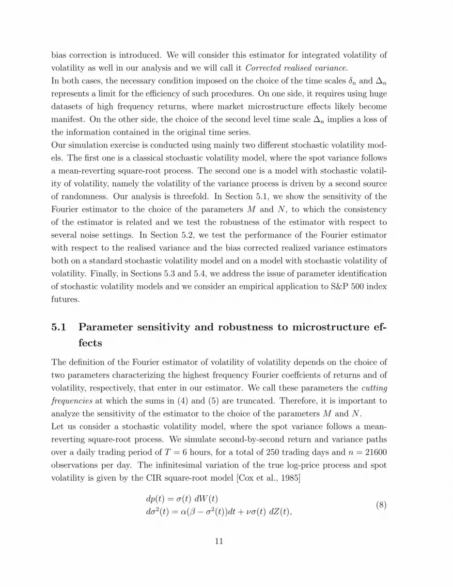
Figure 5: Realised variance: volatility signature plot of the S&P 500 index futures con-
structed over the full sample period. The graph shows average integrated volatility of
volatility constructed for different frequencies measured in minutes (Panel A) and in
number of ticks (Panel B). Note that there are about 8.57 seconds on average between
trades, so that the average annualized 5-minute based realized volatility corresponds to
around the 35th tick.
in the figure, with large variability across the whole dataset. The impact of market mi-
crostructure effects on the five-minute realized volatility measure for the S&P 500 index
futures over the period from 1990 to 2006 can therefore be regarded as negligible. How-
ever, the estimates obtained by calendar time sampling are quite unstable and variable as
the sampling frequency decreases. When sampling in transaction time, the most stable
estimates are obtained for frequencies between 20 and 70 ticks that roughly correspond to
3-10 minutes. In both cases, for low frequencies the realised variance estimator becomes
downwards biased because sparse sampling has a severe impact on the cardinality of the
database. In particular, for any value of n we choose Kn = 2√n. This implies that
most of the data are neglected when estimating the second order quantities so that the
volatility of volatility estimates are poor, especially when we start from sparse sampled
data.
In Figure 6, we plot the volatility signature plot as computed by means of γ2n,N,M using
tick-by-tick data, as a function of the parameter N . The value of the parameter M is set to
3. We can see that for N larger than 150 the estimates become much stable. Taking into
account the mathematical properties of the Fourier estimator, when the trading period
is T = 6.5 hours, a parameter value of say N = 200 corresponds to sampling frequencies
of T/(2N) = 390/400 = 0.9750 min, in the sense that the spectral decomposition in
21

Figure 6: Fourier estimator: volatility signature plot of the S&P 500 index futures con-
structed over the full sample period. The graph shows average integrated volatility of
volatility computed by means of the Fourier estimator, using tick-by-tick data, as a func-
tion of the parameter N . M is set equal to 3.
the frequency space allows to detect phenomena happening at the frequency of about 1
minute, much higher than with the realised variance estimator.
6 Conclusions
We have introduced a new non parametric estimator of the stochastic volatility of volatility
which is particularly suited to work with high frequency data. Our estimator is obtained
in two steps: first we compute the Fourier coefficients of the volatility process using high
frequency observations of the log-returns, then we iterate the procedure with a convolution
of the Fourier coefficients of the volatility process. An advantage of our method lies in the
fact that it does not resort to the estimation of the path of the latent variance of returns,
but it needs only integrated quantities. A theoretical and numerical study of the properties
of our estimator highlights that cutting the highest frequencies in the Fourier expansion
makes this estimator robust to the presence of high-frequency noise components.
In conclusion, our discussion and numerical simulations show that the Fourier estimator of
the volatility of volatility is robust to microstructure effects and efficient in finite sample.
7 Acknowledgements
We wish to thank Frederi Viens and an anonymous referee for their insightful comments
and remarks. We thank the participants in the 5th Annual Modeling High Frequency
Data in Finance conference at Stevens Institute, NJ, USA, in October 2013, for their
interesting and stimulating discussion.
22

References
[Bandi and Russell, 2005] Bandi, F.M. and Russell, J.R. (2005). Microstructure
noise, realized variance and optimal sampling. Working paper, Univ. of Chicago
http://faculty.chicagogsb.edu/federicobandi.
[Barndorff-Nielsen and al., 2008] Barndorff-Nielsen, O.E., Hansen, P.R., Lunde, A. and
Shephard, N. (2008) Designing realized kernels to measure the ex post variation of
equity pricesin the presence of noise. Econometrica, 76 (6), 1481–1536.
[Barndorff-Nielsen and Veraart, 2013] Barndorff-Nielsen, O.E. and Veraart A.E.D. (2013)
Stochastic Volatility of Volatility and Variance Risk Premia. Journal of Financial
Econometrics, 11 (1), 1–46.
[Barucci and Mancino, 2010] Barucci, E. and Mancino, M.E. (2010) Computation of
volatility in stochastic volatility models with high frequency data. International Journal
of theoretical and Applied Finance, 13 (5), 1–21.
[Corsi et al., 2010] Corsi, F., Pirino, D. and Reno, R. (2010) Threshold bipower variation
and the impact of jumps on volatility forecasting. Journal of Econometrics, 159 (2),
276-288.
[Cox et al., 1985] Cox, J.C., Ingersoll, J.E. and Ross, S.A. (1985). A theory of the term
structure of interest rates. Econometrica, 53, 385–408.
[Cuchiero and Teichmann, 2013] Cuchiero, C. and Teichmann, J. (2013) Fourier trans-
form methods for pathwise covariance estimation in the presence of jumps. Working
Paper, arXiv:1301.3602v2.
[Curato and Sanfelici, 2014] Curato, I. and Sanfelici, S. (2014) Fourier estimation of
stochastic leverage using high frequency data, Working paper.
[Hansen and Lunde, 2006] Hansen, P.R. and Lunde, A. (2006) Realized variance and mar-
ket microstructure noise (with discussions). J. Business Econom. Statist., 24, 127–218.
[Heston, 1993] Heston S. (1993) A closed-form solution for options with stochastic volatil-
ity with applications to bond and currency options, Review of Financial Studies, 6:
327–343.
[Hull and White, 1987] Hull, J. and White A. (1987) The pricing of options on assets
with stcohastic volatilities, Journal of Finance, 42: 281–300.
23

[Jacod et al., 2009] Jacod, J., Li. Y., Mykland, P.A., Podolskij, M. and Vetter, M. (2009).
Microstructure noise in the continuous case: the pre-averaging approach. Stochastic
Processes and their Applications, 119, 2249-2276.
[Malliavin and Mancino, 2002] Malliavin, P. and Mancino, M.E. (2002). Fourier series
method for measurement of multivariate volatilities. Finance and Stochastics, 4, 49–61.
[Malliavin and Mancino, 2002a] Malliavin, P. and Mancino, M.E. (2002). Instantaneous
liquidity rate, its econometric measurement by volatility feedback. C.R. Acad. Sci.
Paris, 334, 505–508.
[Malliavin and Mancino, 2009] Malliavin, P. and Mancino, M.E. (2009). A Fourier trans-
form method for nonparametric estimation of multivariate volatility. The Annals of
Statistics, 37 (4), 1983–2010.
[Mancini, 2009] Mancini, C. (2009) Non-parametric threshold estimation for models with
stochastic diffusion coefficient and jumps. Scandinavian Journal of Statistics, 36, 270–
296.
[Mancino and Sanfelici, 2008] Mancino, M.E. and Sanfelici, S. (2008a) Robustness of
Fourier Estimator of Integrated Volatility in the Presence of Microstructure Noise.
Computational Statistics and Data Analysis, 52(6), 2966–2989.
[Mancino and Sanfelici, 2012] Mancino, M.E. and Sanfelici, S. (2012) Estimation of Quar-
ticity with High Frequency Data. Quantitative Finance, 12(4), 607–622.
[Roll, 1984] Roll, R. (1984) A simple measure of the bid-ask spread in an efficient market.
J. Finance, 39, 11271139.
[Stein and Stein, 1991] Stein E., Stein J. (1991) Stock price distributions with stochastic
volatility: analytic approach, Review of Financial Studies, 4: 727-752.
[Vetter, 2011] Vetter, M. (2011) Estimation of integrated volatility of volatility with ap-
plications to goodness-of-fit testing. Working Paper.
8 Appendix: Proofs
Along the proofs, C will denote a constant, not necessarily the same at the different
occurrences.
24

Proof of Theorem 3.2. Under the model assumption (A.I)− (A.II) it is not restrictive
to assume that the volatility process v(t) is a.s. bounded.
We split
γ2n,N,M −
∫ 2π
0
γ2(t)dt
as(2π)2
M + 1
∑|j|≤M
(1− |j|M
)j2 [cj(vn,N)c−j(vn,N)− cj(v)c−j(v)] (11)
+(2π)2
M + 1
∑|j|≤M
(1− |j|M
)j2 cj(v)c−j(v)−∫ 2π
0
γ2(t)dt. (12)
Consider (11). For any |j| ≤M
E[|cj(vn,N)c−j(vn,N)− cj(v)c−j(v)|2]
≤ 2(E[| cj(vn,N)(c−j(vn,N)− c−j(v))|2] + E[|c−j(v)(cj(vn,N)− cj(v))|2]
).
By the definition (4) we write cj(vn,N)− cj(v) as the sum of the following two terms
1
2π
∫ 2π
0
e−ijφn(t)v(t)dt− 1
2π
∫ 2π
0
e−ijtv(t)dt (13)
+1
2π
∫ 2π
0
∫ t
0
e−ijφn(u)DN(φn(t)−φn(u))dp(u)dp(t)+e−ijφn(t)DN(φn(t)−φn(u))dp(u)dp(t),
(14)
where φn(t) = suptk : tk ≤ t and DN(x) is the rescaled Dirichlet kernel defined by
DN(x) = 12N+1
∑|k|≤N e
ikx.
Consider (13)
E[| 1
2π
∫ 2π
0
e−ijt(1− e−ij(φn(t)−t))v(t)dt|2]
≤ (ess sup ‖v‖∞)2 1
2π
∫ 2π
0
|1− e−ij(φn(t)−t)|2dt ≤ (ess sup ‖v‖∞)2j2ρ(n)2.
Consider (14)
E[| 1
2π
∫ 2π
0
∫ t
0
e−ijφn(u)DN(φn(t)− φn(u))dp(u)dp(t)|2]
≤ (ess sup ‖v‖∞)2 1
(2π)2
∫ 2π
0
∫ t
0
D2N(φn(t)− φn(u))dudt ≤ (ess sup ‖v‖∞)2 1
2π
1
2N + 1.
Therefore
E[|cj(vn,N)− cj(v)|2] ≤ 2(ess sup ‖v‖∞)2j2ρ(n)2 +1
π
1
2N + 1.
25

Finally, for any |j| ≤M
E[|c−j(v)(cj(vn,N)− cj(v))|2] ≤ 2(ess sup ‖v‖∞)4M2ρ(n)2 +1
π
1
2N + 1. (15)
Consider now
E[|cj(vn,N)(c−j(vn,N)− c−j(v))|2] (16)
≤ 2(E[|c−j(vn,N)− c−j(v)|4] + E[|cj(v)(c−j(vn,N)− c−j(v))|2]).
The second addend has been estimated in (15). For the first addend consider the de-
composition of c−j(vn,N) − c−j(v) into (13) and (14): then a similar argument using
Burkholder-Davis-Gundy inequality for the estimation of the fourth moment gives
E[|c−j(vn,N)− c−j(v)|4] ≤ C(ess sup ‖v‖∞)4j4ρ(n)4 +1
π
1
2N + 1.
Therefore, for any |j| ≤M
E[|cj(vn,N)(c−j(vn,N)− c−j(v))|2] ≤ C(ess sup ‖v‖∞)4M4ρ(n)4 +M2ρ(n)2 +1
2N + 1.
(17)
By (15) and (17), for any |j| ≤M
E[|cj(vn,N)c−j(vn,N)−cj(v)c−j(v)|2] ≤ C(ess sup ‖v‖∞)4
(M2ρ(n)2 +M4ρ(n)4 +
1
2N + 1
).
Finally, the L2 norm of (11) is less or equal to
CM4 (ess sup ‖v‖∞)4
(M2ρ(n)2 +M4ρ(n)4 +
1
2N + 1
),
which goes to 0 under the hypothesis ρ(n)N → 0 and M4
N→ 0.
Consider (12). Using assumption (A.III), the periodic extension of v(t) to IR with period
2π (which we still denote by v(t)) satisfies v(2π)− v(0) = 0 a.s.. Therefore, applying Ito
formula, we have
(2π)2
M + 1
∑|j|≤M
(1− |j|M
)j2cj(v)c−j(v)−∫ 2π
0
γ2(t)dt = 2
∫ 2π
0
∫ t
0
FM(s− t)dv(s)dv(t),
where FM(x) denotes the rescaled Fejer kernel FM(x) = 1M+1
∑|j|≤M(1− |j|
M)eijx.
Then, we have
E[(
∫ 2π
0
∫ t
0
FM(s− t)dv(s)dv(t))2] = E[
∫ 2π
0
(
∫ t
0
FM(s− t)dv(s))2γ2(t)dt]
≤ E[
∫ 2π
0
γ4(t)dt]12E[
∫ 2π
0
(
∫ t
0
FM(s− t)dv(s))4dt]12 .
26

Applying Burkholder-Davis-Gundy inequality, we get
E[
∫ 2π
0
(
∫ t
0
FM(s− t)dv(s))4dt] ≤ C
∫ 2π
0
∫ t
0
F 4M(s− t)ds dt E[
∫ 2π
0
γ4(s)ds]
≤ C1
M + 1E[
∫ 2π
0
γ4(s)ds].
Finally, the L2 norm of (12) is less or equal to
C1√
M + 1E[
∫ 2π
0
γ4(s)ds].
Proof of Theorem 4.2. For any fixed j, |j| ≤M , we have
E[cj(vn,N)c−j(vn,N)− cj(vn,N)c−j(vn,N)]
= E[2π
2N + 1
∑|h|≤N
ch(εn)cj−h(dpn)2π
2N + 1
∑|l|≤N
cl(εn)c−j−l(dpn)] (18)
+E[2π
2N + 1
∑|h|≤N
ch(εn)cj−h(dpn)2π
2N + 1
∑|l|≤N
cl(dpn)c−j−l(εn)] (19)
+E[2π
2N + 1
∑|h|≤N
ch(εn)cj−h(dpn)2π
2N + 1
∑|l|≤N
cl(εn)c−j−l(εn)] (20)
+E[2π
2N + 1
∑|h|≤N
ch(dpn)cj−h(εn)2π
2N + 1
∑|l|≤N
cl(εn)c−j−l(dpn)] (21)
+E[2π
2N + 1
∑|h|≤N
ch(dpn)cj−h(εn)2π
2N + 1
∑|l|≤N
cl(dpn)c−j−l(εn)] (22)
+E[2π
2N + 1
∑|h|≤N
ch(dpn)cj−h(εn)2π
2N + 1
∑|l|≤N
cl(εn)c−j−l(εn)] (23)
+E[2π
2N + 1
∑|h|≤N
ch(εn)cj−h(εn)2π
2N + 1
∑|l|≤N
cl(εn)c−j−l(dpn)] (24)
+E[2π
2N + 1
∑|h|≤N
ch(εn)cj−h(εn)2π
2N + 1
∑|l|≤N
cl(dpn)c−j−l(εn)] (25)
+E[2π
2N + 1
∑|h|≤N
ch(εn)cj−h(εn)2π
2N + 1
∑|l|≤N
cl(εn)c−j−l(εn)] (26)
The terms (18), (19), (21), (22) are similar. Consider (18): it is equal to
E[1
2π
∑u,u′
DN(tu − tu′)e−ijtu′εuδu′(p)1
2π
∑v,v′
DN(tv − tv′)eijtv′εvδv′(p)].
27

By using the independence between price and noise process, it can be written as
1
2π
∑u,u′
DN(tu − tu′)e−ijtu′1
2π
∑v,v′
DN(tv − tv′)eijtv′E[εuεv]E[δu′(p)δv′(p)]. (27)
Observe that
E[δu′(p)δv′(p)] = 0 if u′ 6= v′
and
E[ε2u] = 2E[η2], E[εuεv] =
−E[η2] if |v − u| = 1
0 if |v − u| > 1.
Therefore (27) is equal to (every term is multiplied by ( 12π
)2)∑u,u′
∑v
DN(tu − tu′)DN(tv − tu′)E[εuεv]E[(δu′(p))2]
= (∑u,u′
D2N(tu − tu′)E[ε2
u] + 2∑u,u′
DN(tu − tu′)DN(tu+1 − tu′)E[εuεu+1])E[(δu′(p))2]
= 2E[η2]∑u,u′
(D2N(tu − tu′)−DN(tu − tu′)DN(tu+1 − tu′))E[(δu′(p))
2].
Using the inequality |DN(tu+1− tu′)−DN(tu− tu′)| ≤ 1−DN(2πn
) and the following limit
in probability
limN→∞
∫ 2π
0
du
∫ 2π
0
DN(u− u′)σ2(u′)du′ = C
∫ 2π
0
σ2(u)du,
we obtain for (27) the asymptotic
2E[η2]E[
∫ 2π
0
σ2(u)du] n(1−DN(2π
n)).
Therefore, the sum over j in the definition of γ2n,M,N gives a term
2E[η2]E[
∫ 2π
0
σ2(u)du]Λ(n,N,M),
where
Λ(n,N,M) =M(M + 1)
3n(1−DN(
2π
n)),
which is O(M2N2
n).
Now compute (20). Note that the terms (23), (24), (25) are similar. For the independence
between noise and price, it is equal to
(2π
2N + 1)2∑|h|≤N
∑|l|≤N
E[ch(εn)cl(εn)c−j−l(εn)]E[cj−h(dpn)] = 0,
28
as E[cj−h(dpn)] = 0 for any j, h and n.
It remains to calculate (26), which is equal to
1
(2π)2
∑v,v′
∑u,u′
e−ij(tv′−tu′ )DN(tv − tv′)DN(tu − tu′)E[εvεv′εuεu′ ]. (28)
We need the fourth moments for the noise process:
E[ε4] = 2E[η4] + 6E[η2]2 (29)
E[ε3uεv] =
−E[η4]− 3E[η2]2 if |u− v| = 1
0 if |u− v| > 1
E[ε2uε
2v] =
E[η4] + 3E[η2]2 if |u− v| = 1
4E[η2]2 if |u− v| > 1
E[ε2uεvεv+1] = −2E[η2]2 if v ≥ u+ 1 or v ≤ u− 2
E[εuε2u+1εu+2] = 2E[η2]2
E[εuεu+1εvεv+1] = E[η2]2 if |u− v| ≥ 2.
In order to compute (28) we proceed as follows (each term has to be multiplied by 1/(2π)2):
I) firstly, we add the terms with coefficient E[η4] + 3E[η2]2∑u
E[ε4u] + 8
∑u
cos(j(tu+1 − tu))DN(tu − tu+1)E[ε3uεu+1]
+6∑u
cos(j(tu+1 − tu))E[ε2uε
2u+1]
= 2(E[η4] + 3E[η2]2) n [(1− cos(j2π
n)) + 4 cos(j
2π
n)(1−DN(
2π
n))].
Therefore, the sum over j in the definition of γ2n,M,N gives
2(E[η4] + 3E[η2]2)1
M + 1
∑|j|≤M
(1− |j|M
)j2 n [(1− cos(j2π
n)) + 4 cos(j
2π
n)(1−DN(
2π
n))]
= 2(E[η4] + 3E[η2]2)Γ(n,N,M),
where Γ(n,N,M) = O(M4
n) +O(M
2N2
n) (we used: cosx = 1− x2
2+O(x4)).
II) Secondly, we add the terms with coefficient 2E[η2]2 and only one summation. We
omit to consider a constant factor c = 30 which multiply each addend, then we have:∑u
cos(j(tu+2 − tu))DN(tu+2 − tu+1)E[ε2uεu+1εu+2]
29

+∑u
cos(j(tu+2 − tu+1))DN(tu+2 − tu+1)DN(tu − tu+1)E[εuε2u+1εu+2]
+∑u
cos(j(tu+2 − tu+1))DN(tu − tu+1)E[εuεu+1ε2u+2]
+2∑u
cos(j(tu+3 − tu+1))DN(tu+3 − tu+2)DN(tu − tu+1)E[εuεu+1εu+2εu+3]
= 2E[η2]2n
− cos(j
4π
n)DN(
2π
n)(1−DN(
2π
n))− cos(j
2π
n)DN(
2π
n)(1−DN(
2π
n))
= 2E[η2]2DN(
2π
n)(1−DN(
2π
n))n
−2(1− 10(j
π
n)2 +O(
j
n)4)
.
Finally, consider the sum over j
2E[η2]2n (1−DN(2π
n))
1
M + 1
∑|j|≤M
(1− |j|M
)j2(1− 10(jπ
n)2 +O(
j
n)4)
= 2E[η2]2Ψ1(n,N,M),
where Ψ1(n,N,M) = O(N2M2
n).
III) Thirdly, we add the terms with coefficient 2E[η2]2 and a double summation. We
omit to write a constant c = 6 which multiplies each term, then we have∑u,v
cos(j(tv − tu))E[ε2uε
2v] + 2 (2
∑u,v
cos(j(tv+1 − tu))DN(tv+1 − tv)E[ε2uεvεv+1])
+4∑u,v
cos(j(tv+1 − tu+1))DN(tu − tu+1)DM(tv − tv+1)E[εuεu+1εvεv+1]
=∑u,v
cos(j(tv − tu))4E[η2]2 + 4∑u,v
cos(j(tv+1 − tu))DN(2π
n)(−2E[η2]2)
+4∑u,v
cos(j(tv+1 − tu+1))D2N(
2π
n)E[η2]2
= 4E[η2]2∑u,v
cos(j(tv − tu))− 2 cos(j(tv+1 − tu))DN(
2π
n) + cos(j(tv+1 − tu+1))D2
N(2π
n)
= 4E[η2]2(1−DN(2π
n))2O(n2).
Then, considering the sum over j, we get a term
2E[η2]2Ψ2(n,N,M),
where Ψ2(n,N,M) = O(M2N4
n2 ). Finally denote Ψ := Ψ1 + Ψ2.
30


