1

AMBIGUITY AVERSION AND ITS EFFECTS ON SAMPLE SELECTION FORLABORATORY ECONOMIC EXPERIMENTS

SUBMITTED BYALEXANDER S. KARLAN ’07

WILLIAMS COLLEGE

ADVISOR: PROFESSOR ROBERT GAZZALE

ABSTRACT:The use of laboratory environments by economists to test and modify theory has steadilyincreased in recent years. Self-selection into the laboratory by subjects is one potentialproblem that may affect the external validity of results found in the laboratory. Walkinginto a laboratory environment, individuals know little information as to what will occur.In this study, I designed an experiment to determine whether ambiguity aversion cancause individuals to not participate in laboratory experiments. I find that more ambiguityaverse individuals are significantly less likely to participate in laboratory sessions whensent a vague solicitation email commonly used by economists. In laboratory settingsdesigned to estimate parameters, this selection has the potential to skew such estimations.My results suggest that economists should take careful consideration as to what mayaffect selection when designing their laboratory experiments.

2

1 INTRODUCTION

Walking into a laboratory environment, individuals usually know little

information as to what will occur. Given this fact, what could play a large role in an

individual’s decision to attend an experiment or not is the ambiguity of the information

presented, which according to Ellsberg (1961) can be considered “a quality depending on

the amount, type, reliability and ‘unanimity’ of information.” Specifically, ambiguity is

the uncertainty about what will actually occur during the experiment created by missing

information. Ellsberg (1961) proposed and demonstrated that when the information given

to an individual was highly ambiguous, the otherwise reasonable individual might not

take actions that conform to the axioms of the subjective expected utility model.

It seems reasonable that some individuals who are more ambiguity averse may

systematically choose not to attend laboratory sessions at all. Furthermore, standard

recruitment emails and other solicitation methods are generally vague as to what tasks

will be performed during the experiment, what the goals of the research are, and how

much money one will actually earn by participating.1 Thus, it also seems reasonable that

individuals who are more averse to ambiguity are less likely to participate in laboratory

experiments when they receive an amorphous invitation to participate. I examine these

important selection effects by testing the following questions: (1) are more ambiguity

averse individuals less likely to participate in experiments in general than less ambiguity

1 In the past, economists have supported their use of vague solicitation mechanisms forthree main reasons: (1) to avoid selection, (2) to avoid having the research agenda affectthe actions of the participants, and (3) to avoid payment expectations affect the actions ofthe participants. However, as this paper demonstrates, vague solicitation mechanisms canactually cause self-selection by inducing more ambiguity averse individuals to notparticipate.

3

averse individuals, (2) are more ambiguity averse individuals less likely to participate in

experiments than less ambiguous averse individuals when the invitation used to solicit

participation is similar to the vague invitations that economists commonly use, and (3)

does self-selection affect outcomes in the laboratory?

The problem of self-selection threatens to completely derail experimentation if it

indeed is a problem that cannot be controlled. While many authors have endeavored to

address the problem of self-selection, few have sought to design an experiment to

determine whether self-selection into the experiment does indeed happen. The

experiment that I ran has two rounds to determine what, if any, effect ambiguity aversion

has on the individuals who choose to participate in experiments. For this study to have

meaning in regards to the use of experiments in economics, I have designed my study to

closely replicate the typical laboratory experimental environment found in economics.

That is, in all phases subjects’ pay was tied to their actions in each session and the

students were selected from the populations that economists generally draw from, both

economics classes and the campus at large. In the first round of the experiment, I

presented modified series of urn questions based on Ellsberg’s canonical urn problem to a

sampling of Williams College students using a protocol that mitigated the issue of self-

selection. Working with Ellsberg’s description of ambiguity averse behavior and the

subjective expected utility model, I categorized individuals in Round 1 into one of three

groups: (1) more ambiguity averse, (2) less ambiguity averse, and (3) individuals who

responses were inconsistent with either theoretical framework2. The individuals in the

third category did not respond in a way that could neither be considered “rational” under

the subjective expected utility model nor ambiguity averse as explained by Ellsberg.

In the second round of the experiment, subjects categorized in Round 1 are sent

2 For a full description of the subjective expected utility model I refer the reader toEllsberg (1961). A concise description of how ambiguity aversion violates the subjectiveexpected utility model is presented later in the paper.

4

one of four invitations varying in detail across two categories: (1) the amount of

information presented in the email regarding how much the subjects are compensated for

attending, and (2) the amount of information presented in the email regarding what tasks

the subjects are asked to perform in the laboratory. Subjects were randomly placed

orthogonally into each of the four email treatments. Who responded to each treatment by

showing up to Round 2 is then observed. As predicted, more ambiguity averse students

are significantly less likely to attend the session when they are sent the baseline

ambiguous email that closely matched standard solicitations where I provide little

information about the tasks attendees will perform and the exact compensation that the

attendees can expect to receive. In terms of mitigating self-selection along preferences for

ambiguity, my results suggest that economists performing laboratory studies should take

careful consideration in drafting solicitation mechanisms. By finding that self-selection

into laboratory settings occurs, this study further emphasizes the need for economists to

be vigilant in considering how self-selection may affect their experiments.

This paper proceeds as follows. Section 2 describes the related research and

motivation to my study. Section 3 presents my experimental design. Section 4 presents

my results. Section 5 concludes.

2 BACKGROUND

Ever since its inception, the scientific method has relied on experimentation as its

cornerstone. One of the very first proponents of the scientific method, Galileo described

the necessity of the experiment in his own words: “in those sciences where mathematical

demonstrations are applied to natural phenomena, as is seen in the case of perspective,

astronomy, mechanics, music, and others, the principles once established by well-chosen

5

experiments, become the foundations of the entire superstructure”(Settle, 1961 p. 19).

Indeed, Feyman (1963) emphasizes this fact when noting that, “the principle of science,

the definition almost, is the following: The test of all knowledge is experiment.

Experiment is the sole judge of scientific ‘truth.’”

As Galileo emphasizes, a critical maintained assumption underlying laboratory

experiments is that the insights gained from such research in the laboratory can be

extended to the real world, a principle come to be known as generalizability or external

validity. The results in the laboratory to date when studying the physical world have

supported this assumption of generalizability. That is, what occurs in the laboratory is

similarly has been found to occur in the natural world, which leads to the fair statement

by Shapeley (1964, p. 43) that “as far as we can tell, the same physical laws prevail

everywhere.”

In their pursuit of universal economic “truths,” economists increasingly use the

traditional experimental model of the physical sciences to understand human behavior.

Holt (2005) documents that experimental economics is a “boom industry,” showing that

publications using the methodology were almost non-existent until the 1960s and have

since grown exponentially, surpassing 50 annually for the first time in 1982, and by 1998

there were more than 200 experimental works published per year.

Yet while experimentation in the laboratory has become increasingly popular

among economists, a number of criticisms have questioned the extent to which laboratory

experimentation produces externally valid results. At the very minimum, for a laboratory

experiment to produce externally valid results the behavior of a sample of subjects who

participate in a particular experiment must be representative of the larger population,

6

whether that larger population be a particular population of interest to the experimenter or

the larger population in general. However, economists cannot force people to participate

in experiments. Individuals decide whether they will participate or not. This decision is

indeed a form of self-selection. The fact that individuals self-select to participate in

experiments leaves open the very real possibility that they self-select systematically,

which creates the possibility that they are unrepresentative of the larger population. This

concern warrants testing to determine whether systematic self-selection into laboratory

experiments does indeed occur.

Since the study of behavioral economics relies to a large degree on laboratory

experimentation, the study of sample selection is of particular importance to this area of

economics. Behavioral economists conduct games in the laboratory to determine if actual

behavior departs from theoretical predictions. However, experimental and behavioral

economics are not necessarily synonymous fields of study. By its very definition,

behavioral economics is the combination of psychology and economics that investigates

what happens in markets in which some of the agents display human limitations and

complications (Mullainathan and Thaler, 2000). In general, behavioral economics refers

to any study which either seeks to relax the assumptions of perfect rationality and

narrowly-defined self interest as defined by classical or neo-classical economists, or tries

to quantify the effects of such a relaxation. While many experimental studies fit in this

framework, some are not entirely behavioral. What makes a study behavioral is a matter

of debate.3

3 Indeed, many economists maintain that all economics is behavioral. However, for mypurposes I maintain the definition of behavioral economics to be the field of study thatseeks to relax the assumptions of perfect rationality and strict self interest, and modelthose relaxations, as defined by standard economic theory.

7

Long before laboratory experimentation was fully embraced, classical economists

traditionally conceptualize the world as being populated calculating, unemotional utility

maximizers dubbed Homo Economicus (Pareto, 1971). As Mullainhathan and Thaler

(2000) point out, the Homo Economicus model has been defended along two main

threads of logic: some claimed that the model was “right” (enough), while most others

argued that it was easier to formalize and practically more relevant to understanding how

most people maximize their utility in markets. Beginning with Allais, the very foundation

of behavioral economics has been anchored in the belief that neither rationale was true.

For example, empirical and experimental evidence has grown against the axioms of

subjective expected utility theory. The controlled environment that the laboratory

provides allows for insights into behavior that field-study could not have easily provided.

It permits economists to answer questions that are hard to attend to in the complex,

perpetually changing real world of the field.

Still, field experiments do contain advantages over laboratory study.4 Field

experiments have many advantages over laboratory experiments in regards to the fact that

field experiments have a certain “realness” that laboratory experiments lack: the stakes in

such experiments more closely emulate real world is just one advantage that is commonly

pointed to when arguing for the benefits of field experimentation. Another advantage is

that participants in field experiments are already self-selected to some extent. Those

individuals who participate in certain markets are not a random sample of the population.

Thus, if one were interested in say the behavior of commodities traders in commodities

markets one would be better studying the traders’ behavior within their market rather

than bring in a random sample of individuals to the laboratory and have the sample play 4 I define a field experiment as an experiment that uses the scientific method to measurethe effects of an intervention in a naturally occurring environment. See Harrison and List(2004) for full taxonomy.

8

games that emulate the commodities market. While the benefits of field experimentation

comes from the “realness” of such an approach, that “realness” also contributes to the

many detrimental aspects of field experimentation. Indeed, the “realness” of field

experimentation can often limit the extensions of the findings. Studying loss aversion in

commodities markets would probably provide little insight into how loss aversion affects,

doctors, teachers, or politicians. In the field, one cannot always control for or necessarily

identify confounding variables that may affect the outcome of such an experiment. In the

laboratory, such effects are more easily identified and controlled.

Experimentation in the laboratory is by definition controlled and artificial which

creates a number of weaknesses for extrapolating real world implications from data

collected by such a method. Critics have called into question whether results found in the

laboratory are applicable to “real people” performing “real tasks” in the “real world”

(Harrison and List, 2004; List and Levitt, 2005). Nevertheless, Smith (1976) views

laboratory experiments as necessary pretests of economic theory and argues that

laboratory experience suggests that all of the characteristics of “real world” behavior that

we consider to be of paramount importance, such as self-interested motivation,

interdependent tastes etc., arise naturally, indeed inevitably in experimental settings.

Smith’s parallelism states that theories ought to hold in environments that do not

explicitly violate the underlying assumptions in the model. Thus, if theoretical

predictions do not hold in the laboratory, than the underlying assumptions of the theory

must need adjusting. Based on this assumption, results from laboratory research on social

preferences have been widely applied outside the laboratory (see Fehr et. al., 1993 and

Camerer, 2003)5.

However, Levitt and List (2005) take issue with this claim and suggest that 5 The definition I use for social preferences here comes from Levitt and List (2005). Theydefine an agent with social preferences as one who has preferences that are measuredover her own and others’ material payoffs. Such preferences might arise due to an agent’spreference for altruism, fairness, reciprocity, or inequality-aversion to name a fewexamples.

9

laboratory studies on social preferences may be a poor guide to behavior outside of the

laboratory due to the fact that within the laboratory environment subject are fully aware

that their behavior is being monitored and thus may be induced to behave in a way that

paints them in a positive light. Indeed, List’s (2005) analysis of the sports card market

revealed that social preferences in the market completely disappeared even though the

agents revealed strong evidence of having social preferences in laboratory environments.

List’s study began with having experienced sports card traders participate in a gift

exchange experiment in the laboratory in which buyers make price offers to sellers for a

baseball card, and in return sellers select the quality level of the good provided by buyers.

In the high scrutiny environment of the laboratory, there was a positive correlation

between the price offer and the card’s quality. However, when the experiment was moved

to the floor of a sports card show, little statistical relationship between price and quality

emerged.6

However, List’s (2003) analysis of the endowment effect in another sports card

market provides strong evidence that the endowment effect found in laboratory studies

persists in markets where agents have experience. Thus, as Smith (1976) prudently

pointed out, laboratory results must be confirmed with field observations to build an

accurate theory of behavior. But in some instances, laboratory results are all that one has

to work with. In particular, in developing parameter estimations for populations, many

economists rely on samples invited to laboratory sessions (Currim and Sarin, 1989;

Currim and Sarin, 1990; Daniels and Keller, 1990; Kahn and Sarin, 1988). For such

laboratory studies, one of the main avenues of criticism attacks the sample from which

the data was collected.

Self-selection into laboratory experiments is one problem that calls into question

6 It should be noted that Benz and Meier (2006) have found a correlation betweenbehavior in laboratory experiments and behavior in the field. In their study, they found acorrelation between how subjects behave in donation experiments in the laboratory andhow subjects behave in naturally occurring charitable giving situations.

10

whether results found in the laboratory can be generalized to the real world (List and

Levitt, 2005).7 That is, human subjects cannot generally be compelled, or forced, to

participate in experiments, but rather, select into them. Individuals observed in

experiments may significantly differ from the population to which the results will be

generalized (List and Levitt, 2005). Orne (1962) found that those who select into

scientific experiments are more likely to be “scientific do-gooders” who are interested in

the study’s goals, while Rosenthal and Rosnow (1969) found that participants are

generally students who readily cooperate with the experimenter and seek social approval.

However, it should be noted that many of these psychological experiments lack

dominance. That is, changes in subjects’ utility in the experiment do not come

predominantly from the reward medium. Thus economists may be concerned about

whether the responses observed in such studies reveal true preferences of the subjects.

Gronou (1974) was one of the first economists to point out that selected samples

are often not representative of the larger general population. Heckman (1979) devised a

generalized econometric method for treating this problem. These criticisms have been

largely addressed by behavioral economists by using Heckman’s method in their data

analysis to create samples which represent the larger population across a number of

demographics but those demographics are often relatively superficial and are based on

variables such as income, race, and geographic location to name a few. While such

7 Levit and List (2005) raise four potential problems in generalizing results of laboratoryeconomic experiments to the real world. First, subjects know that they are being watched.Humans, unlike other lab subjects, know that they are participating in an experiment.Second, the context of an experiment can affect the subject’s behavior and that context isnot completely controlled by the experimenter. Smith (1976), points out, that if suchcontextual considerations are not negligible, the experimenter loses some control over theprocess of induced valuation. Third, laboratory experiments have stakes that are typicallyquite small. Fourth, is the issue of self-selection into lab experiments. Since, my thesisdeals specifically only with the fourth criticism raised by Levit and List, I refer the readerto their paper for a more detailed understanding of the multiple criticisms of labexperimentation.

11

variation in the sample is important, limiting sample selection to cover such variables

may not necessarily create a sample that is representative of the larger population. There

may be key types of people that are consistently left out of certain types of experiments

depending on the method and subject of the experiment.

Nevertheless, the extent to which selection matters depends on the studies goals.

If a study’s goal is to present evidence of an economic anomaly that violates standard

economic theory, the issue of self-selection into the laboratory may not be an issue. For

instance, in demonstrating the existence of the endowment effect in the laboratory, self-

selection is not an important consideration into the validity of such experiments. Since

standard economic theory suggests that any agent’s preference ought not depend on their

endowment, observing the endowment effect in the laboratory effect provides clear

evidence that the assumptions of the theory need adjustment. However, if an economist

wanted to determine “how much” the endowment effect persists in the general population

with a laboratory experiment, selection into the laboratory may be important given that

the endowment effect may persist in some individuals more than others. Selection into

the laboratory may also be important if an economist wanted to investigate how a

particular population, say securities traders, exhibited the endowment effect. In such an

instance, the economist would want to be sure that the individuals who select into the

laboratory are representative of the population of interest.

One common approach to investigating self-selection biases in experiments is to

examine whether professionals, or other representative agents, and students behave

similarly in laboratory experiments (List and Levitt, 2005). For example, Fehr and List

(2004) examine experimentally how Chief Executive Officers (CEOs) in Costa Rica

behave in trust games and compare their behavior with that of Costa Rican students. They

12

find that CEOs are considerably more trusting and exhibit more trustworthiness than

students. These differences in behavior may mean that CEOs are more trusting in

everyday life, or it may be that CEOs are more sensitive to the laboratory’s scrutiny, or

that the stakes are so low for the CEOs that the sacrifice to wealth of making the moral

choice is infinitesimal (List and Levitt, 2005). But this approach does not determine

whether selection bias into the student group occurred, it simply determined that the

student group’s behavior cannot be extended to predict all individuals’ behavior.

Lazaer, Mendelsen, and Weber (2006) suggest that the common selection approach

is too broad to make inferences about market outcomes. They explain that the participants

are locked into the experimental environment and the specific game presented to them

while non-laboratory environments, as in markets, individuals sort based on preferences,

beliefs, and skills. By sorting, they mean the voluntary choice of an activity by an agent.

Those individuals who choose to participate in markets are not a random sample of the

population. Thus, they conclude the ability to sort contaminates inferences from

experimental treatments for the field.

To support their conclusions, Lazaer, Mendelsen and Weber, find that constraining

the test subjects in an experiment has a large effect on the outcomes of the experiment.

Specifically, when individuals are forced to play a dictator game8, 74% of the subjects

share. (Lazaer, Mendelsen, and Weber, 2006). However, when subjects are allowed to

avoid the situation, less than one-third share (Lazaer, Mendelsen, and Weber, 2006). This

reversal of proportions demonstrates that the influence of sorting limits the ability to

generalize experimental findings that do not allow sorting (Lazaer, Mendelsen, and

Weber, 2006).

8 In a dictator game there are two players: (1) the “proposer,” and (2) the “responder.” Inthe game, the proposer’s task is to distribute an endowment between himself and theresponder. The responder then must accept the allocation allotted by the proposer. TheNash equilibrium to this game is for the proposer to keep the entire endowment forthemselves and the responder to receive nothing.

13

One could expand on the findings of Lazaer et al. to postulate that individuals

who participate in laboratory experiments are already sorted. That is, there may be certain

types of people who choose to participate in certain experiments. If this is in fact the case,

knowing who chooses to participate in the experiments may affect the inferences that

economists can make to the larger population from such studies. While it could be of

great value to determine what types of people choose to participate in experiments, there

is little literature on the subject. Specifically, in this study the experiments focused on

how an individual’s averseness to ambiguity may affect their choice to participate in a

given experiment.

Ellsberg initially determined whether an individual was ambiguity averse or not by

asking what has come to be known as his canonical urn problem. In Ellsberg’s original

problem there are two urns, one containing 50 black and 50 red balls (the known urn) and

the other containing 100 balls with an unknown number of those balls being red and

black (the unknown urn). Each urn represents two distinct types of uncertainty. Present in

both urns is the uncertainty as to which outcome will occur: either a red or a black ball

will be drawn. Present only in the unknown urn, however, is ambiguity, the uncertainty

about the probability that each outcome will occur.9 In Ellsberg’s hypothetical

experiments he found that after numerous individuals under non-experimental settings

were offered a prize if they drew a red ball most chose the known urn to draw from; when

he offered a prize to the same individuals again but this time only to those who drew a

black ball most of the same individuals chose the known urn again (Ellsberg, 1961). This

pattern of behavior violates the axioms of subjective expected utility theory and is termed

9 Knight (1921) calls this distinction risk versus uncertainty. In the known urn, Knightwould argue there is risk and in the unknown urn there is uncertainty. Ellberg (1961)distinguishes the two urns by stating that the known urn presents an unambiguousprobability while the unknown urn presents ambiguous probability to the decision maker.

14

ambiguity aversion.10

A “rational” actor conforming to the axioms of subjective utility theory would not

choose the known urn when asked both questions. Rather, they would choose one urn

when betting on drawing the red ball and the other when betting on drawing the black

ball. For instance, if an individual chose the known urn when betting on drawing a red

ball, according to subjective expected utility theory, that same individual should chose

the unknown urn when betting on drawing the black ball. This is because these choices

revealed “believed” probabilities. That is, by choosing the known urn when betting on

drawing a red ball, the individual is revealing she believes that there are more red balls in

the known urn than in the unknown urn. Likewise, if this belief is constant, than she

should also believe that there are more black balls in the unknown urn. By choosing the

unknown urn when betting on pulling a black ball, this individual is acting as if she had a

constant belief about the number of red and black balls in the unknown urn, subjective

utility theory would argue that this individual was unaffected by ambiguity or in other

words, ambiguity neutral. As mentioned in the introduction to this paper, working with

Ellsberg’s description of ambiguity averse behavior and the subjective expected utility

model, I can categorize individuals in Round 1 into one of three groups: (1) more

ambiguity averse, (2) less ambiguity averse, and (3) individuals who responses were

inconsistent with either theoretical framework. The individuals in the third category did

not respond in a way that could neither be considered “rational” under the subjective

expected utility model nor ambiguity averse as explained by Ellsberg.

Numerous researchers, including Slovic and Tversky (1974) and MacCrimmon

10 Subjective expected utility theory was first explicitly described by Savage (1954), butwas inspired by Ramsey (1931). Ramsey combined the von Neumann and Morgenstern(1944) expected utility theory with Finetti’s (1937) calculus of subjective probabilities tocreate what is now known as subjective expected utility theory (Camerer, 1995). For afull list of Savage’s axioms, I refer the reader to Savage’s original paper, SeeFishburn(1988,1989) and Camere and Weber (1992) for technical reviews of subjectiveutility theory.

15

and Larsson (1979), empirically tested Ellsberg’s hypotheses about ambiguity aversion

and found strong support for his hypothetical results. Becker and Brownson (1964) tested

and confirmed two extensions to Ellsberg’s hypotheses: (1) individuals are willing to pay

money to avoid actions involving ambiguity, and (2) some people behave as if they

associate ambiguity with the range of the second-order distributions of the relative

frequency of an event—where the greater the range of the distribution, the greater the

ambiguity implied. Note that ambiguity aversion in economics generally refers to

monetary outcomes. However, since solicitations to participate in economic experiments

in general are ambiguous in regards to both the tasks that will be completed during the

session and the monetary outcomes that can be expected by participating, in Round 2 my

experiment systematically increases information in both dimensions to see if either

affects who shows up to experiments.

3 EXPERIMENTAL DESIGN

This study seeks to determine whether self-selection into laboratory experiments

occurs through a very simple experimental design. In the first round of the experiment, I

collected a sampling of Williams College students in a manner that mitigated the self-

selection issue. Those with consistent responses I classified as either more ambiguity

averse or less ambiguity averse, while those with inconsistent responses were not

classified but nevertheless left in the sample. All the subjects participating in Round 1

were then randomly assigned a treatment email solicitation so that each treatment sample

was balanced according to the original distribution observed in Round 1. To solicit

participation in Round 2, I sent out four treatment emails with each subject receiving one

email. The emails varied in the amount of detail provided in regards to what tasks would

be performed in the session and the compensation that the subjects could expect to

16

receive by participating. I then recorded who responded to each treatment by showing up

to the Round 2 sessions .

3.1 ROUND 1 DESIGN: MEASURING BASELINE AMBIGUITY AVERSION

In Round 1, I determine the ambiguity preferences of a sample of Williams

College students so that it can be determined if ambiguity aversion causes students to

self-select into certain experiments. Normally, economists rely on either passive

solicitation mechanisms, active solicitation mechanisms, or a database of previous

participants. Common passive solicitation mechanisms are posters posted around campus,

sign-up sheets, or other means of announcements requiring individuals who wish to

participate to actively contact the experimenter. An active solicitation mechanism would

be when an economist actively approaches a potential subject, usually students in their

economics classes. Both active and passive solicitation mechanisms can cause most non-

field economic experiments to be conducted using students who self-select into

experiments.

The typical solicitation for participation in an economic experiment by means of a

mass email could not be utilized in Round 1 for that would give the students an

opportunity to self-select into the sample. In creating this sample, the selection issue had

to be systematically controlled. I developed a protocol so that self-selection by the

students is minimized.

The protocol is simple. I solicited to participate in a manner so that their

opportunity costs were low and the potential payoffs to participating were high. The first

environment in which they were approached to participate was at then end of an

introductory economics class. Cooperating professors allocated ten minutes at the end of

their class for a single session. The students are randomly selected as to the extent they

17

chose to take an introductory economics course, which most students at Williams College

do, and they happened to be in an introductory economics taught by a cooperating

professor11. Since in past research, economics professors have solicited participants for

their experiments from their classes, the classroom seemed like the logical place to begin

to build a sample of participants.12 94 subjects in the Round 1 sample were recruited in

first-year economics classes.

At the beginning of each session, the instructions and the potential rewards to

participating were explained and then the students were given the opportunity not to

participate and leave the class. The students were then asked to fill out a handout (see

Appendix A) with 10 of Ellsberg’s hypothetical canonical urn gambles and provide some

personal information. Five urn distributions are presented in the Round 1 handout

beginning with 50 red balls and 50 black balls in the known urn and ending 10 red balls

and 90 black balls in the known urn. Remember, at each urn distribution a subject is

presented with two gambles: (1) if I were to give you $10 if you pulled a red ball on your

first try from which urn would you pick and (2) if I were to give you $10 if you pulled a

red ball on your first try from which urn would you pick? Thus, ten gambles are

presented to the subject in Round 1. In each gamble the student will have to indicate

which urn they would draw from.

The in-class sessions were supplemented by soliciting participation from students

in the two major libraries on campus, Schow and Sawyer. A given area in the library was

11 I would like to specially thank Professor Gazzale and Professor Love for generouslyoffering their class time to further my research.12 Bull, Schotter, and Weigelt (1987), Ariely, Lowenstein and Prelec (2003), andKahneman, Knetsch and Thaler (1990) are just a few of the many researchers who haveused economics students in their research.

18

chosen for a session, and everyone in sight was approached and asked to complete the

survey. The students were randomly selected from the campus community in so far as

they happened to be in that given area during a given session. After the students were

approached, the potential subjects were given the opportunity to not participate. As in the

in-class sessions, none of the participants were told that they would be potentially

contacted in the future. 103 subjects in the Round 1 sample were recruited in the library.

Out of the 203 individuals approached both in class and in the libraries, only two

declined to participate. None of the students in the classroom sessions decided to opt out

of participating while two students approached in the library decided not to participate.

This indicates that once the students were already in close proximity to the experimenter,

either the opportunity cost of participating was relatively low when compared to the

potential benefits of participating in the experiment or the cost of not participating was

relatively high.

At the end of all the sessions 1 out of 3 of the students were selected to potentially

receive a payment. Then one of their urn answers was randomly selected to be used to

determine their payment. If they selected the unknown urn, then a computer randomly

chose the urn’s distribution. If they draw the proper ball, determined again by a

computer, according to that particular question then they will receive the payment of that

hypothetical gamble.

Based on responses to the questionnaire, individuals participating in the first

phase were then classified as either more ambiguity averse (MAA) or less ambiguity

averse (LAA). To determine this, the responses were sorted according to when they

began to deviate from general ambiguity averse behavior, as originally explained by

19

Ellsberg, to behavior consistent with the axioms of subjective utility theory. That is, the

responses were sorted on the basis of when the subjects began to stop choosing the

known urn when betting on pulling both a red and black ball. At any given known

distribution, students who chose the known urn when betting on pulling both a red and

black ball can be said to be ambiguity averse at that particular distribution according to

Ellsberg. Subjects whose behavior could not be determined by some already established

behavioral or theoretical framework, as explained earlier, were categorized as neither

MAA nor LAA but were still left in the sample.

3.2 ROUND 2 DESIGN

Round 2 is designed to determine (1) whether the degree to which a subject is

ambiguity averse effects their participation in laboratory experiments and (2) if there is a

difference in the outcomes of that experiment that is due to a difference in group

composition. To achieve this, the experimental design of Round 2 has to closely simulate

a typical economic laboratory experiment, from the solicitation of students to the

laboratory session itself.

The first question of interest, whether certain types of students are more likely to

participate in experiment, will be observed through the group composition of those

persons who choose to participate in a particular session. The four treatment emails used

are detailed in the table below:

20

Students from the original sample collected in Round 1 were randomly assigned one of

four solicitation mechanisms explained in the above table. Email (1) is an ambiguous

email that is based on the standard solicitation used by the economics department at

Williams College that was ambiguous in terms of what tasks were to be performed in the

session and what the subjects could expect to receive in compensation. Email (2) is an

email that is detailed in terms of what tasks were to be performed in the session but

ambiguous with terms of what the subjects could expect to receive in compensation.

Email (3) is an email that is ambiguous in terms of what tasks were to be performed in

the session but was detailed in terms of what the subjects could expect to receive in

compensation. Email(4) is an email that is detailed in terms of both what tasks were to be

performed in the session and what the subjects could expect to receive in compensation

(see Appendix C for emails). The emails that contain the same amount of detail

regarding either the tasks to be performed or the payment to be expected contained the

exact same wording. For example, Email (1) contained the same wording in regards to

what tasks were to be performed as Email (3).

In the emails that were ambiguous in regards to what tasks were to be performed,

I provided no information as to what was to occur during the session. In the emails that

Ambiguous Detailed

Ambiguous Ambiguous Task, Ambigous Payment (1)

Detailed Task, Ambigous Payment (2)

Detailed Ambiguous Task, Detailed Payment (3)

Detailed Task, Detailed Payment (4)

Table 1

Detail Regarding The Tasks:

Detaild Regading the Payment:

Treatment Emails

21

were detailed in regards what tasks were to be performed, I told recipients that the

experiment consisted of two sections. In the first section of the experiment, I told

recipients that they would have the opportunity, in private, to donate part of their show up

fee to a charity and that the amount they gave would be matched by the experimenter. In

the second section, I told the recipients they would be asked to make a series of decisions.

For each decision, they would be asked to choose one of two options where the outcome

of each option is uncertain. In some decisions, they would know the probability of each

outcome within each option. In other decisions, they would not know the probability of

each outcome for one of the options. In the email, I told the recipients that after they

made their decisions, I would randomly select some of their decisions and they will be

paid according to their choices. In the emails that were ambiguous in regards to the

payment, I informed the recipients that by participating in the experiment they would

earn either $10 or $20 and that the session would last about 30 minutes. In the emails that

were detailed in regard to the payment, I informed the recipients that by participating in

the experiment they would have a 50% chance of earning $10 and a 50% chance of

earning $20 and that the session would last about 30 minutes.

After being categorized as either MAA or LAA in Round 1, the subjects were

randomly assigned so that the ambiguity categories would be orthogonal to the email

treatments. That is, the same proportional number of MAA subjects, LAA subjects, and

subjects with inconsistent responses were randomly placed in each treatment. All emails

were sent out using ExLab13 software, a standard software used for emailing mass

solicitations in economic experiments.

13 http://exlab.bus.ucf.edu/

22

The instrument used in the sessions during Round 2 was designed to approach the

second questions on a variety of levels (see Appendix D for instrument). Included in the

instrument were a series of four tasks: a public good dictator game, a series of ordered

lottery gambles, a replication of the Round 1 instrument, and finally an optimism survey.

The public goods dictator game and the replication of the Round 1 instrument differ in

the degree to which ambiguity theory allows for strong predictions to be made as to how

MAA and LAA play may differ while the ordered lottery gambles and the survey on

optimism were included to determine whether ambiguity aversion is correlated with

either risk aversion or optimism.

Task 1: Public Good Dictator Game

The first task presented in the instrument was a form of the public-good dictator

game. The student was given the opportunity to donate as much or as little of their $10

show up fee to two charities, one known and one ambiguous, and was notified that any

donation will be matched by the experimenter. To control for nuisance variables, four

versions of the public-good game were created, while each subject participating in Round

2 was randomly assigned a public-good game so that the ambiguity classifications were

orthogonal to each game.

The two charities chosen for this experiment were Oxfam and Habitat for

Humanity, two charities that were viewed as being close analogues operating in slightly

different settings. In each instrument, one was randomly assigned as the ambiguous

charity and was described in such a manner. When detailed information was provided

about Oxfam in the instrument, I described Oxfam as a nonprofit organization that works

to minimize poverty through relief and development work in Africa. I described Habitat

23

for Humanity as a nonprofit organization that builds homes for those in need that has

been instrumental in Hurricane Katrina relief efforts in the United States. When Oxfam

was described ambiguously, I described it as a nonprofit organization that works to

alleviate poverty in Africa. Similarly, when Habitat for Humanity was described

ambiguously, I described it as a nonprofit organization that works to help victims of

natural disasters in the United States. The order in which the known and ambiguous

charities are presented in the instrument was also randomized so that any supremacy

effect of one charity being viewed before the other can be controlled. Thus, subjects who

returned to Round 2 were presented with one of four possible instruments. The

instrument received was randomized according to the subjects’ previous classification in

Round 1.

In designing this first task in the Round 2 instrument, non-anonymity effects were

controlled for. In the past, lack of anonymity has been found to contribute to pro-social

behavior by subjects. Hoffman et al. (1994), for example, find that 22 of 48 dictators

(46%) donate at least $3 of a $10 pie under normal experimental conditions, but when

subject-experimenter anonymity is added, only 12 of 77 dictators (16%) give at least $3.

Based on their observations, Hoffman et al. (1994, p. 371) concludes that observed

“behavior may be due not to a taste for “fairness” (other-regarding preferences), but

rather to a social concern for what others may think, and for being held in high regard by

others.” This experiment mitigated the non-anonymity effects by giving the subjects four

envelopes to give the illusion of anonymity.14 I discreetly numbered each envelope on the

inside with an identification number that correlates to the paper instrument that the

subjects were given. The four envelopes were (1) an envelope labeled “start” containing 14 There was no deception in this experiment. While anonymity was an illusion, it was notexplicitly guaranteed, and thus I do not know what inferences the subjects may havedrawn.

24

the subjects initial endowment of 10 $1 bills, (2) an envelope labeled “me” which

subjects will move money into to keep for them selves, (3) an envelope labeled “1”

corresponding to the first charity presented in the instrument, and (4) an envelope labeled

“2” corresponding to the second charity presented in the instrument. In this task, subjects

moved $10 from the “start” envelope to the other envelopes as they saw fit.

Task 2: Holt-Laury Lottery Gambles

The second task presented in the instrument was included to further assess what

the ambiguity aversion instrument from Round 1 was really measuring. Some students

categorized as LAA may simply be more comfortable with estimating probabilities than

the students categorized as MAA. A series of ordered gambles based on the gambles first

developed by Holt and Laury (2002) and later modified by Jamison, Karlan, and

Schechter (2006) were presented to the subjects as the second task. The series of gambles

included ten binary choices between two lotteries. The exact payoffs to each gamble are

shown in Appendix D part III. The first choice was between a “safe” lottery that paid

$5.50 with a 10% chance and $4.40 with a 90% chance (Option A in the instrument) and

a “risky” lottery that paid $10.60 with a 10% chance and $.28 with a 90% chance (Option

B in the instrument). In the first choice, the first lottery was both risk-dominant and had a

higher expected value. The probability of the higher payoff in each lottery increased by

10% as the choices progressed until the final choice was between $5.50 with certainty

and $10.60 with certainty, so that the second lottery dominated in all respects (Jamison

et. al, 2006). As the probability of the high outcome increases, a person should cross over

to Option B (Holt and Laury, 2002). The number of choices that a subject chooses Option

A before they choose Option B determines their tolerance for risk (Holt and Laury,

2002). That is, the longer a subject chooses Option A, the more risk averse they are.

25

Task 3: Modified Ellsberg Urn Gambles

The third task included in the instrument was a replication of the Round 1

instrument. The replication of this game provides a clear line of inquiry to determine if

self-selection into laboratory experiments can affect laboratory outcomes. If I were to

have simply run Round 1 in the laboratory, self-selection could possibly skew the

observed distribution. If the distribution of responses in Round 1 differs from the

distribution of responses in Round 2, then I will be able to determine whether this

difference is due to any difference in group composition. Furthermore, such a replication

allows me to determine if subjects are consistently ambiguity averse over time and

whether the degree to which they are ambiguity averse changes. Some inconsistency is

expected, due to the fact that individuals have experience with the instrument and more

importantly were not paid in between Round 1 and Round 2. Thus, they may experience

unnecessary regret due to possible belief that they were one of the individuals randomly

selected but did not win. However, this is probably unlikely given that in Round 1 they

were notified that only one in three individuals would be selected, Furthermore, if there is

variation in responses between Round 1 and Round 2, given that the instrument provides

an ordered scale with which I can measure ambiguity aversion, I can look to see if the

responses are correlated. If the responses remain correlated, then I can infer to a certain

degree how Round 1 participants who did not return to Round 2 would have responded

had they participated in Round 2.

Task 4: Optimism Survey

The fourth task was included to again further assess what the ambiguity aversion

instrument from Round 1 was measuring. To determine whether MAA students are

26

simply less optimistic than LAA students and thus more averse to unknown

circumstances, included in the instrument was a series of questions originally designed by

Scheier, Carver, and Bridges (1994) to measure an individual’s optimism. Ten questions

were asked, three were positively worded, three were negatively worded, and four are

filler controls. For each question the student either chooses A, I agree a lot, B, I agree a

little, C, I neither agree nor disagree, D, I disagree a little, and E, I disagree a lot. An A

response is graded as one point, B is graded as two points, C is graded as three points, D

is graded as four points, and E is graded as five. The most pessimistic total score is 14

while the most optimistic score is 22 (see Appendix D part IV).

The students were compensated based on their responses to the first three sections

of the instrument. Each subject who participated in Round 2 was given a $10 show up fee

and told that they would be compensated for the other tasks presented in the experiment,

though the exact amount they would receive depended on their choices, and on random

chance. After the first task, the subjects kept the whatever was remaining of their $10

show up fee. Even though between the second and third task in the instrument subjects

would make 20 decisions, they were notified that only one of these would end up being

used to determine their payment. For each subject, an urn question was randomly selected

for payment. The Round 2 experiment was designed so that the subjects would on

average earn between $10 and $20 for a 30-minute session. The average payment for

Round 2 was $10.19.

To avoid scheduling conflicts, three Round 2 sessions were held. Each treatment

was randomly divided equally into two groups. The first group for each treatment was

invited to attend the first session on Tuesday February 20th, 2007 and the second group

27

for each treatment was invited to attend the second session on Tuesday February 27th,

2007. Finally, to further control for scheduling conflicts, all the subjects who did not

attend the first two sessions were sent the same treatment email inviting them to attend

the third session on Wednesday March 7th 2007.

3.3 ROUND 2 HYPOTHESES

The treatments considered in this experiment differ in the method in which I

solicit experimental subjects’ participation. While there are several models that depart

from the neo-classical subjective expected utility model which can model decisions under

ambiguity, those models are limited in so far as they predict decisions based on unknown

lotteries (Kahn and Sarin, 1988). Moreover, they do not differentiate between more or

less ambiguity averse individuals (Kahn and Sarin, 1988). Nevertheless, ambiguity theory

allows for limited predictions as to who would respond more to the various treatment

emails. Working from Becker and Brownson’s (1964) first extension of Ellsberg’s

hypotheses that individuals are willing to pay money to avoid actions involving

ambiguity, I develop four hypotheses.

Ceteris paribus, MAA subjects can be expected to be more likely to pay money to

avoid actions involving ambiguity than LAA subjects since they are more ambiguity

averse. This proposition leads to the first hypothesis:

Hypothesis 1: Less ambiguity averse students are more likely to participate in

economic experiments than more ambiguity averse students. 15

15 The null hypothesis for Hypothesis 1 is that there will be no difference in participationbetween less ambiguity averse students and more ambiguity averse students.

28

Despite the fact that the more detailed emails provided a great deal of information, the

information is by no way complete and guaranteed with certainty. Thus, even when sent

the more detailed emails, MAA would be more willing to forgo a payment opportunity by

not showing up to session to avoid the ambiguous scenario of walking into the laboratory.

The second hypothesis follows from the same proposition as the first:

Hypothesis 2: LAA subjects will respond at a higher rate than MAA subjects to

the baseline ambiguous email providing ambiguous information in regards to the

task that would be completed in the session and the payment that the participants

could expect to receive by participating.16

Since the baseline email provides little information in either dimension, MAA subjects

would be more willing to forgo a payment opportunity that LAA students by not

participating in Round 2. This was the second hypothesis tested.

The third hypothesis tested was the softest hypothesis regarding how subjects

would respond to the treatments:

Hypothesis 3: MAA subjects would respond at a different rate to the emails that

were detailed in terms of what the subjects could expect to receive in

compensation than to the baseline ambiguous email. 17

I cannot make any strong predictions as whether MAA will respond at higher or lower

rates to the detailed payment email than the baseline ambiguous email because I do not

know for certain how MAA individuals read the information provided in regards to the

16 The null hypothesis for Hypothesis 2 is that there will be no difference in the responserate of LAA and MAA subjects who were sent the baseline ambiguous email.17 The null hypothesis for Hypothesis 3 is that they will be no difference in the responserate of MAA students who were sent emails that were detailed in regards to payment andMAA students who were sent the baseline ambiguous email.

29

payment. MAA individuals may read the ambiguous payment information as a “certain

payment” and regard the more detailed information about payment as having a higher

variance. If this is the case, then working with Becker and Brownson’s (1964) second

extension of Ellsberg’s hypothesis, the MAA students would be more likely to respond to

the emails that provide ambiguous payment information.

Since ambiguity aversion theory does not address how ambiguity averse

individuals treat non-monetary information, there can be no strong predictions made

about how response rates will differ between the emails that contain more detailed

information about the tasks the subjects will complete in the laboratory and the emails

that contain more detailed information about the compensation the subjects can expect to

receive by attending the session. Specifically, I cannot make any predictions based on

ambiguity aversion theory as whether the response rate of MAA subjects will differ

between the detailed task, ambiguous payment treatment email than to the baseline

ambiguous email. Still, it seams reasonable to expect that MAA subjects would respond

at higher rates to the email solicitations that provide more detailed information about the

tasks to be performed during the session.

Some predictions can be made as to how MAA and LAA play during the public

goods game may differ based loosely on ambiguity theory, which leads to my fourth

hypothesis:

Hypothesis 4: At the very least, MAA and LAA are expected to give differently

to the unknown charity due to the lack of information provided about the charity.

However, there is no literature that relates ambiguity aversion to charitable giving that

allows for strong hypotheses.

30

If the student responses remain consistent from Round 1 to Round 2, there are

clear predictions that can be made about group composition affect the results of the

Round 1 game that is replicated in the instrument of Round 2. If more LAA students

attend sessions, then the average responses to the canonical urn questions will be skewed

towards LAA behavior. Any change in the group composition from Round 1 to Round 2

should have some effect on the average responses. This effect could lead us to conclude

that self-selection into the laboratory environment could skew the results of the

laboratory study if that study was designed to estimate population parameters.

4 RESULTS

4.1 ROUND 1 RESULTS: MEASURING AMBIGUITY AVERSION

Students had the opportunity to deviate from ambiguity averse behavior at five known

urn distributions. The further along in the series they deviated, the more ambiguity averse

the subject is determined to be. Beginning with the 50 red balls, 50 black balls, the

known distribution urns are numbered from 1 to 5. As the known urn number increased

by one, the number of red balls in the known urn decreased by 10 and the number of

black balls in the known urn increased by 10. Thus, known urn number 5 contained 10

red balls, 90 black balls. For each subject in Round 1, I recorded the numbered urn at

which they deviated from ambiguity aversion along with their demographic data. If a

particular never deviated from ambiguity averse behavior, I recorded 6 for that subject.

This methodology orders ambiguity aversion from 1, ambiguity neutral, to 6, very

ambiguity averse. Using that scale, I then ranked the subjects according to their

ambiguity aversion. Below are two figures. The first figure compares the probability

31

distribution of Round 1 responses with Round 2. The second compares the cumulative

distribution of Round 1 responses with Round 2.

The number of red balls in the known urn can be calculated as follows: # of Red Balls = 50 - (Decision # - 1) * 10

The number of red balls in the known urn can be calculated as follows: # of Red Balls = 50 - (Decision # - 1) * 10

Figure 1Probability Distribution Of Urn Choices Where Subjects Deviated From Ambiguity

Averse Behavior

0

0.1

0.2

0.3

0.4

0.5

0.6

0.7

0.8

1 2 3 4 5 6

Urn Number

Prop

ortio

n

Round 1 Round 2

Figure 2Cumulative Distribution of Urn Choices Where Subjects Deviated From Ambiguity Averse Behavior

0

0.2

0.4

0.6

0.8

1

1.2

1 2 3 4 5 6

Urn Number

Prop

ortio

n

Round 1 Round 2

32

Note the large proportion of students in Round 1 who deviated from ambiguity averse

behavior when reaching the second known urn with 40 red balls and 60 black balls.

Taking this large proportion into account, I created a rule that classified subjects as either

MAA or LAA. LAA students were classified as those students who deviated from

ambiguity averse behavior when arriving at the second known urn in the series

(henceforth, Decision # 2), with the distribution of 40 red balls, 60 black balls. MAA

students were classified as those subjects who deviated from ambiguity averse when

arriving at the third urn in the series (henceforth, Decision # 3) with a distribution of 30

red balls, 70 black balls, or later. Thus, subjects who deviated from ambiguity averse

behavior when arriving at the fourth known urn in the series (henceforth, Decision # 4),

fifth known urn in the series (henceforth, Decision #5) or subject who never deviated

(henceforth, Decision # 6) were classified as MAA.

After the students were classified, I excluded six from the Round 1 sample either

because they were Economics Thesis students who found out about the study’s goals or

because they were not on campus when Round 2 was to be conducted. Of the 197

students in the Round 1 sample, I classified 115 classified as LAA and 54 as MAA.

Table 3 provides the full distribution of Round 1 data (See Appendix B for Data).

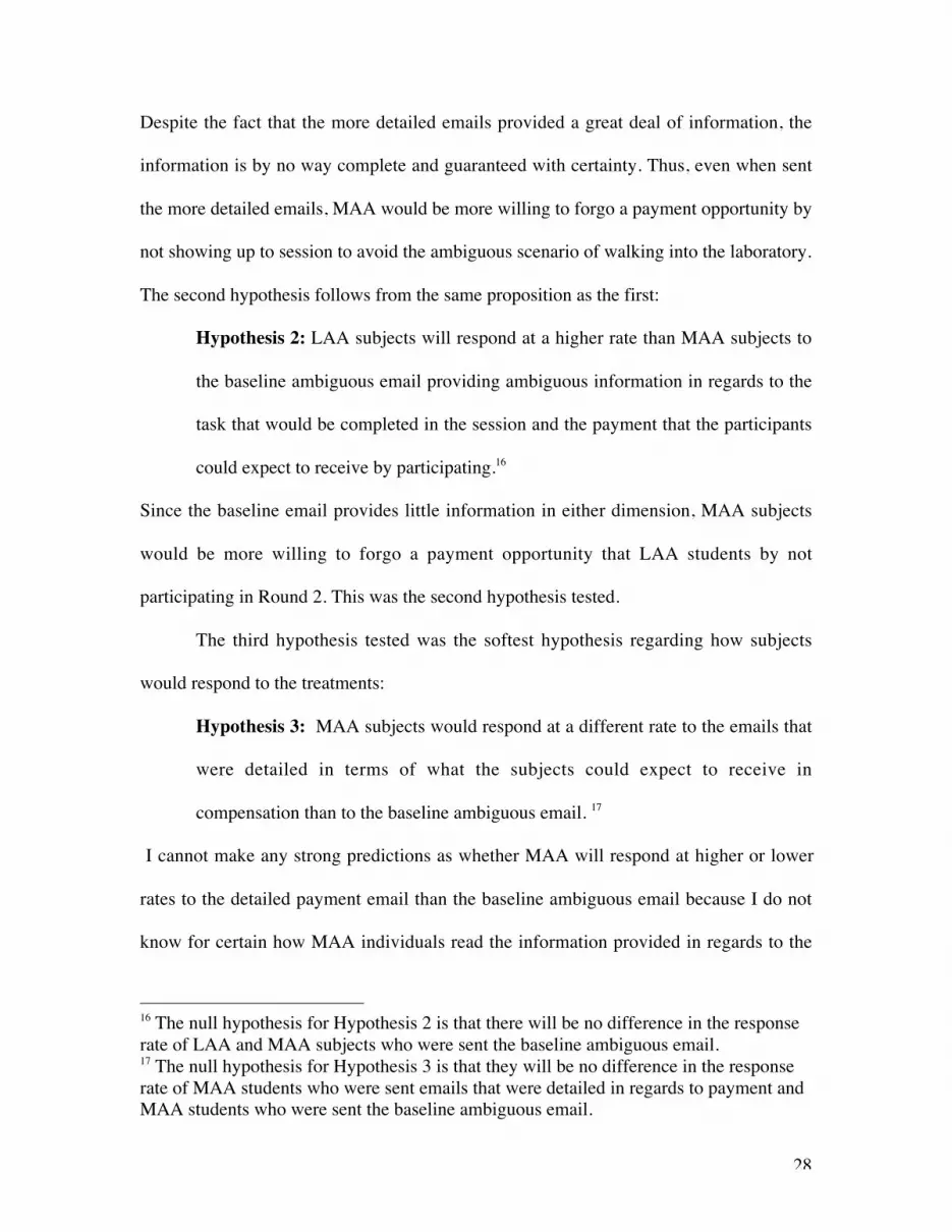
4.2 DETERMINANTS OF ROUND 1 AMBIGUITY AVERSION CLASSIFICATION

During Round 1 I collected demographic data from each subject. To determine if

ambiguity classification in Round 1 is determined by any demographic information, a

series of probit models is estimated below. Marginal effects are reported for coefficients

so that holding all else equal, one can determine the increased probability that a subject

33

would participate given the stated determinants. All independent variables in the model

are binary indicator variables.

As shown in Table 2, none of the demographic data predicts who was classified as either

MAA or LAA. This lends evidence that my ambiguity aversion classifications are

uncorrelated with any observable characteristics of the subjects, other than how they

responded on the Round 1 instrument. Since subjects with inconsistent responses in

Round 1 are a small proportion of my data set and because they are excluded from much

of my data analysis, a probit regression was not estimated for those subjects.

4.3 BALANCE OF TREATMENTS IN ROUND 2

Binary Dependent Variable:More Ambiguity Averse in

Round 1(1)

Female 0.029(.072)

Round 1 Conducted in Library 0.119(.103)

Round 1 Conducted in Gazzale's Class 0.076(.167)

Freshman -0.077(.132)

Sophomore

Junior -0.087(.103)

Senior -0.167(.092)

Economics Major 0.043(.118)

Psychology Major -0.093(.211)

R^2 0.018

Table 2Determinants Of Ambiguity Classification

Probit

Marginal effects are reported for coefficients. Robust standard errors are inparenthesis. * indicates significance at 10 percent. ** at 5 percent. *** at 1percent. In column one, the dependant variable equals zero if the subjectdid not show up to round 2 and one if the subject did show up. Variablesare ommited due to collinearity. Only information from Juniors and Seniorswas included in the major data since Williams students do not declare theirmajor until the end of their Sophmore year. A probit regression thatpredicts being classified as Less Ambiguity Averse in Round 1 has the exactsame coefficients for all variables but of the opposite sign.

34

Before looking to see if ambiguity aversion plays a role in self-selection into

laboratory settings, I first show that my Round 1 sample was properly balanced across

treatments. To be clear, I only attempted to balance the created ambiguity classifications

across the four treatments. No attempts were made to balance any other metrics. Below is

a table that investigates how well I balanced my treatments:

Remember, I classified the subjects into one of three groups, MAA, LAA, and

inconsistent responders based on their responses in Round 1. Looking at Table 2 we see

that there is no significant difference between any of the treatments. Given the very high

p-values for the F-test comparing the four treatments (greater than .98), I can be confident

that the proportion of MAA, LAA, and inconsistent responders were properly balanced

across the four treatments in this dimension.

However, the proportion of females and subjects who participated in Round 1 in

the library does not appear to be balanced across treatment groups as well. Since the

Treatment:

Received Ambiguous Solicitation

Email

Received More

Detailed Solicitation

Emailst-stat:

(2)<>(3)

Received Ambiguous Solicitation

Email

Received Detailed Task and Ambigous Payment

Received Ambiguous Task and Detailed Payment

Received Detailed Task and Detailed Payment Prob > F

(1) (2) (3) (4) (5) (6) (7) (8)

More Ambiguity Adverse in Round 1 0.265 0.277 0.187 0.265 0.28 0.28 0.271 0.998(.063) (.04) (.446) (.454) (.468) (.449)

Less Ambiguity Adverse in Round 2 0.633 0.615 -0.1877 0.633 0.6 0.62 0.625 0.989(.07) (.04) (.467) (.495) (.49) (.489)

Inconsistent Responses in Round 1 0.102 0.108 0.1187 0.102 0.12 0.1 0.104 0.988(.044) (.026) (.306) (.328) (.303) (.309)

Female 0.388 0.5 1.364 0.388 0.5 0.42 0.583 0.2165(.070) (.041) (.492) (.505) (.499) (.498)

Round 1 Conducted in Library 0.489 0.534 0.532 0.5 0.64 0.44 0.52 0.2297(.072) (.041) (.51) (.48) (.501) (.504)

Round 1 Conducted in Gazzale's Class 0.347 0.264 -1.12 0.303 0.179 0.285 0.232 0.381(.069) (.036) (.464) (.386) (.456) (.426)

Number of Observations 49 148 49 50 40 48

In columns 1 and 2 standard errors are in parentheseses. * significant at 10%; ** significant at 5%; *** significant at 1%. A subject is Less Ambiguity Averse if theybegan choosing the unknown urn when betting on the red ball when the known distribution was 40 red, 60 black. A subject is More Ambiguity Averse if they beganchoosing the unknown urn when betting on the red ball when the known distribution was 30 red, 70 black or higher. Column 3 presents the t-statistic for the twosample t-test for the data in column 1 and column 2. Column 8 provides the p-value for the F-test comparing columns 4, 5, 6, and 7.

Treatment Means & Standard Deviations

Table 3Balance of Treatments

35

means in Table 1 correspond to proportions, the proportion of females in the baseline

ambiguous email treatment is lower than in the more detailed email treatments (.38

versus .5). Also, the proportion of students that participated in Round 1 in the library

varies across treatments, though the variation is not statistically significant. Similarly,

while the proportion of students who participated in Round 1 in Professor Gazzale’s

classroom differs across treatments, the variation is not statistically significant. Still,

because of these differences, I will control for observable demographics in my core

analysis.

4.1 EFFECT OF AMBIGUITY AVERSION ON SELECTION INTO ROUND 2

The next step in my analysis involves looking at looking at the effect of ambiguity

aversion on return rates. Of the 197 subjects Round 1 participations, 36 (18.3%)

responded for Round 2.

36

Below, Table 4 shows that the same proportion of MAA and LAA subjects

participated in Round 2:

Earlier, Figure 1 shows non-parametrically that the distribution of ambiguity aversion

appears the same in Round 1 as it does in Round 2. Furthermore, in the table above, a two

sample t-test shows no significant difference between the proportion of MAA and LAA

students who returned to Round 2. Given these results, I cannot reject the null hypothesis

that more ambiguity averse individuals participate in laboratory experiments at the same

rate as less ambiguity averse individuals.

Sample Frame: AllMore Ambiguity Averse

in Round 1Less Ambiguity Averse

in Round 1

Inconsistent Responses in

Round 1t-stat:

(2)<>(3)(1) (2) (3) (4) (5)

Panel A: Full sampleProportion Returned for Round 2 0.183 0.185 0.189 0.052

(0.027) (0.053) (0.036)Proportion More Ambiguity Averse in Round 2 0.485 0.600 0.435 -0.856

(0.083) (0.163) (0.106)Panel B: Received Ambiguous Solicitation Email

Proportion Returned for Round 2 0.341 0.154 0.419 1.7131*(0.072) (0.104) (0.090)

Proportion More Ambiguity Averse in Round 2 0.467 1.000 0.385 -1.6653(0.133) (0.000) (0.140)

Panel C: Received More Detailed Solicitation EmailsProportion Returned for Round 2 0.1389 0.195 0.118 -1.206

(.029) (.0626) (.032)Proportion More Ambiguity Averse in Round 2 0.55 0.5 0.5833 0.3493

(.114) (.1889) (.1486)Panel D: Demographics and Sample Size Data

Number of observations in full study 197 54 122 21

Number of participants who returned in Round 2 36 10 23 3

Female 93 28 56 9

Freshman 74 21 50 3

Sophomore 55 18 31 6

Junior 37 10 21 6

Senior 29 5 19 5

Economics Major 22 7 13 2

Psychology Major 4 1 3 0

Round 1 Conducted in Class 94 24 64 6

Round 1 Conducted in Library 103 30 58 15

Means & Standard Errors

Table 4

Standard errors are in parentheses. * significant at 10%; ** significant at 5%; *** significant at 1%. A subject is Less Ambiguity Averse if they began choosingthe unknown urn when betting on the red ball when the known distribution was 40 red, 60 black. A subject is More Ambiguity Averse if they began choosingthe unknown urn when betting on the red ball when the known distribution was 30 red, 70 black or higher. Subjects with inconsistent responses wereexcluded in the two-sided t tests.

Summary Statistics

37

However, LAA students were significantly more likely to participate in Round 1

when sent the baseline ambiguous email than MAA subjects. Of the subjects sent the

baseline ambiguous email, 41.9% of LAA subjects participated in Round 2 while only

15.4% of the MAA chose to participate. After performing both a two-sample t-test and its

non-parametric alternative, the Wilcoxon rank-sum test, this difference was found to be

significant at the 10% level (p-values for both tests equal .09). On the other hand, when

subjects were sent the more detailed emails, the proportion of MAA and LAA subjects

who participated did not differ significantly. These two observations taken together lend

evidence to the conclusion that if a laboratory experiment’s email solicitation is vaguely

written, the vague solicitation can lead to a biased sample of individuals participating in

the experiment.

Table 5 below further separates the email treatments to determine the type of

ambiguity subjects are responding to in the email: ambiguity regarding what tasks will be

performed or ambiguity regarding the expected payment.

38

Of the four treatment emails, only the baseline ambiguous email and the detailed task,

ambiguous payment email elicited statistically different participation from MAA and

LAA subjects. Interestingly, LAA subjects participated at the lowest rate when receiving

the detailed task, ambiguous payment email. It appears that increasing the detail about the

tasks to be performed in the email solicitation drives down the participation by LAA

subjects. However, after further investigation of the determinants of who participates, this

effect was found to be negligible.

To further investigate the determinants of who participates in Round 2, a series of

probit models estimated from the data are presented in Table 6.18 Marginal effects are

18 Due to the lack of good data, information on majors and other demographic variableswere not included in these regressions.

Sample Frame: AllMore Ambiguity Averse

in Round 1Less Ambiguity Averse

in Round 1 t-stat: (2)<>(3)(1) (2) (3) (5)

Panel A: Full sampleProportion Returned for Round 2 0.183 0.185 0.189 0.052

(0.027) (0.053) (0.036)Proportion More Ambiguity Averse in Round 2 0.485 0.600 0.435 -0.856

(0.083) (0.163) (0.106)Panel B: Baseline Ambiguous Solicitation

Proportion Returned for Round 2 0.341 0.154 0.419 1.713*(0.072) (0.104) (0.090)

Proportion More Ambiguity Averse in Round 2 0.467 1.000 0.385 -1.6650(0.133) (0.000) (0.140)

Panel C: Detailed Task & Ambigous Payment Solicitation Proportion Returned for Round 2 0.136 0.357 0.033 -3.171***

(.052) (.133) (0.033)Proportion More Ambiguity Averse in Round 2 0.667 0.60 1.00

(0) (.2449) (0)Panel D: Ambiguous Task & Detailed Payment Solicitation

Proportion Returned for Round 2 0.133 0.071 0.161 0.809(.051) (.0714) (.067)

Proportion More Ambiguity Averse in Round 2 0.500 1.000 0.600(.245)

Panel E: Detailed Task & Detailed Payment Solicitation EmailProportion Returned for Round 2 0.140 0.154 0.133 -0.174

(.053) (.104) (.063)Proportion More Ambiguity Averse in Round 2 0.333 0.500 0.250 -0.516

(.210) (.25) (0.25)

Table 5

Means & Standard Errors

Standard errors are in parentheses. * significant at 10%; ** significant at 5%; *** significant at 1%. A subject is Less Ambiguity Averse if they beganchoosing the unknown urn when betting on the red ball when the known distribution was 40 red, 60 black. A subject is More Ambiguity Averse if theybegan choosing the unknown urn when betting on the red ball when the known distribution was 30 red, 70 black or higher. Subjects with inconsistentresponses were excluded in the two-sided t tests. Of the 36 subjects who returned in Round 2, 10 were categorized as More Ambiguity Averse, 23 werecategorized as Less Ambiguity Adverse, and 3 had inconsistent responses in Round 1. In Panel C and D, t-tests on Proportion More Ambiguity Averse inRound 2 could not be performed due to the fact that one variable was perfectly predictive. Nevertheless, the mean and standard errors were left in to givea sense of how individuals who recieved those two emails "switched" their responses.

Email Treatments

39

reported for coefficients so that holding all else equal, one can determine the increased

probability that a subject would participate given the stated determinants. All independent

variables in the model are binary indicator variables.

Table 6 shows a number of interesting findings. First, students that participated in

Round 1 in first year economics classes are significantly more likely to participate in

Round 2. This finding is not surprising. Economics students already exhibit an interest in

the discipline by taking courses in the major. Furthermore, the email solicitations were

sent from Professor Robert Gazzale’s email account to mitigate any subject’s ability to

link Round 1 with the Round 2 solicitations. Since more than half of the students

approached in first year economics students were Professor Gazzale’s students, this effect

could be an artifact of Rosenthal and Rosnow (1969) findings that participants are

generally students who readily cooperate with the experimenter and seek social approval.

Or first year economics students may simply want to get in the good graces of a professor

Binary Dependent Variable:Participated

Round 2Participated

Round 2Participated

Round 2Paricpated Round 2

Participated Round 2

Paricpated Round 2

(1) (2) (3) (4) (5) (6)

More Ambiguity Averse in Round 1 0.0123 0.016 0.074 0.074(.064) (.063) (.133) (.133)

Less Ambiguity Averse in Round 1 -0.074 -0.075(.133) (.133)

Email with Ambiguous Task and Ambiguous Payout 0.1636* 0.251** -0.063 0.25 -0.062(.10) (.122) (.120) (.122) (.120)

Email with Ambiguous Task and Detailed Payout -0.118 -0.134 -0.117 -0.134(.081) (.106) (.082) (.106)

Email with Detailed Task and Ambiguous Payout 0.001 0.117 0.001 0.115(.091) (.115) (.0915) (.159)

Email with Ambiguous Task and Ambiguous Payout AND More Ambiguity Averse in Round 1 -0.15* -0.15*(.046) (.046)

Email with Ambiguous Task and Detailed Payout AND More Ambiguity Averse in Round 1 -0.115 -0.115(.082) (.082)

Email with Detailed Task and Ambiguous Payout AND More Ambiguity Averse in Round 1 0.347 0.342(.291) (.294)

Email with Ambiguous Task and Ambiguous Payout AND Less Ambiguity Averse in Round 1 0.37* .37*(.261) (.262)

Email with Ambiguous Task and Detailed Payout AND Less Ambiguity Averse in Round 1 0.201 0.202(.263) (.263)

Email with Detailed Task and Ambiguous Payout AND Less Ambiguity Averse in Round 1 -0.164 -0.163(.055) (.074)

Female -0.066 -0.05 -0.049 -0.049 -0.049 -0.049(.057) (.058) (.056) (.056) (.056) (.056)

Round 1 Conducted in Library -0.187*** -0.183*** -0.171*** -0.171*** -.164** -.164**(.057) (.058) (.057) (.057) (.073) (.073)

Round 1 Conducted in Gazzale's Class 0.009 0.009(.073) (.073)

R^2 0.074 0.116 0.181 0.181 0.181 0.181Marginal effects are reported for coefficients. Robust standard errors are in parenthesis. * indicates significance at 10 percent. ** at 5 percent. *** at 1 percent. In column one, the dependantvariable equals zero if the subject did not show up to round 2 and one if the subject did show up. The individuals who responded inconsistently in round 1 and therefore could not be classified asmore or less ambiguity averse were excluded from this regression. Variables in column 3 are ommited due to collinearity.

ProbitDeterminants Of Whether A Subject Shows Up To Round 2

Table 6

40

in the department. While Professor Gazzale was no longer the students’ professor when

Round 2 was performed, I performed Wilcoxon rank-sum test confirming Gazzale’s

students showed up more than others (p-value= .0004)19. However, when an indicator

variable for Gazzale’s students was added to my probit models, the coefficient was

statistically insignificant (p-value= .90 for both models). Furthermore, when Wilcoxon

rank-sum tests were performed to see if Gazzale’s students who participated in Round 2

differed in their Round 1 ambiguity classification from other subjects who participated

after being sent each treatment, no significant difference was found.20

Notice that students who received the baseline ambiguous email are more likely

to participate in Round 2. This finding may encourage economists to continue to use

ambiguous emails to simply keep their participation rate high. However, when a subject

is sent the base line fully ambiguous email and they are more ambiguity averse, they are

19 A Wilcoxon ran sum test is used here to avoid distributional assumptions regarding adata. The test is appropriate because even though it is testing a binary variable, the binaryvariable can still be ranked in a meaningful manner. Furthermore, there is no cause forconcern that the binary variable is tied in this test. Still, a t-test confirms the difference(p-value=.0003).20 When comparing the Round 1 ambiguity classification of students who participated inRound 2 after receiving the fully ambiguous email, no significant difference was foundbetween students who were recruited in Round 1 in Gazzale’s class and others whenperforming a Wilcoxon rank sum test (p-value = .765). Similarly, using a Wilcoxon ranksum test no significant differences were found for the detailed task, ambiguous pay emailtreatment, ambiguous task, detail pay email treatment, and detailed task, detailed payemail treatment (p-values =.1573, .3173, .4795 respectively). Furthermore, whencomparing the Round 1 ambiguity classification of students who participated in Round 2after receiving the fully ambiguous email, no significant difference was found betweenstudents who were recruited in Gazzale’s class and other first year economics studentswhen performing a Wilcoxon rank sum test (p-value=.583). Similarly, using a Wilcoxonrank sum test no significant differences were found for the ambiguous task, detail payemail treatment and the detailed task, detailed pay email treatment (p-values= .2207and.4795 respectively). However, of the first year economics students sent the detailedtask, ambiguous email treatment in Round 2, only Gazzale’s students participated.

41

significantly less likely to participate. The significance of this interaction term in columns

four and six clearly confirms my second hypothesis.

Table 6 does not confirm the previous observation that increasing the detail about

the tasks to be performed in the email solicitation drives down the participation by less

ambiguous averse subjects. When an individual is LAA and receives the detailed task and

ambiguous payment email solicitation they are less likely to participate, but the

coefficient is insignificant (p-value = .17). However, when a subject is sent the base line

fully ambiguous email and they are less ambiguity averse, they are significantly more

likely to participate. The significance of this interaction term in columns four and six

further confirms my second hypothesis.

4.3 INCONSISTENT RESULTS BETWEEN ROUND 1 AND ROUND 2

In Round 2 I expected the subjects responses to be consistent with their Round 1

responses. However, in Round 2 there was a slightly different payment scheme. Tables 4

and 5 indicate that there was a large degree of “switching” between MAA and LAA

behavior from Round 1 to Round 2. That is, subjects who were classified in Round 1 as

MAA exhibited in behavior in Round 2 that classified them as LAA. Note that in Table 2

Panel A, the proportion of subjects categorized in Round 2 as MAA does not

significantly differ between subjects who were categorized in Round 1 as MAA or LAA.

Indeed, a 43.5 % of the subjects categorized in Round 1 as LAA who participated in

Round 2 exhibited MAA behavior when completing the exact same series of modified

Ellsberg urn problems. In all of my results that I have presented so far, I assumed that my

classifications in Round 1 are meaningful. I made this assumption because this switching

42

is an artifact of the very strict artificial rule that I developed to separate the Round 1

distribution into two clear groups. A more specific measure of ambiguity averseness

would be to look at the decision number where the subjects started exhibiting behavior

consistent with the axioms of subjective utility theory. The higher the decision number,

the more ambiguity averse they are. Using this metric, I looked to see there was a

correlation in responses between Round 1 and Round 2. Using a Pearson pairwise

correlation, I found a positive correlation coefficient of .4461 between the Round 1 and

Round 2 responses, significant at the 1 percent level (See Figure 3 below for scatter

plot)21.

Figure 3

This positive correlation between the decision number where the subject deviated from

ambiguity averse behavior in Round 1 and the decision number where the subject

deviated from ambiguity in Round 2 explains why there would be many subjects

21 The scatter plot above displays jittered data points.

43

reclassified under my strict rule. While the Round 1 responses may not be a perfect

measure of ambiguity aversion, the fact that the Round 1 and Round 2 responses are

correlated allows me to safely assume that the Round 1 responses were indeed measuring

ambiguity aversion.22

To investigate whether there were any determinants of which subjects exhibited

inconsistent responses, I estimated a series of probit models below:

As shown in the above table, I found no significant determinants for inconsistent

responses between Round 1 and Round 2. This leads me to conclude that such behavior is

idiosyncratic and random.

22 This analysis is on only 36 observations and is thus low powered. A significantcorrelation with a small sample size provides solid evidence that the correlation is indeedreal.

Inconsistent Between Round 1 and Round 2

(1)-0.011(.05)0.067(.06)

-0.061(.069)-0.013(.045)0.05

Marginal effects are reported for coefficients. Robust standard errors are inparenthesis. * indicates significance at 10 percent. ** at 5 percent. *** at 1percent.The individuals who responded inconsistently in round 1 andtherefore could not be classified as more or less ambiguity adverse wereexcluded from this regression. Since a binary indicatator variable for MoreAmbiguity Averse in Round 1 was used, a coeffificient for Less AmbiguityAverse in Round 1 would be of the same magnitude as the coefficient ofMore Ambiguity Averse in Round 1 but of the opposite sign.

Round 1 Conducted in Gazzale's Class

Female

R^2

More Ambiguity Averse in Round 1

Round 1 Conducted in Library

Table 7

Determinants of Inconsistent Responses Between Round 1 and Round 2Probit

Binary Dependant Variable:

44

4.4 CORRELATION BETWEEN AMBIGUITY AVERSION, RISK AND OPTIMISM

To be sure that my instrument is not measuring something other than ambiguity

aversion, I checked to see if either risk aversion or optimism were correlated with

ambiguity aversion. Remember, the Holt-Laury lottery involves a series of choices

between a safe (Option A) and risky (Option B). As one moves along the series, the risky

option becomes more appealing. A rational decision maker would only switch between

the choices at one and only one point. Thus, the further along in the series a subject

switches from the safe option to the risky option, the more risk averse that particular

subject is. By recording at which lottery decision the subjects switch, the Holt-Laury

lotteries provide a means to rank subjects according to their risk aversion. The Spearman

rank correlation between observed ambiguity aversion and risk aversion in Round 2

yields an insignificant p-value of .59. Furthermore, a Pearson correlation yields a

negative correlation coefficient of –.2012 that is insignificant with a p-value of .26. While

these findings suggest that the subjects tolerance for ambiguity is uncorrelated with their

tolerance for risk, they are based on only 36 observations and are thus low powered.

Nevertheless, the lack of correlation also leads me to suspect that LAA subjects in Round

2 were not simply more comfortable with probabilities than MAA students.

The optimism survey conducted in Round 2 also provided a metric with which to

rank subjects. The higher the subjects score on the survey, the more optimistic they are. A

Pearson correlation between observed ambiguity aversion and optimism in Round 2

yields an insignificant correlation of .0063 with a p-value of .9711, leading me to believe

45

that LAA students are not merely more optimistic about unknown outcomes than MAA

students.23

4.3 EFFECTS OF SELF-SELECTION ON LABORATORY OUTCOMES

The Round 2 results demonstrate that in the baseline ambiguous email treatment,

MAA subjects are less likely to participate. This self-selection means little if it does not

alter laboratory outcomes. I consider two scenarios. First, a researcher might not be

explicitly interested in ambiguity aversion in their laboratory research but ambiguity

aversion might plausibly affect subjects’ behavior. I determine how selection into the

laboratory based on ambiguity aversion may affect lab outcomes in this scenario by

looking at the responses in the public good dictator game. Second, a researcher may want

to develop parameter estimations for ambiguity aversion using laboratory sessions. By

looking at the Round 2 responses to the Ellsberg urn gambles (the replication of the

Round 1 instrument) I determine how selection may affect such parameter estimations

4.3.1 PUBLIC GOOD DICTATOR GAME

The public-good dictator game provided a possible environment in which MAA

and LAA play may differ in Round 2. However, despite the fact that non-anonymity

effects were controlled, the high rate of giving observed by both MAA and LAA subjects

yielded no observable differences between MAA and LAA play. Of the 36 subjects

participating in Round 2, 30 subjects gave to at least one of the charities while 15

23 As stated earlier, this analysis was based on 36 observations and thus is a low poweredtest. A significant correlation may be found with a larger sample.

46

subjects gave equally to both charities. Table 8 below provides summary statistics for

giving behavior in the public good dictator.

The two-sample t-tests presented in Table 8 confirm that there is no significant difference

in giving behavior between by either MAA or LAA subjects. Furthermore, Wilcoxon

rank-sum tests of the amount given to both known and unknown charities confirm that

there is no significant difference in giving by subjects classified in Round 1 as either

MAA or LAA subjects (p-values: .93 and .33, respectively). Similarly, Wilcoxon rank-

sum tests of the amount given to both known and unknown charities confirm that there is

no significant difference in giving by subjects classified in Round 2 as either MAA or

LAA subjects (p-values: .32 and .60, respectively). To further see if subjects classified as

MAA in either Round 1 or Round 2 gave differently than LAA subjects, in Table 9 I

report the results of a series of probit models:

Sample Frame: All

More Ambiguity Averse in Round 1

Less Ambiguity Averse in Round 1

t-stat: (2)<>(3)

More Ambiguity Averse in Round 2

Less Ambiguity Averse in Round 2

t-stat: (5)<>(6)

(1) (2) (3) (4) (5) (6) (7)Subjects Gave To At Least One Charity 0.848 0.900 0.826 -0.530 0.938 0.765 -1.382

(0.063) (0.100) (0.081) (.063) (.106)Subjects Gave Equally To Both Charities 0.545 0.500 0.565 0.336 0.563 0.529 -0.185

(.088) (.167) (.106) (.128) (.125)Subjects GaveTo Known Charity 0.758 0.800 0.739 -0.364 0.875 0.647 -1.540

(.076) (.133) (.094) (.085) (.119)Subjects Gave To Unknown Charity 0.727 0.900 0.652 -1.473 0.813 0.647 -1.052

(.079) (.100) (.102) (.101) (.119)Amount Subjects Gave in $ To Known Charity 2.606 2.700 2.565 -0.175 3 2.24 -1.102

(.348) (.716) (.402) (.508) (.474)Amount Subjcects Gave in $ To Unkown Charity 2.510 3.300 2.174 -1.294 2.500 2.530 0.036

(.404) (.895) (.425) (.483) (.654)

Table 8Giving Summary StatisticsMeans & Standard Errors

Standard errors are in parentheses. * significant at 10%; ** significant at 5%; *** significant at 1%. A subject is LessAmbiguity Averse if they began choosing the unknown urn when betting on the red ball when the known distributionwas 40 red, 60 black. A subject is More Ambiguity Averse if they began choosing the unknown urn when betting on thered ball when the known distribution was 30 red, 70 black or higher. Subjects with inconsistent responses wereexcluded in the two-sided t tests.

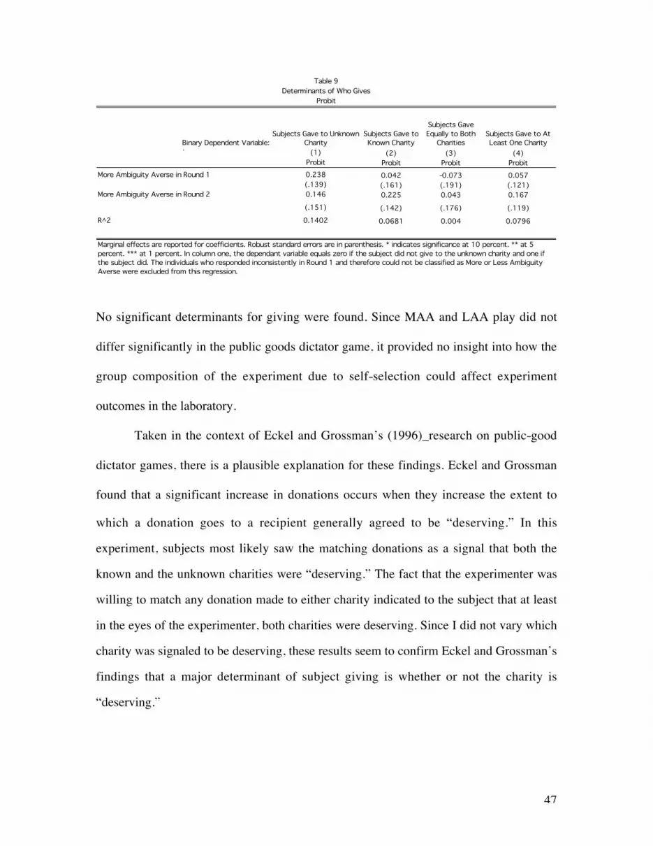
47

No significant determinants for giving were found. Since MAA and LAA play did not

differ significantly in the public goods dictator game, it provided no insight into how the

group composition of the experiment due to self-selection could affect experiment

outcomes in the laboratory.

Taken in the context of Eckel and Grossman’s (1996)_research on public-good

dictator games, there is a plausible explanation for these findings. Eckel and Grossman

found that a significant increase in donations occurs when they increase the extent to

which a donation goes to a recipient generally agreed to be “deserving.” In this

experiment, subjects most likely saw the matching donations as a signal that both the

known and the unknown charities were “deserving.” The fact that the experimenter was

willing to match any donation made to either charity indicated to the subject that at least

in the eyes of the experimenter, both charities were deserving. Since I did not vary which

charity was signaled to be deserving, these results seem to confirm Eckel and Grossman’s

findings that a major determinant of subject giving is whether or not the charity is

“deserving.”

Subjects Gave to Known Charity

Subjects Gave Equally to Both

CharitiesSubjects Gave to At Least One Charity

(2) (3) (4)Probit Probit Probit

0.042 -0.073 0.057(.161) (.191) (.121)0.225 0.043 0.167

(.142) (.176) (.119)

0.0681 0.004 0.0796

More Ambiguity Averse in Round 2 0.146

(1)

0.238More Ambiguity Averse in Round 1

Probit

(.139)

(.151)

Subjects Gave to Unknown CharityBinary Dependent Variable:

Table 9Determinants of Who Gives

Probit

`

0.1402

Marginal effects are reported for coefficients. Robust standard errors are in parenthesis. * indicates significance at 10 percent. ** at 5 percent. *** at 1 percent. In column one, the dependant variable equals zero if the subject did not give to the unknown charity and one if the subject did. The individuals who responded inconsistently in Round 1 and therefore could not be classified as More or Less Ambiguity Averse were excluded from this regression.

R^2

48

4.3.2 REPLICATION OF ROUND 1 INSTRUMENT

While I found no difference in giving behavior, the replication of Round 1

instrument provided a clear mode of analysis to determine if self-selection into laboratory

experiments can affect laboratory outcomes. Specifically, the replication of the Round 1

instrument will allow me to determine whether parameter estimations of ambiguity

aversion would have been skewed by selection into the laboratory. Since some

economists use laboratory sessions to estimate parameters, this study provides evidence

against the reasonableness of such a practice. If I wanted to estimate parameters for

ambiguity aversion, I would have followed Kahn and Sarin’s (1988) procedure by asking

each subject to indicate the known probability of winning that would make him/her

indifferent between the known urn and the ambiguous urn.24 Still, for the sake of

conducting comparative static analysis, my questions provide sufficient cross-sectional

variation to conduct the analysis at hand.

Simply comparing responses in Round 1 to Round 2 is not appropriate because

three treatment emails provided more information than standard solicitation mechanisms

24 Kahn and Sarin (1988) ask their subjects the following:

There are two urns containing red and black balls. A ball will be chosen randomlyfrom one of the urns; if the ball is red, you will win $100. Urn 1 has an unknownproportion of red and black balls totaling 200. How many red balls (total of redand black balls equals 200) would you put in Urn 2 to make you indifferentbetween the two urns?

Instead of replicating Kahn and Sarin’s (1988) procedure, I decided to expand Ellsberg’s(1961) original urn problem to a series of ordered urn questions for a number of reasons.With Kahn and Sarin’s method provide a more continuous measure, it requires morecomplicated analytical reasoning and thus provides the opportunity for subjects tomiscalculate and reveal a distribution that in fact they are not indifferent between the twourns. My method is far simpler. However, since my distributions change by 10, there isno exact point at which I can determine indifference. For instance, a subject who deviatesfrom ambiguity averse behavior when the know urn had a distribution of 40 red, 60 blackcould be indifferent between the known urn and the unknown urn at any distribution from49 red, 51 black to 40 red, 60 black.

49

for economic laboratory experiments. To determine whether self-selection could produce

non-representative outcomes in the laboratory, I first look to see if the sample of students

who participated in Round 2 after receiving the baseline ambiguous email differed from

those who did not. Because all four treatments were not perfectly balanced across all

demographics, I then investigate how Round 2 responses would differ from Round 1 if

everyone in Round 1 were to have received the baseline ambiguous solicitation email.

Unfortunately, switching introduces uncertainty as to which response for those who

participated in Round 2 represent true preferences. Therefore, I perform both analyses

two different ways, First, I assume that the preferences revealed in Round 1 are true

preferences. Second, I assume that the preferences in Round 2 are true preferences.

When comparing the urn number where subjects deviated from ambiguity averse

behavior, I found a significant difference using a Wilcoxon rank-sum test between those

who participated between the subjects who participated in Round 2 and those who did not

when assuming that Round 1 behavior revealed true preferences for those who attended

Round 2 (p-value: .08). However, when assuming that Round 2 behavior revealed the

true preferences of the subjects that participated in that round, using a Wilcoxon rank

sum tests I found no significant difference in the urn number where subjects deviated

from ambiguous behavior between the subjects who participated in Round 2 and those

who did not (p-value: .51). This insignificant difference is due to inconsistent responses

between Round 1 and Round 2 of those who participated after receiving the baseline

ambiguous email solicitation.

However, this analysis is flawed because it looks only at the subjects who

received the baseline ambiguous email. The fact that my treatments were not balanced

50

perfectly across all demographics creates room for error. I perform two hypothetical

analyses to answer the question, if everyone in Round 1 received the fully ambiguous

email, would the distribution of responses to the modified series of Ellsberg urn questions

in Round 2 significantly differed from Round 1. In both analyses I make the following

assumption:

Assumption 1: Subjects who deviated from ambiguity averse behavior at the

same Urn number would respond at the exact same rate to the baseline ambiguous

email.

The practical meaning of this assumption is explained explicitly in the context of subjects

who deviated from ambiguity averse behavior at Urn # 2 as follows. I assumed that

subjects who deviated from ambiguity averse behavior at Urn # 2 and were not sent the

fully ambiguous email, would respond at the exact same rate as those who deviated at the

same decision number and were sent the fully ambiguous email. Out of the 31 subjects

who deviated from ambiguity averse behavior at Urn # 2 and were sent the fully

ambiguous email, 13 returned. Thus, of the subjects who deviated from ambiguous averse

behavior at Urn # 2 and were not sent the fully ambiguous email, I assumed that 42%

would have returned to Round 2 had they been sent the fully ambiguous email. Given this

assumption, I created a hypothetical dataset based on the observed response rates to the

baseline ambiguous email in Round 2. For my first hypothetical analysis I made an

additional assumption:

Assumption 2: Responses between Round 1 and Round 2 will remain consistent.

51

While this assumption runs contradictory to my observations in Round 2, I use it as a

basis for my hypothetical analysis to determine how a hypothetical Round 2 data set

might differ if all of the subjects in Round 1 were sent the baseline ambiguous email. A

two-sample Wilcoxon rank-sum test comparing the hypothetical Round 2 distribution to

the observed Round 1 distribution yields a p-value of .01, leading me to conclude that the

two distributions are significantly different. In figures 4 and 5, I present the differences in

both probability and cumulative distributions.

The number of red balls in the known urn can be calculated as follows: # of Red Balls = 50 - (Decision # -1) * 10. “Hypothetical Round 2 Without Switching” refers to the distribution I created for my firsthypothetical analysis while “Hypothetical Round 2 With Switching” refers to the distribution I created formy second hypothetical analysis.

Figure 4Comparison of the Probability Distribution Of Round 1

0

0.1

0.2

0.3

0.4

0.5

0.6

0.7

0.8

0.9

1

1 2 3 4 5 6

Urn Number

Perc

ent

Round 1 Hypothetical Round 2 Without Switching Hypothetical Round 2 With Switching

52

The number of red balls in the known urn can be calculated as follows: # of Red Balls = 50 - (Decision # -1) * 10. “Hypothetical Round 2 Without Switching” refers to the distribution I created for my firsthypothetical analysis while “Hypothetical Round 2 With Switching” refers to the distribution I created formy second hypothetical analysis.

In performing my second hypothetical analysis, I modify assumption 2 to account

for the changes in responses observed with-in subjects between Round 1 and Round 2. To

create a more realistic hypothetical distribution for Round 2, I assume the following:

Assumption 3: Subjects who were not previously sent the fully ambiguous email

in Round 2 will respond consistently with like subjects who attended Round 2.

Assumption 3 simply means that I assume that individuals who did not show up to Round

2 but deviated from ambiguity averse behavior at that same decision number in Round 1

as subjects who did participate, would deviate from their Round 1 responses in a similar

Figure 5Comparison of the Cumulative Distribution of Round 2

0

0.2

0.4

0.6

0.8

1

1.2

1 2 3 4 5 6

Urn Number

Perc

ent

Round 1 Hypothetical Round 2 Without Switching Hypothetical Round 2 With Switching

53

manner. The assumption becomes more clear as I explain how I formulated the rules for

my second hypothetical analysis.

Using assumption 3, I was able to formulate a series of simple rules as to how the

hypothetical subjects attending Round 2 would change their responses from Round 1 to

Round 2. To formulate the rules, I categorized the subjects who attended Round 2

according to their Round 1 responses and then looked to see the number of subjects in

each category deviated and what response they deviated to. For instance, in Round 2, 23

subjects attended who original deviated from ambiguity averse behavior at Urn #2. Of

those 23 subjects, 13 continued to deviate from ambiguity averse behavior at Urn #2,

while 7 deviated from ambiguity averse behavior at Urn #3 and 3 deviated from

ambiguity averse behavior at Urn #4. Thus, in my hypothetical distribution, 13/23

subjects who deviated from ambiguity averse behavior at Urn #2 in Round 1 would

remain consistent, 7/23 would deviate at Urn #3, and 3/23 would deviate at Urn #4. Using

this procedure, I created my second hypothetical Round 2 distribution. I present

probability and cumulative distributions in figures 4 and 5.

A two-sample Wilcoxon rank-sum test comparing the second hypothetical Round

2 distribution to the observed Round 1 distribution yields a p-value of .03, leading me to

conclude that the two distributions are significantly different. If one were to create a

population parameter estimate for ambiguity aversion using the hypothetical Round 2

data, one could surely expect that the estimate would differ significantly from an estimate

created in Round 1. Regardless of whether we believe Round 1 or Round 2 revealed true

preferences, these analyses confirm that an experimenter trying to estimate the ambiguity

aversion of the larger sample of Williams College students using laboratory sessions

would have skewed results.

54

5 CONCLUSION

I find that ambiguity may influence selection in laboratory experiments.

Specifically, I find that more ambiguity averse individuals are less likely to participate in

laboratory experiments when the solicitation sent out is ambiguous in regards to the task

and the payment. Since this email treatment closely emulates standard solicitation emails

used by experimental economists, these results indicate the possibility of self-selection

into a wide range of experimental settings.

The results observed in this study indicate that the degree to which laboratory

outcomes may be affected by selection into the laboratory depends on what type of

selection is occurring and what type of tasks are performed in the laboratory. In the

public-good dictator game, no difference was found in play between more ambiguity

averse subjects and less ambiguity averse subjects. However, this does not mean that

selection caused by ambiguity aversion is unimportant to other laboratory studies.

The selection I observed has direct significance to economists who use laboratory

sessions to measure population parameters. In short, I hope my results dissuade them

from the practice. If one were to use a laboratory session to create a population parameter

estimate for ambiguity aversion, my results suggest that they would run into a number of

problems. First, there is the issue of self-selection into the experiment. If the

experimenter were to use a common email solicitation that is analogous to the fully

ambiguous email treatment, then self-selection that could skew the estimate is likely to

occur. Second, there is the issue of inconsistent responses. I have no reason to believe

that the inconsistent responses do not represent true preferences. However, a change in

time, a change in venue, and a slightly different pay scheme lead to inconsistent

responses between Round 1 and Round 2. These two effects taken together will most

likely result in a population parameter estimation unrepresentative of the larger

population.

55

Furthermore, laboratory study seeking to gain insight into how to model decisions

under ambiguity is likely to be affected by at the very least self-selection into the

experiment if such selection is not carefully considered and controlled for by the

experimenter. Research into ambiguity aversion is particularly vulnerable because theory

provides little insight into how an agent ought to act given their preferences for

ambiguity. Kahn and Sarin (1988) modified the subjective utility model to take into

consideration preferences for ambiguity. However, in the same paper, they then test their

model against laboratory results without careful consideration to who was showing up to

their experiment. The resulting modifications to their model and the direction in which

they drove future research has the possibility to be wrought with bias and

unrepresentative of behavior in general. Parameter estimation in the laboratory already

has the problem that the student population, which economists largely draw from, may

not be representative of the larger population. However, there is no reason to believe that

the issue of selection would not affect other potential subjects in a similar way.

In terms of mitigating self-selection along preferences for ambiguity, the results

suggest a simple solution: increase the detail in the solicitation mechanism. However, this

suggestion must be added with a caveat. While my results suggest that increasing the

detail in regards to the task in a solicitation does not drive down participation by less

ambiguity averse individuals, it very well may. Remember, the p-value for the variable

for students classified in Round 1 as less ambiguity averse who received the detailed task,

ambiguous pay email was .17. Given the small sample size in my experiment, for that

treatment in particular, less ambiguity averse individuals may very well be driven away

by detail regarding the task. This caveat further complicates how economists must think

about mitigating self-selection and warrants further investigation.

The main contribution of this study is showing that self-selection into the

laboratory environment can and does occur. Laboratory study is a valuable tool that

economists must use wisely. While this study shows that self-selection is possible along

56

one dimension, it does not rule-out self-selection along other dimensions. Remember,

economists are not physicists. As a profession, economists study people not particles.

People who may superficially appear to be alike may very significantly in behavior. The

degree to which this variation matters depends on the researcher’s goals. Individual

participation in laboratory experiments can be affected by any number of environmental

factors out of the control of the experimenter. Scheduling conflicts, personal preferences,

different opportunity costs, and any number of other considerations can affect who

participates and who does not. To limit such systematic effects, economists must be

creative in terms of controlling for self-selection into laboratory experiments while taking

into account how such selection could affect their end results.

57

BIBLIOGRAPHY

Ariely, Dan, George Lowenstein and Drazen Prelec “ ‘Coherent Arbitrariness’: StableDemand Curves Without Stable Preferences,” The Quarterly Journal ofEconomics, Febuary 2003.

Becker, Selwyn W. and Fred 0. Brownson (1964), "What Price Ambiguity? Or the Roleof Ambiguity in Decision Making," Journal ofPolitica1 Economy, 72 (February),62-73.

Bull, Clive, Andrew Schotter, and Keith Weigelt, “Tournaments and Piece Rates: AnExperimental Study” The Journal of Political Economy, Vol. 95, No. 1. (Feb.,1987), pp. 1-33.

Camerer, Colin F., "Behavioral Game Theory: Experiments in Strategic Interaction, "2003, pp. xv, 550, Roundtable Series in Behavioral Economics. Princeton:Princeton University Press.

Camerer, Colin F., “Individual Decision Making” in The Handbook of ExperimentalEconomics John H. Kagel and Alvin E. Roth, editors, Princeton University Press,1995. 587-703.

Camerer, Colin and Martin Weber “Recent Developments in Modelling Preferences:Uncertainty and Ambiguity.” Journal of Risk and Uncertainty,5 (1992), 325-70.

Chen, Yan, Katuscak, Peter and Ozdenoren, Emre “Sealed Bid Auctions with Ambiguity:Theory and Experiments” Working Paper, 2006.

De Finetti, Bruno, “La prevision: Ses lois logiques, ses sources sources subjectives.Annales de l’Institut Henri Poincare 7 (1937):1-68. English translation in H.E.Kybur, and H.E. Smokler, editors, Studies in Subjective Probability, New York:Wiley (1964). 93-158.

Eckel, Catherine and Philip Grossman. “Altruism in Anonymous Dictator Games” Gamesand Economic Behavior 75, (1996), 181-91.

Ellsberg, Daniel. “Risk, ambiguity, and the Savage axioms.” Quarterly Journal ofEconomics 75 (1961),643-669.

Fehr, Ernst, Kirchsteiger, George; Riedl, Arno; "Does Fairness Prevent Market Clearing?An Experimental Investigation," Quarterly Journal of Economics, May 1993,108(2), pp. 437-59.

Fisburn, Peter Nonlinear Preference and Utility Theory. Baltimore: Johns Hopkins,1988.

Fishburn, Peter “Generalizations of Expected Utility Theories: A Survey Of RecentProposals.” Annals of Operations Research 19 (1979)3-28.

58

Gronau, Reuben. “Wage Comparisons – A Selectivity Bias.” Journal of PoliticalEconomy, 82 (1974), 1119-43.

Haney, C., W.C. Banks, and P.G. Zimbardo. “Interpersonal Dynamics in a SimulatedPrison.” International Journal of Criminology and Penology1(1973), 69-97.

Harrison, Glenn W., and List, John A. “Field Experiments.” Journal of EconomicLiterature 42 (2004), 1009-1055.

Heckman, James. "Sample Selection Bias As A Specification Error." Econometrica ,(1979), 953-161.

Hoffman, Elizabeth, Kevin McCabe, and Vernon L. Smith. "Social Distance and Other-Regarding Behavior in Dictator Games." American Economic Review, June 1996,86(3), pp. 653- 60.

Holt, Charles A. “Markets, Games, and Strategic Behavior: Recipes for InteractiveLearning,” 2005, Addison-Wesley, forthcoming.

Holt, C. A. & Laury, S. K., ‘Risk aversion and incentive effects’, American EconomicReview 92(5) (2002), 1644—1655.

Jamison, Julian, Dean Karlan and Laura Schecther “To Deceive or Not To Deceive: TheEffect of Deception on Future Behavior in Laboratory Experiments” WorkingPaper. 2006.

Kagel, John H., Raymond C. Battalio, and James M. Walker, “Volunteer Artifacts inExperiments in Economics; Specification of the Problem and Some Initial Datafrom a Small-Scale Field Experiment,” in Research in Experimental Economics,(JAI), ed. Vernon L. Smith, pp. 169-197 (1979).

Kahn, Barbara and Rakesh Sarin. “Modeling Ambiguity in Decisions UnderUncertainty.” The Journal of Consumer Research, Vol. 15, No. 2. (Sep., 1988),pp. 265-272.

Kahneman, Daniel, Jack L. Knetsch and Richard H. Thaler “Experimental Tests of theEndowment Effect and the Coase Theorem”The Journal of Political Economy,Vol. 98, No. 6. (Dec., 1990), pp. 1325-1348.

Knight, Frank Risk, Uncertainty, and Profit. New York: Houghton Mifflin, 1921.

Lazaer, Edward P. Malmendier, Ulrike and Roberto A. “Sorting in Experiments withApplications to Social Preferences” Working Paper, 2006.

List, John A. “Does Market Experience Eliminate Market Anomalies?,” QuarterlyJournal of Economics (2003), 118(1), pp. 41-71.

List, John A. “The Behavioralist Meets the Market: Measuring Social Preferences andReputation Effects in Actual Transactions,” Journal of Political Economy,

59

forthcoming, 2005.

List, John A., and Levitt, Steven D. “What do Laboratory Experiments Tell Us About theReal World?” Working Paper, 2006.

Milgram, Stanley. "Behavioral Study of Obedience." Journal of Abnormal and SocialPsychology, 1963, 67, pp. 371-378.

MacCrimmon, Kenneth R. and Stig Larsson (1979), "Utility Theory: Axioms Versus'Paradoxes'," in Expected Utility and the Allais Paradox, eds. Maurice Allais andOle Hagen, Dordrecht, The Netherlands: D. Reidel, 333-409.

Mullainathan, Sendhil and Thaler, Richard H., "Behavioral Economics, " NationalBureau of Economic Research, Inc, 2000, NBER Working Papers: 7948

Orne, Martin T. The Demand Characteristics of an Experimental Design and theirImplications. Paper read at American Psychological Association, Cincinnati,1959a.

Orne, Martin T. “The Nature of Hypnosis: Artifact and Essence.” Journal of Abnormaland Social Psychology, 1959b, 58, pp. 277-299.

Orne, Martin T. "On the Social Psychological Experiment: With Particular Reference toDemand Characteristics and Their Implications," American Psychologist, 17(10),1962, 776-783.

Ramsey, Frank. “Truth and Probability” in The Foundations of Mathematics and OtherLogical Essays. Frank Ramsey, editor, London: Routledge & Kegan Paul (1931).

Savage, Leonard. The Foundations of Statistics. New York: Wiley (1954).

Scheier, Michael, Charles Carver, and Michael Bridges “Distinguishing Optimism fromNeuroticism: A Reevaluation of the Life Orientation Test” Journal of Personalityand Social Psychology. 1994. Vol. 67, No. 6, 1063-1078.

Slovic, Paul and Amos Tversky (1 974), "Who Accepts Savages's Axiom?" BehavioralScience, 19 (6), 368-373.

Von Neumann, John and Oskar Morgenstern. Theory of Games and Economic BehaviorPrinceton, N.J.: Princeton University Press (1944).

Pareto, Vilfredo. Manual of Political Economy Trans. Ann S. Schwier, ed. Ann S.Schweir and Alfred N. Page, New York: Augustus M. Kelley, 1971.

Roth, Alvin E. “Bargaining Experiments.” in Kagel, J.H., Alvin E. R., eds., TheHandbook of Experimental Economics. Princeton, NJ: Princeton University Press,1995, pp. 253–342.

Rosenthal, R.L. “Covert Communication in the Psychological Experiment.”Psychological Bulletin, 1967, 67, pp. 356–367.

Rosenthal, R.L. Artifact in Behavioral Research, New York: Academic Press, 1969.

60

Rosenthal, R.L., The Volunteer Subject, New York: John Wiley and Sons, 1973.

Rubinstein, A., “A Theorist’s View of Experiments,” European Economic Review, May2001, 45 (4–6), 615–628.

Settle, Thomas B "An Experiment in the History of Science". Science, 1961, 133, pp. 19-23.

Shapley, Harlow. Of Stars and Men: Human Response to an Expanding Universe.Westport CT: Greenwood Press, 1964.

Smith, Vernon L. “Experimental Economics: Induced Value Theory,” The AmericanEconomic Review, Vol. 66, No. 2, (May, 1976), pp. 274-279.

61

Appendix A- Round 1 InstrumentIn this experiment you will be asked to make a series of choices. In each scenario, thereare two urns. Both will always contain 100 balls, each ball being either red or black. Ineach scenario, you will know the exact number of black and red balls in one urn, but youwill not know the number of each color in the second urn, only that there are 100 balls inthe second urn and every ball is either red or black. The balls are well mixed so that eachindividual ball is as likely to be drawn as any other.

After all questionnaires have been completed, the experimenter will select at random one-third of all questionnaires. For each questionnaire selected, the experimenter willrandomly select one of the five scenarios, with each scenario as likely to be drawn as anyother. The experimenter will then randomly select one of the two questions within theselected scenario, with each question as likely to be selected as the other. Finally, if yourquestionnaire is selected, a ball will be drawn on your behalf, with each ball as likely tobe drawn as any other.

Finally, please note that there are no tricks in this experiment. While in each scenariothere is an urn for which you do not know the number of black and red balls, the numberof unknown balls of each type already has been selected at random and is on file with theWilliams College Department of Economics. Likewise, the pull of a ball from a chosenurn will truly be done at random via a process overseen by the Department of Economics.

DECISION #1URN A: 100 BALLS: 50 RED, 50 BLACK

URN C: 100 BALLS: ? RED, ? BLACKIF I WERE TO GIVE YOU $10 IF YOU PULLED A RED BALL ON YOUR FIRST TRY, FROM

WHICH URN WOULD YOU CHOOSE TO DRAW?

� U RN A � U RN C

IF I WERE TO GIVE YOU $10 IF YOU PULLED A BLACK BALL ON YOUR FIRST TRY,FROM WHICH URN WOULD YOU CHOOSE TO DRAW?

� U RN A � U RN C

DECISION #2URN D: 100 BALLS: 40 RED, 60 BLACK

URN E: 100 BALLS: ? RED, ? BLACKIF I WERE TO GIVE YOU $10 IF YOU PULLED A RED BALL ON YOUR FIRST TRY, FROM

WHICH URN WOULD YOU CHOOSE TO DRAW?

62

� U RN D � U RN E

IF I WERE TO GIVE YOU $10 IF YOU PULLED A BLACK BALL ON YOUR FIRST TRY,FROM WHICH URN WOULD YOU CHOOSE TO DRAW?

� U RN D � U RN E

DECISION #3URN F: 100 BALLS: 30 RED, 70 BLACKURN G: 100 BALLS: ? RED, ? BLACK

IF I WERE TO GIVE YOU $10 IF YOU PULLED A RED BALL ON YOUR FIRST TRY, FROMWHICH URN WOULD YOU CHOOSE TO DRAW?

� U RN F � U RN G

IF I WERE TO GIVE YOU $10 IF YOU PULLED A BLACK BALL ON YOUR FIRST TRY,FROM WHICH URN WOULD YOU CHOOSE TO DRAW?

� U RN F � U RN G

DECISION #4URN H: 100 BALLS: 20 RED, 80 BLACK

URN I: 100 BALLS: ? RED, ? BLACKIF I WERE TO GIVE YOU $10 IF YOU PULLED A RED BALL ON YOUR FIRST TRY, FROM

WHICH URN WOULD YOU CHOOSE TO DRAW?

� U RN H � U RN I

IF I WERE TO GIVE YOU $10 IF YOU PULLED A BLACK BALL ON YOUR FIRST TRY,FROM WHICH URN WOULD YOU CHOOSE TO DRAW?

� U RN H � U RN I

DECISION #5URN J: 100 BALLS: 10 RED, 90 BLACKURN K: 100 BALLS: ? RED, ? BLACK

IF I WERE TO GIVE YOU $10 IF YOU PULLED A RED BALL ON YOUR FIRST TRY, FROMWHICH URN WOULD YOU CHOOSE TO DRAW?

� U RN J � U RN K

IF I WERE TO GIVE YOU $10 IF YOU PULLED A BLACK BALL ON YOUR FIRST TRY,FROM WHICH URN WOULD YOU CHOOSE TO DRAW?

63

FROM WHICH URN WOULD YOU CHOOSE TO DRAW?

� U RN J � U RN K

PERSONAL INFORMATION:NAME:

GENDER: M OR F

ACAMDEMIC YEAR: 2007 2008 2009 2010

MAJOR(S):

NATIONALITY:

NATIONALITY AT BIRTH:

EMAIL ADDRESS:

64

APPENDIX B- ROUND 1 DATA

The response to each question was recorded as either a 1, when the studentselected the known urn, or a 0, when the student selected the unknown urn. Eachsessions data was recorded independently and then incorporated in a master listof either ambiguity loving or ambiguity averse students. Responses in the datacorrelate to the 10 responses recorded in the instrument (See instrument inAppendix A). Students gave two responses per urn scenario. Response 1correlates to the first response, Response 2 the second response etc.

65

LESS AMBIGUITY AVERSE MASTER LISTStudent # Response 1 Response 2 Response 3 Response 4 Response 5 Response 6 Response 7 Response 8 Response 9 Response 10

2 1 1 0 1 0 1 0 1 0 13 1 1 0 1 0 1 0 1 0 14 1 1 0 0 0 1 0 1 0 15 1 1 0 1 0 1 0 1 0 16 1 1 0 1 0 1 0 1 0 17 1 1 0 1 0 1 0 1 0 18 1 1 0 1 0 1 0 1 0 19 1 1 0 1 0 1 0 1 0 111 1 1 0 1 0 1 0 1 0 113 1 1 0 1 0 1 0 1 0 114 1 1 0 1 0 1 0 1 0 116 1 1 0 1 0 1 0 1 0 117 1 1 0 1 0 1 0 1 0 119 1 1 0 1 0 1 0 1 0 120 1 1 0 1 0 1 0 1 0 121 1 1 0 1 0 1 0 1 0 122 1 1 0 1 0 1 0 1 0 123 1 1 0 1 0 1 0 1 0 124 1 1 0 1 0 1 0 1 0 125 1 1 0 1 0 1 0 1 0 126 1 1 0 1 0 1 0 1 0 127 1 1 0 1 0 1 0 1 0 128 1 1 0 1 0 1 0 1 0 129 1 1 0 1 0 1 0 1 0 130 1 1 0 1 0 1 0 1 0 131 1 1 0 1 0 1 0 1 0 132 1 1 0 1 0 1 0 1 0 133 1 1 0 1 0 1 0 1 0 136 1 1 0 1 0 1 0 1 0 137 1 1 0 1 0 1 0 1 0 138 1 1 0 1 0 1 0 1 0 139 1 1 0 1 0 1 0 1 0 140 1 1 0 1 0 1 0 1 0 141 1 1 0 1 0 1 0 1 0 142 1 1 0 1 0 1 0 1 0 143 1 1 0 1 0 1 0 1 0 144 1 1 0 1 0 1 0 1 0 145 1 1 0 1 0 1 0 1 0 146 1 1 0 1 0 1 0 1 0 147 1 1 0 1 0 1 0 1 0 148 1 1 0 1 0 1 0 1 0 149 1 1 0 1 0 1 0 1 0 150 1 1 0 1 0 1 0 1 0 151 1 1 0 1 0 1 0 1 0 152 1 1 0 1 0 1 0 1 0 153 1 1 0 1 0 1 0 1 0 154 1 1 0 1 0 1 0 1 0 155 1 1 0 1 0 1 0 1 0 156 1 1 0 1 0 1 0 1 0 157 1 1 0 1 0 1 0 1 0 158 0 0 0 0 0 0 0 0 0 059 1 1 0 1 0 1 0 1 0 160 1 1 0 0 0 0 0 0 0 061 1 1 0 1 0 1 0 1 0 162 0 0 0 0 0 1 0 1 0 174 1 1 0 1 0 1 0 1 0 175 1 1 0 1 0 1 0 1 0 176 1 1 0 1 0 1 0 1 0 177 1 1 0 1 0 1 0 1 0 178 1 1 0 1 0 1 0 1 0 179 1 1 0 1 0 1 0 1 0 180 1 1 0 1 0 1 0 1 0 181 1 1 0 1 0 1 0 1 0 182 1 1 0 1 0 1 0 1 0 183 1 1 0 1 0 1 0 1 0 184 1 1 0 1 0 1 0 1 0 185 1 1 0 1 0 1 0 1 0 186 1 1 0 1 0 1 0 1 0 1107 1 1 0 1 0 1 0 1 0 1108 1 1 0 1 0 1 0 1 0 1109 1 1 0 1 0 1 0 1 0 1110 1 1 0 1 0 1 0 1 0 1111 1 1 0 1 0 1 0 1 0 1112 1 1 0 1 0 1 0 1 0 1113 1 1 0 1 0 1 0 1 0 1114 1 1 0 1 0 1 0 1 0 1115 1 1 0 1 0 1 0 1 0 1116 1 1 0 1 0 1 0 1 0 1117 1 1 0 1 0 1 0 1 0 1118 1 1 0 1 0 1 0 1 0 1119 1 1 0 1 0 1 0 1 0 1120 1 1 0 1 0 1 0 1 0 1121 1 1 0 1 0 1 0 1 0 1122 1 1 0 1 0 1 0 1 0 1156 1 1 0 1 0 1 0 1 0 1157 1 1 0 1 0 1 0 1 0 1158 1 1 0 1 0 1 0 1 0 1159 1 1 0 1 0 1 0 1 0 1160 1 1 0 1 0 1 0 1 0 1161 1 1 0 1 0 1 0 1 0 1162 1 1 0 1 0 1 0 1 0 1163 1 1 0 1 0 1 0 1 0 1164 1 1 0 1 0 1 0 1 0 1165 1 1 0 1 0 1 0 1 0 1166 1 1 0 1 0 1 0 1 0 1167 1 1 0 1 0 1 0 1 0 1168 1 1 0 1 0 1 0 1 0 1169 1 1 0 1 0 1 0 1 0 1170 1 1 0 1 0 1 0 1 0 1171 1 1 0 1 0 1 0 1 0 1172 1 1 0 1 0 1 0 1 0 1173 1 1 0 1 0 1 0 1 0 1174 1 1 0 1 0 1 0 1 0 1176 1 1 1 0 1 0 1 0 1 0177 1 1 1 0 1 0 1 0 1 0178 1 1 1 0 1 0 1 0 1 0193 1 1 0 1 0 1 0 1 0 1194 1 1 0 1 0 1 0 1 0 1195 1 1 0 1 0 1 0 1 0 1196 1 1 0 1 0 1 0 1 0 1197 1 1 0 1 0 1 0 1 0 1198 1 1 0 1 0 1 0 1 0 1199 1 1 0 1 0 1 0 1 0 1200 1 1 0 1 0 1 0 1 0 1201 1 1 0 1 0 1 0 1 0 1

66

MORE AMBIGUITY SENSITIVITY MASTER LIST

Student # Response 1 Response 2 Response 3 Response 4 Response 5 Response 6 Response 7 Response 8 Response 91 1 1 1 1 0 1 0 1 010 1 1 1 1 0 1 0 1 012 1 1 1 1 0 1 0 1 015 1 1 1 1 0 1 0 1 018 1 1 1 1 0 1 0 1 034 1 1 1 1 0 1 0 1 035 1 1 1 1 0 1 0 1 063 1 1 1 1 0 1 0 1 064 1 1 1 1 0 1 0 1 065 1 1 1 1 0 1 0 1 066 1 1 1 1 0 1 0 1 067 1 1 1 1 0 1 0 1 068 1 1 1 1 0 1 0 1 069 1 1 1 1 0 1 0 1 070 1 1 1 1 0 1 0 1 071 1 1 1 1 0 1 0 1 072 1 1 1 1 0 1 0 1 073 1 1 1 1 0 1 0 1 087 1 1 1 1 0 1 0 1 088 1 1 1 1 0 1 0 1 089 1 1 1 1 0 1 0 1 090 1 1 1 1 0 1 0 1 091 1 1 1 1 0 1 0 1 092 1 1 1 1 1 1 1 1 196 1 1 1 1 1 1 1 1 197 1 1 1 1 0 1 0 1 098 1 1 1 1 0 1 0 1 099 1 1 1 1 0 1 0 1 0100 1 1 1 1 0 1 0 1 0101 1 1 1 1 0 1 0 1 0102 1 1 1 1 0 1 0 1 0103 1 1 1 1 0 1 0 1 0104 1 1 1 1 0 1 0 1 0105 1 1 1 1 0 1 0 1 0106 1 1 1 1 0 1 0 1 0137 1 1 1 1 1 1 1 1 1138 1 1 1 1 1 1 0 1 0139 1 1 1 1 0 1 0 1 0148 1 1 1 1 0 1 0 1 0149 1 1 1 1 0 1 0 1 0150 1 1 1 1 0 1 0 1 0151 1 1 1 1 0 1 0 1 0152 1 1 1 1 0 1 0 1 0153 1 1 1 1 0 1 0 1 0154 1 1 1 1 0 1 0 1 0155 1 1 1 1 0 1 0 1 0143 1 1 1 1 1 1 0 1 0187 1 1 1 1 1 1 1 1 1188 1 1 1 1 0 1 0 1 0189 1 1 1 1 0 1 0 1 0190 1 1 1 1 0 1 0 1 0191 1 1 1 1 0 1 0 1 0192 1 1 1 1 0 1 0 1 0

67

Session 1: October 26th, 2006 - Professor Gazzale’s ECON 110 8:55 am Class

Student # Response 1 Response 2 Response 3 Response 4 Response 5 Response 6 Response 7 Response 8 Response 9 Response 101 1 1 1 1 0 1 0 1 0 12 1 1 0 1 0 1 0 1 0 13 1 1 0 1 0 1 0 1 0 14 1 1 0 0 0 1 0 1 0 15 1 1 0 1 0 1 0 1 0 16 1 1 0 1 0 1 0 1 0 17 1 1 0 1 0 1 0 1 0 18 1 1 0 1 0 1 0 1 0 19 1 1 0 1 0 1 0 1 0 110 1 1 1 1 0 1 0 1 0 111 1 1 0 1 0 1 0 1 0 112 1 1 1 1 0 1 0 1 0 113 1 1 0 1 0 1 0 1 0 114 1 1 0 1 0 1 0 1 0 115 1 1 1 1 0 1 0 1 0 116 1 1 0 1 0 1 0 1 0 117 1 1 0 1 0 1 0 1 0 118 1 1 1 1 0 1 0 1 0 119 1 1 0 1 0 1 0 1 0 120 1 1 0 1 0 1 0 1 0 121 1 1 0 1 0 1 0 1 0 122 1 1 0 1 0 1 0 1 0 123 1 1 0 1 0 1 0 1 0 124 1 1 0 1 0 1 0 1 0 125 1 1 0 1 0 1 0 1 0 126 1 1 0 1 0 1 0 1 0 127 1 1 0 1 0 1 0 1 0 128 1 1 0 1 0 1 0 1 0 129 1 1 0 1 0 1 0 1 0 130 1 1 0 1 0 1 0 1 0 131 1 1 0 1 0 1 0 1 0 132 1 1 0 1 0 1 0 1 0 133 1 1 0 1 0 1 0 1 0 134 1 1 1 1 0 1 0 1 0 135 1 1 1 1 0 1 0 1 0 1

68

Session 2: October 26th, 2006- Professor Gazzale’s ECON 110 9:55 am Class

Student # Response 1 Response 2 Response 3 Response 4 Response 5 Response 6 Response 7 Response 8 Response 9 Response 1036 1 1 0 1 0 1 0 1 0 137 1 1 0 1 0 1 0 1 0 138 1 1 0 1 0 1 0 1 0 139 1 1 0 1 0 1 0 1 0 140 1 1 0 1 0 1 0 1 0 141 1 1 0 1 0 1 0 1 0 142 1 1 0 1 0 1 0 1 0 143 1 1 0 1 0 1 0 1 0 144 1 1 0 1 0 1 0 1 0 145 1 1 0 1 0 1 0 1 0 146 1 1 0 1 0 1 0 1 0 147 1 1 0 1 0 1 0 1 0 148 1 1 0 1 0 1 0 1 0 149 1 1 0 1 0 1 0 1 0 150 1 1 0 1 0 1 0 1 0 151 1 1 0 1 0 1 0 1 0 152 1 1 0 1 0 1 0 1 0 153 1 1 0 1 0 1 0 1 0 154 1 1 0 1 0 1 0 1 0 155 1 1 0 1 0 1 0 1 0 156 1 1 0 1 0 1 0 1 0 157 1 1 0 1 0 1 0 1 0 158 0 0 0 0 0 0 0 0 0 059 1 1 0 1 0 1 0 1 0 160 1 1 0 0 0 0 0 0 0 061 1 1 0 1 0 1 0 1 0 162 0 0 0 0 0 1 0 1 0 163 1 1 1 1 0 1 0 1 0 164 1 1 1 1 0 1 0 1 0 165 1 1 1 1 0 1 0 1 0 166 1 1 1 1 0 1 0 1 0 167 1 1 1 1 0 1 0 1 0 168 1 1 1 1 0 1 0 1 0 169 1 1 1 1 0 1 0 1 0 170 1 1 1 1 0 1 0 1 0 171 1 1 1 1 0 1 0 1 0 172 1 1 1 1 0 1 0 1 0 173 1 1 1 1 0 1 0 1 0 1

69

Session 3: November 1, 2006- Professor Love’s ECON 120 8:30 am Class

Session 4: November 14, 2006- Schow

Student # Response 1 Response 2 Response 3 Response 4 Response 5 Response 6 Response 7 Response 8 Response 9 Response 1074 1 1 0 1 0 1 0 1 0 175 1 1 0 1 0 1 0 1 0 176 1 1 0 1 0 1 0 1 0 177 1 1 0 1 0 1 0 1 0 178 1 1 0 1 0 1 0 1 0 179 1 1 0 1 0 1 0 1 0 180 1 1 0 1 0 1 0 1 0 181 1 1 0 1 0 1 0 1 0 182 1 1 0 1 0 1 0 1 0 183 1 1 0 1 0 1 0 1 0 184 1 1 0 1 0 1 0 1 0 185 1 1 0 1 0 1 0 1 0 186 1 1 0 1 0 1 0 1 0 187 1 1 1 1 0 1 0 1 0 188 1 1 1 1 0 1 0 1 0 189 1 1 1 1 0 1 0 1 0 190 1 1 1 1 0 1 0 1 0 191 1 1 1 1 0 1 0 1 0 192 1 1 1 1 1 1 1 1 1 193 0 0 0 0 0 1 0 1 0 194 0 0 0 1 0 1 0 1 0 1

Student # Response 1 Response 2 Response 3 Response 4 Response 5 Response 6 Response 7 Response 8 Response 9 Response 1095 0 0 0 1 0 1 0 1 0 196 1 1 1 1 1 1 1 1 1 197 1 1 1 1 0 1 0 1 0 198 1 1 1 1 0 1 0 1 0 199 1 1 1 1 0 1 0 1 0 1100 1 1 1 1 0 1 0 1 0 1101 1 1 1 1 0 1 0 1 0 1102 1 1 1 1 0 1 0 1 0 1103 1 1 1 1 0 1 0 1 0 1104 1 1 1 1 0 1 0 1 0 1105 1 1 1 1 0 1 0 1 0 1106 1 1 1 1 0 1 0 1 0 1107 1 1 0 1 0 1 0 1 0 1108 1 1 0 1 0 1 0 1 0 1109 1 1 0 1 0 1 0 1 0 1110 1 1 0 1 0 1 0 1 0 1111 1 1 0 1 0 1 0 1 0 1112 1 1 0 1 0 1 0 1 0 1113 1 1 0 1 0 1 0 1 0 1114 1 1 0 1 0 1 0 1 0 1115 1 1 0 1 0 1 0 1 0 1116 1 1 0 1 0 1 0 1 0 1117 1 1 0 1 0 1 0 1 0 1118 1 1 0 1 0 1 0 1 0 1119 1 1 0 1 0 1 0 1 0 1120 1 1 0 1 0 1 0 1 0 1121 1 1 0 1 0 1 0 1 0 1122 1 1 0 1 0 1 0 1 0 1

70

Session 5: November 16, 2006- Sawyer

Session 6: November 27, 2006- Schow

Student # Response 1 Response 2 Response 3 Response 4 Response 5 Response 6 Response 7 Response 8 Response 9 Response 10123 1 1 0 0 0 1 0 1 0 1124 1 1 0 1 0 1 0 1 0 1125 1 1 0 1 0 1 0 1 0 1126 1 1 0 1 0 1 0 1 0 1127 1 1 0 1 0 1 0 1 0 1128 1 1 0 1 0 1 0 1 0 1129 1 1 0 1 0 1 0 1 0 1130 1 1 0 1 0 1 0 1 0 1131 1 1 0 1 0 1 0 1 0 1132 1 1 0 1 0 1 0 1 0 1133 1 1 0 1 0 1 0 1 0 1134 1 1 0 1 0 1 0 1 0 1135 1 1 0 1 0 1 0 1 0 1136 1 1 0 1 0 1 0 1 0 1137 1 1 1 1 1 1 1 1 1 1138 1 1 1 1 1 1 0 1 0 1139 1 1 1 1 0 1 0 1 0 1

Student # Response 1 Response 2 Response 3 Response 4 Response 5 Response 6 Response 7 Response 8 Response 9 Response 10176 1 1 1 0 1 0 1 0 1 0177 1 1 1 0 1 0 1 0 1 0178 1 1 1 0 1 0 1 0 1 0179 1 0 1 1 0 1 0 1 0 1180 1 0 0 1 0 1 0 1 0 1181 0 0 0 1 0 1 0 1 0 1182 0 0 0 1 0 1 0 1 0 1183 0 1 0 1 0 1 0 1 0 1184 0 0 1 1 0 1 0 1 0 1185 1 1 0 0 0 0 1 0 1 1186 0 0 0 1 0 1 0 1 0 1187 1 1 1 1 1 1 1 1 1 1188 1 1 1 1 0 1 0 1 0 1189 1 1 1 1 0 1 0 1 0 1190 1 1 1 1 0 1 0 1 0 1191 1 1 1 1 0 1 0 1 0 1192 1 1 1 1 0 1 0 1 0 1193 1 1 0 1 0 1 0 1 0 1194 1 1 0 1 0 1 0 1 0 1195 1 1 0 1 0 1 0 1 0 1196 1 1 0 1 0 1 0 1 0 1197 1 1 0 1 0 1 0 1 0 1198 1 1 0 1 0 1 0 1 0 1199 1 1 0 1 0 1 0 1 0 1200 1 1 0 1 0 1 0 1 0 1201 1 1 0 1 0 1 0 1 0 1

71

Session 7: December 3, 2006- Schow

Student # Response 1 Response 2 Response 3 Response 4 Response 5 Response 6 Response 7 Response 8 Response 9 Response 10140 1 1 1 1 1 1 1 1 1 1141 0 0 1 1 1 1 1 1 0 1142 1 1 1 1 1 1 0 1 0 1143 1 1 1 1 1 1 0 1 0 1145 0 0 0 0 0 1 0 1 0 1146 0 0 0 0 0 1 0 1 0 1147 0 1 0 1 0 1 0 1 0 1148 1 1 1 1 0 1 0 1 0 1149 1 1 1 1 0 1 0 1 0 1150 1 1 1 1 0 1 0 1 0 1151 1 1 1 1 0 1 0 1 0 1152 1 1 1 1 0 1 0 1 0 1153 1 1 1 1 0 1 0 1 0 1154 1 1 1 1 0 1 0 1 0 1155 1 1 1 1 0 1 0 1 0 1156 1 1 0 1 0 1 0 1 0 1157 1 1 0 1 0 1 0 1 0 1158 1 1 0 1 0 1 0 1 0 1159 1 1 0 1 0 1 0 1 0 1160 1 1 0 1 0 1 0 1 0 1161 1 1 0 1 0 1 0 1 0 1162 1 1 0 1 0 1 0 1 0 1163 1 1 0 1 0 1 0 1 0 1164 1 1 0 1 0 1 0 1 0 1165 1 1 0 1 0 1 0 1 0 1166 1 1 0 1 0 1 0 1 0 1167 1 1 0 1 0 1 0 1 0 1168 1 1 0 1 0 1 0 1 0 1169 1 1 0 1 0 1 0 1 0 1170 1 1 0 1 0 1 0 1 0 1171 1 1 0 1 0 1 0 1 0 1172 1 1 0 1 0 1 0 1 0 1173 1 1 0 1 0 1 0 1 0 1174 1 1 0 1 0 1 0 1 0 1175 0 0 0 1 0 1 0 1 0 1

72

APPENDIX C- EMAILS

Ambiguous EmailI am writing to inform you of an opportunity to participate in an Economics Departmentexperiment on Tuesday, February 20th from 7:00 PM until 10:00 PM in Hopkins 108.You will earn either $10 or $20 by participating in this experiment and the session willlast about 30 minutes.

To sign up to participate in this experiment, please click on the link below.

Detailed Task, Ambiguous Payment EmailI am writing to inform you of an opportunity to participate in an Economics Departmentexperiment on Tuesday, February 20th from 7:00 PM until 10:00pm in Hopkins 108. Youwill earn either $10 or $20 by participating in this experiment, and the session will lastabout 30 minutes. The experiment will consist of two sections.

In the first section, you will have the opportunity, in private, to donate part of your showup fee to a charity. The amount you give to the charity will be matched by theexperimenter.

In the second section, you will be asked to make a series of decisions. For each decision,you will be asked to choose one of two options where the outcome of each option isuncertain. In some decisions, you will know the probability of each outcome within eachoption. In other decisions, you will not know the probability of each outcome for one ofthe options. After you have made your decisions, we will randomly select some of yourdecisions and you will be paid according to your choices.

If you are interested in participating in this study please click the link at the bottom.

Ambiguous Task, Detailed Payment EmailI am writing to inform you of an opportunity to participate in an Economics Departmentexperiment on Tuesday, February 20th from 7:00 PM until 10:00 PM in Hopkins 108.You will earn either $10 or $20 by participating in this experiment. The experiment isdesigned so that you have a 50% chance of earning $10 and a 50% chance of earning$20. The session will last about 30 minutes.

To sign up to participate in this experiment, please click on the link below.

73

Detailed Task, Detailed Payment EmailI am writing to inform you of an opportunity to participate in an Economics Departmentexperiment on Tuesday, February 20th from 7:00 PM until 10:00pm in Hopkins 108. Youwill earn either $10 or $20 by participating in this experiment. The experiment isdesigned so that you have a 50% chance of earning $10 and a 50% chance of earning$20. The session will last about 30 minutes. The experiment will consist of two sections.

In the first section, you will have the opportunity, in private, to donate part of your showup fee to a charity. The amount you give to the charity will be matched by theexperimenter.

In the second section, you will be asked to make a series of decisions. For each decision,you will be asked to choose one of two options where the outcome of each option isuncertain. In some decisions, you will know the probability of each outcome within eachoption. In other decisions, you will not know the probability of each outcome for one ofthe options. After you have made your decisions, we will randomly select some of yourdecisions and you will be paid according to your choices.

If you are interested in participating in this study please click the link at the bottom.

74

APPENDIX D- ROUND 2 INSTRUMENT

Version 1:

Welcome to this experiment on decision-making and thank you for being here. You willbe compensated for your participation in the experiment, though the exact amount youwill receive will depend on the choices you make, and on random chance (asexplained below). Please pay careful attention to these instructions, as a significantamount of money is at stake.

Information about the choices that you make during the experiment will be kept strictlyconfidential. In order to maintain privacy and confidentiality, please do not speak toanyone during the experiment and please do not discuss your choices with anyone evenafter the conclusion of the experiment.

This experiment has four parts. First, you will be asked to make a series of decisionsregarding charitable donations. Second, you will be asked to make a series of decisionsbetween two lotteries based on the rolling of a die (a computer will conduct the actualrandomization). Then you will be asked to make a series of decisions based on drawing aball from an urn. Finally, you will be asked a series of questions with which you willeither agree or disagree with along a scale. More detailed instructions will follow in eachsection.

Part I:

Today you received a show up fee of X dollars. You will now have the opportunity toshare part or all of that show up fee with one or both of two charities. You may donate asmuch or as little of your show up fee to each of these charities as you wish. Pleaseindicate below the amount you would like to donate and sign where indicated.

1. Habitat for Humanity, a nonprofit organization that builds home for those in needwhich has been instrumental in Hurricane Katrina relief efforts. The experimenterwill match any amount that you donate to Habitat for Humanity.

2. A nonprofit organization that works to alleviate poverty. The experimenter willmatch any amount that you donate to this organization.

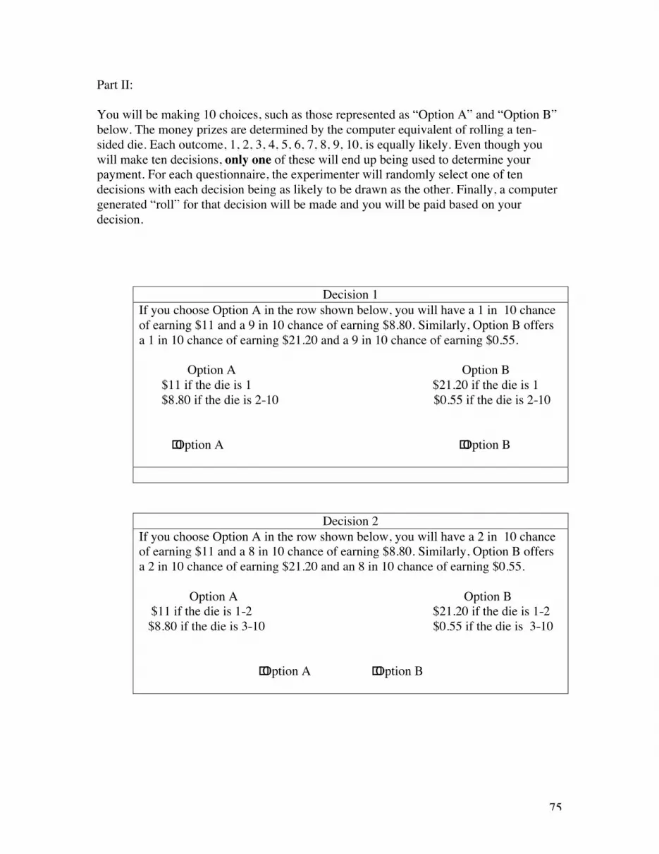
75

Part II:

You will be making 10 choices, such as those represented as “Option A” and “Option B”below. The money prizes are determined by the computer equivalent of rolling a ten-sided die. Each outcome, 1, 2, 3, 4, 5, 6, 7, 8, 9, 10, is equally likely. Even though youwill make ten decisions, only one of these will end up being used to determine yourpayment. For each questionnaire, the experimenter will randomly select one of tendecisions with each decision being as likely to be drawn as the other. Finally, a computergenerated “roll” for that decision will be made and you will be paid based on yourdecision.

Decision 1If you choose Option A in the row shown below, you will have a 1 in 10 chanceof earning $11 and a 9 in 10 chance of earning $8.80. Similarly, Option B offersa 1 in 10 chance of earning $21.20 and a 9 in 10 chance of earning $0.55.

Option A Option B $11 if the die is 1 $21.20 if the die is 1 $8.80 if the die is 2-10 $0.55 if the die is 2-10

� Option A � Option B

Decision 2If you choose Option A in the row shown below, you will have a 2 in 10 chanceof earning $11 and a 8 in 10 chance of earning $8.80. Similarly, Option B offersa 2 in 10 chance of earning $21.20 and an 8 in 10 chance of earning $0.55.

Option A Option B$11 if the die is 1-2 $21.20 if the die is 1-2$8.80 if the die is 3-10 $0.55 if the die is 3-10

� Option A � Option B

76

Decision 3If you choose Option A in the row shown below, you will have a 3 in 10 chanceof earning $11 and a 7 in 10 chance of earning $8.80. Similarly, Option B offers

a 3 in 10 chance of earning $21.20 and a 7 in 10 chance of earning $0.55.

Option A Option B$11 if the die is 1-3 $21.20 if the die is 1-3$8.80 if the die is 4-10 $0.55 if the die is 4-10

� Option A � Option B

Decision 4If you choose Option A in the row shown below, you will have a 4 in 10 chanceof earning $11 and a 6 in 10 chance of earning $8.80. Similarly, Option B offers

a 4 in 10 chance of earning $21.20 and a 6 in 10 chance of earning $0.55.

Option A Option B$11 if the die is 1-4 $21.20 if the die is 1-4$8.80 if the die is 5-10 $0.55 if the die is 5-10

� Option A � Option B

Decision 5If you choose Option A in the row shown below, you will have a 5 in 10 chanceof earning $11 and a 5 in 10 chance of earning $8.80. Similarly, Option B offers

a 5 in 10 chance of earning $21.20 and a 5 in 10 chance of earning $0.55.

Option A Option B$11 if the die is 1-5 $21.20 if the die is 1-5$8.80 if the die is 6-10 $0.55 if the die is 6-10

� Option A � Option B

77

Decision 6If you choose Option A in the row shown below, you will have a 6 in 10 chanceof earning $11 and a 4 in 10 chance of earning $8.80. Similarly, Option B offers

a 6 in 10 chance of earning $21.20 and a 4 in 10 chance of earning $0.55.

Option A Option B$11 if the die is 1-6 $21.20 if the die is 1-6$8.80 if the die is 7-10 $0.55 if the die is 7-10

� Option A � Option B

Decision 7If you choose Option A in the row shown below, you will have a 7 in 10 chanceof earning $11 and a 3 in 10 chance of earning $8.80. Similarly, Option B offers

a 7 in 10 chance of earning $21.20 and a 3 in 10 chance of earning $0.55.

Option A Option B$11 if the die is 1-7 $21.20 if the die is 1-7$8.80 if the die is 8-10 $0.55 if the die is 8-10

� Option A � Option B

Decision 8If you choose Option A in the row shown below, you will have a 8 in 10 chanceof earning $11 and a 2 in 10 chance of earning $8.80. Similarly, Option B offers

an 8 in 10 chance of earning $21.20 and a 2 in 10 chance of earning $0.55.

Option A Option B$11 if the die is 1-8 $21.20 if the die is 1-8$8.80 if the die is 9-10 $0.55 if the die is 9-10

� Option A � Option B

78

Decision 9If you choose Option A in the row shown below, you will have a 9 in 10 chanceof earning $11 and a 1 in 10 chance of earning $8.80. Similarly, Option B offers

a 9 in 10 chance of earning $21.20 and a 1 in 10 chance of earning $0.55.

Option A Option B$11 if the die is 1-9 $21.20 if the die is 1-9$8.80 if the die is 10 $0.55 if the die is 10

� Option A � Option B

Decision 10If you choose Option A in the row shown below, you will have a 10 in 10 chanceof earning $11 and a 0 in 10 chance of earning $8.80. Similarly, Option B offers

a 10 in 10 chance of earning $21.20 and a 0 in 10 chance of earning $0.55.

Option A Option B$11 if the die is 1-10 $21.20 if the die is 1-10

� Option A � Option B

79

Part III:In this section you will be asked to make a series of choices. In each scenario, there aretwo urns. Both will always contain 100 balls, each ball being either red or black. In eachscenario, you will know the exact number of black and red balls in one urn, but you willnot know the number of each color in the second urn, only that there are 100 balls in thesecond urn and every ball is either red or black. The balls are well mixed so that eachindividual ball is as likely to be drawn as any other.

For each questionnaire selected, the experimenter will randomly select one of the fivescenarios, with each scenario as likely to be drawn as any other. The experimenter willthen randomly select one of the two questions within the selected scenario, with eachquestion as likely to be selected as the other. Finally, if your questionnaire is selected, aball will be drawn on your behalf, with each ball as likely to be drawn as any other.

Finally, please note that there are no tricks in this experiment. While in each scenariothere is an urn for which you do not know the number of black and red balls, the numberof unknown balls of each type already has been selected at random and is on file with theWilliams College Department of Economics. Likewise, the pull of a ball from a chosenurn will truly be done at random via a process overseen by the Department of Economics.

Decision # 1Urn A: 100 balls: 50 red, 50 black

Urn C: 100 balls: ? red, ? blackIf I were to give you $10 if you pulled a red ball on your first try, from which urn

would you choose to draw?

� Urn A � Urn C

If I were to give you $10 if you pulled a black ball on your first try, from whichurn would you choose to draw?

� Urn A � Urn C

Decision # 2Urn D: 100 balls: 40 red, 60 black

Urn E: 100 balls: ? red, ? blackIf I were to give you $10 if you pulled a red ball on your first try, from which urn

would you choose to draw?

� Urn D � Urn E

If I were to give you $10 if you pulled a black ball on your first try, from whichurn would you choose to draw?

� Urn D � Urn E

80

Decision # 3Urn F: 100 balls: 30 red, 70 blackUrn G: 100 balls: ? red, ? black

If I were to give you $10 if you pulled a red ball on your first try, from which urnwould you choose to draw?

� Urn F � Urn G

If I were to give you $10 if you pulled a black ball on your first try, from whichurn would you choose to draw?

� Urn F � Urn G

Decision # 4Urn H: 100 balls: 20 red, 80 black

Urn I: 100 balls: ? red, ? blackIf I were to give you $10 if you pulled a red ball on your first try, from which urn

would you choose to draw?

� Urn H � Urn I

If I were to give you $10 if you pulled a black ball on your first try, from whichurn would you choose to draw?

� Urn H � Urn I

Decision # 5Urn J: 100 balls: 10 red, 90 blackUrn K: 100 balls: ? red, ? black

If I were to give you $10 if you pulled a red ball on your first try, from which urnwould you choose to draw?

� Urn J � Urn K

If I were to give you $10 if you pulled a black ball on your first try, from whichurn would you choose to draw?

� Urn J � Urn K

81

PART IV:

Please answer the below questions according to your own feelings, rather than how youthink "most people" would answer. Please be as honest and accurate as you canthroughout, there is no right or wrong answer. Also, please try not to let your response toone statement influence your responses to other statements. Think about each statementon its own.

A = I agree a lot B = I agree a little C = I neither agree nor disagree D = I disagree a little E = I disagree a lot

In uncertain times, I usually expect the best. A B C D E

It’s easy for me to relax. A B C D E

If something can go wrong, it will. A B C D E

I’m always optimistic about the future. A B C D E

I enjoy my friends a lot. A B C D E

It’s important for me to keep busy. A B C D E

I hardly ever expect things to go my way. A B C D E

I don’t get upset too easily A B C D E

I rarely count on good things happening to me. A B C D E

Overall, I expect more good things to happen to me thanbad. A B C D E

82

PERSONAL INFORMATION:

NAME:

EMAIL ADDRESS:

83

Version 2:

Welcome to this experiment on decision-making and thank you for being here. You willbe compensated for your participation in the experiment, though the exact amount youwill receive will depend on the choices you make, and on random chance (asexplained below). Please pay careful attention to these instructions, as a significantamount of money is at stake.

Information about the choices that you make during the experiment will be kept strictlyconfidential. In order to maintain privacy and confidentiality, please do not speak toanyone during the experiment and please do not discuss your choices with anyone evenafter the conclusion of the experiment.

This experiment has four parts. First, you will be asked to make a series of decisionsregarding charitable donations. Second, you will be asked to make a series of decisionsbetween two lotteries based on the rolling of a die (a computer will conduct the actualrandomization). Then you will be asked to make a series of decisions based on drawing aball from an urn. Finally, you will be asked a series of questions with which you willeither agree or disagree with along a scale. More detailed instructions will follow in eachsection.

Part I:

Today you received a show up fee of X dollars. You will now have the opportunity toshare part or all of that show up fee with one or both of two charities. You may donate asmuch or as little of your show up fee to each of these charities as you wish. Pleaseindicate below the amount you would like to donate and sign where indicated.

3. Oxfam, a nonprofit organization that works to minimize poverty through reliefand development work in Africa. The experimenter will match any amount thatyou donate to Oxfam.

4. A nonprofit organization that works to help victims of natural disasters. Theexperimenter will match any amount that you donate to this organization.

84

Version 3:

Welcome to this experiment on decision-making and thank you for being here. You willbe compensated for your participation in the experiment, though the exact amount youwill receive will depend on the choices you make, and on random chance. Even thoughyou will make twenty decisions, only one of these will end up being used to determineyour payment. Please pay careful attention to these instructions, as a significant amountof money is at stake.

Information about the choices that you make during the experiment will be kept strictlyconfidential. In order to maintain privacy and confidentiality, please do not speak toanyone during the experiment and please do not discuss your choices with anyone evenafter the conclusion of the experiment.

This experiment has four parts. First, you will be asked to make a series of decisionsregarding charitable donations. In the second and third sections, you will be asked tomake a series of choices between options, where the outcome of each option is not knowwith certainty. Finally, you will be asked a series of questions with which you will eitheragree or disagree with along a scale. More detailed instructions will follow in eachsection.

Part I:

Today you received four envelopes: a “Start” envelope, a “Me” envelope, a “1” envelope,and a “2” envelope. In the start envelope you will find ten $1 bills and ten dollar-sizepieces of blank paper. You will now have the opportunity to share part or all of the $10with one or both of two charities. Any money that you donate to either charity will bematched; meaning every dollar you donate will result in the charity receiving two dollars.You may donate as much or as little of the $10 to each of these charities as you wish byplacing dollar bills in the corresponding envelopes. At the end of the experiment, youwill keep the “Me” envelope and any dollar bills you place in that envelope.

5. Envelope 1: A nonprofit organization that works to alleviate poverty in Africa.

6. Envelope 2: Habitat for Humanity, a nonprofit organization that builds home forthose in need which has been instrumental in Hurricane Katrina relief efforts inthe United States.

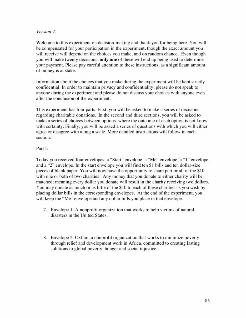
85

Version 4:

Welcome to this experiment on decision-making and thank you for being here. You willbe compensated for your participation in the experiment, though the exact amount youwill receive will depend on the choices you make, and on random chance. Even thoughyou will make twenty decisions, only one of these will end up being used to determineyour payment. Please pay careful attention to these instructions, as a significant amountof money is at stake.

Information about the choices that you make during the experiment will be kept strictlyconfidential. In order to maintain privacy and confidentiality, please do not speak toanyone during the experiment and please do not discuss your choices with anyone evenafter the conclusion of the experiment.

This experiment has four parts. First, you will be asked to make a series of decisionsregarding charitable donations. In the second and third sections, you will be asked tomake a series of choices between options, where the outcome of each option is not knowwith certainty. Finally, you will be asked a series of questions with which you will eitheragree or disagree with along a scale. More detailed instructions will follow in eachsection.

Part I:

Today you received four envelopes: a “Start” envelope, a “Me” envelope, a “1” envelope,and a “2” envelope. In the start envelope you will find ten $1 bills and ten dollar-sizepieces of blank paper. You will now have the opportunity to share part or all of the $10with one or both of two charities. Any money that you donate to either charity will bematched; meaning every dollar you donate will result in the charity receiving two dollars.You may donate as much or as little of the $10 to each of these charities as you wish byplacing dollar bills in the corresponding envelopes. At the end of the experiment, youwill keep the “Me” envelope and any dollar bills you place in that envelope.

7. Envelope 1: A nonprofit organization that works to help victims of naturaldisasters in the United States.

8. Envelope 2: Oxfam, a nonprofit organization that works to minimize povertythrough relief and development work in Africa, committed to creating lastingsolutions to global poverty, hunger and social injustice.