SEQUENTIAL TWO-PLAYER GAMES WITH AMBIGUITY1

Jürgen Eichberger and David KelseyAlfred Weber Institut Department of Economics

Universität Heidelberg The University of BirminghamGermany United Kingdom

February 2004

Abstract

If players’ beliefs are strictly non-additive, the Dempster-Shafer updating rule can be

used to define beliefs off the equilibrium path. We define an equilibrium concept in se-

quential two-person games where players update their beliefs with the Dempster-Shafer

updating rule. We show that in the limit as uncertainty tends to zero, our equilibrium ap-

proximates Bayesian Nash equilibrium. We argue that our equilibrium can be used to define

a refinement of Bayesian Nash equilibrium by imposing context-dependent constraints on

beliefs under uncertainty.

1 Financial assistancefrom theESRC senior research fellowship scheme, award no. H52427502595, the School

of Social Science at the University of Birmingham, the Department of Economics at the University of Melbourne

and The British Academy is gratefully acknowledged. For comments we would like to thank Simon Grant, Hans

Haller, Youngse Kim, Bart Lipman, Frank Milne, Shasi Nandeibam, Hyun Shin, Peter Sinclair, Willy Spanjers,

Martin Summer, Peter Wakker and participants in seminars at Queen’s university, the universities of Melbourne

and Birmingham, the Econometric Society World meetings in Tokyo 1995 and the ESRC game theory workshop,

Kenilworth 1997. We thank two anonymous referees of this journal for detailed comments which helped to im-

prove the the final version.

1

JEL Classification: C72, D81

Keywords: Uncertainty-aversion, capacity, Dempster-Shafer rule, bargaining, signalling

game.

Running Head: SEQUENTIAL GAMES WITH AMBIGUITY

Address:

Professor Dr. Jürgen Eichberger

Wirtschaftstheorie I

Alfred Weber Institut

RUPRECHT-KARLS-UNIVERSITÄT HEIDELBERG

Grabengasse 14

D-69117 HEIDELBERG

GERMANY

2

1. INTRODUCTION

Economists have made a distinctionbetween risk (where probabilities are objectively known)

and ambiguity (where probabilities are unknown). Until recently it was not clear how to

model this formally. Schmeidler (1989) has proposed an axiomatic decision theory, which

is able to model ambiguity. In this theory, the decision-maker’s beliefs are represented by a

capacity (non-additive subjective probability) and (s)he is modelled as maximising the ex-

pected value of utility with respect to the capacity. Ambiguity is represented by strictly non-

additive capacities. The expectation is expressed as a Choquet integral (Choquet, 1953-4).

Schmeidler’s theory will henceforth be referred to as Choquet expected utility (CEU).

A number of researchers have applied CEU (or related theories) to games2. Most of

these papers consider strategic (normal) form games. Lo (1999) suggests an equilibrium

concept for extensive form games under ambiguity. Since he uses the related multiple-prior

expected utility theory to model ambiguity, he discusses a number of conceptual problems

which arise in the context of dynamic games if players face strategic ambiguity. The paper

contains many instructive examples but no general theorems about existence of equilibrium

if players face ambiguity.

Approaching the problem of extensive form games in a very general way, Lo (1999)

cannot exploit one of the strengths of non-additive probabilities, namely that unlike additive

probabilities, they can be updated after events with a capacity value of zero. In the present

paper, we apply CEU to sequential two-player games. This class of extensive form games

2 See Dow and Werlang (1994), Eichberger and Kelsey (2000), Hendon et al. (1994), Klibanoff (1996), Lo

(1996) and Marinacci (2000).

3

comprises many important game-theoretic models in economics such as signalling games,

two-stage industrial organisation models or bargaining problems. Restricting ourself to

this class of games allows us to ignore some of the consistency problems encountered in

Lo (1999).

In extensive form games, updating of beliefs on newly acquired information is impor-

tant. If beliefs are represented by additive probability distributions, then Bayesian updating

is the natural method to incorporate the information obtained from the observed moves of

the opponents. Bayesian updating however is possible only at information sets which have

a positive probability of being reached. As is well-known, play at information sets off the

equilibrium path can have a major effect on the equilibrium itself. Thus it is important to

determine players’ beliefs at such information sets. Because Bayesian updating puts no

restrictions on such beliefs, a multiplicity of equilibria is compatible with Bayesian beliefs.

Games with incomplete information are usually plagued by a large number of Bayes-

Nash equilibria. Signalling games in particular have typically an excessively large number

of equilibria because the signal space is large compared to the type space, which implies

that most actions will not be observed in equilibrium. The multiplicity of equilibria depends

on the lack of constraints on out-of-equilibrium strategies. There is a huge literature in

game-theory which tries to impose further constraints on beliefs by additional rules about

how a player should interpret out-of-equilibrium moves in equilibrium. Such constraints

on beliefs refine the set of Bayes-Nash equilibria. Compare Mailath (1992) for a survey

of refinements in the context of signalling games. Most refinements have been based on

forward or backward induction arguments. A common criticism of such arguments is that, if

4

the initial situation is indeed an equilibrium, then players should conclude from a deviation

that the opponent is not rational or does not understand the structure of the game.

In this paper, we propose a definition of equilibrium where players have non-additive

beliefs and use an updating rule proposed by Dempster and Shafer in the literature for ca-

pacities. This equilibrium notion comprises Bayes-Nash equilibrium as a special case. The

Dempster-Shafer updating rule, which is part of our equilibrium concept, has well-defined

updated capacities off the equilibrium path as long as there is ambiguity. Capacities can

be further constrained by adequate assumptions about beliefs without affecting consistency

of beliefs in an equilibrium under ambiguity. Hence, there is room to put constraints on

beliefs which may be specific to situation one wants to model. For example, one can ex-

ogenously determine the degree of ambiguity or one can restrict beliefs to agree with an

additive prior distribution, if one wants to model a situation where players are completely

confident about the distribution of types but ambiguous about their opponents’ strategic be-

haviour. It is possible to control for the ambiguity of a situation in experiments in order to

see how it affects decision behaviour. For individual decision situations, such experiments

have been performed (Camerer and Weber, 1992). There are few experiments so far, which

focus on strategic ambiguity, but we are confident that such tests can be conducted.

One can parametrise the notion of ambiguity and demonstrate existence of equilibrium

for any exogenously determined level of ambiguity. This opens up the possibility to study

sequences of equilibria under ambiguity which converge to a Bayesian equilibrium as ambi-

guity vanishes. Assumptions about beliefs under ambiguity will determine which Bayesian

equilibrium will be selected. An interesting aspect of this approach is, even in a Bayesian

5

equilibrium, beliefs off the equilibrium path may be represented by capacities which are

not additive. The greater freedom of modelling beliefs under ambiguity provides a novel

and useful modelling device for economic applications.

In section 2 we introduce the CEU model and demonstrate some properties of CEU

and the Dempster–Shafer updating rule. Section 3 introduces our solution concept for two-

stage games under ambiguity and relates it to some existing solution concepts. Section 4

studies limits of sequences of equilibria as ambiguity vanishes. We show that ambiguous

beliefs can select among Bayesian equilibria. Section 6 concludes the paper. All proofs are

gathered in an appendix.

2. CEU PREFERENCES AND DS-UPDATING

In this section we consider a finite set S of states of nature. A subset of S is referred to

as an event. The set of possible outcomes or consequences is denoted by X . An act is a

function from S to X . The space of all acts is denoted by A(S) := faj a : S ! Xg. The

decision-maker’s preferences over A(S) are denoted by <.

A capacity or non-additive probability on S is a real-valued function º on the subsets

of S; which satisfies the following properties:

(i) A µ B implies º (A) 6 º (B) ;

(ii) º (?) = 0; º (S) = 1:

The capacity is said to be convex if for all A; B µ S; º(A[B) > º(A)+º(B)¡º(A\

B): Representing beliefs by a convex capacity is compatible with experimental evidence

(see Camerer und Weber, 1992) and is commonly used in applications of CEU to model

ambiguity averse behaviour. We shall assume that all capacities are convex.

6

We shall use capacities to represent the beliefs of players. In game-theoretic applica-

tions, the opponents’ strategy combinations will be the relevant states for a player. It is

possible to define an expected value with respect to a capacity to be a Choquet integral

(Choquet, 1955).

For any function Á : S ! Rand any outcome x 2 X let B(xjÁ) := fs 2 S : Á (s) > xg

be the event in which Á is greater than or equal to x: Similarly, denote by B(xjÁ) :=

fs 2 S : Á (s) > xg the event in which Á produces a strictly greater outcome than x: The

Choquet integral of Á with respect to the capacity º is defined asZ

Á dº :=nX

x2Á(S)

x ¢ [º (B(xjÁ)) ¡ º (B(xjÁ))];(1)

where the summation is over the range of the act, Á(S) := fx 2 X j 9 s 2 S; Á(s) = xg:

We shall assume that preferences may be represented by Choquet expected utility (CEU)

with respect to a capacity, i.e.

a < b ,Z

u(a(s))dº (s) >Z

u (b (s)) dº (s) :

Such preferences have been axiomatised by Gilboa (1987) and Sarin and Wakker (1992).

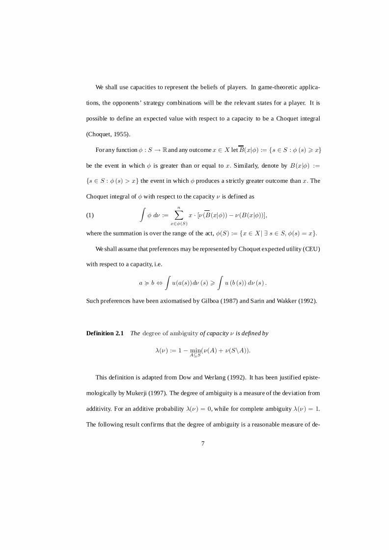
Definition 2.1 The degree of ambiguity of capacity º is defined by

¸(º ) := 1 ¡ minAµS

(º(A) + º(SnA)):

This definition is adapted from Dow and Werlang (1992). It has been justified episte-

mologically by Mukerji (1997). The degree of ambiguity is a measure of the deviation from

additivity. For an additive probability ¸(º ) = 0, while for complete ambiguity ¸(º ) = 1.

The following result confirms that the degree of ambiguity is a reasonable measure of de-

7

viation from additivity, for convex capacities3.

Lemma 2.2 If a convex capacity º has zero degree of ambiguity then it is additive.

2.1 The support of a capacity

In game theory, players are assumed to maximise their expected payoffs. Strategy choices

are considered in equilibrium if beliefs are consistent with actual behaviour. The strongest

form of consistency, Nash equilibrium, requires players’ beliefs to coincide with their actual

behaviour. In an alternative and equivalent definition of Nash equilibrium the strategies in

the support of the opponents’ beliefs about a player’s behaviour must be best responses

of that player. In other words, players expect their opponents to play only best-response

strategies.

If decision makers’ ambiguity is modelled by capacities then there are several concepts

of a support which all coincide with the usual notion of support in the case of additive

capacities. In this paper we will use the following definition.

Definition 2.3 A support of a capacity º is an event A µ S such that º (SnA) = 0 and

º(SnB) > 0; for all events B ½ A:

This definition of the support is due to Dow and Werlang (1994). Above we define the

support of a capacity to be a minimal set whose complement has a capacity value of zero.

This is equivalent to the usual definition of support (i.e. a minimal set of probability one)

for an additive capacity but will generally yield a smaller set if the capacity is not additive.

3 The lemma is false if convexity is not assumed. Acounter-examplewould be the class of symmetric capacities

studied by Gilboa (1989) and Nehring (1994).

8

With this support notion every capacity has a support. However it has been criticised

because the support is not necessarily unique and states outside the support may affect

decision making if a bad outcome occurs on them. In Eichberger and Kelsey (2001) we

provide an extensive discussion of various support notions for capacities suggested in the

literature4. In particular, we show that the support is unique if and only if one requires in

addition º(B) > 0; for all events B in the support. Adding this requirement to Definition

2.3 guarantees a unique support but there are convex capacities for which no such support

exists. In game-theoretic applications, the lack of uniqueness poses no problem because

we show the existence of an equilibrium in which beliefs have a unique support. Moreover,

our results and examples all have unique supports, which satisfy this additional restriction.

More substantial is the objection to Definition 2.3 that states outside the support are not

Savage-null. An event E is Savage-null if outcomes on E never affect a decision, i.e. if

aEc » bEc for all acts a; b; c; where aEc denotes an act which yields a(s) for all states in

E and c(s) in all other states. We believe that this argument is not appropriate in game-

theoretic applications. We will argue this case below in context with the game-theoretic

equilibrium concept, which we advance in this paper.

2.2 CEU preferences and DS-updating

In sequential games players may receive information about the opponents by observing their

moves in earlier stages of the game. In particular in signalling games, second-stage players

will try to infer information about characteristics of their opponents from the signals which

they receive. It is therefore necessary to specify a rule for how to revise beliefs represented

4 Haller (2000), Marinacci (2000) and in particular Ryan (1998) discuss and argue for other support notions.

9

by capacities in the light of new information.

If beliefs are additive, Bayes’ rule is the unique updating rule which maintains additiv-

ity. As in the case of the support, with non-additive capacities there are several updating

procedures, which all coincide with Bayesian updating in the case of additivity. Gilboa and

Schmeidler (1993) provide an exposition and an axiomatic treatment from a behavioural

perspective. In this paper we choose the Dempster-Shafer belief revision rule (see Shafer,

1976).

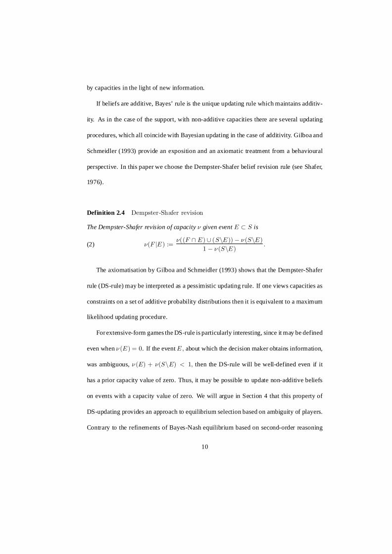
Definition 2.4 Dempster-Shafer revision

The Dempster-Shafer revision of capacity º given event E ½ S is

º(F jE) :=º((F \ E) [ (SnE)) ¡ º (SnE)

1 ¡ º (SnE):(2)

The axiomatisation by Gilboa and Schmeidler (1993) shows that the Dempster-Shafer

rule (DS-rule) may be interpreted as a pessimistic updating rule. If one views capacities as

constraints on a set of additive probability distributions then it is equivalent to a maximum

likelihood updating procedure.

For extensive-form games the DS-rule is particularly interesting, since it may be defined

even when º (E) = 0. If the event E; about which the decision maker obtains information,

was ambiguous, º (E) + º(SnE) < 1; then the DS-rule will be well-defined even if it

has a prior capacity value of zero. Thus, it may be possible to update non-additive beliefs

on events with a capacity value of zero. We will argue in Section 4 that this property of

DS-updating provides an approach to equilibrium selection based on ambiguity of players.

Contrary to the refinements of Bayes-Nash equilibrium based on second-order reasoning

10

about out-of-equilibrium moves, which dominate the literature, ambiguity-related refine-

ments can be given a behavioural content which is independent of the equilibrium notion.

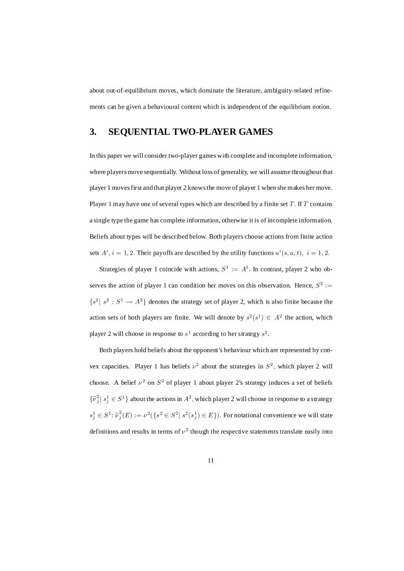
3. SEQUENTIAL TWO-PLAYER GAMES

In this paper we will consider two-player games with complete and incomplete information,

where players move sequentially. Without loss of generality, we will assume throughout that

player 1 moves first and that player 2 knows the move of player 1 when she makes her move.

Player 1 may have one of several types which are described by a finite set T: If T contains

a single type the game has complete information, otherwise it is of incomplete information.

Beliefs about types will be described below. Both players choose actions from finite action

sets Ai; i = 1; 2: Their payoffs are described by the utility functions ui(s; a; t); i = 1; 2:

Strategies of player 1 coincide with actions, S1 := A1: In contrast, player 2 who ob-

serves the action of player 1 can condition her moves on this observation. Hence, S2 :=

fs2j s2 : S1 ! A2g denotes the strategy set of player 2, which is also finite because the

action sets of both players are finite. We will denote by s2(s1) 2 A2 the action, which

player 2 will choose in response to s1 according to her strategy s2:

Both players hold beliefs about the opponent’s behaviour which are represented by con-

vex capacities. Player 1 has beliefs º2 about the strategies in S2; which player 2 will

choose. A belief º 2 on S2 of player 1 about player 2’s strategy induces a set of beliefs

feº 2j j s1

j 2 S1g about the actions in A2; which player 2 will choose in response to a strategy

s1j 2 S1: eº 2

j (E) := º 2(fs2 2 S2j s2(s1j ) 2 Eg): For notational convenience we will state

definitions and results in terms of º 2 though the respective statements translate easily into

11

statements about the set of beliefs about actions feº2j j s1

j 2 S1g:

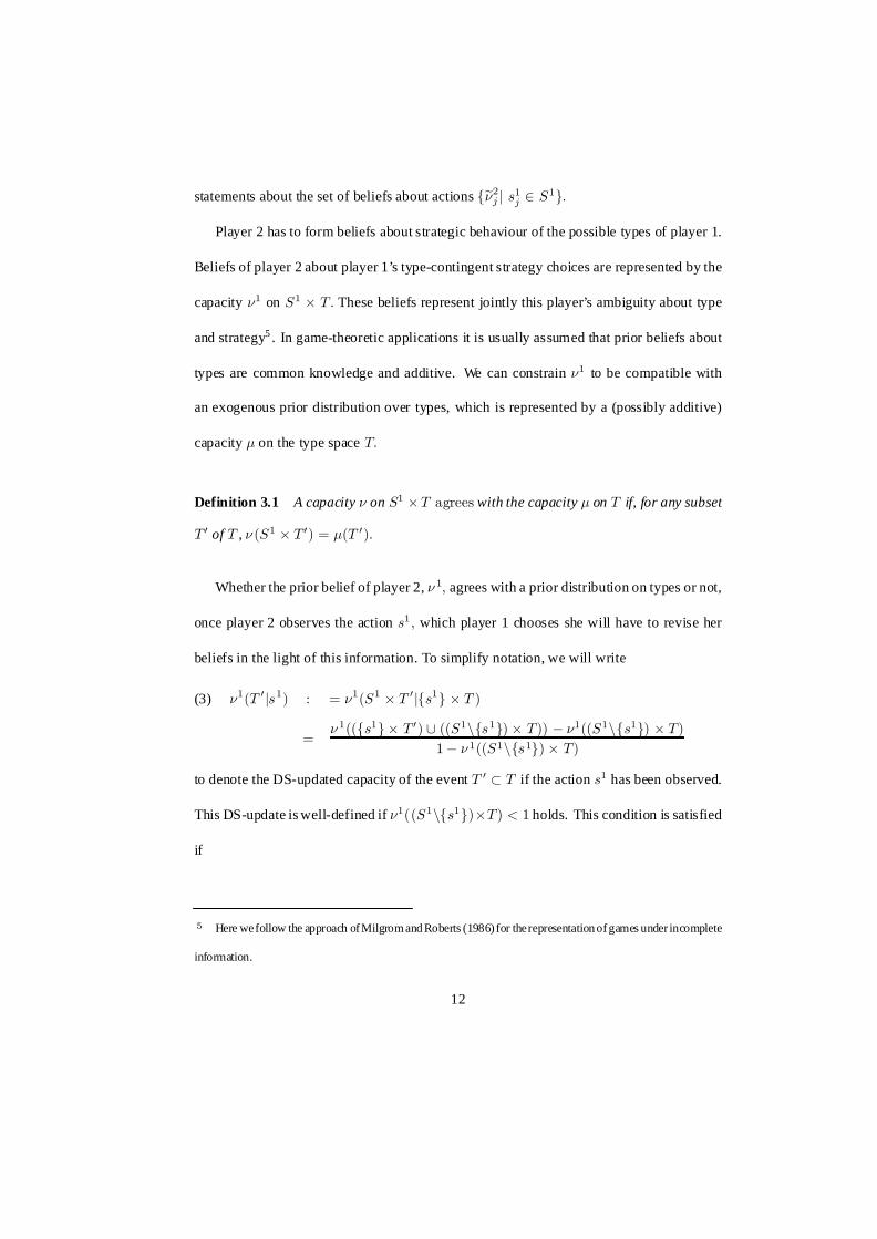
Player 2 has to form beliefs about strategic behaviour of the possible types of player 1.

Beliefs of player 2 about player 1’s type-contingent strategy choices are represented by the

capacity º1 on S1 £ T: These beliefs represent jointly this player’s ambiguity about type

and strategy5 . In game-theoretic applications it is usually assumed that prior beliefs about

types are common knowledge and additive. We can constrain º1 to be compatible with

an exogenous prior distribution over types, which is represented by a (possibly additive)

capacity ¹ on the type space T:

Definition 3.1 A capacity º on S1 £T agrees with the capacity ¹ on T if, for any subset

T 0 of T , º (S1 £ T 0) = ¹(T 0):

Whether the prior belief of player 2, º 1; agrees with a prior distribution on types or not,

once player 2 observes the action s1; which player 1 chooses she will have to revise her

beliefs in the light of this information. To simplify notation, we will write

º1(T 0js1) : = º1(S1 £ T 0jfs1g £ T )(3)

=º 1((fs1g £ T 0) [ ((S1nfs1g) £ T)) ¡ º1((S1nfs1g) £ T)

1 ¡ º 1((S1nfs1g) £ T)

to denote the DS-updated capacity of the event T 0 ½ T if the action s1 has been observed.

This DS-update is well-defined if º1((S1nfs1g)£T) < 1 holds. This condition is satisfied

if

5 Here wefollow the approach ofMilgrom and Roberts (1986) for therepresentation ofgames under incomplete

information.

12

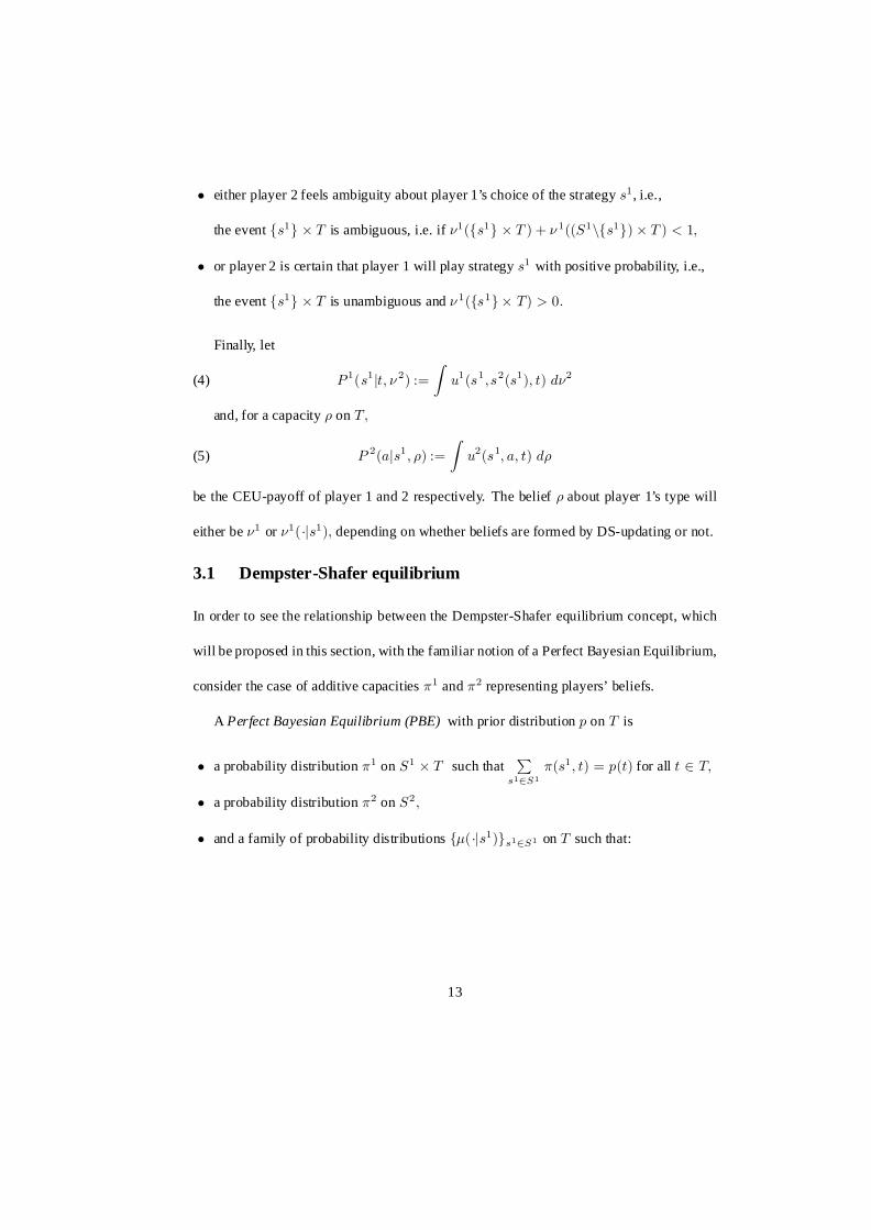
² either player 2 feels ambiguity about player 1’s choice of the strategy s1, i.e.,

the event fs1g £ T is ambiguous, i.e. if º1(fs1g £ T ) + º 1((S1nfs1g) £ T ) < 1;

² or player 2 is certain that player 1 will play strategy s1 with positive probability, i.e.,

the event fs1g £ T is unambiguous and º 1(fs1g £ T) > 0:

Finally, let

P 1(s1jt; º 2) :=Z

u1(s1;s2(s1); t) dº2(4)

and, for a capacity ½ on T;

P 2(ajs1; ½) :=Z

u2(s1; a; t) d½(5)

be the CEU-payoff of player 1 and 2 respectively. The belief ½ about player 1’s type will

either be º1 or º1(¢js1); depending on whether beliefs are formed by DS-updating or not.

3.1 Dempster-Shafer equilibrium

In order to see the relationship between the Dempster-Shafer equilibrium concept, which

will be proposed in this section, with the familiar notion of a Perfect Bayesian Equilibrium,

consider the case of additive capacities ¼1 and ¼2 representing players’ beliefs.

A Perfect Bayesian Equilibrium (PBE) with prior distribution p on T is

² a probability distribution ¼1 on S1 £ T such thatP

s12S1¼(s1; t) = p(t) for all t 2 T;

² a probability distribution ¼2 on S2;

² and a family of probability distributions f¹(¢js1)gs12S1 on T such that:

13

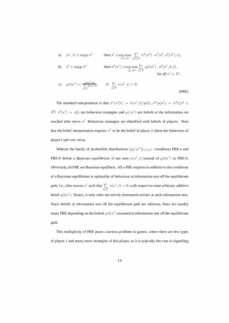
a) (s1; t) 2 supp ¼1 then s1 2arg maxes12S1

Ps22S2

¼2(s2) ¢ u1(es1; s2(es1); t);

b) s2 2 supp ¼2 then s2(s1) 2arg maxea2A2

Pt2T

¹(tjs1) ¢ u2(s1;ea; t);

for all s1 2 S1;

c) ¹(tjs1) = ¼(s1;t)Pt2T

¼(s1 ;t) ifPt2T

¼ (s1; t) > 0:

(PBE)

The standard interpretation is that ¼1(s1jt) := ¼(s1; t)=p(t); ¼2(ajs1) := ¼2(fs2 2

S2j s2(s1) = ag) are behaviour strategies and ¹(¢js1) are beliefs at the information set

reached after move s1: Behaviour strategies are identified with beliefs of players. Note

that the belief interpretation requires ¼1 to be the belief of player 2 about the behaviour of

player1 and vice versa.

Without the family of probability distributions f¹(¢js1)gs12S1 ; conditions PBE-a and

PBE-b define a Bayesian equilibrium if one uses ¼(s1; t) instead of ¹(tjs1) in PBE-b.

Obviously, all PBE are Bayesian equilibria. All a PBE requires in addition to the conditions

of a Bayesian equilibrium is optimality of behaviour at information sets off the equilibrium

path, i.e., after moves s1 such thatPt2T

¼(s1; t) = 0; with respect to some arbitrary additive

belief ¹(tjs1): Hence, it only rules out strictly dominated actions at such information sets.

Since beliefs at information sets off the equilibrium path are arbitrary, there are usually

many PBE depending on the beliefs ¹(tjs1) assumed at information sets off the equilibrium

path.

This multiplicity of PBE poses a serious problem in games, where there are few types

of player 1 and many more strategies of this player, as it is typically the case in signalling

14

games. The literature is therefore particularly rich in refinements for signalling games.

Mailath (1992) provides a good survey of the refinements applied in the context of sig-

nalling games. We show below in Example 4.2 howwith ambiguity aversion, a quite natural

assumption on beliefs can reduce this multiplicity of equilibria.

Games in strategic form where the beliefs of players are represented by capacities have

been studied by Dow and Werlang (1994), Marinacci (2000) and Eichberger and Kelsey

(2000). In the strategic form, beliefs (º1; º2) form an equilibria under uncertainty if these

beliefs have supports containing only pure strategies which are optimal for the respective

player given these beliefs.

In this paper we study sequential two-player games where the action of player 1 con-

veys information to player 2. This requires a reformulation of the equilibrium concept.

In contrast to the equilibrium notion in the strategic form, we will require that player 2’s

strategy consists of actions that are optimal at each information set, i.e. after observing the

action of player 1.

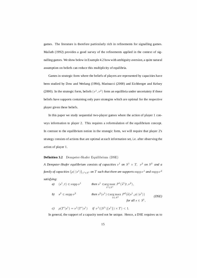
Definition 3.2 Dempster-Shafer Equilibrium (DSE)

A Dempster-Shafer equilibrium consists of capacities º1 on S1 £ T; º2 on S2 and a

family of capacities f½(¢js1)gs12S1 on T such that there are supports suppº 1 and suppº 2

satisfying:

a) (s1; t) 2 supp º1 then s1 2arg maxes12S1

P 1(es1jt; º2);

b) s2 2 supp º2 then s2(s1) 2arg maxea2A2

P 2(eajs1; ½(¢js1))

for all s 2 S1;

c) ½(T 0js1) = º1(T 0js1) if º 1((S1nfs1g) £ T ) < 1:

(DSE)

In general, the support of a capacity need not be unique. Hence, a DSE requires us to

15

specify a set of beliefs and some associated support. In most applications the capacities

considered will have a unique support and this seemingly arbitrary choice of support for a

given capacity poses no problem6 . Condition DSE-a of Definition 3.2 guarantees that only

optimal type-contingent strategies of player 1 will be included in the support of player 2’s

beliefs. Similarly, by condition DSE-b there are only strategies in the support of player 1’

beliefs which prescribe optimal behaviour after a strategy of player 1. We call the equilib-

rium a Dempster-Shafer equilibrium (DSE) because, according to DSE-c, beliefs of player

2 about the type of player 1 are obtained by the DS-updating rule.

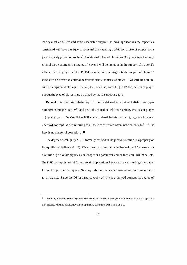
Remark: A Dempster-Shafer equilibrium is defined as a set of beliefs over type-

contingent strategies (º 1; º2) and a set of updated beliefs after strategy choices of player

1, f½(¢js1)gs12S1 : By Condition DSE-c the updated beliefs f½(¢js1)gs12S1 are however

a derived concept. When referring to a DSE we therefore often mention only (º1; º 2); if

there is no danger of confusion.

The degree of ambiguity ¸(º i); formally defined in the previous section, is a property of

the equilibrium beliefs (º1; º2). We will demonstrate below in Proposition 3.5 that one can

take this degree of ambiguity as an exogenous parameter and deduce equilibrium beliefs.

The DSE concept is useful for economic applications because one can study games under

different degrees of ambiguity. Nash equilibrium is a special case of an equilibrium under

no ambiguity. Since the DS-updated capacity ½(¢js1) is a derived concept its degree of

6 There are, however, interesting cases where supports are not unique, yet where there is only one support for

each capacity which is consistent with the optimality conditions DSE-a and DSE-b.

16

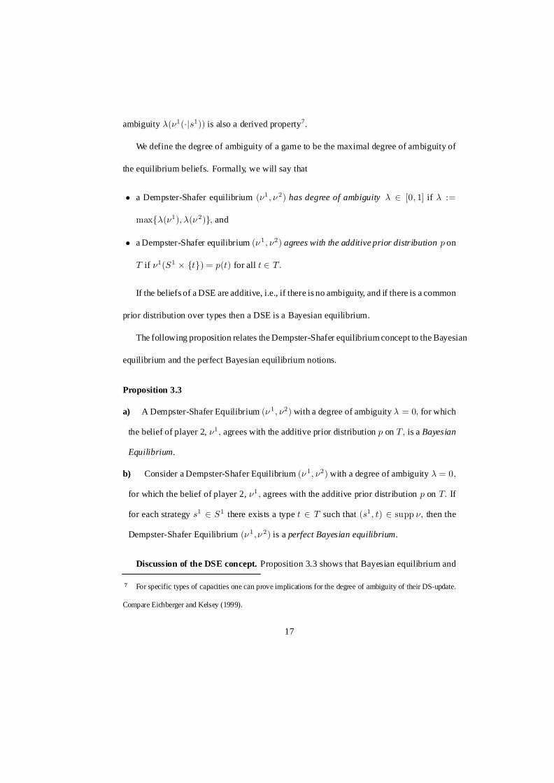
ambiguity ¸(º1(¢js1)) is also a derived property7.

We define the degree of ambiguity of a game to be the maximal degree of ambiguity of

the equilibrium beliefs. Formally, we will say that

² a Dempster-Shafer equilibrium (º1; º 2) has degree of ambiguity ¸ 2 [0; 1] if ¸ :=

maxf¸(º1); ¸(º 2)g; and

² a Dempster-Shafer equilibrium (º 1; º2) agrees with the additive prior distribution p on

T if º1(S1 £ ftg) = p(t) for all t 2 T:

If the beliefs of a DSE are additive, i.e., if there is no ambiguity, and if there is a common

prior distribution over types then a DSE is a Bayesian equilibrium.

The following proposition relates the Dempster-Shafer equilibrium concept to the Bayesian

equilibrium and the perfect Bayesian equilibrium notions.

Proposition 3.3

a) A Dempster-Shafer Equilibrium (º 1; º2) with a degree of ambiguity ¸ = 0; for which

the belief of player 2, º1; agrees with the additive prior distribution p on T; is a Bayesian

Equilibrium.

b) Consider a Dempster-Shafer Equilibrium (º 1; º2) with a degree of ambiguity ¸ = 0;

for which the belief of player 2, º1; agrees with the additive prior distribution p on T: If

for each strategy s1 2 S1 there exists a type t 2 T such that (s1; t) 2 supp º; then the

Dempster-Shafer Equilibrium (º 1;º 2) is a perfect Bayesian equilibrium.

Discussion of the DSE concept. Proposition 3.3 shows that Bayesian equilibrium and

7 For specific types of capacities one can prove implications for the degree of ambiguity of their DS-update.

Compare Eichberger and Kelsey (1999).

17

perfect Bayesian equilibrium are special cases of a DSE if there is no ambiguity. There

is mounting experimental evidence that Nash equilibrium and its refinements do not yield

good predictions of actual behaviour in all games. Situations in which one finds consistent

deviations from the Nash equilibrium hypothesis include bargaining, e.g. the ultimatum

bargaining experiments (Roth, 1995), coordination problems (Ochs, 1995), public goods

provision (Ledyard, 1995), and signalling games (Brandts and Holt, 1992 and 1993). These

findings pose a challenge to theory and call for the investigation of modified equilibrium

concepts. Some of these anomalies can be explained by altruistic preferences, e.g. in the

cases of public goods and bargaining. Even in these cases however, it is difficult to account

for all the observed phenomena by modifying preferences alone.

The approach we propose in this paper focuses on ambiguity about the behaviour of the

opponent players. We do not give up the idea that players maximise their expected payoff

but we investigate how ambiguity about the strategic behaviour of opponents affects the

equilibria of games. Ambiguity about the opponents’ behaviour may arise by a number of

reasons.

Traditional game theory maintains that players deduce beliefs about the opponents’ be-

haviour from firm knowledge about the preferences of opponents. In games with incom-

plete information one replaces knowledge about other players’ payoffs, with knowledge

about the probability distribution over possible types of payoffs. Though logically sound

and completely consistent, modelling games of incomplete information by probability dis-

tributions over type spaces assumes that players have extremely high computational abili-

ties.

18

Ambiguity about the strategic behaviour of the opponent players reflects the difficulty

of settling one’s beliefs firmly on a particular probability distribution over types and their

behaviour. This does not imply that players do not care about the motivation of the oppo-

nents or that they do not consider the possibility of different types of opponents. It means

however that their behaviour may be influenced by the fact that they do not feel certain

about such inferences.

Ambiguous beliefs represented by capacities, allow us to model players who hold and

process information about their opponents in order to predict their behaviour but who, de-

pending on the situation, may feel more or less certain about these predictions. If ambiguity

is about two or more possible characteristics of an opponent then beliefs should be modelled

by a capacity over the relevant type space, if ambiguity concerns the correct description

of the situation in general it is best modelled by ambiguity about the opponents’ strategy

choices. Equilibrium concepts for ambiguous players, like the DSE suggested here, provide

also a unified framework, in which the completely consistent beliefs of Nash equilibrium

analysis as well as behaviour inf luenced by ambiguity can be analysed.

3.1.1 Ambiguity about the strategy choice of the opponents

In traditional game-theoretic reasoning, players trust completely their reasoning about the

rationality of their opponents. If players believe that an opponent’s strategy is strictly dom-

inated, then they will act on the presumption that this player will never choose this strategy.

Similarly, strategies of the opponents which are not in the support of the capacity represent-

ing a player’s belief should not inf luence this player’s behaviour.

The following example illustrates that these properties are not true for DS-equilibria.

19

In Example 3.1 there are two DS-equilibria, one which describes behaviour similar to the

backward-induction Nash equilibrium. The second DSE shows that strategies of the op-

ponent with bad outcomes may inf luence the decision of a player, even if the opponents

strategy is strictly dominated and not in the support of this player’s beliefs.

Example 3.1 Frivolous lawsuits8

Bebchuk (1988) studies legal disputes where the plaintiff threatens to go to court even

if the expected value of the court case is negative in order to extract a settlement offer from

the defendant. Figure 1 represents a stylised version of this situation.

Insert FIGURE 1 here

Once the potential plaintiff has threatened to go to court the defendant, D; can make an

settlement offer o which will be accepted or refuse to make an offer, no; in which case the

plaintiff, P; has to decide whether to drop the case, d; or to go to court, c: The payoffs

reflect the incentives of the players. If the defendant makes no offer, no; and the potential

plaintiff decides not to file the suit, d; both players receive a payoff of 1: If the plaintiff

goes to court, c; both players obtain ¡1, which reflects the negative expected value of the

court case. A settlement offer, which is accepted, yields the plaintiff a payoff of 3 and the

defendant a payoff of 0: The settlement yields the plaintiff a higher payoff than not going

to court, the incentive for the frivolous suit9.

This is a game with complete information where player 1, the defendant, has a single type

t, the notation of which is suppressed. Hence, (½(tjno); ½(tjo)) = (1; 1) in any DSE.

Equilibrium beliefs for the two types of DS-equilibria of this game are given in the following

8 The structure of this game corresponds to the well-known entry game in Industrial Organisation.9 This example is a slightly modified and parametrised version of the model in Bebchuk (1988), p. 441.

20

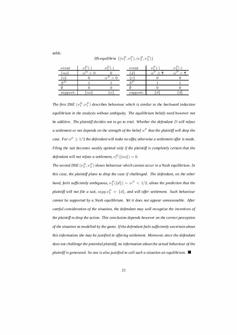
table.DS-equilibria f(ºD

1 ; ºP1 ); (ºD

2 ; ºP2 )g

event ºD1 (¢) ºD

2 (¢)fnog ®D > 0 0fog 0 ®D > 0SD 1 1; 0 0support: fnog fog

event ºP1 (¢) ºP

2 (¢)fdg ®P ¸ 1

2 ®P < 12

fcg 0 0SP 1 1; 0 0support: fdg fdg

The first DSE (ºD1 ;ºP

1 ) describes behaviour which is similar to the backward induction

equilibrium in the analysis without ambiguity. The equilibrium beliefs need however not

be additive. The plaintiff decides not to go to trial. Whether the defendant D will refuse

a settlement or not depends on the strength of the belief ®P that the plaintiff will drop the

case. For ®P ¸ 1=2 the defendant will make no offer, otherwise a settlement offer is made.

Filing the suit becomes weakly optimal only if the plaintiff is completely certain that the

defendant will not refuse a settlement, ºDi (fnog) = 0:

The second DSE (ºD2 ; ºP

2 ) shows behaviour which cannot occur in a Nash equilibrium. In

this case, the plaintiff plans to drop the case if challenged. The defendant, on the other

hand, feels sufficiently ambiguous, ºP2 (fdg) = ®P < 1=2; about the prediction that the

plaintiff will not file a suit, supp ºP2 = fdg; and will offer settlement. Such behaviour

cannot be supported by a Nash equilibrium. Yet it does not appear unreasonable. After

careful consideration of the situation, the defendant may well recognise the incentives of

the plaintiff to drop the action. This conclusion depends however on the correct perception

of the situation as modelled by the game. If the defendant feels sufficiently uncertain about

this information she may be justified in offering settlement. Moreover, since the defendant

does not challenge the potential plaintiff, no information about the actual behaviour of the

plaintiff is generated. So one is also justified to call such a situation an equilibrium.

21

From Part (b) of Definition 3.2 it is clear that no strictly dominated strategy will be

chosen in a DSE. Therefore, one may be led to conclude that all DS-equilibria are backward

induction equilibria. This conclusion is false however, as the DSE (ºD2 ; ºP

2 ) in Example 3.1

demonstrates. Ambiguity may prevent players from choosing strategies which expose them

to situations where they might be hurt by a strictly dominated choice of the opponents. This

may be so, even if they do not expect the opponents to play strictly dominated strategies,

if they do not trust this conclusion sufficiently.

Example 3.1 shows also that the DSE concept can describe behaviour, which is incon-

sistent with the strict consistency requirements of a Nash equilibrium. Indeed, behaviour,

as in equilibrium (ºD2 ; ºP

2 ); can occur only if the worst outcome of an interaction can in-

fluence the decision of a player even if it is on events which are outside the support. If one

would constrain the support notion to make events outside the support Savage-null, i.e.,

irrelevant for the player, then this equilibrium would disappear.

This is obvious from the following lemma which has been proved in Ryan (1998)

(Lemma 1, p.34).

Lemma 3.4 Let º be a capacity on a set S: An event E ½ S is Savage-null if and only if

º(SnE) = 1:

Applying Lemma 3.4 to the equilibrium in Example 3.1 would imply ®D = ®P = 1:

Hence, DSE (ºD2 ; ºP

2 ) would no longer be possible and only the DSE (ºD1 ; ºP

1 ) correspond-

ing to a Nash equilibrium would survive. Indeed, Lo (1996) (Corollary of Proposition 4,

p. 468) shows that this is true for all two-player games. Adopting such a strong notion of

support therefore defeats the objective of modelling ambiguity of players.

22

DSE offers more possibilities to model economic situations than traditional Bayesian

analysis because consistency requirements on beliefs are weaker. In our opinion this ad-

ditional freedom is useful for modelling economic situations since it allows us to include

aspects of the economic environment, which are precluded by Bayesian analysis, but which

are supported by experimental evidence or other robust findings. It is beyond the scope of

this paper to investigate these applications in depth.

3.1.2 Ambiguity and Pessimism

With convex capacities, as we assume throughout this paper, ambiguity aversion is built

into the concept of the Choquet integral. This pessimism concerns however only events

on which there is ambiguity. DSE leaves us with more modelling options. DSE allows us

to distinguish between the preference of players for unambiguous choices and their pes-

simism in the face of ambiguity. For example, if one would like to restrict ambiguity to

an opponent’s strategic behaviour and considers information about types as hard, one can

model this by a capacity which agrees with an additive prior distribution. In this case, pes-

simism is restricted to the behaviour of the opponent but not to the probability over types.

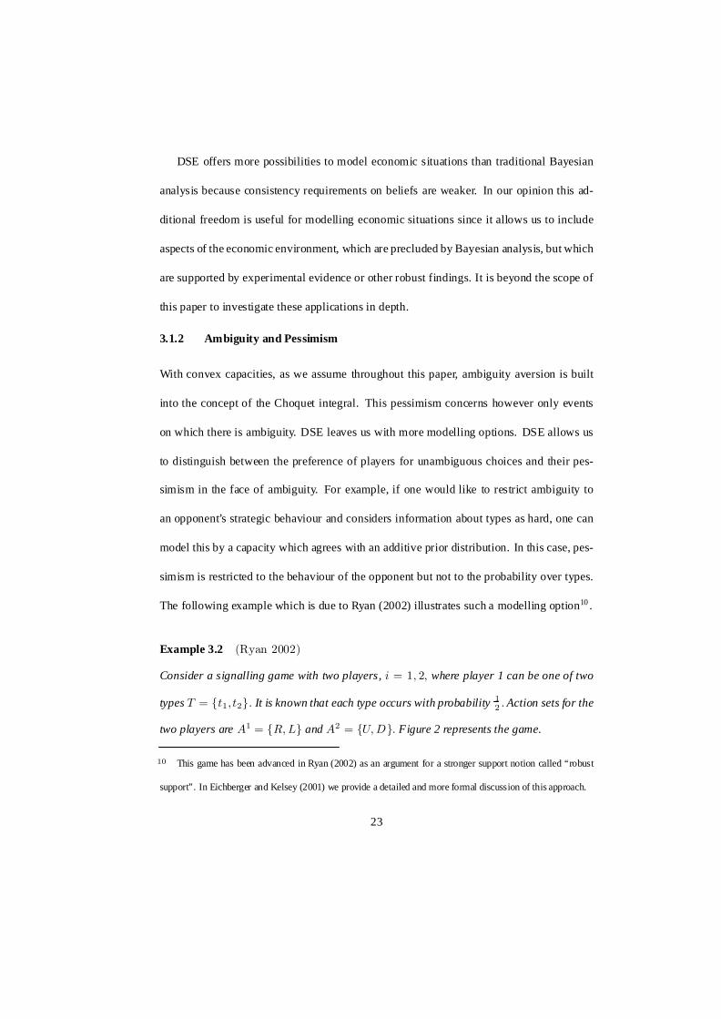
The following example which is due to Ryan (2002) illustrates such a modelling option10 .

Example 3.2 (Ryan 2002)

Consider a signalling game with two players, i = 1; 2; where player 1 can be one of two

types T = ft1; t2g: It is known that each type occurs with probability 12 : Action sets for the

two players are A1 = fR; Lg and A2 = fU; Dg: Figure 2 represents the game.

10 This game has been advanced in Ryan (2002) as an argument for a stronger support notion called ‘‘robust

support’’. In Eichberger and Kelsey (2001) we provide a detailed and more formal discussion of this approach.

23

Insert FIGURE 2 here

It is easy to check that this game has a unique perfect Bayesian equilibrium where

² player 1 of type t1 chooses L;

² player 1 of type t2 chooses R;

² player 2 chooses U in response to L and R:

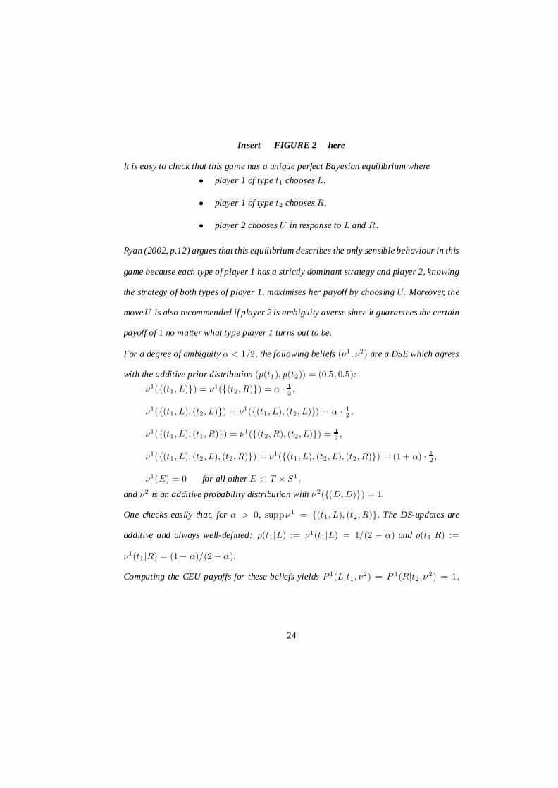
Ryan (2002, p.12) argues that this equilibrium describes the only sensible behaviour in this

game because each type of player 1 has a strictly dominant strategy and player 2, knowing

the strategy of both types of player 1, maximises her payoff by choosing U: Moreover, the

move U is also recommended if player 2 is ambiguity averse since it guarantees the certain

payoff of 1 no matter what type player 1 turns out to be.

For a degree of ambiguity ® < 1=2; the following beliefs (º1; º2) are a DSE which agrees

with the additive prior distribution (p(t1); p(t2)) = (0:5; 0:5):

º1(f(t1; L)g) = º1(f(t2; R)g) = ® ¢ 12 ;

º1(f(t1; L); (t2; L)g) = º1(f(t1; L); (t2; L)g) = ® ¢ 12 ;

º1(f(t1; L); (t1; R)g) = º1(f(t2; R); (t2; L)g) = 12 ;

º1(f(t1; L); (t2; L); (t2; R)g) = º1(f(t1; L); (t2; L); (t2; R)g) = (1 + ®) ¢ 12 ;

º1(E) = 0 for all other E ½ T £ S1;

and º2 is an additive probability distribution with º 2(f(D; D)g) = 1:

One checks easily that, for ® > 0, suppº 1 = f(t1; L); (t2; R)g: The DS-updates are

additive and always well-defined: ½(t1jL) := º1(t1jL) = 1=(2 ¡ ®) and ½(t1jR) :=

º1(t1jR) = (1 ¡ ®)=(2 ¡ ®):

Computing the CEU payoffs for these beliefs yields P 1(Ljt1; º2) = P 1(Rjt2;º 2) = 1;

24

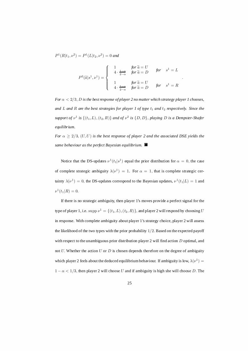
P 1(Rjt1; º2) = P 1(Ljt2; º2) = 0 and

P 2(eajs1; º1) =

8>>>><>>>>:

1 for ea = U4 ¢ 1¡®

2¡® for ea = D for s1 = L

1 for ea = U4 ¢ 1¡®

2¡® for ea = D for s1 = R

:

For ® < 2=3; D is the best response of player 2 no matter which strategy player 1 chooses,

and L and R are the best strategies for player 1 of type t1 and t2 respectively. Since the

support of º1 is f(t1;L); (t2; R)g and of º2 is fD; Dg; playing D is a Dempster-Shafer

equilibrium.

For ® ¸ 2=3; (U; U ) is the best response of player 2 and the associated DSE yields the

same behaviour as the perfect Bayesian equilibrium.

Notice that the DS-updates º 1(t1js1) equal the prior distribution for ® = 0; the case

of complete strategic ambiguity ¸(º1) = 1. For ® = 1; that is complete strategic cer-

tainty ¸(º 1) = 0; the DS-updates correspond to the Bayesian updates, º 1(t1jL) = 1 and

º1(t1jR) = 0:

If there is no strategic ambiguity, then player 1’s moves provide a perfect signal for the

type of player 1, i.e. supp º1 = f(t1; L);(t2; R)g; and player 2 will respond by choosing U

in response. With complete ambiguity about player 1’s strategy choice, player 2 will assess

the likelihood of the two types with the prior probability 1=2: Based on the expected payoff

with respect to the unambiguous prior distribution player 2 will find action D optimal, and

not U: Whether the action U or D is chosen depends therefore on the degree of ambiguity

which player 2 feels about the deduced equilibrium behaviour. If ambiguity is low, ¸(º1) =

1 ¡ ® < 1=3; then player 2 will choose U and if ambiguity is high she will choose D: The

25

critical level which determines when the behaviour of player 2 will change depends, of

course, on the payoff of actions.

If a player feels great ambiguity regarding the strategy of the opponent but not with

respect to the prior type distribution, then DS-updating on the observed actions leads the

player to disregard the ambiguous strategy and to decide based on the unambiguous prior.

Faced with strategic information, a player who is extremely ambiguous about strategic

information and unambiguous about type information will revert to the unambiguous in-

formation of the prior distribution11.

One can, of course, question the assumption about the unambiguous prior distribution.

Indeed, we do not require that beliefs do in general agree with unambiguous priors. It is

an easy exercise to check that, with complete ambiguity about the prior distribution, the

argument that pessimism commends to play U in order to secure the constant payoff of 1

is correct.

3.2 Existence and properties of DSE

Since Bayesian equilibria are DS-equilibria with a degree of ambiguity ¸ = 0, existence of

a DSE is guaranteed under the usual conditions. It is not clear however whether there exist

DS-equilibria for arbitrary degrees of ambiguity ¸ and arbitrary prior beliefs about types.

Proposition 3.5 shows that DS-equilibria exist under the usual assumptions for any degree

of ambiguity.

11 Ryan (2002) considers the case ®= 1=2: In this case, the DSE predicts player 2 to playD:He sees a tension

between the interpretation of Choquet preferences as pessimistic and the preference for the action D which is

risky rather than playing U; an action yielding a constant outcome of 1.

26

Proposition 3.5 For any degree of ambiguity ¸ 2 (0; 1) and any additive prior proba-

bility distribution p on T; there exists a Dempster-Shafer equilibrium with this degree of

ambiguity ¸ which agrees with the distribution p on T:

Proposition 3.5 shows that the DSE concept can be applied in all cases, in which stan-

dard Nash equilibria exist. Moreover, it shows that one can choose the degree of ambiguity

¸ exogenously as a characteristic of a situation and still obtain DS-equilibria. This property

is particularly important in economic applications where one wants to study the impact of

ambiguity on the behaviour of agents12

Games with complete information, i.e., with a type space containing a single type,

jT j = 1; form an important special case to which one can apply DSE. The DSE (ºD2 ; ºP

2 )

in Example 3.1 shows that behaviour in DS-equilibria does not necessarily correspond to

behaviour in backward induction equilibria.

Backward induction in the presence of Knightian uncertainty has also been discussed

by Dow and Werlang (1994). This paper shows that if there is ambiguity, there are non-

backward induction equilibria in the finitely repeated prisoner’s dilemma game. These

equilibria arise with large degrees of ambiguity, which is compatible with our analysis.

Dow and Werlang (1994) analyse games in normal form. Our theory confirms their analysis

with an extensive form solution concept based on Knightian uncertainty. We believe that an

extensive form solution concept is preferable, since DSE requires that equilibrium strategies

are optimal when each move is made. A solution defined on the normal form cannot do

this.

12 Eichberger and Kelsey (2001, 2003) study applications to economic problems.

27

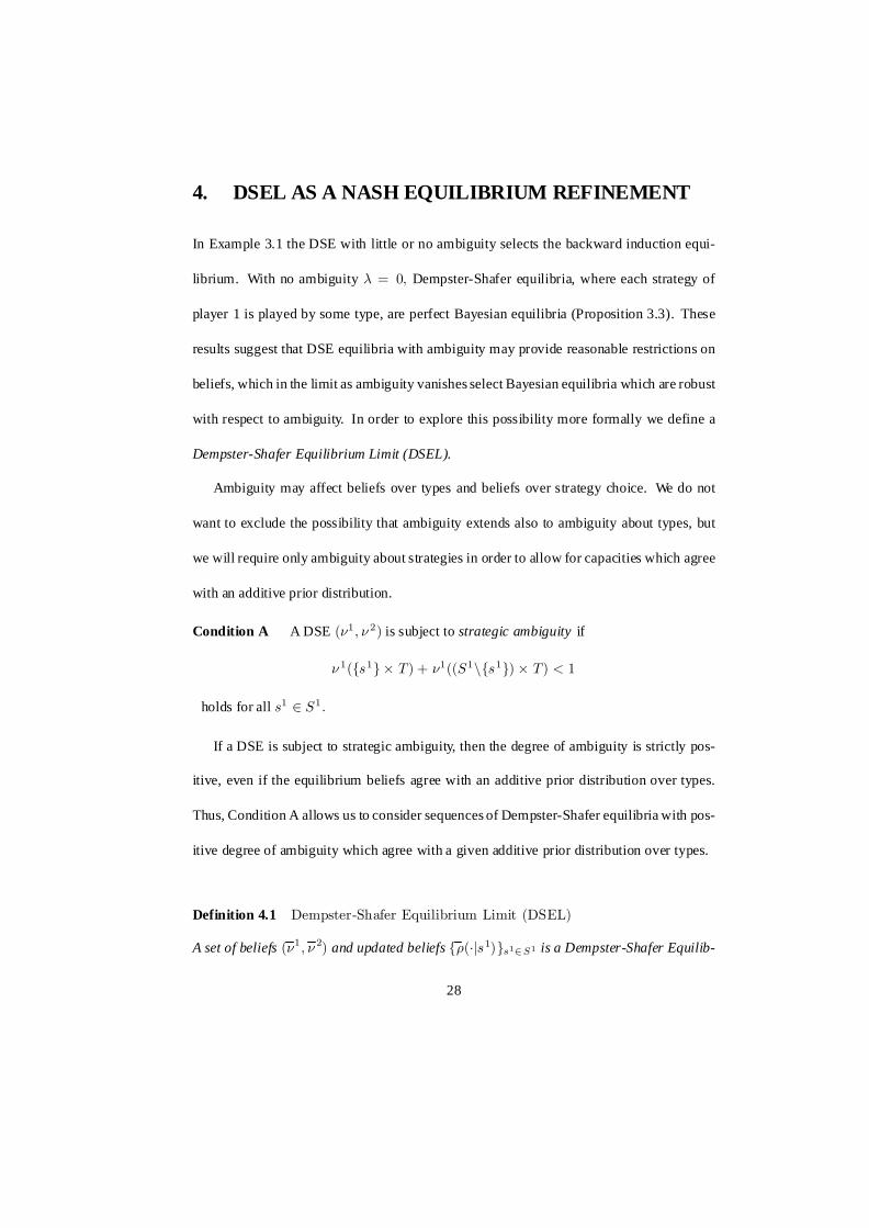
4. DSEL AS A NASH EQUILIBRIUM REFINEMENT

In Example 3.1 the DSE with little or no ambiguity selects the backward induction equi-

librium. With no ambiguity ¸ = 0; Dempster-Shafer equilibria, where each strategy of

player 1 is played by some type, are perfect Bayesian equilibria (Proposition 3.3). These

results suggest that DSE equilibria with ambiguity may provide reasonable restrictions on

beliefs, which in the limit as ambiguity vanishes select Bayesian equilibria which are robust

with respect to ambiguity. In order to explore this possibility more formally we define a

Dempster-Shafer Equilibrium Limit (DSEL).

Ambiguity may affect beliefs over types and beliefs over strategy choice. We do not

want to exclude the possibility that ambiguity extends also to ambiguity about types, but

we will require only ambiguity about strategies in order to allow for capacities which agree

with an additive prior distribution.

Condition A A DSE (º1; º 2) is subject to strategic ambiguity if

º 1(fs1g £ T) + º1((S1nfs1g) £ T) < 1

holds for all s1 2 S1:

If a DSE is subject to strategic ambiguity, then the degree of ambiguity is strictly pos-

itive, even if the equilibrium beliefs agree with an additive prior distribution over types.

Thus, Condition A allows us to consider sequences of Dempster-Shafer equilibria with pos-

itive degree of ambiguity which agree with a given additive prior distribution over types.

Definition 4.1 Dempster-Shafer Equilibrium Limit (DSEL)

A set of beliefs (º1; º 2) and updated beliefs f½(¢js1)gs12S1 is a Dempster-Shafer Equilib-

28

rium Limit (DSEL) if it is the limit of a sequence of strategically ambiguous Dempster-

Shafer equilibria ((º1n; º 2

n);

f½n(¢js1)gs12S1) such that the degree of ambiguity ¸ tends to zero as n tends to infinity.

By Proposition 3.5 there exists a DSE¡(º1

n; º 2n); f½n(¢js1)gs12S1

¢for any degree of

ambiguity ¸n > 0; where, for all s1 2 S1; ½n(¢js1) is well-defined by the DS-updates

º1n(¢js1): By convexity of the capacities, º i

n(E) 2 [0; 1]; for all events E µ Si ; i = 1; 2;

and for all n: Since we consider finite games, the sequence (º1n ; º2

n) is contained in [0; 1]m;

where m = jT j+ jS1j +jS2j: Hence, for any sequence ¸n ! 0 there must be a converging

subsequence (º 1n; º2

n ) ! (º 1;º 2) and ½n(¢js1) ! ½(¢js1) for all s1 2 S1: Thus, DSEL is

always well-defined.

Notice that a DSEL requires also to specifya sequence of updated capacities f½n(¢js1)gs12S1 :

Since we impose strategic ambiguity there exists always a supporting sequence of Dempster-

Shafer equilibria for which the updated beliefs f½n(¢js1)gs12S1 are well defined by the

DS-updates. Even if DS-updates are well-defined along the sequence of DS-equilibria, a

DSEL¡(º1; º 2); f½(¢js1)gs12S1

¢may have non-additive DS-updates ½(¢js1) for strategies

s1; which are not played in equilibrium.

The following example shows that beliefs off the equilibrium path need not be additive.

In particular, the sequence of DS-equilibria supporting a DSEL

² can be strategically ambiguous,

² agree with an additive prior distribution and

² have well-defined DS-updates.

29

Notice that a DSEL also requires the specification of a sequence of updated capacities.

Yet, as the degree of ambiguity converges to zero, additive beliefs (º 1;º 2) obtain in the

limit, but DS-updates ½(¢js1) may remain non-additive if strategy s1 is not played in the

DS-equilibria of the supporting sequence.

Example 4.1 Consider the signalling game, in Figure 3.

Insert FIGURE 3 here

The strategy set of player 1 is A1 = fL; Rg and of player 2, A2 = fu; m; dg: There are

two types of player 1, T = ft1; t2g, which occur with probability p1 and p2; p1 > p2 for

concreteness.

In any perfect Bayesian equilibrium both types of player 1 choose R; since any belief ¹(¢jR)

makes d strictly dominated for player 2. But if player 2 plays d with probability zero,

strategy R strictly dominates strategy L for player 1. Hence, there is a unique perfect

Bayesian equilibrium where player 2 chooses u:

There are two types of DSEL agreeing with the additive prior distribution (p1;p2): The

completely additive DSEL³(eº1; eº 2); (e½(¢jR);e½(¢jL))

´; eº1(t1; R) = p1; eº 1(t2;R) = p2;

e½(t1jR) = p1; e½(t2jR) = p2; eº 2(u) = 1; is behaviourally equivalent to the perfect

Bayesian equilibrium. This DSEL is supported by a sequences of strategically ambiguous

E-capacities which agree with the prior distribution. For details about the construction of

such a sequence see Eichberger and Kelsey (1999).

There is however another DSEL (º1; º 2) where the updated beliefs of player 1 are not

30

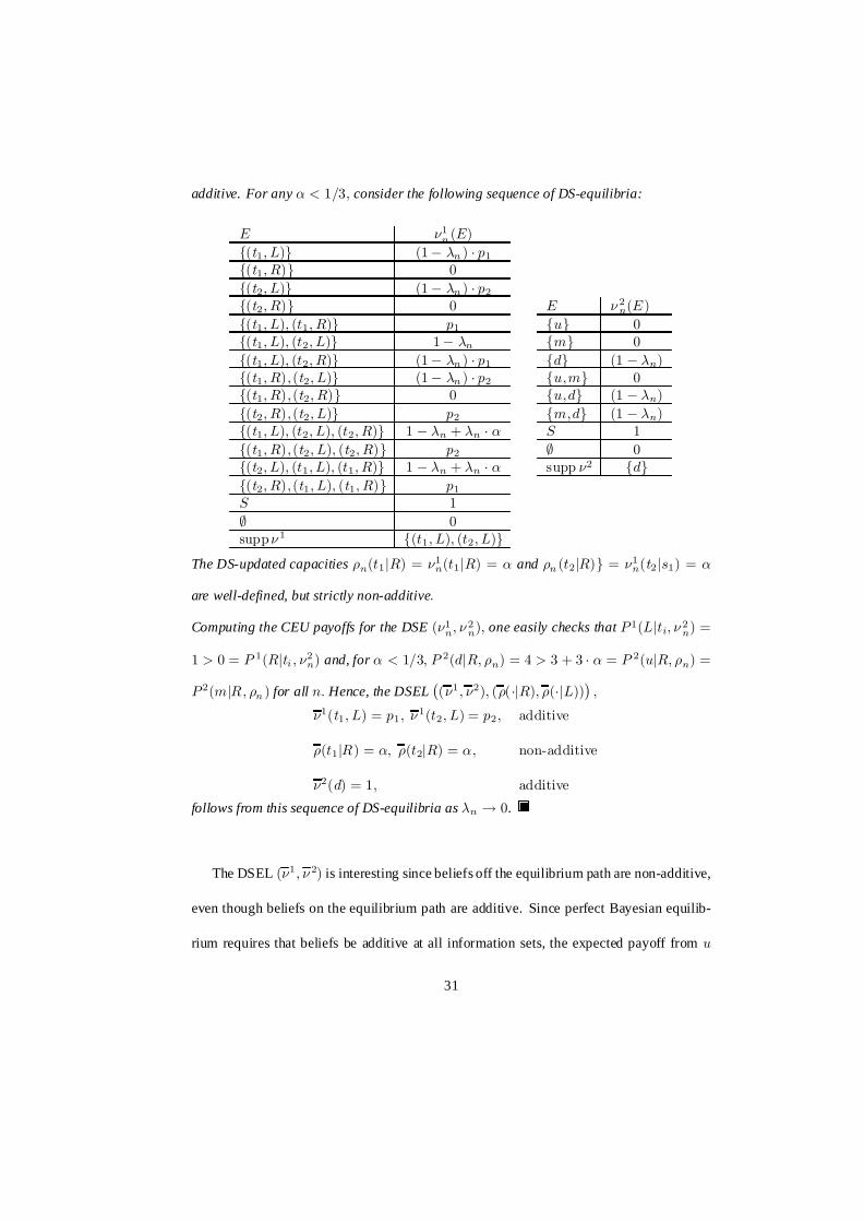
additive. For any ® < 1=3; consider the following sequence of DS-equilibria:

E º1n (E)

f(t1; L)g (1 ¡ ¸n ) ¢ p1f(t1; R)g 0f(t2; L)g (1 ¡ ¸n ) ¢ p2f(t2; R)g 0f(t1; L); (t1; R)g p1f(t1; L); (t2; L)g 1 ¡ ¸n

f(t1; L); (t2; R)g (1 ¡ ¸n ) ¢ p1f(t1; R);(t2; L)g (1 ¡ ¸n ) ¢ p2f(t1; R);(t2; R)g 0f(t2; R);(t2; L)g p2f(t1; L); (t2; L); (t2; R)g 1 ¡ ¸n + ¸n ¢ ®f(t1; R);(t2; L); (t2; R)g p2f(t2; L); (t1; L); (t1; R)g 1 ¡ ¸n + ¸n ¢ ®f(t2; R);(t1; L); (t1; R)g p1S 1; 0suppº 1 f(t1; L); (t2; L)g

E º 2n(E)

fug 0fmg 0fdg (1 ¡ ¸n)fu;mg 0fu;dg (1 ¡ ¸n)fm;dg (1 ¡ ¸n)S 1; 0supp º2 fdg

The DS-updated capacities ½n(t1jR) = º1n(t1jR) = ® and ½n (t2jR)g = º1

n(t2js1) = ®

are well-defined, but strictly non-additive:

Computing the CEU payoffs for the DSE (º1n; º 2

n); one easily checks that P 1(Ljti; º 2n) =

1 > 0 = P 1(Rjti ; º2n) and, for ® < 1=3; P 2(djR; ½n) = 4 > 3 + 3 ¢ ® = P 2(ujR; ½n) =

P 2(mjR; ½n ) for all n: Hence, the DSEL¡(º1; º2); (½(¢jR); ½(¢jL))

¢;

º1(t1; L) = p1; º 1(t2; L) = p2; additive

½(t1jR) = ®; ½(t2jR) = ®; non-additive

º2(d) = 1; additive

follows from this sequence of DS-equilibria as ¸n ! 0.

The DSEL (º1; º 2) is interesting since beliefs off the equilibrium path are non-additive,

even though beliefs on the equilibrium path are additive. Since perfect Bayesian equilib-

rium requires that beliefs be additive at all information sets, the expected payoff from u

31

dominates the payoff from d. DSEL, however, allows strict non-additivity off the equilib-

rium path, so that the certain payoff of 4 obtained from strategy d becomes more attractive.

It is plausible that a player who has observed an out-of-equilibrium move will have some

doubts about his original theory of how the game is played. This could cause him to be-

come ambiguity-averse as represented by the non-additivity of the updated beliefs. DSEL

allows us to model ambiguity of a player as a consequence of having to update beliefs on

events with a capacity weight of zero.

Example 4.1 shows also that there are few constraints on the DS-updates. Indeed, DSE,

and therefore DSEL, allow us to impose constraints on players’ beliefs directly and to de-

duce equilibrium beliefs satisfying these constraints. This opens the opportunity to de-

sign experiments where ambiguity is manipulated independently from the equilibrium play

which one wants to test.

4.1 Properties of DSEL

In this section, we will compare the concept of a DSEL with Bayesian and perfect Bayesian

equilibrium. Since Bayesian and perfect Bayesian equilibria have an additive prior dis-

tribution over types as a defining criterion we will restrict attention to Dempster-Shafer

equilibria which agree with an additive prior distribution throughout this section.

The capacities (º1; º2) of a DSEL are additive. So it is not difficult to prove that a

DSEL is a Bayesian equilibrium.

Proposition 4.2 A DSEL which agrees with an additive prior distribution over types is a

Bayesian equilibrium.

32

All DSEL are Bayesian equilibria. The potential of strategic ambiguity to select among

the set of Bayesian equilibrium lies in the updated beliefs. Beliefs are generated by the DS-

updating rule in combination with constraining assumptions about equilibrium beliefs. A

DSE does not tie down the equilibrium beliefs as much as Nash equilibrium does. Hence,

there is room for game-specific constraints on beliefs and attitudes towards ambiguity. De-

pending on the application one can focus on the consequences of the degree of ambiguity

aversion, of ambiguity about types or of other characteristics of beliefs. The DS-updates

inherit their properties from these fundamental assumptions. To the extent that one can

control for the degree of ambiguity, ambiguity aversion and other characteristics of an en-

vironment one may be able to test equilibrium properties in experiments.

One of the weakest refinements of Bayesian equilibria is a perfect Bayesian equilib-

rium. By making updated beliefs part of the equilibrium concept it guarantees optimising

behaviour at all information sets whether or not they will be reached in equilibrium. Since

perfect Bayesian equilibrium puts no constraint on out-of-equilibrium beliefs, it eliminates

only equilibria relying on strictly dominated strategies at information sets off the equilib-

rium path.

A DSEL allows for beliefs off the equilibrium path which are strictly non-additive.

Hence, Example 4.1 shows that a DSEL need not be a perfect Bayesian equilibrium. One

may however conjecture that a DSEL with additive updates f½(¢js1)gs12S1 at all informa-

tion sets is a perfect Bayesian equilibrium. We will show below in Proposition 4.3 that this

is the case, indeed.

One may also conjecture that the restrictions on beliefs induced by the sequence of state-

33

gically ambiguous Dempster-Shafer equilibria would rule out DSEL with additive updates

f½(¢js1)gs12S1 at all information sets where a player uses a weakly dominated action. This

is however not true. For every perfect Bayesian equilibrium it is possible to construct a

sequence of strategically ambiguous DS-equilibria, which agree on the additive prior over

types and converges to this perfect Bayesian equilibrium. This is almost obvious if all in-

formation sets will be reached in the perfect Bayesian equilibrium. If there are information

sets following actions which are not played in a perfect Bayesian equilibrium, then one

can find a sequence of DS-equilibria in which the DS-updates are not defined at these in-

formation sets. Hence, one can assign the off-the-equilibrium-path beliefs of the perfect

Bayesian equilibrium to those DS-equilibria. Thus, one can obtain even a perfect Bayesian

equilibrium where player 2 chooses weakly dominated strategies off the equilibrium path

as a DSEL.

Proposition 4.3 Perfect Bayesian equilibrium and DSEL

(i) Every perfect Baysian equilibrium is a DSEL.

(ii) A DSEL which agrees with an additive prior distribution is a perfect Bayesian equi-

librium if all updates are additive.

DS-updates of a DSEL can, but need not, be additive. Proposition 4.3 shows that ad-

ditive limits of the DS-updates is the crucial condition for the two concepts to coincide. If

DS-updates do not converge to additive probability distributions off the equilibrium path,

then strategic ambiguity, modelled by the DS equilibrium concept, provides a refinement

of Nash equilibrium based on other principles than standard refinements in the literature.

Mailath (1992) provides an excellent survey of the refinements most commonly used in

34

signalling games. They all operate by restricting out-of-equilibrium beliefs. Justification

for such restrictions is obtained by forward or backward induction arguments. There is an

obvious tension in such arguments because out-of-equilibrium behaviour is constrained by

reasoning about behaviour which will never be observed.

The DSEL provides an alternative approach to equilibrium selection. Modelling am-

biguity about the equilibrium strategy choices directly avoids the tension in the interpre-

tation of out-of-equilibrium beliefs. Moreover, there are behavioural theories behind the

DS-updating rule (Gilboa and Schmeidler, 1993) and the Choquet expected utility model

(Gilboa, 1987; Sarin and Wakker, 1993). Assumptions about the behavioural foundations

of this decision and updating model can and have been tested independently from the equi-

librium notion (Camerer and Weber, 1992).

4.2 Out-of-equilibrium beliefs

Refinement of the set of equilibria can be obtained by imposing additional restrictions

on the players’ non-additive beliefs. As in the standard refinement literature, one can

strengthen or weaken the robustness requirement imposed on Bayesian equilibrium by

putting further constraints on the sequence of ambiguous DS-equilibria which support it.

In contrast to this literature such assumptions are in principle testable.

DS-equilibria which are not perfect Bayesian equilibria are plausible, since they corre-

spond to cases in which player 2 is ambiguity-averse after observing an unexpected move.

Example 4.1 illustrates the potential of DSEL to select among Bayesian equilibria based

on ambiguity about the behaviour in case of an unexpected out-of-equilibrium move. Yet,

even if we do not want to rely on non-additive beliefs off the equilibrium path, DSEL offers

35

quite intuitive out-of-equilibrium beliefs.

It is impossible to develop here a complete theory of reasonable refinements based on

ambiguity, but the following example may provide some intuition. It is a simplified version

of the education-signalling model introduced by Spence (1973). With plausible restrictions

on the out-of-equilibrium beliefs ambiguity may select the pooling equilibrium as the a

unique DSEL13. The intuition about beliefs is as follows. A DS-equilibrium which agrees

with an additive prior distribution over types models a situation where a player feels ambi-

guity about the opponents’ behaviour but not about the prior distribution over types. This

is a natural assumption if past experience has provided information about the frequency of

types but if there is no well-established way of signalling private information. In such a

situation signalling is endogenous equilibrium behaviour. An out-of-equilibrium move in-

dicates a break-down of the implicit understanding of equilibrium behaviour. In such a case,

it appears quite reasonable to return to the ‘‘firm’’ information about the prior distribution

over types.

Example 4.2 education signalling14

Consider two workers with different productivity, ÁH > ÁL: A worker’s productivity is

private information but it is common knowledge that the proportion of high-productivity

workers is p: Workers will apply for a position in the firm with a wage proposal. A worker

13 Notice that Example 4.2 is no contradiction to the result in Proposition 4.3. There are other DSELs corre-

sponding to the typical perfect Bayesian equilibria of the Spence signalling model.14 This is a highly stylised version of the education signalling model by Spence (1973). For simplicity of the

exposition, we have assumed that the education level is not a choice variable. A more general treatment of the

education signalling model can be found in Eichberger and Kelsey (1999a).

36

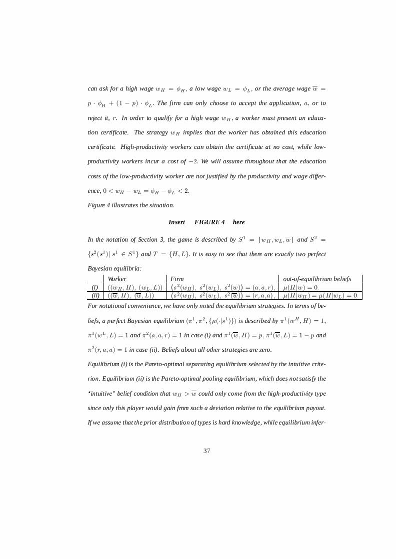
can ask for a high wage wH = ÁH ; a low wage wL = ÁL; or the average wage w =

p ¢ ÁH + (1 ¡ p) ¢ ÁL: The firm can only choose to accept the application, a; or to

reject it, r. In order to qualify for a high wage wH ; a worker must present an educa-

tion certificate. The strategy wH implies that the worker has obtained this education

certificate. High-productivity workers can obtain the certificate at no cost, while low-

productivity workers incur a cost of ¡2: We will assume throughout that the education

costs of the low-productivity worker are not justified by the productivity and wage differ-

ence, 0 < wH ¡ wL = ÁH ¡ ÁL < 2.

Figure 4 illustrates the situation.

Insert FIGURE 4 here

In the notation of Section 3, the game is described by S1 = fwH ; wL; wg and S2 =

fs2(s1)j s1 2 S1g and T = fH; Lg: It is easy to see that there are exactly two perfect

Bayesian equilibria:

Worker Firm out-of-equilibrium beliefs(i) ((wH ; H); (wL; L))

¡s2(wH ); s2(wL); s2(w)

¢= (a; a; r); ¹(H jw) = 0:

(ii) ((w; H); (w; L))¡s2(wH ); s2(wL); s2(w)

¢= (r; a;a); ¹(H jwH ) = ¹(H jwL) = 0:

For notational convenience, we have only noted the equilibrium strategies. In terms of be-

liefs, a perfect Bayesian equilibrium (¼1; ¼2; f¹(¢js1)g) is described by ¼1(wH ; H) = 1;

¼1(wL; L) = 1 and ¼2(a; a; r) = 1 in case (i) and ¼1(w; H) = p; ¼1(w; L) = 1 ¡ p and

¼2(r; a; a) = 1 in case (ii). Beliefs about all other strategies are zero.

Equilibrium (i) is the Pareto-optimal separating equilibrium selected by the intuitive crite-

rion. Equilibrium (ii) is the Pareto-optimal pooling equilibrium, which does not satisfy the

‘‘intuitive’’ belief condition that wH > w could only come from the high-productivity type

since only this player would gain from such a deviation relative to the equilibrium payout.

If we assume that the prior distribution of types is hard knowledge, while equilibrium infer-

37

ences about behaviour are ambiguous, then only behaviour of the pooling equilibrium (ii)

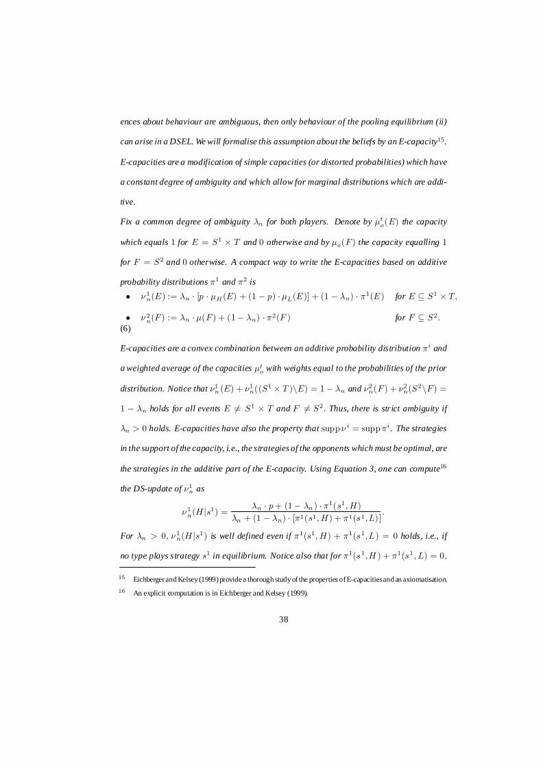
can arise in a DSEL. We will formalise this assumption about the beliefs by an E-capacity15.

E-capacities are a modification of simple capacities (or distorted probabilities) which have

a constant degree of ambiguity and which allow for marginal distributions which are addi-

tive.

Fix a common degree of ambiguity ¸n for both players. Denote by ¹to(E) the capacity

which equals 1 for E = S1 £ T and 0 otherwise and by ¹o(F ) the capacity equalling 1

for F = S2 and 0 otherwise. A compact way to write the E-capacities based on additive

probability distributions ¼1 and ¼2 is

² º 1n(E) := ¸n ¢ [p ¢ ¹H (E) + (1 ¡ p) ¢ ¹L(E)] + (1 ¡ ¸n) ¢ ¼1(E) for E µ S1 £ T;

² º 2n(F ) := ¸n ¢ ¹(F ) + (1 ¡ ¸n) ¢ ¼2(F ) for F µ S2:

(6)

E-capacities are a convex combination between an additive probability distribution ¼i and

a weighted average of the capacities ¹to with weights equal to the probabilities of the prior

distribution. Notice that º1n (E) + º1

n((S1 £ T )nE) = 1 ¡ ¸n and º2n(F ) + º2

n(S2nF ) =

1 ¡ ¸n holds for all events E 6= S1 £ T and F 6= S2: Thus, there is strict ambiguity if

¸n > 0 holds. E-capacities have also the property that suppº i = supp¼i . The strategies

in the support of the capacity, i.e., the strategies of the opponents which must be optimal, are

the strategies in the additive part of the E-capacity. Using Equation 3, one can compute16

the DS-update of º1n as

º 1n(H js1) =

¸n ¢ p + (1 ¡ ¸n ) ¢ ¼1(s1; H)¸n + (1 ¡ ¸n) ¢ [¼1(s1; H) + ¼1(s1;L)]

:

For ¸n > 0; º 1n(H js1) is well defined even if ¼1(s1; H) + ¼1(s1;L) = 0 holds, i.e., if

no type plays strategy s1 in equilibrium. Notice also that for ¼1(s1;H ) + ¼1(s1; L) = 0;

15 Eichbergerand Kelsey (1999)providea thorough study of the properties ofE-capacitiesand an axiomatisation.16 An explicit computation is in Eichberger and Kelsey (1999).

38

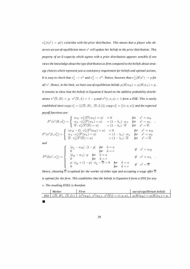
º1n(tjs1) = p(t) coincides with the prior distribution. This means that a player who ob-

serves an out-of-equilibrium move s1 will update her beliefs to the prior distribution. This

property of an E-capacity which agrees with a prior distribution appears sensible if one

views the knowledge about the type distribution as firm compared to the beliefs about strat-

egy choices which represent just a consistency requirement for beliefs and optimal actions.

It is easy to check that º1n ! ¼1 and º 2

n ! ¼2: Notice, however, that º 1n(H js1) ! p for

all s1: Hence, in the limit, we have out-of-equilibrium beliefs ¹(H jwH ) = ¹(H jwL) = p.

It remains to show that the beliefs in Equation 6 based on the additive probability distrib-

utions ¼1(w; H) = p; ¼1(w; L) = 1 ¡ p and ¼2(r; a; a) = 1 form a DSE. This is easily

established since supp º1n = f((w; H); (w;L))g; supp º2

n = f(r; a; a)g and the expected

payoff functions are:

P 1(s1jH; º2n ) =

8<:

wH ¢ º 1n(s2(wH ) = a) = 0 for s1 = wH

wL ¢ º 1n(s2(wL) = a) = (1 ¡ ¸n) ¢ wL for s1 = wL

w ¢ º1n(s2(w) = a) = (1 ¡ ¸n) ¢ w for s1 = w

;

P 1(s1jL; º2n ) =

8<:

(wH ¡ 2) ¢ º1n(s2(wH ) = a) = 0 for s1 = wH

wL ¢ º 1n(s2(wL) = a) = (1 ¡ ¸n) ¢ wL for s1 = wL

w ¢ º1n(s2(w) = a) = (1 ¡ ¸n) ¢ w for s1 = w

and

P 2(eajs1; º 1n) =

8>>>>>><>>>>>>:

[ÁL ¡ wH ] ¢ [1 ¡ p] for ea = a0 for ea = r if s1 = wH

[ÁH ¡ wL] ¢ p for ea = a0 for ea = r if s1 = wL

p ¢ ÁH + (1 ¡ p) ¢ ÁL ¡ w = 0 for ea = a0 for ea = r if s1 = w

:

Hence, choosing w is optimal for the worker of either type and accepting a wage offer w

is optimal for the firm. This establishes that the beliefs in Equation 6 form a DSE for any

n: The resulting DSEL is therefore

Worker Firm out-of-equilibrium beliefs(iii) ((w; H); (w; L))

¡s2(wH ); s2(wL); s2(w)

¢= (r; a; a); ¹(H jwH ) = ¹(H jwL) = p:

39

The equilibrium selection in the DSEL of Example 4.2 depends on the joint assump-

tions of an unambiguous prior distribution over types and a degree of ambiguity aversion

¸n which, for each step n; is the same for all events E ½ S1 £ T: Constant ambiguity

aversion controls for distorted beliefs17. The result that out-of-equilibrium beliefs coincide

with the additive prior distribution is driven by the assumption that the prior distribution is

unambiguously known. If this is the case, it makes sense for a player to revert to the un-

ambiguous information as implied by DS-updating, whenever an out-of-equilibrium move

occurs which invalidates the equilibrium behaviour prediction. In the game of Example

4.2, this assumption about the prior distribution rules out the separating equilibrium. The

separating equilibrium would require complete trust in the equilibrium behaviour because

a low-productivity worker has an incentive to break away from the separating equilibrium

and to propose the average wage rather than the low wage. To argue that the firm should

assume that an average wage offer could only come from the low-productivity type would

mean that the firm feels no ambiguity about the behaviour of the workers.

In contrast to Bayesian equilibrium, DSE has a updating rule which works also for

out-of-equilibrium beliefs if there is some ambiguity about strategy choices. Reasonable

assumptions about beliefs can be imposed directly. For example, partial information can be

assumed as in the case of a well-known prior distribution in Example 4.2. Whether this is

an appropriate assumption or not can be assessed independent from the equilibrium, which

is an advantage in economic applications.

17 To establish the result of Proposition 4.3 that every perfect Bayesian equilibrium is a DSEL we had to relax

this assumption of a constant degree of ambiguity in each step of the belief sequence supporting the DSEL.

40

5. CONCLUSION

We have applied the theory of Knightian uncertainty to sequential games. The evidence

suggests that there are occasions in which individuals have large degrees of ambiguity.

Despite this we believe that an interesting case is when the degree of ambiguity is small.

Under this assumption, we have shown that our definition of equilibrium is a refinement of

Bayesian equilibrium, which is similar in spirit to perfect Bayesian equilibrium but does not

exactly coincide with it. Since DSEL is a special case of Bayesian equilibrium, no irrational

behaviour is introduced by considering non-additive beliefs. As we have shown, even in

the limit as beliefs converge to additive probabilities, significant deviations from behaviour

under subjective expected utility are possible off the equilibrium path. We believe this is

one of our main innovations.

41

Appendix

PROOFS

Lemma 2.2: If a convex capacity º has zero degree of ambiguity then it is additive.

Proof. Suppose that º is not additive, then there exist A; B ½ S , such that A \ B = ; and

º(A [ B) > º(A) + º (B): Let C = Sn(A [ B). Then since the degree of ambiguity is

zero:

1 = º(A [ B) + º (C) > º (A) + º(B) + º(C ):(A-1)

By convexity, 1 = º((A[B)[(A[C )) > º(A[B)+º(A[C )¡º(A): Since the degree

of ambiguity is zero, º(A [ B) = 1 ¡ º (C) and º(A [ C) = 1 ¡ º(B): Substituting, we

obtain 1 > 1 ¡ º (C) + 1 ¡ º(B) ¡ º (A); but this contradicts A-1.

Proposition 3.3:

a) A Dempster-Shafer Equilibrium (º 1; º2) with a degree of ambiguity ¸ = 0; for

which the belief of player 2, º1; agrees with the additive prior distribution p on T is

a Bayesian Equilibrium.

b) Consider a Dempster-Shafer Equilibrium (º 1; º2) with a degree of ambiguity

¸ = 0; for which the belief of player 2, º1; agrees with the additive prior distribution p

on T: If for each strategy s1 2 S1 there exists a type t 2 T such that (s1; t) 2 suppº ;

then the Dempster-Shafer Equilibrium (º1; º2) is a perfect Bayesian equilibrium.

Proof. Part (a): Since the DSE (¼1; ¼2) has a degree of ambiguity ¸ = 0, by Lemma 2.2,

¼1 and ¼2 must be additive probability distributions. Since the DSE agrees with an additive

42

prior distribution p on T;P

s12S1 ¼1(s1; t) = p(t) for all t 2 T: Hence, condition DSE-a

of Definition 3.2 can be written as

s1 2arg maxes12S1

X

s22S2

¼2(s2) ¢ u1(es1; s2(s1); t)

for all s1 2 S1 with ¼1(s1; t) > 0 and all t 2 T: Condition DSE-b requires

s2(s1) 2arg maxea2A2

X

t2T

½(tjs1) ¢ u2(s1; ea; t)

for all s2 2 S2 with ¼2(s2) > 0: By Condition DSE-c and Equation 3,

½(tjs1) := ¼1(S1 £ ftgjfs1g £ T) = ¼1(s1; t)Pt2T ¼1(s1; t)

providedP

t2T ¼1(s1; t) 6= 0: Note that beliefs off the equilibrium path ½(tjs1) are arbi-

trary and need not even be additive. For actions s1 2 S1 such thatP

t2T ¼1(s1; t) = 0 all

actions a 2 A2 are optimal. Hence, Part (a) of Proposition 3.3 defines a Bayesian equilib-

rium with mixed strategies (¼1; ¼2):

Part (b): If, in addition, for each strategy s1 2 S1 there exists a type t 2 T such that

(s1; t) 2 supp ¼1; thenP

t2T ¼1(s1; t) 6= 0 for alls1 2 S1 and ½(tjs1) = (¼1(s1; t))=(P

t2T ¼1(s1; t))

is defined at all information sets. In this case, (¼1; ¼2) is a perfect Bayesian equilibrium.

Lemma 3.4: Let º be a capacity on a set S: An event E ½ S is Savage-null if and only if

º(SnE) = 1:

Proof. An event E is Savage-null if for any three outcomes x; y;z 2 X the CEU value of

the acts xEy and zEy are equal, i.e.

u(x) ¢ º(E) + u(y) ¢ [1 ¡ º(E)] = u(y) ¢ º(SnE) + u(z) ¢ [1 ¡ º(SnE)]

where we assume, without loss of generality, u(x) > u(y) > u(z): This equality can hold

for arbitrary outcomes x; y; z 2 X with this order if and only if º(SnE) = 1 and º (E) = 0:

43

Proposition 3.5: For any degree of ambiguity ¸ 2 (0; 1) and any additive prior proba-

bility distribution p on T; there exists a Dempster-Shafer equilibrium with this degree of

ambiguity ¸; which agrees with the distribution p on T:

Proof. The proof uses the special form of an E-capacity, which is extensively discussed

in Eichberger and Kelsey (1999). E-capacities are modifications of an additive probability

distribution with a constant degree of ambiguity and, possibly, some additive marginal dis-

tributions. If there are no additive marginals then E-capacities are simple capacities. More-

over, the support of an E-capacity coincides with the support of its additive part. Hence,

for given prior distributions of types and given degrees of ambiguity, E-capacities are com-

pletely described by their additive part. Given beliefs modelled by E-capacities, one can

use standard arguments to show that there is a Nash-equilibrium in mixed strategies for the

modified game where the Choquet payoff functions are viewed as functions of the additive

part of the E-capacities.

Fix ¸1; ¸2 2 (0;1) and any additive probability distribution p on T: For any finite set X

denote by ¢(X) the set of additive probability distributions on X: Let ¢p(S1 £ T) be the

set of additive probability distributions on S1 £ T with marginal distribution p on T: This

set is non-empty, compact and convex.

For any E ½ S1 £ T let the capacity ºt be defined as

ºt(E) :=½

1 if S1 £ ftg ½ E0 otherwise

;

44

and for any ¼ 2 ¢p(S1 £ T ) consider the capacity

º 1¼(E) := ¸1¢

X

t2T

p(t) ¢ ºt(E) + (1 ¡ ¸1) ¢ ¼(E):(A-2)

For any set T 0 ½ T; the DS-update of the capacity defined in Equation A-2 is (see Eich-

berger and Kelsey, 1999, Lemma 4.2, p. 132)

º1¼(T 0js1) =

¸1¢ Pt2T 0

p(t) + (1 ¡ ¸1)¢ Pt2T 0

¼(s1; t)

Pt2T

¼(s1; t) + ¸1 ¢·1¡ P

t2T¼(s1; t)

¸ :(A-3)

For ¸1 > 0, º1¼ (T 0js1) is a continuous function of ¼:

For any s1 2 S1 and any ¼ 2 ¢p (S1 £ T); let

½(¼; s1) =arg max¾2¢(A2 )

X

a2A2

¾(a) ¢ P 2(ajs1; º1¼)(A-4)

be the set of best behaviour strategies on A2 for given history s1 and given belief º1¼ based

on ¼:

From the definition of the Choquet integral in Equation 1, it is clear that P 2(ajs1; º1¼)

is a continuous function of the capacity º1¼: From the DS-update in Equation A-3 we

know that º 1¼ is a continuous function of ¼: Thus,

Pa2A2

¾(a) ¢ P 2(ajs1; º1¼) is a continu-

ous function of ¼: Hence, by Berge’s maximum theorem (e.g., Takayama, 1985, p. 254),

½(¼; s1) is a upper-hemi-continuous correspondence. Since ¢(A2) is a convex set and

sinceP

a2A2¾ (a) ¢ P 2(ajs1; º1

¼ ) is linear in ¾; the correspondence ½(¼; s1) is also convex-

valued.

For any t 2 T and a vector ¹ = (¹(¢js1))s12S1 of additive probability distributions

¹(¢js1) 2 ¢(A2) define the capacities º 2¹(E js1) := (1 ¡ ¸2) ¢ ¹(E js1): The capacity

º2¹(¢js1) is continuous in ¹: Let

Ã(¹; t) =arg max¾2¢(S1)

X

s12S1

¾(s1) ¢ P 1(s1jt; º 2¹(¢js1))(A-5)

45

be the best-response correspondence for player 1. Finally, let

Á(¹) := f¼ 2 ¢p(S1 £ T)j ¼(s1; t) =X

t2T

p(t) ¢ ¾t(s1); ¾t 2 Ã(¹; t)g:(A-6)

Since the Choquet integral P 1(s1jt;º 2¹(¢js1)) is continuous in º2

¹ (¢js1); which in turn

is continuous in ¹; we can conclude thatP

s12S1¾(s1) ¢ P 1(s1jt; º2

¹(¢js1)) is continuous

in ¹: Moreover, the objective function is linear in ¾: Applying Berge’s maximum theo-

rem again, we conclude that the correspondences Ã(¹; t) are upper-hemi-continuous and

convex-valued. The correspondence Á(¹) defined in Equation A-6 is a convex set for each

¹ and clearly also upper-hemi-continuous.

Consider the mapping £ : ¢p(S1 £ T ) £ ¢(A2)jS1j ! ¢p(S1 £ T ) £ ¢(A2)jS1 j

defined by

(¼; ¹) 7! £(¼; ¹) := £s12S1

½(¼; s1) £ Á(¹):

As the Cartesian product of upper-hemi-continuous and convex-valued correspondences

£ is itself a upper-hemi-continuous and convex-valued correspondence. Moreover, the set

¢p(S1 £ T) £ ¢(A2)jS1j is compact and convex. Hence one can apply Kakutani’s fixed-

point theorem to establish the existence of (¼¤; ¹¤) 2 £(¼¤; ¹¤):

Define the additive probability distribution ¿¤ on S2; the set of strategies of player 2, by

¿¤(s2) :=Q

s12S1¹¤(s2(s1)js1) for all s2 2 S2: For all E ½ S2; let º 2

¿¤(E) := (1 ¡ ¸2) ¢

¿¤(E):

We claim that the capacities (º1¼¤ ; º2

¿¤) are a DSE. To see this, note first that suppº 1¼¤ =

fs1 2 S1j ¼¤(s1) > 0g and supp º2¿¤ = fs2 2 S2j ¿ ¤(s2) > 0g (Eichberger and Kelsey,

1999, Lemma 2.2, p. 121). Hence, (s1; t) 2 suppº 1¼¤ implies ¼¤(s1; t) = p(t)¢¾t(s1) > 0

and ¾t 2 Ã(¹¤ ; t): Hence, s1 must maximise P 1(s1jt; º2¹¤(¢js1)): Similarly, s2 2 supp º2

¿¤

implies ¿¤(s2) > 0: Hence, ¹¤(s2(s1)js1) > 0 for all s1 2 S1: Therefore, s2(s1) must be

a maximiser of P 2(ajs1; º1¼¤):

46

Finally, by construction, ¸1(º1¼¤) = ¸1 and ¸2(º 2

¿¤) = ¸2. Since ¸1 and ¸2 were chosen

arbitrarily, the existence result follows for any ¸ 2 (0; 1):

Proposition 4.2: A DSEL which agrees with an additive prior distribution over types is a

Bayesian equilibrium.

Proof. Note first that ¸ = 0 in the limit implies that the limit capacities (º1; º2) are ad-

ditive probability distributions. Hence, suppº 1 = f(s1; t) 2 S1 £ T j º1(s1; t) > 0g

and suppº 2 = fs2 2 S2j º 2(s2) > 0g: Moreover, º 1n(s1; t) ! º1(s1; t) > 0 and

º2n(s2) ! º2(s2) > 0; imply º1

n(s1; t) > 0 and º 2n(s2) > 0 for n large enough.

Note also that P 1(s1jt; º2) is continuous in º 2 and P 2(ajs1; ½) is continuous in ½: If

º1(fs1g £ T) > 0; i.e., if the DS-update º1(tjs1) is defined, then ½(¢js1) = º 1(¢js1).

Suppose now that (º 1;º 2) is not a Bayesian equilibrium. Then there exists (s1; t) 2

suppº 1 such that P 1(s1jt; º2) < P 1(es1jt; º2) for some es1 2 S1 and/or s2 2 suppº 2 such

that P 2(s2(s1)js1; ½) < P 2(eajs1; ½) for some ea 2 A2: By continuity of P 1(s1jt; º 2) and

P 2(ajs1; ½) in ½ and º2; respectively, we can conclude that P 1(s1jt; º2n) < P 1(es1jt; º2

n)

for some es1 2 S1 and/or P 2(s2(s1)js1; ½n ) < P 2(eajs1; ½n) for some ea 2 A2: Since

(s1; t) 2 suppº 1 and s2 2 supp º2 imply that º1n(s1; t) > 0 and º2

n(s2) > 0 for n large,

(s1; t) 2 supp º1n and s2 2 suppº 2

n follows. Hence, (º 1n; º2

n ) is not a DSE.

Proposition 4.3: Perfect Bayesian equilibrium and DSEL

(i) Every perfect Baysian equilibrium is a DSEL.

(ii) A DSEL which agrees with an additive prior distribution is a perfect Bayesian equilib-

rium if all updates are additive.

Proof. Part (i). The proof is constructive. For a given perfect Baysian equilibrium (¼1; ¼2; f¹(¢js1)gs12S1)

47

we show that there is a sequence of appropriately modified E-capacites18 (º1n; º 2

n; f½n (¢js1)gs12S1)

which converges to the perfect Bayesian equilibrium. The trick is to construct this se-

quence such that the Dempster-Shafer-update of any strategy s1 which is not played by

any type in the perfect Bayesian equilibrium, ¼1(fs1g £ T ) = 0; is not defined, i.e.,

º1n(S1nfs1g £ T ) = 1. Hence, one can choose the update ½n(¢js1) arbitrarily, in par-

ticular equal to the update ¹(¢js1) of the perfect Bayesian equilibrium. This sequence of

capacities (º 1n; º2

n ;f½n(¢js1)gs12S1) is a DSE by standard continuity arguments.

Suppose there is a perfect Bayesian equilibrium ¼1 2 ¢(S1) £ ¢(T) with ¼1(S1 £

T 0) =P

t2T 0p(t) for all T 0 µ T; ¼2 2 ¢(S2) with (additive) out-of-equilibrium beliefs

¹(¢js1) 2 ¢(T ) for all s1 2 S1: Define a sequence of DS-equilibria¡(º1

n ; ºn); f½n (¢js1)gs12S1

¢

as follows:

Consider sequences ¸1n > 0 and ¸2

n > 0 which converge to zero. Denote by S1+ µ S1 the

set of strategies withP

t2T ¼1(s1; t) 6= 0: For any non-empty E µ S1 and F µ T let

º1n(E£F ) =

(1 if S1

+ £ T µ E £ F¸1

n¢ Pt2T

p(t) ¢ ºt(E £ F ) + (1 ¡ ¸1n) ¢ ¼1(E £ F ) otherwise ;

where

ºt(E £ F ) :=½

1 if S1 £ ftg ½ E £ F0 otherwise

:

It is easy to check that º 1n is a capacity which, by construction, agrees with the prior distri-

bution p(t): Moreover, º1n ! ¼1:

For s1 2 S1+; S1

+ £ T * S1nfs1g £ T and º 1n(S1nfs1g £ T ) < 1: Hence, the DS-

updates º 1n(T 0js1) are well-defined and converge to the Bayesian updates . The updates

½n (¢js1) = º 1n(¢js1) are well-defined and converge to ¹(¢js1):

On the other hand, for s1 =2 S1+ S1

+ £ T µ S1nfs1g £ T and the DS-updates are not

defined. Hence, we can choose ½n(¢js1) = ¹(¢js1) for all n in this case.

18 For more on E-capacities, their properties and updates, see Eichberger and Kelsey (1999).

48

Finally, for any subset E ½ S2; º2n(E) = (1 ¡ ¸n) ¢ P

s22E ¼2(s2):

It is easy to check that the capacities º 1n; º2

n are strategically ambiguous and that supp º1n =

f(s1; t)j¼1(s1; t) > 0g and supp º2n = fs2j¼ 2(s2) > 0g: By continuity of P 1 and

P 2 in º2n and ½n; respectively, s1 2arg max

es12S1P 1(es1jt; º 2

n) for all (s1; t) 2 suppº 1n and

s2(s1) 2arg maxea2A2

P 2(eajs1;½n (¢js1)) for all s2 2 supp º2n : Hence,

¡(º 1

n; º2n ); f½n(¢js1)gs12S1

¢

is a DSE:

Part (ii). Consider a sequence of strategically ambiguous DSE (º1n; º 2

n) ! (º1; º2)

and, for all s1 2 S1; ½n(¢js1) converges to an additive update ½(¢js1). Since º1 is addi-

tive, (s1; t) 2 supp º 1 implies º 1(s1; t) > 0: Suppose there is a es1 2 supp º 1 such that

P 1(es1jt; º2) > P 1(s1jt; º2). By continuity of P 1 in º2; P 1(es1jt;º 2n) > P 1(s1jt; º2

n) for

large n: Moreover, for large n; º1n(es1; t) > 0 and, therefore, es1 2 supp º1

n. This contra-

dicts the assumption that (º 1n; º2

n) is a DSE. Hence, ((º 1; º2); f½(¢js1)gs12S1) satisfies

Condition PBE-a.

Since ½(¢js1) is additive, an analogous argument shows that Condition PBE-b must hold

for ((º1; º2);

f½(¢js1)gs12S1): Finally, if º1(fs1g£T ) = 1¡º1((S1nfs1g)£T ) > 0; then º1n ((S1nfs1g)£

T) < 1 for n large enough. Hence, all DS-updates are well-defined for large n and

½n (T 0js1) = º1n(T 0js1) ! ½(T 0js1) = º 1(T 0js1): Thus, Condition PBE-c is satisfied.

Given the assumption that the DSEL agrees with an additive prior distribution over types

it is therefore a perfect Bayesian equilibrium.

49

References

Aumann, R., ‘‘Backward Induction and Common Knowledge of Rationality,’’ Games and

Economic Behaviour 8 (1994), 6–19.

Battigalli, P., ‘‘On Rationalizability in Extensive Form Games,’’ Journal of Economic The-

ory 74 (1997), 40–61.

Banks, J., C. Camerer and D. Porter, ‘‘An Experimental Analysis of Nash Refinements in

Signaling Games,’’ Games and Economic Behavior 6 (1994), 1-31.

Bebchuk, L. A., ‘‘Suing Solely to Extract a Settlement Offer,’’ Journal of Legal Studies 17

(1988), 437-449.

Brandts J. and C. A. Holt, ‘‘Adjustment Patterns and Equilibrium Selection in Experimental

Signaling Games,’’ International Journal of Game Theory 22 (1993), 279-302.

Brandts J. and C. A. Holt, ‘‘An Experimental Test of Equilibrium Dominance in Signaling

Games,’’ American Economic Review 82 (1992), 1350-1365.

Camerer, C. and M. Weber, ‘‘Recent Developments in Modelling Preferences: Uncertainty

and Ambiguity,’’ Journal of Risk and Uncertainty 5 (1992), 325-370.

Choquet, G., ‘‘Theory of Capacities,’’ Annales Institut Fourier 5 (1953-4), 131-295.

Dow, J. and S. R. C. Werlang, ‘‘Nash Equilibrium under Knightian Uncertainty: Breaking

Down Backward Induction,’’ Journal of Economic Theory 64 (1994), 305-324.

Dow, J. and S. R. C. Werlang, ‘‘Risk Aversion, Uncertainty Aversion and the Optimal Choice

of Portfolio,’’ Econometrica 60 (1992), 197-204.

Eichberger, J. and D. Kelsey, ‘‘Ambiguity and Social Interaction,’’ Discussion Paper No.

03-30, Sonderforschungsbereich 504, Universität Mannheim, 2003.

50

Eichberger, J. and D. Kelsey, ‘‘Strategic Complements, Substitutes and Ambiguity: The

Implications for Public Goods,’’ Journal of Economic Theory 106 (2002), 436-466.

Eichberger, J. and D. Kelsey, ‘‘A Note on the Support Notion for Non-Additive Beliefs,’’

mimeo, University of Heidelberg, 2001.

Eichberger, J. and D. Kelsey, ‘‘Non-Additive Beliefs and Strategic Equilibria,’’ Games and

Economic Behaviour 30 (2000), 182-215.

Eichberger, J. and D. Kelsey, ‘‘E-Capacities and the Ellsberg Paradox,’’ Theory and Deci-

sion 46 (1999), 107-138.

Eichberger, J. and D. Kelsey, ‘‘Education-Signalling and Uncertainty,’’ in M. J. Machina and

B. R. Munier, eds., Beliefs, Interactions and Preferences in Decision Making (Amsterdam:

Kluwer, 1999a), 135-157.

Eichberger, J. and D. Kelsey, ‘‘Uncertainty Aversion and Preference for Randomisation,’’

Journal of Economic Theory 71 (1996), 31–43.

Gilboa, I., ‘‘Duality in Non-Additive Expected Utility Theory,’’ Annals of Operations Re-

search 19 (1989), 405–414.

Gilboa, I., ‘‘Expected Utility Theory with Purely Subjective Probabilities,’’ Journal of

Mathematical Economics 16 (1987), 65-88.

Gilboa, I. and D. Schmeidler, ‘‘Updating Ambiguous Belief,s, Journal of Economic Theory

59 (1993), 33–49.

Haller, H., ‘‘Non-Additive Beliefs in Solvable Games,’’ Theory and Decision 49 (2000),

313-338.

Hendon, E., H. Jacobsen, B. Sloth and T. Tranaes, ‘‘Nash Equilibrium with Lower Proba-

51

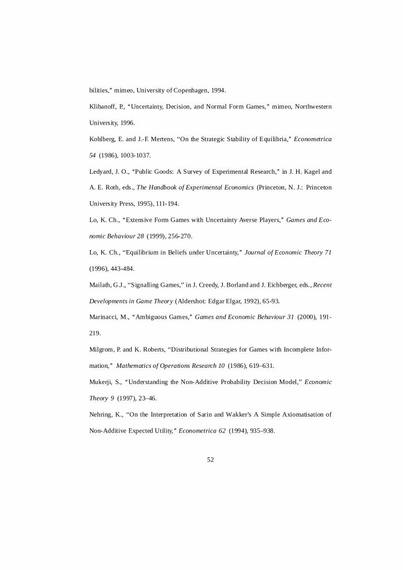
bilities,’’ mimeo, University of Copenhagen, 1994.

Klibanoff, P., ‘‘Uncertainty, Decision, and Normal Form Games,’’ mimeo, Northwestern

University, 1996.

Kohlberg, E. and J.-F. Mertens, ‘‘On the Strategic Stability of Equilibria,’’ Econometrica

54 (1986), 1003-1037.

Ledyard, J. O., ‘‘Public Goods: A Survey of Experimental Research,’’ in J. H. Kagel and

A. E. Roth, eds., The Handbook of Experimental Economics (Princeton, N. J.: Princeton

University Press, 1995), 111-194.

Lo, K. Ch., ‘‘Extensive Form Games with Uncertainty Averse Players,’’ Games and Eco-

nomic Behaviour 28 (1999), 256-270.

Lo, K. Ch., ‘‘Equilibrium in Beliefs under Uncertainty,’’ Journal of Economic Theory 71

(1996), 443-484.

Mailath, G.J., ‘‘Signalling Games,’’ in J. Creedy, J. Borland and J. Eichberger, eds., Recent

Developments in Game Theory (Aldershot: Edgar Elgar, 1992), 65-93.

Marinacci, M., ‘‘Ambiguous Games,’’ Games and Economic Behaviour 31 (2000), 191-

219.

Milgrom, P. and K. Roberts, ‘‘Distributional Strategies for Games with Incomplete Infor-

mation,’’ Mathematics of Operations Research 10 (1986), 619–631.

Mukerji, S., ‘‘Understanding the Non-Additive Probability Decision Model,’’ Economic

Theory 9 (1997), 23–46.

Nehring, K., ‘‘On the Interpretation of Sarin and Wakker’s A Simple Axiomatisation of

Non-Additive Expected Utility,’’ Econometrica 62 (1994), 935–938.

52

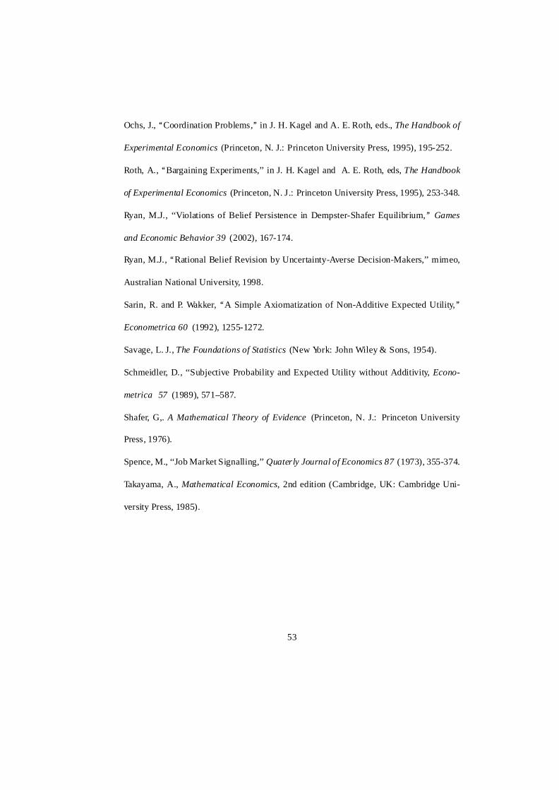
Ochs, J., ‘‘Coordination Problems,’’ in J. H. Kagel and A. E. Roth, eds., The Handbook of

Experimental Economics (Princeton, N. J.: Princeton University Press, 1995), 195-252.

Roth, A., ‘‘Bargaining Experiments,’’ in J. H. Kagel and A. E. Roth, eds, The Handbook

of Experimental Economics (Princeton, N. J.: Princeton University Press, 1995), 253-348.

Ryan, M.J., ‘‘Violations of Belief Persistence in Dempster-Shafer Equilibrium,’’ Games

and Economic Behavior 39 (2002), 167-174.

Ryan, M.J., ‘‘Rational Belief Revision by Uncertainty-Averse Decision-Makers,’’ mimeo,

Australian National University, 1998.

Sarin, R. and P. Wakker, ‘‘A Simple Axiomatization of Non-Additive Expected Utility,’’

Econometrica 60 (1992), 1255-1272.

Savage, L. J., The Foundations of Statistics (New York: John Wiley & Sons, 1954).

Schmeidler, D., ‘‘Subjective Probability and Expected Utility without Additivity, Econo-

metrica 57 (1989), 571–587.

Shafer, G,. A Mathematical Theory of Evidence (Princeton, N. J.: Princeton University

Press, 1976).

Spence, M., ‘‘Job Market Signalling,’’ Quaterly Journal of Economics 87 (1973), 355-374.

Takayama, A., Mathematical Economics, 2nd edition (Cambridge, UK: Cambridge Uni-

versity Press, 1985).

53

r

rr

rr

r

D

P

no

o

d

c¡1;¡1

1; 1

0; 3

Figure 1: Frivolous suit

54

r

r

r

r

r

r r

r

r

rr

r

2

2

r

r

r

r

r

r

2

2

0

12

12

t1

t2

L

L R

R

U

D

U

D

U

D

U

D

1; 1

1; 0

0; 1

0; 4

0; 1

0; 4

1; 1

1; 0

Figure 2: Ryan (2002)

55

q

q

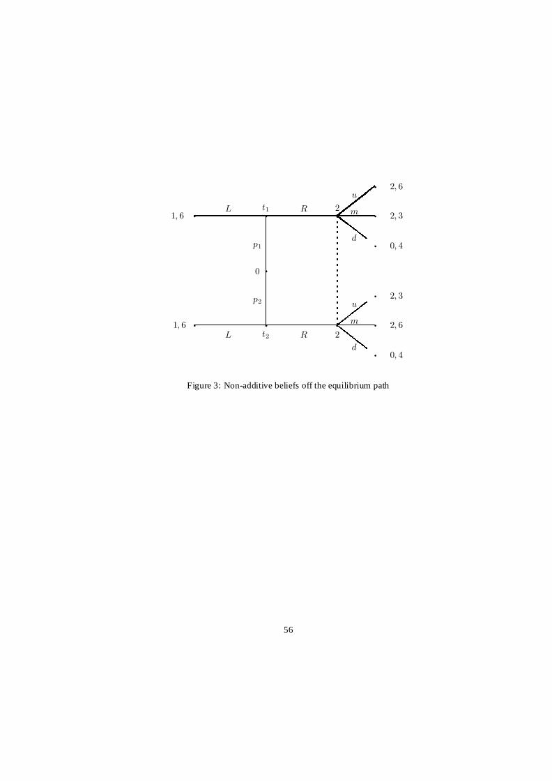
q

q

q

q q

q

q

qq

q

2

2

1; 6

1; 6

q

q

0

p2

t1

t2

L

L R

R

u

d

u

d

2; 6

0; 4

2; 3

0; 4

q

q

m

m 2; 6

2; 3

p1

Figure 3: Non-additive beliefs off the equilibrium path

56

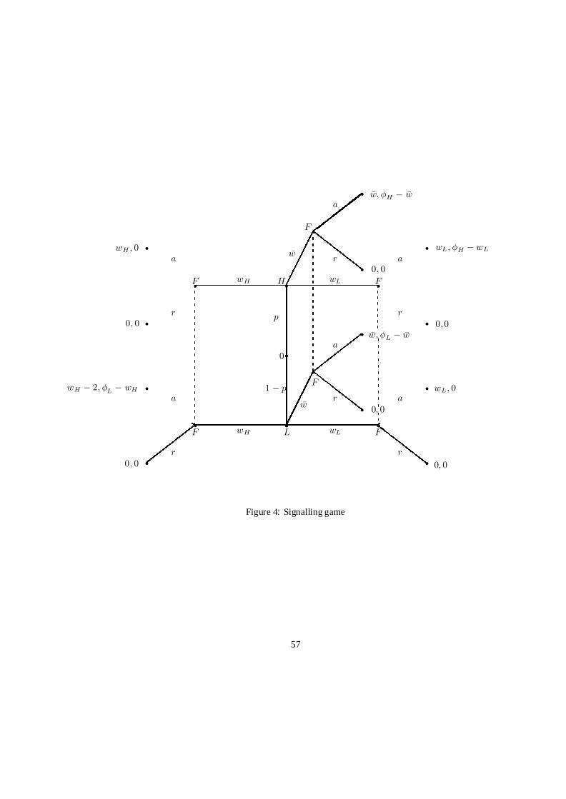
r

r

r

r

r

r r

r

r

rr

r

F

F

r

r

r

r

r

r

F

F

0

p

1 ¡ p

H

L

wH

wH wL

wL

a

r

a

r

a

r

a

r0; 0

r

rr

r

a

r

r

r

a

r

F

F

¹w

0; 0

¹w

0;0

wL; ÁH ¡ wL

wL; 0

0; 0

¹w; ÁL ¡ ¹w

0; 0

¹w; ÁH ¡ ¹w

wH ; 0

0; 0

wH ¡ 2; ÁL ¡ wH

Figure 4: Signalling game

57