U n i v e r s i t ä t A u g s b u r g

Institut fürMathematik

Dirk Blomker, Wael Wagih Mohammed

Amplitude Equations for SPDEs with Cubic Nonlinearities

Preprint Nr. 18/2010 — 07. Dezember 2010Institut fur Mathematik, Universitatsstraße, D-86135 Augsburg http://www.math.uni-augsburg.de/

Impressum:

Herausgeber:

Institut fur MathematikUniversitat Augsburg86135 Augsburghttp://www.math.uni-augsburg.de/pages/de/forschung/preprints.shtml

ViSdP:

Dirk BlomkerInstitut fur MathematikUniversitat Augsburg86135 Augsburg

Preprint: Samtliche Rechte verbleiben den Autoren c© 2010

Amplitude Equations for SPDEs

with Cubic Nonlinearities

Dirk Blomker∗ and Wael W. Mohammed†

Institut fur MathematikUniversitat Augsburg, Germany

November 29, 2010

Abstract

For a quite general class of SPDEs with cubic nonlinearities we deriverigorously amplitude equations describing the essential dynamics usingthe natural separation of time-scales near a change of stability. Typicalexamples are the Swift-Hohenberg equation, the Ginzburg-Landau (orAllen-Cahn) equation and some model from surface growth.

We discuss the impact of degenerate noise on the dominant behavior,and see that additive noise has the potential to stabilize the dynamics ofthe dominant modes. Furthermore, we discuss higher order corrections tothe amplitude equation.

1 Introduction

Stochastic partial differential equations (SPDEs) with cubic nonlinearity appearin several applications, for instance the Swift-Hohenberg equation, which wasfirst used as a toy model for the convective instability of fluids in the Rayleigh-Benard problem (see [3] or [7]). The simplest example is the well know realvalued Ginzburg-Landau equation, which depending on the underlying appli-cation is also called Allen-Cahn, Chaffee-Infante or nonlinear Heat equation.Moreover, we briefly discuss a model from surface growth proposed by Lai &Das Sarma (cf. [8] and see also [9]).

All equations considered in this article are parabolic nonlinear SPDEs per-turbed by additive forcing. Near a change of stability, we can use the naturalseparation of time-scales, in order to derive simpler equations for the evolutionof the dominant pattern. As these equations describe the amplitudes of domi-nant pattern, they are referred to as amplitude equations. When the order ofthe noise strength is comparable to the order of the distance from the change ofstability, the impact of noise can be seen. See for example [1] and the referencestherein.

∗e-mail: dirk.bloemker@math.uni-augsburg.de†e-mail: wael.mohammed@math.uni-augsburg.de

1

Recently the impact of degenerate noise not acting directly on the dominantpattern was studies for equations of Burgers type formally [10] and later rigor-ously [2]. Here noise is transported via nonlinear interaction to the dominantmodes.

Our current research was initiated by an observation of Axel Hutt and col-laborators [4, 5, 6]. Using numerical simulations and a formal argument basedon center manifold theory, they showed that noise constant in space leads to adeterministic amplitude equation, which is stabilized by the impact of additivenoise. This leads to a significant shift of the first pattern forming instability.The aim of this paper is to make these results rigorous.

Moreover, we want to study higher order corrections to the amplitude equa-tion, in order to see the fluctuations induced by the impact of the noise on thedominant pattern. Related results in this direction are discussed by Roberts &Wei [11], nevertheless their setting is slightly different, and they use averagingtechniques that do not lead to explicit error estimates.

The general prototype of equations under consideration is of the type

du(t) =[Au(t) + ε2Lu(t) + F(u(t))

]dt+ εdW (t), (1)

where A is non-positive self-adjoint operator with finite dimensional kernel,ε2Lu is a small deterministic perturbation, F is a cubic nonlinearity, and W issome finite dimensional Gaussian noise with small noise strength ε > 0. Notethat the small deterministic part, that reflects the distance from bifurcation,scales with ε. Different scalings are possible, but the one chosen here, is exactlythe one where noise and linear instability will interact in an interesting way.For simplicity of presentation, we will work in some Hilbert space H equippedwith scalar product 〈·, ·〉 and corresponding norm ‖ · ‖. Other norms like thesupremum-norm or the Lp-norm would lead to similar results.

Our aim of this paper is to establish rigorously an amplitude equation andtheir higher order corrections for this quite general class of SPDEs with cubicnonlinearities given by (1). In the examples we will show that additive degen-erate noise leads to stabilization of the solutions.

The paper is organized as follows. In the next section, we discuss the formalderivation of our results, while giving the precise assumptions and statementsof the main results in Section 3. Section 4 gives bounds on the non-dominantmodes, while Section 5 provides averaging results, in order to remove the im-pact of the higher modes on the dominant ones. In Section 6, we study theapproximation via amplitude equations, which is in the final Section 7 extendedto higher order corrections.

2 Formal Derivation

Before we proceed to give detailed assumptions, we present a short formalderivation and motivation of the main results. We will denote the kernel ofA by N := kerA. These are the dominant modes or the pattern that changestability. By S = N⊥ we denote the orthogonal complement in H. Further-more, denote by Pc the orthogonal projection Pc : H → N onto N and definePs := I − Pc, where I is the identity operator on H.

Here we study the behavior of solutions u of (1) on the natural slow time-scale of order ε−2, given by the distance from bifurcation.

2

So, we consider u on the slow time and split it into the dominant part a ∈ Nand the orthogonal part ψ ∈ S.

u(t) = εa(ε2t) + εψ(ε2t) (2)

Rescaling a and ψ to the slow time-scale T = ε2t, leads to the following systemof equations:

da =[ε−2Aca+ Lca+ Lcψ + Fc(a+ ψ)

]dT + ε−1dWc , (3)

anddψ =

[ε−2Asψ + Lsa+ Lsψ + Fs(a+ ψ)

]dT + ε−1dWs , (4)

where W (T ) := εW (ε−2T ) is a rescaled version of the driving Wiener processW . For short-hand notation, we use the subscripts c and s for projection ontoN and S, i.e., Ac = PcA and As = PsA, for short.

Let us suppose that the projections Pc and Ps commute not only with A,but also with L. Moreover suppose that the noise is degenerate and acts onlyon S. Then the system (3)-(4) takes the form

da = [Lca+ Fc(a+ ψ)] dT, (5)

anddψ =

[ε−2Asψ + Lsψ + Fs(a+ ψ)

]dT + ε−1dWs . (6)

Formally, in first approximation we immediately see that ψ is a fast Ornstein-Uhlenbeck process (OU, for short) given by the linear equation

dψ = ε−2AsψdT + ε−1dWs .

The rigorous statement can be found in Lemma 13.Thus we can eliminate ψ in Equation (5) by explicitly averaging over the

fast modes. In order to derive error estimates this procedure will be based onthe Ito-Formula (see Lemma 17). Usually, in most applications of averaging, wecan only hope for weak convergence in law without any error bound.

2.1 The Impact of Noise

Let us discuss the averaging and the impact of the noise in some more detailhere. Consider for simplicity of the argument here instead of ψ some real valuedfast OU-process Z given by

Z(T ) := αε−1∫ T

0

e−ε−2λ(T−τ)dβ(τ), (7)

where β(T ) := εβ(ε−2T ) denotes a rescaled version of a Brownian motion β onthe fast time-scale.

We apply Ito formula to Z and Z2, in order to obtain

ZdT =αε

λdβ − ε2

λdZ.

and

Z2dT =α2

2λdT +

εα

λZdβ − ε2

2λdZ2

3

Thus, on the slow time-scale T we can suppose that in integrals the process Zis small due to averaging, and a square of Z can be replaced by a constant. SeeLemma 17 for a rigorous statement. Note that the next order corrections (orderε) are always stochastic integrals and thus martingales.

We see later in Lemma 14 that for the fast OU-processes Z = O(ε−κ0) forarbitrarily small κ0 > 0. Thus we obtain formally that Z is a white noise onthe slow time scale:

Z(T ) = εα

λ∂T β + error,

where this error is small only in the sense of distributions, for example in H−1.

2.2 Amplitude Equation

One main result of the paper is the following approximation by amplitude equa-tions. Suppose for simplicity that the initial condition is sufficiently small, thenwe obtain for u

u(t) ' εb(ε2t) + εZ(ε2t) +O(ε2−), (8)

where Z is a fast OU-process and b is the solution of the amplitude equation onthe slow time-scale

∂T b = Lcb+ Fc(b) +

N∑k=n+1

3α2k

2λkFc(b, ek, ek) . (9)

The exact form of the additional linear terms is discussed later. The OU processZ is noise of order ε, as discussed in Section 2.1 before.

To illustrate this approximation result stated later in Theorem 9, we discusshere (similar to [6] the Swift-Hohenberg equation subject to periodic boundaryconditions on [0, 2π] forced by spatially constant noise:

∂tu = −(1 + ∂2x)2u+ νε2u− u3 + εα∂tβ. (10)

Rescaling the solution u of (10) to the slow time-scale by u(t) = εv(ε2t), ourmain theorem in this case (cf. Theorem 9) states that v is of the type

v ' γ1 sin +γ−1 cos +εα√2π∂T β +O(ε1−),

where γ1 and γ−1 are the solutions of the amplitude equations

∂T γi = (ν − 3α2

4π )γi − 34γi(γ

21 + γ2−1) for i = ±1.

We note that if α is large compared to ν, then (ν− 3α2

4π ) is negative. In this casethe degenerate additive noise stabilizes the dynamics of the dominant modes.

2.3 Higher order Corrections

The second main results studies the higher order correction for the solution ofequation (1). As indicated for the fast OU-process in Section 2.1, we obtainadditional Martingale terms that lead to additive noise in an equation for thehigher order correction of the amplitude, but the strength of the noise dependson the first order approximation. Unfortunately, as we rely on a Martingale

4

representation argument of [2], we are limited in the final argument to one-dimensional dominant spaces, i.e. dimN = 1. Nevertheless, it is possible tocarry over the results to higher dimensional N , if we only ask for weak conver-gence of the approximation.

If we consider higher order corrections to (8), we obtain additional martingaleterms of order ε in (9) from the Ito-formula argument. These terms depend onb and the fast OU-process. Further averaging arguments are necessary.

We now improve the approximation of (1) from (8) by including a higherorder term:

u(t) ' εb1(ε2t) + ε2b2(ε2t) + εZ(ε2t) +O(ε3−), (11)

where b1 is again the solution of the amplitude equation (9). Later we will seethat b2 is the solution of

db2 = [Lcb2 + 3Fc(b2, b1, b1) +

N∑k=2

3σ2

2λkFc(b2, ek, ek)]dT + dMb1 , (12)

where Mb1(T ) is a martingale defined by

Mb1(T ) =

∫ T

0

( N∑k=2

gk(b1)) 1

2

dB(s) , (13)

where the integration is against a one-dimensional Brownian motion B aris-ing from a martingale representation argument (cf. Lemma 34). The gk’s arepolynomials of degree 4 in b1 given later in (74).

3 Assumptions and main results

This section summarizes all assumptions necessary for our results. For the linearoperator A in (1) on the Hilbert-space H we assume the following:

Assumption 1 (Linear operator A) Suppose A is a non-positive operator onH with eigenvalues 0≤λ1≤ . . .≤λk≤ . . . and λk ≥ Ckm for all sufficiently largek, and a complete orthonormal system of eigenvectors ek∞k=1 such that Aek =−λkek. Suppose that N := kerA has finite dimension n with basis (e1, . . . , en) .

As before, we denote by Pc the orthogonal projection onto N and by Ps theorthogonal projection onto the orthogonal complement S = N⊥.

Definition 2 (spaces Hα) For α ∈ R, we define the space Hα as

Hα = ∞∑k=1

γkek :

∞∑k=1

γ2kk2α <∞

with norm

∥∥∥ ∞∑k=1

γkek

∥∥∥2α

=( ∞∑k=1

γ2kk2α)1/2

.

The operator A given by Assumption 1 generates an analytic semigroupetAt≥0 defined by

eAt( ∞∑k=1

γkek

)=

∞∑k=1

e−λktγkek ∀ t ≥ 0,

5

and has the following property for all t > 0, β ≥ α, λn < c ≤ λn+1 and allu ∈ Hβ ∥∥etAPsu∥∥α ≤Mt−

α−βm e−ct ‖Psu‖β , (14)

where M depends only on α, β and c.

Assumption 3 (Operator L) Let L : Hα → Hα−β for some β ∈ [0,m) be alinear continuous mapping that commutes with Pc and Ps.

For the nonlinearity F we assume that:

Assumption 4 (nonlinearity F) Assume that F : (Hα)3 → Hα−β with β as

in Assumption 3 is trilinear, symmetric and satisfies the following conditions,for some C > 0,

‖F(u, v, w)‖α−β ≤ C‖u‖α‖v‖α‖w‖α ∀ u, v, w ∈ Hα, (15)

〈Fc(u), u〉 ≤ 0 ∀ u ∈ N , (16)

and〈Fc(u, u, w), w〉 ≤ 0 ∀ u, w ∈ N . (17)

We use F(u) = F(u, u, u) and Fc = PcF for shorthand notation.For the noise we suppose:

Assumption 5 (Wiener process W ) Let W be a Wiener process in H oversome probability space (Ω,z,P). Suppose for t ≥ 0,

W (t) =

N∑k=n+1

αkβk(t)ek for some N ≥ n+ 1,

where (βk)k are independent, standard Brownian motions in R and (αk)k arereal numbers.

Remark 6 We take N < ∞ in the above assumption for simplicity of presen-tation. Nevertheless most results are still true for N = ∞, if we control theconvergence of various infinite series, i.e. for αk decaying sufficiently fast fork →∞.

We define the fast OU processes Z and Zk(T ) by

Zk(T ) := αkε−1∫ T

0

e−ε−2λk(T−τ)dβk(τ), (18)

for k ∈ n+ 1, . . . , N and

Z(T ) :=

N∑k=n+1

Zk(T )ek , (19)

where βk(T ) := εβk(ε−2T ) is a rescaled version of the Brownian motion.For our result we rely on a cut off argument. We consider only solutions

u = (a, ψ) that are not too large, as given by the next definition.

6

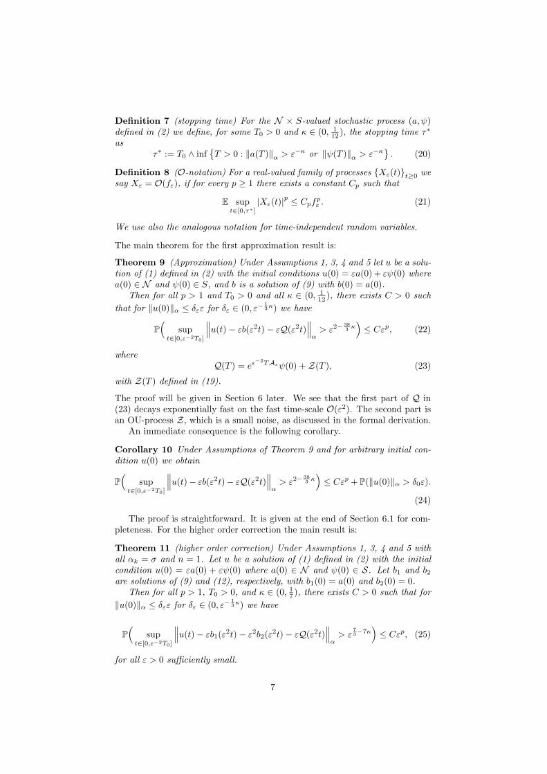
Definition 7 (stopping time) For the N × S-valued stochastic process (a, ψ)defined in (2) we define, for some T0 > 0 and κ ∈ (0, 1

12 ), the stopping time τ∗

asτ∗ := T0 ∧ inf

T > 0 : ‖a(T )‖α > ε−κ or ‖ψ(T )‖α > ε−κ

. (20)

Definition 8 (O-notation) For a real-valued family of processes Xε(t)t≥0 wesay Xε = O(fε), if for every p ≥ 1 there exists a constant Cp such that

E supt∈[0,τ∗]

|Xε(t)|p ≤ Cpfpε . (21)

We use also the analogous notation for time-independent random variables.

The main theorem for the first approximation result is:

Theorem 9 (Approximation) Under Assumptions 1, 3, 4 and 5 let u be a solu-tion of (1) defined in (2) with the initial conditions u(0) = εa(0) + εψ(0) wherea(0) ∈ N and ψ(0) ∈ S, and b is a solution of (9) with b(0) = a(0).

Then for all p > 1 and T0 > 0 and all κ ∈ (0, 112 ), there exists C > 0 such

that for ‖u(0)‖α ≤ δεε for δε ∈ (0, ε−13κ) we have

P(

supt∈[0,ε−2T0]

∥∥∥u(t)− εb(ε2t)− εQ(ε2t)∥∥∥α> ε2−

383 κ)≤ Cεp, (22)

whereQ(T ) = eε

−2TAsψ(0) + Z(T ), (23)

with Z(T ) defined in (19).

The proof will be given in Section 6 later. We see that the first part of Q in(23) decays exponentially fast on the fast time-scale O(ε2). The second part isan OU-process Z, which is a small noise, as discussed in the formal derivation.

An immediate consequence is the following corollary.

Corollary 10 Under Assumptions of Theorem 9 and for arbitrary initial con-dition u(0) we obtain

P(

supt∈[0,ε−2T0]

∥∥∥u(t)− εb(ε2t)− εQ(ε2t)∥∥∥α> ε2−

383 κ)≤ Cεp + P(‖u(0)‖α > δ0ε).

(24)

The proof is straightforward. It is given at the end of Section 6.1 for com-pleteness. For the higher order correction the main result is:

Theorem 11 (higher order correction) Under Assumptions 1, 3, 4 and 5 withall αk = σ and n = 1. Let u be a solution of (1) defined in (2) with the initialcondition u(0) = εa(0) + εψ(0) where a(0) ∈ N and ψ(0) ∈ S. Let b1 and b2are solutions of (9) and (12), respectively, with b1(0) = a(0) and b2(0) = 0.

Then for all p > 1, T0 > 0, and κ ∈ (0, 17 ), there exists C > 0 such that for

‖u(0)‖α ≤ δεε for δε ∈ (0, ε−13κ) we have

P(

supt∈[0,ε−2T0]

∥∥∥u(t)− εb1(ε2t)− ε2b2(ε2t)− εQ(ε2t)∥∥∥α> ε

73−7κ

)≤ Cεp, (25)

for all ε > 0 sufficiently small.

7

The proof of this theorem will be given in Section 7 later. Again, with the sameproof as the previous corollary, we obtain:

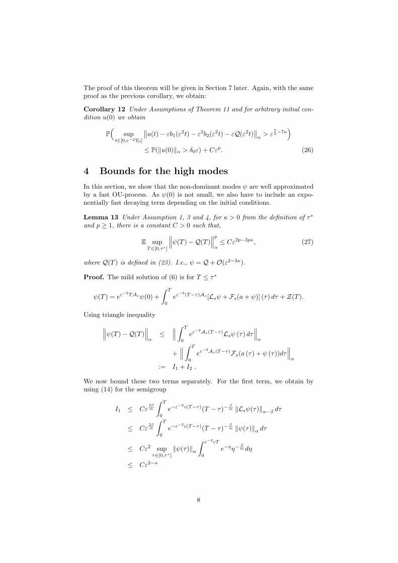
Corollary 12 Under Assumptions of Theorem 11 and for arbitrary initial con-dition u(0) we obtain

P(

supt∈[0,ε−2T0]

∥∥u(t)− εb1(ε2t)− ε2b2(ε2t)− εQ(ε2t)∥∥α> ε

73−7κ

)≤ P(‖u(0)‖α > δ0ε) + Cεp. (26)

4 Bounds for the high modes

In this section, we show that the non-dominant modes ψ are well approximatedby a fast OU-process. As ψ(0) is not small, we also have to include an expo-nentially fast decaying term depending on the initial conditions.

Lemma 13 Under Assumption 1, 3 and 4, for κ > 0 from the definition of τ∗

and p ≥ 1, there is a constant C > 0 such that,

E supT∈[0,τ∗]

∥∥∥ψ(T )−Q(T )∥∥∥pα≤ Cε2p−3pκ, (27)

where Q(T ) is defined in (23). I.e., ψ = Q+O(ε2−3κ).

Proof. The mild solution of (6) is for T ≤ τ∗

ψ(T ) = eε−2TAsψ(0) +

∫ T

0

eε−2(T−τ)As [Lsψ + Fs(a+ ψ)] (τ) dτ + Z(T ).

Using triangle inequality∥∥∥ψ(T )−Q(T )∥∥∥α≤

∥∥∥ ∫ T

0

eε−2As(T−τ)Lsψ (τ) dτ

∥∥∥α

+∥∥∥∫ T

0

eε−2As(T−τ)Fs(a (τ) + ψ (τ))dτ

∥∥∥α

:= I1 + I2 .

We now bound these two terms separately. For the first term, we obtain byusing (14) for the semigroup

I1 ≤ Cε2βm

∫ T

0

e−ε−2c(T−τ)(T − τ)−

βm ‖Lsψ(τ)‖α−β dτ

≤ Cε2βm

∫ T

0

e−ε−2c(T−τ)(T − τ)−

βm ‖ψ(τ)‖α dτ

≤ Cε2 supτ∈[0,τ∗]

‖ψ(τ)‖α∫ ε−2cT

0

e−ηη−βm dη

≤ Cε2−κ

8

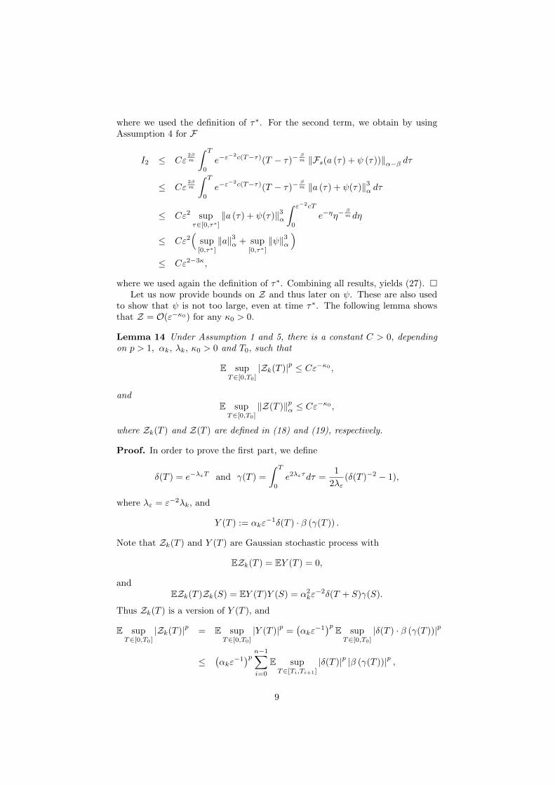
where we used the definition of τ∗. For the second term, we obtain by usingAssumption 4 for F

I2 ≤ Cε2βm

∫ T

0

e−ε−2c(T−τ)(T − τ)−

βm ‖Fs(a (τ) + ψ (τ))‖α−β dτ

≤ Cε2βm

∫ T

0

e−ε−2c(T−τ)(T − τ)−

βm ‖a (τ) + ψ(τ)‖3α dτ

≤ Cε2 supτ∈[0,τ∗]

‖a (τ) + ψ(τ)‖3α∫ ε−2cT

0

e−ηη−βm dη

≤ Cε2(

sup[0,τ∗]

‖a‖3α + sup[0,τ∗]

‖ψ‖3α)

≤ Cε2−3κ,

where we used again the definition of τ∗. Combining all results, yields (27). Let us now provide bounds on Z and thus later on ψ. These are also used

to show that ψ is not too large, even at time τ∗. The following lemma showsthat Z = O(ε−κ0) for any κ0 > 0.

Lemma 14 Under Assumption 1 and 5, there is a constant C > 0, dependingon p > 1, αk, λk, κ0 > 0 and T0, such that

E supT∈[0,T0]

|Zk(T )|p ≤ Cε−κ0 ,

andE supT∈[0,T0]

‖Z(T )‖pα ≤ Cε−κ0 ,

where Zk(T ) and Z(T ) are defined in (18) and (19), respectively.

Proof. In order to prove the first part, we define

δ(T ) = e−λεT and γ(T ) =

∫ T

0

e2λετdτ =1

2λε(δ(T )−2 − 1),

where λε = ε−2λk, and

Y (T ) := αkε−1δ(T ) · β (γ(T )) .

Note that Zk(T ) and Y (T ) are Gaussian stochastic process with

EZk(T ) = EY (T ) = 0,

andEZk(T )Zk(S) = EY (T )Y (S) = α2

kε−2δ(T + S)γ(S).

Thus Zk(T ) is a version of Y (T ), and

E supT∈[0,T0]

|Zk(T )|p = E supT∈[0,T0]

|Y (T )|p =(αkε

−1)p E supT∈[0,T0]

|δ(T ) · β (γ(T ))|p

≤(αkε

−1)p n−1∑i=0

E supT∈[Ti,Ti+1]

|δ(T )|p |β (γ(T ))|p ,

9

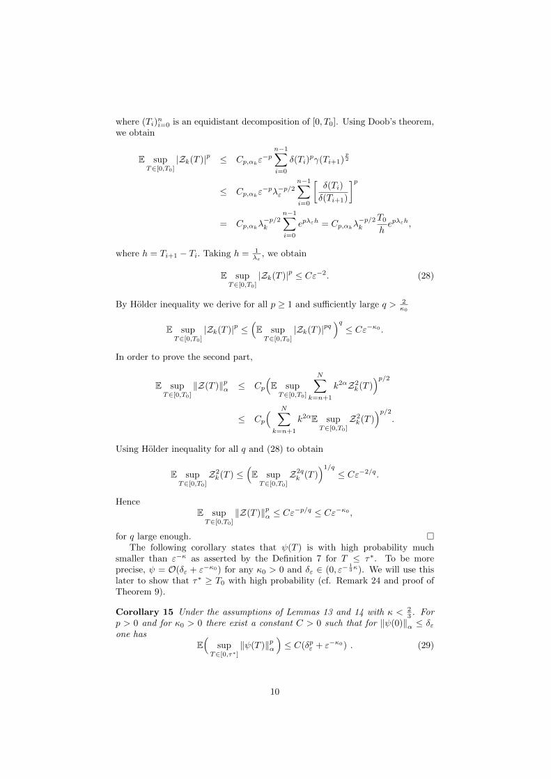
where (Ti)ni=0 is an equidistant decomposition of [0, T0]. Using Doob’s theorem,

we obtain

E supT∈[0,T0]

|Zk(T )|p ≤ Cp,αkε−p

n−1∑i=0

δ(Ti)pγ(Ti+1)

p2

≤ Cp,αkε−pλ−p/2ε

n−1∑i=0

[δ(Ti)

δ(Ti+1)

]p

= Cp,αkλ−p/2k

n−1∑i=0

epλεh = Cp,αkλ−p/2k

T0hepλεh,

where h = Ti+1 − Ti. Taking h = 1λε, we obtain

E supT∈[0,T0]

|Zk(T )|p ≤ Cε−2. (28)

By Holder inequality we derive for all p ≥ 1 and sufficiently large q > 2κ0

E supT∈[0,T0]

|Zk(T )|p ≤(E supT∈[0,T0]

|Zk(T )|pq)q≤ Cε−κ0 .

In order to prove the second part,

E supT∈[0,T0]

‖Z(T )‖pα ≤ Cp

(E supT∈[0,T0]

N∑k=n+1

k2αZ2k(T )

)p/2≤ Cp

( N∑k=n+1

k2αE supT∈[0,T0]

Z2k(T )

)p/2.

Using Holder inequality for all q and (28) to obtain

E supT∈[0,T0]

Z2k(T ) ≤

(E supT∈[0,T0]

Z2qk (T )

)1/q≤ Cε−2/q.

HenceE supT∈[0,T0]

‖Z(T )‖pα ≤ Cε−p/q ≤ Cε−κ0 ,

for q large enough. The following corollary states that ψ(T ) is with high probability much

smaller than ε−κ as asserted by the Definition 7 for T ≤ τ∗. To be moreprecise, ψ = O(δε + ε−κ0) for any κ0 > 0 and δε ∈ (0, ε−

13κ). We will use this

later to show that τ∗ ≥ T0 with high probability (cf. Remark 24 and proof ofTheorem 9).

Corollary 15 Under the assumptions of Lemmas 13 and 14 with κ < 23 . For

p > 0 and for κ0 > 0 there exist a constant C > 0 such that for ‖ψ(0)‖α ≤ δεone has

E(

supT∈[0,τ∗]

‖ψ(T )‖pα)≤ C(δpε + ε−κ0) . (29)

10

Proof. From (27), by triangle inequality and Lemma 14, we obtain

E(

supT∈[0,τ∗]

‖ψ(T )‖pα)≤ Cδpε + Cε−κ0 + Cε2p−3pκ,

for κ < 23 we obtain (29).

Lemma 16 If Assumption 1 holds, then for q ≥ 1 there exists a constant C > 0such that for ‖ψ(0)‖α ≤ δε one has∫ T

0

∥∥∥eτε−2Asψ(0)∥∥∥qαdτ ≤ Cδqεε2.

Proof. Using (14) we obtain∫ T

0

∥∥∥eε−2Asτψ(0)∥∥∥qαdτ ≤ c

∫ T

0

e−qε−2cτ ‖ψ(0)‖qα dτ ≤

ε2

qc‖ψ(0)‖qα .

5 Averaging over the fast OU-process

Let us not turn to the averaging result. First in 17, we provide the first orderapproximation, while in Lemma 18 we state all corrections of order ε.

Lemma 17 Let X be a real valued stochastic process such that for some r ≥ 0we have X(0) = O(ε−r). Fix any κ0 > 0. If dX = GdT with G = O(ε−r),then, for any non-negative integers n1 , n2 , n3 not all zero and for all triples ofdifferent indices k1, k2, k3 ∈ n+ 1, . . . , N, we obtain

T∫0

XZn1

k1Zn2

k2Zn3

k3dτ =

3∑i=1

ni(ni − 1)α2ki

2(n1λk1 + n2λk2 + n3λk3)

T∫0

XZn1

k1Zn2

k2Zn3

k3Z−2ki dτ

+O(ε1−r−(n1+n2+n3)κ0), (30)

where the fast OU-process Zk is defined in (18).

Proof. We note first that

E sup[0,T0]

|X|p ≤ CE sup[0,T0]

|G|p ≤ Cε−pr.

11

Applying Ito formula to XZn1

k Zn2

l Zn3j and integrating from 0 to T in order to

obtain (note that the β’s are independent, thus dβkdβl = 0 if k 6= l)

(n1λk + n2λl + n3λj)

T∫0

XZn1

k Zn2

l Zn3j dτ

= −ε2X(T )Zn1

k (T )Zn2

l (T )Zn3j (T ) + ε2

T∫0

Zn1

k Zn2

l Zn3j Gdτ

+n1αkε

T∫0

XZn1−1k Zn2

l Zn3j dβk + n2αlε

T∫0

XZn1

k Zn2−1l Zn3

j dβl

+n3αjε

T∫0

XZn1

k Zn2

l Zn3−1j dβj +

n1(n1 − 1)α2k

2

T∫0

XZn1−2k Zn2

l Zn3j dτ

+n2(n2 − 1)α2

l

2

T∫0

XZn1

k Zn2−2l Zn3

j dτ +n3(n3 − 1)α2

j

2

T∫0

XZn1

k Zn2

l Zn3−2j dτ.

Taking the absolute value and using Burkholder-Davis-Gundy theorem yields(30).

We can also give the higher order correction terms.

Lemma 18 Under assumption of Lemma 17, we have

T∫0

XZn1

k1Zn2

k2Zn3

k3dτ =

3∑i=1

ni(ni − 1)α2ki

2(n1λk1 + n2λk2 + n3λk3)

T∫0

XZn1

k1Zn2

k2Zn3

k3Z−2ki dτ

+ε

3∑i=1

niαkin1λk1 + n2λk2 + n3λk3

T∫0

XZn1

k1Zn2

k2Zn3

k3Z−1ki dβki

+O(ε2−r−(n1+n2+n3)κ0).

Proof. We follow the same proof, as in the previous Lemma.

Remark 19 Both Lemmas above are still true, in case X is a stochastic processin N or C.

6 First order estimates

This section is devoted to the proof of the first main result of Theorem 9. Inthe second part of this section we give some applications for this approximationresult.

6.1 Proof of the main result

Let us first check, that we can apply the averaging lemma to (5).

12

Lemma 20 Assume that Assumption 3 and 4 hold. Let X be a stochasticprocess in N and dX = GdT . If X = Fc(a, ek, el) or X = Fc(a, a, ek), thenG = O(ε−3κ) or G = O(ε−4κ), respectively.

Proof. If X = Fc(a, ek, ek), then

dX = Fc(da, ek, el) = Fc(Lca+ Fc(a+ ψ), ek, el)dT.

LetG = Fc(Lca+ Fc(a+ ψ), ek, el).

Taking the Hα norm, using Assumption 4 and the fact all Hα-norms are equiv-alent on N , to obtain

‖G‖α ≤ C ‖Lca+ Fc(a+ ψ)‖α ≤ C ‖a‖α + C ‖Fc(a+ ψ)‖α−β≤ C ‖a‖α + C ‖a+ ψ‖3α ≤ C ‖a‖α + C ‖a‖3α + C ‖ψ‖3α .

Using the definition of τ∗, we obtain for p > 0

E sup[0,τ∗]

‖G‖pα ≤ Cε−3pκ.

Analogously, if X = Fc(a, a, ek), then

dX = 2Fc(da, a, ek) = 2Fc(Lca+ Fc(a+ ψ), a, ek)dT.

DefineG := 2Fc(Lca+ Fc(a+ ψ), a, ek),

in order to obtainE sup

[0,τ∗]

‖G‖pα ≤ Cε−4pκ.

Lemma 21 If Assumptions 1, 3, 4 and 5 hold and ‖ψ(0)‖α ≤ δε for δε ∈(0, ε−

13κ), for κ ∈ (0, 12 ) from the definition of τ∗, then

a(T ) = a(0) +

T∫0

Lca(τ)dτ +

T∫0

Fc(a)dτ +

N∑k=n+1

3α2k

2λk

T∫0

Fc(a, ek, ek)dτ +R(T ),

(31)where

R = O(ε1−5κ). (32)

Proof. Recall Lemma 13, which states

ψ = yε + Z +O(ε2−3κ), (33)

whereyε(T ) = eε

−2TAsψ(0).

13

Substituting from (33) into (5) we obtain for κ < 2/3 using the bounds fora = O(ε−κ), Z = O(ε−κ0), and yε = O(δεε

2)

da = [Lca+ Fc(a+ yε + Z)] dT +O(ε2−5κ)dT

= [Lca+ Fc(a) + 3Fc(a, a,Z) + 3Fc(a,Z,Z) + Fc(Z)

+3Fc(a, a, yε) + 6Fc(a,Z, yε) + 3Fc(Z,Z, yε)+3Fc(a, yε, yε) + 3Fc(Z, yε, yε) + Fc(yε)]dT +O(ε2−5κ)dT.

Integrating from 0 to T yields for T ≤ τ∗

a(T ) = a(0) +

T∫0

Lca(τ)dτ +

T∫0

Fc(a)dτ + 3

N∑k=n+1

T∫0

ZkFc(a, a, ek)dτ

+3

N∑k=n+1

T∫0

Z2kFc(a, ek, ek)dτ + 3

N∑k=n+1

N∑l 6=k

T∫0

ZkZlFc(a, ek, el)dτ

+

N∑k,l,j=n+1

T∫0

Fc(Zkek,Zlel,Zjej)dτ +R1 +O(ε2−5κ), (34)

where

R1 = 3

T∫0

Fc(a, a, yε)dτ + 6

T∫0

Fc(a,Z, yε)dτ + 3

T∫0

Fc(a, yε, yε)dτ

+3

T∫0

Fc(Z, yε, yε)dτ + 3

T∫0

Fc(Z,Z, yε)dτ + 3

T∫0

Fc(yε)dτ

:= I1 + I2 + I3 + I4 + I5 + I6. (35)

Now we use Assumption 3, the definition of τ∗, and the equivalence ofHα-normson N to bound R1. We bound all terms in (35) separately. For the first term in(35)

‖I1‖α ≤ CT∫

0

‖a‖2α ‖yε‖α dτ ≤ C sup[0,T0]

‖a‖2α

T∫0

‖yε‖α dτ.

Using Lemma 16 for q = 1, we obtain

I1 = O(δεε2−2κ).

Analogous results hold for all other terms. To be more precise:

I2 = O(δεε2−κ−κ0), I3 = O(δ2εε

2−κ), I4 = O(δ2εε2−κ0),

I5 = O(δεε2−2κ0), I6 = O(δ3εε

2) .

Collecting all results we obtain for κ0 ≤ κ, where κ0 > 0 is arbitrary fromLemma 14,

R1 = O((1 + δ2ε)ε2−2κ). (36)

Finally, applying Lemmas 17 and 20 to (34), we obtain (31).

14

Lemma 22 Let Assumptions 1, 3 and 4 hold. Define b in N as the solution of(9). If the initial condition satisfies E |b(0)|p ≤ δpε for δε ∈ (0, ε−

13κ), then for

all T0 > 0 there exists a constant C > 0 such that

supT∈[0,T0]

‖b(T )‖ ≤ C|b(0)|

E supT∈[0,T0]

|b(T )|p ≤ Cpδpε . (37)

Proof. Taking the scalar product 〈·, b〉 on both sides of (9) yields

1

2∂T |b|2 = 〈Lcb, b〉+ 〈Fc(b), b〉+

N∑k=n+1

3α2k

2λk〈Fc(b, ek, ek), b〉 .

Using Cauchy-Schwarz inequality and Assumption 4, we obtain

1

2∂T |b|2 ≤ C |b|2 .

We apply now a comparison argument to deduce for all T ∈ [0, T0]

|b(T )| ≤ |b(0)| eCT0 . (38)

Taking expectation after supremum on both sides yields (37). In the following we are no longer able to calculate moments of error terms.

Thus we restrict ourselves to a sufficiently large subset of Ω, where our estimatesgo through.

Definition 23 Given δε ∈ (0, ε−13κ) with κ > 0 from the definition of τ∗.

Define the set Ω∗ ⊂ Ω of all ω ∈ Ω such that all these estimates

sup[0,τ∗]

‖ψ −Q‖α < Cε2−4κ , (39)

sup[0,τ∗]

‖ψ‖α < δ0 + ε−12κ , (40)

sup[0,τ∗]

|R| < ε1−6κ , (41)

andsup[0,τ∗]

|b| < δ0ε− 1

2κ , (42)

hold.

Remark 24 The set Ω∗ has approximately probability 1. For this consider

P(Ω∗) ≥ 1− P( sup[0,τ∗]

‖ψ −Q‖α ≥ ε2−4κ)− P( sup[0,τ∗]

‖ψ‖α ≥ δε + ε−12κ)

−P( sup[0,τ∗]

|b| ≥ δεε−12κ)− P( sup

[0,τ∗]

|R| ≥ ε1−6κ).

Using Chebychev inequality and Lemmas 13, 21, 22 and Corollary 15 with δε <ε−

13κ, and some κ0 ≤ 1

3κ, we obtain for sufficient large q

P(Ω∗) ≥ 1− C[εqκ + ε12 qκ−qκ0 + ε

12 qκ + εqκ] ≥ 1− Cε 1

6 qκ ≥ 1− Cεp. (43)

15

Theorem 25 Assume that Assumptions 1, 3, 4 and 5 hold and suppose |a(0)| ≤δε and ‖ψ(0)‖α ≤ δε. Let b be a solution of the amplitude equation (9) and a asdefined in (2). If the initial conditions satisfy a(0) = b(0), then

supT∈[0,τ∗]

|a(T )− b(T )| ≤ C(1 + δ2ε)ε1−12κ, (44)

and for κ < 112

supT∈[0,τ∗]

|a(T )| ≤ C(1 + δ2ε), (45)

on Ω∗.

Proof. Define ϕ := a−R, where R is defined in (32). From (31) we obtain

ϕ(T ) = a(0)+

T∫0

Lc[ϕ+R]dτ+

T∫0

Fc(ϕ+R)dτ+

N∑k=n+1

3α2k

2λk

T∫0

Fc(ϕ+R, ek, ek)dτ.

(46)Subtracting (46) from the amplitude equation (9) and defining h := b − ϕ, weobtain

h(T ) =

T∫0

Lchdτ −T∫

0

LcRdτ +

T∫0

[Fc(b)−Fc(b− h+R)] dτ

+

N∑k=n+1

3α2k

2λk

T∫0

Fc(h−R, ek, ek)dτ.

Thus

∂Th = Lch−LcR+Fc(b)−Fc(b− h+R) +

N∑k=n+1

3α2k

2λkFc(h−R, ek, ek). (47)

Taking the scalar product 〈·, h〉 on both sides of (47), we have

1

2∂T |h|2 = 〈∂Th, h〉 = 〈Lch, h〉 − 〈LcR, h〉+ 〈Fc(b)−Fc(b− h+R), h〉

+

N∑k=n+1

3α2k

2λk〈Fc(h, ek, ek), h〉 −

N∑k=n+1

3α2k

2λk〈Fc(R, ek, ek), h〉 .

Using Cauchy-Schwarz inequality and Assumption 4, we obtain the followingdifferential inequality

∂T |h|2 ≤ C[|h|2 + |h|4] + C[|R|4 + |b|2|R|2 + |b|4|R|2 + |b|2|R|4

].

Using (41) and (42) in the definition of Ω∗, we obtain for T ≤ τ∗

∂T |h|2 ≤ C[|h|2 + |h|4] + C(1 + δ4ε)ε2−24κ on Ω∗.

As long as |h| ≤ 1, we obtain

∂T |h|2 ≤ 2C[|h|2 + C(1 + δ4ε)ε2−24κ.

16

Using Gronwall’s Lemma, we obtain for T ≤ τ∗ ≤ T0

|h(T )|2 ≤ C(1 + δ4ε)ε2−24κ ≤ 1,

for δε < ε−13κ with κ < 1

12 and ε > 0 sufficiently small. Thus

sup[0,τ∗]

|h| ≤ C(1 + δ20)ε1−12κ on Ω∗. (48)

We finish the first part by using (41), (48) and

sup[0,τ∗]

|a− b| = sup[0,τ∗]

|h−R| ≤ sup[0,τ∗]

|h|+ sup[0,τ∗]

|R| .

For the second part of the theorem consider

sup[0,τ∗]

|a| ≤ sup[0,τ∗]

|a− b|+ sup[0,τ∗]

|b|.

Using the first part and (42), we obtain (45) as κ < 112 .

Now, we can use the results previously obtained to prove the main result ofTheorem 9 for the approximation of the solution (8) of the SPDE (1).

Proof of Theorem 9. For the stopping time, we note that provided δε < ε−13κ

Ω ⊃ τ∗ = T0 ⊇ supT∈[0,T0]

|a(T )| < ε−κ, supT∈[0,T0]

‖ψ(T )‖α < ε−κ ⊇ Ω∗,

where the last inclusion holds due to (40) and Theorem 25. Now let us turn tothe approximation result. Using (2) and the triangle inequality yields on Ω∗

supT∈[0,τ∗]

∥∥∥u(ε−2T )− εb(T )− εQ(T )∥∥∥α≤ ε sup

[0,τ∗]

‖a− b‖α + ε sup[0,τ∗]

∥∥∥ψ −Q∥∥∥α

≤ C(1 + δ2ε)ε2−12κ + Cε3−4κ .

From (39) and (44), we obtain

supt∈[0,ε−2T0]

∥∥∥u(t)− εb(ε2t)− εQ(ε2t)∥∥∥α

= supt∈[0,ε−2τ∗]

∥∥∥u(t)− εb(ε2t)− εQ(ε2t)∥∥∥α

≤ Cε2−383 κ on Ω∗.

Thus

P(

supt∈[0,ε−2T0]

∥∥∥u(t)− εb(ε2t)− εQ(ε2t)∥∥∥α> ε2−

383 κ)≤ 1− P(Ω∗).

Using (43), yields (22). Proof of Corollary 10. Define Ω0 ⊂ Ω as

Ω0 = ω ∈ Ω : ‖u(0)‖α ≤ δ0ε,

and define

u(0) =

0 on Ωc0

u(0) on Ω0.

17

Hence, the solutions u and u corresponding to the initial conditions u(0) andu(0) coincide on Ω0. Thus

P(

supt∈[0,ε−2T0]

‖u(t)− εb(ε2t)− εQ(ε2t)‖α > ε2−383 κ)

= P(

supt∈[0,ε−2T0]

‖u(t)− εb(ε2t)− εQ(ε2t)‖α > ε2−383 κ∩ Ω0

)+P(

supt∈[0,ε−2T0]

‖u(t)− εb(ε2t)− εQ(ε2t)‖α > ε2−383 κ∩ Ωc0

)≤ P

(sup

t∈[0,ε−2T0]

‖u(t)− εb(ε2t)− εQ(ε2t)‖α > ε2−383 κ)

+ P(

Ωc0

)≤ Cεp + P (‖u(0)‖α > δεε) ,

where we used (22) for the solution u.

6.2 Applications

In the literature there are numerous examples of equations with cubic nonlin-earities where our theory does apply. Examples are Swift-Hohenberg equation,Ginzburg-Landau / Allen-Cahn equation and some Surface growth model. Inall these examples we obtain that adding noise stabilizes the dynamics of thedominant modes and the amplitude equation is always the following type

∂TA = νA− CαA− CFA|A|2,

where A is the amplitude of the dominant modes inN . The constant Cα dependsexplicitly on the noise strength, while CF depends only on the nonlinearity andthe linear operators in the equation.

6.2.1 Swift-Hohenberg equation

The Swift-Hohenberg equation was already defined in the introduction (cf.(10)). It has been used as a toy model for the convective instability in Rayleigh-Benard problem (see [3] or [7]). Now it is one of the celebrated models in thetheory of pattern formation [3]. For this model note that

A = −(1 + ∂2x)2, L = νI, F(u) = −u3.

If we take the orthonormal basis

ek(x) =

1√π

sin(kx) if k > 0,1√2π

if k = 0,1√π

cos(kx) if k < 0,

and the spaces

H = L2([0, 2π]) and N = spansin, cos,

then the eigenvalues of −A = (1 + ∂2x)2 are λk = (1 − k2)2 for k ∈ Z. So, itis easy to check that, after rearranging the indices, Assumption 1 is true withm = 4.

18

If we consider u = u1 sin +u−1 cos and w = w1 sin +w−1 cos ∈ N , then wecan easily verify Assumption 4 as follows:

〈Fc(u), u〉 = −3π

4(u21 + u2−1)2 ≤ 0,

where we used

Fc(u) = − 34 (u31 + u1u

2−1) sin− 3

4 (u3−1 + u21u−1) cos,

Moreover,

〈Fc(u, u, w), w〉 = −3π

4

(u21w

21 + w2

1u2−1 + w2

−1u2−1 + w2

−1u21

)≤ 0.

and with α = 1 and β = 0 it holds that

‖F(u, v, w)‖H1 = ‖−uvw‖H1 ≤ C ‖u‖H1 ‖v‖H1 ‖w‖H1 .

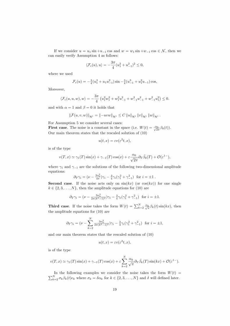
For Assumption 5 we consider several cases:First case. The noise is a constant in the space (i.e. W (t) = α0√

2πβ0(t)).

Our main theorem states that the rescaled solution of (10)

u(t, x) = εv(ε2t, x),

is of the type

v(T, x) ' γ1(T ) sin(x) + γ−1(T ) cos(x) + εα0√2π∂T β0(T ) +O(ε1−),

where γ1 and γ−1 are the solutions of the following two-dimensional amplitudeequations:

∂T γi = (ν − 3α20

4π )γi − 34γi(γ

21 + γ2−1) for i = ±1 .

Second case. If the noise acts only on sin(kx) (or cos(kx)) for one singlek ∈ 2, 3, . . . , N, then the amplitude equations for (10) are

∂T γi = (ν − 3α2k

2π(k2−1)2 )γi − 34γi(γ

21 + γ2−1) for i = ±1.

Third case. If the noise takes the form W (t) =∑Nk=2

αk√πβk(t) sin(kx), then

the amplitude equations for (10) are

∂T γi = (ν −N∑k=2

3α2k

2π(k2−1)2 )γi − 34γi(γ

21 + γ2−1) for i = ±1,

and our main theorem states that the rescaled solution of (10)

u(t, x) = εv(ε2t, x),

is of the type

v(T, x) ' γ1(T ) sin(x) + γ−1(T ) cos(x) + ε

N∑k=2

αk√π∂T βk(T ) sin(kx) +O(ε1−).

In the following examples we consider the noise takes the form W (t) =∑Nk=2 σkβk(t)ek where σk = δαk for k ∈ 2, 3, . . . , N and δ will defined later.

19

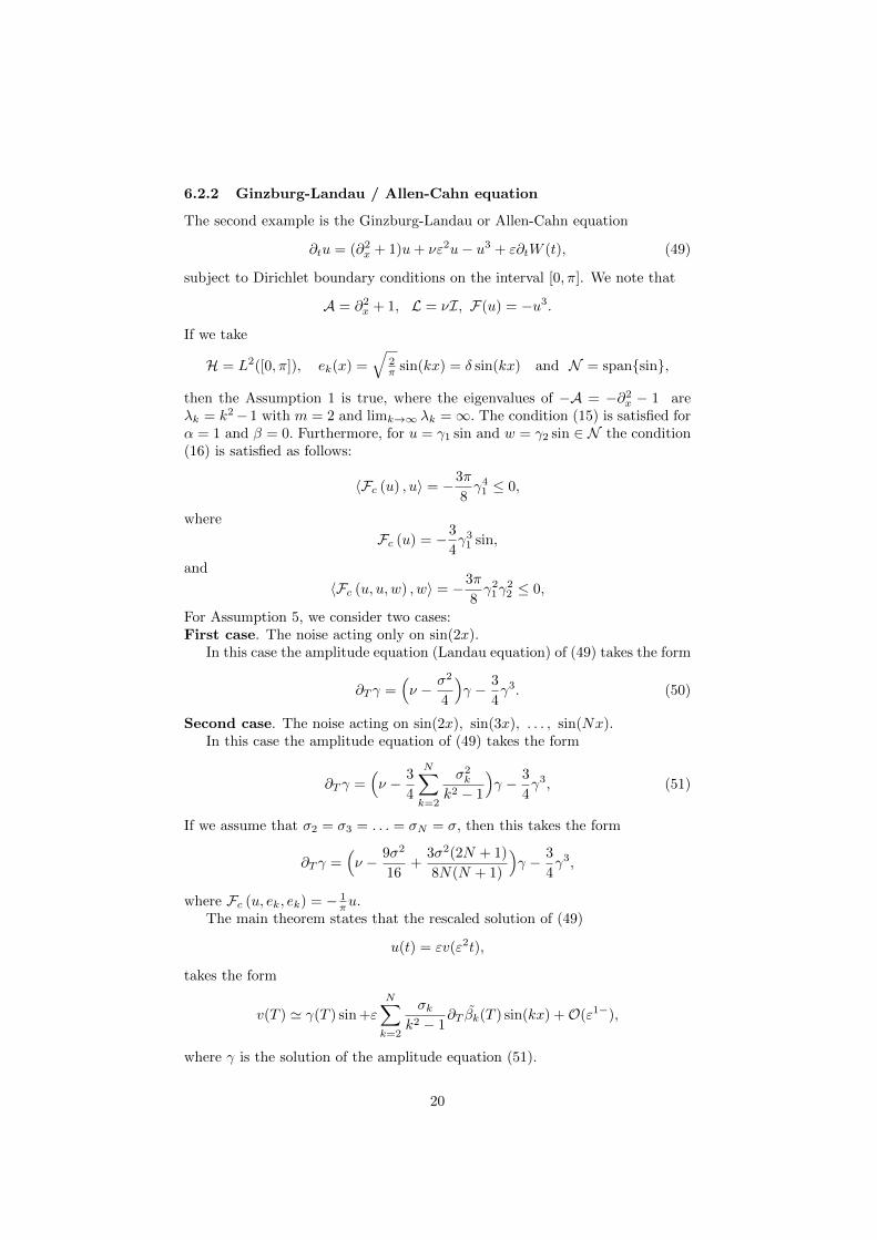
6.2.2 Ginzburg-Landau / Allen-Cahn equation

The second example is the Ginzburg-Landau or Allen-Cahn equation

∂tu = (∂2x + 1)u+ νε2u− u3 + ε∂tW (t), (49)

subject to Dirichlet boundary conditions on the interval [0, π]. We note that

A = ∂2x + 1, L = νI, F(u) = −u3.

If we take

H = L2([0, π]), ek(x) =√

2π sin(kx) = δ sin(kx) and N = spansin,

then the Assumption 1 is true, where the eigenvalues of −A = −∂2x − 1 areλk = k2− 1 with m = 2 and limk→∞ λk =∞. The condition (15) is satisfied forα = 1 and β = 0. Furthermore, for u = γ1 sin and w = γ2 sin ∈ N the condition(16) is satisfied as follows:

〈Fc (u) , u〉 = −3π

8γ41 ≤ 0,

where

Fc (u) = −3

4γ31 sin,

and

〈Fc (u, u, w) , w〉 = −3π

8γ21γ

22 ≤ 0,

For Assumption 5, we consider two cases:First case. The noise acting only on sin(2x).

In this case the amplitude equation (Landau equation) of (49) takes the form

∂T γ =(ν − σ2

4

)γ − 3

4γ3. (50)

Second case. The noise acting on sin(2x), sin(3x), . . . , sin(Nx).In this case the amplitude equation of (49) takes the form

∂T γ =(ν − 3

4

N∑k=2

σ2k

k2 − 1

)γ − 3

4γ3, (51)

If we assume that σ2 = σ3 = . . . = σN = σ, then this takes the form

∂T γ =(ν − 9σ2

16+

3σ2(2N + 1)

8N(N + 1)

)γ − 3

4γ3,

where Fc (u, ek, ek) = − 1πu.

The main theorem states that the rescaled solution of (49)

u(t) = εv(ε2t),

takes the form

v(T ) ' γ(T ) sin +ε

N∑k=2

σkk2 − 1

∂T βk(T ) sin(kx) +O(ε1−),

where γ is the solution of the amplitude equation (51).

20

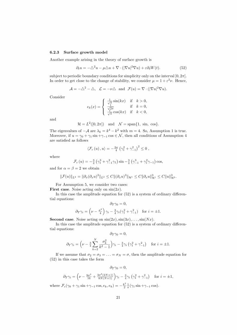
6.2.3 Surface growth model

Another example arising in the theory of surface growth is

∂tu = −42u− µ4u+∇ · (|∇u|2∇u) + ε∂tW (t). (52)

subject to periodic boundary conditions for simplicity only on the interval [0, 2π].In order to get close to the change of stability, we consider µ = 1 + ε2ν. Hence,

A = −42 −4, L = −ν4 and F(u) = ∇ · (|∇u|2∇u).

Consider

ek(x) =

1√π

sin(kx) if k > 0,1√2π

if k = 0,1√π

cos(kx) if k < 0,

andH = L2([0, 2π]) and N = span1, sin, cos.

The eigenvalues of −A are λk = k4 − k2 with m = 4. So, Assumption 1 is true.Moreover, if u = γ0 + γ1 sin +γ−1 cos ∈ N , then all conditions of Assumption 4are satisfied as follows

〈Fc (u) , u〉 = − 3π4

(γ21 + γ2−1

)2 ≤ 0 ,

whereFc (u) = − 3

4

(γ31 + γ2−1γ1

)sin− 3

4

(γ3−1 + γ21γ−1

)cos,

and for α = β = 2 we obtain

‖F(u)‖L2 = ‖∂x(∂xu)3‖L2 ≤ C‖(∂xu)3‖H1 ≤ C‖∂xu‖3H1 ≤ C‖u‖3H2 .

For Assumption 5, we consider two cases:First case. Noise acting only on sin(2x).

In this case the amplitude equation for (52) is a system of ordinary differen-tial equations:

∂T γ0 = 0,

∂T γi =(ν − σ2

4

)γi − 3

4γi(γ21 + γ2−1) for i = ±1.

Second case. Noise acting on sin(2x), sin(3x), . . . , sin(Nx).In this case the amplitude equation for (52) is a system of ordinary differen-

tial equations:∂T γ0 = 0,

∂T γi =(ν − 3

4

N∑k=2

σ2k

k2 − 1

)γi − 3

4γi(γ21 + γ2−1

)for i = ±1.

If we assume that σ2 = σ3 = . . . = σN = σ, then the amplitude equation for(52) in this case takes the form

∂T γ0 = 0,

∂T γi =(ν − 9σ2

16 + 3σ2(2N+1)8N(N+1)

)γi − 3

4γi(γ21 + γ2−1

)for i = ±1,

where Fc(γ0 + γ1 sin +γ−1 cos, ek, ek) = −k2

21π (γ1 sin +γ−1 cos).

21

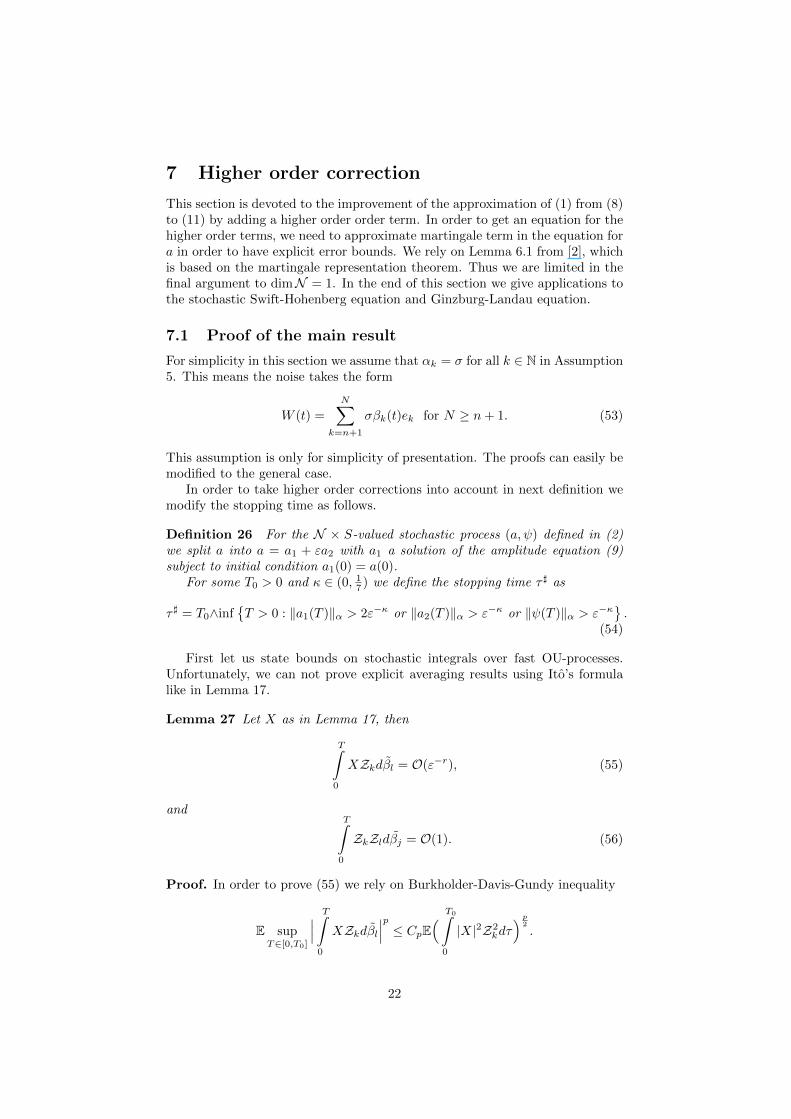
7 Higher order correction

This section is devoted to the improvement of the approximation of (1) from (8)to (11) by adding a higher order order term. In order to get an equation for thehigher order terms, we need to approximate martingale term in the equation fora in order to have explicit error bounds. We rely on Lemma 6.1 from [2], whichis based on the martingale representation theorem. Thus we are limited in thefinal argument to dimN = 1. In the end of this section we give applications tothe stochastic Swift-Hohenberg equation and Ginzburg-Landau equation.

7.1 Proof of the main result

For simplicity in this section we assume that αk = σ for all k ∈ N in Assumption5. This means the noise takes the form

W (t) =

N∑k=n+1

σβk(t)ek for N ≥ n+ 1. (53)

This assumption is only for simplicity of presentation. The proofs can easily bemodified to the general case.

In order to take higher order corrections into account in next definition wemodify the stopping time as follows.

Definition 26 For the N × S-valued stochastic process (a, ψ) defined in (2)we split a into a = a1 + εa2 with a1 a solution of the amplitude equation (9)subject to initial condition a1(0) = a(0).

For some T0 > 0 and κ ∈ (0, 17 ) we define the stopping time τ ] as

τ ] = T0∧infT > 0 : ‖a1(T )‖α > 2ε−κ or ‖a2(T )‖α > ε−κ or ‖ψ(T )‖α > ε−κ

.

(54)

First let us state bounds on stochastic integrals over fast OU-processes.Unfortunately, we can not prove explicit averaging results using Ito’s formulalike in Lemma 17.

Lemma 27 Let X as in Lemma 17, then

T∫0

XZkdβl = O(ε−r), (55)

andT∫

0

ZkZldβj = O(1). (56)

Proof. In order to prove (55) we rely on Burkholder-Davis-Gundy inequality

E supT∈[0,T0]

∣∣∣ T∫0

XZkdβl∣∣∣p ≤ CpE( T0∫

0

|X|2Z2kdτ

) p2

.

22

Using Lemma 17 for some κ0 <12 and Holder inequality, yields

E supT∈[0,T0]

∣∣∣ T∫0

XZkdβl∣∣∣p ≤ CpE

(α2k

2

T0∫0

|X|2dτ +O(ε1−2r−2κ0)) p

2

≤ Cε−pr(

1 + εp2 (1−2κ0)

)≤ Cε−pr.

In order to prove (56) we again use Burkholder-Davis-Gundy inequality to ob-tain

E supT∈[0,T0]

∣∣∣∣∣∣T∫

0

ZkZldβj

∣∣∣∣∣∣p

≤ CpE( T0∫

0

Z2kZ2

l dτ) p

2

. (57)

Using Lemma 17, yields (56). First we prove a technical lemma on ordinary differential equations.

Lemma 28 Let X and Rδ be continuous functions from [0, τ ] to N with X(0) =Rδ(0). If X is a solution of

X(T ) =

∫ T

0

Qa(X)ds+

∫ T

0

Qb(X)ds+Rδ,

where Qa and Qb are linear and bounded operators on N such that

|Qa(X)| ≤ Ca|X|, |Qb(X)| ≤ Cb|X|, (58)

and〈Qb(X), X〉 ≤ 0, (59)

thensup[0,τ ]

|X|2 ≤ [2 + C0(C2a + C2

b )] sup[0,τ ]

|Rδ|2 , (60)

where C0 = 1Ca+1e

2[Ca+1]T0 .

We note that later in the application of this lemma the constant Cb mightgrow with ε while Ca is independent of ε. Therefore condition (59) is importantin order to have no Cb in the exponent.Proof. Define Y = X −Rδ, hence

∂TY = Qa(Y ) +Qa(Rδ) +Qb(Y ) +Qb(Rδ).

Taking the scalar product 〈·, Y 〉 on both sides, we obtain

1

2∂T |Y |2 = 〈Qa(Y ), Y 〉+ 〈Qb(Y ), Y 〉+ 〈Qa(Rδ), Y 〉+ 〈Qb(Rδ), Y 〉 .

Using Cauchy-Schwarz and Young inequalities and (59), yields

∂T |Y |2 ≤ 2[Ca + 1] |Y |2 + [C2a + C2

b ] |Rδ|2 .

23

Applying Gronwall’s lemma, yields for all T ≤ τ

|Y (T )|2 ≤ [C2a + C2

b ]

∫ T

0

|Rδ|2 e2[Ca+1](T−s)ds

≤ C0[C2a + C2

b ] sup[0,τ ]

|Rδ|2 . (61)

To prove (60) we use

|X|2 = |Y +Rδ|2 ≤ 2 |Y |2 + 2 |Rδ|2 ,

and (61). Let us recall Lemma 21 and look closer at the terms of order ε.

Lemma 29 Under Assumptions 1, 3, 4 and 5 with all αk = σ for k ∈ n +1, . . . , N, we obtain

a(T ) = a(0) +

T∫0

Lca(τ)dτ +

T∫0

Fc(a)dτ +

N∑k=n+1

3σ2

2λk

T∫0

Fc(a, ek, ek)dτ

+εMa(T ) + R(T ), (62)

where Ma(T ) is a martingale and it is defined by

Ma(T ) =

∫ T

0

N∑k=n+1

k(a)dβk(s), (63)

where all sums are from n+ 1 to N , if it is not explicitly stated otherwise

k(a) =3σ

λkFc(a, a, ek) +

N∑l=n+1

6σFc(a, ek, el)λk + λl

Zl +

N∑l=n+1

3σ3Fc(ek, el, el)λk(λk + 2λl)

+∑l 6=k

6σFc(ek, ek, el)λl + 2λk

ZkZl +

N∑l=n+1

N∑j=n+1

3σFc(ek, el, ej)λk + λl + λj

ZlZj(64)

andR = R1 +O(ε2−5κ),

where R1 = O(δ2εε2−2κ) is defined in (36).

Proof. In order to obtain (62) we use (34) and use Lemmas 18 and 27.

Lemma 30 Under Assumptions 1, 3, 4 and 5 with all αk = σ, consider somestochastic process ξ = O(ε−r) for r ≥ 0. Then for all p > 0 there exists C > 0such that

E(

supT∈[0,τ]]

|Mξ(T )|p)≤ Cε−2pr, (65)

where Mξ is defined in (63). If ξ is bounded up to time T0, then (65) holds withT0 instead of τ ].

Proof. To prove (65) we take | · |p and expectation after supremum on bothsides of (64) and use Assumptions 4, Lemma 27 and Burkholder-Davis-Gundyinequality.

24

Lemma 31 Under Assumptions 1, 3, 4 and 5 with all αk = σ. If we define aas a = a1 + εa2 such that a1 is a solution of the amplitude equation

da1 = [Lca1 + Fc(a1) +

N∑k=n+1

3σ2

2λkFc(a1, ek, ek)]dT, (66)

then a2 is a solution of

da2 = [Lca2 +3Fc(a1, a1, a2)+

N∑k=n+1

3σ2

2λkFc(a2, ek, ek)]dT +dMa1 +dR2, (67)

where

R2 = ε−1R+ 3ε

∫ T

0

Fc(a1, a2, a2)dτ + ε2∫ T

0

Fc(a2)dτ

+ε

N∑k=n+1

6σ

λk

∫ T

0

Fc(a1, a2, ek)dβk + ε2N∑

k=n+1

3σ

λk

∫ T

0

Fc(a2, a2, ek)dβk

+ε

N∑k=n+1

N∑l=1

6σ

λk + λl

∫ T

0

Fc(a2, ek, el)Zldβk, (68)

withR2 = O(ε1−5κ). (69)

Proof. The equation for a2 is a straightforward calculation using (62) and (66).To bound R2, we take ‖·‖pα on both sides of (68) and use Assumption 4, Lemma27, Burkholder-Davis-Gundy inequality and the definition of τ ] (cf. (54)).

Lemma 32 Under assumptions of Lemma 31. Let a1 be a solution of (66) withinitial condition a1(0) such that |a1(0)| ≤ δε. Define ζ in N as the solution of

dζ = [Lcζ + 3Fc(a1, a1, ζ) +

N∑k=n+1

3σ2

2λkFc(ζ, ek, ek)]dT + dMa1(T ) (70)

with ζ(0) = 0.

If |a1(0)| ≤ δε for some δε ∈ (0, ε−13κ), then for all T0 > 0 and p > 0 there

exist a constant C > 0 such that

supT∈[0,T0]

|a1(T )|p ≤ Cδpε , (71)

andsup

T∈[0,T0]

|ζ(T )| ≤ C(1 + δε) supT∈[0,T0]

|Ma1(T )|. (72)

Proof. The bound on a1 follows directly from Lemma 22.To bound ζ we define

Qa(ζ) = Lcζ +

N∑k=n+1

3σ2

2λkFc(ζ, ek, ek) and Qb(ζ) = 3Fc(a1, a1, ζ),

25

and we obtain from Lemma 28

supT∈[0,T0]

|ζ(T )|2 ≤ [2 + C(1 + δ2ε)] supT∈[0,T0]

|Ma1(T )|2.

Taking the square root on both sides, yields (72).

Remark 33 Note that, from now on, we consider dim(N ) = 1 and identifyN with R using the natural isomorphism γ · e1 7→ γ. Thus for example Fcis defined as 〈F , e1〉 and F2

c is 〈F , e1〉2. Moreover it is easy to check thatthe quadratic variation of Ma1 as a real valued process 〈Ma1 , e1〉 is given by∑Nk=2

∫ T02k(a1)dτ .

Before we prove the main result let us deduce the approximation gk of thequadratic variation function 2

k.Taking the square for both sides of (64) and using Lemma 17, we obtain for

some small κ0 > 0∫ T

0

2k(a1)dτ =

∫ T

0

gk(a1)dτ +O((1 + δ2ε)ε1−4κ0), (73)

where

gk(b1) =9σ2

λ2k[Fc(b1, b1, ek)]2 + θ

(k)1 [Fc(b1, b1, ek)] (74)

+

N∑l=2

18σ4

λl(λk + λl)2[Fc(b1, ek, el)]2 + θ

(k)2 ,

with constants

θ(k)1 =

N∑l=2

9σ4Fc(ek, el, el)λ2kλl

,

and

θ(k)2 =

11σ6F2c (ek)

4λ4k+

N∑l 6=k

9σ6(3λ2k + 4λlλk + 4λ2l )F2c (ek, el, el)

4λ2kλl(λk + 2λl)2

+

N∑l 6=k

9σ6F2c (ek, ek, el)

λkλl(λl + 2λk)2+

N∑l 6=k

N∑j /∈l,k

9σ6F2c (ek, el, ej)

2λlλj(λk + λl + λj)2

+

N∑l 6=k

σ6(6λ2k + 18λl + 3λk)Fc(ek, ek, el)Fc(ek)

2λlλ3k(λk + 2λl)

+

N∑l 6=k

N∑j /∈l,k

9σ6(4λlλj + λ2k + λlλk)Fc(ek, el, el)Fc(ek, ej , ej)4λ2kλlλj(λk + 2λl)(λk + 2λj)

.

Let us state without proof Lemma 6.1 from [2] to bound Ma1(T )− Ma1(T )where the martingale Ma1(T ) is defined in (63) and the martingale Ma1(T ) isdefined in (13).

26

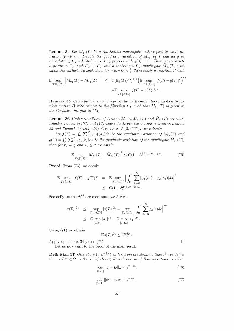
Lemma 34 Let Ma1(T ) be a continuous martingale with respect to some fil-tration (zT )T≥0. Denote the quadratic variation of Ma1 by f and let g bean arbitrary zT -adapted increasing process with g(0) = 0. Then, there existsa filtration zT with zT ⊂ zT and a continuous zT -martingale Ma1(T ) withquadratic variation g such that, for every r0 <

12 there exists a constant C with

E supT∈[0,T0]

∣∣∣Ma1(T )− Ma1(T )∣∣∣p ≤ C(Eg(T0)2p)1/4

(E supT∈[0,T0]

|f(T )− g(T )|p)r0

+E supT∈[0,T0]

|f(T )− g(T )|p/2.

Remark 35 Using the martingale representation theorem, there exists a Brow-nian motion B with respect to the filtration zT such that Ma1(T ) is given asthe stochastic integral in (13).

Lemma 36 Under conditions of Lemma 34, let Ma1(T ) and Ma1(T ) are mar-tingales defined in (63) and (13) where the Brownian motion is given in Lemma

34 and Remark 35 with |a(0)| ≤ δε for δε ∈ (0, ε−13κ), respectively.

Let f(T ) =∫ T0

∑Nk=2

2k(a1)ds be the quadratic variation of Mb1(T ) and

g(T ) =∫ T0

∑Nk=2 gk(a1)ds be the quadratic variation of the martingale Ma1(T ),

then for r0 = 13 and κ0 ≤ κ we obtain

E supT∈[0,T0]

∣∣∣Ma1(T )− Ma1(T )∣∣∣p ≤ C(1 + δ

83pε )ε

13p−

43pκ. (75)

Proof. From (73), we obtain

E supT∈[0,T0]

|f(T )− g(T )|p = E supT∈[0,T0]

∣∣∣ ∫ T

0

N∑k=2

[2k(a1)− gk(a1)]ds

∣∣∣p≤ C(1 + δ2ε)pεp−4pκ0 .

Secondly, as the θ(k)i are constants, we derive

g(T0)2p ≤ supT∈[0,T0]

|g(T )|2p = supT∈[0,T0]

∣∣∣ ∫ T

0

N∑k=2

gk(s)ds∣∣∣2p

≤ C sup[0,T0]

|a1|8p + C sup[0,T0]

|a1|4p .

Using (71) we obtainEg(T0)2p ≤ Cδ8pε .

Applying Lemma 34 yields (75). Let us now turn to the proof of the main result.

Definition 37 Given δε ∈ (0, ε−13κ) with κ from the stopping time τ ], we define

the set Ω∗∗ ⊂ Ω as the set of all ω ∈ Ω such that the following estimates hold:

sup[0,τ]]

‖ψ −Q‖α < ε2−4κ, (76)

sup[0,τ]]

‖ψ‖α < δ0 + ε−12κ , (77)

27

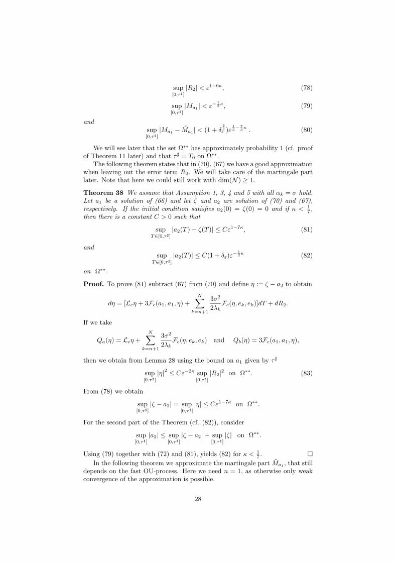
sup[0,τ]]

|R2| < ε1−6κ, (78)

sup[0,τ]]

|Ma1 | < ε−12κ, (79)

andsup[0,τ]]

|Ma1 − Ma1 | < (1 + δ83ε )ε

13−

73κ . (80)

We will see later that the set Ω∗∗ has approximately probability 1 (cf. proofof Theorem 11 later) and that τ ] = T0 on Ω∗∗.

The following theorem states that in (70), (67) we have a good approximationwhen leaving out the error term R2. We will take care of the martingale partlater. Note that here we could still work with dim(N ) ≥ 1.

Theorem 38 We assume that Assumption 1, 3, 4 and 5 with all αk = σ hold.Let a1 be a solution of (66) and let ζ and a2 are solution of (70) and (67),respectively. If the initial condition satisfies a2(0) = ζ(0) = 0 and if κ < 1

7 ,then there is a constant C > 0 such that

supT∈[0,τ]]

|a2(T )− ζ(T )| ≤ Cε1−7κ, (81)

andsup

T∈[0,τ]]|a2(T )| ≤ C(1 + δε)ε

− 12κ (82)

on Ω∗∗.

Proof. To prove (81) subtract (67) from (70) and define η := ζ − a2 to obtain

dη = [Lcη + 3Fc(a1, a1, η) +

N∑k=n+1

3σ2

2λkFc(η, ek, ek)]dT + dR2.

If we take

Qa(η) = Lcη +N∑

k=n+1

3σ2

2λkFc(η, ek, ek) and Qb(η) = 3Fc(a1, a1, η),

then we obtain from Lemma 28 using the bound on a1 given by τ ]

sup[0,τ]]

|η|2 ≤ Cε−2κ sup[0,τ]]

|R2|2 on Ω∗∗. (83)

From (78) we obtain

sup[0,τ]]

|ζ − a2| = sup[0,τ]]

|η| ≤ Cε1−7κ on Ω∗∗.

For the second part of the Theorem (cf. (82)), consider

sup[0,τ]]

|a2| ≤ sup[0,τ]]

|ζ − a2|+ sup[0,τ]]

|ζ| on Ω∗∗.

Using (79) together with (72) and (81), yields (82) for κ < 17 .

In the following theorem we approximate the martingale part Ma1 , that stilldepends on the fast OU-process. Here we need n = 1, as otherwise only weakconvergence of the approximation is possible.

28

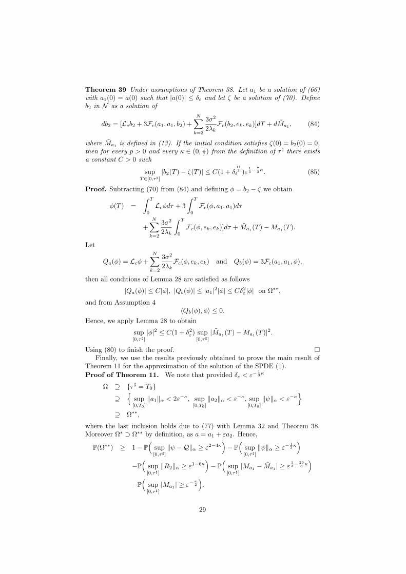
Theorem 39 Under assumptions of Theorem 38. Let a1 be a solution of (66)with a1(0) = a(0) such that |a(0)| ≤ δε and let ζ be a solution of (70). Defineb2 in N as a solution of

db2 = [Lcb2 + 3Fc(a1, a1, b2) +

N∑k=2

3σ2

2λkFc(b2, ek, ek)]dT + dMa1 , (84)

where Ma1 is defined in (13). If the initial condition satisfies ζ(0) = b2(0) = 0,then for every p > 0 and every κ ∈ (0, 17 ) from the definition of τ ] there existsa constant C > 0 such

supT∈[0,τ]]

|b2(T )− ζ(T )| ≤ C(1 + δ113ε )ε

13−

73κ. (85)

Proof. Subtracting (70) from (84) and defining φ = b2 − ζ we obtain

φ(T ) =

∫ T

0

Lcφdτ + 3

∫ T

0

Fc(φ, a1, a1)dτ

+

N∑k=2

3σ2

2λk

∫ T

0

Fc(φ, ek, ek)]dτ + Ma1(T )−Ma1(T ).

Let

Qa(φ) = Lcφ+

N∑k=2

3σ2

2λkFc(φ, ek, ek) and Qb(φ) = 3Fc(a1, a1, φ),

then all conditions of Lemma 28 are satisfied as follows

|Qa(φ)| ≤ C|φ|, |Qb(φ)| ≤ |a1|2|φ| ≤ Cδ2ε |φ| on Ω∗∗,

and from Assumption 4〈Qb(φ), φ〉 ≤ 0.

Hence, we apply Lemma 28 to obtain

sup[0,τ]]

|φ|2 ≤ C(1 + δ2ε) sup[0,τ]]

|Ma1(T )−Ma1(T )|2.

Using (80) to finish the proof. Finally, we use the results previously obtained to prove the main result of

Theorem 11 for the approximation of the solution of the SPDE (1).

Proof of Theorem 11. We note that provided δε < ε−13κ

Ω ⊇ τ ] = T0

⊇

sup[0,T0]

‖a1‖α < 2ε−κ, sup[0,T0]

‖a2‖α < ε−κ, sup[0,T0]

‖ψ‖α < ε−κ

⊇ Ω∗∗,

where the last inclusion holds due to (77) with Lemma 32 and Theorem 38.Moreover Ω∗ ⊃ Ω∗∗ by definition, as a = a1 + εa2. Hence,

P(Ω∗∗) ≥ 1− P(

sup[0,τ]]

‖ψ −Q‖α ≥ ε2−4κ)− P

(sup[0,τ]]

‖ψ‖α ≥ ε−12κ)

−P(

sup[0,τ]]

‖R2‖α ≥ ε1−6κ)− P

(sup[0,τ]]

|Ma1 − Ma1 | ≥ ε13−

293 κ)

−P(

sup[0,τ]]

|Ma1 | ≥ ε−κ2

).

29

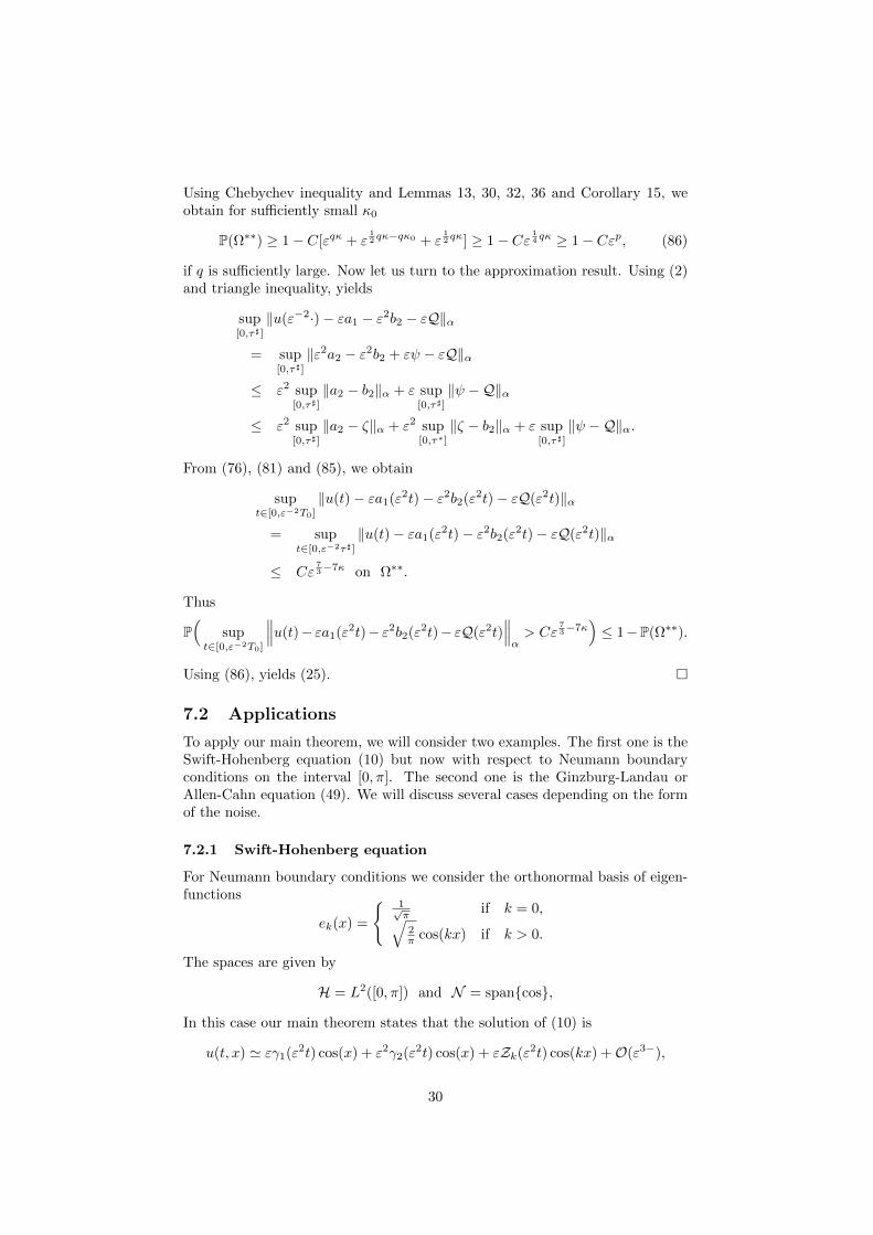
Using Chebychev inequality and Lemmas 13, 30, 32, 36 and Corollary 15, weobtain for sufficiently small κ0

P(Ω∗∗) ≥ 1− C[εqκ + ε12 qκ−qκ0 + ε

12 qκ] ≥ 1− Cε 1

4 qκ ≥ 1− Cεp, (86)

if q is sufficiently large. Now let us turn to the approximation result. Using (2)and triangle inequality, yields

sup[0,τ]]

‖u(ε−2·)− εa1 − ε2b2 − εQ‖α

= sup[0,τ]]

‖ε2a2 − ε2b2 + εψ − εQ‖α

≤ ε2 sup[0,τ]]

‖a2 − b2‖α + ε sup[0,τ]]

‖ψ −Q‖α

≤ ε2 sup[0,τ]]

‖a2 − ζ‖α + ε2 sup[0,τ∗]

‖ζ − b2‖α + ε sup[0,τ]]

‖ψ −Q‖α.

From (76), (81) and (85), we obtain

supt∈[0,ε−2T0]

‖u(t)− εa1(ε2t)− ε2b2(ε2t)− εQ(ε2t)‖α

= supt∈[0,ε−2τ]]

‖u(t)− εa1(ε2t)− ε2b2(ε2t)− εQ(ε2t)‖α

≤ Cε73−7κ on Ω∗∗.

Thus

P(

supt∈[0,ε−2T0]

∥∥∥u(t)− εa1(ε2t)− ε2b2(ε2t)− εQ(ε2t)∥∥∥α> Cε

73−7κ

)≤ 1−P(Ω∗∗).

Using (86), yields (25).

7.2 Applications

To apply our main theorem, we will consider two examples. The first one is theSwift-Hohenberg equation (10) but now with respect to Neumann boundaryconditions on the interval [0, π]. The second one is the Ginzburg-Landau orAllen-Cahn equation (49). We will discuss several cases depending on the formof the noise.

7.2.1 Swift-Hohenberg equation

For Neumann boundary conditions we consider the orthonormal basis of eigen-functions

ek(x) =

1√π

if k = 0,√2π cos(kx) if k > 0.

The spaces are given by

H = L2([0, π]) and N = spancos,

In this case our main theorem states that the solution of (10) is

u(t, x) ' εγ1(ε2t) cos(x) + ε2γ2(ε2t) cos(x) + εZk(ε2t) cos(kx) +O(ε3−),

30

where γ1 and γ2 are the solution of the amplitude equation given below. Wewill discuss three cases depending on the noise.First case. If the noise is a constant in the space, i.e.

W (t) = σβ0(t) ,

then

∂T γ1 =(ν − 3σ2

2

)γ1 −

3

4γ31 ,

and

dγ2 = [(ν − 3σ2

2

)γ2 −

3

4γ21γ2]dT +

3σ2

√2γ1dB.

Second case: If the noise acting on cos(kx) for one k ∈ 2, 4, 5, 6, . . . , N, then

∂T γ1 =(ν − 3σ2

2(k2 − 1)2

)γ1 −

3

4γ31 ,

and

dγ2 = [(ν − 3σ2

2(k2 − 1)2

)γ2 −

3

4γ21γ2]dT +

3σ2

2√

2(k2 − 1)3γ1dB.

Third case: If the noise takes the form

W (t) = σβ3(t) cos(3x) ,

then

∂T γ1 =(ν − 3σ2

128

)γ1 −

3

4γ31 ,

and

dγ2 = [(ν − 3σ2

128

)γ2 −

3

4γ21γ2]dT +

3σ

256γ1

√(γ21 +

σ2

32)dB.

7.2.2 Ginzburg-Landau / Allen-Cahn equation

Our main theorem states that the solution of (49) takes the form

u(t, x) ' εγ1(ε2t) sin(x) + ε2γ2(ε2t) sin(x) + εZk(ε2t) sin(kx) +O(ε3−),

where γ1 and γ2 are the solution of the amplitude equations given below. Wewill discuss three cases depending on the noise.First case. Noise acting on sin(kx) for one k ∈ 2, 4, 5, 6, . . . , N. In this case

∂T γ1 =(ν − 3σ2

4(k2 − 1)

)γ1 −

3

4γ31 ,

and

dγ2 = [(ν − 3σ2

4(k2 − 1)

)γ2 −

3

4γ21γ2]dT +

3σ2

2√

2(k2 − 1)3γ1dB.

Second case. Noise acting only on sin(3x). In this case

∂T γ1 =(ν − 3σ2

32

)γ1 −

3

4γ31 ,

31

and

dγ2 = [(ν − 3σ2

32

)γ2 −

3

4γ21γ2]dT +

3σ

32γ1

√(γ21 +

σ2

16)dB.

Third case. The noise is of the form

W (t) =

3∑k=2

σβk(t)ek .

In this case

∂T γ1 =(ν − 11σ2

32

)γ1 −

3

4γ31 ,

and

dγ2 = [(ν − 11σ2

32

)γ2 −

3

4γ21γ2]dT + dM,

where

dM =3σ

32

(γ41 +

1289σ2

128γ21 +

89σ4

147

)1/2

dB.

Acknowledgements

This work is supported by the Deutsche Forschungsgemeinschaft (DFG BL535/9-1), and Wael Mohammed is supported by a fellowship from the Egyptian gov-ernment in the Long Term Mission system.

References

[1] D. Blomker. Amplitude equations for stochastic partial differential equa-tions. Interdisciplinary mathematical sciences-Vol. 3, World Scientific(2007).

[2] D. Blomker, M. Hairer, and G.A. Pavliotis. Multiscale analysis for stochas-tic partial differential equations with quadratic nonlinearities. Nonlinearity,20:1–25 (2007).

[3] M.C. Cross and P.C. Hohenberg. Pattern formation outside of equilibrium.Rev. Mod. Phys., 65:581–1112, (1993).

[4] A. Hutt, A. Longtin, L. Schimansky-Geier. Additive global noise delaysTuring bifurcations. Phys. Rev. Lett., 98:230601, (2007).

[5] A.Hutt, A.Longtin, L.Schimansky-Geier. Additive noise-induced Turingtransitions in spatial systems with application to neural fields and theSwift-Hohenberg equation. Physica D, 237:755–773, (2008).

[6] A.Hutt. Additive noise may change the stability of nonlinear systems. Eu-rophys. Lett. 84(3):34003, (2008).

[7] P. C. Hohenberg and J. B. Swift. Effects of additive noise at the onset ofRayleigh-Benard convection, Physical Review A, 46:4773–4785, (1992).

32

[8] Z.-W. Lai and S. Das Sarma. Kinetic growth with surface relaxation: Con-tinuum versus atomistic models Phys. Rev. Lett. 66:2348–2351, (1991)

[9] C. Liu. A fourth-order parabolic equation in two space dimensions. Math.Methods Appl. Sci. 30(15):1913–1930, (2007).

[10] A.J. Roberts. A step towards holistic discretisation of stochastic partialdifferential equations. ANZIAM J., 45(E):C1–C15, (2003).

[11] A. J. Roberts, Wei Wang. Macroscopic reduction for stochastic reaction-diffusion equations. Preprint, 2008, arXiv:0812.1837v1 [math-ph]

33