Indag. Mathem., N.S., 8 (4). 471-492

On cubic-linear polynomial mappings

December 22,1997

by Gianluca Gorni and Gaetano Zampieri

Universitd di Udine, Dipartimento di Matematica e Informatica, via delle Scienze 208,

33100 Udine, Italy,

e-mail: gorni@dimi.uniud.it

Dipartimento di Matematica, via Carlo Albert0 IO, 10123 Torino, Italy,

e-mail: zampieri@dm.unito.it

Communicated by Prof. T.A. Springer at the meeting of November 25,1996

ABSTRACT

In the field of the Jacobian conjecture it is well-known after Druikowski that from a polynomial ‘cubic-homogeneous’ mapping we can build a higher-dimensional ‘cubic-linear’ mapping and the other way round, so that one of them is invertible if and only if the other one is. We make this point clearer through the concept of ‘pairing’ and apply it to the related conjugability problem: one of the two maps is conjugable if and only if the other one is; moreover, we find simple formulas expressing the inverse or the conjugations of one in terms of the inverse or conjugations of the other. Two nontrivial examples of conjugable cubic-linear mappings are provided as an application.

I. INTRODUCTION

The following conjecture was essentially originated by Keller [14] in 1939:

Jacobian Conjecture. For all n E N, if f : @” + C” has polynomial compo- nents and the Jacobian determinant detf’( ) . x IS a nonzero constant throughout C”, thenf is a polynomial automorphism of @“, that is, a bijective polynomial map with polynomial inverse.

There is a huge literature on this topic and also some wrong proofs were pub- lished. A basic paper on the subject is [2] by Bass, Connell and Wright. The re- cent proceedings of conference [IO], and in particular its first paper, by the editor van den Essen, are a good update on this research field, rich in questions of different nature.

In everything that follows R or R” can be substituted for @ and @” with only

471

trifling adjustments. Before proceeding it is convenient to establish some no- tations first: if x,y E C” we will write x * y for the componentwise product of the two vectors: x * y := (xi yi , x2 ~2, . . . ,x,, yn) E C”. The powers with respect to this multiplication will be denoted by x* 2, x* 3, . . The symbol Z,, will be identity mapping (or matrix) in C ‘. The minus signs in formulas (1.1) and (1.2) below may seem odd but will later simplify some expressions in Section 4.

Definition 1.1. A mappingf : @” + C” will be called ‘cubic-homogeneous’ if there exists a trilinear symmetric function g : @” x @” x C” + @” such that

(1.1) f(x) =x--(x,x,x) forallxEc=“,

It will be called ‘cubic-linear’ if there exists an n x n matrix A such that

(1.2) f(x) = x - (Ax)*~ for all x E C”.

Cubic-homogeneous and cubic-linear mappings with constant Jacobian de- terminant will be called ‘Yagzhev maps’ and ‘Druikowski maps’ respectively.

Two classical ‘reduction’ results bear in particular on the present paper. They restrict the class of polynomial functions over which it is sufficient to con- centrate the attention in order to prove or disprove the full conjecture: the first reduction was to Yagzhev maps (Yagzhev [18] and independently Bass-Con- nell-Wright [2]) and the second was to the smaller class of the Druikowski maps (Druikowski [7]).

A side issue of the Jacobian conjecture was introduced in [5]: given a pa- rameter X E UZ\{O, 1) and a polynomial mapping f : C” -+ C” such that f(0) = O,f’(O) = Z,, the problem is to find a global analytic conjugation, i.e., an invertible analytic function kx : C” -+ @” such that the following diagram

commutes:

and with again the ‘normalizing’conditions kx(O) = 0, k;(O) = I,,. We will also be handling functions kx that are like conjugation, except for either being de- fined only on a neighbourhood of 0 E C” or for possibly failing to be invertible: these will be called pre-conjugations.

If a mappingf : @” -+ C” admits a conjugation for some X, then the discrete dynamical system of the backward and forward iterates of Xf is ‘trivial’. In particular, f is invertible, and this observation was in fact the original motiva- tion for raising the problem. There was some hope to prove that the Jacobian conjecture was true by proving first that all polynomial maps in a suitable class are conjugable.

With the work that has been done in the past few years on conjugations, and

472

specially after the examples found by A. van den Essen and E. Hubbers, the hope to possibly prove the Jacobian conjecture through conjugations has dim- med, although we cannot rule it out yet. What is still very well possible is that a counterexample to the Jacobian conjecture may be found as a by-product of research in conjugability. One unexpected and encouraging by-product, in a seemingly unrelated area, is already here: it is a very simple and elegant coun- terexample to Markus-Yamabe conjecture in dimension 2 3, due to A. Cima, A. van den Essen, A. Gasull, E. Hubbers and F. Mafiosas [4].

The state of the art in the conjugation business is as follows. There are nor- malized polynomial automorphisms that are not conjugable: the earliest one was given in [ll], and it is of ‘quintic-homogeneous’ form, but we have later realized that also the old and well-known map in two dimensions

(1.4) f : ; H 0 (

x+I(::$)2)

is a counterexample (three fixed points for Xf outside the origin are quickly found when X E C\{O, 1)). We do not know yet if all Yagzhev maps are nec- essarily conjugable, although a theorem in [12] seems to make it hard to find counterexamples. Yagzhev maps have been given for which global conjugations exist that are analytic but not polynomial themselves ([lo, page 2311 and [12]). These last examples have in turn taught us a lesson on the Jacobian conjecture, namely, on the structure of the local inverse of Yagzhev maps (see [ 131).

The present paper was born out of the effort to find whether a particular Druikowski mapping (Example 6.1 below) was conjugable. We have discovered that there is a strong link between the conjugability of a Druikowski map, or, more generally, of a cubic-linear map F, and the conjugability of a certain lower-dimensional cubic-homogeneous map f. The exact relation between F

and f is described as follows:

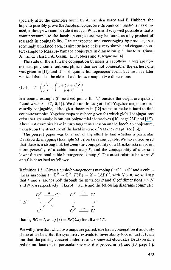
Definition 1.2. Given a cubic-homogeneous mapping f : C" 4 C" and a cubic- linear mapping F : cN -+ cN, F(X) := X - (AX)*3, with N > n, we will say that f and F are ‘paired’ through the matrices B and C (of dimensions n x N

and N x n respectively) if ker A = ker B and the following diagrams commute:

that is, BC = I, and f (x) = BF(Cx) for all x E C”.

We will prove that when two maps are paired, one has a conjugation if and only if the other has. But the symmetry extends to invertibility too: in fact it turns out that the pairing concept underlies and somewhat elucidates Druikowski’s reduction theorem, in particular the way it is proved in [9], and [lo, page 1 I].

473

The main results of this paper can be summed up in the following theorem,

which shows that the problems of both invertibility and conjugation have the

same answers if two maps are paired.

Theorem 1.3. Every cubic-homogeneous map can bepaired to a cubic-linear map and vice versa. Moreover, tff and F arepaired, each of thefollowingpropertiesfor one of the two mappings implies the same property for the other, for a given

x E @ \{O}, 1x1 # 1 : 1. one-to-one,

2. onto. 3. invertible with polynomial inverse, 4. constant Jacobian determinant, 5. existence of a globalpre-conjugation. 6. the globalpre-conjugation is onto, 7. the globalpre-conjugation is one-to-one, 8. the globalpre-conjugation is a polynomial map, 9. the conjugation has a polynomial inverse.

The existence of global pre-conjugations is guaranteed when 1x1 > 1, and also when f and F are invertible.

Here is an assortment of formulas connecting F, f and the respective (globally

defined) pre-conjugations & , kx , that are true for all x, y E C”, X, Y E CN,

whenever every single piece just makes sense:

(1.6)

f (BX) = BF(X), detf’(x) = det F’(Cx), det F’(X) = detf’(BX),

f-‘(y) =BF-‘(Cy), F-‘(Y) = Y - F(Cf -‘(BY)) + Cf -‘(BY),

kx (x) = BKA (Cx), kx (BX) = BKA (X),

k,‘(y)=BK,-‘(Cy), K,-‘(Y)= Y-&(Ck,‘(BY))+Ck,‘(BY).

The first two rows (and in particular the formula for F-l in terms off -I) were

somehow implicit in the treatment of [9] and [lo, page II], but they were hidden

beneath layers of changes of variables.

The rest of the paper is organized as follows. Section 2 concerns the existence

of pairing and some basic properties. Section 3 is about invertibility. Section 4

is an introduction to pre-conjugations, in the simpler cubic-homogeneous set-

ting and with a much easier proof than in [5], and not relying on Poincart’s

theorem [l, Sec. 251 either. Section 5 shows how pairing behaves under con-

jugation. Section 6 illustrates two examples: the first is Druikowski’s ex-

ample 7.8 from [9] in dimension 15, which turns out to be conjugable through a

polynomial automorphism; in the end we compute a Druikowski pairing to

van den Essen’s example from [lo, page 2311, thus producing a new Druikowski

map in dimension 16 for which global analytic conjugations exist which are not

polynomial.

474

2. PAIRING A CUBIC-HOMOGENEOUS MAPPING TO A CUBIC-LINEAR ONE,

AND VICE VERSA

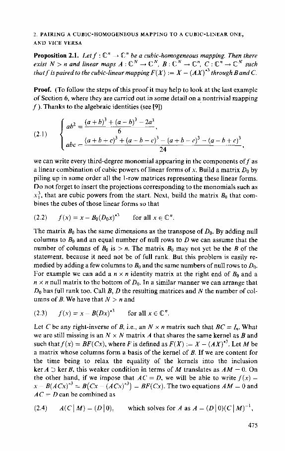
Proposition 2.1. Letf : @” 4 C” be a cubic-homogeneous mapping. Then there exist N > n and linear maps A : CN 4 CN, B : UIN + C”, C : @” -+ IIN such

thatf ispaired to the cubic-linear mapping F(X) := X - (AX)*3 through Band C.

Proof. (To follow the steps of this proof it may help to look at the last example of Section 6, where they are carried out in some detail on a, nontrivial mapping f). Thanks to the algebraic identities (see [9])

(2.1)

ab2 = (a + b)3 + (a - b)3 - 2a3 7 6

abc = (a + b + c)~ + (a - b - c)~ - (a + b - c)~ - (a - b + c)~

24 7

we can write every third-degree monomial appearing in the components off as a linear combination of cubic powers of linear forms of x. Build a matrix DO by piling up in some order all the l-row matrices representing these linear forms. Do not forget to insert the projections corresponding to the monomials such as x:, that are cubic powers from the start. Next, build the matrix BO that com- bines the cubes of those linear forms so that

(2.2) f(x) = x - Bo(Dox) *3 for all x E @”

The matrix BO has the same dimensions as the transpose of DO. By adding null columns to BO and an equal number of null rows to D we can assume that the number of columns of BO is > n. The matrix BO may not yet be the B of the statement, because it need not be of full rank. But this problem is easily re- medied by adding a few columns to BO and the same numbers of null rows to DO. For example we can add a n x n identity matrix at the right end of B. and a n x n null matrix to the bottom of DO. In a similar manner we can arrange that DO has full rank too. Call B, D the resulting matrices and N the number of col- umns of B. We have that N > n and

(2.3) f(x) = x - B(Dx)*3 for all x E C”.

Let C be any right-inverse of B, i.e., an N x n matrix such that BC = Z,,. What we are still missing is an N x N matrix A that shares the same kernel as B and such thatf(x) = BF(Cx), where F is defined as F(X) := X - (AX)*3. Let M be a matrix whose columns form a basis of the kernel of B. If we are content for the time being to relax the equality of the kernels into the inclusion ker A II ker B, this weaker condition in terms of M translates as AA4 = 0. On the other hand, if we impose that AC = D, we will be able to write f(x) = x - B(ACX)*~ = B(Cx - (ACX)“~) = BF(Cx). The two equations AM = 0 and AC = D can be combined as

(2.4) A(CIM) = (DIO), whichsolvesforAasA=(DIO)(C(M)-‘,

475

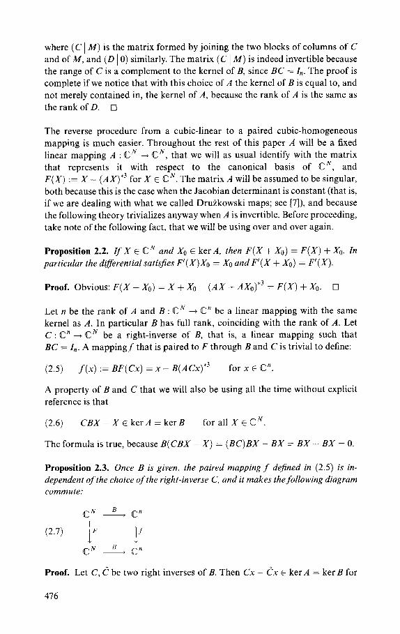
where (C 1 M) is the matrix formed by joining the two blocks of columns of C and of M, and (D IO) similarly. The matrix (C 1 M) is indeed invertible because the range of C is a complement to the kernel of B, since BC = Z,,. The proof is complete if we notice that with this choice of A the kernel of B is equal to, and not merely contained in, the kernel of A, because the rank of A is the same as the rank of D. •I

The reverse procedure from a cubic-linear to a paired cubic-homogeneous mapping is much easier. Throughout the rest of this paper A will be a fixed linear mapping A : CN -9 CN, that we will as usual identify with the matrix that represents it with respect to the canonical basis of cN, and F(X) := X - (AX)*3 for X E Q=‘. The matrix A will be assumed to be singular, both because this is the case when the Jacobian determinant is constant (that is, if we are dealing with what we called Druikowski maps; see [7]), and because the following theory trivializes anyway when A is invertible. Before proceeding, take note of the following fact, that we will be using over and over again.

Proposition 2.2. Zf X E cN and Xe E ker A, then F(X + X0) = F(X) + X0. In

particular the d~j%rential satisfies F’(X)Xo = X0 and F’(X + X0) = F’(X).

Proof. Obvious: F(X + X0) = X + Xo - (AX + AXO)*~ = F(X) + Xo. q

LetnbetherankofAandB:CN --f @” be a linear mapping with the same kernel as A. In particular B has full rank, coinciding with the rank of A. Let C : C” + CN be a right-inverse of B, that is, a linear mapping such that BC = Z,. A mappingf that is paired to F through B and C is trivial to define:

(2.5) S(x) := BF(Cx) = x - B(ACX)*~ for x E @‘I.

A property of B and C that we will also be using all the time without explicit reference is that

(2.6) CBX-X~kerA=kerB for all X E cN.

The formula is true, because B( CBX - X) = (BC) BX - BX = BX - BX = 0.

Proposition 2.3. Once B is given, the paired mapping f defined in (2.5) is in-

dependent of the choice of the right-inverse C, and it makes thefollowing diagram

commute:

Proof. Let C, d be two right inverses of B. Then CX - Cx E ker A = ker B for

476

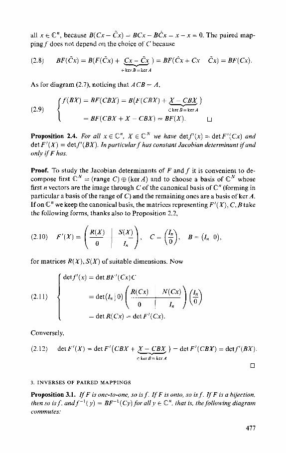
all x E @“, because B(Cx - cx) = BCx - BCx = x - x = 0. The paired map- ping f does not depend on the choice of C because

(2.8) BF(Cx) = B(F(Cx) + @$x ) = BF(& + Cx - cx) = BF(Cx).

EkerB=kerA

As for diagram (2.7), noticing that ACB = A,

(2.9)

f (BX) = BF(CBX) = B(F(CBX) + ,x -FB$ )

ekerE=kerA

= BF(CBX + X - CBX) = BF(X). 0

Proposition 2.4. For all x E Cc”, X E @‘@ we have detf(x) = det F’(Cx) and

det F’(X) = detf (BX). In particular f has constant Jacobian determinant ifand

only if F has.

Proof. To study the Jacobian determinants of F andf it is convenient to de- compose first CN = (range C) @ (ker A) and to choose a basis of CN whose first n vectors are the image through C of the canonical basis of @” (forming in particular a basis of the range of C) and the remaining ones are a basis of ker A.

If on C” we keep the canonical basis, the matrices representing F’(X), C, B take the following forms, thanks also to Proposition 2.2,

(2.10) F’(X) = (w), C= ($ B= (InlO),

for matrices R(X), S(X) of suitable dimensions. Now

[ detf’(x) = det BF’(Cx)C

I = detR(Cx) = detF’(Cx).

Conversely.

(2.12) detF’(X) =detF’(CBX+F-_CBT) =detF’(CBX) =detf’(BX).

ckerB=kerA

cl

3. INVERSES OF PAIRED MAPPINGS

Proposition 3.1. If F is one-to-one, so is f. If F is onto, so is f. If F is a bijection,

then so is f, andf -’ ( y) = BF-’ (Cy) for ally E a=“. that is, the following diagram

commutes:

477

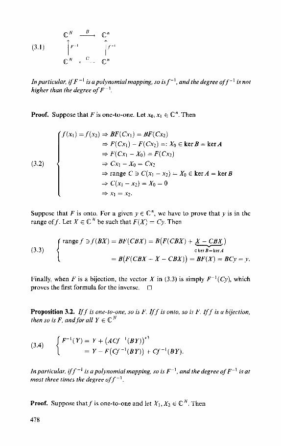
In particular, ifF-’ is apolynomialmapping, so isf-‘, and the degree off-’ isnot

higher than the degree of F-l.

Proof. Suppose that F is one-to-one. Let x0, XI E @“. Then

(3.2)

‘f (x,) = f (xl) =+ BF(Cx,) = BF(Cx2)

+ F(Cxl) - F(Cx2) =: X0 E ker B = kerA

+ F(Cx, - X0) = F(Cx2)

=+ CXl - x0 = cx2

+ range C 3 C(xt - x2) = X0 E ker A = ker B

=+ C(x, - x2) = X0 = 0

=+-Xl =x2.

Suppose that F is onto. For a given y E C”, we have to prove that y is in the range off. Let X E CN be such that F(X) = Cy. Then

(3.3)

range f 3 f (BX) = BF(CBX) = B(F(CBX) + ,X -F&X)

ckerB=kerA

= B(F(CBX + X - CBX)) = BF(X) = BCy = y.

Finally, when F is a bijection, the vector X in (3.3) is simply F;-‘(Cy), which proves the first formula for the inverse. q

Proposition 3.2. Iff is one-to-one, so is F. Iff is onto, so is F. Zff is a bijection,

then so is F, andfor all Y E C N

(3.4) F-‘(Y) = Y + (ACf-‘(BY))”

= Y - F(Cf -‘(BY)) + Cf -‘(BY).

In particular, iff -’ is a polynomial mapping, so is F-‘, and the degree of F-’ is at

most three times the degree off -I.

Proof. Suppose that f is one-to-one and let XI, X2 E UZN. Then

478

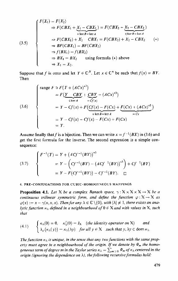
(3.5)

F(Xl) = W2)

=+ F(CBX~ +F -“cm) = F(CBX2 +,x2 -“cB&)

ckerB=kerA l kerB=kerA

=+ F(CBX~) + x1 - CBX~ = F(CBX2) +x2 - csx2 (*)

* BF( CBX~ ) = BF( CBX2)

*fW1) =f(BX2)

=+ BXI = BX2 using formula (*) above

*X1 =X2.

Suppose that f is onto and let Y E CN. Let x E C” be such that f(x) = BY.

Then

’ range F 3 F( Y + (ACx)*3)

= F(D + w + (ACX)‘~)

EkerA = Cf (x)

(3.6) = Y - Cf(x) + F(cf(x) - F(Cx) +F(Cx) +_(ACx)*:) ,

ckerB=kerA = cx

= Y - Cf(x) + C’(x) - F(Cx) + F(Cx)

= Y.

Assume finally thatf is a bijection. Then we can write x =f-‘(BX) in (3.6) and get the first formula for the inverse. The second expression is a simple con- sequence:

(3.7)

F-‘(Y) = Y + (ACf-‘(BY))*3

= Y - (Cf-‘(BY) - (ACf-1(BY))‘3) + Cf-‘(BY)

= Y - F(Cf-‘(BY)) + Cf-‘(BY). 0

4. PRE-CONJUGATIONS FOR CUBIC-HOMOGENEOUS MAPPINGS

Proposition 4.1. Let M be a complex Banach space, y : X x X x X + X be a

continuous trilinear symmetric form, and dejne the function p : X + X as

p(x) := x - y(x, x, x). Then for any X E @ \{O}, with 1x1 # 1, there exists an ana-

lytic function 6~ defined in a neighbourhood of 0 E M and with values in X, such

that

(4.1) m(O) = 0, n;(O) = Zx (the identity operator on X) and

X,(nx(y)) = nx(AY) f or all y E M such that y, Ay E dom K.X.

The function nx is unique, in the sense that any two functions with the sameprop-

erty must agree in a neighbourhood of the origin. Zf we denote by P,,, the homo-

geneous term of degree m in the Taylor series ICY = C, > 0 P,,, of nA centered in the

origin (ignoring the dependence on A), the following recursive formulas hold:

479

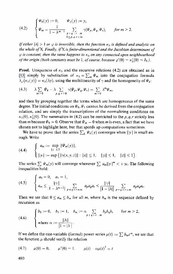
@O(Y) := 0, 91 (Y) := Y,

(4.4 P, = 1

1 - AM-1 C y(pPp, @,, pir), form 2 2. p+g+r=m OiP?Y,r<m

If either 1x1 > 1 or ‘p is invertible, then the function KA is defined and analytic on the whole of X Finally, ifW is$nite-dimensional and the Jacobian determinant of ‘p is constant, then the same happens to KA on any connected open neighbourhood

of the origin (both constants must be 1, of course, because p’(O) = n;(O) = IX).

Proof. Uniqueness of rig and the recursive relations (4.2) are obtained as in [13] simply by substitution of h;,, = C, 9, into the conjugation formula

X&A(Y)) = Q(X v , using the multilinearity of y and the homogeneity of pk: 1

(4.3) xc @k-x c y(lTi,,!&&) = c AM@,, m>O P\%‘>O m>O

and then by grouping together the terms which are homogeneous of the same degree. The initial conditions on PO, !Pi cannot be derived from the conjugation relation, and are simply the transcriptions of the normalizing conditions on KA(O), K;(O). The summation in (4.2) can be restricted to the p, q, r strictly less than m because !Po = 0. Observe that !Pm = 0 when m is even, a fact that we have chosen not to highlight here, but that speeds up computations sometimes.

We have to prove that the series xk @k(Y) converges when ]I yll is small en- ough. Write

(4.4)

1

~~ := ,I;;:, Il@dY)Il,

IIYII := suP{llr(%YAI : llxll I: 1, IIYII I 1,

The series C Pm(y) will converge whenever C a,]] ~11”’ inequalities hold:

( uo = 0, ai = 1,

llzll I I>.

< +ca The following

(4.5) \

llrll llrll avz < 11 - A”-‘1 p+qg;w, u~“qur 5 p - lpj p+q+r=m

c apaqar.

Then we see that 0 5 a,,, 5 b, for all m, where b, is the sequence defined by recursion as

(4.6)

bo:=O, bl:=l, b,:=a c bPW for m > 2, p+q+r=m

IIXII where (Y := ~ 11 - ILlI

If we define the one-variable (formal) power series p(t) := C b,t”, we see that the function p should verify the relation

(4.7) P(0) = 0, P’(0) = 1, p(t) - ap(t)3 = t

480

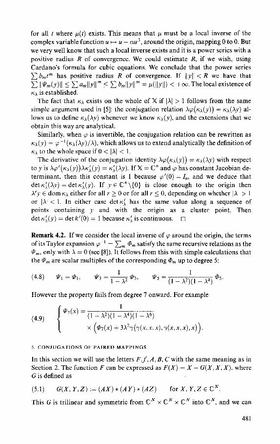
for all t where p(t) exists. This means that p must be a local inverse of the complex variable function u H u - ou3, around the origin, mapping 0 to 0. But we very well know that such a local inverse exists and it is a power series with a

positive radius R of convergence. We could estimate R, if we wish, using Cardano’s formula for cubic equations. We conclude that the power series

C b,t”’ has positive radius R of convergence. If ]lvll < R we have that

C IIPm(~)]I 2 CU~]~_V]]~ I Cbnlllyllnl = p(l/yll) < +cc.Thelocalexistenceof no is established.

The fact that r;x exists on the whole of X if 1x1 > 1 follows from the same simple argument used in [S]: the conjugation relation Xcp(~,x(~)) = KA(AY) al- lows us to define ox whenever we know &x(y), and the extensions that we obtain this way are analytical.

Similarly, when cp is invertible, the conjugation relation can be rewritten as K;X(Y) = cp-‘(KA(A~)/X), which allows us to extend analytically the definition of K,, to the whole space if 0 < IX] < 1.

The derivative of the conjugation identity Xcp(lc~(y)) = ox with respect to ~‘is Xcp’(~x(y))X~L(y) = KA(AY). If M = C” and cp has constant Jacobian de- terminant, then this constant is 1 because ~‘(0) = Z,,, and we deduce that det r;A(Aq’) = det K;(y). If y E C” \{O} is close enough to the origin then X’y E dom K.X either for all r > 0 or for all r 5 0, depending on whether 1x1 > 1 or 1x1 < 1. In either case det K; has the same value along a sequence of points containing _V and with the origin as a cluster point. Then det K.~(Y) = det k’(0) = 1 because K; is continuous. q

Remark 4.2. If we consider the local inverse of ‘p around the origin, the terms of its Taylor expansion ‘p-i = C, Qrn satisfy the same recursive relations as the 9,, only with X = 0 (see [S]). It follows from this with simple calculations that the !Pm are scalar multiples of the corresponding Qrn up to degree 5:

(4.8) Pl = @l, 1

*3 =- 1 - x2 @3, p5 = (1 _ x’;(l _ X4) @5.

However the property fails from degree 7 onward. For example

(4.9) 97(x) = (1 _ x2)(1 :x4)(1 _ ~6)

x @7(x) + 3X27(7( x,x.x~,Y(xJ~x,.x)).

5. CONJUGATIONS OF PAIRED MAPPINGS

In this section we will use the letters F,f, A, B, C with the same meaning as in Section 2. The function F can be expressed as F(X) = X - G(X, X, X), where G is defined as

(5.1) G(X, Y,Z) := (AX) * (A Y) * (AZ) for X, Y,Z E CN.

This G is trilinear and symmetric from CN x CN x CN into CN, and we can

481

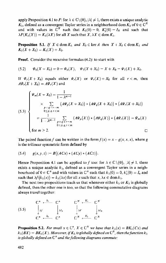
apply Proposition 4.1 to F: for X E C\(O), 1x1 # 1, there exists a unique analytic KA, defined as a convergent Taylor series in a neighborhood dom Kx of 0 E CN and with values in CN such that Kx(O) = 0, K,‘(O) = IN and such that XF(Kx(X)) = Kx(XX) for all X such that X, XX E dom Kx.

Proposition 5.1. Zf X E dom KA and X0 E ker A then X + X0 E dom KA and

Kx(X + Xo) = Kx(X) + Xo.

Proof. Consider the recursive formulas (4.2): to start with

(54 !&)(x+&)=0=!&(x), s,(x+xo)=~+~o=~l(~)+~o.

If p,(X + X0) equals either 9,.(X) or Gr(X) +X0 for all r < m, then A@,(X + X0) = M&Y) and

(5.3)

x c (A@p(X + X0)) * (A@,@- + X0)) * (A&(X + X0)) p+q+r=m O~P,q,r<~

1 c = 1 - A”-’ p+q+r=m (A@P(W) * (A@qW)) * (AWW) = @m(-u

O<p,q,r<m

for m > 2. 0

The paired functionf can be written in the formf(x) = x - g(x, x, x), where g is the trilinear symmetric form defined by

(5.4) g(x,y,z) := B((ACx) * (ACy) * (ACZ)).

Hence Proposition 4.1 can be applied to f too: for X E @ \{O}, 1x1 # 1, there exists a unique analytic kx, defined as a convergent Taylor series in a neigh- bourhood of 0 E C” and with values in @” such that kx(O) = 0, k:(O) = Z,, and such that Af (kx(x)) = kx(Xx) for all x such that x, Xx E dom kx.

The next two propositions teach us that whenever either kx or KA is globally defined, then the other one is too, so that the following commutative diagrams always travel together:

Proposition 5.2. For small x E C”, X E CN we have that kx(x) = BKx(Cx) and kx (BX) = BKx (X). Moreover, if Kx is globally dejined on CN, then the function kx is globally defined on @” and the following diagrams commute:

482

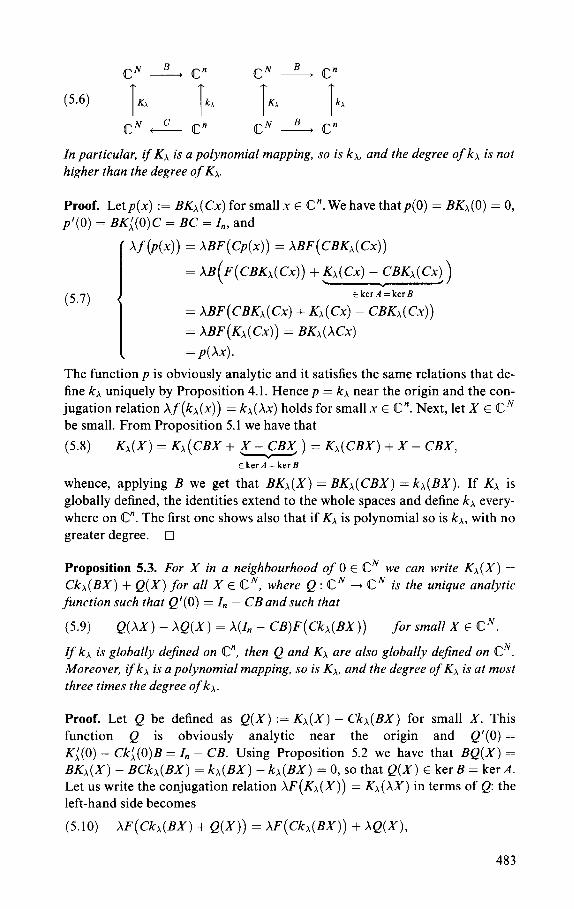
(5.6) Tf+ TkA ‘r:l- ) CN A @” cN B @”

In particular, if Kx is a polynomial mapping, so is kx. and the degree of kx is not higher than the degree of Kx.

Proof. Letp(x) := BKx(Cx) for small x E C”. We have thatp(0) = BKx(0) = 0, p’(0) = BKi(O)C = BC = Z,, and

/ Xf (P(x)) = XBF(Cp(x)) = XBF(CBKA(Cx))

= XB(F(CBKx(Cx)) + Kx(Cx) - CBKx(Cx)) . 2

(5.7) < ckerA=kerB

= XBF(CBKA(Cx) + Kx(Cx) - CBKx(Cx))

= XBF(KA(Cx)) = BKA(XCx)

\ = p(Xx).

The function p is obviously analytic and it satisfies the same relations that de- fine kx uniquely by Proposition 4.1. Hence p = kx near the origin and the con- jugation relation Xf (kx(x)) = kx(Xx) holds for small x E C”. Next, let X E CN be small. From Proposition 5.1 we have that

(5.8) Kx(X) = Kx(CBX + ,x ) = Kx(CBX) + X - CBX,

ckerA=kerB

whence, applying B we get that BKx(X) = BKx( CBX) = kx(BX). If KA is globally defined, the identities extend to the whole spaces and define kx every- where on C”. The first one shows also that if KA is polynomial so is kx, with no greater degree. q

Proposition 5.3. For X in a neighbourhood of 0 E cN we can write Kx(X) = Ckx(BX) + Q(X) for all X E cN, where Q : CN -+ CN is the unique analytic

function such that Q’(O) = I,, - CBand such that

(5.9) Q(X) - XQ(X) = X(Zn - CB)F(Ckx(BX)) for small X E CN.

If kx is globally defined on @“, then Q and KA are also globally defined on CN. Moreover, ifkx is a polynomial mapping, so is Kx, and the degree of Kx is at most three times the degree of kx.

Proof. Let Q be defined as Q(X) := Kx(X) - Ckx(BX) for small X. This function Q is obviously analytic near the origin and Q’(O) = K;(O) - Ckj,(O)B = I,, - CB. Using Proposition 5.2 we have that BQ(X) = BKx(X) - BCkx(BX) = kx(BX) - kx(BX) = 0, so that Q(X) E kerB = ker A.

Let us write the conjugation relation XF(Kx(X)) = Kx(XX) in terms of Q: the left-hand side becomes

(5.10) XF(Ckx(BX) + Q(X)) = XF(Ckx(BX)) + XQ(X),

483

while the right-hand side is, using the conjugation relation for f, kx and the definition off,

(5.11) (

Ckx(XBX) + Q(XX) = XCf (kx(BX)) + Q(XX)

= XCBF(Ck@X)) + Q(XX).

Formula (5.9) is simply the rearranged combination of (5.10) and (5.11). Let C Qm(X) be the Taylor expansion of X H (Zn - CB)F(Ckx(BX)) centered in the origin (notice that this function has values in ker A), and C pm(X) the one of Q(X). Relation (5.9) is equivalent to

(5.12) (A”-’ - l)cp,(X) = Q,(X),

which determines uniquely all the terms (P,,, except the one with m = 1. If we assume that kx is globally defined and 0 < 1x1 < 1, then formula (5.9)

can be used to extend analytically the definition of Q from any ball {X : /X/ < r} to the larger ball {X : JXXJ < r}. This means that Q is global, and hence Kx too. When 1x1 > 1 both conjugations are global to begin with, because of Proposition 4.1.

If kx is a polynomial mapping, then all the @,,, vanish identically for m be- yond three times its degree, so the same happens for vrn too. q

In the remaining part of this section we will deduce the invertibility of each of KA, kx from the invertibility of the other. For this we will assume that kx and KA are both globally defined, as it is always the case when either 1x1 > 1 or f, F are invertible.

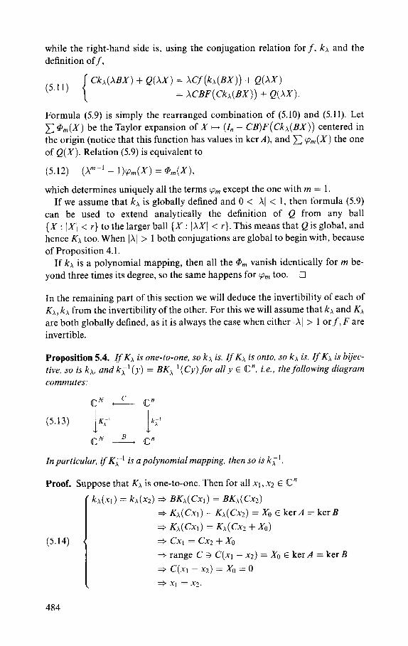
Proposition 5.4. If Kx is one-to-one, so kx is. If KA is onto, so kx is. If Kx is bijec- tive, so is kx, and k;’ (y) = BK<’ (Cy) for ally E C”, i.e., the following diagram commutes:

In particular, if K;’ is a polynomial mapping, then so is k,’

Proof. Suppose that KA is one-to-one. Then for all xi, x2 E C”

’ kx(xl) = kx(xz) + BKx(Cx,) = BKx(Cxz)

+ KA(Cxl) - K,J(CXZ) = A’0 E kerA = kerB

=+ Kx(Cxl) = Kx(Cx2 + Xo)

(5.14) < =+ cx, = cxz + x0

+ range C 3 C(xi -x2) =X0 E kerA = kerB

* C(Xl - x2) = x0 = 0

484

Suppose that KA is onto. Let y E C” be arbitrary. There exists Y E CN such that KA( Y) = Cy. Then

(5.15)

range kx 3 kx(BY) = BKx(CBY) = BKx(CBY +,Y -+CB<)

EkerA

= BKx( Y) = BCy = y.

The inversion formula comes by writing Y = KY’ (Cy) in (5.15). 0

Proposition 5.5. If kx is one-to-one, so is KJ,. If kx is onto, so is KA. If kx is bijec- tive. so is K,J, and

(5.16) K;‘(Y) = Y - Kx(Ck;‘(BY)) + Ck,‘(BY) for all Y E cN.

In particular, ifk,’ is a polynomial mapping, so is KY’, and the degree of Kc’ is not larger than the product of the degrees of Kx and k,‘.

Proof. Suppose that kx is one-to-one and let Xi, Xl E CN. Then

( KA(~I) = &(X2)

(5 7)

l kerB-=kerA E ker B= ker A

=+ Kx(CBxl) + X1 - CBXl = Kx(CB&) +X2 - CBX2 (*)

* BKx(CBX,) = BKx(CBX2)

* kx(BXl) = kX(B&)

=+ BXl = BX2 (using * above)

*x,=x2.

Suppose that kx is onto. Let Y E CN. There exists x E C” such that BY = kx(x) = BKA(Cx). In particular Y - Kx(Cx) E kerA = ker B. Then

(5.18) range KA 3 Kx(Cx+,Y - KJ(Cx!) = Kx(Cx) + Y - Kx(Cx) = Y.

ckerB=kerA

In particular, if kx is bijective just write x = k,‘(BY) to get the inversion for- mula. Finally, if k;’ is a polynomial map, then also kx must be polynomial by a well-known result (see e.g. [16]), and then KA too by Proposition 5.3. q

If we weakened Proposition 5.5 by saying ‘if k,’ and kx arepolynomial mapping, so is K,-‘: then we would not need to resort to the advanced complex analysis result of [16], and the result would extend to the real case too.

6. EXAMPLES

Example 6.1. Consider the 15 x 15 matrix

485

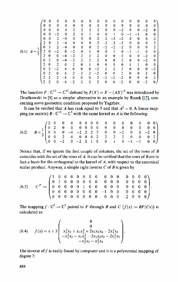
(6.1) ,4=;

( 000000000000000

I 000000000000000 0 0 0 -4 -2 2 2 2 0 0 -2 0 0 -2 0 0 0 -2 o-2 0 10 0 1 0 -1 -1 0 0 0 0 2 -4 0 0 0 2 -2 -2 -2 0 0 0 2 2 0 2 -4 0 0 0 2 -2 -2 -2 0 0 0 2 0 2 2 -4 0 0 0 2 -2 -2 -2 0 0 0 2 2 0 -2 o-2 0 10 0 1 0 -1 -1 0 0 2 0 0 -4 -2 2 2 2 0 0 -2 0 0 -2 0 0 2 0 -4 -2 2 2 2 0 0 -2 0 0 -2 0 20 2 0 2 o-1 0 o-1 0 11 0 0 02-2 4 0 0 o-2 2 2 2 0 0 0 -2 02 0 4 2 -2 -2 -2 0 0 2 0 0 2 0 2 2 2 -4 0 0 0 2 -2 -2 -2 0 0 0 2 2 2 0 -4 -2 2 2 2 0 0 -2 0 0 -2 0 I

The function F : ‘IIll5 -+ @I5 defined by F(X) = X - (AX)*3 was introduced by Druikowski in [9] as a simpler alternative to an example by Rusek [17], con- cerning some geometric condition proposed by Yagzhev.

It can be verified that A has rank equal to 5 and that A2 = 0. A linear map- ping (or matrix) B : 42” + C5 with the same kernel as A is the following:

! 20 0 0 0000 0 0 0 0 0 00

B=; 02 0 0 0000 0 0 0 0 0 00

(6.2) 0 0 0 -4 -2 2 2 2 0 0 -2 0 0 -2 0 0 0 2 -4 0 0 0 2 -2 -2 -2 0 0 0 2 0 0 -2 O-2010 0 1 0 -1 -1 0 0

Notice that, if we ignore the first couple of columns, the set of the rows of B

coincides with the set of the rows of A. It can be verified that the rows of B are in fact a basis for the orthogonal to the kernel of A, with respect to the canonical scalar product. Anyway, a simple right inverse C of B is given by

10000000 0 0 0 0 0 0 0 01000000 0 0 0 0 0 0 0

(6.3) CT:= 0 0 0 0 0 1 0 0 0 0 0 0 0 0 0 . 0 0 0 0 0 0 0 0 -1 0 0 0 0 0 0 00000000 0 0 0 -2 0 0 0

The mapping f : C5 + C5 paired to F through B and C (f(x) := BF(Cx)) is calculated as

(6.4) f(x) = x + 3

0 0

x:x* + ~1x22 + 2x1x2x4 - 2x:x5 -x:x2 -x1x; - 2x1x2x3 -2x:x5

-x;xs - x;xq

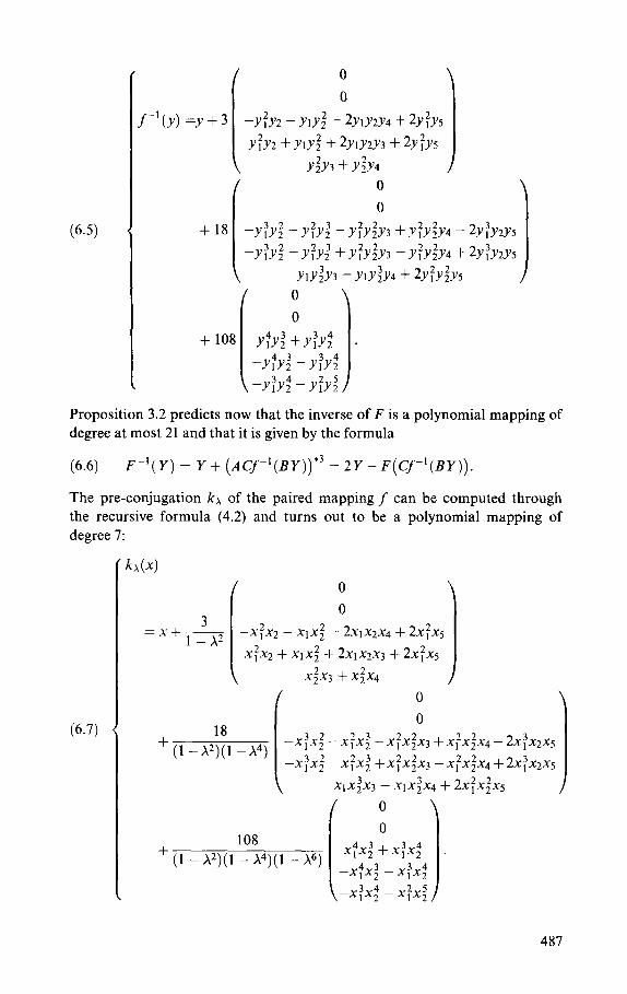
The inverse off is easily found by computer and it is a polynomial mapping of degree 7:

486

(6.5)

P(Y) =Y + 3

I 0

0 + 18 -v:y; -Y:Y: -Y:Y;Ys +Y:Y;YA -2Y:Y2Ys

-Y:Y,2-Y:Y;+Y:Y;Y3 -Y:Y;Y4+2Y:Y2Y5

YlYZY3 - YlY:Y4 + 2Y:Y:Ys

0

0 + 108 YfY;+Y:Y;

; I . -YfYi - v:r;

-YfY24 -Y:Y:

Proposition 3.2 predicts now that the inverse of F is a polynomial mapping of degree at most 21 and that it is given by the formula

(6.6) F-‘(Y) = Y + (ACf.-‘(BY))*3 = 2Y - F(Cf-‘(BY)).

The pre-conjugation kx of the paired mapping f can be computed through the recursive formula (4.2) and turns out to be a polynomial mapping of degree 7:

(6.7)

3 =x+l_X2 ; --x:x2 - x1x2’ - 0 0 2x1x2x4 + 2x:x5

x:x2 + ~1x22 + 2x1x2x3 + 2x:x5

x+3 + xix4

+ (1 -$l -X4)

108

I 0

0

-x:x; - xfxi -x:x:x3 + x;x;x4 - 2x:x2x5

-x:x; - x:x; +x:x,2x3 - x;x;x4 +2x:x2x5

x,x:x, - x,x:x4 + 2x;x;xs

0

0

L I

x;‘x; +x:x; .

-x:x; -x:x;

-x:x; - x:x;

+ (1 - X2)(1 - X4)(1 -X6)

487

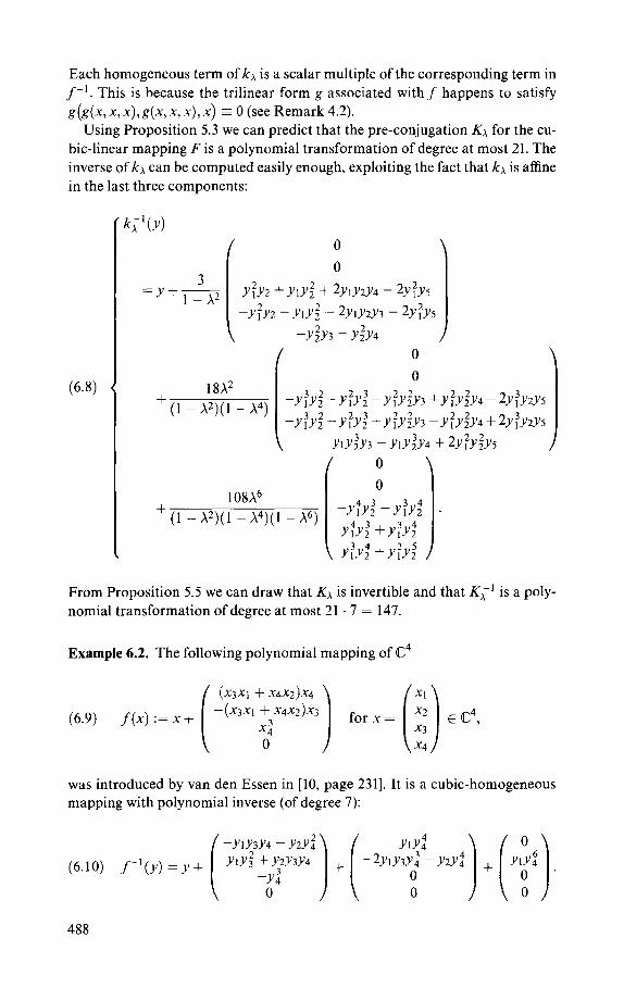
Each homogeneous term of kx is a scalar multiple of the corresponding term in f-l. This is because the trilinear form g associated with f happens to satisfy g(g(x, x, x),g(x, x, x), x) s 0 (see Remark 4.2).

Using Proposition 5.3 we can predict that the pre-conjugation KA for the cu- bic-linear mapping F is a polynomial transformation of degree at most 21. The inverse of k~, can be computed easily enough, exploiting the fact that kx is affine in the last three components:

(6.8)

=y+ 3

1 Y:Y2 YIY; 2YlY2Y4 2Y;Ys

+ + -

- x2

-Y:Y2 - YlYf - 2YylYzY3 - 2Yy:Ys

-Y,2Y3 - Y,2Y4 1

1 8X2

108X6

0

0

-Y:Y; -Y:Y: -Y:Y;Y3 +Y:Y;Y4 -2Y;YzYs

-Y:Y; -Y:Y: +Y:Y;Y3 -Y:Y;Y4+2y;yzys

YlY:Y3 - YlYZY4 + 2y:y;y5

+ (1 -X2)(1 -X4)(1 -X6)

From Proposition 5.5 we can draw that KA is invertible and that KY’ is a poly- nomial transformation of degree at most 21 .7 = 147.

Example 6.2. The following polynomial mapping of C4

(6.9) f(x) := x +

was introduced by van den Essen in [lo, page 2311. It is a cubic-homogeneous mapping with polynomial inverse (of degree 7):

488

YlY,4

-2YlY3Y; - Y2Y44

0 0

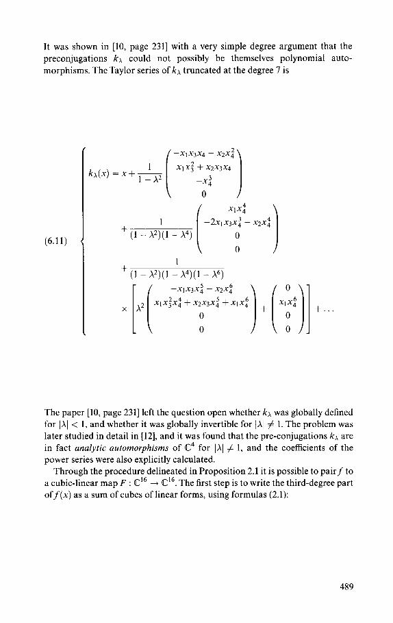
It was shown in [lo, page 2311 with a very simple degree argument that the preconjugations k~ could not possibly be themselves polynomial auto- morphisms. The Taylor series of kx truncated at the degree 7 is

(6.11)

1 kx(x) = x+p

1 - x2

1

-x1x3x4 - x2x;

x,x: + x2x3x4

-.xj

0 I

+ (1 - X2)(1 L)(l -X6)

;( -x,x3x; - x2x46

x x2 x,x:x; + .x:2x3x45 + x1 x46

0

0 11 +...

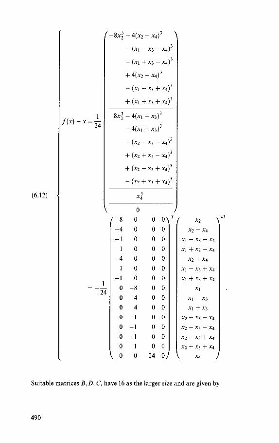
The paper [lo, page 2311 left the question open whether kx was globally defined for ]A] < 1, and whether it was globally invertible for 1x1 # 1. The problem was later studied in detail in [12], and it was found that the pre-conjugations kx are in fact analytic automorphisms of C4 for IA) # 1, and the coefficients of the power series were also explicitly calculated.

Through the procedure delineated in Proposition 2.1 it is possible to pairf to a cubic-linear map F : @I6 -+ C16. The first step is to write the third-degree part off(x) as a sum of cubes of linear forms, using formulas (2.1):

489

(6.12)

f(x) - x = &

1

24

-8x; +4(x2 - x4)3

+ (Xl - x3 -x4)3

- (x1 +x3 - x4)3

+4(X2 +X4)3

- (Xl -x3 +x4)3

+ (Xl +x3 +x4)3

8x; - 4(x1 - x3)3

-4(x1 +x3)3

- (x2 -x3 -x4)3

+ (x2 +x3 - x4)3

+ (x2 - x3 + x4)3

- (x2 +x3 +x4)3

x:

0

‘8 0 00

-4 0 00

-1 0 00

10 00

-4 0 00

10 00

-1 0 00

O-8 00

0 4 00

0 4 00

0 1 00

o-1 00

o-1 00

0 1 00

0 0 -24 0

x2

x2 - x4

x1 -x3 -x4

Xl +x3 -x4

x2 + x4

Xl - x3 + x4

Xl + x3 + x4

Xl

Xl -x3

Xl +x3

x2 - x3 - x4

x2 + x3 - x4

x2 - x3 + x4

x2 + x3 + x4

x4

3

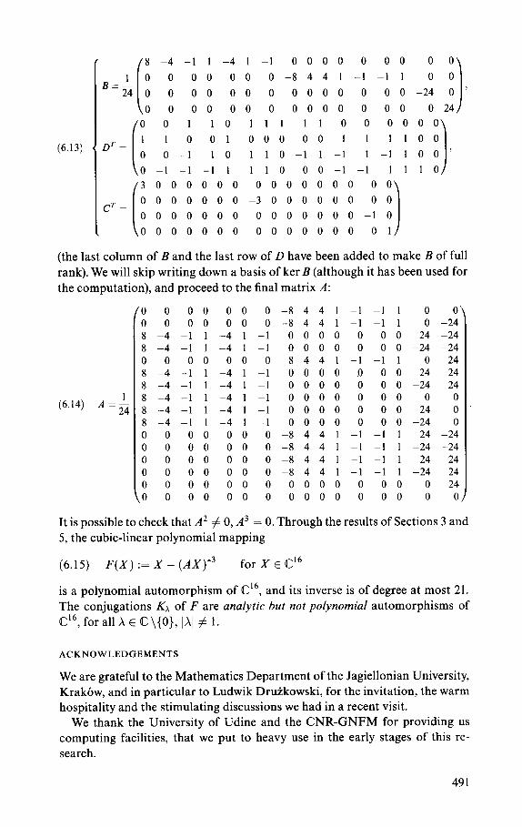
Suitable matrices B, D, C, have 16 as the larger size and are given by

490

(6.13)

t

8

B2 0

24 0

PO

-4 -1 1 -4 1 -1 0000 0 00 0 0

0 00 00 0 -8 4 4 1 -1 -1 1 0 0

0 00 00 0 0000 0 0 0 -24 0

0 00 00 0 0000 0 00 0 24

0 110 111 11 0 0 0 0 0 0

100

1 0 0 ’

D= 110 01 000 00 1 1 1 zz I 0 0 -1 1 0 -1 1 0 -1 1 -1 1 -1

0 -1 -1 -1 1 1 1 0 0 0 -1 -1 1

3000000 0000000 00

CT 0000000-3000000 00 =

0000000 0 0 0 0 0 0 0 -1 0

0000000 0000000 01

(the last column of B and the last row of D have been added to make B of full rank). We will skip writing down a basis of ker B (although it has been used for the computation), and proceed to the final matrix A:

0 0 00 00 0 -8 4 4 1 -1 -1 1 0 o\ 0 0 00 00 0 -8 4 4 1 -1 -1 1 0 -24 8 -4 -1 1 -4 1 -1 0000 0 00 24 -24 8 -4 -1 1 -4 1 -1 0000 0 0 0 -24 -24 0 0 00 00 0 -8 4 4 1 -1 -1 1 0 24 8 -4 -1 1 -4 1 -1 0 0 0 0 0 0 0 24 24 8 -4 -1 1 -4 1 -1 0000 0 0 0 -24 24

(6.14) A =& 8 -4 -1 1 -4 1 -1 0000 0 00 0 0 8 _4 -1 1 -4 1 -1 0000 0 00 24 0’ 8 -4 -1 1 -4 1 -1 0000 0 0 0 -24 0 0 0 00 00 0 -8 4 4 1 -1 -1 1 24 -24 0 0 00 00 0 -8 4 4 1 -1 -1 1 -24 -24 0 0 00 00 0 -8 4 4 1 -1 -1 1 24 24 0 0 00 00 0 -8 4 4 1 -1 -1 1 -24 24 0 0 00 00 0 0000 0 00 0 24

\o 0 00 00 0 0000 0 00 0 o/

It is possible to check that A2 # 0, A3 = 0. Through the results of Sections 3 and 5, the cubic-linear polynomial mapping

(6.15) F(X) := X - (AX)*3 for X E Cl6

is a polynomial automorphism of @16, and its inverse is of degree at most 21. The conjugations Kx of F are analytic but not polynomial automorphisms of @16, for all X E C\(O), 1x1 # 1.

ACKNOWLEDGEMENTS

We are grateful to the Mathematics Department of the Jagiellonian University, Krakow, and in particular to Ludwik Druikowski, for the invitation, the warm hospitality and the stimulating discussions we had in a recent visit.

We thank the University of Udine and the CNR-GNFM for providing us computing facilities, that we put to heavy use in the early stages of this re- search.

491

REFERENCES

I. Arnol’d, V.I. - Geometrical methods in the theory of ordinary differential equations. Springer-

Verlag (1983).

2. Bass. H., E. Connell and D. Wright - The Jacobian conjecture: reduction of degree and formal

expansion of the inverse. Bull. Amer. Math. Sot. 7,2877330 (1982).

3. Bialynicki-Birula, A. and M. Rosenlicht - Injective morphisms of real algebraic varieties. Proc.

Amer. Math. Sot. 13,200-203 (1962).

4. Cima. A., A. van den Essen. A. Gasull, E. Hubbers and F. Mariosas - A polynomial counter-

example to the Markus-Yamabe conjecture. Nijmegen Univ., Dept. of Math., Report No.

9551 (1995). To appear in Adv. Math.

5. Deng, B., G.H. Meisters and G. Zampieri - Conjugation for polynomial mappings. Z. angew.

Math. Phys. ZAMP 46.872-882 (1995).

6. Deng. B. - Analytic conjugation, global attractor. and the Jacobian conjecture. University of

NebraskaaLincoln (1995).

7. Druikowski, L.M. - An effective approach to Keller’s Jacobian conjecture. Math. Ann. 264,

303-313 (1983).

8. Druikowski, L.M. and K. Rusek -The formal inverse and the Jacobian conjecture. Ann. Polon.

Math. 46.85-90 (1985).

9. Druikowski, L.M. - The Jacobian conjecture. Institute of Mathematics, Polish Academy of

Sciences, Preprint 492 (1991).

10. Essen. A. van den (Editor) ~ Automorphisms of Affirm Spaces. Proceedings of the CuraGao

Conference, July 4-8,1994, Kluwer Academic Publishers (1995).

11. Essen, A. van den and E. Hubbers - Chaotic polynomial automorphisms; counterexamples to

several conjectures. Adv. in Appl. Math. 18, 382-388 (1997).

12. Gorni, G. and G. Zampieri - On the existence of global analytic conjugations for polynomial

mappings of Yagzhev type. J. Math. Anal. Appl. 201,880&896 (1996).

13. Gorni, G. and G. Zampieri - Yagzhev polynomial mappings: on the structure of theTaylor ex-

pansion of their local inverse. Ann. Polon. Math. 64.2855290 (1996).

14. Keller. O.H. - Ganze Cremona transformationen. Monatshefte fur Mathematik und Physik 47,

299- 306 (1939).

15. Rabier. P.J. On components of polynomial automorphisms in two variables. Comm. in Alge-

bra 24.929-937 (1996).

16. Rudin, W. - lnjective polynomial maps are automorphisms. Amer. Math. Monthly 102,

540-543 (1995).

17. Rusek, K. - A geometric approach to Keller’s Jacobian conjecture. Math. Ann. 264, 315-320

(1983).

18. Yagzhev, A.V. - Keller’s problem. Siberian Math. J. 21, 7477754 (1980).

Received September 1996

492