Embed Size (px)
Citation preview

arX
iv:1
204.
2227
v2 [
quan
t-ph
] 1
1 D
ec 2
012
An algebraic approach to the study of multipartite
entanglement
S. Di Martino
Dipartimento di Matematica dell’Universita di Bari, Via Orabona 4, 70125 Bari, Italy
B. Militello
Dipartimento di Fisica dell’Universita di Palermo, Via Archirafi 36, 90123 Palermo,
Italy
A. Messina
Dipartimento di Fisica dell’Universita di Palermo, Via Archirafi 36, 90123 Palermo,
Italy
Abstract. A simple algebraic approach to the study of multipartite entanglement
for pure states is introduced together with a class of suitable functionals able to
detect entanglement. On this basis, some known results are reproduced. Indeed,
by investigating the properties of the introduced functionals, it is shown that a subset
of such class is strictly connected to the purity. Moreover, a direct and basic solution
to the problem of the simultaneous maximization of three appropriate functionals for
three-qubit states is provided, confirming that the simultaneous maximization of the
entanglement for all possible bipartitions is compatible only with the structure of
GHZ-states.

An algebraic approach to the study of multipartite entanglement 2
1. Introduction
Entanglement plays an important role in applications of quantum mechanics to
nanotechnologies, especially in the field of quantum information and communication.
The concept of entanglement is mathematical, since it corresponds, in the case of pure
states, to the impossibility of writing the quantum state describing a compound physical
system as a simple product of states related to the single subsystems. Nevertheless, this
mathematical property of the state has interesting physical implications, such as the
presence of non classical correlations between quantum systems, even when they are
quite far from each other (non locality).
In spite of the strong interest and deep studies developed on this subject, detection
and classification of entanglement in multipartite systems are unsolved problems up
to date. Indeed, it has not yet been defined a universal quantity able to measure the
entanglement level to be associated to a generic pure or even mixed state. (The concept
of non entangled state is translated into factorizability for pure states and separability
— simple or generalized — for mixed states, though the latter concept includes the
former as a special case.) Besides, there are properties that any measurement of
entanglement should possess. In particular, it must be discriminant (vanishing iff
the state is separable), not increasing under LOCC (local operations and classical
communication) and convex (it must not increase when two or more states are combined
in a mixture) [1].
Though a general answer to measurement and detection of entanglement is absent,
if the system is composed by a few of low dimensional subsystems it is possible to
provide conditions for the presence of entanglement, but rarely these conditions are
both necessary and sufficient. In 1996, Peres [2] introduced a sufficient condition for
the detection of bipartite entanglement that can be written in terms of a functional
addressed as negativity, subsequently studied by Horodecki et al, who have proven that
this condition is necessary and sufficient for low-dimensional systems [3, 4]. Another
important functional is the concurrence introduced by Wootters in [5, 6], which is a true
measure of entanglement, both for pure and mixed states, but unfortunately applicable
only to systems which are couples of two level systems (i.e., a couple of qubits).
The study of multipartite entanglement is more complex [7, 8, 9], not only from
the computational point of view, but even at a conceptual level, since for instance it is
neither immediate nor intuitive to understand what is a state with a maximum level of
multipartite entanglement. In 2008, Sabin et al, [10], tried to extend the negativity
to the tripartite case, succeeding in finding a functional that detects the tripartite
entanglement when applied to pure states. However, this functional gives only a clue
about the presence of entanglement in mixed states, indeed in this case the condition
given is neither necessary nor sufficient. Nevertheless, its effectiveness has been shown
in the study of simple physical systems [11]. Another interesting quantity, introduced
for detecting entanglement of pure states of three qubits, is the three-tangle [12], which
is based on the concurrence and whose validity has been criticized [13]. Recently, a

An algebraic approach to the study of multipartite entanglement 3
classification of entangled states for three-qubit states has been given on the basis of
some invariant quantities [14]. Moreover, attempts to apply well known results of algebra
or geometry to study multipartite entanglement have been made. In [15], for instance,
Makela et al associated to every pure state of N-qubits a polynomial, characterizing
completely the state, capable not only to detect factorizability of the state but even the
number of separable qubits. Instead, in [16], Miyake used the hyperdeterminants and
the theory of Segre variety to give a classification of the entanglement of pure states in
tripartite systems. A very useful tool to study multipartite entanglement in mixed states
is given by the necessary condition for separability expressed by Huber et al [17], which
exploits a correlation function defined through replicas of the states under scrutiny and
operators of partial swapping, and which has been exploited to reveal thermal tripartite
correlations in spin-star systems [18].
Another important quantity that has been used to reveal entanglement in several
cases (bipartite and multipartite systems), is the purity (strictly connected to the linear
entropy [19]) of the reduced density matrix, which in passing is strictly connected with
the concept of mixedness [20]: the more two systems are entangled, the less pure is the
reduced state describing each one of the two systems.
In this paper we reproduce some known results about entanglement detection
by introducing a simple algebraic approach to establish whether a pure state of a
multipartite system is entangled with respect to a given bipartition. Through this
analysis it is possible to determine whether a given pure state is completely separable,
separable or totally entangled. In the last case one can infer the presence of genuine
multipartite entanglement. On the basis of this approach, we naturally introduce a class
of functionals which includes, among others, quantities traceable back to the purity and
the linear entropy, strictly related to the so called concurrence vectors, presented in [21]
by Akhtarshenas and studied by Mintert et al in [22, 23].
The paper is organized as follows. In the next section we describe our approach
to the study of multipartite entanglement and give the definition of a relevant class
functionals, proving the ability of such quantities to detect entanglement in pure states.
In section 3 we show that such quantities are strictly connected with purity and
mixedness. In section 4 we show, by exploiting our simple and algebraic approach, that
in the case of three qubits, simultaneous maximization of the three relevant functionals
is possible only for states equivalent (i.e., equal up to a local and unitary transformation)
to the GHZ state. Finally, in the last section, we give some comments and concluding
remarks.
2. Factorizability conditions
Each pure state of a bipartite system can be written in the form:
|φ〉 =∑
i,j
aij |ij〉 , (1)

An algebraic approach to the study of multipartite entanglement 4
where we take {|ij〉} as a standard basis in the Hilbert space H = H1 ⊗H2. This state
is said factorizable if it can be written in the form:
(∑
i
αi |i〉)(∑
j
βj |j〉). (2)
This means that the state is factorizable iff aij = αiβj, ∀i, j. So, introducing the
matrix of the probability amplitudes A = (aij), the state |φ〉 is factorizable iff columns
(respectively rows) span a 1-dimensional subspace, i.e. rankA = 1.
In general, this means detA = 0 and in the case of a two qubits system, in [24] it is
proven that this condition is equivalent to the Peres-Horodecki criterion. The condition
here expressed can be easily extended to investigate the presence of entanglement in
every pure states of multipartite systems. We can summarize this result for bipartite
systems with the following theorem.
Theorem 1. A pure state of a bipartite m× n system is factorizable iff the rank of the
corresponding matrix of the probability amplitudes is unity.
Now we can extend this result to tripartite systems and we can generalize it to
every multipartite system. Consider a m × n × p Hilbert space. Each pure state |φ〉living in it can be written in the form:
|φ〉 =m−1∑
i=0
n−1∑
j=0
p−1∑
k=0
aijk|ijk〉, (3)
where {|ijk〉} is the standard product basis for the Hilbert space related to the whole
system. Again, the state is factorizable with respect, for instance, to the first component,
iff:
aijk = αiβjk ∀i, j, k. (4)
This time the matrix of the probability amplitudes is a cubic one and the
separability condition of the first component can be traced back to the proportionality
of the layers in the direction of i. For a better visualization of this statement we can
write two layers in the i-direction:
αrβ11 · · · αrβ1p· · ·αrβn1 · · · αrβnp
,
αsβ11 · · · αsβ1p· · ·αsβn1 · · · αsβnp
,
which are the rth and sth layers.
Starting from these considerations, we can prove the following theorem.
Theorem 2. A pure state |φ〉 in a m× n× p Hilbert space is factorizable iff one of the
following is true:
• aijkai′j′k′ − aij′k′ai′jk = 0 , ∀i, j, k, i′, j′, k′;• aijkai′j′k′ − ai′jk′aij′k = 0 , ∀i, j, k, i′, j′, k′;

An algebraic approach to the study of multipartite entanglement 5
• aijkai′j′k′ − ai′j′kaijk′ = 0 , ∀i, j, k, i′, j′, k′.
Proof. For the sake of simplicity and without loss of generality, let us consider the
factorizability condition for the first qubit.
If the state |φ〉 is factorizable with respect to such first qubit, using the
factorizability condition in equation (4) we have:
αiβjkαi′βj′k′ − αiβj′k′αi′βjk = 0. (5)
Vice versa, if we suppose aijkai′j′k′ −aij′k′ai′jk = 0, ∀i, j, k, i′, j′, k′ then, fixing i, j, k such
that aijk 6= 0, it turns out that:
ai′j′k′ =ai′jkaijk
aij′k′ = αi′βj′k′ , ∀i′, j′, k′, (6)
where we take αi′ =ai′jkaijk
and βj′k′ = aij′k′, which is the factorizability condition of the
first component.
Using this theorem we can define a class of functionals able to detect entanglement
in each pure state of a tripartite system.
Let f : C → R be a positive function such that ∀x ∈ C f(x) ≥ 0 and f(x) = 0 iff
x = 0, then we have the following:
Theorem 3. A pure state |φ〉 in a m × n × p Hilbert space is factorizable iff at least
one of the following is true:
• M(f)1 :=
∑i,j,k,i′,j′,k′ f(aijkai′j′k′ − aij′k′ai′jk) = 0;
• M(f)2 :=
∑i,j,k,i′,j′,k′ f(aijkai′j′k′ − ai′jk′aij′k) = 0;
• M(f)3 :=
∑i,j,k,i′,j′,k′ f(aijkai′j′k′ − ai′j′kaijk′) = 0.
The proof of this result follows immediately from the theorem 2 and from the
properties of f .
We can make some observation about this. Firstly, if M(f)k = 0 then the
corresponding state is factorizable with respect to the kth component, so if two of these
quantities are zero also the third has to be equal to zero (considering that, for pure
states, if two of the three subsystems are separable, then the third one is separable as
well). This statement can be easily proven considering the factorizability condition in
equation (4) for two of the three components. Secondly, if all the three M(f)k are equal
to zero than the state is completely factorizable — i.e., it is the product of three states
of the three subsystems — and if each one of them is different from zero the state is
genuinely tripartite entangled.
Theorem 3 can be extended to the multipartite case considering all the possible
bipartitions of the system. For instance, in the case of a quadripartite system we have
seven conditions given by:
• M(f)1 :=
∑i,j,k,l,i′,j′,k′,l′ f(aijklai′j′k′l′ − aij′k′l′ai′jkl) = 0;

An algebraic approach to the study of multipartite entanglement 6
• M(f)2 :=
∑i,j,k,l,i′,j′,k′,l′ f(aijklai′j′k′l′ − ai′jk′l′aij′kl) = 0;
• M(f)3 :=
∑i,j,k,l,i′,j′,k′,l′ f(aijklai′j′k′l′ − ai′j′kl′aijk′l) = 0;
• M(f)4 :=
∑i,j,k,l,i′,j′,k′,l′ f(aijklai′j′k′l′ − ai′j′k′laijkl′) = 0;
• M(f)12 :=
∑i,j,k,l,i′,j′,k′,l′ f(aijklai′j′k′l′ − aijk′l′ai′j′kl) = 0;
• M(f)13 :=
∑i,j,k,l,i′,j′,k′,l′ f(aijklai′j′k′l′ − aij′kl′ai′jk′l) = 0;
• M(f)23 :=
∑i,j,k,l,i′,j′,k′,l′ f(aijklai′j′k′l′ − ai′jkl′aij′k′l) = 0.
where M(f)k functionals are related to separation of the k-th subsystem when the other
three are considered as a whole, while M(f)kj ’s are related to the bipartition obtained by
considering the couple k−j as a whole and the other two parts as the second subsystem
of the bipartition.
3. Connection with the Purity
In this section we prove that if we take as function f the squared modulus, the relevant
functionals, simply denoted as Mk, are strictly connected with the purity of the relevant
reduced density operators. To this end, let us first of all rewrite Mk by considering
only two indexes (this means that the two indexes, say i and j, will span multipartite
subsystems):
Mk =∑
i,j,i′,j′
|aijai′j′ − aij′ai′j |2. (7)
Then, by expanding the modulus, one gets:
Mk =∑
i,j,i′,j′
(aija∗ijai′j′a
∗i′j′ + aij′a
∗ij′ai′ja
∗i′j − aijai′j′a
∗ij′a
∗i′j − a∗ija
∗i′j′aij′ai′j)
= 2(1 − p) (8)
where
p =∑
i,j,i′,j′
aijai′j′a∗ij′a
∗i′j =
∑
i,j,i′,j′
a∗ija∗i′j′aij′ai′j , (9)
is the purity of the density operator associated to any of the two subsystems constituting
the bipartition. This makes the functional Mk essentially equal (up to the factor 2) to
the linear entropy (mixedness) [20].
Therefore, the quantities Mk are invariant under local unitary transformations and
are bounded as follows: 0 ≤Mk ≤ 2(D−1)/D, where D is the dimension of the smaller
among the two Hilbert subspaces associated to the bipartition considered. Moreover,
maximization is reached when the whole-system state can be written as a superposition
of D states with the same weights:
|ψ〉 = D−1/2D∑
j=1
eiχj |j〉k |Φj〉k , (10)

An algebraic approach to the study of multipartite entanglement 7
Figure 1. Matrix of the probability amplitudes related to the W-state. The vertexes
of the first layer correspond (from top-part left-side, clockwise) to the coefficients: a000,
a001, a011, a010; the vertexes of the second layer instead correspond to the coefficients:
a100, a101, a111, a110.
where |j〉k and |Φj〉k refer to the two subsystems constituting the bipartition, and
〈j| l〉 = 〈Φj | Φl〉 = δjl.
3.1. Some Examples
For a better understanding of the results given in the previous section we apply the
previously proven criteria to some pure states. First of all, let us consider the W-state
which, as well known, is genuinely tripartite entangled:
|W 〉 =1√3
(|100〉 + |010〉 + |001〉). (11)
The relevant cubic matrix of probability amplitudes is shown in fig.1.
A rapid calculation gives:
M1 = M2 = M3 =8
9, (12)
and therefore, the state is genuinely tripartite entangled in accordance with theorem 3.
As a second example, let us consider the GHZ-state:
|GHZ〉 =1√2
(|000〉 + |111〉), (13)
whose matrix of the probability amplitudes is shown in fig. 2.

An algebraic approach to the study of multipartite entanglement 8
Figure 2. Matrix of the probability amplitudes related to the GHZ-state. The vertex-
coefficient correspondence is the same as in the previous figure.
Once again a straightforward calculation leads to:
M1 = M2 = M3 = 1. (14)
By the way, we mention that in the following section we prove unity to be the
maximum value that these quantities can reach for a three-qubit system. Moreover, it
is worth noting that maximization of two Mk does not imply maximization of the third,
as shown by the following example. Indeed, consider the state:
|ψbis〉 =1√2|000〉 +
1√2|011〉 , (15)
which is factorizable with respect to the first qubit, being M1 = 0, but it is not
factorizable with respect to the other two qubits, being M2 = M3 = 1.
Finally, let us consider a state for which it is not evident whether it is entangled or
not:
|ϕ〉 =1
2√
26(5 |000〉 + 3 |010〉 + 2 |001〉 + 4 |011〉 + 7 |101〉 + |111〉), (16)
Since it turns out that M1 ≈ 0.88, M2 ≈ 0.42 and M3 ≈ 0.70 we can conclude that it is
a genuinely tripartite entangled state.
4. Maximization of M-quantities for a three qubit system
In the second example of section 2 we proved that for the GHZ-state all the Mk’s reach
their maximum value. In this section we prove that all pure states of three qubits for
which Mk = 1 ∀k are equivalent to the GHZ-state, i.e. there exists a local and unitary
transformation that maps this state into GHZ-state.
Our simple and basic approach makes more transparent the proof of this statement
in comparison with the proof given in [25].

An algebraic approach to the study of multipartite entanglement 9
Consider a three qubits pure state |ψ〉 for which it is valid the hypothesis Mk = 1 ∀k.
Since for this state the Mk reach their maximum, we can write the state in the following
form:
|ψ〉 =1√2|0〉k |φ0〉k +
1√2eiχ |1〉k |φ1〉k , (17)
where k refers to the two indexes different from k, {|0〉 , |1〉} is the standard basis of the
kth qubit and |φ0〉 and |φ1〉 are such that 〈φa| φb〉 = δab for a, b = 0, 1, simply applying
a Schmidt’s decomposition.
By the way, we note that in the case of two qubits, maximization of the unique
M-functional leads to a Bell-like structure.
In the tripartite case, because of the simultaneous maximization of the three Mk’s,
we have that this structure is valid for each of the three qubits.
Moreover, this structure is left unchanged by any unitary and local transformation.
Let us consider this structure with respect to the first qubit and, applying
again a Schmidt’s decomposition, we can convert the state |φ0〉23 in (cos θ1 |00〉23 +
eiχ1 sin θ1 |11〉23), getting:
|ψ〉 =1√2|0〉1 (cos θ1 |00〉23 + eiχ1 sin θ1 |11〉23)
+1√2eiχ |1〉1 [|0〉2 (a |0〉3 + b |1〉3) + |1〉2 (c |0〉3 + d |1〉3)], (18)
where {|0〉l , |1〉l} is a basis, not necessarily standard, for the lth qubit, and a, b, c, d
are complex numbers and every coefficient satisfies the normalization and orthogonality
condition between the two states |φ0〉23 and |φ1〉23.Now we can decompose the state |ψ〉 with respect to the second qubit, getting:
|ψ〉 =1√2|0〉2 [cos θ1 |00〉13 + eiχ |1〉1 (a |0〉3 + b |1〉3)]
+1√2|1〉2 [eiχ1 sin θ1 |01〉13 + eiχ |1〉1 (c |0〉3 + d |1〉3)]. (19)
The orthogonality conditions involves the orthogonality between the two states
(a |0〉3 + b |1〉3) and (c |0〉3 + d |1〉3), which implies a = α cos θ2, b = αeiχ2 sin θ2,
c = βe−iχ2 sin θ2 and d = β cos θ2.
In addition, exploiting the normalization constrain with respect to the first qubit,
we find α = cos θ3 and β = eiχ3 sin θ3, so that we can rewrite the state in equation (18)
as:
|ψ〉 =1√2|0〉1 |φ0〉23 +
1√2eiχ |1〉1 |φ1〉23 , (20)
where

An algebraic approach to the study of multipartite entanglement 10
|φ0〉23 = (cos θ1 |00〉23 + eiχ1 sin θ1 |11〉23)
and
|φ1〉23 = cos θ3 |0〉2 (cos θ2 |0〉3 + eiχ2 sin θ2 |1〉3+ eiχ3 sin θ3 |1〉2 (e−iχ2 sin θ2 |0〉3 − cos θ2 |1〉3).
Summarizing, we impose the normalization condition of |φ0〉 e |φ1〉 with respect to
the first qubit and the orthogonality condition with respect to the second qubit. We now
have to enforce: 1)The orthogonality condition with respect to the first qubit; 2)The
normalization condition with respect to the second qubit; 3)The orthogonality condition
with respect to the third qubit; 4)The normalization condition with respect to the third
qubit.
The orthogonality condition for the first qubit leads to eiχ cos θ1 cos θ2 cos θ3 −ei(χ+χ3−χ1) sin θ1 cos θ2 sin θ3 = 0, and so we have the condition:
θ2 =π
2∨ cos θ1 cos θ3 − ei(χ3−χ1) sin θ1 sin θ3 = 0. (21)
Rewriting the state |ψ〉 as,
|ψ〉 =1√2|0〉2 [cos θ1 |00〉13 + eiχ cos θ3 |1〉1 (cos θ2 |0〉3 + eiχ2 sin θ2 |1〉3)]
+1√2|1〉2 [sin θ1 |01〉13 (22)
+ ei(χ+χ3) sin θ3 |1〉1 (e−iχ2 sin θ2 |0〉3 − cos θ2 |1〉3)],
the normalization condition for the second qubit leads to (cos2 θ1 + cos2 θ3 cos2 θ2 +
cos2 θ3 sin2 θ2 = 1), that is,
cos θ3 = sin θ1, (23)
and likewise for the other state (we consider only this case because possible sign
difference between sine and cosine can be described by adjusting the phase factors).
Now, we decompose the state with respect to the third qubit:
|ψ〉 =1√2|0〉3 |φ′
0〉12 +1√2|1〉3 |φ′
1〉12 , (24)
where
|φ′0〉12 = (cos θ1 |00〉12 + eiχ cos θ3 cos θ2 |10〉12
+ ei(χ+χ3−χ2) sin θ3 sin θ2 |11〉12)

An algebraic approach to the study of multipartite entanglement 11
and
|φ′1〉12 = (eiχ1 sin θ1 |01〉12 + ei(χ+χ2) cos θ3 sin θ2 |10〉12
− ei(χ+χ3) sin θ3 cos θ2 |11〉12),and we impose the third condition (orthogonality with respect to the third qubit):
(eiχ2 cosθ3 cos θ2 sin θ2 − eiχ2 sin2 θ3 cos θ2 sin θ2 = 0), that leads to
θ3 =π
4∨ θ2 = 0 ∨ θ2 =
π
2, (25)
(again we consider only θ3 = π4
because possible sign difference between sin θ3 and cos θ3can be englobed in the phase factors).
Summarizing, we can have three possible situations:
θ3 = π4⇒ θ1 = π
4;
θ2 = 0;
θ2 = π2.
(26)
The normalization condition at point 4, cos2 θ1 + cos2 θ3 cos2 θ2 + sin2 θ3 sin2 θ2 = 1
is automatically satisfied for θ3 = π4
and θ1 = π4
as for θ2 = 0. Instead, if θ2 = π2
then
necessarily θ1 = θ3 = π4.
We can apply the conditions we have found, writing the initial state as:
1√2|0〉1 (sin θ3 |00〉23 + eiχ1 cos θ3 |11〉23)
+1√2eiχ |1〉1 [cos θ3 |0〉2 (cos θ2 |0〉3 + eiχ2 sin θ2 |1〉3) (27)
+ eiχ3 sin θ3(e−iχ2 sin θ2 |0〉3 − cos θ2 |1〉3)],
where parameters vary in the following way:
θ3 = π4
∀θ2;
θ2 = 0 ∀θ3;(28)
It remains to prove that this state is equivalent to the GHZ under local unitary
transformation.
If θ2 = 0, condition (21) assures either χ1 = χ3 or θ3 = 0 or θ3 = π2. Let us examine
these three possibilities.
If θ2 = 0 and θ3 = 0 the state becomes:
1√2eiχ3 |011〉 +
1√2eiχ |100〉 , (29)
and we can easily find a transformation that sends it in the GHZ.

An algebraic approach to the study of multipartite entanglement 12
If θ2 = 0 and θ3 = π2
then we have the state:
1√2|000〉 − 1√
2ei(χ+χ3) |111〉 , (30)
and even in this case we can easily find the transformation needed.
If, finally, θ2 = 0 and χ1 = χ3 the state becomes:
1√2|0〉1 (sin θ3 |00〉23 + eiχ3 cos θ3 |11〉23)
+1√2eiχ |1〉1 (cos θ3 |00〉23 − eiχ3 sin θ3 |11〉23),
(31)
and it is converted in the GHZ by:
sin θ3 |0〉1 + eiχ cos θ3 |1〉1 →∣∣∣0⟩
eiχ3 cos θ3 |0〉1 − ei(χ+χ3) sin θ3 |1〉1 →∣∣∣1⟩ (32)
We have now to examine the first case of eq.(28), which is θ3 = π4. In this analysis
we have to distinguish the two cases θ2 = π2
and θ2 6= π2.
If θ3 = π4
and θ2 6= π2, the state has the form:
1√2|0〉1
(1√2|00〉23 +
1√2eiχ3 |11〉23
)
+1√2|1〉1 [
1√2|0〉2 (cos θ2 |0〉3 + eiχ2 sin θ2 |1〉3) (33)
+1√2eiχ3 |1〉2 (e−iχ2 sin θ2 |0〉3 − cos θ2 |1〉3)],
(remember the (21) assures χ1 = χ3).
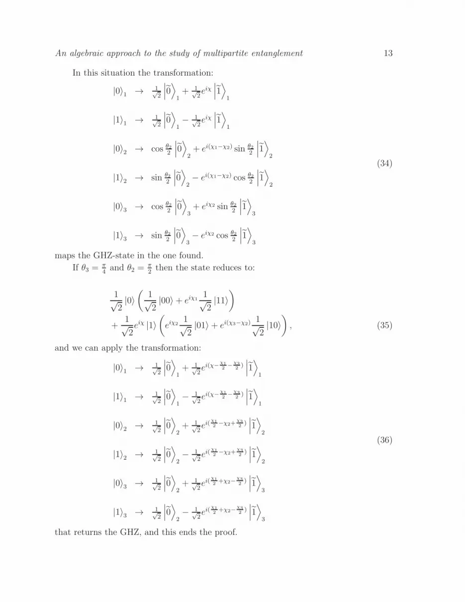
An algebraic approach to the study of multipartite entanglement 13
In this situation the transformation:
|0〉1 → 1√2
∣∣∣0⟩
1+ 1√
2eiχ
∣∣∣1⟩
1
|1〉1 → 1√2
∣∣∣0⟩1− 1√
2eiχ
∣∣∣1⟩1
|0〉2 → cos θ22
∣∣∣0⟩
2+ ei(χ1−χ2) sin θ2
2
∣∣∣1⟩
2
|1〉2 → sin θ22
∣∣∣0⟩
2− ei(χ1−χ2) cos θ2
2
∣∣∣1⟩
2
|0〉3 → cos θ22
∣∣∣0⟩3
+ eiχ2 sin θ22
∣∣∣1⟩3
|1〉3 → sin θ22
∣∣∣0⟩
3− eiχ2 cos θ2
2
∣∣∣1⟩
3
(34)
maps the GHZ-state in the one found.
If θ3 = π4
and θ2 = π2
then the state reduces to:
1√2|0〉
(1√2|00〉 + eiχ1
1√2|11〉
)
+1√2eiχ |1〉
(eiχ2
1√2|01〉 + ei(χ3−χ2)
1√2|10〉
), (35)
and we can apply the transformation:
|0〉1 → 1√2
∣∣∣0⟩
1+ 1√
2ei(χ−
χ1
2−χ3
2)∣∣∣1⟩
1
|1〉1 → 1√2
∣∣∣0⟩1− 1√
2ei(χ−
χ1
2−χ3
2)∣∣∣1⟩1
|0〉2 → 1√2
∣∣∣0⟩
2+ 1√
2ei(
χ1
2−χ2+
χ3
2)∣∣∣1⟩
2
|1〉2 → 1√2
∣∣∣0⟩
2− 1√
2ei(
χ1
2−χ2+
χ3
2)∣∣∣1⟩
2
|0〉3 → 1√2
∣∣∣0⟩2
+ 1√2ei(
χ1
2+χ2−
χ3
2)∣∣∣1⟩3
|1〉3 → 1√2
∣∣∣0⟩
2− 1√
2ei(
χ1
2+χ2−
χ3
2)∣∣∣1⟩
3
(36)
that returns the GHZ, and this ends the proof.

An algebraic approach to the study of multipartite entanglement 14
5. Discussion
In this paper, by introducing a simple algebraic approach we have reproduced some
known results which provide recipes to establish whether a certain multipartite pure
state is entangled with respect to a given bipartition. Such an analysis allows to
determine whether the pure state describing a system is completely separable, separable
or totally entangled. In the last case one can say that such a state possesses genuine
multipartite entanglement.
Our treatment naturally led us to introduce a class of functionals which include
quantities traceable back to the concepts of purity and linear entropy. Moreover,
we have dealt with the problem of the simultaneous maximization of the relevant
functionals (purities of the reduced matrices), providing an alternative proof to the
known result that in the case of three qubits the only states that maximize all the
relevant functionals are the GHZ-state and all the equivalent states (i.e., equal up to
local unitary transformations).
This preliminary studies paves the way to the analysis of multipartite entanglement
in cases wherein more than three subsystems are involved. In particular, simultaneous
maximization of the relevant functionals for N -partite systems — with N ≥ 4 — could
provide interesting results and ideas in the study of maximal multipartite entanglement.
It is of relevance to stress in addition that other known functionals might be found in
the class we have introduced, or, alternatively, new quantities could be introduced and
their properties explored.
6. Acknowledgements
The authors wish to thank D. Chruscinski, H. de Guise, A. Jamio lkowski and M.
Michalski for stimulating discussions. The authors express their gratitude to P. Facchi
for interesting suggestions and for carefully reading the manuscript.
[1] V. Vedral and M. B. Plenio, Phys. Rev. A 57, 1619 (1997).
[2] A. Peres, Phys. Rev. Lett. 77, 1413 (1996).
[3] P. Horodecki, Phys. Lett. A 232, 333 (1997).
[4] R. Horodecki, P. Horodecki, M. Horodecki and K. Horodecki, Rev. Mod. Phys. 81, 865 (2009).
[5] S. Hill and W. K. Wotters, Phys. Rev. Lett. 78, 5022 (1997).
[6] W. K. Wootters, Phys. Rev. Lett. 80, 2245 (1998).
[7] L. Amico, R. Fazio, A. Osterloh and V. Vedral, Rev. Mod. Phys. 80, 517 (2008).
[8] V. I. Man’ko, G. Marmo, E. C. G. Sudarshan and F. Zaccaria, J. Phys. A: Math. Gen. 35, 7137
(2002) .
[9] P. Facchi, Rend. Lincei Mat. Appl. 20, 25-67 (2009).
[10] C. Sabin and G. Garcia-Alcaine, Eur. Phys. J. D. 48, 435-442 (2008).
[11] F. Anza, B. Militello and A. Messina, J. Phys. B 43, 205501 (2010).
[12] V. Coffman, J. Kundu and W. K. Wootters, Phys. Rev. A 61, 052306 (2000).
[13] E. Jung, D. Park and J. W. Son, Phys. Rev. A 80, 010301 (2009).
[14] H. A. Carteret and A. Sudbery, J. Phys. A: Math. Gen. 33, 4981 (2000).
[15] H. Makela and A. Messina, Phys. Rev. A 81, 012326 (2010).
[16] A. Miyake, Phys. Rev. A 67, 012108 (2003).

An algebraic approach to the study of multipartite entanglement 15
[17] M. Huber, F. Mintert, A. Gabriel and B. C. Hiesmayar, Phys. Rev. Lett. 104, 210501 (2010).
[18] B. Militello and A. Messina, Phys. Rev. A 83, 042305 (2011).
[19] U. Fano, Rev. Mod. Phys. 29, 74 (1957).
[20] G. Jaeger, A. V. Sergienko, B. E. A. Saleh and M. C. Teich, Phys. Rev. A 68, 022318 (2003).
[21] S. J. Akhtarshenas, J. Phys. A: Math. Gen. 38 (2005) 67776784.
[22] F. Mintert, M. Kus and A. Buchleitner Phys. Rev. Lett. 92, 167902 (2004).
[23] F. Mintert, M. Kus and A. Buchleitner Phys. Rev. Lett. 95, 260502 (2005).
[24] S. Shelly Sharma and N. K. Sharma, Phys. Rev. A 82, 012340 (2010).
[25] J. Schlienz and G. Mahler, Phys. Lett. A 224 (1996) 39-44


