Cylindrical Algebraic Sub-Decompositions

D. J. Wilson, R. J. Bradford, J. H. Davenport and M. England

Abstract. Cylindrical Algebraic Decompositions (CADs) have been studied since their creation asa tool for working with semi-algebraic sets and eliminating quantifiers of the reals. In this paper weare concerned with Cylindrical Algebraic Sub-Decompositions (sub-CADs), defined as subsets ofCADs sufficient to describe the solutions for given formulae. We discuss several ways to constructsub-CADs, both from new work and the literature, and we demonstrate their interaction.

We define a manifold sub-CAD as those cells in a CAD lying on a designated manifold anda layered sub-CAD as those cells with prescribed dimensions. We present algorithms to produceboth and then describe how the ideas may be combined with each other, as well as their interactionwith the recent theory of Truth-Table Invariant CAD (TTICAD). We give a complexity analysis formanifold sub-CADs and 1-layered manifold sub-CADs and present examples where these techniquescan be of use, offering substantial savings on previous approaches. All concepts have been fullyimplemented in a Maple package and examples demonstrate that they can offer substantial savings.

Keywords. Cylindrical Algebraic Decomposition, Real Algebraic Geometry, Equational Constraints,Symbolic Computation, Computer Algebra.MSC Code: 68W30 (Symbolic Computation and Algebraic Computation).

1. Introduction

1.1. Motivation

A cylindrical algebraic decomposition (CAD) is a decomposition of Rn into cells arranged cylindrically(so the projections of any pair of cells are either equal or disjoint) each of which is describable usingpolynomial relations. They are produced to answer a problem, originally sign-invariance with respectto a list of polynomials, meaning each polynomial had constant sign on each cell. First introduced byCollins in [14], CAD has become a key tool in real algebraic geometry for studying semi-algebraic setsand eliminating quantifiers. Other applications include robot motion planning [35], parametric opti-misation [24], epidemic modelling [11], theorem proving [33] and programming with complex functions[18].

However, it has often been noted that CAD usually produces far more information that requiredto solve the underlying problem. Often it will produce thousands of superfluous cells which are notrelevant to the solution set. Many techniques have been developed to try and reduce the number ofcells produced for a CAD, some of which we discuss later. However, the key focus of this paper is thedevelopment of methods to return a subset of a CAD sufficient to solve the underlying problems. Wefind that such subsets can often be identified from the structure of the problem. This motivates ourmain definitions which now follow.

Definition 1.Let D be a CAD of Rn. A subset of cells E ⊆ D is called a cylindrical algebraic sub-decomposition(sub-CAD).

2 D. J. Wilson, R. J. Bradford, J. H. Davenport and M. England

Let F ⊂ Q[x1, . . . , xn]. If D is a sign-invariant CAD for F , then we call E a sign-invariantsub-CAD. We define sub-CADs with other invariance properties in an analogous manner.

If ϕ(x1, . . . , xn) is a Tarski formula for which D is a CAD, and E contains all cells of D where ϕis satisfied then we say that E is a ϕ-sufficient sub-CAD.

Quantifier elimination is a key application of (and the original motivation for) CAD. It is achievedby constructing a CAD for the polynomials in a quantified formula ϕ, testing the truth of ϕ at a samplepoint of each cell (sufficient to draw conclusion for the whole cell due to sign-invariance), and thusforming an equivalent quantifier free formula ϕ from the algebraic description of the cells on which ϕis true. Such an application makes no use of the cells on which ϕ is false and so a ϕ-sufficient sub-CADis appropriate.

For a given problem we would ideally like the smallest possible ϕ-sufficient sub-CAD. While itmay not be possible to pre-identify this we have developed techniques which restrict the output ofCAD algorithms to provide sub-CADs sufficient for certain general classes of problems. These will offersavings on any subsequent computations on the cells (such as evaluating polynomials or formulae)and in some cases savings in the CAD construction itself. We will introduce these techniques anddemonstrate how some can be used in conjunction with each other. We continue the introduction bygiving the reader a reminder of the theory of CAD before outlining the contributions of this paper.

1.2. Background to CAD

A complete description of Collins’ original algorithm is given in [1]. While there have been manyimprovements and refinements to this algorithm the structure has remained largely the same. In thefirst phase, projection, a projection operator is repeatedly applied to a set of polynomials, each timeproducing another set in one fewer variables. Together these sets contain the projection polynomials.These are then used in the second phase, lifting, to build the CAD incrementally. First R is decomposedinto cells: points corresponding to the real roots of the univariate polynomials, and the open intervalsdefined by them. Then R2 is decomposed by repeating this process over each cell using the bivariatepolynomials. The output for each cell consists of sections (where a polynomial vanishes) and sectors(the regions between). Together these form a stack over the cell, and taking the union of these stacksgives the CAD of R2. This is repeated until a CAD of Rn is produced.

All cells are equipped with a sample point and a cell index. The index is an n-tuple of positiveintegers that corresponds to the location of the cell relative to the rest of the CAD. Cells are numberedin each stack during the lifting stage (from most negative to most positive), with sectors having oddnumbers and sections having even numbers. Therefore the dimension of a given cell can be easilydetermined from its index: simply the number of odd indices in the n-tuple. Our algorithms in thispaper will produce sub-CADs that are index-consistent, meaning a cell in a sub-CAD will have thesame index as if it was produced in the relevant full CAD.

To conclude that a CAD produced in this way is sign-invariant Collins defined the concept ofdelineability. A polynomial is delineable over a cell if the portion of its zero set over the cell consists ofdisjoint sections. A set of polynomials is delineable over a cell if each is delineable and, furthermore, thesections of different polynomials over the cell are either identical or disjoint. The projection operatorused must be defined so that over each cell of a sign-invariant CAD for projection polynomials in rvariables, the polynomials in r + 1 variables are delineable.

Important developments to this algorithm include refinements to the projection operator [25,30, 7], reducing the number of projection polynomials and hence cells; Partial CAD [15] where thestructure of the input formula is used to simplify the lifting stage; the theory of equational constraintsand truth-table invariance [31, 4] where the presence of equalities in the input can be used to furtherrefine the projection operator; the use of certified numerics in the lifting phase [38, 26]; and CADvia Triangular Decomposition [13] which first constructs a decomposition of complex space and thenrefines this to a CAD.

Constructing a CAD is known to be doubly exponential in the number of variables [10, 19].While none of the improvements described above (or introduced in this paper) can circumvent this

Cylindrical Algebraic Sub-Decompositions 3

they do make a great impact on the practicality of using CAD. We also note that the output of CADalgorithms may depend heavily1 on the variable ordering.

We usually work with polynomials in Q[x1, . . . , xn] with the variables, x, in ascending order (sowe first project with respect to xn and continue until we reach univariate polynomials in x1). Themain variable of a polynomial (mvar) is the greatest variable present with respect to the ordering.Heuristics to assist with making the choice of variable ordering (and other choices involved in CAD)were discussed in [20, 5].

1.3. New Contributions

In Section 2 we present some new algorithms to produce sub-CADs, as well as surveying the literatureto demonstrate other examples of sub-CADs.

We start in Section 2.1 by defining a Manifold sub-CAD (M-sub-CAD). This idea combines twopreviously separate ideas: equational constraints [31], where the presence, explicit or implicit, of anequation implied by the input formula improves the projection operator; and partial CAD [15], wherethe logical structure of the input allows one to truncate the lifting process when the truth value canalready be ascertained. We observe that if the input formula contains an equational constraint, thenall valid cells must lie on the manifold defined by that equation and therefore it is unnecessary toproduce any cells not on this manifold. We give an algorithm to produce an M-sub-CAD and thusobtain savings from this observation.

In Section 2.2 we define another algorithm to minimise the number of CAD cells returned. Wedefine a Layered sub-CAD (L-sub-CAD) as the cells in a CAD of a prescribed dimension or higher. Ithas been noted previously [28, 37] that a problem involving only strict inequalities would require onlythe cells in a CAD of full-dimension. We generalise this idea and explain when it may be of use, forexample to solve problems whose solution sets are of known dimension or in applications like robotmotion planning where only cells of a certain dimension are of use.

Both of these ideas follow from almost trivial observations yet they can have significant impact onthe practicality of CAD. Their power can be increased further by combining them, which is discussedin Section 3.1. For example, consider the case where a formula has the structure f = 0 ∧ ϕ(gi) andall the gi are in strict inequalities. By identifying the cells of full dimension on the manifold we canidentify the generic families of solutions: we find these cells can be produced by using a LayeredManifold Sub-CAD (LM-sub-CAD).

Similarly, the new ideas may be combined with existing aspects of CAD theory. It is obvious tocombine the restricted output of a manifold CAD with the theory of reduced projection with respect toequational constraints. It is also possible to combine with the recent advance of truth-table invariantCAD (TTICAD) [4] which produces a CAD for which each cell is truth invariant for a list of formulae,utilising any equational constraints to reduce the projection phase. This is discussed in Section 3.2. Weexplain how to combine to form Manifold Sub-TTICAD (M-sub-TTICADs), Layered Sub-TTICADs(L-sub-TTICADs) or even Layered Manifold Sub-TTICADs (LM-sub-TTICADs). In Example 5 weexamine a problem where a LM-sub-TTICAD can be used to identify the majority of solutions (theset of missed solutions has measure zero). This approach produces almost 90% fewer cells than usingTTICAD alone, while trying to tackle the problem with a sign-invariant CAD is infeasible.

Although none of these theories avoid the doubly exponential nature of CAD they can have aconsiderable impact on the practicality of problems, corresponding to drops in the constant terms

which may be ignored by the asymptotic analysis (although note that 22n 6= O(22

n−1

) so such savingscan have a substantial effect). We present new complexity results in Section 4. We then give details ofour implementation and examples demonstrating the benefit of using these ideas in Section 5 beforeconcluding and discussing future directions in Section 6.

1From linear to doubly-exponential [10].

4 D. J. Wilson, R. J. Bradford, J. H. Davenport and M. England

2. Sub-CADs

Examples of sub-CADs may be found in the literature but to the best of our knowledge the concept hasnever been formalised and unified before. Until recently, there was an implicit emphasis on constructingall cells of a CAD, and producing a decomposition for the whole of Rn.

Generally a CAD will produce a large number of cells that are unnecessary for the solutionof a given problem. We propose a larger emphasis on returning, wherever possible, only those cellsnecessary to solve the problem at hand.

Trying to identify a minimal sub-CAD for a problem can be costly, as doing so essentially solvesthe entire problem. Instead of looking for minimal sub-CADs, we aim to identify sets of valid or invalidcells during the projection and lifting stage at minimal cost. Indeed, the two main forms of sub-CADwe will discuss, layered and manifold sub-CADs, require only simple checks on cell-dimensions (easilyobtained via the cell-index). Building sub-CADs this way saves on subsequent work on cells (such asevaluation of polynomials) and can also give savings in CAD construction time.

2.1. Manifold sub-CAD

To discuss manifold sub-CADs we first recall the definition of an equational constraint.

Definition 2.Let ϕ be a quantifier free formula of polynomial relations over Q[x1, . . . , xn]. An equational constraintis an equation, f = 0, logically implied by ϕ.

Equational constraints may be given explicitly as in f = 0 ∧ ϕ, or implicitly as f1f2 = 0 is in(f1 = 0 ∧ ϕ1) ∨ (f2 = 0 ∧ ϕ2). The presence of an equational constraint can be utilised in the firstprojection stage by refining the projection operator [31] and also in the final lifting stage by reducingthe amount of polynomials used to construct the stacks [22]. If more than one equational constraintis present then further savings may be possible [32, 6]. We restrict ourselves to a single equationalconstraint, and if multiple equational constraints are present we assume that one has been designated.

Another key development in CAD theory is partial CAD where the logical structure of the inputformula is used to truncate lifting whenever possible. For example, if the truth of an entire cell c canbe determined from only some of the cells in the stack over c, it is unnecessary to continue lifting overc.

We combine the idea of utilising equational constraints with the ideas behind partial CAD todefine a manifold sub-CAD.

Definition 3.Let ϕ be a boolean combination of polynomial equations, inequations, and inequalities which hasan equational constraint f ∈ Q[x1, . . . , xn]. A sub-CAD consisting of the cells lying in the manifolddefined by f = 0 is called a Manifold Sub-CAD (M-sub-CAD).

Algorithm 1 describes how in general a manifold sub-CAD could be constructed for a formula ϕcontaining a set of polynomials A and subset of polynomials E (defining the equational constraint).We assume for now that all factors of polynomials in E contain the main variable xn. In Algorithm1 ProjOp refers to a suitable projection operator (a good choice would be one which utilises the ideaof equational constraints such as PE(A) from [31]). The sub-algorithms CADAlgo and GenerateStack

are suitable algorithms for CAD construction and stack generation over a cell with respect to the signof given polynomials, which must be compatible with the projection operator choice. We note thatsome of the choices for these sub-algorithms may return FAIL if the input does not satisfy certainconditions checked during stack construction. These conditions are usually referred to as the inputbeing well-oriented (see for example [30]). In these cases Algorithm 1 must also return FAIL.

The correctness of the algorithm follows from the correctness (and compatibility) of the choicemade for the projection operator and sub-algorithms. The additional analysis is the final inner loopwhere only the even indexed cells are returned. This ensures that only sections defined by the equa-tional constraint are returned, which are exactly those cells lying on the manifold. As we are dealing

Cylindrical Algebraic Sub-Decompositions 5

Algorithm 1: General manifold sub-CAD algorithm

Input : A formula ϕ, a declared equational constraint f and a list of ordered variablesOutput: A manifold sub-CAD D for ϕ, or FAIL

Extract from ϕ the set of polynomials A and from f the subset E ⊂ A ;

P← output from applying ProjOp to (A,E) ; // First projection stage

D′ ← CADAlgo(P, [x1, . . . , xn−1]) ; // Calculation of a CAD of Rn−1

if D′ = FAIL thenreturn FAIL ; // P is not well oriented

D ← [];

for c ∈ D′ doS ← GenerateStack(E, c); // Final lifting stage

if S = FAIL thenreturn FAIL ; // Input is not well oriented

if |S| > 1 thenfor i = 1 . . . (|S| − 1)/2 doD.append(S[2i]) ; // Cells with even index are sections

return D;

with equational constraints that are in the main variable, this final lifting stage does not save anyroot isolation computations. It will, however, clearly reduce the output size and so there will be sav-ings on any further computation on the CAD (such as formula evaluation or calculation of adjacencyinformation).

The saving will be amplified if the equational constraint is not in the main variable of the system.This corresponds to the manifold appearing at a lower dimension. For example, suppose the equationalconstraint has main variable xk where k < n. To take advantage of this we would modify Algorithm1 to perform the restriction at level k instead of the top level. Then the sub-CAD of Rk would needto be lifted to a sub-CAD of Rn by repeatedly using the GenerateStack subalgorithm but this timeon all projection polynomials and with all cells being appended. This early restriction will have acumulative effect on the remainder of the algorithm, lifting only over the cells on the manifold. Wedemonstrate these ideas with a simple example.

Example 1.Assume variable ordering x ≺ y and define the polynomials

f := x2 + y2 − 1, g := x

which are graphed with solid curves in each of the images in Figure 1. This first of these images alsorepresents the simplest sign-invariant CAD for the polynomials, which has 23 cells each indicated bya solid box. If the box is at the intersection of two curves (including the dotted lines) then the cell itrepresents is a point. Otherwise, if the box is on a curve then the cell represented is that portion ofthe curve and if the box is not on a curve then the cell represented is that portion of the plane.

Suppose these polynomials originated from a problem involving the formula ϕ1 := f = 0∧g < 0.Then 3 of the cells describe the solution (those on the circle to the left of the y-axis). Using Algorithm1 a manifold sub-CAD would be returned with all 8 of the cells on the circle. The other cells havebeen recognised as not being on the manifold to which all solutions belong and hence have beendiscarded. The middle image in Figure 1 shows the sub-CAD produced with the cells representedby solid boxes. In this case little CAD computation time has been saved since the most of the workrequired to define the discarded cells had to be performed, (these computed but discarded cells areshown as empty boxes). However, there will be savings for any further work, such as only having toevaluate the polynomials on 8 cells instead of 23 in order to describe the solutions.

6 D. J. Wilson, R. J. Bradford, J. H. Davenport and M. England

Figure 1. Figure representing the CADs described in Example 1. The solid boxesrepresent cells, (with the empty boxes cells that were constructed but discarded).

Now suppose the problem involves instead the formula ϕ2 := f < 0 ∧ g = 0. In this case thereis only one cell for which the formula is true (the cell describing the y-axis inside the circle). Byadapting Algorithm 1 as described above, we can produce a manifold sub-CAD with 5 cells (thosedescribing the y-axis) as shown in the third image of Figure 1. This time there has been savings inCAD construction time as the manifold restriction occurred when building the CAD of R1. No lifting(and hence real root isolation) was performed over any of the six cells in R1 which were not on themanifold and so these have not been represented in the image.

The cell counts in this toy example were modest, but we will see later in Section 5 that for morecomplicated examples the savings offered by using a manifold sub-CAD can be substantial.

We note that in the case where the equational constraint is not in the main variable of thesystem building a manifold sub-CAD will not only reduce the size of the output but may also avoidunnecessary failure. That is, if the input is not well-oriented but the problem only occurs away fromthe manifold the outputted sub-CAD will still be valid. However, it is now no longer a subset of aCAD we know how to produce algorithmically.

We have discussed the case of a single declared equational constraint and we are therefore workingon a manifold of (real) co-dimension 1. If there are two or more equational constraints, as in f1 =0∧f2 = 0∧. . ., we are in the area of bi-equational constraints [32] and manifolds of higher co-dimension.We have not currently investigated this.

There are various options for utilising the presence of multiple equational constraints in differentclauses of the formula, the simplest being to multiply them together to form a single overall constraint.Another option is to split the formula up into sub-formulae each with a single equational constraintand use a manifold TTICAD [4] as discussed in Section 3. In both cases, a problem’s tractability candiffer with the choice of equational constraint, and heuristics for choosing the most efficient equationalconstraint were discussed in [5], but have not yet been investigated with manifold CAD.

2.2. Layered sub-CAD

The idea of returning cells of certain dimensions was first discussed in [28] and revisited in [37, 9].All these papers discuss the idea of returning only CAD cells of full-dimension, noting that this issufficient to solve problems involving only strict polynomial inequalities. This idea was extended inthe technical report [41] to the case of returning cells with dimension above a prescribed value. Wereproduce some of this unpublished work here, including the key algorithms.

Definition 4.We refer to all cells of a given dimension in a CAD as a layer.

Let ℓ be an integer with 1 ≤ ℓ ≤ n + 1. Then an ℓ-layered CAD is the subset of a CAD ofdimension n consisting of all cells of dimension n− i for 0 ≤ i < ℓ.

We refer to a CAD consisting of all cells of all dimensions as a complete CAD.

Remark 1.An ℓ-layered CAD consists of the top ℓ layers of cells in a CAD. The dimensions of these cells willdepend on the dimension of the space the CAD decomposes.

Cylindrical Algebraic Sub-Decompositions 7

In the literature the idea of returning only full-dimensional cells has been referred to as openCAD, full CAD and generic CAD, (all terms that may be open to misinterpretation). We use layeredCAD for the more general idea and refer to a CAD with only full-dimensional cells as a 1-layeredCAD. Note also that a complete CAD of Rn has (n+ 1)-layers.

An ℓ-layered CAD returns the ℓ layers of maximal dimension, whilst a manifold CAD will inthe process of restricting to a manifold, discarding the full-dimensional layer of cells, and returning asubset of the remaining layers.

Algorithm 2 describes how an ℓ-layered CAD may be produced. The main idea is that duringthe lifting process we check cell dimension before each stack construction. Then if a cell is found tohave too low a dimension to lead to cells in Rn of dimension ℓ or higher it is discarded. As before, wegive a general algorithm which can be used with any suitable (and compatible) projection operatorand stack generation procedure.

Algorithm 2: General ℓ-layered sub-CAD algorithm.

Input : A formula ϕ, an integer ℓ and a list of ordered variablesOutput: An ℓ-layered sub-CAD D for ϕ

D ← [ ];

P← output from applying ProjOp repeatedly to ϕ ; // Full projection phase

for i = 1, . . . , n doSet P[i] to be the projection polynomials with mvar xi;

Set D[1] to be the CAD of R1 obtained by isolating the roots of P[1]for i = 2, . . . , n doD[i]← [ ];

for c ∈ D[i − 1] dodim←∑

α∈c.index (α mod 2) ; // Lift over suitable dimension cells

if dim > i− ℓ thenD[i].append(GenerateStack(P[n+ 1− i], c))

D′ ← [ ];

for D ∈ D[n] dodim←∑

α∈D.index (α mod 2);

if dim > n− ℓ thenD′.append(D); // Remove cells of low dimension from final lift

return D′;

Example 2.Consider the polynomials f = x2 + y2 − 1, g = x introduced by Example 1 and assume again thevariable ordering x ≺ y. The first image in Figure 1 demonstrated that the simplest sign-invariantcomplete CAD for the polynomials would have 23 cells. Figure 2 shows the same CAD, this time withthe dimensions of each cell indicated.

Suppose that the polynomials arise from a problem involving the formula ϕ3 := f < 0 ∧ g < 0.The solution is then given by the single cell inside the circle to the left of the y-axis. In this case wecan conclude at the start that the solutions must all be cells of full-dimension and so know a 1-layeredCAD produced by Algorithm 2 would suffice. The algorithm would return only the 8 cells of dimension2 (the solid boxes in Figure 2).

Example 2 shows a simple situation where using a 1-layered sub-CAD is sufficient. This is a casewhere strict inequalities indicate clearly that the solutions have full-dimension (as noted previouslyin [28, 37]). More generally there are classes of problems with known solution dimension for which

8 D. J. Wilson, R. J. Bradford, J. H. Davenport and M. England

Figure 2. Figure representing the CADs described in Example 2. The solid boxesrepresent cells of dimension 2, the boxes with asterisks inside cells of dimension 1 andthe empty boxes cells of dimension 0.

the layered CAD technology will be beneficial. For example, recall the cyclic n-polynomials (the setof n symmetric polynomials in n variables). In [2] it is shown that if there exists m > 0 such thatm2|n then there are an infinite number of roots and they are, at least, of dimension (m− 1). A CADcontaining cells of dimension (m − 1) and higher would therefore be sufficient to identify the largestfamilies of solutions, and so layered CAD could be an appropriate tool.

Other situations calling for layered sub-CAD would include motion planning. Here it is likelythat we only want to identify paths through cells of full-dimension, but to analyse the adjacency ofsuch paths we may need the cells of dimension one lower. We consider a motion planning examplelater in Section 5.

Note the following key property of certain layered CADs.

Theorem 1 ([41]).Let F ⊂ Z[x1, . . . , xn] and let D be a 1-layered or 2-layered CAD of Rn sign-invariant with respect to

F . Then D is F -order-invariant.

Order-invariance is a stronger property than sign-invariance, but the extra knowledge it givesallows for the validated use of smaller projection operators (see for example [30]). Hence this propertyis important and useful, allowing for the avoidance of some well-orientedness checks during stackgeneration and also the unnecessary failure declarations that can sometimes follow (see for example[8, 21]).

We now explain how Algorithm 2 may be adapted to a recursive procedure. The general principlebehind our method of constructing layered CADs is to stop lifting over a cell if it cannot lead to cellsof sufficient dimensions. This will always occur when the cell in question was produced as a sectionof a stack, rather than a sector. Let us call these terminating sections. The idea behind the recursivealgorithm is that rather than discarding these sections after they are produced we store them in aseparate output variable for use later if required.

For example, when constructing a 1-layered CAD these terminating sections will have dimensionm − 1 where m is the number of variables lifted at the level the section is constructed, i.e. they aredeficient by one dimension. Therefore when reaching the final lifting stage the terminating sectionswill have dimension n − 1. Now suppose we wish to extend to a 2-layered CAD. If we take one ofthese terminating sections of any dimension and construct a stack over it we will construct cells thatare of dimension n− 1 and terminating sections that are deficient (with respect to their level) by twodimensions. Combining these n − 1-dimensional cells with the 1-layered CAD produces a 2-layered

Cylindrical Algebraic Sub-Decompositions 9

CAD. If we again store the remaining (and new) terminating sections then they can be used again witha recursive call to construct a 3-layered CAD if desired. In this manner we can recursively produceℓ-layered CADs, useful if the numbers of layers required is not known at the start of the computation.

The method is described by Algorithm 3. Implementation is not quite as straightforward asAlgorithm 2. We need to use a global variable containing the projection polynomials and unevaluatedfunctions calls which we denote using % (following the syntax in Maple).

Algorithm 3: General recursive layered sub-CAD algorithm.

Input : A formula ϕ, a list of ordered variables vars, a list of lists of cells, C, ordered bydimension and a list of cells LD for a layered CAD that has already beenconstructed. The lists C and LD may be empty.

Output: A layered CAD D for ϕ, built from the cells in LD and the cells of appropriatedimension gained by lifting over C. Also a recursive call to CADOneLayeredRecursive

to construct the consecutive layer.

global P ; // To avoid recomputing projection polynomials

if P is undefined thenP← output from applying ProjOp repeatedly to ϕ ; // Full projection phase

for i = 1, . . . , n doSet P[i] to be the projection polynomials with mvar xi;

C′ ← [ ];

if C == ∅ thenD ← [ ] ; // Base case - construct R1

Set Base to be the CAD of R1 obtained by isolating the roots of P[1];

for i = 1, . . . , length(Base) doif (i mod 2) == 1 thenD[1].append(Base[i]) ; // Sectors only (odd index) for the 1-layered CAD

elseC′[1].append(Base[i]) ; // Sections (even index) added stored

D′ ← [ ];

elseD ← C ; // Use previously computed terminating sections

D′ ← C[n];for i = 2, . . . , n do

for c ∈ D[i − 1] dostack← GenerateStack(P[n+ 1− i], c);

for j = 1, . . . , length(stack) doif (j mod 2) == 1 thenD[i].append(stack[j]) ; // Sector (odd index) so add to output CAD

elseC′[i].append(stack[j]) ; // Section (even index) so store

D′ ← D′ ∪ LD ; // Combine new cells with those previously computed

return [D′, %CADOneLayeredRecursive(ϕ, vars, C′,D′)];

We note that computing a complete CAD by using this recursive algorithm takes only marginallylonger than using the non-layered approach.

10 D. J. Wilson, R. J. Bradford, J. H. Davenport and M. England

2.3. Sub-CADs in the literature

We have described two new types of sub-CAD. However, we note that many other examples from theCAD literature could be described as, or be easily adapted to produce, sub-CADs.

For example, in [29], whilst trying to solve a motion planning problem in the plane described bya formula ϕ, the author identifies a subset of cells in the decomposition of R1 for which any valid cellfor ϕ must lie over, and then proceeds to lift over only these cells thus giving a ϕ-sufficient sub-CAD.Similar ideas were described in [26].

In [9] an algorithm is presented which accepts polynomials F and a point α, returning a singlecell containing α and on which F is sign-invariant. The cell may be viewed as belonging to a CAD(although not necessarily one that would be produced by any known algorithm) and so the cell canbe seen as an extreme example of a sub-CAD.

Partial CAD [15] works by avoiding splitting cylinders into stacks when lifting over cells when thetruth value is already known. If cells over which the truth value is false were instead simply discardedthen what is left would be a sub-CAD sufficient to analyse the input formula.

In [36] an algorithm is described which takes polynomials F and returns a CAD D and theoryΘ (set of negated equations). The CAD is sign-invariant for F for all points which satisfy Θ. Ratherthan a sub-CAD of Rn this is actually a CAD of Rn

Θ = {x ∈ R | x ∈ Θ}, that is all those points in Rn

except the set of measure zero which do not satisfy Θ.In [39], an algorithm is given for solving systems over cylindrical cells described by cylindrical

algebraic formulae. This allows cells produced from a CAD to be used easily in further computation,which may implicitly be used to produce either sub-CAD or CADs of a sub-space.

3. Interactions of sub-CADs

Whilst the ideas of layered and manifold sub-CADs are powerful on their own, it is possible to combinethem to even greater effect.

3.1. Combining layered and manifold sub-CADs

The ideas behind layered and manifold sub-CADs are similar: we wish to filter out only those cells ofrelevance to us. A manifold sub-CAD does this in one step during a single stage of the lifting phase,whereas a layered sub-CAD stratifies the cells throughout the whole lifting process. There is no reasonwhy these two ideas cannot be combined, we discuss this in the case where all factors of the equationalconstraint defining the manifold have main variable xn. Consider the following simple result.

Lemma 1.Let D be a CAD of Rn−1 for some formula ϕ and let c be a cell in D of dimension k. Further, supposef = 0 is an equational constraint of ϕ, with each factor of f having main variable xn.

Then any section of the stack lifted over c with respect to f will have dimension k.

This tells us that if we lift over a layered CAD onto a manifold, then the resulting cells willhave the same dimension as the layered CAD. Therefore lifting over an ℓ-layered CAD of Rn−1 (whichcontains cells of dimension n−ℓ, . . . , n−1) will produce a sub-CAD containing all the cells of dimensionsn− ℓ, . . . , n− 1 on the manifold. This can be thought of as an ℓ-layered sub-CAD with respect to the

manifold.

Definition 5.Let ϕ be a boolean combination of polynomial equations, inequations, and inequalities. Let ϕ havean equational constraint f ∈ Q[x1, . . . , xn] with main variable xn in all its factor, and let 1 ≤ ℓ ≤ n.A sub-CAD consisting of all cells of dimension n− 1− i for 0 ≤ i < ℓ resting on the manifold definedby f = 0 is called a ℓ-Layered Manifold Sub-CAD (ℓ-LM-sub-CAD).

Remark 2.Note that a ℓ-layered manifold sub-CAD consists of the top ℓ layers of cells on the manifold. This can

Cylindrical Algebraic Sub-Decompositions 11

be thought of as the intersection of an (ℓ + 1)-layered CAD of Rn with the manifold (as the layer ofn-dimensional cells is discarded when lifting to the manifold).

Using Lemma 1 we have a simple way to build a LM-sub-CAD. We may construct a ℓ-layeredmanifold sub-CAD by replacing CADAlgo in Algorithm 1 by Algorithm 2 (or alternatively repeatedlyuse Algorithm 3). The algorithm will then first construct an ℓ-layered CAD of Rn−1 with respect tothe projection polynomials before lifting to the manifold resulting in a ℓ-layered manifold sub-CAD.

We now give a simple example which uses both the layered and manifold ideas together.

Example 3.Consider again the polynomials from Examples 1 and 2:

f := x2 + y2 − 1, g := x

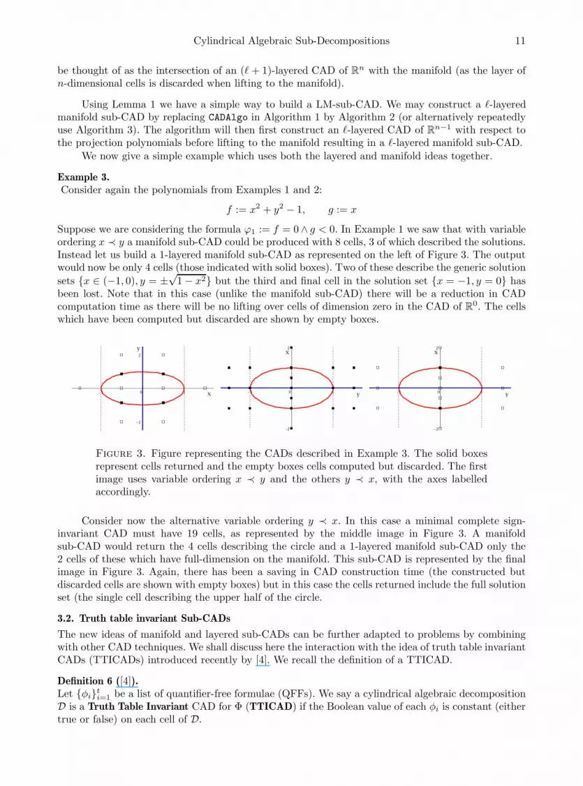
Suppose we are considering the formula ϕ1 := f = 0∧ g < 0. In Example 1 we saw that with variableordering x ≺ y a manifold sub-CAD could be produced with 8 cells, 3 of which described the solutions.Instead let us build a 1-layered manifold sub-CAD as represented on the left of Figure 3. The outputwould now be only 4 cells (those indicated with solid boxes). Two of these describe the generic solution

sets {x ∈ (−1, 0), y = ±√1− x2} but the third and final cell in the solution set {x = −1, y = 0} has

been lost. Note that in this case (unlike the manifold sub-CAD) there will be a reduction in CADcomputation time as there will be no lifting over cells of dimension zero in the CAD of R0. The cellswhich have been computed but discarded are shown by empty boxes.

Figure 3. Figure representing the CADs described in Example 3. The solid boxesrepresent cells returned and the empty boxes cells computed but discarded. The firstimage uses variable ordering x ≺ y and the others y ≺ x, with the axes labelledaccordingly.

Consider now the alternative variable ordering y ≺ x. In this case a minimal complete sign-invariant CAD must have 19 cells, as represented by the middle image in Figure 3. A manifoldsub-CAD would return the 4 cells describing the circle and a 1-layered manifold sub-CAD only the2 cells of these which have full-dimension on the manifold. This sub-CAD is represented by the finalimage in Figure 3. Again, there has been a saving in CAD construction time (the constructed butdiscarded cells are shown with empty boxes) but in this case the cells returned include the full solutionset (the single cell describing the upper half of the circle.

3.2. Truth table invariant Sub-CADs

The new ideas of manifold and layered sub-CADs can be further adapted to problems by combiningwith other CAD techniques. We shall discuss here the interaction with the idea of truth table invariantCADs (TTICADs) introduced recently by [4]. We recall the definition of a TTICAD.

Definition 6 ([4]).Let {φi}ti=1 be a list of quantifier-free formulae (QFFs). We say a cylindrical algebraic decompositionD is a Truth Table Invariant CAD for Φ (TTICAD) if the Boolean value of each φi is constant (eithertrue or false) on each cell of D.

12 D. J. Wilson, R. J. Bradford, J. H. Davenport and M. England

It was shown in [4] that truth table invariance is a very useful and important concept. Givena problem defined by a parent formula Φ built by a boolean combination of {φi}ti=1, a TTICAD issufficient and more efficient than either a sign-invariant CAD for all the polynomials or a CAD builtusing the theory of equational constraints (when applicable). Further, there are classes of problemsfor which a TTICAD is exactly the desired structure, such as the problem of decomposing a complexdomain according to the branch cuts of multivariate functions [3, 34, 23].

In [4] an algorithm was given for when each φi contains an explicit equational constraint. This hasrecently been extended to allow for φi’s without an equational constraint [22], but for ease of expositionwe will consider only the original algorithm. The algorithm involves a new projection operator whichencapsulates the interaction between the equational constraints of the φi’s whilst ignoring interactionsbetween polynomials that have no effect on the truth value of φi.

In the case where there is a parent formula Φ and all the φi have their own equational constraintwe can create a M-sub-TTICAD. We would use Algorithm 1 replacing ProjOp by the TTICADprojection operator in A and using a GenerateStack algorithm which checks for the necessary well-orientedness properties of TTICAD. The equational constraint set will contain all the equationalconstraints for the individual φi’s. Their product is an implicit equational constraint for the wholeformula and the sub-CAD produced will be for the manifold this product defines. We note thatalthough the manifold considered is that of the implicit equational constraint the TTICAD projectiontheory is more efficient that the equational constraint theory applied to this case (as described in [4]).

Creating layered TTICADs L-sub-TTICAD is also possible, again by adapting Algorithms 2 and3 with the TTICAD projection operator and appropriate GenerateStack algorithm. (See the technicalreport [41] for some further details and examples.)

Further, we can combine the ideas of Section 3.1 with TTICAD to produce layered manifoldsub-TTICADs.

Definition 7.Let {φi}ti=1 be a list of QFFs with each φi having equational constraint fi ∈ Q[x1, . . . , xn] with mainvariable xn. Let 1 ≤ ℓ ≤ n. A sub-CAD of a TTICAD for {φi}ti=1 containing all cells of dimension

n − 1 − i for 0 ≤ i < ℓ resting on the manifold defined by∏t

i=1 fi = 0 is called a Layered ManifoldSub-TTICAD (LM-sub-TTICAD).

Remark 3.As with ML-sub-CADs, a ℓ-layered manifold sub-TTICAD consists of the top ℓ-layers of cells on the

manifold∏t

i=1 fi = 0. Again, this can be thought of as the intersection of an (ℓ+ 1)-layered CAD ofRn with the manifold (as the layer of n-dimensional cells is discarded when lifting to the manifold).

We can construct LM-sub-TTICADs by using Algorithm 1 and substituting the TTICAD pro-jection operator for ProjOp and the layered TTICAD algorithm for CADAlgo. Example 5 in Section 5demonstrates the use of a LM-sub-TTICAD and the benefits of choosing to do so.

4. Complexity analysis

We provide a complexity analysis of the algorithms to compute sign-invariant manifold sub-CADs and1-layered manifold sub-CADs. We need to study three parts of the complexity:

Projection. The complexity of the equational constraint projection set needs to be analysed. Inparticular the number of polynomials, the maximum degree and size of their coefficients.

Calculation of (n− 1) dimension CAD. These values then can be used to estimate the complexityof the (n− 1)–dimensional CAD.

Lifting. Finally the complexity of the lifting stage can be combined with the previous step todescribe the complexity of the manifold CAD.

We recall the previous comprehensive work on CAD complexity by Collins [14] and McCallum[28].

Cylindrical Algebraic Sub-Decompositions 13

We first standardise some notation for a CAD with respect to a set of polynomials A: let n bethe number of variables, m the number of polynomials in A, d the maximum degree in any variableof the polynomials in A, and l the maximum norm length of the polynomials in A (where the normlength, |f |1, is the sum of the absolute values of the integer coefficients of a polynomial).

Let A1 := A and let Ai+1 = Proj(Ai). In general the projection operator used will be clear; mostof the following complexity analysis is with respect to Collins’ projection operator and, therefore, is a‘worst case scenario’ compared to the improved operators of McCallum [30] and Brown [6]. Let mk bethe number of polynomials in Ak, dk the maximum degree of Ak, and lk the maximum norm length.

4.1. Collins’ algorithm

Collins [14] works through the original CAD algorithm in great detail to analyse the complexity, andthis methodology is followed in [28]; we will recall some key results. These could all be uniformlyimproved with ideas from papers such as [12, 16], but that is not the aim of this paper.

In the projection stage we can bound the properties of the projection sets as follows:

mk ≤ (2d)3k

m2k−1

; dk ≤1

2(2d)2

k−1

; lk ≤ (2d)2k

l.

Combining these bounds gives us an idea of the projection phase. Collins shows that it is dominatedby

(2d)3n+1

m2n l2.

The base case and lifting algorithm requires the isolation of real roots of univariate polynomials.Collins bounds this procedure as follows. Let A be a set of univariate polynomials with degree bounded

by d and norm length bounded by l. Then for a given f ∈ A with d := deg(f) and l := |f |1 we canlower bound the distance between two roots by

1

2

(√ed

32 l)−d

. (1)

Collins uses his analysis of Heindel’s algorithm for real root isolation to show that isolating theroots is dominated by

d8 + d7 l3. (2)

Therefore the operations needed to isolate all roots in A, with m := |A|, is dominated by:

md8 +md7l3. (3)

For a given h, refining a root interval to 2−h is dominated by d2h3 + d2l2h. Collins multiplies allpolynomials in A and uses (1) to show that all roots are separated by:

δ :=1

2

(√e(md)

32 lm

)−md

.

If we take h to be log(δ) we can refine all intervals of the polynomials in

md(d2(m2dl +md log(md))3 +md3l3) = O(m7d7l3 +m2d4l3).

Combining this with (3) tells us that the necessary refinement of intervals for all the polynomials isdominated to

md8 +m7d7l3. (4)

Collins uses (4) along with the size of the full projection set to show that the base phase isdominated by

(2d)3n+3

m2n+2

l3.

We also need to consider the polynomials involved in the lifting stage. This involves lookingat the univariate polynomials created after substituting sample points, along with the polynomialsrequired to define the algebraic extensions of Q that the sample points are contained in.

We follow [14, 28] in using primitive elements to calculate the costs of operations, even thoughimplementers are extremely unlikely to use them. For each sample point β = (β1, . . . , βk) ∈ Rk thereis a real algebraic number α ∈ R such that Q(β1, . . . , βk) = Q(α). Let Aα be the polynomial in Q[x]

14 D. J. Wilson, R. J. Bradford, J. H. Davenport and M. England

defining α, that is A(α) = 0, along with an isolating interval Iα. Let d∗k be the maximum degree ofthese Aα, and l∗k the maximum norm length. Each coordinate βi is represented in Q(α) by anotherpolynomial, and let l′k be the maximum norm length of these polynomials. Then

d∗k ≤ (2d)22n−1

; l∗k, l′k ≤ (2d2)2

2n+3

m2n+1

l.

Let uk be the number of univariate cells (after substitution) and ck the number of cells at levelk. Then

uk, ck ≤ 22n

n∏

i=1

midi; and uk, ck ≤ (2d)3n+1

m2n . (5)

Finally, Collins combines all these results to give a complexity bound for the full algorithm. TheCollins Algorithm is dominated by

(2d)4n+4

m2n+6

l3. (6)

4.2. McCallum’s Cadmd algorithm

In [28], McCallum gives a complexity bound, using the same methodology as [14], for his Cadmd

algorithm which produces a 1-layered CAD. Thanks to the avoidance of algebraic numbers (all samplepoints in a 1-layered CAD can be produced directly in Q) the exponents are lower than in (6). Thecomplexity is dominated by

(2d)3n+4

m2n+4

l3. (7)

4.3. Analysis of PE(A) and (n− 1)-dimensional CADs

To have an accurate complexity we must consider some properties of the projection set: the size,maximum degree, and maximum norm length. Let E be the subset of A containing the factors of thedesignated equational constraint. Let mA := |A|, mE := |E|, mA\E := |A \ E|, and let dA, dE , dA\E ,lA, lE , and lA\E be defined similarly.

When constructing a CAD with respect to equational constraints, we use a projection operator,PE(A), defined by McCallum [31]:

PE(A) := P (E) ∪ {resxn(f, g) | f ∈ E, g ∈ A \ E}

where P (E) is an application of the operator as defined in [30]: the coefficients, discriminants andresultants of E. We will denote the resultant set, PE(A) \ P (E), by ResSetE(A).

The size of P (E) is bounded by the number of coefficients (mEdE), discriminants (mE), and

resultants ((

mE

2

)

= mE(mE−1)2 ). Therefore we have

|PE(A)| ≤ mEdE +mE +mE(mE − 1)

2+mEmA\E

=mE

2

(

2dE + 2mA\E +mE − 1)

=mE

2

(

2dE +mA\E +mA − 1)

. (8)

The maximum degree of PE(A) is the greater of the maximum degrees of P (E) and the resultantset. We also have a bound on the degree of a resultant with respect to x:

deg(resx(f, g)) ≤ (degx f + degx g) · (max(degy f, degy g)).

Using our overall degree bounds gives

maxdeg(ResSetE(A)) ≤ (dE + dA\E) ·max(dE , dA\E)

= max(d2E + dEdA\E , d2A\E + dEdA\E)

≤ max(2d2E , 2d2A\E). (9)

We also have

maxdeg(P (E)) ≤ max(dE , 2d2E, 2d

2E) = 2d2E . (10)

Cylindrical Algebraic Sub-Decompositions 15

Combining (9) and (10) gives a degree bound for PE(A)

max deg(PE(A)) ≤ max(2d2E , 2d2A\E) ≤ d2A. (11)

Finally, if we denote the maximum norm length of PE(A) by l, then we know l ≤ l2 (as PE(A) ≤Proj(A)) so

l ≤ l2 ≤ (2dA)22 lA = 16d4AlA. (12)

Using the bounds from (8), (11) and (12) to substitute into (6) and (7) to get estimates forthe complexity of the (n − 1)-dimensional CAD. The complexity of a complete (n − 1)-dimensionalPE(A)-invariant Collins CAD is dominated by

≤(

2 · 2d2A)22(n−1)+8

(

mE(2dE +mA +mA\E − 1)

2

)2n−1+6

(

16d4AlA)3

≤ 163(

4d2A)22n+6

(

mE(2dE + 2mA − 1)

2

)2n+5

l3Ad12A . (13)

The complexity of a 1-layered (n− 1)-dimensional PE(A)-invariant McCallum CAD is dominated by

≤(

2 · 2d2A)3n−1+4

(

mE(2dE +mA +mA\E − 1)

2

)2n−1+4

(

16d4AlA)3

≤ 163(

4d2A)3n+3

(

mE(2dE + 2mA − 1)

2

)2n+3

l3Ad12A . (14)

4.4. Overall complexities

So far, we have computed the complexities of the (n− 1)-dimensional CADs. The final step is to liftover these cells with respect to the equational constraints. From (5) we can bound the number ofunivariate polynomials and so know from (4) the isolations will be dominated by:

(2dE)3n+1

m2n

E d8E +(

(2dE)3n+1

m2n

E

)7

d7E l3E. (15)

By combining (15) with (13) and (14) we are now in a position to describe the overall complexitiesof our manifold algorithms. Note that (15) will be a large overestimation for the 1-layered case butwill be sufficient for our purposes.

Theorem 2.The complexity for computing a manifold CAD using Collins’ algorithm is dominated by:

212(

22d2A)4

n+3

(

mE(2dE + 2mA − 1)

2

)2n+5

l3Ad12A +

(2dE)3n+1

m2n

E d8E +(

(2dE)3n+1

m2n

E

)7

d7E l3E . (16)

The complexity for computing a 1-layered manifold sub-CAD is dominated by:

212(

22d2A)3

n+3

(

mE(2dE + 2mA − 1)

2

)2n+3

l3Ad12A +

(2dE)3n+1

m2n

E d8E +(

(2dE)3n+1

m2n

E

)7

d7E l3E , (17)

where we have used bold face to indicate the key dfferences in the exponents.

16 D. J. Wilson, R. J. Bradford, J. H. Davenport and M. England

n dA dE mA mE mA\E lA lE CAD M-CAD 1-L CAD 1-L M-CAD

2 2 2 3 1 2 2 2 102589 101318 10470 10319

2 3 2 3 1 2 2 2 103310 101680 10598 10407

3 4 3 5 2 3 3 2 1015155 107695 102065 101400

5 5 4 7 3 4 4 3 10263876 10132551 1020117 1013502

1 3 2 3 1 2 2 2 10858 10447 10205 10145

2 3 2 3 1 2 2 2 103310 101680 10598 10407

3 3 2 3 1 2 2 2 1012994 106538 101763 101183

4 3 2 3 1 2 2 2 1051486 1025816 105228 103490

5 3 2 3 1 2 2 2 10204965 10102620 1015561 1010375

6 3 2 3 1 2 2 2 10817905 10409218 1046438 1030951

7 3 2 3 1 2 2 2 103267712 101634377 10138825 1092524

Table 1. The size of complexity estimates for CAD algorithms with various param-eter choices.

Figure 4. The double logarithm of the complexities of the algorithms with dA = 3,dE = 2, mA = 3, mE = 1, mA\E = 2, lA = 2, lE = 2 and n varying from 1 to 5. Fromtop to bottom the lines represent the algorithms as listed in Table 1.

4.5. Comparison of complexities

In Theorem 2 we have emboldened the exponents to highlight the difference between (16) and (17),but it can be difficult to visualise the comparison. Therefore we offer computations for the scale ofthe complexities for sample parameter sets. These are shown in Table 1. For each set of parametersgiven we provide the complexity estimates for a CAD of Rn (CAD), an M-CAD of Rn (M-CAD), a1-layered CAD of Rn (1-L CAD), and a 1-layered manifold sub-CAD of Rn (1-L M-CAD).

To visualise how the coefficient of n in the double exponential has changed, we plot the doublelogarithm of the complexities for parameters dA = 3, dE = 2, mA = 3, mE = 1, mA\E = 2, lA = 2,lE = 2 whilst n varies from 1 to 5. This is shown in Figure 4. The diagram shows visibly the dropin the constant in the exponents of (16) and (17), but the scaling factor of the exponent remains thesame between manifold and non-manifold versions of each algorithm.

Cylindrical Algebraic Sub-Decompositions 17

Figure 5. Intersection of the three surfaces from Example 4. The red surface (thedarkest in black and white) is the equational constraint.

5. Examples and Implementation

The procedures described in this paper are all implemented in the Maple package ProjectionCAD

[21, 22], within the subpackages ManifoldCAD and LayeredCAD. More details of the implementationof layered CAD are given in [41].

All experiments were run on a Linux desktop (3.1GHz Intel processor, 8.0Gb total memory) withMaple 16 (command line interface) and Qepcad-B 1.69. For Qepcad the options +N500000000 and+L200000 were provided and the initialisation included in the timings.

We provide some demonstrative examples showing how LM-sub-CAD and LM-sub-TTICAD areuseful for studying problems.

5.1. Example using 1-layered manifold sub-CAD

Example 4.Assume variable ordering x ≻ y ≻ z and consider the following formula involving 3 random polyno-mials of degree 2 (generated using Maple’s randpoly function):

Φ := −50xy + 56yz + 41z2 + 67x− 55y − 21 = 0

∧ 36xy + 76xz − 58yz + 69z2 + 75y + 27 > 0

∧ −55x2 + 10xy − 88x+ 80y + z − 39 > 0.

We wish to describe the valid regions of R3 in which Φ is satisfied. As can be seen in Figure 5, there aremultiple intersections and, importantly, a lot of interaction between the two non-equational constraintsaway from the manifold defined by the equational constraint. This suggests that M-sub-CAD couldbe beneficial. Further, if only generic solution sets are of interest then a 1-layered manifold sub-CADcould offer further savings.

To solve the problem we construct a variety of CADs and sub-CADs with the results shown below.MapleCAD refers to the the algorithm to produce sign-invariant CADs via triangular decompositionbuilt into Maple [13] and Qepcad the default use of Qepcad-B to build a partial CAD [7]. Theother algorithms are all implemented in our Maple package ProjectionCAD [22]: CADFull buildsa sign-invariant CAD, ECCAD a CAD invariant with respect to an equational constraint, and the

18 D. J. Wilson, R. J. Bradford, J. H. Davenport and M. England

final three algorithms are those described in this paper applied with the same projection operator asECCAD.

MapleCAD. 9841 cells, 1085.109 seconds.CADFull. 16993 cells, 2544.688 seconds.Qepcad. 17047 cells, 385.679 seconds.ECCAD. 1315 cells, 19.172 seconds.Manifold sub-CAD. 422 cells, 17.421 seconds.2-Layered Manifold Sub-CAD. 348 cells, 15.626 seconds.1-Layered Manifold Sub-CAD. 138 cells, 3.625 seconds.

As can be clearly seen, making use of the equational constraint dramatically reduces the com-putation involved. A manifold sub-CAD further reduces the size of the output which will lead to timesavings on any future work. Indeed, Qepcad evaluates Φ on each cell in the process of constructing anequivalent quantifier-free formula (in this case, Φ cannot be simplified). Of the 17047 cells constructed,Φ is only valid on 290 of them. The 16757 false cells that are constructed and on which Φ is evaluatedwill be a significant contribution to the computation time, (other factors will be the improved liftingperformed by ECCAD as described in [22]).

If we are concerned only with finding the generic solution sets rather than all solutions then a1-layered manifold sub-CAD may be used offering further time-savings. This replaces an output ofaround 17,000 cells which took 45 minutes to compute with another of only 138 cells computed in lessthan 4 seconds. If solutions of lower dimension are also needed then the 2-layered manifold sub-CAD(348 cells) or the complete manifold sub-CAD (422 cells) can be used instead.

We can evaluate Φ on all the cells produced in the 1-LM-sub-CAD almost instantly to find thatthere are 36 cells on which Φ is satisfied (although the equation is by definition true for all of themthe other constraints vary). The space described by these cells differ only from the space described bythe 290 valid cells of Qepcad by cells of dimension 1 and 0. Whilst not defining all possible solutions,those missed are of measure zero and may not be needed to solve the problem at hand.

In general, a 1-layered manifold sub-CAD can be used to find the generic solutions (those differingonly by a set of measure zero from the full-solution set) for any problem of the form f = 0 ∧ Ψ(gi)where f = 0 defines a manifold of real co-dimension 1 and Ψ is a quantifier-free formula involving onlystrict inequalities for the gi. In general, we may find that there are no solutions of full dimension onthe manifold, and can use the recursive approach for layered CAD to incrementally build extra layersas required.

5.2. Example using 1-layered manifold sub-TTICAD

We now consider a problem suitable for using a combination of our new sub-CAD ideas and TTICAD.

Example 5.Let us define the following quantifier free formulae:

ϕ1 := x2 + y2 + z2 = 1 ∧ xy + yz + zx < 1 ∧ x3 − y3 − z3 < 0, (18)

ϕ2 := (x− 1)2 + (y − 1)2 + (z − 1)2 = 1 ∧ (x− 1)(y − 1) + (y − 1)(z − 1)+

(z − 1)(x− 1) < 1 ∧ (x− 1)3 − (y − 1)3 − (z − 1)3 < 0. (19)

The surfaces defined by the polynomials in ϕ1 are shown in Figure 6, while those in ϕ2 are the samebut shifted.

Assume the variable ordering x ≻ y ≻ z and consider the problem of finding all regions of R3

satisfying the following formula:Φ := ϕ1 ∨ ϕ2. (20)

We can attack this problem naıvely and input the 6 polynomials in Φ to a CAD algorithm. Leavingeither Maple’s RegularChains CAD implementation or our ProjectionCAD implementation runningfor 72 hours fails to produce a CAD, while using Qepcad results in a “prime list exhausted” error (amemory constraint) after two hours.

Cylindrical Algebraic Sub-Decompositions 19

Figure 6. Intersection of the surfaces from ϕ1 in Example 5 – the sphere defined bythe equational constraint is in red (the darkest surface in black and white).

We can explicitly tell Qepcad to utilise the implicit equational constraint (the product of thetwo equations) and then obtain a CAD with 6165 cells in 35304.364 seconds (around 10 hours). Thisproblem is well suited for TTICAD and applying the ProjectionCAD implementation on the twoformulae ϕ1 and ϕ2 produces 4861 cells in 608 seconds.

We now consider how a 1-Layered Manifold Sub-TTICAD may be constructed. Each formulaϕi contains an equational constraint, and so can only be true on the manifold it defines. Thereforewe may first project using the TTICAD operator applied to ϕ1 and ϕ2 and construct a 1-layeredsub-CAD of R2 with respect to this projection set. This takes 573 seconds and produces 249 cells inR2. We then lift with respect to both of the equational constraints onto the manifold defined by theirproduct. This takes a further 2 seconds and produces 528 2-dimensional cells on the 2-dimensionalmanifold in R3. Whilst there is only a 5% saving in time from TTICAD, there is a 89% saving incells. If we then evaluate Φ on each cell we can identify the cells of full dimension (with respect to themanifold) where Φ is valid. Any other cells on which Φ is true would have to be of lower dimension,and so a 1-layered manifold sub-TTICAD is sufficient up to a set of measure zero.

If solutions of lower dimension are needed then we can also produce a 2-layered manifold sub-TTICAD and the full manifold sub-TTICAD which contain 1514 cells and 1976 cells, respectively.Both take under 10 minutes to construct (quicker than constructing the full TTICAD). Note also thatover half the cells produced in a complete TTICAD do not lie on either of the manifolds defined bythe equational constraints of ϕ1 and ϕ2.

To magnify the issues displayed here consider a third formula formed by a different shift of theoriginal surfaces:

ϕ3 := (x+ 1)2 + (y + 1)2 + (z + 1)2 = 1 ∧ (x+ 1)(y + 1) + (y + 1)(z + 1)+

(z + 1)(x+ 1) < 1 ∧ (x+ 1)3 − (y + 1)3 − (z + 1)3 < 0. (21)

We combine with Φ to form a new overall formula:

Φ∗ := ϕ1 ∨ ϕ2 ∨ ϕ3. (22)

20 D. J. Wilson, R. J. Bradford, J. H. Davenport and M. England

Given the above results for Φ it would be foolish to attempt to solve this problem withoututilising the presence of the equational constraints. We repeat the approach used for Φ. This timethe 1-layered sub-CAD of R2 takes 3200.389 seconds (just under an hour) and produces 488 cells.It takes a further 7.250 seconds to construct the 1-layered manifold sub-TTICAD, resulting in 1096cells. Attempting to construct a sign-invariant CAD is not going to be feasible, but we can constructa TTICAD. This takes 4488.764 seconds (an hour and a quarter) and produces 10033 cells; nearly 10times the number of cells a 1-layered manifold sub-TTICAD has. Although the TTICAD will containall valid cells for Φ, the 1-layered manifold sub-TTICAD will provide descriptions of general familiesof solutions.

If solutions of lower dimensions are needed then a 2-layered manifold sub-TTICAD or the com-plete manifold sub-TTICAD can be constructed. A 2-layered manifold sub-TTICAD contains 3153cells, whilst the manifold sub-TTICAD contains 4117 cells. This again highlights the fact that overhalf the cells produced in the TTICAD do not satisfy any of the equational constraints and are thusunnecessary to describe the solution.

5.3. A piano movers’ problem

An application of CAD of great interest is motion planning. Given a semi-algebraic object, an initialand desired position, and semi-algebraic obstacles, a CAD can be constructed of the valid configurationspace of the object. The connectivity of this space can then be used to determine if a feasible pathfrom the initial position of the object to the desired endpoint is possible.

A well-studied problem in this area is the movement of a ladder through a right-angled corridor,as proposed in [17]. The problem consists of a ladder of length 3 inside a right-angled corridor of width1 with the aim of moving from from position 1 to position 2 in Figure 7.

1

2

Figure 7. The piano movers problem considered in [17]

Although in 2-dimensional real space the problem lies in a 4-dimensional configuration spacewhich makes it far more difficult to describe with a CAD. It is still not feasible to build a CAD forthe formulation of the problem given in [17] but recently progress was made in [40] by reformulatingthe problem. We can now construct a CAD of the configuration space using Qepcad with 285,419cells in around 5 hours (without Qepcad’s partial CAD techniques this increases to 1,691,473 cellsand over 24 hours computation time). A representation of the 2-dimensional CAD produced on routeto the full 4-dimensional CAD is given in Figure 8.

The formulation of the ladder includes an explicit equational constraint. Denoting the endpointsof the ladder as (x, y) and (x′, y′), the length of the ladder becomes the equational constraint:

(x − x′)2 + (y − y′)2 = 9.

The problem is therefore suited to treatment with a M-sub-CAD. Indeed, we can see from Figure 8that there is a great deal of information computed which is of no use in describing the suitable paths.It would be of great use if partial CAD techniques can be adapted to restrict a CAD or sub-CAD toa sub-CAD of just the corridor highlighted.

Cylindrical Algebraic Sub-Decompositions 21

Figure 8. A representation of the 2-dimensional induced CAD produced for the newformulation of the piano movers problem in [40].

Within this three-dimensional manifold (embedded within R4) the important cells are those thatare three-dimensional. This is as cells of lesser dimension correspond to physically infeasible situations(i.e. one dimensional subspaces of R2). Therefore a LM-sub-CAD could be used as an overview of theproblem.

Constructing the 1-layered sub-CAD of R3 produces 64,764 cells in around four and a half hours,and lifting to the manifold takes a further 15 minutes and produces 101,924 cells. This is a saving(both in terms of cells and timing) on the partial CAD produced by Qepcad. Adjacency informationwill have to be computed for a full solution to the problem (which will possibly require a 2-layeredmanifold sub-CAD) and thus any savings in cells will be of huge advantage to the feasibility of thesecomputations.

6. Conclusions and further work

We have formalised the idea of a cylindrical algebraic sub-decomposition. Whilst a simple idea, itcan be hugely powerful and the examples presented show that massive cell reductions are possible.The time reductions in computing the CADs are less dramatic, but since most problems using CADwill require some further computation on the cells (such as polynomial evaluation) the overall timesavings will be much greater. Applications involving complicated calculation on the cells will benefiteven more. For example, the calculation of adjacency information for use in motion planning or theevaluation of multi-valued functions at possibly algebraic sample points for branch cut analysis.

We provided examples of sub-CADs in the literature, along with two new concepts (and algo-rithms to produce them): manifold sub-CADs and layered sub-CADs. While each has its own interest,we find that savings may be magnified through the interaction between different concepts. We providedexamples of this involving layered manifold sub-CADs, manifold sub-TTICADs and layered manifoldsub-TTICADs This final type of sub-CAD can be used to partially solve problems having a particular

22 D. J. Wilson, R. J. Bradford, J. H. Davenport and M. England

structure, identifying large regions of valid cells, and it was shown this enables us to tackle problemspreviously infeasible.

There is great scope for future work with some important questions we are working on as follows.

• Can we identify classes of problems where a layered manifold sub-CAD or sub-TTICAD is suffi-cient to entirely solve a problem?• How the interaction of the layered and manifold theories should be implemented when the poly-nomials defining the manifold do not contain xn.• How best to adapt existing techniques (such as partial CAD) to output sub-CADs.• Can we develop heuristics (or adapt existing ones [20, 5]) on when and how we should use whichtheories?• Can we keep track of where cells arise when constructing a manifold sub-TTICAD so that overeach cell we lift only to the manifolds for relevant φi? This can be thought of as an analogue ofpartial CAD for TTICAD. This may alter the output significantly (it may not be a sub-CAD ofa CAD that can be constructed by current technology) but could allow for even smaller outputfor given problems.• Can we parallelise the algorithms? The idea mentioned in [29] of lifting over sets of cells inde-pendently could be generalised. (Preprocessing CAD problems to allow for parallelisation wasdiscussed in [27] but this involved only the boolean logic of the problem).

There are also many interesting questions arising from whether certain properties of CADs transferover to their sub-CADs. For example, any existing adjacency algorithms require CADs to be particu-larly ‘well-behaved’, and it may be possible to avoid problematic cells through sub-CADs, extendingthe use of such algorithms. The idea of a well-oriented CAD needed for many modern CAD algorithms[30, 6] may also be problematic on a CAD, but not an issue on certain sub-CADs. These ideas needfurther investigation.

An overarching aim is to develop a general CAD framework which would allow for identificationof when certain kinds of sub-CADs should be used, automatically combining appropriate methodswhen possible and making choices automatically when required based on heuristic information. Thiswould identify, for a given problem, an efficient way to produce a φ-sufficient sub-CAD and thusdescribe the solution set.

Acknowledgements

This work was supported by the EPSRC grant: EP/J003247/1. The authors would also like to thankProfessor Gregory Sankaran for his thoughts and feedback on the topic, and Professor Scott McCallumfor many stimulating conversations on TTICAD.

References

[1] D. Arnon, G.E. Collins, and S. McCallum. Cylindrical algebraic decomposition I: The basic algorithm.SIAM J, Comput., 13:865–877, 1984.

[2] J. Backelin. Square multiples n give infinitely many cyclic n-roots. Matematiska Institutionen reportsseries, Stockholms Universitet, 1989.

[3] R. Bradford and J.H. Davenport. Towards better simplification of elementary functions. In Proceedings ofthe 2002 international symposium on symbolic and algebraic computation, ISSAC ’02, pages 16–22. ACM,2002.

[4] R. Bradford, J.H. Davenport, M. England, S. McCallum, and D. Wilson. Cylindrical algebraic decompo-sitions for boolean combinations. In Proceedings of the 38th International Symposium on Symbolic andAlgebraic Computation, ISSAC ’13, pages 125–132. ACM, 2013.

[5] R. Bradford, J.H. Davenport, M. England, and D. Wilson. Optimising problem formulations for cylindricalalgebraic decomposition. In J. Carette, D. Aspinall, C. Lange, P. Sojka, and W. Windsteiger, editors,

Cylindrical Algebraic Sub-Decompositions 23

Intelligent Computer Mathematics, volume 7961 of Lecture Notes in Computer Science, pages 19–34.Springer Berlin Heidelberg, 2013.

[6] C.W. Brown. Improved projection for cylindrical algebraic decomposition. J. Symb. Comput., 32(5):447–465, 2001.

[7] C.W. Brown. An overview of QEPCAD B: a tool for real quantifier elimination and formula simplification.Journal of Japan Society for Symbolic and Algebraic Computation, 10(1):13–22, 2003.

[8] C.W. Brown. The McCallum projection, lifting, and order-invariance. Technical report, U.S. Naval Acad-emy, Computer Science Department, 2005.

[9] C.W. Brown. Constructing a single open cell in a cylindrical algebraic decomposition. In Proceedings ofthe 38th International Symposium on Symbolic and Algebraic Computation, ISSAC ’13, pages 133–140.ACM, 2013.

[10] C.W. Brown and J.H. Davenport. The complexity of quantifier elimination and cylindrical algebraic de-composition. In Proceedings of the 2007 international symposium on Symbolic and algebraic computation,ISSAC ’07, pages 54–60. ACM, 2007.

[11] C.W. Brown, M. El Kahoui, D. Novotni, and A. Weber. Algorithmic methods for investigating equilibriain epidemic modelling. J. Symbolic Computation, 41:1157–1173, 2006.

[12] M.A. Burr. Applications of continuous amortization to bisection-based root isolation. Preprint:http: // arxiv. org/ abs/ 1309. 5991 , 2013.

[13] C. Chen, M. Moreno Maza, B. Xia, and L. Yang. Computing cylindrical algebraic decomposition viatriangular decomposition. In Proceedings of the 2009 international symposium on Symbolic and algebraiccomputation, ISSAC ’09, pages 95–102. ACM, 2009.

[14] G.E. Collins. Quantifier elimination for real closed fields by cylindrical algebraic decomposition. In Pro-ceedings of the 2nd GI Conference on Automata Theory and Formal Languages, pages 134–183. Springer-Verlag, 1975.

[15] G.E. Collins and H. Hong. Partial cylindrical algebraic decomposition for quantifier elimination. J. Symb.Comput., 12:299–328, 1991.

[16] J.H. Davenport. Computer algebra for cylindrical algebraic decomposition. Technical Report TRITA-NA-8511, NADA KTH Stockholm. Reissued as Bath Computer Science Technical report 88-10. Available athttp://staff.bath.ac.uk/masjhd/TRITA.pdf, 1985.

[17] J.H. Davenport. A “Piano-Movers” Problem. SIGSAM Bull., 20(1-2):15–17, 1986.

[18] J.H. Davenport, R. Bradford, M. England, and D. Wilson. Program verification in the presence of complexnumbers, functions with branch cuts etc. In 14th International Symposium on Symbolic and NumericAlgorithms for Scientific Computing, SYNASC ’12, pages 83–88. IEEE, 2012.

[19] J.H. Davenport and J. Heintz. Real quantifier elimination is doubly exponential. J. Symb. Comput., 5(1-2):29–35, 1988.

[20] A. Dolzmann, A. Seidl, and T. Sturm. Efficient projection orders for CAD. In Proceedings of the 2004international symposium on Symbolic and algebraic computation, ISSAC ’04, pages 111–118. ACM, 2004.

[21] M. England. An implementation of CAD in Maple utilising McCallum projection. Depart-ment of Computer Science Technical Report series 2013-02, University of Bath. Available athttp://opus.bath.ac.uk/33180/, 2013.

[22] M. England. An implementation of CAD in maple utilising problem formulation, equational constraintsand truth-table invariance. Department of Computer Science Technical Report series 2013-04, Universityof Bath. Available at http://opus.bath.ac.uk/35636/, 2013.

[23] M. England, R. Bradford, J.H. Davenport, and D. Wilson. Understanding branch cuts of expressions. InJ. Carette, D. Aspinall, C. Lange, P. Sojka, and W. Windsteiger, editors, Intelligent Computer Mathe-matics, volume 7961 of Lecture Notes in Computer Science, pages 136–151. Springer Berlin Heidelberg,2013.

[24] I.A. Fotiou, P.A. Parrilo, and M. Morari. Nonlinear parametric optimization using cylindrical algebraicdecomposition. In Decision and Control, 2005 European Control Conference. CDC-ECC ’05., pages 3735–3740, 2005.

24 D. J. Wilson, R. J. Bradford, J. H. Davenport and M. England

[25] H. Hong. An improvement of the projection operator in cylindrical algebraic decomposition. In Proceedingsof the international symposium on Symbolic and algebraic computation, ISSAC ’90, pages 261–264. ACM,1990.

[26] H. Iwane, H. Yanami, H. Anai, and K. Yokoyama. An effective implementation of a symbolic-numericcylindrical algebraic decomposition for quantifier elimination. In Proceedings of the 2009 conference onSymbolic Numeric Computation, SNC ’09, pages 55–64, 2009.

[27] H.K. Malladi and A. Dukkipati. A preprocessor based on clause normal forms and virtual substitutions toparallelize cylindrical algebraic decomposition. Preprint: http: // arxiv. org/ abs/ 1112. 5352v3 , 2013.

[28] S. McCallum. Solving polynomial strict inequalities using cylindrical algebraic decomposition. The Com-puter Journal, 36(5):432–438, 1993.

[29] S. McCallum. A computer algebra approach to path finding in the plane. In J. Harland, editor, Proceedingsof Computing: The Australasian Theory Symposium (CATS), pages 44–50, 1997.

[30] S. McCallum. An improved projection operation for cylindrical algebraic decomposition. In B. Cavinessand J. Johnson, editors, Quantifier Elimination and Cylindrical Algebraic Decomposition, Texts & Mono-graphs in Symbolic Computation, pages 242–268. Springer-Verlag, 1998.

[31] S. McCallum. On projection in CAD-based quantifier elimination with equational constraint. In Pro-ceedings of the 1999 international symposium on Symbolic and algebraic computation, ISSAC ’99, pages145–149. ACM, 1999.

[32] S. McCallum. On propagation of equational constraints in CAD-based quantifier elimination. In Pro-ceedings of the 2001 international symposium on Symbolic and algebraic computation, ISSAC ’01, pages223–231. ACM, 2001.

[33] L.C. Paulson. Metitarski: Past and future. In L. Beringer and A. Felty, editors, Interactive TheoremProving, volume 7406 of Lecture Notes in Computer Science, pages 1–10. Springer, 2012.

[34] N. Phisanbut, R.J. Bradford, and J.H. Davenport. Geometry of branch cuts. ACM Communications inComputer Algebra, 44(3):132–135, 2010.

[35] J.T. Schwartz and M. Sharir. On the “Piano-Movers” Problem: II. General techniques for computingtopological properties of real algebraic manifolds. Adv. Appl. Math., 4:298–351, 1983.

[36] A. Seidl and T. Sturm. A generic projection operator for partial cylindrical algebraic decomposition.In Proceedings of the 2003 international symposium on Symbolic and algebraic computation, ISSAC ’03,pages 240–247. ACM, 2003.

[37] A. Strzebonski. Solving systems of strict polynomial inequalities. J. Symb. Comput., 29(3):471–480, 2000.

[38] A. Strzebonski. Cylindrical algebraic decomposition using validated numerics. Journal of Symbolic Com-putation, 41(9):1021–1038, 2006.

[39] A. Strzebonski. Solving polynomial systems over semialgebraic sets represented by cylindrical algebraicformulas. In Proceedings of the 2012 International Symposium on Symbolic and Algebraic Computation,ISSAC ’12, pages 335–342. ACM, 2012.

[40] D. Wilson, J.H. Davenport, M. England, and R. Bradford. A “piano movers” problem reformulated. In15th International Symposium on Symbolic and Numeric Algorithms for Scientific Computing, SYNASC’13. IEEE, 2013.

[41] D. Wilson and M. England. Layered cylindrical algebraic decomposition. Department of Computer ScienceTechnical Report series 2013-05, University of Bath. Available at http://opus.bath.ac.uk/36712/, 2013.

D. J. Wilson, R. J. Bradford, J. H. Davenport and M. EnglandDepartment of Computer Science, University of Bath, Bath, BA2 7AY, Englande-mail: {D.J.Wilson, R.J.Bradford, J.H.Davenport, M.England}@bath.ac.uk