An approximation for prey-predator models with time delay

N ELSEVIER Physica D 110 (1997) 313-322

PHYSICA B

An approximation for prey-predator models with time delay Jose Faro, Santiago Velasco *

Departamento de F[sica Aplicada, Universidad de Salamanca, 37008 Salamanca, Spain

Received 7 February 1997; received in revised form 6 May 1997; accepted 16 May 1997 Communicated by A.M. Albano

Abstract

A prototype prey-predator (P-D) model in which the effective size of the predator population interacting with its prey follows an instantaneous time-delay r regarding its total size is considered here. A simplified model was derived after substituting the approximation D(t - r) ,~ D(t) - r / ) ( t ) into the above time-delay model. In order to assess the reliability of the simplified model, we performed a comparative study of both models under a wide range of parameter values, focusing on the effect of r on two issues: (i) the boundary (in parameter space) between the regions leading either to stable fixed points or to limit cycles, and (ii) periods and amplitudes. We have found that, for small enough values of r compared with the period characteristic of the non-delay model, both the boundary and the periods and amplitudes obtained for the time-delay model can be fairly approximated by the corresponding results for the simplified model.

PACS: 02.30.Ks; 87.10.+e; 89.60.+x Keywords: Time delay; Population dynamics; Computer simulation; Ecological studies

1. Introduct ion

A major trend in theoretical work on prey-predator dynamics has been to derive more realistic models, trying to

keep to a minimum the unavoidable increase in the complexity of their mathematics. This effort has concentrated

mainly on the functional form of growth rates (for instance, making per capita growth rates to depend on both the prey

and predator densities to include some maximum carrying capacity [1], some uptake l imitation [1] or cannibalism

[2,3]), on incorporating spatial heterogeneities [4,5], as well as on including temporal fluctuations in environmental

and physiological parameters [6]. In contrast, the effect of t ime delays on the behavior of prey-predator ( P - D )

systems remains to a large extent quite unexplored.

Time delay plays an important role in many biological dynamical systems, being particularly relevant in ecology

[1], where time delays have been recognized to contribute critically to the stable or unstable outcome of prey

densities due to predation [7]. Time-delay models have been developed both for single species and for several

interacting species [8-11]. These models (both "continuously distributed" and "instantaneous" t ime-delay models)

* Corresponding author. Tel.: +34 23 29 44 36; fax: +34 23 29 45 84; e-mail: [email protected].

0167-2789/97/$17.00 Copyright © 1997 Elsevier Science B.V. All rights reserved PII S0167-2789(97)00124-3

314 J. Faro, S. Velasco/Physica D 110 (1997) 313-322

are, however, difficult to work with and to think about. This is particularly true for "instantaneous" time-delay models, which are less amenable to analytical study than models with "continuously distributed" time-delay, and for which (to our knowledge) there are less general results of practical relevance [9,10].

Recently [12], it has been demonstrated that the dynamics of a one-dimensional time-delay oscillator, 2(t) = - k x (t - 7:) (where the dot means derivation with respect to t and r is the time delay), can be fairly approximated by x(t - r) ~ x(t) - r2( t ) when T is such that r << I~T~ . We propose here that, under appropriate conditions, a similar approximation may be applied to prey-predator systems with time delay, rendering them more amenable to analytical and numerical study.

In this paper we consider a case model of a simple two species prey-predator model with time delay, rather than several related models. Lotka-Volterra equations are used [8,13] with some modifications, which consist of: (a) a logistic resource-limitation of the prey (carrying capacity), (b) an "appetite saturation" of the predator (uptake limitation), (c) an instantaneous time delay, r , in the response of predator to contacts with prey, which accounts for the time to

reach both reproductive and hunting maturity. We have simplified this time-delay model into an ODE model by substituting the approximation D (t - r) ~ D (t) --

/) (t) into the model's equations, and analyzed the extent to which this simplified model is a good approximation of the original, time-delay model. This was done by performing a comparative study of both models under a wide range of parameter values, focusing on the effect of r on: (i) the boundary (in parameter space) between the regions leading either to stable fixed points or to limit cycles, and (ii) periods and amplitudes in the oscillatory regime. We have found that, for small enough values of r compared with the period characteristic of the non-delay model, (i) the boundary for the time-delay model can be fairly approximated by the equivalent boundary for the simplified model, which can be calculated analytically; and (ii) the simplified model also reproduce very well the periods and amplitudes obtained numerically with the original model.

2. The model

Consider the following model:

~6( t )=aP( t ) ( 1 k ~ t ) ) bP( t )D( t ) - h + P ( t ) ' ( l a )

[ ~ ( t ) - ~P(t)D(t) dD(t) . (lb) h + P (t)

where P and D denote, respectively, the total number of individuals in the prey and predator populations, a is the growth rate of the prey, a / k the logistic growth limitation, b and ~ the prey-predator interaction constants, d the death rate of the predator, and h is the half saturation food uptake. Parameters a,/~, ~, d, k and h are positive real constants.

The first term in Eq. (1 a) models the growth rate of prey with resource limitation, with maximum carrying capacity a/k . The second term of this equation says that the rate at which prey are consumed at time t is, on the one side, limited by a maximum uptake per unit of predator (/~) and, on the other side, is determined by how many predators there are at time t. However, since the real thing is that prey are consumed at time t by the population of adult predator (i.e. predator individuals that have reached both reproductive and hunting maturity) present at time t, this last assumption probably is in many cases a too drastic simplification. The same apply to the first term of Eq. (lb), which models the growth rate of predator with uptake limitation. Therefore, denoting Da(t) the total number of adult predator at time t, a more correct version of model (1) is

J. Faro, S. Velasco/Physica D 110 (1997) 313-322 315

[~(t) = a P ( t ) (1 k P ( t ) bP(t)Da(t)h + P( t ) ' (2a)

D ( t ) - ~P( t )Da( t ) dD( t ) . (2b) h + P( t )

However, in principle this model is not a closed dynamical system for variables P and D, because of the presence of variable Da. Yet, this problem can be overcome by assuming that for newborn predator individuals it takes a time

to to reach the adult stage and that, because of this, the totality of adult predator at time t, Da(t), is constituted by

the surviving individuals (at this time t) from the total predator population at time t - to (i.e. D(t -- to)). The size of this surviving (adult) population can be easily calculated in terms of D(t - to) from the rate of predator decay, which is assumed to be - d D ( t ) (second term in Eq. (2b)). Thus, the cohort of D(t - to) individuals will decay with

this rate, so that at time t there would have survived

Da(t) = D(t -- to)e -dr° (3)

individuals (this is obtained by integrat ing/)( t ) ---- - d D ( t ) from t - to to t). Substituting Eq. (3) into system (2) leads to the following time-delay model (closed equation system for variables P and D):

[ ~ ( t ) = a P ( t ) ( 1 k P ( t ) ) bP(t)D(t-to)h + P( t ) ' (4a)

[~(t) = c P ( t ) D ( t - to) _ dD( t ) , (4b) h + P( t )

where b = /~e -at° (__ b) and c = ~e -dr° (<_ 2) are now effective prey-predator interaction parameters. This is

the time-delay case model that will be analyzed here. An implicit assumption of model (4) is that any reproductive delay in the prey population can safely be ignored.

In order to reduce the number of parameters, we non-dimensionalize the above model (4) by choosing a time scale based upon the growth rate of prey, a; thus, time will be normalized in units of 1/a, P in units of a / k and D in units of a2/bk (for simplicity, we denote the dimensionless variables also as t, P and D). Then the system (4)

simplifies into

P( t ) = P( t ) (1 - P(t ) )

D( t ) = q P ( t ) D ( t - r) H + P(t)

where

H = hk /a , q = c/a,

P ( t ) D ( t - ~)

H + P( t ) ==-- f l ( P ( t ) , D( t -- r)) ,

-- rD( t ) ---- f z ( P ( t ) , D( t ) , D( t - r)) ,

(5a)

(Sb)

r = d /a , T -= ato. (6)

3. The non-trivial steady state and stability

The values of the steady states of model (5) are determined analytically by setting f l ( P ( t ) , D( t - r)) = f z ( P ( t ) , D( t ) , D( t - T)) ---- 0 and solving the resulting equations for P and D. A simple algebra shows that this model (5) has a non-trivial steady state (irrespective of the value of the delay ~) given by

p . _ r H D* q H ( q -- r(1 + H)) q -- r ' = (q _ r) 2 (7)

316 d. Faro, S. Velasco/Physica D 110 (1997) 313-322

From (7) it is evident that for this non-trivial fixed point to be biologically meaningful the condition

O < H < ( q - r ) / r (8)

must hold. Notice that this necessary condition provides an upper bound for the values of v that are biologically meaningful: from (8) one has r < q = 4e - r r (where 4 = ~/a), which implies

1 ( ~ ) ( 1 ( d ) ) T < - In or, in dimensional form, to < in . (9) ?"

The jacobian matrix of system (5) at ( P * , D*) is

Ofl ( p , , D*) ~--~ (P*, O*) ~-~

"/7* -~ Of 2 Of 2 ] - (10) - ~ (P*, D*) (PL D*). ]

To analyze the system's stability we consider first the special case v ---- 0, and then the more general case v > 0. ( i ) v = 0 (non-delay case). The conditions for asymptotic stability are Tr J , < 0 and det J , > 0, which applied

to this case imply

H > H0(C)(q, r ) - - q - r and H < Hmax-- q - r (11) q + r r

For 0 < H < H0 (c) the fixed point becomes unstable and a stable limit cycle exists with period To > T0 (c) =

27cV/1/de t j.(c) = 27~/ (q + r)/(r(q - r ) ) . (ii) v > 0 (case with time delay). To analyze the system's stability we derive its characteristic equation [10], which

is given by

)2 q_ A)~ + B + (C£ + D)e - z r = 0, (12)

where

A = r ( l + q ( H - 1 ) + r ( H + l ) ) r e ( q ( H - 1 ) + r ( H + l ) )

q T q : ' = q - (q - - - '

o rlq q q-(q ~ 7 )

The steady state (7) is linearly asymptotically stable iff all the roots of (12) have negative real part. Although necessary and sufficient conditions for characteristic equations of a more general kind than (12) are provided by Theorem 13.7 of Bellman and Cooke [14], we have been unable to derive (from them) specific conditions for (12) in terms of parameters q, r, H and v. Thus, we turned to numerical calculations. Our results show that the non-trivial fixed point defined by Eq. (7) is asymptotically stable if

H > H(C)(q, r) -- H(C)(q, r, v) and H < Hmax, (13)

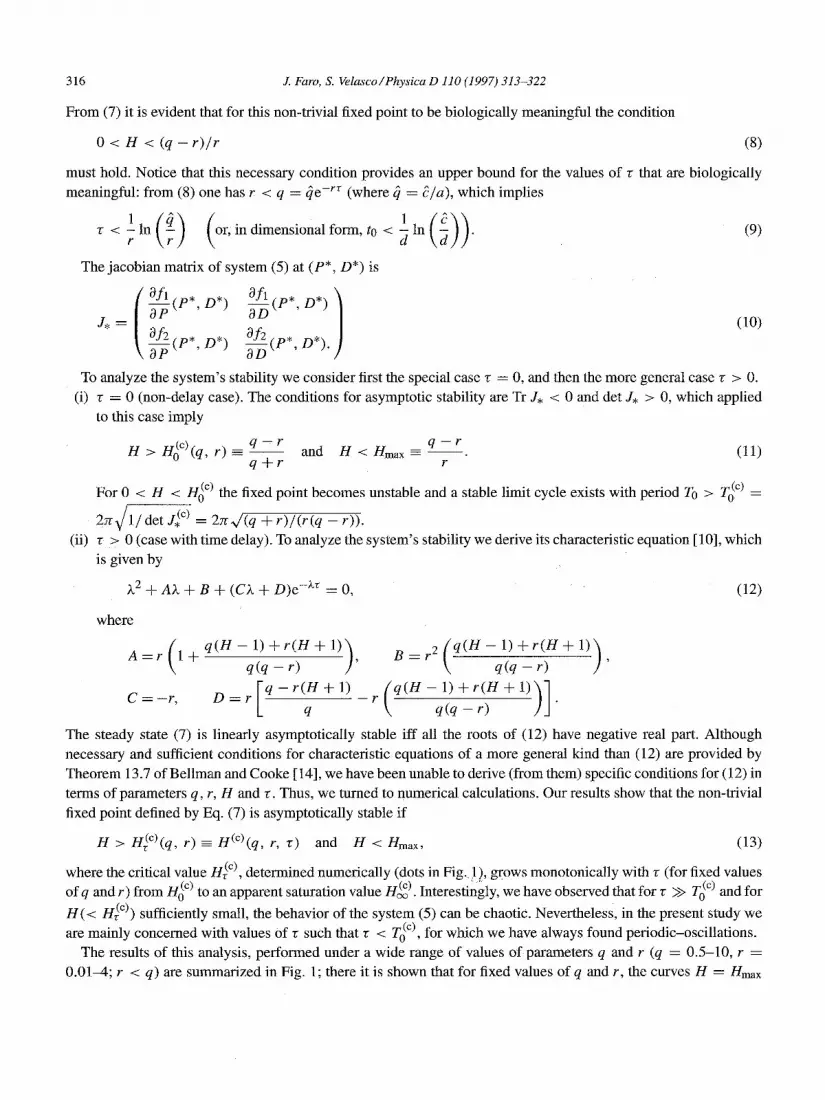
(e) where the critical value H~ , determined numerically (dots in F ig . l ! , gIows monotonically with v (for fixed values (c) (e) (c) o f q and r) from H(~ to an apparent saturation value H ~ . Interestingly, we have observed that for v >> T(j and for

H ( < H (c)) sufficiently small, the behavior of the system (5) can be chaotic. Nevertheless, in the present study we are mainly concerned with values of v such that r < T0 (c), for which we have always found periodic-oscillations.

The results of this analysis, performed under a wide range of values of parameters q and r (q = 0.5-10, r = 0.01-4; r < q) are summarized in Fig. 1; there it is shown that for fixed values of q and r, the curves H = //max


H

60

40

20

0

(i)

(II)

~ ° °

(III) . . . . i . . . . i . . . . i , , , , T . . . . i

10 20 30 40 50

H max

)

% Fig. 1. Stable and unstable regions in the parameter subspace (r, H) with q and r fixed. Curves H = Hrnax (solid line) and H = H (c) (dots) divide the parameter plane (r, H) in three regions. (I) H > Hmax: the steady state has no biological sense; (II) Hmax > H > Hr (c) : the steady state is asymptotically stable; and (III) 0 < H < Hr (c): the steady state is unstable and a stable limit cycle exists. The curve H = H~r c) (stripped line) was obtained with the simplified model and corresponds, in this model, to the critical values of H at which a stable steady state becomes unstable; this curve is therefore to be compared with the curve H = H (c) (dots). Other parameters: q = 10; r = 0.2.

(solid l ine) and H = H (c) (dots) divide the parameter p lane (r , H ) in three regions: (I) H > Hmax, for which the

steady state (7) has no biological sense; ( I I ) / /max > H > H (c), for which the fixed point (7) is asymptot ical ly

stable; and ( l i d 0 < H < H (c), for which the fixed point (7) is uns table and a stable l imit cycle exists.

4. A simplified model

If the delay r is small enough so that D does no t vary too rapidly over the t ime interval [t - z, t], one may

approximate D ( t - r ) with

D ( t - r ) "~ D ( t ) -- z D ( t ) . (14)

With this approximat ion, and after appropriate algebraic rearrangement , model (5) becomes

P ( t ) P ( t ) ( l P ( t ) ) (1 + r r ) P ( t ) D ( t ) = -- -- ~ f l ( P , D) , (15a) H + (1 + r q ) P ( t )

/ ) ( t ) = q(1 + r r ) P ( t ) D ( t ) _ r D ( t ) =-- f 2 ( P , D) . (15b) H -t- (1 -t- r q ) P ( t )

As for mode l (5), one easily checks that (7) is also the on ly non-t r ivia l fixed point of model (15). Again, to analyze

the stability of (15) the eigenvalues of its j acob ian matr ix have to be investigated. F rom (15) one gets

H(1 + rr)D* (!6) 0fl0p ( p . , D*) = 1 -- 2 P* - ( H + (1 + ~ : q ) p . ) 2 '


Ofl ( p , , (1 + r r ) P * (17) D * ) = H + ( I + r q ) P * '

o f 2 ( p , , Hq(1 + r r ) D * D*) = ( H + (1 + vq )P* ) 2 ' (18)

o f 2 (q -- r )P* -- H r (P*, D*) = = 0. (19)

H + (1 + vq)P*

Then, taking into account (7), the conditions for stability lead to

(q - r )(1 + vq) n > /~(C)(q, r ) =- and H < Hmax. (20)

q + r + 2rqv

We show also in Fig. 1 the dependence of Hr (c) on v for fixed values of q and r (dashed line). Notice that in

a similar fashion as Hr (c),/Tr (c) grows monotonical ly from H0 (c) to a saturation value; for model (15) this value is

given by H~) = (q - r ) /2r . Moreover, the results summarized in this figure also indicate that the relationship

_ hoids To determine the extent/~(c) deviates from H~ (c), we calculated/Tr (c) and H~ (c) for v ranging from 0 to r = 5 % To(c),

under the above range of parameter values. The results of these calculations, summarized in Fig. 2, indicate that for

r << To(c) there is an excellent agreement be tween/~r (c) and H~ (c).

6

-1- 5

4 u 3

<-~- -.. , 2 x

o 1 o " - 0

q = 0 . 5 r = 0.01 To(C) = 64.1

6

5

4

3

• 2

1

0 0.5 1 1.5 2 2.5 3

q = 0 . 5 r = 0 . 3 Told = 23.9

0.2 0.4 0.6 0.8 1

~ 6 -r"

5

-1- 4 I

~ , 3 <'1"

---- 2 × g 1

0

q = 1 0 r = 0 . 2 To(C) = 14.3

5

4

3

2

1

0

q = 10

r = 4 • Told = 4.8

o e e e o e

~oO o

0.1 0.2 0.3 0.4 0.5 0.6 0.7 0.05 0.1 0.15 0.2

17 17

Fig. 2. The percentage of deviation of H~r c) from Hr (c) is shown as a function of r. In each case the maximum value of r is 5% of the corresponding value of the limit cycle period at critical H and r = 0 (i.e. T0(C)). Note that at v = 2% TO(c) the differences between H~rr c)

and H (c) reduce to less than 3%.


5. I n f l u e n c e o f 7" o n p e r i o d s a n d a m p l i t u d e s

In the simplified model, for H : ~¢(c) the period is given by

~'(c) _ 2PT / q + r + 2qrr ~f~e~ j,(c) -- 2zr r(q -- r)

where j,(c) is the jacobian matrix of model (15) at (P*, D*) with H = ~(c). However, analytical expressions for

periods and amplitudes cannot be obtained in general, and so their values must be derived numerically. We have performed such a numerical study, for the above range of parameter values, to determine the effect

of a time delay T << T0 (c) on periods and amplitudes in both the original and the simplified models. The results,

summarized in Figs. 3 and 4, demonstrate that for T << T0 (c) the periods and amplitudes of oscillations obtained with the simplified model are very close to those obtained with the original model, which deviate rapidly and neatly

200

150

100

50

r 'a , l~ q = 0,,5

~,... ~3 ,1~ " r = 0.01

I I I

0!8 Ill0 112 A[ 1.41 Ill 1.6

[ q - 0 5

60 L ~ " " . . r = 0-3

40 - ~ ...... 2 " . .

Iii iJ 0 I I I

0 .10 0 .15 0 . 2 0 0 . 2 ~ "~

80 q = 10 14 - q = 10 ~ . ~ . ~ X I ~ ' , x r = 4 r = 0.2 12 ~...~.

60 10 "-. " " - . "

8 "~--. ,. • 6 " l :3"l~'n

I I I. I I I-I I I I I I I I A r-~ I 0.5 1.0 1.5 20 a'" 2.5 3.0 3.5 0 . 2 5 0 . 3 0 0 . 3 5 0 . 4 0 0 . 4 5 ~.50~0.55

p a r a m e t e r H p a r a m e t e r H

Fig. 3. Effect of low values of time delay z on periods. Time delays are: z = 0 (solid lines); r = 1% T0 (c) (triangles, time-delay model; dotted lines, simplified model); r = 2% TO(c) (squares, time-delay model; stripped lines, simplified model). In each case, parameter H was varied systematically below the corresponding critical value and the periods of the oscillations were calculated from time series (after discarding a transitory) by using a FFT.


0.7

0.6

0.5

~1 0.4

I~ 0.3

0.2

0.1

0.0

q = 0 . 5 ~ . . ~ r = 0.01

-%, b...

iN~ "" "';~ "~'. ">" "123,

0.8 1.0 1.2 1.4 1.6

1.0

0 .8

0.6

0.4

0.2

0.0

, ... ~.~ "'"'..~.. .... q = 0.5 ~ ~ . ~ . . . . . r = 0.3

0'20 1.0 q = 10 1.0

. . . ~ .. r = 0.2

"', ~ 0.8 0.8 ~:... . .

• ~ 0.6 "" 0.6 ~. ",, []-.,,

0.4 }~". " " ' , 0.4 ~I "~" '~

0.2 \ ".~ ",,,, 0.2

0.0 ~ 1 I I ,¢.. I I ,--~. 0.0 0.5 1.0 1.5 2.0 ~ 2.5 3.0 3.5

parameter H parameter H

q = 10 ~ - = 2 1 ~ - - . . r = 4 ~ ' ' ~ . ....... ...~-.......

I I I I \ I ,,'~l ,.-.-, ~' I 0.25 0.30 0.35 0.40 0.45 ~.50 '-"0.55

Fig. 4. Effect of low values of time delay r on amplitude s. Time delays and symbols are as in Fig. 3.

for increasing r from the values obtained in the model with r = 0. Moreover, whether the original or the simplified model, both period (Fig. 3) and amplitude (Fig. 4) increase for increasing r, this increase being larger when r decreases. Besides, our calculations indicate that for H < Hr (c) and for H < Hr (c), the corresponding periods T'r and Tr are bounded, respectively, by Tr (c) and Tr (c), i.e. T'r > ~'(c) and Tr _> Tr (c), and increase monotonically with

decreasing H (Fig. 3). Similarly, the amplitudes in both models increase with decreasing H (Fig. 4). Further, we have observed in all our simulations with r << T0 (c) that the transient regimes are nearly the same in both models

and that there is only a small phase shift of oscillations in the simplified model compared to those in the original model (not shown). These results demonstrate that for r << T0 (c) the simplified model retains much of the essential information of the original model.

6. E s t i m a t i o n o f e f fec t ive p a r a m e t e r s

When the simplified model (15) is expressed in dimensional form and in a way akin to that of model (4) with

to = 0 (i.e. model (1)) one gets


[~(t) = a P ( t ) (1 k ~ t ) ) bP(t)D(t)h + P (t) ' (21a)

[~(t) = g P ( t ) D ( t ) _ dD( t ) , (21b) + P( t )

where/), ~, h are given by

{) = /~e-dt°(1 + tod) ~ _-- ~e-dt°(1 + tod) ~ _ h (22) 1 + to~e -dtO ' 1 + to~e -dto ' 1 + to~e -dto

Thus, the only parameters affected by considering a time delay are the prey-predator interaction constants (/; and ~) and the half-saturation food uptake (h). Further, from (22) and recalling that d < c (r < q, see (8)) it is easy to see that the following inequalities hold:

1) < b = be -at° < l), ~ < c = ~e -dr° < ~, h < h. (23)

The good approximation obtained with the simplified model (21) and (22) suggests that in order that a non- time delay model like model (1) behaves in the same way as a similar model with time delay (e.g. model (2)), its "interaction" parameters as well as its "half-saturation food uptake" parameter must differ from the corresponding ones in the time-delay model and, so, must be considered as effective parameters (actually, this is the case when parameters are obtained phenomenologically from the fitting of a model behavior to empirical data [7]). The present approximation, however, allows to estimate those effective parameters in terms of the empirically obtained parameter values corresponding to individual processes. Further, it becomes clear that effective parameters are smaller than the real (empirical) ones. Moreover, this approximation provides a way to realize where and how is "acting" the effect due to a time delay. Finally, we note that a mechanistic interpretation of the effective parameters b, ~,/ t is not easily derived from (22). However, comparison of models (21) and (2) suggests a qualitative explanation of why time delay affects the rates (per unit of predator) of prey consumption and growth of predator: since terms {~P(t )D(t ) / (h + P( t ) ) and ?P(t)D(t) / ([~ + P( t ) ) in model (21) must have the same values as the corresponding terms in model (2), and since introducing a time delay implies that Da(t) < D(t) , it follows that the following inequalities must hold:

[~P(t) bP( t ) 8P( t ) ~P(t )

kt + P( t ) h + P ( t ) ' h + P( t ) h -I- P(t)"

(Notice that these inequalities can also be obtained, formally, from (22) and (23).) That is, considering a non- zero time delay implies that the mature predator subpopulation must be more effective, per individual, than the corresponding population when it is assumed an instantaneous maturation (i.e. without time delay).

7. Conclusions

Time delays have been recognized as a critical factor determining whether predation promotes prey stability or prey instability in many predation systems [7,8]. The study of dynamical models incorporating time delays is, however, hampered by the fact that time delays not only introduce difficult mathematical complications specific of each model family, but also make those models much less intuitive. We propose here that a way to overcome these difficulties in many instances is to substitute the variables x (t - T) by x (t) - r2 (t). To analyze this proposal in detail we focused on a particular but widely used two species prey-predator family of models. A comparative study of the original model (with time delay > 0) and the resulting simplified model was performed, both analytically and

322 3". Faro, S. Velasco/Physica D 110 (1997) 313-322

numerically by computer simulations for a wide range of values of the parameters involved. The results demonstrate

that for values of r sufficiently small compared with the period characteristic of the non-delay model (T0 (c)) the

periods and amplitudes of oscillations obtained with the simplified model are very close to those obtained with the

original model. The same is true with respect to the boundary (in parameter space) between the regions leading

either to a stable non-trivial fixed point or to a limit cycle. Moreover, the boundary in the simplified model can be

calculated analytically in an exact form. The proposed approach to study time-delay models provides, thus, a very

good approximation of those models, but without the difficulties introduced by time delays, and hence it is expected

to be a useful one. Finally, it is interesting to note that, when the effective parameters in the simplified model are

calculated and compared to the corresponding parameters in the model with T = 0, one can perceive immediately

where is "acting" the effect due to a time delay.

References

[1] J.D. Murray, Mathematical Biology (Springer, New York, 1990). [2] J.M. Cushing, A simple model of cannibalism, Math. Biosc. 78 (1991) 21-46. [3] C. Kohlmeier and W. Ebenh6h, The stabilizing role of cannibalism in a predator-prey system, Bull. Math. Biol. 57 (1995) 401-411. [4] T.H. Keitt and A.R. Johnson, Spatial heterogeneity and anomalous kinetics: Emergent patterns in diffusion-limited predatory-prey

interaction, J. Theoret. Biol. 172 (1995) 127-139. [5] W.G. Wilson, E. McCauley and A.M. De Boos, Effect of dimensionality on Lotka-Volterra predator-prey dynamics: Individual

based simulation results, Bull. Math. Biol. 57 (1995) 507-526. [6] A. Gragnani and S. Rinaldi, A universal bifurcation diagram for seasonally perturbed predator-prey models, Bull. Math. Biol. 57

(1995) 701-712. [7] E. Korpimaki and C.J. Krebs, Predation and population cycles of small mammals, A reassessment of the predation hypothesis,

BioScience 46 (1996) 754-764. [8] V. Volterra, Legons sur la th~orie math~matique de la lutte pour la vie (Gauthier-Villars, Paris, 1931). [9] J.M. Cushing, Integrodifferential equations and delay models in population dynamics, Lecture Notes in Biomath. 20 (1977) 1-196.

[ 10] K. Gopalsamy, Stability and Oscillations in Delay Differential Equations of Population Dynamics (Kluwer Academic Publishers, Netherlands, 1992).

[11] Y. Kuang, Delay Differential Equations with Applications in Population Dynamics (Academic Press, Cambridge, MA, 1993). [12] W.B. Case, Time-delay oscillator and instability: A demonstration, Am. J. Phys. 62 (1994) 227-230. [13] A.J. Lotka, Elements of Physical Biology (Williams and Wilkins, Baltimore, 1925). [14] R. Bellman and K.L. Cooke, Differential-Difference Equations (Academic Press, New York, 1963).

Documents

An approximation for prey-predator models with time delay