An Axiomatic Framework for Influence DiagramComputation with Partially Ordered Utilities

Nic WilsonCork Constraint Computation Centre

University College Cork, Irelandn.wilson@4c.ucc.ie

Radu MarinescuIBM ResearchDublin, Ireland

radu.marinescu@ie.ibm.com

AbstractThis paper presents an axiomatic framework for influence di-agram computation, which allows reasoning with partially or-dered values of utility. We show how an algorithm based onsequential variable elimination can be used to compute the setof maximal values of expected utility (up to an equivalencerelation). Formalisms subsumed by the framework includedecision making under uncertainty based on multi-objectiveutility, or on interval-valued utilities, as well as a more quali-tative decision theory based on order-of-magnitude probabil-ities and utilities.

1 IntroductionActions can lead to many different kinds of consequences,for example, financial gain/loss, risk to health, effect onthe environment or gain/loss to reputation. It may not bepossible to map the various potential consequences of aset of actions to the same scale of utility in a way thatavoids making essentially arbitrary choices. It is thus nat-ural to consider notions of imprecise utility and multi-attribute/objective utility, where utility values are only par-tially ordered.

We consider decision making under uncertainty using in-fluence diagrams, but where we allow more general notionsof uncertainty than probability, and more general notions ofutility functions, which, in particular, allow utility values tobe only partially ordered. We construct an axiomatic frame-work, listing properties of a formalism that allow maximal(generalised) expected utility to be computed by sequentialelimination of all the variables.

In general terms, variable elimination algorithms can beviewed as follows. We have a collection Θ of functions,where each function in Θ only involves a small number ofvariables. In the case of influence diagram computation, Θcontains both probability functions and utility functions. Θis used as a compact representation (or decomposition) ofa function

⊗Θ on all the variables, equalling a combina-

tion of all the functions in Θ. For example, in a Bayesiannetwork, Θ consists of a collection of conditional probabil-ity functions and

⊗Θ is the joint probability distribution.

Since⊗

Θ involves all the variables, it will be a huge ob-ject to represent explicitly.

Copyright c© 2012, Association for the Advancement of ArtificialIntelligence (www.aaai.org). All rights reserved.

For a standard influence diagram we have both chance anddecision variables, and we eliminate chance variables with asum operator, and decision variables with a max operator.We can compute the maximum expected utility by applyinga sequence of sum and max eliminations to

⊗Θ, eliminat-

ing all the variables. Performing combinations leads to func-tions involving larger sets of variables, which is expensivein terms of both computational cost and time. One thereforewould like to delay performing computations where possi-ble. Thus, when eliminating a variable X , with, for exam-ple, the

∑operator, one transforms Θ to a collection Θ′,

which includes only functions that don’t involve X , and issuch that

∑X(⊗

Θ) =⊗

Θ′. Crucially, the functions inΘ that don’t involve X are left unchanged, so still appear inΘ′.

We first define (Section 2) our axioms for uncertainty andutility functions, which are the properties that we will use forthe variable elimination algorithms. We describe some for-malisms that satisfy the axioms, including interval-valuedutility, multi-objective utility and order of magnitude prob-ability and utility (Section 3). Section 4 shows how bothchance variables and decision variables are eliminated. Toeliminate a variable involves replacing the current collec-tion of generalised probability and utility functions with anew set whose combination is equivalent to the marginal ofthe initial set. Section 5 defines influence diagram systems,which involve the form of uncertainty and utility functionsthat are generated by an influence diagram. Section 6 showsthat one can iteratively eliminate all the variables to obtainthe maximum value of expected utility for the case whereutility values are totally ordered.

We go on to consider the case where values of utility areonly partially ordered (Section 7); then there will often notbe a unique maximal value of (expected) utility, but a set ofthem. To compute this set we need to perform operations onsets of utility values. In Section 8 we give the main resultof the paper, which shows how to compute, by sequentialvariable elimination, a set of utility values that is equivalent,in a particular sense, to the set of maximal values of ex-pected utility. Section 9 discusses related work, and Section10 concludes. The Appendix includes some of the proofs,with more complete proofs being in a supplementary docu-ment (Wilson and Marinescu 2012).

210

Proceedings of the Thirteenth International Conference on Principles of Knowledge Representation and Reasoning

2 Uncertainty And Utility FunctionsIn standard influence diagrams, probability potentials takenon-negative real values, and utility functions take real val-ues. In Section 2.1 we give properties of generalised proba-bility and utility values which will still allow correct variableelimination algorithms.

Most of the properties of positive reals are still assumedfor generalised probability values, the most important ex-ception being that we do not assume a cancellation propertyfor addition. The properties assumed for generalised utilityvalues are much weaker than those satisfied by the real num-bers; in particular, we allow partially ordered utility values,which will be useful for expressing imprecise informationabout utilities, or multi-objective utilities.

Section 2.2 defines the generalised probability and utilityfunctions, along with combination and marginalisation op-erators, generalising definitions for standard probability andutility.

2.1 Uncertainty-Utility Values StructuresAn uncertainty values structure is defined to be a tuple〈Q,+,×, 0, 1〉 that is a positive commutative semiring withmultiplicative inverses. In other words: + and × are bothcommutative and associative binary operations on set Q,with additive identity element 0 (so q+0 = q for all q ∈ Q),multiplicative identity element 1 (so q×1 = q for all q ∈ Q)which also satisfies q × 0 = 0 for all q ∈ Q, and, for allp, q ∈ Q, p + q = 0 if and only if p = q = 0; also, ×distributes over +, i.e., (p+ q)× r = (p× r) + (q× r). Fur-thermore, it is assumed that multiplicative inverses exist forall non-zero elements of Q, so that for all q ∈ Q−0 thereexists some (unique) element q−1 ∈ Q with q × q−1 = 1.

A utility values structure is defined to be a tuple 〈U,+, 0〉such that + is a commutative and associative binary opera-tion U with identity element 0.

A weak uncertainty-utility values structure (abbrevi-ated to weak u.u.v. structure) is defined to be a tu-ple U = 〈Q,+Q,×Q, 0Q, 1, U,+U , 0U ,×QU 〉, where〈Q,+Q,×Q, 0Q, 1〉 is an uncertainty values structure,〈U,+U , 0U 〉 is a utility values structure, and ×QU is a func-tion from Q × U → U satisfying the properties (∗1), (∗2)and (∗3) below, for arbitrary u, u1, u2 ∈ U and q, q1, q2 ∈ Q(dropping the (·)Q and (·)U subscripts since there is no am-biguity):

(∗1) 1× u = u and 0× u = 0U ;(∗2) q1 × (q2 × u) = (q1 × q2)× u;(∗3) q × (u1 + u2) = (q × u1) + (q × u2).

We further define U to be an uncertainty-utility values struc-ture (u.u.v. structure) if it is a weak uncertainty-utility valuesstructure and satisfies also:

(∗4) (q1 + q2)× u = (q1 × u) + (q2 × u).Q will contain the probability-like values, and U will con-tain the utility-like values.

Disjunctive Operations: When we are eliminating deci-sion variables in an influence diagram computation, we usea max operator. We generalise this to a disjunctive opera-tion, as defined below. For the totally ordered case (see the

end of Section 6), we use max as the disjunctive operator;for the partially ordered case in Section 7, we use max oversubsets of utility values.

Let U = 〈Q,+Q,×Q, 0Q, 1, U,+U , 0U ,×QU 〉 be a weaku.u.v. structure. Let ∨ be a binary operation on U . We saythat ∨ is a disjunctive operation for U if ∨ is a commutativeand associative operation on U such that both +U and ×QUdistribute over ∨, so that for any q ∈ Q and all u1, u2, u3 ∈U , u1+(u2∨u3) = (u1+u2)∨(u1+u3), and q×(u1∨u2) =(q × u1) ∨ (q × u2).

Operation respecting ordering: Let T be some set andlet be some function from T × U to U . We say that respects binary relation on U if for all t ∈ T and all ele-ments u1, u2 of U , u1 u2 ⇒ t u1 t u2. (This canbe also be viewed as being monotonic with respect to .)

We say that U respects if both +U and ×QU respect .Suppose that U respects total order . If we define ∨

to be maximum with respect to , then ∨ is a disjunctiveoperation.

2.2 Combining And Marginalising UncertaintyAnd Utility

We consider a set of variables that is partitioned into X andD, where the elements of X are known as chance variables,and the elements of D are known as decision variables.Each element Y ∈ X ∪ D has an associated set of possi-ble values ΩY . We also write, for S ⊆ X ∪D, ΩS for theCartesian product of ΩY over Y ∈ S.

Let U = 〈Q,+Q,×Q, 0Q, 1, U,+U , 0U ,×QU 〉 be a weaku.u.v. structure. A U-uncertainty function over X ∪D is afunction P from ΩS to Q, for some S ⊆ X ∪D, known asthe scope of P, and denoted by sc(P).

A U-utility function over variables X ∪D is a functionU from ΩS to U , for some S ⊆ X∪D, where S is the scopesc(U) of U.

We say that P involves Y if sc(P) 3 Y . If T ⊇ S =sc(P) and x ∈ ΩT then we also write P(x) as an abbrevi-ation for P(x↓S), where x↓S is the projection of x to vari-ables S. Similarly, for U-utility function U.

Let Φ be a collection (i.e., a multiset) of U-uncertaintyfunctions over X ∪ D. We define their combination∏

Φ =∏

P∈Φ P to be the U-uncertainty function withscope S =

⋃P∈Φ sc(P), given by, for x ∈ ΩS , (

∏Φ)(x) =∏

P∈Φ(P(x)), where the last use of∏

refers to repeatedapplication of the (associative and commutative) operation×Q.

Analogously, we define, for collection Ψ of U-utility func-tions over X ∪ D, their combination

∑Ψ =

∑U∈Ψ U

to have scope S =⋃

U∈Ψ sc(U), and to be given by(∑

Ψ)(x) =∑

U∈Ψ U(x), where the last∑

refers to it-erative use of +U .

If P is a U-uncertainty function and U is a U-utility func-tion then P × U is a U-utility function with scope S =sc(P) ∪ sc(U) given by (P ×U)(x) = P(x) ×QU U(x),for any x ∈ ΩS . (Thus U-utility functions can representexpected utility as well as input utility functions.)

211

Generating a marginalisation operator from an opera-tion on utility values: Suppose that is some commuta-tive and associative operation on U . Let U be a U-utilityfunction and let Y ∈ X ∪ D be a variable in the scope ofU. We define

⊙Y U to be the U-utility function with scope

S = sc(U)−Y given by (⊙

Y U)(x) =⊙

y∈ΩYU(xy),

for x ∈ ΩS , where xy is assignment x extended with Y = y.This defines operation

∑Y , based on operation = +, and∨

Y , based on disjunctive operation ∨.

3 Example FormalismsWe give some examples of formalisms that satisfy the ax-ioms defined above. The results given later in this paperimply that, for any of these formalisms, the maximal valuesof expected utility can be computed (up to equivalence) by avariable elimination algorithm.

3.1 Upper And Lower UtilityIt can sometimes be hard to determine precisely a utilityvalue. To allow a representation of imprecise utility, we canlet utility functions assign pairs of utility values instead ofsingle values, representing a lower and an upper value ofutility. For an influence diagram computation (see Section5), each policy π, dynamically assigning the decision vari-ables, has an associated lower expected utility LEU(π) andan upper expected utility UEU(π).

A natural ordering on these (expected) utility pairs is thepointwise one given by 〈u, v〉 〈u′, v′〉 if and only ifu ≥ u′ and v ≥ v′. That is, π is at least as good as π′ ifLEU(π) ≥ LEU(π′) and UEU(π) ≥ UEU(π′). We thendefine U to consist of the set of all pairs 〈u, v〉 of real num-bers with u ≤ v. The sum of two pairs 〈u1, v1〉 and 〈u2, v2〉is performed pointwise, i.e., to be 〈u1 + u2, v1 + v2〉. Theadditive identity utility element is the pair 〈0, 0〉. For proba-bility value p and utility pair 〈u, v〉, p × 〈u, v〉 is defined tobe 〈p × u, p × v〉. This gives rise to an u.u.v. structure〈R+,+,×, 0, 1, U,+U , 〈0, 0〉,×QU 〉 that respects the par-tial order . Since utility values are only partially ordered,we may well have more than one maximal value of expectedutility; we are interested in being able to compute the set ofmaximal (i.e., undominated) values of

⟨LEU(π),UEU(π)

⟩over all policies π.

Multi-Objective Utility A related system (which is math-ematically a generalisation) is based on multi-objective util-ity. One may have more than one independent scale of util-ity, for example, one based on monetary gain, and one basedon risk to health. Again, scalar multiplication and additionare performed pointwise, and we can use the same idea forthe ordering. Alternatively, since the product (Pareto) order-ing is a rather weak one, instead one may want to considerimprecise trade-offs between the scales of utility. The order-ing can be strengthened to take such trade-offs into account,whilst still maintaining the monotonicity properties.

A further related system is multi-agent probability andutilities. Each of a number m of agents makes a judgementof the probability and utility values, which are each repre-sented as vectors of m real values.

3.2 Order Of Magnitude CalculusWe consider the order of magnitude probability and utilitysystem from (Wilson 1995), which can be viewed as a deci-sion theory for kappa (ranking) functions (Goldszmidt andPearl 1996). (A very different linear utility theory for kappafunctions is given in (Giang and Shenoy 2000).) Let O =〈σ, n〉 : n ∈ Z, σ ∈ +,−,± ∪ 〈0,∞〉, where Z isthe set of integers. The element 〈±,∞〉 will sometimes bewritten as 0, and element 〈+, 0〉 as 1. We also define O± =〈±, n〉 : n ∈ Z ∪ ∞, and O+ = 〈+, n〉 : n ∈ Z.

Elements ofO are interpreted in terms of polynomials (orrational functions) in a parameter ε. ε can be consideredas an infinitesimal, or, alternatively, a very small unknownnumber. 〈+, n〉 represents a function which is positive andof order εn, and 〈−, n〉 is negative and of order εn. Whenwe add a positive and a negative value, both of order εn, theanswer can be positive or negative, and of order εm for anym ≥ n. We write this imprecise value as 〈±, n〉.

Multiplication: For 〈σ,m〉, 〈σ′, n〉 ∈ O, let 〈σ,m〉 ×〈σ′, n〉 = 〈σ ⊗ σ′,m+ n〉, where∞+m = m+∞ =∞for m ∈ Z ∪ ∞, and ⊗ is the natural multiplication ofsigns: it is the commutative operation on +,−,± suchthat + ⊗ − = −, + ⊗ + = − ⊗ − = +, and for anyσ ∈ +,−,±, σ ⊗± = ±.

Addition: Commutative operation + is given by 〈σ,m〉+〈σ′, n〉 = 〈σ,m〉 ifm < n, and equals 〈σ⊕σ′,m〉 ifm = n,where +⊕+ = +,−⊕− = −, and otherwise, σ⊕σ′ = ±.

Ordering: We use a slightly stronger ordering than thatdefined in (Wilson 1995). Transitive relation on O isgiven by: 〈+, l〉 〈σ,m〉 〈−, n〉, for any l,m, n suchthat l, n ≤ m, and any σ ∈ +,−,±.

We will define an u.u.v. structure U for the order of mag-nitude case. We define U to be O and Q to be O+ ∪ 0.The previously stated properties including (∗1), (∗2), (∗3),and (∗4) all hold, and the operations respect the ordering.

Proposition 1. Define UO to be the tuple 〈O+ ∪0,+,×, 0, 1,O,+, 0,×〉. Then UO is an uncertainty-utility values structure that respects partial order , i.e., is respected by + and the operation× : O+∪0×O → O.

4 Elimination Of VariablesIn this section we will consider an u.u.v. structure U, and apair (Φ,Ψ), where Φ (respectively, Ψ) is a collection of U-uncertainty (respectively, U-utility) functions over X ∪ D.We assume that each variable in X ∪D is involved in someelement of Φ ∪Ψ.

A pair (Φ,Ψ) will be considered as a compact represen-tation of the (overall) utility function

∏P∈Φ P×

∑U∈Ψ U.

We write⊗

(Φ,Ψ) =∏

P∈Φ P×∑

U∈Ψ U.We will be interested in computing a generalised expected

utility corresponding to the result of eliminating all variablesfrom

⊗(Φ,Ψ). In Sections 4.1 and 4.2 we will show how

to eliminate chance variables and decision variables.

212

In eliminating a chance variableX we generate a new pair(Φ′,Ψ′) that doesn’t involve X such that

∑X

⊗(Φ,Ψ) =⊗

(Φ′,Ψ′). This involves combining functions that involveX; importantly, functions that don’t involve X are left asthey are. Similar remarks apply for the elimination of a de-cision variable.

4.1 Elimination Of A Chance VariableLet Φ63X be the multiset containing the elements of Φ notinvolving variable X , i.e., with sc(P) 63 X , and let Φ3Xbe the other elements in Φ. Let P+ =

∏P∈Φ3X

P be thecombination of elements of Φ involving variable X , and letPXΦ be

∑X P+. Let Φ′ = Φ63X ∪ PXΦ .

Similarly, let Ψ63X be the multiset containing the elementsof Ψ not involving X , and let Ψ3X be the other elements inΨ. For U ∈ Ψ3X , define U−X to be 1

PXΦ×∑X(P+ ×U)

(where, in this equation, we define 10 to be 0). Let Ψ′ =

Ψ63X ∪ U−X : U ∈ Ψ3X.We define

∑X(Φ,Ψ) to be (Φ′,Ψ′). Note that no ele-

ment of Φ′ or of Ψ′ involves X . Also, in contrast with e.g.,(Jensen, Jensen, and Dittmer 1994), we don’t combine to-gether the utility functions involving X when eliminating achance variable X , since it’s not necessary.

Theorem 1. Let U be an uncertainty-utility values struc-ture, with associated summation operation

∑, let Φ be a

collection of U-uncertainty functions over X ∪D, let Ψ bea collection of U-utility functions over X ∪D. Then for anyX ∈ X which is involved in some element of Φ,∑

X

⊗(Φ,Ψ) =

⊗(∑X

(Φ,Ψ)).

In other words, using the definitions of Φ′ and Ψ′ givenabove,∑

X

(∏P∈Φ

P×∑U∈Ψ

U)

=∏

P∈Φ′

P×∑U∈Ψ′

U.

4.2 Elimination Of A Decision VariableWe say that P does not depend on variable Y if for ally, y′ ∈ ΩY and x ∈ ΩS where S = sc(P) − Y ,P(xy) = P(xy′). If so, we define P−Y to have scope Sand be given by P−Y (x) = P(xy) (for any y ∈ ΩY ).

Theorem 2. Let ∨ be a disjunctive operation for weakuncertainty-utility values structure U. Let D be a deci-sion variable in D, let Φ be a collection of U-uncertaintyfunctions over X ∪ D, none of which depend on variableD, and let Ψ be a collection of U-utility functions overX ∪ D. Define

∨D(Φ,Ψ) = (Φ−D,Ψ′′), where Φ−D =

P−D : P ∈ Φ, and Ψ′′ = Ψ63D ∪ ∨D

∑U∈Ψ3D

U.Then, ∨

D

⊗(Φ,Ψ) =

⊗(∨D

(Φ,Ψ)),

i.e., ∨D

(∏P∈Φ

P×∑U∈Ψ

U)

=∏

P∈Φ−D

P×∑

U∈Ψ′′

U,

5 Influence Diagram SystemsTheorems 1 and 2 show how to eliminate chance variablesand decision variables, respectively, using marginalisationoperators

∑X and

∨D on a pair (Φ,Ψ). We would like

to iteratively apply these to eliminate all variables, leadingto the maximum expected utility. However, Theorem 2 re-quires that, before eliminating decision variable D, the cur-rent set of uncertainty functions does not depend on D. Toensure that this condition holds for the iterative computation,we require restrictions on the elimination ordering, as wellas additional structure on the input collection of uncertaintyfunctions Φ.

Let U be a weak u.u.v. structure, and let P be an U-uncertainty function with scope S ⊆ X ∪ D. We say thatP is a constant function if it does not depend on any vari-able, i.e., there exists some value q ∈ Q such that for allx ∈ Ωsc(P), P(x) = q. We say that P is a conditional U-uncertainty function on X if X ∈ sc(P) and

∑X P is a

constant function.An Influence Diagram system (ID-system) over U is a pair〈G, (Φ,Ψ)〉, such that:

• G is a directed acyclic graph on X ∪D.

• Φ = PX : X ∈ X, where PX is a condi-tional U-uncertainty function on X with scope X ∪paG(X); (paG(X) means the set of parents of X , i.e.,Y : (Y,X) ∈ G);

• each element of Ψ is a U-utility function (whose scope isa subset of X ∪D).

• G restricted to D is a total order, which we write asD1, . . . , Dm.

• If (X,Di) ∈ G then (X,Dj) ∈ G for any j > i (this isthe no forgetting condition).

Collection Φ is a Bayesian network-style decompositionof a global uncertainty distribution, namely

∏Φ. Also,

∑Ψ

represents the overall utility function. Hence the function⊗(Φ,Ψ) represents the (generalised) probability times util-

ity function.(Y,Di) ∈ G means that the value of Y is known when

choosing the value of decision variable Di. Let Si bepaG(Di) for i = 1, . . . ,m. The choice of value of Di cantherefore depend on the values of variables in Si but no oth-ers.

A policy for this ID-system is a sequence (π1, . . . , πm)where πi is a function from ΩSi to ΩDi ; this represents whatvalue of Di is chosen given the available information: thealready observed chance variables, and previous choices ofdecision variables.

A policy π determines a value for each decision variableDi (which depends on the parents set Si). Given a utilityfunction U involving all the chance variables X, a policy πdetermines a utility function [U]π that involves no decisionvariables, by assigning their values using π. The expectedutility given policy π is given by EUπ =

∑X[⊗

(Φ,Ψ)]π .If the utility values set U is totally ordered with relation then maximum expected utility is maxπ EUπ , where max istaken with respect to .

213

Oil contents

Seismic results

Test?

Drill?

Drill payoff

Test payoff

Oil contents P(O)

dry wet soak

0 5 0.3 0.2

Test payoff U1(T)

Test?

yes -10

no 0

Drill payoff U2(O,D)

Oil cnt. Drill?

dry yes -70

dry no 0

wet yes 50

wet no 0

soak yes 200

soak no 0

Seismic results P(S | O,T)

Oil cnt. Test? closed open diffuse notest

dry yes 0.1 0.3 0 6 0

dry no 0 0 0 1

wet yes 0.3 0.4 0 3 0

wet no 0 0 0 1

soak yes 0.5 0.4 0.1 0

soak no 0 0 0 1

Figure 1: The oil wildcatter influence diagram.

For k = 0, . . . ,m − 1, let Ik be the set of chance nodeparents of Dk+1 that are not parents of any Di, for i ≤ k.Hence Ik is the set of chance nodes that Dk+1 depends on,but no earlier Di depends on. We also let Im be the otherchance nodes, that are not parents of any decision node.

A legal elimination sequence for an ID-system is a per-mutation Y1, . . . , Yn of the variables in X ∪D that extendsthe relation < given by: I0 < D1 < I1 < · · · < Dm < Im,so that, for i = 0, . . . ,m, each element X of Ii comes afterDi (if i ≥ 1) and before Di+1 (if i < m). For example,if Yj ∈ D1 and Yk ∈ I1 then we must have j < k. (Notethat the sequence is not necessarily compatible with G, sowe could have i < j and (Yj , Yi) ∈ G, when Yi and Yj areboth chance variables.)

Let τ be a sequence Y1, . . . , Yn of different elements inX ∪ D, and let ∨ be a disjunctive operation for U. Wedefine M+,∨

τ (U) to mean the result of iterative applicationof the marginalisations corresponding to sequence τ , i.e.,MY1

(MY2(· · · (MYnU) · · · ) where MY is

∑Y if Y is a

chance variable, and MY is∨Y if Y is a decision variable.

Note that the marginalisation operations are applied fromright to left, so that the Yn-marginalisation is performed first.

Suppose that U respects total order on U . As mentionedin Section 2.1, if we define ∨ to be maximum with respect to, then ∨ is a disjunctive operation. Then, for legal elimina-tion sequence τ , M+,∨

τ

(⊗(Φ,Ψ)

)can be shown (e.g., using

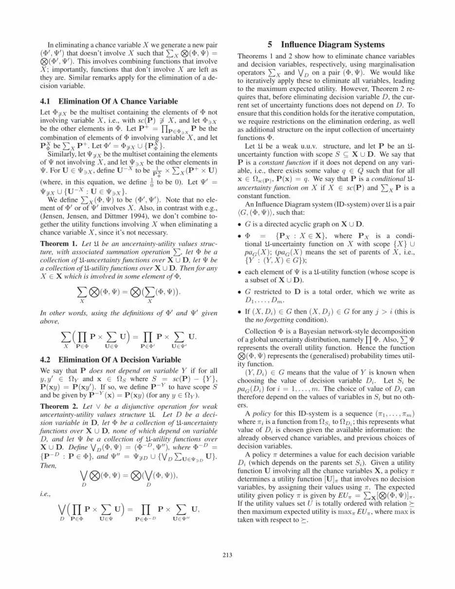
Proposition 5 below) to be the maximum value of expectedutility over all possible policies, i.e., maxπ EUπ .Example 1. Figure 1 shows the influence diagram of theoil wildcatter problem (adapted from (Raiffa 1968)). An oilwildcatter must decide either to drill or not to drill for oilat a specific site. Before drilling, they could perform a seis-mic test that will help determine the geological structure ofthe site. The test results can show a closed reflection pattern(indication of significant oil), an open pattern (indication ofsome oil), or a diffuse pattern (almost no hope of oil). Thespecial value notest indicates that the test results will not beavailable if the seismic test is not done. There are there-fore two decision variables, T (Test) and D (Drill), and two

chance variables S (Seismic results) and O (Oil contents).The probabilistic knowledge consists of the conditional

probability distributions P (O) and P (S|O, T ), while theutility function is the sum of U1(T ) and U2(D,O); thus weset Φ = P (O), P (S|O, T ) and Ψ = U1(T ), U2(D,O).There is a unique legal elimination sequence: τ =T, S,D,O (so that O is eliminated first). The maximum ex-pected utility, which equals M+,∨

τ

(⊗(Φ,Ψ)

), is thus equal

to∨T

∑S

∨D

∑O

(⊗(Φ,Ψ)

), where ∨ here means max.

The optimal policy is to perform the seismic test and to drillonly if the test results show an open or a closed pattern. Theexpected utility of this policy is 22.5.

πT = yes ; πD =

yes if S = openyes if S = closedno if S = diffuse

6 Elimination Of All VariablesWe show (Theorem 3 below) how all variables can be itera-tively eliminated for an ID-system. The proof uses iterativeapplication of Theorems 1 and 2, where the main difficultyis in showing that, when eliminating a decision variable D,none of the uncertainty functions P depend on D (see theconditions of Theorem 2). The conditions assumed on Φ inan ID-system imply this.

Theorem 3. Let U be an uncertainty-utility values structurewith operation + on utility values, and let ∨ be a disjunctiveoperation for U. Let I = 〈G, (Φ,Ψ)〉 be an ID-system overU, and let τ be a legal elimination sequence for I. Then

M+,∨τ

(⊗(Φ,Ψ)

)=⊗(

M+,∨τ

(Φ,Ψ

)).

The right-hand-side⊗(

M+,∨τ

(Φ,Ψ

))involves iterative

local computations, based on sequential elimination of vari-ables. When eliminating (marginalising out) a variable Ywe only deal with functions involving Y : the ones not in-volving Y are just left as they are. (The operator

⊗on the

right-hand-side will be easy and often be redundant, sincewe’ll typically just have a single utility value, representingexpected utility, when we’ve eliminated all the variables.)

Application for Totally Ordered Case: Suppose that is a total order on U such that +U and ×QU both respect, and again define ∨ to be maximum with respect to ,which is a disjunctive operation. As observed above in Sec-tion 5, the left-hand-side M+,∨

τ

(⊗(Φ,Ψ)

)in Theorem 3 is

equal to maximum value of expected utility over all possi-ble policies, i.e., maxπ EUπ . Hence Theorem 3 implies thecorrectness of an iterative variable elimination algorithm tocompute maximum expected utility. This applies to standardprobability and utility functions, and also to the simplifiedorder of magnitude systems defined in Section 8.5 of (Wil-son and Marinescu 2012).

The complexity is exponential in the largest scope of afunction generated by the algorithm, which is no more thanthe induced width of G′ (ordered according to the elimina-tion sequence), where G′ is G with an additional clique Sfor each input utility function with scope S.

214

7 Sets Of Utility Values For PartiallyOrdered Case

Let U be an uncertainty-utility values structure and let I =〈G, (Φ,Ψ)〉 be an ID-system over U. Suppose that the setof utility values U is only partially ordered, by relation. For finite set A of utility values we can consider theset of maximal ones max(A) consisting of all u ∈ Asuch that there does not exist a different element v ∈ Awith v u. We are interested in policies that generate amaximal value of expected utility, i.e., values of utility inmax EUπ : policies π. Towards this aim, we consideroperations on sets of utility values (in an analogous way tothe approach taken in Section 4.3 of (Fargier, Rollon, andWilson 2010) for the much simpler case where there are justutility functions, and in Section 3 of (Perny, Spanjaard, andWeng 2005)).

7.1 Operations On Sets Of Utility ValuesConsider an uncertainty-utility values structure U =〈Q,+Q,×Q, 0Q, 1, U,+U , 0U ,×〉. We extend addition andscalar multiplication of utilities to 2U , the set of subsets ofU , in the obvious way. For any A,B ⊆ U and q ∈ Q,define:

A+B = a+ b : a ∈ A, b ∈ B;q ×A = q × u : u ∈ A.

Given the uncertainty-utility values structure U =〈Q,+Q,×Q, 0Q, 1, U,+U , 0U ,×QU 〉, we define U∗ to bethe tuple U∗ = 〈Q,+Q,×Q, 0Q, 1, 2U ,+, 0U,×〉 (usingthe operations on sets as just defined). We have the follow-ing result:

Proposition 2. For any u.u.v. structure U, the associatedtuple U∗ is a weak uncertainty-utility values structure.

Unfortunately, property (∗4) (see Section 2.1) doesnot hold in general for sets, so U∗ is not neces-sarily an uncertainty-utility values structure. (q1 +q2) × A is equal, using the property (∗4) for U, to(q1 × a) + (q2 × a) : a ∈ A. On the other hand, (q1 ×A)+(q2×A) equals (q1 × a1) + (q2 × a2) : a1, a2 ∈ A.This implies that (q1 + q2) × A is a subset of (q1 ×A) + (q2 × A). However, they will very often not beequal. To give a simple example with bi-objective util-ity, let q1 = q2 = 0.5, and let A = (1, 0), (0, 1),using the pointwise operations on pairs of real numbers.(q1 + q2) × A = 1 × (1, 0), (0, 1) = (1, 0), (0, 1),whereas (q1 × A) + (q2 × A) = (0.5, 0), (0, 0.5) +(0.5, 0), (0, 0.5) = (1, 0), (0.5, 0.5), (0, 1).

However, in Section 7.3 we will define an equivalencerelation that ensures that property (∗4) holds up to equiva-lence.

7.2 Ordering On Sets Of UtilitiesWe assume a partial ordering that is respected by U, i.e.,is a partial order on U and operations +U and ×QU respect. If a b then we say that a dominates b. We write forthe strict part of , so that a b if and only if a b anda 6= b.

ForA ⊆ U , define max(A), the maximal elements ofA,to consist of all a ∈ A such that there does not exist b ∈ Awith b a. Hence, max(A) is the set of undominatedelements of A.

For A,B ⊆ U we say that A < B if every element ofB is dominated by some element of A (so that A containsas least as large elements as B), i.e., if for all b ∈ B thereexists a ∈ A with a b. Relation < on 2U is a reflexiveand transitive relation. We define equivalence relation ≈ byA ≈ B if and only if A < B and B < A.

7.3 The Equivalence Relation ≡ Between UtilitySets

The convex closure C(A) of a (finite or infinite) subset Aof U is defined to consist of every element of the form∑ki=1(qi×ai), where k is an arbitrary natural number, each

ai is in A, each qi is in Q, where∑ki=1 qi = 1.

We will argue that certain different sets of (expected) util-ity values can reasonably be considered as equivalent. Firstof all, if A contains elements u and v with u v, thenwe can consider that A and A − v are equivalent. Thesecond consideration is based on convex closure. For clar-ity, let’s consider the case where the uncertainty values areprobability values (but that the utility values may be partiallyordered, such as for multi-objective utility or interval-valuedutilities). If an agent can generate an expected utility valueu with policy π, and utility value u′ with policy π′ then theymay choose an independent auxiliary event E (e.g. basedon a random number generator such as rolling a die) withchance p, and choose π if E holds and π′ otherwise. (Fromthe outside it may not even be possible to tell that they aredoing this, since we only see the choices they make.) Theexpected utility is then pu + (1 − p)u′. More generally, ifone can achieve any of a setA of expected utility values, onecan generate any element of C(A) by using the same kind ofprocedure. Thus, A and C(A) are equivalent in a naturalsense.

We define equivalence relation ≡ on subsets of U by:

A ≡ B if and only if C(A) ≈ C(B).

Two sets of utility values are therefore considered equivalentif, for every convex combination of elements of one, there isa convex combination of elements of the other which is atleast as good (with respect to the partial order on U ). Wehave A ≡ C(A), and, if A is finite then A ≡ max(A).Moreover, if A ≡ B then max(C(A)) = max(C(B))(and the converse often holds). The equivalence relationis respected by scalar multiplication, addition and union ofsubsets of utility values:

Proposition 3. Let A, B and C be subsets of U , and let qbe an element of Q. Suppose that A ≡ B. Then (i) q ×A ≡q ×B; (ii) A+ C ≡ B + C; (iii) A ∪ C ≡ B ∪ C.

As observed above, Property (∗4) does not necessarilyhold for sets of utility values. However, it does hold forconvex sets, and a corresponding property based on ≡ holdsgenerally:

215

Proposition 4. Consider u.u.v. structure U, written as〈Q,+Q,×Q, 0Q, 1, U,+U , 0U ,×〉, which respects the par-tial order . Then the associated weak u.u.v. structureU∗ satisfies the following variant of Property (∗4): for allq1, q2 ∈ Q and for all A ∈ 2U , (q1 + q2)×A ≡ (q1×A) +(q2 ×A).

8 Variable Elimination Based On Sets OfUtilities

Let U be an u.u.v. structure that respects partial order onU , and let U∗ = 〈Q,+Q,×Q, 0Q, 1, 2U ,+, 0U,×〉 be theinduced weak u.u.v. structure. As well as the operation +on sets of utility, we also define operation +′ on finite sets ofutility values byA+′B = max(A+B). Define operation∨ on finite subsets of U by A ∨ B = max(A ∪ B). ∨ iscommutative and associative.

A U-utility function U can be mapped in the obvious wayto a U∗-utility function U∗ with the same scope, defined byU∗(x) = U(x). For collection Ψ of U-utility functions,define collection Ψ∗ = U∗ : U ∈ Ψ of U∗-utility func-tions.

The following result shows that u ∈ M+,∪τ

(⊗(Φ,Ψ∗

))if and only if there exists some policy whose expected utilityis u. (The no forgetting condition, that the choice of valueof a decision variable can depend on all the earlier chancevariables, is crucial here.)

Proposition 5. Let I = 〈G, (Φ,Ψ)〉 be an U-ID-system,and let τ be a legal elimination sequence for I. ThenM+,∪τ

(⊗(Φ,Ψ∗

))is equal to the set of all possible

values of expected utility over all policies for I, i.e.,∑

X[⊗

(Φ,Ψ)]π : policies π.We now give the main result of the paper which shows

how to use an iterative variable elimination algorithm tocompute a set of utility values that is equivalent to the setof maximal values of expected utility. The idea of the proofis that, because of Propositions 2 and 4, U∗ is an u.u.v. struc-ture modulo the equivalence relation. Scalar multiplication,addition and union respect equivalence (Proposition 3). The-orem 3 then can be applied for U∗ modulo equivalence; alsounion is ≡-equivalent to ∨, and addition is ≡-equivalent to+′.

Theorem 4. Let U be be an uncertainty-utility values struc-ture (with operation + on utility values) that respects partialorder . As above, let ∨ be the operation induced from on finite sets of utility values. Let I = 〈G, (Φ,Ψ)〉 be anU-ID-system, and let τ be a legal elimination sequence forI. Then,

Max<(M+,∪τ

(⊗(Φ,Ψ∗

)))≡⊗(

M+′,∨τ

(Φ,Ψ∗

)).

By Proposition 5, the left-hand-side is the set of all opti-mal (i.e., undominated) values of expected utility. The right-hand-side gives an iterative variable elimination algorithmfor computing an equivalent set of utility values. This there-fore applies for influence diagrams based on the systems de-scribed in Section 3, involving multi-objective utility theory,interval-valued utilities, or the order of magnitude system.

Oil contents

Seismic results

Test?

Drill?

Drill payoff

Test payoff

Oil contents P(O)

dry wet soak

0.5 0 3 0 2

Test payoff U1(T)

Test?

yes (-10,10)

no (0,0)

Drill payoff U2(O,D)

Oil cnt. Drill?

dry yes (-70,18)

dry no (0,0)

wet yes (50,12)

wet no (0,0)

soak yes (200,8)

soak no (0,0)

Seismic results P(S | O,T)

Oil cnt. Test? closed open diffuse notest

dry yes 0.1 0 3 0.6 0

dry no 0 0 0 1

wet yes 0.3 0.4 0.3 0

wet no 0 0 0 1

soak yes 0.5 0.4 0.1 0

soak no 0 0 0 1

Figure 2: A bi-objective influence diagram.

Example 2. Figure 2 displays a bi-objective influence di-agram corresponding to the oil wildcatter decision prob-lem from Example 1. For our purpose, we add a sec-ond utility scale representing the damage to environmentin addition to the one that represents the decision maker’sprofit. Therefore, our aim is to find optimal policies thatsimultaneously maximize profit and minimize the environ-mental impact. Given two utility vectors ~u = (u1, u2)and ~v = (v1, v2), the dominance relation in this case isdefined by ~u < ~v ⇔ u1 ≥ v1 and u2 ≤ v2. Forexample (10, 2) < (8, 4) but (10, 2) does not dominate(8, 1). We compute

∨T

∑′S

∨D

∑′O

(⊗(Φ,Ψ∗)

), where

Φ∗ = U∗1 (T ), U∗2 (D,O), and, e.g., U∗1 (T = yes) =(−10, 10). The structure of the computation is just thesame as for Example 1, but instead of standard utility func-tions (which assign a real value to each appropriate tuple)we have functions that assign a set of real pairs to each tu-ple. The Pareto set max<EUπ | policies π contains fourelements, namely (22.5, 17.56), (20, 14.2), (11, 12.78),(0, 0), corresponding to the four optimal policies shownbelow.

π π π π

Test? yes no yes noDrill? yes (S = closed) yes (S = notest) yes (S = closed) no (S = notest)

yes (S = open) no (S = open)no (S = diffuse) no (S = diffuse)

EUπ (22.5, 17.56) (20, 14.2) (11, 12.78) (0, 0)

Computation time and size of utility values sets: As forthe totally ordered case (see Section 6), the complexity is ex-ponential in the largest scope of a function generated by thealgorithm. However, the main difference between the com-putation for the partially ordered case and that for standardinfluence diagrams is that, instead of a single utility valuesbeing stored (for each assignment to the scope of a utilityfunction), we have a set of utility values. For the order ofmagnitude calculus case, this isn’t a serious problem: foreach finite set A of utility values, there exists set B contain-

216

ing at most two utility values with B ≡ A (see Section 8.3of (Wilson and Marinescu 2012)).

The order of magnitude influence diagrams have been im-plemented and experimentally tested, as described in (Mari-nescu and Wilson 2011). Problems with, for example, 50bi-valued chance variables, 5 bi-valued decision variablesand a single utility function defined over 5 variables, weresolved in less than 1 minute by a dedicated variable elimi-nation based algorithm. Additional experiments on selectedclasses of influence diagrams also showed that as the prob-abilistic and utility information becomes more precise, thequalitative decision process via order of magnitude influencediagrams becomes closer to the standard one.

For the multi-objective (or interval-valued) utility case,the cardinality of the utility sets can get very large. We ex-perimented with random multi-objective influence diagramswith 5 decisions, n chance variables and involving 3, 5 and10 objectives, respectively. The variable elimination basedalgorithm was able to solve only relatively small probleminstances with n up to 25 and ran out of memory on largerinstances. For example, problems with 25 chance variables,5 decisions and 3 objectives were solved in about 15 minutesand had a Pareto set containing on average around 25,000 el-ements. Our experiments showed clearly that producing theentire Pareto set in this case is intractable even for relativelysmall problems. To overcome this difficulty, we also imple-mented an approximation algorithm that relies on the con-cept of ε-dominance between utility values as a relaxationof the Pareto dominance relation (Papadimitriou and Yan-nakakis 2000). Subsequent experiments on similar problemclasses showed that the approximation algorithm scaled tomuch larger problem instances (with up to 60 chance vari-ables) compared with the exact version, while producing sig-nificantly smaller sets of undominated utility values.

9 Related WorkThe variable elimination approach we use in this paper isbased on that for standard influence diagrams, in particular,in (Jensen, Jensen, and Dittmer 1994), which builds on pre-vious work such as (Shachter and Peot 1992; Shenoy 1992).The work that is closest in spirit to the current work is thatby Pralet, Schiex and Verfaillie (2009), who also consideran axiomatic framework for generalised influence diagrams(and other sequential decision making problems), involv-ing a form of generalised expected utility (Chu and Halpern2003). In contrast with our framework, Pralet et al.’s workdoes not assume division (multiplicative inverses) for theuncertainty values, which allows some more qualitative un-certainty formalisms to be reasoned with. (The existenceof multiplicative inverses is used to generate properties weneed for convex sets of utility values.) However, Pralet etal. focus on the case of totally ordered utility values, withthe major contribution of our paper being for the partiallyordered case.

Another general computation framework is Valuation Al-gebra/Networks (Kohlas 2003), building on work by Shenoyand Shafer (1990). Since it involves only one marginali-sation operator it doesn’t apply directly for solving influ-ence diagrams, which require a marginalisation for elimi-

nating chance nodes, and a different one for eliminating de-cision nodes. Prakash Shenoy (1992; 2000) has developedthis kind of computational structure for solving influence di-agrams based on standard probability and utility. A gen-eral axiomatic framework for solving Markov Decision Pro-cesses (which have a different and somewhat simpler struc-ture than influence diagrams) is described in (Perny, Span-jaard, and Weng 2005); this framework also allows utilitiesto be only partially ordered. (Kikuti and Cozman 2007;Kikuti, Cozman, and Filho 2011) allow interval probabili-ties (which are not covered by our framework), and focus onprecise utility; similarly, (de Campos and Ji 2008).

(Diehl and Haimes 2004) consider influence diagramswith multiple objectives (with just a single multi-objectivevalue node), with the solution methods involving propa-gation of sets of utility vectors, as in the current paper,but based on influence diagram transformations (Shachter1986). (Lopez-Dıaz and Rodrıguez-Muniz 2007) considergeneralised influence diagrams based on fuzzy random vari-ables.

10 DiscussionThe major contribution of the paper is to show how a vari-able elimination method can be used to compute the set ofoptimal values of expected utility (up to equivalence) for in-fluence diagrams based on formalisms which involve par-tially ordered utilities. The formalisms covered include allthose discussed in Section 3: decision making under uncer-tainty based on multi-objective utility, a system of interval-valued utilities, and of multi-agent expected utility, as wellas the Order of Magnitude system. Our implementationsof these show that the approach is practical for problemsof substantial size. More generally, Theorem 4 shows thatvariable elimination is sound for any formalism that satis-fies the axioms given in Section 2, i.e., that the formalismforms an uncertainty-utility values (u.-u.v.) structure whichrespects the partial order on utility values. Thus to show thatthe variable elimination method applies for a formalism, onejust has to verify these axioms (which are simple to checkfor a given formalism). Proposition 1 shows that the OOMsystem verifies the axioms (see also (Marinescu and Wilson2011)). Propositions 18 and 19 in Sections 9.1 and 9.2 atthe end of the (Wilson and Marinescu 2012) prove that thesystems of multi-agent expected utility, multi-objective util-ity and of interval-valued utilities, satisfy the axioms. Hencethe variable elimination algorithm is correct for all of theseformalisms.

Our axiomatic framework complements that of (Pralet,Schiex, and Verfaillie 2009), in that, although it requiresstronger conditions on the uncertainty functions, it allowsutility values to be only partially ordered. As mentionedabove, we have already implemented and tested our algo-rithm approach for the order of magnitude probability andutility case; and also for the the case of interval-valued util-ity and multi-objective utility without trade-offs. We arecurrently working on implementing the approach for multi-objective utility with trade-offs.

We consider in this paper a straight-forward variable elim-ination algorithm. One might improve this to efficiently

217

make use of constraints (zero values of the uncertainty andutility functions), building, for instance, on the work of(Pralet, Schiex, and Verfaillie 2009).

AcknowledgementsThis material is based upon works supported by the ScienceFoundation Ireland under Grant No. 08/PI/I1912.

AppendixThe appendix includes proofs of the four theorems, basedon some auxiliary results. The proofs of the latter, and otherresults in the paper, can be found in the supplementary doc-ument (Wilson and Marinescu 2012). In particular, the fullproofs of Theorems 1, 2, 3 and 4 are in Sections 3, 4, 6 and7, respectively, of (Wilson and Marinescu 2012).

Proving the Chance Variable Elimination Result(Theorem 1)We will consider an uncertainty-utility values structure U,and a pair (Φ,Ψ), where Φ (respectively, Ψ) is a collectionof U-uncertainty (respectively, U-utility) functions over X∪D. We assume that each variable in X ∪ D is involved insome element of Φ ∪Ψ.

We use two lemmas.Lemma 1. Let P, P1 and P2 be U-uncertainty functionsover X ∪ D and let U, U1 and U2 be U-utility functionsover X ∪ D. Let Φ be a finite (multi-)set of U-uncertaintyfunctions, and let Ψ be a finite (multi-)set of U-utility func-tions. Let X be a variable.(i) (P1 ×P2)×U = P1 × (P2 ×U);(ii) P× (U1 + U2) = (P×U1) + (P×U2); and, more

generally, P×∑

U∈Ψ U =∑

U∈Ψ(P×U);(iii)

∑X(U1 +U2) =

∑X U1 +

∑X U2; more generally,∑

X

∑U∈Ψ U =

∑U∈Ψ

∑X U;

(iv)∑X(P×U) =

(∑X P)×U if sc(U) 63 X , i.e., if U

doesn’t involve variable X;(v)

∑X(P×U) = P×

∑X U if sc(P) 63 X .

As well as the notation from Section 4.1, we use the fol-lowing notation. Let U− =

∑U∈Ψ63X

U, and let U+ =∑U∈Ψ3X

U. We further define

U′ =1

PXΦ×∑X

(P+ ×U+).

Lemma 2. With the notation defined above, we have:(i) U′ =

∑U∈Ψ3X

1PXΦ×∑X(P+ ×U);

(ii) U− + U′ =∑

U∈Ψ′ U.(iii)

∑X(P+ ×U−) = PXΦ ×U−.

(iv)∑X(P+ ×U+) = PXΦ ×U′.

Proof: (i): By definition of U+, U′ equals 1PXΦ×∑X(P+×∑

U∈Ψ3XU). Using Lemma 1(ii) and then (iii), this equals

1PXΦ×∑

U∈Ψ3X

∑X(P+ × U). Applying Lemma 1(ii)

again gives the result.

(ii): By part (i), U′ equals∑

U∈Ψ3XU−X . Hence,∑

U∈Ψ′ U =∑

U∈Ψ63XU +

∑U∈Ψ3X

U−X = U− + U′.(iii) follows from Lemma 1(iv). (iv) follows immediately

from the definition of U′. 2

Proof of Theorem 1 Let P− =∏

P∈Φ63XP. Using Lem-

mas 1 and 2 we have:∑X

(∏P∈Φ

P×∑U∈Ψ

U

)=a∑X

(P−×

(P+×(U−+U+)

))=b P− ×

∑X

(P+ × (U− + U+)

).

∑X

(P+×(U−+U+)

)=c∑X

(P+×U−

)+∑X

(P+×U+

)=d PXΦ × (U− + U′).

Putting things together:

∑X

(∏P∈Φ

P×∑U∈Ψ

U

)= P− ×PXΦ × (U− + U′)

=e∏

P∈Φ′

P×∑U∈Ψ′

U.

Equality =a uses Lemma 1 (i). Equality =b uses Lemma 1(v). Equality =c uses Lemma 1 (ii) and (iii). Equality =d

uses Lemma 2(iii) and (iv), and Lemma 1 (ii). Equality =e

uses Lemma 2(ii).

Proving the Decision Variable Elimination Result(Theorem 2)We’ll use the following lemma. Part (i) follows easily. Theproofs of parts (ii) and (iii) are very similar to the proofs of(v) and (iv), respectively, of Lemma 1, using the two dis-tributivity properties of disjunctive operation ∨.

Lemma 3. Let D be a decision variable in D, let Φ be acollection of U-uncertainty functions over X∪D, and let Pbe an U-uncertainty function over X ∪D. Let U1 and U2

be U-utility functions over X ∪D.

(i) If for all P ∈ Φ, P does not depend on D then (∏

Φ)does not depend on D and (

∏Φ)−D =

∏P∈Φ−D P.

(ii) If P does not depend on D then∨D(P×U) = P−D×∨

DU.(iii) If U1 does not involve D then

∨D(U1 +U2) = U1 +∨

DU2.

Proof of Theorem 2 Applying Lemma 3 (i) and (ii) gives∨D

(∏P∈Φ

P×∑U∈Ψ

U)

=∏

P∈Φ−D

P×∨D

∑Ψ.

Applying Lemma 3 (iii) to U1 =∑

Ψ63D and U2 =∑Ψ3D gives

∨D

∑Ψ =

∑Ψ63D +

∨D

∑Ψ3D, which

equals∑

Ψ′′, completing the proof.

218

Proving Elimination of all Variables Result(Theorem 3)We use the following result.Proposition 6. Let I = 〈G, (Φ,Ψ)〉 be an ID-system overU, and let τ be a legal elimination sequence for I. Let τkbe the part of τ starting just after Dk, i.e., if τ is Y1, . . . , Ynand Yj = Dk then τk is the sequence Yj+1, . . . , Yn. Let(Φk,Ψk) be M+,∨

τk

(Φ,Ψ

)(where if τk is empty, Φk = Φ).

Then, M+,∨τ

(Φ,Ψ

)is well defined, that is, for each k =

m, . . . , 1 and each P ∈ Φk, P does not depend on Dk.

Proof of Theorem 3: Let us write M+,∨τ (·) as

MY1(MY2(· · · (MYn(·)) · · · ). The left-hand-side of thetheorem involves a sequence of n + 1 operators, with⊗

being the rightmost (i.e., the one applied first). Theright-hand-side involves the same operators, but with

⊗being applied at the end, i.e., leftmost. The idea of the proofis to use Theorems 1 and 2 to move the

⊗incrementally

from right to left.For i, j with 1 ≤ i ≤ j ≤ let M+,∨

τ [i:j] be an abbreviationfor the operator: MYi(MYi+1

(· · · (MYj (·)) · · · )). We alsodefine M+,∨

τ [1:0] to be the identity operator (i.e., that makes nochange to its operand).

For i = 0, . . . , n−1, let (Φi,Ψi) be M+,∨τ [i+1:n](Φ,Ψ), and

so (Φ0,Ψ0) = M+,∨τ [1:n](Φ,Ψ), which equals M+,∨

τ (Φ,Ψ).We also define (Φn,Ψn) = (Φ,Ψ).

We’ll show, for any i = 1, . . . , n, MYi(⊗

(Φi,Ψi)) =⊗(MYi(Φ

i,Ψi)).If Yi is a chance variable, so that MYi is

∑Yi

, then thisfollows by Theorem 1. Otherwise, Yi is a decision vari-able, and MYi is

∨Yi

. By Proposition 6, Φi doesn’t de-pend on variable Yi, so we can apply Theorem 2 to giveMYi(

⊗(Φi,Ψi)) =

⊗(MYi(Φ

i,Ψi)) in this case also.Applying operator M+,∨

τ [1:i−1] to both sides of this equa-tion, and using the fact that MYi(Φ

i,Ψi) = (Φi−1,Ψi−1),we have, for all i = 1, . . . , n,

M+,∨τ [1:i](

⊗(Φi,Ψi)) = M+,∨

τ [1:i−1](⊗

(Φi−1,Ψi−1)).

Chaining the equalities for i = n, . . . , 1, we ob-tain M+,∨

τ [1:n](⊗

(Φn,Ψn)) = M+,∨τ [1:0](

⊗(Φ0,Ψ0)) =⊗

(Φ0,Ψ0), i.e., M+,∨τ (

⊗(Φ,Ψ)) =

⊗(M+,∨

τ (Φ,Ψ)),proving the result.

Proving Theorem 4We first need to extend operations +′ and ∨, to enableLemma 4 below.

Extending operations +′ and ∨ to infinite sets: For A ⊆U we define subset R(A) of A to consist of all elementsof A which are not strictly dominated by some maximal el-ement of A, that is:R(A) = a ∈ A : @b ∈ max(A) such that b a.

Clearly, we always have max(A) ⊆ R(A). If A is suchthat every element of A is dominated by some maximal ele-ment of A (in particular, this is the case if A is finite), thenR(A) = max(A).

Proposition 7. For any subset A of U , A ≡ R(A) andA ≡ C(A). If A is finite then A ≡ max(A).

We define operation ∨ on subsets of U by A ∨ B =R(A∪B). Analogously, we define operation +′ on subsetsof U by A+′ B = R(A+B).

If A and B are finite, R(A ∪ B) = max(A ∪ B) andR(A+B) = max(A+B), so this agrees with the defi-nitions of ∨ and +′ given in Section 8 for finite sets.

The following lemma is an immediate consequence of thefact that for any A ⊆ U ,R(A) ≡ A (see Proposition 7).

Lemma 4. For any subsets A,B of U , A +′ B ≡ A + B,and A ∨B ≡ A ∪B.

Factoring U∗ by equivalence ≡: Let us write U∗ as〈Q,+Q,×Q, 0Q, 1, 2U ,+, 0U,×〉. We define 2U≡ to bethe set of all ≡-equivalence classes of 2U . For A ∈ 2U ,we can write [A] to mean the equivalence class contain-ing A. The operations + and ∪ on 2U , and the scalarmultiplication × all respect the equivalence relation ≡, byProposition 3. Hence they give rise to well-defined opera-tions on 2U≡ (which we use the same symbols for), and wehave, for A,B ⊆ U , and q ∈ Q, [A] + [B] = [A + B];[A] ∪ [B] = [A ∪B]; and q × [A] = [q ×A].

Let us define the quotient U∗/≡ to be the tuple〈Q,+Q,×Q, 0Q, 1Q, 2U≡,+U , [0U],×〉.

The key result below follows using Propositions 2, 4 andthe fact that the union operation ∪ is a disjunctive operationfor U∗.

Proposition 8. U∗/≡ is an uncertainty-utility values struc-ture, and ∪ is a disjunctive operation for U∗/≡.

The result below follows immediately from Lemma 4.

Lemma 5. For any subsets A,B of U , [A] +′ [B] = [A] +[B], and [A] ∨ [B] = [A] ∪ [B]. Hence +′ and + are thesame operation on 2U≡, and ∨ and ∪ are the same operationon 2U≡.

Proof of Theorem 4: Probability-utility functions collec-tion (Φ,Ψ∗) over U∗ maps to a probability utility functionscollection over U∗/≡, which we write as ([Φ], [Ψ∗]).

Proposition 8 and Theorem 3 imply that

M+,∪τ

(⊗([Φ], [Ψ∗]

))=⊗(

M+,∪τ

([Φ], [Ψ∗]

)).

Now, by Lemma 5, +′ over U∗/≡ is exactly the sameoperation as + over U∗/≡, and, similarly, ∪ and ∨ are thesame operation over U∗/≡. So we have:

M+,∪τ

(⊗([Φ], [Ψ∗]

))=⊗(

M+′,∨τ

([Φ], [Ψ∗]

)).

This implies that

M+,∪τ

(⊗(Φ,Ψ∗

))≡⊗(

M+′,∨τ

(Φ,Ψ∗

)).

The left-hand-side L of this is a finite subset of U , and soMax(L) ≡ L, completing the proof. (Note that the use of∨ in the right-hand-side is always on finite sets so, for these,A ∨B = max(A ∪B).)

219

ReferencesChu, F. C., and Halpern, J. Y. 2003. Great expectations. PartI: On the customizability of Generalized Expected Utility. InProc. IJCAI’03, 291–296.de Campos, C. P., and Ji, Q. 2008. Strategy selection ininfluence diagrams using imprecise probabilities. In UAI-08, 121–128.Diehl, M., and Haimes, Y. Y. 2004. Influence diagrams withmultiple objectives and tradeoff analysis. IEEE TransactionsOn Systems, Man, and Cybernetics Part A 34(3):293–304.Fargier, H.; Rollon, E.; and Wilson, N. 2010. Enabling localcomputation for partially ordered preferences. Constraints15(4):516–539.Giang, P. H., and Shenoy, P. 2000. A qualitative linear util-ity theory for spohn’s theory of epistemic beliefs. In Proc.UAI’00, 220–229.Goldszmidt, M., and Pearl, J. 1996. Qualitative probabilitiesfor default reasoning, belief revision, and causal modeling.Artif. Intell. 84(1-2):57–112.Jensen, F.; Jensen, F.; and Dittmer, S. 1994. From influencediagrams to junction trees. In UAI-94, 367–363.Kikuti, D., and Cozman, F. G. 2007. Influence dia-grams with partially ordered preferences. In Proceedings of3rd Multidisciplinary Workshop on Advances in PreferenceHandling.Kikuti, D.; Cozman, F. G.; and Filho, R. S. 2011. Sequentialdecision making with partially ordered preferences. Artifi-cial Intelligence, in press, doi:10.1016/j.artint.2010.11.017.Kohlas, J. 2003. Information Algebras: Generic Structuresfor Inference. Springer-Verlag.Lopez-Dıaz, M., and Rodrıguez-Muniz, L. J. 2007. Influ-ence diagrams with super value nodes involving impreciseinformation. European Journal of Operational Research179(1):203–219.Marinescu, R., and Wilson, N. 2011. Order-of-magnitudeinfluence diagrams. In UAI-11, 489–496.Papadimitriou, C., and Yannakakis, M. 2000. On theapproximability of trade-offs and optimal access to websources. In IEEE Symp. on FOCS, 86–92.Perny, P.; Spanjaard, O.; and Weng, P. 2005. AlgebraicMarkov Decision Processes. In Proc. IJCAI’05, 1372–1377.Pralet, C.; Schiex, T.; and Verfaillie, G. 2009. SequentialDecision-Making Problems—Representation and Solution.Wiley.Raiffa, H. 1968. Decision analysis. Addison-Wesley.Shachter, R., and Peot, M. 1992. Decision making usingprobabilistic inference methods. In UAI-92, 276–283.Shachter, R. 1986. Evaluating influence diagrams. Opera-tions Research 34(6):871–882.Shenoy, P. P., and Shafer, G. 1990. Axioms for probabilityand belief function propagation. In Uncertainty in ArtificialIntelligence 4, 575–610.Shenoy, P. 1992. Valuation-based systems for Bayesian de-cision analysis. Operations Research 40(1):463–484.

Shenoy, P. P. 2000. Valuation network representation and so-lution of asymmetric decision problems. European Journalof Operational Research 121(3):579–608.Wilson, N., and Marinescu, R. 2012. An axiomatic frame-work for Influence Diagram computation for partially or-dered utilities: proofs and auxiliary material. Unpublishedreport, available at http://www.4c.ucc.ie/∼rmarines/kr2012-proofs.pdf.Wilson, N. 1995. An order of magnitude calculus. In UAI-95, 548–555.

220