Numer Algor (2012) 59:523–540DOI 10.1007/s11075-011-9502-5

ORIGINAL PAPER

An efficient nonmonotone trust-region methodfor unconstrained optimization

Masoud Ahookhosh · Keyvan Amini

Received: 8 September 2010 / Accepted: 24 August 2011 /Published online: 6 September 2011© Springer Science+Business Media, LLC 2011

Abstract The monotone trust-region methods are well-known techniques forsolving unconstrained optimization problems. While it is known that the non-monotone strategies not only can improve the likelihood of finding the globaloptimum but also can improve the numerical performance of approaches, thetraditional nonmonotone strategy contains some disadvantages. In order toovercome to these drawbacks, we introduce a variant nonmonotone strategyand incorporate it into trust-region framework to construct more reliableapproach. The new nonmonotone strategy is a convex combination of themaximum of function value of some prior successful iterates and the currentfunction value. It is proved that the proposed algorithm possesses globalconvergence to first-order and second-order stationary points under someclassical assumptions. Preliminary numerical experiments indicate that the newapproach is considerably promising for solving unconstrained optimizationproblems.

Keywords Unconstrained optimization · Trust-region methods ·Nonmonotone technique · Global convergence

1 Introduction

Consider the following unconstrained optimization problem

min f (x), subject to x ∈ Rn, (1)

M. Ahookhosh · K. Amini (B)Department of Mathematics, Faculty of Science, Razi University, Kermanshah, Irane-mail: kamini@razi.ac.ir

M. Ahookhoshe-mail: ahoo.math@gmail.com

524 Numer Algor (2012) 59:523–540

where f : Rn → R is a twice continuously differentiable function. Many iter-ative procedures have been proposed for solving the problem (1), but mostof them can be divided to two classes, namely line search methods and trust-region methods (see [13, 14]). Idea of line search algorithms is arising fromfinding a steplength in a specific direction, but the trust-region methods try tofind a neighborhood around the current step xk in which a quadratic modelagrees with objective function. It is famous that trust-region methods haveboth theoretical convergence properties and the noticeable reputation (see[14, 16–18]). In comparison with quasi-Newton methods, trust-region methodsconverge to a point which not only is a stationary point but also satisfies in thenecessary condition. In trust-region methods, at each iterate the trial step dk isobtained by solving the following quadratic subproblem

min mk(d) = fk + gTk d + 1

2dT Bkd, subject to d ∈ Rn and ‖d‖ ≤ δk, (2)

where ‖.‖ is the Euclidean norm, fk = f (xk), gk = ∇ f (xk), Bk is the exactHessian Gk = ∇2 f (xk) or its symmetric approximation, and δk is a trust-regionradius.

A crucial point of trust-region methods at each iterate is a strategy forchoosing radius δk. In the traditional trust-region method, the radius δk isdetermined based on a comparison between the model and the objectivefunction. This leads the traditional trust-region method to define the followingratio

ρk = f (xk) − f (xk + dk)

mk(0) − mk(dk), (3)

where the numerator is called the actual reduction and the denominator iscalled the predicted reduction. It is clear that there is an appropriate agree-ment between the model and the objective function over the current regionwhenever ρk be close to 1 , so it is safe to expand the trust-region radius δk inthe next iterate. On the other hand, if ρk be a so small positive number or anegative number, the agreement is not appropriate and so the trust-region δk

should be shrunk.In 1982, Chamberlain et al. in [3] proposed the watchdog technique for

constrained optimization, in which the standard line search condition is relaxedto overcome the Maratos effect. Inspired by this idea, Grippo, Lamparillo andLucidi introduced a nonmonotone line search technique for Newton’s methodin [9]. They also proposed a truncated Newton method with nonmonotone linesearch for unconstrained optimization in [10]. In their proposal, the steplengthαk is accepted whenever

f (xk + αkdk) ≤ fl(k) + βαk∇ f (xk)Tdk, (4)

in which β ∈ (0, 1) and

fl(k) = max0≤ j≤m(k)

{ fk− j}, ∀k ∈ N ∪ {0}, (5)

Numer Algor (2012) 59:523–540 525

where m(0) = 0, 0 ≤ m(k) ≤ min{m(k − 1) + 1, N} and N ≥ 0. Their conclu-sions were overall approachable for the nonmonotone method, especiallywhen applied to highly nonlinear problems and in presence of narrow curvedvalley. Nonmonotone methods are distinguished by the fact that they donot enforce strict monotonicity of the objective function values at successiveiterates. It has been proved that using nonmonotone techniques can improveboth the possibility of finding a global optimum and the rate of convergenceof algorithm (see [9, 23]). Due to highly efficient behavior of nonmonotonetechniques, many authors have been fascinated to work on employing non-monotone strategies in various branches of optimization procedures.

The first exploitation of nonmonotone strategies in a trust-region frame-work was proposed by Deng et al. in [6] by changing the ratio (3) assessingan agreement between the quadratic model and the objective function over atrust region area. This idea was developed further by Zhou and Xiao in [21, 24],Xiao and Chu in [22], Toint in [19, 20], Dai in [5], Panier and Tits in [15] andso on. Anyway, the most common nonmonotone ratio is as follows

ρ̃k = fl(k) − f (xk + dk)

mk(0) − mk(dk), (6)

where fl(k) is defined by (5). At the glance in (6), one can observe that the newpoint is compared with the worst point in previous iterates which means thatthis ratio is more relaxed in comparison with (3). Numerical experiments havebeen suggested that nonmonotone trust-region methods are more efficientthan the monotone versions, especially in presence of narrow curved valley.

It is frequently discussed that in spite of many advantages of the traditionalnonmonotone technique (6), it contains some drawbacks (see [4, 17, 23]), thatsome of them can be listed as follows:

• Although an iterative method is generating R-linearly convergent iteratesfor strongly convex functions, the iterates may not satisfy the condition (4)for k sufficiently large, for any fixed bound N on the memory.

• A good function value generated in any iterate is essentially discard due tothe max in (4).

• In some cases, the numerical performances are very dependent on thechoice of parameter N.

This paper introduces a modified nonmonotone strategy and employs itin a trust-region framework. The new algorithm solves the subproblem (2)in order to compute the trial step dk , then set xk+1 = xk + dk whenever thetrial step dk is accepted by the proposed nonmonotone trust-region approach.The analysis of the new algorithm shows that it inherits both stability of trust-region methods and effectiveness of the nonmonotone strategy. In addition,we investigate the global convergence to first-order and second-order station-ary points of the proposed algorithm and establish the superlinear and thequadratic convergence properties. To illustrate the efficiency and robustnessof the proposed algorithm in practice, we report some numerical experiments.

526 Numer Algor (2012) 59:523–540

The rest of this paper organized as follows. In Section 2, we describe anew nonmonotone trust-region algorithm and show some of its properties. InSection 3, we prove that the proposed algorithm is globally convergent. Prelim-inarily numerical results are reported in Section 4. Finally, some conclusionsare expressed in Section 5.

2 Algorithmic framework

This section devotes to describe a new nonmonotone trust-region algorithmand some of its properties. Since it can be as a variant of the nonmonotonestrategy of Grippo et al. in [9], we expect similar properties and significantsimilarities in their proof for trust-region procedure.

It is well-known that the best convergence results are obtained by strongernonmonotone strategy whenever iterates are far from the optimum, and byweaker nonmonotone strategy whenever iterates are close to the optimum(see [23]). In addition, we believe that the traditional nonmonotone strategy(5) almost ignores useful properties of the current objective function value fk,where use it just in calculation of the maximum term. As a result, it seems thatclose to the optimum the traditional nonmonotone technique doesn’t show anappropriate behavior. On the other hand, the maximum is one of the mostinformation factors in the recent successful iterates and we do not want to lostit. In order to overcome to this disadvantage and introduce a more relaxednonmonotone strategy, we define

Rk = ηk fl(k) + (1 − ηk) fk, (7)

in which ηmin ∈ [0, 1), ηmax ∈ [ηmin, 1] and ηk−1 ∈ [ηmin, ηmax]. Obviously ,oneobtains a stronger nonmonotone strategy whenever ηk is close to 1, and obtainsa weaker nonmonotone strategy whenever ηk is close to 0. Hence, by choosingan adaptive ηk, one can increase the affection of fl(k) far from the optimum andcan reduce it in close the optimum.

In the basis of considered discussion, we now can outline new nonmonotonetrust-region algorithm as Algorithm 1.

Obviously, if in Algorithm 1 one sets N = 0 or ηk = 1, it reduces to thetraditional trust-region algorithm. In addition, note that in Algorithm 1 iteratesfor which ρ̂k ≥ μ1 are called successful iterates, and iterates for which ρ̂k ≥ μ2are called very successful iterates.

Throughout the paper, we consider the following assumptions in order toanalyze the convergence of the new algorithm:

(H1) The objective function f is continuously differentiable and has a lowerbound on the level set L(x0) = {x ∈ Rn| f (x) ≤ f (x0)}.

(H2) The matrix Bk is an uniformly bounded matrix, i.e. there exists M > 0such that ‖Bk‖ ≤ M for all k ∈ N.

Numer Algor (2012) 59:523–540 527

Algorithm 1 New Nonmonotone Trust-Region Algorithm (NMTR-N)Step 0. Initialization. An initial point x0 ∈ Rn, symmetric matrix B0 ∈ Rn×n

and initial trust-region radius δ0 > 0 are given. The constants 0 <

μ1 ≤ μ2 < 1, 0 < γ1 ≤ γ2 < 1, 0 ≤ ηmin ≤ ηmax < 1, N ≥ 0 and ε > 0are also given. Set k = 0 and compute f (x0).

Step 1. Compute g(xk). If ‖g(xk)‖ ≤ ε, stop.Step 2. Solve the subproblem (2) to determine a trial step dk that ‖dk‖ ≤ δk.Step 3. Compute m(k), fl(k), and Rk and define

ρ̂k = Rk − f (xk + dk)

mk(0) − mk(dk). (8)

If ρ̂k ≥ μ1, then set xk+1 = xk + dk.Step 4. Set

δk+1 ∈⎧⎨

⎩

[δk, ∞), if ρ̂k ≥ μ2;[γ2δk, δk), if μ1 ≤ ρ̂k < μ2;[γ1δk, γ2δk], if ρ̂k < μ1.

(9)

Update Bk+1 by a quasi-Newton formula, k=k+1 and go to Step 1.

Remark 1 If f (x) is a twice continuously differentiable function and the levelset L(x0) is bounded, then (H1) implies that ‖∇2 f (x)‖ is uniformly continuousand bounded on the open bounded convex set which contains L(x0). Hence,there exists a constant L > 0 such that ‖∇2 f (x)‖ ≤ L, and by using the meanvalue theorem we have

‖g(x) − g(y)‖ ≤ L‖x − y‖, ∀ x, y ∈ .

Remark 2 Similar to [14], we can solve (2) inaccurately such that the decreaseon the model mk is at least as much as a fraction of that obtained by Cauchypoint, i.e. there exists a constant β ∈ (0, 1) such that, for all k,

mk(0) − mk(dk) ≥ β‖gk‖ min{

δk,‖gk‖‖Bk‖

}

. (10)

This condition have been called the sufficient reduction condition. Inequality(10) implies that dk �= 0 whenever gk �= 0.

We recall [4] as follows which we will need in later.

Lemma 3 Suppose that the sequence {xk} be generated by Algorithm 1, then wehave

| f (xk) − f (xk + dk) − (mk(0) − mk(dk))| ≤ O(‖dk‖2) .

Lemma 4 Suppose that the sequence {xk} be generated by Algorithm 1, then thesequence { fl(k)} is a decreasing sequence.

528 Numer Algor (2012) 59:523–540

Proof Using definition of Rk and fl(k), we observe that

Rk = ηk fl(k) + (1 − ηk) fk ≤ ηk fl(k) + (1 − ηk) fl(k) = fl(k). (11)

Assume that xk+1 is accepted by Algorithm 1. This fact along with (11) implythat

fl(k) − f (xk + dk)

mk(0) − mk(dk)≥ Rk − f (xk + dk)

mk(0) − mk(dk)≥ μ1.

This follows

fl(k) − f (xk + dk) ≥ μ1(mk(0) − mk(dk)) ≥ 0, ∀k ∈ N.

Therefore, we have

fl(k) ≥ fk+1, ∀k ∈ N. (12)

Now, if k ≥ N, from (12) taking into account that m(k + 1) ≤ m(k) + 1, weobtain

fl(k+1) = max0≤ j≤m(k+1)

{ fk− j+1} ≤ max0≤ j≤m(k)+1

{ fk− j+1} = max{ fl(k), fk+1} ≤ fl(k).

For k < N, it is clear that m(k) = k. Since, for any k, fk ≤ f0, we see thatfl(k) = f0.

Therefore, in both cases, the sequence { fl(k)} is a decreasing sequence. Thiscompletes the proof. �

Lemma 5 Suppose that the sequence {xk} be generated by Algorithm 1, then wehave

fk+1 ≤ Rk+1, ∀k ∈ N. (13)

Furthermore, if (H1) holds, then the sequence {xk} is contained in L(x0).

Proof From the definition of fl(k+1), we have fk+1 ≤ fl(k+1), for any k ∈ N.Hence, (13) holds by the following inequality

fk+1 = ηk+1 fk+1 + (1 − ηk+1) fk+1

≤ ηk+1 fl(k+1) + (1 − ηk+1) fk+1 = Rk+1, ∀k ∈ N.

Obviously, the definition of Rk indicates that R0 = f0. By induction, assumingxi ∈ L(x0) for all i = 1, 2, · · · , k, we prove xk+1 ∈ L(x0). From (5), (7) andLemma 4, we obtain

fk+1 ≤ fl(k+1) ≤ fl(k) ≤ f0.

This means that the sequence {xk} is contained in L(x0) and the proof iscompleted. �

Corollary 6 Suppose that (H1) holds and the sequence {xk} be generated byAlgorithm 1. Then the sequence { fl(k)} is convergent.

Numer Algor (2012) 59:523–540 529

Proof Lemma 4 follows that the sequence { fl(k)} is non-increasing sequence.This fact together with (H1) imply that

∃ λ s.t. ∀n ∈ N : λ ≤ fk+n ≤ fl(k+n) ≤ · · · ≤ fl(k+1) ≤ fl(k).

This inequality and Lemma 5 indicate the convergence of the sequence { fl(k)}.�

3 Convergence analysis

We now wish to prove that Algorithm 1 is globally convergent to first-orderand second-order stationary points. More precisely, we intend to prove thatany limit point x∗ of the sequence {xk} generated by Algorithm 1 satisfyingg(x∗) = 0. We first discuss some convergence properties of the proposedalgorithm then prove its global convergence in the sequel. Moreover, we showthat the proposed algorithm is convergent superlinearly and quadraticallyunder some suitable conditions.

In order to attain the global convergence, we require that ‖dk‖ ≤ c‖gk‖.Hence, we need to make an additional assumption as follows:

(H3) There exists a constant c > 0 such that the trial step dk satisfies ‖dk‖ ≤c‖gk‖.

Lemma 7 Suppose that (H1)–(H3) hold and the sequence {xk} be generated byAlgorithm 1, then we have

limk→∞

f (xl(k)) = limk→∞

f (xk). (14)

Proof It follows from the definition of xk+1 and (11) that

fl(k) − f (xk + dk)

mk(0) − mk(dk)≥ Rk − f (xk + dk)

mk(0) − mk(dk)≥ μ1.

Thus,

fl(k) − f (xk + dk) ≥ μ1(mk(0) − mk(dk)). (15)

By substituting the index k with l(k) − 1, we get

fl(l(k)−1) − fl(k) ≥ μ1[mk(xl(k)−1) − mk(xl(k))

] ≥ 0.

Using of Corollary 6, it is easy to see that

limk→∞

[mk(xl(k)−1) − mk(xl(k))

] = 0. (16)

530 Numer Algor (2012) 59:523–540

On the other hand, according to (H2), (H3) and (10) we obtain

mk(xl(k)−1) − mk(xl(k)) ≥ β ‖gl(k)−1‖ min{

δl(k)−1,‖gl(k)−1‖‖Bl(k)−1‖

}

≥ β ‖gl(k)−1‖ min{

‖dl(k)−1‖, ‖dl(k)−1‖cM

}

≥ β

cmin

{

1,1

cM

}

‖dl(k)−1‖2 = κ ‖dl(k)−1‖2 ≥ 0,

where κ = β

c min{1, 1

cM

}. Thus, from (16), we have

limk→∞

‖dl(k)−1‖ = 0. (17)

Uniform continuity of f (x) along with (17) conclude that

limk→∞

f (xl(k)) = limk→∞

f (xl(k)−1). (18)

Similar to literature [9], we define l̂(k) = l(k + N + 2). By induction, for allj ≥ 1, we show

limk→∞

‖dl̂(k)− j‖ = 0. (19)

Note that for j = 1, since {l̂(k)} ⊂ {l(k)}, (19) follows from (17). We nowassume that j is given and (19) holds for j, so it is sufficient to show that (19)holds for j + 1. Let k be as large as so that l̂(k) − ( j + 1) > 0. Using (14) andsubstituting k with l̂(k) − j − 1, we have

f (xl̂(k)− j−1) − f (xl̂(k)− j) ≥ μ[mk(xl̂(k)− j−1) − mk(xl̂(k)− j)

].

Following the same arguments to derive (17), we deduce

limk→∞

‖dl̂(k)− j−1‖ = 0.

This means that the inductive is completed, therefore (19) holds for any givenj ≥ 1. Similar to (18), for any given j ≥ 1, we have that limk→∞ f (xl̂(k)− j) =limk→∞ f (xl(k)).

On the other hand, for any k, we know that

xk+1 = xl̂(k)−

l̂(k)−k−1∑

j=1

dl̂(k)− j.

From (19), bearing the fact l̂(k) − j − 1 ≤ N + 1 in mind, we have

limk→∞

‖xk+1 − xl̂(k)‖ = 0.

Therefore, from the uniform continuity of f (x), we observe

limk→∞

f (xl(k)) = limk→∞

f (xl̂(k)) = lim

k→∞f (xk).

Hence the proof is complete. �

Numer Algor (2012) 59:523–540 531

Corollary 8 Suppose (H1)–(H3) hold and the sequence {xk} be generated byAlgorithm 1, then we have

limk→∞

Rk = limk→∞

f (xk). (20)

Proof From (11) and (13), we have

fk ≤ Rk ≤ fl(k).

This fact, along with Lemma 7, leads us to have the conclusion. �

Lemma 9 Suppose that (H1) and (H2) hold, the sequence {xk} be generatedby Algorithm 1 and ‖gk‖ ≥ ε > 0. Then, for any k, there exists a nonnegativeinteger p such that xk+p+1 is a very successful iterate.

Proof We assume that there exists an integer constant k such that for anyarbitrary p the point xk+p+1 is not a very successful point. Hence, for anyconstant p = 0, 1, 2, · · · , we have that ρ̂k+p < μ2. Using Step 4 of Algorithm 1,we get

limp→∞ δk+p = 0. (21)

From ‖gk‖ ≥ ε > 0, (H2) and Remark 2 we obtain

mk(0) − mk(dk) ≥ β‖gk‖ min{

δk,‖gk‖‖Bk‖

}

≥ βε min{δk,

ε

M

}. (22)

Thus, from Lemma 3, (21), and (22), we have

|ρk+p − 1| =∣∣∣∣

f (xk+p) − f (xk+p + dk+p)

mk+p(0) − mk+p(dk+p)− 1

∣∣∣∣

=∣∣∣∣

f (xk+p) − f (xk+p + dk+p) − (mk+p(0) − mk+p(dk+p))

mk+p(0) − mk+p(dk+p)

∣∣∣∣

≤ O(‖dk+p‖2

)

βε min{δk+p,

εM

} ≤ O(δ2

k+p

)

βε min{δk+p,

εM

} → 0 as p → ∞.

This implies that for p sufficiently large, (3) holds. Hence, Lemma 5 followsthat

Rk+p − f (xk+p + dk+p)

mk+p(0) − mk+p(dk+p)≥ f (xk+p) − f (xk+p + dk+p)

mk+p(0) − mk+p(dk+p)≥ μ2.

Therefore, when p is sufficiently large, ρ̂k+p ≥ μ2. This contradicts with theassumption ρ̂k+p < μ2. Hence,the proof is completed. �

Lemma 9 indicates that if the current iterate is not a first-order stationarypoint, then at least one can find a very successful iterate point, i.e. the trust-region radius δk can grow up. Now, we are in position to establish the globalconvergence of the new algorithm.

532 Numer Algor (2012) 59:523–540

Theorem 10 Suppose that (H1) and (H2) hold, and the sequence {xk} begenerated by Algorithm 1. Then

lim infk→∞

‖gk‖ = 0. (23)

Proof The proof is divided to the two following cases:

Case 1 If Algorithm 1 has finitely very successful iterates, then, for sufficientlylarge k, the iterate is unsuccessful. Suppose that k0 is the index of the lastsuccessful iterate. If ‖gk0+1‖ > 0, then it will follow from Lemma 3.3 that thereis a very successful iterate of index larger than k0. This is a contradiction to theassumption.

Case 2 If Algorithm 1 has infinitely very successful iterates. By contradiction,we assume that there exist constants ε > 0 and K > 0 such that

‖gk‖ ≥ ε ∀k ≥ K. (24)

If xk+1 is a successful iterate and k ≥ K, then, from (H2), Lemma 3 and (24),we have

Rk − f (xk + dk) ≥ μ1(mk(0) − mk(dk))

≥ β‖gk‖ min{

δk,‖gk‖‖Bk‖

}

≥ βε min{δk,

ε

M

}. (25)

This inequality together with Corollary 8 imply that

limk→∞

δk = 0. (26)

In addition, Algorithm 1 has infinitely very successful iterates, so fromLemma 9 and (24) we have that the sequence {xk} contains infinitely very suc-cessful iterates in which trust-region radius is grown up. This fact contradictswith (26). Therefore, the assumption (24) is false, which yields (23). �

Theorem 11 Suppose that (H1) and (H2) hold, then the sequence {xk} generatedby Algorithm 1 satisf ies

limk→∞

‖gk‖ = 0. (27)

Proof By contradiction, we assume that limk→∞ ‖gk‖ �= 0. Hence, there existε > 0 and an infinite subsequence of {xk}, indexed by {ti}, such that

‖gti‖ ≥ 2ε > 0 ∀i ∈ N. (28)

Theorem 10 ensures the existence, for each ti, a first successful iterate r(ti) > tisuch that ‖gr(ti)‖ < ε. We denote ri = r(ti). Thus, there exists another subse-quence, indexed by {ri}, such that

‖gk‖ ≥ ε for ti ≤ k < ri and ‖gri‖ < ε. (29)

Numer Algor (2012) 59:523–540 533

We now restrict our attention to the sequence of successful iterates whoseindices are in the set κ = {k ∈ N | ti ≤ k < ri}. Using (29), for every k ∈ κ , wehave that (25) holds. This fact along with Corollary 8 imply that

limk→∞

δk = 0, k ∈ κ. (30)

Now, using (H2), Remark 2 and ‖gk‖ ≥ ε, we deduce that (22) holds for k ∈ κ .So, using Lemma 3 and (30), it follows that

|ρk − 1| =∣∣∣∣

f (xk) − f (xk + dk)

mk(0) − mk(dk)− 1

∣∣∣∣

=∣∣∣∣

f (xk) − f (xk + dk) − (mk(0) − mk(dk))

mk(0) − mk(dk)

∣∣∣∣

≤ O(‖dk‖2

)

βε min{δk,

εM

} ≤ O(δ2

k

)

βεδk→ 0, as k → ∞ and k ∈ κ.

If xk+1 is a successful iterate and k + 1 ∈ κ , then, using (H2), Lemma 3 and‖gk‖ ≥ ε, we obtain

fk − f (xk + dk) ≥ μ1(mk(0) − mk(dk))

≥ β‖gk‖ min{

δk,‖gk‖‖Bk‖

}

≥ βε min{δk,

ε

M

}. (31)

As a consequence of the last inequality, the second term dominates in theminimum of (25). Hence, for k ∈ κ sufficiently large, we get

δk ≤ 1βμ1

( fk − fk+1). (32)

Based on this bound and Lemma 5, we can write

‖xti − xri‖ ≤ri−1∑

j∈κ, j=ti

‖x j − x j+1‖ ≤ri−1∑

j∈κ, j=ti

δ j ≤ 1βμ1

( fti − fri) ≤ 1βμ1

(Rti − fri)

(33)for sufficiently large i. Corollary 8 suggests that the right hand side of the aboveinequality must converge to zero. Therefore, we obtain that ‖xti − xri‖ musttend to zero, when i tends to infinity. From the continuity of gradient, we candeduce

limi→∞

‖gti − gri‖ = 0. (34)

By the definitions of {ti} and {ri}, this is impossible which implies that‖gti − gri‖ ≥ ε. Therefore, there is not any subsequence satisfying (28). Thiscompletes the proof. �

Theorem 12 Suppose that all assumptions of Theorem 11 hold, then there is nolimit point of the sequence {xk} being a local maximum of f (x).

534 Numer Algor (2012) 59:523–540

Proof By the same way as in the proof of Theorem in [9], we have the result.Hence we omit the details. �

To establish the global convergence to second-order stationary points,similar to [6], we require to make an additional assumption as follows:

(H4) If λmin(Bk) represents the smallest eigenvalue of the symmetric matrixBk, then there exists a positive scaler c3 such that

mk(0) − mk(dk) ≥ c3λmin(Bk)δ2.

Theorem 13 Suppose that f (x) be a twice continuously dif ferentiable functionand the assumptions (H1)–(H4) hold. Then there exists a limit point x∗ of thesequence {xk} such that ∇2 f (x∗) is positive semidef inite.

Proof The conclusion can be proved by a similar way to Theorem 3.4 in [6].The details are omitted. �

In the rest of this section, we establish both the superlinear and thequadratic convergence rate of the proposed algorithm under some reasonableconditions.

Theorem 14 Suppose that the assumptions (H1)–(H3) hold. Also assume thatthe sequence {xk} be generated by Algorithm 1 converges to x∗, dk = −B−1

k gk,G(x) = ∇2 f (x) be a continuous matrix in a neighborhood N(x∗, ε) of x∗, andBk satisf ies in the following condition

limk→∞

‖[Bk − ∇2 f (x∗)]dk‖‖dk‖ = 0.

Then the sequence {xk} converges to x∗ superlinearly.

Proof By the same way as in the proof of Theorem 4.1 in [1], we have theconclusion. �

Theorem 15 Assume that all conditions of Theorem 14 hold. Furthermore,suppose that Bk = G(xk) and G(x) is a Lipschitz continuous matrix, then thesequence {xk} converges to x∗ quadratically.

Proof In order to observe a proof, see Theorem 4.2 in [1]. �

4 Preliminary numerical experiments

Here, we report some numerical results to show the performance of thenew algorithm. We compare the proposed algorithm with the traditional

Numer Algor (2012) 59:523–540 535

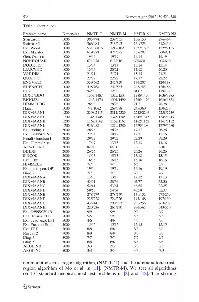
Table 1 Numerical results

Problem name Dimension NMTR-T NMTR-M NMTR-N1 NMTR-N2

Powell badly scal. 2 54/62 54/62 54/62 54/62Brown badly scal. 2 39/39 41/42 41/42 47/48Full Hessian FH1 2 30/32 30/32 19/21 29/31Full Hessian FH2 2 6/7 6/7 5/6 6/7Beale 2 14/16 14/16 12/14 14/16Ext. Hiebert 2 1906/2061 1478/1549 1622/1681 1962/2039MCCORMCK 2 10/11 10/11 10/11 10/11Helical valley 3 41/46 27/31 29/32 30/34Box three-dim. 3 28/30 27/29 26/28 27/29Gulf res. and dev. 3 50/60 64/78 58/72 36/41Gaussian 3 5/6 5/6 5/6 5/6Brown and Dennis 4 36/42 27/34 30/37 29/35Wood 4 80/86 69/77 65/75 47/52Biggs EXP6 6 160/180 139/151 163/191 266/322GENHUMPS 20 1021/1305 309/458 174/254 95/173SINQUAD 20 97/118 81/96 115/145 387/440FLETCBV3 20 6628/8120 2811/3359 2189/2589 2610/3063Watson 31 77/86 73/80 43/49 67/77Gen. tridiag. 2 40 188/264 181/263 188/267 143/228Diag. 3 40 128/161 132/182 121/157 126/180Penalty function II 100 333/408 231/291 99/136 135/188Diag. 1 100 261/343 258/356 251/340 131/198Trigonometric 500 78/88 100/110 70/79 100/110Gen. Rosenbrock 500 4659/6844 5212/7654 5112/7521 6072/8048Broyden tridiag. 500 2418/3404 1077/1738 2408/3440 1311/1862Diag. 9 500 970/1382 561/866 248/381 699/913CUBE 500 675/837 721/910 148/198 969/1341NONSCOMP 500 2084/2652 2335/3035 916/1355 2938/3720POWER 500 6982/10184 7983/11472 5398/7762 9833/13314BDQRTIC 500 443/621 174/251 116/170 108/160TRIDIA 500 3280/4886 3401/4811 2459/3563 3786/5187FLETCHCR 500 4005/5759 4505/6431 4515/6555 5473/7272Ext. tridiag. 2 1000 123/124 123/124 89/90 123/124Gen. tridiag. 1 1000 914/1318 280/412 235/341 147/228Ext. Powell sing. 1000 1765/2474 2059/3051 292/435 3010/4480Ext. Rosenbrock 1000 423/576 444/654 404/604 714/1080Partial per. quad. 1000 770/1104 235/351 225/331 123/190Almost per. quad. 1000 1044/1546 1206/1983 581/924 1374/2081Ext. block diag. 1 1000 12/13 12/13 12/13 13/15per. quad. diag. 1000 411/509 186/227 127/155 106/144Ext. quad. pen. QP2 1000 62/68 67/74 63/70 62/69Ext. White and Holst 1000 856/1186 169/221 876/1322 1398/2116Gen. White and Holst 1000 8964/12879 13428/19229 6018/8334 15807/22068Per. tridiag. Quad. 1000 1082/1582 1206/1982 596/920 1372/1981Variably dim. 1000 21/21 21/21 15/15 21/21Gen. PSC1 1000 198/212 51/54 85/97 51/54Ext. PSC1 1000 15/15 15/15 13/13 15/15Quad. QF1 1000 1063/1582 1215/1995 579/912 1431/1982Quad. QF2 1000 1386/2047 1462/2384 847/1427 1665/2477Raydan 1 1000 958/1411 1101/1791 499/806 1216/1584Diag. 2 1000 285/285 285/285 195/195 285/285Diag. 4 1000 5/5 5/5 4/4 5/5Per. quad. 1000 1070/1563 1197/1975 562/894 1350/2000Ext. Beale 1000 16/17 16/17 13/14 16/17

536 Numer Algor (2012) 59:523–540

Table 1 (continued)

Problem name Dimension NMTR-T NMTR-M NMTR-N1 NMTR-N2

Staircase 1 1000 395/478 239/335 106/150 296/404Staircase 2 1000 366/484 213/293 161/223 318/419Ext. Wood 1000 5310/6816 1217/1827 1222/1635 1529/2165Ext. Maratos 1000 619/879 474/695 465/707 560/831Gen. Quartic 1000 19/19 19/19 14/14 19/19NONDQUAR 1000 671/678 612/618 620/631 606/610DQDRTIC 1000 13/14 13/14 13/14 13/14LIARWHD 1000 13/13 20/21 12/12 20/20VARDIM 1000 21/21 21/21 15/15 21/21QUARTC 1000 22/22 22/22 17/17 22/22ENGVAL1 1000 559/762 242/329 150/207 120/168EDENSCH 1000 558/768 254/365 202/285 126/186EG2 1000 94/99 72/73 81/87 119/132DIXON3DQ 1000 1357/1487 1322/1531 1288/1476 1636/1985BIGGSB1 1000 1345/1476 1301/1490 1290/1476 1626/1872HIMMELBG 1000 28/28 28/28 21/21 28/28Hager 1000 741/1062 269/378 245/360 150/218DIXMAANI 1200 2398/2415 2311/2320 2243/2246 2258/2259DIXMAANJ 1200 1345/1345 1345/1345 1345/1345 1345/1345DIXMAANK 1200 1162/1162 1162/1162 1162/1162 1162/1162DIXMAANL 1200 956/958 1279/1280 1279/1280 1279/1280Ext. tridiag. 1 2000 26/26 26/26 17/17 26/26Ext. DENSCHNF 2000 22/24 18/19 19/21 15/16Penalty function I 2000 29/29 29/29 29/29 29/29Ext. Himmelblau 2000 17/17 13/15 13/13 14/16ARWHEAD 2000 8/10 8/10 7/9 8/10BDEXP 2000 26/26 26/26 26/26 26/26SINCOS 2000 15/15 15/15 13/13 15/15Ext. Cliff 2000 16/16 16/16 16/16 16/16HIMMELH 2000 7/7 7/7 6/6 7/7Ext. quad. pen. QP1 3000 19/19 19/19 16/16 19/19Diag. 7 3000 7/7 7/7 6/6 7/7DIXMAANA 3000 13/13 13/13 12/12 13/13DIXMAANB 3000 43/51 28/34 67/77 32/36DIXMAANC 3000 52/61 53/61 46/55 22/25DIXMAAND 3000 50/58 54/64 48/58 32/37DIXMAANE 3000 278/279 278/279 151/152 278/279DIXMAANF 3000 225/228 224/226 145/148 197/199DIXMAANG 3000 435/441 390/393 251/256 263/272DIXMAANH 3000 220/236 265/270 350/565 543/559Ext. DENSCHNB 5000 9/9 9/9 9/9 9/9Full Hessian FH3 5000 5/5 5/5 5/5 5/5Ext. quad. exp. EP1 5000 4/6 4/6 4/6 4/6Ext. Fre. and Roth 5000 15/15 15/15 15/15 15/15Ext. TET 5000 8/8 8/8 8/8 8/8Raydan 2 5000 8/8 8/8 8/8 8/8Diag. 5 5000 7/7 7/7 7/7 7/7Diag. 8 5000 6/6 6/6 6/6 6/6ARGLINB 5000 3/3 3/3 3/3 3/3ARGLINC 5000 3/3 3/3 3/3 /3/3

nonmonotone trust-region algorithm, (NMTR-T), and the nonmonotone trust-region algorithm of Mo et al. in [11], (NMTR-M). We test all algorithmson 104 standard unconstrained test problems in [2] and [12]. The starting

Numer Algor (2012) 59:523–540 537

points are the standard ones provided by these literatures. We performed ourcodes in double precision arithmetic format in MATLAB 7.4 programmingenvironment on a 3.0 GHz Intel single-core processor computer with 1GB ofRAM. For proper comparison, we provide all codes in the same subroutineand solved the trust-region subproblems by Steihaug–Toint procedure (see p.205 in [4]).

In all algorithms, we set μ1 = 0.05, μ2 = 0.9 and δ0 = 10. In addition, thestopping criterion is

‖∇ f (xk)‖ ≤ 10−6‖∇ f (x0)‖.

We choose N = 10 for the new algorithm and the NMTR-T. Based on ourpreliminary numerical experiments, we decided to update ηk by

ηk ={

η0/2, if k = 1;(ηk−1 + ηk−2)/2, if k ≥ 2.

We name our algorithm as NMTR-N1 and NMTR-N2 whenever η0 = 0.85and η0 = 0.2, respectively. For NMTR-M algorithm, we select η0 = 0.85 as

1 1.5 2 2.5 3 3.5 4 4.5 5 5.50.2

0.3

0.4

0.5

0.6

0.7

0.8

0.9

1

NMTR- TNMTR- MNMTR- N1NMTR- N2

Fig. 1 Performance profile for the number of iterates

538 Numer Algor (2012) 59:523–540

considered in [8, 11]. For all algorithms, the trust-region radius update isimplemented using

δk+1 =⎧⎨

⎩

c1‖dk‖, if r̂k < μ1;δk, if μ1 ≤ r̂k < μ2;max [δk, c2‖dk‖], if r̂k ≥ μ2,

where c1 = 0.25 and c2 = 2.5. Table 1 shows the total number of iterates (ni)and the total number of function evaluations (n f ) that each algorithm need tosolve an arbitrary problem. In Table 1, we have only kept the problems forwhich all algorithms converge to the same local solution.

In order to compare iterative algorithms, Dolan and Moré in [7] proposeda new technique employing a statistical process by demonstration of a per-formance profile. In this technique, one can choose a performance index asmeasure of comparison among the considered algorithms and can illustrate theresults with a performance profile. Figures 1 and 2 show this process with indexof the number of iterates and the number of function evaluations, respectively.

In Fig. 1, firstly, we observe that NMTR-N1 have the most wins while itsolves about 70% of the tests with the greatest efficiency. Moreover, if wefocus our attention on the ability of completing a run successfully, we haveagain that NMTR-N1 is the best among considered algorithms. Secondly,

1 1.5 2 2.5 3 3.5 4 4.5 5 5.5

0.4

0.5

0.6

0.7

0.8

0.9

1

NMTR- TNMTR- MNMTR- N1NMTR- N2

Fig. 2 Performance profile for the number of function evaluations

Numer Algor (2012) 59:523–540 539

NMTR-N2 is competitive with NMTR-M, but in most cases it grows up muchfaster than NMTR-M. Finally, one can see that NMTR-N1 increase noticeablyin comparison with the other considered algorithms. It means that in the casesthat NMTR-N1 is not the best algorithm which performance index is close tothe performance index of the best algorithm. Therefore, we can deduce thatthe new algorithm is more efficient and robustness than the other consideredtrust-region algorithms in the sense of the total number of iterates.

Results of Fig. 2 are remarkably similar to the mentioned results of Fig. 1,in the sense of the total number of function evaluations.

5 Conclusions

The present paper proposes a new nonmonotone strategy and exploits it intrust-region framework to introduce an efficient procedure to solve uncon-strained optimization. The new nonmonotone strategy has been constructedbased on appropriate using of the function value in current iterate to overcomesome disadvantages of traditional nonmonotone strategy. In addition, anadaptive process for increasing the effects of traditional nonmonotone term farfrom the optimum and decreasing its effects close to the optimum is suggested.The global convergence to first-order and second-order stationary points forthe new algorithm, similar to those stated for common trust-region algorithm,have been established. Preliminary numerical results show the significantefficiency of the new algorithm.

Acknowledgements The authors would like to thank the referees for their valuable suggestionsand comments.

References

1. Ahookhosh, M., Amini, K.: A nonmonotone trust region method with adaptive radius forunconstrained optimization. Comput. Math. Appl. 60, 411–422 (2010)

2. Andrei, N.: An unconstrained optimization test functions collection. Adv. Model. Optim.10(1), 147–161 (2008)

3. Chamberlain, R.M., Powell, M.J.D., Lemarechal, C., Pedersen, H.C.: The watchdog techniquefor forcing convergence in algorithm for constrained optimization. Math. Program. Stud. 16,1–17 (1982)

4. Conn, A.R., Gould, N.I.M., Toint, Ph.L.: Trust-Region Methods. Society for Industrial andApplied Mathematics (SIAM), Philadelphia (2000)

5. Dai, Y.H.: On the nonmonotone line search. J. Optim. Theory Appl. 112(2), 315–330 (2002)6. Deng, N.Y., Xiao, Y., Zhou, F.J.: Nonmonotonic trust region algorithm. J. Optim. Theory

Appl. 76, 259–285 (1993)7. Dolan, E., Moré, J.J.: Benchmarking optimization software with performance profiles. Math.

Program. 91, 201–213 (2002)8. Gould, N.I.M, Orban, D., Sartenaer, A., Toint, Ph.L.: Sentesivity of trust-region algorithms to

their parameters. Q. J. Oper. Res. 3, 227–241 (2005)9. Grippo, L., Lampariello, F., Lucidi, S.: A nonmonotone line search technique for Newton’s

method. SIAM J. Numer. Anal. 23, 707–716 (1986)

540 Numer Algor (2012) 59:523–540

10. Grippo, L., Lampariello, F., Lucidi, S.: A truncated Newton method with nonmonotone line-search for unconstrained optimization. J. Optim. Theory Appl. 60, 401–419 (1989)

11. Mo, J., Liu, C., Yan, S.: A nonmonotone trust region method based on nonincreasing tech-nique of weighted average of the succesive function value. J. Comput. Appl. Math. 209, 97–108(2007)

12. Moré, J.J., Garbow, B.S., Hillstrom, K.E.: Testing unconstrained optimization software. ACMTrans. Math. Softw. 7, 17–41 (1981)

13. Nocedal, J., Yuan, Y.: Combining trust region and line search techniques. In: Yuan, Y. (ed.)Advanced in Nonlinear Programming, pp. 153–175. Kluwer Academic, Dordrecht (1996)

14. Nocedal, J., Wright, S.J.: Numerical Optimization. Springer, New York (2006)15. Panier, E.R., Tits, A.L.: Avoiding the Maratos effect by means of a nonmonotone linesearch.

SIAM J. Numer. Anal. 28, 1183–1195 (1991)16. Powell, M.J.D.: Convergence properties of a class minimization algorithms. In: Mangasarian,

O.L., Meyer, R.R., Robinson, S.M. (eds.) Nonlinear Programming, vol. 2, pp. l–27. Academic,New York (1975)

17. Powell, M.J.D.: On the global convergence of trust region algorithms for unconstrained opti-mization. Math. Program. 29, 297–303 (1984)

18. Schultz, G.A., Schnabel, R.B., Byrd, R.H.: A family of trust-region-based algorithms forunconstrained minimization with strong global convergence. SIAM J. Numer. Anal. 22,47–67 (1985)

19. Toint, Ph.L.: An assessment of nonmonotone linesearch technique for unconstrained opti-mization. SIAM J. Sci. Comput. 17, 725–739 (1996)

20. Toint, Ph.L.: Non-monotone trust-region algorithm for nonlinear optimization subject toconvex constraints. Math. Program. 77, 69–94 (1997)

21. Xiao, Y., Zhou, F.J.: Nonmonotone trust region methods with curvilinear path in uncon-strained optimization. Computing 48, 303–317 (1992)

22. Xiao, Y., Chu, E.K.W.: Nonmonotone trust region methods. Technical Report 95/17, MonashUniversity, Clayton, Australia (1995)

23. Zhang, H.C., Hager, W.W.: A nonmonotone line search technique for unconstrained optimiza-tion. SIAM J. Optim. 14(4), 1043–1056 (2004)

24. Zhou, F., Xiao, Y.: A class of nonmonotone stabilization trust region methods. Computing53(2), 119–136 (1994)