An Evaluation of the Hybrid Sparse/Diffuse Algorithm

for Underwater Acoustic Channel Estimation

Nicolò Michelusi∗, Beatrice Tomasi∗, Urbashi Mitra†, James Preisig‡, and Michele Zorzi∗∗Department of Information Engineering — University of Padova, Italy

†Ming Hsieh Department of Electrical Engineering — University of Southern California, (CA) USA‡Department of Applied Ocean Physics and Engineering — Woods Hole Oceanographic Institution, (MA) USA

Email: michelusi@dei.unipd.it, tomasibe@dei.unipd.it, ubli@usc.edu, jpreisig@whoi.edu, zorzi@dei.unipd.it

Abstract—The underwater acoustic channel has been

usually modeled as sparse. However, in some scenarios

of interest, e.g., shallow water environments due to the

interaction with the surface and the seabed, the channel

exhibits also a dense arrival of multipath components.

In these cases, a Hybrid Sparse/Diffuse (HSD) channel

representation, rather than a purely sparse one, may be

more appropriate.

In this work, we present the HSD channel model

and channel estimators based on it. We evaluate these

estimation strategies on the SPACE08 experimental data

set. We show that the HSD estimators outperform the more

conventional purely sparse and least squares estimators.

Moreover, we show that an exponential Power Delay Profile

(PDP) for the diffuse component is appropriate in scenarios

where the receiver is far away from the transmitter.

Finally, the HSD estimators and the exponential PDP

model are shown to be robust even in scenarios where

the channel does not exhibit a diffuse component.

I. INTRODUCTION

UnderWater Acoustic (UWA) communication is

emerging as a technology for applications such as en-

vironmental monitoring, marine surveillance and ocean

exploration [1], [2].

UWA channels exhibit challenging characteristics such

as high attenuation, large channel delay spread, Doppler

spread [3], [4] and, consequently, incur low through-

put and reliability [5], relative to wireless terrestrial

radiofrequency channels. In particular, the large delay

spread causes intersymbol interference (ISI), which can

be compensated by equalization of the received se-

quence. However, the performance of coherent equalizers

is highly sensitive to the availability of accurate channel

estimates. To this end, it is crucial to develop channel

estimation strategies that exploit the intrinsic nature of

UWA propagation to improve the estimation accuracy.

Due to the large inter-arrival delays of multipath com-

ponents, relative to the delay resolution at the receiver,

the UWA channel can be represented by sparse specular

arrivals that can be predicted by geometrically based

ray-tracing algorithms, such as Bellhop [6], once the

environmental conditions are known. For this reason,

several UWA channel estimators based on sparse approx-

imations and compressed sensing have been proposed

and successfully employed in the literature [7]–[10]. In

[11], a comparative study among purely sparse and Least

Squares (LS) channel estimators has been performed,

showing that the former, while improving the estimation

accuracy when the channel is truly sparse, are robust

even when the channel does not exhibit a sparse nature.

However, in many scenarios of interest in UWA com-

munications, e.g., shallow water environments, where the

reflections of the sound waves from the seabed and sea

surface give rise to a richer interaction among multi-

path components, also a dense UWA channel has been

observed. For these scenarios, a purely sparse model

does not appropriately represent the channel behavior. In

[12] it is shown that shallow-water propagation channels

exhibit high variability, ranging from stable single-path

propagation to overspread, and from sparse to densely

populated impulse responses. This is caused by the rough

surface scattering and by inhomogeneities in the water

column, which induce different angles of arrival of the

multipath components that superimpose at the receiver

according to constructive and destructive interference

patterns.

Although robust [11], channel estimators based on

the assumption of a purely sparse channel are not ex-

pected to perform well when the channel is not purely

sparse. For this reason, it is crucial to design channel

estimation strategies attaining high accuracy even in

the scenarios where the channel exhibits a dense, or a

hybrid sparse/dense, structure. In this paper, we study

the application to UWA channels of a novel Hybrid

Sparse/Diffuse (HSD) model, originally proposed in [13]

for Ultra-Wide Band (UWB) systems. This model com-

bines both a diffuse component, to model the multipath

0-933957-39-8 ©2011 MTS

fading arising in dense multipath scenarios, and a sparse

component, to model the fine-grained delay resolution

at the receiver relative to the interarrival time of the

resolvable multipath components. Moreover, we propose

to use an exponential Power Delay Profile (PDP) for the

diffuse component, and measure how this model fits the

sample PDP measured from a representative subset of

the SPACE08 data set. On the same data set, we then

evaluate the Mean Squared Error (MSE) accuracy for

the prediction of the observed sequence attained by HSD

channel estimators; we compare our new estimators with

conventional purely sparse and LS estimators.

We show that the assumption of an exponential PDP

is accurate in shallow water environments where the

receiver is far away from the transmitter, whereas a

clustered model, according to which the channel is

characterized by few strong, resolvable arrivals, each fol-

lowed by a cluster of weaker arrivals, is more appropriate

when the receiver is closer to the transmitter. Channel

estimation strategies based on the HSD model and on the

exponential PDP model for the diffuse component attain

a better estimation accuracy than conventional LS based

and purely sparse estimators, in scenarios where the

exponential PDP model fits well the observed behavior of

the diffuse component. Nevertheless, these estimators are

found to be robust even in scenarios where the measured

UWA channel does not exhibit an exponential PDP shape

or a diffuse nature.

The paper is organized as follows. In Section II, we

review the state of the art in UWA channel modeling, and

we discuss the importance of employing a HSD model

for the purpose of UWA channel estimation. In Section

III, we present the system model and the HSD channel

model. In Section IV, we design estimators specific to

the HSD model, namely the Generalized Thresholding

and the Generalized MMSE estimators. These estimators

are evaluated on the SPACE08 experimental data set.

Given that we assume an exponential PDP for the diffuse

component, in Section V we show experimental results

for the fitting of the exponential PDP model to the data.

In Section VI, we provide numerical results and compare

the prediction accuracy achieved by conventional purely

sparse, LS estimators and the novel HSD estimators

based on the exponential PDP model for the diffuse

component. Finally, in Section VII we conclude the

paper.

A. Notation

We use lower-case bold letters for column vectors (a),

and upper-case bold letters for matrices (A). The scalar

a(k) denotes the kth entry of vector a, and Ak,j denotes

the (k, j)th entry of matrix A. The matrix A∗ is the

transpose, complex conjugate of A. The vector a ⊙ b

is the component-wise (Schur) product of vectors a and

b. The circular Gaussian distribution with mean m and

covariance Σ is denoted by CN (m,Σ). The Bernoulli

distribution with parameter q is given by B(q). The

indicator function is denoted by I (·). The expectation of

random variable x, conditioned on y is written as E [x|y].

II. UNDERWATER ACOUSTIC CHANNEL MODELING

In this section, we review current channel models for

UWA communications, and we present a novel Hybrid

Sparse/Diffuse (HSD) model, originally proposed for

UWB channels in [13]–[15]. This model, while retaining

key physical features of the channel, lends itself to the

design of estimators.

In the literature, we can broadly classify UWA chan-

nel modeling efforts into a deterministic approach and

a statistical approach. The former aims to develop a

static model, which is able to replicate the multipath

arrival delays and amplitudes, once the environmental

conditions are known. In this category, we include [16]–

[18], which present studies of the physics involved in

the interaction of sound waves with water conditions,

the water bottom and surface. Of particular interest is the

Bellhop tool [6], a ray-tracing algorithm which is able to

predict the multipath arrival pattern of the channel, once

the environmental conditions are known. The statistical

approach tries to identify an accurate statistical model

for the UWA channel, which can be used to develop

and enhance signal processing techniques and algorithms

for communications systems [5], [19]–[23]. In particular,

these studies investigate the second order and complete

statistics of the UWA channel impulse response in order

to derive a suitable and realistic model for simulation

studies and performance analysis.

While these models are important for realistic perfor-

mance assessment, the full exploitation of the determin-

istic and statistical properties in the design of channel

estimation techniques can be complex. For this reason,

in this paper we seek a simplified channel model as a

reference for the design of channel estimation strategies.

Due to the relatively slow propagation speed of sound

waves in water (∼ 1.5 km/s), propagation path length

differences of only a few meters can result in delays of

a few milliseconds between arrivals. With typical signal

bandwidths on the order of 5 kHz in mid-frequency sys-

tems, such delays between arrivals are easily resolvable

and can result in a sparse multipath structure.

However, in many scenarios of interest in UWA com-

munications, e.g., shallow water environments, a sparse

channel structure is not sufficient to describe other UWA

propagation mechanisms, e.g., diffuse (dense) scattering,

diffraction effects and frequency dispersion, which are

better represented by a dense channel. We thus propose

a novel HSD model, which views the channel as the

superposition of two independent components: the sparse

component, which models the resolvable multipath sig-

nals, owing to the fine delay resolution, and the diffuse

component, which models other propagation phenomena

that cannot be described by a sparse structure, such

as dense scattering and frequency dispersion of UWA

channels.

The HSD channel model is presented in detail in the

following section.

III. SYSTEM MODEL

We consider a point-to-point Underwater Acoustic

channel. The source transmits a sequence of M pilot

symbols, x(n), n = −(L − 1), . . . ,M − L, over a

channel h(l), l = 0, . . . , L− 1 with known delay spread

L ≥ 1. The received discrete-time, baseband signal

over the corresponding observation interval of length

N = M − L+ 1, is given by

y(n) =

L−1∑

l=0

h(l)x(n− l) + w(n), n = 0, . . . , N − 1,

where w(n) ∈ CN (0, σ2w) is iid circular Gaussian noise.

By collecting the N received, noise and channel samples

in the column vectors y = [y(0), y(1), . . . , y(N − 1)]T ,w = [w(0), w(1), . . . , w(N − 1)]T ∈ CN and h =[h(0), h(1), . . . , h(L− 1)]T ∈ CL, respectively, and let-

ting X ∈ CN×L be the N×L Toeplitz matrix associated

with the pilot sequence, with the vector of the transmitted

pilot sequence [x(−i), x(1− i), . . . , x(N − 1− i)]T as

its ith column, i = 0, . . . , L− 1, we have the following

matrix representation:

y = Xh+w. (1)

The discrete baseband channel vector h is modeled

according to the HSD model developed in [13], [14] for

UWB systems, i.e.,

h = as ⊙ cs + hd, (2)

where as ⊙ cs is the sparse component, and hd is

the diffuse component. In particular, as ∈ {0, 1}L is

the sparsity pattern, whose entries are equal to one in

the positions corresponding to the resolvable multipath

components, and zero otherwise; its entries are drawn iid

from B(q), where q ≪ 1 so as to enforce sparsity. Notice

that the smaller q, the sparser the sparse component

as ⊙ cs is expected to be. The sparse coefficient vector

cs is modeled as a deterministic and unknown vector.

Finally, we use the Rayleigh fading approximation for

the diffuse component, hd ∼ CN (0,Λd), where Λd

is diagonal, with diagonal entries given by the PDP

Pd(k), k = 0, . . . , L− 1.

Remark 1. We assume that cs is a deterministic and

unknown vector, because the statistics of the specular

components, that vary according to the large scale fading,

are usually difficult to estimate. On the other hand, the

Rayleigh fading assumption for the diffuse component is

consistent with the fact that it arises from the contribu-

tion of multiple paths in a single resolvable delay bin. Its

amplitude and phase vary according to the small scale

fading. Its PDP can be accurately estimated by averaging

the fading over subsequent realizations of the fading

process. This information may then be used to estimate

the channel via the linear Minimum Mean Squared Error

(MMSE) estimator [24], which improves the accuracy

over LS.

Notice that the LS estimate is a sufficient statistic for

the channel. Therefore, we will refer to the following

sufficient observation model

hLS = (X∗X)−1X∗y = h+ n, (3)

where n ∼ CN(

0, σ2w (X∗X)−1

)

. In the following,

we let σ2LS(k) = σ2

w

[

(X∗X)−1]

k,k. This represents

the variance of the noise on the kth sample of the LS

estimate. Therefore, we have n(k) ∼ CN (0, σ2LS(k)).

IV. HYBRID SPARSE/DIFFUSE CHANNEL ESTIMATORS

In [13], [14] we developed a three-step channel esti-

mator based on the HSD model presented in the previous

section:

1) The sparse coefficient vector cs is estimated via

LS, giving the estimate cs = hLS .

2) The sparsity pattern as is estimated via either

MMSE or Maximum A Posteriori (MAP) [24],

giving the estimate as.

3) The diffuse component hd is estimated via MMSE,

based on the residual estimation error after remov-

ing the estimated sparse component, (1 − as) ⊙hLS .

The overall estimate of the HSD channel is then given

by

h(k) = as(k)hLS + (1− as(k))Pd(k)

Pd(k) + σ2LS(k)

hLS ,

where Pd(k) is an estimate of Pd(k). We have two

different estimators, depending on whether MAP or

MMSE is used to estimate the sparsity pattern as. Letting

α = ln(

1−qq

)

, where q ∈ (0, 1) is an algorithm

parameter, the Generalized MMSE (G-MMSE) estimator

computes a MMSE estimate of as, given by

aMMSEs (k) =

1

1 + eα exp{

− |hLS(k)|2

Pd(k)+σ2

LS(k)

} . (4)

On the other hand, the Generalized Thresholding (G-

Thres) estimator computes a MAP estimate of as, given

by

aMAPs (k) =I

{

|hLS(k)|2 > α(

Pd(k) + σ2LS(k)

)}

.

(5)

This solution determines a thresholding of the LS es-

timate, hence the name. The intuitive idea behind the

G-Thres estimator is that the LS samples sufficiently

above the "noise" floor, represented by the sum of

the strengths of the noise and diffuse components, are

regarded as active sparse components, whose coefficients

are estimated via LS, whereas the LS samples below

this level are regarded as diffuse components and are

estimated via MMSE. A similar intuition holds for the

G-MMSE estimator.

The parameter q is the true Bernoulli parameter for

as, in contrast q is the value assumed for the estimation

phase [14], [15], which might be different from the

true parameter. Moreover, using q < q improves the

MSE estimation accuracy over using the true q, in the

asymptotic low and high Signal to Noise Ratio (SNR)

regimes [15]. Knowledge of the parameter q is thus not

crucial, since a conservative approach in the estimation

of the sparse component usually improves the estimation

accuracy.

V. POWER DELAY PROFILE MODELING

In this section, we model the PDP of the diffuse

component. In particular, we assume an exponential PDP,

and we measure the fitting of this model to the sample

PDP estimated from the data, based on the SPACE08

data set. For more details on this data set, we refer

the interested reader to [25]. In particular, we consider

two different receivers, S3 and S5, located at 200m and

1000m distance from the transmitter, respectively. The

environment can be classified as shallow water, since the

seabed is 15m below the sea surface.

The source transmits a pseudo-noise sequence of

length 60 s, with symbols drawn from {−1, 1} at rate

6510 symbols/s. The corresponding received sequence

is divided into sub-sequences of length 30ms each,

corresponding to N = 194 samples. Let y(i) be the

observation vector from the ith sub-sequence, and X(i)

be the Toeplitz matrix associated with the corresponding

pilot sequence. A time series of LS channel estimates

with delay spread 15ms (L = 97 samples) is generated

as h(i)LS =

(

X(i)∗X(i))−1

X(i)∗y(i). This time series

therefore represents the samples of the time-varying

channel spaced in time 30ms apart.The sample PDP is computed by averaging over

Nch = 1878 subsequent channel realizations, corre-

sponding to an observation window of 56 s. We have

Psample(k) =1

Nch

Nch−1∑

i=0

∣

∣

∣h(i)LS(k)

∣

∣

∣

2. (6)

We now evaluate the exponential model for the PDP

of the diffuse component, and we compare it with the

sample PDP estimated from the data. At this point, since

we are not assuming any a priori model for the PDP, and

therefore we cannot distinguish the specular components

from the diffuse background, which is unknown, we keep

the sparse component to compute the sample PDP and

the exponential fitting.

Let Pd(k) = βe−ωk, k = 0, . . . , L − 1 be the

exponential PDP as a function of the channel delay. This

is parameterized by the power β, and the decay ω. Noticethat lnPd(k) = lnβ − ωk = ρ − ωk, where we have

defined ρ = lnβ. These parameters can be estimated

by computing a linear fitting of ln Psample(k), i.e., bysolving

{ρ, ω} = argminρ,ω

∑

k

∣

∣

∣ln Psample(k)− ρ+ ωk

∣

∣

∣

2. (7)

We then determine the fitting error of the estimated

exponential PDP with the sample PDP estimate as

f(

Psample

)

=∑

k

∣

∣

∣ln Psample(k)− ρ+ ωk

∣

∣

∣

2. (8)

Figure 1 shows the fitting error for the two receivers

S3 and S5, respectively, over a representative subset of

the SPACE08 data set. We notice that S5, which is

the receiver farther away from the transmitter, fits the

exponential PDP better than receiver S3. This may be

0 5 10 15 200

0.05

0.1

0.15

0.2

0.25

0.3

file index

Mean s

quare

fitting e

rror

S3, 200 m

S5, 1000 m

Figure 1: Fitting error of the sample PDP, estimated from the

data, to the exponential PDP. The smaller the error, the better

the fitting of the sample PDP to the exponential model.

�� �����

�

��

�

Figure 2: A shallow water scenario, with the line of sight

component, and two echoes reflected by the seabed and the

water surface.

due to a multiplicative loss at each water surface or

bottom bounce and an exponential absorption loss of the

propagation medium.

Figure 3 shows a typical diffuse PDP for receivers

S3 and S5, respectively. We observe that receiver S5

exhibits a more diffuse channel than receiver S3, and

a good fitting to the exponential model. On the other

hand, for receiver S3 a clustered model, where few

strong resolvable multipath components are followed

by a cluster of arrivals, seems more appropriate. This

behavior can be interpreted with the help of Figure 2,

which represents a shallow water scenario with the line

of sight component and two echoes reflected by the

seabed and the water surface, respectively.

Let dTR be the distance between transmitter and re-

ceiver, hT the depth of the transmitter/receiver pair below

the sea level, hB their height above the seabed, and

c ≃ 1.5 km/s the speed of the sound wave in the water.

The line of sight component reaches the receiver with a

delay dTR

c. The echo reflected by the sea surface reaches

the receiver with a delay

√d2

TR+4h2

T

c, ideally assuming

0 5 10 15−3.5

−3

−2.5

−2

−1.5

−1

−0.5

0

channel delay [ms]

Lo

ga

rith

m o

f th

e a

ve

rag

e P

ow

er

De

lay P

rofile

(P

DP

)

Sample estimate

EM algorithm estimate

linear fitting

(a) Receiver S3

0 5 10 15−5.5

−5

−4.5

−4

−3.5

−3

channel delay [ms]

Lo

ga

rith

m o

f th

e a

ve

rag

e P

ow

er

De

lay P

rofile

(P

DP

)

Sample estimate

EM algorithm estimate

linear fitting

(b) Receiver S5

Figure 3: A typical sample PDP for receivers S3 and S5, with

the exponential PDP estimated by linear fitting, and the PDP

estimate based on the EM algorithm [14].

that the reflection occurs at distance dTR

2 from the source

(a similar expression holds for the echo reflected by the

seabed). Therefore, the interarrival time between the line

of sight and the echo reflected by the sea surface is given

by τinter(dTR) =

√d2

TR+4h2

T−dTR

c, which is a decreasing

function of dTR. Therefore, the further away the receiver

from the transmitter, the smaller the interarrival time,

the richer the interaction of the multipath components,

and the more diffuse the nature exhibited by the UWA

channel.

VI. NUMERICAL RESULTS

We now present some numerical results, and we com-

pare the mean squared prediction error of the received

sequence using HSD, LS, and a purely sparse estimator,

−30 −20 −10 0 10 20 30 40 5010

−1

100

101

102

103

104

105

SNR [dB]

MS

E

G−Thres dataG−Thres modelLSSparse

(a) Entire SNR range

−5 0 5 10 15 20 25 30

100

101

102

SNR [dB]

MS

E

G−Thres dataG−Thres modelLSSparse

(b) Zoom in medium SNR range

Figure 4: Mean squared prediction error of the observed

sequence for receiver S3, G-Thres estimator.

as a function of the SNR. In order to generate all

the SNR values of interest, we add the UWA noise

sequence w(i), scaled by a factor√S−1

> 0, to the

received sequence y(i) in the estimation phase, so as to

induce SNR dependent channel estimation errors. Letting

h(i) be the ith channel estimate, estimated from the

noisy received sequence y(i)+√S−1

w(i), y(i+1) be the

observed sequence that we want to predict, and X(i+1)

be the Toeplitz matrix associated with the corresponding

pilot sequence, the MSE for the prediction of y(i+1) is

defined as

E

[

∥

∥

∥y(i+1) −X(i+1)h(i)

∥

∥

∥

2

2

]

, (9)

where the expectation is computed with respect to the

realizations of the noise (intrinsic noise in the experi-

mental data set and additional noise w(i)) and of the

−30 −20 −10 0 10 20 30 40 5010

−1

100

101

102

103

104

105

SNR [dB]

MS

E

G−Thres dataG−Thres modelLSSparse

(a) Entire SNR range

−5 0 5 10 15 20 25 30

100

101

102

SNR [dB]

MS

E

G−Thres dataG−Thres modelLSSparse

(b) Zoom in medium SNR range

Figure 5: Mean squared prediction error of the observed

sequence for receiver S5, G-Thres estimator.

channel. The overall mean squared prediction error is

computed by averaging the sample squared error term∥

∥

∥y(i+1) −X(i+1)h(i)

∥

∥

∥

2

2over the sub-sequence index i,

and over multiple received sequences, each 60 s long,

collected over different times and environmental condi-

tions.

For the HSD model, we consider the G-Thres esti-

mator, with α = ln(

1−qq

)

, q = 0.001. For the sake

of clarity of exposition, we provide the results for the

G-Thres and G-MMSE estimators in separate figures.

Moreover, we discuss the results only for the G-Thres

estimator, since the same considerations hold for the G-

MMSE estimator. We consider two different cases for

the estimate of the PDP of the diffuse component: the

sample PDP estimate, averaged over Nch = 1878 subse-

−30 −20 −10 0 10 20 30 40 5010

−1

100

101

102

103

104

105

SNR [dB]

MS

E

G−MMSE dataG−MMSE modelLSSparse

(a) Entire SNR range

−5 0 5 10 15 20 25 30

100

101

102

SNR [dB]

MS

E

G−MMSE dataG−MMSE modelLSSparse

(b) Zoom in medium SNR range

Figure 6: Mean squared prediction error of the observed

sequence for receiver S3, G-MMSE estimator.

quent channel realizations, corresponding to a temporal

window of 56 s; and the exponential PDP model, based

on only one channel realization. In the latter case, we

employ the Expectation-Maximization (EM) algorithm

[26] developed in [14], which exploits the HSD structure

of the channel to jointly estimate the sparse and diffuse

components, and the power β and decay rate ω of

the exponential PDP of the diffuse component. One

realization of the channel is sufficient in this case, due

to the structure of the PDP which makes it possible to

average the fading over the delay dimension, rather than

over subsequent channel realizations.

As to the purely sparse case, we employ the G-Thres

estimator assuming no diffuse component, to allow a fair

comparison with the HSD model. This estimator, due

to its thresholding operation, generates a sparse channel

−30 −20 −10 0 10 20 30 40 5010

−1

100

101

102

103

104

105

SNR [dB]

MS

E

G−MMSE dataG−MMSE modelLSSparse

(a) Entire SNR range

−5 0 5 10 15 20 25 30

100

101

102

SNR [dB]

MS

E

G−MMSE dataG−MMSE modelLSSparse

(b) Zoom in medium SNR range

Figure 7: Mean squared prediction error of the observed

sequence for receiver S5, G-MMSE estimator.

structure.

Figures 4 and 5 show the mean squared prediction

error for receivers S3 and S5 for the G-Thres estimator,

respectively. In particular, the labels "G-Thres data" and

"G-Thres model" refer to the G-Thres estimators using

the sample estimate of the PDP of the diffuse component

and the exponential PDP model, respectively.

We notice that both the G-Thres and the sparse esti-

mators perform better than LS, as observed in [7], [8],

[11] for other sparse estimators. Moreover, in the low

SNR region the G-Thres and the purely sparse estimators

achieve the same prediction error. In fact, in this region,

the diffuse component hd is below the noise floor, and

cannot thus be distinguished from the noise. Therefore,

an accurate estimate of hd is not possible in this regime,

and the HSD model does not bring any advantage over

0 5 10 150

0.1

0.2

0.3

0.4

0.5

0.6

0.7

channel delay [ms]

|h|

Sparse component

Diffuse component

sqrt of PDP of diffuse comp.

(a) SNR=10dB

0 5 10 150

0.05

0.1

0.15

0.2

0.25

0.3

0.35

0.4

channel delay [ms]

|h|

Sparse component

Diffuse component

sqrt of PDP of diffuse comp.

(b) SNR=50dB

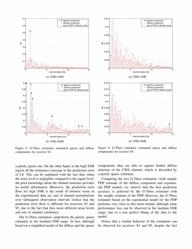
Figure 8: G-Thres estimator, estimated sparse and diffuse

components for receiver S3.

a purely sparse one. On the other hand, in the high SNR

region all the estimators converge to the prediction error

of LS. This can be explained with the fact that, when

the noise level is negligible compared to the signal level,

the prior knowledge about the channel structure provides

no useful information. Moreover, the prediction error

floor for high SNR is the result of intrinsic noise in

the experimental data set, and of channel perturbations

over subsequent observation intervals (notice that the

prediction error floor is different for receivers S3 and

S5, due to the fact that they incur different noise levels

and rate of channel variations).

The G-Thres estimators outperform the purely sparse

estimator in the medium SNR range. In fact, although

based on a simplified model of the diffuse and the sparse

0 5 10 150

0.002

0.004

0.006

0.008

0.01

0.012

channel delay [ms]

|h|

Sparse component

Diffuse component

sqrt of PDP of diffuse comp.

(a) SNR=10dB

0 5 10 150

0.002

0.004

0.006

0.008

0.01

0.012

0.014

0.016

channel delay [ms]

|h|

Sparse component

Diffuse component

sqrt of PDP of diffuse comp.

(b) SNR=50dB

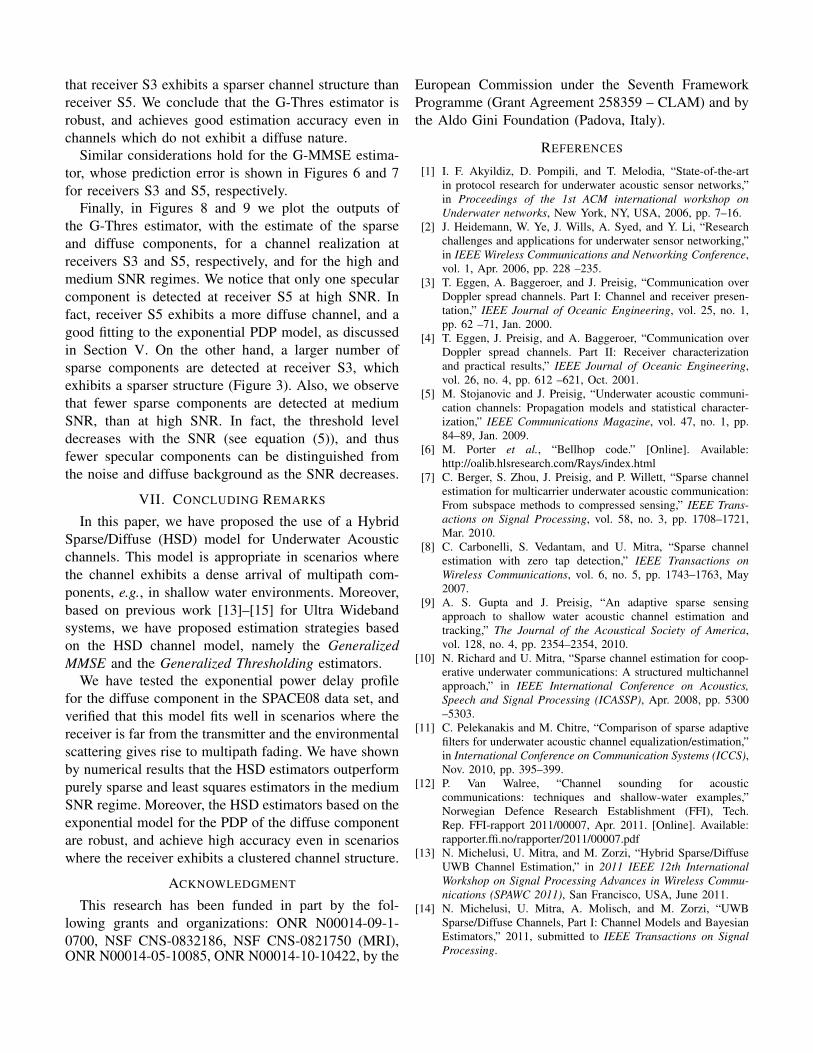
Figure 9: G-Thres estimator, estimated sparse and diffuse

components for receiver S5.

components, they are able to capture further diffuse

structure of the UWA channel, which is discarded by

a purely sparse estimator.

Comparing the two G-Thres estimators (with sample

PDP estimate of the diffuse component and exponen-

tial PDP model), we observe that the best prediction

accuracy is achieved by the G-Thres estimator with

the sample estimate of the PDP. However, the G-Thres

estimator based on the exponential model for the PDP

performs very close to this lower bound, although some

performance loss can be observed in the medium SNR

range, due to a non perfect fitting of the data to the

model.

Notice that a similar behavior of the estimators can

be observed for receivers S3 and S5, despite the fact

that receiver S3 exhibits a sparser channel structure than

receiver S5. We conclude that the G-Thres estimator is

robust, and achieves good estimation accuracy even in

channels which do not exhibit a diffuse nature.

Similar considerations hold for the G-MMSE estima-

tor, whose prediction error is shown in Figures 6 and 7

for receivers S3 and S5, respectively.

Finally, in Figures 8 and 9 we plot the outputs of

the G-Thres estimator, with the estimate of the sparse

and diffuse components, for a channel realization at

receivers S3 and S5, respectively, and for the high and

medium SNR regimes. We notice that only one specular

component is detected at receiver S5 at high SNR. In

fact, receiver S5 exhibits a more diffuse channel, and a

good fitting to the exponential PDP model, as discussed

in Section V. On the other hand, a larger number of

sparse components are detected at receiver S3, which

exhibits a sparser structure (Figure 3). Also, we observe

that fewer sparse components are detected at medium

SNR, than at high SNR. In fact, the threshold level

decreases with the SNR (see equation (5)), and thus

fewer specular components can be distinguished from

the noise and diffuse background as the SNR decreases.

VII. CONCLUDING REMARKS

In this paper, we have proposed the use of a Hybrid

Sparse/Diffuse (HSD) model for Underwater Acoustic

channels. This model is appropriate in scenarios where

the channel exhibits a dense arrival of multipath com-

ponents, e.g., in shallow water environments. Moreover,

based on previous work [13]–[15] for Ultra Wideband

systems, we have proposed estimation strategies based

on the HSD channel model, namely the Generalized

MMSE and the Generalized Thresholding estimators.

We have tested the exponential power delay profile

for the diffuse component in the SPACE08 data set, and

verified that this model fits well in scenarios where the

receiver is far from the transmitter and the environmental

scattering gives rise to multipath fading. We have shown

by numerical results that the HSD estimators outperform

purely sparse and least squares estimators in the medium

SNR regime. Moreover, the HSD estimators based on the

exponential model for the PDP of the diffuse component

are robust, and achieve high accuracy even in scenarios

where the receiver exhibits a clustered channel structure.

ACKNOWLEDGMENT

This research has been funded in part by the fol-

lowing grants and organizations: ONR N00014-09-1-

0700, NSF CNS-0832186, NSF CNS-0821750 (MRI),ONR N00014-05-10085, ONR N00014-10-10422, by the

European Commission under the Seventh Framework

Programme (Grant Agreement 258359 – CLAM) and by

the Aldo Gini Foundation (Padova, Italy).

REFERENCES

[1] I. F. Akyildiz, D. Pompili, and T. Melodia, “State-of-the-art

in protocol research for underwater acoustic sensor networks,”

in Proceedings of the 1st ACM international workshop on

Underwater networks, New York, NY, USA, 2006, pp. 7–16.

[2] J. Heidemann, W. Ye, J. Wills, A. Syed, and Y. Li, “Research

challenges and applications for underwater sensor networking,”

in IEEE Wireless Communications and Networking Conference,

vol. 1, Apr. 2006, pp. 228 –235.

[3] T. Eggen, A. Baggeroer, and J. Preisig, “Communication over

Doppler spread channels. Part I: Channel and receiver presen-

tation,” IEEE Journal of Oceanic Engineering, vol. 25, no. 1,

pp. 62 –71, Jan. 2000.

[4] T. Eggen, J. Preisig, and A. Baggeroer, “Communication over

Doppler spread channels. Part II: Receiver characterization

and practical results,” IEEE Journal of Oceanic Engineering,

vol. 26, no. 4, pp. 612 –621, Oct. 2001.

[5] M. Stojanovic and J. Preisig, “Underwater acoustic communi-

cation channels: Propagation models and statistical character-

ization,” IEEE Communications Magazine, vol. 47, no. 1, pp.

84–89, Jan. 2009.

[6] M. Porter et al., “Bellhop code.” [Online]. Available:

http://oalib.hlsresearch.com/Rays/index.html

[7] C. Berger, S. Zhou, J. Preisig, and P. Willett, “Sparse channel

estimation for multicarrier underwater acoustic communication:

From subspace methods to compressed sensing,” IEEE Trans-

actions on Signal Processing, vol. 58, no. 3, pp. 1708–1721,

Mar. 2010.

[8] C. Carbonelli, S. Vedantam, and U. Mitra, “Sparse channel

estimation with zero tap detection,” IEEE Transactions on

Wireless Communications, vol. 6, no. 5, pp. 1743–1763, May

2007.

[9] A. S. Gupta and J. Preisig, “An adaptive sparse sensing

approach to shallow water acoustic channel estimation and

tracking,” The Journal of the Acoustical Society of America,

vol. 128, no. 4, pp. 2354–2354, 2010.

[10] N. Richard and U. Mitra, “Sparse channel estimation for coop-

erative underwater communications: A structured multichannel

approach,” in IEEE International Conference on Acoustics,

Speech and Signal Processing (ICASSP), Apr. 2008, pp. 5300

–5303.

[11] C. Pelekanakis and M. Chitre, “Comparison of sparse adaptive

filters for underwater acoustic channel equalization/estimation,”

in International Conference on Communication Systems (ICCS),

Nov. 2010, pp. 395–399.

[12] P. Van Walree, “Channel sounding for acoustic

communications: techniques and shallow-water examples,”

Norwegian Defence Research Establishment (FFI), Tech.

Rep. FFI-rapport 2011/00007, Apr. 2011. [Online]. Available:

rapporter.ffi.no/rapporter/2011/00007.pdf

[13] N. Michelusi, U. Mitra, and M. Zorzi, “Hybrid Sparse/Diffuse

UWB Channel Estimation,” in 2011 IEEE 12th International

Workshop on Signal Processing Advances in Wireless Commu-

nications (SPAWC 2011), San Francisco, USA, June 2011.

[14] N. Michelusi, U. Mitra, A. Molisch, and M. Zorzi, “UWB

Sparse/Diffuse Channels, Part I: Channel Models and Bayesian

Estimators,” 2011, submitted to IEEE Transactions on Signal

Processing.

[15] ——, “UWB Sparse/Diffuse Channels, Part II: Estimator Anal-

ysis and Practical Channels,” 2011, submitted to IEEE Trans-

actions on Signal Processing.

[16] F. Jensen, W. Kuperman, M. Porter, and H. Schmidt, Computa-

tional Ocean Acoustics, 2nd ed. New York: Springer-Verlag,

2011.

[17] R. Urick, Principles of Underwater Sound. McGraw-Hill,

1983.

[18] L. Brekhovskikh and Y. Lysanov, Fundamentals of ocean acous-

tics, 3rd ed. New York: Springer-Verlag, 2003.

[19] T. C. Yang, “Measurements of temporal coherence of sound

transmissions thorugh shallow water,” Journal of the Acoustic

Society of America, vol. 120, no. 5, pp. 2595–2614, Nov. 2006.

[20] ——, “Temporal coherence of sound transmissions in deep

water revisited,” Journal of the Acoustic Society of America,

vol. 124, no. 1, pp. 113–127, July 2008.

[21] A. G. Zajic, “Statistical space-time-frequency characterization

of MIMO shallow water acoustic channels,” in Proc. of IEEE

OCEANS, Biloxi, Oct. 2009.

[22] P. Qarabaqi and M.Stojanovic, “Statistical Modeling of a Shal-

low Water Acoustic Communication Channel,” in in Proc.

Underwater Acoustic Measurements Conference (UAM), Jun.

2009.

[23] J. Zhang, J. Cross, and Y. Zheng, “Statistical channel modeling

of wireless shallow water acoustic communications from ex-

periment data,” in Military Communications Conference (MIL-

COM), Nov. 2010.

[24] E. L. Lehmann and G. Casella, Theory of Point Estimation,

2nd ed. Springer, Aug. 1998.

[25] B. Tomasi, J. Presig, G. Deane, and M. Zorzi, “A Study on

the Wide-Sense Stationarity of the Underwater Acoustic Chan-

nel for Non-coherent Communication Systems,” in European

Wireless Conference, Apr. 2011.

[26] A. P. Dempster, N. M. Laird, and D. B. Rubin, “Maximum

likelihood from incomplete data via the EM algorithm,” Journal

of the Royal Statistical Society, B, vol. 39, 1977.