An exact Gibbs sampler for the Markov-modulated Poisson process

© 2006 Royal Statistical Society 1369–7412/06/68767

J. R. Statist. Soc. B (2006)68, Part 5, pp. 767–784

An exact Gibbs sampler for the Markov-modulatedPoisson process

Paul Fearnhead and Chris Sherlock

Lancaster University, UK

[Received July 2005. Revised May 2006]

Summary. A Markov-modulated Poisson process is a Poisson process whose intensity variesaccording to a Markov process. We present a novel technique for simulating from the exactdistribution of a continuous time Markov chain over an interval given the start and end statesand the infinitesimal generator, and we use this to create a Gibbs sampler which samples fromthe exact distribution of the hidden Markov chain in a Markov-modulated Poisson process. Weapply the Gibbs sampler to modelling the occurrence of a rare DNA motif (the Chi site) and toinferring regions of the genome with evidence of high or low intensities for occurrences of thissite.

Keywords: Forward–backward algorithm; Genome segmentation; Gibbs sampler

1. Introduction

A Markov-modulated Poisson process (MMPP) is a Poisson process whose intensity dependson the current state of an independently evolving continuous time Markov chain. Points fromthe MMPP are often referred to as the observed data and the underlying Markov chain as thehidden data.

MMPPs are used in modelling a variety of phenomena, e.g. the arrivals of photons fromsingle-molecule fluorescence experiments (Burzykowski et al., 2003; Kou et al., 2005), wherethe arrival rate of photons at a receptor is modulated by the state of a molecule which (in thesimplest model formulation) alternates between its ground-state and an excited state. Otherexamples include wet deposition of a radionuclide emitted from a point source (Davison andRamesh, 1996), the frequency of bank transactions (Scott, 1999), requests for Web pages fromusers of the World Wide Web (Scott and Smyth, 2003), modelling overflow in telecommunica-tions networks and modelling packeted voice and data streams (Fischer and Meier-Hellstern,1992). Later in this paper we use MMPPs to model the occurrence of a rare deoxyribonucleicacid (DNA) motif in bacterial genomes.

We focus on inference of both the parameters and the hidden state of MMPPs. The type ofdata that are available varies from application to application. In some applications the exacttimings of all observed events are known and in others data are accumulated over fixed intervals.In the latter situation the observed data often appear as either a count of the number of eventsin each interval or a binary indication for each interval about whether there were no events orat least one event.

MMPP parameters can be fitted to data by matching certain theoretical moments to thoseobserved (see Fischer and Meier-Hellstern (1992) and references therein). However, it is possible

Address for correspondence: Chris Sherlock, Department of Mathematics and Statistics, Fylde College, Lan-caster University, Lancaster, LA1 4YF, UK.E-mail: [email protected]

768 P. Fearnhead and C. Sherlock

to calculate the likelihood of arrival data for an MMPP (e.g. Asmussen (2000); see also Sec-tion 4). Ryden (1996) has summarized several likelihood approaches.

Here we consider Bayesian analysis and focus on exploring the posterior distribution viaMarkov chain Monte Carlo sampling. Metropolis–Hastings algorithms (e.g. Gilks et al. (1996))provide a standard mechanism for Bayesian inference about parameters when the likelihood iscomputable. This approach was employed for example by Kou et al. (2005). Alternatively anapproximate Gibbs sampler has been developed in Scott (1999) and Scott and Smyth (2003). ThisGibbs sampler is applicable only to event time data and restricts the possible transitions of theunderlying Markov chain. The approximation is based on requiring that certain transitions ofthe underlying chain can occur only at event times. However, for the examples that were consid-ered in Scott (1999) and Scott and Smyth (2003) this approximate Gibbs sampler is very efficient.

Here we present an exact Gibbs sampler which, conditional on the data, samples alternatelyfrom the true conditional distribution of the hidden chain given the parameters and then theconditional distribution of the parameters given the hidden chain. This Gibbs sampler can ana-lyse data in any of the three forms (exact timings and interval counts or binary indicators) thatwere outlined earlier in this section and can allow for a general transition matrix for the state ofthe hidden Markov chain. It also avoids the simplifying approximation that was used by Scott(1999). An advantage of the Gibbs sampler over a Metropolis–Hastings scheme is that the Gibbssampler does not need to be tuned. The Gibbs sampler also allows directly for inference aboutthe hidden states through samples from their posterior distribution. This feature is importantfor the application in genomics that we consider.

The main novelty in the Gibbs sampler is a direct simulation algorithm for the conditionaldistribution of the complete continuous time path of the hidden state. This is an extension ofthe forward–backward algorithm of Baum et al. (1970) to continuous time, and an extension ofthe ideas of Fearnhead and Meligkotsidou (2004). It can be applied to general continuous timeMarkov processes and provides an alternative to the rejection sampling algorithms of Black-well (2003) and Bladt and Sørensen (2005). We describe the forward–backward algorithm inSection 2 and present its extension to a continuous time Markov process in Section 3. We thenfocus on MMPPs, reviewing the derivation of the likelihood in Section 4, and present the Gibbssampler in Section 5. We then use the Gibbs sampler to analyse data for the occurrence of aDNA motif, known as the Chi site, in Escherichia coli (E. coli) in Section 6 and the paper con-cludes with a discussion.

2. The forward–backward algorithm

The forward–backward algorithm (Baum et al., 1970) applies to any discretely observed hiddenMarkov model and allows sampling of the state of the hidden chain at the observation timesgiven the states at the start and end of the observation window. The algorithm is easily extendedto the case where there is a prior distribution on the initial state and no knowledge of the endstate of the chain.

We first describe a general hidden Markov model. Let an unobserved (discrete or continuoustime) Markov chain evolve over a state space of cardinality d. We observe a second process overa window [0, tobs] at specific times t′1, . . . , t′n. Suppose that the value of the observed process attime t′k is dk, and define d := .d1, . . . , dn/T. For notational convenience define t′0 = 0, t′n+1 = tobsand t′ = .t′0, . . . , t′n+1/. Also write sk for the state of the unobserved Markov chain at time t′k.The likelihood of the observed process depends on the state of the hidden process via a likeli-hood vector l.k/ with k =1, . . . , n, where l

.k/i :=P.dk|Sk = i/. From this define a likelihood matrix

L.k/ =diag.l.k//.

Markov-modulated Poisson Process 769

Let T.k/ be the kth transition matrix of the Markov chain (i.e. T.k/ij is the probability that the

unobserved process is in state j just before t′k given that it is in state i at t′k−1).We define probability matrices

A.n+1/s,sn+1

=P.sn+1|sn = s/,

A.k/s,sn+1

=P.dk, . . . , dn, sn+1|sk−1 = s/ .0 <k �n/:

And note that

P.dk, . . . , dn, sn+1|sk−1/=d∑

sk=1P.sk|sk−1/P.dk|sk/P.dk+1, . . . , dn, sn+1|sk/:

Therefore the matrices may be calculated via a backward recursion

A.n+1/ =T.n+1/,

A.k/ =T.k/L.k/A.k+1/ .0 <k �n/:

These matrices accumulate information about the chain through the data. The final accumu-lation step creates A.0/, where A

.0/s0,sn+1 = P.d, sn+1|s0/ is proportional to the likelihood of the

observed data given the start and end states.Using the Markov property we therefore have

P.Sk = s|d, sk−1, sn+1/=P.Sk = s|dk, . . . , dn, sk−1, sn+1/

= T.k/sk−1,sl

.k/s A

.k+1/s,sn+1

A.k/sk−1,sn+1

: .1/

Using equation (1) we may proceed forwards through the observation times t′1, . . . , t′n, sim-ulating the state at each observation point in turn. This algorithm is often presented in theequivalent formulation of a forward accumulation of information and a backward simulationstep through the observation times.

If the start and end states of the chain are unknown, but a prior distribution μ on the state ofthe hidden process is provided, then with a slight adjustment to the algorithm we may simulatethe states at the start and end times of the chain as well as at the observation times.

The start state is simulated from

P.S0 = s|d/= μs[A.1/1]sμTA.1/1

.2/

where 1 is the d-dimensional vector of 1s.The state sk .k> 0/ is then simulated from

P.Sk = s|d, sk−1/= T.k/sk−1,sl

.k/s [A.k+1/1]s

[A.k/1]sk−1

: .3/

The observation times in an MMPP correspond to actual events from the observed Poissonprocess. Therefore not only do the observations contain information about the state of the hid-den chain, but so also do the intervals between observations, since these contain no events. InSection 4 we derive likelihoods through accumulation steps that are modified to take this intoaccount. In a similar way we can use the forward–backward algorithm to simulate the state ofthe hidden chain at observation times for the first stage of our Gibbs sampler. The second stage


of the Gibbs sampler simulates a realization from the exact distribution of the full underlyingMarkov chain conditional on the data. This is more challenging and relies on a technique forsimulating a realization from a continuous time Markov chain over an interval given the startand end states.

3. Simulating a continuous time Markov chain over an interval given the startand end states

Let continuous time Markov chain Wt have generator matrix G, and let it start the interval [0, t]in state s0 and finish in state st . We describe a method for simulating from the exact conditionaldistribution of the chain given the start and end states.

The behaviour of Wt on entering state i until leaving that state can be thought of in terms ofa Poisson process of rate ρi :=−gii and a set of transition probabilities

pij ={

gij=ρi .i �= j/,0 .i= j/.

The Poisson process is started as soon as the chain enters state i; at the first event from theprocess the chain changes to a state j which is determined at random by using the transitionprobabilities for state i. A new Poisson process is then initiated with intensity corresponding tothe new state.

An alternative formulation is based on the idea of uniformization (e.g. Ross (1996)). We applya single dominating Poisson process Ut to determine when transitions may occur; crucially theintensity ρ of the Poisson process is independent of the chain state. We call the events in thisdominating Poisson process ‘U-events’. Probabilities for the state transitions at these U-eventsare defined in terms of a transition matrix M.

The intensity of the dominating process must necessarily be at least as large as the largest (inmodulus) diagonal element of G. With ρ= max.ρi/ the transition matrix for the discrete timesequence of states at U-events is

M := 1ρ

G + I:

For any state i with ρi < ρ, M specifies a non-zero probability of no change in the state, sothe rate of events that change state is ρi. Considering an interval of length t straightforwardexpansion of the transition matrix for the interval gives

exp.Gt/= exp.−ρIt/ exp.ρMt/=∞∑

r=0exp.−ρt/

.ρt/r

r!Mr: .4/

The .i, j/th element of the left-hand side is P.Wt =j|W0 = i/. If we define NU.t/ as the numberof U-events over the interval of length t then the .i, j/th element on the right-hand side can beinterpreted as

∞∑r=0

P{NU.t/= r}P{Wt = j|W0 = i, NU.t/= r}:

Thus, conditional on start and end states s0 and st , the distribution of the number of domi-nating U-events is given by

P{NU.t/= r}= exp.−ρt/.ρt/r=r! [Mr]s0,st

[exp.Gt/]s0,st

: .5/

We have used a single dominating Poisson process with fixed intensity independent of thechain state. Therefore, conditional on the number of dominating events, the positions of these


events and the state changes that occur at the events are independent of each other and maybe simulated separately. Furthermore, since Ut is a simple Poisson process the U-events aredistributed uniformly over the interval [0, t].

Suppose that r dominating U-events are simulated at times tÅ1 , . . . , tÅr , and let these correspondto (possible) changes of state of Wt to sÅ1 , . . . , sÅr . For convenience we define tÅ0 :=0 and sÅ0 := s0.

Now

P.Wt = st|W0 = s0/= [Mr]s0,st :

The start and end state for each interval are assumed known, and so we employ the forward–backward algorithm of Section 2 with L.k/ = I and T.k/ =M to simulate the state change at eachU-event

P.WtÅj= s|WtÅ

j−1= sÅj−1, Wt = st/=

[M]sÅj−1,s[Mr−j]s,st

[Mr−j+1]sÅj−1,st

.j =1, . . . , r/: .6/

Our algorithm then becomes the following.

(a) Simulate the number of dominating events by using equation (5).(b) Simulate the position of each dominating event from a uniform distribution over the

interval [0, t].(c) Simulate the state changes at the dominating events by using equation (6).

4. Likelihood for Markov-modulated Poisson processes

We now focus exclusively on MMPPs. Let a (hidden) continuous time Markov chain Xt on statespace {1, . . . , d} have generator matrix Q and stationary distribution ν.

An MMPP is a Poisson process Yt whose intensity is λi when Xt = i but in all other ways isevolving independently of Xt . We write λ := .λ1, . . . , λd/T and Λ :=diag.λ/.

We are interested in Bayesian inference about λ, Q and Xt . Here we review derivations oflikelihood for the three different types of data that were mentioned in Section 1. Likelihoodsare required for inference about λ and Q using Metropolis–Hastings schemes (see Section 5).The accumulation steps and extended state spaces that are used here are essential also for ourGibbs sampler which allows inference for λ, Q and Xt and is detailed in Section 5.2.

The Y -process is (fully or partially) observed over an interval [0, tobs] with tobs known andfixed in advance. We employ the symbol 1 for the matrix or (horizontal or vertical) vector all ofwhose elements are 1, and similarly 0 is a matrix or vector all of whose elements are 0.

4.1. Derivation of the likelihood functionWe are interested in inference for three commonly encountered data formats.

(a) Exact times are recorded for each of the n observed events (format D1) (see Kou et al.(2005) and Scott and Smyth (2003) for example uses of this data format).

(b) A fixed series of n+1 contiguous accumulation intervals of length ti is used, and associ-ated with the ith interval is a binary indicator bi which is 0 if there are no Y -events overthe interval and 1 otherwise (format D2) (see for example Davison and Ramesh (1996)).

(c) A fixed series of n+1 contiguous accumulation intervals of length ti is used, and associ-ated with the ith interval is a count ci of the number of Y -events over the interval (formatD3) (see for example Burzykowski et al. (2003)).


In each case it is possible to derive the likelihood function. We summarize the three deriva-tions; for more details see Asmussen (2000), Davison and Ramesh (1996) and Burzykowski et al.(2003) for formats D1, D2 and D3 respectively.

4.1.1. Likelihood for event time dataWe first consider the data format D1. We write NY .t/ for the number of Y -events in the interval[0, t], so that NY .0/ = 0 and NY .tobs/ = n, the total number of events. For notational conven-ience we set t′0 = 0 and t′n+1 = tobs and let t′1, . . . , t′n be the event times for the n events. Definetk = t′k − t′k−1, k = 1, . . . , n + 1; t1 is the time from the start of the observation period to thefirst event, tk are the interevent times and tn+1 is the time from the last event until the end of theobservation period. We define t := .t1, . . . , tn+1/T.

We first derive a form for

P.0/ij .t/ :=P.there are no Y -events in .0, t/ and Xt = j|X0 = i/:

We define a meta-Markov process Wt on an extended state space {1, . . . , d, 1Å} and let Wt

combine Xt and Yt as follows: Wt matches Xt exactly until just before the first Y -event. At thefirst such event W moves to the absorbing state 1Å. So, if the first Y -event occurs at time t′, fort< t′,

Wt =Xt

and, for t � t′,

Wt =1Å:

The generator matrix for Wt is

Gw =(

Q−Λ λ0 0

): .7/

So the transition matrix at time t is

exp.Gwt/=(

exp{.Q−Λ/t} .Q−Λ/−1[exp{.Q−Λ/t}− I]λ0 1

): .8/

From the definition of W we see that

P.0/ij .t/= [exp{.Q−Λ/t}]ij: .9/

So the likelihood of the observed data, and that the chain ends in state j given that it startsin state i, is the .i, j/th element of

exp{.Q−Λ/t1}Λ exp{.Q−Λ/t2}Λ. . . Λ exp{.Q−Λ/tn+1}:

This is the A.0/-matrix of the forward–backward algorithm as described in Section 2. Assumingthat the chain starts in its stationary distribution, the likelihood of the observed data is therefore

L.Q,Λ, t/=νT exp{.Q−Λ/t1}Λ. . . exp{.Q−Λ/tn}Λ exp{.Q−Λ/tn+1}1: .10/

4.1.2. Likelihood for accumulation interval formatsWe now consider data formats D2 and D3 and for simplicity assume that all the interval lengthsare equal (ti = tÅ, i=1, . . . , n+1). Extension to the more general case is straightforward.


Define

P.s/ij =P.there are s Y -events over .0, tÅ/ and XtÅ = j|X0 = i/]

and

P̄ ij =P.there is at least one Y -event over .0, tÅ/ and XtÅ = j|X0 = i/]:

With bi as the binary indicator for at least one event in the ith interval, the likelihood forformat D2 is therefore

νT

(n+1∏i=1

P.0/1−bi P̄ bi

)1

and with count ci of the number of events for each interval the likelihood for format D3 is

νT

(n+1∏i=1

P.ci/

)1:

P.0/ is given by equation (9) and so it remains to calculate the matrices P.c/ .c> 0/, and P̄.Since the probability of finishing interval .0, tÅ/ in state j given starting state i is the .i, j/th

element of exp.QtÅ/, we see that

P̄= exp.QtÅ/− exp{.Q−Λ/tÅ}:

For format D3 define cmax = max.ci/ and create a new metaprocess Vt on state space S =.1.0/, . . . , d.0/, 1.1/, . . . d.1/, . . . , 1.cmax/, . . . , d.cmax/, 1Å/. If the number of Y -events that are ob-served until time t in the accumulation interval containing t is NÅ

Y .t/, then, for NÅY .t/ � cmax,

Vt = X.NÅ

Y .t//t and otherwise Vt = 1Å. For example if, at time t, the hidden process is in state

3 and there have been seven events so far in the accumulation interval containing t, then themetaprocess Vt is in state 3.7/

The generator matrix for Vt is

Gv =

⎛⎜⎜⎜⎜⎜⎜⎝

Q−Λ Λ 0 . . . 0 00 Q−Λ Λ . . . 0 00 0 Q−Λ . . . 0 0:::

::::::

::::::

:::

0 0 0 . . . Q−Λ λ0 0 0 . . . 0 0

⎞⎟⎟⎟⎟⎟⎟⎠

.11/

and the block of square matrices comprising the top d rows of exp.GvtÅ/ give the d ×d condi-tional transition matrices P.r/.

5. Bayesian approach

We are interested in Bayesian analysis of MMPPs. We first briefly discuss the choice of priors,before describing our new Gibbs sampling algorithm. For background on existing Markov chainMonte Carlo schemes for MMPPs see Section 1 and references therein.

5.1. Choice of priorFor computational simplicity we use conjugate priors for the parameters. If we let ρi =−qi,i bethe rate that the hidden Markov chain leaves state i and pi,j =qi,j=ρi be the probability of a tran-


sition to state j . �= i/ when we leave state i, then we assume independent gamma priors for the λisand the ρis and Dirichlet priors for each vector of probabilities .pi,1, . . . , pi,i−1, pi,i+1, . . . , pi,d/.

Care must be taken with the parameters of these prior distributions. In particular, improperpriors for the parameters can lead to improper posteriors (e.g. Sherlock (2005)). Also we wouldhope that each qij <λi so that most visits to a given state will contain observed events, makingit easier to identify the separate states, as well as to infer λi.

5.2. Gibbs samplerWe first introduce some notation. We write the state of the chain at event times (or for formatsD2 and D3 the end of each time interval) and at the start and end of the observation period asSi =Xt′i . The distribution of the new parameter vector depends on the underlying chain throughthe starting state (via νs0 ) and three further sufficient statistics, which we now define.

We write t̃i for the total time spent in state i by the hidden chain, rij for the number oftimes the chain makes a transition from state i to state j (rii = 0 ∀i) and ni for the numberof Y -events that occur while the chain is in state i. We correspondingly define t̃ = .t̃1, . . . , t̃d/T,n = .n1, . . . , nd/T and R as the matrix with elements rij. Our Gibbs sampler acts on augmentedstate space {λ, Q, Xt}, and each iteration has three distinct stages.

Stage 1: given the parameter values (λ, Q) use the second form of the forward–backwardalgorithm (equations (2) and (3) of Section 2) to simulate the state of the hidden chain Xt atthe start and end of the observation interval (t′0 =0 and tobs = t′n+1) and at a set of time pointst′1, . . . , t′n. For data format D1 t′1, . . . , t′n correspond to event times; for formats D2 and D3t′1, . . . , t′n+1 are the end points of accumulation intervals.Stage 2: given the parameter values and the finite set of states that are produced in stage 1,apply the technique of Section 3 to each interval in turn to simulate the full underlying hiddenchain Xt from its exact conditional distribution.Stage 3: simulate a new set of parameter values.

We now describe how each of the stages may be implemented for each of the three dataformats.

5.2.1. Data format D1For stage 1 we apply the forward–backward algorithm of Section 2 modified to take account ofthe fact that observation times t′1, . . . , t′n correspond exactly to events of the observed processand that therefore there are no Y -events between observation times. For the kth interval, whichhas width tk = t′k − t′k−1, the transition matrix is T.k/ =exp{.Q−Λ/tk}, and the likelihood vectorfor the kth observation point is l.k/ =λ.

This process is exactly equivalent to straightforward application of the second form of the for-ward–backward algorithm to the metaprocess Wt of Section 4.1.1 on the extended state space{1, . . . , d, 1Å}, but replacing the d-dimensional vector 1 with the .d + 1/-dimensional vector.1, . . . , 1, 0/T. For the kth interval, the transition matrix is now T.k/ = exp.Gwtk/, where Gw isdefined in equation (7) and exp.Gwt/ is given explicitly in equation (8). The likelihood vector isl.k/ = .λ, 0/T.

Stage 2 applies the technique of Section 3 directly to extended state space {1, . . . , d, 1Å} withgenerator matrix Gw.

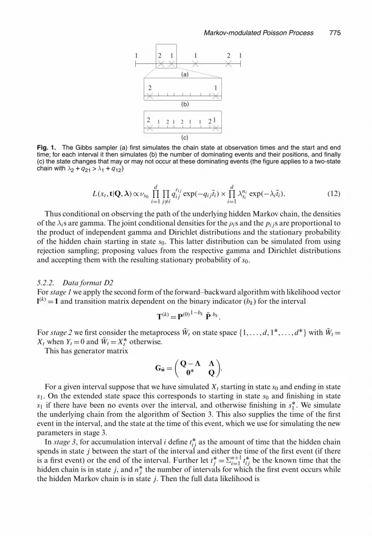
Fig. 1 shows the first two stages for data format D1.Stage 3 is especially simple using our conjugate priors. The likelihood for the full data (ob-

served data and path of the hidden chain) is


2 1 1 2

2 1

12 1 2 1 2 1 1 2

1 1

(a)

(b)

(c)

Fig. 1. The Gibbs sampler (a) first simulates the chain state at observation times and the start and endtime; for each interval it then simulates (b) the number of dominating events and their positions, and finally(c) the state changes that may or may not occur at these dominating events (the figure applies to a two-statechain with λ2 Cq21 >λ1 Cq12)

L.xt , t|Q, λ/∝νs0

d∏i=1

∏j �=i

qrij

ij exp.−qij t̃i/×d∏

i=1λni

siexp.−λit̃i/: .12/

Thus conditional on observing the path of the underlying hidden Markov chain, the densitiesof the λis are gamma. The joint conditional densities for the ρis and the pijs are proportional tothe product of independent gamma and Dirichlet distributions and the stationary probabilityof the hidden chain starting in state s0. This latter distribution can be simulated from usingrejection sampling; proposing values from the respective gamma and Dirichlet distributionsand accepting them with the resulting stationary probability of s0.

5.2.2. Data format D2For stage 1 we apply the second form of the forward–backward algorithm with likelihood vectorl.k/ =1 and transition matrix dependent on the binary indicator (bk) for the interval

T.k/ =P.0/1−bk P̄ bk :

For stage 2 we first consider the metaprocess W̄t on state space {1, . . . , d, 1Å, . . . , dÅ} with W̄t =Xt when Yt =0 and W̄t =XÅ

t otherwise.This has generator matrix

Gw̄ =(

Q−Λ Λ0Å Q

):

For a given interval suppose that we have simulated Xt starting in state s0 and ending in states1. On the extended state space this corresponds to starting in state s0 and finishing in states1 if there have been no events over the interval, and otherwise finishing in sÅ1 . We simulatethe underlying chain from the algorithm of Section 3. This also supplies the time of the firstevent in the interval, and the state at the time of this event, which we use for simulating the newparameters in stage 3.

In stage 3, for accumulation interval i define tÅij as the amount of time that the hidden chainspends in state j between the start of the interval and either the time of the first event (if thereis a first event) or the end of the interval. Further let tÅj =Σn+1

i=1 tÅij be the known time that thehidden chain is in state j, and nÅ

j the number of intervals for which the first event occurs whilethe hidden Markov chain is in state j. Then the full data likelihood is


L.xt , t|Q, λ/∝νs0

d∏i=1

∏j �=i

qrij

ij exp.−qij t̃i/×g∏

j=1λ

nÅj

j exp.−λjtÅj /: .13/

We then proceed as with data format D1.

5.2.3. Data format D3For data format D3 we consider the metaprocess Vt on extended state space {1.0/, . . . , d.0/,1.1/, . . . d.1/, . . . , 1.cmax/, . . . , d.cmax/, 1Å} as defined in Section 4.1.2.

For the application of the forward–backward algorithm in stage 1, the transition matricesare T.k/ =P.ck/ and the likelihood vectors are l.k/ =1. For stage 2, in simulating from the exactdistribution of the underlying chain for an interval where the start state is s0, the end state is s1and ck events are observed we use the generator matrix Gv as defined in equation (11) with startstate s0 but end state s

.ck/1 .

The algorithm also simulates from the exact distribution of the times at which each of theck events occurs over the interval; therefore we may perform stage 3 exactly as for data formatD1.

6. Analysis of Chi site data for Escherichia coli

6.1. Background and the Escherichia coli dataIn recent years there has been an explosion in the amount of data describing both the genomesof different organisms and the biological processes that affect the evolution of these genomes.There is much current interest in understanding the function of different features of the genomeand what affects the biological processes such as mutation and recombination. One approachto learning about these is via genome segmentation (e.g. Li et al. (2002)): partitioning a genomeinto regions that are homogeneous in terms of some characteristic (e.g. GC base pair content),and then looking for correlations between this characteristic and either another characteristicor a biological process of interest.

Here we consider segmentation of a bacterial genome based on the rate of occurrence of a par-ticular DNA motif—called the Chi site. The Chi site is a motif of eight base pairs: GCTGGTGG.The Chi site is of interest because it stimulates DNA repair by homologous recombination(Gruss and Michel, 2001), so the occurrence of Chi sites has been conjectured to be related torecombination hot spots.

Our data are for E. coli DNA and consist of the position (in bases) of Chi sites along thegenome. Fig. 2 shows a schematic diagram of the circular double-stranded DNA genome ofE. coli, with the two strands represented by the inner and outer rings. There is a 1–1 mapping ofbases between the outer and inner strands (C ↔ G and A ↔ T) so that each uniquely determinesthe other. Fig. 2 also indicates a directionality that is associated with different halves of eachstrand as split by the replication origin (O) and terminus (T). The molecular mechanisms ofDNA replication differ between the two half-strands and they are termed leading and lagging,as indicated in Fig. 2.

The 1–1 mapping between base pairs together with the reversing of directionality betweeninner and outer strands implies that searching the Chi site in the outer strand is equivalent tosearching for CCACCAGC in the inner strand. This sequence is sufficiently different from thesequence of the Chi site in the inner strand that occurrences of the Chi site in inner and outerstrands are effectively independent. The occurrences of Chi sites in leading and lagging halvesare also independent since these are separate parts of the genome. Thus our data consist of four


OT

Fig. 2. Schematic diagram of the leading ( ) and lagging (– – –) strands on the inner and outer ringsof the E. coli genome split by the replication origin (O) and terminus (T), together with the direction that isrelevant for Chi site identification

independent sets of positions of Chi sites—along leading and lagging halves of both inner andouter strands. Fig. 3 shows the cumulative number of events along the genome for each of thesedata sets.

The replication and repair mechanisms for leading strands are different from those for laggingstrands so in general we might expect them to have different compositional properties (densi-ties of nucleotides and oligonucleotides). A bias in the frequency of Chi sites favouring leadingstrands has been noted in several genomes, including E. coli (e.g. Karoui et al. (1999)), andis evident from Fig. 3. A more open question is whether there is variation within the leadingand/or lagging strands, rather than just between the leading and lagging strands.

Our aim is first to determine whether Chi sites appear to occur uniformly at random withineach of the leading and lagging strands, or whether there is evidence of the intensity of the occur-rence of Chi sites varying across either strand. Secondly, if there is variation then we would liketo infer the regions with strong evidence for either a high or low intensity of Chi sites.

The E. coli genome (defined as a single strand length) is 4639675 bases long so each of theindividual halves is 2319.838 kilobases long.

6.2. Model and priorWe analyse the positions of occurrences of the Chi site along first leading then lagging strandsby using our Gibbs sampler. These positions are discrete bases and our Gibbs sampler appliesto continuous data; however, each of the four strands is over 2319 kilobases long and containsfewer than 400 occurrences of the eight-base Chi site, so it is reasonable to model this discreteprocess as continuous. Furthermore, a straightforward approach to discrete modelling wouldinvolve applying the forward–backward algorithm across the entire genome, which would becomputationally prohibitive.

One of our aims is to perform model choice, and the choice of model will depend on thepriors for each model; in particular we cannot use uninformative priors (e.g. Bernardo andSmith (1995), chapter 6). For the results that we present here we take exponential priors (i.e.gamma densities with shape parameters equal to 1) for the λis and the ρis (gamma densitieswith shape parameter of less than 1 will lead to posteriors with an infinite density at 0), anduniform priors for the vectors of transition probabilities.


0 500 1000 1500 2000

300

200

100

0

kB

Cum

ulat

ive

# po

ints

Fig. 3. Cumulative number of occurrences of the Chi site along the genome for leading (C) and lagging (4)halves of the outer strand and leading (�) and lagging (r) halves of the inner strand

We first analyse the inner leading and lagging strands and use the results from these to informpriors for analyses of the outer leading and lagging strands, which we use to perform modelchoice. We also tested robustness of our results to variation in the priors.

We analyse the inner strands by using exponential priors, the means of which are chosenempirically from the data for each strand. The mean for all λ-parameters is set to n=tobs, wheren and tobs are respectively the number of Chi sites and the total length in kilobases of the strand.


The mean for all q parameters needs to be somewhere between 1=tobs and n=tobs for an analy-sis to be feasible, so we set it to

√n=tobs. These choices are rather arbitrary, but the resulting

posteriors are only used to inform the (weak) priors for the analyses of the outer strands.Since the priors for the inner strand are exchangeable and the likelihood of an MMPP is

invariant under permutation of the states, so also is the joint posterior. We therefore order theresults from the analysis of the inner strand such that λ1 �λ2 and use the posterior means asmeans for the exponential priors for the analysis of the outer strands. Since the runs for the outerstrands have non-exchangeable priors, we may not order the output and must treat it exactly asit appears.

For each strand we analyse the one-dimensional case analytically and the two-dimensionaland three-dimensional cases using 100000 iterations of our Gibbs sampler. The Gibbs samplercode was written in C and, when run on an AMD Athlon 1458 MHz computer, took approx-imately 11 min to perform 100000 iterations on the outer lagging strand. This strand contains117 Chi sites.

Matrix exponentials were calculated by truncating equation (4). The truncation was set sothat the error in each element of the matrix exponential was less than a predetermined tolerance(this was efficient as errors decay faster than geometrically, and accurate as it involves summingonly positive values). The sum can be evaluated efficiently for all interval lengths by calculatingand storing the required powers of M once for each iteration. The powers of M are also thenused when simulating the underlying hidden chain.

6.3. ResultsFig. 4 shows trace plots for the first 20000 iterations and autocorrelation functions over thefirst 10000 iterations for the two-dimensional run on the lagging strand of the outer ring. Thetrace plot for λ1 shows one of only six mode-switch-and-returns (all brief), indicating thatthe different priors fix quite firmly the ordering of the states. These brief switches, however,exert a strong (and spurious for our purposes) influence on the autocorrelation functions, andso we show autocorrelation functions for a period in which there is no mode switching; themixing appears to be satisfactory.

Posterior model probabilities for the leading and lagging strands were calculated by using themethod of Chib (1995) and are given Table 1. They indicate a clear choice of a two-dimensionalmodel over a one-dimensional model for the lagging strand. There is also substantial evidencefor a two-dimensional model in preference to a three-dimensional model. From the model prob-abilities alone there is nothing to choose between one-, two- and three-dimensional models forleading strands.

For the two-dimensional model for lagging strands the posterior mean parameter values

Table 1. Posterior model probabilities for leading and lagginghalves of the outer strand

Data set Probabilities for the following models:

One Two Threedimensional dimensional dimensional

Lagging (outer) < 0:01 0.83 0.17Leading (outer) 0.30 0.44 0.26


0 5000 10000 15000 20000

02.051.0

01.050.0

00.0

iteration0 5000 10000 15000 20000

iteration

1adbmal

0.1−

5.1−

0.2−

5.2−

0.3−

5.3−

0.4−

) 21q(0 1gol

0 10 20 30 40

0.18.0

6.04.0

2.00.0

Lag0 10 20 30 40

Lag

FC

A

0.18.0

6.04 .0

2.00.0

FC

A

Fig. 4. Trace plots for the first 20000 iterations and autocorrelation functions for the first 10000 iterationsof the Gibbs sampler for the lagging strand of the outer ring with non-exchangeable priors derived from therun for the lagging strand of the inner ring


correspond to intensities of 20.8 and 92.1 Chi sites per megabase, and an intensity of 16.0transfers per megabase from the lower state to the higher state and 21.1 transfers per megabasefrom the higher state to the lower state. The one-dimensional model for leading strands has aposterior mean intensity of 164.7 Chi sites per megabase.

Posterior model probabilities may be sensitive to the exact prior that is used and, since thedata contain less information about the q-parameters than the λ-parameters, the q-priors maybe particularly influential. We performed further analyses of the outer and inner rings withexchangeable exponential priors for λ and with exchangeable exponential, (approximately) nor-mal and truncated exponential priors for q. There was little change in the posterior means forordered .λ1, λ2/, but a large amount of variability in .q12, q21/ as expected. However, the pos-terior model probabilities always indicated at least a two-state model for lagging strands andlittle to choose between one- and two-state models for leading strands.

A possible biological explanation for our results is given by how replication differs on leadingand lagging strands. Leading DNA strands are replicated continuously whereas lagging strandsare replicated in fragments. It may be the fragmentary nature of replication that is causing theheterogeneity in the rate of occurrence of Chi sites.

We can use the output of the Gibbs sampler to perform segmentation of the lagging strandson the basis of the intensity of the occurrence of Chi sites. Fig. 5 plots the mean (over 1000chains sampled every 100 iterations) intensity against position along the genome. This gives a‘smoothed signal’ of Chi site intensity which could be used to evaluate correlations with (say)recombination rates across the genome. An alternative segmentation might be based on theposterior probabilities that a given point along the genome is in each of the possible states—forthis segementation, at each point the chain is simply set to the state with the highest posteriorprobability.

7. Discussion

We have presented a novel approach to simulating directly from the conditional distributionof a continuous time Markov process and shown how this can be used to implement a Gibbssampler for analysing MMPPs. The Gibbs sampler can analyse data where the event times aredirectly observed, and also data where the number of events or even only the presence or absenceof events is known for a sequence of time intervals.

The Gibbs sampler has some advantages over standard Metropolis–Hastings samplers. Firstly,the Gibbs sampler requires no tuning; tuning for Metropolis–Hastings algorithms can be timeconsuming—especially for long data sets where the algorithm takes longer to run and foralgorithms involving blocking of parameters. Further such tuning is valid for the area of theposterior being explored while the tuning takes place (hopefully the mode); there is no guaranteethat it will be appropriate for yet unseen tail areas that the algorithm should eventually explore.

Secondly, a by-product of the Gibbs sampler is that we can investigate the posterior distri-bution of the underlying chain. This allowed us to identify regions of high intensity of Chi siteoccurrences on the lagging strand of E. coli DNA.

There has been previous work on developing a Gibbs sampler for MMPPs. Scott (1999) andScott and Smyth (2003) have presented an approximate Gibbs sampler that can be applied tocertain MMPPs, assuming that the event times are directly observed. Their approximation is toassume that certain state changes coincide precisely with observed events. In many situationsthis approximation will be negligible; Scott (1999) modelled times at which a bank account isaccessed, where a criminal may or may not have obtained the bank details; it is argued that itis sensible to define the arrival of a criminal as the time at which he or she first accesses the


0 500 1000 1500 2000

21.001.0

80.060.0

40.020.0

00.0

distance along chain

ytisnetni naem

Fig. 5. Mean λ-value from 1000 chains at each point in the lagging strand

account. Further Scott and Smyth (2003) argued that forcing state changes to start and end atevent times ‘eliminates the possibility of pathological bursts containing no events’. However,their Gibbs sampler also places restrictions on the allowable state changes: all transitions tostates with lower intensities than the current state are permitted but, out of all the (ordered)states with higher intensity than the current state, transitions are only permitted to the statethat is immediately adjacent to the current state. Also the approximation of restricting state


changes to event times will become less accurate as the rates of the generator for the hiddenchain increase towards the same order of magnitude as the intensities of the observed process.Our Gibbs sampler avoids these issues and there is little extra cost in implementing it.

Blackwell (2003) and Bladt and Sørensen (2005) used rejection sampling to sample from theexact distribution of a discretely observed continuous time Markov process. A chain is simu-lated forward from a given observed state, and if the simulated state at the next observationtime does not match the corresponding observed state then the chain is rejected and the processis repeated until a match is achieved. A similar technique could replace stage 2 of our Gibbssampler, where we simulate from the hidden chain and the observed event process and acceptthe hidden chain if the chain finishes in the correct state and there are no observed events. Thisis efficient only when the number of rejected chains is small. It is straightforward to calculatethe expected number of simulations until acceptance for an interval of known length given thestart and end states. We calculated this for the simulated states at event times at every iterationof our Gibbs sampler for every one of the 1164 intervals in a data set that was simulated overan observation window of 100 s with intensities λ1 = 10 and λ2 = 13 and rates for the hiddenMarkov chain q12 = q21 = 1. On average for about 700 of the intervals three or fewer chainsimulations were expected to be required. However, the distribution of the expected numberof simulations had a very heavy right-hand tail, with about 200 intervals requiring at least 10simulations and about 20 requiring more than 100 simulations, so the mean expected numberof simulations per interval was around 20. This number is likely to increase as the number ofhidden states increases. In practice stage 2 of our Gibbs sampler takes a very small proportionof the central processor unit time and this would be likely to remain small if rejection samplingwere to be used instead, unless the number of rejections was large.

We considered the application of MMPPs to modelling the occurrence of a specific DNAmotif in E. coli. We found evidence for heterogeneity in the occurrence of this DNA motif, theChi site, in the lagging strand; this may have a biological explanation in terms of the replicationprocess on this strand. The output of our Gibbs sampler also enables us to segment the laggingstrand into regions of high and low intensity of these Chi sites. Ideally we would like to use thissegmentation to test for correlation of high Chi site intensity with regions of high recombinationrates, but unfortunately data are not currently available on the variation in recombination ratein E. coli.

A computer program, which was written in C, which implements the Gibbs sampler forevent time data is available from http://www.maths.lancs.ac.uk/∼sherlocc/MMPP/index.html.

Acknowledgements

We dedicate this paper to the memory of Nick Smith who helped with the application of ourmethod to the analysis of E. coli DNA. The first author acknowledges support from Engineeringand Physical Sciences Research Council grants GR/R91724/01 and GR/T19698/01.

References

Asmussen, S. (2000) Matrix-analytic models and their analysis. Scand. J. Statist., 27, 193–226.Baum, L. E., Petrie, T., Soules, G. and Weiss, N. (1970) A maximisation technique occurring in the statistical

analysis of probabilistic functions of Markov chains. Ann. Math. Statist., 41, 164–171.Bernardo, J. M. and Smith, A. F. M. (1995) Bayesian Theory. Chichester: Wiley.Blackwell, P. G. (2003) Bayesian inference for Markov processes with diffusion and discrete components. Biomet-

rika, 90, 613–627.


Bladt, M. and Sørensen, M. (2005) Statistical inference for discretely observed Markov jump processes. J. R.Statist. Soc. B, 67, 395–410.

Burzykowski, T., Szubiakowski, J. and Ryden, T. (2003) Analysis of photon count data from single-moleculefluorescence experiments. Chem. Phys., 288, 291–307.

Chib, S. (1995) Marginal likelihood from the Gibbs output. J. Am. Statist. Ass., 90, 1313–1321.Davison, A. C. and Ramesh, N. I. (1996) Some models for discretised series of events. J. Am. Statist. Ass., 91,

601–609.Fearnhead, P. and Meligkotsidou, L. (2004) Exact filtering for partially observed continuous time models. J. R.

Statist. Soc. B, 66, 771–789.Fischer, W. and Meier-Hellstern, K. (1992) The Markov-modulated Poisson process (MMPP) cookbook.

Perform. Evaln, 18, 149–171.Gilks, W. R., Richardson, S. and Spiegelhalter, D. J. (eds) (1996) Markov Chain Monte Carlo in Practice. London:

Chapman and Hall.Gruss, A. and Michel, B. (2001) The replication-recombination connection: insights from genomics. Curr. Opin.

Microbiol., 4, 595–601.Karoui, M. E., Biaudet, V., Schbath, S. and Gruss, A. (1999) Characteristics of chi distribution on different

bacterial genomes. Res. Microbiol., 150, 579–587.Kou, S. C., Xie, X. S. and Liu, J. S. (2005) Bayesian analysis of single-molecule experimental data (with discussion).

Appl. Statist., 54, 469–506.Li, W., Bernaola-Galvan, P., Haghighi, F. and Grosse, I. (2002) Applications of recursive segmentation to the

analysis of DNA sequences. Comput. Chem., 26, 491–510.Ross, S. (1996) Stochastic Processes, 2nd edn. York: Wiley.Ryden, T. (1996) An EM algorithm for estimation in Markov-modulated Poisson processes. Computnl Statist.,

21, 431–447.Scott, S. L. (1999) Bayesian analysis of a two-state Markov modulated Poisson process. J. Computnl Graph.

Statist., 8, 662–670.Scott, S. L. and Smyth, P. (2003) The Markov modulated Poisson process and Markov Poisson cascade with

applications to web traffic modelling. Bayes. Statist., 7, 1–10.Sherlock, C. (2005) Discussion on ‘Bayesian analysis of single-molecule experimental data’ (by S. C. Kou, X. S.

Xie and J. S. Liu). Appl. Statist., 54, 500–501.

Documents

An exact Gibbs sampler for the Markov-modulated Poisson process