eScholarship provides open access, scholarly publishingservices to the University of California and delivers a dynamicresearch platform to scholars worldwide.

Department of Economics, UCSBUC Santa Barbara

Title:An Experiment on Nash Implementation

Author:Charness, Gary B, University of California, Santa BarbaraCabrales, Antonio, Universidad Carlos III de MadridCorchon, Luis C

Publication Date:06-13-2001

Series:Departmental Working Papers

Permalink:http://escholarship.org/uc/item/8275577k

Keywords:Implementation, Experiments, Mechanisms.

Abstract:We perform an experimental test of a modification of the controversial canonical mechanism forNash implementation, using 3 subjects in non-repeated groups, as well as 3 outcomes, states ofnature, and integer choices. We find that this mechanism successfully implements the desiredoutcome a large majority of the time, providing empirical evidence for the feasibility of suchimplementation. In addition, the performance is further improved by imposing a fine on a dissident,so that the mechanism implements strict Nash equilibria. While our environment is stylized, ourresults offer hope that experiments can identify reasonable features for practical implementationmechanisms.

Copyright Information:All rights reserved unless otherwise indicated. Contact the author or original publisher for anynecessary permissions. eScholarship is not the copyright owner for deposited works. Learn moreat http://www.escholarship.org/help_copyright.html#reuse

An Experiment on Nash Implementation*

Antonio Cabrales, Gary Charness, and Luis C. Corchón‡

June 13, 2001

Abstract: We perform an experimental test of a modification of the controversial

canonical mechanism for Nash implementation, using 3 subjects in non-repeated groups,

as well as 3 outcomes, states of nature, and integer choices. We find that this mechanism

successfully implements the desired outcome a large majority of the time, providing

empirical evidence for the feasibility of such implementation. In addition, the

performance is further improved by imposing a fine on a dissident, so that the mechanism

implements strict Nash equilibria. While our environment is stylized, our results offer

hope that experiments can identify reasonable features for practical implementation

mechanisms.

Key Words: Implementation, Experiments, Mechanisms.

JEL classification: C72, C91, C92, D70, D78.

* We would like to thank James Costain, Esther Hauk, Rosemarie Nagel, Diego Rodriguez, Joel Sobel, and seminar participants at University of Bern, Universitat de Girona, the Universidad Pública de Navarra, Universidad del País Vasco, Universitat Pompeu Fabra, the October 1998 ESA meeting, and the ESEM99 for helpful comments. The financial support of Spain's Ministry of Education under grants PB98-0024, BEC2000-1029, and Generalitat de Catalunya under grant 1997SGR-00138 is gratefully acknowledged. ‡ Contact: Cabrales, Universitat Pompeu Fabra: Ramon Trias Fargas 25-27, E-08005 Barcelona, Spain; Corchón, Universidad Carlos III: Madrid 126, E-28903 Getafe, Spain. Charness (corresponding author), Universitat Pompeu Fabra: Ramon Trias Fargas 25-27, E-08005 Barcelona, Spain; charness@upf.es

1. INTRODUCTION

The theory of implementation addresses the problem of designing mechanisms

whose equilibria satisfy certain socially desirable properties, but which do not require

that the authorities have unrealistically accurate information about the underlying

parameters of the economy. Mechanism design is important in many social choice

problems, such as the selection of candidates for an election, the design of a constitution,

or the optimal allocation of resources in economies with public goods. Several

theoretical mechanisms have been discussed in the literature and some have been studied

experimentally.1 Yet these mechanisms either work only for a limited set of

environments or do not seem to fare well empirically.

In this paper, we perform an experimental test of a modification of the canonical

mechanism for implementation in Nash equilibria (see Maskin 1999, and Repullo 1987),

and provide some encouraging empirical evidence regarding the feasibility of this

mechanism. This mechanism is important because it allows the implementation in Nash

equilibria in any possible environment of any Nash implementable social objective.

We require the agents to announce the state of the world (the hidden information

in which the planner is interested), an outcome (for example, an allocation of private and

public goods and perhaps side payments) and an integer. If everyone announces the same

state, or if there is only one departure from a consensus announcement, the integer is not

1 Chen and Tang (1998) conduct a comparative study of the basic quadratic mechanism of Groves and Ledyard (1977) and the Paired-Difference Mechanism by Walker (1981). Elbittar and Kagel (1997) compare the performance of Moore's (1992) and Perry and Reny's (1999) mechanisms to implement the efficient allocation of an indivisible private good among two players (King Solomon's dilemma). Sefton and Yavas (1996) study the mechanism proposed by Abreu and Matsushima (1992). Katok, Sefton & Yavas (2001) compare the Abreu and Matsushima mechanism (1992) with the Glazer and Perry (1996) mechanism, finding that the predicted outcome is rarely observed in either case.

1

relevant in determining the outcome. If there is more than one such departure from

unanimity, the person who announces the highest number gets her announced outcome.

It is easy to prove that such a game cannot have an equilibrium where, with

positive probability, there is more than one deviation; the artful part of the design is to

permit and require the right kind of consensus to be the equilibrium. Our experiment

models an environment where there are three states of the world (preference profiles) and

three outcomes. The preferences of the three agents cycle around these three outcomes in

the three states, but the social choice rule picks a specific one in each state of the world.

We concentrate on such a rule for several reasons: First, we show that it is not

implementable in dominant strategies, so that it is natural to look for a mechanism that

implements in Nash equilibria. Second, there is no focal choice in each state, and some

agent does sufficiently poorly (in comparative terms) in the allocation prescribed by the

social choice rule that, unless there is an enforcing mechanism, telling the truth is not an

obvious choice. At the same time the environment is simple enough to be understood by

the subjects. While our environment is quite stylized, we make successful

implementation as difficult as possible by assigning conflicting preferences to each of

three types. Since the problem is therefore non-trivial, successful performance would

offer hope that this mechanism could be effective in more general environments.

We conducted 4 sessions, 2 in each of two treatments. The first treatment (the

baseline) uses the mechanism as described. In the 2nd treatment we introduce a fine if

and only if there is a dissident,2 so that the mechanism implements strict Nash equilibria.

The likelihood of the desired outcome being implemented was .68 in the baseline

treatment and .80 in the 2nd treatment. Both proportions represent a substantial degree of

2

implementation, particularly with respect to the obvious comparison to an uninformed

planner. As the introduction of fines enhances the observed effectiveness, this suggests

that there is room for improvement to the modified canonical mechanism.

Yet implementation of the desired outcome often occurs as a consequence of

people playing strategy profiles which are not Nash equilibria in pure strategies.3 We

offer an ad hoc, but plausible, explanation of this fact based on two elements: (1) a taste

for truth-telling - agents prefer to tell the truth (ceteris paribus), and so are willing to

accept some (possibly small) monetary losses in return for doing so; and (2) risk

aversion. If the preferences with respect to telling the truth can be described by an extra

“monetary equivalent” amount inserted in the utility function, then the subject

preferences can be totally described by two parameters, the monetary equivalent to the

truth and the coefficient of relative risk aversion.4

While we do not claim to have fully resolved this puzzle, and are aware that our

environment is not general, we feel that the clear patterns we observe and the relative

success of this mechanism offer hope for identifying reasonable features for practical

implementation mechanisms.

2. THE SOCIAL CHOICE PROBLEM

The canonical mechanism for implementation in Nash equilibria can implement a

wide variety of social choice rules, under a large domain of preferences. Yet this

2 This term is defined in section 2.1. 3 This was the case for 55 of the 68 successful implementations in the baseline treatment and for 60 of the 80 successful implementations by the mechanism with fines. 4 We suppose that subjects have utility functions with constant relative risk aversion, so that their preferences with respect to risk can be described by a single parameter.

3

mechanism is quite controversial: According to Jackson (1992), “A nagging criticism of

the theory is that the mechanisms used in the general constructive proofs have ‘unnatural’

features.” Moore (1992) also asserts that the mechanisms for Nash implementation are

“highly complex - often employing some unconvincing device such as an integer game.”

If this argument holds, one might expect rather limited success for Nash implementation.

Under these circumstances, an experimental test may offer some insight.

This version of the mechanism requires a truly infinite strategy space (i.e.,

allowing all integers). We modify the mechanism because this requirement seems

incompatible with an experiment having a finite duration. Our design uses a common

modification of the mechanism in which players can choose from a finite number (3 in

our case) of integers. If these integers are needed to determine the outcome, they are

added together; on the basis of this sum (modulo 3), one player’s announced outcome is

selected. With this modification, the mechanism implements the social choice rule in

pure-strategy Nash equilibrium, that is, the only pure-strategy Nash equilibrium outcome

for each state corresponds to the outcome of the social choice rule.5

We describe our mechanism formally in section 2.1 and offer a motivation in

section 2.2.

2.1 The environment and the mechanism

Let us first describe the environment in which the mechanism is to be used. There

are three individuals indexed by i ∈{1,2,3} , three possible outcomes (a, b, c), as well as

three states of the world (red, yellow, green). The preferences of the individuals among

the outcomes in the three states of the world can be described by:

4

TABLE 1: PREFERENCES

State

Red Yellow Green

Player 1 a f b f c b f c f a c f a f b

Player 2 b f c f a c f a f b a f b f c

Player 3 c f a f b a f b f c b f c f a

With these preferences any deterministic single-valued social choice function

must, in every state, assign the worst outcome in the preference ordering to one of the

players. This will be seen to have important implications for the properties of the

mechanisms that implement such social choice functions.

We now introduce the social choice function that we wish to implement with our

experimental design:

F(red) = a F(yellow) = c F(green) = b

Proposition 1: The social choice function F(•) cannot be implemented in

dominant strategies.

Proof: See Appendix A.

This result makes apparent the necessity of implementing with a different

equilibrium concept. The obvious choice in this case is to implement in Nash

5 However, there are mixed strategy equilibria that have different outcomes with positive probability.

5

equilibrium. We will use a version of the canonical mechanism for Nash implementation

(Maskin 1999, Repullo 1987, McKelvey 1989). Let us now describe the mechanism.

Strategy space:

Let Θ = {red, yellow, green} be the set of states. Let Λ = {a, b, c}, and N = {1, 2, 3}.

The individual strategies belong to Θ × Λ× N.

Outcome function:

1. If the 3 individuals announce:

red, the outcome is F(red) = a,

yellow, the outcome is F(yellow) = c,

green, the outcome is F(green) = b.

2. If exactly two agents announce red and:

1 announces yellow, the outcome is b,

1 announces green, the outcome is c,

otherwise the outcome is a.

3. If exactly two agents announce yellow and:

2 announces red, the outcome is b,

2 announces green, the outcome is a,

otherwise the outcome is c.

4. If exactly two agents announce green and:

3 announces red, the outcome is c,

3 announces yellow, the outcome is a,

otherwise the outcome is b.

5. If the three agents announce different states, then the integers announced by

the three players are added.

6

If the sum is 4 or 7, then the outcome is the one chosen by player 1.

If the sum is 5 or 8, then the outcome is the one chosen by player 2.

If the sum is 3, 6 or 9 then the outcome is the one chosen by player 3.

Proposition 2: This mechanism implements F(•) in pure-strategy Nash equilibrium.

Proof: See Appendix A.

Note that there are also mixed-strategy equilibria which produce outcomes

different from the ones in F(•). These equilibria may be useful for understanding the

experimental results. The standard canonical mechanism6 implements in pure and mixed

strategy Nash equilibria. The difference with the mechanism used here is that in the

classical version the players can announce any integer, and the outcome is the one

announced by the person who announces the highest integer (ties can be broken

arbitrarily). As mentioned above, this modification is dictated by practical concerns.

Another important issue is that the pure strategy equilibria of the mechanism are

such that some players are using a weak best response. The reason is that the outcome

these agents receive in equilibrium is the least-preferred one for them. Thus, there would

be no harm in changing the strategy used, if the other players continue using the

equilibrium strategies. This, however, does not imply that the equilibrium strategy (which

involves announcing the true state) is weakly dominated for the player who gets the least

preferred outcome under F(•). It can be checked (from the Table that summarizes

payoffs in the instructions) that there are some combinations of strategies for the other

6 As described by Repullo, for example.

7

players such that announcing the true state results in the most preferred outcome. Even

taking this into account, it will be clear from the experimental results that the incentive to

deviate from the equilibrium is quite important.

However, there are some weakly dominated strategies. If an agent does not

announce her most preferred outcome under the true state of the world, she is using a

strategy that is weakly dominated (by another that announces the same state and integer

and the most preferred outcome). This will serve us as an indirect check of whether the

agents understood the workings of the mechanism.

To check the importance of the fact that equilibrium strategies are weak best

responses for some agents, we created a version of the mechanism which modifies rules 2

- 4 and punishes a solo deviation by any agent for whom deviating is a weak best

response. Any such deviating agent we call a dissident. In this way the mechanism

implements in strict Nash equilibria (recall that strict equilibria must be in pure

strategies). Cabrales (1999) shows that when implementation is in strict Nash equilibria,

boundedly rational agents are able to reach the equilibrium and will stay there. This need

not happen when agents have multiple best responses at equilibrium. This argument

suggests that the performance of the modified game may lead to better results. The

complete rules for the new mechanism can be found in Appendix C; here we describe the

revised rule:

1. If exactly two agents announce red and:

1 announces yellow, the outcome is b,

1 announces green, the outcome is c,

8

otherwise the outcome is a and the dissident pays a fine of x pesetas.7

As we will see in the data section, this change does make a difference in the

behavior of the players and the proportion of times that the outcome F(•) is attained. The

following corollary is straightforward from Proposition 2.

Corollary 2: The modified mechanism implements F(•) in strict Nash

equilibrium.

2.2 Motivation

We motivate the social choice problem and the mechanism used to solve it with

problems from constitutional design and from optimal allocation of resources. This

presentation highlights the fact that the mechanism we use can potentially be applied to a

wide array of problems.

Constitutional design: A country called Freedonia was founded two hundred

years ago. The founding fathers designed a constitution establishing the rules of the

game and the civil rights to which the citizens of Freedonia are entitled. The rules that

are of immediate interest to us are as follows. The constitution distinguishes three

possible states:

• Foreign threat (denoted by red in the formal description below), which occurs

when it is likely that an enemy country attacks Freedonia.

7 The fine in our design was either 100 or 200 pesetas (depending on the circumstances), or between 10%

9

• Home threat (denoted by green in the formal description below), which occurs

when there are riots that cannot be controlled by normal police force.

• Normality (denoted by yellow in the formal description below), which occurs

when the rest of the constitution applies.

Three actions can be taken:

• General Mobilization (denoted by a)

• Suspension of certain civil rights (denoted by b)

• No particular action (denoted by c).

The founders could not predict when each of these contingencies would occur,

nor the preferences for the person in each role in each state. But they devised the rules

(the mechanism) through which the legitimate powers of Freedonia could decree which

of the actions should be taken. These rules are:

1. There are three people who can give an opinion about the state in which

Freedonia finds itself: the president of Freedonia (representing the executive

power), the speaker of the Parliament (representing the legislative power) and

the most senior member of the Supreme Court (representing the judiciary).

2. At the beginning of each parliamentary session, each of these individuals

sends a message to the High Notary of the Republic. The messages, sent

simultaneously and without consultation, declare the state in which the

and 20% of expected payoffs in a round. See the instructions for details.

10

Republic finds itself (red, yellow, green), the action to be taken (a, b, c), and

an integer (1, 2, 3)

3. The rules that determine the action finally taken are described in section 2.1

under the label “Outcome function”, where agent 1 is the president, agent 2 is

the speaker and agent 3 the supreme court member.

The aim of this procedure was to achieve, for each state, the actions specified by

the social choice function in section 2.1. The founders thought this would work, having

anticipated that preferences for these three agents (described in section 2.1 under

“Preferences”) would be such that the only pure strategy Nash equilibrium of the game in

each state yields the desired outcome (see Proposition 2).

Optimal resource allocation: Suppose that a government has two possible sectors

in which to spend money: police and environment. There are two possible levels of

expenditure (H and L); budget constraints make it impossible to spend H in both sectors.

Thus, there are only three alternatives: (a) spend H on police and L on environment, (b)

spend L on police and H on environment, and (c) spend L on both police and

environment. There are three players (groups of voters), each representing a different

“region”.

The “states” describe the three possible profiles of preference orderings of the

economic alternatives identified in Table 1. In addition, the preferences of player 1 are

the more “intense” ones in state red, the preferences of player 2 are the more intense ones

in state yellow, and the preferences of player 3 are the more intense ones in state green.

A player with intense preferences is more likely to organize a violent revolt if her first

11

preference is not implemented, and the planner’s objective is to keep the social peace. So

the planner prefers (a) in state red, (c) in state yellow, and (b) in state green.

3. EXPERIMENTAL DESIGN

Sessions were conducted at the Universitat Pompeu Fabra in Barcelona. There

were 15 participants in each session. The average net pay was about $10 per subject and

sessions lasted less than 2 hours.8

Achieving comprehension and salience in this experiment was non-trivial. At the

beginning of a session, the instructions and a decision sheet were passed out to each

subject. The decision sheet stated the subject number and type. Instructions covered all

rules used to determine the outcome for each group and the resulting payoffs to each

player in the group; these were read aloud to the entire room. As the experimental set-up

is not a familiar environment, the instructions also contained an example where the states

of Nature were types of weather, the outcomes were activities, and the 3 types had

different state-dependent preferences among these activities.9 The complete instructions

can be found in Appendix C.

To aid comprehension, we included complete payoff tables and seven exercise

questions, which were discussed aloud. When the instructional phase was concluded, we

proceeded with the session. As there were 5 subjects of each type, we had 5 groups of

three in each of the 10 rounds of the experiment.10 These groups were varied - an

8 The pay might seem low by U.S. standards; however, students have very low opportunity costs. This is demonstrated by the ease of recruiting for experiments at Pompeu Fabra. 9 We thank James Costain for this idea. 10 As we conducted our sessions by hand (perhaps thereby increasing the credibility of the random draw), it was not feasible to have more than 10 periods in a session.

12

anonymous matching process was devised so that no two groups ever had the same

composition.11 This non-repeat feature was public knowledge.

At the start of a round, a monitor made a blind draw (with replacement) of a

colored card from a box held by the experimenter. This box contained 3 yellow, 4 green,

and 5 red cards.12 The color drawn was the state of Nature and was known to all. On

their decision sheets, participants then announced a color, an integer from {1,2,3}, and a

preferred outcome. As described in section 2.2, if all three members of a group

announced different colors, the sum of the integers chosen determined which member's

preferred outcome was implemented. Since each type was aware of the true state of

Nature, each type has a unique preference among the possible outcomes. Thus, we have

one rationality test embedded in the experiment - if a subject did not choose her preferred

outcome, it would appear that the instructions were not well understood.

The decision sheets were collected, announcements collated, and outcomes and

payoffs determined. An individual's payoff for the period was written on her decision

sheet (see Appendix C) and the sheets were returned to the subjects. The next round was

then initiated by another draw from the box of colored cards. Subjects were made aware

that the experiment would continue until 10 rounds were completed. At the end of the

session, participants were paid based on the payoffs achieved in a randomly-selected

round.13

11 With 15 players in groups of three, and 10 periods, it is not mathematically possible to arrange matters so that no two players are ever in the same group twice. 12 This deliberate asymmetry was an attempt to create a bit of friction, perhaps making successful implementation somewhat more difficult. 13 This was done in an attempt to make payoffs more “salient” to the subjects, as this method makes the nominal payoffs 10 times as large as would be the case if payoffs were aggregated over 10 periods.

13

As mentioned earlier, two types of sessions were conducted. The baseline session

featured payoffs of 500, 1000, or 1500 pesetas, with 500 pesetas added as a show-up fee.

In the 2nd treatment, where we explore whether the disincentive of a fine would enhance

the mechanism's success rate, a fine of 100 or 200 pesetas (depending on the combination

of type and the state of Nature; see the instructions) was deducted from a dissident's

payoff. This modification cannot guarantee that it is the dissident who is being dishonest,

but it does make false reporting riskier.

At the end of the session, each participant was paid individually and privately.

We did not employ the two-stage lottery payoff procedure (e.g., Roth and Malouf 1979),

as many observers (e.g., Selten et al. 1999) feel that this is not very effective in

experiments, and we also felt that there was already sufficient complexity in our

experimental design.14

4. RESULTS

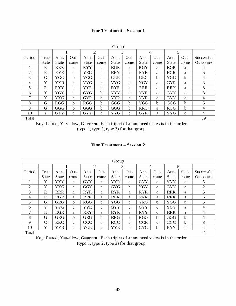
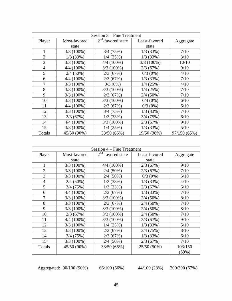
Detailed data for all sessions are shown in Appendix D. The success of the

mechanism in implementing F(•) is considerable. We find that the social choice function

was successfully implemented in 68 of 100 instances in the baseline treatment - 35 of 50

in session 1, and 33 of 50 in session 2. This rate increased to 80% in the treatment with a

fine for a dissident - 39 of 50 in session 3 and 41 of 50 in session 4. Figure 1 shows the

rate of successful implementation by periods for each treatment; there is no clear trend

across time.

14 It is also worth noting that, according to the theory no correction for risk preferences should be needed, as the equilibrium would be in pure strategies and the outcome would not be random.

14

FIGURE 1

Rate of Successful Implementation over Time

0%

20%

40%

60%

80%

100%

1 2 3 4 5 6 7 8 9 10Period

BaselineFine

We can make a statistical comparison between the observed success rate in the

baseline treatment and the success rate if a planner simply implements policy based on

the most likely state (here red, with p = 512

). On this basis, the rate of successful

implementation would have been no more than 60% in any of the 4 sessions.15 While the

test of the equality of proportions16 rejects the hypothesis of identical success rates at a

significance level of p < .001, this test treats each individual observation as being

independent. We can perform a more conservative test by ranking the rates of successful

15 The number of (red, green, yellow) draws in sessions 1-4 were (3,4,3), (6,2,2), (3,3,4), and (3,3,4). Even if the planner were told ex ante which state would be the most common and implemented for this state, success rates would always be lower than ours. 16 See Glasnapp and Poggio (1985). The specific test statistic is Z =

RB − RF

SPC

, where Ri is the rate of

successful implementation in treatment i, and the estimate of the standard error of (RB − RF ) is:

SPC=

RB − RF

(RC )(1−RC )( 1N B

+ 1N F

), where RC =

RBNB + RF NF

NB + NF

is the estimate of the population proportion

under the null hypothesis of equal proportions, and Ni is the number of observations in treatment i.

15

implementation in our sessions to the rate of successful implementation for an

uninformed planner, assuming the most likely state (either ex ante or ex post) has

occurred. The nonparametric Wilcoxon-Mann-Whitney rank-sum test (see Siegel and

Castellan 1988) ranks these eight rates (4 sessions x 2 implementation methods), and

shows that we obtain significantly more (p = .014) successful implementation.

We also find that the fine increases the success rate significantly from that

observed in the baseline mechanism (and obviously also in comparison to the rate in the

simulated sessions). By ranking the rates of successful implementation for each true state

in each session, we obtain 6 observations in each treatment (2 sessions*3 states), or 12

observations in all. Once again, the Wilcoxon test indicates a significant difference (p =

.013) in the rates of successful implementation.17 This rank-sum test can also be used to

compare individual truth-telling rates for the 30 subjects in each treatment, yielding a

significant difference (p = .004) for a comparison across the two treatments.18

We find that the proportion of subjects who announce the true state follows a

consistent pattern: The likelihood that a subject makes a true announcement is directly

related to the payoff the subject would receive if all group members reported the state

truthfully. This pattern is reassuring and provides further evidence that the subjects

17 While the outcomes in each state are not truly independent (since the same subjects makes choices in different true states), their circumstances are different. Cooper and Kagel (2000) present evidence suggesting that there is generally little transfer across games and roles in experiments. 18 As we do not have convergence in our limited number of periods, there is some concern that this difference across treatments may be sensitive to results in individual periods. However, even if we exclude from our analysis that period (10) with the greatest difference across treatments, the results of the Wilcoxon test on successful outcomes across treatments (by state of nature) remain significant at p = .047. The test results on individual truth-telling across treatments are still significant at p = .011; overall, excluding this 10th period reduces the difference in the rates of successful implementation across treatments only from 80% vs. 68% to 80% vs. 71%.

16

understood the payoffs in the game. Table 2 shows the likelihood of a true

announcement in each state for each treatment:19

TABLE 2 – AGGREGATED TRUTHFUL REPORTING

Treatment Most-favored state 2nd-favored

state

Least-favored state Total

Baseline

93/100 (93%)

55/100 (55%)

23/100 (23%)

171/300 (57%)

Fine

90/100 (90%)

66/100 (66%)

44/100 (44%)

200/300 (67%)

The overall rate of truth-telling is 57% in the baseline treatment, and 67% in the

2nd treatment. Notice that the biggest behavioral change, where the associated rate of

truthful announcements nearly doubles, is observed for the type who would receive the

lowest payoff if all types told the truth. The patterns are largely confirmed on the

individual level: The rate of truth-telling in these 3 cases is similarly (weakly)

monotonically decreasing for 40 of the 60 participants. Appendix C presents detail on

truthful reporting by individual and state. Figures 2 and 3 show how the individual truth-

telling rates depend on the favorability of the state in our treatments:

19 The agents have been re-labeled, so that the types here correspond to the ranking of the outcome of the social choice function in a state.

17

FIGURE 2

Individual Frequency of Truth-telling – Baseline Treatment

0

0.2

0.4

0.6

0.8

1

.00 .17 .25 .33 .50 .67 .75 .83 1.00Truthful Reporting Rate

Best state2nd stateWorst state

FIGURE 3

Individual Frequency of Truth-telling – Fine Treatment

0

0.2

0.4

0.6

0.8

1

.00 .17 .25 .33 .50 .67 .75 .83 1.00Truthful Reporting Rate

Best state2nd stateWorst state

18

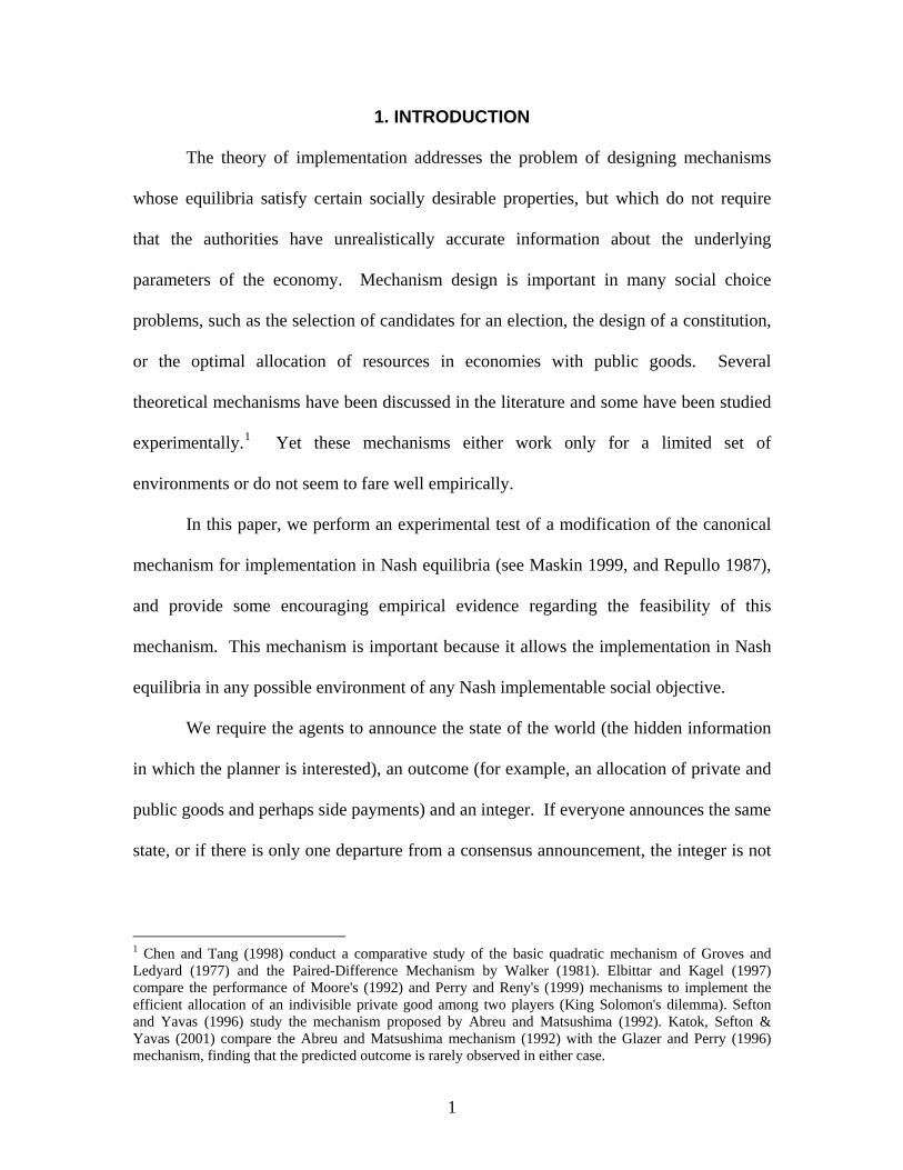
In both treatments, around four-fifths of the subjects reported the true state

whenever it was the most favorable one, with similar patterns across treatments for the

remaining minority. For the 2nd state, truth-telling in the baseline treatment is first-order

stochastically dominated by truth-telling in the fine treatment. However, it is visually

clear that the biggest difference on an individual level is seen in behavior when the least

favorable state is drawn. The dramatic difference in truth-telling rates across roles is

evidence that people did not simply report the true state because it was focal, but rather

were (at least to a substantial degree) able to understand the instructions and make

reasoned choices.

We also note that the observed sample variance for the number of successful

implementations in each treatment is much lower with a fine: 0.67 (fine) vs. 2.40

(baseline); there appears to be less uncertainty in this environment. This inference is also

supported by the observation that the integer game was needed to determine the outcome

18% of the time in the baseline case, but with a likelihood of only 7% when a fine was

possible. This difference in rates is significant at p < .02, by the equality of proportions

test.

Finally, the implicit comprehension test provided by the announced preferred

outcomes indicates a reasonable level of general understanding, as 34 of the 60 subjects

selected the appropriate outcome in all 10 rounds and, on average, 84% of all announced

outcomes were individually optimal. Figure 4 shows the distribution of “comprehension

scores.”

19

FIGURE 4

Comprehension Scores: % of Time Choosing Correct Outcome

0%

20%

40%

60%

80%

100%

0 1 2 3 4 5 6 7 8 9 10Number of Corrrectly Chosen Outcomes

5. DISCUSSION

Two patterns are clear from the data. The first is that the mechanism achieves

substantial success in terms of obtaining the outcome that F(•) selects, despite the

conflicting preferences of the three agents in a group. The second is that the observed

behavior conforms more with the pure-strategy Nash equilibrium when the fines are

introduced.

In any pure-strategy Nash equilibrium profile, all players tell the truth. We do not

observe this, as the observed frequency of the Nash equilibrium profile is around 0.13 in

the baseline treatment, and around 0.20 in the treatment with fines. To obtain the

outcome desired by the social choice function it is sufficient that the first player and

20

either the second or third announce the truth. This explains a major portion of the success

of the mechanism in implementing F(•).20

To explain the players' behavior leading to these results, we concentrate on the

game without fines.21 To make the analysis simpler, we will focus on the case where the

true state is red; the game is the same (subject to re-labeling) for yellow or green. We

now summarize the information of the observed behavior from Table 2, aggregating the

results after relabeling the games for the 3 states so that they represent the same game:

TABLE 3: FREQUENCY OF ANNOUNCED OUTCOMES

State

Red Yellow Green

Player 1

93

5

2

Player 2

23

27

50

Player 3

54

40

6

When the true state is red, the player 1 agent gets her favorite outcome under F(•),

player 3 gets her middle outcome, and player 2 gets her worst outcome. It turns out that,

given the actual strategies of the other players, announcing red is indeed a best response

for player 1, for most specifications of the risk preferences. For this reason we neglect

the uncertainty in the behavior of player 1, simply assuming she always tells the truth.

20 Note that given the observed frequencies, the probability that the most favored player plus at least one of the others announce the truth is 0.93*(.54 + .23 - .54*.23) ≅ 0.60 in the baseline, compared to 0.68 correct implementation. In the fine treatment, we have 0.90*(.66 + .45 - .66*.45) ≅ 0.73, compared to the correct implementation rate of 0.80.

21

The behavior of the player 2 and player 3 is a little more difficult to explain.

Consider the game that results for player 2 and 3 once the strategy of player 1 is fixed as

red. To simplify even further, assume that the three integers are used about one third of

the time and that players always announce their most favorite outcome in the true state of

the world (these assumptions are in line with observed behavior). Let

Eu(I) =u(5)+ u(10)+ u(15)

3. The game between players 2 and 3 is then as follows:

TABLE 4: PAYOFFS FOR REDUCED GAME

Player 3 choice

Red Yellow Green

Red

u(5), u(10)

u(5), u(10)

u(5), u(10)

Yellow

u(5), u(10)

u(10), u(15)

Eu(I), Eu(I)

Player 2

choice

Green

u(5), u(10)

Eu(I), Eu(I)

u(15), u(5)

Strategy green is weakly dominated for player 3, and given that strategies yellow

and green are used a significant proportion of the time by player 2, it is not (absent other

considerations) a best response for 3 to use green. This readily explains the low observed

frequency of this strategy for player 3. We now propose some plausible explanations for

the remaining behavior.

One surprising observation, given Table 4, is that player 2 uses strategy red a

significant proportion of the time despite its being weakly dominated (independently of

21 The explanations given here also work well for the game with fines, as shown in Appendix B.

22

risk preferences). Learning or bounded rationality cannot explain this fact. Even under a

learning hypothesis, a strategy that is used in the limit must be at least almost as good (in

the limit) as the alternatives. First, notice that player 3 rarely chooses green. So strategy

red for player 2 would be as profitable as yellow or green in the limit, if the proportion of

the time that player 3 uses yellow becomes very small over time. But an examination of

the data in Appendix D shows that this is not the case (for example, when the true state

was red in one of the last three periods of the baseline treatment, 6 out of 15 times player

3 reported yellow). If the players are confused and not reasoning very well, they should

make other types of “mistakes” more often, like playing yellow or green when they are

player 1, or playing green when they are player 3.

A plausible alternative explanation is that using strategy red gives some of the

subjects that play as player 2 some utility above the purely monetary return. Playing red

is “the truth”, so they may get utility from doing so. Since all types get their preferred

outcome in some states of the world, perhaps people feel that the outcome is fair if all

individuals tell the truth.

One must also explain the significant number of yellow and green choices by

player 2, and red and yellow by player 3. If the players were all risk neutral, yellow

would be weakly dominated for 2 and red would be weakly dominated for 3. As before,

learning or bounded rationality is not the most plausible explanation in this case. Some

taste for truth-telling might explain why some individuals choose red in the player 3 role.

But this cannot explain the choice of yellow by player 2. Since green is riskier than

yellow, a degree of risk aversion for some players could explain the observed choices.

23

In Appendix B we perform a small calibration exercise, which shows that neither

the taste for truth-telling nor the degree of risk aversion need be very large to justify the

actual choices made in the experiment. While these explanations for the observed

behavior are ad hoc, other stories do not seem suitable; thus we feel that our

interpretation is plausible. Furthermore, the behavior in the game with fines can also be

explained (even numerically, as shown in Appendix B) with the same arguments. In fact,

the calibration appears to be robust in the sense that the calibrated values for the two

models (with and without fines) are the same.

To summarize, the observed behavior can be explained with players that are very

mildly risk averse and have some preference for truth-telling. The first part of the

explanation is mainstream economics and seems quite plausible (even for the low stakes

involved in the experiment), as the degree of risk aversion necessary is really quite small.

While the second part may be more controversial, we have not found a better explanation.

Ascertaining whether subjects do actually have this preference would require an entirely

different design, and more theoretical efforts devoting to understanding the phenomenon.

Our experiment suggests that this might be a fruitful line of research.

6. CONCLUSION

We find that our canonical mechanism for Nash implementation can be quite

successful in implementing the social choice function, with an observed success rate of

68% in the baseline treatment. With the inclusion of a fine for being a dissident, the

mechanism's performance increases to 80%. Agents’ behavior may be explained by

taking into account some taste for truth-telling and possible risk preferences. Criticisms

24

that such a mechanism would prove too complex seem to be unfounded here, as

embedded comprehension tests offer evidence that most participants understood the

structure of the environment. A note of caution is advisable on this point, however: Our

environment has only 3 states; it is conceivable that the perceived complexity would

increase dramatically when the number of states increases. But as we argue below, the

increasing complexity may actually help, rather than harm, the rate of implementation.

From a theoretical standpoint, the results indicate that if social goals imply some

people will be treated badly (i.e., they get their least preferred allocation), these people

will depart from Nash equilibrium strategies. Therefore, failure to achieve the social goal

is not due to unnatural features of the mechanism, but perhaps is instead induced by

social goals being perceived as unfair.

An important question suggested by the experimental results is whether the

success rate in implementation can be sustained in a different environment, with more

agents, states and outcomes, and different utilities. This is especially pressing because the

success was obtained in spite of low Nash equilibrium frequencies. While the success rate

we observe may not be general, the tendencies we have seen in the data allow us to make

some conjectures about when the mechanism would be effective.

A major reason why the mechanism succeeds is that only two agents must play

the Nash strategies to obtain the Nash outcome. In general games, n −1agents need play

the Nash strategy to obtain the Nash outcome. While this would seem to make successful

implementation more difficult in general, note that to obtain anything different from the

integer game in the Nash mechanism a coincidence of n −1players is required anyway.

If, due to risk aversion, agents try to avoid the integer game (and the social choice

25

function does not treat them too unfavorably), announcing the truth seems like a clear

alternative. This could induce a reasonable success rate, which would be increased by a

taste for truth-telling in the population.

More empirical research is needed to settle the question. We hope that our study

encourages further experiments designed to develop practical implementation

mechanisms.

26

REFERENCES

Abreu, D. and H. Matsushima (1992), “Virtual Implementation in Iteratively Undominated Strategies: Complete Information,” Econometrica, 60, 993-1008. Barsky, R., F. Juster, M. Kimball, and M. Shapiro (1997), “Preference Parameters and Behavioral Heterogeneity: An Experimental Approach in the Health and Retirement Study,” Quarterly Journal of Economics, 112, 537-579. Cabrales, A (1999), “Adaptive Dynamics and the Implementation Problem with Complete Information,” Journal of Economic Theory, 86, 159-184. Chen, Y. and F. Tang, (1998) “Learning and Incentive Compatible Mechanisms for Public Goods Provision: An Experimental Study,” Journal of Political Economy, 106, 633-662. Chou, R., R. Engle, and A. Kane (1992), “Measuring Risk Aversion from Excess Returns on a Stock Index,” Journal of Econometrics, 52, 201-224. Cooper, D. and J. Kagel (2000), “Learning and Transfer in Signalling Games,” mimeo. Elbittar, A. and J. Kagel (1997), “King Solomon's Dilemma: An Experimental Study on Implementation,” mimeo. Glasnapp, D. and J. Poggio (1985), Essentials of Statistical Analysis for the Behavioral Sciences, Merrill: Columbus, OH. Glazer, J. and R. Rosenthal (1992), “A Note on Abreu-Matsushima Mechanisms,” Econometrica, 60, 1435-1438. Groves, T. and J. Ledyard (1977), “Optimal Allocation of Public Goods: a Solution to the Free Rider Problem,” Econometrica, 45, 783-809. Isaac, R. and J. Walker (1988), “Group Size Effects in Public Goods Provision: The Voluntary Contributions Mechanism,” Quarterly Journal of Economics, 103, 179-199. Jackson, M. (1992), “Implementation in Undominated Strategies: A Look at Bounded Mechanisms,” Review of Economic Studies, 59,757-775. Katok, E., M. Sefton & A. Yavas (2001), “Implementation by Iterative Dominance and Backward Induction: An Experimental Comparison,” mimeo, forthcoming in Journal of Economic Theory.

27

Maskin, E. (1977), “Nash Implementation and Welfare Optimality,” Review of Economic Studies, 66, 23-38. McKelvey, R. (1989), “Game Forms for Nash Implementation of General Social Choice Correspondences,” Social Choice and Welfare, 6, 139-156. Moore, J. (1992), “Implementation in Environments with Complete Information,” in J. Laffont, ed., Advances in Economic Theory: Sixth World Congress, Econometric Society. Perry, M. and P. Reny (1999), “A General Solution to King Solomon's Dilemma,” Games and Economic Behavior, 26, 279-285. Repullo, R. (1987), “A Simple Proof of Maskin's Theorem on Nash Implementation,” Social Choice and Welfare, 4, 39-41. Roth, A. and M. Malouf (1979), “Game-Theoretic Models and the Role of Bargaining,” Psychological Review, 86, 574-594. Sefton, M. and A. Yavas (1996), “Abreu-Matsushima Mechanisms: Experimental Evidence,” Games and Economic Behavior, 16, 280-302. Selten, R., A. Sadrieh, and K. Abbink (1999), “Money Does Not Induce Risk Neutral Behavior, But Binary Lotteries Do Even Worse,” Theory and Decision, 46, 211-49. Siegel, S. and N. Castellan (1988), Nonparametric Statistics for the Behavioral Sciences, McGraw-Hill: New York. Walker, M. (1981), “A Simple Incentive Compatible Scheme for Attaining Lindahl Allocations, Econometrica, 49, 65-71.

28

APPENDIX A: PROOFS OF PROPOSITIONS

Proposition 1: The social choice function F(•) cannot be implemented in dominant strategies.

Proof: By contradiction. To implement F(•) in dominant strategies there must a strategy

set S, an outcome function g : S → {a, b,c}, and strategies sij , such that si

j is dominant for

agent i in state ∈{1,2,3} j ∈{r, y,g}, where r stands for red, y for yellow, and g for green.

Since g(•) implements F(•) we must have that g(s1r ,s2

r ,s3r ) = a . Since a is the least

favorite outcome for player 2 under state r, and s2r is dominant for 2 under r, we must

have that g(s1r ,s2

y,s3r )= a . Similarly, since c is the least favorite outcome for player 3

under state y, and s is dominant for 3 under y, we must have that g3y (s1

y, s2y, s3

g ) = c . Also,

since b is the least favorite outcome for player 1 under state g, and s1g is dominant for 1

under g, we must have that g(s1r ,s2

g ,s3g ) = b.

Let mean “is weakly preferred to”. Now since s> 1r is dominant for 1 under r and

is dominant under y we must have that s1y

g(s1r ,s2

y,s3g ) > g(s1

y,s2y,s3

g ) for player 1 under

state r and g(s1y, s2

y, s3g ) > g(s1

r ,s2y,s3

g ) for player 1 under state y. Since we just showed that

g(s1y, s2

y, s3g ) = c , this implies that g(s1

r ,s2y,s3

g ) ≠ b.

Since s is dominant for 2 under y and s2y

2g is dominant under g we must have that

g(s1r ,s2

y,s3g ) > g(s1

r ,s2g,s3

g )for player 2 under state y and g(s1r ,s2

g ,s3g ) > g(s1

r , s2y,s3

g )for player

2 under state g. Since we just showed that g(s1r ,s2

g ,s3g ) = b, this implies that

g(s1r ,s2

y,s3g ) ≠ a.

Since s3r is dominant for 3 under r and s3

g is dominant under g we must have that

g(s1r ,s2

y,s3g ) > g(s1

r ,s2y,s3

r )for player 3 under state g and g(s1r ,s2

y,s3r ) > g(s1

r ,s2y ,s3

g )for player

3 under state r. Since we just showed that g(s1r ,s2

y,s3r )= a , this implies that

g(s1r ,s2

y,s3g ) ≠ c .

Since g(s1r ,s2

y,s3g ) ≠ b , g(s1

r ,s2y,s3

g ) ≠ a, and g(s1r ,s2

y,s3g ) ≠ c , and there are no other

outcomes we reach a contradiction and the result follows.

29

This result is useful to know because it makes apparent the necessity of

implementing with a different equilibrium concept. The obvious choice in this case is to

implement in Nash equilibrium.

Proposition 2: The mechanism described in the main text implements F(•) in pure strategy Nash equilibrium. Proof: First, notice that a strategy profile in which all agents announce the true state is a

Nash equilibrium, as the only agent who can change the outcome in that case is the one

who already has her favorite outcome.

Now we show that outcomes that are not desired by the social choice function

cannot be the outcome of a pure strategy equilibrium. For this we consider several

subcases:

1. Suppose that all agents are announcing untruthfully the same state. In this case there is an agent (agent 1 if the consensus is r, agent 2 if it is y, and 3 if it is g) that can change the outcome and strictly improve by announcing the true state.

2. Suppose that exactly 2 agents are announcing the same state. One of those agents is not getting her favorite outcome. That agent can change her announcement of the state in such a way that three different states will be announced. She can also choose the integer so that the outcome she announces is selected. If she chooses her favorite outcome she will obtain a strict improvement.

3. Suppose that the outcome is determined by looking at the integers. Then, either of the agents that is not obtaining her favorite outcome can change her announcement of the integer so that the outcome she announces is the one selected. If she also announces her favorite outcome she obtains a strict improvement.

Since this exhausts all cases, the results follows.

30

APPENDIX B: CALIBRATION OF RISK AVERSION AND “TASTE FOR TRUTH-TELLING” PARAMETERS

Let us first consider player 2. She uses strategy yellow and strategy green a significant proportion of the time. Suppose she believed that the probabilities for player 3 to use strategies (red,yellow,green) are respectively (0.54, 0.40, 0.06) as we observe in the data. Assume also that her preferences exhibit constant relative risk aversion,22 so that u(c) =

cα

α (for α ≤1,α ≠ 0 ). Under this assumption the value of α that is necessary

to make a player 2 indifferent between yellow and green is 0.20. The usual estimated values for this parameter23 are between -1 and –4, which represent even higher aversion to risk; however, the estimates are obtained for decisions that involve much higher stakes than the ones in our experiment. The literal interpretation is that the choices come from individuals that are indifferent between green and yellow and randomize between them in the observed proportions. The alternative interpretation (the “purification” approach to mixed strategies, see Harsanyi) is that preferences are heterogenous, so that some players (27/77 to be precise) are more risk averse than α = 0.20 and choose yellow, and some others (50/77) are less risk averse than α = 0.20 and choose green.24 In any case, it seems that a reasonably small degree of risk aversion by at least some subjects can explain the fact that player 2 uses strategies yellow and green. It is more difficult to make sense of the significant use of strategy red by player 2. In the game depicted in Table 4, we can see it is a weakly dominated strategy. Now assume that players get some utility out of telling the truth, so that the utility of red for player 2 is not u but rather u(5) (5+ k). Under this assumption, and for the value of α = 0.20, a player with a value of k = 1.93 would be indifferent between red, yellow, and green. If we use the same parameters (α = 0.20, k = 1.93) with agent 3, the ratio of the expected utilities of strategies red and yellow (assuming the probabilities for the strategies of 2 are the observed frequencies in our data) is 1.02, which is not a bad approximation for indifference.25 While α may not differ between players, k could depend on the strategic situation facing the agent. For player 3 there is some “external” enforcement of truth telling, since by not telling the truth she risks getting 5 instead of 10.26 The value of k that makes player 3 indifferent between red and yellow is k = 0.79.

22 We realize that this is a strong assumption, but the parameter is only intended to capture the attitudes toward risk for the small range of values that pertain to the experiment. 23 See Barsky et al. (1997) or Chou, Engle and Kane (1992) and references therein. 24 The problem with the second interpretation is that, if the players’ beliefs are constant over time, each individual would choose the same strategy all the time. But the last Table in Appendix D shows that individual subjects did change strategy choices during the experiment. It could be that their beliefs changed with experience, and sometimes their best response was one strategy and sometimes it was the other. 25 Given that in our case u(0) has been normalized to 0, the ratio of utilities is invariant to the utility representation for any two Von Neumann-Morgenstern utility functions. 26 It might be that this reduces the “cognitive dissonance”associated with lying (see Akerlof 1982).

31

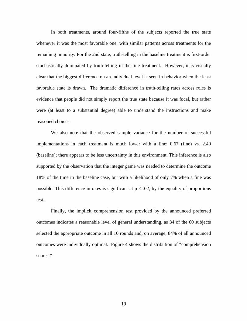
Now let us examine the game when there are fines. After the appropriate re-labeling, the observed frequencies of play are shown in Table 5:

TABLE 5: NUMBER OF TIMES EACH STRATEGY IS PLAYED

State

Red Yellow Green

Player 1

90

10

0

Player 2

45

30

25

Player 3

66

30

4

If we again fix the behavior of player 1 as a truthful announcement, the resulting game for players 2 and 3 is:

Player 3 choice

Red Yellow Green

Red

u(5), u(10)

u(5), u(8)

u(5), u(8)

Yellow

u(4), u(10)

u(10), u(15)

Eu(I), Eu(I)

Player 2

choice

Green

u(4), u(10)

Eu(I), Eu(I)

u(15), u(5)

Again, we first consider player 2. If she also believed that the probabilities for player 3 are the observed frequencies in the data, and using α = 0.20 as in the baseline treatment, the ratio of the utilities of yellow and green is 1.00058. If we used the value of k = 0.79 that makes player 3 indifferent between red and yellow in the baseline treatment, the ratio of expected utilities of strategies red and yellow for player 2 in the fine treatment is 1.00853. As for player 3, the ratio of utilities between strategies red and yellow using α = 0.20 and k = 0.79 is 1.013. Thus, we find that there are values of k and α that explain most of the deviation from the pure strategy Nash equilibrium in both games.

32

APPENDIX C: INSTRUCTIONS

Most instructions are identical for both treatments. Differences are indicated.

Thank you for participating in this experiment. In this experiment, there are 10 periods and 3 types of people. The result of those periods will determine the money that you will receive in this experiment. We have given you a sheet of paper with spaces to do an announcement in every period. Your identification number and your type are printed on them and will not change during the experiment. In each period, you will be in a group with two other people, so that every group has one person of each type. The other people in your group will not be constant for all ten periods; instead, participants will be re-matched, by identification numbers, with others for each period. While you may be matched with the same person(s) on more than one occasion, you will not know it and at no point will you ever know the identification # or the identity of the other group members in any period.

Your benefits in each period are determined by the combination of the “state of nature” (a color drawn randomly), your “preferences” in that state of nature, and one of 3 possible “outcomes” that will be decreed by a central processor in each period using the information provided. The state of nature (red, yellow or green) is obtained randomly at the beginning of the period and is revealed to all the participants. The 3 different types of people have different preferences among the outcomes in each state of nature and consequently different benefits in every case. Each period you will make an announcement about the state of nature in that period. You can announce any color you wish (it does not have to be the color that was drawn). Your announcement changes neither your preferences nor the state of nature, but it is part of the information used by the central processor to determine the outcome. The state of nature is the color of a card drawn randomly from a box in which there are 3 yellow cards, 4 green cards, and 5 red cards. The card drawn is shown publicly to everyone in the room. An announcement includes a color, an outcome, and an integer from {1, 2, 3}. The central processor will use the integers and the announced outcome to determine the decreed outcome when each of the 3 group members announces a different color. Although these terms are intended to be quite general, here is a specific example:

Consider the state of nature to be the “weather”, the announcement to be a “weather report” and the outcome to be an “activity”. Suppose the weather may be either “hot” (red), “warm” (yellow), or “cold” (green), and that there are 3 possible activities: exercising (a), watching TV (b), and reading (c). Think of the 3 types as three different siblings and the central processor as an absent tutor, who must decide on an activity for her children for the day without knowing the weather, using only the children’s weather reports. If the weather is hot (red):

A type 1 prefers exercise (a), next prefers TV (b), and least prefers reading (c).

33

A type 2 prefers TV (b), next prefers reading (c), and least prefers exercise (a). A type 3 prefers reading (c), next prefers exercise (a), and least prefers TV (b).

If the weather is warm (yellow): A type 1 prefers TV (b), next prefers reading (c), and least prefers exercise (a).

A type 2prefers reading (c), next prefers exercise (a), and least prefers TV (b). A type 3 prefers exercise (a), next prefers TV (b), and least prefers reading (c).

If the weather is cold (green):

A type 1 prefers reading (c), next prefers exercise (a), and least prefers TV (b). A type 2 prefers exercise (a), next prefers TV (b), and least prefers reading (c). A type 3 prefers TV (b), next prefers reading (c), and least prefers exercise (a).

The following table summarizes this information:

red yellow green 1 a > b > c b > c > a c > a > b 2 b > c > a c > a > b a > b > c 3 c > a > b a > b > c b > c > a

MONETARY BENEFITS IN PESETAS FOR THE CHOSEN PERIOD

We assume that there is a monetary equivalent for the utility enjoyed by the activities. The 9 statements below describe the money received by the three types of players in each state of nature: In state red, a type 1 receives 1500 with outcome a, 1000 with outcome b ,and 500 with outcome c. a type 2 receives 500 with outcome a, 1500 with outcome b, and 1000 with outcome c. a type 3 receives 1000 with outcome a, 500 with outcome b, and 1500 with outcome c. In state yellow: a type 1 receives 500 with outcome a, 1500 with outcome b ,and 1000 with outcome c. a type 2 receives 1000 with outcome a, 500 with outcome b, and 1500 with outcome c. a type 3 receives 1500 with outcome a, 1000 with outcome b, and 500 with outcome c. In state green: a type 1 receives 1000 with outcome a, 500 with outcome b ,and 1500 with outcome c. a type 2 receives 1500 with outcome a, 1000 with outcome b, and 500 with outcome c.

34

a type 3 receives 500 with outcome a, 1500 with outcome b, and 1000 with outcome c. [In treatment 2, the payoffs described above are modified in some cases, as described in points 2, 3, and 4 of the OUTCOME RULES for treatment 2]

OUTCOME RULES • If the 3 group members announce:

red, then the outcome is a yellow, then the outcome is c green, then the outcome is b

We can summarize this information in the following way:

RRR = a, YYY = c, GGG = b

The first capital letter denotes the announcement of type 1 (R stands for red, Y for yellow and G for green), the second capital letter is the announcement of type 2, the third capital letter is the announcement of type 3, and the lowercase letter after the equal sign denotes the outcome, given these announcements.

• If exactly two group members announce red, the outcome is a, unless the group

member announcing something different is a type 1. In that case if the type 1 announces yellow, the outcome is b; if the type 1 announces green, the outcome is c.

RRY = a, RRG = a, RYR = a, RGR = a, YRR = b, GRR = c

[In treatment 2 add: If the announcement is RRY or RRG, then the type 3 group member will receive 200 pesetas less than the amount shown in the payoff table for treatment 1. If the announcement is RYR or RGR, then the type 2 group member receives 100 pesetas less than the quantity shown in the payoff table for treatment 1.]

• If exactly two group members announce yellow, the outcome is c, unless the group member announcing something different is a type 2. In that case if the type 2 announces red, the outcome is b; if the type 2 announces green, the outcome is c.

YYR = c, YYG = c, RYY = c, GYY = c, YRY = b, YRY = a

[In treatment 2 add: If the announcement is RYY or GYY, then the type 1 group member will receive 200 pesetas less than the amount shown in the payoff table for treatment 1. If the announcement is YYR or YYG, then the type 3 group member receives 100 pesetas less than the quantity shown in the payoff table for treatment 1.]

35

• If exactly two group members announce green, the outcome is b, unless the group member announcing something different is a type 3. In that case if the type 3 announces red, the outcome is c; if the type 3 announces yellow, the outcome is a.

GYG = b, GRG = b, YGG = b, RGG = b, GGY = a, GGR = c

[In treatment 2 add: If the announcement is GYG or GRG, then the type 2 group member will receive 200 pesetas less than the amount shown in the payoff table for treatment 1. If the announcement is YGG or RGG, then the type 1 group member receives 100 pesetas less than the quantity shown in the payoff table for treatment 1.]

• If all 3 members of a group announce different colors, then the central processor adds

the three integers selected by the 3 group members. The processor in this case will decree the announced outcome ( a, b , or c) by one of the group members.

That group member is chosen in the following way:

If the sum is 4 or 7, then the group member is the type 1 person. If the sum is 5 or 8, then the group member is the type 2 person. If the sum is 3, 6,or 9, then the group member is the type 3 person.

RYG(3) = 3 RYG(4) = 1 RYG(5) = 2 RYG(6) = 3 RYG(7) = 1 RYG(8) = 2 RYG(9) = 3

The number in parenthesis to the right of the equal sign is the sum of the announced integers, and the number to the left of the equal sign is the type of the agent whose announced outcome will become the decreed outcome. The same thing that happens with YGR also happens with YRG, GYR, GRY, RYG, and RGY.

(Notice that there are as many combinations that sum to 4 or 7 - exactly 9 - as there are for 5 or 8, or even for 3, 6 or 9).

PROCEDURE

When the experiment begins, a color will be randomly drawn and you will write an announcement in your sheet. The announcement consist of declaring at the same time a state of the world (red, yellow or green), an integer in {1,2,3} and an outcome in {a,b,c}. The announcement sheets will then be collected and the announcements will be processed to determine the outcome, either a, b, or c. The experimenter will then compute your benefits for the period and your announcement sheet will be returned to you with these indicated. You will only be informed of your payoffs. You will not be informed of the announcements or payoffs of other group members. Next we will proceed to the following period. At the end of 10 periods, the experiment will end. Each person will receive a show-up fee and the benefits obtained in

36

the period selected to be the payment period. Each person will be paid individually and privately. The payment period will be chosen at random at the end of the experiment. We will have cards numbered from 1 to 10. A student will select one of these cards at random and the number of the card selected will determine the payment period.

EXERCISES

To ensure that people understand how the mechanism works, we will do some exercises.

1. Suppose that the monitor draws a red card and all group members announce red.

What is the outcome? What is the state of nature? What are the payoffs for the type 1 person? the type 2 person? the type 3 person?

1. Suppose that the monitor draws a red card and types 2 and 3 announce red, while

type 1 announces green. What is the outcome? What is the state of nature? What are the payoffs for the type 1 person? the type 2 person? the type 3 person?

2. Suppose that the monitor draws a green card and types 1 and 3 announce green,

while type 2 announces red. What is the outcome? What is the state of nature? What are the payoffs for the type 1 person? the type 2 person? the type 3 person?

3. Suppose that the monitor draws a green card and all group members announce

yellow? What is the outcome? What are the payoffs for the type 1 person? the type 2 person? the type 3 person?

4. Suppose that the monitor draws a green card and types 1 and 3 announce yellow,

while type 2 announces green. What is the outcome? What are the payoffs for the type 1 person? the type 2 person? the type 3 person?

6. Suppose the monitor draws a yellow card, types 1, 2, and 3 announce (respectively)

red, yellow, and green, the integers 1, 2, and 3, and the outcomes a, b, and c. What is the outcome? What are the payoffs for the type 1 person? the type 2 person? the type 3 person?

7. Suppose the monitor draws a yellow card, types 1, 2, and 3 announce (respectively)

red, yellow, and green, the integers 1, 2, and 2, and the outcomes c, b, and c. What is the outcome? What are the payoffs for the type 1 person? the type 2 person? the type 3 person?

Once the experiment begins, all communication between participants is strictly forbidden.

Please ask questions before we begin. Are there any questions?

37

[PAYOFF SUMMARY TABLE FOR TREATMENT 1]

The following tables may be of help in summarizing the information about payoffs.

True State

Announcements R Y G

RRR 1500, 500, 1000 500, 1000, 1500 1000, 1500, 500

RRY 1500, 500, 1000 500, 1000, 1500 1000, 1500, 500

RRG 1500, 500, 1000 500, 1000, 1500 1000, 1500, 500

RYR 1500, 500, 1000 500, 1000, 1500 1000, 1500, 500

RGR 1500, 500, 1000 500, 1000, 1500 1000, 1500, 500

YRR 1000, 1500, 500 1500, 500, 1000 500, 1000, 1500

GRR 500, 1000, 1500 1000, 1500, 500 1500, 500, 1000

YYY 500, 1000, 1500 1000, 1500, 500 1500, 500, 1000

YYR 500, 1000, 1500 1000, 1500, 500 1500, 500, 1000

YYG 500, 1000, 1500 1000, 1500, 500 1500, 500, 1000

GYY 500, 1000, 1500 1000, 1500, 500 1500, 500, 1000

RYY 500, 1000, 1500 1000, 1500, 500 1500, 500, 1000

YGY 1500, 500, 1000 500, 1000, 1500 1000, 1500, 500

YRY 1000, 1500, 500 1500, 500, 1000 500, 1000, 1500

GGG 1000, 1500, 500 1500, 500, 1000 500, 1000, 1500

YGG 1000, 1500, 500 1500, 500, 1000 500, 1000, 1500

RGG 1000, 1500, 500 1500, 500, 1000 500, 1000, 1500

GYG 1000, 1500, 500 1500, 500, 1000 500, 1000, 1500

GRG 1000, 1500, 500 1500, 500, 1000 500, 1000, 1500

GGY 1500, 500, 1000 500, 1000, 1500 1000, 1500, 500

GGR 500, 1000, 1500 1000, 1500, 500 1500, 500, 1000

38

[PAYOFF SUMMARY TABLE FOR TREATMENT 2]

The following tables may be of help in summarizing the information about payoffs.

True State

Announcements R Y G

RRR 1500, 500, 1000 500, 1000, 1500 1000, 1500, 500

RRY 1500, 500, 800 500, 1000, 1300 1000, 1500, 300

RRG 1500, 500, 800 500, 1000, 1300 1000, 1500, 300

RYR 1500, 400, 1000 500, 900, 1500 1000, 1400, 500

RGR 1500, 400, 1000 500, 900, 1500 1000, 1400, 500

YRR 1000, 1500, 500 1500, 500, 1000 500, 1000, 1500

GRR 500, 1000, 1500 1000, 1500, 500 1500, 500, 1000

YYY 500, 1000, 1500 1000, 1500, 500 1500, 500, 1000

YYR 500, 1000, 1400 1000, 1500, 400 1500, 500, 900

YYG 500, 1000, 1400 1000, 1500, 400 1500, 500, 900

GYY 300, 1000, 1500 800, 1500, 500 1300, 500, 1000

RYY 300, 1000, 1500 800, 1500, 500 1300, 500, 1000

YGY 1500, 500, 1000 500, 1000, 1500 1000, 1500, 500

YRY 1000, 1500, 500 1500, 500, 1000 500, 1000, 1500

GGG 1000, 1500, 500 1500, 500, 1000 500, 1000, 1500

YGG 900, 1500, 500 1400, 500, 1000 400, 1000, 1500

RGG 900, 1500, 500 1400, 500, 1000 400, 1000, 1500

GYG 1000, 1300, 500 1500, 300, 1000 500, 800, 1500

GRG 1000, 1300, 500 1500, 300, 1000 500, 800, 1500

GGY 1500, 500, 1000 500, 1000, 1500 1000, 1500, 500

GGR 500, 1000, 1500 1000, 1500, 500 1500, 500, 1000

39

Payments when the three group members announce different states [for both treatments]:

True State Sum of

integers

Selected type,

announced outcome R Y G

3 3, a 1500, 500, 1000 500, 1000, 1500 1000, 1500, 500

3 3, b 1000, 1500, 500 1500, 500, 1000 500, 1000, 1500

3 3, c 500, 1000, 1500 1000, 1500, 500 1500, 500, 1000

4 1, a 1500, 500, 1000 500, 1000, 1500 1000, 1500, 500

4 1, b 1000, 1500, 500 1500, 500, 1000 500, 1000, 1500

4 1, c 500, 1000, 1500 1000, 1500, 500 1500, 500, 1000

5 2, a 1500, 500, 1000 500, 1000, 1500 1000, 1500, 500

5 2, b 1000, 1500, 500 1500, 500, 1000 500, 1000, 1500

5 2, c 500, 1000, 1500 1000, 1500, 500 1500, 500, 1000

6 3, a 1500, 500, 1000 500, 1000, 1500 1000, 1500, 500

6 3, b 1000, 1500, 500 1500, 500, 1000 500, 1000, 1500

6 3, c 500, 1000, 1500 1000, 1500, 500 1500, 500, 1000

7 1, a 1500, 500, 1000 500, 1000, 1500 1000, 1500, 500

7 1, b 1000, 1500, 500 1500, 500, 1000 500, 1000, 1500

7 1, c 500, 1000, 1500 1000, 1500, 500 1500, 500, 1000

8 2, a 1500, 500, 1000 500, 1000, 1500 1000, 1500, 500

8 2, b 1000, 1500, 500 1500, 500, 1000 500, 1000, 1500

8 2, c 500, 1000, 1500 1000, 1500, 500 1500, 500, 1000

9 3, a 1500, 500, 1000 500, 1000, 1500 1000, 1500, 500

9 3, b 1000, 1500, 500 1500, 500, 1000 500, 1000, 1500

9 3, c 500, 1000, 1500 1000, 1500, 500 1500, 500, 1000

40

DECISION SHEET Player type: Identification number:

Period State of the world Integer Outcome Payoff

1

2

3

4

5

6

7

8

9

10

41

APPENDIX D: RESULTS

Baseline Treatment – Session 1

Group 1 2 3 4 5

Period True State

Ann.State

Out-come

Ann.State

Out-come

Ann.State

Out-come

Ann.State

Out-come

Ann.State

Out-come

Successful Outcomes

1 Y RYR a YRR b YYY c GYY c YYY c 3 2 Y YYG c RYG a YYY c YYR c RYG b 3 3 G GRR c GGG b GRG b YRG a YRG c 2 4 G GGG b GGG b YRR b YGG b YRG c 4 5 R RGY b RGR a RGG b RYR a GGY a 3 6 G GRR c RGG b RGG b YGG b YGG b 4 7 Y YYY c GYR b YYR c YYY c GYY c 4 8 R RYR a RYR a RYR a RGY b RGR a 4 9 G GGG b YGG b RGG b YGG b YGG b 5

10 R RGR a RYY c RGR a RYG c RGR a 3 Total 35

Key: R=red, Y=yellow, G=green. Each triplet of announced states is in the order (type 1, type 2, type 3) for that group

Baseline Treatment – Session 2

Group 1 2 3 4 5

Period True State

Ann.State

Out-come

Ann.State

Out-come

Ann.State

Out-come

Ann.State

Out-come

Ann.State

Out-come

Successful Outcomes

1 R RRG a RRR a RRR a RGR a RRR a 5 2 R RRY a RGY a YGY a RGY b RGR a 4 3 G YGG b GGG b GRG b RRG a YRG c 3 4 R RGR a RYR a RRY a RGY b RYY c 3 5 Y YYR c YYR c YYR c YYG c GGR c 5 6 R RGR a RYR a RGY a RYR a RYR a 5 7 R RGY b RYY c YYR c YYY a GYY a 2 8 G GRG b RRG a YRG a RRG a YGG b 2 9 Y GYG b RYR a YYR c YYR c YYG c 3

10 R RYY c RGY c RGY b RGR a RYY c 1 Total 33

Key: R=red, Y=yellow, G=green. Each triplet of announced states is in the order (type 1, type 2, type 3) for that group

42

Fine Treatment – Session 1

Group 1 2 3 4 5

Period True State

Ann.State

Out-come

Ann.State

Out-come

Ann.State

Out-come

Ann.State

Out-come

Ann.State

Out-come

Successful Outcomes

1 R RRR a RYY c RGR a RGY a RGR a 4 2 R RYR a YRG a RRY a RYR a RGR a 5 3 G YGG b YGG b GRR c GRG b YGG b 4 4 Y YYR c YYG c YYG c YGY a GYR a 3 5 R RYY c YYR c RYR a RRR a RRY a 3 6 Y YGY a GYG b YYY c YYR c GYY c 3 7 Y YYG c GYR b YYR c YYR c GYY c 4 8 G RGG b RGG b GGG b YGG b GGG b 5 9 G GGG b GGG b GGG b RRG a RGG b 4

10 Y GYY c GYY c YYG c GYR a YYG c 4 Total 39

Key: R=red, Y=yellow, G=green. Each triplet of announced states is in the order (type 1, type 2, type 3) for that group

Fine Treatment – Session 2

Group 1 2 3 4 5

Period True State

Ann.State

Out-come

Ann.State

Out-come

Ann.State

Out-come

Ann.State

Out-come

Ann.State

Out-come

Successful Outcomes

1 Y YYY c GYY c YYR c GYY c YYY c 5 2 Y YYG c GGY a GYG b YGY a GYY c 2 3 R RRR a RYR a RYR a RYR a RRR a 5 4 R RGR a RRR a RRR a RRR a RRR a 5 5 G GRG b RGG b YGG b YRG b YGG b 5 6 Y YYG c YYR c GYY c GYY c YGY a 4 7 R RGR a RRY a RYR a RYY c RRR a 4 8 G GRG b GRG b RRG a RGG b GGG b 4 9 G RRG a GGG b RGG b GGR c GGG b 3

10 Y YYR c YGR c YYR c GYG b RYY c 4 Total 41

Key: R=red, Y=yellow, G=green. Each triplet of announced states is in the order (type 1, type 2, type 3) for that group

43

TRUTH-TELLING BY INDIVIDUALS AND STATES

Session 1 – Baseline Treatment Player Most-favored

state 2nd-favored state Least-favored

state Aggregate

1 3/3 (100%) 2/3 (67%) 4/4 (100%) 9/10 2 3/3 (100%) 1/3 (33%) 2/4 (50%) 6/10 3 3/3 (100%) 3/3 (100%) 1/4 (25%) 7/10 4 3/3 (100%) 3/4 (75%) 0/3 (0%) 6/10 5 3/3 (100%) 2/4 (50% 0/3 (0%) 5/10 6 3/3 (100%) 2/4 (50%) 0/3 (0%) 5/10 7 4/4 (100%) 1/3 (33%) 1/3 (33%) 6/10 8 4/4 (100%) 3/3 (100%) 2/3 (67%) 9/10 9 2/4 (50%) 1/3 (33%) 2/3 (67%) 5/10 10 3/4 (75%) 3/3 (100%) 2/3 (67%) 8/10 11 2/3 (67%) 3/4 (75%) 0/3 (0%) 5/10 12 3/3 (100%) 2/3 (67%) 0/4 (0%) 5/10 13 4/4 (100%) 1/3 (33%) 0/3 (0%) 5/10 14 3/3 (100%) 3/4 (75%) 0/3 (0%) 6/10 15 2/3 (67%) 1/3 (33%) 0/4 (0%) 3/10

Totals 45/50 (90%) 31/50 (62%) 14/50 (28%) 90/150 (60%)

Session 2 – Baseline Treatment Player Most-favored

state 2nd-favored state Least-favored

state Aggregate

1 6/6 (100%) 1/2 (50%) 1/2 (50%) 8/10 2 6/6 (100%) 1/2 (50%) 1/2 (50%) 8/10 3 5/6 (83%) 2/2 (100%) 1/2 (50%) 8/10 4 1/2 (50%) 1/2 (50%) 1/6 (17%) 3/10 5 2/2 (100%) 0/2 (0%) 1/6 (17%) 3/10 6 2/2 (100%) 0/2 (0%) 1/6 (17%) 3/10 7 2/2 (100%) 2/6 (33%) 0/2 (0%) 4/10 8 2/2 (100%) 4/6 (67%) 0/2 (0%) 6/10 9 2/2 (100%) 6/6 (100%) 0/2 (0%) 8/10 10 2/2 (100%) 2/6 (33%) 0/2 (0%) 4/10 11 2/2 (100%) 0/2 (0%) 2/6 (33%) 4/10 12 6/6 (100%) 2/2 (100%) 0/2 (0%) 8/10 13 2/2 (100%) 0/6 (0%) 0/2 (0%) 2/10 14 2/2 (100%) 2/2 (100%) 1/6 (17%) 5/10 15 6/6 (100%) 1/2 (50%) 0/2 (0%) 7/10

Totals 48/50 (96%) 24/50 (48%) 9/50 (18%) 81/150 (54%) Aggregated: 93/100 (93%) 55/100 (55%) 23/100 (23%) 171/300 (57%)

44

Session 3 – Fine Treatment

Player Most-favored state

2nd-favored state Least-favored state

Aggregate

1 3/3 (100%) 3/4 (75%) 1/3 (33%) 7/10 2 1/3 (33%) 1/4 (25%) 1/3 (33%) 3/10 3 3/3 (100%) 4/4 (100%) 3/3 (100%) 10/10 4 4/4 (100%) 3/3 (100%) 2/3 (67%) 9/10 5 2/4 (50%) 2/3 (67%) 0/3 (0%) 4/10 6 4/4 (100%) 2/3 (67%) 1/3 (33%) 7/10 7 3/3 (100%) 0/3 (0%) 1/4 (25%) 4/10 8 3/3 (100%) 3/3 (100%) 1/4 (25%) 7/10 9 3/3 (100%) 2/3 (67%) 2/4 (50%) 7/10 10 3/3 (100%) 3/3 (100%) 0/4 (0%) 6/10 11 4/4 (100%) 2/3 (67%) 0/3 (0%) 6/10 12 3/3 (100%) 3/4 (75%) 1/3 (33%) 7/10 13 2/3 (67%) 1/3 (33%) 3/4 (75%) 6/10 14 4/4 (100%) 3/3 (100%) 2/3 (67%) 9/10 15 3/3 (100%) 1/4 (25%) 1/3 (33%) 5/10

Totals 45/50 (90%) 33/50 (66%) 19/50 (38%) 97/150 (65%)

Session 4 – Fine Treatment Player Most-favored

state 2nd-favored state Least-favored

state Aggregate

1 3/3 (100%) 4/4 (100%) 2/3 (67%) 9/10 2 3/3 (100%) 2/4 (50%) 2/3 (67%) 7/10 3 3/3 (100%) 2/4 (50%) 0/3 (0%) 5/10 4 2/4 (50%) 1/3 (33%) 1/3 (33%) 4/10 5 3/4 (75%) 1/3 (33%) 2/3 (67%) 6/10 6 4/4 (100%) 2/3 (67%) 1/3 (33%) 7/10 7 3/3 (100%) 3/3 (100%) 2/4 (50%) 8/10 8 3/3 (100%) 2/3 (67%) 2/4 (50%) 7/10 9 3/3 (100%) 3/3 (100%) 2/4 (50%) 8/10 10 2/3 (67%) 3/3 (100%) 2/4 (50%) 7/10 11 4/4 (100%) 3/3 (100%) 2/3 (67%) 9/10 12 3/3 (100%) 1/4 (25%) 1/3 (33%) 5/10 13 3/3 (100%) 2/3 (67%) 3/4 (75%) 8/10 14 3/4 (75%) 2/3 (67%) 1/3 (33%) 6/10 15 3/3 (100%) 2/4 (50%) 2/3 (67%) 7/10

Totals 45/50 (90%) 33/50 (66%) 25/50 (50%) 103/150 (69%)

Aggregated: 90/100 (90%) 66/100 (66%) 44/100 (23%) 200/300 (67%)

45

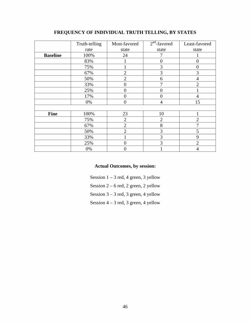
FREQUENCY OF INDIVIDUAL TRUTH TELLING, BY STATES

Truth-telling rate

Most-favored state

2nd-favored state

Least-favored state

Baseline 100% 24 7 1 83% 1 0 0 75% 1 3 0 67% 2 3 3 50% 2 6 4 33% 0 7 2 25% 0 0 1 17% 0 0 4 0% 0 4 15

Fine 100% 23 10 1 75% 2 2 2 67% 2 8 7 50% 2 3 5 33% 1 3 9 25% 0 3 2 0% 0 1 4

Actual Outcomes, by session:

Session 1 – 3 red, 4 green, 3 yellow

Session 2 – 6 red, 2 green, 2 yellow

Session 3 – 3 red, 3 green, 4 yellow

Session 4 – 3 red, 3 green, 4 yellow

46