On Non-Nash Equilibria

Games and Economic Behavior 27, 184–203 (1999)Article ID game.1998.0664, available online at http://www.idealibrary.com on

On Non-Nash Equilibria

Mario Gilli ∗; †

King’s College, CB2 1ST, Cambridge, United Kingdom andUniversita Bocconi, 20136 Milano, Italy

Received February 22, 1996

I consider generalisations of the Nash equilibrium concept based on the idea thatin equilibrium the players’ beliefs should not be contradicted, even if they couldpossibly be incorrect. This possibility depends on the information about opponents’behaviour available to the players in equilibrium. Therefore the players’ informa-tion is crucial for this notion of equilibrium, called Conjectural Equilibrium in gen-eral and Rationalizable Conjectural Equilibrium (Rubinstein-Wolinsky 1994) whenthe game and the players’ Bayesian rationality are common knowledge. In this pa-per I argue for a refinement of Rationalizable Conjectural Equilibrium showing bypropositions and by examples how this equilibrium notion works and how the suit-able equilibrium concept depends on the players’ information. Journal of EconomicLiterature Classification Numbers: C72, D83, D82. © 1999 Academic Press

1. INTRODUCTION

“It has always amused me that what the economist calls an equilibriumof behavior, psychologists tend to call frustration.”

—Kenneth E. Boulding, The Welfare Economics of Grants

The literature on the foundations of solution concepts in game the-ory has extensively analysed the possible reasons for Bayesian rationalplayers to play Nash equilibria. From this literature we have learned thatthe Nash equilibrium (or the Correlated equilibrium) behaviour is justi-fied under restrictive common-knowledge assumptions (see e.g., Aumann-

* I would like to thank E. Agliardi, D. Canning, R. Gatti, F. Hahn, M. Li Calzi, and H.Sabourian for their valuable comments, and the seminar participants at Cambridge Universityfor useful general observations. An anonymous referee was very useful finding mistakes andproviding very detailed comments. The usual disclaimers apply.

† E-mail: [email protected]

1840899-8256/99 $30.00Copyright © 1999 by Academic PressAll rights of reproduction in any form reserved.

on non-nash equilibria 185

Brandenburger (1995)). Alternative reasons to play Nash equilibria havethen been searched for looking at Nash equilibria as possible steady statesof plausible learning models. But if our attention is driven toward this equi-librium notion, then more general equilibrium concepts become relevantand the crucial aspect becomes the players’ information about opponents’behaviour, since the characterisation of a strategy profile as an equilibriumdepends on the information available to the players in that state. Thereforeto study the notion of equilibrium in game theory, we should study the roleof players’ information in strategic situations.

This analysis can be approached from two points of view: the first isa dynamic approach studying how learning leads to different informationpatterns in equilibrium, the second is a static approach, which takes asgiven the information partition and characterises the possible steady statesof generic learning processes, analysing how different information patternslead to different equilibrium concepts. In this paper I follow this secondstrategy showing how the choice among different equilibrium concepts de-pends on the information the analyst thinks the players have. Similarly towhat is done by standard economic theory with market equilibria, a dy-namic model is informally in the background and I allude to it only tomotivate definitions and results. The general notion of equilibrium I usein this analysis is the concept of Conjectural Equilibrium (CE) and of Ra-tionalizable Conjectural Equilibrium (RCE) (Rubinstein-Wolinsky (1994)).The aim of this paper is to argue for a refinement of RCE and to show thewide applicability of this approach to the analysis of strategic situation. Thisallows to show that Rubinstein-Wolinsky (1994) definition of RCE shouldbe strengthen and that some of their statements should be fitted to the newcontext.

The general notion of CE has been defined in the seventies by Hahnfor general equilibrium models (Hahn (1977) and (1978)), but only veryrecently game theorists have rediscovered this idea in learning models(Fudenberg-Levine (1993) and Kalai-Lehrer (1993)) or in the analy-sis of equilibrium concepts (Rubinstein-Wolinsky (1994)). Earlier gametheoretic definition can be found in Battigalli (1987), in Gilli (1987)and in Battigalli-Guaitoli (1988). After a first version of this paper waswritten, I became aware of Dekel-Fudenberg-Levine (1996) that stud-ies a very similar equilibrium notion, even if their focus is on payoffuncertainty.

The rest of this paper is organised as follows. In Sec. 2, I give thebasic game theoretic notions used in Sec. 3 to define Conjectural Equi-librium and its refinements. Section 4 provides an existence theorem.In Sec. 5, I show the relations between (Strong Rationalizable) Con-jectural Equilibrium and solutions concepts extensively used in gametheory.

186 mario gilli

2. IMPERFECT MONITORING GAMES

First the notation: 1�·� is the set of all probability measures on �·�, thesubscript i means that the object refers to player i, if omitted it denotesa complete profile, −i indicates the players different from i, and −i, idenotes a complete profile with the i component stressed. I will rememberthe notation and the interpretations of the basic definitions for extensivegames (EGs) as given by Osborne-Rubinstein (1994), which are slightlymore general of that in Kreps-Wilson (1982). An EXTENSIVE GAME (EG)is defined by:

EG x= �Hy ιyIiy ui�Ni=1; where

• N denotes the set of players and the cardinality of the set itself,

• H is the set of histories h, which are sequences of players’ actions:h = �ak�Kk=1, where ak is the action taken after the history �al�k−1

l=1 .

• ι is the function that assign to each nonterminal history the playerwhose turn it is;

• Ii is a partition of �h ∈ H � ι�h� = i� and is the set of player i’sinformation sets Ii;

• ui is i’s payoff function: ui:1�Z� → R.

From the previous definitions, we can derive the following sets and func-tions:

• player i’s set of pure strategies Si, the set of player i’s mixed strate-gies 6i x= 1�Si�, and the set of mixed strategy profiles 6 x=⊗i∈N 6i, where⊗

i indicates the product of measures;

• the outcome function that identifies the terminal histories inducedby an n-tuple of strategies s ∈ S: ζ: S→ Z;

• i’s payoff function directly defined of the set of players’ possiblestrategies: ui x= ui ◦ ζ; i.e., ui:1�S� → R.

A STRATEGIC GAME (SG) is then defined by

SG x= �Si; ui�Ni=1:

The usual interpretation of SGs is as simultaneous moves games, i.e., gameswith a bijective outcome function (it is easy to see that an extensive gamehas simultaneous moves if and only if the outcome function is bijective).Rubinstein-Wolinsky (1994) enrich the environment defined by a SG bymeans of a signal function: ηi: S → Mi, with the following interpretation:ηi�s� = mi ∈ Mi is the signal privately observed by i ∈ N when s ∈ S isplayed. In other words the mapping ηi represents player i’s information


on opponents’ behaviour, which by definition could depend on player i’sbehaviour itself. Of course the functional form of ηi must be fitted to thecase under analysis: the specification of ηi reflects player i’s informationpartition as seen by the game theorist. An IMPERFECT MONITORINGGAME (IMG) is defined by

G x= �Si; ui; ηi�Ni=1:

A general analysis of IMGs is in Gilli (1994), while a very similar modelfor repeated game is the object of many Lehrer’s papers (see e.g., Lehrer(1989, 1990, 1991, 1992)). In Gilli (1994) I have shown that it is possible todefine an outcome function without any direct reference to an EG and thatsuch function is originated by a “unique" EG (suitably defined). Thereforeit is meaningful to consider the IMG �Si; ui; ζ�, where ζ is the outcomefunction of the unique EG which gives rise to it.

To simplify the analysis I make the following STRUCTURAL ASSUMP-TIONS:

Assumption 1. The analysis is restricted to the subclass of finite imper-fect monitoring games, that is the sets N , Si, Mi are finite.

As usual, this assumption is useful to avoid further complication in themathematical tools used for the analysis. A first consequence of Assump-tion 1 is the following. Fix a finite number of player N and their purestrategies S. Then the space of IMGs over this form is given by G, and Itake G = RN×S ×RN×S; where for �x; y� ∈ G, x�i; s� is the payoff to playeri under strategy s and y�i; s� is the signal to player i under strategy s. If aspecific signal function ηi for each player is specified, then the space G�ηi�is obtained, and I take G�ηi� = RN×S where for x ∈ G�ηi�, x�i; s� is thepayoff to player i under strategy s.

Assumption 2. The signal is defined to contain all of the informationplayer i receives about opponents’ strategic behaviour. Therefore

ηi�si; s−i� = ηi�si; s′−i� ⇒ ui�si; s−i� = ui�si; s′−i�:This assumption means that after the game each player receive her payoffand hence the signal provides nonless information than the payoff; eachplayer recalls her own move in addition to her signal, and given her moveand signal, player i can compute her payoff.

Using ηi it is possible to define an INFORMATION PARTITION forplayer i as follows: let be Si�mi; si �ηi� x= �s−i ∈ S−i �ηi�si; s−i� = mi�,then

Si�si �ηi� x=(Si�mi; si �ηi�

)mi∈Mi

: (1)

188 mario gilli

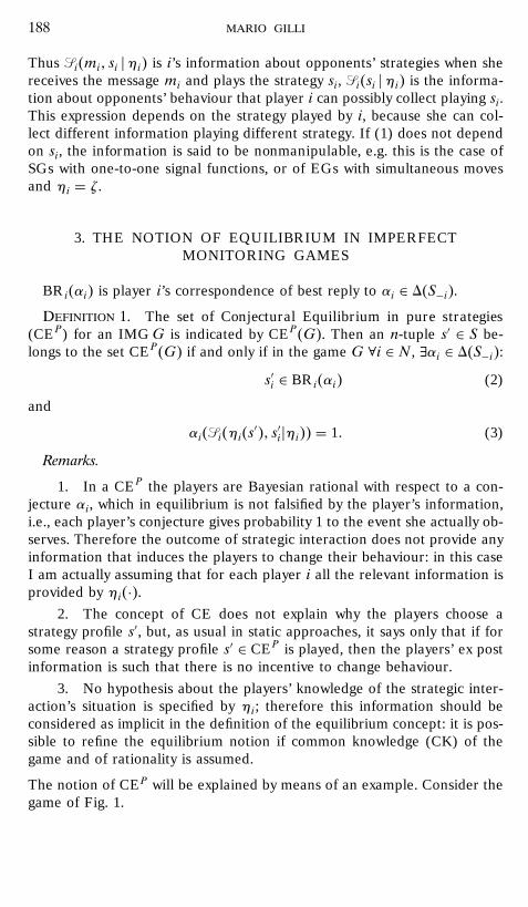
Thus Si�mi; si �ηi� is i’s information about opponents’ strategies when shereceives the message mi and plays the strategy si, Si�si �ηi� is the informa-tion about opponents’ behaviour that player i can possibly collect playing si.This expression depends on the strategy played by i, because she can col-lect different information playing different strategy. If (1) does not dependon si, the information is said to be nonmanipulable, e.g. this is the case ofSGs with one-to-one signal functions, or of EGs with simultaneous movesand ηi = ζ.

3. THE NOTION OF EQUILIBRIUM IN IMPERFECTMONITORING GAMES

BRi�αi� is player i’s correspondence of best reply to αi ∈ 1�S−i�.Definition 1. The set of Conjectural Equilibrium in pure strategies

(CEP) for an IMGG is indicated by CEP�G�. Then an n-tuple s′ ∈ S be-longs to the set CEP�G� if and only if in the game G ∀i ∈ N , ∃αi ∈ 1�S−i�:

s′i ∈ BRi�αi� (2)

and

αi�Si�ηi�s′�; s′i�ηi�� = 1: (3)

Remarks.

1. In a CEP the players are Bayesian rational with respect to a con-jecture αi, which in equilibrium is not falsified by the player’s information,i.e., each player’s conjecture gives probability 1 to the event she actually ob-serves. Therefore the outcome of strategic interaction does not provide anyinformation that induces the players to change their behaviour: in this caseI am actually assuming that for each player i all the relevant information isprovided by ηi�·�.

2. The concept of CE does not explain why the players choose astrategy profile s′, but, as usual in static approaches, it says only that if forsome reason a strategy profile s′ ∈ CEP is played, then the players’ ex postinformation is such that there is no incentive to change behaviour.

3. No hypothesis about the players’ knowledge of the strategic inter-action’s situation is specified by ηi; therefore this information should beconsidered as implicit in the definition of the equilibrium concept: it is pos-sible to refine the equilibrium notion if common knowledge (CK) of thegame and of rationality is assumed.

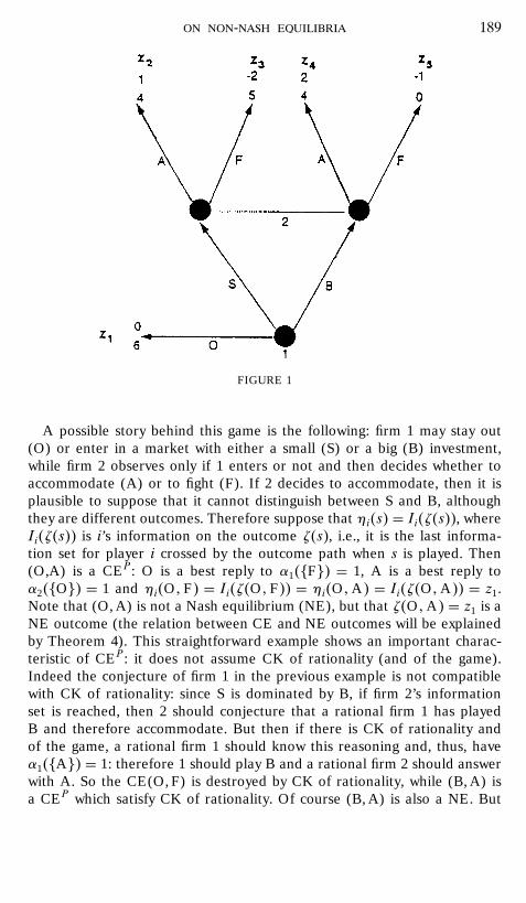
The notion of CEP will be explained by means of an example. Consider thegame of Fig. 1.


FIGURE 1

A possible story behind this game is the following: firm 1 may stay out(O) or enter in a market with either a small (S) or a big (B) investment,while firm 2 observes only if 1 enters or not and then decides whether toaccommodate (A) or to fight (F). If 2 decides to accommodate, then it isplausible to suppose that it cannot distinguish between S and B, althoughthey are different outcomes. Therefore suppose that ηi�s� = Ii�ζ�s��, whereIi�ζ�s�� is i’s information on the outcome ζ�s�, i.e., it is the last informa-tion set for player i crossed by the outcome path when s is played. Then(O,A) is a CEP : O is a best reply to α1��F�� = 1, A is a best reply toα2��O�� = 1 and ηi�O;F� = Ii�ζ�O;F�� = ηi�O;A� = Ii�ζ�O;A�� = z1.Note that (O, A) is not a Nash equilibrium (NE), but that ζ�O;A� = z1 is aNE outcome (the relation between CE and NE outcomes will be explainedby Theorem 4). This straightforward example shows an important charac-teristic of CEP : it does not assume CK of rationality (and of the game).Indeed the conjecture of firm 1 in the previous example is not compatiblewith CK of rationality: since S is dominated by B, if firm 2’s informationset is reached, then 2 should conjecture that a rational firm 1 has playedB and therefore accommodate. But then if there is CK of rationality andof the game, a rational firm 1 should know this reasoning and, thus, haveα1��A�� = 1: therefore 1 should play B and a rational firm 2 should answerwith A. So the CE(O, F) is destroyed by CK of rationality, while (B, A) isa CEP which satisfy CK of rationality. Of course (B, A) is also a NE. But

190 mario gilli

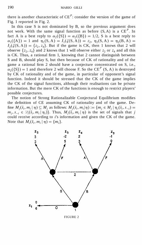
there is another characteristic of CEP : consider the version of the game ofFig. 1 reported in Fig. 2.

In this case S is not dominated by B, so the previous argument doesnot work. With the same signal function as before (S, A) is a CEP . Infact A is a best reply to α2��S�� = α2��B�� = 1/2, S is a best reply toα1��A�� = 1 and η1�S;A� = I1�ζ�S;A�� = z2, η2�S;A� = η2�B;A� =I2�ζ�S;A�� = �z2; z4�. But if the game is CK, then 1 knows that 2 willobserve �z2; z4� and 2 knows that 1 will observe either z2 or z4 and all thisis CK. Thus, a rational firm 1, knowing that 2 cannot distinguish betweenS and B, should play S, but then because of CK of rationality and of thegame a rational firm 2 should have a conjecture concentrated on S, i.e.,α2��S�� = 1 and therefore 2 will choose F. So the CEP �S;A� is destroyedby CK of rationality and of the game, in particular of opponent’s signalfunction. Indeed it should be stressed that the CK of the game impliesthe CK of the signal functions, although their realisations can be privateinformation. But the mere CK of the functions is enough to restrict players’possible conjectures.

The notion of Strong Rationalizable Conjectural Equilibrium modifiesthe definition of CE assuming CK of rationality and of the game. De-fine Mj�si;mi �η� ⊆Mj as follows: Mj�si;mi�η� x= �mj ∈Mj �ηj�si; s−i� =mj; s−i ∈ Si�si;mi �ηi��. Thus, Mj�si;mi �η� is the set of signals that jcould receive according to i’s information and given the CK of the game.Note that Mi�si;mi �η� = �mi�.

FIGURE 2


Definition 2. Fix a game G ∈ G. The set of Strong RationalizableConjectural Equilibria in pure strategies (SRCEP) of game G is denotedby SRCEP�G�. For any i ∈ N , let BPi �mi;G� ⊆ Si be defined as follows:si ∈ BPi �mi;G� if and only if

∃αi�si� ∈ 1( ⋃m−i∈M−i�si;mi�η�

BP−i�m−i;G�)

: (4)

si ∈ BRi�αi�si�� (5)

αi�si�(Si�si;mi �ηi�

) = 1 : (6)

Then an n tuple s′ ∈ S belongs to SRCEP�G� if and only if in the gameG ∀i ∈ N

s′i ∈ BPi �ηi�s′�;G� and mi = ηi�s′�: (7)

Remarks.

1. The expressions (4) and (5) are conditions of Bayesian rationalityunder the assumption of CK of the game and of Bayesian rationality, whileexpressions (6) and (7) are the usual equilibrium condition.

2. Note that in some sense there are three fixed points involved inDefinition 2: two are explicit in conditions (5) and (7), but since the setsBi are defined through the sets B−i, there is a circularity to be solved ei-ther by means of a fixed point argument or through an equivalent iterativedefinition (see Definition 6 and Theorem 1). Consequently the sets BPi andthus SRCEP may easily be empty: existence is proved for mixed SRCE inTheorem 2.

The notion of Rationalizable Conjectural Equilibrium (RCE) has been firstproposed by Rubinstein-Wolinsky (1994), but in their paper they do notstress that under the assumption of CK of the game and of rationality, theplayers’ conjectures should be functions of the strategy the players them-selves choose. RCE can be defined as follows:1

Definition 3. Fix a game G ∈ G. The set of Rationalizable ConjecturalEquilibria in pure strategies (RCEP) of game G is denoted by RCEP�G�.For any i ∈ N , let QPi �mi;G� ⊆ Si be defined as follows: si ∈ QPi �mi;G� ifand only if

∃αi ∈ 1( ⋃m−i∈M−i

QP−i�m−i;G�)

: (8)

si ∈ BRi�αi� (9)

αi(Si�si;mi �ηi

) = 1: (10)

1 The definition given by Rubinstein-Wolinsky (1994) is different, but equivalent.

192 mario gilli

Then an n tuple s′ ∈ S belongs to RCEP�G� if and only if in the gameG ∀i ∈ N

s′i ∈ QPi(ηi�s′�;G

)and mi = ηi�s′�: (11)

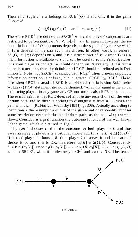
Therefore RCEP are defined as SRCEP where the players’ conjectures arerestricted to be constant, i.e., ∀i, ∀siαi�si� = αi. In general, however, the ra-tional behaviour of i’s opponents depends on the signals they receive whichin turn depend on the strategy i has chosen. In other words, in general,M−i�si;mi �η� depends on si and it is a strict subset of M−i: when G is CKthis information is available to i and can be used to refine i’s conjectures,thus even player i’s conjecture should depend on i’s strategy. If this fact istaken into account, then the definition of RCE should be refined as in Def-inition 2. Note that SRCEP coincides with RCEP when a nonmanipulableinformation partition is defined, but in general SRCEP ⊆ RCEP . There-fore when SRCE instead of RCE is considered, the following Rubinstein-Wolinsky (1994) statement should be changed: “when the signal is the actualpath being played, in any game any CE outcome is also RCE outcome : : : :The reason again is that RCE does not impose any restrictions off the equi-librium path and so there is nothing to distinguish it from a CE when thepath is known” (Rubinstein-Wolinsky (1994), p. 306). Actually according toDefinition 2 the assumption of CK of the game and of rationality imposessome restriction even off the equilibrium path, as the following exampleshows. Consider as signal function the outcome function of the well knownSelten game, which is pictured in Fig. 3.

If player 1 chooses L, then the outcome for both player is L and thusevery strategy of player 2 is a rational choice and thus α1�L� ∈ 1��U;D��.If instead player 1 chooses R, then player 2 observes it and her rationalchoice is U , and this is CK. Therefore α1�R� ∈ 1��U��. Consequently,L 6∈ BR1�α1�L�� since u1�L;α1�L�� = 2 < u1�R;α1�R�� = 3. Thus, �L;D�is not a SRCEP , while it is obviously a CEP and even a NE. The reason

FIGURE 3


for this result is that in many cases the assumption of CK of game andrationality is sufficient to refine the set of possible conjectures even off theequilibrium path, while CE and NE do not fully exploit this assumption, CEbecause it does not assume CK of anything and NE because it is definedon the strategic form and therefore consider any strategic situation as if ithad simultaneous moves and perfect monitoring and thus a nonmanipulableinformation partition.

The extension of these definitions to the case of mixed strategies (and,thus, of distributions over signals) is easy. Define as follows the probabil-ity distribution induced over Mi by a probability measure α ∈ 1�S�:∀mi ∈Mi pi�miyα� x=

∑�s �ηi�s�=mi� α�s�: Denote a generic distribution of prob-

ability on Mi by ρi ∈ 1�Mi�. Then it is possible to define i’s informationpartition derived from ρi and σi:

S mi

(σi; ρi �ηi

) x= {σ−i ∈ 6−i �pi�σi; σ−i� = ρi} ⊆ 6−i:Note that player i’s partition is defined through the probability distributionρi ∈ 1�Mi�, but this does not mean that the players necessarily observe thedistribution of signals induced by the players’ mixed strategy: the fact isthat if the players conjectured distribution is different from the actual one,then in the long run the players will find that they are wrong adjusting con-sequently their conjectures. Moreover, note that 6−i is a simplex in Rk forsome finite k, and that S m

i �σi; ρi �ηi� belongs to the Borel sigma-algebraof Rk since pi�σi; σ−i� is continuous in σ−i: therefore it is meaningfulto write about the probability of S m

i �σi; ρi �ηi�. Define Mmj �σi; ρi �η� ⊆

1�Mj� as follows: Mmj �σi; ρi �η� x= �ρj ∈ 1�Mj� �pj�σi; σ−i� = ρj; σ−i ∈

S mi �σi; ρi �ηi��: Thus, Mm

j �σi; ρi �η� is the information that j could re-ceive according to i’s information and given the CK of the game.

Definition 4. The set of Conjectural Equilibria in mixed strategies(CE) of game G is denoted by CE�G�. Then an n-tuple σ ∈ 6 belongsto the set CE�G� if and only if in the game G ∀i ∈ N , ∃µi ∈ 1�6−i�:

σi ∈ BRi�µi� (12)

µi(S mi �σi; pi�σ� �η�

) = 1; (13)

with the obvious meaning of the abuse of notation in BRi�·�.

Definition 5. Fix a game G ∈ G. The set of Strong RationalizableConjectural Equilibria in mixed strategies (SRCE) of game G is denotedby SRCE�G�. For any i ∈ N , let Bi�ρi;G� ⊆ 6i be defined as follows:

194 mario gilli

σi ∈ Bi�ρi;G� if and only if

∃µi�σi� ∈ 1( ⋃ρ−i∈Mm

−i�σi;ρi �η�B−i�ρ−i;G�

): (14)

σi ∈ BRi�µi�σi�� (15)

µi�σi�(S mi �σi; ρi �ηi�

) = 1: (16)

Then an n-tuple σ ′ ∈ 6 belongs to SRCE�G� if and only if in the gameG ∀i ∈ N

σ ′i ∈ Bi�pi�σ ′�;G� and ρi = pi�σ ′�: (17)

As in Definition 2, SRCE are defined through three fixed points, thereforenonemptiness is not trivial to prove, as Theorem 2 will show.

4. EXISTENCE OF STRONG RATIONALIZABLECONJECTURAL EQUILIBRIA

As shown by the example of Figure 3 it is not true that in general NE ⊆SRCE, while NE ⊆ RCE. Therefore it is not possible to use the Nashexistence theorem to prove that SRCE is not empty and I should followan alternative route. First I prove that the definition of SRCE is equivalentto the requirement that each player can construct a hierarchy of strategysets such that each strategy is rationalised by the next level beliefs, giventhe signal received and given CK of the game and of Bayesian rationality.Then I use this alternative definition of SRCE to show that SRCE 6= Z.

Definition 6. Define: B′i�ρi;G� x=⋂t≥1 B

′i�t; ρi;G� where B′i�0; ρi;G�

x= 6i and ∀t ≥ 1 σi ∈ B′i�t; ρi;G� if and only if

σi ∈ B′i�t − 1; ρi;G� and

∃µi�σi� ∈ 1( ⋃ρ−i∈Mm

−i�σi;ρi �η�B′−i�t − 1; ρ−i;G�

):

σi ∈ BRi�µi�σi�� and µi�σi�(S mi �σi; ρi �ηi�

) = 1:

Theorem 1.

∀G ∈ G;∀i ∈ N; ∀ρi ∈ 1�Mi�; Bi�ρi;G� = B′i�ρi;G�:

Proof. Fix a G ∈ G and, for every i ∈ N , a ρi ∈ 1�Mi�. To simplify thenotation omit G.


First I prove that Bi�ρ� ⊆ B′i�1; ρ�. Suppose that σ ′i ∈ Bi�ρ�, then∃µi�σ ′i � ∈ 1�

⋃ρ−i∈Mm

−i�σ ′i ;ρi �η� B−i�ρ−i��: σ ′i ∈ BRi�µi�σ ′i ��. Since, by defini-tion Bi�ρi� ⊆ 6i and 1�⋃ρ−i∈Mm

−i�σ ′i ;ρi �η� B−i�ρ−i�� ⊆ 1�6−i�, then Defini-tion 6 implies that σ ′i ∈ B′i�1; ρi�. Now assume that for all i Bi�ρ� ⊆ B′i�t; ρ�.Then σ ′i ∈ Bi�ρi�, implies that ∃µi�σ ′i � ∈ 1�

⋃ρ−i∈Mm

−i�σ ′i ;ρi �η� B−i�ρ−i�� ⊆1�⋃ρ−i∈Mm

−i�σ ′i ;ρi �η� B′−i�t; ρ−i�� such that: σ ′i ∈ BRi�µi�σ ′i �� and µi�σ ′i �

�S m−i�σ ′i ; ρi �ηi�� = 1; where the inclusion follows from the induction

hypothesis. Therefore σ ′i ∈ B′i�t + 1; ρi� and, thus, Bi�ρi� ⊆ B′i�ρi�.Now suppose that σ ′i ∈ B′i�ρ�. Note that ∀i, ∀t ′ ∈ N, B′i�ρ� ⊆

B′i�t ′ + 1; ρ� ⊆ B′i�t ′; ρ�. Therefore σ ′i ∈ B′i�ρ� implies σ ′i ∈ B′i�t ′ + 1; ρi� ⊆B′i�t ′; ρi�. Then by definition ∃µi�σ ′i � ∈ 1�⋃ρ−i∈Mm

−i�σ ′i ;ρi �η� B′−i�t ′; ρ−i��

such that:

σ ′i ∈ BRi�µi�σ ′i �� and µi�σ ′i �(S mi �σ ′i ; ρi �ηi�

) = 1:

But this is equivalent to the definition of Bi�ρi�, with B′−i�t ′; ρ� as B−i�ρ�.

Remark. From Theorem 1 it is immediate that ∀G ∈ Gσ ′ ∈ SRCE�G�if and only if ∀i ∈ N∃B′i�ρi;G�: σ ′i ∈ B′i�pi�σ ′�;G�:

Theorem 2.

∀G ∈ G SRCE�G� 6= Z:Proof Fix a game G ∈ G and omit G in the notation. The proof is

organised as follows: first I prove that ∀i, ∀ρiB′i�ρi� 6= Z, then I provethat ∃σ ′ such that σ ′ ∈ B′�p�σ ′��. Both results are based on fixed pointtheorems, therefore the proof depends on the properties of the opportunecorrespondences.

Note that ∀iB′i�t + 1; ρ� ⊆ B′i�t; ρ�. Therefore, if I prove (by induction)that ∀t B′i�t; ρ� is nonempty and compact, then B′i�ρ� 6= Z would followfrom the property of a decreasing succession of nonempty compact sets.By definition B′i�0; ρ� = 6i which is nonempty and compact. Suppose that∀i B′i�t; ρ� 6= Z and compact. Then B′i�t + 1; ρ� 6= Z iff ∃σ ′i ∈ B′i�t; ρi�(which is nonempty by the induction hypothesis) such that

∃µi�σ ′i � ∈ 1( ⋃ρ−i∈Mm

−i�σ ′i ;ρi �η�B′−i�t; ρ−i�

): (18)

µi�σ ′i �(S mi �σ ′i ; ρi �ηi�

) = 1 (19)

σ ′i ∈ BRi�µi�σ ′i ��: (20)

Now if there exists a continuous function µi�σi� satisfying conditions (18)and (19), then the maximum theorem would imply that the correspondence

BRi�µi�:6i →→ 6i

196 mario gilli

is upper hemicontinuous with nonempty convex compact values. ThusKakutani theorem would imply the existence of the fixed point (20) andthus that B′i�t + 1; ρ� is nonempty (and compact). Therefore the crucialpoint is to prove that the correspondence µi:6i →→ 1�6−i� satisfyingconditions (18) and (19) has a continuous selection. Now consider thefollowing facts:

1. S mi �σi; ρi �ηi� is lower hemicontinuous (l.h.c.) in σi and in ρi;

since pi�σi; σ−i� is continuous in σi, σ−i;2. �ρj �pj�σi; σ−i� = ρj� is l.h.c. in σ−i; since pj�σi; σ−i� is continu-

ous in σ−i;3. Mm

j �σi; ρi �η� can be written as follows:

Mmj

(σi; ρi �η

) = ⋃σ−i∈S m

i �σi;ρi �ηi�

{ρj �pj�σi; σ−i� = ρj

}:

Therefore facts 1 and 2 and Proposition 11.23 in Border (1985) imply thatMmj �σi; ρi �η� is l.h.c. in σi and in ρi;

4. Fact 3 and Proposition 11.25 in Border (1985) imply thatMm−i�σi; ρi �η� is l.h.c. in σi and in ρi;

5. Fact 4 and Proposition 11.23 in Border (1985) imply that B′i�t; ρi�is l.h.c. in ρi;

6. Facts 4 and 5, Proposition 11.23 in Border (1985) imply that⋃ρ−i∈Mm

−i�σi;ρi �η� B−i�t; ρ−i� is l.h.c. in σi.

Therefore the correspondence µi:6i →→ 1�6−i� satisfying conditions (18)and (19) is l.h.c. Moreover, it has closed convex values: thus by Theo-rem 14.7 in Border (1985) (see also Michael (1956)) has a continuous se-lection. Therefore B′i�ρi� is nonempty and compact. Moreover, B′�ρ� x=×i∈NB′i�ρ� is obviously convex. Finally fact 5, Propositions 11.23 and 11.25in Border (1985) and the continuity of pi�σ� imply that the correspondence

B′�p�:6→→ 6

is l.h.c in σ and have closed convex values. Therefore Theorem 15.4 inBorder (1985) implies that it has a fixed point: ∃σ ′: σ ′ ∈ B′�p�σ ′�� andtherefore SRCE 6= Z.

5. INFORMATION PARTITIONS AND EQUILIBRIUM CONCEPTS

In this Section I will consider the relationships between the notions of(Strong Rationalizable) Conjectural Equilibrium and the classic solutionconcepts, such as NE and Extensive Form Rationalizability (EFR). These


propositions show the prominent role of players’ information partition whenwe want to analyse a strategic situation. It is trivial to see that ∀G ∈ G,NE�G� ⊆ RCE�G� ⊆ CE�G� (Rubinstein-Wolinsky (1994)). More complexare the relationship between SRCE and NE. The previous example of Fig. 3shows that in a subclass of G SRCE is actually a refinement of NE, whilethe following Theorem 3 shows that when the information partition is non-manipulable, e.g., when the signal function is one-to-one, SRCE and NEcoincides.

For fixed N and S, denote the set of signal functions inducing a nonma-nipulable information partition by NM ⊆ RN×S .

Theorem 3.

∀G ∈ G�η ∈ NM� NE�G� = SRCE�G� = CE�G�:Proof. For this class of games it is immediate that NE�G�⊆ SRCE�G�⊆

CE�G�, since in this case SRCE�G� = RCE�G�. Therefore the result isproved showing that for this class of games CE�G� ⊆ NE�G�. Denote thesupport of a probability measure by SUPP� · �. Suppose that σ ′ ∈ CE�G�.Then ∀i ∈ N ∃µi ∈ 1�6−i� such that:

σ ′i ∈ BRi�µi� (21)

µi({σ−i �pi�·yσ ′i ; σ−i� = pi�·yσ ′i ; σ ′−i�

}) = 1: (22)

Consider condition (21), which implies that ∀s′i ∈ SUPP�σ ′i �, ∀si ∈ Si∫ [∑s−i

ui�s′i; s−i�σ−i�s−i�]µi�dσ−i�

≥∫ [∑

s−i

ui�si; s−i�σ−i�s−i�]µi�dσ−i�:

But∫ �∑s−i ui�s′i; s−i�σ−i�s−i��µi�dσ−i� =

∑s−i ui�s′i; s−i�

∫σ−i�s−i�µi�dσ−i�

=∑s−i ui�s′i; s−i�σ−i�s−i�; where

σ−i�s−i� x=∫σ−i�s−i�µi�dσ−i�: (23)

Therefore the previous inequality can be rewritten as follows: ∀s′i ∈SUPP�σ ′i �, ∀si ∈ Si

∑s−i ui�s′i; s−i�σ−i�s−i� ≥

∑s−i ui�si; s−i�σ−i�s−i�; i.e.,

∀σi ∈ 6iui�σ ′i ; σ−i� ≥ ui�σi; σ−i�: (24)

Note that relations (22) and (23) imply that pi� · yσ ′i ; σ−i� = pi� · yσ ′i ; σ ′−i�.Therefore Assumption 2 implies ui�σ ′i ; σ ′−i� = ui�σ ′i ; σ−i� ≥ ui�σi; σ−i�∀σi ∈ 6i because of inequality (24). Moreover since the informa-tion partition is nonmanipulable and relations (22) and (23) hold,

198 mario gilli

then pi� · yσi; σ−i� = pi� · yσi; σ ′−i�. Therefore Assumption 2 impliesui�σi; σ−i� = ui�σi; σ ′−i� and, thus,

∀σi ∈ 6i ui�σ ′i ; σ ′−i� ≥ ui�σi; σ ′−i�; i.e., σ ′ ∈ NE�G�:

The notion of CE requires much less information about opponents’ be-haviour than the notion of NE. It is therefore surprising that both theseconcepts provide the same restrictions on observable behaviour for a quitecomprehensive class of games. A version of this theorem is proved for EGsin Battigalli (1990) and in Fudenberg-Levine (1993), here we provide theopportune version for this more general setting.

Theorem 4. Let N = �1; 2�. Then

∀G ∈ G�ηi = ζ� ζ�NE�G�� = ζ�CE�G��with the obvious meaning of the abuse of notation.

Proof. Since ∀G ∈ G: NE�G� ⊆ CE�G� then it is immediate that ∀G ∈G: ζ�NE�G�� ⊆ ζ�CE�G��. Therefore I need to prove that under the as-sumption of the theorem ζ�CE�G�� ⊆ ζ�NE�G��. Let �σ1; σ2� ∈ CE�G�.Then I should prove that ∃�σ1; σ2� ∈ NE�G�: ζ�σ1; σ2� = ζ�σ1; σ2�. Bydefinition �σ1; σ2� ∈ CE�G� ⇒ ∃µ1 ∈ 1�62� and ∃µ2 ∈ 1�61� such that:

∀s1 ∈ SUPP�σ1� s1 ∈ BR1�µ1� (25)

µ1({σ2 �p1� · y σ1; σ2� = p1� · y σ1; σ2�

}) = 1 (26)

∀s2 ∈ SUPP�σ2� s2 ∈ BR2�µ2� (27)

µ2({σ1 �p2�·y σ2; σ1� = p2�·y σ2; σ1�

}) = 1: (28)

Now define σ2 x=∫σ2 dµ1 and σ1 x=

∫σ1 dµ2. Then (25) and (27) imply:

σ1 ∈ BR1�σ2� and σ2 ∈ BR2�σ1� because∫63−i

∑S3−i

ui�si; s3−i�σ3−i�s3−i�dµi

=∑S3−i

ui�si; s3−i�∫63−i

σ3−i�s3−i�dµi

(by the previous definition)

=∑S3−i

ui�si; s3−i�σ3−i�s3−i� i ∈ �1; 2�:

But, then σ1 ∈ BR1�σ2� and σ2 ∈ BR2�σ1� since according to (26) and (28)and the hypothesis of the theorem σi differs from σi only out of the equi-librium path and the actions out of equilibrium do not affect the expected


utility. Therefore �σ1; σ2� ∈ NE�G�. Moreover by construction σi and σidiffer only out of the equilibrium path and therefore the outcomes shouldcoincide: ζ�σ1; σ2� = ζ�σ1; σ2�.

Note that the conditions N = �1; 2� and ηi = ζ are both relevant: thefirst guarantees that σ3−i is well defined, while if we don’t restrict the pos-sible information partitions then the theorem is trivially false: think e.g.,of ηi = k. On the other hand these are not the most stringent conditionssecuring the realisation equivalence between CE and NE: see Fudenberg-Levine (1993) for results on EG with perfect monitoring of actions.

When the information available during the game is relevant for the out-come of strategic interaction situations, these contexts are usually modelledas EGs. One of the most important solution concept in this case is EFR(see Pearce (1984) and Battigalli (1997); the version of EFR I use is basedon Battigalli’s paper). I need some terminology

• an information set I ′i precedes I ′′i iff ∀h ∈ I ′′i , ∃h ∈ I ′i : h ⊂ h: Thisrelation is denoted by I ′i ≺ I ′′i .

• a conjecture of a player i ∈ N is a probability measure ci ∈ 1�S−i�,• ci reaches I ∈ Ii iff P�I � si; ci� > 0 for some si ∈ Si,• s′i is a I-replacement for si iff si�I ′� = s′i�I ′� ∀I ′ ∈ Ii \ �I�: I 6≺ I ′;

i.e., s′i differs from si only at I and at its followers,

• a consistent updating system for player i, denoted by CUSi, is amapping ci�·�: Ii → 1�S−i� such that ∀I ∈ Ii ci�I� reaches I and

∀I ′; I ′′ ∈ Ii; I′ ≺ I ′′&ci�I ′� reaches I ′′ ⇒ ci�I ′� = ci�I ′′�:

Definition 7. The set of extensive form rationalizable pure strategiesfor an extensive game E, denoted by P(E), is defined inductively as fol-lows: P�E� x= 3i∈N Pi�E�, Pi�E� x=

⋂t≥1 Pi�t; E� Pi�0; E� x= Si; and si ∈

Pi�t + 1; E� iff:

si ∈ Pi�t; E� (29)

and

∃ci�·� ∈ CUSi:∀I ∈ Ii�si; t� (30)

(i) ci�I� ∈ 1�P−i�t; E��(ii) ui�si; ci�I�� ≥ ui�s′i; ci�I�� ∀s′i ∈ Pi�t; E� and I-replacement for si,

where Ii�si; t� is the set of I ∈ Ii reached by si, s−i for some s−i ∈ P−i�t; E�.Roughly, EFR implies weak sequential rationality since it requires that astrategy specifies a best reply at all information sets that can be reachedby that strategy, given a conjecture consistent with the information sets on

200 mario gilli

the equilibrium path. Moreover it is assumed that this procedure is CK andtherefore it is recursively iterated.

Let P�G� be the set of EFR pure strategies of the extensive game Erepresented as an IMG G with information partition ηi = ζE . I prove thatfor this class of games the strategies in SRCEP coincides with the EFRstrategies which are also part of CEP .

Theorem 5.

∀G ∈ G�ηi = ζ� SRCEP�G� = P�G� ∩ CEP�G�:Proof. Fix a game G ∈ G s.t. ηi = ζ: this condition implies that the

signal is public, thus if s′ ∈ SRCEP , then ∀i, j ∈ N , ∀mi, Mj�s′i;mi � ζ� =ζ�s′�.

I will prove first that SRCEP ⊆ P ∩ CEP: Since SRCEP ⊆ CEP , I needto prove only that SRCEP ⊆ P , and this is done by induction. Therefore, Iwant to show first that SRCEP ⊆ P�1� and then that

SRCEP ⊆ P�t� ⇒ SRCEP ⊆ P�t + 1�: (31)

Define Ii�ζ�s′�� as the set of player i’s information sets reached by theoutcome path when s′ is played. If s′ ∈ SRCEP , then ∀i ∈ N s′i ∈ BPi �ζ�s′��.Thus, ∃αi�s′i� ∈ 1�BP−i�ζ�s′�� such that s′i ∈ BRi�αi�s′i�� and

αi�s′i�({s−i �ηi�s′i; s−i� = ζ�s′�

}) = 1: (32)

Now construct a consistent updating system for player i ci�·� as follows:

ci�·� ={αi�s′i� ∀I ∈ Ii�ζ�s′��c′i�·� otherwise;

where c′i ∈ CUSi. Note that

1. ci�·� ∈ CUSi because c′i�·� is a CUS by definition and αi�s′i� satisfiesDefinition 7 ∀I ∈ Ii�ζ�s′��, since condition (32) implies that ∀I ∈ Ii�ζ�s′��P�I � s′i; αi�s′i�� > 0 and αi�s′i� is constant along the equilibrium path;

2. Ii�ζ�s′�� ⊆ Ii�s′i; 1� because by definition

Ii�s′i; 1� x= {I ∈ Ii � ∃s−i ∈ S−i: P�I � s′i; s−i� > 0}

3. ui�s′i; ci�I�� ={ui�s′i; αi�s′i�� I ∈ Ii�ζ�s′��ui�s′i; c′i�I�� otherwise.

Moreover, out of the outcome path the conjectures do not matter for i’spayoff maximisation: therefore ui�s′i; ci�I�� ≥ ui�si; ci�I�� ∀si ∈ Si and I-replacement for s′i and, thus, s′i ∈ P�1�, i.e., SRCEP ⊆ P�1�.


To show implication (31) assume that SRCEP ⊆ P�t�: Now define B�ζ�as the set of fixed point of B�ζ�·��: B�ζ� x= �s′ ∈ S � s′ ∈ BP�ζ�s′��: Sup-pose s′ ∈ SRCEP , then ∀i s′i ∈ Bi�ζ�. Consequently, ∃αi�s′i� ∈ 1�B−i�ζ�� ⊆1�P−i�t�� such that s′i ∈ BRi�αi�s′i�� and αi�s′i��s−i �ηi�s′i; s−i� = ζ�s′�� =1; where the inclusion follows from the induction hypothesis. Now constructa ci�·� in the following way:

ci�·� ={αi�s′i� ∀I ∈ Ii�ζ�s′��c′i�·� otherwise;

where c′i ∈ CUSi is chosen in such a way that s′i ∈ Pi�t + 1�. This is possiblebecause:

1. ci�·� ∈ CUSi because c′i�·� is a CUS by definition and αi�s′i� satisfiesDefinition 7 ∀I ∈ Ii�ζ�s′��, since ∀I ∈ Ii�ζ�s′�� P�I � s′i; αi�s′i�� > 0 andαi�s′i� is constant along the equilibrium path;

2. Ii�ζ�s′�� ⊆ Ii�s′i; t� because by definition

Ii�s′i; t� x={I ∈ Ii � ∃s−i ∈ P−i�t� ⊇ B−i�ζ� ⊇ �s′−i�: P�I � s′i; s−i� > 0

}and, thus, ∀I ∈ Ii�ζ�s′�� ci�I� = αi�s′i� ∈ 1�B−i�ζ�� ⊆ 1�P−i�t��: More-over, it is possible to choose c′i�·� in such a way that ∀I ∈ Ii�s′i; t� \Ii�ζ�s′��c′i�I� ∈ 1�P−i�t��; since this choice is arbitrary;

3. ui�s′i; ci�I�� ={ui�s′i; αi�s′i�� I ∈ Ii�ζ�s′��ui�s′i; c′i�I�� otherwise.

Therefore there exists a c′i�I� such that ui�s′i; ci�I�� ≥ ui�si; ci�I�� ∀si ∈Pi�t� and I-replacement for s′i and, thus, s′i ∈ Pi�t + 1�.

Now I want to prove that P ∩CEP ⊆ SRCEP: Some preliminary remarksare necessary. First note that the iterative Definition 6 of SRCE can triviallybe specialised to the case of pure strategies. Therefore s′ ∈ SRCEP iff∀t ≥ 1s′ ∈ B′�t; ζ�s′��. Now define B′�t; ζ� as the set of fixed point ofB′�t; ζ�·��: B′�t; ζ� x= �s′ ∈ S � s′ ∈ B′�t; ζ�s′��: Therefore the inclusionthat I want to prove is equivalent to ∀t ≥ 1P�t� ∩ CEP ⊆ B′�t; ζ� that Iprove by induction.

Note that P�1� ∩ CEP ⊆ B′�1; ζ� is immediate since CEP = B′�1; ζ�.Moreover note that there are two possibilities: either CEP = SRCEP orCEP ⊃ SRCEP . In the first case the result follows trivially, while in thesecond case the thesis is equivalent to prove P ⊆ SRCEP . Therefore Ineed to prove that P�t� ⊆ B′�t; ζ� ⇒ P�t + 1� ⊆ B′�t + 1; ζ�: Supposethat s′ ∈ P�t + 1�. Therefore ∀i ∈ N ∃ci�·� ∈ CUSi: ∀I ∈ Ii�s′i; t + 1� theconditions of the definition of EFR hold. In particular ∀I ∈ Ii�s′i; t + 1�ci�I� ∈ 1�P−i�t�� ⊆ 1�B′−i�t; ζ�� and s′i is a best reply among I-replacement

202 mario gilli

in P�t� ⊆ B′i�t; ζ�. Note that

1. by definition Ii�ζ�s′�� ⊆ Ii�s′i; t + 1�;2. ∀I ∈ Ii�ζ�s′�� SUPP�ci�I�� ⊆ B′−i�t; ζ� ⊆ Si�s′i; ζ�s′� � ζ� since by

definition any sj ∈ B′j�t; ζ� should be consistent with the public signal ζ�s′�;3. ci�·� ∈ CUSi is constant along the equilibrium path.

Therefore it is possible to pose αi�s′i� x= ci�I� ∀I ∈ Ii�ζ�s′��: Consider thefirst I ∈ Ii�ζ�s′��, i.e., the first information set of player i along the out-come path: from the previous relations s′i ∈ BRi�αi�s′i�� because informa-tion sets with probability zero are irrelevant for maximisation. Moreover byconstruction αi�s′i� ∈ 1�B′−i�t; ζ�� and αi�s′i��Si�s′i; ζ�s′��ζ�� = 1. Therefore,s′i ∈ B′i�t + 1; ζ�s′�� and thus, Pi�t + 1� ⊆ B′i�t + 1; ζ�.

REFERENCES

Aumann, R., and Brandenburger, A. (1995). “Epistemic Conditions for Nash Equilibrium,”Econometrica 63, 1161–1180.

Battigalli, P. (1987). Comportamento razionale ed equilibrio nei giochi e nelle situazioni strate-giche,” unpublished dissertation, Bocconi University, Milano.

Battigalli, P. (1990). “Incomplete Information Games With Private Priors,” mimeo, BocconiUniversity, Milano.

Battigalli, P. (1997). “On Rationalizability in Extensive Games,” J. Econom. Theory 74, 40–61.Battigalli, P., and Guaitoli, D. (1988). “Conjectural Equilibria and Rationalizability in a

Macroeconomic Game with Incomplete Information,” Working Paper 1988-6, Bocconi Uni-versity, Milano.

Border, K. (1985). Fixed Point Theorems with Applications to Economics and Game Theory.Cambridge: Cambridge Univ. Press.

Dekel, E., Fudenberg, D., and Levine, D.K. (1996). “Payoff Information and Self-ConfirmingEquilibrium,” mimeo.

Fudenberg, D., and Levine, D.K. (1993). “Self Confirming Equilibrium,” Econometrica 61,523–546.

Gilli, M. (1987). Metodo Bayesiano e aspettative nella teoria dei giochi e nella teoria economica,unpublished dissertation, Bocconi University, Milano.

Gilli, M. (1994). “Modelling Strategic Interaction: a Case for Imperfect Monitoring Games,”Working Paper 1994-3, Bocconi University, Milano.

Hahn, F. (1977). “Exercises in Conjectural Equilibria,” Scand. J. Econon. 79, 210–226.Hahn, F. (1978). “On Non-walrasian Equilibria,” Rev. Econom. Stud. 45, 1–18.Kalai, E., and Lehrer, E. (1993). “Subjective Equilibrium in Repeated Games,” Econometrica

61, 1231–1240.Kreps, D. and Wilson, R. (1982). “Sequential Equilibrium,” Econometrica 50, 863–894.Lehrer, E. (1989). “Lower Equilibrium Payoffs in Two-Player Repeated Games with Non-

Observable Actions,” Int. J. Game Theory 18, 57–89.Lehrer, E. (1990). “Nash Equilibria of n-Player Repeated Games With Semi-Standard Infor-

mation,” Int. J. Game Theory 19, 191–217.


Lehrer, E. (1991). “Internal Correlation in Repeated Games,” Int. J. Game Theory 19, 431–456.

Lehrer, E. (1992). “On the Equilibrium Payoffs Set of Two Player Repeated Games withImperfect Monitoring,” Int. J. Game Theory 20, 211–226.

Michael, E. (1956). “Continuous Selection. I,” Ann. Math. 63, 361–382.Osborne, M. and Rubinstein, A. (1994). A Course in Game Theory. Cambridge, MA: MIT

Press.Pearce, D. (1984). “Rationalizable Strategic Behavior and the Problem of Perfection," Econo-

metrica 42, 1029–1050.Rubinstein, A., and Wolinsky, A. (1994). “Rationalizable Conjectural Equilibrium: Between

Nash and Rationalizability,” Games Econom. Behavior 6, 299–311.

Documents

On Non-Nash Equilibria