AN EXPERIMENTAL ROCK MECHANICS INVESTIGATION

INTO

SHEAR DISCONTINUITIES AND THEIR INFLUENCE

IN THE

HYDROCARBON RESERVOIR ENVIRONMENT

by

BRIAN RONALD CRAW FORD

BSc Geology

(University of Glasgow)

MSc (DIC) Structural Geology and Rock Mechanics

(Imperial College, London University)

Thesis presented for the degree of Doctor of Philosophy

at

The Department of Petroleum Engineering,

Heriot-Watt University,

Edinburgh, UK.

1995

© This copy of the thesis has been supplied on condition that anyone who consults it is understood to recognise that the copyright rests with its author and no quotation from the thesis and no information derived from it may be published without the prior written consent of the author or the University (as may be appropriate).

PAGE NUMBERING AS

ORIGINAL

"If our eye could penetrate the earth

and see its interior from pole to pole,

from where we stand to the antipodes,

we would glimpse with horror a mass

terrifyingly riddled with fissures and

caverns."

Thomas Burnet,

Telluris Theoria Sacra

Amsterdam. Wolters, 1694, p.38.

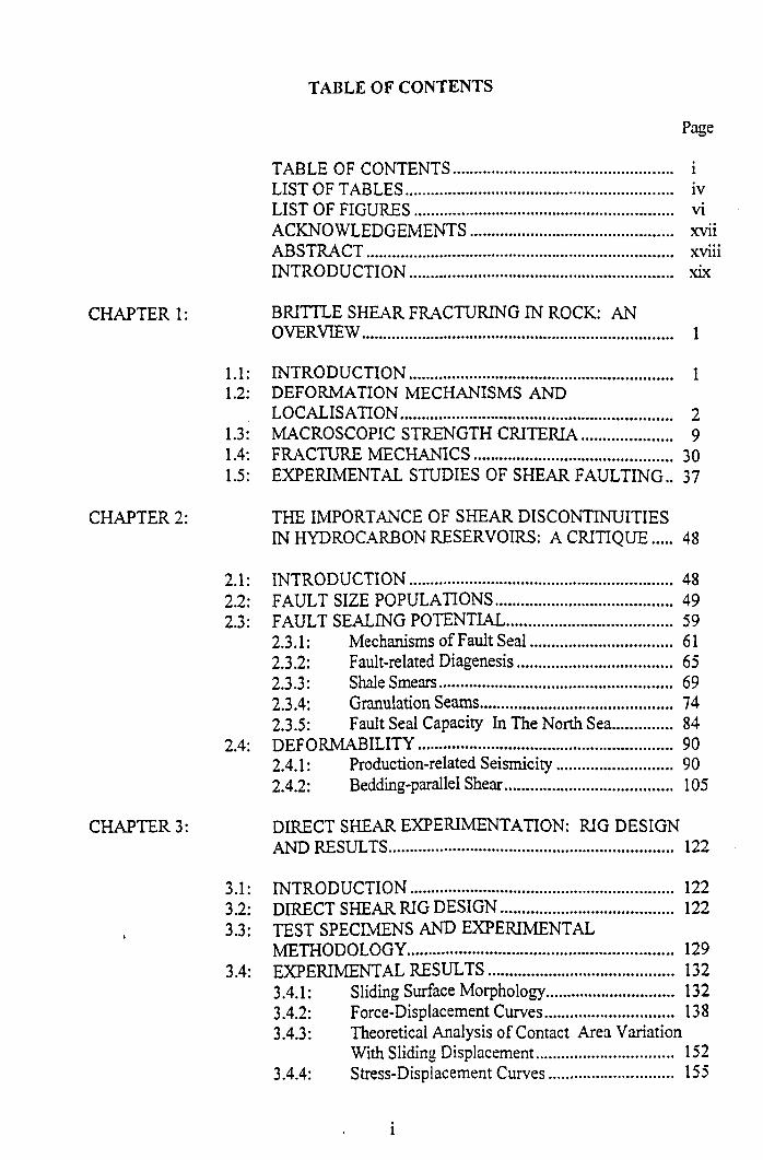
TABLE OF CONTENTS

TABLE OF CONTENTS...................................................... iLIST OF TABLES.................................................................. ivLIST OF FIGURES................................................................ viACKNOWLEDGEMENTS.................................................. xviiABSTRACT............................................................................ xviiiINTRODUCTION................................................................. xix

CHAPTER 1: BRITTLE SHEAR FRACTURING IN ROCK: ANOVERVIEW............................................................................. 1

1.1: INTRODUCTION................................................................ 11.2: DEFORMATION MECHANISMS AND

LOCALISATION.................................................................... 21.3: MACROSCOPIC STRENGTH CRITERIA..................... 91.4: FRACTURE MECHANICS................................................ 301.5: EXPERIMENTAL STUDIES OF SHEAR FAULTING.. 37

CHAPTER 2: THE IMPORTANCE OF SHEAR DISCONTINUITIESIN HYDROCARBON RESERVOIRS: A CRITIQUE..... 48

2.1: INTRODUCTION................................................................ 482.2: FAULT SIZE POPULATIONS........................................... 492.3: FAULT SEALING POTENTIAL........................................ 59

2.3.1: Mechanisms of Fault Seal.................................... 612.3.2: Fault-related Diagenesis........................................ 652.3.3: Shale Smears........................................................... 692.3.4: Granulation Seams................................................. 742.3.5: Fault Seal Capacity In The North Sea................ 84

2.4: DEFORMABILITY.............................................................. 902.4.1: Production-related Seismicity.............................. 902.4.2: Bedding-parallel Shear........................................... 105

CHAPTER 3: DIRECT SHEAR EXPERIMENTATION: RIG DESIGNAND RESULTS....................................................................... 122

3.1: INTRODUCTION................................................................. 1223.2: DIRECT SHEAR RIG DESIGN.......................................... 1223.3: TEST SPECIMENS AND EXPERIMENTAL

METHODOLOGY.................................................................. 1293.4: EXPERIMENTAL RESULTS............................................. 132

3.4.1: Sliding Surface Morphology................................. 1323.4.2: Force-Displacement Curves................................. 1383.4.3: Theoretical Analysis of Contact Area Variation

With Sliding Displacement.................................. 1523.4.4: Stress-Displacement Curves................................ 155

Page

l

Page

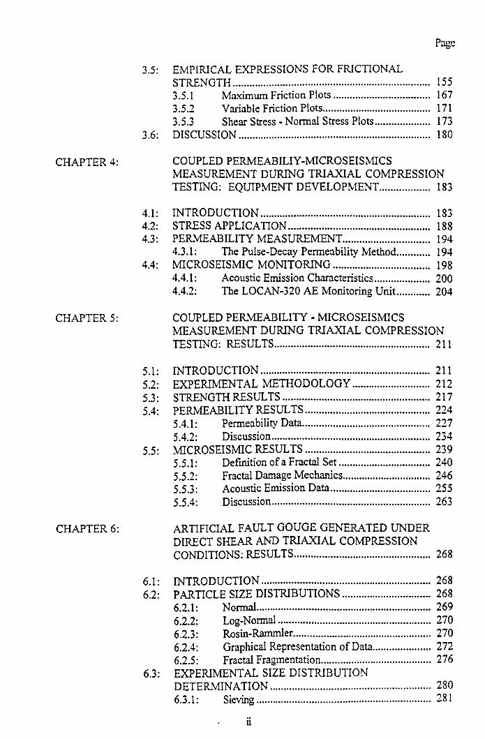
3.5: EMPIRICAL EXPRESSIONS FOR FRICTIONALSTRENGTH............................................................................. 1553.5.1 Maximum Friction Plots..................................... 1673.5.2 Variable Friction Plots......................................... 1713.5.3 Shear Stress - Normal Stress Plots..................... 173

3.6: DISCUSSION.......................................................................... 180

CHAPTER 4: COUPLED PERMEABILIY-MICROSEISMICSMEASUREMENT DURING TRIAXIAL COMPRESSION TESTING: EQUIPMENT DEVELOPMENT................... 183

4.1: INTRODUCTION................................................................. 1834.2: STRESS APPLICATION...................................................... 1884.3: PERMEABILITY MEASUREMENT................................. 194

4.3.1: The Pulse-Decay Permeability Method.............. 1944.4: MICROSEISMIC M ONITORING..................................... 198

4.4.1: Acoustic Emission Characteristics..................... 2004.4.2: The LOCAN-320 AE Monitoring Unit............. 204

CHAPTER 5: COUPLED PERMEABILITY - MICROSEISMICSMEASUREMENT DURING TRIAXIAL COMPRESSION TESTING: RESULTS............................................................ 211

5.1: INTRODUCTION................................................................. 2115.2: EXPERIMENTAL METHODOLOGY............................. 2125.3: STRENGTH RESULTS......................................................... 2175.4: PERMEABILITY RESULTS............................... 224

5.4.1: Permeability Data................................................... 2275.4.2: Discussion............................................................... 234

5.5: MICROSEISMIC RESULTS................................................ 2395.5.1: Definition of a Fractal S et..................................... 2405.5.2: Fractal Damage Mechanics................................... 2465.5.3: Acoustic Emission Data........................................ 2555.5.4: Discussion............................................................... 263

CHAPTER 6: ARTIFICIAL FAULT GOUGE GENERATED UNDERDIRECT SHEAR AND TRIAXIAL COMPRESSION CONDITIONS: RESULTS..................................................... 268

6.1: INTRODUCTION................................................................. 2686.2: PARTICLE SIZE DISTRIBUTIONS.................................. 268

6.2.1: Normal..................................................................... 2696.2.2: Log-Normal............................................................. 2706.2.3: Rosin-Rammler....................................................... 2706.2.4: Graphical Representation o f Data........................ 2726.2.5: Fractal Fragmentation............................................. 276

6.3: EXPERIMENTAL SIZE DISTRIBUTIONDETERMINATION.............................................................. 2806.3.1: Sieving...................................................................... 281

ii

Page

6.3.2: Laser Sizing............................................................ 2826.4: DIRECT SHEAR RESULTS................................................... 288

6.4.1: Sieving Results....................................................... 2896.4.2: Malvern Results.................................................... 2956.4.3: Frictional Strength Correlations and Surface Energy

Considerations....................................................... 3056.5: TRIAXIAL COMPRESSION DEBRIS................................ 317

6.5.1: Shear Band Permeability Estimation................... 3186.5.2: Malvern Results.................................................... 3286.5.3: Sealing Potential Correlation................................ 335

CHAPTER 7: EXPERIMENTAL CONCLUSIONS AND FURTHERANCEOF WORK................................................................................ 339

7.1: CONCLUSIONS........................................................................ 3397.1.1: Direct Shear Experimentation.............................. 3397.1.2: Triaxial Compression Experimentation.............. 3417.1.3: Experimental Fault Gouge Analyses................... 343

7.2: FURTHER WORK........................................!......................... 3467.2.1: Direct Shear Experimentation.............................. 3467.2.2: Triaxial Compression Experimentation.............. 3477.2.3: Experimental Fault Gouge Analyses................... 347

REFERENCES......................................................................... 348APPENDIX 1........................................................................... 370APPENDIX II........................................................................... 383

iii

LIST O F TABLES

Table Page

1.5.1 Summary of studies of localisation' of deformation......................................... 39

2.2.1 Equivalent values of the fractal dimensions of various fault “size”

attributes for a typical ID fault displacement population................................. 55

2.3.4.1 Terms in the published literature synonymous with “granulation

seam” ....................................................................................................................... 76

3.3.1 Specimen lithologies, pre-shear discontinuity descriptions and test variables

for direct shear experimental programme.......................................................... 133

3.5.1 Frictional Strength C riteria ........................................................................ 163

3.5.2 Typical values of variable friction coefficient, for a range of rock types....... 166

3.5.1.1 Maximum friction data for direct shear tests under constant normal

displacement control........................................................................................... 168

3.5.3.1 Frictional sliding constants for direct shear d a ta ............................................... 179

4.4.1 A qualitative comparison of the capabilities of laboratoy shear testing

apparatus............................................................................................................... 184

5.2.1 Geological, poroperm and rock mechanical characteristics of the Clashach

test sand sto n e ................................................................................................. 214

5.2.2 Initial confining pressures for dynamic failure and frictional-sliding, and

final confining pressures for re-shearing................................................. 218

5.4.1.1 Tabulated permeability and associated absolute errors, stress states and

displacements for the seven Clashach triaxial compression experiments.....232

6.2.5.1 Fractal dimensions of a variety of fragmented objects................................278

6.3.1.1 Comparison of U.S.Tyler and B.S.Sieve S eries ............................................... 283

6.4.1 Recovered experimental direct shear fault gouge weights........................... 290

6.4.2 Direct shear specimen percentage mineral contents......................................... 290

6.4.1.1 Direct shear fault gouge distribution characteristics by sieving.................... 291

IV

Table Page

6.4 . 1.2

6.4 .2.1

6.4 .3.1

6.5. 1.1

6.5.1.2

6.5 .2.1

Behaviour of the distribution parameter, n, for various fragmentation methods

............................................................................................................................... 291

Particle size distribution constants derived from laser sizing, for direct shear­

generated fault gouge.............................................................................................303

Harmonic means and specific surface areas for laser-sized direct shear debris

distributions, plus shear fracture energies for those samples exhibiting slip­

weakening ............................................................................................................ 308

Experimental details for shear band thickness calibration specimens #23R and

# 2 4 R ..................................................................................................................... 321

Stress, strain and permeability values for shear bands induced under triaxial

compression........................................................................................................... 321

Tabulated Rosin-Rammler constants for laser-sized gouge distributions . . . . 331

v

LIST O F FIGU RES

Figure Page

1.2.1 Mode of failure transitions in rock ................................................................ 4

1.2.2 Flow diagram illustrating the inter-relationships between lithological

and environmental controls with material processes during rock

deformation..................................................................................................... 4

1.2.3 Review of fracture processes........................................................................ 8

1.3.1 Limits to the dependence of differential stress at shear failure in

compression on confining pressure for a wide range of igneous

rocks................................................................................................................ 13

1.3.2 The Coulomb criterion for shear failure, depicted as a linear Mohr

envelope.......................................................................................................... 13

1.3.3 Andersonian fault classification........................................................... 17

1.3.4 Schematic open crack in compression showing initial extension

directions...........................................................................................................23

1.3.5 The Griffith parabolic failure envelope.......................................................... 24

1.3.6 The combined Griffith-Coulomb failure envelope...................................24

1.3.7 Tensile failure conditions................................................................................. 29

1.3.8 Stress conditions for failure in the negative quadrants of the Griffith

failure envelope................................................................................................. 31

1.3.9 Mohr’s stress circles representing tensile, shear and hybrid tension/

shear fractures................................................................................................ 31

1.4.1 The three basic plane modes of distortion at a crack tip.......................... 33

1.4.2 Co-ordinate frames for analyses of linearly elastic crack tip stress

fields.................................................................................................................. 33

vi

Figure Page

1.5.1 Generalised delineation of four stages in the complete load-displacement

curve of a rock in compression, and corresponding changes in various

physical properties......................................................................................... 42

1.5.2 Curves of stress versus axial strain, lateral strain and volumetric strain

for a brittle rock in a compressive test to failure..........................................42

1.5.3 Schematic diagram showing the propagation of tensile cracks from the

edges of a shear crack in a brittle material....................................................46

1.5.4 Observed fracture types from experimental growth of shear fractures .. 46

2.2.1 Line sampled displacement population curves from a 2D seismic survey

in the North S ea ................................................................................................53

2.2.2 Composite log-log frequency distribution plot of fracture lengths per

unit area of 2D observation plane......................................................... 53

2.2.3 Schematic map showing the positions of randomly distributed barriers

(faults) with a power-law length population..................................................57

2 .2 .4 2D scheme for approximating streamline lengths..................................57

2.2.5 Normalised permeability values computed using the statistical

streamline technique for a variety of power-law size distributions...........60

2.3.1.1 S ummary of controls on fault sealing.............................................................. 62

2 .3 .1 .2 Plot of sealing capacity of different types of fault seal...................................62

2.3.2.1 “Pump” and “valve” models for fluid outflows following shallow

crustal earthquakes........................................................................................... 67

2.3 .2 .2 Schematic model of the seismic valving mechanism for fluid transport

up faults.............................................................................................................67

2.3.3.1 Schematic of a shale smear simple zone analogy........................................... 71

2.3 .3 .2 Schematic of the strained volume of rock associated with normal

fault s lip ............................................................................................................ 71

vu

Figure Page

2.3.3.3 Histogram showing the types of shale smear for the full range of Shale

Smear Factor values...............................................................................73

2.3.4.1 Series of block diagrams showing the sequential development from a

single deformation band to a slip surface..................................................... 77

2 .3 .4 .2 Schematic depicting the relationships between cataclastic slip bands,

cataclastic slip zones and slip surfaces.......................................................... 77

2.3.4.3 General microstructural characteristics in an idealised fault zone..............79

2 .3 .4 .4 Mohr stress diagrams for faults that strain soften and strain harden.......... 79

2.3.4.5 S tress-strain path during failure of a strain-hardening fault....................... 81

2.3 .4 .6 S uccessive Mohr stress circles and failure envelopes for a fault with

rapid transient increase in pore pressure during failure.............................. 81

2.3.5.1 Fault-related seal classification............................................................... 86

2 .3 .5 .2 Parameters contributing to fault seal............................................................... 88

2.4.1.1 Examples of induced changes in stress that can trigger failure in

different faulting environments..................................................................... 92

2 .4 .1 .2 Mohr stress circle for pore pressure induced fault slip..........................92

2.4.1.3 Schematic maps describing the application of the concepts of “barriers”

and “asperities” to explain the seismicity in the Codgell oil field..............97

2.4 .1 .4 Measured surface deformations at Wilmington oil field near Long Beach,

California......................................................................................................... 99

2.4.1.5 Number of earthquakes recorded per year and decline in average

reservoir pressure in two gas fields................................................................ 99

2 .4 .1 .6 Schematic cross-section summarising surface deformation and faulting

associated with fluid withdrawal................................................................... 102

2.4 .1 .7 Calculated change in horizontal normal stress,due to fluid extraction.....102

2.4.2.1 Folding styles....................................................................................................107

2.4 .2 .2 Schematic of the sliding of an overthrust block on a horizontal plane ... . 110

vui

Figure Page

2.4.2.3 Schematic of the shear stress that resists buckling by the flexural slip

mechanism induced by the buckling stress..................................................110

2.4.2.4 Crystal fibres on a flexural slip bedding plane indicating opening as

well as differential bedding slip..........................................................110

2.4.2.5 Bedding slip “squeezing” in the walls of an excavation with associated

upward heave and buckling in the invert.....................................................114

2.4.2.6 Profile along rib faces showing progressive extrusion of individual

soft layers. Differential shearing o f pillars........................................ 114

2.4.2.7 Shear failure of massive roof rock under inferred horizontal

compression, followed by violent shear failure along “cymoidal”

fractures that increase in dip downwards...................................................... 117

2.4.2.8 Relation of common types of rib failures to lithology of roof

rocks, U tah ..................................................................................................117

2.4.2.9 F.E. model of a producing oil reservoir indicating induced

bedding-parallel shear slippage...................................................................... 120

3.1.1 Schematic model of an interbedded rockmass with discontinuities,

consisting of two lithologies, two faults, a joint set and bedding-planes. 123

3.2.1 End view of the direct shear rig parallel to the direction of sliding...........125

3.2.2 Side view of the direct shear rig perpendicular to the direction of

s lid in g ............................................................................................................126

3.2.3 Scaled schematic of the direct shear rig, showing details of the control

system and hydraulics................................................................................... 128

3.4.1.1 Schematic cross-sections illustrating macroscopic specimen deformation on

direct shear of red sandstone, fissile mudrock, carbonaceous siltstone and

heterolithic sandstone/ siltstone lithologies..................................................139

3.4.1.2 Photomicrograph of laboratory direct shear specimen showing

slickenslides, slickenlines and slickensteps................................................ 140

K

Figure Page

3.4.2.1 Schematic diagrams of a typical friction experiment and typical frictional

force as a function of rider displacement results...........................................141

3.4.2.2 Undrained direct shear results with intact and fractured samples of Lyons

sandstone...........................................................................................................141

3.4.2.3 Controlled normal stress and controlled normal displacement direct shearing

modes................................................................................................................ 143

3.4 .2 .4 (a) Idealised relationship between dilation, shear and normal stress with

shear displacement for CNS conditions, and (b) typical pattern of asperity

failure under CNS conditions......................................................................... 145

3.4.2.5 Load-displacement curves for direct shear specimens 3,5 & 6 ................... 148

3.4.2.6 Load-displacement curves for direct shear specimens 8 & 9 ........................149

3.4.2.7 Load-displacement curves for direct shear specimens 11,12 & 14............150

3.4.2.8 Load-displacement curves for direct shear specimens SI, S2, S3 & S 4 .151

3.4.3.1 Geometry for the determination of the area of overlap of two circles with

varying centre displacement.......................................................................... 153

3.4.4.1 Displacement-stress plots for direct shear specimens #3, #5 & #6........... 156

3.4.4.2 Displacement-stress plots for direct shear specimens #8 & #9.............. 157

3.4.4.3 Displacement-stress plots for direct shear specimens #11, #12 & #14 ... 158

3.4 .4 .4 Displacement-stress plots for direct shear specimens SI, S2, S3 & S 4 .. 159

3.5.1.1 Maximum friction plot for direct shear data...................................................170

3.5.2.1 Variable friction versus normal stress plots for the direct shear test data. 172

3.5.3.1 Frictional strength envelopes for direct shear specimens #3, #5 & # 6 .... 174

3.5.3.2 Frictional strength envelopes for direct shear specimens #8 & #9........... 175

3.5.3.3 Frictional strength envelopes for direct shear specimens #11, #12 & #14

.......................................................................................................................... 176

3.5 .3 .4 Frictional strength envelopes for direct shear specimens S 1, S2, S3 & S4

.......................................................................................... 177

x

Figure Page

4.1.1 Schematic representation of coupled permeability - microseismics

experimental testing facility, peripheral to the triaxial compression

configuration................................................................................................... 185

4.1.2 Overview of the triaxial compression system ...............................................187

4.2.1 Applied stress convention in the triaxial compression test.....................189

4.2.2 Block diagram of triaxial test arrangement....................................................189

4.2.3 Principles of operation of the basic closed loop electro-hydraulic servo-

system ............................................................................................................. 193

4.4.1.1 Conventional parameters used to describe an AE signal.............................. 201

4.4.2.1 PAC-supplied calibration curve for the AE transducer used in this study

..........................................................................................................................207

4.4 .2 .2 Scale drawing showing components of AE waveguide........................209

4.4.2.3 Triaxial cell with waveguide and mounted AE transducer, sitting within

stiff compression rig ......................................................................................210

5.2.1 Schematic of experimental programme for triaxial compression testing ..215

5.3.1 Axial load-displacement curves for seven Clashach sandstone specimens

deformed under different confining pressures............................................. 219

5.3.2 Mohr stress circle plots for Clashach sandstone with Coulomb and Griffith

fracture strength envelopes.............................................................................221

5.3.3 Mohr stress circle plots for Clashach sandstone with Coulomb-type

frictional strength envelopes.......................................................................... 221

5.3.4 Clashach sandstone triaxial compression specimens..................................225

5.3.5 Calculated and measured induced fault surface areas versus confining

pressure operative at macroscopic fracture...................................................225

5.4.1.1 (a) Axial permeability versus axial microstrain plots for seven Clashach

specimens, and (b) percentage permeability reduction versus percentage

specimen shortening......................................................................................228

xi

5.4.1.2 Axial permeability versus (a) hydrostatic stress and resolved normal stress

post-dynamic failure, and (b) resolved normal stress post-frictional sliding

and re-shearing...............................................................................................233

5.4.2.1 Schematic illustration of faulted core with shear band inclined to axial flow

direction.......................................................................................................... 236

5.4.2.2 (a) Inverse linear correlation between geometric constant and resolved

normal stress and (b) linear correlation between axial permeability and

Figure Page

geom etric constan t.................................................................................... 238

5.5.1.1 Cantor D ust.......................................................................................................243

5.5.1.2 Sierpinski Carpet.............................................................................................. 243

5.5.1.3 M engor Sponge...........................................................................................243

5.5.2.1 Idealised synoptic model of damage development in a heterogeneous

brittle solid under compression......................................................................249

5.5.2.2 Dependence of crack velocity and event rate on measured stress intensity

KI from double torsion tensile experiments carried out in water at room

temperature......................................................................................................252

5.5.2.3 Variation in b-value (and inferred crack-length distribution exponent, D )

with stress intensity and crack tip “humidity” for a variety of crystalline

rocks.................................................................................................................252

5.5 .2 .4 Synoptic model of the evolution of seismic b-values predicted by

Fig. 5.5.2.3..................................................................................................... 254

6.2.5.1 Self-similar gouge of cubic particles with D = Iog6/log2 = 2 .58....... 279

6.3.2.1 Schematic illustration of the optical configuration employed for laser particle

s iz in g ...............................................................................................................284

6.3.2.2 Properties of scattered light for large and small particles.................... 284

6.4.1.1 Influence of lithology on averaged (a) distribution and (b) absolute size

Rosin-Rammler constants, of sieved direct shear debris............................294

xu

Figure Page

6.4.1.2

6.4.2.1

Ó.4.2.2

6.4.2.3

6.4.2.4

6.4.3.1

6.4.3.2

6.4.3.3

6.4.3.4

6.4.3.5

6.4.3.6

6.4.3.7

6.4.3.8

6.5.1.1

Schematic representation of the micromechanics of fault gouge comminution

associated with macroscopic shearing of (a) quartzose granular and (b)

phyllosilicate-rich rocks..................................................................................297

Distribution functions for red sandstones #3, #5 & # 6 ..............................299

Distribution functions for fissile mudstones #8 & #9 ................................. 300

Distribution functions for carbonaceous siltstones #11, #12 & # 1 4 ........301

Distribution functions for heterolithics S I, S2, S3 & S4....................... 302

Empirical correlation between coefficient of sliding friction and inferred

fractal dimension............................................................................................. 306

Empirical correlation between inferred fractal dimension and specific surface

area.................................................................................................................... 306

Empirical correlation between coefficient of sliding friction and specific

surface area .................................................................................................309

Stress and slip distributions near a crack tip with a breakdown zone in

which the deformation behaviour is governed by the slip-weakening relation

........................................................................................................................... 312

Transformation of post-failure data from an initially intact triaxial

compression test to infer the shear stress versus relative slip relation used in

the slip-weakening m odel..................................................................... 312

Empirical correlation between shear fracture energy and specific surface area

........................................................................................................................... 316

Empirical correlation between shear fracture energy and inferred fractal

dimension............................................................................................... 316

Empirical correlation between shear fracture energy and the coefficient of

sliding friction........................................................................................ 316

Axial stress versus strain curves for Clashach specimens #23 R & #24R 320

xm

Figure Page

6.5.1.2

6.5.1.3

6.5.1.4

6.5.1.5

6.5.2.1

6.5.2.2

6.5.3.1

6.5.3.2

ALI

AI. 2

AI. 3

AI.4

AI.5

AI. 6

AI.7

AI. 8

AI.9

AI. 10

Thin-section photomicrographs of shear bands from Clashach specimens (a)

#23R and (b) #24R ................................................................................ 322

Shear band thickness/slip ratios versus resolved normal stress across the

shear p lane....................................................................................................... 325

Influence of resolved normal stress on (a) shear band permeability and (b)

fault seaing potential....................................................................................... 327

Influence of angular shear strain on (a) shear band permeability and (b)

fault seaing potential........ ............................................................................... 327

Straight-line graphical representations of the Rosin-Rammler function for

laser-sized fault gouge distributions (a) 300mm-range lens (b) 45mm-range

lens.................................................................................................................... 330

Clashach fault gouge "coefficient of variation" versus (a) resolved normal

stress and (b) angular shear strain................................................................. 333

Empirical correlation between the Rosin-Rammler "coefficient of variation"

and (a) shear band permeability and (b) fault sealing potential..............336

Empirical correlation between shear band permeability and fault gouge

specific surface area.........................................................................................336

Red sandstone direct shear specimen #3 sliding surfaces.......................... i

Red sandstone direct shear specimen #5 sliding surfaces.......................... ii

Red sandstone direct shear specimen #6 sliding surfaces.......................... iii

Fissile mudstone direct shear specimen #8 sliding surfaces................. iv

Fissile mudstone direct shear specimen #9 sliding surfaces................. v

Carbonaceous siltstone direct shear specimen #11 sliding surfaces.......... vi

Carbonaceous siltstone direct shear specimen #12 sliding surfaces.......... vii

Carbonaceous siltstone direct shear specimen #14 sliding surfaces.......... viii

Heterolithic direct shear specimen S 1 sliding surfaces........................ix

Heterolithic direct shear specimen S2 sliding surfaces........................x

xiv

Figure Page

AI. 11 Heterolithic direct shear specimen S3 sliding surfaces.......................... xi

AI.12 Heterolithic direct shear specimen S4 sliding surfaces.......................... xii

A ll. 1 Temporal variation in stress, event rate, b-value and D for Clashach

specimen # 1 5 ................................................................................................. i

AIL2 Temporal variation in stress, event rate, b-value and D for Clashach

specimen # 1 6 ................................................................................................. ii

AII.3 Temporal variation in stress, event rate, b-value and D for Clashach

specimen # 1 8 ...................................................................................................iii

AII.4 Temporal variation in stress, event rate, b-value and D for Clashach

specimen # 1 9 .................................................................................................. iv

AII.5 Temporal variation in stress, event rate, b-value and D for Clashach

specimen # 2 0 ................................................................. ................................v

AH. 6 Temporal variation in stress, event rate, b-value and D for Clashach

specimen # 2 1 .................................................................................................. vi

AIL7 Temporal variation in stress, event rate, b-value and D for Clashach

specimen # 2 2 ...................... vii

A ll.8 Stress, event rate, b-value and D versus axial microstrain for Clashach

specimen # 1 5 .................................................................................................. viii

AII.9 Stress, event rate, b-value and D versus axial microstrain for Clashach

specimen # 1 6 .................................................................................................. ix

All. 10 Stress, event rate, b-value and D versus axial microstrain for Clashach

specimen # 1 8 .................................................................................................. x

AH. 11 Stress, event rate, b-value and D versus axial microstrain for Clashach

specimen # 1 9 .................................................................................................. xi

An. 12 Stress, event rate, b-value and D versus axial microstrain for Clashach

specimen # 2 0 .................................................................................................. xii

xv

Figure Page

AIL 13 Stress, event rate, b-value and D versus axial microstrain for Clashach

specimen # 2 1 ..................................................................................................xiii

AIL 14 Stress, event rate, b-value and D versus axial microstrain for Clashach

specimen # 2 2 .................................................................................................. xiv

xvi

ACKNOW LEDGEMENTS

This thesis is dedicated to the memory of Patrick Bradshaw. I wish to acknowledge the

guidance of my supervisor Prof.B.G.D.Smart, and to thank him for instilling in this

"geologist" an appreciation and delight in hydraulics, engineering instrumentation and

control.

This thesis has greatly benefited from the craft and learning of the following experts,

whose contributions are appreciatively acknowledged: Prof.B.G.D.Smart for design of

the direct shear rig and development o f the pulse-decay perm eam eter system;

Dr.I.G.Main for discussion of acoustic emission statistics, his fractal damage mechanics

model, and self-organised criticality; Dr.B.T.Ngwenya for performing XRD analyses of

the direct shear fault gouge; Dr.K.W.McGregor for instruction on operation o f the direct

shear rig; M r.P.W .H.Olden for provision of a finite element model o f reservoir

deformation by bedding-parallel shear slippage.

Contributions from Petroleum Engineering MEng students C.McMeekin (pulse decay

permeability, 1991) and C.Bumside (acoustic emission and micfrofracturing, 1992)

whose theses proved invaluable to this study, are recognised and appreciated.

For stimulating discussion and constructive criticism, I wish to extend heartfelt thanks to

all o f my colleagues in the Rock M echanics R esearch G roup, including

Dr.J.M.Somerville, Mr.J.S.Harper, Ms.S.A.Hamilton and Mr.P.W.H.Olden.

For adroit technical support, Messrs. J.Carlin and A.Winters (Strathclyde University) and

Messrs. D.McLaughlin and CM acleod (Heriot-Watt University) are thanked.

For assistance with typing and for continued support, Ms.J.L.Sewell's contribution is

particularly acknowledged, and finally, for friendship and encouragement I must thank

Dr.R.A.Farquhar and Mr.T.Manzocchi.

xvn

ABSTRACT

Shear fractures are defined in terms of the mechanism and homogeneity of deformation,

macroscopic strength criteria and fracture mechanics parameters. The significance of

shear discontinuities (encompassing both faults and planes of weakness reactivated in

shear) within the hydrocarbon reservoir environment is emphasised with regard to both

petrophysical properties (sealing potential) and controls on reservoir deformation, and an

experimental rock mechanics programme has been undertaken to study fundamental

aspects of their frictional strength and permeability. The design of a new direct shear rig

is described, and initial results presented from a suite of experiments conducted under

constant normal displacement control, analogous to ultra-stiff wall rock conditions. Load-

displacement data for a variety of sedimentary lithologies, is analysed in terms of the

mechanism of frictional sliding, with slip on induced wear debris (fault gouge) being

found to conform to a simple linear strength law. A coupled permeability measurement

and microseismics monitoring facility, for studying the influence of microstructural

deformation on fluid flow under varying triaxially compressive stress states, is described.

Data is presented for discrete failure and frictional sliding tests on a homogeneous

sandstone. A method for estimating induced shear band permeability from axial core plug

measurements is outlined. Computed permeability reductions range from 2.5 to 3.5 orders

of magnitude, with shear band sealing exhibiting an order of magnitue increase with

increasing resolved normal stress and angular shear strain. Acoustic emission is described

using an existing fractal damage mechanics theory for fault nucleation, and suggests a

condition of self-organised criticality during frictional sliding. Collected fault gouge from

the direct shear and triaxial compression specimen suites has been analysed using both

sieving and laser particle-sizing methods. Measured cumulative weight distributions are

described using the Rosin-Rammler exponential function, implying fractal size-scaling.

Correlations are presented between distribution constants and: (i) frictional resistance

(coefficient of sliding friction and shear fracture energy) from direct shear testing; (ii)

fluid flow (permeability and sealing potential) from triaxial compression testing. Such

relations may reflect that portion of the total strain energy allocated to the creation of new

surface area.

xviii

INTRODUCTION

The common reservoir engineering concept of a naturally fractured reservoir envisages a

"sugar-cube" geometry in which the fractures are of infinite extent, constant aperture and

regular spacing, and furthermore, the classification "naturally fractured" usually refers to

those reservoirs in which open joints provide the major proportion of the effective

permeability for fluid production. Whilst volumetrically, tectonic features generally

contribute very little to the total porosity of a reservoir, the matrix porosity between

tectonic surfaces is only effective porosity if these discontinuities do not possess reduced

permeability characteristics. Although developments in probe permeametry have enabled

quantification of sedimentary heterogeneity down to the lamina-scale, no parallel advance

has been evident in similarly quantifying the flow characteristics o f tectonic

discontinuities which overprint the stratigraphy. To fully incorporate fault architecture

into reservoir simulation model gridblocks, reliable predictions of their size population,

spatial distribution, geometry and hydraulic characteristics are a prerequisite. However,

although structural geological observations reveal small-scale faulting to be common in

high porosity reservoir sandstones, the petrophysical properties and sealing characteristics

of such tectonic surfaces remain surprisingly the least quantified of the above physical

attributes. Also, reservoir deformation accommodated by slippage on shear

discontinuities associated with production-related transients in in situ stress, is postulated

to have major detrimental repercussions with respect to such phenomena as induced-

seismicity and well casing-failure. In particular, the mechanism of bedding-parallel shear

is highlighted, in which flexure above a compacting and subsiding reservoir generates

excess shear stresses in the overburden, that can result in horizontal shear failure and

slippage along weak lithologies such as shale intercalations.

Accordingly, an experimental rock mechanics programme has been undertaken expressly

to study pertinent fundamental properties of shear discontinuities, including specifically

frictional resistance and permeability. This study has focused in particular on the

development and proving of laboratory equipment and techniques.

xix

In Chapter 1, fundamental properties of brittle deformation are discussed, and shear

fracturing defined in terms of the mechanism and homogeneity of deformation,

macroscopic strength criteria and fracture mechanics parameters. In Chapter 2, the

significance of shear discontinuities within the hydrocarbon reservoir environment is

emphasised with regard to both petrophysical properties resulting in sealing behaviour

and thus reservoir compartmentalisation, and control on production-related reservoir

deformation. In Chapter 3, the design of a new servo-hydraulic direct shear rig is

outlined. Initial load-displacement data generated by a variety of sedimentary lithologies,

sheared under optimum frictional wear conditions corresponding to maximum

suppression of discontinuity-normal dilation, is expressed in terms of a frictional strength

law. In Chapter 4, a combined liquid permeameter and microseismics monitoring system,

peripheral to a conventional rock mechanics servo-hydraulic triaxial compression

configuration, is detailed, capable of quantifying fluid flow potential associated with

microstructural deformation resulting from applied stress states. In Chapter 5, strength,

acoustic emission and permeability results for compressive triaxial stresses ranging from

hydrostatic to dynamic failure to frictional sliding conditions, are presented. Acoustic

emission is quantified in terms of an existing fractal damage mechanics model, and a

means of estimating shear band permeability from transient whole core measurements is

outlined. In Chapter 6, experimentally-generated frictional wear products (fault gouge)

resulting from both the direct shear and triaxial compression test programmes, are

analysed using conventonal sieve and laser particle-sizing techniques. Small particle

statistical parameters are used to describe the debris distributions, and are correlated with

both frictional resistance and fluid flow. In Chapter 7, general experimental conclusions

and recommendations for continuation of related research are elaborated.

xx

1. BRITTLE SHEAR FRACTURING IN ROCK: AN OVERVIEW

1.1 INTRODUCTION

In this introductory chapter, brittle rock deformation and the various processes leading

ultimately to shear localisation resulting in the formation of shear bands commonly

referred to as faults, are reviewed. Macroscopic strength criteria representing both

theoretical and empirical relationships between principal stresses on shear failure are

contrasted with fracture mechanics theory describing the relationships between crack tip

stresses and propagation modes. Both approaches are finally reconciled via a discussion

of fracture criteria in the light of experimental results, which show that macroscopic shear

fractures form by the coalescence of tensile microcracks.

In this chapter 1, primary attention is focused on assessing the formation and growth of

shear fractures in rock material from the microscale to the macroscale (faulting). An

important distinction thus exists between this chapter and the succeeding chapter 2, which

deals with the role of shear discontinuities, specifically in the hydrocarbon reservoir

environment. In the latter chapter, not only shear fracturing as discussed in chapter 1 is

indicated (both tectonic shear fractures and "anthroprogenic" ones induced due to

production-related stress changes) but also activation of pre-existing planar features in

shear, such as joints and bedding planes. Thus in this instance, shear discontinuities is

used as an "umbrella-term" encompassing both shear fractures (faults) formed by strain

localisation and the coalescence of microcracks, as well as subsequent shearing of

existing planes of weakness, resulting from a transient in the ambient physical conditions.

Throughout this thesis work fractures will be described as "shear fractures" (equivalent to

"faults") if they exhibit shear displacement, and as "joints" if they are dilational features

which exhibit no shear. Obviously this study is overwhelmingly concerned with the

former fracture type, and will only touch on jointing when it serves to highlight important

differences between the two fracture types such as mode of genesis, physical properties

etc. A cautionary note is made at this stage regarding the increasing tendency in rock

mechanics literature of referring to all planar discontinuities in the rockmass as "joints"

1

irrespective of their mode of displacement. Such a trend is not adhered to in this

discussion.

1.2 DEFORM ATION M ECHANISM S AND LOCALISATION

For a full assessment of the way in which a rock has been deformed, both experimentally

and tectonically in situ, two concepts are essential for a complete description:

(i) deformation mechanism(s) and,

(ii) the degree of homogeneity of the deformation (Rutter, 19861).

Three fundamental deformation mechanisms can operate in rocks:

(i) Cataclasis, in which crystal structure remains undistorted but grains or groups of

grains become cracked and the fragments may exhibit frictional sliding with respect

to one-another. The process necessarily involves dilatancy and as such is pressure

sensitive.

(ii) Intracrystalline plasticity, in which grains become internally distorted through

dislocation motion or deformation twinning.

(iii) Flow by diffusive mass transfer (pressure solution), in which shape change of the

deforming aggregate is achieved by stress induced diffusion of matter away from

interfaces sustaining high normal stresses, with the same or different phases being

re precipitated at potentially dilatant sites.

Whilst (ii) and (iii) can be constant volume processes and hence are relatively pressure

insensitive, both are sensitive to temperature and deformation rate relative to (i).

Deformation can be heterogeneous due to localisation into a band (a brittle fault or ductile

shear zone) in an otherwise homogeneously deforming (or rigid) body. Each o f the above

fundamental mechanisms can result in localised or distributed rock deformation

depending on rock type and physical conditions as well as strain magnitude, localisation

sometimes developing after a certain degree of homogeneous flow. With “brittleness”

2

being unequivocally associated with microcrack formation, and “ductility” defined as the

capacity for more or less uniformly distributed flow, the former is therefore essentially a

mechanistic concept defined at the microscopic level, whilst the latter must be defined at

the macroscopic level and is independent of deformation mechanism. For example, in the

earliest experimental studies on the “brittle to ductile transition” the transition from

localised cataclasis (brittle faulting) to ductility due to distributed microcracking

(cataclastic flow) was observed with increasing confining pressure at constant

temperature. Ductility due to intracrystalline plasticity (deformation by the movement of

dislocations or the twinning of crystals) on the other hand could be achieved

experim entally by the application of yet higher confining pressures, or higher

temperatures, or both. Rutter was particularly concerned by the restricted use of the term

“ductility” which he felt was increasingly being identified purely with deformation by

intracrystalline plasticity and thus being made mechanism dependent, to the exclusion of

cataclastic flow processes. Also, it was stressed that cataclastic flow (cataclasis without

localisation) which may involve microfracturing of every grain in the rock or may

fragment the rock into cm-sized to sub-micron-sized pieces, can accommodate folding via

small movements on homogeneously distributed bounding cracks. Thus in the above

example both brittleness and ductility occur together and the scale of observation needs to

be indicated, in this instance brittle on the grain scale, macroscopically ductile.

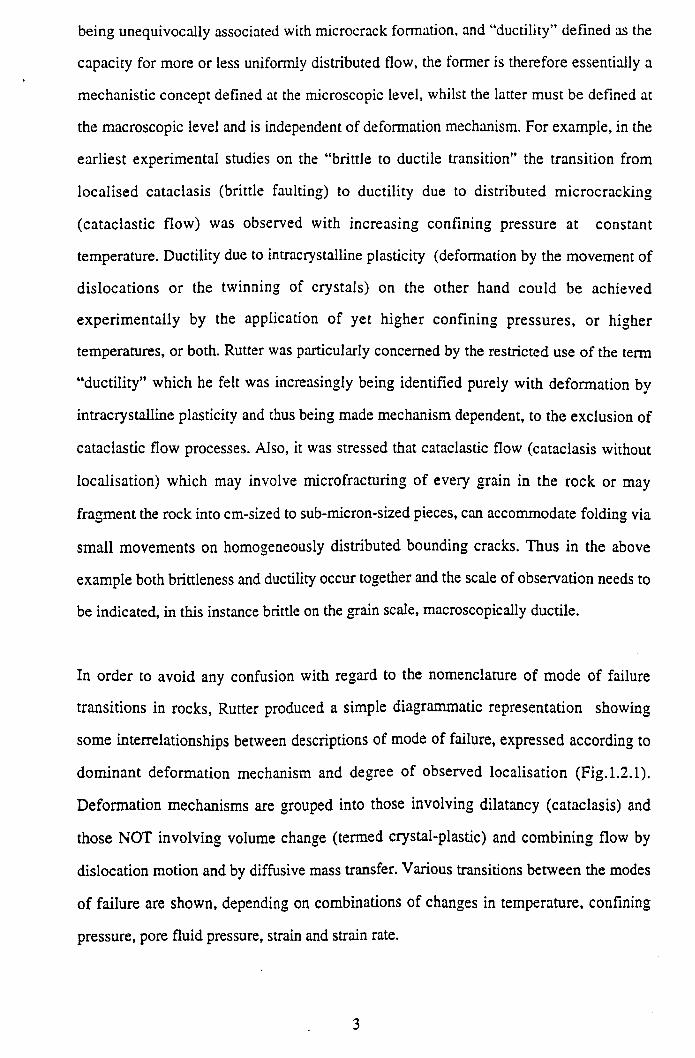
In order to avoid any confusion with regard to the nomenclature of mode of failure

transitions in rocks, Rutter produced a simple diagrammatic representation showing

some interrelationships between descriptions of mode of failure, expressed according to

dominant deformation mechanism and degree of observed localisation (Fig. 1.2.1).

Deformation mechanisms are grouped into those involving dilatancy (cataclasis) and

those NOT involving volume change (termed crystal-plastic) and combining flow by

dislocation motion and by diffusive mass transfer. Various transitions between the modes

o f failure are shown, depending on combinations of changes in temperature, confining

pressure, pore fluid pressure, strain and strain rate.

3

LITHOLOGICALCONTROLS

ENVIRONMENTALCONTROLS

mineralogy, effective stress,grain-size, temperature,porosity, strain rate,permeability etc. fluid chemistry etc.

/¡“ □E 1SELECTION OF DOMINANT

MATERIAL PROCESSES

DEFORMATION MECHANISMS

IRock fabric modification and

generation of new fabric elements

MATERIALPROCESSES

Within grains:1. Diffusion2. Dislocation movement3. Twinning4. Elastic distortion5. Fracture

At grain boundaries:6. Dissolution7. Reaction8. Diffusion9. Crystal growth

10. Fracture11. Frictional sliding 12.Sliding by diffusion or

dislocation processes

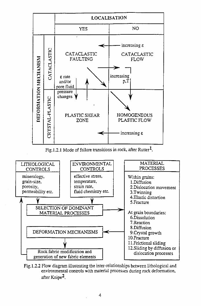
Fig. 1.2.2 Flow diagram illustrating the inter-relationships between lithological and environmental controls with material processes during rock deformation,after Knipe^.

4

Knipe (1989)2 writes that the response of a rock to deformation is a function of a large

number of environmental and lithological variables. Fig. 1.2.2 lists these variables and

outlines the ways in which these factors combine to activate a dominant set of material

processes. The combined material processes operative in a rock under specific

environmental conditions will control the deformation mechanisms which operate and

thus the resultant microstructures which evolve. Knipe separates brittle deformation

processes into:

(i) frictional grain-boundary sliding where fracture does not dominate the deformation

and,

(ii) fracture processes.

Knipe writes that deformation by frictional grain-boundary sliding leaves individual

grains essentially undeformed, with instead grains acting as rigid bodies and sliding past

each other. In this respect, sliding commences when the cohesion and frictional resistance

between grains is overcome, and therefore the initiation of sliding is critically dependent

upon the amount and strength of cement bridges between the grains. Frictional grain-

boundary sliding is a pressure sensitive mode of deformation, enhanced by low confining

pressures and high fluid pressures (low effective stresses) and as such is prevalent in

partially or unlithified sediments (Maltman, 19843) and in fault zones containing

incohesive gouges (Wang, 19864). Intergranular frictional sliding has the potential to

involve complex volume changes, where high fluid pressures and fluid influxes promote

significant dilation and even fluidisation and liquefaction of the aggregate (c.f. soft

sediment deformation structures) however late stage fluid losses may eliminate the grain-

scale transient dilation. Large volume losses are also possible in clays and muds

subjected to this deformation process, associated with preferred mineral alignment within

the grain framework due to porosity collapse on fluid expulsion. Such deformation

processes are cited as being responsible for faulting in partially lithified sediments

recovered from DSDP cores. Knipe (1986)5 proposes that fluid migration coupled with

frictional grain-boundary sliding (resulting from fluid overpressuring or the regional

5

stress field) could induce a migrating wavefront of deformation in which the following

sequential process migrates through partially lithified sediments:

dilation + fluid influx —>disaggregation + displacement —» collapse + grain alignment .......... Eqn. 1.2.1

Knipe regards this process involving the migration of fluid “packets” and pressure waves

as being of potential importance in the evolution of bedding fabrics formed during

compaction and in the alignment of clay particles in fault and shear zones.

Fracture processes are concerned with the nucléation, propagation and displacement

along new surfaces created during deformation, Knipe (1989)2 highlighting the fact that

integration of the fracture mechanics approach, which defines the conditions and

processes associated with single crack or fault propagation, has been o f seminal

importance in the interpretation of failure modes and conditions in rock. Some important

applications of fracture mechanics theory, specifically to shear discontinuities in rock,

will briefly be discussed in section 1.4. Fracture processes (in which fracturing dominates

the deformation) also incorporate (or indeed are synonymous with) cataclasis, where

fragmentation of material together with rotation and associated grain-boundary sliding

and dilation, dominate faulting at high crustal levels producing fault gouges and breccias.

The simple classification of fracture mechanisms given below emphasises the range of

pre-failure processes which influence or control the propagation of fractures: (i) Elastic

strain accumulation, where the elastic strain energy associated with a stress concentration

at a crack tip controls propagation. A number of theories are based on quantification of

this stress intensity factor to predict conditions needed for crack extension at tips with

different geometries and under different loads (see section 1.4). Developed fractures tend

to follow microstructural weaknesses in the material and as such may be transgranular

utilising cleavage orientations or intergranular in which case grain-boundaries are

exploited. Thus the frequency, orientation, shape, aspect ratio and distribution of pre-

6

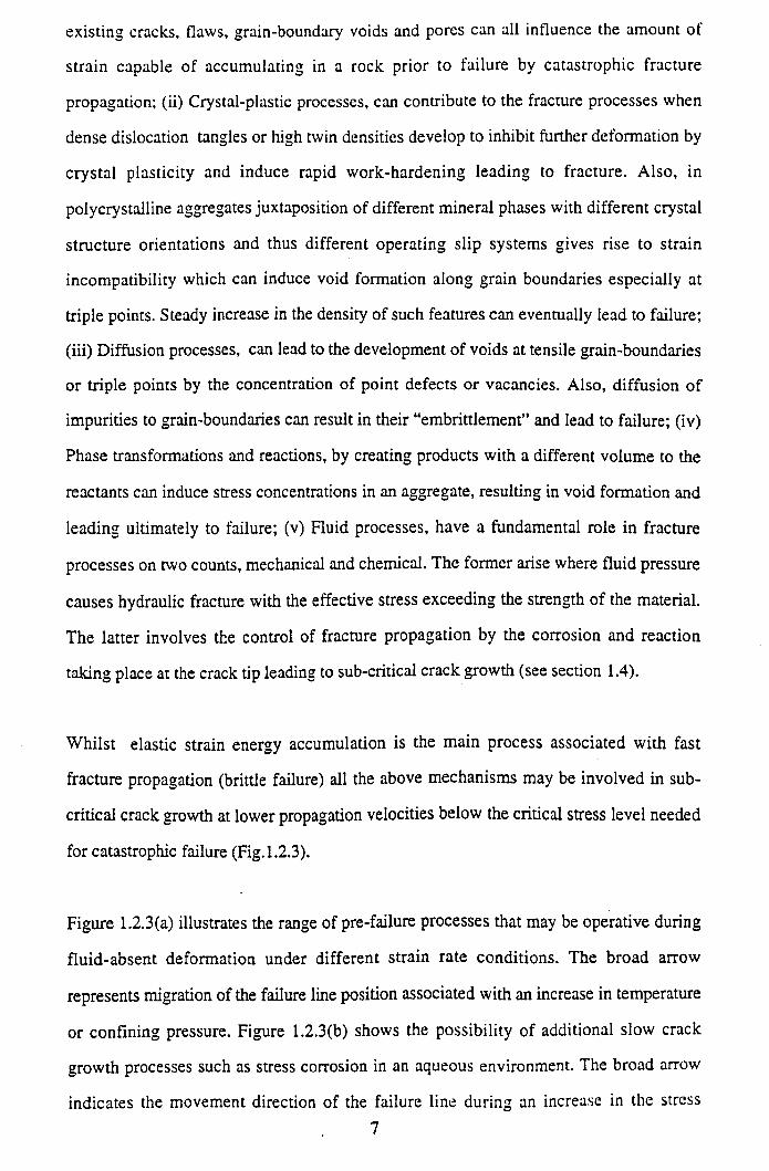
existing cracks, flaws, grain-boundary voids and pores can all influence the amount of

strain capable of accumulating in a rock prior to failure by catastrophic fracture

propagation; (ii) Crystal-plastic processes, can contribute to the fracture processes when

dense dislocation tangles or high twin densities develop to inhibit further deformation by

crystal plasticity and induce rapid work-hardening leading to fracture. Also, in

polycrystalline aggregates juxtaposition of different mineral phases with different crystal

structure orientations and thus different operating slip systems gives rise to strain

incompatibility which can induce void formation along grain boundaries especially at

triple points. Steady increase in the density of such features can eventually lead to failure;

(iii) Diffusion processes, can lead to the development of voids at tensile grain-boundaries

or triple points by the concentration of point defects or vacancies. Also, diffusion of

impurities to grain-boundaries can result in their “embrittlement” and lead to failure; (iv)

Phase transformations and reactions, by creating products with a different volume to the

reactants can induce stress concentrations in an aggregate, resulting in void formation and

leading ultimately to failure; (v) Fluid processes, have a fundamental role in fracture

processes on two counts, mechanical and chemical. The former arise where fluid pressure

causes hydraulic fracture with the effective stress exceeding the strength of the material.

The latter involves the control of fracture propagation by the corrosion and reaction

taking place at the crack tip leading to sub-critical crack growth (see section 1.4).

W hilst elastic strain energy accumulation is the main process associated with fast

fracture propagation (brittle failure) all the above mechanisms may be involved in sub-

critical crack growth at lower propagation velocities below the critical stress level needed

for catastrophic failure (Fig. 1.2.3).

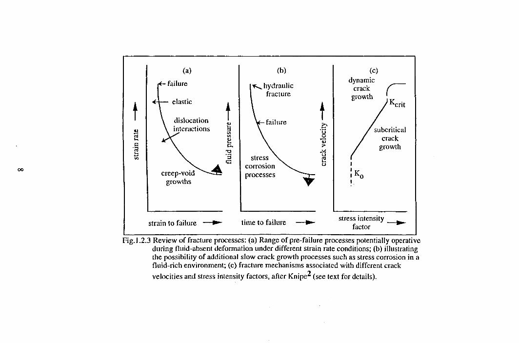
Figure 1.2.3(a) illustrates the range of pre-failure processes that may be operative during

fluid-absent deformation under different strain rate conditions. The broad arrow

represents migration of the failure line position associated with an increase in temperature

or confining pressure. Figure 1.2.3(b) shows the possibility of additional slow crack

growth processes such as stress corrosion in an aqueous environment. The broad arrow

indicates the movement direction of the failure line during an increase in the stress

7

stress intensity factor

Fig. 1.2.3 Review of fracture processes: (a) Range of pre-failure processes potentially operative during fluid-absent deformation under different strain rate conditions; (b) illustrating the possibility of additional slow crack growth processes such as stress corrosion in a fluid-rich environment; (c) fracture mechanisms associated with different crackvelocities and stress intensity factors, after Knipe2 (see text for details).

intensity factor and/or alteration in the fluid chemistry towards a more corrosive

composition. Figure 1.2.3(c) shows the fracture mechanisms associated with different

crack velocities and stress intensity factors. The stress intensity factor. K, equivalent to

the driving force behind crack propagation, describes the stress field at the crack tip and

is dependent on the loading conditions and material properties (see section 1.4). K

magnitude ranges from Ko, below which sub-critical crack growth ceases, to Kent, at

which critical level the crack propagates catastrophically to approach the velocity of

sound in the medium.

1.3 M ACROSCOPIC STRENGTH CRITERIA

In section 1.2 above, an attempt is made to understand shear fracturing in rock in terms of

both the mechanism and the homogeneity of deformation. In section 1.4 below fracture

mechanics theory describes the conditions under which an individual crack will propagate

in an elastic medium. It is a continuum mechanics approach in which the crack is

idealised as a mathematically flat and narrow slit in a linear elastic medium. It seeks to

analyse the stress field around the crack and then to formulate a fracture criterion based

on certain critical parameters of the stress field. The macroscopic strength is thus related

to the theoretical, intrinsic strength (that is the strength required to break the bonds across

a lattice plane) of the material through the relationship between the applied stresses and

the crack-tip stresses. However only in one special case, that of tensile fracture of a

homogeneous elastic material, do these theories also predict the macroscopic strength.

Thus in describing the strength of rock under general stress conditions, we are still forced

to use criteria which are empirical or semi-empirical in nature. Such macroscopic fracture

criteria had been well established by the beginning of the twentieth century (Coulomb,

17736, Mohr, 19007) and thus pre-date the theoretical framework underlying fracture

mechanics. A very brief summary of macroscopic strength criteria will be given below as

many rock mechanics texts give detailed descriptions of these (see in particular the

excellent account given in Jaeger & Cook, 19798, pages 95-106). In particular, attention

will be focused on the Griffith criterion (as it possesses the attractive feature of

combining both tensile and shear failure in a single criterion) to gain an understanding of

9

how the various fracture types (both shear and tensile) develop, and how their formation

may be interpreted in terms of crustal stress and fluid pressure conditions.

There is no universal simple law governing the level of stress at which a specific

lithology fractures as this level probably depends on the mode of fracture (tensile or

shear) and also involves all principal stress components. To express the failure conditions

in the most general way, an appropriate function is sought experimentally which has the

three principal stresses, a i>ct2>ct3 as variables, which takes on a certain fixed value for

any combination of the principal stresses at which fracture occurs. This condition, often

written in the form:

Ci = f((J2, 0 3 ) .......... Eqn.1.3.1

is known as a "failure criterion". The function, f, includes at least one variable

characteristic of the material. However, the assumption cannot be made that a particular

failure criterion, f, will necessarily apply to more than one particular mode of fracture,

unless it can be shown that the underlying physical mechanisms are the same. In

particular, it is possible that extension and shear fractures may be controlled by different

criteria o f failure. One such criterion, which experiment shows is generally adequate, is

that tensile failure will occur with parting on a plane normal to the least principal stress,

when that stress is tensile and exceeds some value T, the tensile strength, (Jaeger &

Cook, page 90) thus:

<J3 = -T .......... Eqn. 1.3.2

The accurate determination of the uniaxial tensile strength is notoriously difficult, both

because of the experimental problem of achieving a macroscopically uniform tensile

stress, and because of the inherently large scatter in the tensile strength of most rocks.

Consequently, there is a general preference for obtaining T from an indirect test such as

10

the Brazilian disk method which gives more consistent results, although this approach

rests on certain assumptions about stress distribution (see the discussion in section 6.3.1).

The range of combinations of principal stresses over which the preceding conclusion

(Eqn. 1.3.2) can be tested is severely limited because of the narrow range of confining

pressures in the triaxial test in which clearly internal extensile fractures can occur. With

increasing confining pressure, a transition is soon made to shear fracturing, but even

before the transition, complications arise concerning intrusion fractures in which the

macroscopic stress field is perturbed by loading on the crack faces as the fracture

propagates. In such a case Eqn. 1.3.2 is no longer valid. This non-applicability is most

obvious for the extension fractures that occur when all the principal stresses are

compressive, and a similar exception probably should be made for the "axial-splitting"

type of extension fracturing that occurs in uniaxial compression or at very low confining

pressure, although difficulties may again stem from uncertainty about the true stress

distribution (Paterson, 19789, pages23-24).

The failure stresses in the case of shear fracturing are known in much greater detail than

those for extension fracturing, as measurement of the former comprises the bulk of

triaxial testing carried out on many rock types and over a very wide range of confining

pressures. It is found that the maximum differential stress, c i - <73, preceding a brittle

shear failure always depends markedly on the confining pressure. For some rock types, a

linear relationship between principal stresses on failure is experimentally observed:

Gi = c 0 + k.C3 .......... Eqn. 1.3.3

Here, G0 is the uniaxial compressive strength, and k is a constant known as the triaxial

stress factor. However, for other lithologies a markedly non-linear relationship is evident

(Fig. 1.3.1). For triaxial compression tests in which each specimen fails in shear, usually

only one shear plane is evident, although occasionally specimens exhibit two conjugate

shear planes with opposite senses of shear. The acute angle (29) between them, which is

11

often considerably less than 90°, is bisected by the (?[ direction. When the rock exhibits a

linear relationship between principal stresses at failure, the angle 29 is constant for all

values of confining pressure. 0 3 , however if the rock exhibits a curved relationship

between these stresses, this angle 29 is not constant, but increases as the confining

pressure is increased. Two main concepts possess the capability to describe these

different experimental relationships, namely the Coulomb and Griffith criteria. In section

6.3.1 the applicability of the Coulomb criterion is contrasted with that o f the Griffith

criterion for experimental triaxial compression data, however a brief summary of each

theory will be given below with particular emphasis on their applicability to natural

fracturing.

The Coulomb criterion (Coulomb, 17736) remains the simplest and most widely reported

of all the failure criteria, both theoretical and empirical. Coulomb had made extensive

researches into friction (see section 4.5) and he suggested in connection with shear failure

of rocks that the shear stress tending to cause failure across a plane is resisted by the

cohesion (adherence) of the material and by a constant times the normal stress across the

plane:

l i : l - p a n = To .......... Eqn.1.3.4

The constant x0 may be regarded as the inherent shear strength of the material, and the

constant jll, by analogy with “true” frictional sliding (see the definition of p s in Eqn.4.5.5)

as a coefficient of internal friction of the material. Since the sign of the shear stress only

affects the direction of sliding, only I x I appears in the criterion. Introducing the angle of

internal friction, (¡)°:

p. = tant)) .......... Eqn. 1.3.5

12

T

2 0 0 0 -

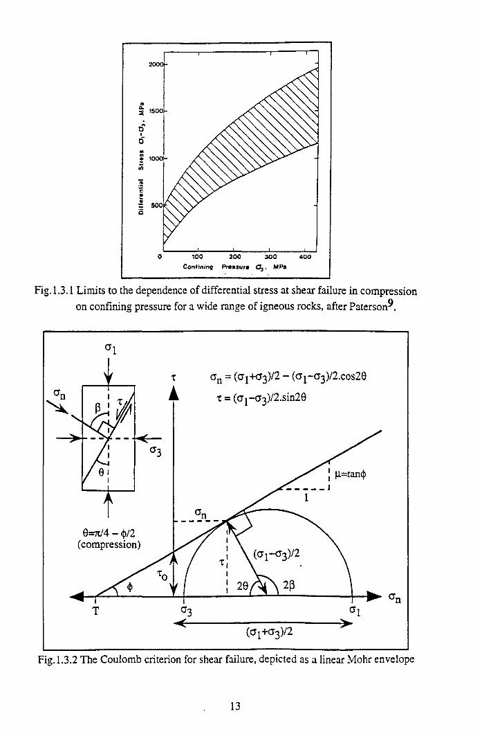
Fig. 1.3.1 Limits to the dependence of differential stress at shear failure in compression on confining pressure for a wide range of igneous rocks, after Paterson^.

Fig. 1.3.2 The Coulomb criterion for shear failure, depicted as a linear Mohr envelope

13

In this simple 2-D case, the intermediate principal stress, G2 (which is assumed to act

parallel to the strike of the shear plane and at right-angles to the direction of shear) has, in

theory, no influence upon failure. Whilst there are many methods of representing the

variation of stress in 2-D that of the Mohr circle diagram is by far the most important and

widely used (Mohr, 19007, 191410). Using this method, particular combinations of c i and

CT3 giving rise to shear failure are represented as Mohr circles in crn versus t stress-space.

The curve which is tangent to a series of such Mohr circles represents the failure

conditions for that material under test. Thus, a linear relationship between principal

stresses at failure, if represented by a series of Mohr circles, will exhibit a linear shear

failure envelope with the equation of the Coulomb criterion (Eqn. 1.3.3) as shown in

Fig. 1.3.2. From this construction it follows that:

(Gi - <J3)/2 = [(ai + aj)/2 + T0(l/tan<j>)]sin<j) ......... Eqn. 1.3.6

Eqn.1.3.6 can be rearranged to fit the linear form of Eqn.1.3.3:

G 1 = [(2t0cos<|>)/( 1 - sin<J)) + 03 {( 1 + sino)/( 1 - sin<)>)} ] ........ Eqn. 1.3.7

Hence, from Eqn. 1.3.7 it is apparent that the Coulomb criterion satisfies triaxial

compression data for rock types with a linear relationship between principal stresses at

failure. Further, from Eqn. 1.3.7 it follows that:

k = ( 1 + sin<»/( 1 - sin(j)) .......... Eqn. 1.3.8

G0 = 2x0.kAl/2 ........... Eqn. 1.3.9

Interestingly, the uniaxial compressive strength is related to both the cohesion and the

angle of internal friction. An important feature of the Coulomb criterion is that the angle

14

0 between the shear fracture plane and the axis of the maximum principal stress (9 =

faultA<Ji) can be predicted. To do this it is necessary to express the failure criterion as

given in Eqn. 1.3.4 in terms of the principal stresses, as depicted graphically in Fig. 1.3.2.

This expression is then differentiated with respect to 0 and the optimum conditions for

shear failure obtained. It can be shown that for optimum shear conditions:

+0 = (45° - <)>/2) ... ...... Eqn. 1.3.10

20 = 90° - <j) ...... ... Eqn.1.3.11

In Eqn. 1.3.11 (minus sign for compression, plus sign for tension) 20 is the acute angle

between conjugate shear planes. This angle is represented graphically by the acute angle a

tangent line to the linear envelope makes with the normal stress axis. A shortcoming of

the Coulomb criterion lies in its prediction o f the magnitude of the tensile strength, T,

which from Fig. 1.3.2 is:

T = to/tan<|) .......... Eqn.1.3.12

For angles of (><45°, that is for most sedimentary rocks, it follows that the predicted

tensile strength is greater than the cohesive strength, however this prediction is at

variance with empirical experience which frequently shows tensile strength to be around

half the magnitude of the cohesion.

Jaegar & Cook (page 425) note that, "all the phenomena of brittle fracture studied.... on a

laboratory scale appear to be reproduced on a geological scale. Faults are geological

fractures of rock in which there is relative displacement in the plane of fracture. They are

thus shear fractures.....and Griggs and Handin I960)11 and others have used the term

"fault" for shear fractures both on the laboratory and geological scale." Geological

faulting was discussed by Anderson (1951)12 on the basis of the Coulomb and Mohr

theories of shear fracture and classified according to the relative magnitudes of the

15

principal stresses, C7 1x 7 2 x 73 . Anderson based his classification on the general

observation that in many areas of the world, especially in those of low topographic relief,

it an be inferred from studies of joints, faults and dykes, that the axes of principal stress

are close to the horizontal or vertical. Anderson postulated a "standard state" of stress in

the Earth's crust, equivalent to a hydrostatic state in that the magnitudes of the horizontal

stresses at any specific depth in the crust, are equal to that o f the vertical geostatic stress

induced at that depth by gravitational loading. Based on the Coulomb and Mohr theories,

fracture takes place in one or both of a pair of conjugate planes which pass through the

direction of <72 and are equally inclined at angles <45° to the direction of <7 i. Since the

surface of the earth is a free surface, one of the principal stresses at the surface must be

normal to it, so it is reasonable to assume that one principal stress is vertical at moderate

depths. Anderson postulated that the magnitudes of the horizontal stresses, relative to that

of the vertical geostatic stress, could change in one o f three ways and (if the changes in

the magnitudes of the stresses were sufficient) could result in fault formation. The three

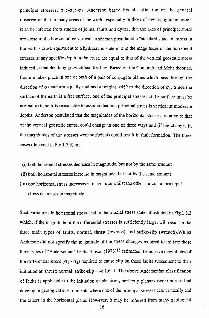
cases (depicted in Fig. 1.3.3) are:

(i) both horizontal stresses decrease in magnitude, but not by the same amount

(ii) both horizontal stresses increase in magnitude, but not by the same amount

(iii) one horizontal stress increases in magnitude whilst the other horizontal principal

stress decreases in magnitude

Such variations in horizontal stress lead to the triaxial stress states illustrated in Fig.1.3.3

which, if the magnitude of the differential stresses is sufficiently large, will result in the

three main types of faults, normal, thrust (reverse) and strike-slip (wrench).Whilst

Anderson did not specify the magnitude of the stress changes required to initiate these

three types of "Andersonian" faults, Sibson (1973)13 estimated the relative magnitudes of

the differential stress (<7i - <73) required to cause slip on these faults subsequent to their

initiation at: thrust: normal: strike-slip = 4: 1.6: 1. The above Andersonian classification

of faults is applicable to the initiation of idealised, perfectly planar discontinuities that

develop in geological environments where one of the principal stresses acts vertically and

the others in the horizontal plane. However, it may be inferred from many geological16

Fig. 1.3.3 Andersonian fault classification showing the three possible ways in which the"standard state" (SS) may be varied, producing the three corresponding fault-types-normal, thrust (reverse) and strike-slip, after Price & C osgrove^.

structures that the axes of principal stress are inclined away from the vertical and

horizontal (for example asymmetric folds imply an axis of principal compression inclined

to the horizontal).

Broadly speaking, two different approaches have been taken in the development of a

theory of brittle failure to predict macroscopic fracture stress. The first, empirical

approach advocates criteria of failure consistent with observed failure conditions under

particular experimental configurations but whose applicability is intended to extend to

more general stress states. The Coulomb and Mohr criteria are thus failure theories in this

sense. Although they are discussed in physical terms such as limits on stresses on

particular planes, they do not attempt to address the physical mechanisms of failure and

are therefore best regarded as empirical. Their main role is to provide a basis for

calculating failure conditions in practical situations. The second approach attempts to

build up physical models of brittle fracture which are amenable to theoretical treatment,

so that, whilst a degree of empiricism is still involved, the models aim to contribute to the

physical understanding of the fracture process. The Griffith theory, and those approaches

based on it, are the best-known in this second group.

An excellent overview of the Griffith-type theories of brittle failure can be found in

Paterson9, pages51-70. One of the most significant advances in the theory of fracture was

the proposal made by Griffith in 192014 that the strength of brittle materials is governed

by the initial presence of small cracks or "flaws". To calculate the tensile strength,

Griffith introduced an approach which in effect uses surface energy as a measure of the

local cohesive strength of the material. This failure criterion, based on the principle that

the potential energy of a system will tend to a minimum, is that the crack will propagate

if in doing so the sum of the following three terms is zero or negative:

(i) the surface energy of the newly created crack

(ii) the change in the elastic strain energy of the body

(iii) the change in the potential energy of the loading system

18

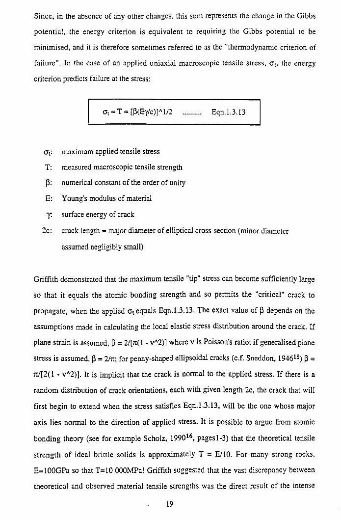
Since, in the absence of any other changes, this sum represents the change in the Gibbs

potential, the energy criterion is equivalent to requiring the Gibbs potential to be

minimised, and it is therefore sometimes referred to as the "thermodynamic criterion of

failure". In the case of an applied uniaxial macroscopic tensile stress, c t, the energy

criterion predicts failure at the stress:

a t = T = [p(Eyc)]Al /2 .......... Eqn.1.3.13

a t: maximum applied tensile stress

T: measured macroscopic tensile strength

P: numerical constant of the order of unity

E: Young's modulus of material

j . surface energy of crack

2 c: crack length = major diameter of elliptical cross-section (minor diameter

assumed negligibly small)

Griffith demonstrated that the maximum tensile "tip" stress can become sufficiently large

so that it equals the atomic bonding strength and so permits the "critical" crack to

propagate, when the applied Ct equals Eqn.1.3.13. The exact value of p depends on the

assumptions made in calculating the local elastic stress distribution around the crack. If

plane strain is assumed, P = 2/[m( 1 - vA2 )] where v is Poisson’s ratio; if generalised plane

stress is assumed, P = 2 /tc; for penny-shaped ellipsoidal cracks (c.f. Sneddon, 194615) p =

:t/[2 (l - v A2)J. It is implicit that the crack is normal to the applied stress. If there is a

random distribution of crack orientations, each with given length 2 c, the crack that will

first begin to extend when the stress satisfies Eqn.1.3.13, will be the one whose major

axis lies normal to the direction of applied stress. It is possible to argue from atomic

bonding theory (see for example Scholz, 199016, pages 1-3) that the theoretical tensile

strength of ideal brittle solids is approximately T = E/10. For many strong rocks,

E=100GPa so that T=10 OOOMPa! Griffith suggested that the vast discrepancy between

theoretical and observed material tensile strengths was the direct result of the intense

19

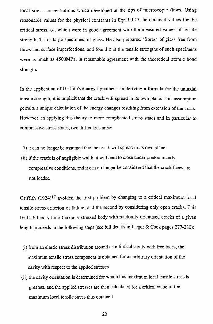
local stress concentrations which developed at the tips of microscopic flaws. Using

reasonable values for the physical constants in Eqn. 1.3.13, he obtained values for the

critical stress, a t, which were in good agreement with the measured values of tensile

strength, T, for large specimens of glass. He also prepared "fibres" of glass free from

flaws and surface imperfections, and found that the tensile strengths of such specimens

were as much as 4500MPa, in reasonable agreement with the theoretical atomic bond

strength.

In the application of Griffith's energy hypothesis in deriving a formula for the uniaxial

tensile strength, it is implicit that the crack will spread in its own plane. This assumption

permits a unique calculation of the energy changes resulting from extension o f the crack.

However, in applying this theory to more complicated stress states and in particular to

compressive stress states, two difficulties arise:

(i) it can no longer be assumed that the crack will spread in its own plane

(ii) if the crack is of negligible width, it will tend to close under predominantly

compressive conditions, and it can no longer be considered that the crack faces are

not loaded

Griffith (1924)17 avoided the first problem by changing to a critical maximum local

tensile stress criterion of failure, and the second by considering only open cracks. This

Griffith theory for a biaxially stressed body with randomly orientated cracks of a given

length proceeds in the following steps (see full details in Jaeger & Cook pages 277-280):

(i) from an elastic stress distribution around an elliptical cavity with free faces, the

maximum tensile stress component is obtained for an arbitrary orientation of the

cavity with respect to the applied stresses

(ii) the cavity orientation is determined for which this maximum local tensile stress is

greatest, and the applied stresses are then calculated for a critical value of the

maximum local tensile stress thus obtained

20

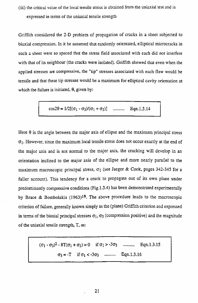
(iii) the critical value of the local tensile stress is obtained from the uniaxial test and is

expressed in terms of the uniaxial tensile strength

Griffith considered the 2-D problem of propagation of cracks in a sheet subjected to

biaxial compression. In it he assumed that randomly orientated, elliptical microcracks in

such a sheet were so spaced that the stress field associated with each did not interfere

with that of its neighbour (the cracks were isolated). Griffith showed that even when the

applied stresses are compressive, the "tip" stresses associated with each flaw would be

tensile and that these tip stresses would be a maximum for elliptical cavity orientation at

which the failure is initiated, 0 , given by:

cos20 = l/2[(c?i - ri3)/(cri + C3)] .......... Eqn.1.3.14

Here 0 is the angle between the major axis of ellipse and the maximum principal stress

(Jl. However, since the maximum local tensile stress does not occur exactly at the end of

the major axis and is not normal to the major axis, the cracking will develop in an

orientation inclined to the major axis of the ellipse and more nearly parallel to the

maximum macroscopic principal stress, (Ji (see Jaeger & Cook, pages 342-345 for a

fuller account). This tendency for a crack to propagate out of its own plane under

predominantly compressive conditions (Fig. 1.3.4) has been demonstrated experimentally

by Brace & Bombolakis (1963)1**. The above procedure leads to the macroscopic

criterion of failure, generally known simply as the (plane) Griffith criterion and expressed

in terms of the biaxial principal stresses Gi, G3 (compression positive) and the magnitude

of the uniaxial tensile strength, T, as:

(C i - G3)2 - 8T(ai + G3) = 0 if G i > -3G3 ........... Eqn.1.3.15

G3 = -T i f c i < - 3 C 3 .......... Eqn.1.3.16

21

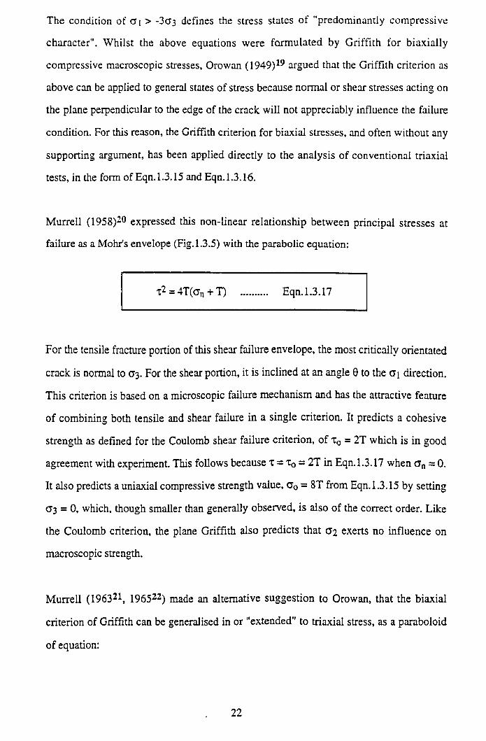
The condition of a t > -3a 3 defines the stress states of "predominantly compressive

character". Whilst the above equations were formulated by Griffith for biaxially

compressive macroscopic stresses, Orowan (1949)19 argued that the Griffith criterion as

above can be applied to general states of stress because normal or shear stresses acting on

the plane perpendicular to the edge of the crack will not appreciably influence the failure

condition. For this reason, the Griffith criterion for biaxial stresses, and often without any

supporting argument, has been applied directly to the analysis of conventional triaxial

tests, in the form of Eqn.1.3.15 and Eqn.1.3.16.

Murrell (1958)20 expressed this non-linear relationship between principal stresses at

failure as a Mohr's envelope (Fig. 1.3.5) with the parabolic equation:

x2 = 4T(an + T) .......... Eqn.1.3.17

For the tensile fracture portion of this shear failure envelope, the most critically orientated

crack is normal to (73. For the shear portion, it is inclined at an angle 0 to the a i direction.

This criterion is based on a microscopic failure mechanism and has the attractive feature

of combining both tensile and shear failure in a single criterion. It predicts a cohesive

strength as defined for the Coulomb shear failure criterion, of t 0 = 2T which is in good

agreement with experiment. This follows because x = x0 = 2T in Eqn.1.3.17 when Gn = 0.

It also predicts a uniaxial compressive strength value, G0 = 8T from Eqn.1.3.15 by setting

G3 = 0, which, though smaller than generally observed, is also of the correct order. Like

the Coulomb criterion, the plane Griffith also predicts that G2 exerts no influence on

macroscopic strength.

Murrell (196321, 196522) made an alternative suggestion to Orowan, that the biaxial

criterion of Griffith can be generalised in or "extended" to triaxial stress, as a paraboloid

of equation:

22

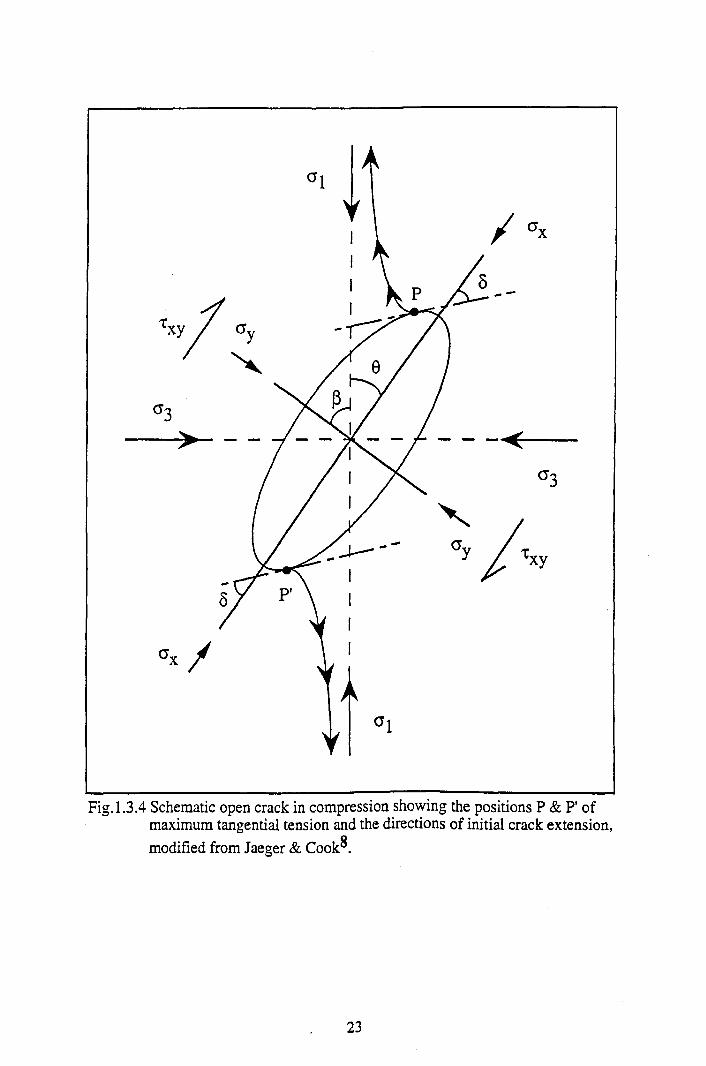
a l

Fig. 1.3.4 Schematic open crack in compression showing the positions P & F of maximum tangential tension and the directions of initial crack extension,modified from Jaeger & Cook^.

23

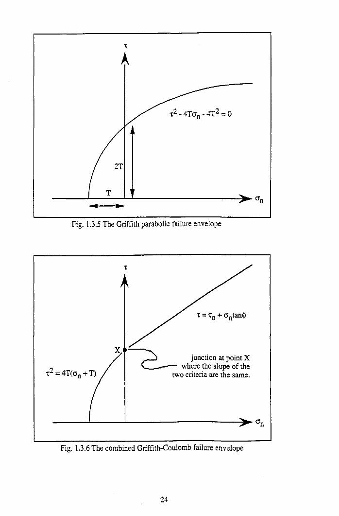
Fig. 1.3.6 The combined Griffith-Coulomb failure envelope

24

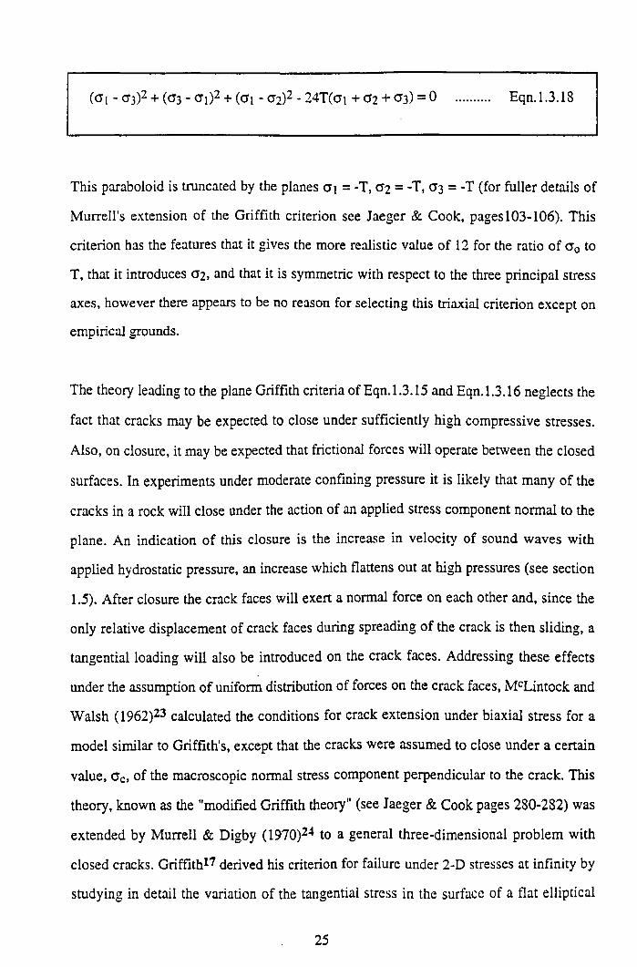
(G[ - C3)2 + (03 - cti)2 + (ai - <T2)2 - 24T(ai + 02 + <73) = 0 Eqn.1.3.18

This paraboloid is truncated by the planes Cti =-T, 02 = -T, 03 = -T (for fuller details of

Murrell's extension of the Griffith criterion see Jaeger & Cook, pages 103-106). This

criterion has the features that it gives the more realistic value of 12 for the ratio of o 0 to

T, that it introduces 0 2 , and that it is symmetric with respect to the three principal stress

axes, however there appears to be no reason for selecting this triaxial criterion except on

empirical grounds.

The theory leading to the plane Griffith criteria of Eqn.1.3.15 and Eqn.1.3.16 neglects the

fact that cracks may be expected to close under sufficiently high compressive stresses.

Also, on closure, it may be expected that frictional forces will operate between the closed

surfaces. In experiments under moderate confining pressure it is likely that many of the

cracks in a rock will close under the action of an applied stress component normal to the

plane. An indication of this closure is the increase in velocity of sound waves with

applied hydrostatic pressure, an increase which flattens out at high pressures (see section

1.5). After closure the crack faces will exert a normal force on each other and, since the

only relative displacement of crack faces during spreading of the crack is then sliding, a

tangential loading will also be introduced on the crack faces. Addressing these effects

under the assumption of uniform distribution of forces on the crack faces, McLintock and

W alsh (1962)23 calculated the conditions for crack extension under biaxial stress for a

model similar to Griffith's, except that the cracks were assumed to close under a certain

value, gc, of the macroscopic normal stress component perpendicular to the crack. This

theory, known as the "modified Griffith theory" (see Jaeger & Cook pages 280-282) was

extended by Murrell & Digby (1970)24 to a general three-dimensional problem with

closed cracks. Griffith17 derived his criterion for failure under 2-D stresses at infinity by

studying in detail the variation of the tangential stress in the surface of a flat elliptical

25

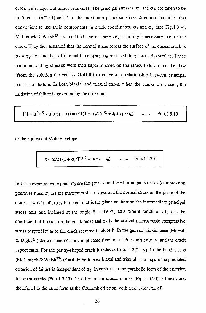
crack with major and minor semi-axes. The principal stresses, a [ and (J3, are taken to be

inclined at (tt/2 +P) and P to the maximum principal stress direction, but it is also

convenient to use their components in crack coordinates, a x and a y (see Fig. 1.3.4).

McLintock & Walsh23 assumed that a normal stress a c at infinity is necessary to close the

crack. They then assumed that the normal stress across the surface of the closed crack is

Gn = Gy - ac and that a frictional force Tf = ji.crn resists sliding across the surface. These

frictional sliding stresses were then superimposed on the stress field around the flaw

(from the solution derived by Griffith) to arrive at a relationship between principal

stresses at failure. In both biaxial and triaxial cases, when the cracks are closed, the

initiation of failure is governed by the criterion:

[(1 +p.2)1/2 - jj .] .(a i-C 3) = a 'T ( l + a c/T)1/2+ 2 ji(a3 - a c) .......... Eqn.1.3.19

or the equivalent Mohr envelope:

x = oc'/2T( 1 + Cc/T)1 /2+ ß(cn - o c) .......... Eqn. 1.3.20

In these expressions, Gi and 03 are the greatest and least principal stresses (compression

positive) x and crn are the maximum shear stress and the normal stress on the plane of the

crack at which failure is initiated, that is the plane containing the intermediate principal

stress axis and inclined at the angle 0 to the (?i axis where tan29 = l / |i , (i is the

coefficient of friction on the crack faces and oc is the critical macroscopic compressive

stress perpendicular to the crack required to close it. In the general triaxial case (Murrell

& Digby24) the constant a ' is a complicated function o f Poisson's ratio, v, and the crack

aspect ratio. For the penny-shaped crack it reduces to a ' = 2(2 - v). In the biaxial case

(McLintock & Walsh23) a ' = 4. In both these biaxal and triaxial cases, again the predicted

criterion of failure is independent of 0 2- In contrast to the parabolic form of the criterion

for open cracks (Eqn.1.3.17) the criterion for closed cracks (Eqn.1.3.20) is linear, and

therefore has the same form as the Coulomb criterion, with a cohesion, x0, of:

26

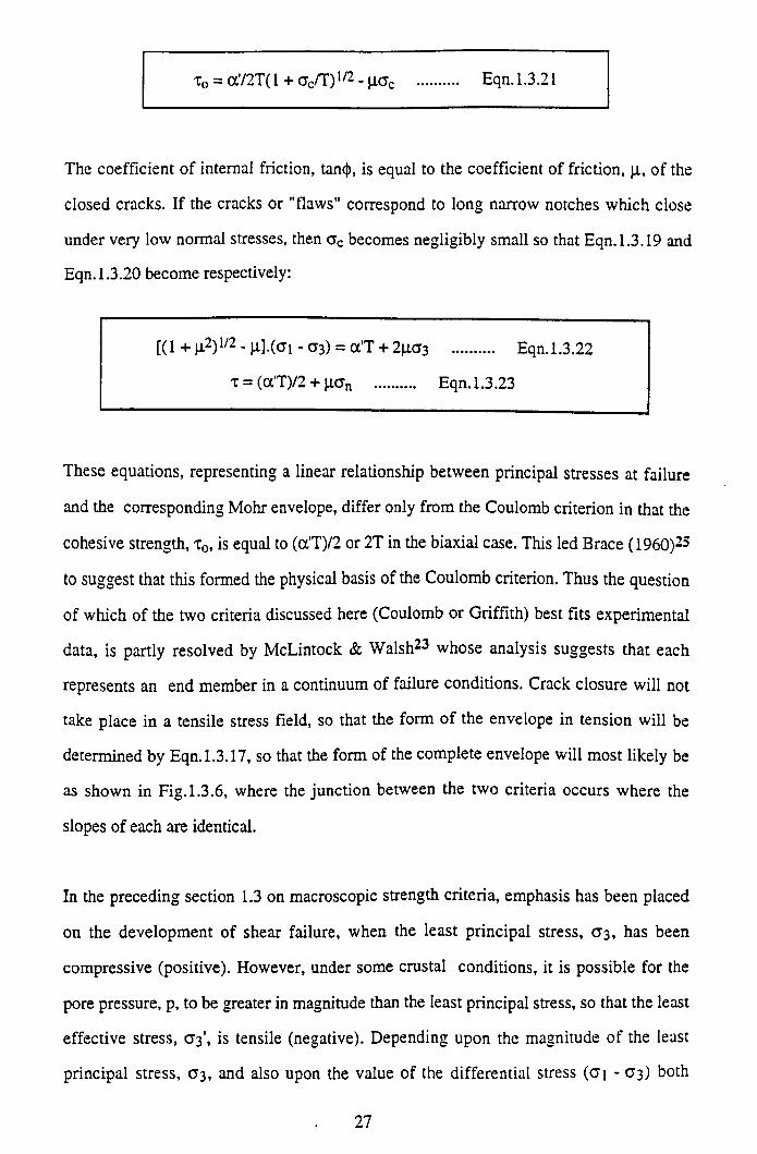
T o = cc'/2T(l + a c/T )1/2 - (iac Eqn. 1.3.21

The coefficient of internal friction, tan<J>, is equal to the coefficient of friction, fi, of the

closed cracks. If the cracks or "flaws" correspond to long narrow notches which close

under very low normal stresses, then a c becomes negligibly small so that Eqn. 1.3.19 and

Eqn. 1.3.20 become respectively:

[(1 + |i 2) 1/2 -^].(ci-C T3) = a 'T + 2^ a 3 .......... Eqn. 1.3.22

x = (a'T)/2 + p a n .......... Eqn. 1.3.23

These equations, representing a linear relationship between principal stresses at failure

and the corresponding Mohr envelope, differ only from the Coulomb criterion in that the

cohesive strength, t0, is equal to (a'T)/2 or 2T in the biaxial case. This led Brace (I960)25

to suggest that this formed the physical basis of the Coulomb criterion. Thus the question

of which of the two criteria discussed here (Coulomb or Griffith) best fits experimental

data, is partly resolved by McLintock & Walsh23 whose analysis suggests that each

represents an end member in a continuum of failure conditions. Crack closure will not

take place in a tensile stress field, so that the form of the envelope in tension will be

determined by Eqn.1.3.17, so that the form of the complete envelope will most likely be

as shown in Fig. 1.3.6, where the junction between the two criteria occurs where the

slopes of each are identical.

In the preceding section 1.3 on macroscopic strength criteria, emphasis has been placed

on the development of shear failure, when the least principal stress, g 3, has been

compressive (positive). However, under some crustal conditions, it is possible for the

pore pressure, p, to be greater in magnitude than the least principal stress, so that the least

effective stress, c 3', is tensile (negative). Depending upon the magnitude of the least

principal stress, c 3, and also upon the value of the differential stress (a i - a 3) both

27

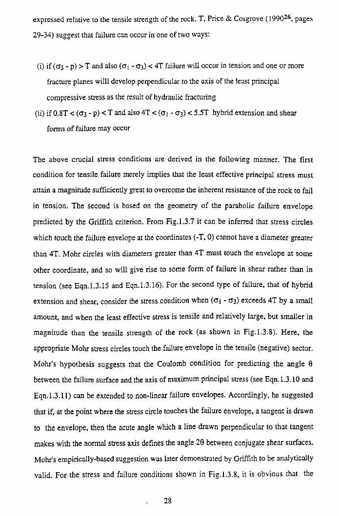
expressed relative to the tensile strength of the rock, T, Price & Cosgrove ( 199026, pages

29-34) suggest that failure can occur in one of two ways:

(i) if (G3 - p) > T and also (G[ - G3) < 4T failure will occur in tension and one or more

fracture planes willl develop perpendicular to the axis of the least principal

compressive stress as the result of hydraulic fracturing

(ii) if 0.8T < (03 - p) < T and also 4T < (a i - 0 3 ) < 5.5T hybrid extension and shear

forms of failure may occur

The above crucial stress conditions are derived in the following manner. The first

condition for tensile failure merely implies that the least effective principal stress must

attain a magnitude sufficiently great to overcome the inherent resistance of the rock to fail

in tension. The second is based on the geometry of the parabolic failure envelope

predicted by the Griffith criterion. From Fig. 1.3.7 it can be inferred that stress circles

which touch the failure envelope at the coordinates (-T, 0) cannot have a diameter greater

than 4T. Mohr circles with diameters greater than 4T must touch the envelope at some

other coordinate, and so will give rise to some form of failure in shear rather than in

tension (see Eqn.1.3.15 and Eqn.1.3.16). For the second type of failure, that of hybrid

extension and shear, consider the stress condition when (a i - CT3) exceeds 4T by a small

amount, and when the least effective stress is tensile and relatively large, but smaller in

magnitude than the tensile strength of the rock (as shown in Fig. 1.3.8). Here, the

appropriate Mohr stress circles touch the failure envelope in the tensile (negative) sector.

Mohr's hypothesis suggests that the Coulomb condition for predicting the angle 9

between the failure surface and the axis of maximum principal stress (see Eqn.1.3.10 and

Eqn.1.3.11) can be extended to non-linear failure envelopes. Accordingly, he suggested

that if, at the point where the stress circle touches the failure envelope, a tangent is drawn

to the envelope, then the acute angle which a line drawn perpendicular to that tangent

makes with the normal stress axis defines the angle 29 between conjugate shear surfaces.

Mohr's empirically-based suggestion was later demonstrated by Griffith to be analytically

valid. For the stress and failure conditions shown in Fig. 1.3.8, it is obvious that the

28

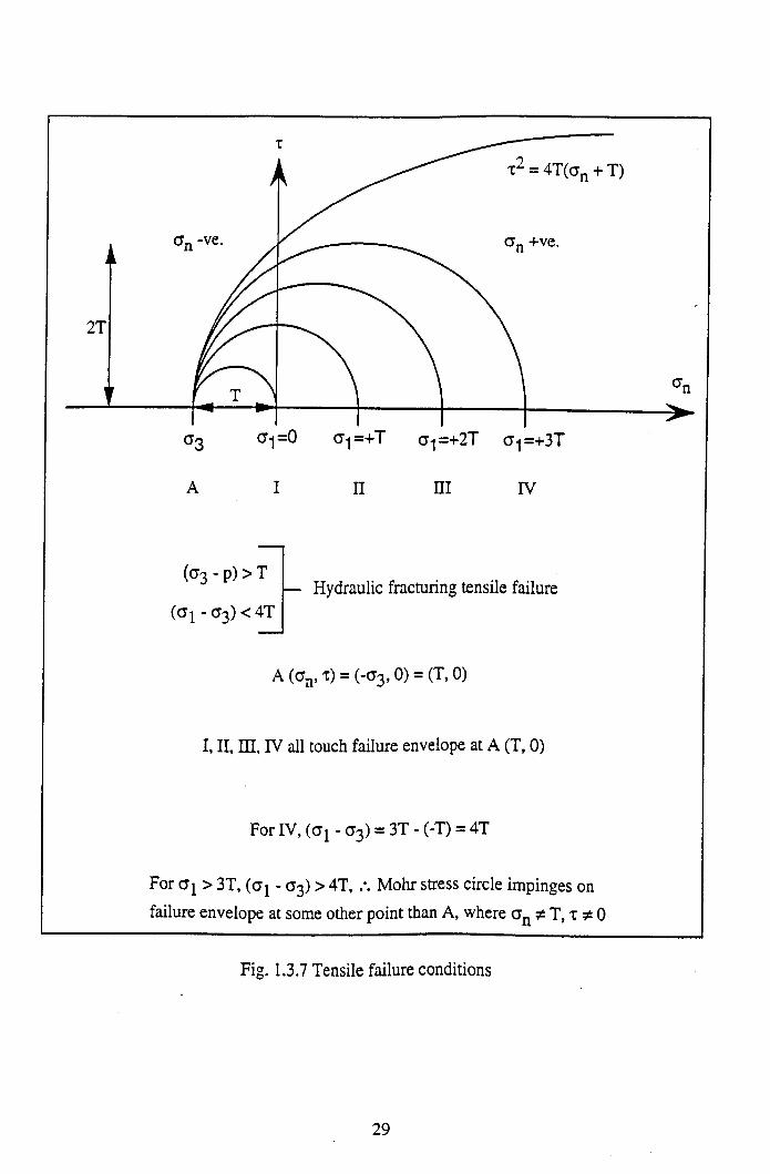
Fig. 1.3.7 Tensile failure conditions

29

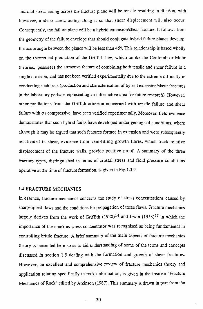
normal stress acting across the fracture plane will be tensile resulting in dilation, with

however, a shear stress acting along it so that shear displacement will also occur.

Consequently, the failure plane will be a hybrid extension/shear fracture. It follows from

the geometry of the failure envelope that should conjugate hybrid failure planes develop,

the acute angle between the planes will be less than 45°. This relationship is based wholly

on the theoretical prediction of the Griffith law, which unlike the Coulomb or Mohr

theories, possesses the attractive feature of combining both tensile and shear failure in a

single criterion, and has not been verified experimentally due to the extreme difficulty in

conducting such tests (production and characterisation of hybrid extension/shear fractures

in the laboratory perhaps representing an informative area for future research). However,

other predictions from the Griffith criterion concerned with tensile failure and shear

failure with as compressive, have been verified experimentally. Moreover, field evidence

demonstrates that such hybrid faults have developed under geological conditions, where

although it may be argued that such features formed in extension and were subsequently

reactivated in shear, evidence from vein-filling growth fibres, which track relative

displacement of the fracture walls, provide positive proof. A summary of the three

fracture types, distinguished in terms of crustal stress and fluid pressure conditions

operative at the time of fracture formation, is given in Fig. 1.3.9.

1.4 FRACTURE MECHANICS

In essence, fracture mechanics concerns the study of stress concentrations caused by

sharp-tipped flaws and the conditions for propagation of these flaws. Fracture mechanics

largely derives from the work of Griffith (1920)14 and Irwin (1958)27 in which the

importance of the crack as stress concentrator was recognised as being fundamental in

controlling brittle fracture. A brief summary of the main aspects of fracture mechanics

theory is presented here so as to aid understanding o f some of the terms and concepts

discussed in section 1.5 dealing with the formation and growth of shear fractures.

However, an excellent and comprehensive review of fracture mechanics theory and

application relating specifically to rock deformation, is given in the treatise "Fracture

Mechanics of Rock" edited by Atkinson (1987). This summary is drawn in part from the

30

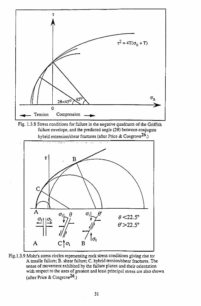
Fig. 1.3.8 Stress conditions for failure in the negative quadrants of the Griffith failure envelope, and the predicted angle (29) between conjugatehybrid extension/shear fractures (after Price & C osgrove^.)

Fig. 1.3.9 Mohr's stress circles representing rock stress conditions giving rise to:A tensile failure; B. shear failure; C. hybrid tension/shear fractures. The sense of movement exhibited by the failure planes and their orientation with respect to the axes of greatest and least principal stress are also shown(after Price & Cosgrove^.)

31

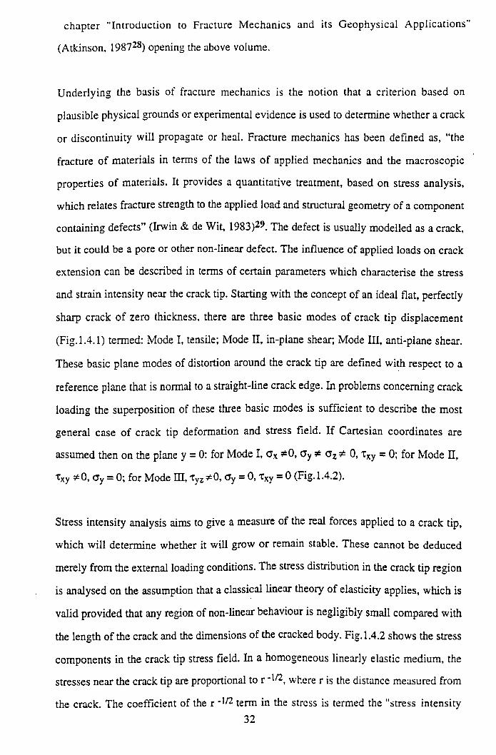
chapter "Introduction to Fracture Mechanics and its Geophysical Applications"

(Atkinson, 198728) opening the above volume.

Underlying the basis of fracture mechanics is the notion that a criterion based on

plausible physical grounds or experimental evidence is used to determine whether a crack

or discontinuity will propagate or heal. Fracture mechanics has been defined as, “the

fracture of materials in terms of the laws of applied mechanics and the macroscopic

properties of materials. It provides a quantitative treatment, based on stress analysis,

which relates fracture strength to the applied load and structural geometry of a component

containing defects” (Irwin & de Wit, 1983)29. The defect is usually modelled as a crack,

but it could be a pore or other non-linear defect. The influence of applied loads on crack

extension can be described in terms of certain parameters which characterise the stress

and strain intensity near the crack tip. Starting with the concept of an ideal flat, perfectly

sharp crack of zero thickness, there are three basic modes o f crack tip displacement

(Fig. 1.4.1) termed: Mode I, tensile; Mode II, in-plane shear; Mode HI, anti-plane shear.

These basic plane modes of distortion around the crack tip are defined with respect to a

reference plane that is normal to a straight-line crack edge. In problems concerning crack

loading the superposition of these three basic modes is sufficient to describe the most

general case of crack tip deformation and stress field. If Cartesian coordinates are

assumed then on the plane y = 0: for Mode I, Gx *0, Gy * 0, TXy = 0; for Mode n ,

Txy *0 , Gy = 0; for Mode EH, xyz *0, Gy = 0, Txy = 0 (Fig. 1.4.2).

Stress intensity analysis aims to give a measure of the real forces applied to a crack tip,

which will determine whether it will grow or remain stable. These cannot be deduced

merely from the external loading conditions. The stress distribution in the crack tip region

is analysed on the assumption that a classical linear theory of elasticity applies, which is

valid provided that any region of non-linear behaviour is negligibly small compared with

the length of the crack and the dimensions of the cracked body. Fig. 1.4.2 shows the stress

components in the crack tip stress field. In a homogeneous linearly elastic medium, the

stresses near the crack tip are proportional to r *1/2, where r is the distance measured from

the crack. The coefficient of the r _1/2 term in the stress is termed the "stress intensity32

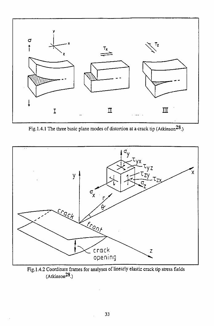
Fig. 1.4.1 The three basic plane modes of distortion at a crack tip (A tkinson^.)

Fig. 1.4.2 Coordinate frames for analyses of linearly elastic crack tip stress fields(A tkinson^.)

33

factor" and it depends on such factors as the applied load, the shape of the body and the

crack length. The stress intensity factor, K, is thus the magnitude of the crack tip stress

field for a particular mode in a homogeneous linear elastic material. As a simple

demonstration, for the values of the c yy stress component in Mode I at points near the

crack tip within the material in the plane of the crack, the elastic solution is:

a yy = a.(c/2r) 172 ..... Eqn. 1.4.1

2 c: crack length,

r: distance from the crack tip.

a : macroscopic stress applied normal to the crack.

(Eqn. 1.4.1) can be written in the form:

Cyy = K\/ (2m)m ..... Eqn. 1.4.2

Ki: a .(7tc )172.

The factor 1/(2rcr) 172 is the distribution function along the r-axis and Ki = c.(jtc ) 172

is the scaling factor or stress intensity factor. Full expressions for all the components of

stress and displacement at all points in the reference plane in each of the three basic

modes of distortion can be found in the extensive literature. The dimensions of K are

stress x (crack length)172, that is Pa* (m) 172 or N/m1-5.

Thus, for a particular loading on a specimen of particular shape, the mechanical situation

around a crack tip can be described in terms of stress intensity factors and the basic

distortion modes. With regard to what aspect of this local situation around the crack tip

determines when the crack will begin to spread under the action of increasing the external

loading, the simplest view is that the crack will begin to spread when a certain critical

34

intensity of loading is reached at its tip, as measured by the stress intensity factors. That

is, the failure criterion is expressed in terms of "critical stress intensity factors". These

factors are material parameters, depending on the type of material, its particular physical

condition of grain-size, strain-hardening etc. and the conditions of temperature and

pressure. They are designated Kic, Kjic and Kmc- When K reaches Kc, catastrophic

crack growth is assumed to occur. The material property Kjc is also called the "plane

strain fracture toughness". Practical procedures for determining the critical Kc parameters

for various materials have been extensively developed and codified (see ISRM

“Suggested Methods for Determining The Fracture Toughness o f Rock”, 198830).

Instead of considering crack tip stresses, an alternative fracture mechanics approach to

crack extension is to examine the "crack extension force" or "strain energy release rate",

G, which is the loss of energy per unit of new crack separation area formed during an

increment of crack extension. Note that G is a rate with respect to crack length and not

with respect to time. For fracture in each of the three fundamental modes of crack tip

displacement, the crack extension force for plane strain and assuming linear elasticity is

given by:

Gi - K i2(1-v2)/E .... Eqn. 1.4.3

Gn = Kn2(l-v 2)/E .... Eqn. 1.4.4

Gm = Kni2/2(i = Km2(l+v)/E ..... Eqn. 1.4.5

v: Poisson’s ratio.

E: Young’s modulus.

|i: Shear modulus.

For plane stress, the factor (1-v2) in Eqn.'s 1.4.3, 1.4.4 andl.4.5 is replaced by unity.

35

Thus a key concept in the widespread use of fracture mechanics is that extension of a

fracture will occur once a critical value of stress intensity factor, Kc, or crack extension

force, Gc» has been reached or exceeded. Once Kc or G c has been reached, crack

propagation is known as "fast/catastrophic fracture" because its speed can approach that

of sound in the medium, provided that the crack is isolated and its walls are traction free.

Classical fracture mechanics deals with a single, ideal atomically sharp crack. This is a

suitable representation for single crystals or at a microscopic level in polycrystalline

materials, extensive electron optical studies supporting the assertion that brittle cracks in

such materials are in fact atomically sharp and do propagate by the sequential rupturing

of bonds. However, at a more macroscopic level of study, real polycrystalline polyphase

materials such as rocks and ceramics show more complex behaviour. For sequential

loading of a blunt machined notch in rock, initially a few microcracks will form, but the

system behaviour will remain linear. On further loading, microcracking intensity will

increase, and behaviour in the crack tip region will become non-linear. Finally,

macrocrack extension will occur due to microcrack linkage in this non-linear zone,

known as the "process zone". The macrocrack propagates by taking with it a "damage

cloud" contained in the process zone. In some materials the process zone may be small

with respect to the dimensions of the cracked body and hence a fracture mechanics

analysis assuming linear elasticity (linear elastic fracture mechanics, LEFM) will still be

valid. However, if the process zone size becomes large, then non-linear fracture

mechanics analyses are required, such as the "J-integral" (for details of the J-integral and

its application to problems involving shear cracks in geophysics such as faults and

earthquakes, see Li, 198731). In fracture mechanics literature, the term process zone is

often given a more general meaning encompassing any zone of non-linear behaviour at a

crack tip, where for example plasticity as opposed to microcracking could be the means

by which the non-linearity is obtained.

For decades engineers have successfully used the critical stress intensity factor/critical

strain energy release rate approach to predict catastrophic crack propagation in metals,

ceramics, glasses and rocks. However, in systems subjected to long-term loading, this

36

classical approach breaks down, especially if high temperatures or reactive environments

are present. This is because significant rates of crack extension can occur at values of K,

G that may be substantially lower than K c, Gc- This phenomenon is known as

"subcritical crack growth". It was first observed in glass, but has subsequently been

observed in experiments on most engineering materials including rocks and minerals.

Subcritical crack growth can be due to several competing mechanisms, of which the most

familiar is "stress corrosion" or "hydrolytic weakening". A particular mechanism will be

dominant under specific ranges of environmental and material variables, hence as the

range of these variables in the earth’s crust is enormous, it might be expected that

different mechanisms will contribute to subcritical crack growth in different parts of the

crust and in the same part at different times. Stress corrosion crack growth occurs because

the chemical action of an environmental agent, such as water, weakens the strained bonds

at crack tips and so facilitates crack propagation. It occurs at crack velocities which

decrease as K is lowered to some threshold value Ko, below which no crack propagation

is observed. Well-known trimodal behaviour for subcritical crack growth studies on glass,

shows three distinct regions on a stress intensity factor versus crack velocity diagram, for

tensile crack growth by stress corrosion (see Fig. 1.2.3):

Region 1: crack growth velocity controlled by rate of stress corrosion reactions at

crack tips.

Region 2 : crack growth velocity controlled by the rate of transport of reactive

species to crack tips.

Region 3: crack growth mainly controlled by mechanical rupture, being relatively

insensitive to the chemical environment.

K o marks the lower bound to Region 1 whilst Kic marks the upper bound to Region 3.

1.5 EXPERIM ENTAL STUDIES OF SHEAR FAULTING

Santarelli and Brown (1989)32 in a study of the formation and propagation of surfaces of

discontinuity in rocks (brittle failure) to examine the possibility of predicting the

behaviour of rocks around model underground excavations, compiled a summary table of

37

experimental studies on the localisation of shear deformation (Table 1.5.1). As shown in

this table, several indirect techniques have been used to study the onset of localisation. A

large number of strain gauges bonded to a specimen can measure detailed surface

deformations, although the glue used could be construed as being disruptive to such

studies, therefore optical methods such as slit diffractometry are preferred. The most

common of these is holographic interferometry which allows the compilation of complete

surface strain maps and has been employed in uniaxial, biaxial and triaxial

experimentation. Sonic techniques have also been used, including both passive and active

microseismics. Acoustic emission monitoring records the high frequency elastic

vibrations emitted by propagating microcracks under deformation, with source location

via acoustic tomography providing important information on their location. Active

microseismics measures the velocity and attenuation of artificially transmitted elastic

waves (compressional “P-waves” and/or shear “S-waves”) which are highly sensitive to

the presence of cracks. Direct microscopic observation requires that specimens are

deformed stably through the post-failure region under servo-controlled displacement

control, to achieve stable crack propagation. For optical examination, samples may be

injected with a dyed resin prior to specimen unloading and sample thin-sectioning.

Alternatively electron microscopy has been used to study the sizes, shapes, orientations

and distribution/localisation of microcracks. From Table 1.5.1 it is evident that pre­

failure localisation of strain occurs at a hardening stage prior to peak strength,

Clocalisation/tfpeak varying from 60 to 99% for the rock types considered. Lithology

dependency aside, scatter in localisation ratios are partly the result of sensitivity to the

various measuring techniques employed, and the fact that early localisation can be

produced by poor specimen end-preparation.

Whilst Table 1.5.1 and the above microstructural observations refer primarily to igneous

rock types with their characteristic interlocking crystalline textures, Hallbauer, Wagner

and Cook (1973)33 performed triaxial compression tests on specimens of a fine-grained

argillaceous quartzite. Careful macroscopic and microscopic studies were conducted on

longitudinal sections from different specimens stopped at predetermined points along the

38

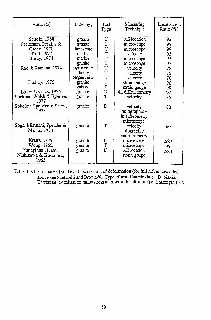
Author(s) Lithology TestType

MeasuringTechnique

Localisation Ratio (%)

Scholz, 1968 granite U AE location 92Freidman, Perkins & granite U microscope 99

Green, 1970 limestone U microscope 99Thill, 1972 marble T velocity 95

Brady, 1974 marble T microscope 95

Rao & Ramana, 1974granite T microscope 95

pyroxenite U velocity 78dunite U velocity 75

serpentinite U velocity 76Hadley, 1975 granite T strain gauge 90

gabbro T strain gauge 90Liu & Livanos, 1976 granite U slit diffractometry 92

Lockner, Walsh & Byerlee, 1977

granite T velocity 85

Sobolev, Spetzler & Salov, 1978

granite B velocity holographic - interferometry

microscope

80

Soga, Mizutani, Spetzler & Martin, 1978

granite T velocity holographic - interferometry

60

Kranz, 1979 granite U microscope >87Wong, 1982 granite T microscope 99

Yanagidani, Ehara, Nishizawa & Kusonose,

1985

granite U AE location strain gauge

>83

Table 1.5.1 Summary of studies of localisation of deformation (for full references cited above see Santarelli and Brown32). Type of test: U=uniaxial; B=biaxial; T=triaxial. Localisation ratio=stress at onset of localisation/peak strength (%).

39

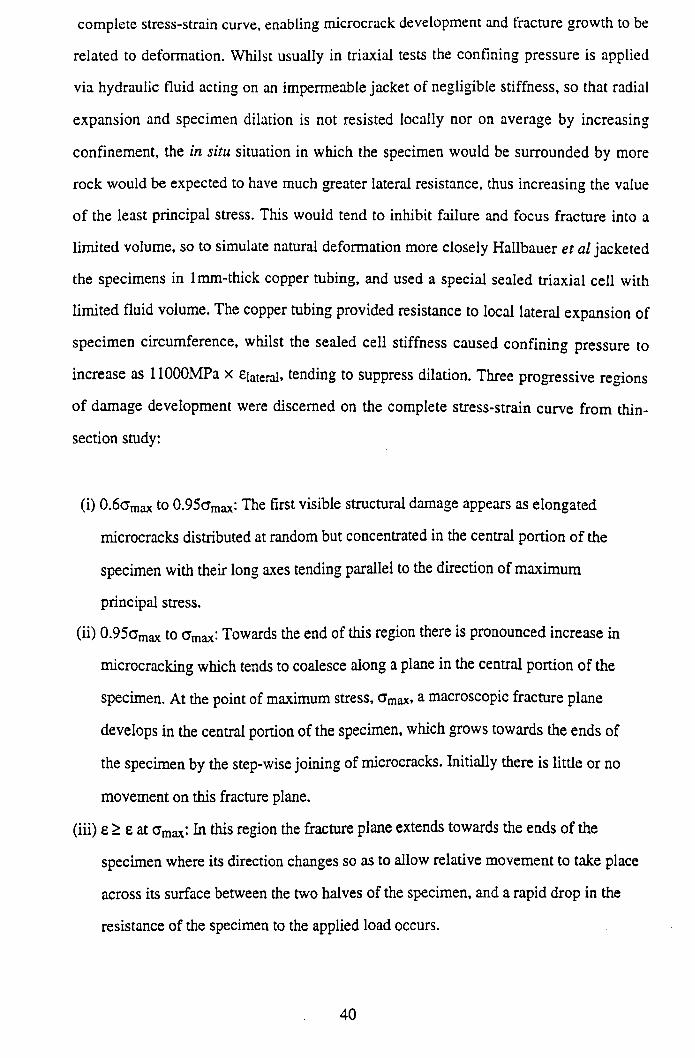
complete stress-strain curve, enabling microcrack development and fracture growth to be

related to deformation. Whilst usually in triaxial tests the confining pressure is applied

via hydraulic fluid acting on an impermeable jacket of negligible stiffness, so that radial

expansion and specimen dilation is not resisted locally nor on average by increasing

confinement, the in situ situation in which the specimen would be surrounded by more

rock would be expected to have much greater lateral resistance, thus increasing the value

o f the least principal stress. This would tend to inhibit failure and focus fracture into a

limited volume, so to simulate natural deformation more closely Hallbauer et al jacketed

the specimens in lmm-thick copper tubing, and used a special sealed triaxial cell with

limited fluid volume. The copper tubing provided resistance to local lateral expansion of

specimen circumference, whilst the sealed cell stiffness caused confining pressure to

increase as llOOOMPa x enteral, tending to suppress dilation. Three progressive regions

o f damage development were discerned on the complete stress-strain curve from thin-

section study:

(i) 0 .6amax to 0.95crmax: The first visible structural damage appears as elongated

microcracks distributed at random but concentrated in the central portion o f the

specimen with their long axes tending parallel to the direction of maximum

principal stress.

(ii) 0.95amax to a max: Towards the end of this region there is pronounced increase in

microcracking which tends to coalesce along a plane in the central portion of the

specimen. At the point of maximum stress, a max> a macroscopic fracture plane

develops in the central portion of the specimen, which grows towards the ends of

the specimen by the step-wise joining of microcracks. Initially there is little or no

movement on this fracture plane.

(iii) e > e at a max; hi this region the fracture plane extends towards the ends of the

specimen where its direction changes so as to allow relative movement to take place

across its surface between the two halves of the specimen, and a rapid drop in the

resistance of the specimen to the applied load occurs.

40

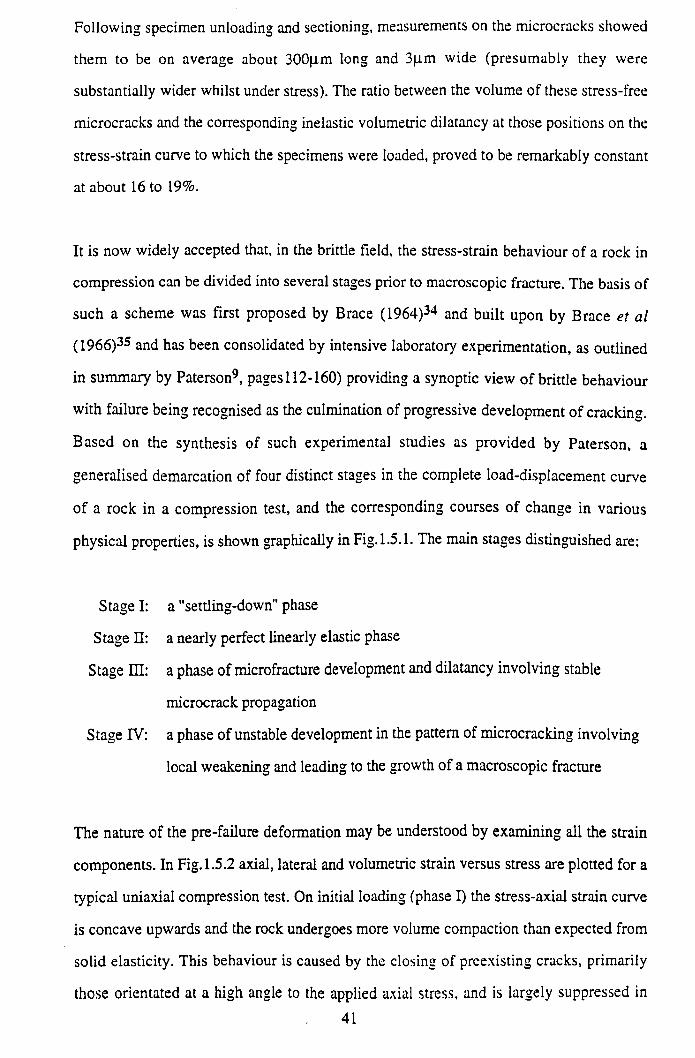
Following specimen unloading and sectioning, measurements on the microcracks showed

them to be on average about 300p.m long and 3|im wide (presumably they were

substantially wider whilst under stress). The ratio between the volume of these stress-free

microcracks and the corresponding inelastic volumetric dilatancy at those positions on the

stress-strain curve to which the specimens were loaded, proved to be remarkably constant

at about 16 to 19%.

It is now widely accepted that, in the brittle field, the stress-strain behaviour of a rock in

compression can be divided into several stages prior to macroscopic fracture. The basis of

such a scheme was first proposed by Brace (1964)34 and built upon by Brace et al

(1966)35 and has been consolidated by intensive laboratory experimentation, as outlined

in summary by Paterson9, pages 112-160) providing a synoptic view of brittle behaviour

with failure being recognised as the culmination of progressive development of cracking.

Based on the synthesis of such experimental studies as provided by Paterson, a

generalised demarcation of four distinct stages in the complete load-displacement curve

of a rock in a compression test, and the corresponding courses of change in various

physical properties, is shown graphically in Fig. 1.5.1. The main stages distinguished are:

Stage I: a "settling-down" phase

Stage II: a nearly perfect linearly elastic phase

Stage EH: a phase of microfracture development and dilatancy involving stable

microcrack propagation

Stage IV: a phase of unstable development in the pattern of microcracking involving

local weakening and leading to the growth of a macroscopic fracture

The nature of the pre-failure deformation may be understood by examining all the strain

components. In Fig. 1.5.2 axial, lateral and volumetric strain versus stress are plotted for a

typical uniaxial compression test. On initial loading (phase I) the stress-axial strain curve

is concave upwards and the rock undergoes more volume compaction than expected from

solid elasticity. This behaviour is caused by the closing of preexisting cracks, primarily

those orientated at a high angle to the applied axial stress, and is largely suppressed in

41

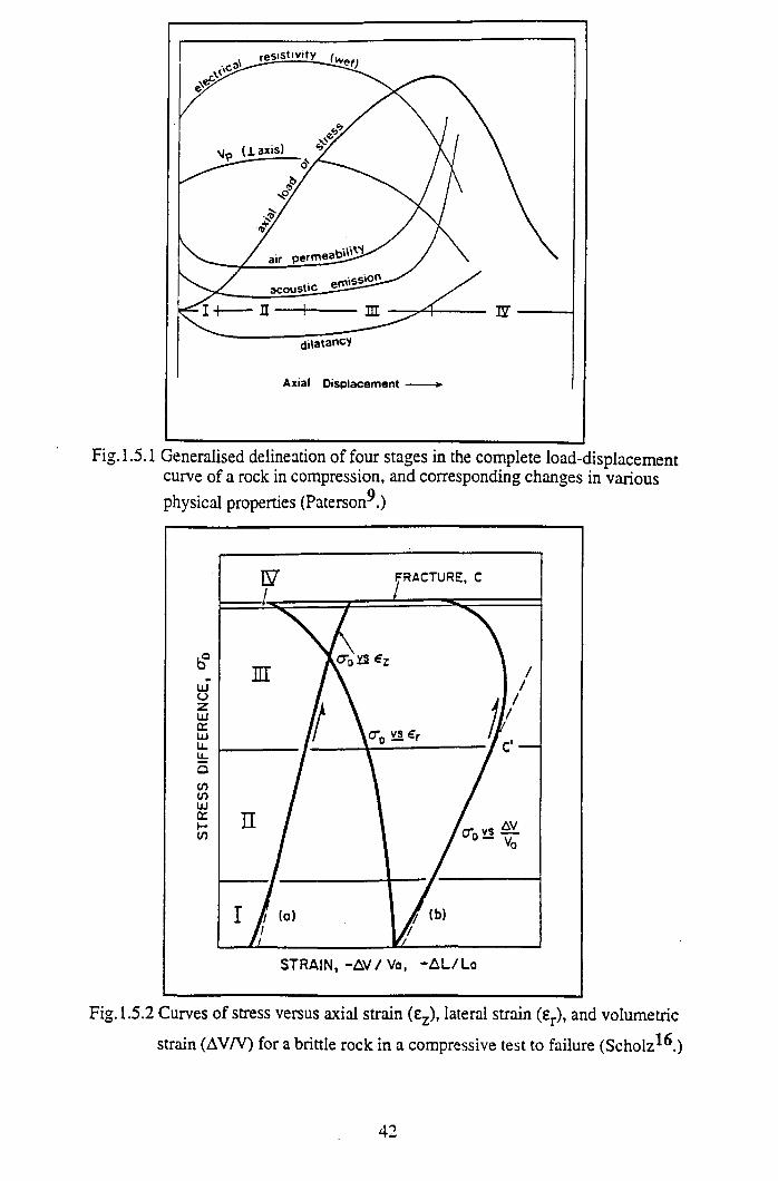
Fig. 1.5.1 Generalised delineation of four stages in the complete load-displacement curve of a rock in compression, and corresponding changes in variousphysical properties (Paterson^.)

Fig. 1.5.2 Curves of stress versus axial strain (ez), lateral strain (er), and volumetric

strain (AV/V) for a brittle rock in a compressive test to failure (S cholz^ .)

42

triaxial compression tests (although it does occur in tests performed under relatively low

confinement) as the confining pressure closes such cracks prior to application of a

deviatoric stress. This process is observed to be more or less completely reversible, that is

non-linearly elastic in its macroscopic effect. In more porous rocks, irreversible pore

collapse may also be expected to contribute in this stage, especially in uniaxial

compression, however this effect will not be restricted to stage I. After such cracks

orientated at a high angle to the maximum principal compressive stress have largely

closed, the rock deforms in a nearly linear elastic manner, according to its intrinsic elastic

constants (phase II). This stage is thought to involve predominantly the elastic

deformation of both constituent grains and pore space, however acoustic emission and

hysteresis detected in this stage indicates that some irreversible processes are occurring.

Some sliding on pre-existing cracks has been suggested (Bieniawski, 196736) relating the

shape of the hysteresis loop to the frictional resistance to such sliding, with reference to

the theory of Walsh (1965)37 however microscopical studies have failed to provide

evidence of shear crack activity, so that the explanation for hysteresis must remain

somewhat conjectural although whatever is occurring is probably premonitory to the

developments in stage in. The sensitivity with which non-linearity in the stress-strain

curve can be detected of course influences the extent attributed to stage II, but it is

evident that this extent also varies considerably with rock type and confining pressure. At

an axial stress magnitude commonly found to be around half the peak failure stress, the

rock specimen is observed to dilate relative to what would be expected from linear

elasticity (stage El). This dilation is accompanied by a decrease in the axial modulus, but

is primarily due to nonelastic lateral expansion (Fig. 1.5.2).

This rheological property in which volume dilation occurs as a result of application of a

deviatoric stress, is known as dilatancy. Prior to the work of Brace et a l35 dilatancy was

known primarily only as a property of granular material, however, following their work,

it can be interpreted with regard to rock material, as resulting from the development of

pervasive microcracking within the rock with a concomitant increase in void space. The

AE that occurs during compressive failure experimentation confirms this interpretation of

the strain data, AE beginning at the onset of dilatancy, with activity accelerating in

43

proportion to the rate of dilatancy throughout stage III. In stage III, departures from

perfectly elastic behaviour are clearly in evidence from dilatancy, increased AE,

decreased velocity o f elastic waves, and other changes such as those observed in

electrical resistivity and air permeability (detailed in chapter 7 of Paterson9) resulting

from proliferation and propagation of large numbers of microcracks distributed fairly

uniformly throughout the specimen. From elastic wave velocity and microscopical studies

it is apparent that these cracks develop predominantly parallel to the maximum principal

compressive stress direction, however Paterson notes that generalisations regarding the

details of this development, such as whether microcracks mainly propagate from smaller

preexisting ones or whether the nucleation of new ones commonly predominates, are at

present unresolved, with observations to date indicating that a considerable variety of

behaviour exists at the microscopic level. However, an important general characteristic is

that the propagation of such microcracks is a stable process, with cracks only extending

by limited amounts in response to given stress increments, without, at this stage,

continuing to extend to form macroscopic fractures.

Stage IV is distinguished from stage III due to an often observed localisation in both

deformation and AE in this stage. As the concentration of cracking increases, there

develops a linking up (coalescence) of microcracks which leads to the growth of the

macroscopic fracture, either of the axial splitting or of the shear type. Although it appears

that in some cases the microcracks continue to be predominantly axial in orientation,

whilst in others an increasing proportion come to be of inclined or "shear" character, at

least in the macroscopic shear failure case, crack linkage is probably generally a

subsequent development to the local concentration of microcracking in a band of inelastic

deformation (see optical holography studies of anelastic deformation as a precursor to

failure, by Sobolev et a l38, 1978). However, it appears that much remains to be done to

elucidate the details of this failure progression, and its dependence on lithology.

Hadizadeh & Rutter (1983)39 investigated experimentally the low temperature brittle-to-

ductile transition in a fine-grained orthoquartzite (Oughtibridge Ganister with 98% quartz

content) using both mechanical and microstructural characteristics. At relatively low

44

pressures shear orientated grain-boundary cracks formed both pre- and post-peak

strength, loosening the microstructure to the point at which axial transgranular cracks

developed, followed by fault zone localisation. At relatively high pressures fault zone

localisation was suppressed by friction, and cataclastic flow was observed to occur by the

formation of ultracataclasite shear zones around each grain boundary, with rhomb­

shaped, relatively intact grain cores surviving to high (>20%) strains. Microstructural

studies of deformation in the brittle regime showed that faulting, which only developed

well past the peak in the stress-strain curve, was preceded by a pervasive loosening of the

microstructure. Following their interpretation, from about half o f the ultimate stress level,

microcracks grow around grain boundaries from pore space notches, so that most of the

cracks grow in highly shear stressed orientations, guided by what is presumably the

relative weakness of the grain boundary, leading to the development of a cellular

arrangement of microcracks bounding single grains or clusters of several grains.

Interestingly, peak strength did not apparently appear to be associated with any particular

microstructural peculiarity, but was thought to be due to displacement weakening through

sliding on grain-boundary microcracks. The main conclusion from Hadizadeh & Rutter's

study was, however, that only when the grains are sufficiently loosened to the extent that

a large proportion are freed from their neighbours (at « 1% permanent strain) do axially

orientated transgranular cracks develop, leading soon after to fault localisation. Thus the

loosening of the microstructure by grain-boundary crack growth is probably a precursor

to higher strain deformation at all confining pressures. They contend that natural zones of

intense cataclasis (fault zones) often develop microstructures comparable with those seen

in the above described experiments.

Finally, one of the most basic problems with regard to fault formation, which was

anticipated in Fig. 1.3.4, is that although rock, both in the laboratory and in situ, is

macroscopically observed to fail in compression by the formation of shear fractures

(faults) inclined at an acute angle, 0, to the a i direction, analytical and experimental

experience shows that it is impossible for a shear crack in an isotropic elastic medium to

grow in its own plane (Scholz16, pages26-27). Instead, the propagation of a shear crack

45

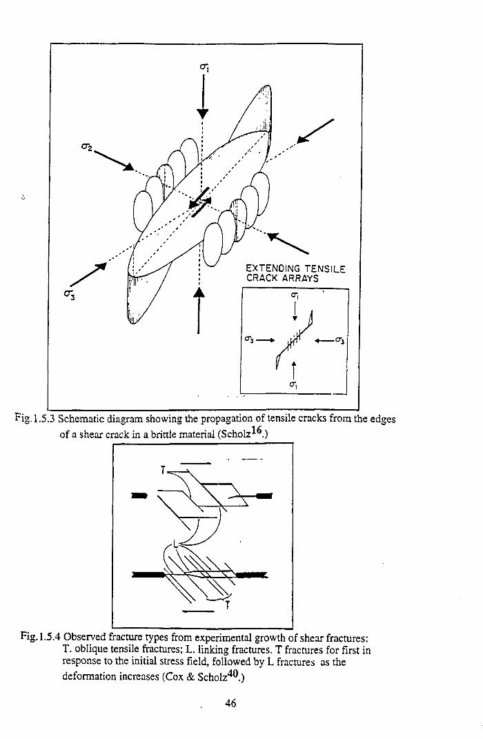
Fig. 1.5.3 Schematic diagram showing the propagation of tensile cracks from the edges of a shear crack in a brittle material (Scholz^.)

Fig. 1.5.4 Observed fracture types from experimental growth of shear fractures: T. oblique tensile fractures; L. linking fractures. T fractures for first in response to the initial stress field, followed by L fractures as thedeformation increases (Cox & Scholz4®.)

46

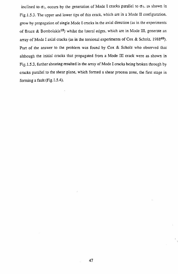
inclined to (Ji, occurs by the generation of Mode I cracks parallel to <3|. as shown in

Fig. 1.5.3. The upper and lower tips of this crack, which are in a Mode II configuration,

grow by propagation of single Mode I cracks in the axial direction (as in the experiments

of Brace & Bombolakis18) whilst the lateral edges, which are in Mode III. generate an

array of Mode I axial cracks (as in the torsional experiments of Cox & Scholz, 198840).

Part of the answer to the problem was found by Cox & Scholz who observed that

although the initial cracks that propagated from a Mode III crack were as shown in

Fig. 1.5.3, further shearing resulted in the array of Mode I cracks being broken through by

cracks parallel to the shear plane, which formed a shear process zone, the first stage in

forming a fault (Fig. 1.5.4).

47

2. TH E IM PORTANCE OF SHEAR DISCONTINUITIES IN HYDROCARBON

RESERVOIRS: A CRITIQUE

2.1 INTRODUCTION

In the province of hydrocarbon reservoir fields, shear discontinuities can exert major

influences on scales ranging from far-field, major tectonic basin-bounding faults, down to

near-wellbore structures associated with failure zones resulting from imbalances between

the uncontrollable factors of earth stresses, rock strength and pore pressure, and the

controllable factors of wellbore fluid pressure, and mud chemical composition. In

addition, shear discontinuities can be beneficial, for example in their role as important

structural oil and gas traps, or indeed disadvantageous, for example when acting to

compartmentalise reservoir horizons, resulting in an increase in the complexity of

required production technology.

In petroleum engineering terms, distinction is made between predominantly matrix

permeability reservoirs and naturally fractured reservoirs, the latter being regarded as

particularly attractive potential economic targets in exploratory ventures. With regard to

naturally fractured reservoirs, reservoir engineers usually make two assumptions

(Aguilera, 198041):

(i) the fractures have a negligible storage capacity and are only channels of high

permeability that allow fluids to flow

(ii) the matrix has an important storage capacity, but a very small permeability

Both assumptions can, however, be misleading when applied to the production

development of naturally fractured reservoirs. With regard to the first presumption, many

reservoirs that produce at high initial rates decline drastically after a short period of time,

due to the producible oil being stored in the fracture system, so that consequently it is

important to estimate oil-in-place reasonably within the fracture network. With regard to

the second assumption, if the permeability of the matrix is very low, then the oil bleed-off

from the matrix into the fractures will be very slow and only the oil originally within the

48

fractures will be produced over a reasonable timescale, so that if the matrix has a

reasonable permeability, then the storage capacity of the matrix becomes of paramount

importance. Thus the storage capacity of naturally fractured reservoirs can vary

extensively, depending on the degree of fracturing in the formation and the value of the

porosity, the greater the value of primary porosity the greater the success of naturally

fractured reservoirs.

This philosophy outlined above serves to highlight the industry's general understanding of

fractured reservoirs, envisaging them as intact rockmass transected by a network of open,

dilatant fracture conduits analogous perhaps to jointing in a granite. To supplement the

"traditional" industry visualisation of fractured reservoirs as regularly jointed rockmasses,

in this second chapter a critique of the role of shear fractures in hydrocarbon reservoirs is

given, concentrating on their control over in situ fluid flow, and on overall deformability

resulting from production-related transients in effective stress. In chapter 4 of this thesis

work experimental investigations into the frictional strength of shear discontinuities

deformed under constant normal displacement boundary conditions more appropriate to

sliding occurring within reservoirs is addressed, whilst in Chapter 6 the sealing potential

of experimentally induced shear fractures similar to naturally occurring granulation seams

is quantified under triaxial stress conditions.

2.2 FAULT SIZE POPULATIONS

Amongst the outstanding problems of reservoir characterisation is that of the quantitative

incorporation of sub-seismic heterogeneities (heterogeneities below the limits of

exploration seismic resolution) into reservoir simulation model gridblocks. In particular,

sub-seismic faults represent one type of heterogeneity for which reliable assessment

methods are a particular prerequisite. The principal questions to be addressed in assessing

the likely effects of sub-seismic faults on reservoir formation permeability (Heath et al,

199442) concern:

(i) the size population of sub-seismic faults

(ii) the hydraulic nature of the faults

49

(iii) the likely effects of a particular fault population of specified hydraulic character on a

particular reservoir sequence

(iv) how the effects of the faults can be expressed in terms of the effective permeabilities

of simulator gridblocks

Whilst prediction of sub-seismic sealing faults has shown considerable advance in recent

years (Childs etal, 199043, Heffer & Bevan, 199044, Yielding etal, 199245, Walsh etal

199446) much greater uncertainty is attached to the actual spatial distributions of such

fault populations. The fluid flow potential of faults, according to Heath et a l42, can be

considered as being either hydraulically active or passive. Hydraulically active faults are

defined as, "those in which the fault surfaces or fault zones have a permeability, or

transmissibility, different from those of the host rocks," so that such faults may be either

sealing, or may channnelise fluid flow. The various mechanisms o f fault sealing are

considered in section 2.3 below.

Hydraulically passive fault surfaces are defined as, "those in which the effect of the faults

is limited to the geometric effects of variable fault offsets on the juxtapositions across the

fault surfaces of permeable and impermeable host rock units." As such, these effects are

strongly sequence dependent, and may decrease or indeed increase connectivity (Knott,

199347). Realistic input of fault geometries and properties in simulation studies should be

followed by calculation of the differences between effective permeabilities of unfaulted

matrix volumes and their faulted equivalents. Heath et al 42 report on investigations into

the hydraulic effects of populations of impermeable sub-seismic faults in lithologically

homogeneous sandstone reservoir formations. Thus they do not consider the role of faults

as seals in the sense of hydraulically isolating a volume of fluid, but consider faults only

as sealing surfaces, or impermeable barriers or baffles, which increase the tortuosity of a

flow path within a connected volume of fluid, but are not necessarily capable of

supporting large pressure differences. Instead, they have attempted to incorporate fault

population statistics in an effort to assess their likely hydraulic impact. Prior to a brief

outline of Heath et al 's results, a short description of fault size population systematics

will be given with special regard to results obtained from hydrocarbon reservoirs.

50

Fault size populations have been demonstrated to be fractal or scale invariant systems

(see section 6.5.1) over a range o f scales from mm to km of fault displacement

(references 43 to 46 and Marrett & Allmendinger, 199148). A scale invariant set has the

same relative numbers of large and small elements at all scales between the upper and

lower fractal limits, and is expressed by a power law distribution where the number of

objects "N" of size "s" or greater is given by:

N = a.s *D .......... Eqn.2.2.1

a : a variable dependent on sample size

D : the fractal dimension of the set

Eqn.2.2.1 can be expressed as a straightline curve on a plot of log(N) versus log(s)which

is the customary way to plot fault population data:

log(N) = log(a) -D .log(s) .......... Eqn.2.2.2

where "a” is a function of fault density for a sample of given size. Walsh et al 46 provide

a succinct summary of the various fault population databases utilised in the literature. An

example dataset might be fault throws encountered on a sample line across a map. By

taking account of the sampled line length, the ordinate can be linearly scaled to

cumulative fault density ( usually referred to as "CUMFD") with units of number of faults

per km of sample line length, and when areas or volumes are sampled the ordinate can be

scaled to express fault densities in terms of the fault trace length per square km of

sampled horizon (km/km2) or the fault surface area per cubic km of sampled volume

(km2/km 3). Population curves derived from seismic data have an additional left hand

shallow segment (Fig.2.2.1) at displacements below the limits of seismic resolution

(approximately 20msecs TWTT for many seismic datasets, Heath et al 42, which for

51

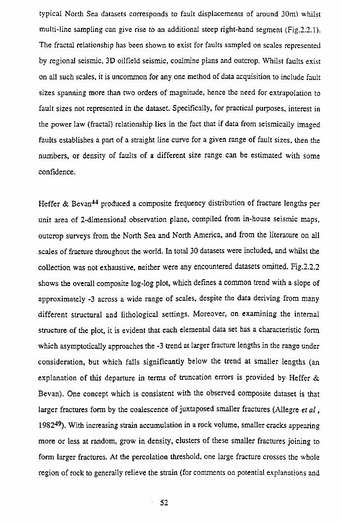
typical North Sea datasets corresponds to fault displacements of around 30m) whilst

multi-line sampling can give rise to an additional steep right-hand segment (Fig.2.2.1).

The fractal relationship has been shown to exist for faults sampled on scales represented

by regional seismic, 3D oilfield seismic, coalmine plans and outcrop. Whilst faults exist

on all such scales, it is uncommon for any one method of data acquisition to include fault

sizes spanning more than two orders of magnitude, hence the need for extrapolation to

fault sizes not represented in the dataset. Specifically, for practical purposes, interest in

the power law (fractal) relationship lies in the fact that if data from seismically imaged

faults establishes a part of a straight line curve for a given range of fault sizes, then the

numbers, or density of faults of a different size range can be estimated with some

confidence.

Heffer & Bevan44 produced a composite frequency distribution of fracture lengths per

unit area of 2-dimensional observation plane, compiled from in-house seismic maps,

outcrop surveys from the North Sea and North America, and from the literature on all

scales of fracture throughout the world. In total 30 datasets were included, and whilst the

collection was not exhaustive, neither were any encountered datasets omitted. Fig.2.2.2

shows the overall composite log-log plot, which defines a common trend with a slope of

approximately -3 across a wide range of scales, despite the data deriving from many

different structural and lithological settings. Moreover, on examining the internal

structure of the plot, it is evident that each elemental data set has a characteristic form

which asymptotically approaches the -3 trend at larger fracture lengths in the range under

consideration, but which falls significantly below the trend at smaller lengths (an

explanation of this departure in terms of truncation errors is provided by Heffer &

Bevan). One concept which is consistent with the observed composite dataset is that

larger fractures form by the coalescence of juxtaposed smaller fractures (Allegre et a l ,

198249). With increasing strain accumulation in a rock volume, smaller cracks appearing

more or less at random, grow in density, clusters of these smaller fractures joining to

form larger fractures. At the percolation threshold, one large fracture crosses the whole

region of rock to generally relieve the strain (for comments on potential explanations and

52

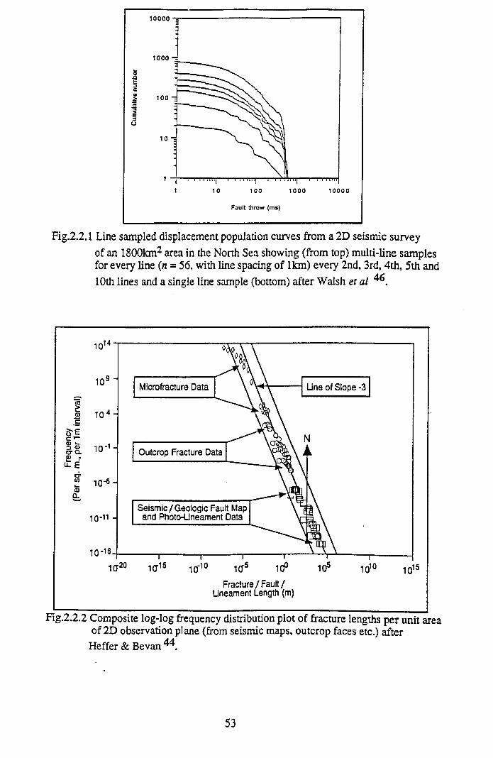
Fig.2.2.1 Line sampled displacement population curves from a 2D seismic surveyof an 1800km2 area in the North Sea showing (from top) multi-line samples for every line (n = 56, with line spacing of 1km) every 2nd, 3rd, 4th, 5th and10th lines and a single line sample (bottom) after Walsh et al 4<\

Fig.2.2.2 Composite log-log frequency distribution plot of fracture lengths per unit area of 2D observation plane (from seismic maps, outcrop faces etc.) after

Heffer & Bevan 44.

53

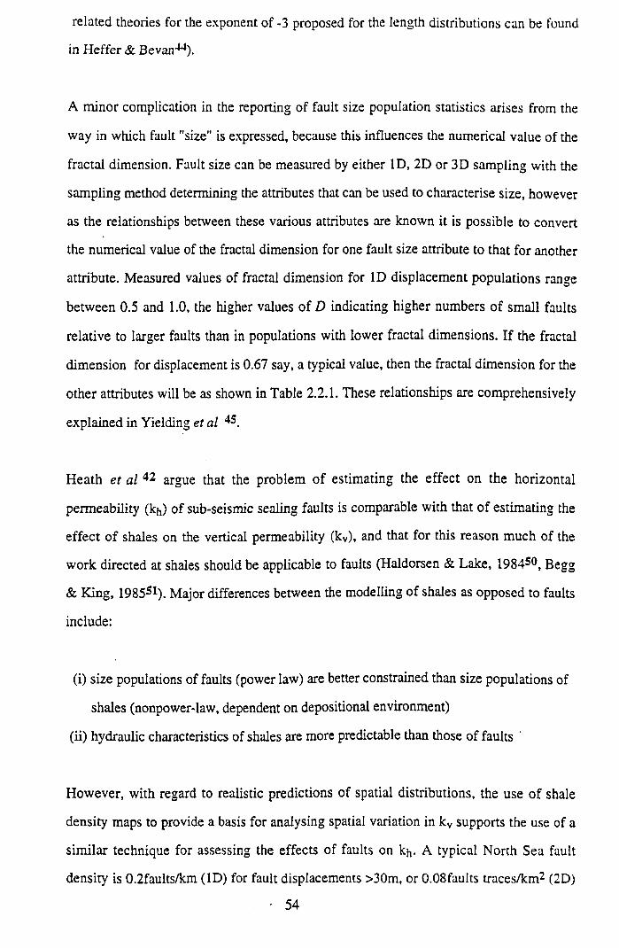
related theories for the exponent of -3 proposed for the length distributions can be found

in Heffer & Bevan44).

A minor complication in the reporting of fault size population statistics arises from the

way in which fault "size" is expressed, because this influences the numerical value of the

fractal dimension. Fault size can be measured by either ID, 2D or 3D sampling with the

sampling method determining the attributes that can be used to characterise size, however

as the relationships between these various attributes are known it is possible to convert

the numerical value of the fractal dimension for one fault size attribute to that for another

attribute. Measured values of fractal dimension for ID displacement populations range

between 0.5 and 1.0, the higher values of D indicating higher numbers of small faults

relative to larger faults than in populations with lower fractal dimensions. If the fractal

dimension for displacement is 0.67 say, a typical value, then the fractal dimension for the

other attributes will be as shown in Table 2.2.1. These relationships are comprehensively

explained in Yielding et al 45.

Heath et al 42 argue that the problem of estimating the effect on the horizontal

permeability (kh) of sub-seismic sealing faults is comparable with that o f estimating the

effect o f shales on the vertical permeability (kv), and that for this reason much of the

work directed at shales should be applicable to faults (Haldorsen & Lake, 198450, Begg

& King, 1985s1). Major differences between the modelling of shales as opposed to faults

include:

(i) size populations of faults (power law) are better constrained than size populations of

shales (nonpower-law, dependent on depositional environment)

(ii) hydraulic characteristics of shales are more predictable than those of faults

However, with regard to realistic predictions of spatial distributions, the use of shale

density maps to provide a basis for analysing spatial variation in kv supports the use of a

similar technique for assessing the effects of faults on kh- A typical North Sea fault

density is 0.2faults/km (ID) for fault displacements >30m, or 0.08faults traces/km2 (2D)

• 54

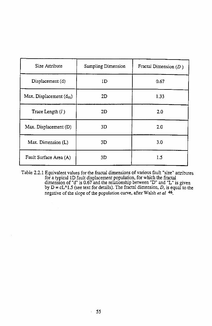
Size Attribute Sampling Dimension Fractal Dimension (D )

Displacement (d) ID 0.67

Max. Displacement (dm) 2D 1.33

Trace Length ( /) 2D 2.0

Max. Displacement (D) 3D 2.0

Max. Dimension (L) 3D 3.0

Fault Surface Area (A) 3D 1.5

Table 2.2.1 Equivalent values for the fractal dimensions of various fault "size" attributes for a typical ID fault displacement population, for which the fractal dimension of "d" is 0.67 and the relationship between "D" and "L" is given by D = cLA1.5 (see text for details). The fractal dimension, D, is equal to the negative of the slope of the population curve, after Walsh et al 46.

55

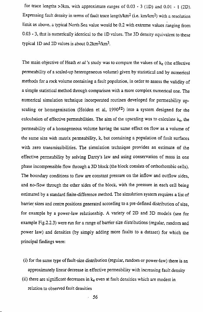
for trace lengths >3km, with approximate ranges of 0.03 - 3 (ID ) and 0 .0 1 - 1 (2D).

Expressing fault density in terms of fault trace length/km(i) 2 (i.e. km/km2) with a resolution

limit as above, a typical North Sea value would be 0.2 with extreme values ranging from

0.03 - 3, that is numerically identical to the ID values. The 3D density equivalent to these

typical ID and 2D values is about 0.2km2/km3.

The main objective of Heath et a l 's study was to compare the values of ke (the effective

permeability of a scaled-up heterogeneous volume) given by statistical and by numerical

methods for a rock volume containing a fault population, in order to assess the validity of

a simple statistical method through comparison with a more complex numerical one. The

numerical simulation technique incorporated routines developed for permeability up-

scaling or homogenisation (Holden et al, 199052) into a system designed for the

calculation of effective permeabilities. The aim of the upscaling was to calculate ke, the

permeability of a homogeneous volume having the same effect on flow as a volume of

the same size with matrix permeability, k, but containing a population of fault surfaces

with zero transmissibilities. The simulation technique provides an estimate of the

effective permeability by solving Darcy's law and using conservation of mass in one

phase incompressible flow through a 3D block (the block consists of orthorhombic cells).

The boundary conditions to flow are constant pressure on the inflow and outflow sides,

and no-flow through the other sides o f the block, with the pressure in each cell being

estimated by a standard finite-difference method. The simulation system requires a list of

barrier sizes and centre positions generated according to a pre-defined distribution of size,

for example by a power-law relationship. A variety of 2D and 3D models (see for

example Fig.2.2.3) were run for a range of barrier size distributions (regular, random and

power law) and densities (by simply adding more faults to a dataset) for which the

principal findings were:

(i) for the same type of fault-size distribution (regular, random or power-law) there is an

approximately linear decrease in effective permeability with increasing fault density

(ii) there are significant decreases in ke even at fault densities which are modest in

relation to observed fault densities

56

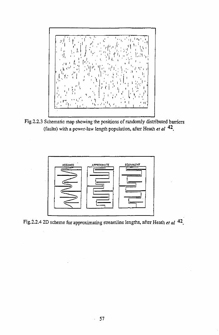
. ( ¡ ' I v Y ï ; ^ ' :

-----n— ' ,—■ ■. I 1 ''u ■, »

1 . • '!

i ' i ’ ' V , : ' i ' ' 1' ! ,

( ' i " '. . ' *1. .(

• :, M . 1

I K ’ I ••i .

V , ,

• ; Y

1 \ •! 1 • ■ i . , i l ' -i ;| ■ i.

i 1 '

‘ | . 1 1. '

. 1 > n •’• . • 1 .1

■ i i 1 ■ ■i , i, i

1 « • • »

Fig.2.2.3 Schematic map showing the positions of randomly distributed barriers (faults) with a power-law length population, after Heath et al

Fig.2.2.4 2D scheme for approximating streamline lengths, after Heath et al ^2

57

The statistical simulation method employed by Heath et a l42 borrowed from recent

developments in the determination of the effects of discontinuous shales on single-phase

vertical permeability (Haldorsen & Lake50, Begg & King51). Since discontinuous barriers

represented by impermeable vertical faults might well be expected to have a similar effect

on kh as do shales on kv, statistical simulation techniques might provide a simple

alternative to the numerical simulation of fault systems. Heath et al 42 estimated the

impact of faults on kh using a slightly modified version of the "statistical streamline"

technique developed by Begg & King51, which is itself a development of the method

described by Haldorsen & Lake50. The modification is introduced to take account of the

power-law size distributions of faults, for reasons fully explained in Heath et al 42. The

statistical streamline technique is based on the premise that the presence of barriers

increases the tortuosity of flow paths within a rock volume. Tortuosity estimates (that is

the increase in the length of streamlines due to the presence of permeability barriers) can

be simply made using an approximation of average streamline length through, or across, a

volume or area of interest (Fig.2.2.4). The approximation is valid for barriers with a

regular size distribution and requires only a knowledge of the density of the barriers and

of the mean barrier length, L, and width, W, (the assumption is made that the faults are

square plates with L=W). However, incorporation of mean lengths and densities can lead

to significant errors when applied to barriers with many small faults relative to large ones

( that is negative exponential and power law expressions) resulting in the impact of large

barriers being underestimated. In such cases a better approximation of the extension to

the streamline length is obtained by calculating on a fault by fault basis, with such

explicit incorporation of fault sizes being found to increase the tortuosity significantly

more than the use of mean fault sizes. The consequence of using mean as opposed to

explicit fault sizes is evident in the observed reduction of ke/k ratios by * 100% at higher

fault densities (ke refers to the faulted volume effective permeability, k refers to the

unfaulted volume matrix permeability).

58

Results from both the numerical and the statistical simulations were found to be closely

comparable for power-law size distributions of barriers (faults) in both 2D and 3D, from

which Heath et al concluded that acceptable results can be obtained for fault populations

by using the simple statistical method. Having established the validity of the modified

statistical streamline technique for assessing the effect of populations of sealing faults on

ke, the method was used to quantify these effects for realistic ranges of fault densities and

population slopes, for both 3D (Fig.2.2.5a) and 2D (Fig.2.2.5b) cases. The results indicate

th a t:

(i) for realistic values of fault densities, populations of sub-seismic sealing faults have a

significant impact on effective permeabilities, with ke/k values ranging down to

*0.001 for the 2D model at high densities.

(ii) for the same population exponents and fault densities, ke values for 2D models are

lower than those for 3D models, consistent with conclusions drawn from statistical

simulation of shale sequences

(iii) ke appears more sensitive to variation in fault densities than to variation in the power

law exponent, due mainly, according to Heath et al, to the greater impact on flow of

larger faults than to the more numerous smaller ones, so that ke shows a wide range

because of the wide range in likely fault densities.

2.3 FAULT SEALING POTENTIAL

Faulting forms one of the foremost controls on the distribution, size and internal structure

of hydrocarbon reservoirs. Whilst the role of fault zones in providing both a pathway for

secondary hydrocarbon migration and a seal to hydrocarbon accumulations has long been

recognised, very little attention has been focused on the processes contributing to the

production of fault rocks, and their possible influences on sealing properties. Whilst

section 2.2 above concentrated on the influence of fault size populations on reservoir

formation permeability, in this section the finite hydraulic nature of the fault zones

themselves will be considered.

59

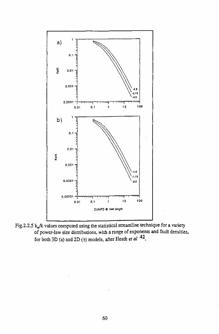
Fig.2.2.5 kg/k values computed using the statistical streamline technique for a variety of power-law size distributions, with a range of exponents and fault densities, for both 3D (a) and 2D (b) models, after Heath et al

60

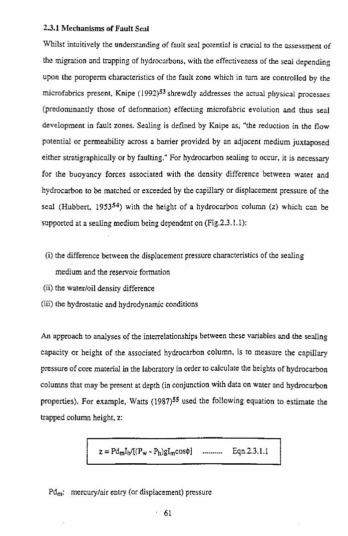
2.3.1 M echanisms of Fault Seal

Whilst intuitively the understanding of fault seal potential is crucial to the assessment of

the migration and trapping of hydrocarbons, with the effectiveness of the seal depending

upon the poroperm characteristics of the fault zone which in turn are controlled by the

microfabrics present, Knipe (1992)53 shrewdly addresses the actual physical processes

(predominantly those of deformation) effecting microfabric evolution and thus seal

development in fault zones. Sealing is defined by Knipe as, "the reduction in the flow

potential or permeability across a barrier provided by an adjacent medium juxtaposed

either stratigraphically or by faulting." For hydrocarbon sealing to occur, it is necessary

for the buoyancy forces associated with the density difference between water and

hydrocarbon to be matched or exceeded by the capillary or displacement pressure of the

seal (Hubbert, 195354) with the height of a hydrocarbon column (z) which can be

supported at a sealing medium being dependent on (Fig.2.3.1.1):

(i) the difference between the displacement pressure characteristics of the sealing

medium and the reservoir formation

(ii) the water/oil density difference

(iii) the hydrostatic and hydrodynamic conditions

An approach to analyses of the interrelationships between these variables and the sealing

capacity or height of the associated hydrocarbon column, is to measure the capillary

pressure of core material in the laboratory in order to calculate the heights of hydrocarbon

columns that may be present at depth (in conjunction with data on water and hydrocarbon

properties). For example, Watts (1987)55 used the following equation to estimate the

trapped column height, z:

z = PdmIh/[(Pw - Pb)gImCos<M .......... Eqn.2.3.1.1

Pdm: mercury/air entry (or displacement) pressure

61

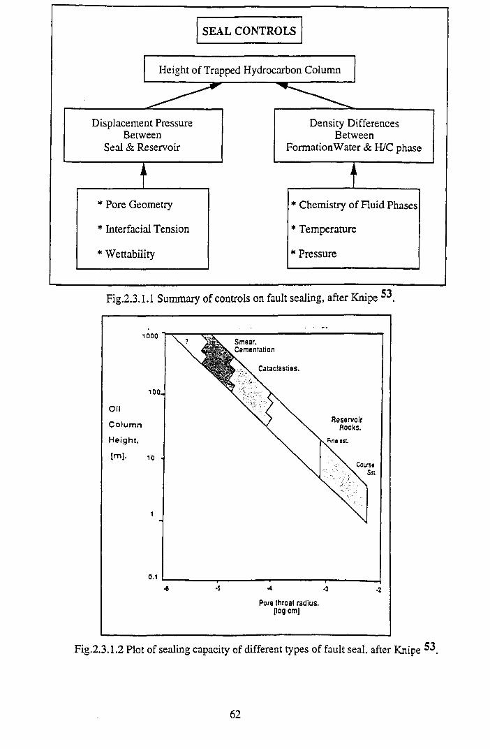
SEAL CONTROLS

Fig.2.3.1.1 Summary of controls on fault sealing, after Knipe ^3.

Fig.2.3.1.2 Plot of sealing capacity of different types of fault seal, after Knipe ^3

62

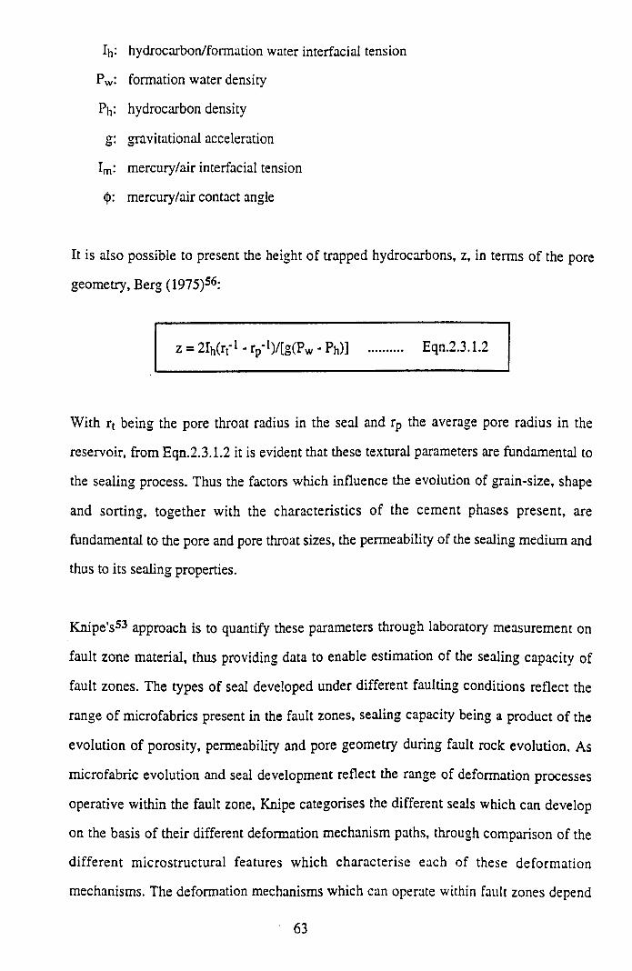
Ih: hydrocarbon/formation water interfacial tension

Pw: formation water density

Ph: hydrocarbon density

g: gravitational acceleration

Im: mercury/air interfacial tension

0: mercury/air contact angle

It is also possible to present the height of trapped hydrocarbons, z, in terms of the pore

geometry, Berg (1975)56:

z = 2Ih(rt*1 - rp-l)/[g(Pw - Ph)j .......... Eqn.2.3.1.2

W ith rt being the pore throat radius in the seal and rp the average pore radius in the

reservoir, from Eqn.2.3.1.2 it is evident that these textural parameters are fundamental to

the sealing process. Thus the factors which influence the evolution of grain-size, shape

and sorting, together with the characteristics of the cement phases present, are

fundamental to the pore and pore throat sizes, the permeability of the sealing medium and

thus to its sealing properties.

Knipe's53 approach is to quantify these parameters through laboratory measurement on

fault zone material, thus providing data to enable estimation of the sealing capacity of

fault zones. The types of seal developed under different faulting conditions reflect the

range of microfabrics present in the fault zones, sealing capacity being a product o f the

evolution of porosity, permeability and pore geometry during fault rock evolution. As

microfabric evolution and seal development reflect the range of deformation processes

operative within the fault zone, Knipe categorises the different seals which can develop

on the basis of their different deformation mechanism paths, through comparison of the

different microstructural features which characterise each of these deformation

mechanisms. The deformation mechanisms which can operate within fault zones depend

63

on the interaction of the material properties (mineralogy, texture, porosity, permeability)

and the environmental conditions (effective stress, temperature). Rock deformation

mechanisms can be divided into three categories, based on the recognition of

distinguishing microstructural features: frictional sliding, fracture processes and

cataclastic flow; diffusive mass transfer (pressure solution); crystal plastic processes,

which are reviewed in greater detail in section 1.2. As the microstructural changes

associated with each mechanism are different, the type o f sealing arising from the

operation of each also differs, so that establishing the deformation mechanisms operating

in different faults is therefore critical to the assessment of seal development. Based on the

above methodology, Knipe groups fault seals into three broad categories:

(i) Porosity collapse seals. Changes in the permeability, porosity and sealing potential

within the fault zone are induced by changes in the pore volume, shape and size by

grain refinement and rearrangement associated with frictional sliding and/or the

cataclasis, dissolution, alteration and plastic deformation of grains/fragments within

the fault zone. Shale smear seals would fall in this category.

(ii) Cement seals. Changes in the permeability, porosity and sealing potential arising

from the growth of new phases within and adjacent to fault zones. Asphalt/tar

impregnations are included as cement seals here.

(iii) Juxtaposition seals. Seals produced by the juxtaposition of two lithologies with

different capillary pressures. In this case seal characteristics are largely independent

of the faulting processes and the fault only serves to juxtapose the two lithologies

with either different pore geometries and/or fluid pressures.

Whilst the sealing properties of a single fault may in part be due to all these factors if the

range o f conditions and lithologies involved are large, different types of fault rock and

hence different characteristic seals are likely to develop in different situations, so that

information from the fault rock microstructure analyses (grain size, shape, sorting, pore

geometry etc.) can be used to estimate the sealing capacity of the zone. The sealing

capacities of the three categories listed above, or the equivalent hydrocarbon column

64

heights which these seals could support, were calculated by Knipe, using Eqn.2.3.1.2.

Values for the pore size and pore throat diameters were based on those measured from

mercury injection tests, and from SEM and TEM micrographs, whilst the values of the

other important variables influencing the sealing capacity (formation water and

hydrocarbon densities, the hydrocarbon interfacial tension) enclosed the range commonly

encountered in reservoirs. The results of these estimates of sealing capacity are shown

schematically in Fig.2.3.1.2, and indicate that the most effective seals are those with the

smallest pore throats. The distribution of seals along faults is known as a fundamental

control on their trapping potential. With this in mind, Knipe also discusses briefly the

factors most likely to cause the seal type to vary, not only between different faults, but

also along individual faults, including:

(i) the distribution of lithologies intersecting the fault planes

(ii) the propagation and displacement mechanisms of the faults (their deformation

mechanism histories)

(iii) the nature of the fluid flow along the fault

(iv) the fault plane geometry

W hilst the above analysis of faulting processes provides a useful framework for

categorising fault seal on the basis of deformation mechanisms, in the literature relating

to hydrocarbon reservoir degradation, three principal fault seal types are recognised: (i)

diagenetic/cement seals; (ii) clay smear seals; (iii) cataclastic seals. A brief review of

each type will be given below, concentrating on (iii), as cataclastic shear bands generated

experimentally as part of this thesis work are described in chapter six (see section 6.4).

2.3.2 Fault-related Diagenesis

Fault zones are often cited as simple barriers/seals or conversely as permeable migration

pathways/conduits for sub-surface fluids such as brines and hydrocarbons, with cataclasis

and diffusive mass transfer being the most important deformation mechanisms which

induce complex textural changes in the vicinity of fault zones. Whilst the dilational

nature of cataclastic fracturing increases the porosity and permeability of the fault zones

65

to promote fluid flow, however intense fracturing and grain-size reduction reduce the size

of inter-granular pore space, leading to permeability reduction. Low rates of cementation

and pressure solution may produce low strength contacts between clasts in a gouge, so

that, under such conditions, some strain may be accommodated by sliding along the edges

of the clasts, enabling inter-granular pore-spaces to open and close during macroscopic

fault displacement (Knipe53). The influx of fluid into dilational pore spaces aids the mass

transport of material in solution which may lead to the precipitation of porosity occluding

cements within the fault zone. The material involved in the mass transfer process may be

provided by the action of pressure solution which also leads to a reduction in porosity and

permeability due to chemical-induced grain compaction.

The precipitation of cements along and adjacent to a fault zone, resulting in changes in

porosity and permeability controlling the sealing capacity, can be induced by changes in

the fluid pressure and temperature experienced by fluids during the faulting process.

Sibson (1981)57 first presented a detailed analysis of the fluid pressure cycles associated

with faulting. Models were presented (Sibson, 19903**) for the behaviour of faults as

"valves" which control the channelling of fluids in fault zones and as "pumps" which

cause expulsion of accumulated fluids. Direct evidence that channel flow of aqueous

fluids accompanies shallow crustal faulting comes from the observation of transitory

surface effusions following some moderate to large earthquakes in consolidated rocks,

and the textural characteristics o f the hydrothermal vein systems often found associated

with ancient exhumed faults. Such phenomena were considered in relation to two

alternative models. In the first, the transitory post-seismic flow can be readily interpreted

in terms of the "dilatancy/fluid diffusion" hypothesis with fluid expulsion resulting from

the collapse of a broad network of pre-failure dilatant fractures enclosing rigid crustal

blocks, in response to the decrease in deviatoric stress accompanying slip. Essentially the

fault/fracture system is acting as a "pump" with aqueous fluids being slowly drawn into

the dilatant fracture system as elastic strain accumulates, to be rapidly expelled in a pulse

every time slip occurs on the main fault as shown schematically in Fig.2.3.2.1(a). In the

second, diametrically opposed model, the fault/fracture system functions as a self-sealing

"valve" on a fluid reservoir, as shown in Fig.2.3.2.1(b). In such a model, it is the slow

66

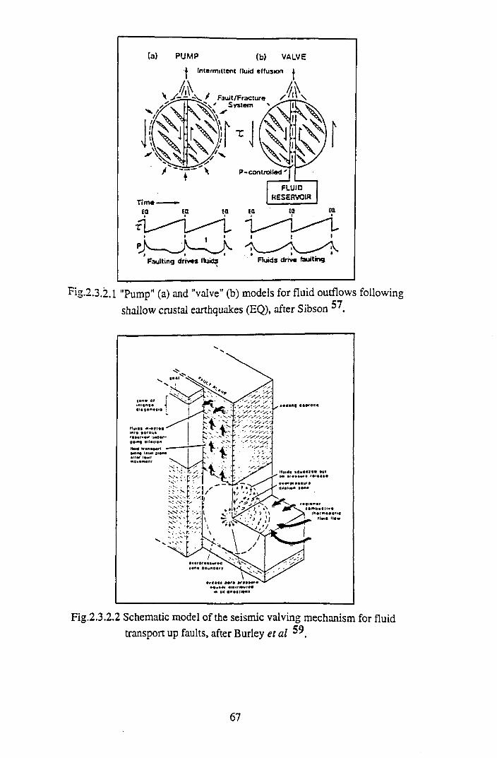
Fig.2.3.2.1 "Pump" (a) and "valve" (b) models for fluid outflows following shallow crustal earthquakes (EQ), after Sibson

Fig.2.3.2.2 Schematic model of the seismic valving mechanism for fluid transport up faults, after Burley et al

67

build-up of fluid pressure that periodically induces fault slip, rather than the other way

around. Once failure has occurred (in accordance with the effective stress law,

t=T 0+n(CTn-p)) freshly created fracture permeability on the fault and allied fractures

allows fluids to escape, so that pressure in the reservoir drops, progressive deposition of

hydrothermal minerals re-seals the fracture system, and the whole cycle may be repeated.

Seismic valving was propounded by Burley et al (1989)59 as an elegant mechanism for

explaining the timing of diagenesis in the Tartan field and adjacent Witch Ground Graben

(UK North Sea) as constrained from combined cathodoluminescence microscopy and

fluid inclusion studies of successive cement generations. The sequence o f mineral

cements was found to be cyclical, such cyclicity suggesting multiple injection of similar

pore fluids, explainable through repeated movement of similar pore fluids along fault

conduits. A mechanism involving inflation of pores and microfracturing in mudrocks

juxtaposed against the sealing faults that delineate the Tartan structure is envisaged as the

main process involved in the emplacement of fluids in the Tartan reservoir (Fig.2.3.2.2).

Dilation and microfracturing result simply from overpressure induced by a compactional

thermobaric drive. As the fluid pressure in the mudrocks juxtaposed against the sealing

faults gradually rises, frictional resistance on the fault plane decreases until the point is

reached where the rising shear stress exceeds the frictional resistance. The ensuing rapid

release of shear stress as failure occurs relaxes the inflated pores and microfractures

within the dilatant zone. Pore fluids are rapidly expelled along the direction o f least

resistance, fluid transport from the collapsing dilatant zone thus taking place along the

main fault plane and adjacent parallel fractures. After fluid escape, pressure in the dilatant

zone drops, the fault re-seals and the thermobaric drive restarts the process. Thus in this

model, it is the gradual build-up of overpressure that periodically induces fault failure.

Sibson also emphasised the role of dilation sites created along the fault zones during the

displacement events (e.g. dilational jogs, see Sibson, 198560) as locations where rapid

fluid influx and pressure drops can induce preferential precipitation. Knipe53 notes that

the dilation magnitude together with the fluid pressure and permeability changes during

faulting events, will all influence the volume of cement produced, for example in fault

68

zones where both dilation and fluid pressure changes are large, very rapid precipitation

can result with the production of a breccia composed of rock fragments floating in cement

(termed implosion breccias by Sibson, 198661). Implosion breccias are related to the

collapse of the wall rock into dilation sites generated by the slip events. In contrast, for

slip events in which fault zone dilation at the time of precipitation is suppressed, so that

cataclastic fragments remain in contact to provide a load-bearing framework, cement

precipitation will create overgrowths within the pores of the cataclasite. Irrespective of

the detailed mechanism of cement generation involved, KnipeS3 considers the reduction

in both porosity and permeability through cementation to be large, with for example 20%

initial porosity sandstones typically showing reductions to <1%, with attendant

permeability diminishment of over an order of magnitude.

2.3.3 Shale Smears

"Shale smear" is a general term used to describe a shale or clay layer intervening between

sandstone units juxtaposed across a fault, in the manner of fault-plane "fillings" rather

than fault gouges (Smith, 198062). Whilst early descriptions of shale smears (for example

Weber et a l , 197863) are of occurrences on growth faults, the examples described by

Lindsay et a l , 199164 are the result of tectonic faulting of lithified sediments. They

examined the nature and systematics of shale smears in working quarries exposing

Westphalian sandstone/shale sequences offset by faults of up to 15m throw. The smears

occurred on sandstone/sandstone fault surfaces, some extending from footwall to

hangingwall cut-offs of the shale source layer. The smears hydraulically separate

sandstone units in footwall and hangingwall which, in the absence of shale smearing,

would be expected to be hydraulically connected across the fault. Three distinct types of

shale smear were recognised, and named according to the proposed mechanism of their

formation: (i) abrasion smear; (ii) shear zone smear; (iii) injection smear.

Abrasion smears were found to be the most common and occurred as uniform, wafer-thin

(<lm m ) films or veneers on sandstone fracture surfaces. Surface markings such as striae

and tool marks from embedded breccia clasts were commonly observed. Relative

movement of shale past a sandstone surface leaves a thin veneer of shale on the sandstone

69

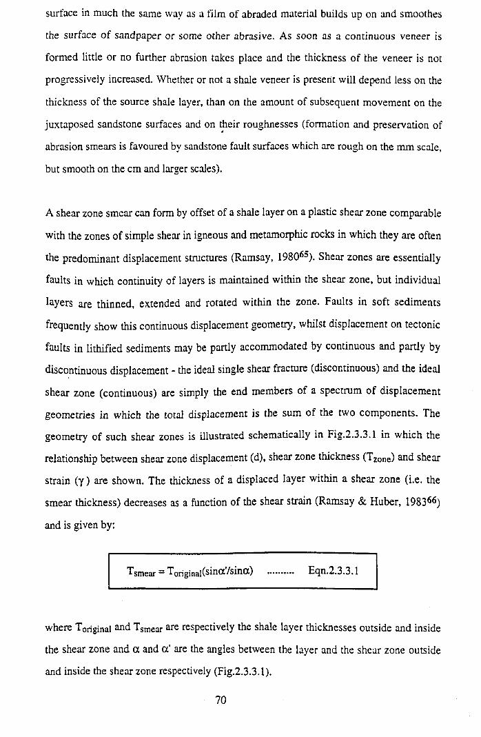
surface in much the same wav as a film of abraded material builds up on and smoothes

the surface o f sandpaper or some other abrasive. As soon as a continuous veneer is

formed little or no further abrasion takes place and the thickness of the veneer is not

progressively increased. Whether or not a shale veneer is present will depend less on the

thickness of the source shale layer, than on the amount of subsequent movement on the

juxtaposed sandstone surfaces and on their roughnesses (formation and preservation of

abrasion smears is favoured by sandstone fault surfaces which are rough on the mm scale,

but smooth on the cm and larger scales).

A shear zone smear can form by offset of a shale layer on a plastic shear zone comparable

with the zones of simple shear in igneous and metamorphic rocks in which they are often

the predominant displacement structures (Ramsay, 198065). Shear zones are essentially

faults in which continuity of layers is maintained within the shear zone, but individual

layers are thinned, extended and rotated within the zone. Faults in soft sediments

frequently show this continuous displacement geometry, whilst displacement on tectonic

faults in lithified sediments may be partly accommodated by continuous and partly by

discontinuous displacement - the ideal single shear fracture (discontinuous) and the ideal

shear zone (continuous) are simply the end members of a spectrum of displacement

geometries in which the total displacement is the sum of the two components. The

geometry of such shear zones is illustrated schematically in Fig.2.3.3.1 in which the

relationship between shear zone displacement (d), shear zone thickness (Tzone) and shear

strain (y ) are shown. The thickness of a displaced layer within a shear zone (i.e. the

smear thickness) decreases as a function of the shear strain (Ramsay & Huber, 198366)

and is given by:

"f smear = ^originalisi^tx/sinOt) .......... Eqn.2.3.3.1

where Toriginal and Tstnear are respectively the shale layer thicknesses outside and inside

the shear zone and a and a ' are the angles between the layer and the shear zone outside

and inside the shear zone respectively (Fig.2.3.3.1).

70

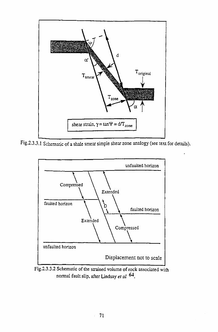
Fig.2.3.3.1 Schematic of a shale smear simple shear zone analogy (see text for details).

unfaulted horizon

Displacement not to scale

Fig.2.3.3.2 Schematic of the strained volume of rock associated with normal fault slip, after Lindsay et al 64.

71

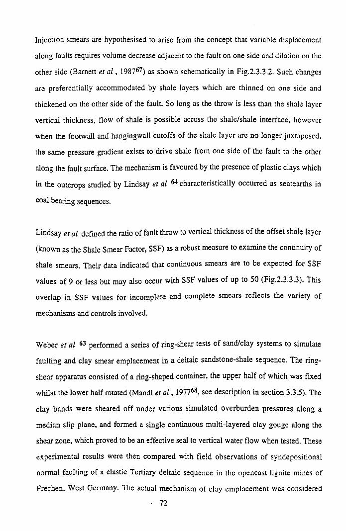
Injection smears are hypothesised to arise from the concept that variable displacement

along faults requires volume decrease adjacent to the fault on one side and dilation on the

other side (Barnett et a l , 198767) as shown schematically in Fig.2.3.3.2. Such changes

are preferentially accommodated by shale layers which are thinned on one side and

thickened on the other side of the fault. So long as the throw is less than the shale layer

vertical thickness, flow of shale is possible across the shale/shale interface, however

when the footwall and hangingwall cutoffs of the shale layer are no longer juxtaposed,

the same pressure gradient exists to drive shale from one side of the fault to the other

along the fault surface. The mechanism is favoured by the presence of plastic clays which

in the outcrops studied by Lindsay et al 64 characteristically occurred as seatearths in

coal bearing sequences.

Lindsay et al defined the ratio of fault throw to vertical thickness of the offset shale layer

(known as the Shale Smear Factor, SSF) as a robust measure to examine the continuity of

shale smears. Their data indicated that continuous smears are to be expected for SSF

values of 9 or less but may also occur with SSF values of up to 50 (Fig.2.3.3.3). This

overlap in SSF values for incomplete and complete smears reflects the variety of

mechanisms and controls involved.

Weber et al 63 performed a series of ring-shear tests of sand/clay systems to simulate

faulting and clay smear emplacement in a deltaic sandstone-shale sequence. The ring-

shear apparatus consisted of a ring-shaped container, the upper half of which was fixed

whilst the lower half rotated (Mandl et a l , 197768, see description in section 3.3.5). The

clay bands were sheared off under various simulated overburden pressures along a

median slip plane, and formed a single continuous multi-layered clay gouge along the

shear zone, which proved to be an effective seal to vertical water flow when tested. These

experimental results were then compared with field observations of syndepositional

normal faulting of a clastic Tertiary deltaic sequence in the opencast lignite mines of

Frechen, West Germany. The actual mechanism of clay emplacement was considered

72

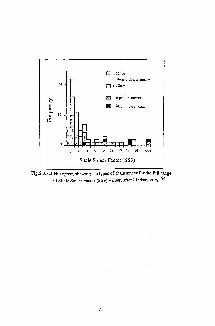
Fig.2.3.3.3 Histogram showing the types of shale smear for the full of Shale Smear Factor (SSF) values, after Lindsay et al

range64

73

probably to be more effective than in the laboratory model, involving a larger amount of

material being squeezed into the fault zone. Clay gouges within the field shear zones

decreased in thickness away from the source beds, and individual clay gouges from

separate source beds coalesced to form one multilayered clay gouge. Thicker shale source

beds provided longer more continuous clay gouges than thinner ones.

2.3.4 Granulation Seams

Volumetrically, planar tectonic features contribute very little to the total porosity of an

aquifer or hydrocarbon reservoir (see discussion in section 2 . 1) with the matrix porosity

being orders of magnitude more important, however matrix porosity between tectonic

surfaces is only effective porosity when these surfaces do not have reduced permeability

characteristics. Whilst the fluid flow characteristics of small-scale sedimentary features

and architecture have received considerable attention, especially with the development of

probe permeametry, the fluid flow characteristics of tectonic surfaces acting as baffles as

opposed to conduits has been largely ignored. Thus whilst the sealing characteristics of

tectonic surfaces have a crucial influence on the overall large scale flow characteristics of

porous media, surprisingly little work has focused on the micromechanics o f the sealing

mechanism. Chapter 7 of this thesis work attempts to address this interesting topic,

through direct quantification of the effective sealing potential of experimentally produced

shear fractures induced under various triaxial stress states, and the relationships between

permeability modification and the nature of the shear debris (artificial fault gouge)

generated.

Fluid flow retardation is associated with various tectonic features (for example pressure

solution seams) however granulation seams are a particularly im portant type of

permeability barrier. They occur as conjugate sets within high porosity sandstones which

form some of the most productive hydrocarbon reservoirs in the North Sea. Though their

displacement is small and width limited on individual seams (both generally < 10mm)

they act as extremely effective permeability barriers and are thus one o f the most

significant types of planar heterogeneity in many massive sandstone hydrocarbon

reservoirs, with otherwise excellent fluid sweep potential. In many of these fields,

74

intersecting granulation seams in three dimensions serve to compartmentalise the

reservoir, such that blocks can often have quite different physico-chemical features (for

example diagenetic histories through differential flow rates of formation fluids'),

poroperm characteristics and can even lack hydrocarbons.

Cataclasis leads to zones of grain rearrangement and comminution which have been

referred to by a plethora of terms as summarised in Table 2.3.4.1. As the terms listed in

this table were applied to specific cases, rather than being intended for general usage,

they tend to be mutually conflicting, and fail to concur with all recorded observations. In

light o f this rather confusing current terminology, partly genetic, partly descriptive, the

term "granulation seam" will be adopted here for such structures, as although perhaps no

more apt than the others, it seems to have achieved more widespread usage in the current

literature. The nature of faulting in porous sandstones is typically as that described for

faults in the Navajo and Entrada sandstones of SE Utah (see Aydin 197870, Aydin &

Johnson, 197876 and Aydin & Reches, 198277). Both sandstones are friable, composed

primarily of quartz and feldspar, and possess porosities of around 25%. Three forms of

faults are recognised in these sandstones (Fig.2.3.4.1): (i) deformation bands; (ii) zones of

deformation bands; (iii) slip surfaces. Each form occurs in dip-slip, strike-slip and

oblique-slip orientations. Small faults occur as deformation bands, about lmm-thick, in

which pores collapse and sand grains fracture and along which there are shear

displacements of the order of a few mm's to cm's (a).'Two or more adjacent deformation

bands (b) that share the same strike and dip form a zone of deformation bands (c). A zone

becomes thicker by the addition of new bands side-by-side. Slip surfaces, pervasive

surfaces of discontinuity in displacement, form at either edge of zones of highly

concentrated deformation bands, and can accommodate large displacements in then order

of several or tens of metres (d). Such subdivisions (Fig.2.3.4.2) were also found

applicable in the high porosity aeolian sandstones (Lower Permian Penrith Sandstone

Formation) at outcrop in NW England and SW Scotland, by Fowles & Burley (1994)78.

With regard to their mechanism of formation, it is well documented in the references

listed in Table2.3.4.1 that cataclasis is the primary deformation mechanism, involving

75

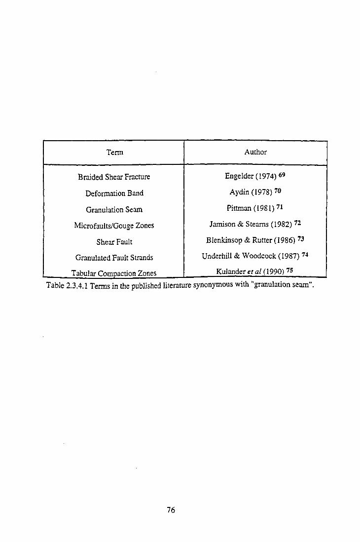
Term Author

Braided Shear Fracture Engelder(1974) 69

Deformation Band Aydin (1978) 70

Granulation Seam Pittman (1981)71

Microfaults/Gouge Zones Jamison & Steams (1982) 72

Shear Fault Blenkinsop & Rutter (1986) 73

Granulated Fault Strands Underhill & Woodcock (1987) 74

Tabular Compaction Zones Kulander etal (1990) 73

Table 2.3.4.1 Terms in the published literature synonymous with "granulation seam".

76

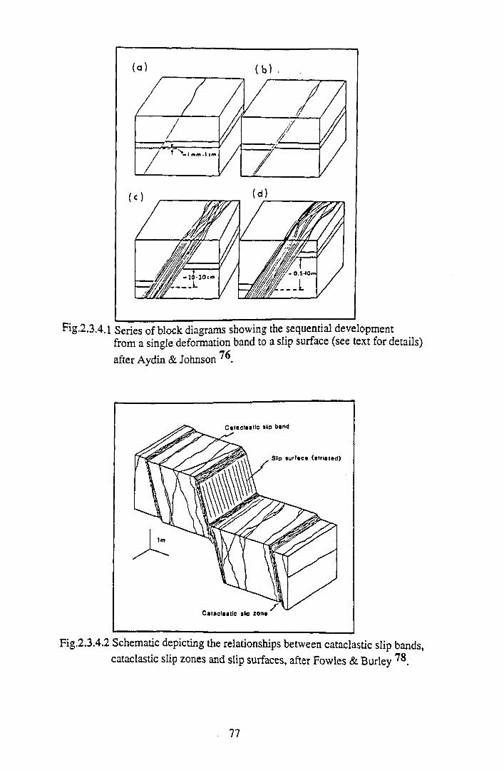
Fig.2.3.4.1 Series of block diagrams showing the sequential developmentfrom a single deformation band to a slip surface (see text for details)

after Aydin & Johnson

Fig.2.3.4.2 Schematic depicting the relationships between cataclastic slip bands, cataclastic slip zones and slip surfaces, after Fowles & Burley ^8

77

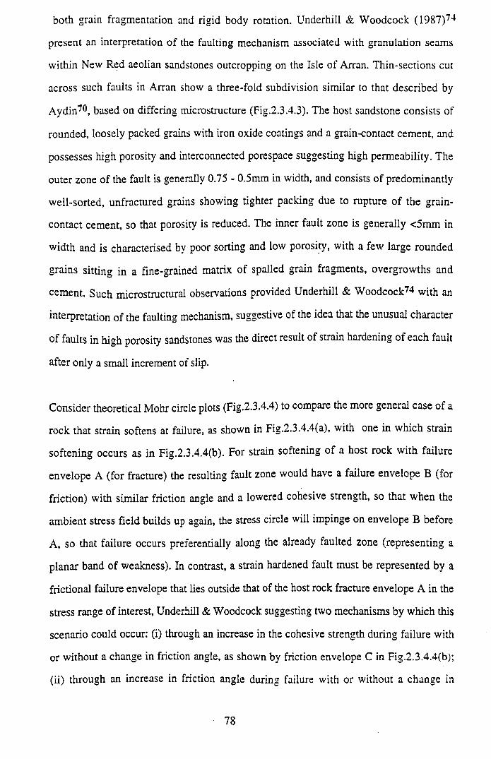
both grain fragmentation and rigid body rotation. Underhill & Woodcock (1987)74

present an interpretation of the faulting mechanism associated with granulation seams

within New Red aeolian sandstones outcropping on the Isle of Arran. Thin-sections cut

across such faults in Arran show a three-fold subdivision similar to that described by

Aydin70, based on differing microstructure (Fig.2.3.4.3). The host sandstone consists of

rounded, loosely packed grains with iron oxide coatings and a grain-contact cement, and

possesses high porosity and interconnected porespace suggesting high permeability. The

outer zone of the fault is generally 0.75 - 0.5mm in width, and consists of predominantly

well-sorted, unfractured grains showing tighter packing due to rupture o f the grain-

contact cement, so that porosity is reduced. The inner fault zone is generally <5mm in

width and is characterised by poor sorting and low porosity, with a few large rounded

grains sitting in a fine-grained matrix of spalled grain fragments, overgrowths and

cement. Such microstructural observations provided Underhill & Woodcock74 with an

interpretation of the faulting mechanism, suggestive of the idea that the unusual character

of faults in high porosity sandstones was the direct result of strain hardening of each fault

after only a small increment of slip.

Consider theoretical Mohr circle plots (Fig.2.3.4.4) to compare the more general case of a

rock that strain softens at failure, as shown in Fig.2.3.4.4(a), with one in which strain

softening occurs as in Fig.2.3.4.4(b). For strain softening of a host rock with failure

envelope A (for fracture) the resulting fault zone would have a failure envelope B (for

friction) with similar friction angle and a lowered cohesive strength, so that when the

ambient stress field builds up again, the stress circle will impinge on envelope B before

A, so that failure occurs preferentially along the already faulted zone (representing a

planar band of weakness). In contrast, a strain hardened fault must be represented by a

frictional failure envelope that lies outside that of the host rock fracture envelope A in the

stress range of interest, Underhill & Woodcock suggesting two mechanisms by which this

scenario could occur: (i) through an increase in the cohesive strength during failure with

or without a change in friction angle, as shown by friction envelope C in Fig.2.3.4.4(b);

(ii) through an increase in friction angle during failure with or without a change in

78

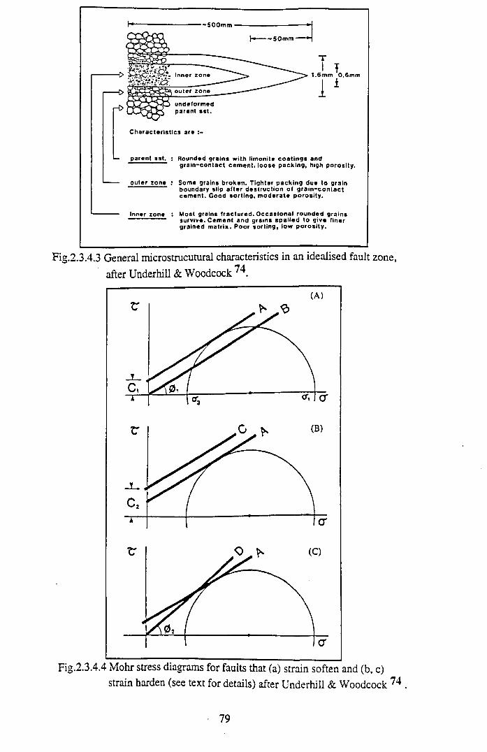
1.6mm 0.6mmi

Characteristics are : -

parent sst. : Rounded grains with limonite coatings andgrain-contact cement, loose packing, high porosity.

outer zone ; Some grains broken. Tighter packing due to grain boundary slip after destruction of grain-contact cement. Good sorting, moderate porosity.

Inner zone : Most grains fractured. Occasional rounded grains ' survive. Cement and grains spalled to give finer

grained matrix. Poor sorting, low porosity.

Fig.2.3.4.3 General microstrucutural characteristics in an idealised fault zone, after Underhill & Woodcock 74.

Fig.2.3.4.4 Mohr stress diagrams for faults that (a) strain soften and (b, c)strain harden (see text for details) after Underhill & Woodcock 74 .

79

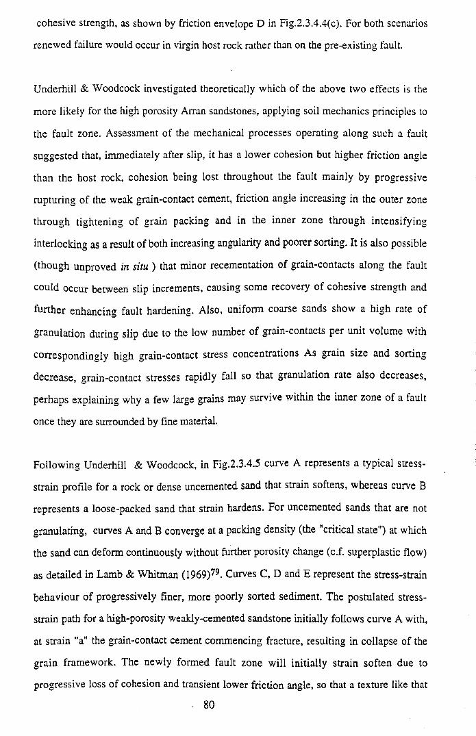
cohesive strength, as shown by friction envelope D in Fig.2.3.4.4(c). For both scenarios

renewed failure would occur in virgin host rock rather than on the pre-existing fault.

Underhill & Woodcock investigated theoretically which of the above two effects is the

more likely for the high porosity Arran sandstones, applying soil mechanics principles to

the fault zone. Assessment of the mechanical processes operating along such a fault

suggested that, immediately after slip, it has a lower cohesion but higher friction angle

than the host rock, cohesion being lost throughout the fault mainly by progressive

rupturing of the weak grain-contact cement, friction angle increasing in the outer zone

through tightening of grain packing and in the inner zone through intensifying

interlocking as a result of both increasing angularity and poorer sorting. It is also possible

(though unproved in situ ) that minor recementation of grain-contacts along the fault

could occur between slip increments, causing some recovery of cohesive strength and

further enhancing fault hardening. Also, uniform coarse sands show a high rate of

granulation during slip due to the low number of grain-contacts per unit volume with

correspondingly high grain-contact stress concentrations As grain size and sorting

decrease, grain-contact stresses rapidly fall so that granulation rate also decreases,

perhaps explaining why a few large grains may survive within the inner zone of a fault

once they are surrounded by fine material.

Following Underhill & Woodcock, in Fig.2.3.4.5 curve A represents a typical stress-

strain profile for a rock or dense uncemented sand that strain softens, whereas curve B

represents a loose-packed sand that strain hardens. For uncemented sands that are not

granulating, curves A and B converge at a packing density (the "critical state") at which

the sand can deform continuously without further porosity change (c.f. superplastic flow)

as detailed in Lamb & Whitman (1969)79. Curves C, D and E represent the stress-strain

behaviour of progressively finer, more poorly sorted sediment. The postulated stress-

strain path for a high-porosity weakly-cemented sandstone initially follows curve A with,

at strain "a" the grain-contact cement commencing fracture, resulting in collapse of the

grain framework. The newly formed fault zone will initially strain soften due to

progressive loss of cohesion and transient lower friction angle, so that a texture like that

80

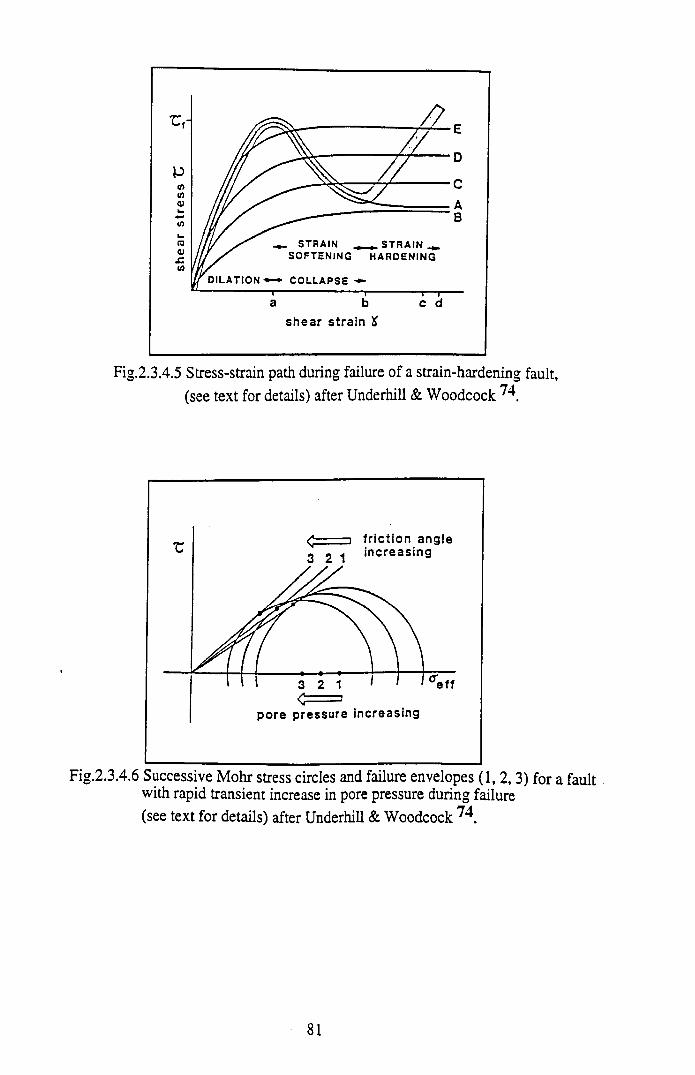
Fig.2.3.4.5 Stress-strain path during failure of a strain-hardening fault, (see text for details) after Underhill & Woodcock

Fig.2.3.4.6 Successive Mohr stress circles and failure envelopes (1, 2 ,3) for a fault . with rapid transient increase in pore pressure during failure(see text for details) after Underhill & Woodcock

81

of the outer fault zone (Fig.2.3.4.3) develops. The fault is postulated to behave as though

it were an uncemented sand so that its deformation path would follow curve A, were it

not for the depth of burial being sufficient for ambient stress magnitudes to induce grain

fracture. In this case, when the grain framework can collapse no further (at strain "b")

grains start to fracture, initially at a high rate but decreasing as grain-size decreases.

Friction angle increases and the stress-strain path is driven up again by the strain

hardening effect, crossing curves C, D and E at a strain appropriate to the grain-size at the

time. Finally, the fault zone locks at strain "d" as it strain hardens to a point at which its

frictional resistance exceeds the shear stress along it.

An obvious problem with this stress-strain path, as noted by Underhill & Woodcock, is

that the locked-up stress must exceed the initial failure stress, (Tf in Fig.2.3.4.5) if net

strain hardening has occurred. Two possible explanations were proposed. The first is that

stress overshoot does not in fact occur, the fault locking up when the frictional resistance

reaches the initial host rock failure (fracture) stress at strain "c". The second is that

apparent stress overshoot occurs because of transient pore pressure increase along the

fault. In the latter case, it is possible for the shear stress on the fault to remain constant or

even to decrease, but still promote slip due to the effective normal stress being lowered

by the increasing pore pressure. On a Mohr circle plot (Fig.2.3.4.6) this situation can be

represented by successive stress circles being driven to the left to track a series of failure

envelopes with increasing friction angle. After failure, the excess pore pressure dissipates

and the stress circle moves to the right, well away from the failure envelopes. Whilst

long-term abnormal pore pressures seem unlikely in these porous and permeable

sandstones, transient high pore pressures along the faults seem likely during slip. Pore

fluid has to escape from both the outer and inner zones of the fault as porosity decreases,

its escape being progressively slowed, especially in the inner zone, by decreasing

permeability, suggesting transient overpressuring of the fault zone as a plausible cause of

apparent stress overshoot.

Aydin & Johnson (1983)*^ also studied the mechanisms and mechanics of faulting in

porous rocks, in terms of a theory of deformation of elasto-plastic, time-independent

82

materials developed in a series of papers by Rice, Rudnicki and Cleary (Rice, 197581,

Rudnicki & Rice. 197582, Cleary & Rudnicki, 197683, Cleary, 197684, Rudnicki, 197785,

Rice, 197986) and by Eshelby (1957)87, which generalised plasticity theory such that it

can describe localised deformation in idealised plastic or brittle materials. The tendency

for strain to localise in porous rocks can be understood in terms of "bifurcation" in the

macroscopic constitutive relations (see for example Vardoulakis et al, 198088).

Mathematically speaking, here "bifurcation" refers to loss of uniqueness of the boundary

solution as a result of considering the shear band as a zone in which there is localisation

o f strain leading to a macroscopic instability of the material. Aydin & Johnson80

observed that slip surfaces in the Entrada and Navajo sandstones occurred within well-

developed zones of deformation bands, representing extremely localised, large

deformation. They interpreted the formation of such slip surfaces in terms of instability

represented by Rudnicki's85 "runaway instability" and by Rice's86 "Eshelby line"

describing interaction between the inelastic properties of the material, in this case the

fault zone, and the "softness" of the loading system, in this case the matrix. In effect, the

relatively soft matrix behaves much as a "soft" loading machine used in testing rocks in

which a rock specimen (analogous to the fault material) fails violently as strain energy is

released from the loading machine. As the material within a fault zone is stiffer than the

surrounding sandstone matrix, as described by Underhill & Woodcock74, the stresses

within the zone are higher than the far-field stresses, so that the surrounding sandstone

can be deforming elastically under relatively low far-field stresses, whereas the stresses

within the zone can be sufficiently high for the strains to become extremely large, field

observation by Aydin & Johnson80 showing these large strains being accommodated

along a discrete surface or discontinuity.

A comprehensive summary of production-related properties o f granulation seams

(specifically permeability and porosity reduction) is given by Kulander et al (1990)75.

The concept of permeability reduction in a fault zone is based on a limited set of

permeability measurements (Pittman, 198171, Harper & Moftah, 198589, Nelson, 198590)

made perpendicular and parallel to a gouge zone in sandstone, indicating dramatic

83

variation in percentage reduction of gouge zone compared to matrix permeability, both

within an individual formation (11 to 95%) and between formations (11 to 99%). Such

wide variations in the percentage of permeability reduction is almost certainly a function

of varying host rock composition, grain size and porosity, combined with variations in the

degree of granulation involved. Apparent porosity reductions as observed in thin-section

have been reported frequently (Aydin70, Pittman71, Jamison & Stearns, 198272,

Nelson90, Underhill & Woodcock74) however due to the very small grain-sizes involved,

estimates of porosity from thin-section point-counting techniques should be treated with

caution. Aydin70 used a statistical approach to determine the average porosity reduction

in a series of gouge zones in sandstone. By calculating the difference in the average

porosity of two populations of plugs, one with and one without gouge zones, the average

porosity reduction associated with granulation of the host rock was determined at around

60 to 75%. As an alternative to thin-section analysis and the Aydin statistical approach,

Kulander et al 75 examined the porosity reduction in a more rigorous manner through

Computerised Axial Tomography (CAT) scanning techniques, and found an average

porosity reduction of 46% for a whole core sample with a single inclined granulation

seam.

2.3.5 Fault Seal Capacity In the North Sea

The majority of North Sea structural traps require that at least one fault be a sealing fault.

The typical trap in the North Sea is a tilted fault block with at least one fault sealing the

hydrocarbon column. Faults can act as pressure barriers to subsurface fluids during the

production life of a field or as differential migration barriers to hydrocarbons over

geological time, so that an understanding of the probability of a fault acting as a

differential migration barrier is critical for prospects relying on fault seal. The probability

of a fault acting as a pressure barrier is important in field development and production

where fault bounded compartments may not be in pressure communication because of

sealing faults. Knott47 examined over 400 faults from 101 exploration targets and 25 oil

and gas fields in a regional study of fault seal in the North Sea. The faults cut clastic

successions from a variety of depositional environments (marine, paralic and nonmarine)

from both Brent Group and Rotliegendes Group stratigraphies. The emphasis of the study

84

was on fault-related seals that act as pressure or migration barriers over geological time,

with one of the objectives being the determination of those parameters most important in

controlling fault seals, especially where reservoir is juxtaposed against reservoir

(empirical understanding of such controls is a prerequisite for fault seal prediction).

Knott classified fault related seals according to the following definitions (Fig.2.3.5.1):

(i) Juxtaposition fault. The fault forms an essential trapping element to an isolated

hydrocarbon accumulation and sealing occurs due to abutment of the reservoir

lithology against a sealing lithology

(ii) Partially sealing fault. The fault separates reservoir compartments with different

hydrocarbon-water contacts in a single pool with no pressure drawdown between

adjacent compartments during the production life of the field and over a range of

pressure intervals

(iii) Temporary sealing fault. The fault may act as a temporary pressure barrier during

production but not over geologic time, therefore no initial change occurs in elevation

of the hydrocarbon water contact across the fault

For partially sealing faults, seal is provided mainly by the fault plane itself, due to, for

instance, mechanical and chemical reduction of porosity and permeability of the reservoir

rock within the fault zone, although a component of juxtaposition seal may also be

present. For temporary sealing faults, seal may occur across the upper part of the fault

due to juxtaposition and across the remainder of the fault by a combination of

juxtaposition and membrane seal (the capacity of the latter in this case being insufficient

to support differential hydrocarbon column heights across the fault over geological time).

Knott analysed only the fault-related seals within classes (i) and (ii) as above, that is those

faults (juxtaposition and partially-sealing) sealing over geological time, as primary

interest lay in determination of those parameters controlling fault seal in exploration

targets, and in faulted segments of fields with different hydrocarbon/water contacts

(although some of the observations may well be applicable to temporary sealing faults).

85

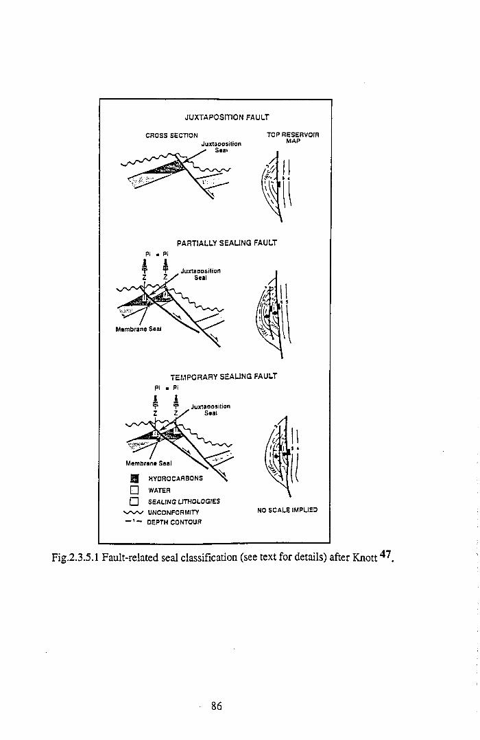
J U X T A P O S IT IO N F A U L T

PARTIALLY SEALING FAULTPi « Pi

TEMPORARY SEALING FAULT Pi ■ Pi

□ SEALING LITHOLOGIESUNCONFORMITY

— DEPTH CONTOUR

Fig.2.3.5.1 Fault-related seal classification (see text for details) after Knott ^ .

86

In Knott's analysis, a fault was determined to be sealing sensu stricto (that is membrane

sealing along the fault plane) from pressure data, geochemistry, hydrocarbon type,

hydrocarbon-water contacts and production data where available. The importance of

differentiating between geometries and mechanisms was also stressed, for example whilst

a juxtaposition fault is a geometrical effect which may seal by that mechanism, the actual

sealing may be provided by, for example, clay smear. A purely geometric subdivision

was also employed, based on the relation between fault throw and reservoir interval

thickness:

(i) Extrareservoir fault. A fault which completely offsets the reservoir interval against a

sealing lithology

(ii) Intrareservoir fault. A fault which only partly offsets the reservoir interval, or throws

one reservoir interval against another

Whilst the sealing mechanism in the former is generally by juxtaposition, in the latter the

sealing mechanism can be either membrane seal (clay smear, cataclasis, or cementation

along the fault plane) or juxtaposition. This geometric definition was deemed necessary

because the North Sea reservoirs under consideration (Brent Group and Rotliegendes

Group) are generally overlain and underlain by sealing lithologies at least as thick as the

reservoir intervals, so that a useful first-order distinction exists where extrareservoir faults

are more likely to provide juxtaposition seal than intrareservoir faults. Knott recognised

the following parameters as important contributors to fault seal (see Fig.2.3.5.2):

(i) Fault orientation. Fault trend may influence sealing, for example in strike-slip

systems reverse faults are considered more likely to seal than normal faults due to

greater shear stress for fault displacement in the former

(ii) Burial depth. With increasing confining pressure, faulting mechanisms favourable to

fault seal (such as cataclasis) are more pronounced, also diagenetic reactions that

reduce porosity and permeability also increase with depth (however sealing due to

clay smear is more likely at shallow depths where mud is undercompacted

87

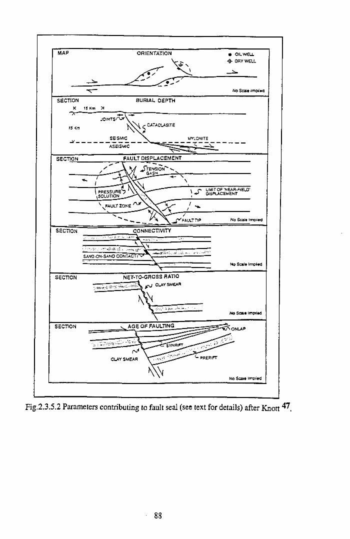
Fig.2.3.5.2 Parameters contributing to fault seal (see text for details) after Knott ^ .

88

(iii) Fault displacement. For a particular lithology the larger the fault throw the wider the

fault zone and the greater the mechanical reduction in porosity and permeability due

to cataclasis. With varying fault displacement, zones of extension (tension gashes)

and contraction (pressure solution) form, with fault seal being less likely in zones

where open fractures are present

(iv) Net-to-gross ratio (N/G). Defined as the thickness of the net reservoir divided by the

overall thickness of the interval in question, the percentage and distribution of

nonreservoir rocks in a succession indicates the likelihood of ductile smear or

injection (membrane seal) of these lithologies along the fault zone. The N/G also

indicates the probability that there are sandstone to sandstone contacts across the

fault (not necessarily of the same unit)

(v) Connectivity. Juxtaposition of reservoir against nonreservoir across a fault produces a

juxtaposition seal. Defined by Knott as, "the fraction of net sand in the reservoir

interval in geometric contact across the fault" a complete analysis of the role of

connectivity requires an accurate picture of the stratigraphy on either side of the fault

for its entire length. Sand-on-sand contacts across faults where there is no membrane

seal or clay smear are unlikely to provide seal

(vi) Age of faulting. Syndepositional faulting usually favours membrane sealing as muds

are generally undercompacted, exhibiting greater ductility, and are therefore more

likely to smear than shales in pre-rift sections which are more likely to be indurated

(hardened)

Knott plotted parameters including fault strike and throw, reservoir thickness and depth,

N/G, porosity and net sand connectivity against seal performance to define trends and

correlations to predict fault seal characteristics. In summary, a correlation was evident

(although not statistically significant) between fault orientation and sealing, sealing was

found proportional to fault throw normalised as a fraction of the reservoir thickness, and

the great majority of faults with throws greater than the thickness of the reservoir interval

were sealing faults. Knott concluded that the most useful parameters in fault seal

prediction are fault displacement, N/G and net sand connectivity.

89

2.4 DEFORM ABILITY

In an assessment of the effects of shear discontinuities in the hydrocarbon reservoir

environment, fault population statistics (section 2 .2 ) and sealing potential (section 2 .3 )

have been discussed in terms of their relative influence on hydrocarbon structural

entrapment and pore fluid migration. However, whilst the above effects represent (with

the exception of the seismic pumping/valving phenomena) largely "passive" controls on

fluid flow, current rock mechanics philosophy also predicts a "reactive" role for shear

discontinuities, due to the response of pre-existing fractures and indeed the formation of

new fractures resulting from transients in the in situ stress field associated with

production. In section 2.4 the role of shear discontinuities in controlling overall reservoir

deformation resulting from temporal variations in specifically pore fluid pressure are

assessed. In section 2.4.1 the phenomenon of reservoir seismicity due to induced fault

formation and reactivation is discussed, whilst in section 2.4.2 induced shear slippage on

planes of sedimentary heterogeneity, as an important contributing mechanism for strain

accommodation within a deforming reservoir, is reviewed.

2.4.1 Production-related Seismicity

In recent years it has become increasingly apparent that some of man's engineering

activities can have a measurable influence on the way in which crustal stresses are

released in earthquakes. Increases in seismic activity have resulted from: impoundment of

reservoirs behind high dams; large-scale surface quarrying; deep underground mining; the

injection of fluids under high pressure into the ground in solution mining, waste disposal,

geothermal power generation, and secondary oil recovery; the removal o f fluids in

hydrocarbon recovery; the after-effects of large underground explosions. A number of

adjectives have been used to describe this type of seismicity - "man-made", "induced",

"artificial" and "triggered".

Engineering works can influence the in situ stress regime through changes in solid

(elastic) stress or fluid (pore) pressure. The orientation of the principal stresses in nature

varies with the tectonic environment, with the minimum principal stress, <33 , vertical in

90

regions of thrust faulting, the maximum principal stress, <7|, vertical in regions of normal

faulting and the intermediate principal stress, <72, vertical in regions of strike-slip

faulting, so that the triggering effect of the induced elastic stress will be greatest in

regions where the induced stress adds to the tectonic shear stress by increasing the radius

of the Mohr circle representing CTi and <73, either by increasing <Ji or decreasing <73. Thus

an increase in vertical stress from the elastic load of a dam impounded reservoir will have

the greatest impact in regions of normal faulting where the vertical stress is the

maximum, whereas a decrease in vertical stress due to the removal of surface load in

quarrying operations will have the greatest impact in regions of thrust faulting, where the

vertical stress is the minimum. Increasing pore pressure (for example by fluid injection)

whilst not changing the radius of the Mohr stress circle, translates the circle to the left on

a M ohr diagram, and thus always moves the circle towards the failure envelope,

regardless of the tectonic stress environment.

In terms of this simple representation of failure, earthquakes are triggered when one of

the following situations occurs (Simpson, 198691): (i) the pre-existing stress conditions

on a fault are such that the magnitude of the induced stresses are sufficient to produce

failure; (ii) the triggering source acts to drive the natural stress condition closer to the

failure envelope either (a) by a purely elastic effect increasing the differential stress

(increasing the diameter of the Mohr circle) or (b) through increased pore pressure,

decreasing the effective stress (translating the Mohr circle towards the failure envelope)

or (c) a combined elastic and pore pressure effect. In Fig.2.4.1.1, comparison is made

between the influence of isolated changes in elastic stress decrease (a) for mining and

increase (b) for "dry" reservoir impoundment (zero pore pressure effects), isolated

changes in pore pressure (c) for fluid injection, and combined elastic and pore pressure

effects (d) for "wet" reservoir impoundment (significant pore pressure effects).

W ith regard to hydrocarbon reservoirs, very few oilfields have been monitored by

standard microseismic techniques, but of those which have, there is substantial evidence

of induced fracturing. This takes the form of microearthquakes of magnitude, M>3 on the

local Richter scale, corresponding to slip on faults up to a scale of a few hundred metres,

91

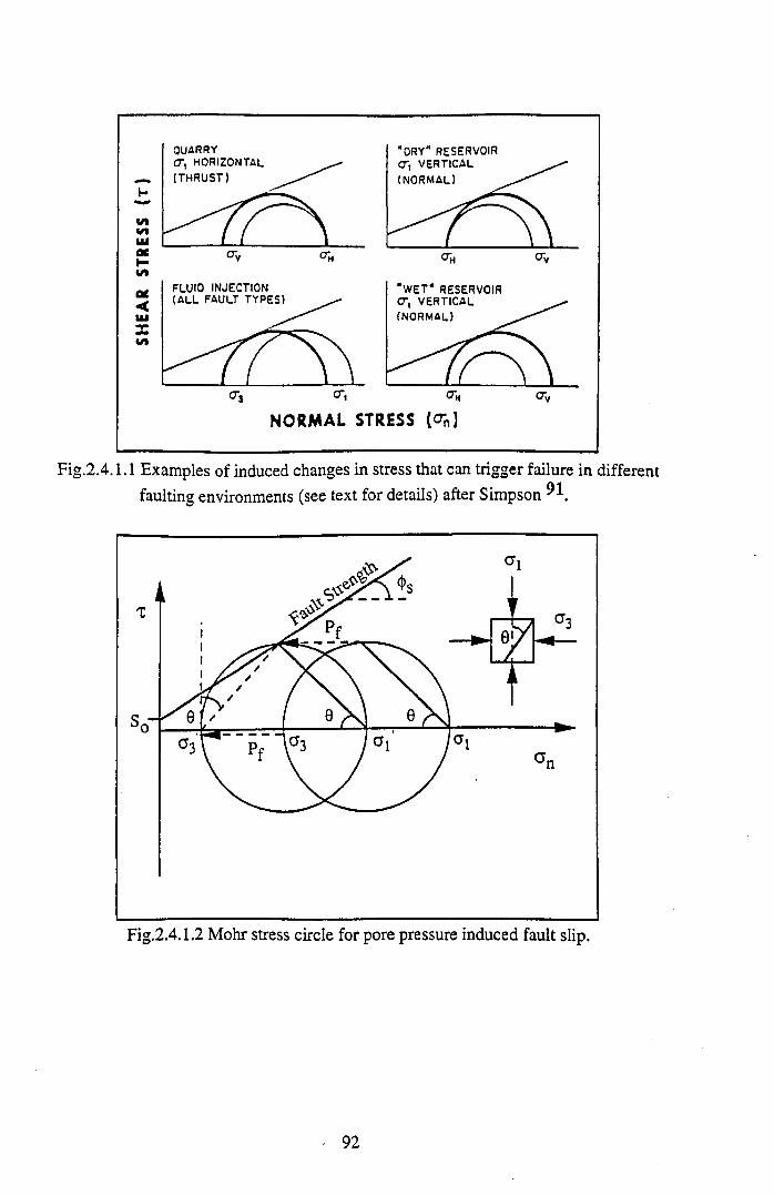
Fig.2.4.1.1 Examples of induced changes in stress that can trigger failure in different faulting environments (see text for details) after Simpson ^1.

Fig.2.4.1.2 Mohr stress circle for pore pressure induced fault slip.

92

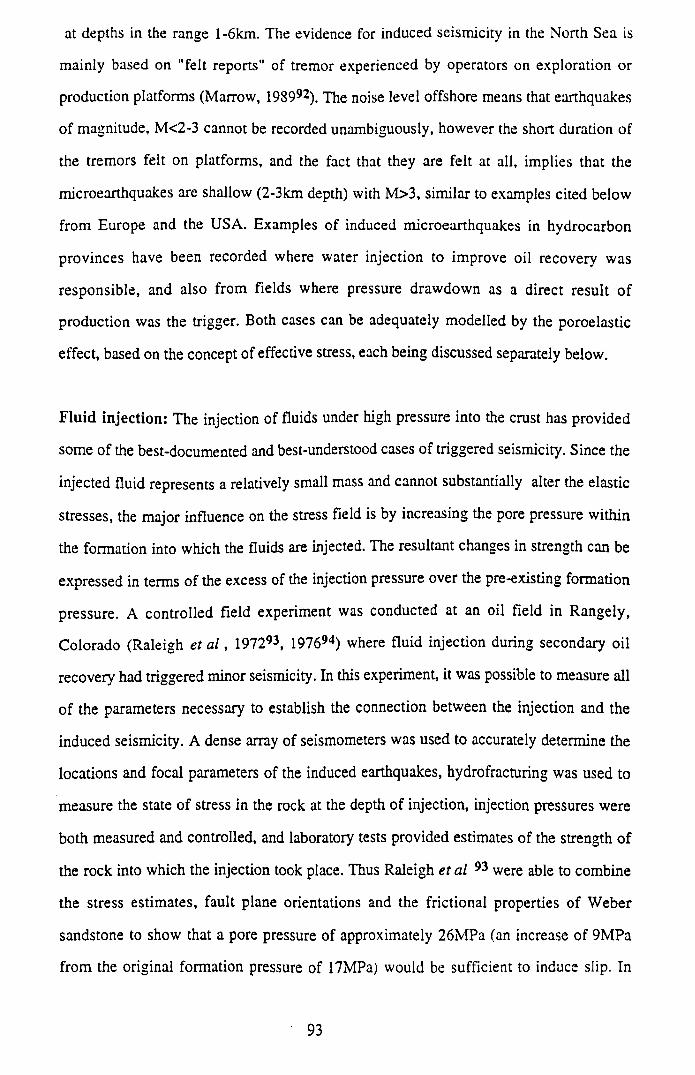
at depths in the range l - 6km. The evidence for induced seismicity in the North Sea is

mainly based on "felt reports" of tremor experienced by operators on exploration or

production platforms (Marrow, 198992). The noise level offshore means that earthquakes

of magnitude, M<2-3 cannot be recorded unambiguously, however the short duration of

the tremors felt on platforms, and the fact that they are felt at all, implies that the

microearthquakes are shallow (2-3km depth) with M>3, similar to examples cited below

from Europe and the USA. Examples of induced microearthquakes in hydrocarbon

provinces have been recorded where water injection to improve oil recovery was

responsible, and also from fields where pressure drawdown as a direct result of

production was the trigger. Both cases can be adequately modelled by the poroelastic

effect, based on the concept of effective stress, each being discussed separately below.

Fluid injection: The injection of fluids under high pressure into the crust has provided

some of the best-documented and best-understood cases of triggered seismicity. Since the

injected fluid represents a relatively small mass and cannot substantially alter the elastic

stresses, the major influence on the stress field is by increasing the pore pressure within

the formation into which the fluids are injected. The resultant changes in strength can be

expressed in terms of the excess of the injection pressure over the pre-existing formation

pressure. A controlled field experiment was conducted at an oil field in Rangely,

Colorado (Raleigh et a l , 197293, 197694) where fluid injection during secondary oil

recovery had triggered minor seismicity. In this experiment, it was possible to measure all

of the parameters necessary to establish the connection between the injection and the

induced seismicity. A dense array of seismometers was used to accurately determine the

locations and focal parameters of the induced earthquakes, hydrofracturing was used to

measure the state of stress in the rock at the depth of injection, injection pressures were

both measured and controlled, and laboratory tests provided estimates of the strength of

the rock into which the injection took place. Thus Raleigh et al 93 were able to combine

the stress estimates, fault plane orientations and the frictional properties of Weber

sandstone to show that a pore pressure of approximately 26MPa (an increase of 9MPa

from the original formation pressure of 17MPa) would be sufficient to induce slip. In

93

Raleigh et al 94, seismicity was shown to be controllable by raising and lowering the

pore pressure about the predicted value of 26MPa.

Shear fractures obey the effective stress principle in that internal fluid pore pressure

within the fracture directly counteracts the strengthening effect of the external normal

stress applied across the slip plane. To calculate the fluid pressure required to cause a

fault or joint to slip, it is necessary to quantify the amount by which the M ohr circle

corresponding to the current state of stress has to travel to the left to bring the normal and

shear stress on the fault plane to the limiting condition represented by the criterion of

failure (Fig.2.4.1.2). This calculation is slightly more complicated than for the case of

unfractured rock, because in addition to initial stresses and strength parameters, the

orientation of the fault plane (9 with respect to the ai-direction) needs to be considered.

If the initial stresses are C3 and 0 1 , then the pore fluid pressure, Pf, that will produce fault

slip is (Goodman, 198995):

From Eqn.2.4.1.1 it is evident that initial crustal stresses, fault orientation and frictional

strength properties of the fault plane (cohesion, S0, and angle of sliding friction, 0 S) are

required in order to predict the likelihood of triggering earthquakes from fluid injection.

This simple application of the effective stress principal has been shown to satisfactorily

explain the occurrence of earthquakes due to water injection in a deep waste disposal well

near Denver, Colorado (Healy et al, 196896) and in the Rangely oilfield, western

Colorado (Raleigh et al 93*94).

Davis & Penington (1989)97 examined a sequence of induced earthquakes that occurred

at the Codgell oil field, West Texas, from about 1974 to 1982. The earthquakes occurred

within an array of injecting wells which surrounded the perimeter of the field and which

decreased in radius during the life of the injection project. Whilst from the above

Eqn.2.4.1.1

94

discussion (Eqn.2.4.1.1) it is evident that significant increases in field fluid pressures due

to injection can result in the occurrence of significant triggered earthquakes (the largest of

the Denver earthquakes exceeded M>5) Davis & Penington noted that, however, high

fluid pressures do not necessarily result in earthquakes, pointing out that numerous

examples of injection sites were present in Texas where induced failure should have

occurred by any reasonable failure law, but that no earthquakes had been observed. Thus,

although the lowering of effective rock strength from injection is clearly the predominant

mechanism controlling failure in many sites, other mechanisms may also contribute. In

particular, they highlighted the mechanism whereby slip along one section of a fault may

load stress onto nearby locked portions of a fault, a process considered significant for

major plate boundary faults, but generally overlooked as a cause of small-scale intraplate

triggered earthquakes. They examined the sequence of earthquakes recorded at Codgell in

terms of two failure models. In the first model, seismic failure occurred when and where

fluid pressures exceeded some critical value as given by Eqn.2.4.1.1. In the second

model, earthquakes occurred at the edges of low fluid pressure areas where stresses had

been transferred as a result of aseismic deformation in adjacent high fluid pressure

regions.

Fluid pressures may affect the behaviour of faults in two ways:

(i) Increase in pore pressure lowers the effective strength of faults (Hubbert & Rubey,

195998)

(ii) Increase in pore pressure can alter the mode of deformation from seismic stick-slip to

aseismic creep (Byerlee & Brace, 1972")

From Eqn.2.4.1.1, for the Codgell oil field with S0 = 4MPa, ¡j.s = 0.8 (<j>s = 39°), Ci =

47MPa and <53 = 28MPa, Davis & Penington" calculated that an injection pressure of Pf

= 6MPa should be sufficient to induce failure, however injection pressures at Codgell had

exceeded 38MPa since 1960, and indeed, for these values, 877 of the 2420 projects in

Texas which injected at shallow depths should be in failure, whereas only the Codgell

95

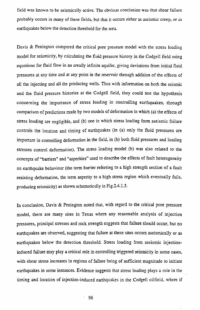
field was known to be seismically active. The obvious conclusion was that shear failure

probably occurs in many of these fields, but that it occurs either as aseismic creep, or as

earthquakes below the detection threshold for the area.

Davis & Penington compared the critical pore pressure model with the stress loading

model for seismicity, by calculating the fluid pressure history in the Codgell field using

equations for fluid flow in an areally infinite aquifer, giving deviations from initial fluid

pressures at any time and at any point in the reservoir through addition of the effects of

all the injecting and all the producing wells. Thus with information on both the seismic

and the fluid pressure histories at the Codgell field, they could test the hypothesis

concerning the importance o f stress loading in controlling earthquakes, through

comparison o f predictions made by two models of deformation in which (a) the effects of

stress loading are negligible, and (b) one in which stress loading from aseismic failure

controls the location and timing of earthquakes (in (a) only the fluid pressures are

important in controlling deformation in the field, in (b) both fluid pressures and loading

stresses control deformation). The stress loading model (b) was also related to the

concepts of “barriers” and “asperities” used to describe the effects of fault heterogeneity

on earthquake behaviour (the term barrier referring to a high strength section of a fault

resisting deformation, the term asperity to a high stress region which eventually fails,

producing seismicity) as shown schematically in Fig.2.4.1.3.

In conclusion, Davis & Penington noted that, with regard to the critical pore pressure

model, there are many sites in Texas where any reasonable analysis o f injection

pressures, principal stresses and rock strength suggests that failure should occur, but no

earthquakes are observed, suggesting that failure at these sites occurs aseismically or as

earthquakes below the detection threshold. Stress loading from aseismic injection-

induced failure may play a critical role in controlling triggered seismicity in some cases,

with shear stress increases in regions of failure being of sufficient magnitude to initiate

earthquakes in some instances. Evidence suggests that stress loading plays a role in the

timing and location of injection-induced earthquakes in the Codgell oilfield, where if

96

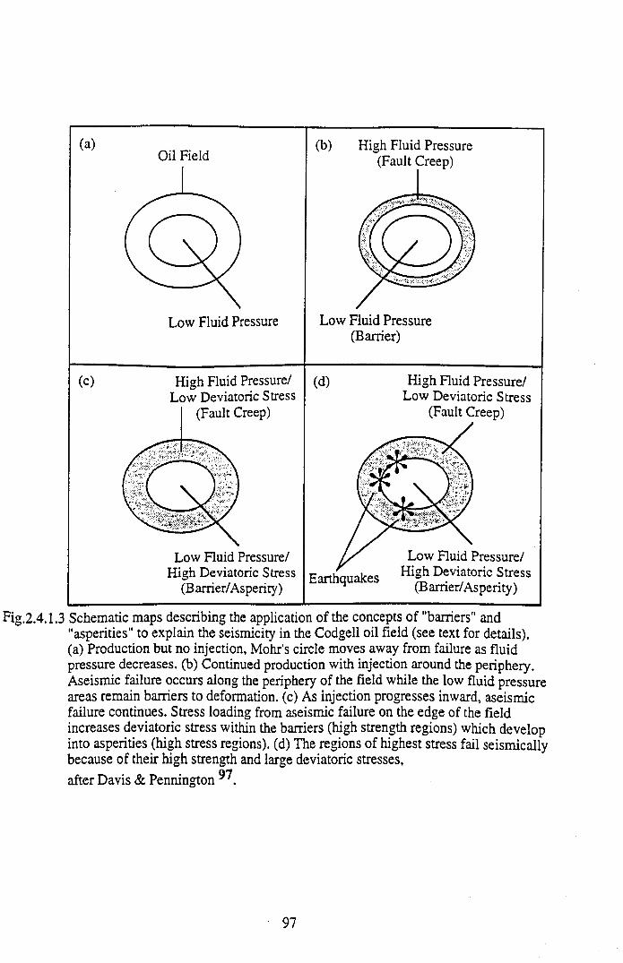
Fig.2.4.1.3 Schematic maps describing the application of the concepts of "barriers'1 and"asperities" to explain the seismicity in the Codgell oil field (see text for details).(a) Production but no injection, Mohr's circle moves away from failure as fluid pressure decreases, (b) Continued production with injection around the periphery. Aseismic failure occurs along the periphery of the field while the low fluid pressure areas remain barriers to deformation, (c) As injection progresses inward, aseismic failure continues. Stress loading from aseismic failure on the edge of the field increases deviatoric stress within the barriers (high strength regions) which develop into asperities (high stress regions), (d) The regions of highest stress fail seismically because of their high strength and large deviatoric stresses,after Davis & Pennington

97

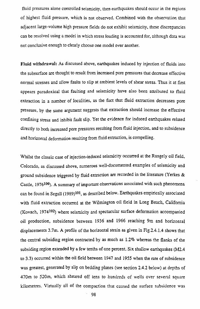
fluid pressures alone controlled seismicity, then earthquakes should occur in the regions

of highest fluid pressure, which is not observed. Combined with the observation that

adjacent large-volume high pressure fields do not exhibit seismicity, these discrepancies

can be resolved using a model in which stress loading is accounted for, although data was

not conclusive enough to clearly choose one model over another.

F luid w ithdraw al: As discussed above, earthquakes induced by injection of fluids into

the subsurface are thought to result from increased pore pressures that decrease effective

normal stresses and allow faults to slip at ambient levels of shear stress. Thus it at first

appears paradoxical that faulting and seismicity have also been attributed to fluid

extraction in a number of localities, as the fact that fluid extraction decreases pore

pressure, by the same argument suggests that extraction should increase the effective

confining stress and inhibit fault slip. Yet the evidence for induced earthquakes related

directly to both increased pore pressures resulting from fluid injection, and to subsidence

and horizontal deformation resulting from fluid extraction, is compelling.

Whilst the classic case of injection-induced seismicity occurred at the Rangely oil field,

Colorado, as discussed above, numerous well-documented examples of seismicity and

ground subsidence triggered by fluid extraction are recorded in the literature (Yerkes &

Castle, 1976^00). A. summary of important observations associated with such phenomena

can be found in Segall (1989)101, as described below. Earthquakes empirically associated

with fluid extraction occurred at the Wilmington oil field in Long Beach, California

(Kovach, 1974102) where seismicity and spectacular surface deformation accompanied

oil production, subsidence between 1936 and 1966 reaching 9m and horizontal

displacements 3.7m. A profile of the horizontal strain as given in Fig.2.4.1.4 shows that

the central subsiding region contracted by as much as 1.2 % whereas the flanks of the

subsiding region extended by a few tenths of one percent. Six shallow earthquakes (M2.4

to 3.3) occurred within the oil field between 1947 and 1955 when the rate of subsidence

was greatest, generated by slip on bedding planes (see section 2.4.2 below) at depths of

470m to 520m, which sheared off tens to hundreds o f wells over several square

kilometres. Virtually all of the compaction that caused the surface subsidence was

98

Fig-2.4.1.4 Measured surface deformations at Wilmington oil field near Long Beach, California (a) Horizontal strain change, (b) radial displacement (inward +ve.) between 1937 and 1962, and vertical displacement (downward -ve.) between 1928 and 1962. Note limits of producing zone and location of bedding plane faults,

after Segall

Fig.2.4.1.5 Number of earthquakes recorded per year and decline in averagereservoir pressure in two gas fields, (a) Strachan oil field in Alberta,Canada, (b) Pau basin gas field, France, after Segall

99

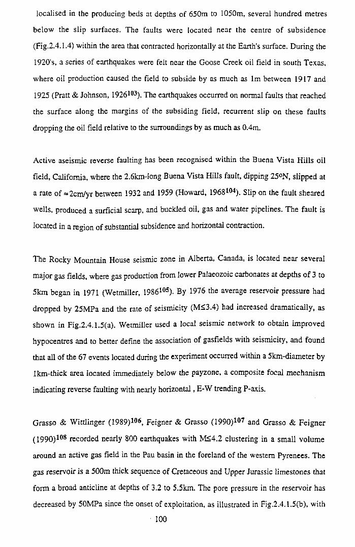
localised in the producing beds at depths of 650m to 1050m, several hundred metres

below the slip surfaces. The faults were located near the centre of subsidence

(Fig.2.4.1.4) within the area that contracted horizontally at the Earth's surface. During the

1920's, a series of earthquakes were felt near the Goose Creek oil field in south Texas,

where oil production caused the field to subside by as much as lm between 1917 and

1925 (Pratt & Johnson, 1926103). The earthquakes occurred on normal faults that reached

the surface along the margins of the subsiding field, recurrent slip on these faults

dropping the oil field relative to the surroundings by as much as 0.4m.

Active aseismic reverse faulting has been recognised within the Buena Vista Hills oil

field, California, where the 2 .6km-Iong Buena Vista Hills fault, dipping 25°N, slipped at

a rate of «2cm /yr between 1932 and 1959 (Howard, 1968104). Slip on the fault sheared

wells, produced a surficial scarp, and buckled oil, gas and water pipelines. The fault is

located in a region of substantial subsidence and horizontal contraction.

The Rocky Mountain House seismic zone in Alberta, Canada, is located near several

major gas fields, where gas production from lower Palaeozoic carbonates at depths o f 3 to

5km began in 1971 (Wetmiller, 1986105). By 1976 the average reservoir pressure had

dropped by 25MPa and the rate of seismicity (M<3.4) had increased dramatically, as

shown in Fig.2.4.1.5(a). Wetmiller used a local seismic network to obtain improved

hypocentres and to better define the association of gasfields with seismicity, and found

that all of the 67 events located during the experiment occurred within a 5km-diameter by

lkm -thick area located immediately below the payzone, a composite focal mechanism

indicating reverse faulting with nearly horizontal, E-W trending P-axis.

Grasso & W ittlinger (1989)106, Feigner & Grasso (1990)107 and Grasso & Feigner

(1990)108 recorded nearly 800 earthquakes with M<4.2 clustering in a small volume

around an active gas field in the Pau basin in the foreland of the western Pyrenees. The

gas reservoir is a 500m thick sequence of Cretaceous and Upper Jurassic limestones that

form a broad anticline at depths of 3.2 to 5.5km. The pore pressure in the reservoir has

decreased by 50MPa since the onset of exploitation, as illustrated in Fig.2.4.1.5(b), with

1 0 0

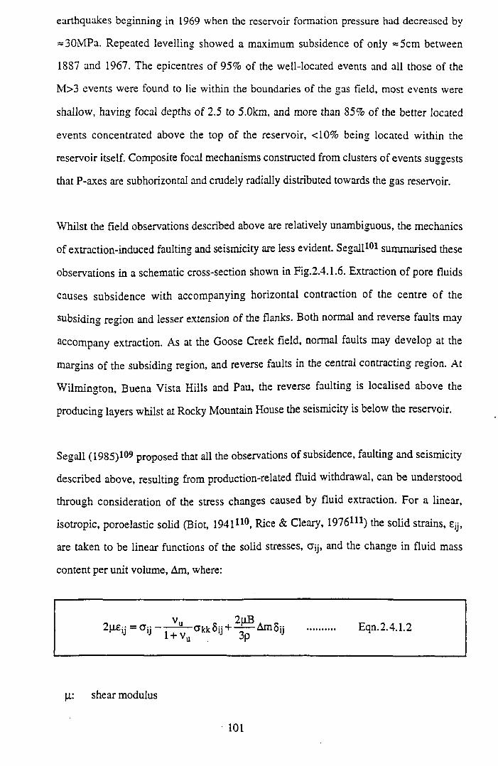
earthquakes beginning in 1969 when the reservoir formation pressure had decreased by

= 30MPa. Repeated levelling showed a maximum subsidence of only = 5cm between

1887 and 1967. The epicentres of 95% of the well-located events and ail those of the

M>3 events were found to lie within the boundaries of the gas field, most events were

shallow, having focal depths of 2.5 to 5.0km, and more than 85% of the better located

events concentrated above the top of the reservoir, < 10% being located within the

reservoir itself. Composite focal mechanisms constructed from clusters of events suggests

that P-axes are subhorizontal and crudely radially distributed towards the gas reservoir.

Whilst the field observations described above are relatively unambiguous, the mechanics

of extraction-induced faulting and seismicity are less evident. Segall101 summarised these

observations in a schematic cross-section shown in Fig.2.4.1.6. Extraction o f pore fluids

causes subsidence with accompanying horizontal contraction of the centre of the

subsiding region and lesser extension of the flanks. Both normal and reverse faults may

accompany extraction. As at the Goose Creek field, normal faults may develop at the

margins of the subsiding region, and reverse faults in the central contracting region. At

Wilmington, Buena Vista Hills and Pau, the reverse faulting is localised above the

producing layers whilst at Rocky Mountain House the seismicity is below the reservoir.

Segall (1985)109 proposed that all the observations of subsidence, faulting and seismicity

described above, resulting from production-related fluid withdrawal, can be understood

through consideration of the stress changes caused by fluid extraction. For a linear,

isotropic, poroelastic solid (Biot, 1941*10, Rice & Cleary, 1976***) the solid strains, £y,

are taken to be linear functions of the solid stresses, ay , and the change in fluid mass

content per unit volume, Am, where:

2(I£ij = Ojj -U - ^ u- a kkSii + — Ants»l + v u “ 1J 3p 1J

Eqn.2.4.1.2

|i: shear modulus

Fig.2.4.1.6 Schematic cross-section summarising surface deformation and faulting associated with fluid withdrawal (open arrows indicate horizontal strainat earth's surface) after Segall

Fig.2.4.1.7 Calculated change in horizontal normal stress, Gyy, due to fluid extraction(relative tension positive). Simulated focal mechanisms indicate planes of maximum shear stress and sense of shear on those planes,after Segall 101.

102

vu: undrained Poisson's ratio

B: Skempton's pore pressure coefficient

p: fluid density

Undrained conditions refer to deformation in which no pore fluid flow occurs. To

understand deformation induced by fluid extraction, it is useful to use Eqn.2.4.1.2 to

express the solid volumetric strain, £kk. in terms of the mean stress, CTkk> and change in

fluid mass per unit volume, Am:

ekkq kk , BAm 3KU p

Eqn.2.4.1.3

Eqn.2 .4 .1.3 has a simple and important physical interpretation, stating that the solid

volumetric strain is composed of two parts, an undrained elastic component under

conditions of no pore-fluid flow, tfkk/3Ku ( where Ku is the undrained bulk modulus) and

a component resulting from changes in the amount of fluid in the pores of the rock,

BAm/p. For relatively incompressible fluids, such as oil and water, the latter component

is very nearly equal to BAv, where Av is the change in pore fluid volume per unit solid

volume. In this case, B is therefore the ratio of solid volume change to change in pore

fluid volume. The range of B is restricted to 0<B<1, with water-saturated soils yielding

B== 1, and diverse rocktypes ranging from sandstones to granites giving B from 0.5 to 0.9

(Rice & Cleary). For example, if water is uniformly withdrawn from a rock with B=0.8,

the volumetric contraction of the rock is 80% of the volume of extracted water. Thus

from Eqn.2.4.1.3 extraction of pore fluids results in localised contraction of the reservoir

rocks, stressing and deforming the surrounding rock mass. Segall109, used a theoretical

method, based on Biot's110 constitutive theory for fluid-infiltrated elastic media, to

calculate the change in stresses acting in the focal region resulting from fluid extraction in

the overlying oil fields. Stress and deformation changes resulting from the withdrawal of

• 103

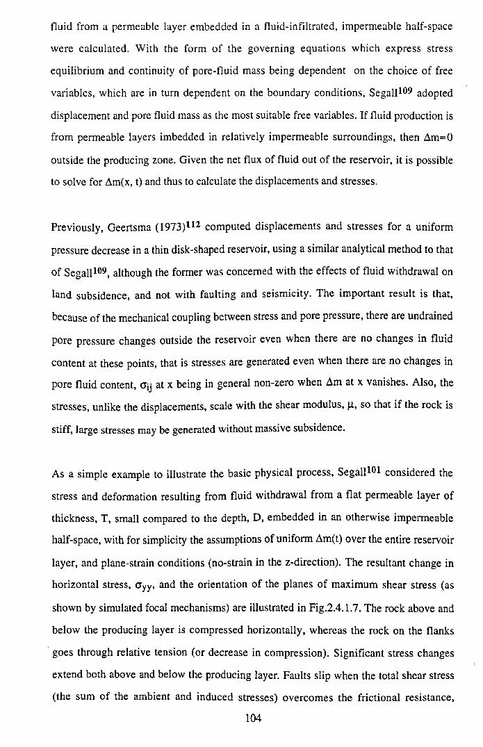
fluid from a permeable layer embedded in a fluid-infiltrated, impermeable half-space

were calculated. With the form of the governing equations which express stress

equilibrium and continuity of pore-fluid mass being dependent on the choice of free

variables, which are in turn dependent on the boundary conditions, Segall109 adopted

displacement and pore fluid mass as the most suitable free variables. If fluid production is

from permeable layers imbedded in relatively impermeable surroundings, then Am=0

outside the producing zone. Given the net flux of fluid out of the reservoir, it is possible

to solve for Am(x, t) and thus to calculate the displacements and stresses.

Previously, Geertsma (1973)112 computed displacements and stresses for a uniform

pressure decrease in a thin disk-shaped reservoir, using a similar analytical method to that

of Segall109, although the former was concerned with the effects o f fluid withdrawal on

land subsidence, and not with faulting and seismicity. The important result is that,

because of the mechanical coupling between stress and pore pressure, there are undrained

pore pressure changes outside the reservoir even when there are no changes in fluid

content at these points, that is stresses are generated even when there are no changes in

pore fluid content, Cij at x being in general non-zero when Am at x vanishes. Also, the

stresses, unlike the displacements, scale with the shear modulus, ji, so that if the rock is

stiff, large stresses may be generated without massive subsidence.

As a simple example to illustrate the basic physical process, Segall101 considered the

stress and deformation resulting from fluid withdrawal from a flat permeable layer of

thickness, T, small compared to the depth, D, embedded in an otherwise impermeable

half-space, with for simplicity the assumptions of uniform Am(t) over the entire reservoir

layer, and plane-strain conditions (no-strain in the z-direction). The resultant change in

horizontal stress, a yy, and the orientation of the planes of maximum shear stress (as

shown by simulated focal mechanisms) are illustrated in Fig.2.4.1.7. The rock above and

below the producing layer is compressed horizontally, whereas the rock on the flanks

goes through relative tension (or decrease in compression). Significant stress changes

extend both above and below the producing layer. Faults slip when the total shear stress

(the sum of the ambient and induced stresses) overcomes the frictional resistance,

104

favoured slip planes therefore depending on the orientation and magnitude of the ambient

stress field (only the component of stress induced by extraction was considered by Segall

as the ambient stress field will vary from site to site). Orientation of the planes of

maximum shear from simulation, predict reverse faulting above and below the producing

zone and normal faulting on its flanks, qualitatively consistent with observations from the

producing field operations described above. Note that the substantial decrease in pressure

within the reservoir inhibits frictional slip within the reservoir rocks themselves. Thus the

stress pattern given in Fig.2.4.1.7 can be understood in a straightforward manner:

(i) fluid extraction causes the reservoir rock to contract

• (ii) contraction in the vertical direction is accommodated by subsidence of the free

surface

(iii) contraction in the horizontal direction is resisted by the surrounding rocks which are

pulled in toward the centre of the reservoir

(iv) strata above and below the reservoir is driven into horizontal compression as a result

of (iii)

(v) rock far away from the reservoir is displaced less than rock immediately above and

below the reservoir, causing the flanking regions to extend

2.4.2 Bedding-parallel Shear

In this section the role of bedding planes as frictional interfaces (planar shear

discontinuities) will be reviewed, and their potential influence as an important

deformation phenomenon in hydrocarbon reservoirs assessed. Particularly in fluvially

deposited arenite rockmasses, initial size, shape and spatial distribution of detrital grains

deposited in an environment controlled by current and gravity, will control the

sedimentary layering o f the material. Grading and composition, in particular the

formation of bedding planes containing clay layers, have first order influence on the

primary anisotropy of the rockmass. Thus a functional fabric formed by vectorial

depositional processes and the resulting preferred dimensional orientation of components

controls the development of primary anisotropy (Moelle & Chappell, 1985113).

' 105

The concept of bedding planes as planes of weakness has been recognised within the

discipline of structural geology for many years. Practically all fault surfaces change their

orientation when they pass through layers of different rock lithology, often showing a

"staircase-like" form in cross-section. The part of a fault which passes at a relatively high

angle through a lithological unit is known as a "ramp" and the section which is sub­

parallel or parallel to the lithology is known as a "flat". The terms ramp and flat are

mostly used in descriptions of low-angle overthrust faults where the hangingwall has

moved upwards over the footwall, but as descriptions they can be applied to differently

inclined sectors of any inclined fault surface. They are generally used irrespective of the

actual geometric orientation of the lithological layering and, for example, a flat can be

steeply inclined where the lithology is steeply inclined. Ramps and flats are connected to

rock "competence" (Ramsay & Huber, 1987114, page 507). In geology, the term

competence is used to describe the differences in rock properties which lead to

mechanical instability, those rocks which flow more easily than their neighbours being

described as the least competent members, those that are stiffer than their neighbours

being termed the most competent rocks. Thus although the term competence is therefore

rather vaguely defined in an exact rheological way, it does give a very useful comparative

description of the components of a layered system, which can be employed in the field to

give some idea of the contrast of the components of a deformed layered system. Ramps

are found in the more competent layers in a succession (massive limestone, conglomerate,

sandstone) whereas flats are found in the incompetent layers (evaporites, shales, marls,

brittle coal horizons).

In rocks which are well-bedded or show a regular planar lamination, the strains set up

during the folding process are often controlled by simple shear parallel to the planar

structure (Ramsay & Huber, pp.445-446). If the simple shear displacement is distributed

continuously throughout the structure then the fold so formed is termed a flexural flow

fold, as shown in Fig.2.4.2.1(a), whereas if the shear is discontinuous the fold is termed a

flexural slip fold as shown in Fig.2.4.2.1(b). Flexural flow folds are generally formed

‘ 106

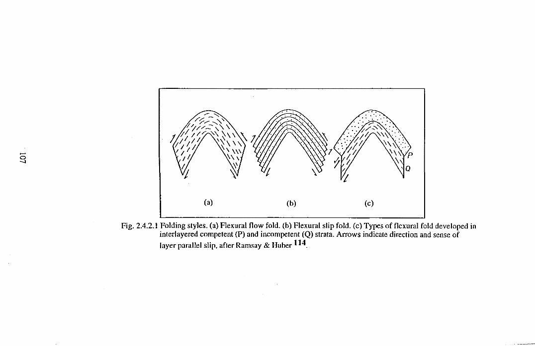
107

Fig. 2.4.2.1 Folding styles, (a) Flexural flow fold, (b) Flexural slip fold, (c) Types of flexural fold developed in interlayered competent (P) and incompetent (Q) strata. Arrows indicate direction and sense oflayer parallel slip, after Ramsay & Huber ^

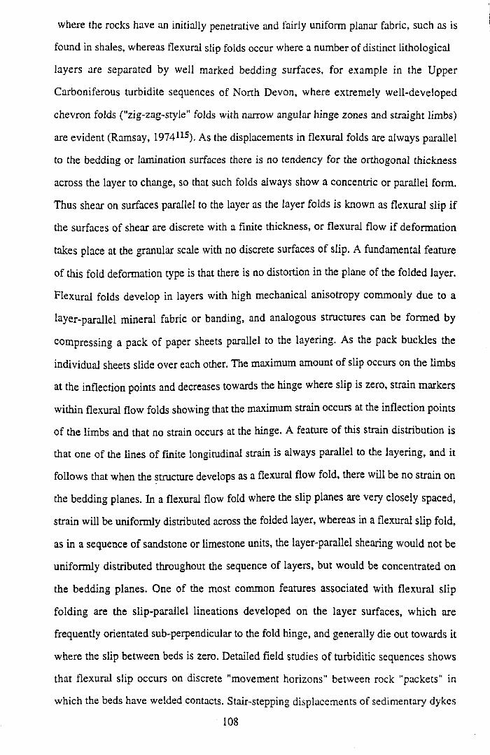
where the rocks have an initially penetrative and fairly uniform planar fabric, such as is

found in shales, whereas flexural slip folds occur where a number of distinct lithological

layers are separated by well marked bedding surfaces, for example in the Upper

Carboniferous turbidite sequences of North Devon, where extremely well-developed

chevron folds ("zig-zag-style" folds with narrow angular hinge zones and straight limbs)

are evident (Ramsay, 1974115). As the displacements in flexural folds are always parallel

to the bedding or lamination surfaces there is no tendency for the orthogonal thickness

across the layer to change, so that such folds always show a concentric or parallel form.

Thus shear on surfaces parallel to the layer as the layer folds is known as flexural slip if

the surfaces of shear are discrete with a finite thickness, or flexural flow if deformation

takes place at the granular scale with no discrete surfaces of slip. A fundamental feature

of this fold deformation type is that there is no distortion in the plane of the folded layer.

Flexural folds develop in layers with high mechanical anisotropy commonly due to a

layer-parallel mineral fabric or banding, and analogous structures can be formed by

compressing a pack of paper sheets parallel to the layering. As the pack buckles the

individual sheets slide over each other. The maximum amount of slip occurs on the limbs

at the inflection points and decreases towards the hinge where slip is zero, strain markers

within flexural flow folds showing that the maximum strain occurs at the inflection points

of the limbs and that no strain occurs at the hinge. A feature of this strain distribution is

that one of the lines of finite longitudinal strain is always parallel to the layering, and it

follows that when the structure develops as a flexural flow fold, there will be no strain on

the bedding planes. In a flexural flow fold where the slip planes are very closely spaced,

strain will be uniformly distributed across the folded layer, whereas in a flexural slip fold,

as in a sequence of sandstone or limestone units, the layer-parallel shearing would not be

uniformly distributed throughout the sequence of layers, but would be concentrated on

the bedding planes. One of the most common features associated with flexural slip

folding are the slip-parallel lineations developed on the layer surfaces, which are

frequently orientated sub-perpendicular to the fold hinge, and generally die out towards it

where the slip between beds is zero. Detailed field studies of turbiditic sequences shows

that flexural slip occurs on discrete "movement horizons" between rock "packets" in

which the beds have welded contacts. Stair-stepping displacements of sedimentary dykes

108

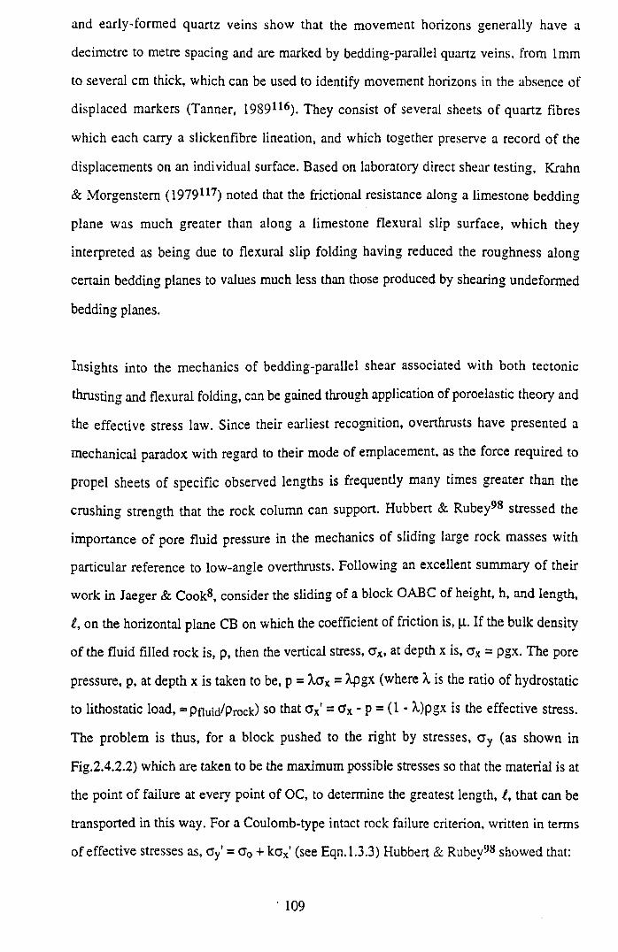
and early-formed quartz veins show that the movement horizons generally have a

decimetre to metre spacing and are marked by bedding-parallel quartz veins, from 1mm

to several cm thick, which can be used to identify movement horizons in the absence of

displaced markers (Tanner, 1989116). They consist of several sheets of quartz fibres

which each carry a slickenfibre lineation, and which together preserve a record of the

displacements on an individual surface. Based on laboratory direct shear testing, Krahn

& Morgenstem (1979117) noted that the frictional resistance along a limestone bedding

plane was much greater than along a limestone flexural slip surface, which they

interpreted as being due to flexural slip folding having reduced the roughness along

certain bedding planes to values much less than those produced by shearing undeformed

bedding planes.

Insights into the mechanics of bedding-parallel shear associated with both tectonic

thrusting and flexural folding, can be gained through application of poroelastic theory and

the effective stress law. Since their earliest recognition, overthrusts have presented a

mechanical paradox with regard to their mode of emplacement, as the force required to

propel sheets of specific observed lengths is frequently many times greater than the

crushing strength that the rock column can support. Hubbert & Rubey98 stressed the

importance of pore fluid pressure in the mechanics of sliding large rock masses with

particular reference to low-angle overthrusts. Following an excellent summary of their

work in Jaeger & Cook8, consider the sliding of a block OABC of height, h, and length,

i, on the horizontal plane CB on which the coefficient of friction is, p.. If the bulk density

of the fluid filled rock is, p, then the vertical stress, Gx, at depth x is, crx = pgx. The pore

pressure, p, at depth x is taken to be, p = Xax = Xpgx (where X is the ratio of hydrostatic

to lithostatic load, ® Pfiuid/Prock) so that a x' = a x - p = (1 - A.)pgx is the effective stress.

The problem is thus, for a block pushed to the right by stresses, Cy (as shown in

Fig.2.4.2.2) which are taken to be the maximum possible stresses so that the material is at

the point of failure at every point of OC, to determine the greatest length, t, that can be

transported in this way. For a Coulomb-type intact rock failure criterion, written in terms

of effective stresses as, c y' = c 0 + k ax' (see Eqn. 1.3.3) Hubbert & Rubey98 showed that:

109

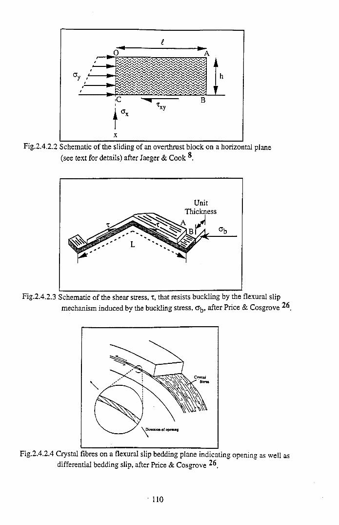
Fig.2.4.2.2 Schematic of the sliding of an overthrust block on a horizontal plane (see text for details) after Jaeger & Cook

Fig.2.4.2.3 Schematic of the shear stress, t, that resists buckling by the flexural slipmechanism induced by the buckling stress, after Price & Cosgrove ^6

Fig.2.4.2.4 Crystal fibres on a flexural slip bedding plane indicating opening as well as differential bedding slip, after Price & Cosgrove ^6

110

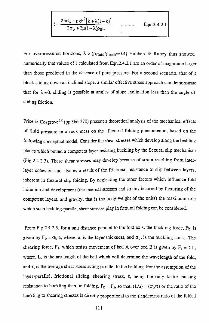
2h g 0 + pgh2[k + X.(l - k)]

2 g 0 + 2 (i(l-X )p g hEqn.2.4.2.1

For overpressured horizons, X > (Pfiuid/p rode5 0-4) Hubbert & Rubey thus showed

numerically that values of i calculated from Eqn.2.4.2.1 are an order of magnitude larger

than those predicted in the absence o f pore pressure. For a second scenario, that of a

block sliding down an inclined slope, a similar effective stress approach can demonstrate

that for A.*0, sliding is possible at angles of slope inclination less than the angle of

sliding friction.

Price & Cosgrove26 (pp.366-370) present a theoretical analysis of the mechanical effects

of fluid pressure in a rock mass on the flexural folding phenomenon, based on the

following conceptual model. Consider the shear stresses which develop along the bedding

planes which bound a competent layer resisting buckling by the flexural slip mechanism

(Fig.2.4.2.3). These shear stresses may develop because of strain resulting from inter­

layer cohesion and also as a result of the frictional resistance to slip between layers,

inherent in flexural slip folding. By neglecting the other factors which influence fold

initiation and development (the internal stresses and strains incurred by flexuring of the

competent layers, and gravity, that is the body-weight o f the units) the maximum role

which such bedding-parallel shear stresses play in flexural folding can be considered.

From Fig.2.4.2.3, for a unit distance parallel to the fold axis, the buckling force, Fb, is

given by Fb = Cb.a, where, a, is the layer thickness, and Ob, is the buckling stress. The

shearing force, Fs, which resists movement of bed A over bed B is given by Fs = x.L,

where, L, is the arc length of the bed which will determine the wavelength of the fold,

and x, is the average shear stress acting parallel to the bedding. For the assumption of the

layer-parallel, frictional sliding, shearing stress, t , being the only factor causing

resistance to buckling then, in folding, Fb = Fs, so that, (L/a) = (C7b/x) or the ratio of the

buckling to shearing stresses is directly proportional to the slenderness ratio of the folded

111

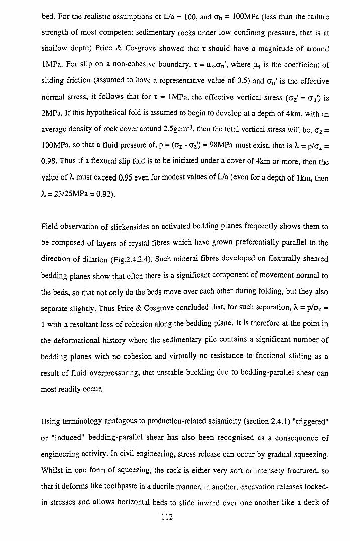
bed. For the realistic assumptions of L/a = 100, and <7b = lOOMPa (less than the failure

strength of most competent sedimentary rocks under low confining pressure, that is at

shallow depth) Price & Cosgrove showed that t should have a magnitude o f around

IMPa. For slip on a non-cohesive boundary, x = where |i s is the coefficient of

sliding friction (assumed to have a representative value of 0.5) and <yn' is the effective

normal stress, it follows that for t = IMPa, the effective vertical stress ( a z' = a n') is

2MPa. If this hypothetical fold is assumed to begin to develop at a depth of 4km, with an

average density of rock cover around 2.5gcm*3, then the total vertical stress will be, az =

lOOMPa, so that a fluid pressure of, p = (ctz - a z') = 98MPa must exist, that is X = p /az =

0.98. Thus if a flexural slip fold is to be initiated under a cover of 4km or more, then the

value of X must exceed 0.95 even for modest values of L/a (even for a depth of 1km, then

X = 23/25MPa = 0.92).

Field observation o f slickensides on activated bedding planes frequently shows them to

be composed of layers of crystal fibres which have grown preferentially parallel to the

direction of dilation (Fig.2.4.2.4). Such mineral fibres developed on flexurally sheared

bedding planes show that often there is a significant component of movement normal to

the beds, so that not only do the beds move over each other during folding, but they also

separate slightly. Thus Price & Cosgrove concluded that, for such separation, X = p/<7z =

1 with a resultant loss of cohesion along the bedding plane. It is therefore at the point in

the deformational history where the sedimentary pile contains a significant number of

bedding planes with no cohesion and virtually no resistance to frictional sliding as a

result o f fluid overpressuring, that unstable buckling due to bedding-parallel shear can

most readily occur.

Using terminology analogous to production-related seismicity (section 2.4.1) "triggered"

or "induced" bedding-parallel shear has also been recognised as a consequence of

engineering activity. In civil engineering, stress release can occur by gradual squeezing.

Whilst in one form of squeezing, the rock is either very soft or intensely fractured, so

that it deforms like toothpaste in a ductile manner, in another, excavation releases locked-

in stresses and allows horizontal beds to slide inward over one another like a deck of

112

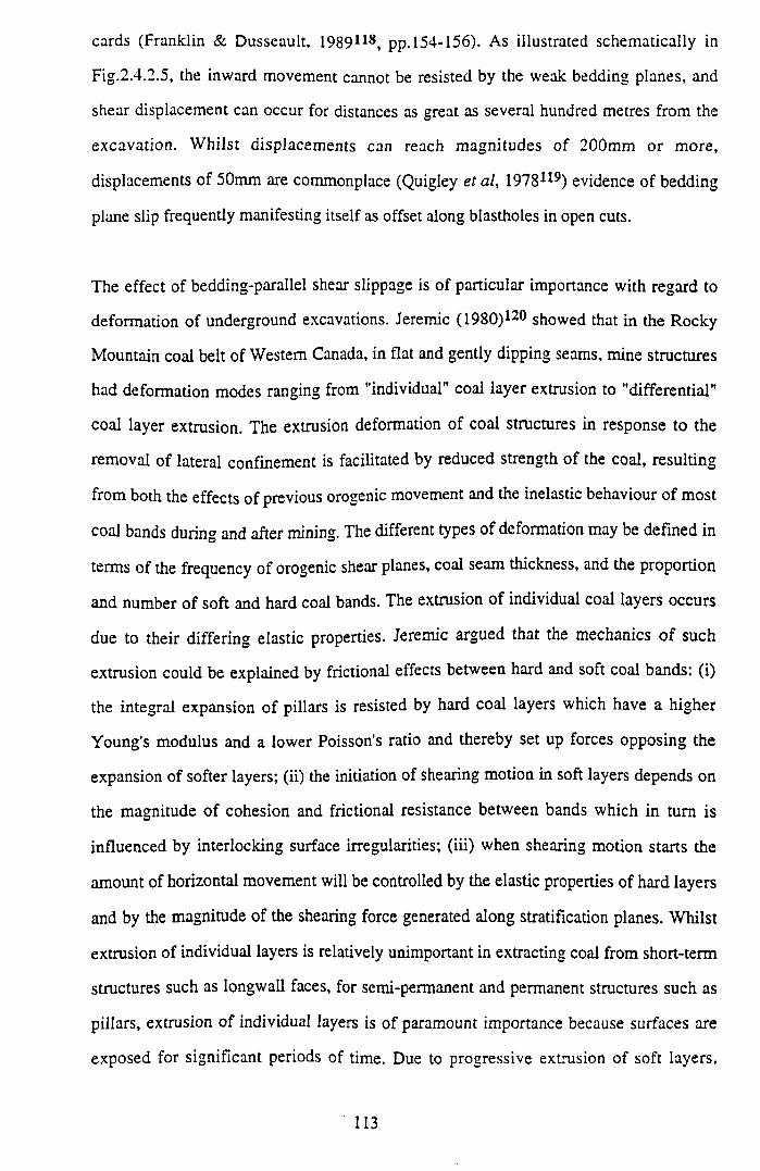
cards (Franklin & Dusseault, 1989118, pp. 154-156). As illustrated schematically in

Fig.2.4.2.5, the inward movement cannot be resisted by the weak bedding planes, and

shear displacement can occur for distances as great as several hundred metres from the

excavation. W hilst displacements can reach m agnitudes of 200mm or more,

displacements of 50mm are commonplace (Quigley etal, 1978119) evidence of bedding

plane slip frequently manifesting itself as offset along blastholes in open cuts.

The effect of bedding-parallel shear slippage is of particular importance with regard to

deformadon of underground excavations. Jeremic ( 1980)120 showed that in the Rocky

Mountain coal belt of Western Canada, in flat and gently dipping seams, mine structures

had deformation modes ranging from "individual" coal layer extrusion to "differential"

coal layer extrusion. The extrusion deformation of coal structures in response to the

removal of lateral confinement is facilitated by reduced strength of the coal, resulting

from both the effects of previous orogenic movement and the inelasuc behaviour of most

coal bands during and after mining. The different types of deformation may be defined in

terms of the frequency of orogenic shear planes, coal seam thickness, and the proportion

and number o f soft and hard coal bands. The extrusion of individual coal layers occurs

due to their differing elastic properties. Jeremic argued that the mechanics o f such

extrusion could be explained by frictional effects between hard and soft coal bands: (i)

the integral expansion of pillars is resisted by hard coal layers which have a higher

Young's modulus and a lower Poisson's ratio and thereby set up forces opposing the

expansion of softer layers; (ii) the initiation of shearing motion in soft layers depends on

the magnitude of cohesion and frictional resistance between bands which in turn is

influenced by interlocking surface irregularities; (iii) when shearing motion starts the

amount of horizontal movement will be controlled by the elastic properties of hard layers

and by the magnitude of the shearing force generated along stratification planes. Whilst

extrusion of individual layers is relatively unimportant in extracting coal from short-term

structures such as longwall faces, for semi-permanent and permanent structures such as

pillars, extrusion o f individual layers is of paramount importance because surfaces are

exposed for significant periods of time. Due to progressive extrusion of soft layers,

113

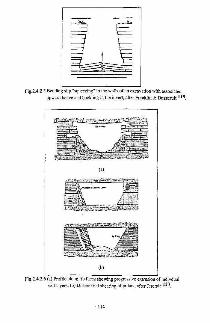
Fig.2.4.2.5 Bedding slip "squeezing” in the walls of an excavation with associated upward heave and buckling in the invert, after Franklin & Dusseault

Fig.2.4.2.6 (a) Profile along rib faces showing progressive extrusion of indivdual soft layers, (b) Differential shearing of pillars, after Jeremic 1-° .

114

unsupported fragments of hard coal layers in the outer zone of pillars have a tendency to

break and fall into roadways as shown in Fig.2.4.2.6(a). The mechanics of extrusion

deformation by differential shearing, which was particularly well-exhibited in thick coal

seams, is also governed by frictional effects between stratification planes, as shown in

Fig.2.4.2.6(b). Here the differential deformation results from differential shear resistance

at the top and bottom of the seam, where, for example, there may be a high magnitude of

constraint between the top coal slice and a massive sandstone of high elastic modulus and

a moderate amount of restraint between the bottom coal slice and the inelastic floor

stratum, or vice versa.

To quantify shearing deformation of mine structures, shear strength characteristics of

different petrographic coal units and of mudstone partings were tested under direct shear

laboratory conditions using constant normal load control. For all three coal types tested

the peak friction angle of coal bedding planes was constant at about 34°, whereas the

apparent cohesion varied appreciably from 0.35-1.2MPa, hard coal and brittle coal having

a greater cohesion than fibrous coal. As the great majority of sheared bedding planes are

vitrinite (brittle) bands, however, cohesion is of lesser importance in determining mine

stability because it resists only the initial shearing stress, the main strength component

being residual frictional resistance. The residual friction angle was found to be 27° with

zero cohesion. Direct shear testing of carbonaceous and shaley parting planes showed

these stratification contacts to have only residual strength, with an average friction angle

of 28° and zero cohesion, similar to the residual shear behaviour of coal bedding planes.

In conclusion, Jeremic noted that mine stability is greatly controlled by the shearing

characteristics between individual bands with differing petrographic characteristics within

coal seams, shear displacement along stratification planes being mobilised by the

redistribution of excess overburden pressure in the mine structure, as well as by frictional

effects between individual layers of different mechanical properties. Thus Jeremic noted

that the "classical" approach for excavation design in coal seams using the uniaxial

compressive strength of coal is of lesser significance in the Rocky Mountain belt as the

shear strength of coal seams is lower than in other coal regions of the world, with

115

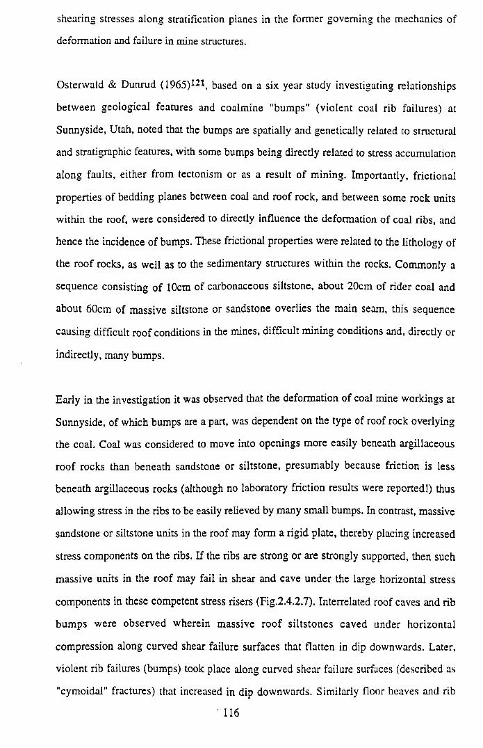
shearing stresses along stratification planes in the former governing the mechanics of

deformation and failure in mine structures.

Osterwald & Dunrud (1965)121, based on a six year study investigating relationships

between geological features and coalmine "bumps" (violent coal rib failures) at

Sunnyside, Utah, noted that the bumps are spatially and genetically related to structural

and stratigraphic features, with some bumps being directly related to stress accumulation

along faults, either from tectonism or as a result of mining. Importantly, frictional

properties of bedding planes between coal and roof rock, and between some rock units

within the roof, were considered to directly influence the deformation of coal ribs, and

hence the incidence of bumps. These frictional properties were related to the lithology of

the roof rocks, as well as to the sedimentary structures within the rocks. Commonly a

sequence consisting of 10cm of carbonaceous siltstone, about 20cm of rider coal and

about 60cm of massive siltstone or sandstone overlies the main seam, this sequence

causing difficult roof conditions in the mines, difficult mining conditions and, directly or

indirectly, many bumps.

Early in the investigation it was observed that the deformation of coal mine workings at

Sunnyside, of which bumps are a part, was dependent on the type of roof rock overlying

the coal. Coal was considered to move into openings more easily beneath argillaceous

roof rocks than beneath sandstone or siltstone, presumably because friction is less

beneath argillaceous rocks (although no laboratory friction results were reported!) thus

allowing stress in the ribs to be easily relieved by many small bumps. In contrast, massive

sandstone or siltstone units in the roof may form a rigid plate, thereby placing increased

stress components on the ribs. If the ribs are strong or are strongly supported, then such

massive units in the roof may fail in shear and cave under the large horizontal stress

components in these competent stress risers (Fig.2.4.2.7). Interrelated roof caves and rib

bumps were observed wherein massive roof siltstones caved under horizontal

compression along curved shear failure surfaces that flatten in dip downwards. Later,

violent rib failures (bumps) took place along curved shear failure surfaces (described as

"cymoidal" fractures) that increased in dip downwards. Similarly floor heaves and rib

116

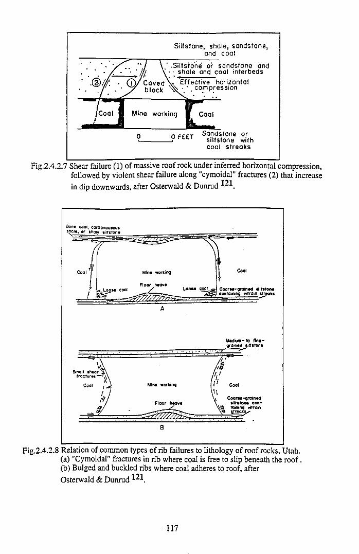
Silt stone, shale, sandstone, and coal

Fig.2.4.2.7 Shear failure (1) of massive roof rock under inferred horizontal compression, followed by violent shear failure along "cymoidal" fractures (2) that increasein dip downwards, after Osterwald & Dunrud 121.

Fig.2.4.2.8 Relation of common types of rib failures to lithology of roof rocks, Utah.(a) "Cymoidal" fractures in rib where coal is free to slip beneath the ro o f.(b) Bulged and buckled ribs where coal adheres to roof, afterOsterwald & Dunrud ^ .

117

bumps that were probably interrelated were observed. Ribs in the Sunnyside mines

commonly fail in one of two ways. Where coal is free to slip beneath the roof, "cymoidal"

shear fractures form within the ribs, and where coal adheres to the roof, the ribs bulge and

buckle (see Fig.2.4.2.8). Most bumps result from failure along "cymoidal' fractures, but

loose coal is thrown down from some bulged ribs during bumps. Commonly one rib will

fail along "cymoidal" shear fractures whereas the opposite rib will fail by bulging and

buckling, implying that coal is free to slip beneath the roof in one direction, but not in the

other. Osterwald & Dunrud considered this probably to be the result of original

sedimentary features in the bedding surfaces, such as ripple marks, channel Fills, load

casts, crossbeds and slump structures, which impart pronounced but variable differences

to the frictional properties of the slip surfaces in different directions.

Smart (1991)122 contends that deformation, not just of coal sequences, but o f all tabular

deposits, is controlled by "dominant parting planes" (DPP's) particularly with regard to

the release of strain energy around an excavation. A DPP is here defined as, "a laterally

extensive but thin natural feature parallel to bedding which allows both relative normal

motion (separation) and importantly parallel motion (shear) between adjacent strata." The

argument is that, even at moderate depth, DPP's controlled by sedimentology will be

activated in shear ahead of excavations such as longwall coalfaces, due to the release of

horizontal stresses in the strata. This shearing action creates striations in a layer of

frictional wear debris on the partings, which tend to point towards the approaching

excavation and the associated release of horizontal stress. Importantly, Smart used finite

element modelling to study the process of strata deformation in the vicinity of a gateroad

and longwall coalface, finding a significant reduction in strain energy when shear was

permitted along DPP's, compared with an equivalent model in which the same bedding

planes were pinned. Thus DPP's were considered to represent an energetically favourable

strata deformation mechanism. Considering the models to be lm thick sections, a 4.8MJ

reduction in strain energy was associated with the treatment of DPP's as frictional

interfaces.

118

Whilst the above summary highlights the importance of bedding-parallel shear as a

natural mechanism for the accommodation of tectonic strain, particularly under

conditions of high fluid overpressure, and emphasises the role of bedding-parallel shear

as a means of stress release associated with civil and mining engineering excavations, the

main point in question is whether or not it occurs in the hydrocarbon reservoir

environment in association with stress perturbations resulting from production. The best

evidence for such slip on bedding planes lies in the generation of shallow focus

earthquakes at Wilmington oil field in Long Beach, California, associated with fluid

extraction, as discussed in section 2.4.1. Here six earthquakes (M2.4 to 3.3) were

generated by bedding plane shear at depths of 470 to 520m (Kovach102). The significance

of this phenomenon with regard to its potential effect on production operations is readily

assessed from consideration of the results at Wilmington, where tens to hundreds of wells

were sheared off over several square kilometres. As far as the author is aware, no

incidences of induced earthquakes due to bedding-parallel slip resulting from fluid

injection operations have been reported in the literature, which is perhaps surprising

considering the role of fluid overpressure with regard to theories of tectonic thrusting and

flexural slip folding.

Im portant corroborative evidence for bedding-parallel slip resulting from fluid

withdrawal is provided by unpublished finite element modelling of a producing wellbore

conducted within the Department of Petroleum Engineering, Heriot-Watt University, by

Mr.P.W.H.Olden (pers. comm.). The model represented an idealised producing oil

reservoir horizon, and was constructed using the ANSYS program, from 130 solid

elements and 88 frictional interface elements in an axisymmetric formulation, the

wellbore taken to be along the y-(vertical) axis. The model represented a 50m thick

central producing horizon, with respectively, 50m and 30m of stratified rock mass above

and below it, each containing frictionless bedding planes at regular lOm-spaced intervals.

The model was assumed to be composed of a single rock type with elastic deformation

and failure strength properties indicative of a moderately weak sandstone. An important

feature of this model was the coefficient of thermal expansion used for the material.

' 119

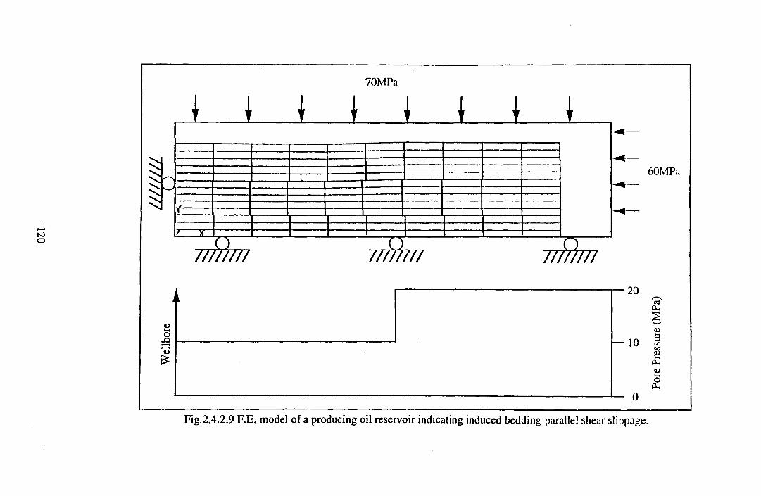
120

70MPa

60MPa

Cu,

aDcn<Da,<uocu

Fig.2.4.2.9 F.E. model o f a producing oil reservoir indicating induced bedding-parallel shear slippage.

which enabled the effect of pore pressure to be simulated through analogy with thermal

strain. By using a coefficient of thermal expansion, a , expressed by:

(1 — 2 v )(X = ------------ 1 - 7 4 7 1

E l Ks J

where E is Young's modulus, v is Poisson's ratio and Kb and Ks are the bulk moduli of

the rock and the rock matrix respectively. Assuming (1-Kb/Ks) = 1, pore pressures are

simply input by using element temperatures (Warren & Smith, 1985123). For remote

stresses and boundary conditions as shown in Fig.2.4.2.9, a transient of lOMPa in the

initial ubiquitous pore pressure of 20MPa throughout the stratigraphy was modelled

(shown in detail in Fig.2.4.2.9) to simulate fluid withdrawal. The finite element mesh of

Fig-2.4.2.9 represents a displacement plot, however relative displacements have been

magnified for the purposes of clarity. The immediately noticeable point is that interlayer

slip has occurred above and below the producing horizon to accommodate strain

associated with fluid withdrawal, with a maximum of about 0.1m displacement occurring

near the centre of the model. A complementary plot of horizontal stress distribution in the

sequence of beds overlying the producing horizon shows that the net effect is for tensile

stresses to be induced in the convex side of the sequence, and compressive stresses on the

concave side. Relative subsidence from wellbore to outer edge of the model, associated

with fluid withdrawal, is of the order of 45mm.

121

3. DIRECT SHEAR EXPERIM ENTATION: RIG DESIGN AND RESULTS

3.1 INTRODUCTION

Current rock mechanics “philosophy” regards the rockmass as a composite material

consisting of two principal components: interbedded lithologies (intact rock types)

characterised by porosity, mineralogy, grain texture, degree of microcracking etc. and

discontinuities characterised by population statistics (size distribution and 3-D

orientation) mode of genesis, roughness, infilling etc. The global mechanical behaviour

of a typical hydrocarbon reservoir rockmass (stratified, transected by discontinuities) is

governed by its deformability and strength characteristics. Natau (1990)124 suggests that

these characteristics in the simplest sense can be described by an elasto-plastic

constitutive relation determined by a global Young’s modulus, Eg, a global Poissons

ratio, vg, a global friction angle, <|>g, and a global cohesion, cg, (Fig.3.1.1). These global

characteristics in turn are determined by the behaviour and interaction of the rockmass’s

individual components. The stress-strain behaviour of the intact rock is determined by

the Young’s modulus, Ej, and Poissons ratio, Vi, of each lithology, whilst strength criteria

can be expressed using an internal friction angle, 0 ¡, and a cohesion, Cj. Standard uniaxial

and triaxial tests for estimating these intact rock parameters are conducted within

compression rigs. The mechanical properties of the discontinuities are also dependent on

the properties of the intact host rock itself. Constitutive laws for discontinuities consist of

descriptions of the discontinuity deformability (normal and shear stiffnesses, kn and ks)

and strength criteria (discontinuity friction angle, 0d, and cohesion, Cd). These parameters

are estimated experimentally using a direct shear rig. Direct shear testing should

therefore be perceived as being of equal importance with the more conventional uniaxial

and triaxial compression tests, in determining rockmass deformability and strength

parameters.

3.2 D IRECT SHEAR RIG DESIGN

The Heriot-Watt servo-hydraulic direct shear rig was conceived as an essential addition

to the existing rock mechanics experimental facility (centred around a 100T stiff

compression machine as described in Chapter 4) to enable the testing o f rock

122

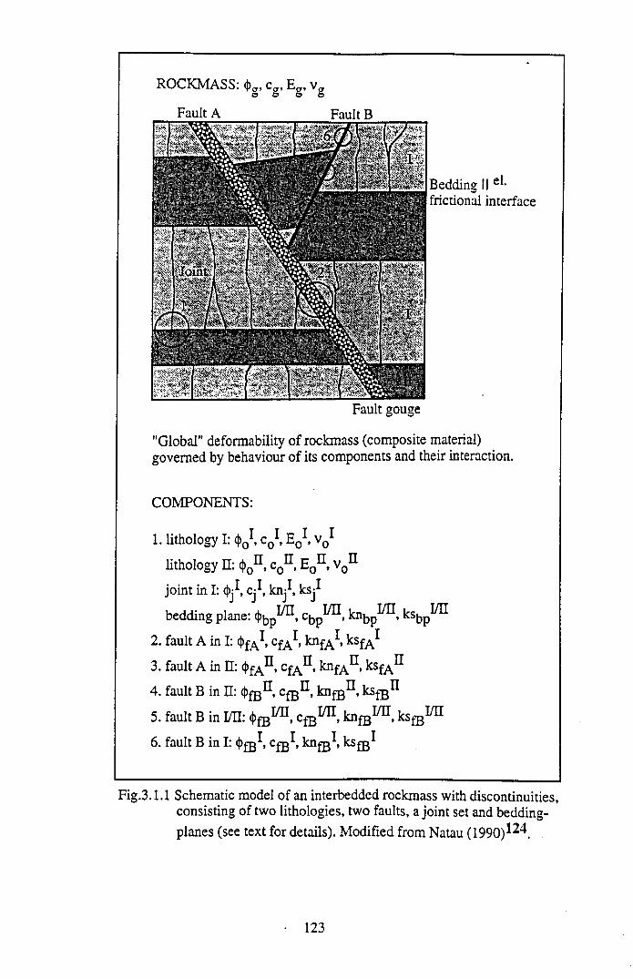
ROCKMASS: <{>„, C{r, Eg, v g

Fault A Fault B

....... ^ . ^ Bedding II e -frictional interface

> Tt-t *v?-A*,v' >3

Fault gouge

"Global" deformability of rockmass (composite material) governed by behaviour of its components and their interaction.

COMPONENTS:

1. lithology I: c j , E0l , vQl

lithology II: <{>0n , c0n , E0n , v0n

joint in I: <j)j Cj*, knj*, ksj^

bedding plane: ^ b p ^ ’ ^ b p 1 ’ ksbpI/n

2. fault A in I: (})fA^ Cf^> k n ^ » ksfA^

3. fault A in II: cfA^* ^ f A ^ ’ ksfA ^

4. fault B in II: Cfg11, ^ fB 11’ ^ f B 11

5. fault B in I/H: fa ™ 1, c® 111, kn® 1711. ksffi1711

6. fault B in I: cfB^» kn®*» ksfgl

Fig.3.1.1 Schematic model of an interbedded rockmass with discontinuities, consisting of two lithologies, two faults, a joint set and bedding-planes (see text for details). Modified from Natau (1990)124

123

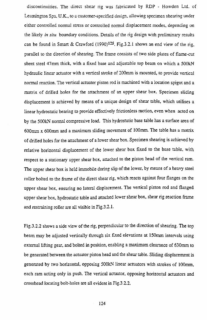
discontinuities. The direct shear rig was fabricated by RDP - Howden Ltd. of

Leamington Spa, U.K., to a customer-specified design, allowing specimen shearing under

either controlled normal stress or controlled normal displacement modes, depending on

the likely in situ boundary conditions. Details of the rig design with preliminary results

can be found in Smart & Crawford (1990)125. Fig.3.2.1 shows an end view of the rig,

parallel to the direction of shearing. The frame consists of two side plates of flame-cut

sheet steel 47mm thick, with a fixed base and adjustable top beam on which a 500kN

hydraulic linear actuator with a vertical stroke of 200mm is mounted, to provide vertical

normal reaction. The vertical actuator piston rod is machined with a location spigot and a

matrix of drilled holes for the attachment of an upper shear box. Specimen sliding

displacement is achieved by means of a unique design of shear table, which utilises a

linear hydrostatic bearing to provide effectively frictionless motion, even when acted on

by the 500kN normal compressive load. This hydrostatic base table has a surface area of

600mm x 600mm and a maximum sliding movement of 100mm. The table has a matrix

of drilled holes for the attachment of a lower shear box. Specimen shearing is achieved by

relative horizontal displacement of the lower shear box fixed to the base table, with

respect to a stationary upper shear box, attached to the piston head of the vertical ram.

The upper shear box is held immobile during slip of the lower, by means of a heavy steel

roller bolted to the frame of the direct shear rig, which reacts against four flanges on the

upper shear box, ensuring no lateral displacement. The vertical piston rod and flanged

upper shear box, hydrostatic table and attached lower shear box, shear rig reaction frame

and restraining roller are all visible in Fig.3.2.1.

Fig.3.2.2 shows a side view of the rig, perpendicular to the direction of shearing. The top

beam may be adjusted vertically through six fixed elevations at 150mm intervals using

external lifting gear, and bolted in position, enabling a maximum clearance of 630mm to

be generated between the actuator piston head and the shear table. Sliding displacement is

generated by two horizontal, opposing 500kN linear actuators with strokes of 100mm,

each ram acting only in push. The vertical actuator, opposing horizontal actuators and

crosshead locating bolt-holes are all evident in Fig.3.2.2.

124

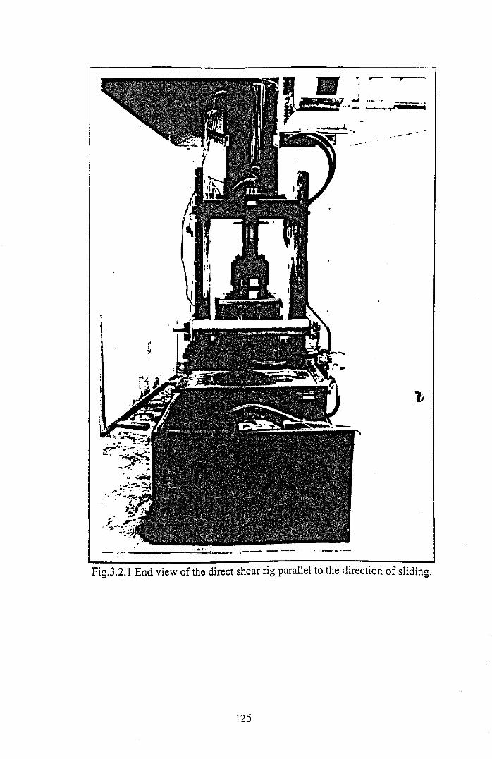
125

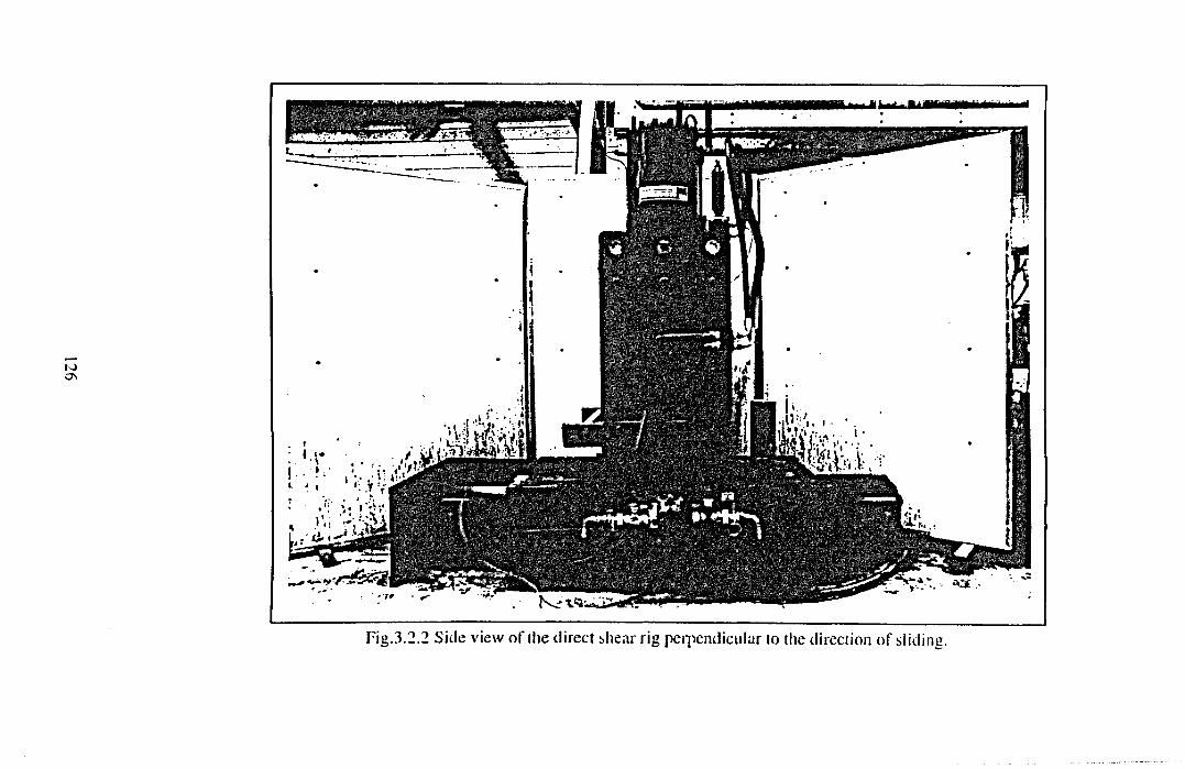
IOON

Fig.3.2.2 Side view of the direct shear rig perpendicular to the direction of sliding.

Fig.3.2.3 shows a scaled schematic of the direct shear rig (both front and back elevations

perpendicular to the direction of shearing) detailing the hydraulic supply and control

systems. A constant pressure oil supply for the vertical and horizontal actuator servo

systems is provided by a mobile hydraulic power pack with a maximum system pressure

of 30MPa (4300psi). This power pack also supplies the 100T compression rig and

pressure intensifier for triaxial testing. The shear table linear hydrostatic bearing is fed

from a separate mobile hydraulic power pack which supplies a maximum system pressure

of up to 20MPa (3000psi), and scavenges the spent oil. The bearing action is created by

feeding hydraulic oil through four orifices on the underside of the shear table. The 20MPa

system pressure is dissipated in a 0.05 mm gap between the rims of the orifices and a

lower bearing plate. The linear actuator providing vertical thrust is an unequal area,

double acting unit capable of producing greater compressive than tensile forces. It is

suitable for operation under closed loop control with displacement or pressure as the

controlling parameter. A servo-valve manifold block, high pressure accumulator,

displacement and pressure transducers are fitted as standard. An internal LVDT provides

measurement of piston travel for normal displacement control, whilst a pressure

transducer in the hydraulic feed line enables the actuator to be operated under the

alternative condition of normal load control. The vertical ram is controlled from an RDP-

Howden System 2000 Command Module, a control console also used to direct the

compression rig and confining pressure facilities. This unit theoretically allows any

parameter conditioned to a 0 - 10V scale to control the vertical actuator, for example a

load cell could provide an alternative means of normal load measurement (shown dotted

in Fig.3.2.3) although for the tests described here, only closed loop pressure transducer

control was utilised. Although both axial load and confining pressure can be controlled

simultaneously using the System 2000, triaxial and direct shear tests cannot be performed

at the same time, so that servo-valve and transducer connections to the control console

have to be swapped around depending on which test is to be conducted. The pair of single

acting (push-only) horizontal actuators mounted either side of the hydrostatic shear table

are controlled separately from the vertical ram. LVDT’s allow measurement of horizontal

displacement, whilst pressure transducers in the hydraulic feed-lines enable measurement

of shear loads. A bench console provides control of the horizontal actuators. This

127

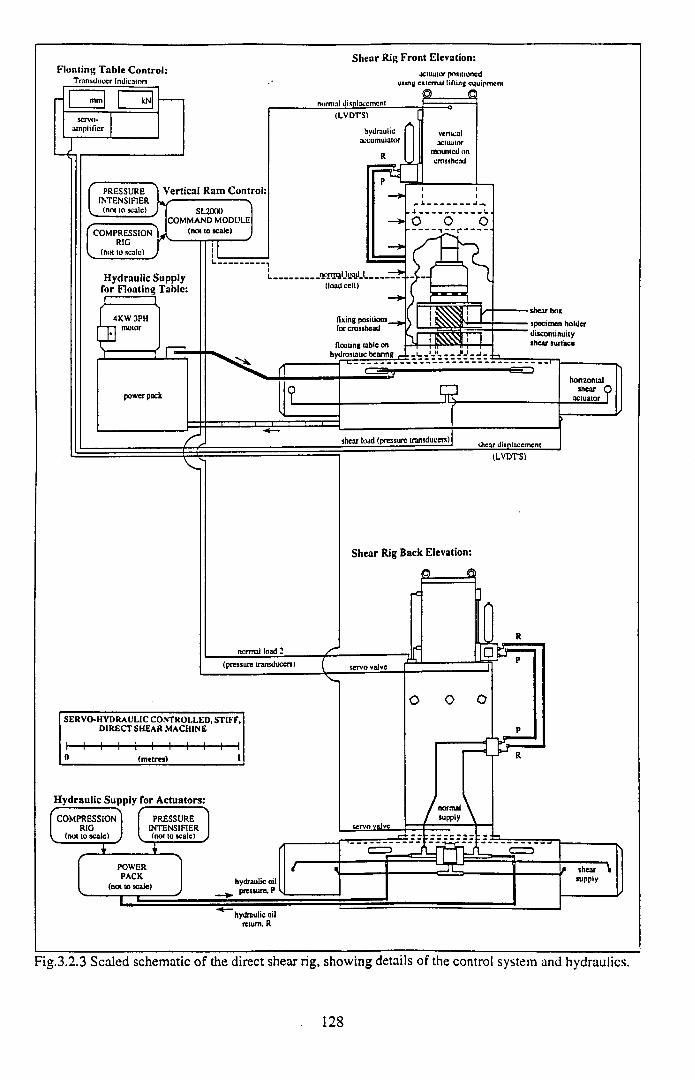
Floating Table Control:Transducer Indicators

1 m J 1 Mservo-

amplifier

Shear Rig Front Elevation:actuator positioned

using external lifting equipment

____ Q

PRESSURE INTENSIFIER

(not to scale)

Vertical Ram Control:

COMPRESSIONRIG

(not to scale)

V“--------------- \SL2000

COMMAND MODULE . (not to scale)A—

Hydraulic Supply for Floating Table:

4KW 3PH motor

power pock

normal displacement(LVDTS)

I---------- -.no^rpa!JoqjlJ. . . . _y . .

(load cell)

fixing positions . for crosshead

floating table on hydrostatic bearing ,

vertical actuator

mounted on cmsshcad

M-I__JU . j .

•shear box

- specimen holder * discontinuity

shear surface

? JS

x

shear load (pressure transducers) shear displacement

horizontalshear

actuator î

normal load 2

(LVDTS)

Shear Rig Back Elevation:

0_____£

(pressure transducers) servo valve

SERVO-HYDRAULIC CONTROLLED, STIFF. DIRECT SHEAR MACHINE

1----1---- 1---- 1----1----1----1---- 1----1---- !----1(metres)

Hydraulic Supply for Actuators:/ -----------------------\

COMPRESSION PRESSURERIG INTENSIFIER

k (not to scale) L (nono scale) J

POWER PACK

(not to scale) hydraulic oil pressure. P

Mo o o

hydraulic oil return. R

shear ■ supply

'ig.3.2.3 Scaled schematic o f the direct shear rig, showing details of the control system and hydraulics.

128

comprises a servo amplifier to supply the drive current for the servo-valve, and a dual

amplifier/monitor unit with transducer indicators giving digital displays in mm and kN

respectively. Hardcopy data from tests performed under constant normal displacement

conditions is provided in the form of continuous line traces of normal load, shear load

and normal displacement against shear displacement, recorded on a multi-channel,

moving-paper chart-recorder.

3.3 TEST SPECIMENS AND EXPERIMENTAL METHODOLOGY

To facilitate initial appraisal of direct shear rig performance, the frictional strengths of a

dozen cylindrical test specimens sourced from a wide range of sedimentary rock types

were measured, all under constant normal displacement conditions. The main variable in

the experimental programme was therefore lithology. Cylindrical test specimens were

produced by coring large (typically 100kg) blocks obtained from quarrying and open cast

mining operations. The diameter of the core samples (around 4.5” or 118mm) is directly

equivalent to a standard size of reservoir whole core routinely taken when retrieving core

from exploration and production wells. Brief lithological descriptions of the twelve

specimens tested in direct shear are given below: three were red medium-grained aeolian

sandstones, specifically quartz arenites consisting of predominantly quartz grains and

some potassium feldspar, with significant haematite cement coating the grains (specimens

#3, #5 and #6); two were dark grey, highly fissile mudrocks (specimens #8 and #9)

specimen #8 possessing some minor silty laminae, specimen #9 appearing homogeneous

and predominantly composed of clay-grade material; three were planar laminated, highly

heterolithic siltstones (specimens #11, #12 and #14) consisting of dark-grey/black

carbonaceous, laminated siltstone with profuse plant debris, containing variable numbers

of up to cm-thick bands of white fine-grained quartz arenite sandstone; four were grey,

highly heterolithic, inter-banded sandstones and siltstones (specimens SI, S2, S3 and S4)

consisting of thickly laminated fine sandstone and siltstone layers with varying clay

contents, showing signs of significant soft sediment deformation resulting in undulose

and non-planar bedding. Individual core specimen identification numbers are given in the

brackets following the above lithological descriptions.

129

From the above, it is evident that the direct shear specimens fall broadly into four distinct

rock types: the red medium sandstones #3, #5 and #6; the dark-grey fissile mudrocks #8

and #9; the black carbonaceous siltstones #11, #12 and #14; the grey heterolithic

siltstones S I, S2, S3 and S4. Whilst the red sandstone specimens appear broadly

homogeneous on the core specimen scale, with only faint traces of a planar cross-

lamination so that between-sample variation is low, specimens from the remaining three

lithological groups show higher degrees of sedimentological heterogeneity, and thus

higher between-sample variation for each rock type. Both mudrock specimens show

strong fissility on shaley partings perpendicular to their long axes, however between-

sample variation is moderate and due primarily to the existence of silty laminae in #8 not

seen in #9, the latter being almost 100% claystone. The black carbonaceous siltstones

also show moderate discrepancies in between-sample sedimentology due to bands of

variable thickness, white, fine-grained sandstone being present with different frequency

in each specimen. However, greatest between-sample lithological variability is shown by

the grey inter-banded sandstones/siltstones, where their heterolithic nature combined with

varying degrees of chaotic bed disruption due to soft sediment deformation, has resulted

in widely different quartz, feldspar, clay and muscovite percentage mineral contents. X-

ray diffraction analyses of >500micron-sized fault gouge fractions, obtained by sieving

shear debris sampled from the sliding surfaces of each of the post-test direct shear

specimens, provide approximate quantification of initial specimen mineralogy’s. Such

XRD-derived percentage mineral contents from specimens #3, #5, #8, #9, #12, #14, S I,

S2, S3 and S4 are presented in Chapter 6.

To mount a cylindrical specimen in the direct shear rig, upper and lower core holders

(steel hollow cylindrical sheaths bolted to the rock core) are fitted to the specimen so that

a 10mm gap is left between them to accommodate the shear plane. The specimen with its

core holders is then positioned in the lower shear box, and the upper shear box carefully

lowered over it until flush with the specimen top surface. The core holders are then bolted

securely into the shear boxes. Whilst the core holders used are machined specifically to

fit specimens 118mm (4.5”) in diameter, the shear boxes could accommodate core up to

about 200mm (8”) with suitably sized core holders. Due to the depth of the shear boxes,

130

core samples must be some 300mm in length, necessitating the capping of some

undersized specimens with quick-setting, high-strength concrete. To aid in the capping

process, split moulds were constructed.

An interesting indirect consequence of the difference in lithology shown by the test

specimens was reflected in the nature of the discontinuity introduced into each prior to

shearing. Each specimen was initially “notched” using a hammer and chisel at the desired

location for the intended shear plane, secured in the shear boxes as described above,

leaving a 10mm gap containing the notch between the upper and lower shear boxes, and

then “popped” in tension using the normal load actuator to pull apart the specimen halves.

The discontinuity introduced into the red sandstones by this means proved to be a rough

planar tensile fracture that had propagated from the circumferential notch with no

lithological control. In contrast, discontinuities induced in the fissile mudstone

specimens corresponded to smooth, fissile shaley partings. The carbonaceous siltstones

also produced discontinuities within the notched region controlled by sedimentary

lamination, being largely carbonaceous and micaceous bedding parallel partings. The

grey heterolithic sandstones/siltstones tended to produce concavo-convex tensile

fractures, partially associated with clay-rich laminae within the vicinity of the notched

region, but also cross-cutting sandier bands. The chaotic nature of the bedding due to soft

sediment deformation meant that the discontinuities were more undulose than those in the

other lithologies, with between-sample variation in discontinuity surface roughness being

much greater in specimens SI, S2, S3 and S4. Specimen surface roughness appeared to

be fairly constant within the red sandstone, fissile mudstone and carbonaceous siltstone

rock types.

To conduct a direct shear test, following the creation of a discontinuity in tension as

described above, the specimen halves were re-mated with the pre-shear discontinuity

protruding, respectively, some 5mm below and above the upper and lower core holders.

A normal stress of around l.OMPa (minimum 0.7MPa for #9, maximum 2.7MPa for #3)

was then applied across the discontinuity, prior to shearing the upper and lower specimen

halves relative to each other on this plane. Horizontal displacement of the lower specimen

131

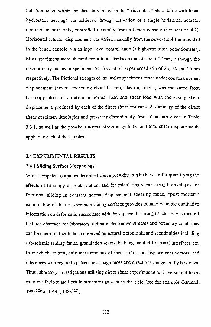
half (contained within the shear box bolted to the “frictionless” shear table with linear

hydrostatic bearing) was achieved through activation of a single horizontal actuator

operated in push only, controlled manually from a bench console (see section 4.2).

Horizontal actuator displacement was varied manually from the servo-amplifier mounted

in the bench console, via an input level control knob (a high-resolution potentiometer).

Most specimens were sheared for a total displacement of about 20mm, although the

discontinuity planes in specimens SI, S2 and S3 experienced slip of 23, 24 and 25mm

respectively. The frictional strength of the twelve specimens tested under constant normal

displacement (never exceeding about 0.1mm) shearing mode, was measured from

hardcopy plots of variation in normal load and shear load with increasing shear

displacement, produced by each of the direct shear test runs. A summary of the direct

shear specimen lithologies and pre-shear discontinuity descriptions are given in Table

3.3.1, as well as the pre-shear normal stress magnitudes and total shear displacements

applied to each of the samples.

3.4 EXPERIMENTAL RESULTS

3.4.1 Sliding Surface Morphology

W hilst graphical output as described above provides invaluable data for quantifying the

effects of lithology on rock friction, and for calculating shear strength envelopes for

frictional sliding in constant normal displacement shearing mode, “post mortem”

examination of the test specimen sliding surfaces provides equally valuable qualitative

information on deformation associated with the slip event. Through such study, structural

features observed for laboratory sliding under known stresses and boundary conditions

can be contrasted with those observed on natural tectonic shear discontinuities including

sub-seismic sealing faults, granulation seams, bedding-parallel frictional interfaces etc.

from which, at best, only measurements of shear strain and displacement vectors, and

inferences with regard to palaeostress magnitudes and directions can generally be drawn.

Thus laboratory investigations utilising direct shear experimentation have sought to re ­

examine fault-related brittle structures as seen in the field (see for example Gamond,

1983126 and Petitf 1988127 ).

132

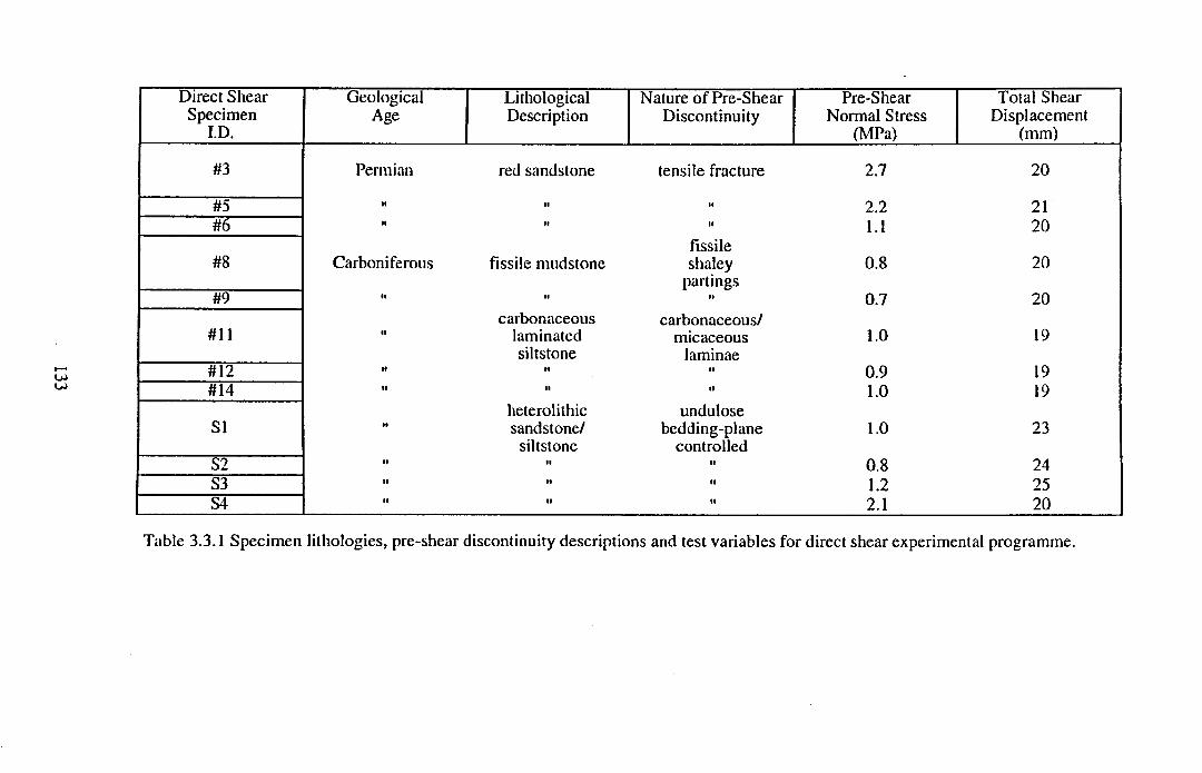
Direct Shear Specimen

ID .

GeologicalAge

LithologicalDescription

Nature of Pre-Shear Discontinuity

Pre-Shear Normal Stress

(MPa)

Total Shear Displacement

(mm)

#3 Permian red sandstone tensile fracture 2.7 20

#5 •1 il ll 2.2 21#6 M M ll

fissile1.1 20

#8 Carboniferous fissile mudstone shaleypartings

0.8 20

#9 ii it

carbonaceousii

carbonaceous/0.7 20

#11 II laminatedsiltstone

micaceouslaminae

1 . 0 19

#12 II II it 0.9 19#14 II II

heterolithicll

undulose1 . 0 19

SI il sandstone/siltstone

bedding-planecontrolled

1 . 0 23

S2 il ll ll 0.8 24S3 II II II 1.2 25S4 II ll II 2.1 20

Table 3.3.1 Specimen lithologies, pre-shear discontinuity descriptions and test variables for direct shear experimental programme.

Colour plates showing the lower and upper sliding surfaces of the twelve direct shear

specimens, taken post-testing, are presented in Appendix I. These photographs were taken

under oblique lighting, illuminating the surfaces from right to left, that is approximately

perpendicular to the direction of sliding, in order to highlight surface roughness and

topography. Arrows shown in each figure indicate the displacement direction of the lower

sliding surface (identified as the "BOT" sample) and the upper sliding surface (identified

as the "TOP" sample) as shown. Each specimen has been separated into lower and upper

halves about the shear plane so that, as photographed, the tops of the lower and upper

sliding surfaces were originally in contact, as were the right-hand-side o f the BOT-

surface and the left-hand-side of the TOP-surface. In this orientation, as illustrated, it is

informative to envisage the TOP-half being held rigid and stationary in its shear box,

whilst the BOT-half was displaced horizontally, with the resultant shear couple as

indicated.

From Appendix I the most striking feature that is immediately apparent on inspection, is

that all surfaces, to a greater or lesser extent, are liberally covered in sliding-induced

frictional wear debris. This shear debris can be considered as representing "genuine" fault

gouge, that is comminuted rock fragments liberated from the actual experimental sliding

surfaces due to the shearing action, as opposed to "artificial" fault gouge so often used in

laboratory experiments. The latter commonly consists of a layer of glass beads, clay

particles, crushed silica, or sampled natural fault gouge, placed between rigid rock or

steel platens which are subsequently sheared, so deforming the artificial gouge layer. One

principal advantage of conducting the direct shear testing programme under constant

norm al displacement conditions, has been that shear debris production has been

m axim ised (due to total suppression of dilatancy in favour of asperity shear) by

comparison with expected production under shearing modes o f constant normal stress or

stiffness. This has produced relatively large masses of shear debris, from a range of rock

types deformed under known boundary conditions, for analysis. Results from small

particle statistical analyses of these debris distributions, as well as correlations with

measured frictional strength parameters of the various sliding surfaces, are presented in

Chapter 6. In this section, qualitative descriptions of the various features observed on

134

sliding surfaces will be given, and an attempt made to characterise the different surface

morphologies that have evolved, in terms of lithological controls.

All the structural features observed on the sliding surfaces, regardless of the test

lithology, were attributed to brittle fracture and mechanical abrasion during frictional

sliding. The red sandstone specimens #3, #5 and #6 are shown in Fig.AI.l, Fig.AI.2 and

Fig.AI.3 respectively. All three samples show white patches of ground quartz grains,

easily discernible against the red background of the iron oxide-stained initial tensile

failure surfaces. These isolated patches of localised grain-size reduction show variable

areal extent, but always incomplete coverage of the sliding surfaces. Intuitively, the

surface distribution of the sheared patches and the location of the peak contact asperities

will be highly correlated. These regions of fault gouge are strongly striated with slip-

parallel linear features also recorded from natural fault surfaces, where they are

recognised as being the result of “asperity ploughing”, “debris streaking” and “erosional

sheltering” (Means, 1987)128.

A second feature immediately apparent on the surface o f the red sandstone shear planes,

takes the form of a planar structure showing a distinct resemblance to “slickensides” so

often noted from faults in the field (for a definition see Fleuty, 1975)1: ^. It has long been

known that these striations and step structures can be used for the determination of the

direction of movement along a fault, and prior to 1958 it was generally assumed that the

step-like protuberances faced in the direction of movement of the overriding surface

(Billings, 1954, p.149)130. However Paterson (1958)131 published a photograph of steps

developed on a shear surface formed during a triaxial test on Wombeyan marble which

clearly showed that the steps opposed the movement of the overriding surface. Paterson

concluded that movement directions along fault planes should not be determined only

from the attitude of the steps on the plane, but from other geological features as well. All

the slickensteps observed on both the BOT- and TOP- shear surfaces of red sandstone

specimens #3, #5 and #6 appeared to be incongruous, that is they faced against the

movement of the overriding block. Currently, two theories have been proposed to account

for this common facing direction. Gay (1970)*33, from experimental double shear testing

135

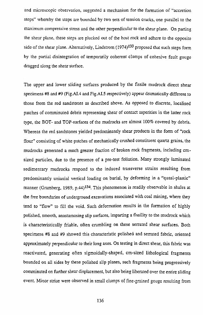
and microscopic observation, suggested a mechanism for the formation o f “accretion

steps’’ whereby the steps are bounded by two sets of tension cracks, one parallel to the

maximum compressive stress and the other perpendicular to the shear plane. On parting

the shear plane, these steps are plucked out of the host rock and adhere to the opposite

side of the shear plane. Alternatively, Lindstrom (1974)133 proposed that such steps form

by the partial disintegration of temporarily coherent clumps of cohesive fault gouge

dragged along the shear surface.

The upper and lower sliding surfaces produced by the fissile mudrock direct shear

specimens #8 and #9 (Fig.AI.4 and Fig.AI.5 respectively) appear dramatically different to

those from the red sandstones as described above. As opposed to discrete, localised

patches of comminuted debris representing shear of contact asperities in the latter rock

type, the BOT- and TOP-surfaces of the mudrocks are almost 100% covered by debris.

Whereas the red sandstones yielded predominantly shear products in the form of “rock

flour” consisting of white patches of mechanically crushed constituent quartz grains, the

mudrocks generated a much greater fraction of broken rock fragments, including cm-

sized particles, due to the presence of a pre-test foliation. Many strongly laminated

sedim entary mudrocks respond to the induced transverse strains resulting from

predominantly uniaxial vertical loading on burial, by deforming in a “quasi-plastic”

manner (Gramberg, 1989, p.44)134. This phenomenon is readily observable in shales at

the free boundaries of underground excavations associated with coal mining, where they

tend to “flow” to fill the void. Such deformation results in the formation o f highly

polished, smooth, anastamosing slip surfaces, imparting a fissility to the mudrock which

is characteristically friable, often crumbling on these serrated shear surfaces. Both

specimens #8 and #9 showed this characteristic polished and serrated fabric, oriented

approximately perpendicular to their long axes. On testing in direct shear, this fabric was

reactivated, generating often sigmoidally-shaped, cm-sized lithological fragments

bounded on all sides by these polished slip planes, such fragments being progressively

comminuted on further shear displacement, but also being liberated over the entire sliding

event. Minor striae were observed in small clumps of fine-grained gouge resulting from

136

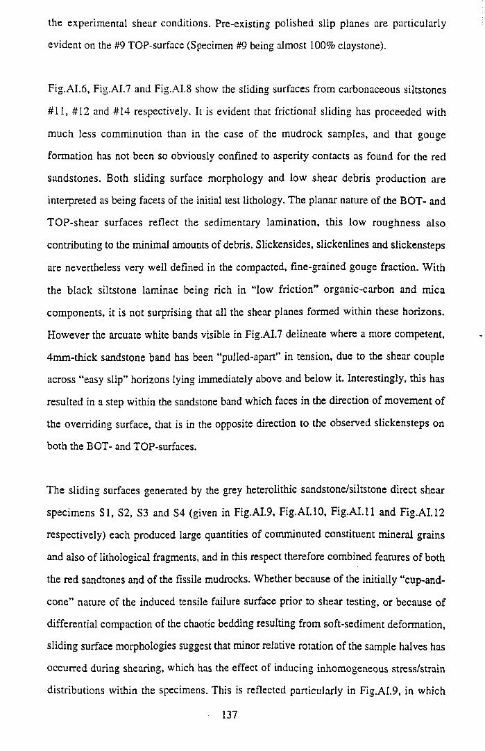
the experimental shear conditions. Pre-existing polished slip planes are particularly

evident on the #9 TOP-surface (Specimen #9 being almost 100% claystone).

Fig.AI.6, Fig.AI.7 and Fig.AI.8 show the sliding surfaces from carbonaceous siltstones

#11, #12 and #14 respectively. It is evident that frictional sliding has proceeded with

much less comminution than in the case of the mudrock samples, and that gouge

formation has not been so obviously confined to asperity contacts as found for the red

sandstones. Both sliding surface morphology and low shear debris production are

interpreted as being facets of the initial test lithology. The planar nature of the BOT- and

TO P-shear surfaces reflect the sedimentary lamination, this low roughness also

contributing to the minimal amounts of debris. Slickensides, slickenlines and slickensteps

are nevertheless very well defined in the compacted, fine-grained gouge fraction. With

the black siltstone laminae being rich in “low friction” organic-carbon and mica

components, it is not surprising that all the shear planes formed within these horizons.

However the arcuate white bands visible in Fig.AI.7 delineate where a more competent,

4mm-thick sandstone band has been “pulled-apart” in tension, due to the shear couple

across “easy slip” horizons lying immediately above and below it. Interestingly, this has

resulted in a step within the sandstone band which faces in the direction of movement of

the overriding surface, that is in the opposite direction to the observed slickensteps on

both the BOT- and TOP-surfaces.

The sliding surfaces generated by the grey heterolithic sandstone/siltstone direct shear

specimens SI, S2, S3 and S4 (given in Fig.AI.9, Fig.AI.10, F ig .A I.il and Fig.AI.12

respectively) each produced large quantities of comminuted constituent mineral grains

and also of lithological fragments, and in this respect therefore combined features of both

the red sandtones and of the fissile mudrocks. Whether because of the initially “cup-and-

cone” nature of the induced tensile failure surface prior to shear testing, or because of

differential compaction of the chaotic bedding resulting from soft-sediment deformation,

sliding surface morphologies suggest that minor relative rotation of the sample halves has

occurred during shearing, which has the effect of inducing inhomogeneous stress/strain

distributions within the specimens. This is reflected particularly in Fig.AI.9, in which

137

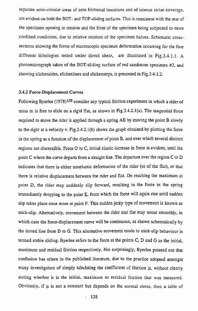
separate semi-circular areas of zero frictional lineations and of intense striae coverage,

are evident on both the BOT- and TOP-sliding surfaces. This is consistent with the rear of

the specimen opening in tension and the front of the specimen being subjected to more

confined conditions, due to relative rotation of the specimen halves. Schematic cross-

sections showing the forms of macroscopic specimen deformation occurring for the four

different lithologies tested under direct shear, are illustrated in Fig.3.4.1.1. A

photomicrograph taken of the BOT-sliding surface of red sandstone specimen #3, and

showing slickensides, slickenlines and slickensteps, is presented in Fig.3.4.1.2.

3.4.2 Force-Displacement Curves

Following Byerlee (1978)135 consider any typical friction experiment in which a rider of

mass m is free to slide on a rigid flat, as shown in Fig.3.4.2.1(a). The tangential force

required to move the rider is applied through a spring AB by moving the point B slowly

to the right at a velocity v. Fig.3.4.2.1(b) shows the graph obtained by plotting the force

in the spring as a function of the displacement of point B, and over which several distinct

regions are discernible. From O to C, initial elastic increase in force is evident, until the

point C where the curve departs from a straight line. The departure over the region C to D

indicates that there is either nonelastic deformation of the rider (or of the flat), or that

there is relative displacement between the rider and flat. On reaching the maximum at

point D, the rider may suddenly slip forward, resulting in the force in the spring

immediately dropping to the point E, from which the force will again rise until sudden

slip takes place once more at point F. This sudden jerky type of movement is known as

stick-slip. Alternatively, movement between the rider and flat may occur smoothly, in

which case the force-displacement curve will be continuous, as shown schematically by

the dotted line from D to G. This alternative movement mode to stick-slip behaviour is

termed stable sliding. Byerlee refers to the force at the points C, D and G as the initial,

maximum and residual friction respectively. Not surprisingly, Byerlee pointed out that

confusion has arisen in the published literature, due to the practice adopted amongst

many investigators of simply tabulating the coefficient of friction p., without clearly

stating whether it is the initial, maximum or residual friction that was measured.

Obviously, if p is not a constant but depends on the normal stress, then a table of

138

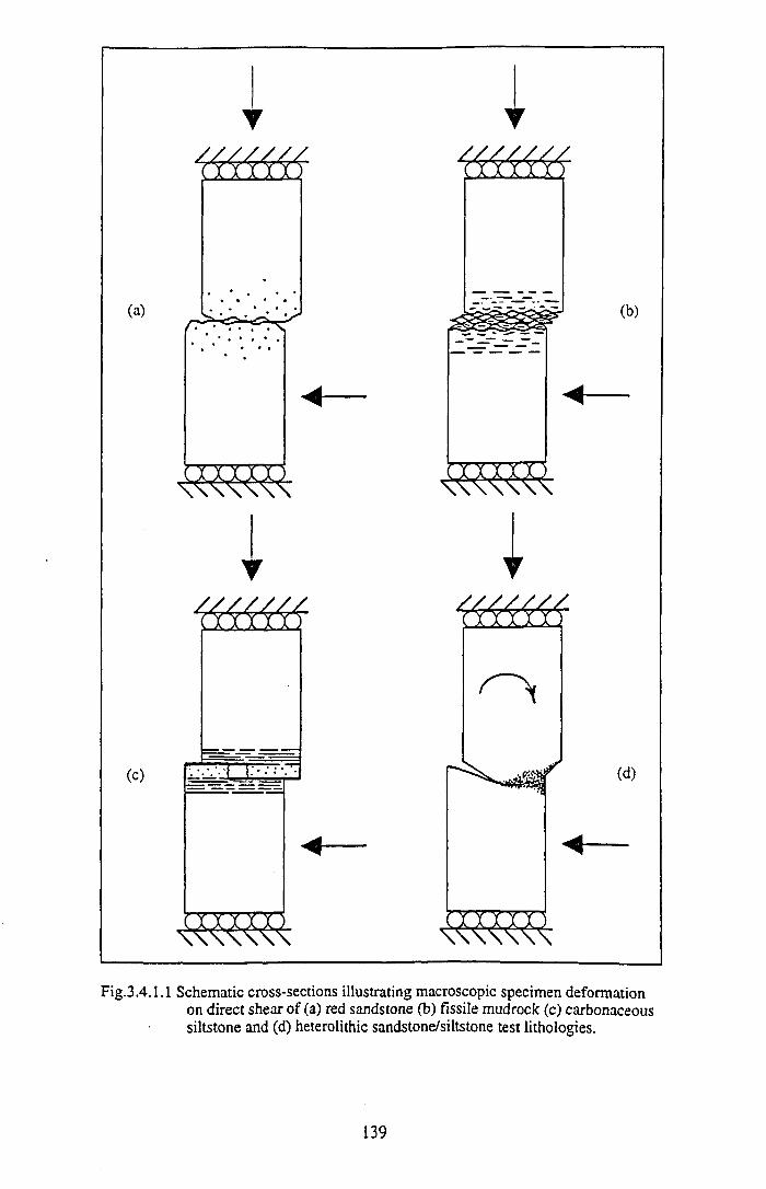
Fig.3.4.1.1 Schematic cross-sections illustrating macroscopic specimen deformation on direct shear of (a) red sandstone (b) fissile mudrock (c) carbonaceous siltstone and (d) heterolithic sandstone/siltstone test lithologies.

139

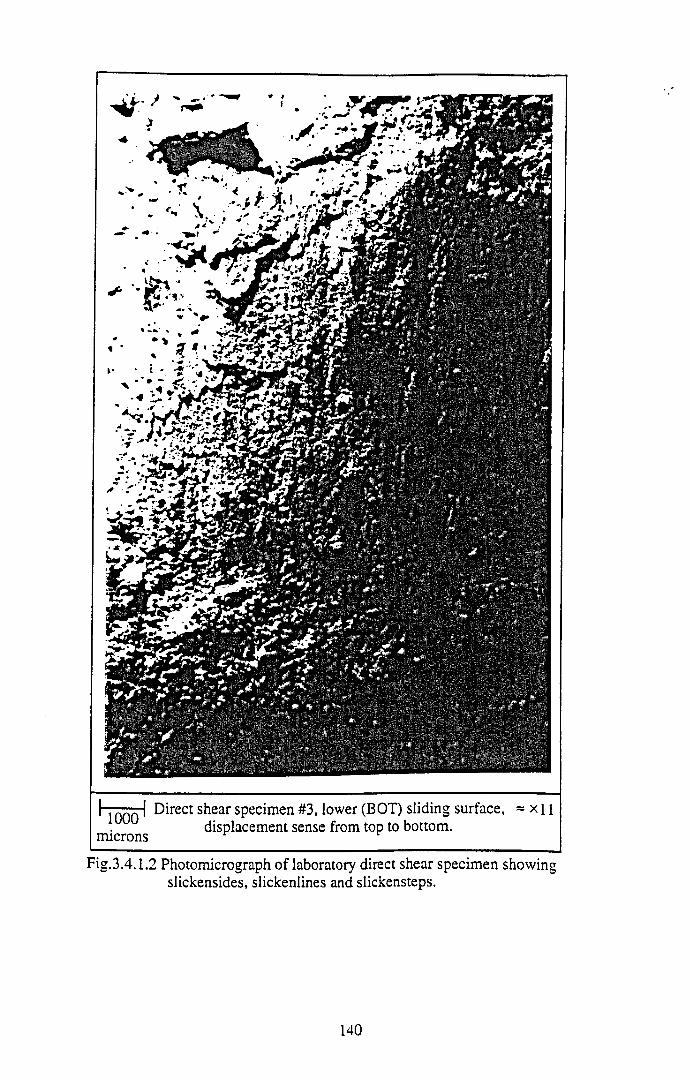
h I Direct shear specimen #3, lower (BOT) sliding surface, ~ x 1 1 displacement sense from top to bottom.

microns

Fig.3.4.1.2 Photomicrograph of laboratory direct shear specimen showing slickensides, slickenlines and slickensteps.

140

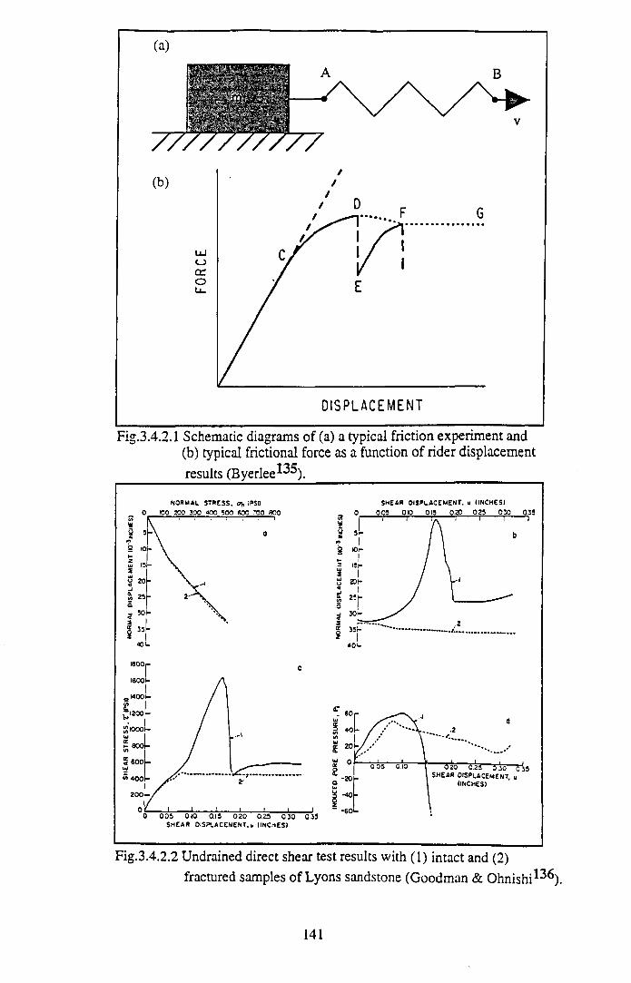
Fig.3.4.2.1 Schematic diagrams of (a) a typical friction experiment and(b) typical frictional force as a function of rider displacement results (Byerlee*35)

Fig.3.4.2.2 Undrained direct shear test results with (1) intact and (2)fractured samples of Lyons sandstone (Goodman & O hnishi*^).

141

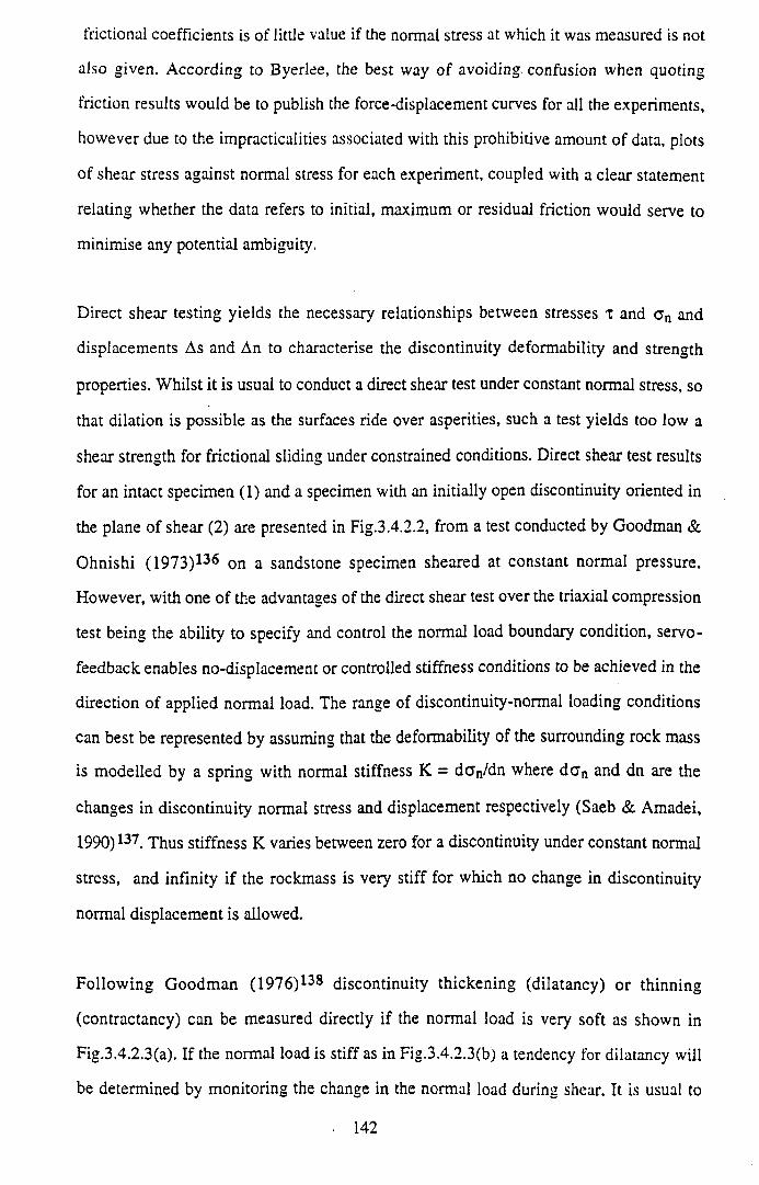
frictional coefficients is of little value if the normal stress at which it was measured is not

also given. According to Byerlee, the best way of avoiding, confusion when quoting

friction results would be to publish the force-displacement curves for all the experiments,

however due to the impracticalities associated with this prohibitive amount of data, plots

of shear stress against normal stress for each experiment, coupled with a clear statement

relating whether the data refers to initial, maximum or residual friction would serve to

minimise any potential ambiguity.

Direct shear testing yields the necessary relationships between stresses t and c n and

displacements As and An to characterise the discontinuity deformability and strength

properties. Whilst it is usual to conduct a direct shear test under constant normal stress, so

that dilation is possible as the surfaces ride over asperities, such a test yields too low a

shear strength for frictional sliding under constrained conditions. Direct shear test results

for an intact specimen (1) and a specimen with an initially open discontinuity oriented in

the plane of shear (2) are presented in Fig.3.4.2.2, from a test conducted by Goodman &

Ohnishi (1973)136 on a sandstone specimen sheared at constant normal pressure.

However, with one of the advantages of the direct shear test over the triaxial compression

test being the ability to specify and control the normal load boundary condition, servo-

feedback enables no-displacement or controlled stiffness conditions to be achieved in the

direction of applied normal load. The range of discontinuity-normal loading conditions

can best be represented by assuming that the deformability of the surrounding rock mass

is modelled by a spring with normal stiffness K = d a n/dn where d c n and dn are the

changes in discontinuity normal stress and displacement respectively (Saeb & Amadei,

1990) 137. Thus stiffness K varies between zero for a discontinuity under constant normal

stress, and infinity if the rockmass is very stiff for which no change in discontinuity

normal displacement is allowed.

Following Goodman (1976)138 discontinuity thickening (dilatancy) or thinning

(contractancy) can be measured directly if the normal load is very soft as shown in

Fig.3.4.2.3(a). If the normal load is stiff as in Fig.3.4.2.3(b) a tendency for dilatancy will

be determined by monitoring the change in the normal load during shear. It is usual to

142

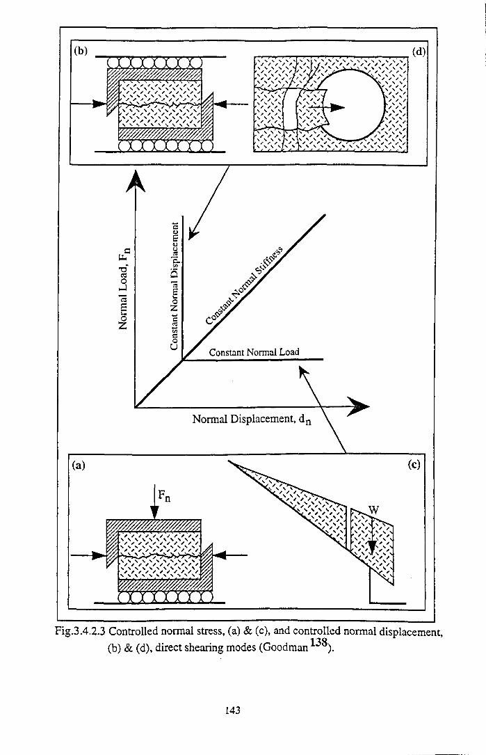
143

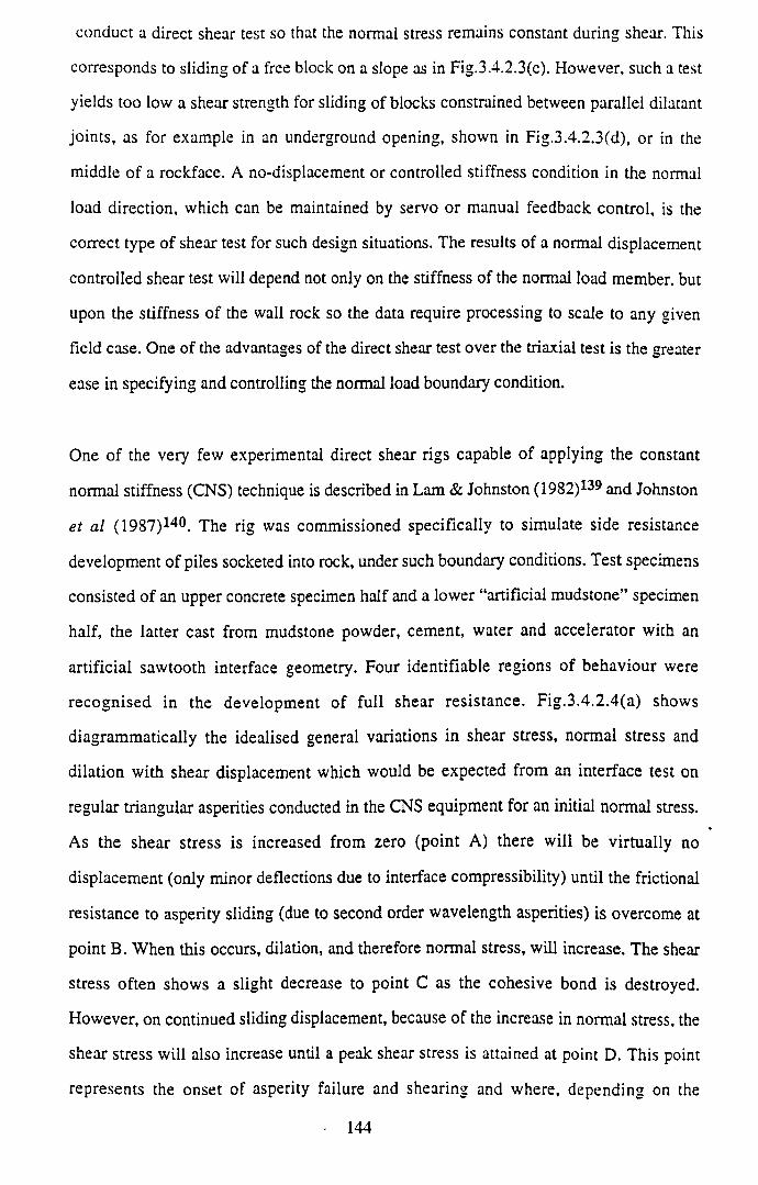
conduct a direct shear test so that the normal stress remains constant during shear. This

corresponds to sliding of a free block on a slope as in Fig.3.4.2.3(c). However, such a test

yields too low a shear strength for sliding of blocks constrained between parallel dilatant

joints, as for example in an underground opening, shown in Fig.3.4.2.3(d), or in the

middle of a rockface. A no-displacement or controlled stiffness condition in the normal

load direction, which can be maintained by servo or manual feedback control, is the

correct type of shear test for such design situations. The results of a normal displacement

controlled shear test will depend not only on the stiffness of the normal load member, but

upon the stiffness of the wall rock so the data require processing to scale to any given

field case. One of the advantages of the direct shear test over the triaxial test is the greater

ease in specifying and controlling the normal load boundary condition.

One of the very few experimental direct shear rigs capable of applying the constant

normal stiffness (CNS) technique is described in Lam & Johnston (1982)139 and Johnston

et al (1987)140. The rig was commissioned specifically to simulate side resistance

development of piles socketed into rock, under such boundary conditions. Test specimens

consisted of an upper concrete specimen half and a lower “artificial mudstone” specimen

half, the latter cast from mudstone powder, cement, water and accelerator with an

artificial sawtooth interface geometry. Four identifiable regions of behaviour were

recognised in the development of full shear resistance. Fig.3.4.2.4(a) shows

diagrammatically the idealised general variations in shear stress, normal stress and

dilation with shear displacement which would be expected from an interface test on

regular triangular asperities conducted in the CNS equipment for an initial normal stress.

As the shear stress is increased from zero (point A) there will be virtually no

displacement (only minor deflections due to interface compressibility) until the frictional

resistance to asperity sliding (due to second order wavelength asperities) is overcome at

point B. When this occurs, dilation, and therefore normal stress, will increase. The shear

stress often shows a slight decrease to point C as the cohesive bond is destroyed.

However, on continued sliding displacement, because of the increase in normal stress, the

shear stress will also increase until a peak shear stress is attained at point D. This point

represents the onset of asperity failure and shearing and where, depending on the

144

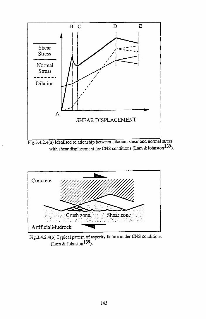
B C D

SHEAR DISPLACEMENT

Fig.3.4.2.4(a) Idealised relationship between dilation, shear and norma. stress13%with shear displacement for CNS conditions (Lam &Johnston )

Fig.3.4.2.4(b) Typical pattern of asperity failure under CNS conditions (Lam & Johnston*^).

145

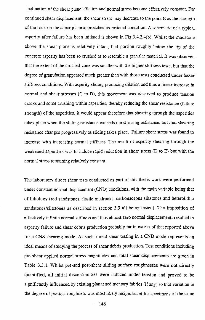
inclination of the shear plane, dilation and normal stress become effectively constant. For

continued shear displacement, the shear stress may decrease to the point E as the strength

of the rock on the shear plane approaches its residual condition. A schematic of a typical

asperity after failure has been initiated is shown in Fig.3.4.2.4(b). Whilst the mudstone

above the shear plane is relatively intact, that portion roughly below the tip of the

concrete asperity has been so crushed as to resemble a granular material. It was observed

that the extent of the crushed-zone was smaller with the higher stiffness tests, but that the

degree of granulation appeared much greater than with those tests conducted under lesser

stiffness conditions. With asperity sliding producing dilation and thus a linear increase in

normal and shear stresses (C to D), this movement was observed to produce tension

cracks and some crushing within asperities, thereby reducing the shear resistance (failure

strength) of the asperities. It would appear therefore that shearing through the asperities

takes place when the sliding resistance exceeds the shearing resistance, but that shearing

resistance changes progressively as sliding takes place. Failure shear stress was found to

increase with increasing normal stiffness. The result of asperity shearing through the

weakened asperities was to induce rapid reduction in shear stress (D to E) but with the

normal stress remaining relatively constant.

The laboratory direct shear tests conducted as part of this thesis work were performed

under constant normal displacement (CND) conditions, with the main variable being that

of lithology (red sandstones, fissile mudrocks, carbonaceous siltstones and heterolithic

sandstones/siltstones as described in section 3.3 all being tested). The imposition of

effectively infinite normal stiffness and thus almost zero normal displacement, resulted in

asperity failure and shear debris production probably far in excess of that reported above

for a CNS shearing mode. As such, direct shear testing in a CND mode represents an

ideal means of studying the process of shear debris production. Test conditions including

pre-shear applied normal stress magnitudes and total shear displacements are given in

Table 3.3.1. W hilst pre-and post-shear sliding surface roughnesses were not directly

quantified, all initial discontinuities were induced under tension and proved to be

significantly influenced by existing planar sedimentary fabrics (if any) so that variation in

the degree of pre-test roughness was most likely insignificant for specimens o f the same

146

lithology, but probably high from rock type to rock type. The greatest unavoidable

between-sample variable for test specimens sourced from the same rock type, was

probably sliding velocity, which may have varied by up to a factor of two in the most

extreme case, as a result of manual control of horizontal actuator displacement.

Force-displacement curves for the direct shear (CND) test programme are given in

Fig.3.4.2.5 to Fig.3.4.2.8. Force-displacement curves for red sandstone specimens #3, #5

and #6 are presented in Fig.3.4.2.5(a) to (c) respectively. Maximum shear and normal

loads for #5 are more than twice those of #3 and #6, despite the lithology being broadly

homogeneous on a specimen-scale, and the pre-shear normal load for #5 being

intermediate between that of #3 and #6. This could be a result of specimen #5 possessing

a rougher sliding surface, as it appears to have produced the greatest amounts of large

fragm ent-sized wear products (Fig.AI.2). Specimens #3 and #5 show several

complementary peaks in their shear and normal load profiles, followed by sudden stress

drops, such jerky fluctuations as particularly exemplified by #3, probably representing

dynamic failure of relatively large-wavelength asperities. Specimen #6, which shows

gradual increases in both shear and normal load to broad plateau’s, is seen to produce a

post-test sliding surface morphology characterised by minimal damage confined to small

isolated patches of crushed grains, corresponding to areas of asperity contact. Small-scale

jerky fluctuations in the shear load profile for #6 are interpreted as stick-slip oscillations,

which are often associated in the literature (see Jaeger & Cook8 p61) with frictional

sliding on relatively smoother shear planes. The fissile mudrock specimens #8 and #9

record markedly different load-displacement curves (Fig.3.4.2.6(a) and (b) respectively)

to those of the red sandstones. Both specimens exhibit synchronous peak normal and

shear loads, occurring at exactly the same sliding displacement. Specimen #8 shows shear

and normal load profiles which are almost symmetrical, with the pre-peak and post-peak

parts o f each curve being almost mirror images about the peaks. However #9 exhibits

load-displacement curves reminiscent of red sandstone #3, with pre-peak variations

suggestive of asperity failure. Carbonaceous siltstones #11, #12 and #14 (Fig.3.4.2.7(a) to

(c) respectively) all show similar load-displacement profiles characterised by broadly

linear increases in normal and shear loads with sliding displacement up to peak values,

147

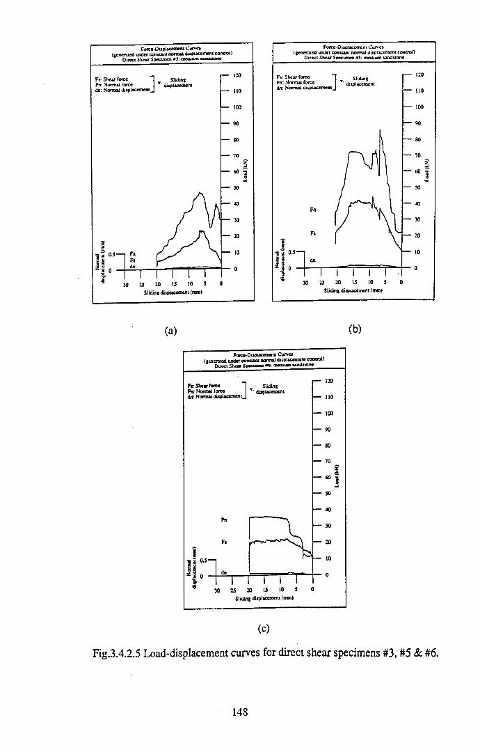
(a) (b)

(c)

Fig.3.4.2.5 Load-displacement curves for direct shear specimens #3, #5 & #6.

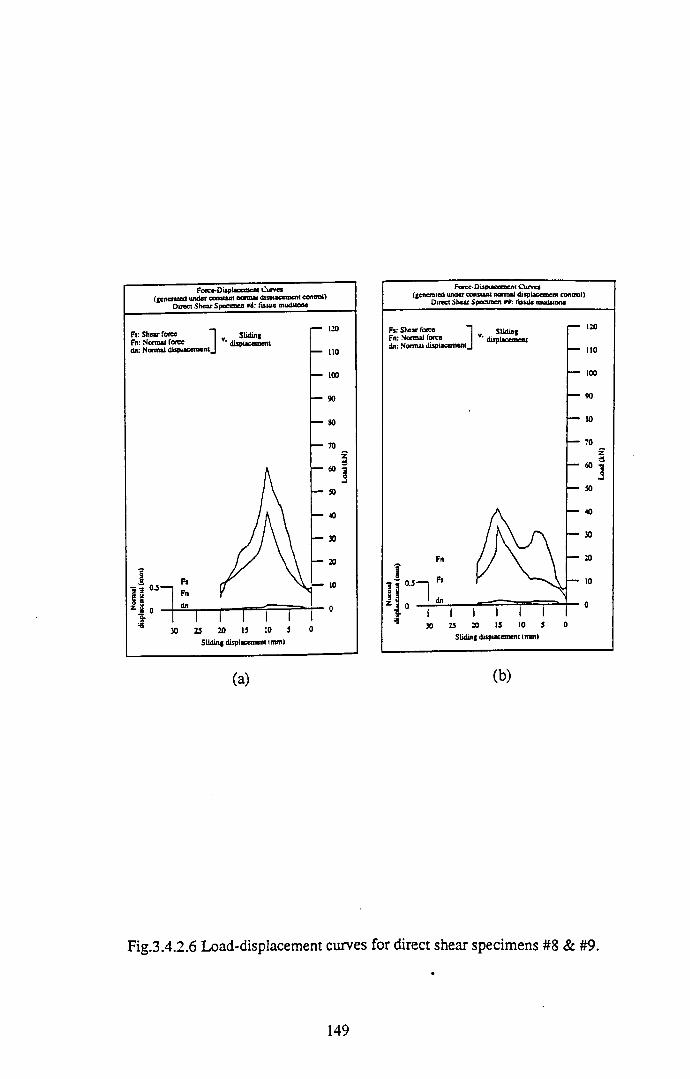
Fig.3.4.2.6 Load-displacement curves for direct shear specimens #8 & #9.

149

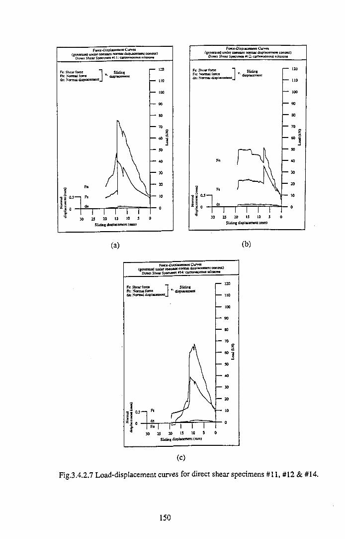
(C)

Fig.3.4.2.7 Load-displacement curves for direct shear specimens #11, #12 & #14.

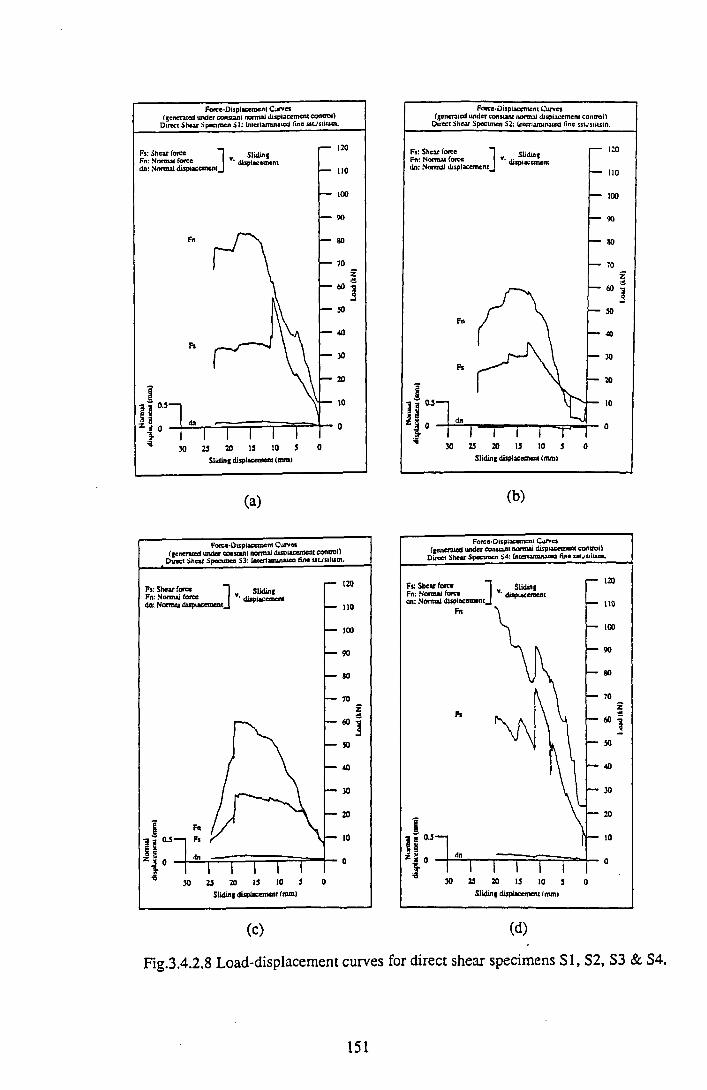
(a) (b)

Fig.3.4.2.8 Load-displacement curves for direct shear specimens SI, S2, S3 & S4.

151

followed by sudden, large magnitude vertical drops which may well signify the failure of

more competent laminae through “puiling-apart” in tension. Finally, heterolithic

specimens S I, S2, S3 and S4 (Fig.3.4.2.8(a) to (d) respectively) show a wide range in

force-displacement curves, reflecting presumably the wider variability in their percentage

mineral composition and discontinuity surface roughness. Relatively larger variation in

normal displacement (up to around 0.2mm) than recorded for the other lithologies may

well reflect rotation of the upper specimen half as illustrated in Fig.3.4 .1.1(d).

3.4.3 Theoretical Analysis of Contact A rea Variation W ith Sliding Displacement

In order to convert the normal and shear load profiles as presented above, into variations

in normal and shear stress magnitude with shear displacement, it is necessary to know

the discontinuity sliding surface area across and along which, respectively, the normal

and shear stresses have acted. Whilst, to a first order approximation, the cross-sectional

area of the cylindrical specimen might suffice, such an assumption ignores variation in

upper and lower specimen half contact area with sliding displacement, and thus tends to

underestimate stress magnitudes. Ideally, variation in asperity contact area with slip is

required, however this is difficult to evaluate experimentally without unloading the

specimen, and is even more complex for specimens generating a large volume of

comminuted rock debris. Instead, a theoretical analysis was undertaken to determine the

area of overlap of two circles (representing the upper and lower direct shear specimen

halves) with varying centre displacement. Consider the geometry depicted in Fig.3.4.3.1

in which a circle o f equation x2 + y 2 = r2 with centre O on the origin, has suffered a

translation in the x-direction to a new position with centre X. This translation, s, is

equivalent to sliding displacement. No displacement is experienced in the y-direction.

The Cartesian-coordinates of the points indicated in Fig.3.4.3.1 are thus: 0 (0 , 0); l(s-r,

0); 2(s/2, 0); 3(r, 0) and 4(s, 0). With the point of contact between the two circumferences

being given by y=(r2 - x2) 1/2dx, the shaded area as shown in Fig.3.4.3.1 and representing

one-quarter of the total area of overlap is given by:

152

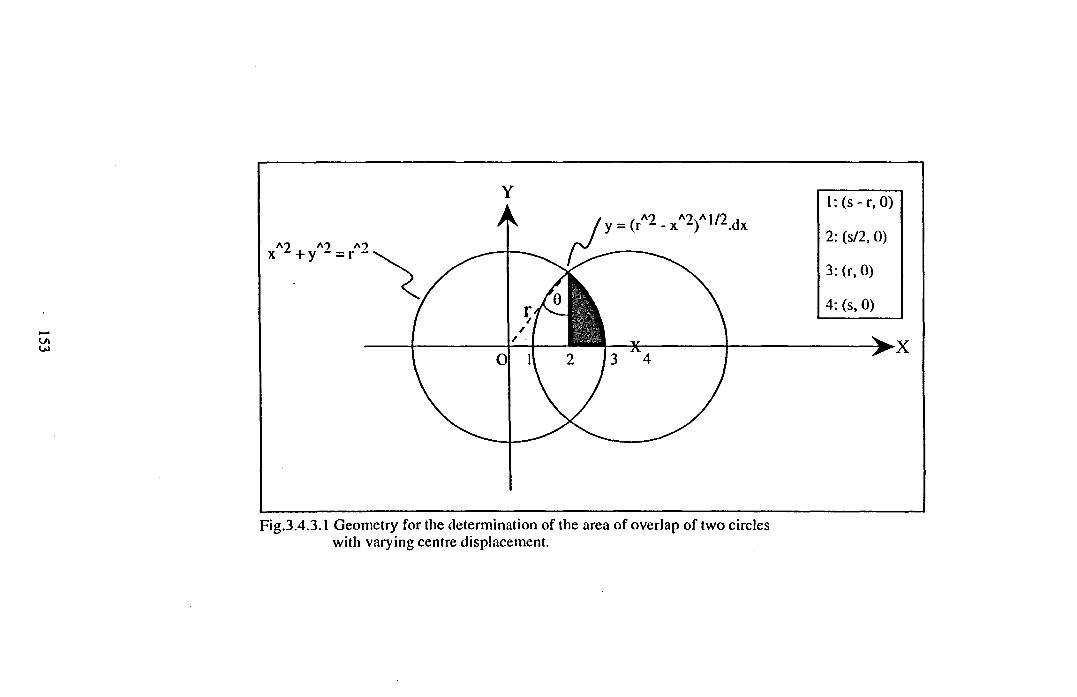
Fig.3.4.3.1 Geometry for the determination of the area of overlap of two circles with varying centre displacement.

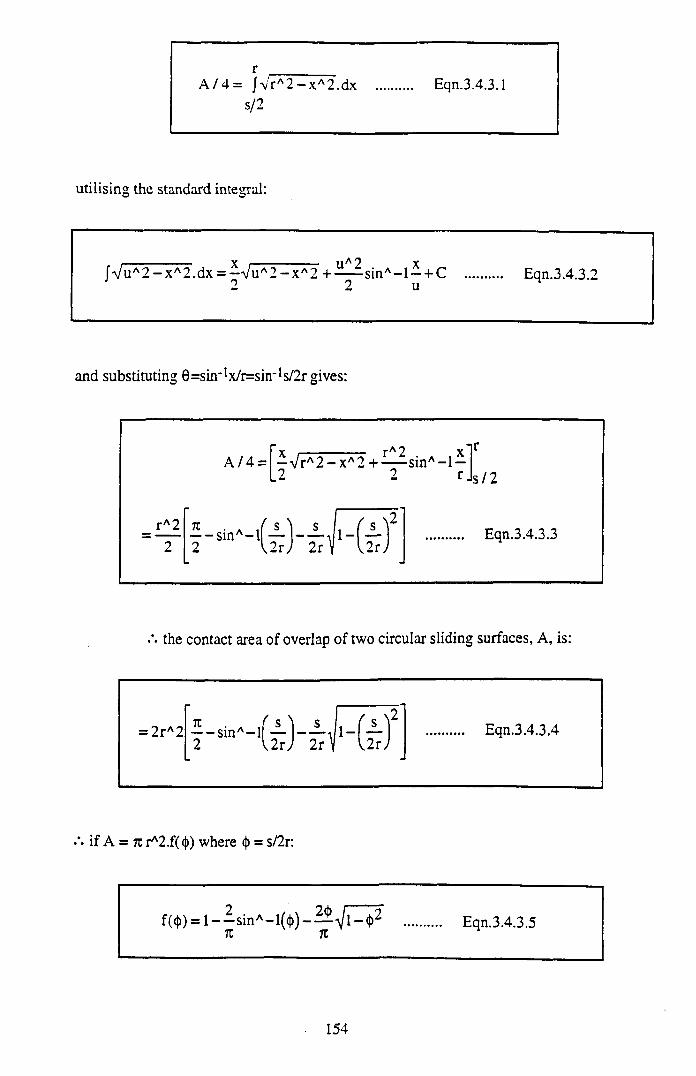
rA / 4 = JVrA2 - x A2.dx .... Eqn. 3.4.3.1

s/2

utilising the standard integral:

JVuA2 - x A2.dx = —VuA2 - x A2 + -^-^sinA- l — + C 1 2 2 u

Eqn.3.4.3.2

and substituting 0=sin‘1x/r=sin’1s/2r gives:

the contact area of overlap of two circular sliding surfaces, A, is:

Eqn.3.4.3.4

if A = k rA2.f( <|)) where <|) = s/2r:

f(<t>) = 1 - - s i n A -1((|))7C Tt

Eqn.3.4.3.5

154

when s = 0, that is for complete overlap <f) = 0 and f(<|)) = 1 A = rcrA2, and when s = 2r,

that is for zero overlap (j) = 1 and f(<f>) = 0 A = 0.

Thus by using Eqn.3.4.3.4, slip-dependent contact areas can be calculated for more

accurate quantification of stress magnitudes from measured shear and normal load

profiles. For a shear displacement of 20mm, as routinely applied to the majority of the

direct shear specimens described here, contact area has decreased to around 78% of that

corresponding to zero offset.

3.4.4 Stress - displacement curves

Utilising the theoretical variation in contact area with shear displacement relationship

presented in section 3.4.3, the load versus displacement plots given in section 3.4.2 were

converted to stress versus sliding profiles. Individual load values were manually read at

1mm shear displacement increments, directly from the shear and normal load plots for

the twelve direct shear specimens. These values were then entered into a Microsoft®

Excel spreadsheet and divided by the appropriate “slip-corrected” contact areas. Thus the

normal and shear stress versus sliding displacement plots were generated, as presented in

Fig.3.4.4.1 (red sandstones) Fig.3.4.4.2 (fissile mudrocks) Fig.3.4.4.3 (carbonaceous

siltstones) and Fig.3.4.4.4 (heterolithics). These plots also present stress profiles

calculated using a contact area equivalent to the specimen cross-sectional area (initial

diameter of core = 118mm a 10936mm2) thus ignoring any variation with shearing.

From comparison of the constant and variable contact area stress profiles, it is readily

apparent that consideration of a sliding surface area which changes with shear

displacement, produces markedly different results from those generated under the

assumption of constant contact area.

3.5 EM PIRICA L EXPRESSIONS FO R FRICTIONAL STRENGTH

In defining Amonton’s 141 law (see for example Jaeger & Cook8 pp.53-54) suppose that

two bodies with an approximately plane surface of contact of apparent area A are pressed

together by force W normal to the plane of contact, and the shear force F parallel to the

155

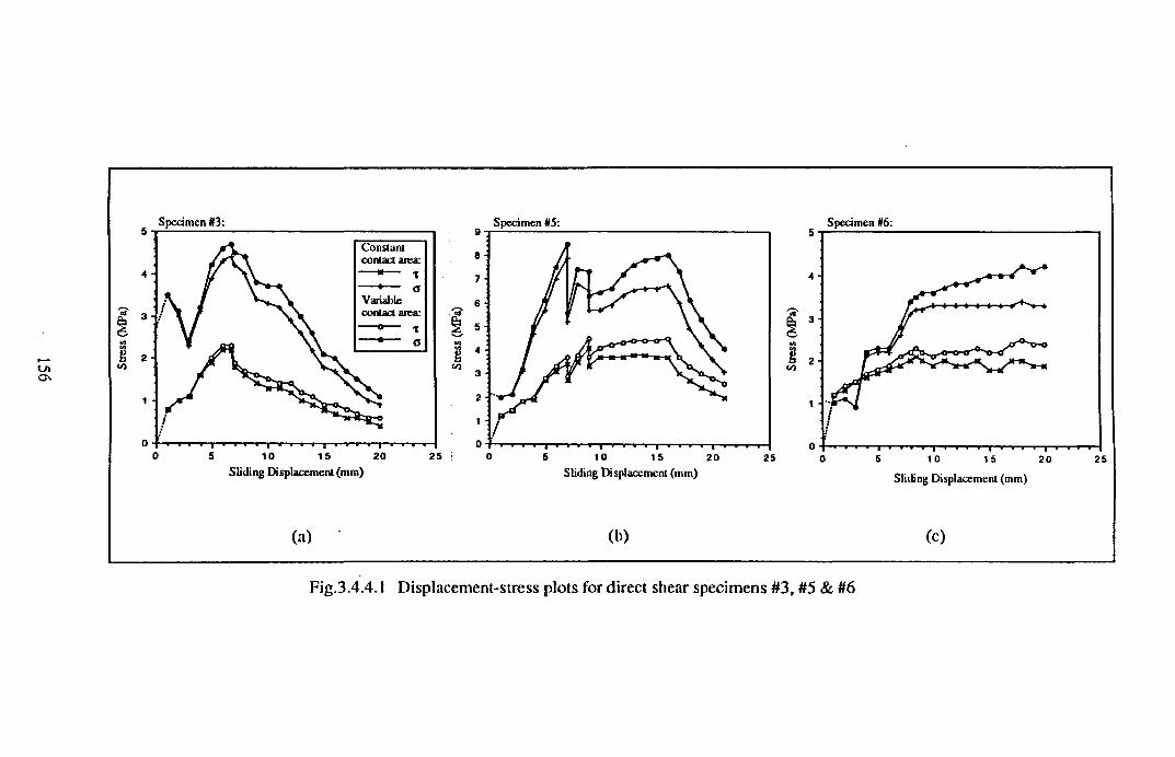
(a) (b) (c)

Fig.3.4.4.1 Displacement-stress plots for direct shear specimens #3, #5 & #6

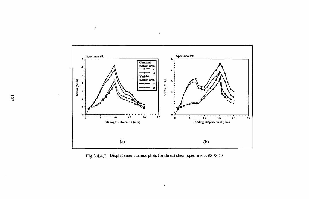
Sp ec im e n #8: Sp ec im e n #9:

U\-J

(a) (b)

Fig.3.4.4.2 Displacement-stress plots for direct shear specimens #8 & #9

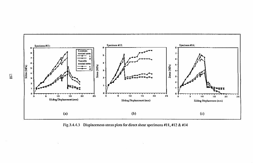
Sp ec im e n N 12: Spec im en #14:

(a) (b) (c)

Fig.3.4.4.3 Displacement-stress plots for direct shear specimens #11, #12 & #14

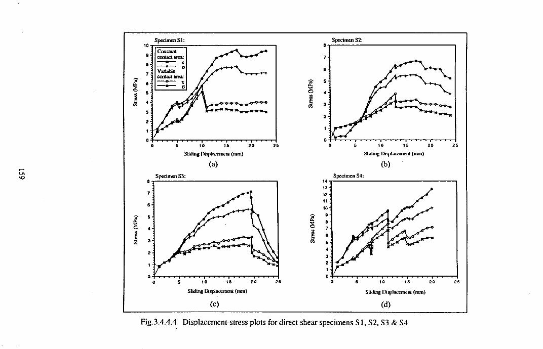
Spec im en S I :

(a)

Spec im en S2 :

(b)Specimen S3: Specimen S4:

(C) (d)

Fig.3.4.4.4 Displacement-stress plots for direct shear specimens S 1, S2, S3 & S4

surface of contact necessary to initiate sliding on it is measured. The relationship

between F and W is thus expressed as:

F = |i*.W .......... Eqn.3.5.1

where |i* is called the coefficient of friction and is dependent on the nature of the

materials and the finish and state of the surfaces in contact. This relation is known as

Amonton’s law, in which division of Eqn.3.5.1 by A yields:

T=|i*.cr .......... Eqn.3.5.2

where a is the normal stress across the surfaces in contact and x the shear stress necessary

to initiate sliding. It is important to note that an asterisk superscript is here employed

specifically to indicate a frictional coefficient defined as the ratio of t to a , that is by

Amonton's law as given in Eqn.3.5.2, and should not be confused with various other

frictional constants (also designated by |i , but without the asterisk superscript) associated

with different criteria for sliding. Jaeger & Cook make the important acknowledgement

that understanding of frictional phenomena is derived largely from the work of Bowden

and his co-workers based on the study of metals, Bowden and Tabor (1950)142,

(1964)143. The adhesion theory of friction proposed by Bowden, Moore and Tabor

(1943)144 to explain the frictional resistance developed between metal surfaces,

postulates that the very great adhesive forces at asperity contacts result in cold welding at

these junctions, so that the frictional resistance developed is equal to the product of the

real area of contact and the shear strength of the metal junctions. Indeed, at these

junctions the contact appears to be so intimate that the metals became welded together,

with the initiation of sliding requiring the shearing through of these welded contacts. This

theory leads to the relationship described by Eqn.3.5.2, and thus Amonton’s law is

qualitatively explained. However, the situation is probably more complex in reality than

that described by the above theory, for example a large number of asperities will exhibit a

160

wide range of contact loads, so that deformation at some may be elastic whilst others may

be deforming plastically. Archard (1958)145 has discussed such details of the frictional

sliding process more completely, and concluded that the law of friction was perhaps best

expressed by the power relationship:

F = |i.W m .......... Eqn.3.5.3

where 2/3 m 1. The specific case of m=2/3 corresponds to purely elastic deformation in

which the area of contact is proportional to w 2''3.

W hilst the above defined adhesion theory of friction, with much of it having been

checked empirically, appears admissible for sliding of metallic interfaces, it is of doubtful

validity for rocks and minerals, because most minerals tend to fail by brittle fracture

rather than by plastic flow, and the welding postulated for metals may not hold for

minerals. The concept of contact at a limited number of asperities does, however, remain

valid for geomaterials, although as yet no adequate theory of their behaviour has been

forwarded. Initial study along such lines was instigated by Byerlee (1967)146 who

proposed a simple theory of friction based on tensile brittle fracture, as a more realistic

alternative to the classic adhesion theory developed for metals. In Byerlee’s model the

surfaces were assumed to touch at the peaks of asperities, and sliding to occur when the

asperities failed by brittle fracture. The frictional coefficient, ]i*, was defined as the ratio

of the shear force required to cause sliding to the applied normal force across the

surfaces. For the postulation of brittle asperity failure rather than plastic shear, the

characterising brittle failure criterion was taken as low tensile strength, thus it was

assumed that the stress to produce brittle fracture in tension was much less than the stress

to produce plastic shear. Byerlee investigated a unique relation between the forces

required to break off the tips of the asperities, by analysing certain ideal asperity shapes.

Using a truncated cone as an asperity model, and assuming it to fail in tension, Byerlee

deduced that Amonton's law should hold for such a geometry, with a small value of p* of

the order of 0.1. For experiments approximating closely to this ideal brittle friction

161

model, p* was found to be very close to 0.1, even for materials such as quartz and caicite

with widely differing strengths. The character of wear particles produced during sliding

and the way in which p* was seen to depend on normal load, roughness and environment

all tended to support Byerlee’s model of friction based on brittle fracture of asperities as

opposed to one involving plastic shear deformation. Byerlee attributed the fact that higher

values are commonly measured to the interlocking of asperities. As well as small-scale

tensile failure of asperities, the extended shear discontinuities that occur in rockmasses

including hydrocarbon reservoirs show irregular surface roughness, so that the effects of

asperity ploughing and inclined sliding may be expected to occur. In Table 3.5.1 a

summary of empirical and theoretical frictional strength criteria for rock discontinuities,

as compiled from the rock mechanical literature, is presented. No derivation or discussion

of individual criteria are given here, as these can be gained from the appropriate

references. However, what is immediately apparent from Table 3.5.1, is the wide range of

empirically derived constants utilised by the various criteria.

The resistance to sliding at an interface is usually expressed in terms of a coefficient of

friction, p*, defined as the ratio of the shear force to normal force which is necessary

either to initiate sliding (the coefficient of "static", "stationary" or "starting" friction) or to

maintain continuing sliding (the coefficient of "dynamic", "kinetic" or "sliding" friction).

This coefficient p.*, as defined by Amonton's law (Eqn.3.5.2) was designated the

"variable" coefficient of friction by Jaeger (1959)147, whilst Donath et al (1972)157

referred to it as the "idealised" coefficient of friction. Paterson9 noted that even under

given conditions, unique values cannot in general be given for the coefficients of friction,

especially of dynamic friction, because of change in the frictional resistance with the

amount of sliding. This change occurs because, in most studies on rock friction, two

relatively large surfaces are moved over each other by amounts that are usually much less

than the linear dimensions of the surfaces, and the average normal stresses are such that

considerable wear or surface damage occurs during the sliding, affecting the resistance to

further sliding. It is clear that both the evolving sliding surface morphology and the

progressive production of fragmented rock debris play integral roles in determining the

162

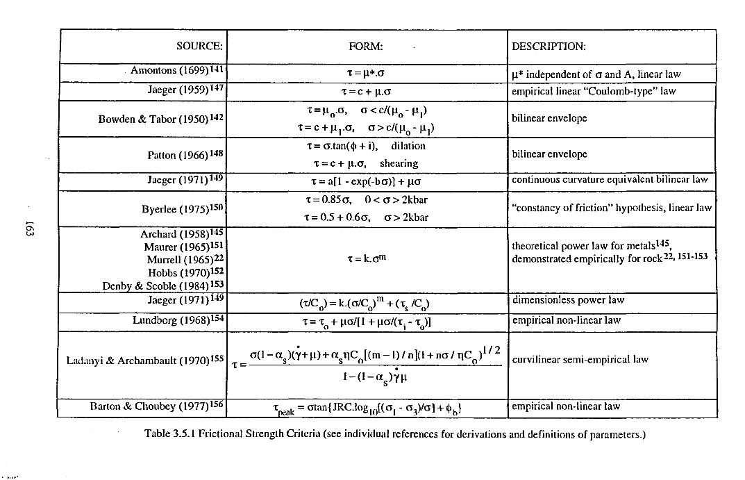
SOURCE: FORM: DESCRIPTION:

Amontons (1699)141 t = p * . a H* independent of a and A, linear lawJaeger (1959) I47 X = C + | i . 0 empirical linear “Coulomb-type” law

Bowden & Tabor (1950)142x = n o . a , o < c / ( | i o - (ij)

x = c + n , . a , a > c / ( n o - n , )bilinear envelope

Patton (1966)148x= a.tan(<|> + i), dilation

x = c + fi.a, shearingbilinear envelope

Jaeger(1971)149 x = a[ 1 - exp(-ba)] + continuous curvature equivalent bilinear law

Byerlee (1975)15°x = 0.85 a, 0 < a > 2kbar

x = 0.5 + 0.60 , 0 > 2kbar“constancy of friction” hypothesis, linear law

Archard (1958)145 Maurer (1965)151Murrell (1965)22 Hobbs (1970)152

Denby & Scoble (1984)153

x = k.omtheoretical power law for metals*45, demonstrated empirically for rock22,151-153

Jaeger (1971)149 (x/C0) = k.(a/Co)m + (xs /Co) dimensionless power law

Lundborg (1968)154 x = x o + pa/[l + p a /(x r xQ)] empirical non-linear law

Ladanyi & Archambault (1970)155 0 ( 1 - a s )(y + F) + « silCo [(m - 1) / n](l + na / x\Co )112 curvilinear semi-empirical law

l - 0 - a s )Ylt

Barton & Choubey (1977)156 W = otan{ JRC.log10[(o , - o 3)/o] + empirical non-linear law

Table 3.5.1 Frictional Strength Criteria (see individual references for derivations and definitions of parameters.)

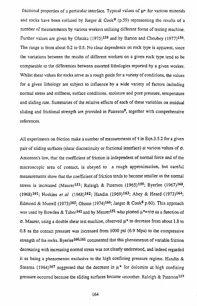
frictional properties of a particular interface. Typical values of p* for various minerals

and rocks have been collated by Jaeger & Cook8 (p.59) representing the results of a

number of measurements by various workers utilising different forms of testing machine.

Further values are given by Ohnaka (1975)158 and by Barton and Choubey (1977)156.

The range is from about 0.2 to 0.8. No clear dependence on rock type is apparent, since

the variations between the results of different workers on a given rock type tend to be

comparable to the differences between assorted lithologies reported by a given worker.

Whilst these values for rocks serve as a rough guide for a variety of conditions, the values

for a given lithology are subject to influence by a wide variety of factors including

normal stress and stiffness, surface conditions, moisture and pore pressure, temperature

and sliding rate. Summaries of the relative effects of each of these variables on residual

sliding and frictional strength are provided in Paterson9, together with comprehensive

references.

All experiments on friction make a number of measurements of x in Eqn.3.5.2 for a given

pair of sliding surfaces (shear discontinuity or frictional interface) at various values of a.

Amonton's law, that the coefficient of friction is independent of normal force and of the

m acroscopic area of contact, is obeyed to a rough approximation, but careful

measurements show that the coefficient of friction tends to become smaller as the normal

stress is increased (M aurer151; Raleigh & Paterson (1965)159; Byerlee (1967)160,

( 1968) 16!; Hoskins et al (1968)162; Handin (1969)163; Abey & Heard (1973)164;

Edmond & Murrell (1973)165; Olsson (1974)166; Jaeger & Cook8 p.60). This approach

was used by Bowden & Tabor142 and by Maurer151 who plotted fi*='C/a as a function of

a . Maurer, using a double shear test machine, observed p* to decrease from about 1.8 to

0.8 as the contact pressure was increased from 1000 psi (6.9 Mpa) to the compressive

strength of the rocks. Byerlee160»161 commented that this phenomenon of variable friction

decreasing with increasing normal stress was not clearly understood, and indeed regarded

it as being a phenomenon exclusive to the high confining pressure regime. Handin &

Stearns (1964)167 suggested that the decrease in p.* for dolomite at high confining

pressure occurred because the sliding surfaces became smoother. Raleigh & Paterson159

164

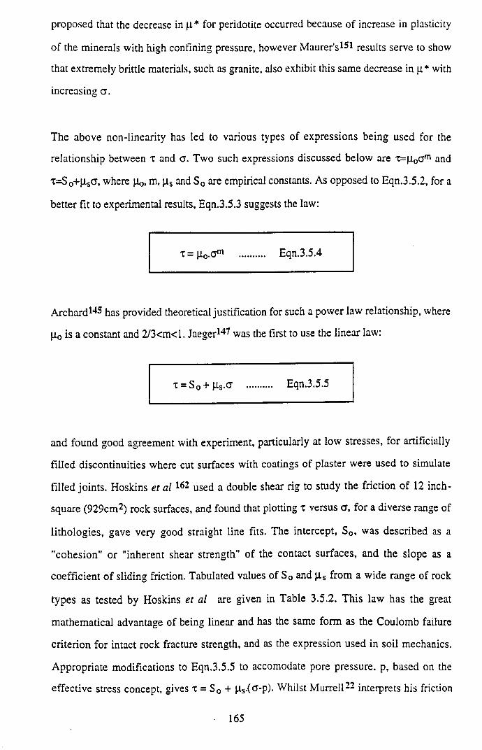
proposed that the decrease in |i* for peridotite occurred because of increase in plasticity

of the minerals with high confining pressure, however Maurer’s151 results serve to show

that extremely brittle materials, such as granite, also exhibit this same decrease in with

increasing a .

The above non-linearity has led to various types of expressions being used for the

relationship between x and a . Two such expressions discussed below are T=(i0o m and

T=S0+M-stf, where jio, m, jis and S0 are empirical constants. As opposed to Eqn.3.5.2, for a

better fit to experimental results, Eqn.3.5.3 suggests the law:

x = |i0.cjm .......... Eqn.3.5.4

Arc hard145 has provided theoretical justification for such a power law relationship, where

|i0 is a constant and 2/3<m<l. Jaeger147 was the first to use the linear law:

T = S0 + | i s.ff .......... Eqn.3.5.5

and found good agreement with experiment, particularly at low stresses, for artificially

filled discontinuities where cut surfaces with coatings of plaster were used to simulate

filled joints. Hoskins et al 1(*2 used a double shear rig to study the friction of 12 inch-

square (929cm2) rock surfaces, and found that plotting x versus a , for a diverse range of

lithologies, gave very good straight line fits. The intercept, S0, was described as a

"cohesion" or "inherent shear strength" of the contact surfaces, and the slope as a

coefficient of sliding friction. Tabulated values of S0 and | i s from a wide range of rock

types as tested by Hoskins et al are given in Table 3.5.2. This law has the great

mathematical advantage of being linear and has the same form as the Coulomb failure

criterion for intact rock fracture strength, and as the expression used in soil mechanics.

Appropriate modifications to Eqn.3.5.5 to accomodate pore pressure, p, based on the

effective stress concept, gives x = S0 + |is.(G-p). Whilst M urrell22 interprets his friction

165

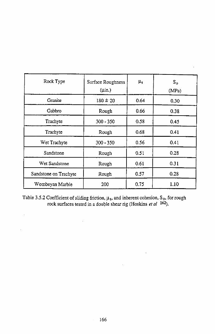
Rock Type Surface Roughness

()iin.)

Vs So

(MPa)

Granite 180 ± 20 0.64 0.30

Gabbro Rough 0.66 0.38

Trachyte 300 - 350 0.58 0.45

Trachyte Rough 0.68 0.41

Wet Trachyte 300 - 350 0.56 0.41

Sandstone Rough 0.51 0.28

Wet Sandstone Rough 0.61 0.31

Sandstone on Trachyte Rough 0.57 0.28

Wombeyan Marble 200 0.75 1.10

Table 3.5.2 Coefficient of sliding friction, fj.s, and inherent cohesion, S0, for rough rock surfaces tested in a double shear rig (Hoskins ei al 162).

166

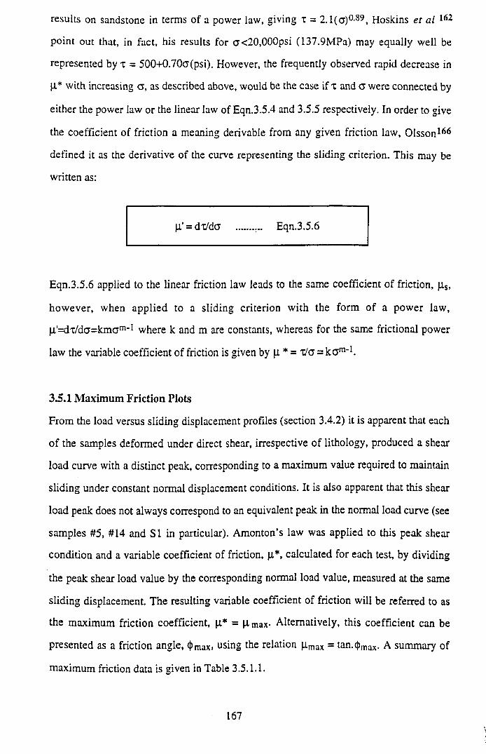
results on sandstone in terms of a power law, giving x = 2.1(a)0-89, Hoskins et al 162

point out that, in fact, his results for a<20,000psi (137.9MPa) may equally well be

represented by x = 500+0.70a(psi). However, the frequently observed rapid decrease in

|i* with increasing a , as described above, would be the case if x and a were connected by

either the power law or the linear law of Eqn.3.5.4 and 3.5.5 respectively. In order to give

the coefficient of friction a meaning derivable from any given friction law, Olsson166

defined it as the derivative of the curve representing the sliding criterion. This may be

written as:

p' = dx/da ........ Eqn.3.5.6

Eqn.3.5.6 applied to the linear friction law leads to the same coefficient of friction, p.s,

however, when applied to a sliding criterion with the form of a power law,

|i'=dx/da=km am’1 where k and m are constants, whereas for the same frictional power

law the variable coefficient of friction is given by (i * = x/cr = k a 1"’1.

3.5.1 M axim um Friction Plots

From the load versus sliding displacement profiles (section 3.4.2) it is apparent that each

o f the samples deformed under direct shear, irrespective of lithology, produced a shear

load curve with a distinct peak, corresponding to a maximum value required to maintain

sliding under constant normal displacement conditions. It is also apparent that this shear

load peak does not always correspond to an equivalent peak in the normal load curve (see

samples #5, #14 and SI in particular). Amonton’s law was applied to this peak shear

condition and a variable coefficient of friction, p.*, calculated for each test, by dividing

the peak shear load value by the corresponding normal load value, measured at the same

sliding displacement. The resulting variable coefficient of friction will be referred to as

the maximum friction coefficient, p* = Umax- Alternatively, this coefficient can be

presented as a friction angle, <t>max. using the relation p max = tan.<t>max. A summary of

maximum friction data is given in Table 3.5.1.1.

167

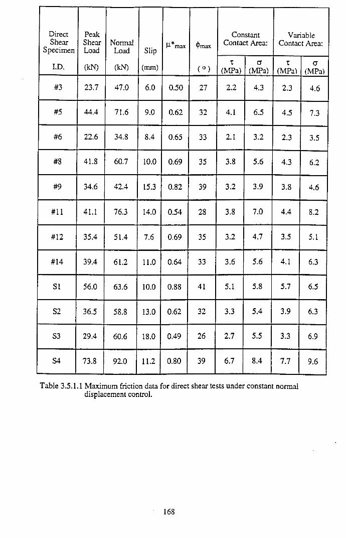
DirectShear

Specimen

PeakShearLoad

NormalLoad Slip

H*max 0maxConstant

Contact Area:Variable

Contact Area:

I.D. (kN) (kN) (mm) ( ° )X

(MPa)a

(MPa)X

(MPa)CT

(MPa)

#3 23.7 47.0 6.0 0.50 27 2.2 4.3 2.3 4.6

#5 44.4 71.6 9.0 0.62 32 4.1 6.5 4.5 7.3

#6 22.6 34.8 8.4 0.65 33 2.1 3.2 2.3 3.5

#8 41.8 60.7 10.0 0.69 35 3.8 5.6 4.3 6.2

#9 34.6 42.4 15.3 0.82 39 3.2 3.9 3.8 4.6

#11 41.1 76.3 14.0 0.54 28 3.8 7.0 4.4

oo

#12 35.4 51.4 7.6 0.69 35 3.2 4.7 3.5 5.1

#14 39.4 61.2 11.0 0.64 33 3.6 5.6 4.1 6.3

SI 56.0 63.6 10.0 0.88 41 5.1 5.8 5.7 6.5

S2 36.5 58.8 13.0 0.62 32 3.3 5.4 3.9 6.3

S3 29.4 60.6 18.0 0.49 26 2.7 5.5 3.3 6.9

S4 73.8 92.0 11.2 0.80 39 6.7 8.4 7.7 9.6

Table 3.5.1.1 Maximum friction data for direct shear tests under constant normal displacement control.

168

Following Byerlee13S, peak shear stress and corresponding normal stress (calculated

using both constant and slip-dependent variable contact areas) data is presented as

maximum friction plots in Fig.3.5.1.1. Byerlee’s relationship x = 0.85a (see Table 3.5.1)

representing the shear stress required to cause sliding under normal stresses up to

200MPa is also shown for the purposes of comparison. This relation was derived as a

linear best-fit to intermediate pressure (<100MPa) maximum friction data. At low normal

stresses (<5MPa) more in keeping with those generated during this direct shear study,

B yerlee’s maximum friction data, derived from a compilation o f published results

sourced from the civil engineering field, showed a wide scatter about x = 0.85a. This

large variation was interpreted as being due to the strong dependence of friction on

surface roughness at low normal stresses. From Fig.3.5.1.1, however, it is apparent that

the direct shear specimen maximum friction data plots consistently below Byerlee’s low

normal stress relation. This implies that the direct shear specimens were relatively weak

in comparison to the average from Byerlee’s compilation. Interestingly, the direct shear

maximum friction data would be better represented by Byerlee’s high normal stress

(200MPa<a<2000MPa) straight line relationship, x=0.5+0.6 a . This could reflect the

constant normal displacement shearing mode, and resultant total suppression of dilatancy,

under which all the direct shear tests were conducted. Byerlee’s low and high normal

stress linear friction laws doubtless reflect the different physical mechanisms involved in

the sliding process operative within these low and high pressure ranges. Specifically, at

low pressure the surfaces are free to move with respect to one another by lifting over

asperities, whilst at high pressure this effect is suppressed and sliding is achieved through

asperity shear. Perhaps the direct shear data fits the high pressure frictional relationship

more closely because the mechanism of asperity shearing is wholly dominant, even

although the normal stress magnitude never exceeds lOMPa? This would highlight an

important omission with regard to Byerlee’s interpretation, which fails to consider the

influence of discontinuity normal stiffness on the initial, maximum and residual friction.

Obviously the direct shear data set is at present too small to comment further. Fig.3.5.1.1

shows no evidence of clustering of data into specific lithological fields, in accord with

the observation of Byerlee that, “rock type has little or no effect on friction.”

169

o Peak

She

ar S

tress

(M

Pa)

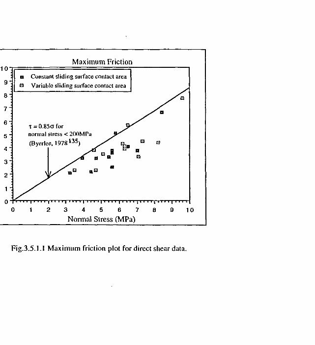
Maximum Friction

Fig.3.5.1.1 Maximum friction plot for direct shear data.

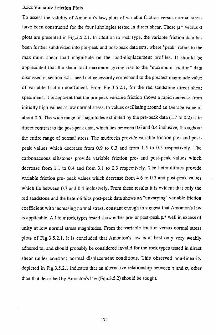
To assess the validity of Amonton's law, plots o f variable friction versus normal stress

have been constructed for the four lithologies tested in direct shear. These p.* versus a

plots are presented in Fig.3.5.2.1. In addition to rock type, the variable friction data has

been further subdivided into pre-peak and post-peak data sets, where "peak" refers to the

maximum shear load magnitude on the load-displacement profiles. It should be

appreciated that the shear load maximum giving rise to the "maximum friction" data

discussed in section 3.5.1 need not necessarily correspond to the greatest magnitude value

o f variable friction coefficient. From Fig.3.5.2.1, for the red sandstone direct shear

specimens, it is apparent that the pre-peak variable friction shows a rapid decrease from

initially high values at low normal stress, to values oscillating around an average value of

about 0.5. The wide range of magnitudes exhibited by the pre-peak data (1.7 to 0.2) is in

direct contrast to the post-peak data, which lies between 0.6 and 0.4 inclusive, throughout

the entire range of normal stress. The mudrocks provide variable friction pre- and post-

peak values which decrease from 0.9 to 0.3 and from 1.5 to 0.5 respectively. The

carbonaceous siltstones provide variable friction pre- and post-peak values which

decrease from 1.1 to 0.4 and from 3.1 to 0.3 respectively. The heterolithics provide

variable friction pre- peak values which decrease from 4.6 to 0.5 and post-peak values

which lie between 0.7 and 0.4 inclusively. From these results it is evident that only the

red sandstone and the heterolithics post-peak data shows an "unvarying" variable friction

coefficient with increasing normal stress, constant enough to suggest that Amonton's law

is applicable. All four rock types tested show either pre- or post-peak j i* well in excess of

unity at low normal stress magnitudes. From the variable friction versus normal stress

plots o f Fig.3.5.2.1, it is concluded that Amonton's law is at best only very weakly

adhered to, and should probably be considered invalid for the rock types tested in direct

shear under constant normal displacement conditions. This observed non-linearity

depicted in Fig.3.5.2.1 indicates that an alternative relationship between x and c , other

than that described by Amonton's law (Eqn.3.5.2) should be sought.

3.5.2 V ariable Friction Plots

171

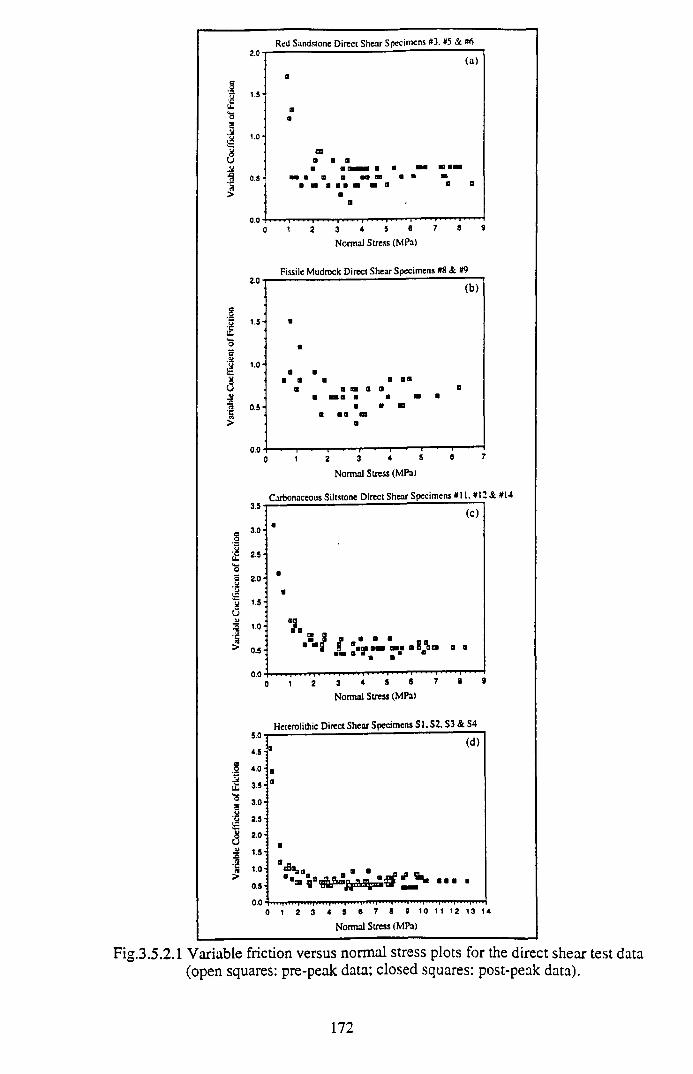
Red Sandstone Direct Shear Specimens #3. #5 & WS

Fissile Mudrock Direct Shear Specimens #8 & #9

Carbonaceous Siltstone Direct Shear Specimens #11. #12 & #14

Heterolithic Direct Shear Specimens S I. S2. S3 & S4

Normal Stress (MPa)

Fig.3.5.2.1 Variable friction versus normal stress plots for the direct shear test data (open squares: pre-peak data; closed squares: post-peak data).

172

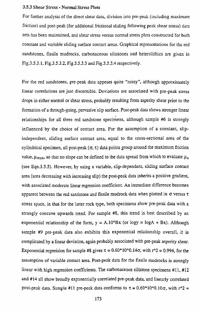
3.5.3 Shear Stress - Normal Stress Plots

For further analysis of the direct shear data, division into pre-peak (including maximum

friction) and post-peak (for additional frictional sliding following peak shear stress) data

sets has been maintained, and shear stress versus normal stress plots constructed for both

constant and variable sliding surface contact areas. Graphical representations for the red

sandstones, fissile mudrocks, carbonaceous siltstones and heterolithics are given in

Fig.3.5.3.1, Fig.3.5.3.2, Fig.3.5.3.3 and Fig.3.5.3.4 respectively.

For the red sandstones, pre-peak data appears quite “noisy”, although approximately

linear correlations are just discernible. Deviations are associated with pre-peak stress

drops in either normal or shear stress, probably resulting from asperity shear prior to the

formation of a through-going, pervasive slip surface. Post-peak data shows stronger linear

relationships for all three red sandstone specimens, although sample # 6 is strongly

influenced by the choice of contact area. For the assumption of a constant, slip-

independent, sliding surface contact area, equal to the cross-sectional area of the

cylindrical specimen, all post-peak (O’, t) data points group around the maximum friction

value, | i max. so that no slope can be defined to the data spread from which to evaluate [is

(see Eqn.3.5.5). However, by using a variable, slip-dependent, sliding surface contact

area (area decreasing with increasing slip) the post-peak data inherits a positive gradient,

with associated moderate linear regression coefficient. An immediate difference becomes

apparent between the red sandstone and fissile mudrock data when plotted in a versus x

stress space, in that for the latter rock type, both specimens show pre-peak data with a

strongly concave upwards trend. For sample #8 , this trend is best described by an

exponential relationship of the form, y = A.10ABx (or logy = logA + Bx). Although

sample #9 pre-peak data also exhibits this exponential relationship overall, it is

complicated by a linear deviation, again probably associated with pre-peak asperity shear.

Exponential regression for sample #8 gives x = 0.60* 10A0.14a, with rA2 = 0.994, for the

assumption of variable contact area. Post-peak data for the fissile mudrocks is strongly

linear with high regression coefficients. The carbonaceous siltstone specimens #11, #12

and #14 all show broadly exponentially correlated pre-peak data, and linearly correlated

post-peak data. Sample #11 pre-peak data conforms to t = 0.69* 10A0.10<r, with rA2 =

173

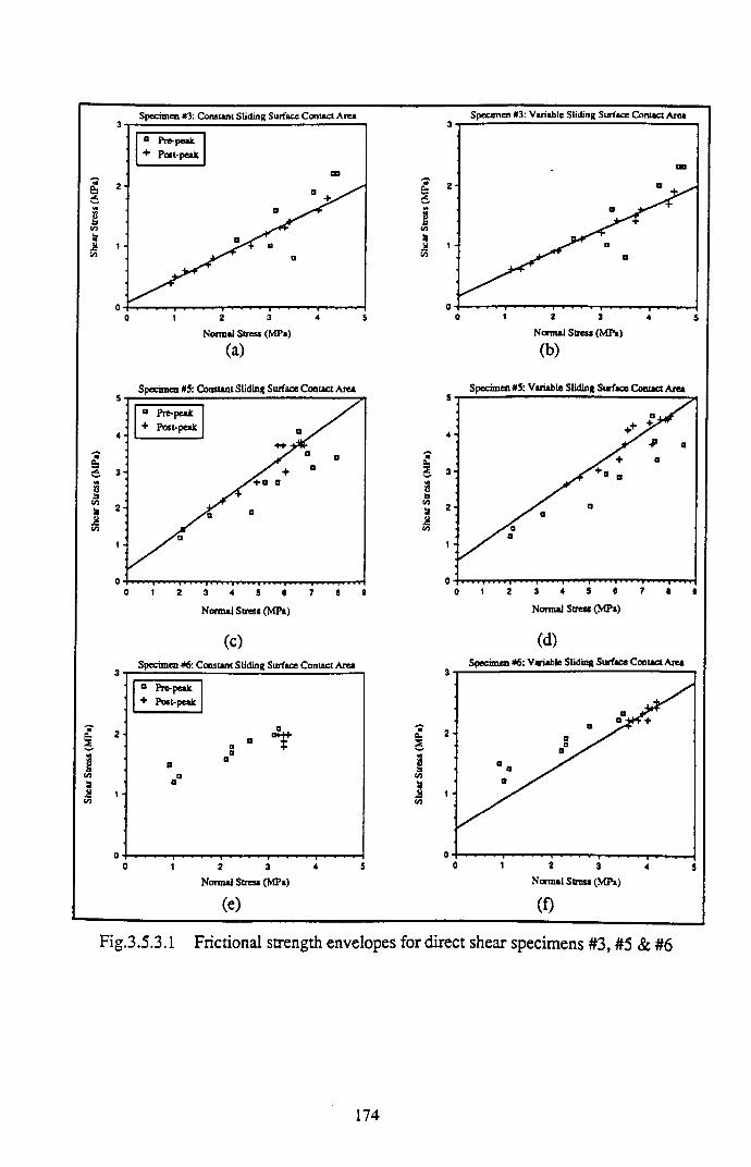
Shea

r Stre

ss (M

Pa)

Shea

r Stre

ss (M

Pa)

(a)

Specimen #3: Variable Sliding Surface Contact Area

(b)

Fig.3.5.3. 1 Frictional strength envelopes for direct shear specimens #3, #5 & # 6

174

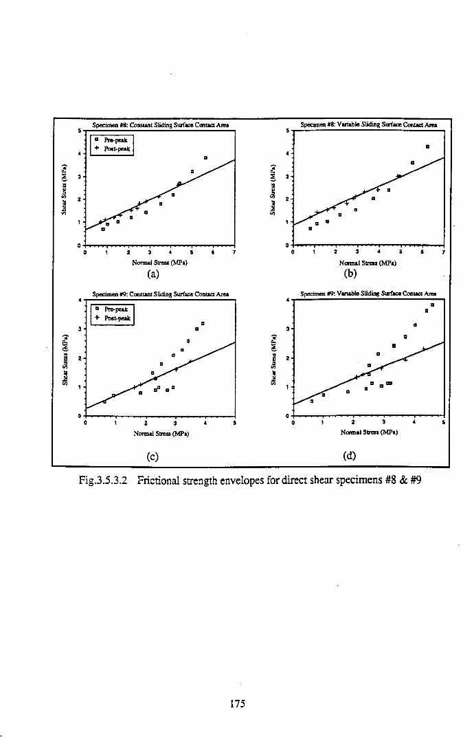
(a) (b)

Specimen #9: Constant Sliding Surface Contact Area Specimen #9: Variable Sliding Surface Contact Area

(C) (d)

Fig.3.5.3.2 Frictional strength envelopes for direct shear specimens # 8 & #9

175

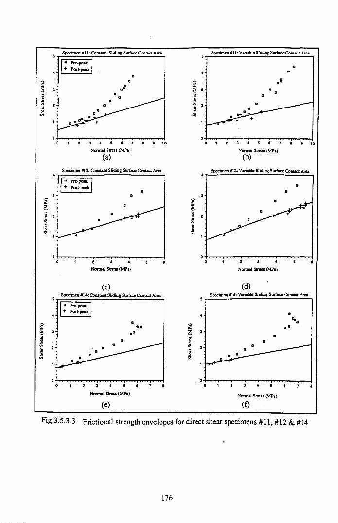
(a)Specimen #12: Constine Sliding Surface Contact Area

(c)

(e)

(b)

Specimen #12: Variable Sliding Surface Contact Area

(d)

(f)Fig.3.5.3.3 Frictional strength envelopes for direct shear specimens #11, #12 & #14

176

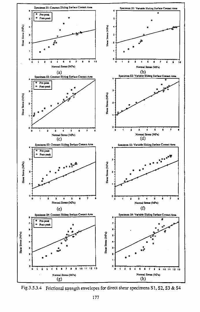
Shea

r Stre

ss (M

Pa)

Shea

r Stre

ss (M

Pa)

Shea

r Stre

ss (M

Pa)

Specimen SI : Constant Sliding Surface Contact Area

£cnh

(a)Specimen S2: Constant Sliding Surface C onua Area

(C)Specimen S3: Constant Sliding Surface C onua Area

(e)

Normal Stress (MPa)

(g)

(b)Specimen S2: Variable Sliding Surface Contact Area

(d)Specimen S3: Variable Sliding Surface C onua Area

(f)Specimen S4: Variable Sliding Surface C onua Area

(h)Fig.3.5.3.4 Frictional strength envelopes for direct shear specimens S I, S2, S3 & S4

177

0.995, for the assumption of variable contact area. The heterolithic specimens, with the

exception o f sample S3, all show broadly exponentially correlated pre-peak data, and

linearly correlated post-peak data. Sample SI pre-peak data has the form t =

0.56* 10A0.16a, with rA2 = 0.975, for the assumption of variable contact area. However,

sample S3 shows a strong concave downwards trend between increasing a and x

inconsistent with an exponential relationship. Instead, it is best represented by a

logarithmic relationship of the form, y = A + Blogx, with X = 1.06 + 2.45*loga, rA2 =

0.978, for the assumption of variable contact area. This pre-peak data logarithmic

relationship might reflect relative rotation between upper and lower specimen halves.

Post-peak data for SI is, however, still linear, with a regression coefficient of 1.00. In

fact, independent o f rock type, all specimens tested in direct shear under constant normal

displacement conditions, showed linear relationships between a and x for frictional

sliding subsequent to the attainment of maximum friction conditions.

Tabulated values of frictional sliding constants |TS (slopes) and S 0 (intercepts) are given in

Table 3.5.3.1. The slopes and intercepts were calculated for “best fit” straight lines,

determined using linear regression analysis based on the principle of least squares, as

outlined in Barford (1987)168 together with standard errors for each slope and intercept,

Sn(p.s) and Sn(S0) respectively. From Table 3.5.3.1 it is apparent that the choice of either

a constant or a variable sliding surface contact area has a marked effect on the magnitude

of the frictional sliding constants, (is and S0. With regard to friction angles, <J>S (where 0 S

= tan^jis) this is evident in up to 7° difference between calculated constants. However,

this difference resulting from whether a constant or a variable contact area is chosen, is

small compared with the difference between maximum friction angles, bmax. (see Table

3 .5 .1.1) and sliding friction angles, <j>s. which can be in excess of 30° (specimen SI).

Inherent shear strength, S0, of the post-peak sliding surfaces, was also found to be

moderately dependent on the choice of a constant or a variable contact area. Magnitudes

ranged from a few tenths of a MPa (specimen #3) to over 2MPa (specimen S4). Finally,

in accord with the observation made for maximum friction, no obvious correlation was

evident between rock type and the magnitude of either of the post-peak frictional sliding

constants, |i s o rS 0.

178

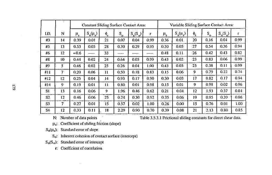
ID . N

Constant Sliding Surface Contact Area: Variable Sliding Surface Contact Area:

V* W So W r *ls SA ) So s (S )nv cr r

#3 14 0.39 0.01 21 0.07 0.04 0.99 0.36 0.01 20 0.16 0.04 0.99

#5 13 0.53 0.05 28 0.30 0.29 0.95 0.50 0.05 27 0.54 0.36 0.94

#6 12 « 0 .6 — 33 0.48 0.11 26 0.42 0.43 0.82

#8 10 0.44 0 .0 2 24 0.64 0.05 0.99 0.43 0 .0 2 23 0.83 0.06 0.99

#9 5 0.46 0 .02 25 0.26 0.04 1.00 0.43 0.03 23 0.38 0.11 0.99

#11 7 0 .2 0 0.06 11 0.50 0.18 0.83 0.15 0.06 9 0.79 0 .22 0.74

#12 12 0.25 0.04 14 0.93 0.17 0.90 0.30 0.03 17 0.82 0.17 0.94

#14 9 0.19 0.01 11 0.80 0.01 0.98 0.15 0.01 9 0.98 0 .02 0.96

SI 13 0.16 0.06 9 1.96 0.46 0.62 0.21 0.04 12 1.93 0.37 0.84

S2 12 0.46 0.06 25 0.24 0.30 0.92 0.35 0.06 19 0.95 0.39 0 .86

S3 7 0.27 0.01 15 0.57 0 .02 1.00 0.26 0 .0 0 15 0.76 0.01 1.00

S4 12 0.33 0.11 . 18 2.29 0.90 0.70 0.39 0.08 21 2.13 0.80 0.85

N: Number of data points Table 3.5.3.1 Frictional sliding constants for direct shear data.|i s: Coefficient of sliding friction (slope)

S„(Hs): Standard error of slope

SQ: Inherent cohesion of contact surface (intercept)

Sn(S0): Standard error of intercept n Coefficient of correlation

3.6 DISCUSSION

From the above considerations of shear stress versus normal stress relations and frictional

strength criteria, with respect to slip in direct shear under constant normal displacement

conditions, it is evident that the frictional sliding mechanism can be envisaged as a two-

stage process. Initially, for sliding displacements up to and including that associated with

peak shear stress (maximum friction) conditions, such pre-peak data shows exponential

increase in x with increasing a for the majority of samples tested. Exceptions include the

red sandstone specimens which show poorly correlated linear a versus x relationships,

indicative perhaps of an incipient lithological dependency. Heterolithic specimen S3

exhibits a logarithmic relationship between pre-peak (t, c ) data, which may reflect

relative rotation between the upper and lower sample halves. Pre-peak data is further

complicated by linear deviations from the gross o versus x relationship, associated with

pre-peak stress drops in the shear and normal stress versus sliding displacement profiles,

resulting from localised asperity shear. Fissile mudrock specimen #9 illustrates this

phenomenon particularly clearly, where a stress drop primarily in the normal stress versus

sliding displacement profile has resulted in a prominent linear deviation from the overall

exponentially correlated pre-peak data. In direct contrast to the pre-peak data discussed

above, post-peak (x, o ) points define robust straight line relationships for all twelve

specimens tested in the constant normal displacement shearing mode. In physical terms,

the maximum friction point is thus interpreted as representing peak shear strength of the

sliding discontinuity, immediately prior to pervasive breaching of the interlocking

asperity system (usually associated with a significant, and frequently audible dynamic

stress drop as illustrated by specimens #5, #8 , #9, #11, #12, #14, S I, S2, S3 & S4)

followed by frictional sliding on the newly created and pervasive shear plane. Post­

mortem examination reveals this plane to be composed of frictionally comminuted shear

debris (analogous to natural fault gouge) which frequently shows steps and slip-parallel

striae (analogous to slickensides and related features as observed on natural fault

surfaces). Thus true “residual” strength when shearing under constant normal

displacement conditions is perhaps best described by the constants jis and S 0 as defined in

Eqn.3.5.5.

180

Corroboration of the above experimental observations relating to the development of

shear strength for a frictional discontinuity undergoing constant normal displacement

shearing, can be found in Gerrard (1986)169. By the application of appropriate theoretical

constraints pertaining to “shear failure” of rock discontinuities, Gerrard was able to assess

various empirical relations and to develop formulations for strength and dilatancy. In his

analysis, the rock discontinuity was imagined as consisting of an array of contacts, as a

means of establishing a basis for mechanical properties determination, its shear strength

being inferred to consist of both “fracture” and “friction” components. At these contacts

deformation was considered to occur by a combination of elastic, crushing, sliding and

ploughing processes. In general, during shear failure of a rock discontinuity, all of these

processes were considered to be operative, with sliding and ploughing being dominant.

Due to the range of contact orientations, Gerrard proposed that their shear behaviour

ranged from sliding to heavy ploughing, the shear strength of each contact thus being

envisaged as consisting of a component required for “fracturing” and a component

required for “sliding” (usually inclined to the plane of the discontinuity). Through

summation, these shear strength components for an individual contact would be reflected

in the corresponding components for the rock discontinuity as a whole, as expressed in

Gerrard’s following general failure criterion:

F = 0 = (x - a - ciii)/Gr .......... Eqn.3.6.1

F: failure criterion

x, g : shear and normal stresses

Gr: reference stress

a: component of shear strength due to fracturing

JJ-i: effective coefficient of friction for inclined sliding

Jaeger & Cook8 showed that the effective coefficient of friction for inclined sliding is

given by:

181

Pi = (P + g ) /( l- |ig ) .......... Eqn.3.6.2

fj,¡ = tanc{>¡ = tan(<}) V|/) .......... Eqn.3.6.3

p: effective coefficient of friction for sliding without dilation = tan<|>

g: gradient of the dilation at failure = tanvj/

Gerrard proposed that the factors affecting the shear strength of a rock discontinuity can

be identified by considering the terms involved in Eqn.3.6.1, Eqn.3.6.2 and Eqn.3.6.3.

The component of shear strength due to fracturing alone, a, will depend on the hardness

and toughness of the asperities and on their average height and radius. It will also depend

on the normal stress and will tend to zero as a —» 0. The effective coefficient of friction

for sliding without dilation, )i, will vary between two extreme conditions. One of these

will be the case of minimal damage of the asperities, this being applicable to the case

when the normal stress, a, is relatively low and the asperities have enhanced strength due

to the combined effects of favourable surface topography and hardness/toughness. The

appropriate coefficient of friction for this condition will be that for sliding of smooth

surfaces of the rock material, p smooth- The other extreme will occur when extensive

fracturing of the asperities is induced during shear failure of the rock discontinuity. This

condition is associated with relatively high normal stress and/or relatively weak asperities

due to unfavourable surface topography and hardness/toughness. It appears that two

coefficients of friction are relevant. The first, {ipeak. relates to the process o f actually

creating the fractures through the asperities, while the second, p residual, relates to the

sliding over the resultant freshly fractured surfaces and debris. For this condition of

extensive fracturing, jipeak will be associated with peak strength whilst Presidual will be

associated with the residual strength. Gerrard’s analysis assumes that, for a given rock

discontinuity, | iSmooth> Ppeak, and p.residual can have different values. Thus there appears

to be a direct analogy between Gerrard’s peak and residual coefficients, Ppeak an<i

Presidual for sliding without dilatancy, and the empirically derived frictional coefficients,

Umax and | i s respectively, tabulated from this direct shear experimental study.

182

4. COUPLED PERM EABILITY-M ICROSEISM ICS M EASUREM ENT DURING

TRIAXIAL COMPRESSION TESTING: EQUIPM ENT DEVELOPM ENT

4.1 INTRODUCTION

In a review of the various laboratory apparatus used for shear testing of rock

discontinuities (see summary Table 4.1.1) the important point is made that each possesses

distinct experimental advantages, as well as certain limitations, necessitating careful

matching of experimental requirements with equipment strengths. Whilst the direct shear

machine allows testing of relatively large shear surface areas under known boundary

conditions, ideal for fundamental frictional strength studies, to investigate the effects of

faulting on fluid flow under realistic reservoir stress magnitudes, the discontinuity triaxial

compression test is better suited, due to technical difficulties involved in confining direct

shear specimens, and in adequately sealing the sliding interface for fluid flow studies. In

contrast, the triaxial method offers a facility for breaking cylindrical rock specimens in

shear under differential axial and radial stresses, whilst simultaneously monitoring (albeit

discontinuously) transient core plug permeability allied with changing stress states

ranging from hydrostatic to those operative during post-peak frictional sliding conditions.

The limitations of the triaxial test system are that: only axial stress and confining pressure

( c i and 0 3 ) as opposed to shear and normal stresses are directly controllable; geometric

constraints make only very small sliding displacements (of the order of a couple of mm's

maximum) achievable; induced fault orientation is oblique to the specimen long axis and

thus oblique to the direction of fluid flow associated with permeability measurement.

The system used to investigate laboratory induced faulting in core specimens essentially

consists of three individual components, stress application, permeability measurement

and microseismic monitoring. This system, and the interconnection of its individual

components, is illustrated schematically in Fig.4.1.1. Each core plug is subjected to

realistic in situ reservoir stress magnitudes, and ultimately to differential stresses

resulting in shear failure, using a 100T stiff servo-hydraulic compression rig and

"Hoek/Franklin-type" 10 OOOpsi-rated confining pressure cell combination (the triaxial

183

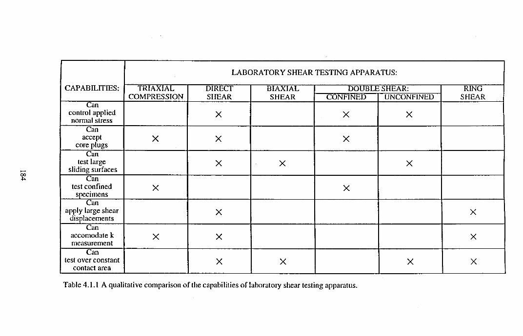
CAPABILITIES:

LABORATORY SHEAR TESTING APPARATUS:

TRIAXIALCOMPRESSION

DIRECTSHEAR

BIAXIALSHEAR

DOUBLE SHEAR: RINGSHEARCONFINED UNCONFINED

Cancontrol applied normal stress

X X X

Can accept

core plugsX X X

Cantest large

sliding surfacesX X X

Cantest confined

specimensX X

Canapply large shear

displacementsX X

Canaccomodate k measurement

X X X

Cantest over constant

contact areaX X X X

Table 4.1.1 A qualitative comparison of the capabilities of laboratory shear testing apparatus.

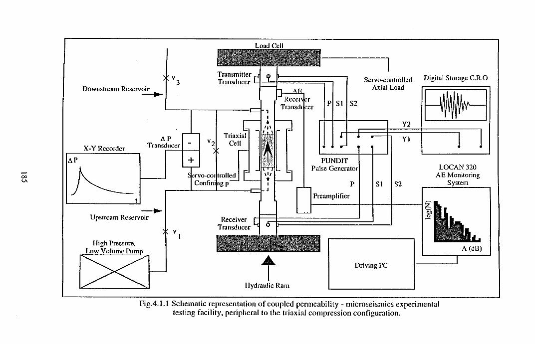
Fig.4.1.1 Schematic representation o f coupled permeability - microseismics experimental testing facility, peripheral to the triaxial compression configuration.

compression setup). This system forms the "backbone’’ of the rock mechanics research

facility. Envisaging the "in situ" rockmass as an anisotropic and heterogeneous

assemblage of intact/microcracked rock elements separated by planar discontinuities

(joints, faults and bedding planes) the triaxial setup enables the deformability, strength

and fluid flow characteristics o f core plugs (representing intact blocks) to be

characterised, complementing discontinuity deformability and strength parameters as

measured using the direct shear rig. By such means, important constitutive stress-strain

relations and permeability data is generated which can be incorporated directly into

numerical reservoir simulation. Whilst fault sealing is currently assessed using the triaxial

compression method to induce shear fracturing, it is however hoped that further

equipm ent development will allow the perm eability/transmissibility of frictional

interfaces tested under direct shear conditions to be achieved.

Linked to the triaxial compression system is a coupled permeability-microseismic facility

which allows measured changes in pemeability resulting from controlled variation in the

applied triaxial stress field, to be related to microstructural deformation processes

occurring within the core specimen (including elastic pore closure, inelastic grain­

boundary sliding, axial microcracking etc). The permeameter system basically comprises

a high pressure low volume pump, differential pressure transducer, x-y-t plotter assembly,

enabling either steady-state or transient pulse-decay absolute liquid permeability

measurements to be conducted using a variety of pore fluids including refined mineral

oils, distilled water, brines and artificial seawaters of varying composition. The

microseismics system incorporates both passive (acoustic emission, AE) monitoring and

active (artificial compressional- and orthogonally polarised shear-wave) techniques. In

Fig.4.1.1 the active transmitting and receiving transducers are shown mounted

respectively above and below the rock specimen loading platens, whilst the AE

transducer is shown mounted on the end of a waveguide which pierces the body of the

confining pressure cell. For this present study only passive AE monitoring was conducted

to assess microstructural evolution. Both the permeability and microseismic systems are

mounted on separate trolleys for manoeuvrability, so that they can be positioned by the

compression rig when required, as shown in Fig.4.1.2.

186

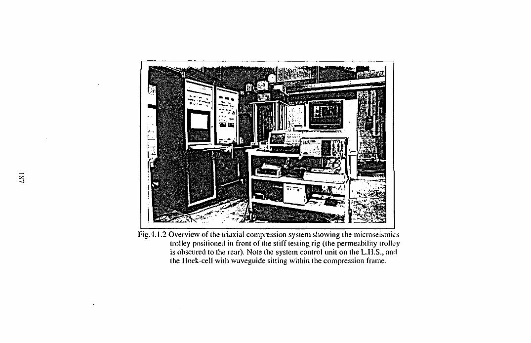
Fig.4.1.2 Overview of the triaxial compression system showing the microseismics trolley positioned in front of the stiff testing rig (the permeability trolley is obscured to the rear). Note the system control unit on the L.I1.S., and the Hoek-cell with waveguide sitting within the compression frame.

In the following chapter, details of the triaxial compression system, and of the coupled

permeability-microseismics facility are outlined. Information on the stiff compression rig

was obtained primarily from the RDP-Howden Customer Instruction and Maintenance

Manual (1984)170. Specifics relating to the pulse-decay permeability technique were

found from McMeekin (1991)171 and Smart et al (1992)172. Acoustic emission system

description and operating procedures were sourced from the LOCAN-320 User’s Manual

(1988) l72. Also, as a useful additional reference dealing with general instrumentation and

control theory, Haslam et al (1991)174 proved invaluable.

4.2 STRESS A PPLICATION

The simplest and most commonly used procedure for achieving a triaxial state of stress in a

laboratory test is to superimpose a hydrostatic pressure and a uniaxial stress. Such a test is

usually referred to simply as a “triaxial test” following the nomenclature of soil mechanics

(of course the test is only a special case of triaxial stress in which the intermediate principal

stress is always equal to one or other of the extreme principal stresses, but the term is

widely used without qualification to refer to these conditions). Since, in these tests,

cylindrical specimens are subjected to simple compression or extension in the presence of a

superposed hydrostatic pressure, the state of stress in the specimen ideally consists of two

equal principal stresses normal to the compression or extension axis and a third principal

stress parallel to it. Adopting the convention common in geologic and rock mechanics

literature that compressive stress is positive, and designating the greatest, intermediate and

least principal stresses c i , <3 2 and a 3 respectively, the applied stress in a triaxial

compression test is as shown in Fig.4.2.1. The two equal stresses have the same magnitude

as the superposed hydrostatic pressure, whilst the third principal stress departs from it. The

superposed hydrostatic pressure is called the confining pressure since it is the pressure in

the m edium surrounding the specimen (note that this is not the same as the

mean/nondeviatoric stress in the specimen, which is equal to l/3 (a i + 2 (J3) in the triaxial

compression test). The amount by which the axial stress departs from the confining

pressure is called the differential stress and is commonly designated by gj - C3.

188

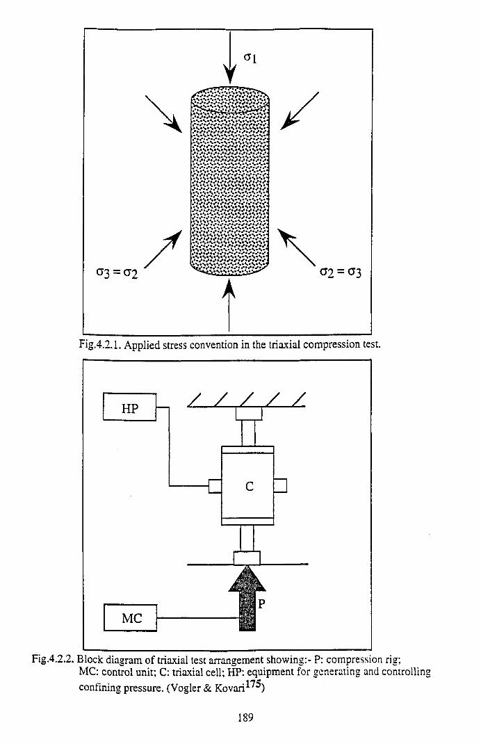
y<*i

(T3 = C2

■* l ì i i j i ‘ ~ ■“ ■ ■ ' ■ i , i ■ f i r■ S ■ S • % % ■ N ■ e• s »s «s «* »* s »s »s * s »s »s * *

• • S 'S 'S 'S 'S 'S ^ S ^ S i S 'N * ' i » \ » S » V S » % * S * S 'S * S * V < i » S * S » S » V » N * S » S * S * S * % * 1

• S " S »S * S »S «S »S «S »S «S »*• s ■ % •% * S -S «S • ‘s » s - s ■ % ■■■ S . S . S . S . S « <•V •“« *7 **; «V «*; •*: w*.• S»S aS*%*S*%*S*S*SaS »4«■; **■ «*; «*; ** ■ «’• •*; «*■

• S iS * S iS .M S .S * S .% > S « <

, i S i S i *i i S i S > S * % « S > S * S i <,> \*% iS iS iS «S *S *S *% *S ia/ • / ; /■ «*; •*.■ •* ; ■ V ; •*;• S*S«S*SaN aS aS«Sa*a*S*a.■ S " S »S * S «N «S " S «S aS »S * a• S > S < S 'S * S iN * S a S * % « S * a• S . i . .M S i S > S * S * S * % * S Vï s V s V % . s - s - s . \ - s . s - s - - • s « s » s * s » s » % » s » s » s » s « a • N « S » S » S * S » S * S , N , S , S ê‘ V s V ^ .S «N -S * S «S * S »% * S * ‘3 ^ - < 1 S » s » S ■ Ñ «S "S

A

/

\<Ï2 = ° 3

Fig.4.2.1. Applied stress convention in the triaxial compression test.

Fig.4.2.2. Block diagram of triaxial test arrangement showing:- P: compression rig;MC; control unit; C: triaxial cell; HP: equipment for generating and controllingconfining pressure. (Vogler & K o v a r i^ )

189

For the application of nonhydrostatic triaxial stress states, the ability to apply an axial stress

to the specimen independent of the radial confining pressure is fundamental. In such

conventional triaxial testing of core plugs, a uniform radial stress is usually applied

hydraulically to the curved surface of the rock cylinder, whilst simultaneously the prepared

flat and parallel specimen ends are loaded axially through spherical seats and platens. In

terms of equipment used, radial pressurisation or confinement is usually achieved through a

pressure vessel in which hydraulic fluid at pressure, p, acts on a synthetic rubber

membrane sheathing the sample. Axial load is generated parallel to the specimen long axis

via a stiff, servo-hydraulic compression machine. In this manner, axial loading over the

specimen cross-sectional area results in an axial stress, <7a, wholly independent of p. Two

admissible stress field conditions are thus within the limitations of conventional triaxiai

testing, resulting from independent control of a a and p:

(i) triaxial compression, where c a = C7i > C2 = 03 = P

(ii) triaxial extension, in which a 1 = 02 = p >

Thus apparatus for achieving triaxial stress states on cylindrical rock specimens,

essentially consists of three components as indicated schematically in Fig.4.2.2: a loading

device for applying, controlling and measuring axial load, a triaxial cell for applying

confining pressure to the curved specimen surface, and equipment for generating and

measuring the confining pressure (Vogler & Kovari, 197717S).

Before the peak of the load-deformation curve is reached, work must always be done on

the combined specimen-machine system in bringing about an increment of deformation in

the specimen. The system is therefore, in this case, inherently stable mechanically.

However, beyond the peak, because potential energy is released from the machine as the

load decreases, it is possible that the work needed for further deformation of the specimen

can be fully provided from within the specimen-machine system, so that the deformation

process can continue spontaneously and uncontrollably, preventing the load-bearing

capacity of the specimen from being readily assessed as a function of the deformation,

and leading rapidly to destruction of the specimen. This situation is normal with the

190

brittle failure of a rock specimen in a conventional “soft” testing machine, especially a

machine with hydraulic loading. This problem is comprehensively discussed in rock

mechanics textbooks and will not be further reviewed here (for a more detailed discussion

see: Paterson, 19789, p.138-141; Jaeger and Cook, 1979s, p.177-183; Goodman95, p.76-

78). To study the complete progression of the failure process beyond peak load, two

experimental approaches have been made to overcome the limitation just described. One

is to use a “s tif f ’ testing machine, and the other to use a suitably servo-controlled

machine. With regard to the former approach, the complete load-deformation curve can

be followed at will if the stiffness of the machine corresponds to a slope that is steeper

than the most steeply descending part of the load-displacement curve of the specimen.

The most obvious step is therefore to use a machine of massive construction, although

loading of elastic elements in parallel with the specimen, and use of mercury as a

hydraulic fluid have also been tried. With respect to the latter experimental approach, in

the servo-control of a testing machine for post-failure studies, positive steps are taken to

unload the specimen when less load is required for its further deformation, without

relying on the stiffness of the machine. Normally the load control is achieved by

programming the machine to follow a prescribed displacement sequence, so that if the

displacement at the specimen begins to run ahead of the prescribed course, the servo-

control reduces the load being applied by the machine, usually by extracting oil from the

loading ram.

The mainstay o f the stress application apparatus for achieving triaxial loading of

cylindrical rock specimens, is a stiff (>2500 kN/mm) servo-hydraulic compression rig for

applying axial loads up to lOOOkN over the prepared flat and parallel core plug ends. The

compression machine comprises a four column fixed crosshead straining frame

incorporating a double acting unequal area actuator with integral displacement

transducer. Specimens are tested between this piston rod and a strain gauged load cell

attached to the fixed crosshead. The basics of the compression rig’s servo-control system

are described below. Closed-loop control of a conventional hydraulic system is achieved

by obtaining an electrical feedback signal, Vf, from a transducer tightly coupled to the

mechanical parameter to be controlled, e.g. load displacement or strain. This signal is

191

compared with the command signal, VC) and the error signal, Ve=Vc-Vf, is amplified to

drive the mechanical system to the commanded condition. The principles of operation of

a basic closed loop electro-hydraulic servo system are outlined in Fig.4.2.3. The

following numbers in square brackets refer to specific components as illustrated.

Pressurised oil from a hydraulic power pack [1] is fed via an electro-hydraulic servovalve

[2] to a double acting linear actuator [3] causing movement of the piston resulting in the

specimen [4] being loaded. Load, displacement and strain transducers [5, 6 & 7] may be

used in the system with their respective amplifiers [8, 9 & 10] producing voltage signals

proportional to the individual parameters. These are connected via a control console [11]

to the servo-amplifier [12]. This unit compares the “command” from a signal generator

[13] with the selected control parameter and drives the servovalve with the amplified

error signal. This results in any difference between the “command” and “actual” signals

being corrected.

Radial specimen confinement is achieved using a confining pressure intensifier and

pressure vessel system. The pressure intensifier is a high response servo-hydraulic unit

for controlling the confining pressure of the triaxial cell. The intensifier operates at

pressures up to 1 lOMPa over an 80cc volume change from a 30MPa external hydraulic

power supply (also supplying the compression and direct shear rigs) controlled by an

electro-hydraulic servovalve operating under closed loop control with pressure or volume

as the feedback parameter. A strain gauged pressure transducer measures the output

pressure whilst an internal transducer senses the change in volume over the entire

operating range. Volume change measurement is accomplished by a displacement

transducer connected to the intensifier piston. The triaxial cell used in this study was of a

design known as the “Hoek-type”, named after one of the inventors (Hoek and Franklin,

1968176; Franklin and Hoek, 1970177) and comprises: a cell body into which the

specimen may be placed in order to apply the confining pressure, this body having an air

bleeder-hole and a connection for a hydraulic line; threaded end-caps for ease of

deformed specimen removal from the cell; a flexible jacket (usually synthetic rubber) to

prevent the hydraulic fluid from entering the specimen. The Hoek-cell is rated to a

maximum operating pressure of 10 OOOpsi (68.9MPa) and was of a size suitable for 1.5"-

192

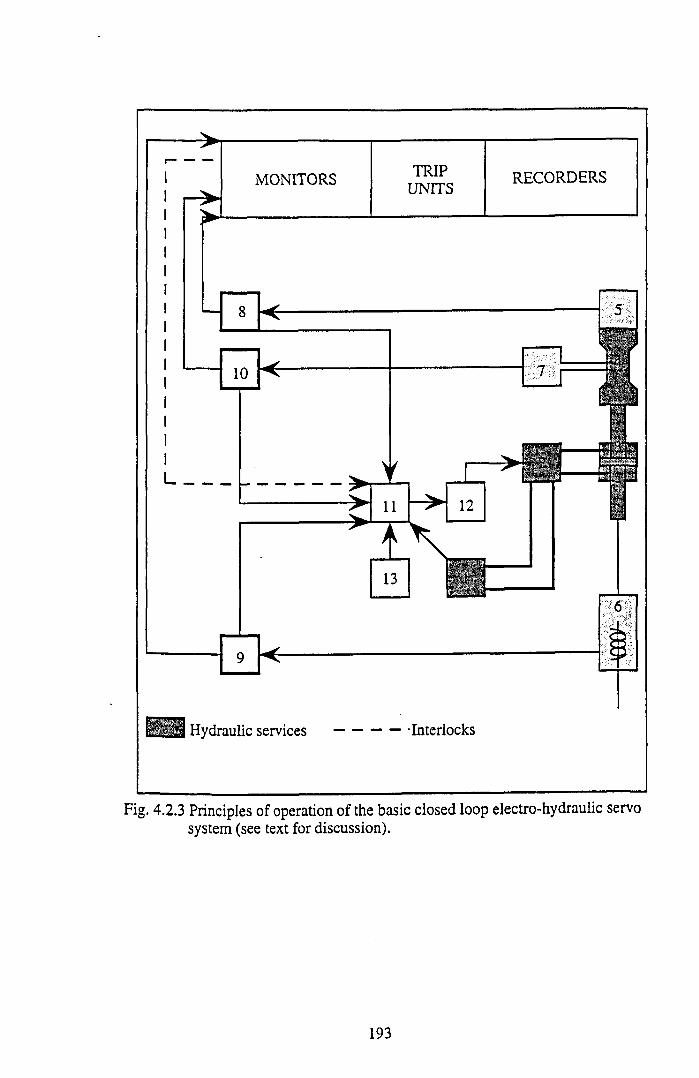
fcrXvjd Hydraulic s e r v i c e s ------------- -Interlocks

Fig. 4.2.3 Principles of operation of the basic closed loop electro-hydraulic servo system (see text for discussion).

193

(38.1m m -) d iam eter specim ens. For coupled perm eab ility -m icroseism ics

experimentation, the body of the standard Hoek-type triaxial cell as described above, has

been modified to accept a waveguide, in order to facilitate optimum coupling between the

acoustic emission sensor and the stressed rock sample. ISRM recommended procedures

for triaxial compression testing, which discuss equipment specifications, can be found in

Vogler and Kovari17S.

4 J PERM EABILITY MEASUREMENT

Permeability measurements are some of the most essential performed on core plugs from

recovered reservoir whole core. They represent important input data for accurate reservoir

characterisation and reserves estimation, and aid in the selection of recovery processes.

However, routine plug permeabilities are normally measured at lower stress magnitudes

than those operative in the reservoir environment, and further, the applied laboratory

stress field is invariably hydrostatic. Given the complex nature of the in situ rock stress

field, and the relative sensitivity of measured plug permeability to the laboratory applied

stresses, routine core analysis data should be treated with caution. Holt (1990)1878

provides both a summary of previous stress-dependent permeability measurements

conducted under hydrostatic conditions, and presents permeability reduction data induced

by non-hydrostatic stress fields.

4.3.1 The Pulse-Decay Permeability M ethod

W hilst previous studies of permeability sensitivity to applied stress, utilising the

permeameter system components described below, made use of steady state conditions to

evaluate changing fluid flow potential, for this experimental programme in which test

specimens will be subjected to high differential stresses resulting ultimately in post-peak

dynamic instability and macroscopic shear failure, a “pseudo-pulse decay” method was

preferentially employed in recognition thatlow permeability magnitudes would be

encountered in cores subjected to high differential stress states and that large quantities of

fines would be generated by frictional sliding

194

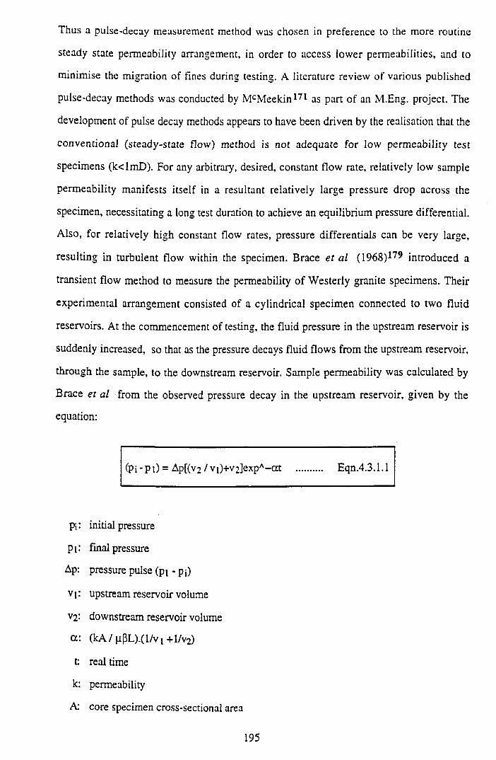
Thus a pulse-decay measurement method was chosen in preference to the more routine

steady state permeability arrangement, in order to access lower permeabilities, and to

minimise the migration of fines during testing. A literature review of various published

pulse-decay methods was conducted by McM eekin171 as part of an M.Eng. project. The

development of pulse decay methods appears to have been driven by the realisation that the

conventional (steady-state flow) method is not adequate for low permeability test

specimens (k<lmD). For any arbitrary, desired, constant flow rate, relatively low sample

permeability manifests itself in a resultant relatively large pressure drop across the

specimen, necessitating a long test duration to achieve an equilibrium pressure differential.

Also, for relatively high constant flow rates, pressure differentials can be very large,

resulting in turbulent flow within the specimen. Brace et al (1968)17^ introduced a

transient flow method to measure the permeability of Westerly granite specimens. Their

experimental arrangement consisted of a cylindrical specimen connected to two fluid

reservoirs. At the commencement of testing, the fluid pressure in the upstream reservoir is

suddenly increased, so that as the pressure decays fluid flows from the upstream reservoir,

through the sample, to the downstream reservoir. Sample permeability was calculated by

Brace et al from the observed pressure decay in the upstream reservoir, given by the

equation:

(Pi - P l) = Ap[(v2 / v 1) + V 2 ] e x p A- c c t .......... Eqn.4.3.1.1

pi: initial pressure

Pi: final pressure

Ap: pressure pulse (pi - pO

v i: upstream reservoir volume

V2". downstream reservoir volume

a : (kA / pPL).(l/v i + l/v2)

C real time

k: permeability

A: core specimen cross-sectional area

195

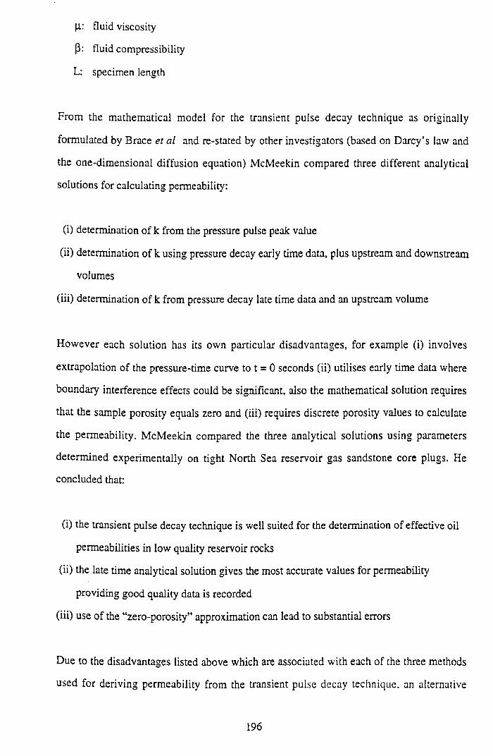
(i.: fluid viscosity

P: fluid compressibility

L: specimen length

From the mathematical model for the transient pulse decay technique as originally

formulated by Brace et al and re-stated by other investigators (based on Darcy’s law and

the one-dimensional diffusion equation) McMeekin compared three different analytical

solutions for calculating permeability:

(i) determination of k from the pressure pulse peak value

(ii) determination of k using pressure decay early time data, plus upstream and downstream

volumes

(iii) determination of k from pressure decay late time data and an upstream volume

However each solution has its own particular disadvantages, for example (i) involves

extrapolation of the pressure-time curve to t = 0 seconds (ii) utilises early time data where

boundary interference effects could be significant, also the mathematical solution requires

that the sample porosity equals zero and (iii) requires discrete porosity values to calculate

the permeability. McMeekin compared the three analytical solutions using parameters

determined experimentally on tight North Sea reservoir gas sandstone core plugs. He

concluded that:

(i) the transient pulse decay technique is well suited for the determination of effective oil

permeabilities in low quality reservoir rocks

(ii) the late time analytical solution gives the most accurate values for permeability

providing good quality data is recorded

(iii) use of the “zero-porosity” approximation can lead to substantial errors

Due to the disadvantages listed above which are associated with each of the three methods

used for deriving permeability from the transient pulse decay technique, an alternative

196

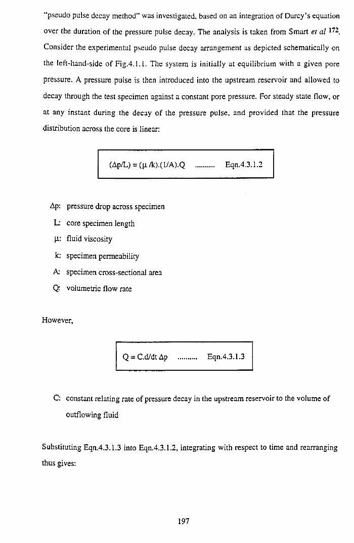
“pseudo pulse decay method” was investigated, based on an integration of Darcy’s equation

over the duration of the pressure pulse decay. The analysis is taken from Smart et a l 172.

Consider the experimental pseudo pulse decay arrangement as depicted schematically on

the left-hand-side of Fig.4.1.1. The system is initially at equilibrium with a given pore

pressure. A pressure pulse is then introduced into the upstream reservoir and allowed to

decay through the test specimen against a constant pore pressure. For steady state flow, or

at any instant during the decay of the pressure pulse, and provided that the pressure

distribution across the core is linear:

(Ap/L) = (|i/k).(l/A ).Q .......... Eqn.4.3.1.2

Ap: pressure drop across specimen

L: core specimen length

Ji: fluid viscosity

k: specimen permeability

A: specimen cross-sectional area

Q. volumetric flow rate

However,

Q = C.d/dt Ap .......... Eqn.4.3.1.3

C: constant relating rate of pressure decay in the upstream reservoir to the volume of

outflowing fluid

Substituting Eqn.4.3.1.3 into Eqn.4.3.1.2, integrating with respect to time and rearranging

thus gives:

197

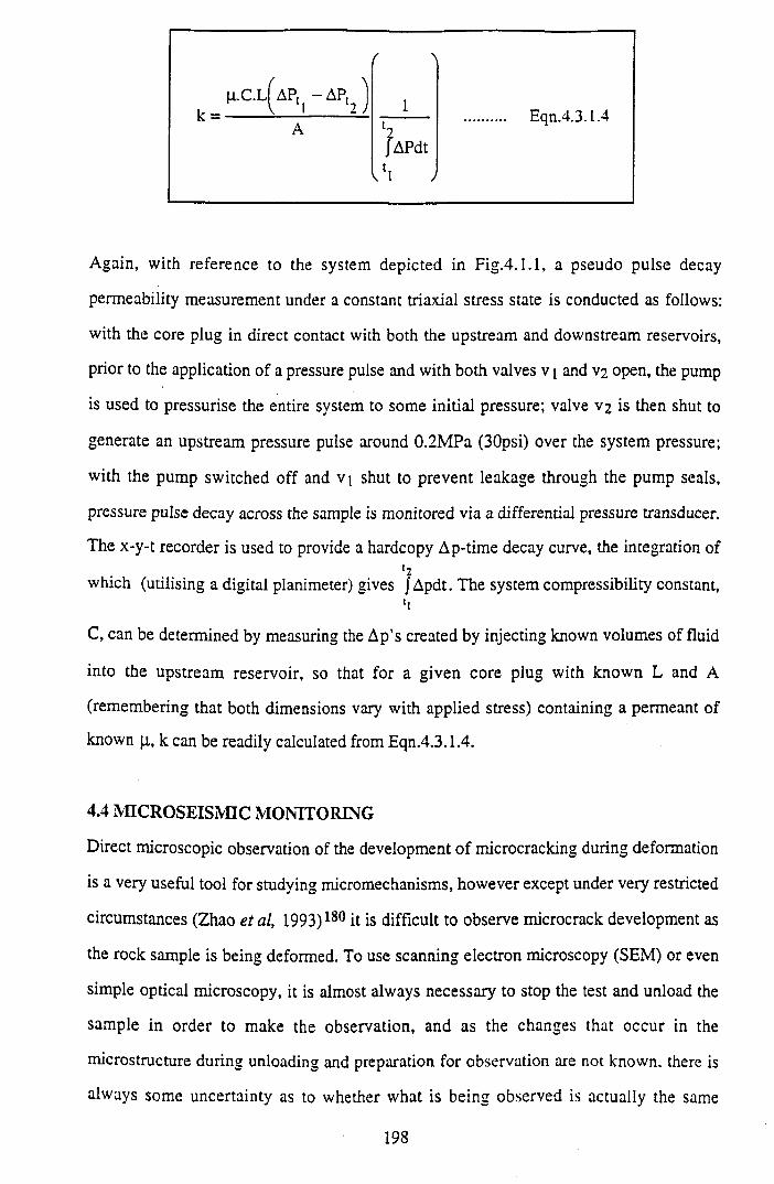
Again, with reference to the system depicted in F ig .4 .1.1, a pseudo pulse decay

permeability measurement under a constant triaxial stress state is conducted as follows:

with the core plug in direct contact with both the upstream and downstream reservoirs,

prior to the application of a pressure pulse and with both valves v i and V2 open, the pump

is used to pressurise the entire system to some initial pressure; valve V2 is then shut to

generate an upstream pressure pulse around 0.2MPa (30psi) over the system pressure;

with the pump switched off and v j shut to prevent leakage through the pump seals,

pressure pulse decay across the sample is monitored via a differential pressure transducer.

The x-y-t recorder is used to provide a hardcopy Ap-time decay curve, the integration of*2

which (utilising a digital planimeter) gives jApdt. The system compressibility constant,'!

C, can be determined by measuring the Ap’s created by injecting known volumes of fluid

into the upstream reservoir, so that for a given core plug with known L and A

(remembering that both dimensions vary with applied stress) containing a permeant of

known k can be readily calculated from Eqn.4.3.1.4.

4.4 M ICRO SEISM IC MONITORING

Direct microscopic observation of the development of microcracking during deformation

is a very useful tool for studying micromechanisms, however except under very restricted

circumstances (Zhao et al, 1993)180 it is difficult to observe microcrack development as

the rock sample is being deformed. To use scanning electron microscopy (SEM) or even

simple optical microscopy, it is almost always necessary to stop the test and unload the

sample in order to make the observation, and as the changes that occur in the

microstructure during unloading and preparation for observation are not known, there is

always some uncertainty as to whether what is being observed is actually the same

198

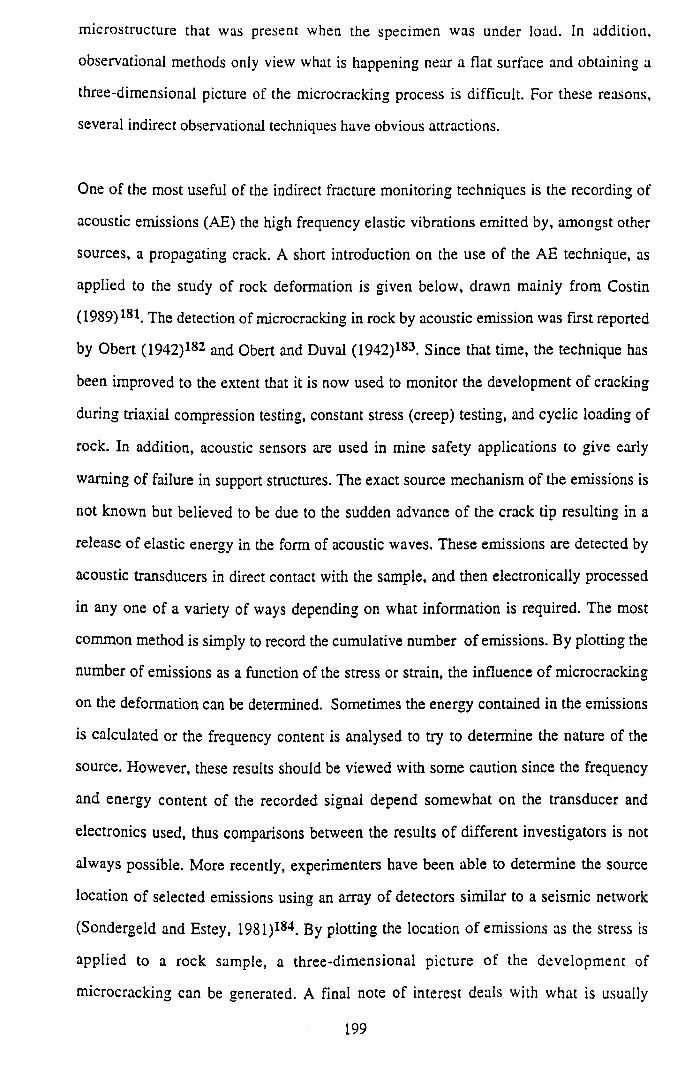
microstructure that was present when the specimen was under load. In addition,

observational methods only view what is happening near a flat surface and obtaining a

three-dimensional picture of the microcracking process is difficult. For these reasons,

several indirect observational techniques have obvious attractions.

One of the most useful of the indirect fracture monitoring techniques is the recording of

acoustic emissions (AE) the high frequency elastic vibrations emitted by, amongst other

sources, a propagating crack. A short introduction on the use of the AE technique, as

applied to the study of rock deformation is given below, drawn mainly from Costin

(1989)181. The detection of microcracking in rock by acoustic emission was first reported

by Obert (1942)182 and Obert and Duval (1942)183. Since that time, the technique has

been improved to the extent that it is now used to monitor the development o f cracking

during triaxial compression testing, constant stress (creep) testing, and cyclic loading of

rock. In addition, acoustic sensors are used in mine safety applications to give early

warning of failure in support structures. The exact source mechanism of the emissions is

not known but believed to be due to the sudden advance of the crack tip resulting in a

release of elastic energy in the form of acoustic waves. These emissions are detected by

acoustic transducers in direct contact with the sample, and then electronically processed

in any one of a variety of ways depending on what information is required. The most

common method is simply to record the cumulative number of emissions. By plotting the

number of emissions as a function of the stress or strain, the influence o f microcracking

on the deformation can be determined. Sometimes the energy contained in the emissions

is calculated or the frequency content is analysed to try to determine the nature of the

source. However, these results should be viewed with some caution since the frequency

and energy content of the recorded signal depend somewhat on the transducer and

electronics used, thus comparisons between the results o f different investigators is not

always possible. More recently, experimenters have been able to determine the source

location of selected emissions using an array of detectors similar to a seismic network

(Sondergeld and Estey, 1981)184. By plotting the location of emissions as the stress is

applied to a rock sample, a three-dimensional picture of the developm ent of

microcracking can be generated. A final note of interest deals with what is usually

199

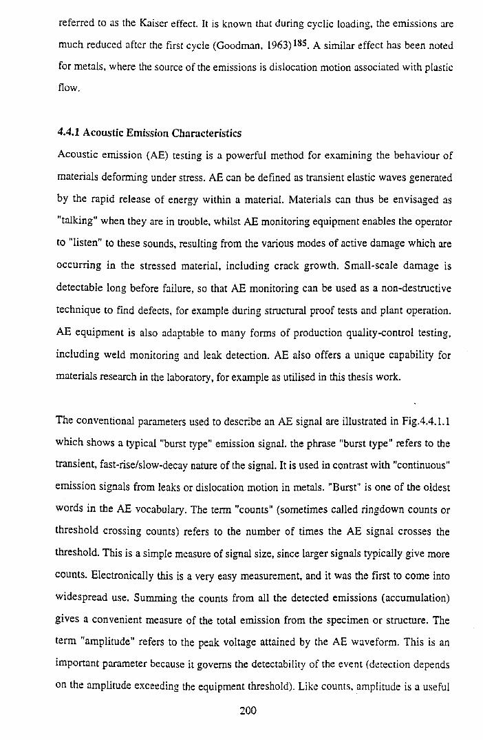
referred to as the Kaiser effect. It is known that during cyclic loading, the emissions are

much reduced after the first cycle (Goodman, 1963)185. a similar effect has been noted

for metals, where the source of the emissions is dislocation motion associated with plastic

flow.

4.4.1 Acoustic Emission Characteristics

Acoustic emission (AE) testing is a powerful method for examining the behaviour of

materials deforming under stress. AE can be defined as transient elastic waves generated

by the rapid release of energy within a material. Materials can thus be envisaged as

"talking" when they are in trouble, whilst AE monitoring equipment enables the operator

to "listen" to these sounds, resulting from the various modes of active damage which are

occurring in the stressed material, including crack growth. Small-scale damage is

detectable long before failure, so that AE monitoring can be used as a non-destructive

technique to find defects, for example during structural proof tests and plant operation.

AE equipment is also adaptable to many forms of production quality-control testing,

including weld monitoring and leak detection. AE also offers a unique capability for

materials research in the laboratory, for example as utilised in this thesis work.

The conventional parameters used to describe an AE signal are illustrated in Fig.4.4.1.1

which shows a typical "burst type" emission signal, the phrase "burst type" refers to the

transient, fast-rise/slow-decay nature of the signal. It is used in contrast with "continuous"

emission signals from leaks or dislocation motion in metals. "Burst" is one of the oldest

words in the AE vocabulary. The term "counts" (sometimes called ringdown counts or

threshold crossing counts) refers to the number of times the AE signal crosses the

threshold. This is a simple measure of signal size, since larger signals typically give more

counts. Electronically this is a very easy measurement, and it was the first to come into

widespread use. Summing the counts from all the detected emissions (accumulation)

gives a convenient measure of the total emission from the specimen or structure. The

term "amplitude" refers to the peak voltage attained by the AE waveform. This is an

important parameter because it governs the detectability of the event (detection depends

on the amplitude exceeding the equipment threshold). Like counts, amplitude is a useful

2 0 0

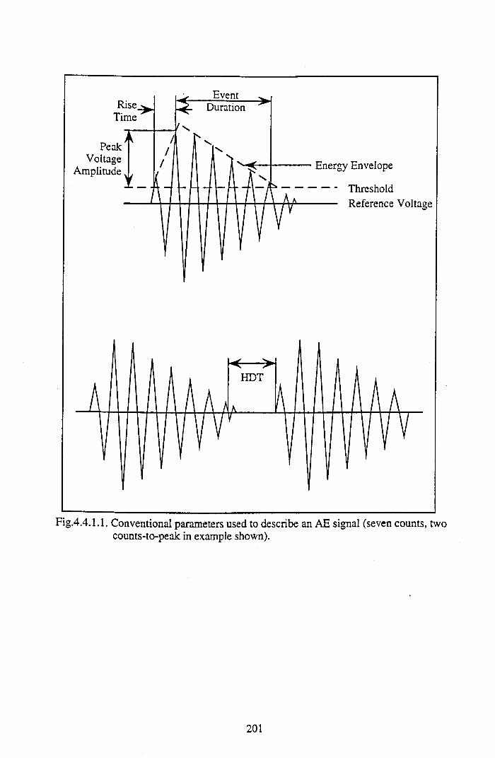
Fig.4.4.1.1. Conventional parameters used to describe an AE signal (seven counts, two counts-to-peak in example shown).

201

measure of signal size, and it is the appropriate variable to use for attenuation

measurements. Amplitude is conventionally expressed in decibels relative to one

microvolt at the sensor, the same scale that is used to specify threshold. This scale

converts the wide range of observed signal voltages (from a few microvolts to hundreds

o f millivolts) into convenient numbers between 0 and 100 :

Events with amplitudes <35dB are considered small

Events with amplitudes 35-55dB are considered medium-sized

Events with amplitudes 55-75dB are considered large

Events with amplitudes >75dB are considered very large

To accommodate the very wide dynamic range between the smallest and largest signals

encountered in actual testing, amplitude measurements are often made through a

logarithmic amplifier. This is placed in parallel with the linear amplifier that serves for

the other measurements. "Energy counts" describes the measured area under the rectified

signal envelope (also known as MARSE). This measurement requires relatively complex

circuitry, but it has the advantage that it is responsive to both the height (amplitude) and

width (duration) of the signal. As with ringdown counts, a convenient measure of the

total AE from a structure can be obtained by summing (accumulating) the energy counts

o f the individual signals. The parameter "duration" refers to the time from the first to the

last threshold crossing. This parameter is closely related to ringdown counts, but it is used

more for discrimination that for the measurement of emission quantities. Signals from

electromagnetic interference typically have very short durations, so this can be used to

filter them out. The "risetime" is the time from the first threshold crossing to the signal

peak. This parameter is useful for source discrimination and signal filtering. It can be

used to filter out signals from electromagnetic interference which usually have very short

risetimes. Also, it depends in a useful way on the distance wave propagation effects. So

to selectively monitor a known defect right under the sensor, a filter can be set to

eliminate acoustic signals coming from further away.

202

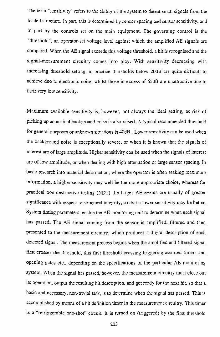
The term "sensitivity" refers to the ability o f the system to detect small signals from the

loaded structure. In part, this is determined by sensor spacing and sensor sensitivity, and

in part by the controls set on the main equipment. The governing control is the

"threshold", an operator-set voltage level against which the amplified AE signals are

compared. When the AE signal exceeds this voltage threshold, a hit is recognised and the

signal-measurement circuitry comes into play. W ith sensitivity decreasing with

increasing threshold setting, in practice thresholds below 20dB are quite difficult to

achieve due to electronic noise, whilst those in excess of 65dB are unattractive due to

their very low sensitivity.

Maximum available sensitivity is, however, not always the ideal setting, as risk of

picking up acoustical background noise is also raised. A typical recommended threshold

for general purposes or unknown situations is 40dB. Lower sensitivity can be used when

the background noise is exceptionally severe, or when it is known that the signals of

interest are of large amplitude. Higher sensitivity can be used when the signals of interest

are of low amplitude, or when dealing with high attenuation or large sensor spacing. In

basic research into material deformation, where the operator is often seeking maximum

information, a higher sensitivity may well be the more appropriate choice, whereas for

practical non-destructive testing (NDT) the larger AE events are usually o f greater

significance with respect to structural integrity, so that a lower sensitivity may be better.

System timing parameters enable the AE monitoring unit to determine when each signal

has passed. The AE signal coming from the sensor is amplified, filtered and then

presented to the measurement circuitry, which produces a digital description of each

detected signal. The measurement process begins when the amplified and filtered signal

first crosses the threshold, this first threshold crossing triggering assorted timers and

opening gates etc., depending on the specifications of the particular AE monitoring

system. When the signal has passed, however, the measurement circuitry must close out

its operation, output the resulting hit description, and get ready for the next hit, so that a

basic and necessary, non-trivial task, is to determine when the signal has passed. This is

accomplished by means of a hit definition timer in the measurement circuitry. This timer

is a “retriggerable one-shot” circuit. It is turned on (triggered) by the first threshold

203

Crossing, and retriggered by each new threshold crossing. It turns off, terminating the

measurement process, when the “hit definition time” (HDT) has expired without any

more triggerings (threshold crossings). The HDT is selected by the operator before the

test. When a suitable value is selected, each acoustic emission will produce a single hit

description in a timely manner. If the HDT is set too low, the timer may expire in the

middle of the signal, and the system will treat the next part of the signal as a separate

event, producing invalid data. If the HDT is set too high, a separate event may be

included along with the first in a single hit description, also resulting in invalid data.

Whilst the function of the HDT is to enable the system to determine the end of the hit.

close out the measurement process and store the measured attributes of the signal, the

function of the “peak definition time” (PDT) is to enable determination of the time of the

true peak of the AE waveform. For PDT, the main requirement is to avoid false

measurements being made on a high-velocity, low-amplitude precursor, so that ideally,

PDT should be set as short as possible. The function of “hit lockout time” (HLT) is to

inhibit the measurement of reflections and late-arriving parts of the AE signal, so that

data from wave arrivals can be acquired at a faster rate.

4.4.2 The LOCAN-320 AE Monitoring Unit

The LOCAN-320 is a computerised AE monitoring system supplied by the Physical

Acoustics Corporation (PAC) that performs AE signal measurements and stores, displays

and analyses the resulting data in real time. The AE signals from the loaded structure

(confined rock specimen) are converted into electrical signals by the sensors, amplified to

usable voltage levels by the preamplifiers and measured in two-channel computerised

modules known as Independent Channel Controllers (ICC's). Each AE signal (hit) is

described in terms of various measured parameters as outlined above. Other variables

such as time of occurrence or load on the structure at thé time the event occurred are also

included in the hit description. Hit descriptions are stored in the output of the ICC until

the system's main processor is ready to run them. The Standard LOCAN-320 system

hardware design incorporates a modular architecture that contains an analogue interface

and pre-processor bus organiser, as well as channel controller and parametric channel

controller under the control of a multibus based microprocessor. The requirements of

204

high-speed data acquisition have been separated from the more complex requirements of

analysis and display, with the result that substantially faster data acquisition, with more

information about each event can be achieved. The dual bus structure separates tasks

between processors, allowing the IBM-PC to process and present graphical displays, and

the multibus to acquire and extract the appropriate features from the AE signals. The ICC

is a single board, two channel AE computer which utilises the dual-bus architecture of the

LOCAN-320 to communicate with the main processor. The ICC performs signal feature

extraction, temporary hit buffering (>1000 hits) and front-end data filtering. The buffer

data is immediately available to the host computer (80286) for processing and real-time

graphics. The basic standard application software package supplied with every LOCAN-

320 serves for setting up channel parameters, real-time graphics, conditioning alarms,

filtering, testing, file handling, acquisition start and replay.

The most important single factor in successfully performing an AE application is the

reliability of the AE sensor. As an AE sensor converts the mechanical energy carried by

the elastic wave into an electrical signal, the sensor is more properly termed a transducer.

The transducer most often used in AE applications is the piezoelectric transducer. This

choice has been dictated by its inherently high sensitivity and relative ruggedness. The

active element of a piezoelectric transducer is a thin disk of piezoelectric material (a

material which can convert mechanical deformation into electrical voltage). This disk is

metallized on both faces for electrical contact, and mounted in a metal cylinder to provide

electromagnetic interference shielding. The piezoelectric ceramics commonly used in AE

transducers are made of small crystals of titanates and zirconates which are mixed with

other materials, moulded to the desired shape, and fired in a kiln. The ceramic material is

then made piezoelectric by poling, which is the process of heating the material above its

Curie temperature whilst under a strong electric field. To take advantage of the extreme

sensitivity of the piezoelectric transducer, it must be attached to the material under

observation in such a manner that the acoustic energy passes into the transducer with

minimum loss at the transducer-material interface. The required intimate mechanical

contact is achieved on flat surfaces by mechanical clamping using thin films of grease, oil

or epoxy adhesive between the transducer and the material. In general, the problem of

205

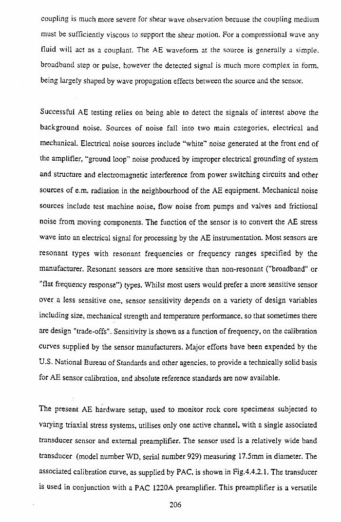
coupling is much more severe for shear wave observation because the coupling medium

must be sufficiently viscous to support the shear motion. For a compressional wave any

fluid will act as a couplant. The AE waveform at the source is generally a simple,

broadband step or pulse, however the detected signal is much more complex in form,

being largely shaped by wave propagation effects between the source and the sensor.

Successful AE testing relies on being able to detect the signals of interest above the

background noise. Sources of noise fall into two main categories, electrical and

mechanical. Electrical noise sources include “white” noise generated at the front end ot

the amplifier, “ground loop” noise produced by improper electrical grounding of system

and structure and electromagnetic interference from power switching circuits and other

sources of e.m. radiation in the neighbourhood of the AE equipment. Mechanical noise

sources include test machine noise, flow noise from pumps and valves and frictional

noise from moving components. The function of the sensor is to convert the AE stress

wave into an electrical signal for processing by the AE instrumentation. Most sensors are

resonant types with resonant frequencies or frequency ranges specified by the

manufacturer. Resonant sensors are more sensitive than non-resonant ("broadband" or

"flat frequency response”) types. Whilst most users would prefer a more sensitive sensor

over a less sensitive one, sensor sensitivity depends on a variety of design variables

including size, mechanical strength and temperature performance, so that sometimes there

are design "trade-offs". Sensitivity is shown as a function of frequency, on the calibration

curves supplied by the sensor manufacturers. Major efforts have been expended by the

U.S. National Bureau of Standards and other agencies, to provide a technically solid basis

for AE sensor calibration, and absolute reference standards are now available.

The present AE hardware setup, used to monitor rock core specimens subjected to

varying triaxial stress systems, utilises only one active channel, with a single associated

transducer sensor and external preamplifier. The sensor used is a relatively wide band

transducer (model number WD, serial number 929) measuring 17.5mm in diameter. The

associated calibration curve, as supplied by PAC, is shown in Fig.4.4.2.1. The transducer

is used in conjunction with a PAC 1220A preamplifier. This preamplifier is a versatile

206

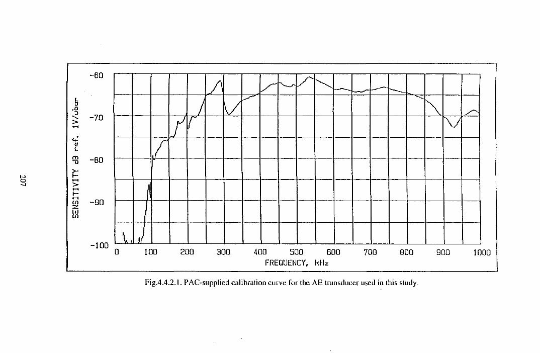
-60

Fig.4.4.2.1. PAC-suppIied calibration curve for the AE transducer used in this study.

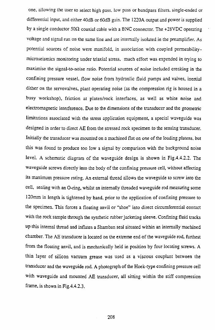
one, allowing the user to select high pass, low pass or bandpass filters, single-ended or

differential input, and either 40dB or 60dB gain. The 1220A output and power is supplied

by a single conductor 50Q coaxial cable with a BNC connector. The +28VDC operating

voltage and signal run on the same line and are internally isolated in the preamplifier. As

potential sources of noise were manifold, in association with coupled permeability-

microseismics monitoring under triaxial stress, much effort was expended in trying to

maximise the signal-to-noise ratio. Potential sources of noise included creaking in the

confining pressure vessel, flow noise from hydraulic fluid pumps and valves, inertial

dither on the servovalves, plant operating noise (as the compression rig is housed in a

busy workshop), friction at platen/rock interfaces, as well as white noise and

electromagnetic interference. Due to the dimensions of the transducer and the geometric

limitations associated with the stress application equipment, a special waveguide was

designed in order to direct AE from the stressed rock specimen to the sensing transducer.

Initially the transducer was mounted on a machined flat on one of the loading platens, but

this was found to produce too low a signal by comparison with the background noise

level. A schematic diagram of the waveguide design is shown in Fig.4.4.2.2. The

waveguide screws directly into the body of the confining pressure cell, without affecting

its maximum pressure rating. An external thread allows the waveguide to screw into the

cell, sealing with an O-ring, whilst an internally threaded waveguide rod measuring some

120mm in length is tightened by hand, prior to the application of confining pressure to

the specimen. This forces a floating anvil or “shoe” into direct circumferential contact

with the rock sample through the synthetic rubber jacketing sleeve. Confining fluid tracks

up this internal thread and inflates a Shamban seal situated within an internally machined

chamber. The AE transducer is located on the extreme end of the waveguide rod, furthest

from the floating anvil, and is mechanically held in position by four locating screws. A

thin layer of silicon vacuum grease was used as a viscous couplant between the

transducer and the waveguide rod. A photograph of the Hoek-type confining pressure cell

with waveguide and mounted AE transducer, all sitting within the stiff compression

frame, is shown in Fig.4.4.2.3.

208

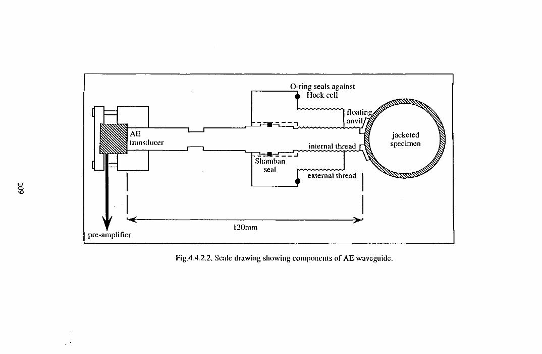
Fig.4.4.2.2. Scale drawing showing components of AE waveguide.

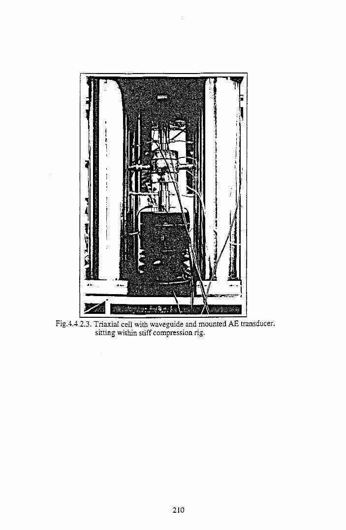
Fig.4.4.2.3. Triaxial cell with waveguide and mounted AE transducer, sitting within stiff compression rig.

2 1 0

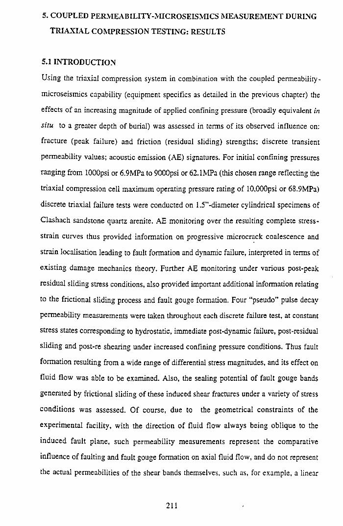
5. COUPLED PERMEABILITY-MICROSEISMICS MEASUREMENT DURING

TRIAXIAL COMPRESSION TESTING: RESULTS

5.1 INTRODUCTION

Using the triaxial compression system in combination with the coupled permeability -

microseismics capability (equipment specifics as detailed in the previous chapter) the

effects of an increasing magnitude of applied confining pressure (broadly equivalent in

situ to a greater depth of burial) was assessed in terms of its observed influence on:

fracture (peak failure) and friction (residual sliding) strengths; discrete transient

permeability values; acoustic emission (AE) signatures. For initial confining pressures

ranging from lOOOpsi or 6.9MPa to 9000psi or 62.1MPa (this chosen range reflecting the

triaxial compression cell maximum operating pressure rating of 10,000psi or 68.9MPa)

discrete triaxial failure tests were conducted on 1.5”-diameter cylindrical specimens of

Clashach sandstone quartz arenite. AE monitoring over the resulting complete stress -

strain curves thus provided information on progressive microcrack coalescence and

strain localisation leading to fault formation and dynamic failure, interpreted in terms of

existing damage mechanics theory. Further AE monitoring under various post-peak

residual sliding stress conditions, also provided important additional information relating

to the frictional sliding process and fault gouge formation. Four “pseudo” pulse decay

permeability measurements were taken throughout each discrete failure test, at constant

stress states corresponding to hydrostatic, immediate post-dynamic failure, post-residual

sliding and post-re shearing under increased confining pressure conditions. Thus fault

formation resulting from a wide range of differential stress magnitudes, and its effect on

fluid flow was able to be examined. Also, the sealing potential of fault gouge bands

generated by frictional sliding of these induced shear fractures under a variety of stress

conditions was assessed. Of course, due to the geometrical constraints of the

experimental facility, with the direction of fluid flow always being oblique to the

induced fault plane, such permeability measurements represent the comparative

influence of faulting and fault gouge formation on axial fluid flow, and do not represent

the actual permeabilities of the shear bands themselves, such as, for example, a linear

211

flow cell measurement does for a proppant bed. “Post-mortem” particle sizing analyses

of the fault gouge samples formed by these discrete discontinuity triaxial compression

tests are reported in Chapter 6 . There, emphasis is placed on the establishment of

empirical relations between the size distributions of the different fault gouge samples,

and their associated frictional strength and fluid flow characteristics as described in this

chapter.

5.2 EXPERIMENTAL METHODOLOGY

Whilst in Chapter 3 the main objective was to investigate the effects of constant normal

displacement boundary conditions on the direct shear response of a variety of lithologies,

that is to study the influence of rock type on frictional strength, in the discontinuity

triaxial compression tests described below, the primary variable under scrutiny was the

magnitude of applied triaxial stress, so that ideally, initial pre-stress microstructure

should be as constant as possible between test specimens. To this end, Clashach

sandstone was chosen as being the most readily available reservoir sandstone analogue

possessing this quality, that is being sufficiently homogeneous and isotropic on a

quarried block scale so as to provide core plugs with a minimum of between-sample

variation.

The Clashach sandstone is a commercially available Permo-Triassic sandstone sourced

from a quarry in Elgin, Scotland. It is a pale-fawn, well-sorted, medium- to coarse­

grained (0.5-1mm) quartz arenite with well-developed quartz overgrowths. X-ray

diffraction (XRD) analysis shows quartz content ranging from 90 to 96%, K-feldspar

constituting the remaining modal percent, and trace amounts of illite (Ngwenya ex al,

1993)186. Occasional thin-sections also show very minor development of ferroan

dolomite and kaolinite. Ngwenya also notes that permeability measurements conducted

under hydrostatic conditions on different Clashach sandstone specimens proved variable,

ranging from 200mD to ID, the lower permeability samples in general showing a more

reddish colour, suggestive of the observed variation being the result of pore-throat

blockage by ferric compounds. Mineralogical, poroperm and rock mechanical parameters

212

determined from a programme of characterisation conducted on the Clashach sandstone

core specimen source-block used for this suite of tests, are detailed in Table 5.2.1. Elastic

constants were measured from uniaxial compression of 1.5”-diameter (38mm) strain-

gauged core plugs, which were subsequently taken to failure to determine unconfined

strengths. Tensile strengths were evaluated using the Brazilian disk indirect method. The

theoretical and empirical failure criteria constants were determined using the multi­

failure state triaxial method to generate ten Mohr circles from a single specimen at

confining pressures ranging from lOOOpsi (6.9MPa) to 10 OOOpsi (68.9MPa).

Due to the relatively complex nature of the experimental procedure, over twenty discrete

triaxial tests were run with a success rate of 30%, before the maximum range of stress

magnitudes was achieved. The main problems encountered were those of perforated

triaxial cell liners due to excessive sliding displacements, poor AE coupling prior to the

waveguide installation, and initial “teething” problems associated with proving of the

pseudo pulse decay method, such as permeant leakage. The Clashach core plugs

consisted of 1.5 inch-diameter (38mm) right circular cylinders 3.1 inches in length,

giving a length-to-diameter ratio in excess of 2:1. Specimen ends were prepared flat and

parallel to within ISRM specifications (Vogler & K o v a r i^ ) using a lathe as opposed to

a lapping jig, in order to m inim ise damage and “skin effects” which would influence

fluid flow.

The triaxial compression system with coupled permeability-microseismics facility used

for this suite of tests, is as illustrated schematically in Fig.4.1.1. Starting from ambient

atmospheric conditions, each specimen was taken to an initial pre-determined hydrostatic

stress state by increasing both axial load and confining pressure in step. Axial load was

then increased over constant confining pressure (thus <Ja = G l and p=cr 3 ) under

displacement control and at a constant displacement rate equivalent to a strain rate of

1.6X10-V1. Fig.5.2.1 illustrates schematically the experimental test programme that each

specimen was subjected to, with of course the magnitude of the initial hydrostatic stress

being the main variable under examination. From Fig.5 .2 .1 it is evident that whilst

213

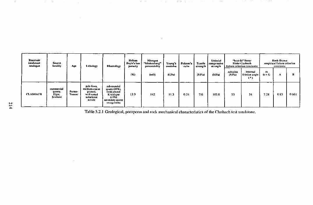
214

Reservoirsandstoneanalogue

Sourcelocality Age l.ithology Mineralogy

Helium Boyle's law

porusity

Nitrogen“ klinkenberg"

permeabilityYoung'smodulus

Poisson'sratio

Tensilestrength

Uniaxialcompressive

strength

“best-fit" linear Mohr-Coulomb

failure criterion constants:

Hoek-Brownempirical failure criterion

constants:

(%> (ml)) («Pa) (MPa) (MPa)cohesion(MPa)

internal friction angle

( ° )

m(s = l) A B

CI.ASIIACH

commercialquarry,Elgin.

Scotland

Pcrmo-Triassic

pale-fawn,medium-coarse

grained,well-sortedsubarkosic

arenile

sub-rounded qua ru (89%), fresh-altered K-feldspar

(11%)secondary quartz

overgiowtlis

13.9 142 11.3 0 2 4 7.6 105.« 53 34 7.28 0,83 0 661

Table 5.2.1 Geological, poroperm and rock mechanical characteristics of the Clashach test sandstone.

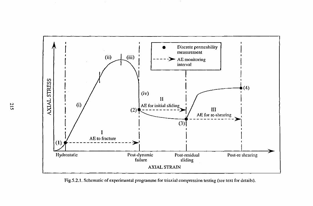
Fig.5.2.1. Schematic of experimental programme for triaxial compression testing (see text for details).

discrete permeability measurements were conducted under constant stress states, AE

was monitored over conditions of changing stress associated with a constant applied

strain rate. As noted in the introduction, four “pseudo” pulse decay permeability

measurements were made throughout each discrete failure test, under constant stress

conditions corresponding to: (1) hydrostatic; (2) immediate post-dynamic failure; (3)

post-residual sliding; (4) post re-shearing under increased confining pressure conditions.

The aim of such an experimental method was to assess the effects of fault formation, and

of progressive dynamic fragmentation resulting in shear debris (fault gouge) generation,

on axial plug flow occurring in the same rock type but at stresses corresponding to

different depths in the Earth’s crust. Also, it was hoped that the hydrostatic

measurements would allow normalisation of those permeabilities recorded under post-

faulting stress conditions, thus offering some means of compensating for between-

sample variability and for elastic stress-sensitivity. Three different AE signatures were

recorded under varying stress test conditions corresponding to: (I) taking the initially

intact core specimen from hydrostatic stress, over its complete failure cycle, to a faulted

state; (II) sliding the induced shear fracture for a pre-determined displacement to a

residual strength state; (III) further sliding the faulted specimen under an altered stress

state achieved by increasing the confining pressure by an arbitrary lOOOpsi (6.9MPa)

thus re-shearing the fault under an artificially strengthened state. In summary, AE (I) was

measured over varying stress conditions from that associated with permeability ( 1) to

that associated with permeability (2), AE (II) from permeability (2) to permeability (3)

and AE (HI) from permeability (3) to permeability (4). The aim of the AE experimental

procedure was to allow a comparison of acoustic properties (in constant-lithology

systems but corresponding to different depths in the Earth’s crust) during: (I) the

nucleation phase of faulting; (II) initial sliding of the fault after quasi-static and dynamic

slip-weakening followed by; (III) a longer-term recovery in frictional strength. The

mechanical strengthening effect resulting from increasing the normal stress across the

fault by increasing the confining pressure, mimics to some extent the quasi-static

strength recovery which can occur in the Earth from combined physico-chemical

processes over longer timescales and with a more reactive pore fluid, namely pressure

216

solution “crack-seal” (Ramsay, 1980187) and dilatancy hardening (Brace & Martin.

1968188). In Fig.5.2.1 AE (I) is further subdivided into: (i) a linear quasi-elastic phase;

(ii) a strain hardening phase up to the peak strength of the material; (iii) a stable strain

softening phase; (iv) dynamic stress drop. Phase (i) is termed “quasi-elastic” since,

although axial stress and strain are related in a linear manner, local inelastic processes

resulting in AE are also characteristic.

In total seven Clashach sandstone specimens were tested, with initial hydrostatic stress

states ranging from lOOOpsi to 9000psi. For the “industry accepted” approximate

overburden stress gradient of l.Opsi/ft (Skopec, 1991189) and assuming a uniform

increase in overburden stress with depth, the limits of applied laboratory hydrostatic

stress correspond to depths extending from 1000ft (0.3km) to 9000ft (2.7km). Table

5.2.2 lists the hydrostatic stress magnitudes, equivalent to the confining pressures applied

during AE monitoring for stages (I) and (II), and the final confining pressures for AE

stage (III) and for permeability (4) following a lOOOpsi (6.9MPa) increase. From Table

5.2.2 it is evident that five specimens were tested under initial confining pressures of

1000, 3000, 5000, 7000 and 9000psi whilst a further two duplicate specimens were also

tested under 3000 and 9000psi pressures, to check data reproducibility.

5.3 STRENGTH RESULTS

Using the triaxial stress application system as described above, for the experimental

methodology as described above, the effect of initial specimen confinement on strength

measures was appraised. To this end, the main method of data recording was graphical

generation of axial load versus axial displacement profiles on an x-y-t chart recorder,

linked to a plotter drive unit within the servo-control system. From these curves any

axial load could be converted to an equivalent axial stress by dividing by the specimen

cross-sectional area, whilst the corresponding axial displacement could be converted to

an axial strain by dividing the change in specimen length by its initial pre-deformation

length and expressing the resultant in either microstrain or percent. Axial load-

displacement profiles from the seven triaxial tests conducted are shown in Fig.5.3.1. The

217

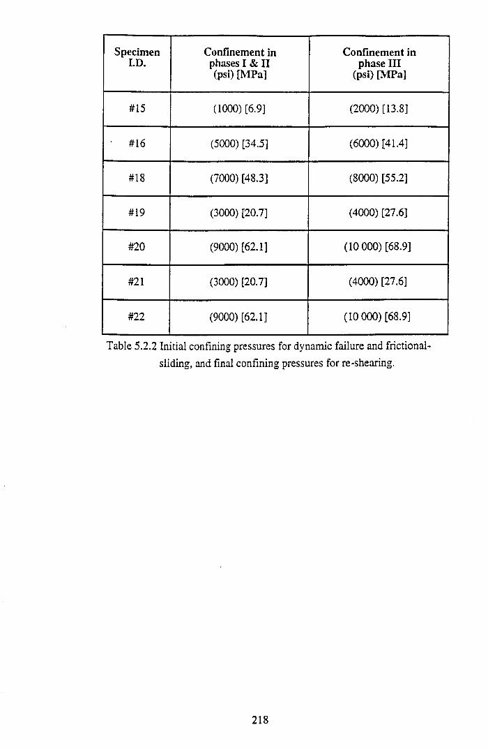
SpecimenI.D.

Confinement in phases I & II (psi) [MPa]

Confinement in phase III

(psi) [MPa]

#15 (1000) [6.9] (2000) [13.8]

#16 (5000) [34.5] (6000) [41.4]

#18 (7000)[48.3] (8000) [55.2]

#19 (3000) [20.7] (4000) [27.6]

# 20 (9000) [62.1] (10 000) [68.9]

#21 (3000) [20.7] (4000) [27.6]

#22 (9000) [62.1] (10 000) [68.9]

Table 5.2.2 Initial confining pressures for dynamic failure and frictional-

sliding, and final confining pressures for re-shearing.

218

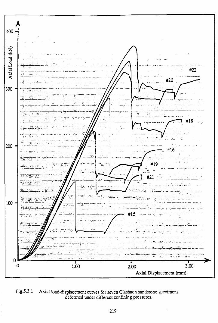
Fig-5.3.1 Axial load-displacement curves for seven Clashach sandstone specimensdeformed under different confining pressures.

219

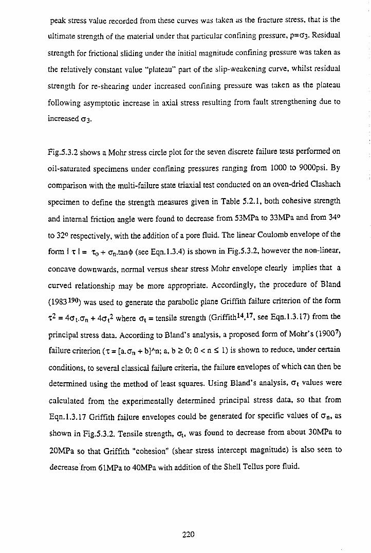
peak stress value recorded from these curves was taken as the fracture stress, that is the

ultimate strength of the material under that particular confining pressure, p= 0 ‘3. Residual

strength for frictional sliding under the initial magnitude confining pressure was taken as

the relatively constant value “plateau” part of the slip-weakening curve, whilst residual

strength for re-shearing under increased confining pressure was taken as the plateau

following asymptotic increase in axial stress resulting from fault strengthening due to

increased a 3.

Fig.5.3.2 shows a Mohr stress circle plot for the seven discrete failure tests performed on

oil-saturated specimens under confining pressures ranging from 1000 to 9000psi. By

comparison with the multi-failure state triaxial test conducted on an oven-dried Clashach

specimen to define the strength measures given in Table 5.2.1, both cohesive strength

and internal friction angle were found to decrease from 53MPa to 33MPa and from 34°

to 32° respectively, with the addition of a pore fluid. The linear Coulomb envelope of the

form 1 x 1 = x0 + crn.tan(|) (see Eqn. 1.3.4) is shown in Fig.5.3.2, however the non-linear,

concave downwards, normal versus shear stress Mohr envelope clearly implies that a

curved relationship may be more appropriate. Accordingly, the procedure of Bland

(1983li>0) was used to generate the parabolic plane Griffith failure criterion of the form

X2 = 4 a t.a n + 4 a t2 where a t = tensile strength (Griffith14,17, see Eqn. 1.3.17) from the

principal stress data. According to Bland’s analysis, a proposed form of Mohr’s (19007)

failure criterion (x = [a .an + b]An; a, b > 0 ; 0 < n < 1) is shown to reduce, under certain

conditions, to several classical failure criteria, the failure envelopes of which can then be

determined using the method of least squares. Using Bland’s analysis, a t values were

calculated from the experimentally determined principal stress data, so that from

Eqn. 1.3.17 Griffith failure envelopes could be generated for specific values of a n. as

shown in Fig.5.3.2. Tensile strength, at, was found to decrease from about 30MPa to

20MPa so that Griffith "cohesion" (shear stress intercept magnitude) is also seen to

decrease from 61MPa to 40MPa with addition of the Shell Tellus pore fluid.

220

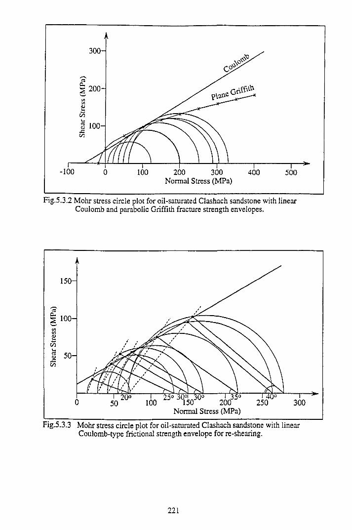
Fig.5.3.2 Mohr stress circle plot for oil-saturated Clashach sandstone with linear Coulomb and parabolic Griffith fracture strength envelopes.

Fig.5.3.3 Mohr stress circle plot for oil-saturated Clashach sandstone with linear Coulomb-type frictional strength envelope for re-shearing.

221

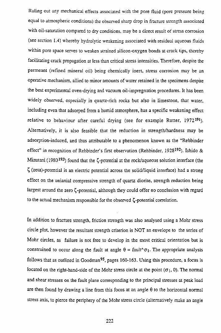
Ruling out any mechanical effects associated with the pore fluid (pore pressure being

equal to atmospheric conditions) the observed sharp drop in fracture strength associated

with oil-saturation compared to dry conditions, may be a direct result of stress corrosion

(see section 1.4) whereby hydrolytic weakening associated with residual aqueous fluids

within pore space serves to weaken strained silicon-oxygen bonds at crack tips, thereby

facilitating crack propagation at less than critical stress intensities. Therefore, despite the

permeant (refined mineral oil) being chemically inert, stress corrosion may be an

operative mechanism, allied to minor amounts of water retained in the specimens despite

the best experimental oven-drying and vacuum oil-impregnation procedures. It has been

widely observed, especially in quartz-rich rocks but also in limestone, that water,

including even that adsorped from a humid atmosphere, has a specific weakening effect

relative to behaviour after careful drying (see for example Rutter, 1972191).

Alternatively, it is also feasible that the reduction in strength/hardness may be

adsorption-induced, and thus attributable to a phenomenon known as the “Rehbinder

effect” in recognition of Rehbinder’s first observation (Rehbinder, 1928192). Ishido &

Mizutani (1980193) found that the ^-potential at the rock/aqueous solution interface (the

£ (zeta)-potential is an electric potential across the solid/liquid interface) had a strong

effect on the uniaxial compressive strength of quartz diorite, strength reduction being

largest around the zero ^-potential, although they could offer no conclusion with regard

to the actual mechanism responsible for the observed ^-potential correlation.

In addition to fracture strength, friction strength was also analysed using a Mohr stress

circle plot, however the resultant strength criterion is NOT an envelope to the series of

Mohr circles, as failure is not free to develop in the most critical orientation but is

constrained to occur along the fault at angle 0 = faultA<Ji. The appropriate analysis

follows that as outlined in Goodman93, pages 160-163. Using this procedure, a focus is

located on the right-hand-side of the Mohr stress circle at the point (a i, 0). The normal

and shear stresses on the fault plane corresponding to the principal stresses at peak load

are then found by drawing a line from this focus at an angle 0 to the horizontal normal

stress axis, to pierce the periphery of the Mohr stress circle (alternatively make an angle

222

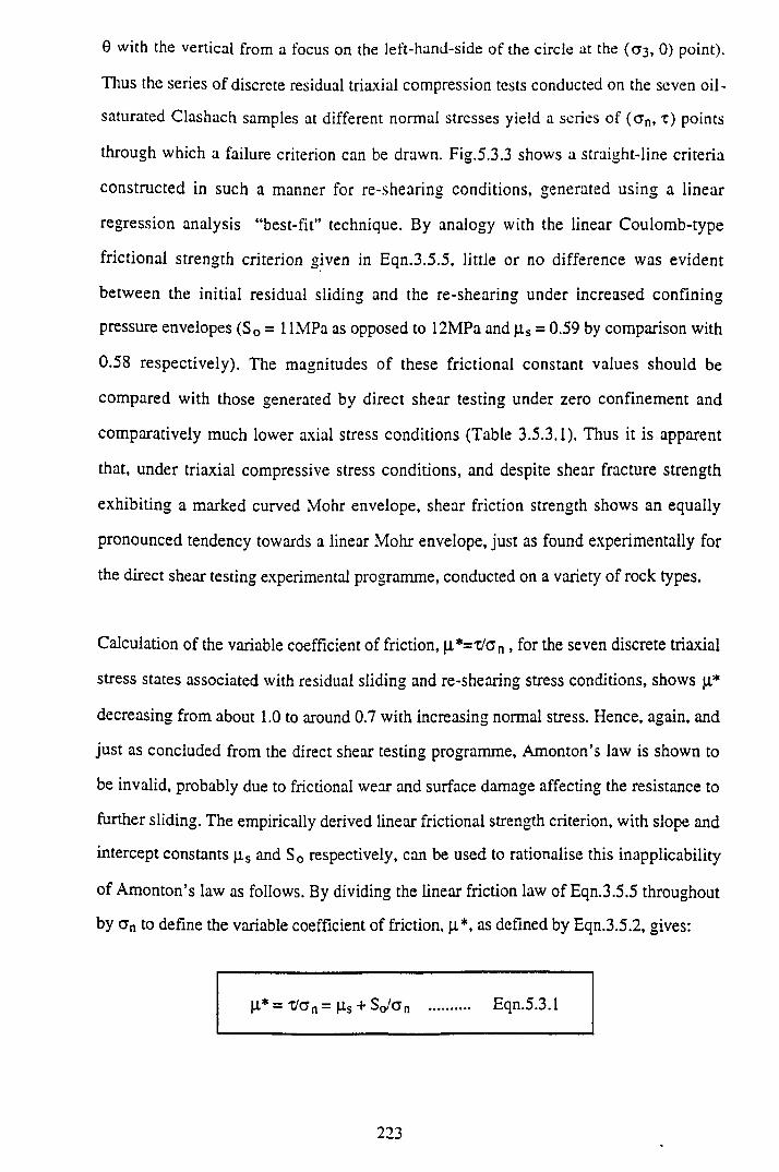
0 with the vertical from a focus on the left-hand-side of the circle at the ((73, 0 ) point).

Thus the series of discrete residual triaxial compression tests conducted on the seven oil -

saturated Clashach samples at different normal stresses yield a series of ( c n, t ) points

through which a failure criterion can be drawn. Fig.5.3.3 shows a straight-line criteria

constructed in such a manner for re-shearing conditions, generated using a linear

regression analysis “best-fit” technique. By analogy with the linear Coulomb-type

frictional strength criterion given in Eqn.3.5.5, littJe or no difference was evident

between the initial residual sliding and the re-shearing under increased confining

pressure envelopes (S0 = 1 IMPa as opposed to 12MPa and jis = 0.59 by comparison with

0.58 respectively). The magnitudes of these frictional constant values should be

compared with those generated by direct shear testing under zero confinement and

comparatively much lower axial stress conditions (Table 3.5.3.1). Thus it is apparent

that, under triaxial compressive stress conditions, and despite shear fracture strength

exhibiting a marked curved Mohr envelope, shear friction strength shows an equally

pronounced tendency towards a linear Mohr envelope, just as found experimentally for

the direct shear testing experimental programme, conducted on a variety of rock types.

Calculation of the variable coefficient of friction, |i* = t/a n , for the seven discrete triaxial

stress states associated with residual sliding and re-shearing stress conditions, shows |i*

decreasing from about 1.0 to around 0.7 with increasing normal stress. Hence, again, and

just as concluded from the direct shear testing programme, Amonton’s law is shown to

be invalid, probably due to frictional wear and surface damage affecting the resistance to

further sliding. The empirically derived linear frictional strength criterion, with slope and

intercept constants | i s and S0 respectively, can be used to rationalise this inapplicability

of Amonton’s law as follows. By dividing the linear friction law of Eqn.3.5.5 throughout

by a n to define the variable coefficient of friction, (!*, as defined by Eqn.3.5.2, gives:

|X* = x/on = |is + So/an .......... Eqn.5.3.1

223

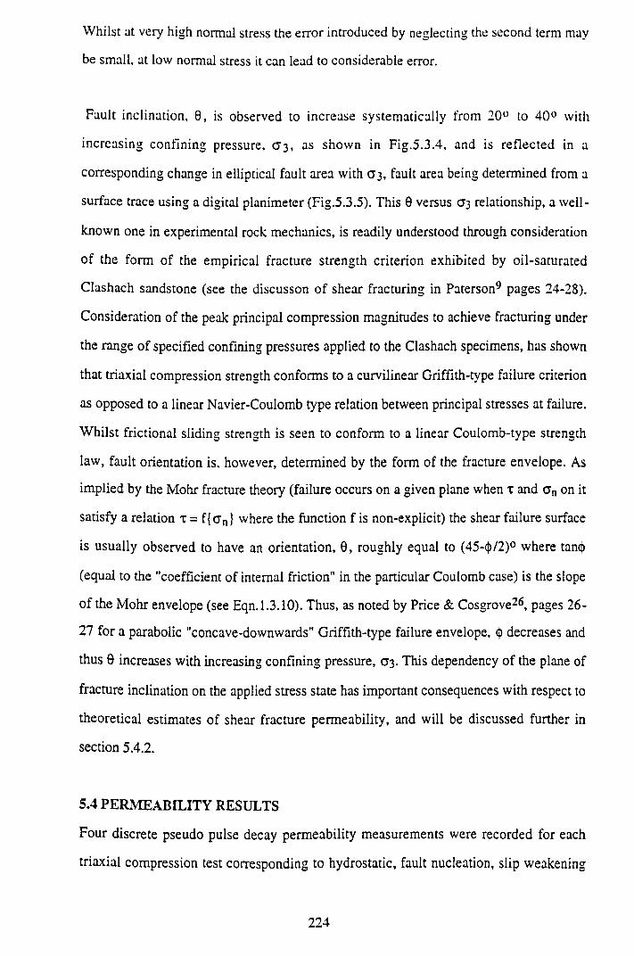
Whilst at very high normal stress the error introduced by neglecting the second term may

be small, at low normal stress it can lead to considerable error.

Fault inclination, 0, is observed to increase systematically from 20° to 40° with

increasing confining pressure, (7 3 , as shown in Fig.5.3.4, and is reflected in a

corresponding change in elliptical fault area with G3, fault area being determined from a

surface trace using a digital planimeter (Fig.5.3.5). This 0 versus CT3 relationship, a well-

known one in experimental rock mechanics, is readily understood through consideration

of the form of the empirical fracture strength criterion exhibited by oil-saturated

Clashach sandstone (see the discusson o f shear fracturing in Paterson^ pages 24-28).

Consideration of the peak principal compression magnitudes to achieve fracturing under

the range of specified confining pressures applied to the Clashach specimens, has shown

that triaxial compression strength conforms to a curvilinear Griffith-type failure criterion

as opposed to a linear Navier-Coulomb type relation between principal stresses at failure.

Whilst frictional sliding strength is seen to conform to a linear Coulomb-type strength

law, fault orientation is, however, determined by the form of the fracture envelope. As

implied by the Mohr fracture theory (failure occurs on a given plane when x and c n on it

sadsfy a relation x = f{ cn} where the function f is non-explicit) the shear failure surface

is usually observed to have an orientation, 0, roughly equal to (45-0/2)° where tancp

(equal to the "coefficient of internal friction" in the particular Coulomb case) is the slope

o f the Mohr envelope (see Eqn.1.3.10). Thus, as noted by Price & Cosgrove^, pages 26-

27 for a parabolic "concave-downwards" Griffith-type failure envelope, 0 decreases and

thus 0 increases with increasing confining pressure, (73. This dependency of the plane of

fracture inclination on the applied stress state has important consequences with respect to

theoretical estimates of shear fracture permeability, and will be discussed further in

section 5.4.2.

5.4 PERMEABILITY RESULTS

Four discrete pseudo pulse decay permeability measurements were recorded for each

triaxial compression test corresponding to hydrostatic, fault nucleadon, slip weakening

224

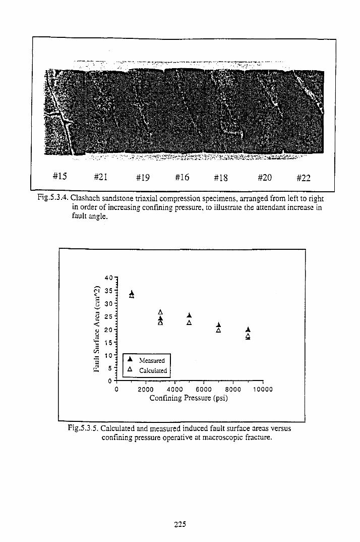
#15 #21 #19 #16 #18 #20 #22

Fig.5.3.4. Clashach sandstone triaxial compression specimens, arranged from left to right in order of increasing confining pressure, to illustrate the attendant increase in fault angle.

Cl

40

35<o 30

p 25<<u 20o

15c/5

1 0

r»* 5

0

è

Aà

AA A

A

— I--------- 1--------1-------- ----------1------------------ 1—

2000 4000 6000 8000Confining Pressure (psi)

A4

— i10000

Fig.5.3.5. Calculated and measured induced fault surface areas versus confining pressure operative at macroscopic fracture.

225

and strength enhanced recovery stress states. Each was recorded under constant stress

conditions achieved through servo-control of the confining pressure and by holding the

axial load constant under displacem ent control. The perm eability equipment

configuration, experimental method and underlying physics are as outlined in section

4.3.1. Each Clashach core plug was tested under “drained” triaxial conditions, that is

with an external pressure source connected continuously to the pore system of the rock

with the aim of maintaining constancy of pore pressure by introducing or removing fluid.

In the Clashach sandstone test programme the downstream end of each core plug was left

open to the atmosphere, so that pore pressure was equivalent to a constant atmospheric

pressure. Such drained conditions (rock specimen in continuous contact with the pore

fluid reservoir, with permeability being sufficient to enable pore pressure to remain

constant and uniform even on specimen deformation) are in direct contrast to

“undrained” conditions, in which the specimen is saturated and then isolated from the

pore fluid reservoir, so that changes in pore pressure will be induced by changes in

porosity accompanying deformation. As noted in section 4.3.1, a metering pump was

used to apply a pressure pulse of about 30psi to the upstream end of the core, at a

constant flow rate equivalent to 0.15ccs_1. Transient pressure pulse decay across the

sample was measured using a differential pressure transducer, whilst an x-y-t chart

recorder provided simultaneous hardcopy of the Ap-time curve. Numerical integration of

the pressure decay curve over the appropriate real time interval is achieved without

defining its explicit function, by measuring the area under the hardcopy curve using a

digital planim eter. The system com pressibility constant, C, was determined

experimentally to be 2.59 x 10_11 m 3Pa4, by measuring pressure change associated with

injecting known volumes of permeant into the upstream reservoir. It should be noted that

the value of C is dependent on the permeant used. Viscosity of the pore fluid, a refined

mineral oil (Shell Tellus 15) was measured at room temperature, using a Brookfield

dynamic viscometer, at 18 x 10'3Pasecs (18cP). Specimen lengths and cross-sectional

areas were measured using digital callipers, however only change in length was corrected

on specimen deformation.

226

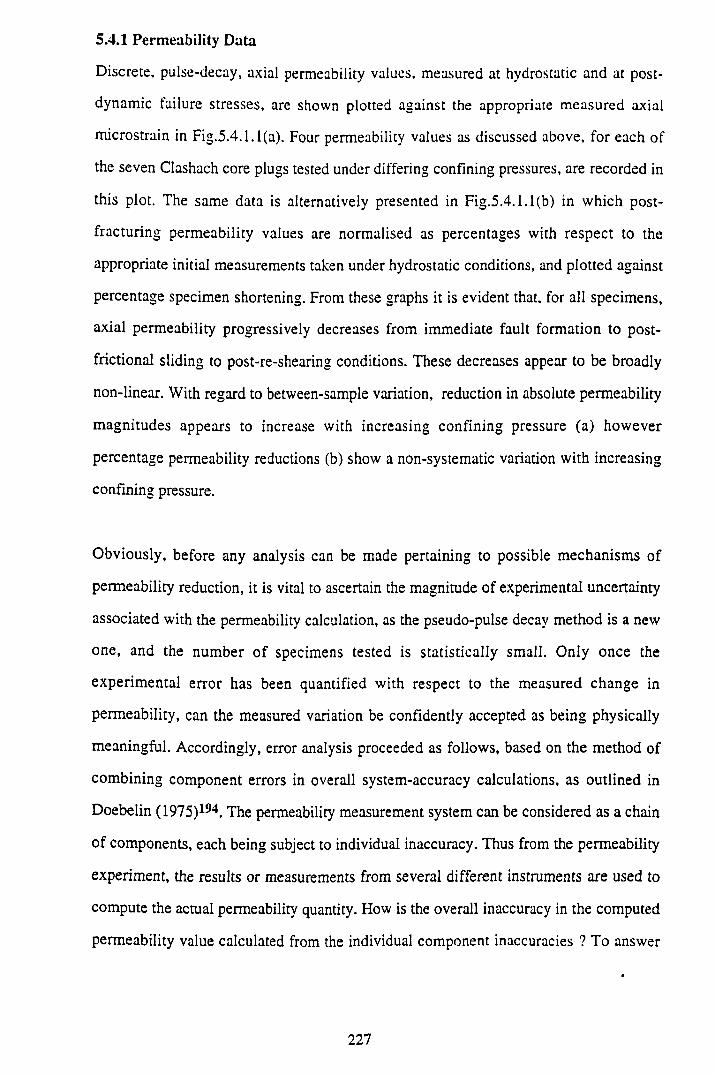
5.4.1 Perm eability Data

Discrete, pulse-decay, axial permeability values, measured at hydrostatic and at post­

dynamic failure stresses, are shown plotted against the appropriate measured axial

microstrain in Fig.5.4.1.1(a). Four permeability values as discussed above, for each of

the seven Clashach core plugs tested under differing confining pressures, are recorded in

this plot. The same data is alternatively presented in Fig.5.4 .1.1(b) in which post­

fracturing permeability values are normalised as percentages with respect to the

appropriate initial measurements taken under hydrostatic conditions, and plotted against

percentage specimen shortening. From these graphs it is evident that, for all specimens,

axial permeability progressively decreases from immediate fault formation to post-

frictional sliding to post-re-shearing conditions. These decreases appear to be broadly

non-linear. With regard to between-sample variation, reduction in absolute permeability

magnitudes appears to increase with increasing confining pressure (a) however

percentage permeability reductions (b) show a non-systematic variation with increasing

confining pressure.

Obviously, before any analysis can be made pertaining to possible mechanisms of

permeability reduction, it is vital to ascertain the magnitude of experimental uncertainty

associated with the permeability calculation, as the pseudo-pulse decay method is a new

one, and the number o f specimens tested is statistically small. Only once the

experim ental error has been quantified with respect to the measured change in

permeability, can the measured variation be confidently accepted as being physically

meaningful. Accordingly, error analysis proceeded as follows, based on the method of

combining component errors in overall system-accuracy calculations, as outlined in

Doebelin (1975)194. The permeability measurement system can be considered as a chain

of components, each being subject to individual inaccuracy. Thus from the permeability

experiment, the results or measurements from several different instruments are used to

compute the actual permeability quantity. How is the overall inaccuracy in the computed

permeability value calculated from the individual component inaccuracies ? To answer

227

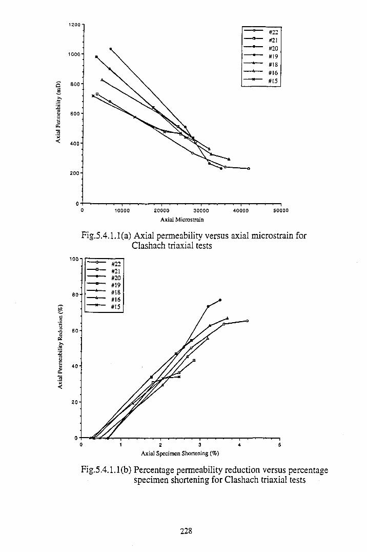
Axia

l Per

mea

bilit

y Re

duct

ion

(%)

Axia

l Per

mea

bilit

y (m

D)

F ig .5 .4 .1 .1 (a ) A x ia l perm eability versus axial m icrostrain for C lashach triaxial tests

F ig .5 .4 .1 .1 (b ) Percentage perm eability reduction versus percentage specim en shortening for C lashach triaxial tests

228

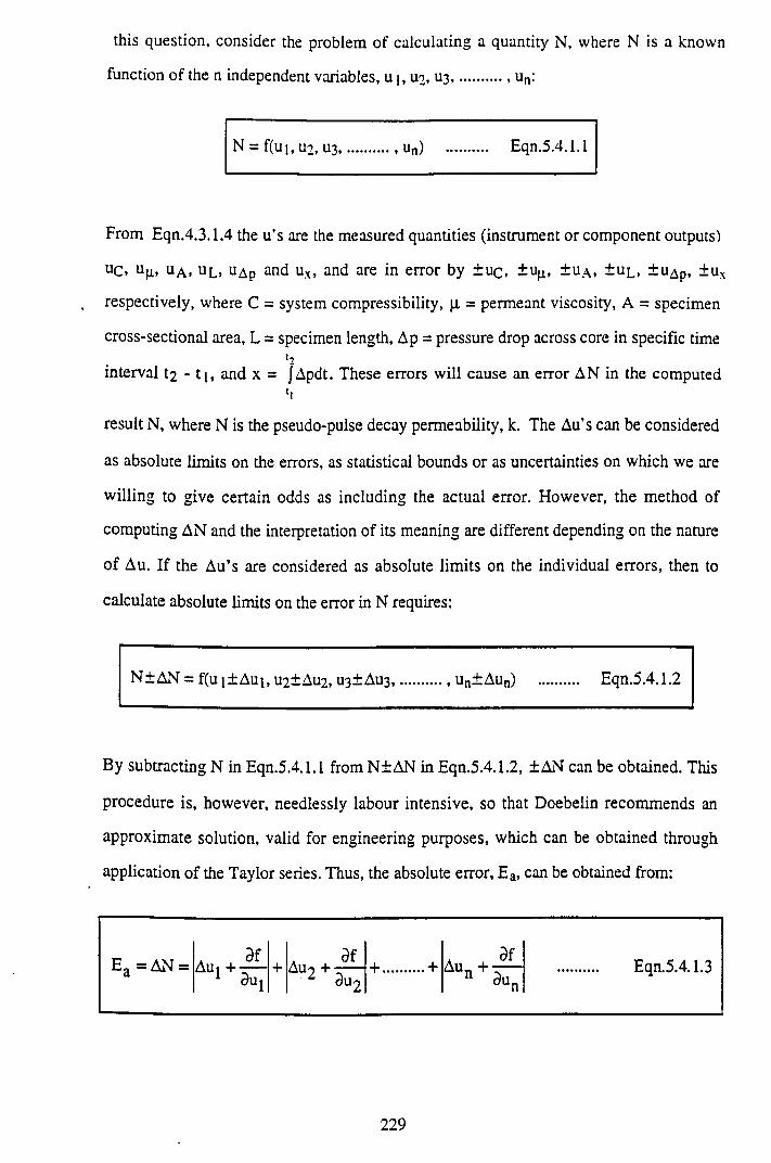
this question, consider the problem of calculating a quantity N, where N is a known

function of the n independent variables, u i, U2, U3, .......... , un:

N = f(uj, U2, U3.............. un) ............ Eqn.5.4.1.1

From Eqn.4.3.1.4 the u’s are the measured quantities (instrument or component outputs)

UC. Uji, ua , ul, uap and ux, and are in error by ±uc, tu^, ± ua, ± ul, ± uap, ± ux

respectively, where C = system compressibility, |i = permeant viscosity, A = specimen

cross-sectional area, L = specimen length, Ap = pressure drop across core in specific time*2

interval t2 - 11, and x = jApdt. These errors will cause an error AN in the computed‘i

result N, where N is the pseudo-pulse decay permeability, k. The Au’s can be considered

as absolute limits on the errors, as statistical bounds or as uncertainties on which we are

willing to give certain odds as including the actual error. However, the method of

computing AN and the interpretation of its meaning are different depending on the nature

o f Au. If the Au’s are considered as absolute limits on the individual errors, then to

calculate absolute limits on the error in N requires:

N±AN = f(ui±A ui,U 2±Au2, U3±Au3, ............ un±Aun) ........... Eqn.5.4.1.2

By subtracting N in Eqn.5.4.1.1 from N±AN in Eqn.5.4.1.2, ±AN can be obtained. This

procedure is, however, needlessly labour intensive, so that Doebelin recommends an

approximate solution, valid for engineering purposes, which can be obtained through

application of the Taylor series. Thus, the absolute error, E a, can be obtained from:

Ea = AN = * df 3f A 9fAU1++i u ^

+ ..........+Au" X

Eqn.5.4.1.3

229

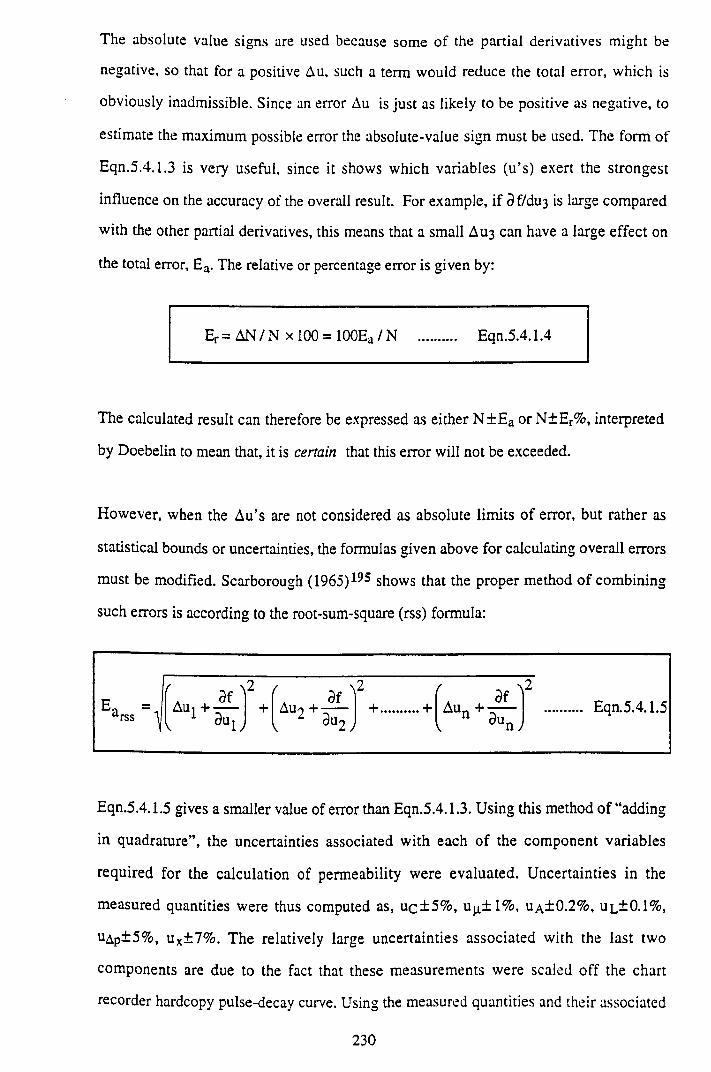
The absolute value signs are used because some of the partial derivatives might be

negative, so that for a positive Au, such a term would reduce the total error, which is

obviously inadmissible. Since an error Au is just as likely to be positive as negative, to

estimate the maximum possible error the absolute-value sign must be used. The form of

Eqn.5.4.1.3 is very useful, since it shows which variables (u’s) exert the strongest

influence on the accuracy of the overall result. For example, if 3 f/du3 is large compared

with the other partial derivatives, this means that a small AU3 can have a large effect on

the total error, Ea. The relative or percentage error is given by:

Er = AN / N x 100 = 100Ea / N .......... Eqn.5.4.1.4

The calculated result can therefore be expressed as either N ± E a or N ±Er%, interpreted

by Doebelin to mean that, it is certain that this error will not be exceeded.

However, when the Au’s are not considered as absolute limits of error, but rather as

statistical bounds or uncertainties, the formulas given above for calculating overall errors

must be modified. Scarborough (1965)195 shows that the proper method of combining

such errors is according to the root-sum-square (rss) formula:

Eqn.5.4.1.5 gives a smaller value of error than Eqn.5.4.1.3. Using this method of “adding

in quadrature”, the uncertainties associated with each o f the component variables

required for the calculation of permeability were evaluated. Uncertainties in the

measured quantities were thus computed as, u c± 5 % , u^+1% , ua±0.2%, ul±0.1%,

UAp±5%, u x±7% . The relatively large uncertainties associated with the last two

components are due to the fact that these measurements were scaled off the chart

recorder hardcopy pulse-decay curve. Using the measured quantities and their associated

230

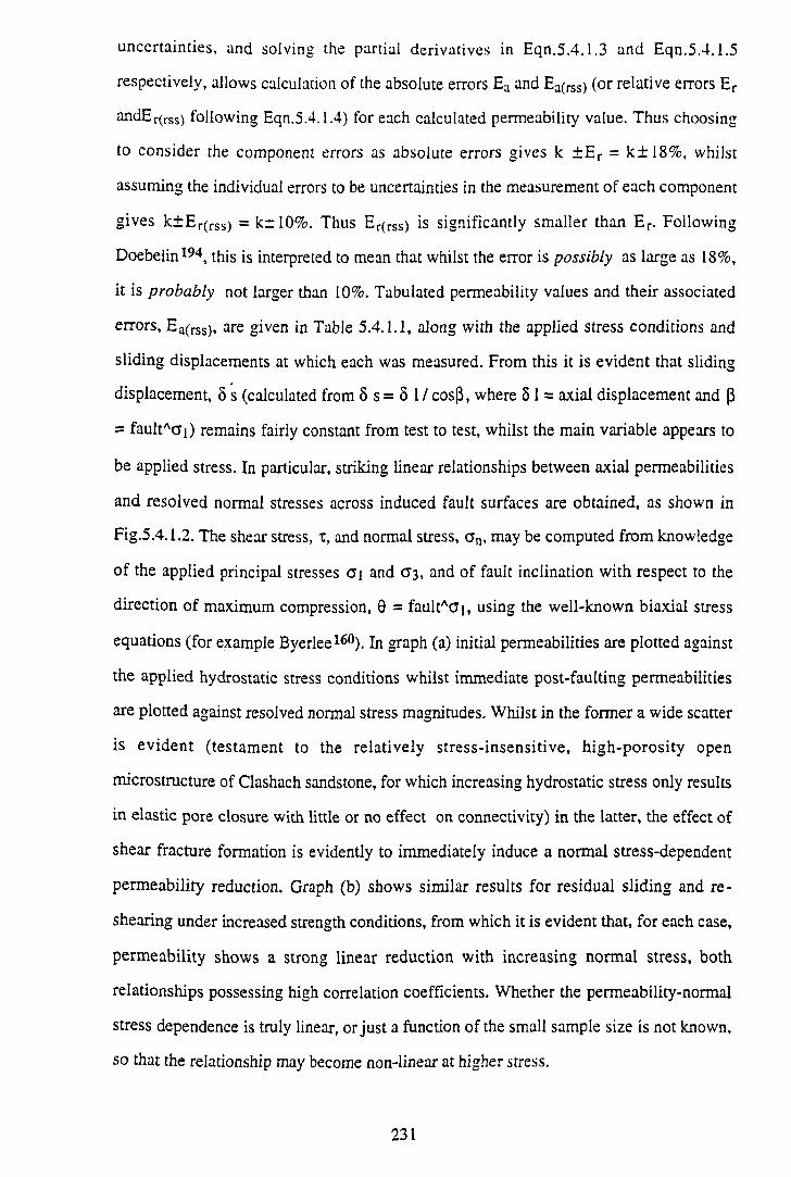
uncertainties, and solving the partial derivatives in Eqn.5.4.1.3 and Eqn.5.4.1.5

respectively, allows calculation of the absolute errors Ea and Ea(rss) (°r relative errors E r

andEr(rss) following Eqn.5.4.1.4) for each calculated permeability value. Thus choosing

to consider the component errors as absolute errors gives k ± E r = k±18% , whilst

assuming the individual errors to be uncertainties in the measurement of each component

gives k ± E r(rss) = k±10%. Thus E r(rsS) is significantly smaller than E r. Following

Doebelin194, this is interpreted to mean that whilst the error is possibly as large as 18%,

it is probably not larger than 10%. Tabulated permeability values and their associated

errors, E a(rss), are given in Table 5.4.1.1, along with the applied stress conditions and

sliding displacements at which each was measured. From this it is evident that sliding

displacement, 8 s (calculated from 5 s = 8 1 / cos(J, where 81 = axial displacement and (5

= faultACi) remains fairly constant from test to test, whilst the main variable appears to

be applied stress. In particular, striking linear relationships between axial permeabilities

and resolved normal stresses across induced fault surfaces are obtained, as shown in

Fig.5.4.1.2. The shear stress, t , and normal stress, a n, may be computed from knowledge

of the applied principal stresses a t and a 3, and of fault inclination with respect to the

direction o f maximum compression, 9 = faultAOi, using the well-known biaxial stress

equations (for example Byerlee160). In graph (a) initial permeabilities are plotted against

the applied hydrostatic stress conditions whilst immediate post-faulting permeabilities

are plotted against resolved normal stress magnitudes. Whilst in the former a wide scatter

is evident (testam ent to the relatively stress-insensitive, high-porosity open

microstructure of Clashach sandstone, for which increasing hydrostatic stress only results

in elastic pore closure with little or no effect on connectivity) in the latter, the effect of

shear fracture formation is evidently to immediately induce a normal stress-dependent

permeability reduction. Graph (b) shows similar results for residual sliding and re­

shearing under increased strength conditions, from which it is evident that, for each case,

permeability shows a strong linear reduction with increasing normal stress, both

relationships possessing high correlation coefficients. Whether the permeability-normal

stress dependence is truly linear, or just a function of the small sample size is not known,

so that the relationship may become non-linear at higher stress.

231

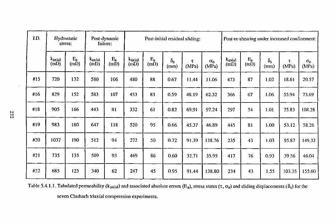
232

ID . Hydrostaticstress:

Post-dynamicfailure:

Post-initial residual sliding: Post-re-shearing under increased confinement:

kaxial(mD)

Ea(mD)

kaxial(mD)

Ea(mD)

kaxial(mD)

Ea(mD) 5s

(mm)x

(MPa)On

(MPa)kaxial(mD)

Ea(mD) 5s

(mm)X

(MPa)o n

(MPa)

#15 720 132 580 106 480 88 0.67 11.44 11.06 473 87 1.02 18.61 20.57

#16 829 152 583 107 453 83 0.59 48.19 62.32 366 67 1.06 55.94 73.69

#18 905 166 443 81 332 61 0.82 69.91 97.24 297 54 1.01 75.83 108.28

#19 983 180 647 118 520 95 0.66 45.37 46.89 445 81 1.00 53.12 58.26

#20 1037 190 512 94 272 50 0.72 91.39 138.76 235 43 1.03 95.87 149.32

#21 735 135 509 93 469 86 0.60 32.71 35.95 417 76 0.93 39.56 46.04

#22 685 125 340 62 247 45 0.95 91.44 138.80 234 43 1.55 103.35 155.60

Table 5.4.1.1. Tabulated permeability (kaxjai) and associated absolute errors (Ea), stress states (x, o n) and sliding displacements (8S) for the

seven Clashach triaxial compression experiments.

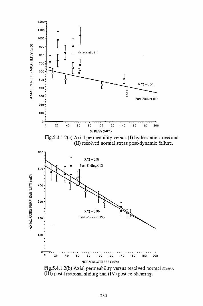
AX

IAL

CORE

PER

MEA

BILI

TY (m

D)

AXIA

L CO

RE P

ERM

EABI

LITY

(raD

)

1200 n

100 ■

0 ..... ...................| i i . i | i i i i | , , , , | . i i i | i ................................. i i < -i | i ■ i ■ | < i i ................ ................................ ................................

0 20 40 60 80 100 120 140 160 180 200

STRESS (MPa)

Fig.5.4 .1.2(a) Axial permeability versus (I) hydrostatic stress and (II) resolved normal stress post-dynamic failure.

Fig.5.4.1.2(b) Axial permeability versus resolved normal stress (III) post-frictional sliding and (IV) post-re-shearing.

233

It is evident, however, that the effect of increased frictional sliding (post-dynamic failure

with little or no shear displacement, to frictional sliding, to re-shearing conditions) in this

test programme has been to progressively reduce permeability. Further, it is inferred that

the associated generation of frictional wear debris (fault gouge) from the displaced

fracture walls, has produced a granular shear band (in many respects morphologically

similar to a natural granulation seam) oblique to the direction of fluid flow, which under

increased stress (and being particularly susceptible to normal stress acting perpendicular

to the fracture zone) has provided a normal stress-sensitive granular baffle responsible

for the observed decrease in axial permeability measurements. In Chapter 6 , this

relationship will be further examined through particle-size analysis of the collected fault

gouge samples, whilst in the discussion below, the potential of variable fault inclination

to influence axial permeability measurements is also assessed.

5.4.2 Discussion

As noted in section 5.3, due to the non-linear failure envelope appropriate to Clashach

sandstone, the angle 9 = faultAa i shows a steady increase with increasing C3. One

important consequence of such a stress-dependent fault inclination already mentioned, is

that induced fault area subsequently decreases in a remarkably linear fashion as 03

increases (Fig.5.3.5). Were the failure envelope truly linear as in the conventional

Coulomb sense, then observed changes in axial permeability could positively be ascribed

to either differences in applied stress, resultant slip displacements or microstructural

alteration (or combinations o f all three). However, this disparity in fracture

inclination/elliptical area between test specimens in effect represents yet another test

variable with the potential to have a systematic influence on axial permeability

measurements over the core lengths. It is thus desirable to conduct a semi-quantitative

analysis of the relative control that such a variation in fracture area might have on fluid

flow, before commenting on permeability variation as a direct function o f gouge

evolution.

234

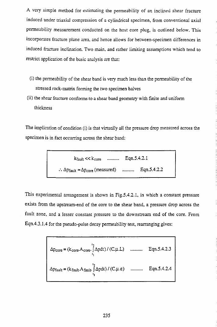
A very simple method for estimating the permeability of an inclined shear fracture

induced under triaxial compression of a cylindrical specimen, from conventional axial

permeability measurement conducted on the host core plug, is outlined below. This

incorporates fracture plane area, and hence allows for between-specimen differences in

induced fracture inclination. Two main, and rather limiting assumptions which tend to

restrict application of the basic analysis are that:

(i) the permeability of the shear band is very much less than the permeability of the

stressed rock-matrix forming the two specimen halves

(ii) the shear fracture conforms to a shear band geometry with finite and uniform

thickness

The implication of condition (i) is that virtually all the pressure drop measured across the

specimen is in fact occurring across the shear band:

kfault« kcore .......... Eqn.5.4.2.1

Apfauit = Apcore (measured) .......... Eqn.5.4.2.2

This experimental arrangement is shown in Fig.5.4.2.1, in which a constant pressure

exists from the upstream-end of the core to the shear band, a pressure drop across the

fault zone, and a lesser constant pressure to the downstream end of the core. From

Eqn.4.3.1.4 for the pseudo-pulse decay permeability test, rearranging gives:

‘2Apcore = (^core-A-core- } Apdt) / (C.JI.L) ..... .... Eqn.5.4.2.3

Apfauit= (kfault-Afault* J Apdt) / (C.[i.£) ..... .... Eqn.5.4.2.4

235

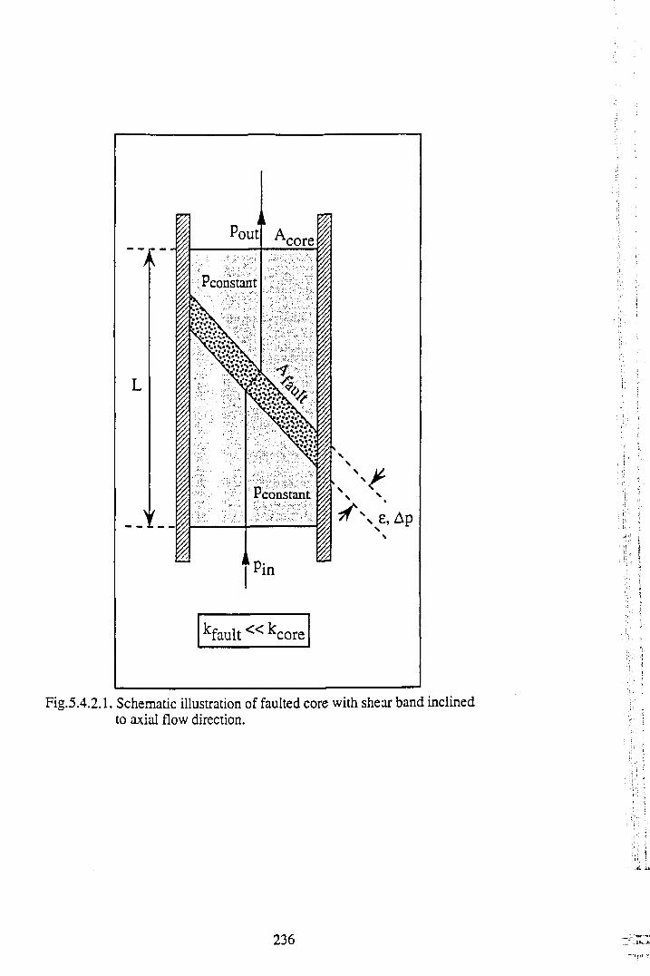
Fig.5.4.2.1. Schematic illustration of faulted core with shear band inclined to axial flow direction.

236

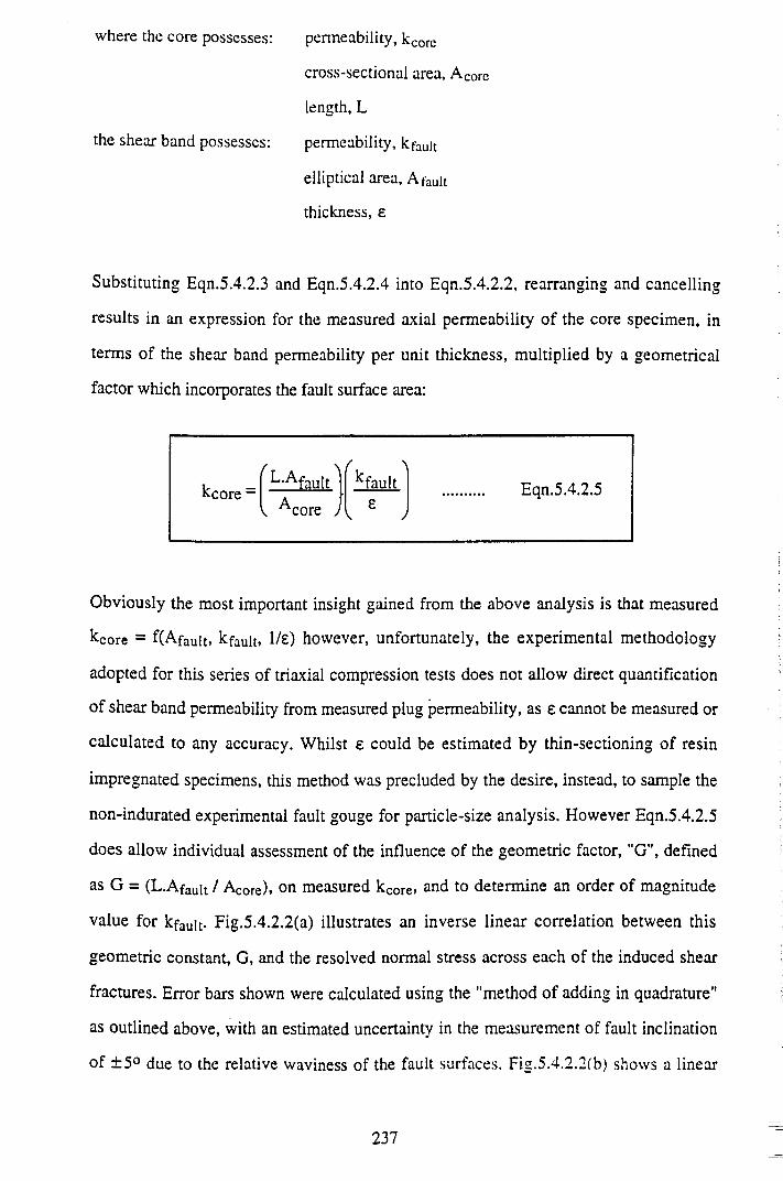
where the core possesses: permeability, kcorc

cross-sectional area, A COre

length, L

the shear band possesses: permeability, kfau|t

elliptical area, A fauit

thickness, £

Substituting Eqn.5.4.2.3 and Eqn.5.4.2.4 into Eqn.5.4.2.2, rearranging and cancelling

results in an expression for the measured axial permeability of the core specimen, in

terms of the shear band permeability per unit thickness, multiplied by a geometrical

factor which incorporates the fault surface area:

kcore -/ T A

L-AfaultA

Kfault .......... Eqn.5.4.2.5 r tcore 7 £

\ )

Obviously the most important insight gained from the above analysis is that measured

kcore = f(Afauit, kfault. 1/e) however, unfortunately, the experimental methodology

adopted for this series of triaxial compression tests does not allow direct quantification

of shear band permeability from measured plug permeability, as £ cannot be measured or

calculated to any accuracy. Whilst £ could be estimated by thin-sectioning of resin

impregnated specimens, this method was precluded by the desire, instead, to sample the

non-indurated experimental fault gouge for particle-size analysis. However Eqn.5.4.2.5

does allow individual assessment of the influence of the geometric factor, "G", defined

as G = (L.Afauit / Acore). cm measured kCOre. and to determine an order of magnitude

value for kfaujt. Fig.5.4.2.2(a) illustrates an inverse linear correlation between this

geometric constant, G, and the resolved normal stress across each of the induced shear

fractures. Error bars shown were calculated using the "method of adding in quadrature"

as outlined above, with an estimated uncertainty in the measurement of fault inclination

of ± 5° due to the relative waviness of the fault surfaces. Fig.5.4.2.2(b) shows a linear

237

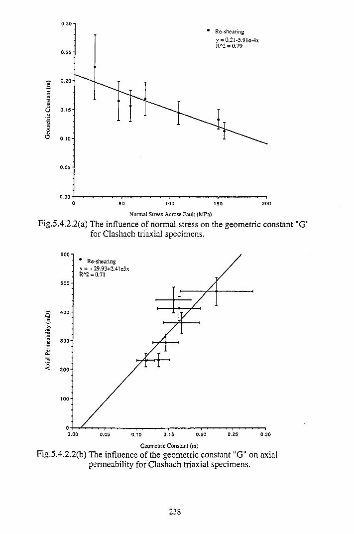
0 .30 -1

0.05-

o.oo H— i— i— i— >—t— ■ ' ■ ■ "11— ...................— i— ■— ■ » ' l l0 50 100 150 200

Normal Stress Across Fault (MPa)

Fig.5.4.2.2(a) The influence of normal stress on the geometric constant "G" for Clashach triaxial specimens.

Geometric Constant (m)

Fig.5.4.2.2(b) The influence of the geometric constant "G" on axial permeability for Clashach triaxial specimens.

238

relationship between the measured axial permeability, kcorc* und the geometric constant,

G. These empirically determined variations, G «= l / a n and kcore G, suggest that the

observed inverse linear correlation’s between measured axial plug permeabilities and

resolved normal stress across the induced faults (see Fig.5.4.1.2) kcore «= <7n, are

influenced by variable fault plane inclination, imparting a stress-dependency to the

geometric constant, G. Thus it is apparent that the effect of a non-linear failure envelope

on 9 = faultAa i is being reflected in the measured k COre- However, the lower correlation

coefficient for the normal stress-dependency of G (R2 = 0.79) compared with that for

kcore (R2 = 0.96) does suggest that an additional structural contribution to the axial

permeability stress-sensitivity, perhaps due to fault gouge, also exists.

In the above analysis, only data relating to the process of re-shearing has been discussed,

however it is believed that the same principle (that is the dependency of kCOre on G) will

also apply to post-dynamic failure and residual sliding conditions. The main difference

between calculated G-values for these different conditions will lie in estimation of Afauit,

which strictly speaking will vary with sliding displacement (similar to that given in

section 3.4.3 for sliding circles, but for the contact area of overlapping ellipses with

displaced centres). However, as the ratio of sliding displacement to semi-major axes

length varies in the range of 1 to 3% for the triaxial compression specimens, this minor

correction has been ignored, with Afauit being taken simply as that calculated from fault

inclination, with no shear displacement correction. In Chapter 6 , using plausible

predictions of fault thickness (e) variation with increasing confining pressure, estimates

are made of kfauit for all seven specimens, and relationships explored between these

values and resolved normal stress across the shear bands, variation in angular shear strain

resulting from thickness and slip displacement differences, and variance between certain

sampled fault gouge particle size distribution parameters.

5.5 M ICROSEISM IC RESULTS

In this final section, acoustic emission data complimenting the strength and permeability

results outlined above, will be reviewed. Prior to this, and in order to aid in digestion of

239

the AE results and their implications, brief summaries of both fractal set and damage

mechanics theories are given in sections 5.5.1 and 5.5.2 respectively. Differential stress

and natural AE were measured over three separate phases corresponding to fault

nucleation (phase I), frictional sliding (phase II) and fault strengthening (re-shearing

under increased confinement, phase III). The AE was interpreted using a mean field

theory for damage evolution, in terms of temporal variation in seismic event rate, b-value

and the inferred fractal dimension of the AE. Whilst results from the fault nucleation

phase confirm other observations of damage evolution leading to failure reported in the

literature (see below for pertinent references) AE monitoring for the frictional sliding

stages II and III under triaxial compression, and subsequent interpretation of the

collected data, represents new work which offers important insights into the physical

processes involved. Prior to this study, the only reported incidence of AE monitoring

during shearing of rock discontinuities, was that of Li & Nordlund (1990)196 who

reported characteristics of AE resulting from frictional sliding, of both artificial and

natural sliding surfaces in granite and slate samples, under direct shear (unconfined,

constant normal stress) conditions. Their test results indicated that the AE rate peaks

coincided with the stress drops caused by fracturing of asperities during shear. When the

discontinuity surface became smooth, the strength reached a residual value, the shear

stress drops became larger and less frequent, and the AE count rate declined. The AE

intensity was seen to depend on both the roughness and the compressive strength of the

discontinuity surface. Ideally, perhaps what is required is a combination of the fractal

damage mechanics theory used to evaluate the triaxial compression AE data recorded

during this present study, with the experimental advantages of large fault surface area,

known boundary conditions and significant slip displacements common to the direct

shear method of Li & Nordlund.

5-5.1 Definition of a Fractal Set

Prior to a discussion of acoustic emission statistics and also before considering measured

fault gouge distributions, it is considered pertinent to provide a brief outline of some of

the more essential features underlying the theory of fractals. Mandelbrot (1967)197

240

introduced the concept of fractals. With regard to derivation of the term he noted that, “I

coined the term “fractal” from the latin fractus which describes the geometry of a

broken stone.” The adjective “fractus” means irregular or broken. M andelbrot

introduced fractals within the context of scale invariance. The scale invariance of

geological phenomena is easily understood when consideration is given to the fact that,

without the inclusion of a suitable object of known dimensions to define the scale of

observation, such as a hammer a coin or a person, it is often impossible to determine

whether a photograph of a geological feature covers a scale appropriate to a thin-section

or to a cliff face (mm’s or km’s). Without inclusion of an object with a characteristic

dimension, the scale of the photograph cannot be determined. With recourse to the now

classic example of the length of a rocky coastline obtained using a measuring rod with a

specified length, due to scale invariance the length of the coastline increases as the length

of the measuring rod decreases according to a power law. The power exponent

determines the fractal dimension of the coastline, and it is noted that it is not possible to

obtain a specific or unique value for the length of the coastline, owing to all the minor

indentations down to a scale of mm’s or less. Many phenomena relating to shear

fracturing are scale invariant, including the frequency-size distributions of acoustic

emissions, faults, earthquakes and shear debris (gouge). Thus the fractal dimension

provides a powerful tool for describing scale invariant geometries. A fractal distribution

requires that the number of objects larger than a specified size has a power-law

dependence on the size. However, the empirical applicability of power-law statistics to

geological phenomena was recognised long before the concept of fractals was conceived,

an example being the Gutenberg-Richter relation for the frequency-magnitude statistics

of earthquakes (Gutenberg & Richter, 1954)198. Power-laws are of course not the only

statistical distributions to be applied to geological processes, other examples being the

normal and log-normal distributions, although the power law is the only one not to

include a characteristic length scale. Thus the power-law distribution must be applicable

to scale-invariant phenomena. Whilst scale-invariance provides a rational basis for the

applicability of the power law, fractal distribution, fractal concepts can also be applied to

continuous distributions, an example being topography, where the fractal dimension is a

241

measure of the roughness of the features. Thus fractals are also capable of uniquely

describing fault (or joint) surface morphologies for comparative purposes relating to

strength and fluid flow studies. In the following section a definition of a fractal set is

given, after Turcotte (1992)199 pages 6-17.

Following Turcotte consider the definition of a fractal set according to:

Nn = C/rnD .......... Eqn.5.5.1.1

where N n is the number of objects (fragments) with a characteristic linear dimension rn,

C is a constant of proportionality and D is the fractal dimension. The fractal dimension

can be an integer, in which case it is equivalent to a Euclidian dimension. The Euclidian

dimension of a point is zero, of a line segment is one, of a square is two and of a cube is

three. In general the fractal dimension is not an integer, but a fractional dimension. This

is the origin of the term fractal, and its application to irregular (non-Euclidian) geometry

is encapsulated in its derivation.

To illustrate why it is appropriate to refer to D as a fractional dimension, consider the

line segment shown in Fig.5.5.1.1 (a) which is divided into two parts so that r i = 1/2 and

one part retained so that N i = 1. The remaining segment is then divided into two pans so

that r2 = 1/4 and again one segment retained so that N 2 = I. In order to determine D,

Eqn.5.5.1.1 can be rewritten in terms of logarithms to the base e as:

D = In(Nn+i / N n) / In(rn / rn+i ) .......... Eqn.5.5.1.2

Thus for the example considered, In(N2/N 1) = In i = 0, In(r i/r2) = In2, and D = 0, the

Euclidian dimension of a point. With reference to the examples (b) to (f) also shown in

Fig.5.5.1.1: (b) a line segment is divided into three parts and one retained, D = Inl/In3 =

0, the fractal dimension of a point; (c) a line segment is divided into two parts and both

242

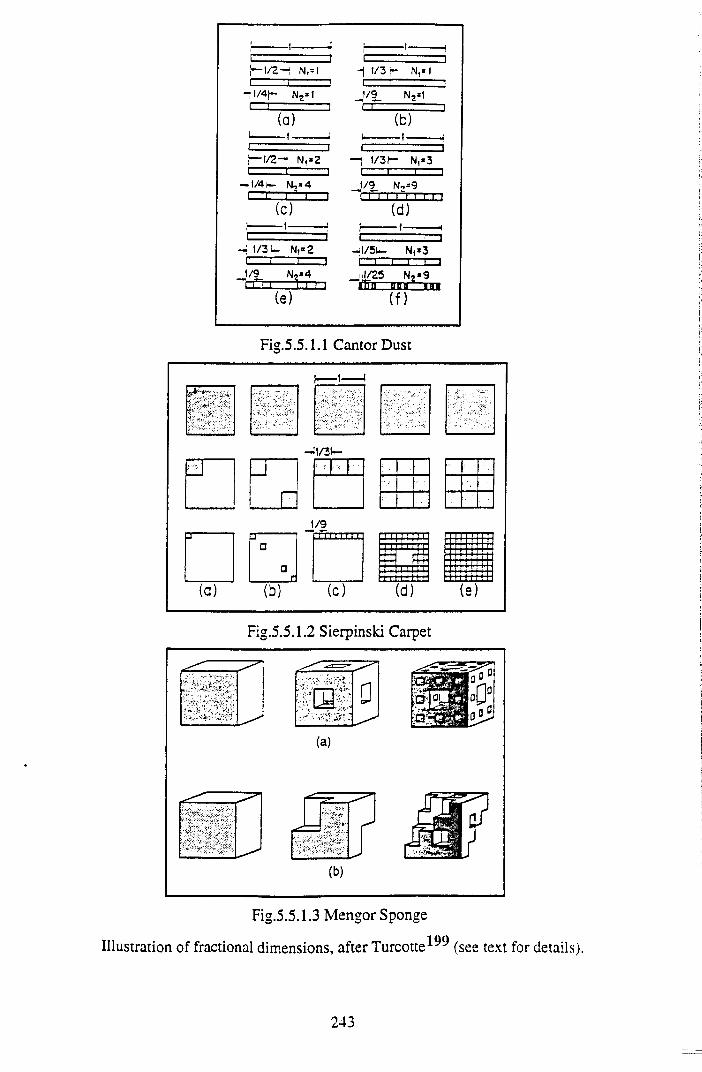
I"'" -----11— 1/2—í N,= 1 I" I !

-¡1/4f- N2»l

(a)!-------1--------1i 'i1— 1/2~i N,»2

—í 1/4-1— N ,*4r~~r i ' i

(0I------- 1-------JI I

- i 1/3 i - N,*2 CTZI'—" I = 3 1/9 N2*4

(e)

-j 1/3 j- N,* 1

J/9_ N2=1~i '

(b)i------- 1—

-1 1/31- N,*3l i l i1/9 N,=9

l-i r n ~i i m(d)

i-------1--------1CZ" , —]

mWSU- N,*3I!. I"~"l I I *~1

jli/25 N2«9aHn~iiBa _m

(f)

Fig.5.5.1.1 Cantor Dust

(b)

Fig.5.5.1.3 Mengor Sponge

Illustration of fractional dimensions, after T u r c o t te ^ (See text for details).

243

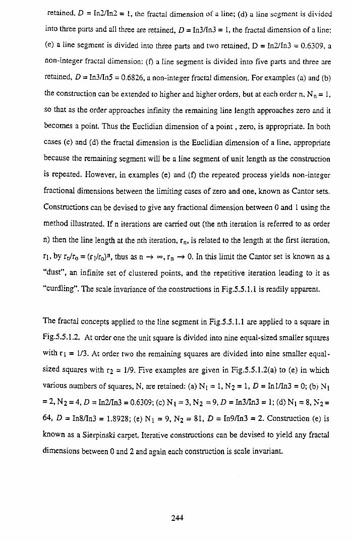
retained, D = In2/In2 = 1, the fractal dimension of a line; (d) a line segment is divided

into three parts and all three are retained, D = In3/ln3 = 1, the fractal dimension of a line;

(e) a line segment is divided into three parts and two retained, D = In2/In3 = 0.6309, a

non-integer fractal dimension: (f) a line segment is divided into five parts and three are

retained, D = In3/In5 = 0.6826, a non-integer fractal dimension. For examples (a) and (b)

the construction can be extended to higher and higher orders, but at each order n, N n = 1,

so that as the order approaches infinity the remaining line length approaches zero and it

becomes a point. Thus the Euclidian dimension of a p o in t, zero, is appropriate. In both

cases (c) and (d) the fractal dimension is the Euclidian dimension of a line, appropriate

because the remaining segment will be a line segment of unit length as the construction

is repeated. However, in examples (e) and (f) the repeated process yields non-integer

fractional dimensions between the limiting cases of zero and one, known as Cantor sets.

Constructions can be devised to give any fractional dimension between 0 and 1 using the

method illustrated. If n iterations are carried out (the nth iteration is referred to as order

n) then the line length at the nth iteration, r n, is related to the length at the first iteration,

r l, by rn/r0 = (r i/r0)n, thus as n r n 0. In this limit the Cantor set is known as a

“dust”, an infinite set of clustered points, and the repetitive iteration leading to it as

“curdling”. The scale invariance of the constructions in Fig.5.5.1.1 is readily apparent.

The fractal concepts applied to the line segment in Fig.5.5.1.1 are applied to a square in

Fig.5.5.1.2. At order one the unit square is divided into nine equal-sized smaller squares

with r i = 1/3. At order two the remaining squares are divided into nine smaller equal-

sized squares with r2 = 1/9. Five examples are given in Fig.5.5.1.2(a) to (e) in which

various numbers of squares, N, are retained: (a )N i = l ,N 2 = l f £ = Inl/In3 = 0; (b) Nj

= 2, N 2 = 4, D = In2/In3 = 0.6309; (c) N i = 3, N 2 = 9, D = In3/In3 = 1; (d) Ni = 8, N2 =

64, D = In8/In3 = 1.8928; (e) N i = 9, N2 = 81, D = In9/In3 = 2. Construction (e) is

known as a Sierpinski carpet. Iterative constructions can be devised to yield any fractal

dimensions between 0 and 2 and again each construction is scale invariant.

244

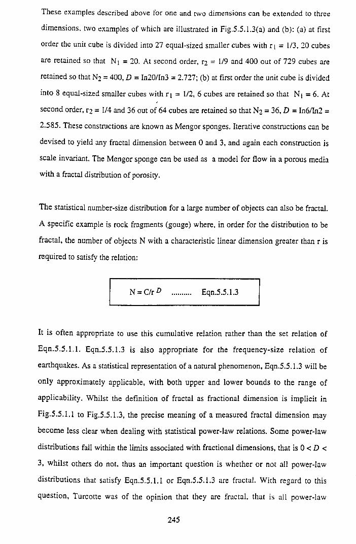
These examples described above for one and two dimensions can be extended to three

dimensions, two examples of which are illustrated in Fig.5.5 .1.3(a) and (b): (a) at first

order the unit cube is divided into 27 equal-sized smaller cubes with r i = 1/3, 20 cubes

are retained so that Nj = 2 0 . At second order, r2 = 1/9 and 400 out of 729 cubes are

retained so that N2 = 400, D = In20/In3 = 2.727; (b) at first order the unit cube is divided

into 8 equal-sized smaller cubes with r i = 1/2, 6 cubes are retained so that N | = 6. At

second order, r 2 = 1/4 and 36 out of 64 cubes are retained so that N2 = 36, D = In6/In2 =

2.585. These constructions are known as Mengor sponges. Iterative constructions can be

devised to yield any fractal dimension between 0 and 3, and again each construction is

scale invariant. The Mengor sponge can be used as a model for flow in a porous media

with a fractal distribution of porosity.

The statistical number-size distribution for a large number of objects can also be fractal.

A specific example is rock fragments (gouge) where, in order for the distribution to be

fractal, the number of objects N with a characteristic linear dimension greater than r is

required to satisfy the relation:

N = C/r ^ .......... Eqn.5.5.1.3

It is often appropriate to use this cumulative relation rather than the set relation of

Eqn.5.5.1.1. Eqn.5.5.1.3 is also appropriate for the frequency-size relation of

earthquakes. As a statistical representation of a natural phenomenon, Eqn.5.5.1.3 will be

only approximately applicable, with both upper and lower bounds to the range of

applicability. Whilst the definition of fractal as fractional dimension is implicit in

Fig.5.5.1.1 to Fig.5.5.1.3, the precise meaning of a measured fractal dimension may

become less clear when dealing with statistical power-law relations. Some power-law

distributions fall within the limits associated with fractional dimensions, that is 0 < D <

3, whilst others do not, thus an important question is whether or not all power-law

distributions that satisfy Eqn.5.5.1.1 or Eqn.5.5.1.3 are fractal. With regard to this

question, Turcotte was of the opinion that they are fractal, that is all power-law

245

distributions fulfilling these criteria, but with D -values outwith the fractional dimension

range, should be considered fractal, noting that, “such distributions are clearly scale

invariant even if not directly associated with a fractal dimension.”

5.5.2 Fractal Damage Mechanics

The concept of a single variable, or set of variables, used to describe the changing state

of the microstructure of a material as it is deformed, is referred to as a damage theory.

There are three basic elements to any damage theory: a definition of damage; an

evolutionary equation for the damage; a constitutive equation relating the strains to the

stresses and the damage. A simple damage theory for the uniaxial tensile loading of a

brittle material is outlined by Costin181 pages 196-198, and is cited as a simple example

prior to discussion of the more complex problem of failure under compressional loading.

Main et al (1993)200 proposed an idealised synoptic model of damage development in a

heterogeneous brittle solid under compression. In it, test specimens or in situ “elements”

of rock are considered to fail under compressional loading ultimately by the organised,

unstable coalescence of microcracks which initially grow in tensile mode, nucleating

first on the weakest elements in a polycrystalline matrix. Initially crack growth is stable

and distributed throughout the sample, implying that the sites o f incremental crack

growth initially tend to avoid one another, testament to a kind of negative feedback

process operating on the microscopic level. Thus crack growth is initially energetically

favourable, but only for a small increment until the energy balance favours arrest or

rupture. In the early stages of damage, crack growth is not continuous, and appears to

stop when the stress has been locally relieved. Whilst a number of mechanisms were

proposed by Main et al for such crack arrest, this same phenomenon can be described in

terms of a reduction in the rate of subcritical crack growth as the local stress intensity

decreases due to crack growth itself, controlled by a characteristic “domain” size which

might represent a local aureole of stress relaxation surrounding the growing crack.

Initially the crack is deemed to relieve the stress intensity within the domain and growth

246

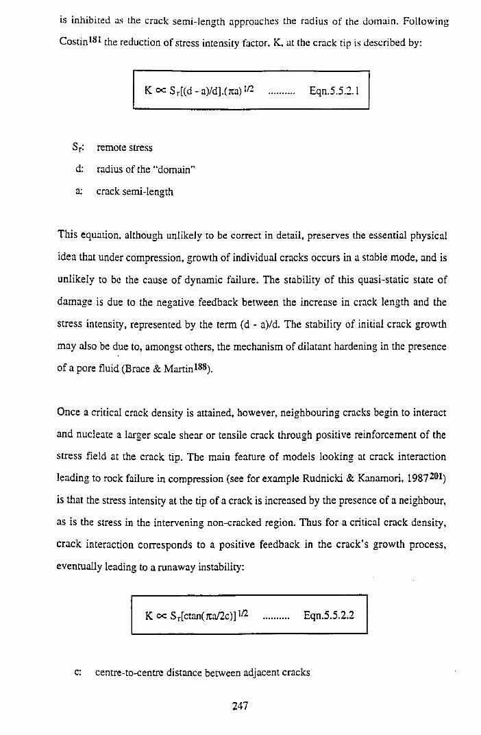
is inhibited as the crack semi-length approaches the radius of the domain. Following

Costin181 the reduction of stress intensity factor, K, at the crack tip is described by:

K °c S r[(d - a)/d].(7ta)1/2 .......... Eqn.5.5.2.1

Sr: remote stress

d: radius of the “domain”

a: crack semi-length

This equation, although unlikely to be correct in detail, preserves the essential physical

idea that under compression, growth of individual cracks occurs in a stable mode, and is

unlikely to be the cause of dynamic failure. The stability of this quasi-static state of

damage is due to the negative feedback between the increase in crack length and the

stress intensity, represented by the term (d - a)/d. The stability of initial crack growth

may also be due to, amongst others, the mechanism of dilatant hardening in the presence

of a pore fluid (Brace & Martin188).

Once a critical crack density is attained, however, neighbouring cracks begin to interact

and nucleate a larger scale shear or tensile crack through positive reinforcement of the

stress field at the crack tip. The main feature of models looking at crack interaction

leading to rock failure in compression (see for example Rudnicki & Kanamori, 1987 201)

is that the stress intensity at the tip of a crack is increased by the presence of a neighbour,

as is the stress in the intervening non-cracked region. Thus for a critical crack density,

crack interaction corresponds to a positive feedback in the crack’s growth process,

eventually leading to a runaway instability:

K o c S r[ctan(7ta/2c)]1/2 .......... Eqn.5.5.2.2

c: centre-to-centre distance between adjacent cracks

247

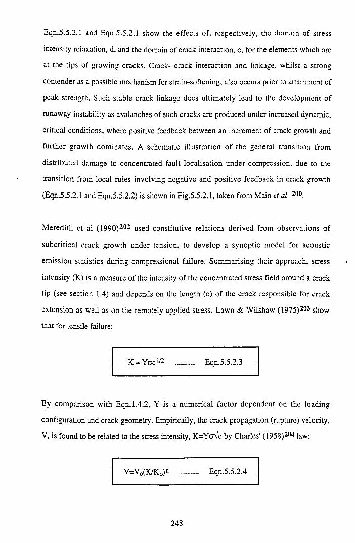
Eqn.5.5.2.1 and Eqn.5.5.2.1 show the effects of, respectively, the domain of stress

intensity relaxation, d, and the domain of crack interaction, c, for the elements which are

at the tips of growing cracks. Crack- crack interaction and linkage, whilst a strong

contender as a possible mechanism for strain-softening, also occurs prior to attainment of

peak strength. Such stable crack linkage does ultimately lead to the development of

runaway instability as avalanches of such cracks are produced under increased dynamic,

critical conditions, where positive feedback between an increment of crack growth and

further growth dominates. A schematic illustration o f the general transition from

distributed damage to concentrated fault localisation under compression, due to the

transition from local rules involving negative and positive feedback in crack growth

(Eqn.5.5.2.1 and Eqn.5.5.2.2) is shown in Fig.5.5.2.1, taken from Main et al 200.

M eredith et al (1990)202 used constitutive relations derived from observations of

subcritical crack growth under tension, to develop a synoptic model for acoustic

emission statistics during compressional failure. Summarising their approach, stress

intensity (K) is a measure of the intensity of the concentrated stress field around a crack

tip (see section 1.4) and depends on the length (c) of the crack responsible for crack

extension as well as on the remotely applied stress. Lawn & Wilshaw (1975)203 show

that for tensile failure:

K = Y ac1/2 .......... Eqn.5.5.2.3

By comparison with Eqn. 1.4.2, Y is a numerical factor dependent on the loading

configuration and crack geometry. Empirically, the crack propagation (rupture) velocity,

V, is found to be related to the stress intensity, K=Y<Wc by Charles’ (1958)204 law:

V=V0(K/K0)n .......... Eqn.5.5.2.4

248

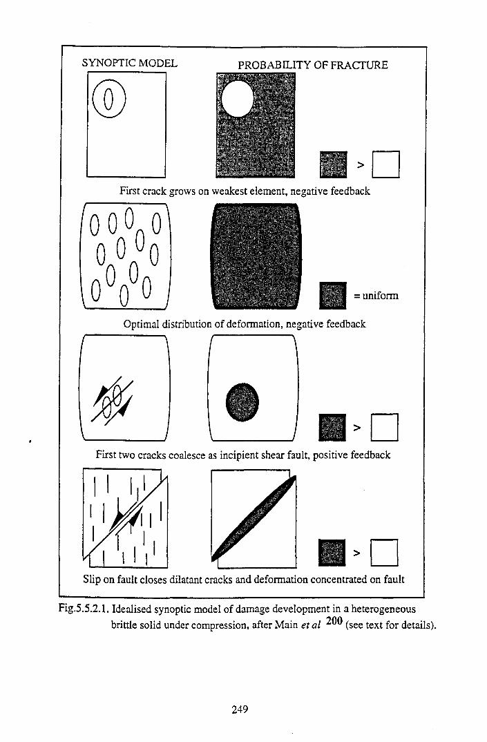
SYNOPTIC MODEL PROBABILITY OF FRACTURE

Optimal distribution of deformation, negative feedback

First two cracks coalesce as incipient shear fault, positive feedback

Slip on fault closes dilatant cracks and deformation concentrated on fault

Fig.5.5.2.1. Idealised synoptic model of damage development in a heterogeneousbrittle solid under compression, after Main et al 200 (see text for details).

249

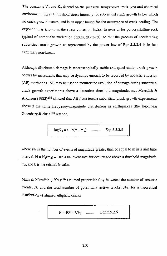
The constants V0 and K« depend on the pressure, temperature, rock type and chemical

environment. K0 is a threshold stress intensity for subcritical crack growth below which

no crack growth occurs, and is an upper bound for the occurrence of crack healing. The

exponent n is known as the stress corrosion index. In general for polycrystalline rock

typical of earhquake nucleation depths, 20<n<60, so that the process of accelerating

subcritical crack growth as represented by the power law of Eqn.5.5.2.4 is in fact

extremely non-linear.

Although distributed damage is macroscopically stable and quasi-static, crack growth

occurs by increments that may be dynamic enough to be recorded by acoustic emission

(AE) monitoring. AE may be used to monitor the evolution of damage during subcritical

crack growth experiments above a detection threshold magnitude, mc. Meredith &

Atkinson (1983)205 showed that AE from tensile subcritical crack growth experiments

showed the same frequency-magnitude distribution as earthquakes (the log-linear

Gutenberg-Richter198 relation):

logNc = a - b(m - m c) .......... Eqn.5.5.2.5

where Nc is the number of events of magnitude greater than or equal to m in a unit time

interval, N = Nc(mc) = 10a is the event rate for occurrence above a threshold magnitude

me, and b is the seismic b-value.

Main & Meredith (1991)206 assumed proportionality between: the number of acoustic

events, N, and the total number of potentially active cracks, N t , for a theoretical

distribution of aligned, elliptical cracks

N = 10a = XNj .......... Eqn.5.5.2.6

250

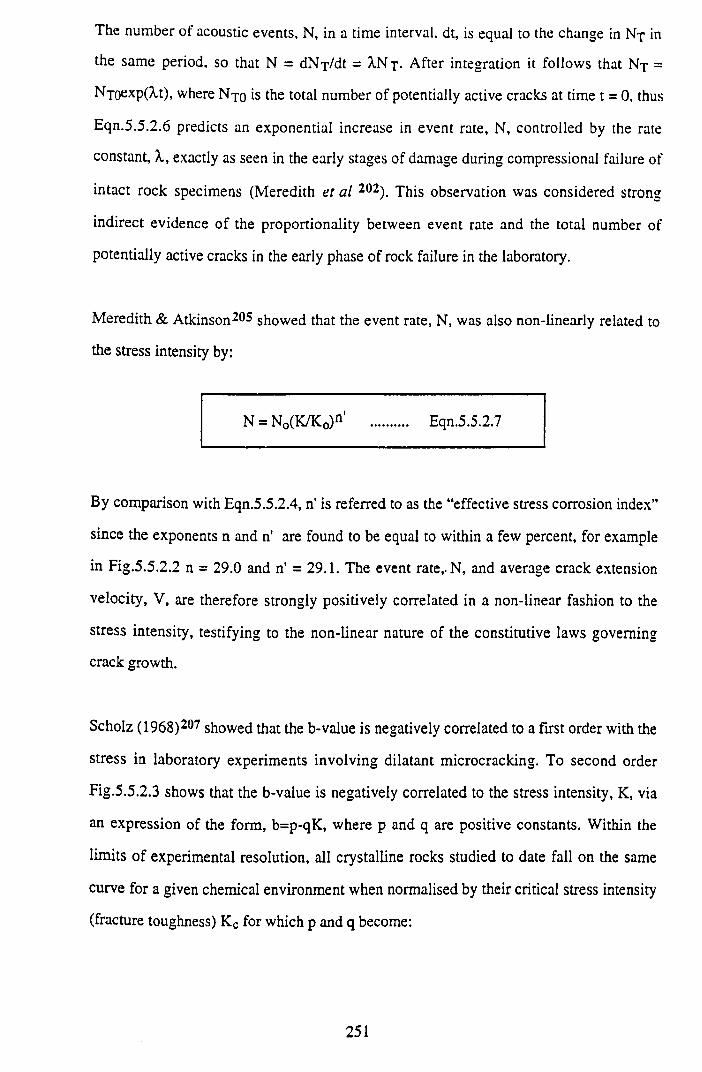
The number of acoustic events, N, in a time interval, dt, is equal to the change in N j in

the same period, so that N = dN j/d t = X.Nt - After integration it follows that N j =

Njoexp(A,t), where N 70 is the total number of potentially active cracks at time t = 0, thus

Eqn.5.5.2.6 predicts an exponential increase in event rate, N, controlled by the rate

constant, X, exactly as seen in the early stages of damage during compressional failure of

intact rock specimens (Meredith et al 202). This observation was considered strong

indirect evidence of the proportionality between event rate and the total number of

potentially active cracks in the early phase of rock failure in the laboratory.

Meredith & Atkinson205 showed that the event rate, N, was also non-linearly related to

the stress intensity by:

N = N0(K/K0)n' .......... Eqn.5.5.2.7

By comparison with Eqn.5.5.2.4, n’ is referred to as the “effective stress corrosion index”

since the exponents n and n' are found to be equal to within a few percent, for example

in Fig.5.5.2.2 n = 29.0 and n' = 29.1. The event rate,. N, and average crack extension

velocity, V, are therefore strongly positively correlated in a non-linear fashion to the

stress intensity, testifying to the non-linear nature of the constitutive laws governing

crack growth.

Scholz (1968)207 showed that the b-value is negatively correlated to a first order with the

stress in laboratory experiments involving dilatant microcracking. To second order

Fig.5.5.2.3 shows that the b-value is negatively correlated to the stress intensity, K, via

an expression of the form, b=p-qK, where p and q are positive constants. Within the

limits of experimental resolution, all crystalline rocks studied to date fall on the same

curve for a given chemical environment when normalised by their critical stress intensity

(fracture toughness) Kc for which p and q become:

251

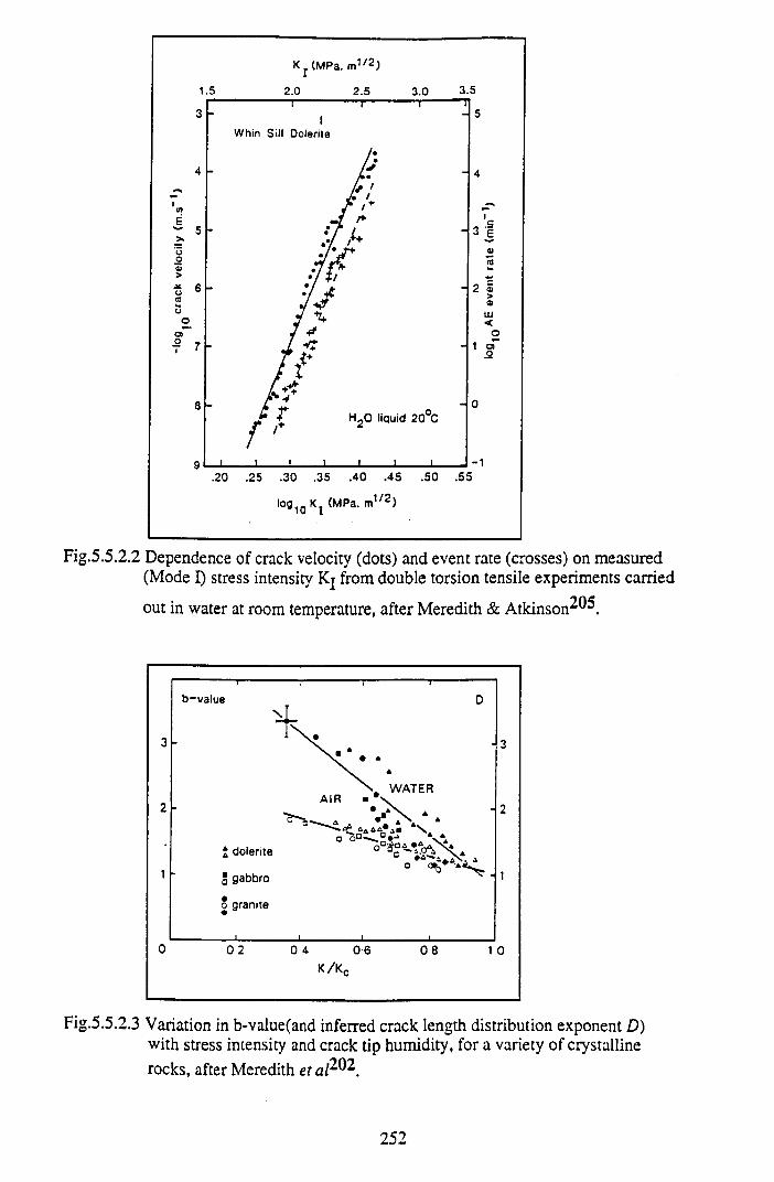
K j (MPa. m1/2)

1.5 2 .0 2 .5 3 .0 3 .5

Fig.5.5.2.2 Dependence of crack velocity (dots) and event rate (crosses) on measured (Mode I) stress intensity Kj from double torsion tensile experiments carried

out in water at room temperature, after Meredith & A tk in s o n ^ .

K/Kc

Fig.5.5.2.3 Variation in b-value(and inferred crack length distribution exponent D) with stress intensity and crack tip humidity, for a variety of crystallinerocks, after Meredith et a l~ ^.

252

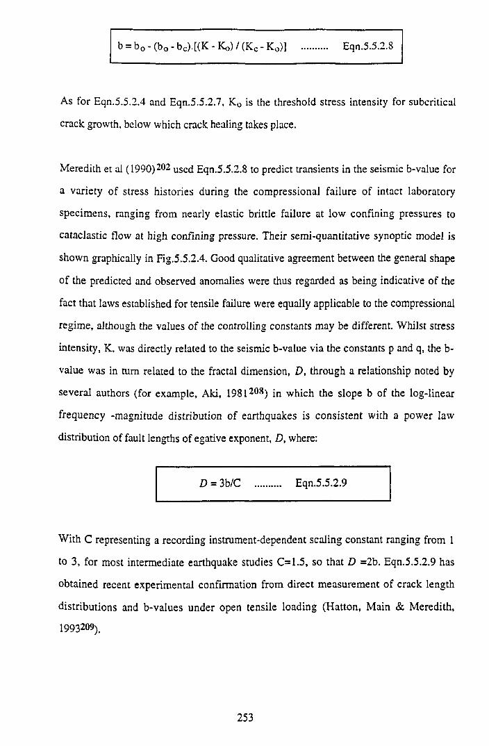
b = bG - (bQ - b c).[(K - Ko) / (Kc - K0)] Eqn.5.5.2.8

As for Eqn.5.5.2.4 and Eqn.5.5.2.7, K0 is the threshold stress intensity for subcritical

crack growth, below which crack healing takes place.

Meredith et al (1990)202 used Eqn.5.5.2.8 to predict transients in the seismic b-value for

a variety of stress histories during the compressional failure of intact laboratory

specimens, ranging from nearly elastic brittle failure at low confining pressures to

cataclastic flow at high confining pressure. Their semi-quantitative synoptic model is

shown graphically in Fig.5.5.2.4. Good qualitative agreement between the general shape

of the predicted and observed anomalies were thus regarded as being indicative of the

fact that laws established for tensile failure were equally applicable to the compressional

regime, although the values of the controlling constants may be different. Whilst stress

intensity, K, was directly related to the seismic b-value via the constants p and q, the b-

value was in turn related to the fractal dimension, D, through a relationship noted by

several authors (for example, Aki, 1981208) jn which the slope b of the log-linear

frequency -magnitude distribution of earthquakes is consistent with a power law

distribution of fault lengths of egative exponent, D, where:

D = 3b/C .......... Eqn.5.5.2.9

With C representing a recording instrument-dependent scaling constant ranging from 1

to 3, for most intermediate earthquake studies C=1.5, so that D =2b. Eqn.5.5.2.9 has

obtained recent experimental confirmation from direct measurement of crack length

distributions and b-values under open tensile loading (Hatton, Main & Meredith,

1993209).

253

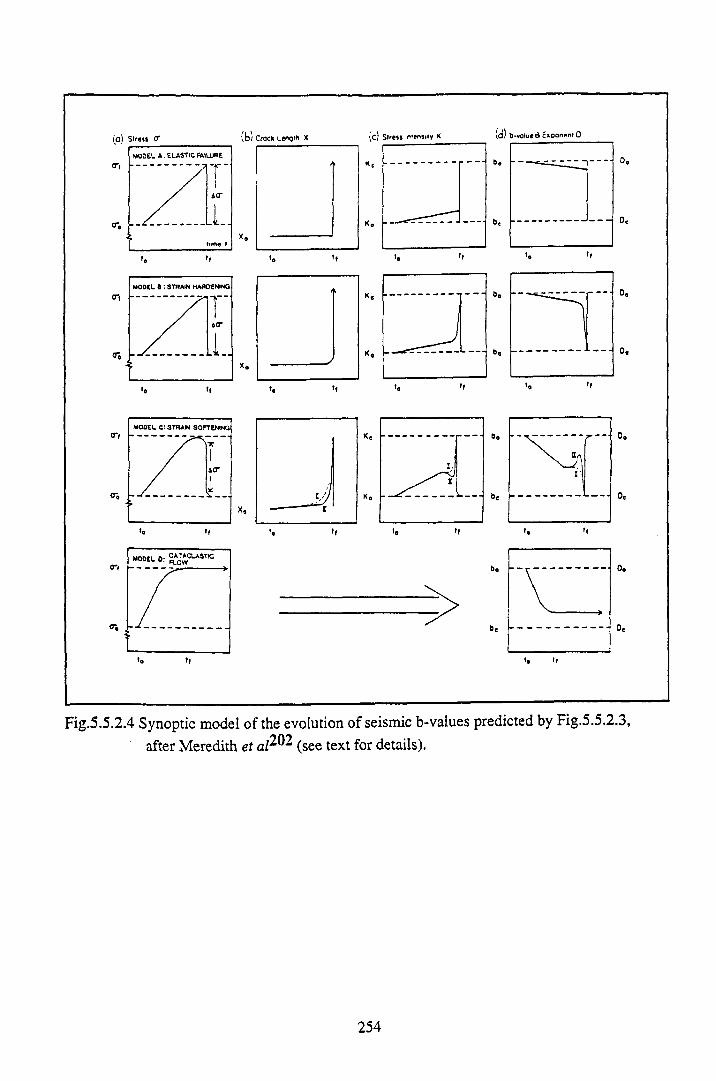
tC! Str«$t O' (b) Croc» Length X (c) Siren intensity K Id) b-voluetJ c»oonent 0

Oc

0.

Oe

Fig.5.5.2.4 Synoptic model of the evolution of seismic b-values predicted by Fig.5.5.2.3, after Meredith et (see text for details).

254

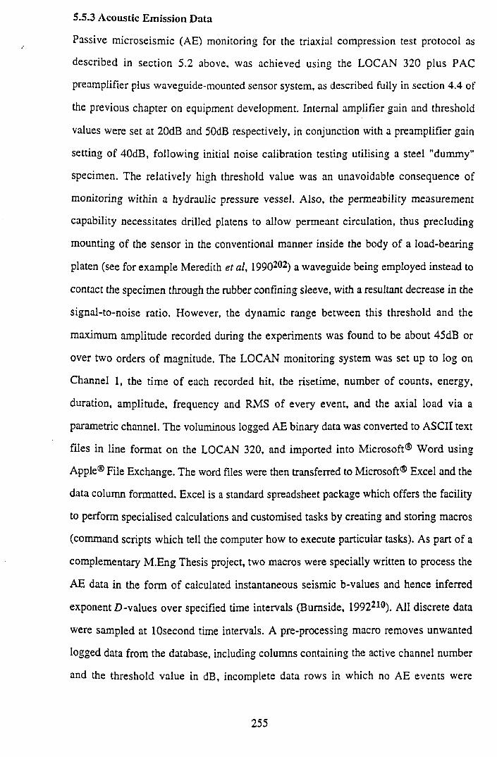
5.5.3 Acoustic Emission Data

Passive microseismic (AE) monitoring for the triaxial compression test protocol as

described in section 5.2 above, was achieved using the LOCAN 320 plus PAC

preamplifier plus waveguide-mounted sensor system, as described fully in section 4.4 of

the previous chapter on equipment development. Internal amplifier gain and threshold

values were set at 20dB and 50dB respectively, in conjunction with a preamplifier gain

setting of 40dB, following initial noise calibration testing utilising a steel "dummy"

specimen. The relatively high threshold value was an unavoidable consequence of

monitoring within a hydraulic pressure vessel. Also, the permeability measurement

capability necessitates drilled platens to allow permeant circulation, thus precluding

mounting of the sensor in the conventional manner inside the body of a load-bearing

platen (see for example Meredith et al, 1990202) a waveguide being employed instead to

contact the specimen through the rubber confining sleeve, with a resultant decrease in the

signal-to-noise ratio. However, the dynamic range between this threshold and the

maximum amplitude recorded during the experiments was found to be about 45dB or

over two orders o f magnitude. The LOCAN monitoring system was set up to log on

Channel 1, the time of each recorded hit, the risetime, number of counts, energy,

duration, amplitude, frequency and RMS of every event, and the axial load via a

parametric channel. The voluminous logged AE binary data was converted to ASCII text

files in line format on the LOCAN 320, and imported into Microsoft® W ord using

Apple® File Exchange. The word files were then transferred to Microsoft® Excel and the

data column formatted. Excel is a standard spreadsheet package which offers the facility

to perform specialised calculations and customised tasks by creating and storing macros

(command scripts which tell the computer how to execute particular tasks). As part of a

complementary M.Eng Thesis project, two macros were specially written to process the

AE data in the form of calculated instantaneous seismic b-values and hence inferred

exponent D -values over specified time intervals (Burnside, 1992210). All discrete data

were sampled at lOsecond time intervals. A pre-processing macro removes unwanted

logged data from the database, including columns containing the active channel number

and the threshold value in dB, incomplete data rows in which no AE events were

255

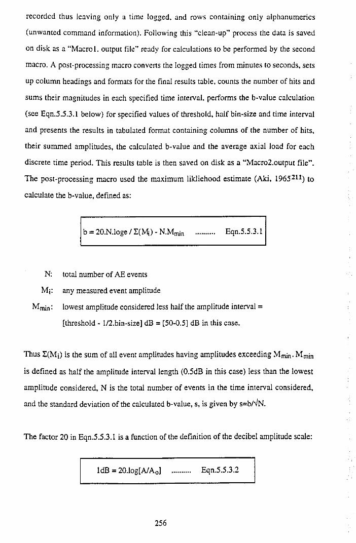
recorded thus leaving only a time logged, and rows containing only alphanumerics

(unwanted command information). Following this “clean-up" process the data is saved

on disk as a “Macro 1. output file” ready for calculations to be performed by the second

macro. A post-processing macro converts the logged times from minutes to seconds, sets

up column headings and formats for the final results table, counts the number of hits and

sums their magnitudes in each specified time interval, performs the b-value calculation

(see Eqn.5.5.3.1 below) for specified values of threshold, half bin-size and time interval

and presents the results in tabulated format containing columns of the number of hits,

their summed amplitudes, the calculated b-value and the average axial load for each

discrete time period. This results table is then saved on disk as a “Macro2.output file” .

The post-processing macro used the maximum likliehood estimate (Aki, 1965211) to

calculate the b-value, defined as:

b = 20.N.loge / 1 (H ) - N.Mmin .......... Eqn.5.5.3.1

N: total number of AE events

Mi: any measured event amplitude

Mmin: lowest amplitude considered less half the amplitude interval =

[threshold - 1/2.bin-size] dB = [50-0.5] dB in this case.

Thus I(M j) is the sum of all event amplitudes having amplitudes exceeding Mmin-

is defined as half the amplitude interval length (0.5dB in this case) less than the lowest

amplitude considered, N is the total number of events in the time interval considered,

and the standard deviation of the calculated b-value, s, is given by s=b/VN.

The factor 20 in Eqn.5.5.3.1 is a function of the definition of the decibel amplitude scale:

ldB = 20.1og[A/Ao] .......... Eqn.5.5.3.2

256

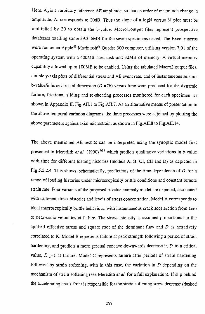
Here, Ac is an arbitrary reference AE amplitude, so that an order of magnitude change in

amplitude. A, corresponds to 20dB. Thus the slope of a logN versus M plot must be

multiplied by 20 to obtain the b-value. Macro 1.output files represent prospective

databases totalling some 39.346MB for the seven specimens tested. The Excel macros

were run on an Apple® Macintosh® Quadra 900 computer, utilising version 7.01 of the

operating system with a 400MB hard disk and 32MB of memory. A virtual memory

capability allowed up to 100MB to be enabled. Using the tabulated Macro2.output files,

double y-axis plots of differential stress and AE event rate, and of instantaneous seismic

b-value/inferred fractal dimension (D =2b) versus time were produced for the dynamic

failure, frictional sliding and re-shearing processes monitored for each specimen, as

shown in Appendix II, Fig. All. 1 to Fig.AH.7. As an alternative means of presentation to

the above temporal variation diagrams, the three processes were adjoined by plotting the

above parameters against axial microstrain, as shown in Fig.AII.8 to Fig.AII.14.

The above mentioned AE results can be interpreted using the synoptic model first

presented in Meredith et al (1990)202 which predicts qualitative variations in b-value

with time for different loading histories (models A, B, Cl, CII and D) as depicted in

Fig.5.5.2.4. This shows, schematically, predictions of the time dependence of D for a

range of loading histories under microscopically brittle conditions and constant remote

strain rate. Four variants of the proposed b-value anomaly model are depicted, associated

with different stress histories and levels of stress concentration. Model A corresponds to

ideal macroscopically brittle behaviour, with instantaneous crack acceleration from zero

to near-sonic velocities at failure. The stress intensity is assumed proportional to the

applied effective stress and square root of the dominant flaw and D is negatively

correlated to K. Model B represents failure at peak strength following a period of strain

hardening, and predicts a more gradual concave-downwards decrease in D to a critical

value, D C=1 at failure. Model C represents failure after periods of strain hardening

followed by strain softening, with in this case, the variation in D depending on the

mechanism of strain softening (see Meredith et al for a full explanation). If slip behind

the accelerating crack front is responsible for the strain softening stress decrease (dashed

257

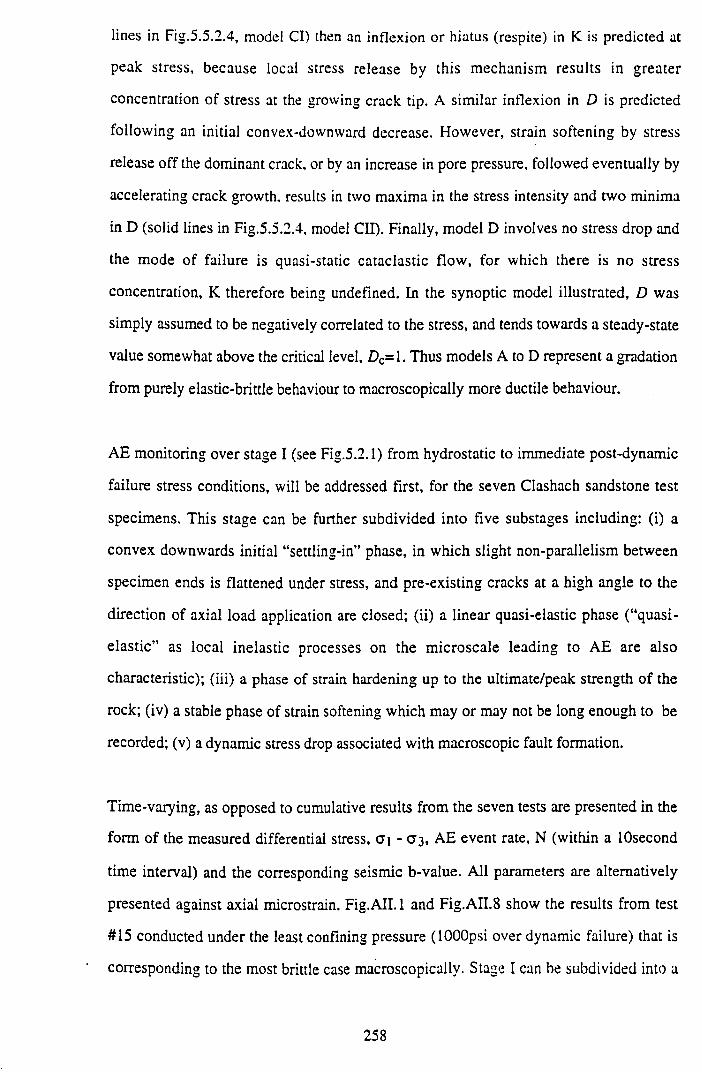
lines in Fig.5.5.2.4, model Cl) then an inflexion or hiatus (respite) in K is predicted at

peak stress, because local stress release by this mechanism results in greater

concentration of stress at the growing crack tip. A similar inflexion in D is predicted

following an initial convex-downward decrease. However, strain softening by stress

release off the dominant crack, or by an increase in pore pressure, followed eventually by

accelerating crack growth, results in two maxima in the stress intensity and two minima

in D (solid lines in Fig.5.5.2.4, model CII). Finally, model D involves no stress drop and

the mode of failure is quasi-static cataclastic flow, for which there is no stress

concentration, K therefore being undefined. In the synoptic model illustrated, D was

simply assumed to be negatively correlated to the stress, and tends towards a steady-state

value somewhat above the critical level, Dc= l. Thus models A to D represent a gradation

from purely elastic-brittle behaviour to macroscopically more ductile behaviour.

AE monitoring over stage I (see Fig.5.2.1) from hydrostatic to immediate post-dynamic

failure stress conditions, will be addressed first, for the seven Clashach sandstone test

specimens. This stage can be further subdivided into five substages including: (i) a

convex downwards initial “settling-in” phase, in which slight non-parallelism between

specimen ends is flattened under stress, and pre-existing cracks at a high angle to the

direction of axial load application are closed; (ii) a linear quasi-elastic phase (“quasi-

elastic” as local inelastic processes on the microscale leading to AE are also

characteristic); (iii) a phase of strain hardening up to the ultimate/peak strength of the

rock; (iv) a stable phase of strain softening which may or may not be long enough to be

recorded; (v) a dynamic stress drop associated with macroscopic fault formation.

Time-varying, as opposed to cumulative results from the seven tests are presented in the

form of the measured differential stress, Ci - C 3, AE event rate, N (within a lOsecond

time interval) and the corresponding seismic b-value. All parameters are alternatively

presented against axial microstrain. Fig.AIL 1 and Fig.AII.8 show the results from test

#15 conducted under the least confining pressure (lOOOpsi over dynamic failure) that is

corresponding to the most brittle case macroscopically. Stage I can be subdivided into a

258

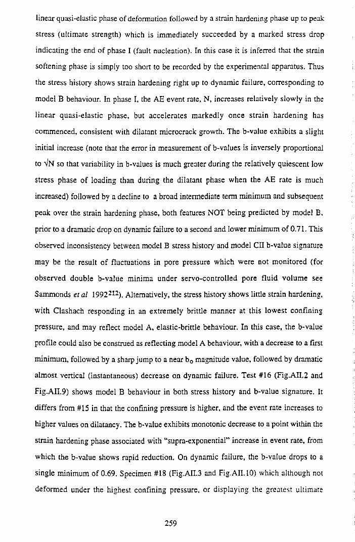
linear quasi-elastic phase of deformation followed by a strain hardening phase up to peak

stress (ultimate strength) which is immediately succeeded by a marked stress drop

indicating the end of phase I (fault nucleation). In this case it is inferred that the strain

softening phase is simply too short to be recorded by the experimental apparatus. Thus

the stress history shows strain hardening right up to dynamic failure, corresponding to

model B behaviour. In phase I, the AE event rate, N, increases relatively slowly in the

linear quasi-elastic phase, but accelerates markedly once strain hardening has

commenced, consistent with dilatant microcrack growth. The b-value exhibits a slight

initial increase (note that the error in measurement of b-values is inversely proportional

to Vn so that variability in b-values is much greater during the relatively quiescent low

stress phase of loading than during the dilatant phase when the AE rate is much

increased) followed by a decline to a broad intermediate term minimum and subsequent

peak over the strain hardening phase, both features NOT being predicted by model B,

prior to a dramatic drop on dynamic failure to a second and lower minimum of 0.71. This

observed inconsistency between model B stress history and model CII b-value signature

may be the result of fluctuations in pore pressure which were not monitored (for

observed double b-value minima under servo-controlled pore fluid volume see

Sammonds etal 1992212). Alternatively, the stress history shows little strain hardening,

with Clashach responding in an extremely brittle manner at this lowest confining

pressure, and may reflect model A, elastic-brittle behaviour. In this case, the b-value

profile could also be construed as reflecting model A behaviour, with a decrease to a first

minimum, followed by a sharp jump to a near bQ magnitude value, followed by dramatic

almost vertical (instantaneous) decrease on dynamic failure. Test #16 (Fig.AII.2 and

Fig.AII.9) shows model B behaviour in both stress history and b-value signature. It

differs from #15 in that the confining pressure is higher, and the event rate increases to

higher values on dilatancy. The b-value exhibits monotonic decrease to a point within the

strain hardening phase associated with “supra-exponential” increase in event rate, from

which the b-value shows rapid reduction. On dynamic failure, the b-value drops to a

single minimum of 0.69. Specimen #18 (Fig.AII.3 and Fig.AIL 10) which although not

deformed under the highest confining pressure, or displaying the greatest ultimate

259

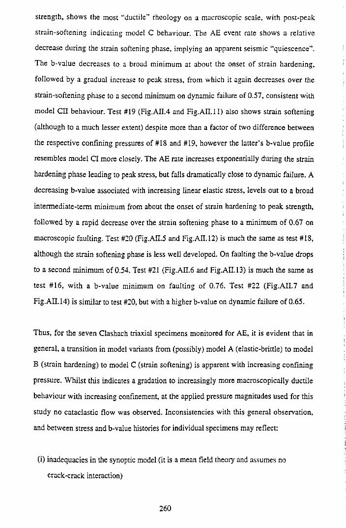
strength, shows the most “ductile” rheology on a macroscopic scale, with post-peak

strain-softening indicating model C behaviour. The AE event rate shows a relative

decrease during the strain softening phase, implying an apparent seismic “quiescence”.

The b-value decreases to a broad minimum at about the onset of strain hardening,

followed by a gradual increase to peak stress, from which it again decreases over the

strain-softening phase to a second minimum on dynamic failure of 0.57, consistent with

model CII behaviour. Test #19 (Fig.AII.4 and F ig .A II.il) also shows strain softening

(although to a much lesser extent) despite more than a factor of two difference between

the respective confining pressures of #18 and #19, however the latter’s b-value profile

resembles model Cl more closely. The AE rate increases exponentially during the strain

hardening phase leading to peak stress, but falls dramatically close to dynamic failure. A

decreasing b-value associated with increasing linear elastic stress, levels out to a broad

intermediate-term minimum from about the onset of strain hardening to peak strength,

followed by a rapid decrease over the strain softening phase to a minimum of 0.67 on

macroscopic faulting. Test #20 (Fig.AII.5 and Fig.AII.12) is much the same as test #18,

although the strain softening phase is less well developed. On faulting the b-value drops

to a second minimum of 0.54. Test #21 (Fig.AII.6 and Fig.AH 13) is much the same as

test #16, with a b-value minimum on faulting of 0.76. Test #22 (Fig.AII.7 and

Fig.AD. 14) is similar to test #20, but with a higher b-value on dynamic failure of 0.65.

Thus, for the seven Clashach triaxial specimens monitored for AE, it is evident that in

general, a transition in model variants from (possibly) model A (elastic-brittle) to model

B (strain hardening) to model C (strain softening) is apparent with increasing confining

pressure. Whilst this indicates a gradation to increasingly more macroscopically ductile

behaviour with increasing confinement, at the applied pressure magnitudes used for this

study no cataclastic flow was observed. Inconsistencies with this general observation,

and between stress and b-value histories for individual specimens may reflect:

(i) inadequacies in the synoptic model (it is a mean field theory and assumes no

crack-crack interaction)

260

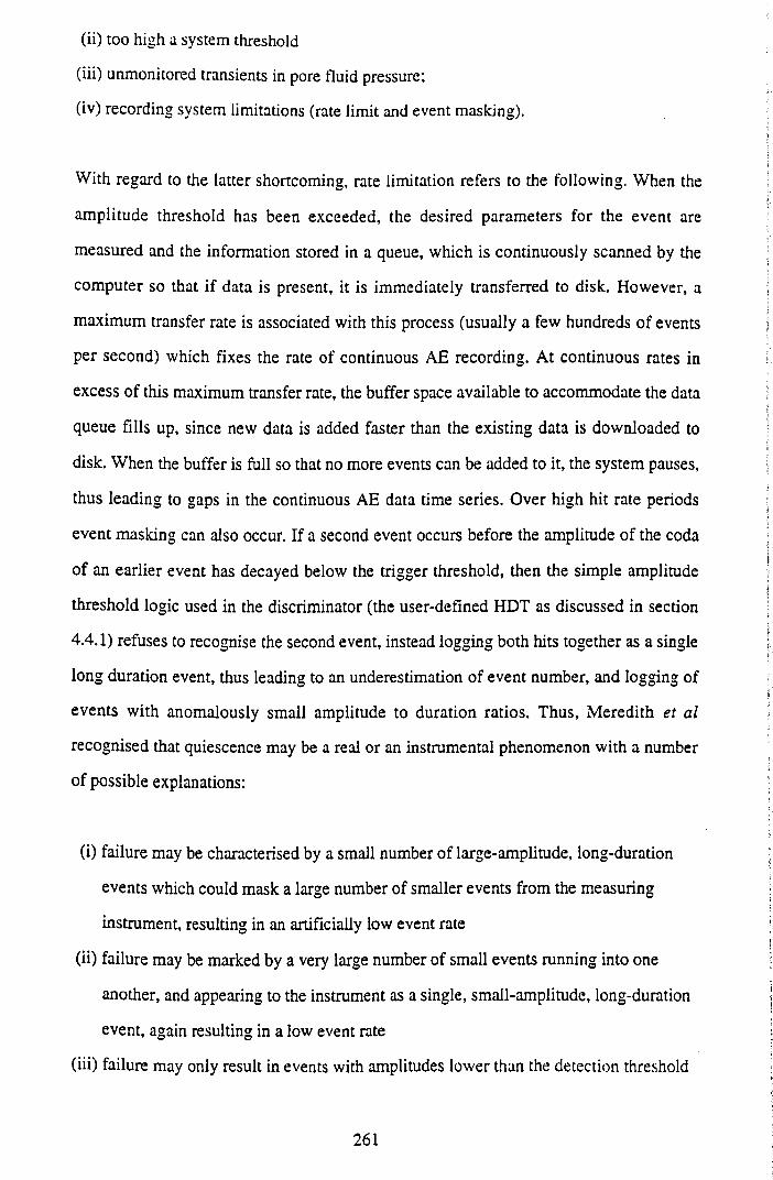
(ii) too high a system threshold

(iii) unmonitored transients in pore fluid pressure;

(iv) recording system limitations (rate limit and event masking).

With regard to the latter shortcoming, rate limitation refers to the following. When the

amplitude threshold has been exceeded, the desired parameters for the event are

measured and the information stored in a queue, which is continuously scanned by the

computer so that if data is present, it is immediately transferred to disk. However, a

maximum transfer rate is associated with this process (usually a few hundreds of events

per second) which fixes the rate of continuous AE recording. At continuous rates in

excess of this maximum transfer rate, the buffer space available to accommodate the data

queue fills up, since new data is added faster than the existing data is downloaded to

disk. When the buffer is full so that no more events can be added to it, the system pauses,

thus leading to gaps in the continuous AE data time series. Over high hit rate periods

event masking can also occur. If a second event occurs before the amplitude of the coda

of an earlier event has decayed below the trigger threshold, then the simple amplitude

threshold logic used in the discriminator (the user-defined HDT as discussed in section

4.4.1) refuses to recognise the second event, instead logging both hits together as a single

long duration event, thus leading to an underestimation of event number, and logging of

events with anomalously small amplitude to duration ratios. Thus, M eredith et al

recognised that quiescence may be a real or an instrumental phenomenon with a number

of possible explanations:

(i) failure may be characterised by a small number of large-amplitude, long-duration

events which could mask a large number of smaller events from the measuring

instrument, resulting in an artificially low event rate

(ii) failure may be marked by a very large number of small events running into one

another, and appearing to the instrument as a single, small-amplitude, long-duration

event, again resulting in a low event rate

(iii) failure may only result in events with amplitudes lower than the detection threshold

261

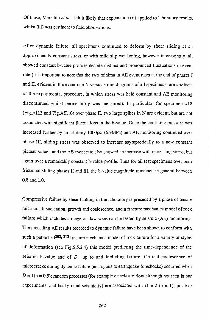
Of these, Meredith et al felt it likely that explanation (ii) applied to laboratory results,

whilst (iii) was pertinent to field observations.

A fter dynamic failure, all specimens continued to deform by shear sliding at an

approximately constant stress, or with mild slip weakening, however interestingly, all

showed constant b-value profiles despite distinct and pronounced fluctuations in event

rate (it is important to note that the two minima in AE event rates at the end of phases I

and II, evident in the event rate N versus strain diagrams of all specimens, are artefacts

o f the experimental procedure, in which stress was held constant and AE monitoring

discontinued whilst permeability was measured). In particular, for specimen #18

(Fig.AII.3 and Fig.AIL 10) over phase II, two large spikes in N are evident, but are not

associated with significant fluctuations in the b-value. Once the confining pressure was

increased further by an arbitrary lOOOpsi (6.9MPa) and AE monitoring continued over

phase III, sliding stress was observed to increase asymptotically to a new constant

plateau value, and the AE event rate also showed an increase with increasing stress, but

again over a remarkably constant b-value profile. Thus for all test specimens over both

frictional sliding phases II and HI, the b-value magnitude remained in general between

0.8 and 1.0.

Compressive failure by shear faulting in the laboratory is preceded by a phase of tensile

microcrack nucleation, growth and coalescence, and a fracture mechanics model of rock

failure which includes a range of flaw sizes can be tested by seismic (AE) monitoring.

The preceding AE results recorded to dynamic failure have been shown to conform with

such a published202*213 fracture mechanics model of rock failure for a variety of styles

o f deformation (see Fig.5.5.2.4) this model predicting the time-dependence of the

seismic b-value and of D up to and including failure. Critical coalescence of

microcracks during dynamic failure (analogous to earthquake foreshocks) occurred when

D - l(b = 0.5); random processes (for example cataclastic flow although not seen in our

experiments, and background seismicity) are associated with D = 2 (b = 1;; positive

262

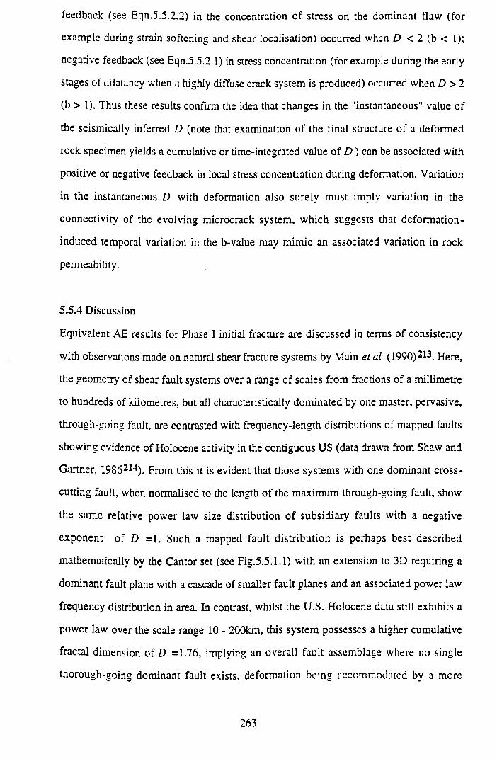
feedback (see Eqn.5.5.2.2) in the concentration of stress on the dominant flaw (for

example during strain softening and shear localisation) occurred when D < 2 (b < l);

negative feedback (see Eqn.5.5.2.1) in stress concentration (for example during the early

stages of dilatancy when a highly diffuse crack system is produced) occurred when D >2

(b > 1). Thus these results confirm the idea that changes in the "instantaneous" value of

the seismically inferred D (note that examination of the final structure o f a deformed

rock specimen yields a cumulative or time-integrated value of D ) can be associated with

positive or negative feedback in local stress concentration during deformation. Variation

in the instantaneous D with deformation also surely must imply variation in the

connectivity of the evolving microcrack system, which suggests that deformation -

induced temporal variation in the b-value may mimic an associated variation in rock

permeability.

5.5.4 Discussion

Equivalent AE results for Phase I initial fracture are discussed in terms of consistency

with observations made on natural shear fracture systems by Main etal (1990)213. Here,

the geometry of shear fault systems over a range of scales from fractions of a millimetre

to hundreds of kilometres, but all characteristically dominated by one master, pervasive,

through-going fault, are contrasted with frequency-length distributions of mapped faults

showing evidence of Holocene activity in the contiguous US (data drawn from Shaw and

Gartner, 1986214). From this it is evident that those systems with one dominant cross­

cutting fault, when normalised to the length of the maximum through-going fault, show

the same relative power law size distribution of subsidiary faults with a negative

exponent of D =1. Such a mapped fault distribution is perhaps best described

mathematically by the Cantor set (see Fig.5.5.1.1) with an extension to 3D requiring a

dominant fault plane with a cascade of smaller fault planes and an associated power law

frequency distribution in area. In contrast, whilst the U.S. Holocene data still exhibits a

power law over the scale range 10 - 200km, this system possesses a higher cumulative

fractal dimension of D =1.76, implying an overall fault assemblage where no single

thorough-going dominant fault exists, deformation being accommodated by a more

263

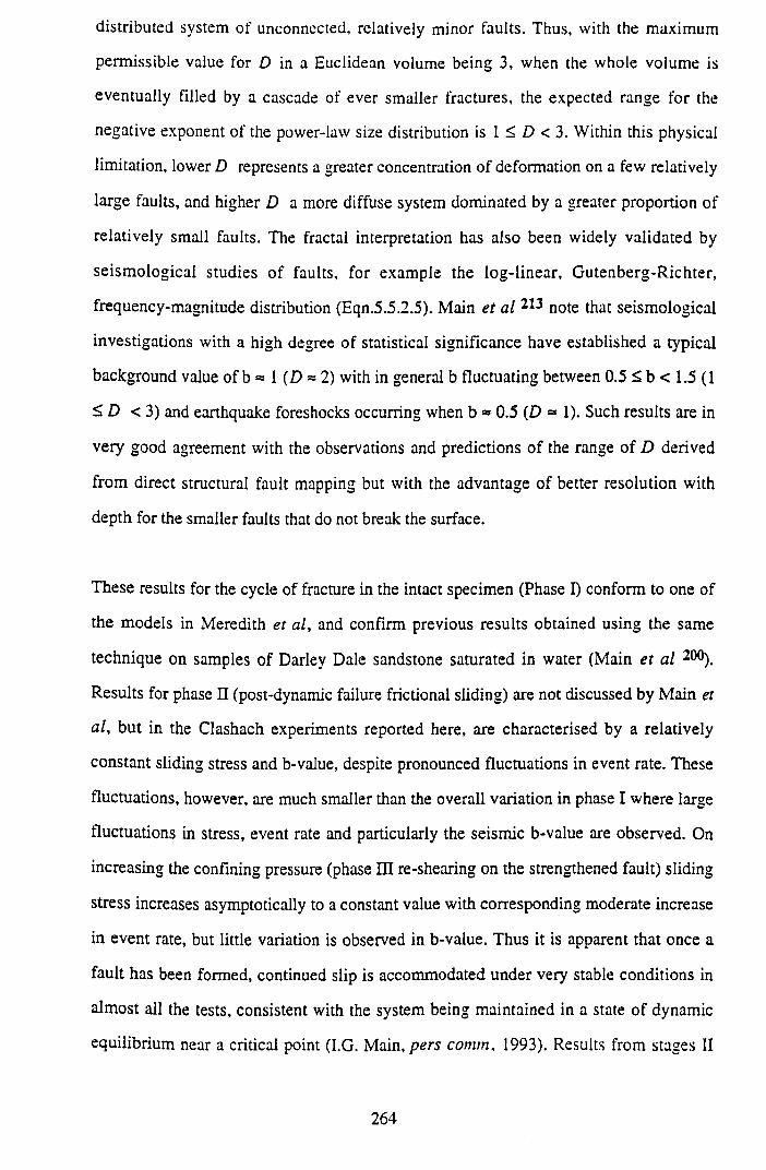
distributed system of unconnected, relatively minor faults. Thus, with the maximum

permissible value for D in a Euclidean volume being 3, when the whole volume is

eventually filled by a cascade of ever smaller fractures, the expected range for the

negative exponent of the power-law size distribution is 1 < D < 3. Within this physical

limitation, lower D represents a greater concentration of deformation on a few relatively

large faults, and higher D a more diffuse system dominated by a greater proportion of

relatively small faults. The fractal interpretation has also been widely validated by

seism ological studies o f faults, for example the log-linear, Gutenberg-Richter,

frequency-magnitude distribution (Eqn.5.5.2.5). Main et al 213 note that seismological

investigations with a high degree of statistical significance have established a typical

background value of b = 1 (D ~ 2) with in general b fluctuating between 0.5 < b < 1.5 (1

^ D < 3) and earthquake foreshocks occurring when b * 0.5 (D « 1). Such results are in

very good agreement with the observations and predictions of the range of D derived

from direct structural fault mapping but with the advantage of better resolution with

depth for the smaller faults that do not break the surface.

These results for the cycle of fracture in the intact specimen (Phase I) conform to one of

the models in Meredith et al, and confirm previous results obtained using the same

technique on samples of Darley Dale sandstone saturated in water (Main et al 20°).

Results for phase II (post-dynamic failure frictional sliding) are not discussed by Main et

al, but in the Clashach experiments reported here, are characterised by a relatively

constant sliding stress and b-value, despite pronounced fluctuations in event rate. These

fluctuations, however, are much smaller than the overall variation in phase I where large

fluctuations in stress, event rate and particularly the seismic b-value are observed. On

increasing the confining pressure (phase III re-shearing on the strengthened fault) sliding

stress increases asymptotically to a constant value with corresponding moderate increase

in event rate, but little variation is observed in b-value. Thus it is apparent that once a

fault has been formed, continued slip is accommodated under very stable conditions in

almost all the tests, consistent with the system being maintained in a state of dynamic

equilibrium near a critical point (I.G. Main, pers comm, 1993). Results from stages II

264

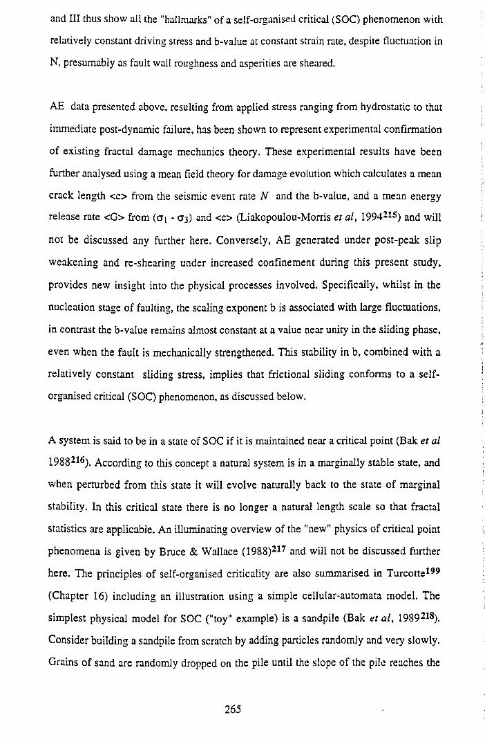
and III thus show all the "hallmarks" of a self-organised critical (SOC) phenomenon with

relatively constant driving stress and b-value at constant strain rate, despite fluctuation in

N, presumably as fault wall roughness and asperities are sheared.

AE data presented above, resulting from applied stress ranging from hydrostatic to that

immediate post-dynamic failure, has been shown to represent experimental confirmation

of existing fractal damage mechanics theory. These experimental results have been

further analysed using a mean field theory for damage evolution which calculates a mean

crack length <c> from the seismic event rate N and the b-value, and a mean energy

release rate <G> from (<7 i - <73) and < 0 (Liakopoulou-Morris et al, 1994215) and will

not be discussed any further here. Conversely, AE generated under post-peak slip

weakening and re-shearing under increased confinement during this present study,

provides new insight into the physical processes involved. Specifically, whilst in the

nucleation stage of faulting, the scaling exponent b is associated with large fluctuations,

in contrast the b-value remains almost constant at a value near unity in the sliding phase,

even when the fault is mechanically strengthened. This stability in b, combined with a

relatively constant sliding stress, implies that frictional sliding conforms to a self-

organised critical (SOC) phenomenon, as discussed below.

A system is said to be in a state of SOC if it is maintained near a critical point (Bak et al

198821<>). According to this concept a natural system is in a marginally stable state, and

when perturbed from this state it will evolve naturally back to the state of marginal

stability. In this critical state there is no longer a natural length scale so that fractal

statistics are applicable. An illuminating overview of the "new" physics of critical point

phenomena is given by Bruce & Wallace (1988)217 and will not be discussed further

here. The principles of self-organised criticality are also summarised in Turcotte199

(Chapter 16) including an illustration using a simple cellular-automata model. The

simplest physical model for SOC ("toy" example) is a sandpile (Bak et al, 1989218).

Consider building a sandpile from scratch by adding particles randomly and very slowly.

Grains of sand are randomly dropped on the pile until the slope of the pile reaches the

265

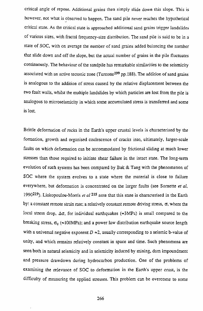
critical angle of repose. Additional grains then simply slide down this slope. This is

however, not what is observed to happen. The sand pile never reaches the hypothetical

critical state. As the critical state is approached additional sand grains trigger landslides

of various sizes, with fractal frequency-size distribution. The sand pile is said to be in a

state of SOC, with on average the number of sand grains added balancing the number

that slide down and off the slope, but the actual number of grains in the pile fluctuates

continuously. The behaviour of the sandpile has remarkable similarities to the seismicity

associated with an active tectonic zone (Turcotte199 pp.188). The addition of sand grains

is analogous to the addition of stress caused by the relative displacement between the

two fault walls, whilst the multiple landslides by which particles are lost from the pile is

analogous to microseismicity in which some accumulated stress is transferred and some

is lost.

Brittle deformation of rocks in the Earth's upper crustal levels is characterised by the

formation, growth and organised coalescence of cracks into, ultimately, larger-scale

faults on which deformation can be accommodated by frictional sliding at much lower

stresses than those required to initiate shear failure in the intact state. The long-term

evolution o f such systems has been compared by Bak & Tang with the phenomenon of

SOC where the system evolves to a state where the material is close to failure

everywhere, but deformation is concentrated on the larger faults (see Somette et al,

1990219). Liakopoulou-Morris et a l215 note that this state is characterised in the Earth

by: a constant remote strain rate; a relatively constant remote driving stress, c , where the

local stress drop, Ac, for individual earthquakes (=3MPa) is small compared to the

breaking stress, c c (»lOOMPa); and a power law distribution earthquake source length

with a universal negative exponent D ~2, usually corresponding to a seismic b-value of

unity, and which remains relatively constant in space and time. Such phenomena are

seen both in natural seismicity and in seismicity induced by mining, dam impoundment

and pressure drawdown during hydrocarbon production. One of the problems of

examining the relevance of SOC to deformation in the Earth's upper crust, is the

difficulty of measuring the applied stresses. This problem can be overcome to some

266

extent in the laboratory where experimental conditions can be controlled, but where, for

example, it is impossible with current technology to achieve strain rates as low as those

applicable in the Earth (even for cases of induced seismicity where there is often a time

delay of months or years to the onset of earthquakes). From the experiments reported

here, in contrast to stage I, the results from stages II and III do show evidence of

universal SOC, with relatively constant b and a at constant strain rate, even though N

may fluctuate as a particular asperity on the fresh fault surface is sheared off. This is

fully consistent with recent treatment of faulting as a self-organised process which

maintains the system in a universal critical state, implying a degree of order in the

formation of fault gouge and continued shearing. Whilst it might be expected for the b-

value to evolve with time as surfaces become worn and asperity shearing is replaced by

frictional wear of debris as a slip mechanism, this was not observed for the Clashach test

programme (admittedly involving only minor slip displacements) implying that

roughening processes such as grain-plucking or "brecciation" are also taking place to

balance the comminution of gouge which would tend to help smooth the contact

surfaces. This has obvious implications for the long-term permeability of fault zones, and

further, it is tentatively suggested that AE statistics may provide a suitable basis on

which to build a micromechanical theory of rock friction.

267

6. A R TIFIC IA L FAULT GOUGE GENERATED UNDER D IR EC T SHEAR

AND TRIAXIAL COM PRESSION CONDITIONS: RESULTS

6.1 IN TRO D U C TIO N

In general, there is not much difference between the fracture mechanics analysis of shear

and tensile cracks (see section 1.4) however one major point of disparity is that, unlike

tensile cracks, shear crack faces are not stress-free even if the surfaces have been well-slid.

Following dynamic shear rupture, gross shear load does not drop to zero, but falls to a

value commensurate with the residual frictional resistance of the plane of sliding.

Importantly, this frictional work acts as an additional energy sink, reducing the amount of

energy available to drive the crack tip. Energy dissipation associated with that part of the

total energy budget expended in frictional traction behind the rupture front, occurs mainly

by thermomechanical processes involving heat generation and grain comminution. The

creation of new surface area in the form of frictional wear debris (fault gouge) is thus

fundamental to fault mechanics, and can also readily be envisaged as a process with first

order control on shear fracture fluid flow potential.

Artificial (experimentally created from laboratory testing) fault gouge samples generated by

the direct shear and triaxial compression test programmes described in Chapters 3 and 5

respectively, are quantified in this Chapter 6, with regard to particle size distributions (see

section 6.2) using both conventional sieving, as well as relatively new laser diffraction

technology to access the sub-micron size range (section 6.3). In section 6.4 the influence of

host lithology on resultant fault gouge distribution is studied, and correlation with frictional

strength, measured in direct shear under constant normal displacement control, explored. In

section 6.5, shear band (induced under triaxial compression) permeabilities are estimated

from pulse decay axial core plug permeability measurements, and correlated with measured

fault gouge distributions, shear band deformation and the applied stress state.

6.2 PARTICLE SIZE DISTRIBUTIONS

Particle size determinations are almost always undertaken in order to obtain information on

the size characteristics of a very large number of panicles, and as the panicles are generally

268

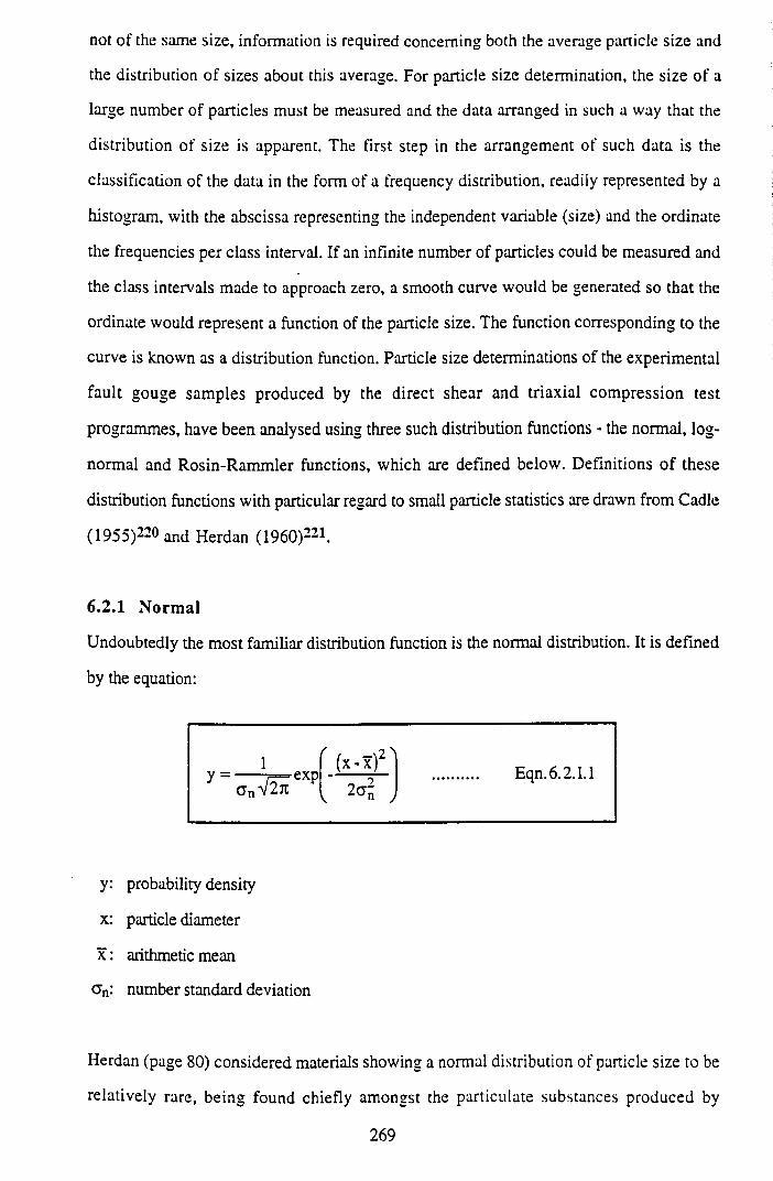
not of the same size, information is required concerning both the average particle size and

the distribution of sizes about this average. For particle size determination, the size of a

large number of particles must be measured and the data arranged in such a way that the

distribution of size is apparent. The first step in the arrangement of such data is the

classification of the data in the form of a frequency distribution, readily represented by a

histogram, with the abscissa representing the independent variable (size) and the ordinate

the frequencies per class interval. If an infinite number of particles could be measured and

the class intervals made to approach zero, a smooth curve would be generated so that the

ordinate would represent a function of the particle size. The function corresponding to the

curve is known as a distribution function. Particle size determinations of the experimental

fault gouge samples produced by the direct shear and triaxial compression test

programmes, have been analysed using three such distribution functions - the normal, log­

normal and Rosin-Rammler functions, which are defined below. Definitions o f these

distribution functions with particular regard to small particle statistics are drawn from Cadle

(1955)220 and Herdan (I960)221.

6.2.1 N orm al

Undoubtedly the most familiar distribution function is the normal distribution. It is defined

by the equation:

y = ■Cn V2 Jt exp ( x - x ) n

jEqn.6.2.1.1

y: probability density

x: particle diameter

x : arithmetic mean

Gn: number standard deviation

Herdan (page 80) considered materials showing a normal distribution of particle size to be

relatively rare, being found chiefly amongst the particulate substances produced by

269

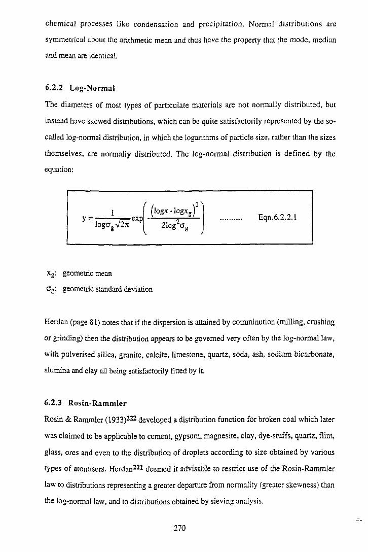
chemical processes like condensation and precipitation. Normal distributions are

symmetrical about the arithmetic mean and thus have the property that the mode, median

and mean are identical.

6.2.2 Log-Norm al

The diameters of most types of particulate materials are not normally distributed, but

instead have skewed distributions, which can be quite satisfactorily represented by the so-

called log-normal distribution, in which the logarithms of particle size, rather than the sizes

themselves, are normally distributed. The log-normal distribution is defined by the

equation:

1 (logx-logxg)2Ean 6 2 2 1

y logagV 2jrCXp 2log2GaK ° J

xg: geometric mean

Gg: geometric standard deviation

Herdan (page 81) notes that if the dispersion is attained by comminution (milling, crushing

or grinding) then the distribution appears to be governed very often by the log-normal law,

with pulverised silica, granite, calcite, limestone, quartz, soda, ash, sodium bicarbonate,

alumina and clay all being satisfactorily fitted by it.

6.2.3 R osin -R am m ler

Rosin & Rammler (1933)222 developed a distribution function for broken coal which later

was claimed to be applicable to cement, gypsum, magnesite, clay, dye-stuffs, quartz, flint,

glass, ores and even to the distribution of droplets according to size obtained by various

types of atomisers. Herdan221 deemed it advisable to restrict use of the Rosin-Rammler

law to distributions representing a greater departure from normality (greater skewness) than

the log-normal law, and to distributions obtained by sieving analysis.

270

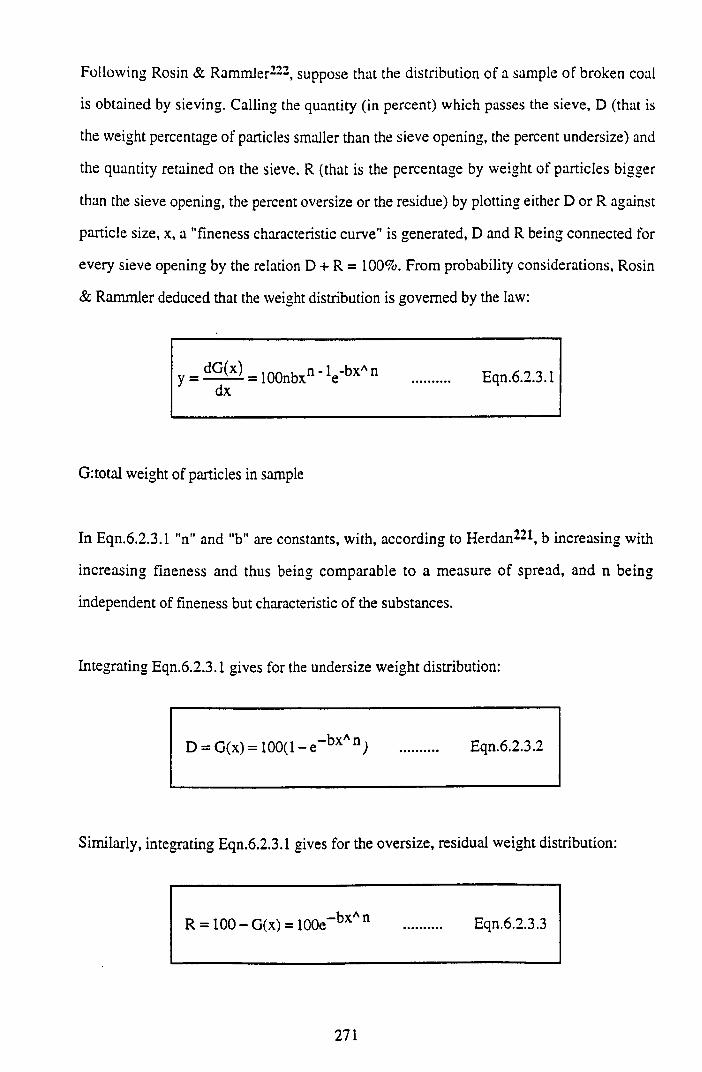
Following Rosin & Rammler222, suppose that the distribution of a sample of broken coal

is obtained by sieving. Calling the quantity (in percent) which passes the sieve, D (that is

the weight percentage of particles smaller than the sieve opening, the percent undersize) and

the quantity retained on the sieve, R (that is the percentage by weight of particles bigger

than the sieve opening, the percent oversize or the residue) by plotting either D or R against

particle size, x, a "fineness characteristic curve" is generated, D and R being connected for

every sieve opening by the relation D + R = 100%. From probability considerations, Rosin

& Rammler deduced that the weight distribution is governed by the law:

y = — — - = 1 OOnbx11 * V bxA n Eqn.6.2.3.1dx

G:total weight of particles in sample

In Eqn.6.2.3.1 "n" and "b" are constants, with, according to Herdan221, b increasing with

increasing fineness and thus being comparable to a measure of spread, and n being

independent of fineness but characteristic of the substances.

Integrating Eqn.6.2.3.1 gives for the undersize weight distribution:

D = G(x) = 100(1- e“ bxA n ) .......... Eqn.6.2.3.2

Similarly, integrating Eqn.6.2.3.1 gives for the oversize, residual weight distribution:

R = 100 - G(x) = 100e_bxA n .......... Eqn.6.2.3.3

271

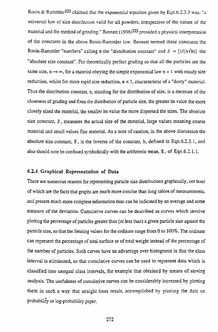
Rosin & Rammler222 claimed that the exponential equation given by Eqn.6.2.3.3 was. "a

universal law of size distribution valid for all powders, irrespective of the nature of the

material and the method of grinding." Bennett (1936)223 provided a physical interpretation

of the constants in the above Rosin-Rammler law. Bennett termed these constants the

Rosin-Rammler "numbers" calling n the "distribution constant" and x = [l/(nVb)] the

"absolute size constant". For theoretically perfect grading so that all the particles are the

same size, n -» °°, for a material obeying the simple exponential law n = 1 with steady size

reduction, whilst for more rapid size reduction, n < 1, characteristic of a "dusty" material.

Thus the distribution constant, n, standing for the distribution of size, is a measure of the

closeness of grading and fixes the distribution of particle size, the greater its value the more

closely sized the material, the smaller its value the more dispersed the sizes. The absolute

size constant, x , measures the actual size of the material, large values meaning coarse

material and small values fine material. As a note of caution, in the above discussion the

absolute size constant, x , is the inverse of the constant, b, defined in Eqn.6.2.3.1, and

also should note be confused symbolically with the arithmetic mean, x , of Eqn.6.2.1.1.

6.2.4 Graphical Representation of Data

There are numerous reasons for representing particle size distributions graphically, not least

of which are the facts that graphs are much more concise than long tables of measurements,

and present much more complete information than can be indicated by an average and some

measure of the deviation. Cumulative curves can be described as curves which involve

plotting the percentage of particles greater than (or less than) a given particle size against the

particle size, so that the limiting values for the ordinate range from 0 to 100%. The ordinate

can represent the percentage of total surface or of total weight instead of the percentage of

the number of particles. Such curves have an advantage over histograms in that the class

interval is eliminated, so that cumulative curves can be used to represent data which is

classified into unequal class intervals, for example that obtained by means o f sieving

analysis. The usefulness of cumulative curves can be considerably increased by plotting

them in such a way that straight lines result, accomplished by plotting the data on

probability or log-probability paper.

272

Suppose that the percentage of the number of particles less than x in diameter, Dn, can be

represented by an equation of the type Dn = fj (x), then a straight line is obtained by

plotting Dn against f; (x). If the diameters of the particles are normally distributed, an

expression in the form of Dn = fj (x) can be obtained by integrating Eqn.6.2.1.1. Whilst

direct integration so as to express Dn as an explicit function of x is not possible, it can be

evaluated from tables of probability integrals. Probability paper represents x on a linear

scale and Dn on a probability scale such that a straight line is obtained when the integrated

form of Eqn.6.2.1.1. is satisfied. Using the terms of the cumulative series (for number

distributions the sums of observations or the percentage frequencies up to specified class

intervals, for weight distributions the weight percent of particles less than or greater than a

given size) percentages are plotted on a probability grid against the corresponding values of

the variable. The cumulative values are plotted not against the class interval centres as are

those of the frequency curve, but against the class interval limits. The straight line of the

graph is some evidence, even though no strict mathematical proof, that the distribution is

governed by the normal law. From such a graph, the mean and standard deviation can be

readily obtained by drawing a horizontal line at the 50% point, the crossing point with the

straight distribution line when projected onto the x-axis giving the arithmetic mean particle

size. Furthermore, projecting the crossing points with the horizontals erected at the

percentage points which correspond to a distance of once the standard deviation on either

side of the mean, that is at either the 84% or the 16% point, approximately, on to the x-

axis, the distance of either of these projections from the mean represents the standard

deviation.

Just as most powders can be better represented by the log-normal frequency distribution

than by the normal one, log-probability paper is generally more satisfactory.-Log-

probability paper is based on the integrated form of Eqn.6.2.2.1. If the distribution follows

the log-normal law, to obtain a straight line graph connecting particle size with frequency of

occurrence, a probability grid is used whose x-axis has a logarithmic scale. Statistical

parameters of the log-distribution, its geometric mean and standard distribution, x„ and c a

respectively, is as that described above for the arithmetic distribution. It is common to find

273

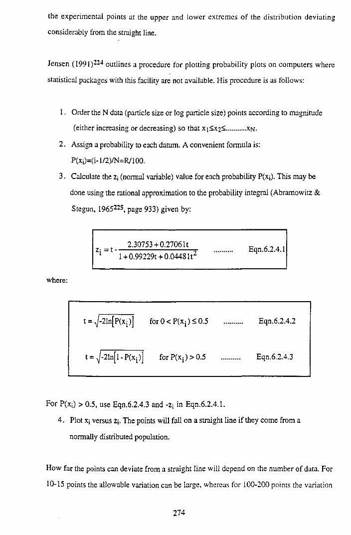
the experimental points at the upper and lower extremes of the distribution deviating

considerably from the straight line.

Jensen (1991)224 outlines a procedure for plotting probability plots on computers where

statistical packages with this facility are not available. His procedure is as follows:

1. Order the N data (particle size or log particle size) points according to magnitude

(either increasing or decreasing) so that xi<X2^ .......... xn-

2. Assign a probability to each datum. A convenient formula is:

P(xi)=(i-l/2)/N=R/100.

3. Calculate the Zj (normal variable) value for each probability P(xj). This may be

done using the rational approximation to the probability integral (Abramowitz &

Stegun, 196522S, page 933) given by:

where:

2.30753+ 0.2706 It 1 _ l + 0.99229t + 0.0448 I t2

Eqn.6.2.4.1

t = ^y~21n[P(xi )] fo r0 < P (x i )< 0 .5 .......... Eqn.6.2.4.2

t = ^-21n[l-P(Xi)] for P(Xj) > 0.5 .......... Eqn.6.2.4.3

For P(xO > 0.5, use Eqn.6.2.4.3 and -z, in Eqn.6.2.4.1.

4. Plot x; versus z;. The points will fall on a straight line if they come from a

normally distributed population.

How far the points can deviate from a straight line will depend on the number of data. For

10-15 points the allowable variation can be large, whereas for 100-200 points the variation

274

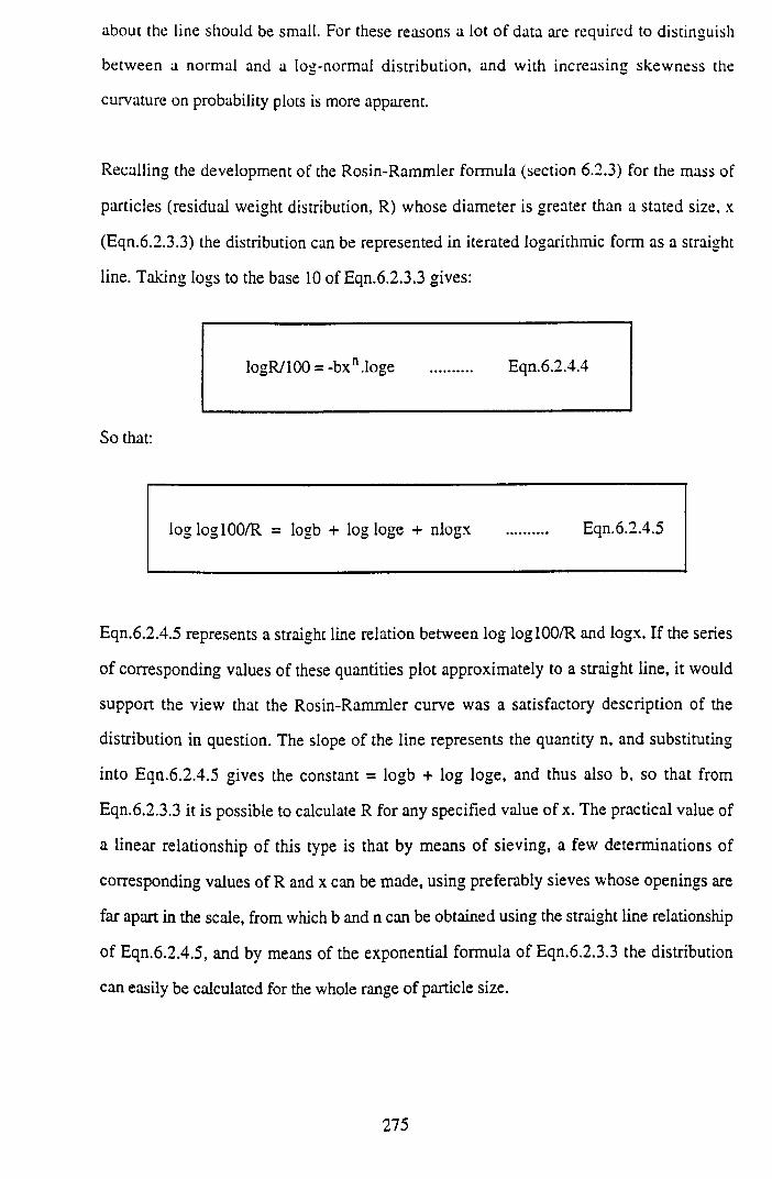
about the line should be small. For these reasons a lot of data are required to distinguish

between a normal and a log-normal distribution, and with increasing skewness the

curvature on probability plots is more apparent.

Recalling the development of the Rosin-Rammler formula (section 6.2.3) for the mass of

particles (residual weight distribution, R) whose diameter is greater than a stated size, x

(Eqn.6.2.3.3) the distribution can be represented in iterated logarithmic form as a straight

line. Taking logs to the base 10 of Eqn.6.2.3.3 gives:

logR/100 = -bxn.loge .......... Eqn.6.2.4.4

So that:

logloglOO/R = logb + log loge + nlogx .......... Eqn.6.2.4.5

Eqn.6.2.4.5 represents a straight line relation between log loglOO/R and logx. If the series

of corresponding values of these quantities plot approximately to a straight line, it would

support the view that the Rosin-Rammler curve was a satisfactory description of the

distribution in question. The slope of the line represents the quantity n, and substituting

into Eqn.6.2.4.5 gives the constant = logb + log loge, and thus also b, so that from

Eqn.6.2.3.3 it is possible to calculate R for any specified value of x. The practical value of

a linear relationship of this type is that by means of sieving, a few determinations of

corresponding values of R and x can be made, using preferably sieves whose openings are

far apart in the scale, from which b and n can be obtained using the straight line relationship

of Eqn.6.2.4.5, and by means of the exponential formula of Eqn.6.2.3.3 the distribution

can easily be calculated for the whole range of particle size.

275

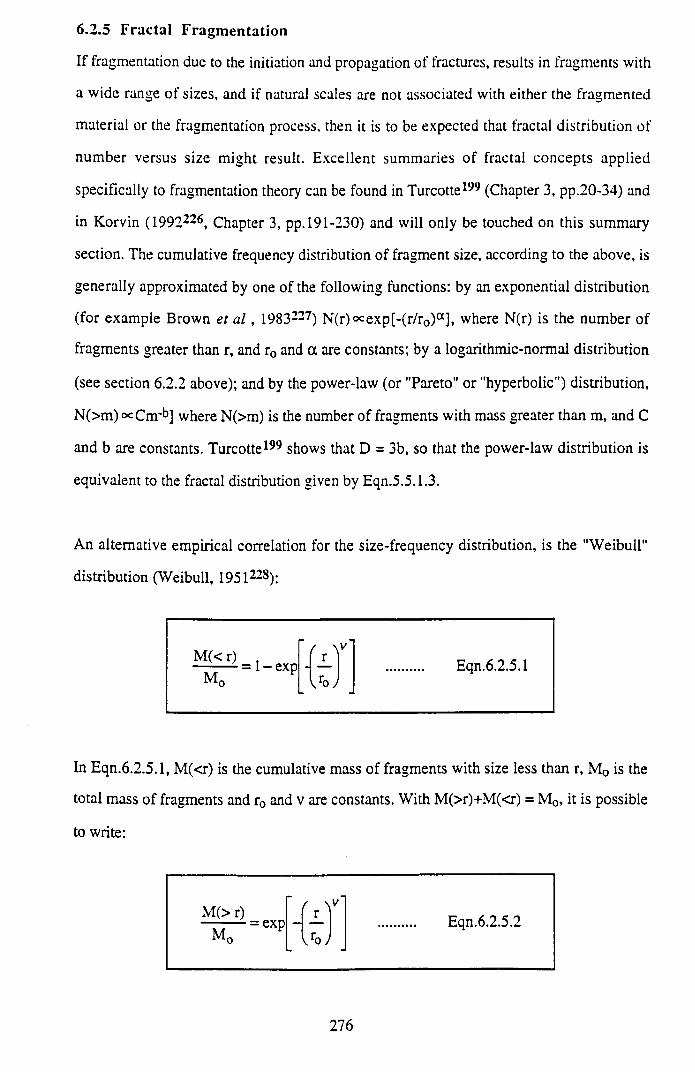
6.2.5 Fractal Fragmentation

If fragmentation due to the initiation and propagation of fractures, results in fragments with

a wide range of sizes, and if natural scales are not associated with either the fragmented

material or the fragmentation process, then it is to be expected that fractal distribution of

number versus size might result. Excellent summaries of fractal concepts applied

specifically to fragmentation theory can be found in Turcotte199 (Chapter 3, pp.20-34) and

in Korvin (1992226, Chapter 3, pp. 191-230) and will only be touched on this summary

section. The cumulative frequency distribution of fragment size, according to the above, is

generally approximated by one of the following functions: by an exponential distribution

(for example Brown et a l , 1983227) N(r)«=exp[-(r/r0)a ], where N(r) is the number of

fragments greater than r, and r0 and a are constants; by a logarithmic-normal distribution

(see section 6.2.2 above); and by the power-law (or "Pareto" or "hyperbolic") distribution,

N(>m)ocCm'b] where N(>m) is the number of fragments with mass greater than m, and C

and b are constants. Turcotte199 shows that D = 3b, so that the power-law distribution is

equivalent to the fractal distribution given by Eqn.5.5.1.3.

An alternative empirical correlation for the size-frequency distribution, is the "Weibull"

distribution (Weibull, 1951228):

M(< r) M 0

1 -ex pv ro y

Eqn.6.2.5.1

In Eqn.6.2.5.1, M(<r) is the cumulative mass of fragments with size less than r, M0 is the

total mass of fragments and r0 and v are constants. With M(>r)+M(<r) = M0, it is possible

to write:

M(> r) M0

= exp f-T<r0>

Eqn.6.2.5.2

276

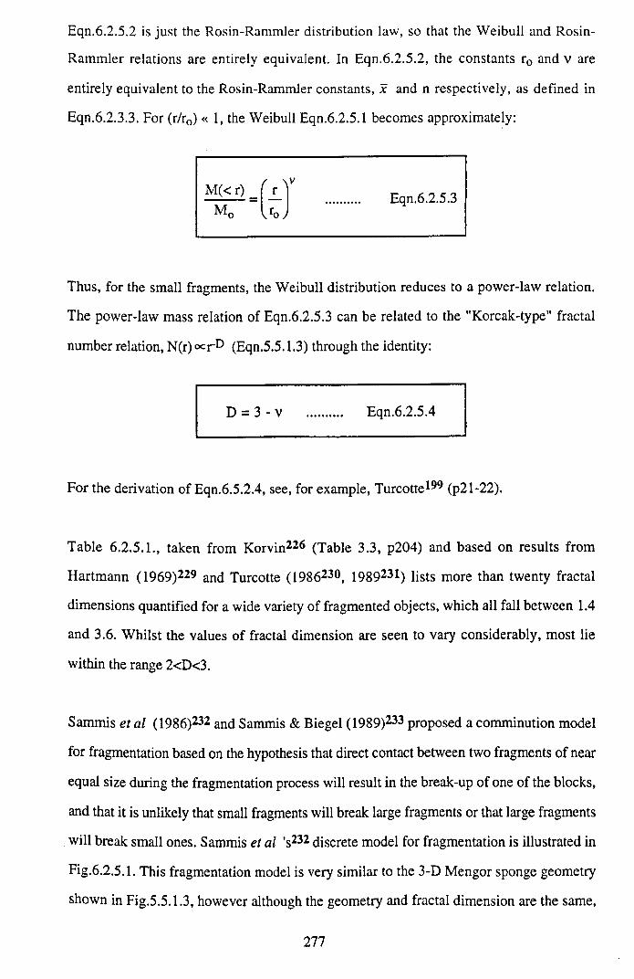
Eqn.6.2.5.2 is just the Rosin-Rammler distribution law, so that the Weibull and Rosin-

Rammler relations are entirely equivalent. In Eqn.6.2.5.2, the constants rQ and v are

entirely equivalent to the Rosin-Rammler constants, x and n respectively, as defined in

Eqn.6.2.3.3. For (r/rQ) « 1, the Weibull Eqn.6.2.5.1 becomes approximately:

M(< r) M 0 v ro y

Eqn.6.2.5.3

Thus, for the small fragments, the Weibull distribution reduces to a power-law relation.

The power-law mass relation of Eqn.6.2.5.3 can be related to the "Korcak-type" fractal

number relation, N(r) <^rD (Eqn.5.5.1.3) through the identity:

D = 3 - v .......... Eqn.6.2.5.4

For the derivation of Eqn.6.5.2.4, see, for example, Turcotte199 (p21-22).

Table 6.2.5.1., taken from Korvin226 (Table 3.3, p204) and based on results from

Hartmann (1969)229 and Turcotte (1986230, 1989231) lists more than twenty fractal

dimensions quantified for a wide variety of fragmented objects, which all fall between 1.4

and 3.6. Whilst the values of fractal dimension are seen to vary considerably, most lie

within the range 2<D<3.

Sammis et al (1986)232 and Sammis & Biegel (1989)233 proposed a comminution model

for fragmentation based on the hypothesis that direct contact between two fragments of near

equal size during the fragmentation process will result in the break-up of one of the blocks,

and that it is unlikely that small fragments will break large fragments or that large fragments

will break small ones. Sammis et a l 's232 discrete model for fragmentation is illustrated in

Fig.6.2.5.1. This fragmentation model is very similar to the 3-D Mengor sponge geometry

shown in Fig.5.5.1.3, however although the geometry and fractal dimension are the same,

277

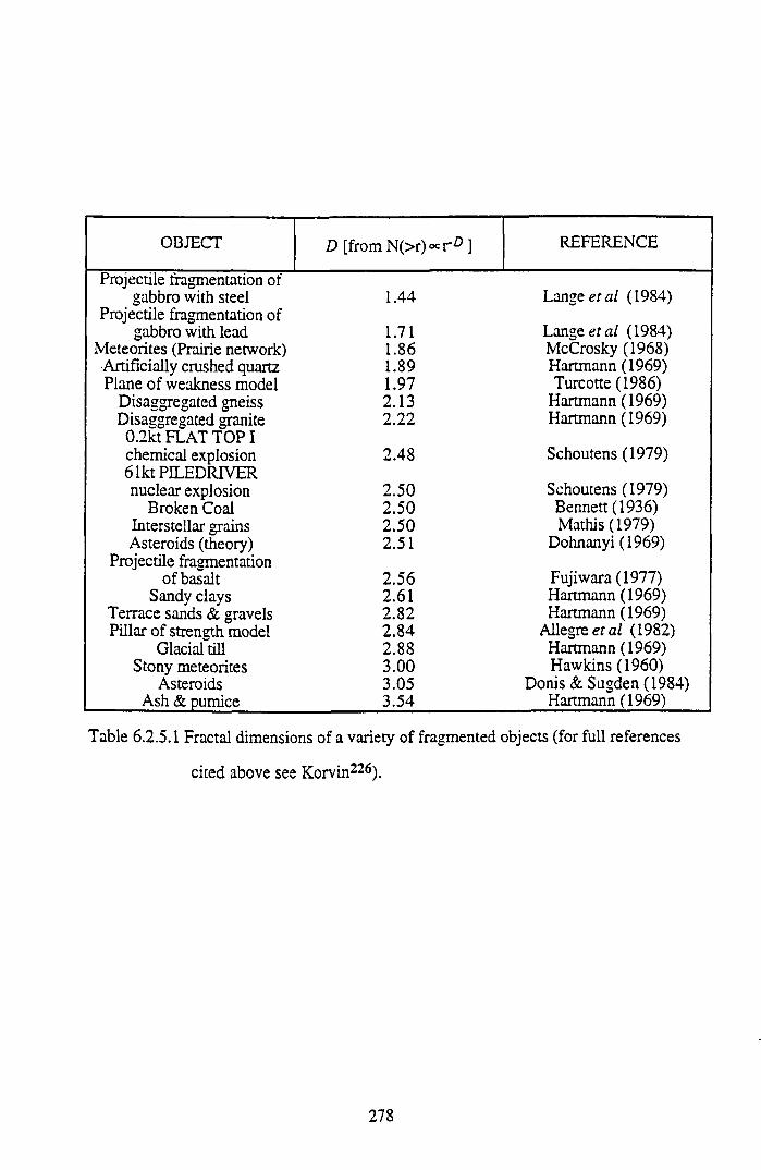
OBJECT D [from N(>r) °= r D ] REFERENCE

Projectile fragmentation ofgabbro with steel 1.44 Lange et al (1984)

Projectile fragmentation ofgabbro with lead 1.71 Lange et al (1984)

Meteorites (Prairie network) 1.86 McCrosky (1968)Artificially crushed quartz 1.89 Hartmann (1969)Plane of weakness model 1.97 Turcotte (1986)

Disaggregated gneiss 2.13 Hartmann ( 1969)Disaggregated granite 2.22 Hartmann (1969)

0.2kt FLAT TOP Ichemical explosion 2.48 Schoutens (1979)61ktPHEDRIVERnuclear explosion 2.50 Schoutens (1979)

Broken Coal 2.50 Bennett (1936)Interstellar grains 2.50 Mathis (1979)Asteroids (theory) 2.51 Dohnanyi (1969)

Projectile fragmentationof basalt 2.56 Fujiwara (1977)

Sandy clays 2.61 Hartmann (1969)Terrace sands & gravels 2.82 Hartmann (1969)Pillar of strength model 2.84 Allegre et al (1982)

Glacial till 2.88 Hartmann (1969)Stony meteorites 3.00 Hawkins (1960)

Asteroids 3.05 Donis & Sugden (1984)Ash & pumice 3.54 Hartmann (1969)

Table 6.2.5.1 Fractal dimensions of a variety of fragmented objects (for full references

cited above see Korvin226).

278

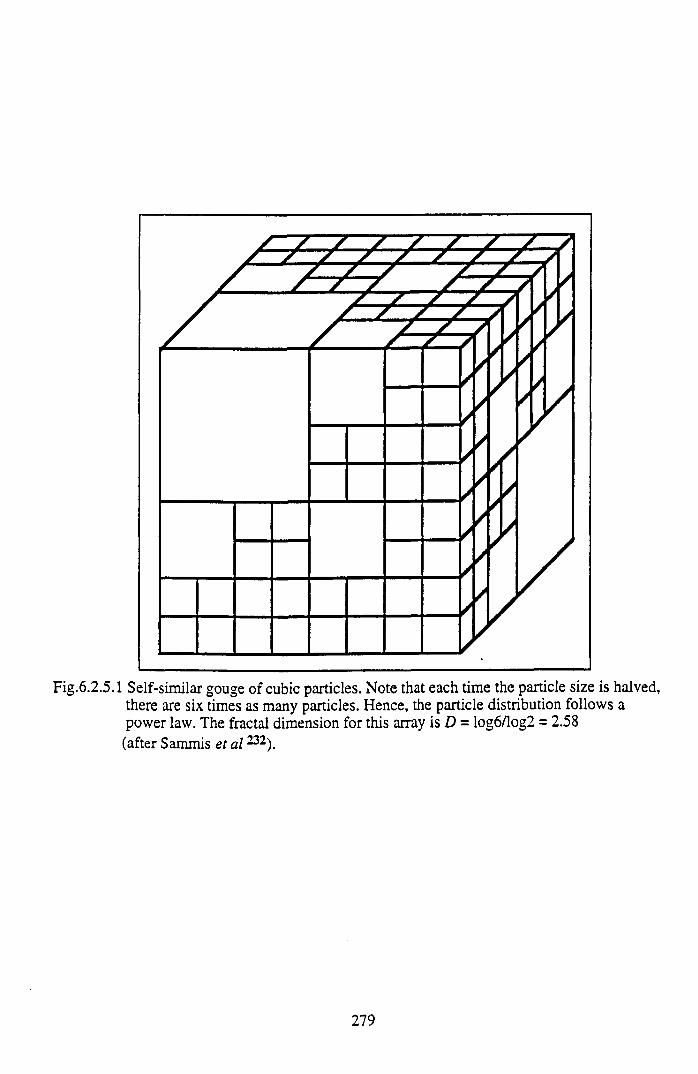
Fig.6.2.5.1 Self-similar gouge of cubic particles. Note that each time the panicle size is halved, there are six times as many panicles. Hence, the particle distribution follows a power law. The fractal dimension for this array is D - log6/log2 = 2.58 (after Sammis et a l232).

279

the concepts of the two models are quite different - in the former the models are for porous

configurations, whereas in the latter fragmentation is considered in which some blocks are

retained at each scale, but others are fragmented. In Fig.6.2.5.1, two diagonally opposed

blocks are retained at each scale, so that no two fragmented blocks of equal size are in

direct contact with each other. For this array of cubes, each decrease in particle size by a

factor of 1/2 corresponds to an increase in the number of particles by a factor of six, so that

from Eqn.5.5.1.2, this gives a fractal dimension, D = (log6)/(log2) = 2.5850. Sammis et al

(1987)234 measured the particle-size distribution over the range 5microns to 4mm, of a

natural fault gouge from the Lopez Canyon Fault in the San Gabriel Mountains of Southern

California, using optical and electron microscopy, and found the fractal dimension to be

1.60±0.11 in 2-D cross-section, and thus 2.60+0.11 in an isotropic 3-D volume.

However, Sammisei al 232 pointed out that when the cumulative volume fraction for this

self-similar distribution is plotted on log-normal probability paper, it is evident that the finer

fractions might be interpreted as log-normal (that is as a straight-line) thus making it

impossible to distinguish, for this particular particle-size range, between a log-normal and a

self-similar distribution.

6.3 EXPERIMENTAL SIZE DISTRIBUTION DETERMINATION

Grain-size distribution has been traditionally characterised in the hydrocarbon industry

using sieve analysis, settling tube velocity measurements and thin-section grain-size

analysis. However these methods are relatively time-consuming and do not permit detailed

classification of the silt and clay size fractions. Accordingly, existing laser optics

technology, initially developed for the powder industry, has been utilised to analyse the

experimental fault gouge particle distributions. This laser technology offers a considerable

extension to the common range of particle size measurement, size determination is rapid,

and the data are reproducible. Laser sizing is readily adapted to distribution analysis of

friable and unconsolidated sediments, and so is ideal for the experimental shear debris

samples which are, unlike much natural gouge material, non-indurated (unhardened). As

far as the author is aware, the only published example of the application of extended range

particle size analysis using laser diffraction technology within the petroleum industry, is

that of Griffin (1991)17 who showed favourable comparison between laser optics data with

280

sieve analysis and settling tube analysis over traditional measurement ranges, with the clay

size fraction comparing favourably with clay content determined by X-ray diffraction.

Griffin highlighted the potential insights offered by such extended range data in well

completion strategies (quantification of sand production and potentially mobile fines)

sedimentology (determination of sediment uniformity) and log evaluation (determination of

Vshale on cores).

As far as is known, the first published example of laser sizing technology being applied

directly to fault gouge distributions, is that of Crawford et al (1994)236 following from

analysis of the direct shear experimental debris detailed in section 6.4 below. Laser sizing

theory, equipment specifics and experimental methodology are described in section 6.3.2

below, whilst more common sieve analyses are used for comparative purposes (sieving

technique outlined in section 6.3.1) to contrast with the broad range laser sizing results.

6.3.1 Sieving

Sieving is one of the simplest methods of determining particle size distributions, and is

generally overlooked when carrying out fundamental research, which is unfortunate as it

can be a very accurate technique. Sieving analysis applies to a range of grain sizes from

very large grains (typically <1000microns) down to grains of about 0.05mm (50microns).

With smaller grains the method cannot be applied, as it is impossible to produce sieve

meshes fine enough for this purpose, and also due to the fact that for very small grains, the

force of gravity is not great enough to overcome the resistance of grains to fall, resulting

from grain adherence to one another and to the sieve cloth. Fortunately, the size of sieve

screen openings have been standardised. Most sieves which are used for particle size

determination have square openings, although circular, rectangular and even slit openings

are available. In the USA the ‘Tyler” standard sieve series is used, based on the size of

openings in wire cloth having 200 openings per linear inch (200-mesh). In the Tyler series,

the openings of successive sieves are at the fixed ratio of V2, so that the areas of the

openings of each sieve are double those o f the next finer sieve. The British Standards

Institution in 1932 adopted a sieve series known as the British Standard Sieve Series. The

ration is the same as for the Tyler series, and the openings are nearly the same (the slight

281

differences being due to differences between U.S. and British wire). The sieve size

openings of the Tyler and B.S. series are compared in Table 6.3.1.1 (those used in the

present study being marked with an asterisk).

The sieving analysis relies on putting the substance concerned through a number of sieves

of successively smaller mesh size, and determining the weight fraction which has passed

each sieve, or which passes one sieve and is retained on the next smaller size. According to

whether only the weight undersize (or weight oversize) fraction is determined, or the

fraction passed and retained by two neighbouring sieves, the distribution of pardcle size is

obtained in the form of either the weight cumulative or the weight frequency distribution.

The errors specific to analysis by sieving arise out of the fact that the examination with

regard to size is here performed simultaneously on a very great mass of particles, instead of

individually as in the case of microscopic examination. Thus whether a particle will pass

the sieve aperture depends not only on its dimensions in relation to those of the sieve

aperture, but on many other factors including the size of the other particles and their

quantity, whether it has free access to a given aperture and how it presents itself to the

aperture, and the time of sieving during which such access may be gained, all such factors

resulting in the particle only having a certain probability of passing the aperture in a given

time.

6.3.2 Laser Sizing

The laser device used in the determinations on experimental fault gouge presented in this

chapter is a Mastersizer high resolution 0.1-600microns particle size analyser supplied by

©M alvern Instruments Ltd, and the equipment design, capabilities and operating

procedures detailed here are largely drawn from their Instruction Manual237. The system

utilises composite laser light diffraction patterns produced by the dispersed particles to

compute size distributions. Fig.6.3.2.1 is a schematic representation of the device. In

essence, the laser light scattering sizer comprises a sample recirculating system which

transports and presents the dispersed sample material to the measurement zone, an optical

measurement unit that forms the basic particle size sensor, and a computer that manages the

measurement and performs results analyses and presentation.

282

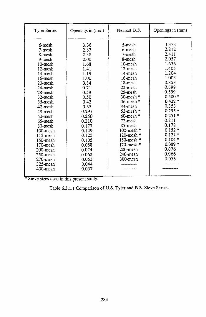
Tyler Series Openings in (mm) Nearest B.S. Openings in (mm)

6-mesh 3.36 5-mesh 3.3537-mesh 2.83 6-mesh 2.8128-mesh 2.38 7-mesh 2.4119-mesh 2.00 8-mesh 2.05710-mesh 1.68 10-mesh 1.67612-mesh 1.41 12-mesh 1.40514-mesh 1.19 14-mesh 1.20416-mesh 1.00 16-mesh 1.00320-mesh 0.84 18-mesh 0.85324-mesh 0.71 22-mesh 0.69928-mesh 0.59 25-mesh 0.59932-mesh 0.50 30-mesh * 0.500 *35-mesh 0.42 3 6-mesh * 0.422 *42-mesh 0.35 44-mesh 0.35348-mesh 0.297 52-mesh * 0.295 *60-mesh 0.250 60-mesh * 0.251 *65-mesh 0.210 72-mesh 0.21180-mesh 0.177 85-mesh 0.178100-mesh 0.149 100-mesh * 0.152 *115-mesh 0.125 120-mesh * 0.124*150-mesh 0.105 150-mesh * 0.104*170-mesh 0.088 170-mesh * 0.089 *200-mesh 0.074 200-mesh 0.076250-mesh 0.062 240-mesh 0.066270-mesh 0.053 300-mesh 0.053325-mesh 0.044 —

400-mesh 0.037

* Sieve sizes used in this present study.

Table 6.3.1.1 Comparison of U.S. Tyler and B.S. Sieve Series.

283

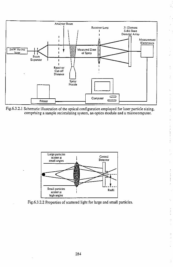
Fig.6.3.2.1 Schematic illustration of the optical configuration employed for laser particle sizing, comprising a sample recirculating system, an optics module and a microcomputer.

Fig.6.3.2.2 Properties of scattered light for large and small particles.

284

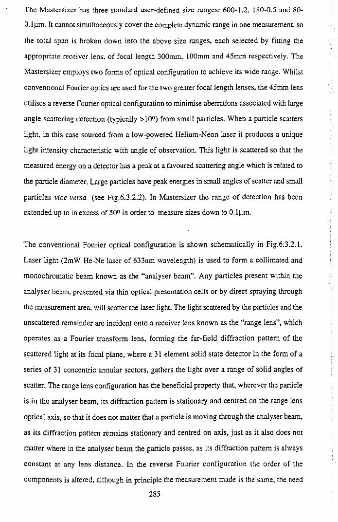
The Mastersizer has three standard user-defined size ranges: 600-1.2, 180-0.5 and 80-

0 .1p.m. It cannot simultaneously cover the complete dynamic range in one measurement, so

the total span is broken down into the above size ranges, each selected by fitting the

appropriate receiver lens, of focal length 300mm, 100mm and 45mm respectively. The

Mastersizer employs two forms of optical configuration to achieve its wide range. Whilst

conventional Fourier optics are used for the two greater focal length lenses, the 45 mm lens

utilises a reverse Fourier optical configuration to minimise aberrations associated with large

angle scattering detection (typically >10°) from small particles. When a particle scatters

light, in this case sourced from a low-powered Helium-Neon laser it produces a unique

light intensity characteristic with angle of observation. This light is scattered so that the

measured energy on a detector has a peak at a favoured scattering angle which is related to

the particle diameter. Large particles have peak energies in small angles of scatter and small

particles vice versa (see Fig.6.3.2.2). In Mastersizer the range o f detection has been

extended up to in excess of 50° in order to measure sizes down to 0.1p.m.

The conventional Fourier optical configuration is shown schematically in Fig.6.3.2.1.

Laser light (2mW He-Ne laser of 633nm wavelength) is used to form a collimated and

monochromatic beam known as the “analyser beam”. Any particles present within the

analyser beam, presented via thin optical presentation cells or by direct spraying through

the measurement area, will scatter the laser light. The light scattered by the particles and the

unscattered remainder are incident onto a receiver lens known as the “range lens”, which

operates as a Fourier transform lens, forming the far-field diffraction pattern of the

scattered light at its focal plane, where a 31 element solid state detector in the form of a

series of 31 concentric annular sectors, gathers the light over a range of solid angles of

scatter. The range lens configuration has the beneficial property that, wherever the particle

is in the analyser beam, its diffraction pattern is stationary and centred on the range lens

optical axis, so that it does not matter that a particle is moving through the analyser beam,

as its diffraction pattern remains stationary and centred on axis, just as it also does not

matter where in the analyser beam the particle passes, as its diffraction pattern is always

constant at any lens distance. In the reverse Fourier configuration the order of the

components is altered, although in principle the measurement made is the same, the need

285

for the new configuration arising from the necessity to measure scattering at much higher

angles than is feasible using the conventional method. Despite the modified optics, the

diffraction pattern received by the detector still remains stationary and coaxial within the

laser axis, regardless of particle movement.

The Malvern Mastersizer allows 3 particle size ranges with an overall span of 6000:1 to be

accessed through choice of the range lens and optical configuration, necessitating the use of

different optical theories to model the scattering. For scattering angles of 0.01-15°

corresponding to a size range of 2p.m and upwards, the scattering angle is largely

independent of the optical properties of the material and the medium of suspension, and is

caused by the diffraction of light around the particle. Light that couples into the particle is

absorbed in all common cases and can be ignored, the "Fraunhofer" scattering theory

(which assumes the particles scatter light like discs of the same diameter) proving adequate

for modelling, without any requirements with regard to the powders’ optical properties.

However, for a detection range which has been extended up to >50° in order to measure

down to 0.1 (im, the scattering from such small particles at such high angles becomes

heavily dependent on the optical properties of the material, necessitating use of the "Mie"

theory model of light scattering. Mie theory is an exact solution to the Maxwell’s equations

for the case of a spherical particle, providing a complete description of the light scattering

from optically homogeneous spheres, and requires assumptions regarding the optical nature

of the particles. The optical constants that determine the scattering behaviour can be reduced

to two, the differential refractive index between dispersant and particle, and the particle

absorption, which can be set in the Mastersizer software using a four character code. The

Fraunhofer scattering model is fully encompassed by the Mie theory, and fully agrees with

it in the applicable range.

The time-averaged diffraction pattern shape is a convolution of the contributions of all of

the particles of the composite sample. Signals from the measurment windows are

econvolved into a multi-channnel histogram of the particle size distribution by a complex

algorithm. The algorithms used to calculate particle size distribution from composite

diffraction patterns are manufacturer dependent and proprietary, however from

286

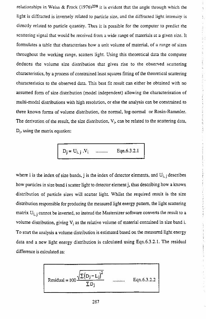
relationships in Weiss & Frock (1976)238 it is evident that the angle through which the

light is diffracted is inversely related to particle size, and the diffracted light intensity is

directly related to particle quantity. Thus it is possible for the computer to predict the

scattering signal that would be received from a wide range of materials at a given size. It

formulates a table that characterises how a unit volume of material, of a range of sizes

throughout the working range, scatters light. Using this theoretical data the computer

deduces the volume size distribution that gives rise to the observed scattering

characteristics, by a process of constrained least squares fitting of the theoretical scattering

characteristics to the observed data. This best fit result can either be obtained with no

assumed form of size distribution (model independent) allowing the characterisation of

multi-modal distributions with high resolution, or else the analysis can be constrained to

three known forms of volume distribution, the normal, log-normal or Rosin-Rammler.

The derivation of the result, the size distribution, V;, can be related to the scattering data,

D j , using the matrix equation:

where i is the index of size bands, j is the index of detector elements, and Ui, j describes

how panicles in size band i scatter light to detector element j, thus describing how a known

distribution of particle sizes will scatter light. Whilst the required result is the size

distribution responsible for producing the measured light energy pattern, the light scattering

matrix Uit j cannot be inverted, so instead the Mastersizer software converts the result to a

volume distribution, giving Vj as the relative volume of material contained in size band i.

To start the analysis a volume distribution is estimated based on the measured light energy

data and a new light energy distribution is calculated using Eqn.6.3.2.1. The residual

difference is calculated as:

Eqn.6.3.2.1

Eqn.6.3.2.2

287

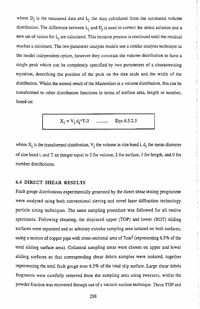
where Dj is the measured data and Lj the data calculated from the estimated volume

distribution. The difference between Lj and Dj is used to correct the initial solution and a

new set of values for Lj are calculated. This iterative process is continued until the residual

reaches a minimum. The two parameter analysis models use a similar analysis technique as

the model independent option, however they constrain the volume distribution to have a

single peak which can be completely specified by two parameters of a characterising

equation, describing the position of the peak on the size scale and the width of the

distribution. Whilst the natural result of the Mastersizer is a volume distribution, this can be

transformed to other distribution functions in terms of surface area, length or number,

based on:

Xj = Vj.djAT-3 .......... Eqn.6.3.2.3

where Xj is the transformed distribution, Vj the volume in size band i, dj the mean diameter

of size band i, and T an integer equal to 3 for volume, 2 for surface, 1 for length, and 0 for

number distributions.

6.4 D IR EC T SH EA R RESULTS

Fault gouge distributions experimentally generated by the direct shear testing programme

were analysed using both conventional sieving and novel laser diffraction technology

particle sizing techniques. The same sampling procedure was followed for all twelve

specimens. Following shearing, the displaced upper (TOP) and lower (BOT) sliding

surfaces were separated and an arbitrary circular sampling area isolated on both surfaces,

using a section of copper pipe with cross-sectional area of 7cm^ (representing 6.5% of the

total sliding surface area). Collateral sampling areas were chosen on upper and lower

sliding surfaces so that corresponding shear debris samples were isolated, together

representing the total fault gouge over 6.5% of the total slip surface. Large shear debris

fragments were carefully removed from the sampling area using tweezers, whilst the

powder fraction was recovered through use of a vacuum suction technique. These TOP and

288

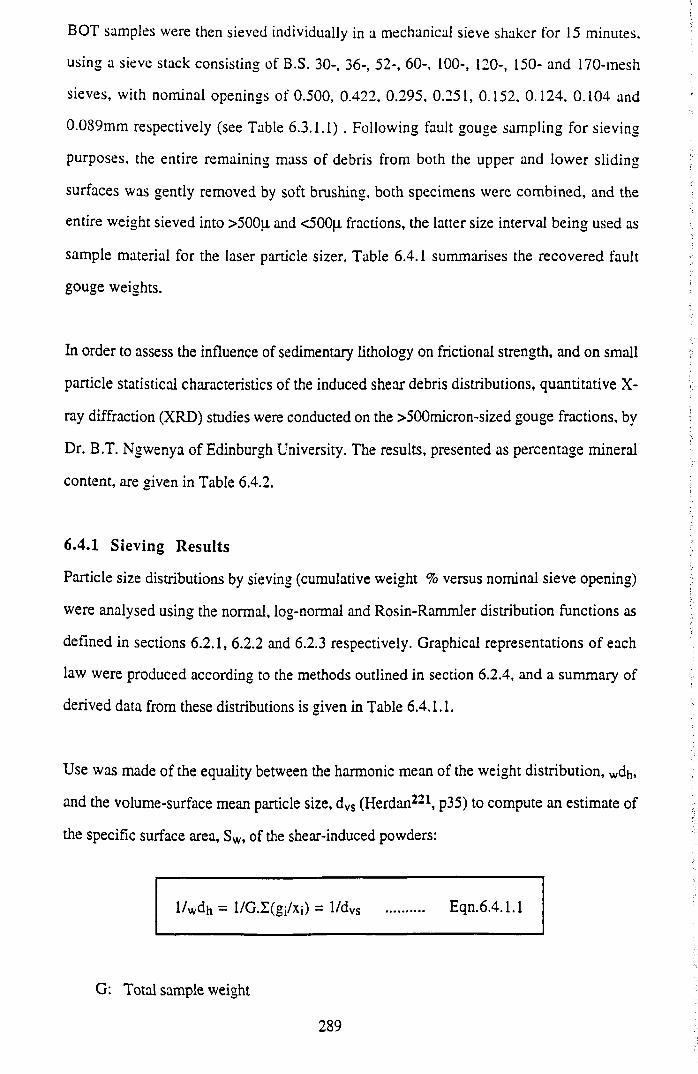
BOT samples were then sieved individually in a mechanical sieve shaker for 15 minutes,

using a sieve stack consisting of B.S. 30-, 36-, 52-, 60-, 100-, 120-, 150- and 170-mesh

sieves, with nominal openings of 0.500, 0.422. 0.295, 0.251, 0.152, 0.124, 0.104 and

0.089mm respectively (see Table 6.3.1.1) . Following fault gouge sampling for sieving

purposes, the entire remaining mass of debris from both the upper and lower sliding

surfaces was gently removed by soft brushing, both specimens were combined, and the

entire weight sieved into >500(i and <500(1 fractions, the latter size interval being used as

sample material for the laser particle sizer. Table 6.4.1 summarises the recovered fault

gouge weights.

In order to assess the influence of sedimentary lithology on frictional strength, and on small

particle statistical characteristics of the induced shear debris distributions, quantitative X-

ray diffraction (XRD) studies were conducted on the >500micron-sized gouge fractions, by

Dr. B.T. Ngwenya of Edinburgh University. The results, presented as percentage mineral

content, are given in Table 6.4.2.

6.4.1 Sieving R esu lts

Particle size distributions by sieving (cumulative weight % versus nominal sieve opening)

were analysed using the normal, log-normal and Rosin-Rammler distribution functions as

defined in sections 6.2.1, 6.2.2 and 6.2.3 respectively. Graphical representations of each

law were produced according to the methods outlined in section 6.2.4, and a summary of

derived data from these distributions is given in Table 6.4.1.1.

Use was made of the equality between the harmonic mean of the weight distribution, wdh,

and the volume-surface mean particle size, dvs (Herdan221, p35) to compute an estimate of

the specific surface area, Sw, of the shear-induced powders:

l / wdh = l/G .I(gi/xi) = 1/dvs .......... Eqn.6.4.1.1

G: Total sample weight

289

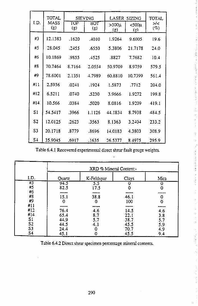
I.D.TOTALMASS

(g)

SIEVING LASER SIZING TOTAL>/<(%)

TOP(g)

BOT(g)

>500^(g)

<500(i(?)

#3 12.1383 .1620 .4010 1.9264 9.6005 19.6

#5 28.045 .2455 .6550 5.3806 21.7178 24.0

#6 10.1869 .9855 .4525 .8827 7.7682 10.4

#8 70.7464 8.7164 2.0554 50.9709 8.9759 579.5

#9 78.6001 2.1351 4.7989 60.8810 10.7399 561.4

#11 2.5936 .0241 .1924 1.5873 .7712 204.0

#12 6.5211 .0740 .5230 3.9666 1.9272 199.8

#14 10.566 .0384 .5020 8.0816 1.9209 419.1

SI 54.5417 .3966 1.1126 44.1834 8.7938 484.5

S2 12.0125 .2623 .3563 8.1363 3.2404 233.2

S3 20.1718 .8779 .8696 14.0183 4.3803 308.9

S4 35.9045 .6917 .1635 26.5377 8.4975 295.9

Table 6.4.1 Recovered experimental direct shear fault gouge weights.

I.D.

XRD % Mineral Content:-

Quartz K-Feldspar Clavs Mica#3 94.5 5.5 0 0#5#6

82.5 17.5 0 0

#8 15.1 38.8 46.1 0#9 0 0 100 0

#11 ..... .....#12 76.4 4.6 14.5 4.6#14 65.4 8.7 22.1 3.8SI 44.9 5.7 38.7 5.7S2 44.5 4.1 45.5 5.9S3 24.4 0 70.7 4.9S4 45.1 0 45.5 9.4

Table 6.4.2 Direct shear specimen percentage mineral contents.

290

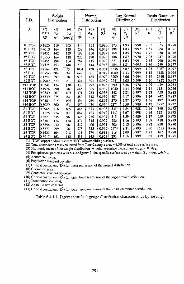
I.D.Weight

DistributionNormal

DistributionLog-NormalDistribution

Rosin-RammierDistribution

(l) (2) (3) (4) (5) (6) (7) (8) (9) (10) (11) (12) 03)Mass dvs Sw X CTn-l R2 X (T a„ R2 n X R2(g) W (cm2/g) (u) (d) w W W

#3 TOP 0.1620 219 103 314 158 0.980 273 1.93 0.990 2.03 355 0.998#3 BOT 0.4010 164 138 238 146 0.972 198 1.83 0.992 1.87 268 0.991#5 TOP 0.2455 142 159 198 150 0.927 168 1.85 0.994 1.72 230 0.976#5 BOT 0.6550 164 138 220 120 0.995 184 1.67 0.970 2.05 247 0.996#6 TOP 0.9855 198 114 264 115 0.979 221 1.63 0.991 2.53 290 0.989#6 BOT 0.4525 153 148 220 144 0.943 184 1.81 0.995 1.86 249 0.977#8 TOP 8.7164 428 53 1031 428 0.954 5236 5.87 0.999 1.25 3067 0.997#8 BOT 2.0554 304 74 649 361 0.949 1080 4.43 0.999 1.15 1158 0.995#9 TOP 2.1351 392 58 916 485 0.920 3709 6.06 0.994 1.14 2610 0.987#9 BOT 4.7989 372 61 824 391 0.957 2241 5.05 0.999 1.20 1852 0.997

#11 TOP 0.0241 174 130 333 297 0.878 290 3.28 0.978 1.09 419 0.953#11 BOT 0.1924 290 78 645 365 0.932 1050 4.44 0.996 1.14 1131 0.986#12 TOP 0.0740 207 109 371 252 0.936 342 2.81 0.997 1.33 458 0.983#12 BOT 0.5230 275 82 580 348 0.939 807 4.17 0.996 1.14 942 0.987#14 TOP 0.0384 215 105 394 264 0.867 370 2.87 0.973 1.36 482 0.943#14 BOT 0.5020 360 63 850 424 0.910 2371 5.59 0.989 1.12 1972 0.977SI TOP 0.3966 216 105 485 373 0.908 539 4.54 0.988 0.96 740 0.973SI BOT 1.1126 274 83 664 423 0.942 1141 5.67 0.998 0.94 1331 0.993S2 TOP 0.2623 235 96 326 275 0.907 515 3.59 0.989 1.17 659 0.973S2 BOT 0.3563 174 130 474 315 0.977 286 3.16 0.995 1.09 418 0.999S3 TOP 0.8696 232 98 549 400 0.931 706 5.13 0.996 0.92 938 0.990S3 BOT 0.8779 299 76 858 535 0.919 2474 8.81 0.993 0.80 2553 0.986S4 TOP 0.1635 104 218 118 174 0.988 119 2.09 0.987 1.21 162 0.998S4BOT 0.6917 162 140 333 345 0.953 293 4.16 0.999 0.88 459 0.995

(1) "TOP"=upper sliding surface; "BOT"=lower sliding surface.(2) Total shear debris mass collected from 7cmA2 sample area = 6.5% of total slip surface area.(3) Harmonic mean of the weight distribution = volume-surface mean diameter, wdj, s dVs.(4) For spherical particles with p = 2.65gcmA-3, the specific surface area by weight, Sw = 6/p. wd(,A-l.(5) Arithmetic mean.(6) Population standard deviation.(7) Critical coefficient (R2) for linear regression of the normal distribution.(8) Geometric mean.(9) Geometric standard deviation.

(10) Critical coefficient (R2) for logarithmic regression of the log-normal distribution.(11) Distribution constant.(12) Absolute size constant.(13) Critical coefficient (R2) for logarithmic regression of the Rosin-Rammler distribution.

Table 6.4.1.1. Direct shear fault gouge distribution characteristics by sieving.

291

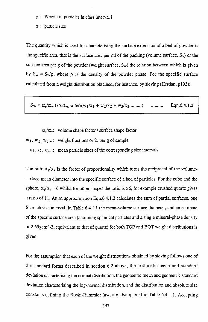
g;: Weight of particles in class interval i

x\: particle size

The quantity which is used for characterising the surface extension of a bed of powder is

the specific area, that is the surface area per ml of the packing (volume surface, Sv) or the

surface area per g of the powder (weight surface, Sw) the relation between which is given

by Sw = Sv/p, where p is the density of the powder phase. For the specific surface

calculated from a weight distribution obtained, for instance, by sieving (Herdan, p 193):

Sw = a s/ a v.l/p .d vs = 6/p(w i/xi + W2/X2 + W3/X3.......... ) .......... Eqn.6.4.1.2

a s/ a v: volume shape factor / surface shape factor

w 1, W 2 , W 3 ...: weight fractions or % per g of sample

x 1 . x 2 > X 3 ...: mean particle sizes of the corresponding size intervals

The ratio a s/ a v is the factor of proportionality which turns the reciprocal of the volume-

surface mean diameter into the specific surface of a bed of particles. For the cube and the

sphere, a s/a v = 6 whilst for other shapes the ratio is >6, for example crushed quartz gives

a ratio of 11. As an approximation Eqn.6.4.1.2 calculates the sum of partial surfaces, one

for each size interval. In Table 6.4.1.1 the mean-volume surface diameter, and an estimate

of the specific surface area (assuming spherical particles and a single mineral-phase density

of 2.65gcmA-3, equivalent to that of quartz) for both TOP and BOT weight distributions is

given.

For the assumption that each of the weight distributions obtained by sieving follows one of

the standard forms described in section 6.2 above, the arithmetic mean and standard

deviation characterising the normal distribution, the geometric mean and geometric standard

deviation characterising the log-normal distribution, and the distribution and absolute size

constants defining the Rosin-Rammler law, are also quoted in Table 6 .4 .1 . 1 . Accepting

292

that the straight line of the graph is some evidence, even though no strict mathematical

proof, that the distribution is governed by the normal, log-normal or Rosin-Rammler laws,

critical coefficients, R- (where R = correlation coefficient) are tabulated in Table 6.4.1.1

for regression fits to the three distribution functions. Visual inspection of the plots shows a

systematic curvature to all of the normal distributions, which also possess the lowest of the

critical coefficients, suggesting that this is not a valid law for particle size distributions

obtained by direct shear. Visual inspection of the log-normal and power-law distributions

show much closer approximations to linearity (although some are still visibly curved, for

example the Rosin-Rammler plots of specimens #11, #12 and #14 due to their strongly

skewed nature) however, no conclusion can be drawn regarding the relative superiority of

the log-normal to the power law distribution, especially considering the few data points (8)

and the small spread in particle size (<1 order of magnitude). There is a tendency for those

specimens with high clay content to produce high-magnitude geometric means (a g) and

absolute size constants (x ), reflecting the large residual weights contained within the

>500micron fractions. For these specimens, such values are consistent with the mm-sized

fragments observed on the 500micron pan.

Modest trends were evident between the Rosin-Rammler constants (averaged for both

upper "TOP" and lower "BOT" sliding surface samples) and percentage mineral content, as

shown in Fig.6.4.1.1(a) and (b) for n and x values respectively. The distribution constant

(n) exhibits a gross non-linear increase with increasing quartz content, and a non-linear

decrease with increasing clay content, suggesting that grading becomes closer with

increasing quartz content, and more dispersed (dustier) with increasing clay content. The

absolute size constant ( x ) shows a gross linear increase with increasing clay content, and a

linear decrease with increasing clay content, suggesting that the gouge material is becoming

coarser with increasing clay content, and finer with increasing quartz content.

Grady & Kipp (1987)239 proposed that growing evidence from a wide variety of different

fragmentation methods, whilst far from being complete or systematic, did tend to suggest

that the broad range in size of the distribution constant, n, might be related, at least in part,

to the type or method of fragmentation. Several different fragmentation processes are listed

293

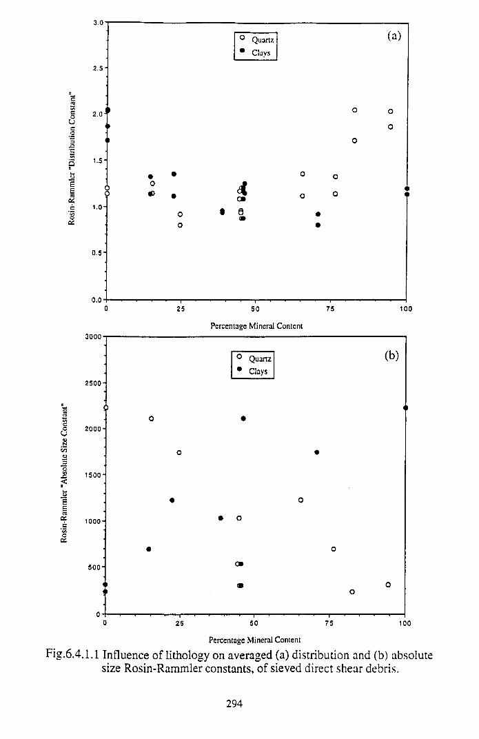
Rosin

-Ram

mler

"Di

strib

ution

Con

stant

1

3.0

2 .5 -

0 Q u a r tz

* Clays

(a)

1 .5 -

O

O

OO

$1.0 -

o«

o0

4cm• e

o o

0 O

0 .5 -

0.0-4— i— .— I— i— i— i— ------1------ -— I— .— i— i— ----- 1— .................... ...................0 25 5 0 75 100

Percentage Mineral Content

Percentage Mineral Content

Fig.6.4.1.1 Influence of lithology on averaged (a) distribution and (b) absolute size Rosin-Rammler constants, of sieved direct shear debris.

294

«•

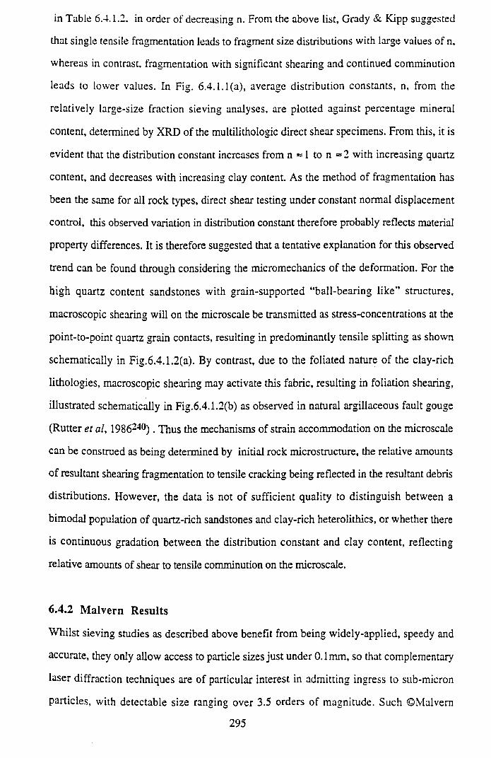
in Table 6.4.1.2, in order of decreasing n. From the above list, Grady & Kipp suggested

that single tensile fragmentation leads to fragment size distributions with large values of n,

whereas in contrast, fragmentation with significant shearing and continued comminution

leads to lower values. In Fig. 6.4.1.1(a), average distribution constants, n, from the

relatively large-size fraction sieving analyses, are plotted against percentage mineral

content, determined by XRD of the multilithologic direct shear specimens. From this, it is

evident that the distribution constant increases from n = 1 to n ® 2 with increasing quartz

content, and decreases with increasing clay content. As the method of fragmentation has

been the same for all rock types, direct shear testing under constant normal displacement

control, this observed variation in distribution constant therefore probably reflects material

property differences. It is therefore suggested that a tentative explanation for this observed

trend can be found through considering the micromechanics of the deformation. For the

high quartz content sandstones with grain-supported “ball-bearing like” structures,

macroscopic shearing will on the microscale be transmitted as stress-concentrations at the

point-to-point quartz grain contacts, resulting in predominantly tensile splitting as shown

schematically in Fig.6.4.1.2(a). By contrast, due to the foliated nature of the clay-rich

lithologies, macroscopic shearing may activate this fabric, resulting in foliation shearing,

illustrated schematically in Fig.6.4.1.2(b) as observed in natural argillaceous fault gouge

(Rutter et al, 1986240) . Thus the mechanisms of strain accommodation on the microscale

can be construed as being determined by initial rock microstructure, the relative amounts

of resultant shearing fragmentation to tensile cracking being reflected in the resultant debris

distributions. However, the data is not of sufficient quality to distinguish between a

bimodal population of quartz-rich sandstones and clay-rich heterolithics, or whether there

is continuous gradation between the distribution constant and clay content, reflecting

relative amounts of shear to tensile comminution on the microscale.

6.4.2 M alvern R esults

Whilst sieving studies as described above benefit from being widely-applied, speedy and

accurate, they only allow access to particle sizes just under 0.1mm, so that complementary

laser diffraction techniques are of particular interest in admitting ingress to sub-micron

particles, with detectable size ranging over 3.5 orders of magnitude. Such ©Malvern

295

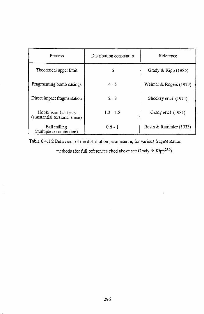
Process Distribution constant, n Reference

Theoretical upper limit 6 Grady & Kipp (1985)

Fragmenting bomb casings 4 - 5 Weimar & Rogers (1979)

Direct impact fragmentation 2 - 3 Shockeyera/ (1974)

Hopkinson bar tests (sunstantial torsional shear)

1.2 - 1.8 Grady etal (1981)

Ball milling (multiple comminution)

0 . 6 - 1 Rosin & Rammier (1933)

Table 6.4.1.2 Behaviour of the distribution parameter, n, for various fragmentation

methods (for full references cited above see Grady & Kipp239).

296

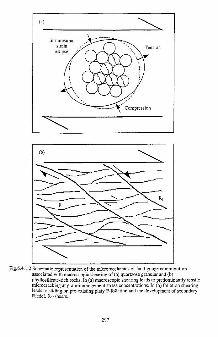
Fig.6.4.1.2 Schematic representation of the micromechanics of fault gouge comminution associated with macroscopic shearing of (a) quartzose granular and (b) phyllosilicate-rich rocks. In (a) macroscopic shearing leads to predominantly tensile microcracking at grain-impingement stress concentrations. In (b) foliation shearing leads to sliding on pre-existing platy P-foliation and the development of secondary Riedel, R [-shears.

297

Mastersizer studies utilised the <500micron-sized fraction detailed in Table 6.4.1,

suspended in distilled water as a supporting medium. The optical model employed by the

Mastersizer to compute volume distributions was customised by entering the optical

constants of the sample material and supporting medium, all direct shear powder samples

being treated as quartz, with a refractive index of 1.54. Also, for specific surface area (per

g of sample) calculations, all sample materials were assigned the specific gravity of quartz

= 2.65. Thus despite the polyminerallic nature of the direct shear specimens, with clay

contents ranging up to 100% (#9) operating restrictions forced the Mastersizer to regard all

experimental fault gouge powders as volume distributions of quartz spheres. Independent

powder samples from each direct shear specimen (BOT and TOP combined) were analysed

using the 300mm- and 45mm-range lenses, giving particle sizes extending from 600 to

1.2microns and 80 to 0.1 microns respectively. The analysis mode was set to model

independent, in which no assumption is made about the form of the result with regard to its

distribution.

Resultant cumulative weight oversize (%) versus particle size data was analysed using the

log-normal and Rosin-Rammler laws, and represented graphically as given in Fig.6.4.2.1

(red sandstones), Fig.6.4.2.2 (fissile mudstones), Fig.6.4.2.3 (carbonaceous siltstones)

and Fig.6.4.2.4 (heterolithics) using the methods outlined in section 6.2.4. This

Mastersizer data is complemented by superimposition of the sieving data detailed in section

6.4.1, for the purposes of comparison. With the exception of the fissile mudstone results,

good correlation is shown between the 300mm range lens data and sieving results.

Geometric means and standard deviations for the log-normal curves are given in Table

6.4.2.1, as well as distribution and absolute size constants characterising the Rosin-

Rammler plots. Due to the sigmoidal nature of some of these power-law distributions

(especially the fissile mudstones) straight line logarithmic regression fits were calculated for

the central portion of each curve, the particle size range of these fits also being given in

Table 6.4.2.1. The distribution constants, n, were converted to inferred fractal dimensions,

D, using the linear relation, D = 3 - n (Eqn.6.2.5.4).

298

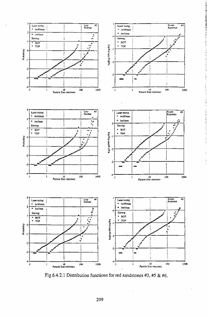
Prob

abili

ty

Prob

abili

ty

Prob

abili

tyLaser st/.ing:

■ t‘*300mm

Log- »3 } Normal

• f=a5mm j i * Sieving: j ••

• BOT j j• TOP !

1 .* '

1 / | . /\ y* ? y•

•»i

«1

.1 I tO 100 1000Particle Size (microns)

Laser sizing: ' Rosin- «1Rammlcr

* fa300mm :" i*a5mm +

Sieving: • i • X "

• b o t i / ; y• t o p i / ! y

J? *

•

1 J? y

/ f /M

mm

j

.1 t 10 100 1000Particle Size (microns)

Lasersizing: * fa 300mm

■ f»i5mm 1

Rosin- »6 Rammlcr

... J L -Sieving:

• BOT

• TOP

! jj j r

• n • -* * ■

• /

jT i \ • / 1 / b

y 1a

■

? r \ / I

-■ I

- j

i.1 I 10 100 1000

Panicle Size (microns)

Fig.6.4.2.1 Distribution functions for red sandstones #3, #5 & #6.

299

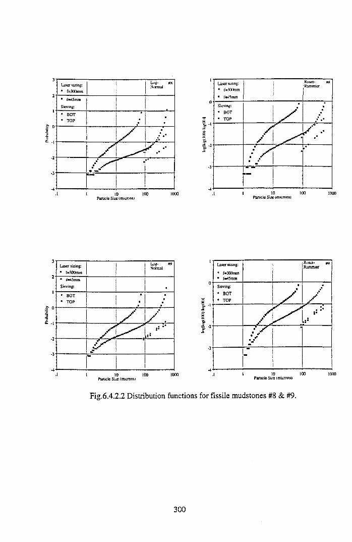
Prob

abili

ty

Prob

abili

ty

Laser sizing: * f=300mm

| i Log- «X ! Normal

• l'»45mm

Sieving: --------------- 1—• BOT• TOP

■

•«« m

■n* •*

« •

a r •* • •

im m

• • 1

.1 l 10 100 1000Panicle Size (microns»

Laser sizing:

■ I'aWKhnm

• M 5 m m

Rosin- «8 Rammicr

Sieving:

• BOT

* TO P

i k.

•

:

«■

■■■* •

/ f ^

/ !

_ j f •a •

•

m j/T

• /• «

m•

. I ” |f

i

.1 l 10 100 1000Panicle Size t microns)

Fig.6.4.2.2 Distribution functions for fissile mudstones #8 & #9.

300

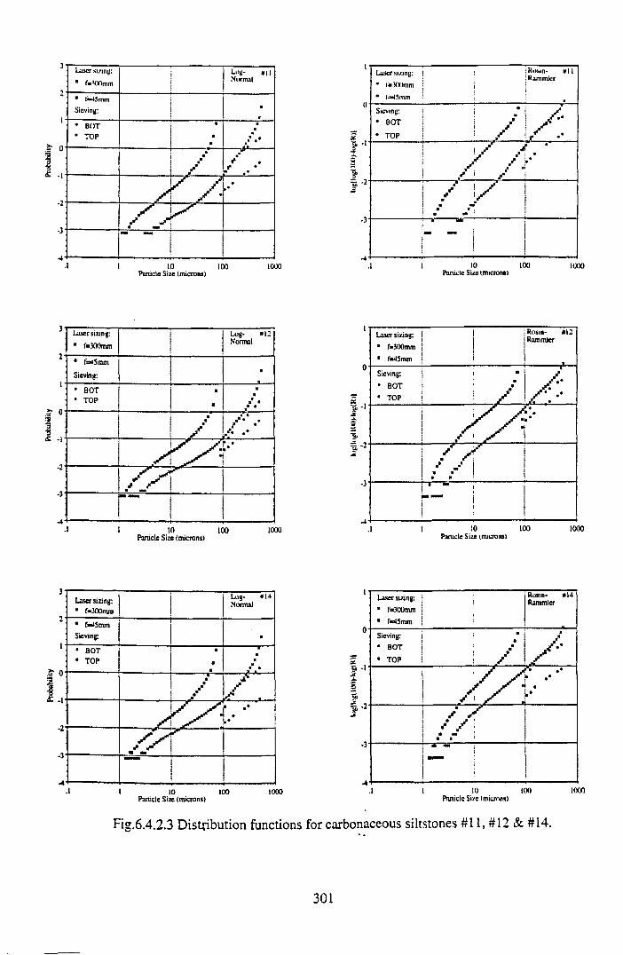
Prob

abili

ty

Prob

abili

ty

Prob

abili

ty

Laser sizing:

■ f»3(X)mmLog- # u Normal

■ t'*45mm

Sieving:ii a

*• BOT• TOP

■

1I ■

a

•

1 / / • / # •

L r *j / f / •

»•*

s j -a mmmam

.1 i 10 100 1000Particle Size (microns)

Laser sizing: i ¡Rosin- #11i RammJcr

* f»300mm | j |

• I'saaSmm B

Sieving:• BOT

• TOP

•••

//

A . / '

•»*

/ " [ / a aa"

.1 l 10 100 1000Parucle Size (.microns)

a-i

f '2

Laser sizing: | j

* f=300mm \ j

■ f*45mm |

Rosin- #14 RammJer

Sieving: i *• BOT |

• TOP 1 ! jA

/ / / • • -

/ / y/ S

/ /• m

m atb mm

i

I 10 100Particle Si/e fmiemns)

1000

Fig.6.4.2.3 Distribution functions for carbonaceous siltstones #11, #12 & #14.

301

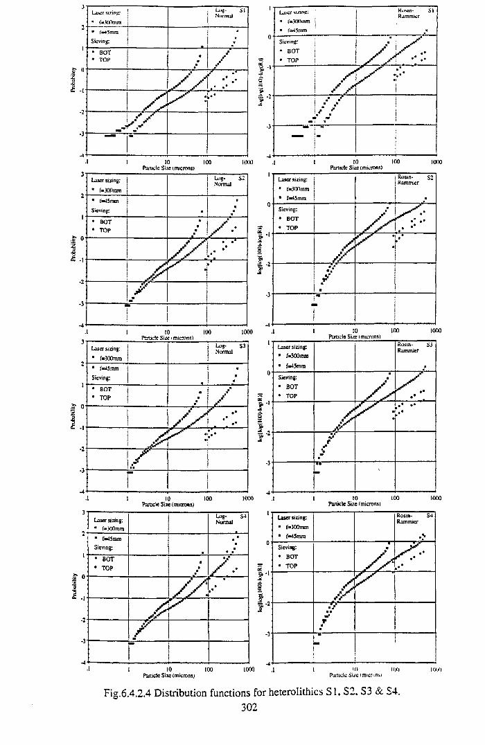
Prob

abili

ty

Prob

abili

ty

Prob

abili

ty

Prob

abili

ty

Laser siring: !i

■ fsJOOmm |

Log- SI Normal

■ f*45mm

Sieving:

• BOT• TOP

••■• /

... . ! X ?

• I I 10 100 1000Particle Sire (microns)

Laser string:

* f»300mm

Log- S2 Normal

• l'»45mm

Sieving; ■

■«

■

• BOT• TOP

••

••j r • jt■ •

. •* •

t . *

| j f4»

i X ! .1 m

a1 1 | !

.1 1 10 100 1000

leaser M/ing:■ i'a300mm i■ f»45mm

Knsin- SI Rammlcr

Sieving:

• BOT

• TOP ! r/K:1 /

X * / / |

» <rm »

1 / /• * m «m i m

ij

|I

.1 1 10 100 1000 Panicle Size (microns)

Fig.6.4.2.4 Distribution functions for heterolithics SI, S2, S3 & S4.302

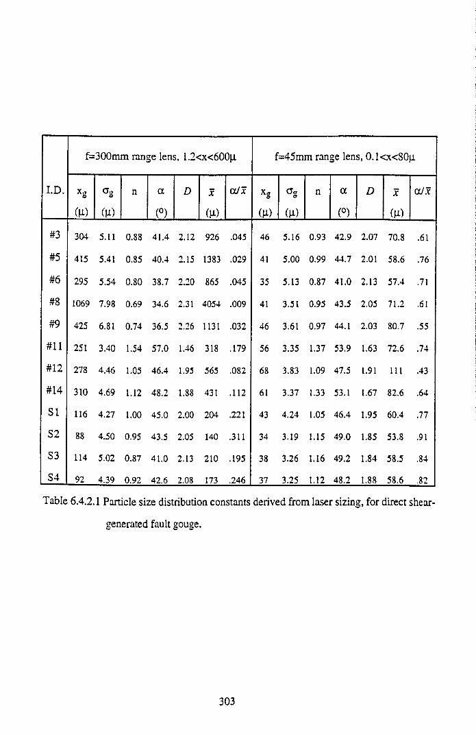
I.D.

f=300mm range lens, 1.2<x<600|i f=45mm range lens, 0.1<x<80n

XcT©

(It)

a ,te

(li)

n a

(°)

D X

(H)

a Jx XlTo

(u)

daO

(M-)

n a

(°)

D X

(n)

a/x

#3 304 5.11 0.88 41.4 2.12 926 .045 46 5.16 0.93 42.9 2.07 70.8 .61

#5 415 5.41 0.85 40.4 2.15 1383 .029 41 5.00 0.99 44.7 2.01 58.6 .76

#6 295 5.54 0.80 38.7 2.20 865 .045 35 5.13 0.87 41.0 2.13 57.4 .71

#8 1069 7.98 0.69 34.6 2.31 4054 .009 41 3.51 0.95 43.5 2.05 71.2 .61

#9 425 6.81 0.74 36.5 2.26 1131 .032 46 3.61 0.97 44.1 2.03 80.7 .55

#11 251 3.40 1.54 57.0 1.46 318 .179 56 3.35 1.37 53.9 1.63 72.6 .74

#12 278 4.46 1.05 46.4 1.95 565 .082 68 3.83 1.09 47.5 1.91 111 .43

#14 310 4.69 1.12 48.2 1.88 431 .112 61 3.37 1.33 53.1 1.67 82.6 .64

SI 116 4.27 1.00 45.0 2.00 204 .221 43 4.24 1.05 46.4 1.95 60.4 .77

S2 88 4.50 0.95 43.5 2.05 140 .311 34 3.19 1.15 49.0 1.85 53.8 .91

S3 114 5.02 0.87 41.0 2.13 210 .195 38 3.26 1.16 49.2 1.84 58.5 .84

S4 92 4.39 0.92 42.6 2.08 173 .246 37 3.25 1.12 48.2 1.88 58.6 .82

Table 6.4.2.1 Particle size distribution constants derived from laser sizing, for direct shear­

generated fault gouge.

303

With the possible exception of specimen SI, visual observation of the strongly sigmoidal

expression of the log-normal probability plots, suggests that this function does not have

wide application for the direct shear gouge distributions (it should be noted however that

both the natural and experimental fault gouge distributions described by Engelder (1974)6

as being log-normal over much more restricted particle size ranges determined from

sieving, also showed similar sigmoidal profiles). In general, the deviation of each graph

from the straight line indicates a corresponding deviation of the particle size distribution

from normality. The slope of the curve is a measure of particle sorting, sorting deteriorating

with decreasing slope. Using this method, Engelder found the sorting of experimental

quartz fault gouge deformed under triaxial compression, to decrease both with increasing

confining pressure and with increasing shear displacement. A general trend is apparent

amongst the quartz-rich/clay-poor sample plots generated by the 300mm-range lens (#3,

#5, #6, #11, #12, #14, S I) for initially steep slopes down to particle sizes of around

lOOmicrons, parallel to the sieve data, followed by shallower slopes which remain linear

down to the lowest limits of the measuring range. Such convex downwards curves

represent a change in sorting at about the 0.1mm particle size, which may reflect relatively

well-sorted initial grains which have not been fragmented, contained within a fine-grained

matrix of comminuted debris representing steady-state size reduction down to the limits of

particle size resolution. In contrast, the clay-rich/quartz-poor samples (#8, #9, S2, S3, S4)

exhibit strongly sigmoidal curves, which reflect initial decrease in sorting, followed by an

increase in sorting down to around lmicron, representing the lower limit of particle size.

The fact that both the 300mm- and 45mm-range lens data converge at this lower limit of

around lmicron, strongly suggests that the argillaceous samples achieve a minimum

comminution limit. This observation indicates that the comminution efficiency of the clay-

rich specimens is reduced at small particle size, compared to that of the quartz-rich

specimens, which may reflect the nature of the inter-particle stress concentrations for the

different mineral phases. This could well be due to the relative shape factors of the clay and

quartz fractions, however it is also possible that plastic deformation, as opposed to

fracturing and increase in new surface area, may be occurring in the clay phase.

Interestingly, Mackenzie & Milne (1953)241 showed that the X-ray diffraction pattern of

muscovite becomes more diffuse as industrial grinding proceeds until, after Shours, no

304

sharp pattern remains. After further grinding the pattern reappears but has a different form

to the original, suggesting the possibility of recrystallisation.

The power-law (fractal) distribution curves for the direct shear debris samples, show fairly

robust approximations to linearity for the quartz-rich specimens, over the entire

measurement range, however, as observed for the log-normal plots, specimens with clay

contents >50% (#8, #9, S2, S3, S4) show sigmoidal trends with both the laser-sized

distributions converging at around 1 micron. For the purposes of comparison, straight-line

logarithmic regression fits were constructed for the linear mid-sections of all 12 direct shear

power-law distributions, in order to determine fractal dimensions for the fault gouge

samples. Whilst scale-invariance is inherent in the definition of a fractal or fractional

dimension, “natural” as opposed to “mathematical” fractals do possess finite upper and

lower fractal limits above and below which this scale invariance breaks down. The direct

shear fractal dimension magnitudes are given in Table 6.4.2.1. From this, it is evident that

the magnitude of D lies in the range 1.5<D <2.4 and \.1<D <2.2 for f=300mm and

f=45mm respectively, both limits lying within the range of published magnitudes for a

diverse range of fractal fragment-size distributions (see for example Table 6.2.5.1).

6.4.3 Frictional Strength Correlations and Surface Energy Considerations

For the direct shear experimental programme, in which shearing was conducted under

constant normal displacement conditions conducive to maximum gouge production (post­

maximum frictional slip occurring wholly upon a substrate of comminuted shear debris) it

is obviously of interest to investigate any relations between the nature of the fragmented

wear products, and the frictional strength of the sliding interfaces. Whilst no correlation

was found between either of the parameters describing the log-normal distribution (xg and

a g in Table 6.4.2.1) and the frictional strength parameters (|i*max in Table 3.5.1.1, |is and

S0 for constant and variable contact areas in Table 3.5.3.1) presumably due to the poor

applicability of this distribution function, correlation was indeed evident between fractal

dimension, D, as listed in Table 6.4.2.1, and p.s. Whilst correlation between |i s, and D

-values from the 300mm-range lens was evident, better correlation was shown with the

45mm data, illustrated in Fig.6.4.3.1. From this plot it is evident that the magnitude of the

305

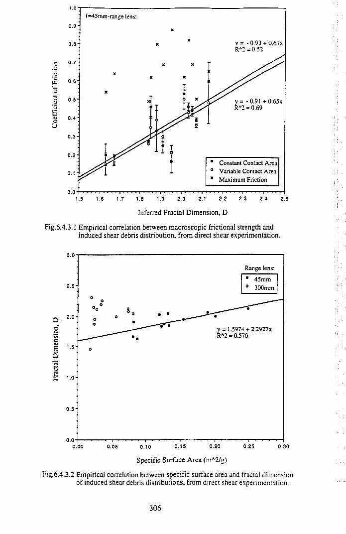
Inferred Fractal Dimension, D

Fig.6.4.3.1 Empirical correlation between macroscopic frictional strength and induced shear debris distribution, from direct shear experimentation.

Fig.6.4.3.2 Empirical correlation between specific surface area and fractal dimension of induced shear debris distributions, from direct shear experimentation.

306

maximum friction is independent of the fractal dimension of the induced gouge, which is to

be expected if ¡i*max represents maximum interlocking of asperities, prior to pervasive

shearing of roughness and frictional sliding upon a comminuted substrate.

As higher values of D indicate higher numbers of small fragments relative to larger

fragments than in populations with lower fractal dimensions, and as surface area varies

inversely with particle size (see Eqn.6.4.1.2), intuitively it follows that higher D indicates

greater surface area. This relation is borne out between the empirically determined

correlation between specific surface area, Sw, calculated for the 45mm-range lens data

using Eqn.6.4.1.2, and the fractal dimension, D, as given in Fig.6.4.3.2. No correlation is

evident between D and Sw as determined from the 300mm-range lens data, although it is

pointed out that maximum surface area determination is generated from the smallest particle

size measurements, as shown by Table 6.4.3.1, which lists volume-surface mean particle

sizes and weight specific surfaces for the two laser measurement ranges. The coefficient of

sliding friction, p s, also correlates with the model independent, volume-surface mean

particle size determinations of specific surface area, as shown in Fig.6.4.3.3.

Olgaard & Brace (1983)242 studied quartz fault gouge from two mining-induced seismic

shear fractures, in order to determine that portion of the total strain energy released during

an earthquake that is allocated to the creation of new surface area (fault gouge). They noted

that the three principal sinks for the strain energy released during faulting are heat, seismic

waves and microstructural defects formed during crushing (as new surface area is the

principal defect produced at shallow crustal levels, this "defect" energy is mostly surface

energy). Olgaard & Brace estimated the surface area energy, Wa , that is the amount of

energy consumed in creating new surfaces, using the relation:

W a = Sw-P-Y .......... Eqn.6.4.3.1

Wa : energy density, the energy per unit volume (JmA-3)

S\y: specific surface area per gram of powder (mA2kgA-1)

307

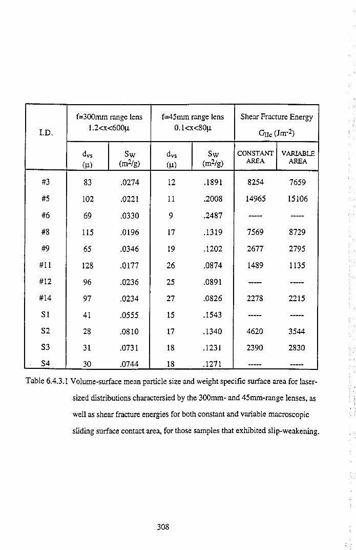
I.D.

f=300mm range lens 1.2<x<600|i

f=45mm range lens 0.1<x<80(i

Shear Fracture Energy

G iicdm -2)

dVs Sw dVs Sw CONSTANT VARIABLE(H) (m2/g) (it) (m2/g) AREA AREA

#3 83 .0274 12 .1891 8254 7659

#5 102 .0221 11 .2008 14965 15106

#6 69 .0330 9 .2487 —

#8 115 .0196 17 .1319 7569 8729

#9 65 .0346 19 .1202 2677 2795

#11 128 .0177 26 .0874 1489 1135

#12 96 .0236 25 .0891

#14 97 .0234 27 .0826 2278 2215

SI 41 .0555 15 .1543

S2 28 .0810 17 .1340 4620 3544

S3 31 .0731 18 .1231 2390 2830

S4 30 .0744 18 .1271

Table 6.4.3.1 Volume-surface mean particle size and weight specific surface area for laser­

sized distributions charactersied by the 300mm- and 45mm-range lenses, as

well as shear fracture energies for both constant and variable macroscopic

sliding surface contact area, for those samples that exhibited slip-weakening.

308

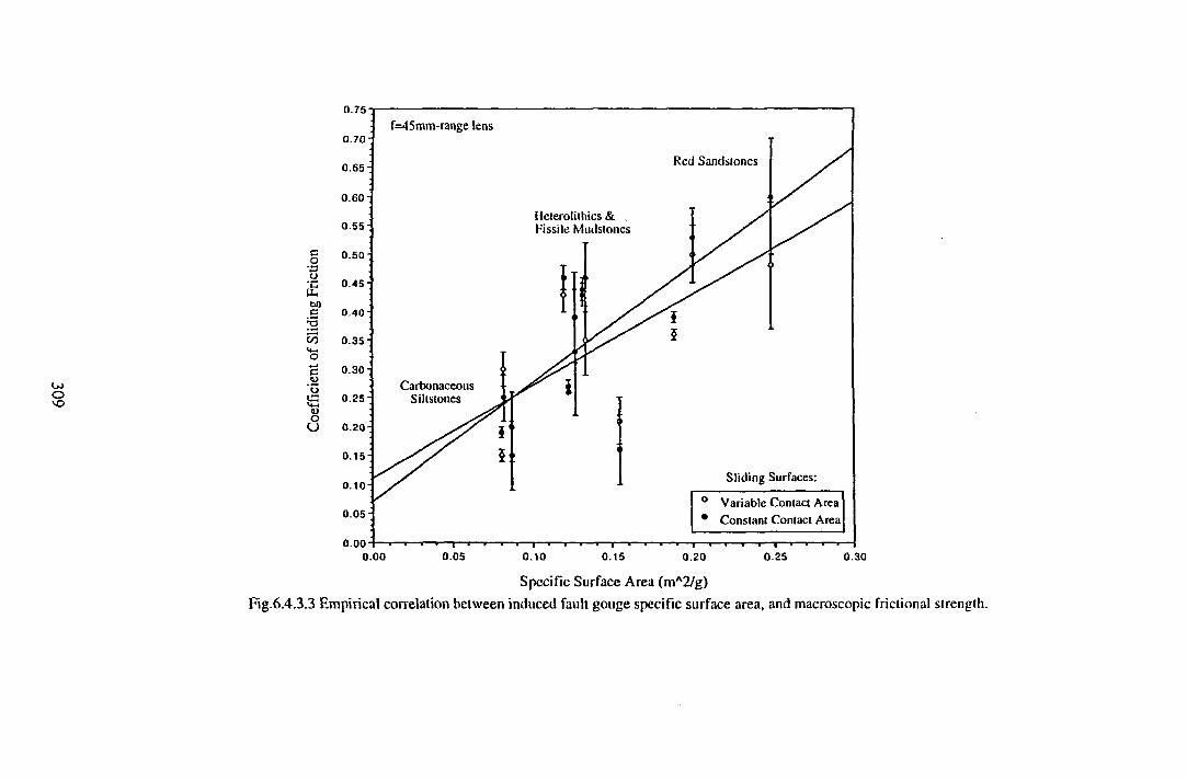
Specific Surface Area (mA2/g)Fig.6.4.3.3 Empirical correlation between induced fault gouge specific surface area, and macroscopic frictional strength.

p: density of the single mineral phase (kgmA-3)

y. specific surface energy of single crystal determined in tension (JmA-2)

For quartz fault gouge with S\y=2.0m-/g, 7^0.7J/m2 and p=2.65 x 103kg/m3, Olgaard &

Brace calculated WA=3.7 x 106J/m3. They then compared this value for with the total

energy released during an earthquake, Ex:

Ea/Et = (Wa .A.u)/Et .......... Eqn.6.4.3.2

A: area of fault plane

u: width of fault gouge zone

From Brune (1968)243, Ex = A.d.cx where d is the average fault displacement, and a is

the average stress on the fault. Thus for typical mine values of A, u, d and a , they

calculated that Ea/Et = 1 - 9%, that is the surface energy is of the same order of magnitude

as the seismic energy, with heat thus representing the principal energy sink. This is in

agreement with Engelder et al (1975)244 for experimental sliding under triaxial

compression of pre-cut Tennessee sandstone on an artificial layer of quartz fault gouge,

who likewise found the increase in surface energy to be a negligible fraction of the total

work done (=0.1%).

From Eqn.6.4.3.1, it is evident that the energy density varies directly with the specific

surface area, suggesting that, possibly, the positive linear correlation of frictional strength

with both S\y and D, may reflect an increase in frictional resistance associated with an

increase in the energy required to create new surface area. However, Eqn.6.4.3.1 also

highlights the fact that a reasonable estimate of WA depends heavily upon the accuracy of

the measurement o f S\y- Olgaard & Brace242 used a combination of scanning and

transmission electron microscopy, X-ray sedimentation and gas adsorption to measure Sw,

and to study particle size and shape in the submicron-size region. Unfortunately, however,

the laser-sizing method, whilst able to measure over a wide particle-size range, assumes a

310

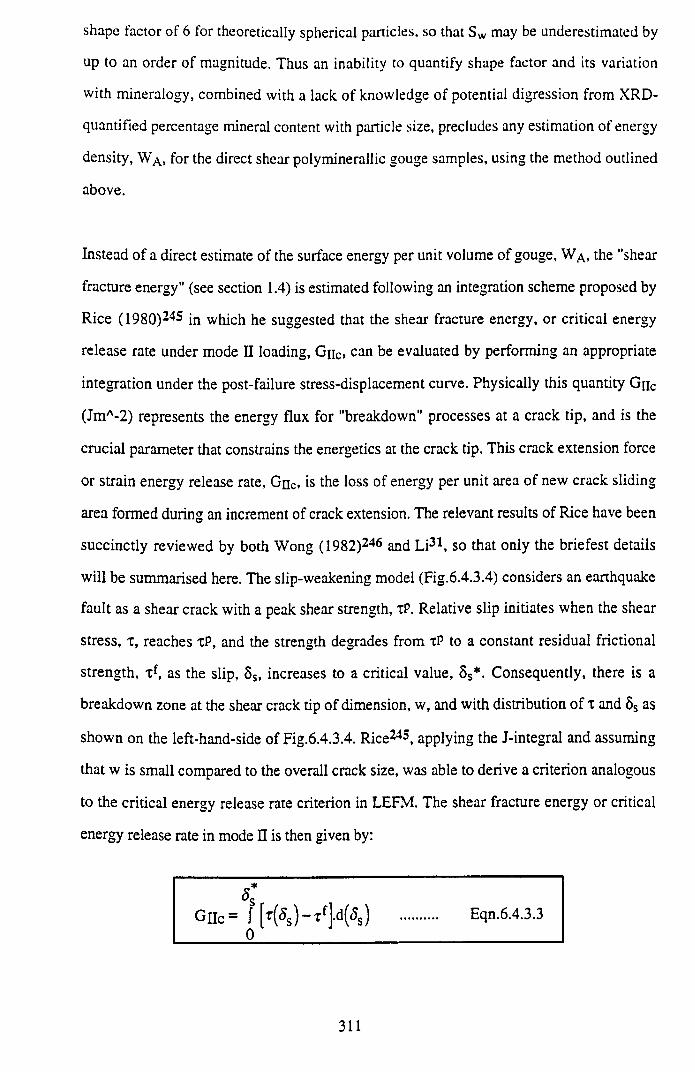
shape factor of 6 for theoretically spherical panicles, so that Sw may be underestimated by

up to an order of magnitude. Thus an inability to quantify shape factor and its variation

with mineralogy, combined with a lack of knowledge of potential digression from XRD-

quantified percentage mineral content with panicle size, precludes any estimation of energy

density, W ^, for the direct shear polyminerallic gouge samples, using the method outlined

above.

Instead of a direct estimate of the surface energy per unit volume of gouge, Wa , the "shear

fracture energy" (see section 1.4) is estimated following an integration scheme proposed by

Rice (1980)245 in which he suggested that the shear fracture energy, or critical energy

release rate under mode II loading, Giic. can be evaluated by performing an appropriate

integration under the post-failure stress-displacement curve. Physically this quantity Gnc

(JmA-2) represents the energy flux for "breakdown" processes at a crack tip, and is the

crucial parameter that constrains the energetics at the crack tip. This crack extension force

or strain energy release rate, Gnc. is the loss of energy per unit area of new crack sliding

area formed during an increment of crack extension. The relevant results of Rice have been

succinctly reviewed by both Wong (1982)246 and Li31, so that only the briefest details

will be summarised here. The slip-weakening model (Fig.6.4.3.4) considers an earthquake

fault as a shear crack with a peak shear strength, tP. Relative slip initiates when the shear

stress, x, reaches xP, and the strength degrades from xP to a constant residual frictional

strength, xf, as the slip, 8S, increases to a critical value, 8S*. Consequently, there is a

breakdown zone at the shear crack tip of dimension, w, and with distribution of X and 8S as

shown on the left-hand-side of Fig.6.4.3.4. Rice245, applying the J-integral and assuming

that w is small compared to the overall crack size, was able to derive a criterion analogous

to the critical energy release rate criterion in LEFM. The shear fracture energy or critical

energy release rate in mode II is then given by:

0Eqn.6.4.3.3

311

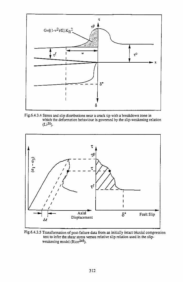
Fig.6.4.3.4 Stress and slip distributions near a crack tip with a breakdown zone inwhich the deformation behaviour is governed by the slip-weakening relation (Li31).

Fig.6.4.3.5 Transformation of post-failure data from an initially intact triaxial compression test to infer the shear stress versus relative slip relation used in the slip­weakening model (Rice245).

312

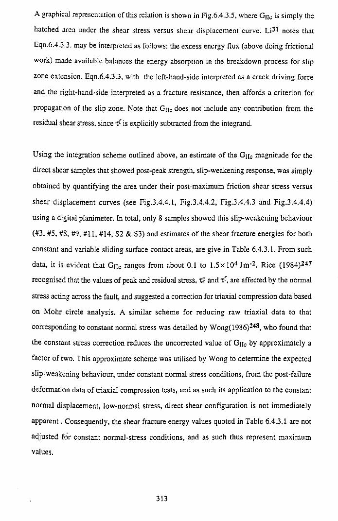
A graphical representation of this relation is shown in Fig.6.4.3.5, where G jic is simply the

hatched area under the shear stress versus shear displacement curve. Li21 notes that

Eqn.6.4.3.3. may be interpreted as follows: the excess energy flux (above doing frictional

work) made available balances the energy absorption in the breakdown process for slip

zone extension. Eqn.6.4.3.3, with the left-hand-side interpreted as a crack driving force

and the right-hand-side interpreted as a fracture resistance, then affords a criterion for

propagation of the slip zone. Note that Gnc does not include any contribution from the

residual shear stress, since xf is explicitly subtracted from the integrand.

Using the integration scheme outlined above, an estimate of the Gnc magnitude for the

direct shear samples that showed post-peak strength, slip-weakening response, was simply

obtained by quantifying the area under their post-maximum friction shear stress versus

shear displacement curves (see Fig.3.4.4.1, Fig.3.4.4.2, Fig.3.4.4.3 and Fig.3.4.4.4)

using a digital planimeter. In total, only 8 samples showed this slip-weakening behaviour

(#3, #5, #8, #9, #11, #14, S2 & S3) and estimates of the shear fracture energies for both

constant and variable sliding surface contact areas, are give in Table 6.4.3.1. From such

data, it is evident that Giic ranges from about 0.1 to 1 .5 x l0 4 Jm*2. Rice (1984)247

recognised that the values of peak and residual stress, tP and xf, are affected by the normal

stress acting across the fault, and suggested a correction for triaxial compression data based

on M ohr circle analysis. A similar scheme for reducing raw triaxial data to that

corresponding to constant normal stress was detailed by Wong(1986)248, who found that

the constant stress correction reduces the uncorrected value of Gnc by approximately a

factor of two. This approximate scheme was utilised by Wong to determine the expected

slip-weakening behaviour, under constant normal stress conditions, from the post-failure

deformation data of triaxial compression tests, and as such its application to the constant

normal displacement, low-normal stress, direct shear configuration is not immediately

apparent. Consequently, the shear fracture energy values quoted in Table 6.4.3.1 are not

adjusted for constant normal-stress conditions, and as such thus represent maximum

values.

313

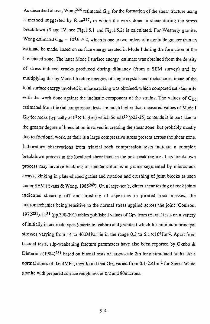
As described above, Wong246 estimated Guc for the formation of the shear fracture using

a method suggested by Rice247, in which the work done in shear during the stress

breakdown (Stage IV, see Fig. 1.5.1 and Fig. 1.5.2) is calculated. For Westerly granite,

Wong estimated Gnc ~ 104JmA-2, which is one to two orders of magnitude greater than an

estimate he made, based on surface energy created in Mode I during the formation of the

brecciated zone. The latter Mode I surface energy estimate was obtained from the density

of stress-induced cracks produced during dilatancy (from a SEM survey) and by

multiplying this by Mode I fracture energies of single crystals and rocks, an estimate of the

total surface energy involved in microcracking was obtained, which compared satisfactorily

with the work done against the inelastic component of the strains. The values of Gnc

estimated from triaxial compression tests are much higher than measured values of Mode I

Gic for rocks (typically >102x higher) which Scholz16 (p23-25) contends is in part due to

the greater degree of brecciation involved in creating the shear zone, but probably mostly

due to frictional work, as their is a large compressive stress present across the shear zone.

Laboratory observations from triaxial rock compression tests indicate a complex

breakdown process in the localised shear band in the post-peak regime. This breakdown

process may involve buckling of slender columns in grains segmented by microcrack

arrays, kinking in plate-shaped grains and rotation and crushing of joint blocks as seen

under SEM (Evans & Wong, 1985249). On a large-scale, direct shear testing of rock joints

indicates shearing off and crushing of asperities in jo in ted rock masses, the

micromechanics being sensitive to the normal stress applied across the joint (Coulson,

1972251). Li31 (pp.390-391) tables published values of Gnc from triaxial tests on a variety

of initially intact rock types (quartzite, gabbro and granites) which for minimum principal

stresses varying from 14 to 400MPa, lie in the range 0.3 to 5.1 X 104Jm*2. Apart from

triaxial tests, slip-weakening fracture parameters have also been reported by Okubo &

Dieterich (1984)251 based on biaxial tests of large-scale 2m long simulated faults. At a

normal stress of 0.6-4MPa, they found that Gnc varied from 0. l-2 .4Jnr2 for Sierra White

granite with prepared surface roughness of 0.2 and 80microns.

314

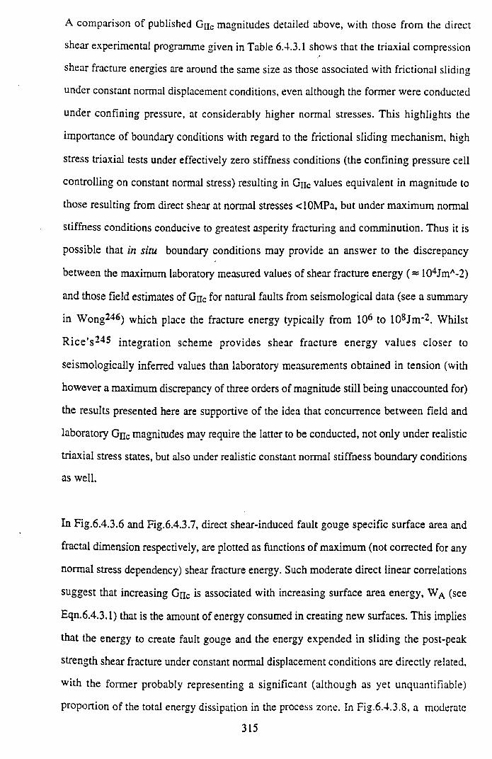
A comparison of published Guc magnitudes detailed above, with those from the direct

shear experimental programme given in Table 6.4.3.1 shows that the triaxial compression

shear fracture energies are around the same size as those associated with frictional sliding

under constant normal displacement conditions, even although the former were conducted

under confining pressure, at considerably higher normal stresses. This highlights the

importance of boundary conditions with regard to the frictional sliding mechanism, high

stress triaxial tests under effectively zero stiffness conditions (the confining pressure cell

controlling on constant normal stress) resulting in Gnc values equivalent in magnitude to

those resulting from direct shear at normal stresses clOMPa, but under maximum normal

stiffness conditions conducive to greatest asperity fracturing and comminution. Thus it is

possible that in situ boundary conditions may provide an answer to the discrepancy

between the maximum laboratory measured values of shear fracture energy (= 104JmA-2)

and those field estimates of Gnc for natural faults from seismological data (see a summary

in Wong246) which place the fracture energy typically from 106 to 108Jm*2. Whilst

R ic e ’s 245 integration scheme provides shear fracture energy values closer to

seismologically inferred values than laboratory measurements obtained in tension (with

however a maximum discrepancy of three orders of magnitude still being unaccounted for)

the results presented here are supportive of the idea that concurrence between field and

laboratory Gnc magnitudes may require the latter to be conducted, not only under realistic

triaxial stress states, but also under realistic constant normal stiffness boundary conditions

as well.

In Fig.6.4.3.6 and Fig.6.4.3.7, direct shear-induced fault gouge specific surface area and

fractal dimension respectively, are plotted as functions of maximum (not corrected for any

normal stress dependency) shear fracture energy. Such moderate direct linear correlations

suggest that increasing Gnc is associated with increasing surface area energy, W ^ (see

Eqn.6.4.3.1) that is the amount of energy consumed in creating new surfaces. This implies

that the energy to create fault gouge and the energy expended in sliding the post-peak

strength shear fracture under constant normal displacement conditions are directly related,

with the former probably representing a significant (although as yet unquantifiable)

proportion of the total energy dissipation in the process zone. In Fig.6.4.3.8, a moderate

315

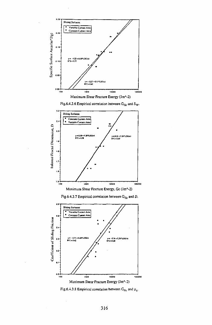
Infe

rred

Fra

ctal

Dim

ensi

on, D

Sp

ecifi

c Su

rfac

e A

rea

(mA2

/g)

Maximum Shear Fracture Energy (JmA-2)

Fig.6.4.3.6 Empirical correlation between G|lc and Sw.

Maximum Shear Fracture Energy, Gc (JmA-2)

Fig.6.4.3.7 Empirical cotTelation between Guc and D.

Fig.6.4.3.8 Empirical correlation between GIU; and (is.

316

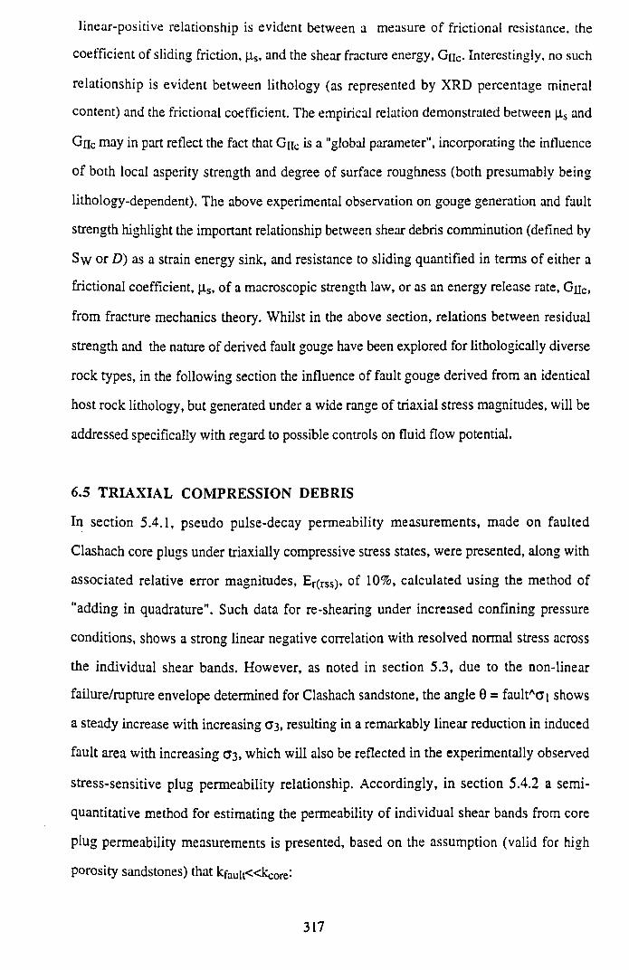
linear-positive relationship is evident between a measure of frictional resistance, the

coefficient of sliding friction, p.s, and the shear fracture energy, G[jc. Interestingly, no such

relationship is evident between lithology (as represented by XRD percentage mineral

content) and the frictional coefficient. The empirical relation demonstrated between |is and

Gnc may in part reflect the fact that Gnc is a "global parameter", incorporating the influence

of both local asperity strength and degree of surface roughness (both presumably being

lithology-dependent). The above experimental observation on gouge generation and fault

strength highlight the important relationship between shear debris comminution (defined by

Sw or D) as a strain energy sink, and resistance to sliding quantified in terms of either a

frictional coefficient, jis, of a macroscopic strength law, or as an energy release rate, Gnc,

from fracture mechanics theory. Whilst in the above section, relations between residual

strength and the nature of derived fault gouge have been explored for lithologically diverse

rock types, in the following section the influence of fault gouge derived from an identical

host rock lithology, but generated under a wide range of triaxial stress magnitudes, will be

addressed specifically with regard to possible controls on fluid flow potential.

6.5 TR IA X IA L CO M PRESSIO N DEBRIS

In section 5.4.1, pseudo pulse-decay permeability measurements, made on faulted

Clashach core plugs under triaxially compressive stress states, were presented, along with

associated relative error magnitudes, Er(rsS), of 10%, calculated using the method of

"adding in quadrature". Such data for re-shearing under increased confining pressure

conditions, shows a strong linear negative correlation with resolved normal stress across

the individual shear bands. However, as noted in section 5.3, due to the non-linear

failure/rupture envelope determined for Clashach sandstone, the angle 0 = faultAa i shows

a steady increase with increasing G3, resulting in a remarkably linear reduction in induced

fault area with increasing G 3 , which will also be reflected in the experimentally observed

stress-sensitive plug permeability relationship. Accordingly, in section 5.4.2 a semi-

quantitative method for estimating the permeability of individual shear bands from core

plug permeability measurements is presented, based on the assumption (valid for high

porosity sandstones) that kfauit« k c 0re:

317

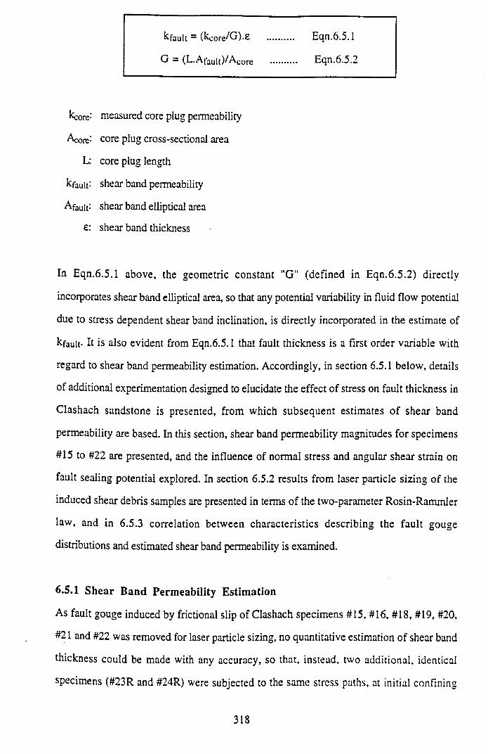
kfault — (kcore/G).£ ..... Eqn.6.5.1

G = (L.AfaUit)/Acore ..... Eqn.6.5.2

kcore: measured core plug permeability

Ac0re: core plug cross-sectional area

L: core plug length

kfault: shear band permeability

Afauit: shear band elliptical area

e: shear band thickness

In Eqn.6.5.1 above, the geometric constant "G" (defined in Eqn.6.5.2) directly

incorporates shear band elliptical area, so that any potential variability in fluid flow potential

due to stress dependent shear band inclination, is directly incorporated in the estimate of

kfault- It is also evident from Eqn.6.5.1 that fault thickness is a first order variable with

regard to shear band permeability estimation. Accordingly, in section 6.5.1 below, details

of additional experimentation designed to elucidate the effect of stress on fault thickness in

Clashach sandstone is presented, from which subsequent estimates of shear band

permeability are based. In this section, shear band permeability magnitudes for specimens

#15 to #22 are presented, and the influence of normal stress and angular shear strain on

fault sealing potential explored. In section 6.5.2 results from laser particle sizing of the

induced shear debris samples are presented in terms o f the two-parameter Rosin-Rammler

law, and in 6.5.3 correlation between characteristics describing the fault gouge

distributions and estimated shear band permeability is examined.

6.5.1 Shear Band Permeability Estimation

As fault gouge induced by frictional slip of Clashach specimens #15, #16, #18, #19, #20,

#21 and #22 was removed for laser particle sizing, no quantitative estimation of shear band

thickness could be made with any accuracy, so that, instead, two additional, identical

specimens (#23R and #24R) were subjected to the same stress paths, at initial confining

318

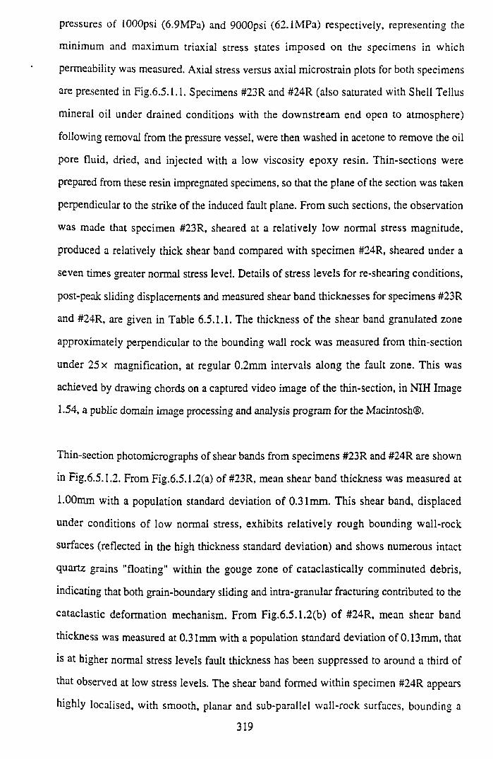
pressures ot lOOOpsi (6.9MPa) and 9000psi (62.1MPa) respectively, representing the

minimum and maximum triaxial stress states imposed on the specimens in which

permeability was measured. Axial stress versus axial microstrain plots for both specimens

are presented in Fig.6.5.1.1. Specimens #23R and #24R (also saturated with Shell Tellus

mineral oil under drained conditions with the downstream end open to atmosphere)

following removal from the pressure vessel, were then washed in acetone to remove the oil

pore fluid, dried, and injected with a low viscosity epoxy resin. Thin-sections were

prepared from these resin impregnated specimens, so that the plane of the section was taken

perpendicular to the strike of the induced fault plane. From such sections, the observation

was made that specimen #23R, sheared at a relatively low normal stress magnitude,

produced a relatively thick shear band compared with specimen #24R, sheared under a

seven times greater normal stress level. Details of stress levels for re-shearing conditions,

post-peak sliding displacements and measured shear band thicknesses for specimens #23R

and #24R, are given in Table 6.5.1.1. The thickness o f the shear band granulated zone

approximately perpendicular to the bounding wall rock was measured from thin-section

under 25 x magnification, at regular 0.2mm intervals along the fault zone. This was

achieved by drawing chords on a captured video image of the thin-section, in NIH Image

1.54, a public domain image processing and analysis program for the Macintosh®.

Thin-section photomicrographs of shear bands from specimens #23R and #24R are shown

in Fig.6.5.1.2. From Fig.6.5.1.2(a) of #23R, mean shear band thickness was measured at

1.00mm with a population standard deviation of 0.31mm. This shear band, displaced

under conditions of low normal stress, exhibits relatively rough bounding wall-rock

surfaces (reflected in the high thickness standard deviation) and shows numerous intact

quartz grains "floating" within the gouge zone of cataclastically comminuted debris,

indicating that both grain-boundary sliding and intra-granular fracturing contributed to the

cataclastic deformation mechanism. From Fig.6.5.1.2(b) o f #24R, mean shear band

thickness was measured at 0.31mm with a population standard deviation of 0.13mm, that

is at higher normal stress levels fault thickness has been suppressed to around a third of

that observed at low stress levels. The shear band formed within specimen #24R appears

highly localised, with smooth, planar and sub-parallel wall-rock surfaces, bounding a

319

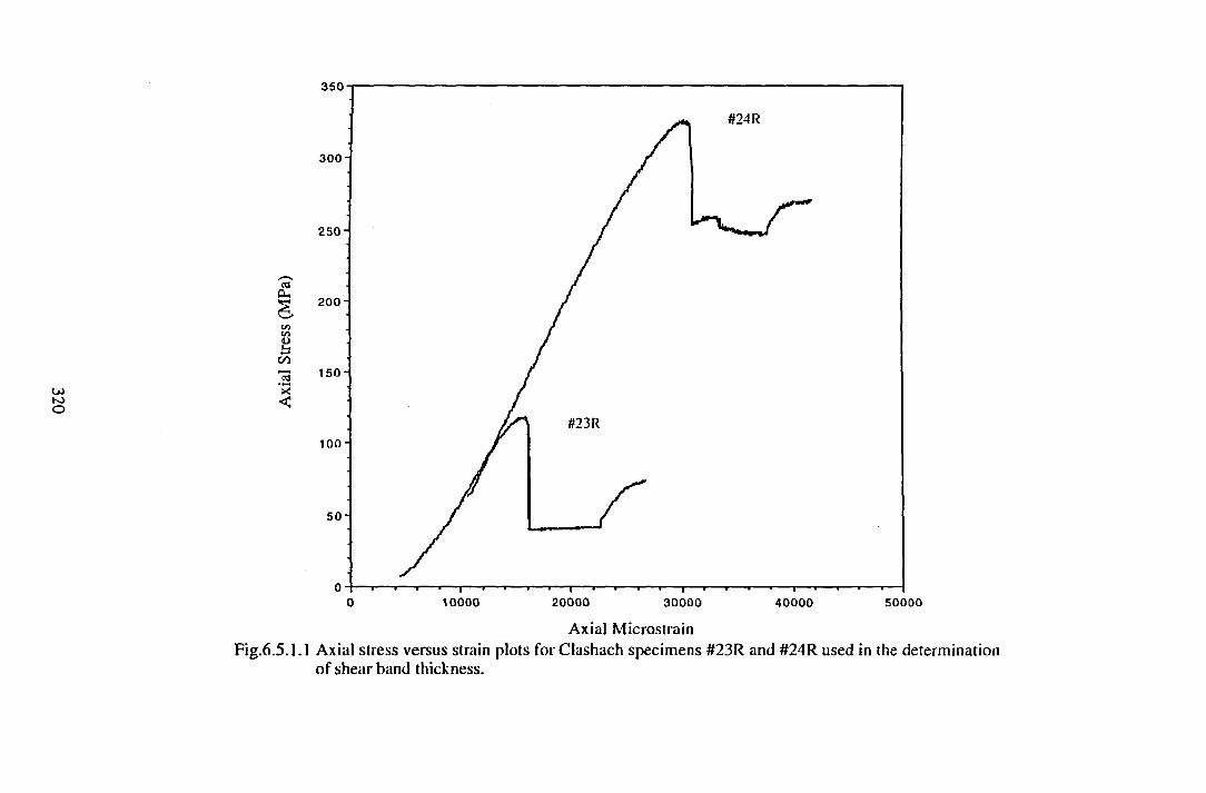
Axi

al S

tress

(M

Pa)

0 1 0 0 0 0 2 0 0 0 0 3 0 0 0 0 4 0 0 0 0 5 0 0 0 0

Axial MicrostrainFig.6.5.1.1 Axial stress versus strain plots for Clashach specimens #23R and #24R used in the determination

of shear band thickness.

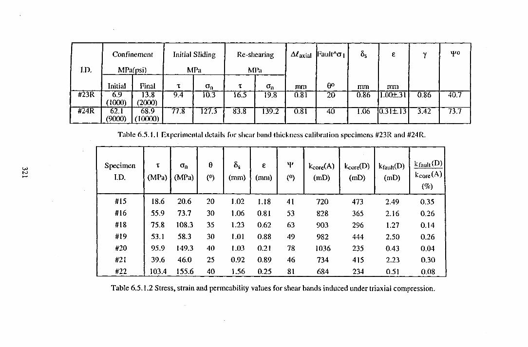
Confinement Initial Sliding Re-shearing Af axial FaultAa i 6s £ 7 ipo

ID. MPa(psi) MPa MPa

Initial Final X On X On mm 0° mm mm#23R 6.9

(1000)13.8

(2000)9.4 10.3 16.5 19.8 0.81 20 0.86 1.00+31 0.86 40.7

#24 R 62.1(9000)

68.9(10000)

77.8 127.3 83.8 139.2 0.81 40 1.06 0.31±. 13 3.42 73.7

Table 6 .5 .1. 1 Experimental details for shear band thickness calibration specimens #23R and #24R.

Specimen

I.D.

X

(MPa)o n

(MPa)

6

(°)

8s

(mm)

£

(mm)

T

(°)

kcore(A-)(mD)

kcore(D)

(mD)kfault(D)

(mD)

k fault (D)kcore(A)

(%)

#15 18.6 20.6 20 1.02 1.18 41 720 473 2.49 0.35#16 55.9 73.7 30 1.06 0.81 53 828 365 2.16 0.26#18 75.8 108.3 35 1.23 0.62 63 903 296 1.27 0.14#19 53.1 58.3 30 1.01 0.88 49 982 444 2.50 0.26#20 95.9 149.3 40 1.03 0.21 78 1036 235 0.43 0.04#21 39.6 46.0 25 0.92 0.89 46 734 415 2.23 0.30#22 103.4 155.6 40 1.56 0.25 81 684 234 0.51 0.08

Table 6.5.1.2 Stress, strain and permeability values for shear bands induced under triaxial compression.

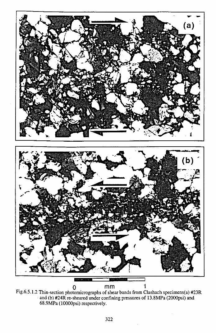
0 mm 1Fig.6.5.1.2 Thin-section photomicrographs of shear bands from Clashach specimens(a) #23R

• and (b) #24R re-sheared under confining pressures of 13.8MPa (2000psi) and 68.9MPa (lOOOOpsi) respectively.

322

gouge zone composed of highly comminuted grain-fragments in which intra-granular

cracking has exclusively dominated the cataclastic process. Such observations are

supported by those of Tullis & Yund (1992)252 on the effects of increasing confining

pressure (at temperatures <300°C) on the nature of faulting in feldspar (Bushveld

anorthosite) aggregates. Tullis & Yund noted that at lower pressures the gouge zone was

wider, which they attributed to its development from more irregular surfaces which break

off more material as they slide, whilst at higher pressures the faults were sharp and smooth

from the start, so that they could slide with less gouge development. Interestingly, a related

aspect recognised by Tullis & Yund was that a wider range of fragment sizes developed in

gouge formed at low pressures, compared with ubiquitously fine-grained fragment

development at high pressure.

Archard (1953)253 proposed a theory of wear (surface damage and erosion resulting from

frictional sliding) which, although quantitatively describing the main properties of the

process, is not specific about the mechanism by which wear particles are removed from the

surface (adhesive wear or abrasive wear) and hence finds general application. Based on this

model, Scholz (I987)254 developed an expression for the gouge thickness to slip ratio

(e/ds) in terms of the constant applied normal stress, a n, a dimensionless parameter called

the "wear coefficient", k , and an unspecified hardness parameter, h :

(£/ds) = (k .a n) / (3h ) .......... Eqn.6.5.1.1

Scholz's law thus predicts a direct linear correlation between shear band thickness

(normalised by slip) and normal stress, with a slope of (k /3h ). Using the same value of h,

Scholz predicted k = 0.3 for sandstone and k = 0.075 for granite, that is a wear rate for

sandstone 3 to 4 times that of granite. Scholz pointed out that the above estimates appear

inconsistent with the model, as both rock types are silica rich, however he did note that the

model assumes a solid substrate, whereas some grain-plucking must occur during wear, so

that differences in the grain-boundary strength of the two rocks should also be considered.

The above wear law is obviously inconsistent with observations of thickness versus normal

323

stress relations for Clashach sandstone, and with the observations of Tullis & Yund252,

which both support an inverse linear correlation, however Scholz16 notes that the wear law

of Eqn.6.5.1.1 is for the case of steady-state wear, whereas a "complete" wear curve (see

Scholz, Fig.2.14, page 71) also contains an early "running-in" phase, in which high initial

wear rates decay exponentially with sliding until a steady-state rate is Finally achieved. A

possible explanation for running-in wear is that the starting surfaces have greater roughness

than that which would be present in equilibrium with the sliding conditions, and so have an

initially high wear rate that is proportional to this excess roughness. Thus the observed

thickness-normal stress relation for Clashach sandstone may be at odds with that described

by Eqn.6.5.1.1 due to the fact that the above wear law is for the assumption of a solid

substrate, it is for the case of steady-state wear only, and also it neglects any change in

porosity of the gouge zone.

In order to estimate the shear band thicknesses of Clashach specimens #15 to #22, from

upper (specimen #23R, low normal stress) and lower (specimen #24R, high normal stress)

limiting thickness determinations derived from thin-section measurements, (e/ds)-values for

#23R and #24R were plotted against the resolved normal stress magnitudes recorded for re­

shearing conditions under confining pressures of 13.8MPa (2000psi) and 68.9MPa (10,

OOOpsi) respectively. The simplest case of a linear negative correlation between (e/ds) and

c n was assumed, so that laying off of the known a n-magnitudes for specimens #15 to #22

(see Fig.6.5.1.3) yielded corresponding (e/ds)-values from which thickness estimates

could be derived by multiplying by the measured slip displacement. As a point of interest, it

should be noted that a quick estimate of fault thickness could be gained post-testing without

the need for thin-section calibration, through X-ray photography, although this facility was

not available at the time for analysis of the Clashach specimens. Thickness/slip ratios can

also be expressed in terms of shear strain, 7 = ds/£, and angular shear strain, = tan*1

Tabulated values o f shear and normal stress magnitudes for re-shearing, slip

displacements, estimated shear band thicknesses and resultant angular shear strains are

presented in Table 6.5.1.2. Estimates of shear band permeability can thus be made by

substituting measured core plug permeability values, geometric constants and estimated

324

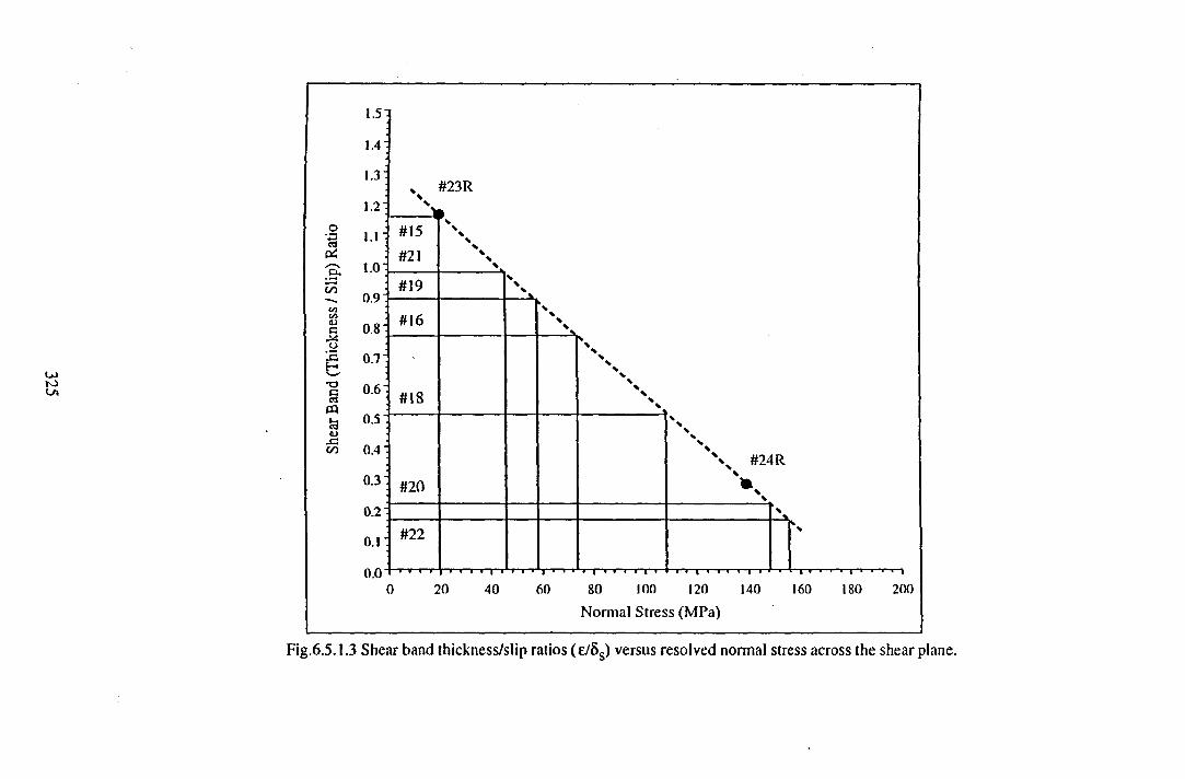
1.51

OJt oU\

oo3

c /5

•occaPQfcs<L)x:

c/o

1.4

1.3

1.2

i . r

l.o-

0.9

0.8

0.7

0.61

0.5

0.4

0.3

0.2

0.1

* #23 R----

#15#21

#19

#16

#1S

#20

#22

X #24R

V

Q Q " j — I— I — i— I— — I — i— i— I— |— i i " i -» |— i — i — |— i — «— I— I— I — i— — I— I— |— a— i— i— i— |— r

0 20 40 60 80 100 120 140 160Normal Stress (MPa)

■ i •» ■ -«• ■ i180 200

Fig.6.5.1.3 Shear band thickness/slip ratios (e/8s) versus resolved normal stress across the shear plane.

thicknesses into Eqn.6.5.1. An indication of fault sealing potential which encompasses

any initial between-sample variations due to microstructural dissimilarities between

specimens, can be gained by normalising each estimate of fault permeability by the

permeability values measured under initial hydrostatic stress conditions. Shear band

permeability estimates and fault sealing potentials (expressed as percentages of hydrostatic

permeabilities) are also given in Table 6.5.1.2.

From Table 6.5.1.2 it is evident that percentage fault sealing potential ranges from 0.35%

at low stress to 0.04% at high stress, representing a 2.5 to 3.5 order o f magnitude

permeability reduction due to cataclasis alone (as the pore fluids were chemically inert, both

hydrolytic weakening and pressure solution are inferred to have been absent). Such

magnitudes are in agreement with outcrop minipermeameter measurements reported by

Antonellini & Aydin (1994)255 on granulation seams in the Navajo and Entrada sandstones

of the Arches National Park, Utah, where, on average, a permeability three orders of

magnitude less than the host rock was quantified. Antonellini & Aydin contended that the

"intensity of cataclasis" and the clay content controlled the amount of permeability reduction

as measured perpendicular to the band, however the minipermeameter method (see for

example Goggin et al, 1988256) is conducted under zero-stress conditions so that

extrapolation of measured magnitudes to reservoir conditions is necessarily tenuous. In

contrast, the Clashach triaxial compression measurements, conducted under stress states

associated with shear slippage, show an order of magnitude dependency on applied stress,

as illustrated in Fig.6.5.1.4 where both estimated shear band permeability (a) and sealing

potential (b) are plotted against normal stress resolved across the fault, giving robust linear

negative correlations. The effect of the main experimental variable, confining pressure, was

also evident in first order control on both fault inclination relative to the direction of the

maximum principal stress, and on shear band thickness, as discussed above. Whilst any

potential influence on permeability of the former additional variable is fully contained

within the geometric constant defined by Eqn.6.5.1.2, the effect of a stress-sensitive shear

band thickness is reflected in a wide between-specimen variability in angular shear strain.

T*. Thus both estimated shear band permeability (a) and sealing potential (b) also show a

strong linear negative correlation with VF, as illustrated in Fig.6.5.1.5. In section 6.5.2

326

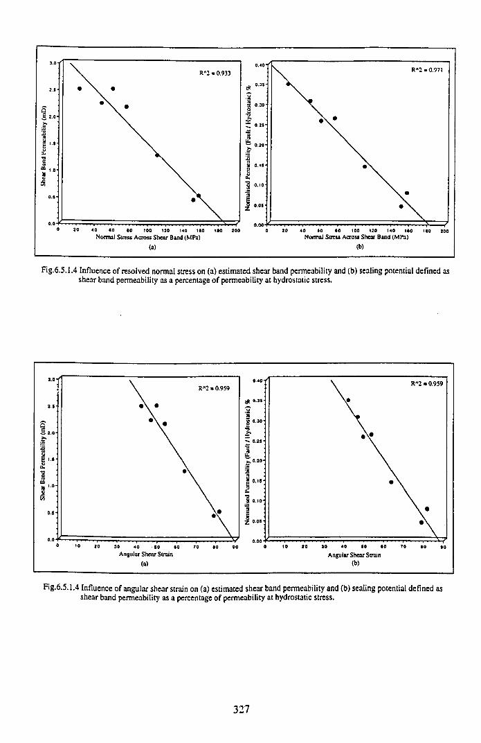
(a) (b)

Fig.6.5.1.4 Influence of resolved normal stress on (a) estimated shear band permeability and (b) sealing potential defined as shear band permeability as a percentage of permeability at hydrostatic stress.

Fig.6.5.1.4 Influence of angular shear strain on (a) estimated shear band permeability and (b) sealing potential defined as shear band permeability as a percentage of permeability at hydrostatic stress.

327

below, the results from laser particle sizing of shear debris recovered from the Clashach

specimens is reported, whilst in section 6.5.3 the "intensity of cataclasis" is quantified in

terms of the Rosin-Rammler constants defining the gouge distributions, and related to the

shear band permeability estimates.

6.5.2 M alvern R esults

Fault gouge samples from the seven Clashach sandstone specimens #15 to #22 were

carefully brushed from the intact specimen halves, and prepared by washing in acetone to

remove excess oil pore fluid, agitating in a sonic bath with distilled water and finally by

oven drying at 100°C for 24hours. The prepared samples were then sieved into >500 and

<500micron fractions, the latter being used for laser particle sizing, suspended in distilled

water as a supporting medium. The optical model employed by the Mastersizer to compute

volume distributions was customised by entering the optical constants o f the sample

material and supporting medium, all the Clashach samples being treated as quartz, with a

refractive index of 1.54. Also, for specific surface area (per g of sample) calculations, all

sample materials were assigned the specific gravity of quartz = 2.65. This approximation of

the fault gouge powders as volume distributions of quartz spheres was thus more realistic

for these Clashach samples than for the direct shear suite, as Clashach sandstone is a quartz

arenite with approximately 90% quartz and no clay fraction. Independent powder samples

from each triaxial compression specimen were analysed using the 300mm- and 45mm-

range lenses, giving particle sizes extending from 600 to 1.2microns and 80 to O.lmicrons

respectively. Unlike the direct shear specimen study, in which the analysis mode was set to

model independent with no assumptions made about the form of the result with regard to its

distribution, for the Clashach suite the Rosin-Rammler two-parameter analysis model was

selected, constraining the volume distribution to have a single peak completely identified by

the two parameters X (describing the position of the peak on the size scale) and N

(describing the width of the distribution) as detailed in section 6.3.

Rewriting the Rosin-Rammler law for the oversize, residual weight distribution

(Eqn.6.2.3.3) in terms of the absolute size constant, x , gives:

328

- ( i ' j "R = 100eA ^ Eqn.6.5.2.1

For n = 1, the peak of the particle size weight distribution curve is theoretically at

R=100eA-l = 100/e = 36.8%, so that if we denote the mode of the distribution curve by x ,

then Eqn.6.5.2.1 becomes, for n = 1 and b = \ ! x , R = 36.8%. The sieve opening .v

corresponding to R = 36.8% is conveniently used as a characteristic o f the degree of

comminution of the material (B e n n e tt^ ) , and since the slope of the straight line on the

Rosin-Rammler graph depends upon the range of particle size, the ratio of the angle a (n =

tana) and the mode x epitomises very effectively the distribution curve as regards both

mode and range of particle size. The quantity ( a / x ) therefore represents a quasi

"coefficient of variation" enabling direct comparison of the degree of dispersion (slope of

the line) in samples from different materials which may possess different modes (position

of the line).

Graphical representation of the Mastersizer Rosin-Rammler particle size distribution

analyses are given in Fig.6.5.2.1(a) and (b), for f=300mm and f=45mm respectively.

Tabulated constants n, a , b, x and ( a l x ) are presented in Table 6.5.2.1. The most

obvious feature of the Rosin-Rammler plots is their extreme linearity, in marked contrast to

those of the model independent volume distributions for the direct shear specimens, when

plotted in the same Rosin-Rammler format. This linearity exhibited by the Clashach

specimens is therefore attributed to the selection of the two-parameter analysis mode,

although it is stressed that this is not unequivocal, as many other contrasts existed between

the two test suites (in particular the mode of testing and associated boundary conditions) so

that no further comparisons will be drawn between the direct shear and triaxial compression

results.

From the particle size distribution plots and tabulated Rosin-Rammler constants, it is

evident that the 300mm-range lens data shows a relatively wide spread in actual particle

329

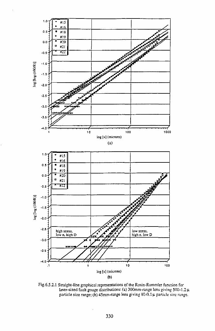
log

[log

(100

/R)]

log

[log

(IflO

/R))

(b)

Fig.6.5.2.I Straight-line graphical representations of the Rosin-Rammier function forlaser-sized fault gouge distributions: (a) 300mm-range lens giving 500-1.2 p particle size range; (b) 45mm-range lens giving 80-0.1 p panicle size range.

330

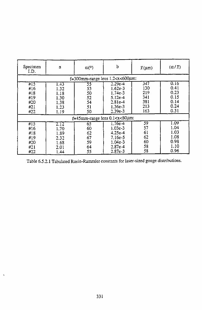
SpecimenI.D.

n a (°) b x(|im ) (a / .r )

f=300mm-range lens 1.2<x<600um:#15 1.43 55 2.29e-4 347 0.16#16 1.32 53 1.62e-3 130 0.41#18 1.18 50 1.74e-3 219 0.23#19 1.30 52 5.12e-4 341 0.15#20 1.38 54 2.81e-4 381 0.14#21 1.23 51 1.36e-3 213 0.24#22 1.19 50 2.39e-3 163 0.31

f=45mm-range lens 0.1<x<80|im:#15 2.12 65 1.76e-4 59 1.09#16 1.70 60 1.03e-3 57 1.04#18 1.89 62 4.25e-4 61 1.03#19 2.32 67 7.16e-5 62 1.08#20 1.68 59 1.04e-3 60 0.98#21 2.01 64 2.87e-4 58 1.10#22 1.44 55 2.87e-3 58 0.96

Table 6.5.2.1 Tabulated Rosin-Rammler constants for laser-sized gouge distributions.

331

size, as denoted by the position of each line, with x ranging from I30microns to

380microns, whilst the between-specimen distribution of particle size remains relatively

constant, with n « 1.3 ± 0.1. In direct contrast, however, the 45mm-range lens data shows

relative uniformity in absolute particle size, x ~ 59 ± 2, whilst the relative distribution of

particle size between Clashach samples, denoted by the slope of each line, shows n ranging

from 1.4 to 2.3. Thus the relatively large size range data (1.2<x<600microns) implies a

wide diversity in the coarseness of the fault gouge from sample to sample, with however all

samples showing the same closeness of grading, whereas the relatively small size range

data (0.1<x<80microns) implies a similar degree of fineness for all samples but a spread in

their individual size reduction characteristic.

In Fig.6.5.2.2, the "coefficient of variation", (a l x ) for both the 300mm- and 45mm-range

lens data is plotted against (a) normal stress resolved across each shear band, crn, and (b)

the total angular shear strain, VF, imposed on each shear band. Strong linear negative

correlations are evident between (cUx) measured on the 45mm-range lens, and both

variables ctn and VF, with critical coefficients, R2 of 0.933 and 0.948 respectively. No such

correlations were evident for the 300mm-range lens data. This correlation for (a / x )

determined on particle size ranging from 80-0.1microns as opposed to the lack of

correlation shown by (a / x ) determined on particle size ranging from 600-1.2microns, may

be attributed to the fact that the lower size range represents 100% cataclastic products,

whereas the larger size range includes both remnant intact grains as well as comminuted

grains. It is evident that for the 45mm-range lens, (a / x ) represents the inverse of

"cataclastic intensity" (x approximately constant, a decreasing with increasing rate of size

reduction) so that the lower the value of the ratio (a l x ) , the more intense the cataclasis.

Marone & Scholz (1989)257 investigated the comminution of simulated fault gouge

(Ottawa sand with >99% quartz) under triaxial compression, between rough steel surfaces

at 45° to the axis o f a cylindrical sample. They found that the fractal dimension, D of the

gouge increased from D =1.6 with increasing shear strain to vF-values of about 52° to 56°,

then levelled off to an asymptotic value of » D =2.8 thereafter (the greater the magnitude of

332

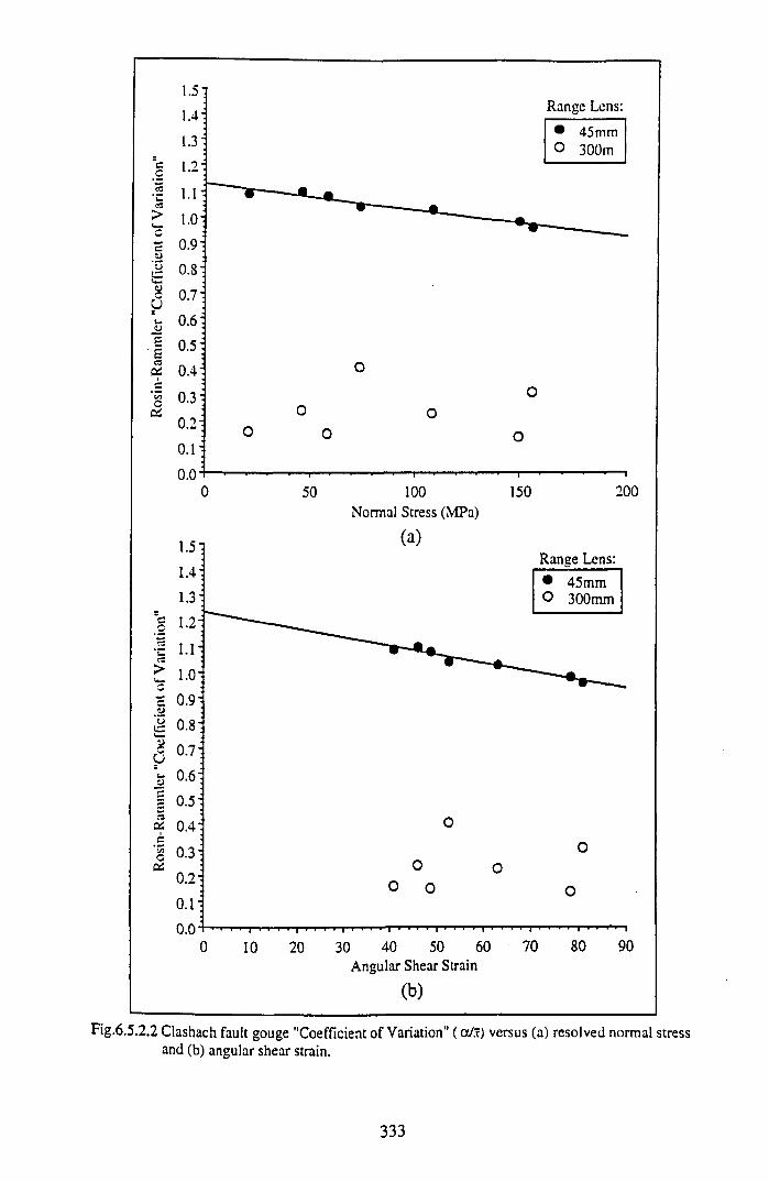
Fig.6.5.2.2 Clashach fault gouge "Coefficient of Variation” ( aJx) versus (a) resolved normal stress and (b) angular shear strain.

333

D, the greater the number of small fragments relative to large fragments). Marone &

Scholz's observation of D increasing with increasing supports the idea that in fact shear

strain represents the primary control on comminution, as all their layer shearing was

conducted at a constant effective normal stress of lOOMPa. However, Sammis et al

found that collected samples of natural fault gouge material from the San Andreas fault zone

showed a linear decrease in mean particle size with increasing confining pressure (depth)

which they attributed to a suppression of microfracture extension and subsequent decrease

in the spacing of axial microfractures with increasing confinement, leading to smaller

particles being produced from denser microfractures at higher pressure. Whilst, with regard

to the Clashach tests, the relative influence of a variable normal stress on frictional

comminution cannot be separated from that of shear strain, the above related studies tend to

suggest that both variables will have a complementary, mutually additive, control on

cataclastic intensity.

Use o f the Rosin-Rammler two-parameter model forces a relationship between the volume

present in each sizeband on the analysis. This two-parameter analysis model uses an

analysis technique to constrain the volume distribution to have a single peak which can be

completely specified by two parameters of the characterising equation, X( = x) describing

the position o f the peak on the size scale, and N (=n) describing the width o f the

distribution. The objective of the two-parameter analysis is to produce a result for which

the residual is a minimum, however if the size distribution is not well represented by the

two-parameter model, a local minima may be found some distance from the true minima,

for example, assuming a value o f X has been found which, if altered by a small amount,

would lead to an increase in the residual, the analysis algorithm takes this to be the best fit

and stops the calculation, however what it cannot predict is that moving the X value by a

large amount may lead to an even lower residual. Thus it is possible that the residual for the

300mm-range lens calculated light energy distribution fit to the measured data may not be

the true residual minimum, but a local one, resulting from a poor fit of the Rosin-Rammler

model to the size distribution. For Clashach sandstone, the particle size range measured by

the 300mm-range lens could include significant contributions from unfractured remnant

grains for gouge developed at relatively low stress levels, whilst the size range accessed by

334

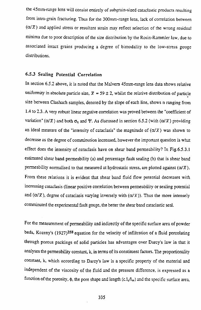
the 45mm-range lens will consist entirely of subgrain-sized cataclastic products resulting

from intra-grain fracturing. Thus for the 300mm-range lens, lack of correlation between

{cUx) and applied stress or resultant strain may reflect selection of the wrong residual

minima due to poor description of the size distribution by the Rosin-Rammler law, due to

associated intact grains producing a degree of bimodality to the low-stress gouge

distributions.

6.5.3 Sealing Potential Correlation

In section 6.5.2 above, it is noted that the Malvern 45mm-range lens data shows relative

uniformity in absolute particle size, x » 59 ± 2, whilst the relative distribution of particle

size between Clashach samples, denoted by the slope of each line, shows n ranging from

1.4 to 2.3. A very robust linear negative correlation was proved between the "coefficient of

variation" (a l x) and both c n and VP. As discussed in section 6.5.2 (with (aJx) providing

an ideal measure of the "intensity of cataclasis" the magnitude of (c/Jx) was shown to

decrease as the degree of comminution increased, however the important question is what

effect does the intensity of cataclasis have on shear band permeability? In Fig.6.5.3.1

estimated shear band permeability (a) and percentage fault sealing (b) that is shear band

permeability normalised to that measured at hydrostatic stress, are plotted against (oc/Jc).

From these relations it is evident that shear band fluid flow potential decreases with

increasing cataclasis (linear positive correlation between permeability or sealing potential

and (a lx), degree of cataclasis varying inversely with (a lx)). Thus the more intensely

comminuted the experimental fault gouge, the better the shear band cataclastic seal.

For the measurement of permeability and indirectly of the specific surface area of powder

beds, Kozeny's (1927)2S8 equation for the velocity of infiltration of a fluid percolating

through porous packings of solid particles has advantages over Darcy's law in that it

analyses the permeability constant, k, in terms of its constituent factors. The proportionality

constant, k, which according to Darcy's law is a specific property of the material and

independent of the viscosity of the fluid and the pressure difference, is expressed as a

function of the porosity, <)), the pore shape and length (c.ls/lw) and the specific surface area,

335

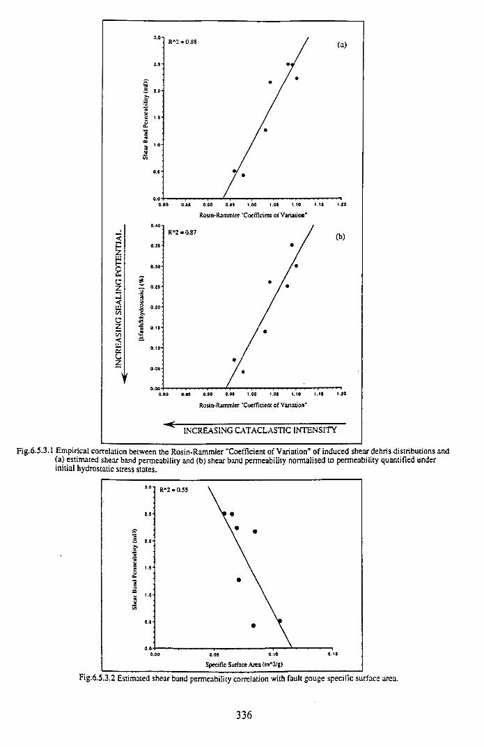
<P2££c2

<UcnC2t / i<luCiU2

y

INCREASING CATACLASTIC INTENSITY

Fig.6.5.3.1 Empirical correlation between the Rosin-Rammler "Coefficient of Variation" of induced shear debris distributions and (a) estimated shear band permeability and (b) shear band permeability normalised to permeability quantified under initial hydrostatic stress states.

Fig.6.5.3.2 Estimated shear band permeability correlation with fault gouge specific surface area.

336

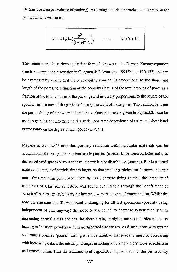
Sv (surface area per volume of packing). Assuming spherical particles, the expression for

permeability is written as:

k — (c. Is / lw)( i - * ) 2

Eqn.6.5.3.1

This relation and its various equivalent forms is known as the Carman-Kozeny equation

(see for example the discussion in Gueguen & Palciauskas, 1994-^, pp. 126-133) and can

be expressed by saying that the permeability constant is proportional to the shape and

length of the pores, to a function of the porosity (that is of the total amount of pores as a

fraction of the total volume of the packing) and inversely proportional to the square of the

specific surface area of the particles forming the walls of those pores. This relation between

the permeability of a powder bed and the various parameters given in Eqn.6.5.3.1 can be

used to gain insight into the empirically demonstrated dependence of estimated shear band

permeability on the degree of fault gouge cataclasis.

Marone & Scholz257 note that porosity reduction within granular materials can be

accommodated through either an increase in packing (a better fit between particles and thus

decreased void space) or by a change in particle size distribution (sorting). For less sorted

material the range of particle sizes is larger, so that smaller particles can fit between larger

ones, thus reducing pore space. From the laser particle sizing studies, the intensity of

cataclasis o f Clashach sandstone was found quantifiable through the "coefficient of

variation" parameter, ( a / x ) varying inversely with the degree of comminution. Whilst the

absolute size constant, x , was found unchanging for all test specimens (porosity being

independent of size anyway) the slope ot was found to decrease systematically with

increasing normal stress and angular shear strain, implying more rapid size reduction

leading to "dustier" powders with more dispersed size ranges. As distributions with greater

size ranges possess "poorer" sorting it is thus intuitive that porosity must be decreasing

with increasing cataclastic intensity, changes in sorting occurring via particle-size reduction

and comminution. Thus the relationship of Fig.6.5.3.1 may well reflect the permeability

337

versus porosity relationship of Eqn.6.5.3.1 with fluid flow potential increasing with

improved sorting. Also, it is possible that increased normal stress across the shear band

may have the added effect of increasing compaction within the gouge zone, hence

promoting grain-packing in addition to sorting as a mechanism for porosity reduction.

In Fig.6.5.3.2, shear band permeability is plotted as a function of the specific weight

surface area. Sw = Sv/p, calculated from the harmonic mean of the weight distribution -

volume surface diameter equivalency. A linear negative trend is evident, indicating that, as

well as the presumed decrease in porosity with increasing comminution, increasing fault

gouge specific area also decreases shear band permeability, as predicted by Eqn.6.5.3.1. It

is also likely that tortuosity (defined as the ratio of real to apparent path length through

which the fluid flows, lw/ls) will also increase with increasing cataclasis, with an attendant

inverse effect on permeability magnitude.

338

7. EXPERIM ENTAL CONCLUSIONS AND FURTHERANCE OF W ORK

7.1 CONCLUSIONS

7.1.1 Direct Shear Experim entation

(i) A servo-hydraulic direct shear rig has successfully been used to shear whole core

(118mm-diameter) rock specimens of diverse sedimentary lithology under

constant normal displacement (CND) control, analogous to "ultra-stiff' wall-rock

in situ boundary conditions.

(ii) Consequences of the CND experimental boundary conditions include maximum

suppression of discontinuity-normal displacement and maximum production of

frictional wear debris (fault gouge).

(iii) Macroscopic specimen deformation under CND conditions was observed to be

markedly lithology-dependent. Four rock types were tested, including Permian red

sandstone and Carboniferous fissile mudstone, carbonaceous siltstone and

heterolithics, and exhibited widely different discontinuity deformation modes with

regard to sliding surface morphology and shear debris production.

(iv) All CND direct shear specimens showed sliding surface structures analogous to

those observed on natural faults and used as kinematic indicators (shear sense

criteria). Specifically, well-developed slickensides, slickenlines and slickensteps

were apparent, the latter being observed to face against the movement direction of

the overriding block, in agreement with current structural geological

interpretation.

(v) Force-displacement curves for CND-shear showed sudden distinct stress drops

which were interpreted as being due to asperity shear.

(vi) Theoretical analysis of contact area variation with sliding displacement was

undertaken, based geometrically on the area of overlap of two circles with

divergent centre displacement. Incorporation of slip-dependent contact area into

shear and normal stress magnitude calculations from measured loads was shown

to have a first order influence on stress versus sliding displacement profiles, by

comparison with those based on the assumption of constant contact area.

339

(vii) Each CND specimen showed a distinct peak in its shear load versus displacement

profile which was used to define a maximum friction coefficient, | imax, equal to

the peak shear stress divided by the corresponding normal stress. Direct shear

maximum friction data consistently plotted below Byerlee's low normal stress

(a n<200MPa) frictional strength relationship, x=0.85cn, and was better

represented by the high normal stress relationship, x = 0.5+0.6crn. This may reflect

the suppression of dilatancy under CND conditions, where asperity shear is

wholly dominant, and highlights discontinuity stiffness as an important omission

with regard to Byerlee's hypothesis.

(viii) The variable friction coefficient, |i*=x/an was seen to decrease with increasing

normal stress due to surface wear associated with CND shearing, indicating that

Amonton’s law as defined above is invalid for the various rock types tested under

the experimental direct shear configuration.

(ix) In shear stress versus normal stress space, all lithologies exhibited the same

overall attributes irrespective of lithology, namely a non-linear (generally

exponential) increase in pre-peak strength data to maximum friction, p.max,

followed by post-peak data which exhibits a robust linear trend determined by a

slope (designated the coefficient of sliding friction, Ps) and an intercept

(designated the inherent cohesion of the contact surfaces, S0).

(x) From empirical observations detailed in (ix) above, direct shearing of sedimentary

rocks under CND boundary conditions is thus envisaged as a two stage process

associated with pre- and post-maximum friction deformation modes: In physical

terms maximum friction represents peak shear strength of the macroscopic

discontinuity, immediately prior to through-going breaching of the interlocking

asperity system, followed by "residual" frictional sliding on a newly-created

pervasive shear plane with a substrate of frictional wear debris. Thus for CND

boundary conditions it appears that two coefficients of friction are relevant: the

first, (imax, relates to the process of actually creating the slip surface through the

interlocking asperities, whilst the second, p.s, relates to slip on the resultant

pervasive, freshly fractured shear plane and associated wear products.

340

7.1.2 Triaxial Compression Experim entation

(i) A combined microseismics monitoring and liquid permeability measurement

facility has successfully been coupled to a conventional rock mechanical triaxial

compression system. Thus shear bands (morphologically similar to natural

"granulation seams") induced under confining pressures equivalent to overburden

depths ranging from 0.3km to 3km, have been studied with regard to synchronous

measurement of acoustic emissions associated with post-failure frictional sliding

deformation, and fault sealing potential associated with cataclasis.

(ii) The test reservoir sandstone analogue (Permo-Triassic Clashach sandstone, a

coarse-grained subarkosic arenite with approximately 90% quartz and 10%

feldspar) exhibits a curvilinear fracture strength envelope, better represented by

the parabolic Griffith law than the linear Mohr-Coulomb criterion. Physically, this

manifests itself in a stress-sensitive fault inclination, with the angle 0, between the

shear band and the direction of maximum compressive stress increasing frrom 20°

to 40° with increasing confining pressure.

(in) Discrete, pulse-decay liquid (refined mineral oil) permeabilities have been

measured at stress states corresponding to hydrostatic, post-dynamic failure, post-

frictional sliding and post-re-shearing following artificial mechanical

strengthening conditions, under a drained environment with pore pressure being

equal to atmospheric. Experimental relative error on each individual permeability

measurement was calculated to be probably not larger than ±10%.

(iv) Axial permeability measurements showed no systematic correlation with

hydrostatic stress magnitude. This was interpreted as being due to the fact that, for

the relatively porous and strong Clashach sandstone, increasing hydrostatic stress

led to quasi-elastic decrease in pore diameter, with however no lowering of pore

space connectivity.

(v) In contrast, post-macroscopic shear failure, axial permeability showed a

pronounced linear decrease in magnitude with increasing normal stress resolved

across the shear band. The overall permeability drop with increasing stress, and

the correlation coefficient of the linear fit, both increased with increasing shear

displacement, that is from immediate post-failure to post-re-shear conditions. For

341

the latter situation, axial permeability decreased 100% with increasing resolved

normal stress.

(vi) For the initial high-permeability Clashach sandstone (at hydrostatic stress, of the

order of 1 Darcy) for which the assumption of shear band permeability being very

much less than that of the stressed rock matrix is valid (implying that virtually all

of the measured pressure drop across the specimen actually occurs across the

shear band) a simple empirical expression is derived which equates the measured

core plug permeability to the product of a geometric constant (defined below) the

shear band permeability, and the inverse of the shear band thickness.

(vii) With the geometric constant as described in (vi) above and defined as the product

of core length, fault plane area and the inverse of the core plug cross-sectional

area, also showing a linear decrease with increasing resolved normal stress (due to

fault inclination stress sensitivity as defined in conclusion (ii) above) it is evident

that shear band permeability dependence on the applied stress state cannot be

inferred from axial permeability correlations alone.

(viii) Three-stage acoustic emission (AE) monitoring has allowed temporal variation in

event rate, seismic b-value and inferred fractal dimension, D, to be determined for

transient triaxial stresses increasing from hydrostatic to immediate post-dynamic

failure conditions, for frictional sliding and for re-shearing on mechanical

strengthening. This was achieved using a novel waveguide designed specifically

for coupling a receiver transducer with rock core confined within a conventional

Hoek-type hydraulic pressure vessel.

(ix) For stress histories involving triaxial loading from hydrostatic conditions to those

associated with compressional failure in macroscopic shear, AE activity was seen

to conform to an existing semi-quantitative, synoptic fractal damage mechanics

model for brittle failure of intact laboratory specimens. Over the complete stress-

strain curve, this model predicts transients in the seismic b-value and thus an

"instantaneous" fractal dimension (D =2b). Fractal dimension was observed to

range in magnitude from D >2 (b>l) associated with quasi-elastic loading to D =1

(b=0.5) at dynamic failure, corroborating the idea of rock failure in compression

by shear faulting, being preceded by a phase of tensile microcrack nucleation,

342

growth and coalescence, associated with positive (D <2) or negative (D >2)

feedback in local stress concentration during deformation.

(x) AE generated under conditions of post-peak slip-weakening, gave time-varying

seismically inferred D -values of remarkably constant magnitude « 2,

characteristic of random processes (for example cataclastic flow) despite large

spikes in event rate inferred to be the result of asperity shearing . On mechanical

strengthening through a transient increase in confinement, this D -value remained

unchanged, in direct contrast to the large fluctuations observed during the

nucléation stage of faulting. This stability in the power law scaling exponent,

combined with a relatively constant driving stress at constant strain rate, implies

that frictional sliding conforms to a self-organised critical (SOC) phenomenon,

consistent with recent treatment of crustal faulting, and suggests that fault-wall

roughening processes are occurring synchronously with gouge comminution.

7.1.3 Experimental Fault Gouge Analyses

(i) Empirical correlations were demonstrated between the Rosin-Rammler constants

of the relatively large-sized direct shear debris distributions quantified by sieving

analysis, and percentage mineral content of the host multilithologic specimens. In

particular, the distribution constant relation (n decreasing with increasing clay

content) was interpreted to be a result of the influence of rock type on strain

accommodation at the microscale, with the relative amounts of shearing

fragmentation to tensile cracking being reflected in the resultant debris

distributions.

(ii) Laser particle sizing techniques were successfully applied to both experimental

direct shear and triaxial compression frictional wear products, over particle size

ranges of 600-1.2 and 80-0.1 microns, depending on the experimental

configuration and optical model employed. In general, good correlation was

evident between the sieving and laser sizing results over the appropriate size

range.

(iü) With the slope of the log-normal curve providing an indication of particle sorting,

a general trend was evident for the quartz-rich/clay-poor samples where a change

343

in sorting was evident at around 0 .1mm particle size, which may reflect a gouge

microstructure composed of relatively well-sorted, intact remnant grains within a

fine-grained, comminuted matrix representing steady-state size reduction down to

the limits of size resolution. In contrast, the clay-rich/quartz-poor samples exhibit

strongly sigmoidal curves and a minimum comminution limit of about 1 micron.

This observation indicates that the comminution efficiency of the clay-rich

specimens is reduced at small particle size, compared to that of the quartz-rich

specimens, which may reflect the nature of the inter-particle stress concentrations

for the different mineral phases.

(iv) Fault gouge fractal dimensions were generated from the linear portions of the

Rosin-Rammler plots, utilising the relation D =3-n. The magnitude of D was

found to be 1.5<D <2.4 and 1.7<D <2.2 for the 600-1.2 and 80-0.1micron size

ranges respectively, in keeping with the range of published magnitudes for diverse

fragmentation phenomena.

(v) A moderate empirical correlation was demonstrated between fault gouge fractal

dimension and the coefficient of sliding friction, reflecting the direct relation

between fractal dimension and specific surface area (surface area per unit mass of

powder) as higher D -values indicate a higher number of small relative to large

fragments. Linear positive correlation between specific surface area and the

coefficient of sliding friction (also empirically demonstrated) may reflect an

increase in frictional resistance associated with an increase in the energy required

to create new surface area.

(vi) Shear fracture energies, Gnc. were estimated for those direct shear experiments in

which slip-weakening behaviour was evident, of magnitude Gnc = 0-1-1.5 x

104Jm*2. Constant normal displacement direct shear testing gives Gnc*values four

orders of magnitude greater than published biaxial tests under controlled constant

normal stresses of equivalent measure, and of the same order of magnitude as

triaxial compression tests conducted under considerably higher normal stresses,

due to the greater degree of brecciation resulting from direct shear under

maximum normal stiffness conditions, despite associated normal stresses

<10MPa. Thus it is possible that in situ boundary conditions may provide an

344

answer to the discrepancy between the maximum laboratory measured values of

shear fracture energy and field estimates for natural faults from seismological

data.

(vii) Logarithmic positive empirical correlations have been demonstrated between

shear fracture energy and both fault gouge specific surface area and fractal

dimension, implying that increasing fracture resistance is associated with an

increase in comminution (surface energy) as a proportion of the total energy

dissipation process behind the rupture front. A logarithmic positive empirical

correlation is also evident between the shear fracture energy and the coefficient of

sliding friction.

(viii) From resin-impregnated thin-section photomicrographs of Clashach sandstone

faulted triaxial specimens, shear band thickness and wall-rock roughness were

both observed to decrease with increasing resolved normal stress, in direct

contrast to an existing steady-state wear law developed for non-porous substrates

with the assumption of zero fault gouge porosity change with compaction. At low

normal stress magnitudes, both grain-boundary sliding and intra-granular

fracturing contribute to the cataclastic deformation, whereas at high normal

stresses, the latter mechanism dominates the cataclastic process.

(ix) For the assumption of a linear decrease in thicknessrslip ratio with increasing

normal stress (calibrated from thin-section measurement of two control

specimens) Clashach sandstone experimentally induced shear bands were

calculated to have absolute permeabilities ranging from approximately 2.5mD

down to 0.5mD with increasing normal stress and angular shear strain.

Normalised to permeability measured on the intact sample under hydrostatic

stress conditions, these shear band permeability magnitudes equate to a "fault

sealing potential" ranging from 0.35 to 0.04%. Thus computed permeability

reductions range from 2.5 to 3.5 orders of magnitude, with shear band sealing

exhibiting an order of magnitude increase with increasing normal stress and

angular shear strain imposed on the gouge zone.

(x) Laser particle sizing was used to define the peak (relative fineness) and width of

distribution (closeness of grading) of the fault gouge samples generated by the

345

above mentioned shear bands, through application of the exponential Rosin-

Rammler distribution function, which was able to quantify "cataclastic intensity"

via a "coefficient of variation" statistical parameter. The Rosin-Rammler

coefficient of variation showed linear decrease (implying increasing cataclastic

intensity) with increasing normal stress and angular shear strain, and a robust

linear correlation with fault sealing potential was demonstrated, indicating that the

effectiveness of cataclastic sealing as a fluid baffle decreases as the degree of fault

gouge comminution decreases.

(xi) This empirical relation demonstrated between fault seal and degree of cataclasis

can be rationalised through consideration of the Kozeny-Carman relation, which

analyses permeability in terms of its constituent parameters of, porosity, surface

area and tortuosity. An empirical linear negative correlation between estimated

shear band permeability and fault gouge specific surface area was proven, as

predicted by the Kozeny-Carman relation

7.2 FURTHER W ORK

7.2.1 Direct Shear Experimentation

(i) Equipment development should concentrate on the provision of confining

pressure for the direct shear specimens, so that comparison can be made between

shear under constant normal stress and displacement boundary conditions at

reservoir stress magnitudes. A coupled pore pressure and permeameter system

would enable fault seal potential to be directly measured under stress histories

associated with production.

(ii) AE monitoring of the direct shear programme would enable fractal damage

' mechanics to be applied to greater sliding displacement events. AE statistics

could be used to provide a suitable basis on which to build a micromechanical

theory of rock friction, and to assess the influence of boundary conditions on

frictional sliding.

346

7.2.2 Triaxial Compression Experimentation

(i) Post-mortem analysis of sandstone specimens sheared under triaxial compression

conditions, involving small particle statistics combined with wall-rock surface

roughness measurement, would allow a frictional wear law relating thickness,

wear loss, stress and displacement to be developed for porous reservoir rock.

(ii) The addition of finite pore pressures would enable investigation of the influence

of effective stresses and degrees of overpressurisation on cataclastic seal integrity

and on fault gouge statistics.

7.2.3 Experimental Fault Gouge Analyses

(i) As well as aiding in the understanding of fault-sealing by cataclasis, the ability to

quantify comminution products through laser particle sizing and small particle

statistics has great potential in the hydrocarbon industry, including study of the

"crush" characteristics of proppant used to wedge open hydraulic fractures, and

the problem of sand production from producing wells, where local shear stresses

have exceeded rock strength in the vicinity of the wellbore.

(ii) The strain energy expended in creating new surface area (fault gouge) should be

quantified under constant normal displacement boundary conditions and

expressed as a percentage of the total work done in sliding. This value can then be

contrasted with that obtained from constant normal stress tests.

347

REFERENCES

CHAPTER 1

[1] Rutter, E.H. 1986. On the nomenclature of mode of failure transitions in rocks.

Tectonophysics Vol. 122. pp.381-387.

[2] Knipe, R.J. 1989. Deformation mechanisms - recognition from natural tectonites.

J. Struct. Geol. Vol. 1. No. 2. pp. 127-146.

[3] Maltman, A. 1984. On the term "soft sediment" deformation. J. Struct. Geol. Vol.

6. pp.589-592.

[4] Wang, C.H. 1986. Internal structure of fault zones. Pure & Appl. Geophys. Vol.

124. pp.373.

[5] Knipe, R.J. 1986. Microstructural evolution of vein arrays preserved in D.S.D.P.

cores from Japan Trench Leg 57. In: Structural Fabrics In D.S.D.P. Cores from

Forearcs. Moore, J.M. (Ed.) Mem. Geol. Soc. Am. 166. pp.75-88.

[6] Coulomb, C.A. 1773. Sur une application des règles de Maximis et Minimis a

quelques problèmes de statique relatifs à l'Architecture. Acad. Roy. des Sciences

Mémoires de math, et de physique par divers savans. Vol. 7. pp.343-382.

[7] Mohr, O. 1900. Welche Umstande bedingen die Elastizitätsgrenze und den Bruch

eines Materials? Z Ver. dt. Ing. Vol. 44. pp. 1524-1530; 1572-1577.

[8] Jaeger, J.C. & Cook, N.G.W. 1979. Fundamentals of Rock Mechanics . (3rd.

Edn.) Chapman & Hall. London. 593pages.

[9] Paterson, M.S. 1978. Experimental Rock Deformation - The Brittle Field.

Springer Verlag. Berlin. 254p.

[10] Mohr, O. 1914. Abhandlungen aus dem Gebiete der technische Mechanik (2nd.

Edn.) Emst und Sohn, Berlin.

[11] Griggs, D.T. & Handin, J. 1960. Observations on fracture and an hypothesis of

earthquakes. In: Rock Deformation, Geol. Soc. Am. Mem. Vol. 79. pp.39-104.

[12] Anderson, E.M. 1951. The Dynamics of Faulting and Dyke Formation with

Applications to Britain. (2nd. Edn.) Oliver & Boyd. Edinburgh.

348

[13] Sibson, R.H. 1973. Interaction between temperature and pore-fluid pressure during

earthquake faulting - a mechanism for partial or total stress relief. Nature Phys. Sci.

Vol. 243. pp.66-88.

[14] Griffith, A.A. 1920. The phenomena of rupture and flow in solids. Phil. Trans. R.

Soc. Ser. A. Vol. 221. pp. 163-198.

[15] Sneddon, I.N. 1946. The distribution of stress in the neighbourhood of a crack in an

elastic solid. Proc. R. Soc., London. Vol. 187 A. pp.229-260.

[16] Scholz, C.H. 1990. The Mechanics of Earthquakes and Faulting. Cambridge

University Press. Cambridge. 439pages.

[17] Griffith, A.A. 1924. The Theory of Rupture. In: Proc. 1st. Int. Congr. Appl. Mech.

Biezeno, C.B. & Burgers, J.M. (ed.’s) Delft. Tech. Boekhandel en Drukkerij. J.

Waltman Jr. pp.54-63.

[18] Brace, W.F. & Bombolakis, E.G. 1963. A note on brittle crack growth in

compression. J. Geophys. Res. Vol. 68. pp.3709-3713.

[19] Orowan, E. & Nog, The N., 1949. Fracture and Strength of Solids. Rep. Prog. Phys.

Vol. 12. pp. 185-232.

[20] Murrell, S.A.F. 1958. The strength of coal under triaxial compression. In:

Mechanical Properties o f Non-metallic Brittle Materials. Walton, W.H. (ed.)

Buterworths. London, pp. 123-145.

[21] Murrell, S.A.F. 1963. A criterion for brittle fracture of rocks and concrete under

triaxial stress, and the effect of pore pressure on the criterion. In: Fairhurst, C. (ed.)

Rock Mechanics. Proc. 5th. Symp. Rock Mech. Pergamon Press. N.Y. pp.563-577.

[22] Murrell, S.A.F. 1965. The effect of triaxial stress systems on the strength of rocks

at atmospheric temperatures. Geophys. J. Roy. Astr. Soc. Vol. 10. pp.231-281.

[23] McLintock, F.A. & Walsh, J.B. 1962. Friction on Griffith cracks in rocks under

pressure. In: Proc. 4th. U.S. Nat. Congr. Appl. Mech. Vol. II. Am. Soc. Mech. Eng.

N.Y. pp. 1015-1021.

349

[24] Murrell, S.A.F. & Digby, P.J. 1970. The theory of brittle fracture initiation under

triaxial stress conditions. I. Geophys. J. Roy. Astr. Soc. Vol.19. pp.309-334; II. ibid.

pp.499-512.

[25] Brace, W.F. 1960. An extension of the Griffith theory of fracture to rocks. J.

Geophys. Res. Vol.65. pp.3477-3480.

[26] Price, N.J. & Cosgrove, J.W. 1990. Analysis of Geological Structures Cambridge

University Press. 502pages.

[27] Irwin, G.R. 1958. Fracture In: Flügge, S. (ed.) Handbuch der Physik Vol.VI.

Elastizität und Plastizität. Springer-Verlag. Berlin, pp.551-590.

[28] Atkinson, B.K. 1987. Introduction to fracture mechanics and its geophysical

applications. In: Atkinson, B.K. (ed.) Fracture Mechanics of Rock Academic

Press. London, pp.1-26.

[29] Irwin, G.R. & de Wit, R. 1983. J. Testing & Evaluation. V ol.ll. pp.56-65.

[30] ISRM Suggested Methods for Determining the Fracture Toughness of Rock. 1988.

Ouchterlony, F. (Co-ordinator). Int. J. Rock Mech. Min. Sei. & Geomech. Abstr.

Vol.25.No.2 pp.71-96.

[31] Li, V.C. 1987. Mechanics of shear rupture applied to earthquake zones. In:

Atkinson, B.K. (ed.) Fracture Mechanics o f Rock Academic Press. London.

pp.351-428.

[32] Santarelli, F.J. & Brown, E.T. 1989. Failure of three sedimentary rocks in triaxial

and hollow cylinder compression tests. Int. J. Rock Mech. Min. Sei. & Geomech.

Abstr. Vol.26. No.5 pp.401-413.

[33] Hallbauer, D.K., Wagner, H., & Cook, N.G.W. 1973. Some observations

concerning the microscopic and mechanical behaviour of quartzite specimens in

stiff, triaxial compression tests. Int. J. Rock Mech. Min. Sei. & Geomech. Abstr.

Vol.10. pp.713-726.

[34] Brace, W.F. 1964. Brittle fracture of rocks. In: Judd, W.R. (ed.) State of Stress In

the Earth's Crust Elsevier. N.Y. pp. 111-174.

350

[35] Brace, W.F., Paulding, B.W. & Scholz, C.H. 1966. Dilatancy in the fracture of

crystalline rocks. J. Geophys. Res. Vol.71. pp.3939-3953.

[36] Bieniawski, Z.T. 1967. Mechanism of brittle fracture of rock. Part I. Theory of the

fracture process; Part II. Experimental studies; Part III. Fracture in tension and

under long-term loading, Int. J. Rock Mech. Min. Sci. Vol.4. pp.395-430.

[37] Walsh, J.B. 1965. The effect of cracks on the uniaxial elastic compression of rocks.

J. Geophys. Res. Vol. 70. pp.399-411.

[38] Sobolev, G., Spetzler, H. & Salov, B. 1978. Precursors to failure in rocks while

undergoing anelastic deformations. J. Geophys. Res. Vol.83. pp. 1775-1784.

[39] Hadizadeh, J. & Rutter, E.H. 1983. The low temperature brittle-ductile transition in

a quartzite and the occurrence of cataclastic flow in nature. Geologische Rundschau

Vol.72. No.2. pp.493-509.

[40] Cox, S.J.D. & Scholz, C.H. 1988. On the formation and growth of faults: an

experimental study. J. Struct. Geol. Vol. 10. No.4. pp.413-430.

CHAPTER 2

[41] Aguilera, A. 1980. Naturally Fractured Reservoirs . Petroleum Publishing Co.

Tulsa, Oklahoma.

[42] Heath, A.E., Walsh, J.J., & Watterson, J. 1994. Estimation of the effects of sub-

seismic sealing faults on effective permeabilities in sandstone reservoirs. In: Aasen,

J.O., Berg, E., Buller, A.T., Hjelmeland, O., Holt, R.M., Kleppe, J. & Torsaeter, O.

(ed.'s) North Sea Oil & Gas Reservoirs - III. Norwegian Institute of Technology

(NTH). Kluwer Academic Publishers. Dordrecht, pp. 173-183.

[43] Childs, C., Walsh, J.J. & Watterson, J. 1990. A method for estimation of the

density of fault displacements below the limits of seismic resolution in reservoir

formations. In: Buller, A.T., Berg, E., Hjelmeland, O., Kleppe, J., Torsaeter, O. &

Aasen, J.O. (ed.'s) North Sea Oil & Gas Reservoirs - II. Graham & Trotman.

London, pp.309-318.

351

[44] Heffer, K.J. & Bevan, T.G. 1990. Scaling relationships in natural fractures - data,

theory and applications. SPE 20981. Proc. EUROPEC '90 The Hague. Netherlands.

pp.367-376.

[45] Yielding, G., Walsh, J.J. & Watterson, J. 1992. The prediction of small-scale

faulting in reservoirs. First Break Vol.10. pp.449-460.

[46] Walsh, J.J., Watterson, J, & Yielding, G. 1994. Determination and interpretation of

fault size populations: procedures and problems. In: Aasen, J.O., Berg, E., Buller,

A.T., Hjelmeland, 0 ., Holt, R.M., Kleppe, J. & Torsaeter, O. (ed.'s) North Sea Oil

& Gas Reservoirs - III. Norwegian Institute of Technology (NTH). Kluwer

Academic Publishers. Dordrecht, pp. 141-155.

[47] Knott, S.D. 1993. Fault seal analysis in the North Sea. Bull. Am. Assoc. Pet. Geol.

Vol.77. No.5. pp.778-792.

[48] Marrett, R. & Allmendinger, R.W. 1991. Estimates of strain due to brittle faulting:

sampling of fault populations. J. Struct. Geol. Vol.13. No.6. pp.735-738.

[49] Allegre, C.J., Le Mouel, J.L. & Provosi, A. 1982. Scaling rules in rock fracture and

possible implications for earthquake prediction. Nature Vol.297. pp.47-49.

[50] Haldorsen, H.H. & Lake, L.W. 1984. A new approach to shale management in

field-scale models. J. Soc. Pet. Eng. pp.447-457.

[51] Begg, S.H. & King, P.R. 1985. Modelling the effects of shales on reservoir

performance: calculation of effective vertical permeability. SPE 13539.

[52] Holden, L., Hoiberg, J. & Lia, O. 1990. An estimator for the effective permeability.

In: Guerillo, D. & Guillon, O. (ed.'s) 2nd. Eur. Conf. On the Mathematics of Oil

Recovery. Editions Technip. Paris, pp.287-290.

[53] Knipe, R.J. 1992. Faulting processes and fault seal. In: Larsen, R.M., Brekke, H.,

Larsen, B.T. & Talleras, E. (ed.'s) Structural and Tectonic Modelling and its

Application to Petroleum Geology. Norwegian Petroleum Society (NPF) Special

Publication 1. Elsevier. Amsterdam, pp.325-342.

[54] Hubbert, M.K. 1953. Entrapment of petroleum under hydrodynamic conditions.

Bull. Am. Assoc. Pet. Geol. Vol. 37. pp. 1954-2026.

352

[55] Watts, N.L. 1987. Theoretical aspects of cap-rock and fault seals for single and

two-phase hydrocarbon columns. Mar. Pet. Geol. Vol.4. pp.274-307.

[56] Berg, R.R. 1975. Capillary pressure in stratigraphic traps. Bull. Am. Assoc. Pet.

Geol. Vol. 59. pp.939-956.

[57] Sibson, R.H. 1981. Fluid flow accompanying faulting: field evidence and models.

In: Simpson, D.W. & Richards, P.G. (ed.'s) Earthquake Prediction: An

International Review. Am. Geophys. Union. M. Ewing Ser. Vol. 4. pp.593-603.

[58] Sibson, R.H. 1990. Conditions of fault-valve behaviour. In: Knipe, R.J. & Rutter,

E.H. (ed.'s) Deformation Mechanisms, Rheology and Tectonics.. Geological Society

Special Publication No. 54. London, pp. 15-28.

[59] Burley, S.D., Mullís, J. & Matter, A. 1989. Timing diagenesis in the Tartan

Reservoir (UK North Sea): constraints from combined cathodoluminescence

microscopy and fluid inclusion studies. Mar. Pet. Geol. Vol. 6. No. 2. pp.98-120.

[60] Sibson, R.H. 1985. Stopping of earthquake ruptures at dilation fault jogs. Nature

Vol. 316. pp.248-251.

[61] Sibson, R.H. 1986. Brecciation processes in fault zones - inferences from

earthquake rupturing. Pur. Appl. Geophysics. Vol. 124. pp. 159-175.

[62] Smith, D.A. 1980. Sealing and non-sealing faults in the Louisiana Gulf Coast

Basin. Bull. Am. Assoc. Pet. Geol. Vol. 64. pp. 145-172.

[63] Weber, K.J., Mandl, G., Pilaar, W.F., Lehner, F. & Precious, R.G. 1978. The role

of faults in hydrocarbon migration and trapping in Nigerian growth fault structures.

SPE Proc. 10th Annual Offshore Technology Conference. Vol. 4. pp.2643-2653.

[64] Lindsay, N.G., Murphy, F.C., Walsh, J.J. & Watterson, J. 1993. Outcrop studies of

shale smears on fault surfaces. In: Flint, S.S. & Bryant, I.D. (ed.’s) The Geological

Modelling of Hydrocarbon Reservoirs and Outcrop Analogues. Spec. Publ.

Int. Assoc, of Sedimentologists. Vol. 15. pp. 113-124.

[65] Ramsay, J.G. 1980. Shear zone geometry: a review. J. Struct. Geol. Vol. 2. pp.83-

89.

353

[66] Ramsay, J.G. & Huber, M.I. 1983. The Techniques of Modem Structural Geology

Vol. I: Strain Analysis. Academic Press Inc. London. 307pages.

[67] Barnett, J.A.M., Mortimer, J., Rippon, J.H., Walsh, J.J., & Watterson, J. 1987.

Displacement geometry in the volume containing a single normal fault. Bull. Am.

Assoc. Pet. Geol. Vol. 71. pp.925-937.

[68] Mandl, G., de Jong, L.N.J. & Maltha, A. 1977. Shear zones in granular material.

Rock Mechanics Vol. 9. pp.95-144.

[69] Engelder, J.T. 1974. Cataclasis and the generation of fault gouge. Geological

Society of America Bulletin . Vol. 85. pp. 1515-1522.

[70] Ay din, A. 1978. Small faults formed as deformation bands in sandstone. Pure Appl.

Geophys. Vol. 116. pp.913-930.

[71] Pittman, E.D. 1981. Effect of fault-related granulation on porosity and permeability

of quartz sandstones; Simpson Group (Ordovician), Oklahoma. Bull. Am. Assoc.

Pet. Geol. Vol. 65. pp.2381-2387.

[72] Jamison, W.R. & Steams, D.W. 1982. Tectonic deformation of Wingate Sandstone.

Colorado National Monument. Bull. Am. Assoc. Pet. Geol. Vol. 66. pp.2584-2608.

[73] Blenkinsop, T.G. & Rutter, E.H. 1986. Cataclastic deformation of quartz in the

Moine thrust zone. J. Struct. Geol. Vol. 8. No. 6. pp.669-681.

[74] Underhill, J.R. & Woodcock, N.H. 1987. Faulting mechanisms in high-porosity

sandstones; New Red Sandstone, Arran, Scotland. In: Jones, M.E. & Preston, R.M.

(ed.’s) Deformation of Sediments and Sedimentary Rocks. Geological Society

Special Publication No. 29. pp.91-105.

[75] Kulander, B.R., Dean, S.L. & Ward, B.J. 1990. Fractured Core Analysis:

Interpretation, Logging, and Use of Natural and Induced Fractures In Core. Am.

Assoc. Pet. Geol. Methods In Exploration Series No. 8. 88pages.

[76] Aydin, A. & Johnson, A.M. 1978. Development of faults as zones of deformation

bands in sandstone. Pure Appl. Geophys. Vol. 116. pp.931-942.

[77] Aydin, A. & Reches, Z. 1982. The number and orientation of fault sets in the field

and in experiments. Geology Vol. 10. pp. 107-112.

354

[78] Fowles, J. & Burley, S. Textural and permeability characteristics of faulted, high

porosity sandstones. Mar. Pet. Geol. Vol. 11. No. 5. pp.608-623.

[79] Lambe, T.W. & Whitman, R.V. 1969. Soil Mechanics John Wiley. N.Y.

[80] Aydin, A. & Johnson, A.M. 1983. Analysis of faulting in porous sandstones. J.

Struct. Geol. Vol. 5. No. 1. pp. 19-31.

[81] Rice, J.R. 1975. On the stability of dilatant hardening for saturated rock masses. J.

Geophys. Res. Vol. 80. pp. 1531-1536.

[82] Rudnicki, J.W. & Rice, J.R. 1975. Conditions for the localization of deformation in

pressure-sensitive dilatant materials. J. Mech. Phys. Solids. Vol. 23. pp.371-394.

[83] Cleary, M.P. & Rudnicki, J.W. 1976. The initiation and propagation of dilatant

rupture zones in geologic materials. J. Appl. Mech. Vol. 16. pp.13-30.

[84] Cleary, M.P. 1976. Continuously distributed dislocation model for shear-

bands in softening materials. Int. J. Numer. Meth. Engng. Vol. 10. pp.679-702.

[85] Rudnicki, J.W. 1977. The inception of faulting in a rock mass with a weakened

zone. J. Geophys. Res. Vol. 82. pp.844-854.

[86] Rice, J.R. 1979. Theory of precursory processes in the inception of earthquake

rupture. Beitr. Geophys. Vol. 88. pp.91-127.

[87] Eshelby, J.D. 1957. The determination of the elastic field of an ellipsoidal

inclusion, and related problems. Proc. R. Soc. Lond. Vol. 241 A. pp.376-396.

[88] Vardoulakis, I.G., Goldscheider, M. & Gudehus, G. 1978. Formation of shear

bands in sand bodies as a bifurcation problem. Int. J. Numer. Anal. Meth. Geomech.

Vol. 2. pp.99-128.

[89] Harper, T.R. & Moftah, 1 .1985. Skin effect and completions options in the Ras

Budran Reservoir. SPE13708. Middle East Oil Technical Conference and

Exhibition. Bahrain, pp.211-219.

[90] Nelson, R.A. 1985. Geologic analysis of naturally fractured reservoirs. In:

Petroleum Geology Engineering Vol. I. Gulf Publishing Co. 320pages.

[91] Simpson, D.W. 1986. Triggered earthquakes. Ann. Rev. Earth Planet Sci. Vol. 14.

pp.21-42.

355

[92] Marrow, P.C. 1989. Seismic monitoring in the North Sea. British Geological

Survey Report No. WL/88/25C to the Department of Energy. HMSO.

[93] Raleigh, C.B., Healy, J.H. & Bredehoeft, J.D. 1972. Faulting and crustal stress at

Rangely, Colorado. In: Heard, H.C., Borg, I.Y., Carter, N.L. and Raleigh, C.B.

(ed.'s) Flow and Fracture of Rocks (Griggs Volume). American Geophysical Union

Geohysical Monograph No. 16. pp.275-284.

[94] Raleigh, C.B., Healy, J.H. & Bredehoeft, J.D. 1976. An experiment in earthquake

control at Rangely, Colorado. Science Vol. 191. pp. 1230-1237.

[95] Goodman, R.E. 1989. Introduction to Rock Mechanics 2nd. Edn. John Wiley &

Sons. N.Y. 562pages.

[96] Healy, J.H., Rubey, W.W., Griggs, D.T. & Raleigh, C.B. 1968. The Denver

earthquakes. Science. Vol. 161. pp. 1301-1310.

[97] Davis, S.D. & Pennington, W.D. 1989. Induced seismic deformation in the Codgell

oil field of west Texas. Bui. Seism. Soc. Am. Vol. 79. No. 5. pp.1477-1494.

[98] Hubbert, M.K. & Rubey, W.W. 1959. Role of fluid pressure in overthrust faulting.

I. Mechanics o f fluid-filled porous solids and its application to overthrust faulting.

Geological Society of America Bulletin. Vol. 70. No. 2. pp.l 15-206.

[99] Byerlee, J.D. & Brace, W.F. 1972. Fault stability and pore pressure. Bui. Seism.

Soc. Am.. Vol. 62. pp.657-660.

[100] Yerkes, R.F. & Castle, R.O. 1976. Seismicity and faulting attributable to fluid

extraction. Eng. Geol. Vol. 10. pp. 151-167.

[101] Segall, P. 1989. Earthquakes triggered by fluid extraction. Geology Vol. 17.

pp.942-946.

[102] Kovach, R.L. 1974. Source mechanisms for Wilmington oil field, California,

subsidence earthquakes. Bui. Seism. Soc. Am.. Vol. 64. No. 3. pp.699-711.

[103] Pratt, W.E. & Johnson, D.W. 1926. Local subsidence of the Goose Creek oil field.

Jour. Geol. Vol. 34. No. 1. pp.577-590.

[104] Howard, J.H. 1968. Recent deformation at Buena Vista Hills, California. Am. Jour.

Sci. Vol. 266. pp.737-757.

356

[105] Wetmiller, R.J. 1986. Earthquakes near Rock Mountain House, Alberta, and their

relationship to gas production. Can. J. Earth. Sci. Vol. 23. pp.172-181.

[106] Grasso, J.R. & Wittlinger, G. 1989. Ten years of seismic monitoring over a gas

field area. Bull. Seism. Soc. Am. Vol. 80. pp.450-473.

[107] Feigner, B. & Grasso, J.R. 1990. Seismicity induced by gas production: I.

Correlation of focal mechanisms and dome structure. Pure Appl. Geophys. Vol.

134. No. 3. pp.405-426.

[108] Grasso, J.R. & Feigner, B. 1990.Seismicity induced by gas production: II.

Lithology correlated events, induced stresses and deformation. Pure Appl.

Geophys. Vol. 134. No. 3. pp.427-450.

[109] Segall, P. 1985. Stress and subsidence resulting from subsurface fluid withdrawal

in the epicentral region of the 1983 Coalinga earthquake. J. Geophys. Res. Vol. 90.

No. B8. pp.6801-6816

[110] Biot, M.A. 1941. General theory of 3-dimensional consolidation. J. Appl. Phys.

Vol. 12. pp.155-164.

[111] Rice, J.R. & Cleary, M.P. 1976. Some basic stress diffusion solutions for fluid-

saturated elastic porous media with compressible constituents. Rev. Geophys. &

Space Phys. Vol. 14. pp.1230-1237.

[112] Geertsma, J. 1973. Land subsidence above compacting oil and gas reservoirs. J.

Pet. Tech. Vol. 25. pp.734-744.

[113] Moelle, K.H.R. & Chappell, B.A. 1985. The effect of anisotropies in the formation

process of joint systems in sedimentary rocks. Proc. Int. Symp. On Fundamentals of

Rock Joints, pp.35-45.

[114] Ramsay, J.G. & Huber, M.I. 1987. The Techniques of Modem Structural Geology

Vol. II: Folds and Fractures. Academic Press Inc. London. 391 pages.

[115] Ramsay, J.G. 1974. Development of chevron folds. Bull. Geol. Soc. Am. Vol. 85.

pp. 1741-1754.

[116] Tanner, P.W.G. 1989. The flexural-slip mechanism. J. Struct. Geol. Vol. 11. No. 6.

pp.635-655.

357

[117] Krahn, J. & Morgenstem, N.R. 1979. The ultimate frictional resistance o f rock

discontinuities. Int. J. Rock Mech. Min. Sci. & Geomech. Abstr. Vol. 16. pp. 127-

133.

[118] Franklin, J.A. & Dusseault, M.B. 1989. Rock Engineering. McGraw Hill Publ. Co.

N.Y. 600pages.

[119] Quigley, R.M., Thompson, C.D. & Fedorkiw, J.P. 1978. A pictorial case history of

lateral rock creep in an open cut in the Niagara escarpment rocks at Hamilton,

Ontario. Can. Geotech. J. Vol. 15. No. 1. pp. 128-133.

[120] Jeremic, M.L. 1980. Influence of shear deformation structures in coal on selecting

methods of mining. Rock Mechanics. Vol. 13. pp.23-38.

[121] Osterwald, F.W. & Dunrud, C.R. 1965. Geology applied to the study of coal mine

bumps at Sunnyside, Utah. A1ME Trans. Vol. 232. pp. 168-174.

[122] Smart, B.G.D. 1992. Controls exerted by dominant parting planes over the

deformation of tabular deposits. In: Kidybinski, A. & Dubinski, J. (ed.'s) Effects of

Geomechanics On Mine Design. A.A. Balkema. Rotterdam.

[123] Warren, T.M. & Smith, M.B. 1985. Bottomhole stress factors affecting drilling rate

at depth. J. Pet. Tech. Vol. 37. pp. 1523-1533.

CH APTER 3

[124] Natau, O. 1990. Scale effects in the determination of the deformability and

strength of rock masses. In Scale Effects In Rock Masses. Pinto da Cunha (ed.)

Balkema, Rotterdam, pp.77-88.

[125] Smart, B.G.D. & Crawford, B.R. 1990. An investigation of shear debris

comminution as a mechanism of strain energy release for frictional sliding on

dominant parting planes. In Proc. ISRM Int. Symp. On Static and Dynamic

Considerations In Rock Eng. Swaziland. Brummer, R. (ed.) Balkema,

Rotterdam, pp.389-400.

[126] Gamond, J.F. 1983. Displacement features associated with fault zones: a

comparison between observed examples and experimental models. J. Struct.

Geol. 5(1) pp.33-45.

358

[127] Petit, J.-P. 1988. Normal stress dependent rupture morphology in direct shear

tests on sandstone with applications to some natural fault surface features. Int. J.

Rock Mech. Min. Sci. & Geomech. Abstr. 25(6) pp.4l 1-419.

[128] Means, W.D. 1987. A newly recognised type of slickenside striation. J. Struct.

Geol. 9(5/6) pp.585-590.

[129] Fleuty, M.J. 1975. Slickensides and slickenlines. Geol. Mag. 112(3) pp.319-322.

[130] Billings, M.P. 1954. Structural Geology. Prentice-Hall Inc. New Jersey. 5 14p.

[131] Paterson, M.S. 1958. Experimental deformation and faulting in Wombeyan

marble. Geol. Soc. America. Bull. 69. pp.465-476.

[132] Gay, N.C. 1970. The formation of step structures on slickensided shear

surfaces. J. Geol. 78. pp.523-532.

[133] Lindstrom, M. 1974. Steps facing against the slip direction: a model. Geol.

Mag. 111(1) pp.71-74.

[134] Gramberg, J. 1989. A Non-Conventional View on Rock Mechanics and Fracture

Mechanics. A.A. Balkema. Rotterdam. 250p.

[135] Byerlee, J.D. 1978. Friction of rocks. Pure & Appl. Geophys.. 116. pp.615-626.

[136] Goodman, R.E. & Ohnishi, Y. 1973. Undrained shear testing of jointed rock.

Rock Mechanics . 5 (3). pp. 129-149.

[137] Saeb, S. & Amadei, B. 1990. Modelling joint response under constant or

variable normal stiffness boundary conditions. Int. J. Rock Mech. Min. Sci. &

Geomech. Abstr. 27(3). pp.367-371.

[138] Goodman, R.E. 1976. Methods of Geological Engineering In Discontinuous

Rocks. West Publishing Co. St. Paul.

[139] Lam, T.S.K. & Johnston, I.W. 1982. A constant normal stiffness direct shear

machine. Proc. 7th. SE Asian Geotechnical Conf. Hong Kong. pp.805-820.

[140] Johnston, I.W., Lam, T.S.K., & Williams, A.F. 1987. Constant normal stiffness

direct shear testing for socketed pile design in weak rock. Geotechnique 37(1).

pp.83-89.

359

[141] Amontons. M. 1699. De la resistance causee dans les machines. Histoire de

I’Academie Royale des Sciences. Annee MDCXCIX. Amsterdam, pp.259-282.

[142] Bowden, F.P. & Tabor, D. 1950. The Friction and Lubrication o f Solids, Vol.I.

Clarendon Press, Oxford. 337p.

[143] Bowden, F.P. & Tabor, D. 1964. The Friction and Lubrication of Solids, Vol.II.

Clarendon Press, Oxford. 544p.

[144] Bowden, F.P., Moore, A.J.W. & Tabor, D. 1943. The ploughing and adhesion of

sliding metals. J. Appl. Phys. 14. pp.80-91.

[145] Archard, J.F. 1958. Elastic deformation and the laws of friction. Proc. Royal

Soc., London. A243. pp. 190-205.

[146] Byerlee, J.D. 1967. Theory of friction based on brittle fracture. J. Appl. Phys.

38(7). pp.2928-2934.

[147] Jaeger, J.C. 1959. The frictional properties of joints in rock. Pure & Appl. Geophys.

43. pp. 148-158.

[148] Patton, F.D. 1966. Multiple modes of shear failure in rock. Proc. 1st. Cong. Int.

Soc. Rock Mech. Lisbon. 1. pp.509-513.

[149] Jaeger, J.C. 1971. Friction of rocks and stability of rock slopes. Eleventh

Rankine Lecture. Geotechnique. 21(2). pp.97-134.

[150] Byerlee, J.D. 1975. The fracture strength and frictional strength of Weber

sandstone. Int. J. Rock Mech. Min. Sci. & Geomech. Abstr. 12. pp.1-4.

[151] Maurer, W.C. 1965. Shear failure of rock under compression. 1965. J. Soc. Pet.

Engrs . 234. pp. 167-176.

[152] Hobbs, D.W. 1970. The behaviour of broken rock under triaxial compression.

Int. J. Rock Mech. Min. Sci. 7. pp. 125-148.

[153] Denby, B. & Scoble, M.J. 1984. Quantification of power law indices for

discontinuity shear strength prediction. Proc. 25th. U.S. Symp. Rock Mech.

Denver. HA. pp.233-240.

[154] Lundborg, N. 1968. Strength of rock-like materials. Int. J. Rock Mech. Min. Sci.

5. pp.427-454.

360

[155] Ladanyi, B. & Archambault, G.A. 1970. Simulation of shear behaviour of a

jointed rock mass. Proc. 11th. U.S. Symp. RockMech. Am. Inst. Min. Eng. New

York. pp. 105-125.

[156] Barton, N. & Choubey, V. 1977. The shear strength of rock joints in theory and

practice. Rock Mechanics 10. pp. 1-54.

[157] Donath, F.A., Fruth, L.S. & Olsson, W.A. 1972. Experimental study of frictional

properties of faults. In, New Horizons In Rock Mechanics. Hardy, H.R. &

Stefanko, R. (eds.) Proc. 14th. Symp. Rock Mech., Penn. State Univ., Am. Soc.

Civ. Eng. N.Y. pp. 189-222.

[158] Ohnaka, M. 1975. Frictional characteristics of typical rocks. J. Phys. Earth. 23.

pp.87-112.

[159] Raleigh, C.B. & Paterson, M.S. 1965. Experimental deformation of serpentinite

and its tectonic implications. J. Geophys. Res. 70. pp.3965-3985.

[160] Byerlee, J.D. 1967. Frictional characteristics of granite under high confining

pressure. J. Geophys. Res. 72. pp.3639-3648.

[161] Byerlee, J.D. 1968. Brittle-ductile transition in rocks. J. Geophys. Res. 73.

pp.4741-4750.

[162] Hoskins, E.R., Jaeger, J.C. & Rosengren, K.J. 1968. A medium-scale direct

friction experiment. Int. J. Rock Mech. Min. Sci. 5. pp. 143-154.

[163] Handin, J. 1969. On the Coulomb-Mohr failure criterion. J. Geophys. Res. 74.

pp.5343-5348.

[164] Abey, A.E. & Heard, H.C. 1973. Frictional characteristics of granite and

granite/serpentine to high pressures. EOS Trans. Am. Geophys. Union. 54.

pp.464.

[165] Edmond, O. & Murrell, S.A.F. 1973. Experimental observations on rock

fracture at pressures up to 7kbar and the implications for earthquake faulting.

Tectonophysics. 16. pp. 161-182.

361

[166] Olsson, W.A. 1974. Effects of temperature, pressure and displacement rate on

the frictional characteristics of a limestone. Int. J. Rock Mech. Min. Sci. &

Geomech. Abstr. 11. pp.267-278.

[167] Handin, J. & Steams, D.W. 1964. Sliding friction of rock. Trans. Am. Geophys.

Un. 45. pp.103.

[168] Barford, N.C. 1987. Experimental Measurements: Precision, Error and Truth.

(2nd. Edn.) John Wiley & Sons. Chichester. 159p.

[169] Gerrard, C. 1986. Shear failure of rock joints: Appropriate constraints for

empirical relations. Int. J. Rock Mech. Min. Sci. & Geomech. Abstr. 23(6).

pp.421-429.

CHAPTER 4

[ 170] Anon. 1984. System 2000 Servo-Hydraulic Testing Machine Handbook:

Instruction and Maintenance Manual. RDP-Howden Ltd. Leamington Spa,

U.K.

[171] McMeekin, C.E. 1991. Evaluation of Pulse Decay Permeability

Measurement using Analytical Solutions and Experimental Data for Low

Permeability Core Samples at Simulated Reservoir Stresses. M.Eng. Project

Report. Department of Petroleum Engineering, Heriot-Watt University,

Edinburgh. 40pages.

[172] Smart, B.G.D., Crawford, B.R., Main, I.G., Shimmield, G.B., Elphick, S.C.

& Ngwenya, B.T. 1992. The Effects o f Combined Changes In Pore Fluid

Chemistry and Stress State o n Reservoir Permeability. PSTI Core Research

Programme Report Number 92/5. 63pages.

[173] LOCANATPOST User’s Manual. (Version 1.00). 1988. Physical Acoustics

Corporation. Princeton, N.J.

[174] Haslam, J.A., Summers, G.R. & Williams, D. 1991. Engineering

Instrumentation and Control., Edward Arnold, London. 312pages.

[175] Vogler, U.W. & Kovari, K. 1977. Suggested Methods for Determining the

Strength of Rock Materials in Triaxial Compression. In: Rock

362

Characterisation Testing and Monitoring ISRM Suggested Methods. Brown.

E.T. (ed.) 1981. Pergamon Press, Oxford, pp.129-140.

[176] Hoek, E. & Franklin, J.A. 1968. A simple triaxial cell for field and

laboratory testing of rock. Inst. Min. Metali, London, Section A, 77. pp.22-26.

[177] Franklin, J.A. & Hoek, E. 1970. Developments in triaxial testing equipment.

Rock Mechanics . 2. pp.223-228.

[178] Holt, R. 1990. Permeability reduction induced by a nonhydrostatic stress

field. SPE Formation Evaluation pp.444-448.

[179] Brace, W.F., Walsh, J.B. & Frangos, W.T. 1968. Permeability of granite under

high pressure. J.Geophy. Res. 63(7). pp. 1225-2236.

[180] Zhao, Y., Huang, J. & Wang, R. 1993. Real-time SEM observations of the

microfracturing process in rock during a compression test. Int. J. Rock Mech.

Min. Sci. & Geomech. Abstr. 30(6). pp.643-652.

[181] Costin, L.S. 1987. Time-Dependent Deformation and Failure. In: Atkinson, B.K.

(ed.) Fracture Mechanics o f Rock Academic Press. London, pp. 167-215.

[182] Obert, L. 1941. Use of subaudible noises for the prediction of rock bursts.

U.S.Bur. Mines Rept. 3555.

[183] Obert, L. & Duvall, W. 1942. Use of subaudible noises for the prediction of

rockbursts: Part II. U.S.Bur. Mines Rept. 3654..

[184] Sondergeld, C.W. & Estey, L.H. 1981. Acoustic emission study of

microfracturing during the cyclic loading of Westerly granite. J.Geophys. Res. 86.

pp.2915-2924.

[185] Goodman, R.E. 1963. Subaudible noise during compression of rocks. Geo.

Soc. Am. Bull. 74. pp.487-490.

CHAPTER 5

[186] Ngwenya, B.T., Shimmield, G.B. & Elphick, S.C. 1993. A novel approach to

testing cpre samples at reservoir conditions. Society of Core Analysts Paper

Number SCA 9325. Houston, Texas.

363

[187] Ramsay, J.G. 1980. The crack-seal mechanism of rock deformation. Nature. 284.

pp. 135-139.

[188] Brace, W.F. & Martin, R.J. 1968. A test of the law of effective stress for crystalline

rocks of low porosity. Int. J. Rock Mech. Min. Sci. 5. pp.415-426.

[189] Skopec, R. 1991. In-situ stress evaluation in core analysis. SCA9103. 5th. Ann.

Tech. Conf. Soc. Core Analysts. Dallas.

[190] Bland, J.A. 1983. Fitting failure envelopes by the method of least squares.

Quarterly J. Eng. Geol. 16(2).pp.l43-147.

[191] Rutter, E.H. 1972. The effects of strain-rate changes on the strength and ductility of

Solenhofen limestone at low temperatures and confining pressures. Int. J. Rock

Mech. Min. Sci. 9. pp. 183-189.

[192] Rehbinder, P.A. 1928. Effect of surface energy changes on cohesion, hardness and

other properties of crystals. In: Proc. Vlth. Physics Congress. State Press Moscow.

pp.29.

[193] Ishido, T. & Mizutani, H. 1980. Relationship betweeen fracture strength of rocks

and £-potential. Tectonophysics. 67.pp. 13-23.

[194] Doebelin, E.O. 1975. Measurement Systems (Application and Design). McGraw-

Hill Kogakusha Ltd. Tokyo. 772pages.

[195] Scarborough, J.B. 1955. Numerical Mathematical Analysis. 3rd. Edn. The Johns

Hopkins Press. Baltimore.

[196] Li, C. & Nordlund, E. 1990. Characteristics of acoustic emisssions during shearing

of rock joints. In: Barton, N. & Stephansson, 0 . (Ed.'s) Rock Joints. Balkema.

Rotterdam, pp.251-258.

[197] Mandelbrot, B.B. 1967. How long is the coast of Britain? Statistical self-similarity

and fractional dimension. Science. 156. pp.636-638.

[198] Gutenberg, B. & Richter, C.F. 1954. Seismicity of the Earth and Associated

Phenomenon. 2nd. Edition. Princeton University Press. Princeton.

[199] Turcotte, D.L. 1992. Fractals and Chaos In Geology and Geophysics. Cambridge

University Press. Cambridge. 221pages.

364

[200] Main, I.G., Sammonds, P.R. & Meredith, P.G. 1993. Application of a modified

Griffith criterion to the evolution of fractal damage during compressional rock

failure. Geophys. J. Int. 115.pp.367-380.

[201] Rudnicki, J.W. & Kanamori, H. 1987. Effect of fault interaction on moment, stress

drop and strain energy return. J. Geophys. Res. 86.pp 1785-1793.

[202] Meredith, P.G., Main, I.G. & Jones, C. 1990. Temporal variations in seismicity

during quasi-static and dynamic rock failure. Tectonophysics. 175.pp.249-268.

[203] Lawn, B.R. & Wilshaw, T.R. 1975. Fracture of Brittle Solids. Cambridge

University Press. Cambridge. 204pages.

[204] Charles, R.J. 1958. Static fatigue of glass. J. Appl. Phys. 29.pp. 1549-1560.

[205] Meredith, P.G. & Atkinson, B.K. 1983. Stress corrosion and acoustic emission

during tensile crack propagation in Whin Sill dolerite and other basic rocks.

Geophys. J. R. astr. Soc. 75.pp.l-21.

[206] Main, I.G. & Meredith, P.G. 1991. Stress corrosion constitutive laws as a possible

mechanism of intermediate-term and short-term seismic quiescence.Geop/iys. J. Int.

107.pp.363-372.

[207] Scholz, C.H. 1968. The frequency-magnitude relation of microfracturing in rock

and its relation to earthquakes. Bull. Seismol. Soc. Am. 58.pp.399-315.

[208] Aki, K. 1981. A probabilistic synthesis of precursory phenomena. In: Simpson,

D.W. & Richards, P.G. (Ed.'s) Earthquake Prediction-An International Review.

Am. Geophys. Union, Maurice Ewing Ser. 4, Washington, D.C. pp.566-574.

[209] Hatton, C.G., Main, I.G. & Meredith, P.G. 1993. A comparison of seismic and

structural measurements of scaling exponents during tensile subcritical crack

growth. J Struct. Geol 15(12).pp.l485-1495.

[210] Burnside. C. 1992. Analysis of the Mechanics of Microfracturing In Rock Through

the Application of Fractal Geometry to Thin-Sections and Acoustic Emission Data.

M.Eng. Thesis Project. Dept, of Petroleum Eng. Heriot-Watt University.

[211] Aki, K. 1965. Maximum likliehood estimates of b in the formula logN=a-bm and

its confidence limits. Bull. Earthquake Res. Inst. Tokyo Univ. 43.pp.237-239.

365

[212] Sammonds, P.R., Meredith P.G. & Main, I.G. 1992. Role of pore fluids in the

generation of seismic precursors to shear fracture. Nature. 359.pp.228-230.

[213] Main, I.G. Meredith, P.G., Sammonds, P.R. & Jones, C. 1990. Influence of fractal

flaw distributions on rock deformation in the brittle field. In: Knipe. R.J. & Rutter,

E.H. (Ed.’s) Deformation Mechanisms, Rheology and Tectonics. Spec. Publ. Geol.

Soc.Lond. 54.pp.81-96.

[214] Shaw, H.R. & Gartner, A.E. 1986. On the graphical interpretation of palaeoseismic

data. U.S. Geol. Surv. Open-file Rep. 86-394.

[215] Liakopoulou-Morris, F., Main, I.G., Crawford, B.R. & Smart, B.G.D. 1994.

Microseismic properties of a homogeneous sandstone during fault nucleation and

frictional sliding. Geophysical Journal International .119. pp.219-2j0.

[216] Bak, P., Tang, C. & Weisenfeld, K. 1988. Self-organised criticality. Phys. Rev.

A38. pp.364-374.

[217] Bruce, A. & Wallace, D. 1988. Critical point phenomena: universal physics at large

length scales. In: Davies, P. (Ed.) The New Physics. Cambridge University Press.

pp.236-267.

[218] Bak, P., Tang, C. & Weisenfeld, K. 1989. Scale invariant spatial and temporal

fluctuations in complex systems. In: Stanley, H.E. & Ostrowsky, N. (Ed. s).

Random Fluctuations and Pattern Growth: Experiments and Models. Proc. NATO

Advanced Study Institute. Kluwer Academic Publishers, pp.329-335.

[219] Somette, D„ Davy, P. & Somette, A. 1990. A structuration of the lithosphere in

plate tectonics as a self-organised critical phenomenon. J.Geophys. Res. 95(B 11)

pp.17353-17361.

CHAPTER 6

[220] Cadle, R.D. 1955. Particle Size Determination. Interscience Publishers Inc. NY.

303pages

[221] Herdan, G. 1960. Small Particle Statistics. (2nd. Edn.). Butterworths. London.

418pages.

366

[222] Rosin, P. & Rammler, E. 1933. The laws governing the fineness of powdered coat.

J. Inst. Fuel. 7. pp.29-36.

[223] Bennett. J.G. 1936. Broken coal. J. Inst. Fuel. 10. pp. 105-119.

[224] Jensen, J. 1991. Introduction to Statistics for Reservoir Characterisation. (MEng

Course Notes) Dept, of Petroleum Eng. Heriot-Watt University.

[225] Abramowitz, M. and Stegun, I. A. 1965. Handbook of Mathematical Fimctions.

New York. Dover Publications Inc. 1046pages.

[226] Korvin, G. 1992. Fractal Models In the Earth Sciences. Elsevier. Amsterdam.

396pages.

[227] Brown, W.K., Karp, R.R. & Grady, D.E. 1983. Fragmentation of the universe.

Astrophys. Space. Sci. 94. pp.401-412.

[228] Weibull, W. 1951. A statistical distribution function o f wide applicability. J. Appl.

Mech. 18. pp.293-297.

[229] Hartmann, W.K. 1969. Terrestrial, lunar and interplanetary rock fragmentation.

Icarus. 10. pp.201-213.

[230] Turcotte, D.L. 1986. Fractals and fragmentation. J. Geophys. R. 91(B2) pp. 1921 -

1926.

[231] Turcotte, D.L. 1989. Fractals in geology and geophysics. Pure & Appl. Geophys.

131. pp.171-196.

[232] Sammis, C.G., Osborne, R.H., Anderson, J.L., Banerdt, M. & White, P. 1986. Self­

similar cataclasis in the formation of fault gouge. Pure & Appl. Geophys. 124.

pp.53-78.

[233] Sammis, C.G. & Biegel, R.L. 1989. Fractals, fault gouge & friction .Pure & Appl.

Geophys. 131. pp.255-271.

[234] Sammis, C.G., King, G. & Biegel, R.L. 1987. The kinematics of gouge

deformation. Pure &Appl. Geophys. 125. pp.777-812.

[235] Griffin, E.J. 1991. Extended range particle size distribution using laser diffraction

technology: A perspective. Soc. Core Analysts Conf. Paper No. SCA9I26. Dallas.

367

[236] Crawford. B.R., Smart, B.G.D. & Ngwenya, B.T. 1994. Relationship between

frictional strength and fault gouge generation from direct shear testing under

constant normal displacement control. Proceedings o f the SPE/ISRM Rock

Mechanics In Petroleum Engineering - EUROCK ' 94 Delft, 29-31 August, 121-

129, A.A.Balkema, Rotterdam.

[237] Mastersizer Instruction Manual. 1989. Malvern Instruments Ltd. Malvern,

Worcester.

[238] Weiss, E.L. & Frock, H.N. 1976. Particle size control using light-scattering

technology. Powder Technology pp.287-293.

[239] Grady, D.E. & Kipp, M.E. 1987. Dynamic rock fragmentation. In: Atkinson, B.K.

(ed.) Fracture Mechanics of Rock Academic Press. London, pp.429-475.

[240] Rutter, E.H., Maddock, R.H., Hall, S.H. & White, S.H. 1986. Comparative

microstructures of natural and experimentally produced clay-bearing fault gouges.

Pure &Appl. Geophys. 124(l/2).pp.3-30.

[241] Mackenzie, R.C. & Milne, A.A. 1953. Miner. Mag. 30.pp. 178.

[242] Olgaard, D.L. & Brace, W.F. 1983. The microstructure of gouge from a mining-

induced seismic shear zone. Int. J. Rock Mech. Min. Sci. & Geomech Abstr.

20(l).pp.11-19.

[243] Bruñe, J.N. 1968. Seismic moment, seismicity and rate of slip along major fault

zones. J. Geophys. R. 73.pp.777-784.

[244] Engelder, J.T. Logan, J.M. & Handin, J. 1975. The sliding characteristics of

sandstone on quartz fault gouge. Pure & Appl. Geophys. 113.pp.69-86.

[245] Rice, J.R. 1980. The mechanics of earthquake rupture. In: Dziewonski, A.M. et al

(Ed.'s) Physics o f the Earth's Interior, pp.555-649.

[246] Wong, T-F. 1982. The shear fracture energy of Westerly granite from post-failure

behaviour. J. Geophys. R. 87.pp.990-1000.

[247] Rice, J.R. 1984. Shear instability in relation to the constitutive description of fault

slip. In: Gay, N.C. & Wainright, E.H. Rockbursts and Seismicity In Mines. S. Afr.

Inst. Min. Metal. Johannesburg, pp.57-62.

368

[248] Wong, T-F. 1986. On the normal stress dependence of the shear fracture energy. In

Das, S. & Boatwright, J. Earthquake Source Mechanics. Am. Geophysics Union.

Maurice Ewing Series 6. Washington DC. pp. 1-11.

[249] Evans, B. & Wong, T-F. 1985. Shear localization in rocks induced by tectonic

deformation. In: Bazant, Z. (Ed.) Mechanics of Geomaterials. John Wiley & Sons.

Ltd. pp. 189-210.

[250] Coulson, J.H. 1972. Shear strength of flat surfaces in rock. In: Stability of Rock

Slopes. Proc. 13th. U.S. Symp. Rock Mech. Illinois, pp.77-105.

[251] Okubo, P.G. & Dieterich, J.H. 1984. Effects of physical fault properties on

frictional instabilities produced on simulated faults. J. Geophys. R.

89(B7).pp.5817-5827.

[252] Tullis & Yund. 1992. The brittle-ductile transition in feldspar aggregates: an

experimental study. In: Evans, B. & Wong, T.-F. (Ed.s) Fault Mechanics and

Transport Properties o f Rocks pp.89-117, Academic Press, London.

[253] Archard, J.F. 1953. Contact and rubbing of flat surfaces. J. Appl. Phys. 24.pp.981-

988.

[254] Scholz, C.H. 1987. Wear and gouge formation in brittle faulting. Geology.

15.pp.493-495.

[255] Antonellini & Ay din. 1994. Effect of faulting on fluid flow in porous sandstones:

petrophysical properties. Am. Assoc. Pet. Geol. 78.pp.355-377.

[256] Goggin, D.J., Thrasher, R.L. & Lake, L.W. 1988. A theoretical and experimental

analysis of minipermeameter response including gas slippage and high velocity

flow effects. In Situ. 12.pp.79-l 16.

[257] Marone, C. & Scholz, C.H. 1989. Particle-size distribution and microstructures

within simulated fault gouge. J. Struct. Geol. 11(7).pp.799-814.

[258] Kozeny, J. 1927. Ueber kapillare Leitung des Wassers in Boden. Sitz. Ber. Akad.

Wiss. Wien, Mathem.-Naturwiss. Abt. 136. pp271.

[259] Gueguen, Y. & Palciauskas, V. 1994. Introduction to the Physics of Rocks.

Princeton University Press. New Jersey. 294pages.

369

APPENDIX I

• Fig.AI.l - A1.3: Red sandstones #3, #5, & #6.

• Fig.AI.4 - A1.5: Fissile mudstones #8, & #9.

• Fig.AI.6 - A1.8: Carbonaceous siltstones #11, #12 & #14.

• Fig.AI.9 - A1.12: Heterolithics SI, S2, S3 & S4.

Multilithologic direct shear specimen sliding surface morphologies:

370

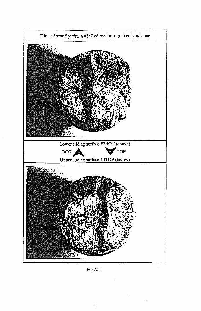
Direct Shear Specimen #3: Red medium-grained sandstone

Upper sliding surface #3T0P (below)

Fig. ALI

i

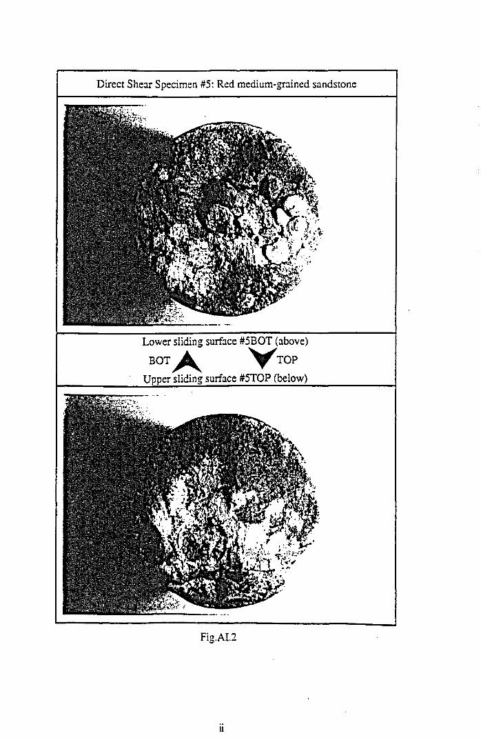
Direct Shear Specimen #5: Red medium-grained sandstone

Fig.AI.2

n

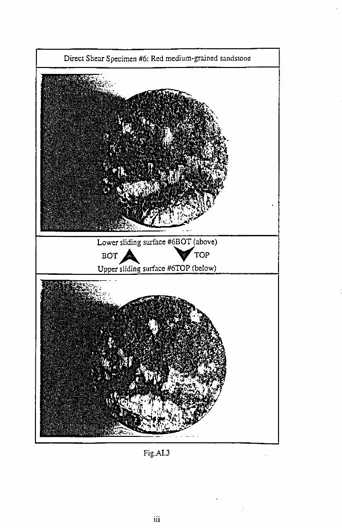
Direct Shear Specimen #6: Red medium-grained sandstone

Lower sliding surface #6BOT (above)

B O T ^ ^ TOP

Upper sliding surface #6TOP (below)

Fig.AI.3

in

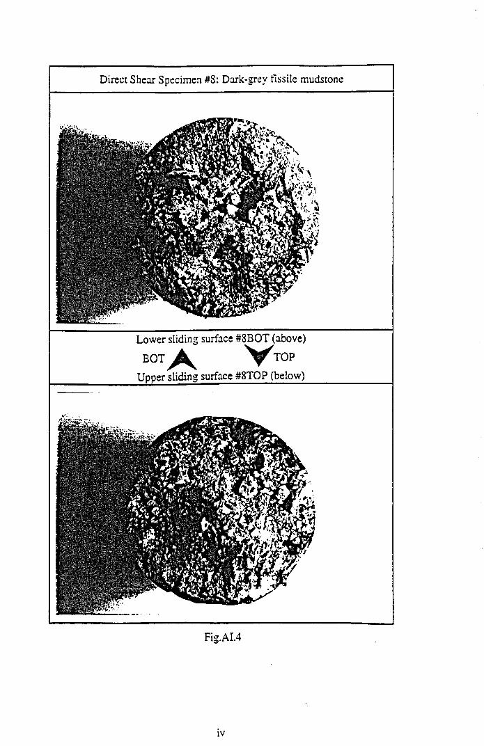
Direct Shear Specimen #8: Dark-grey fissile mudstone

Fig.AI.4

I V

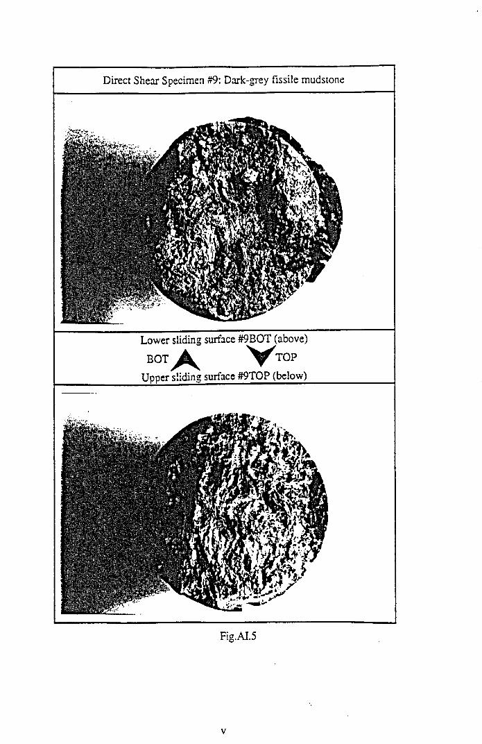
Direct Shear Specimen #9: Dark-grey fissile mudstone

Lower sliding surface #9BOT (above)

BOT ^ T O P

Upper sliding surface #9TOP (below)

■ f i

Fig.AI.5

v

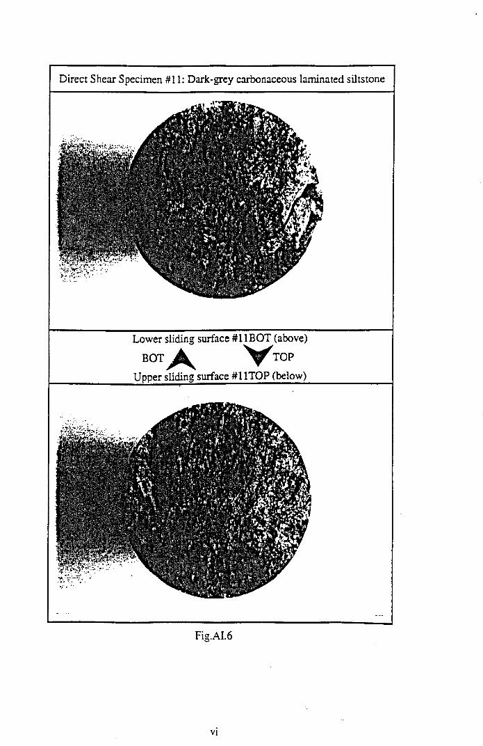
Direct Shear Specimen #11: Dark-grey carbonaceous laminated siltstone

Lower sliding surface #11B0T (above)

Fig.AI.6

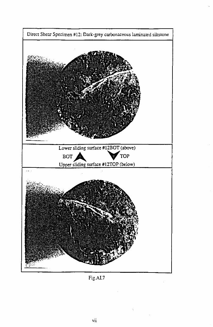
Direct Shear Specimen #12: Dark-grey carbonaceous laminated siltstone

Fig.AI.7

vu

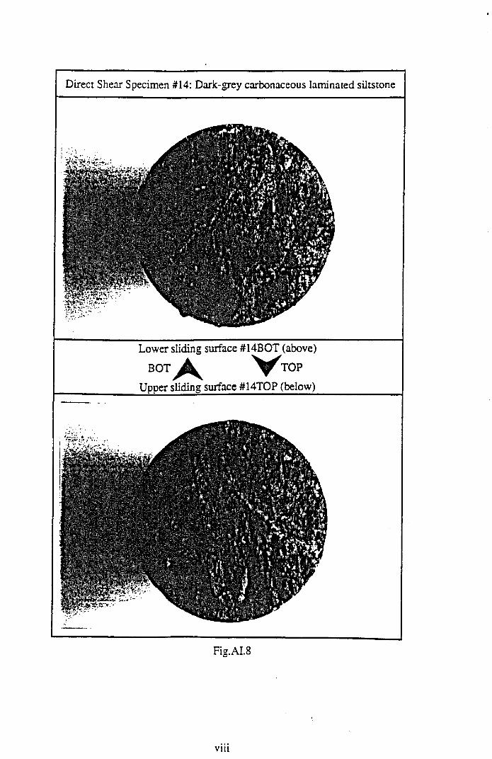
Direct Shear Specimen #14: Dark-grey carbonaceous laminated siltstone

Fig.AI.8

vm

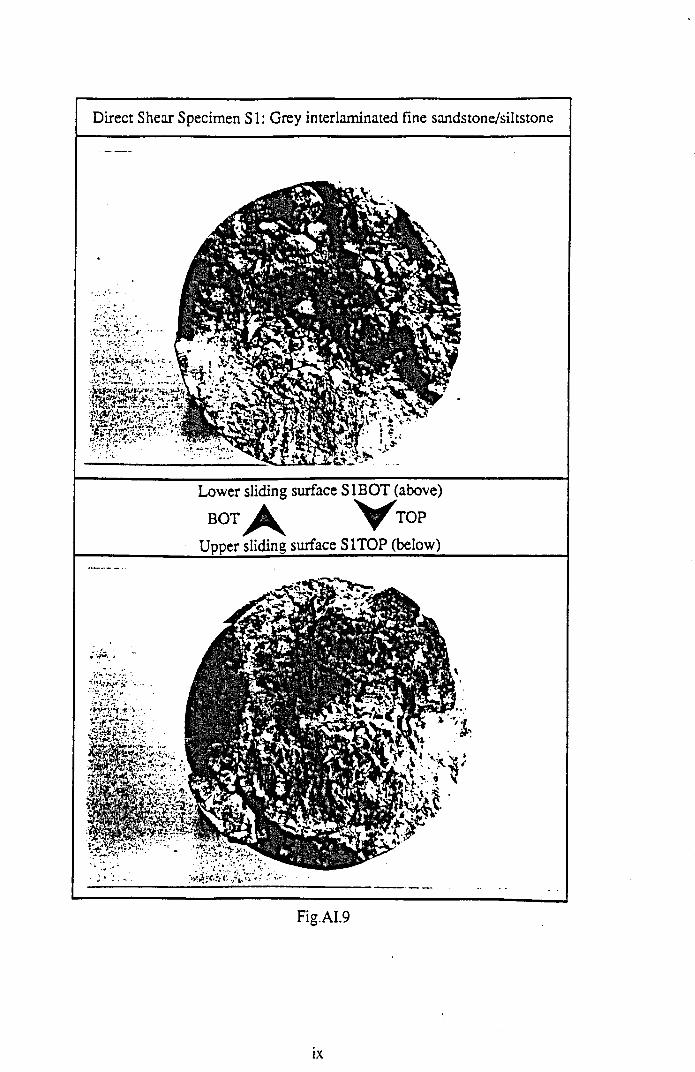
Direct Shear Specimen SI: Grey interlaminated fine sandstone/siltstone

Fig.AI.9

I X

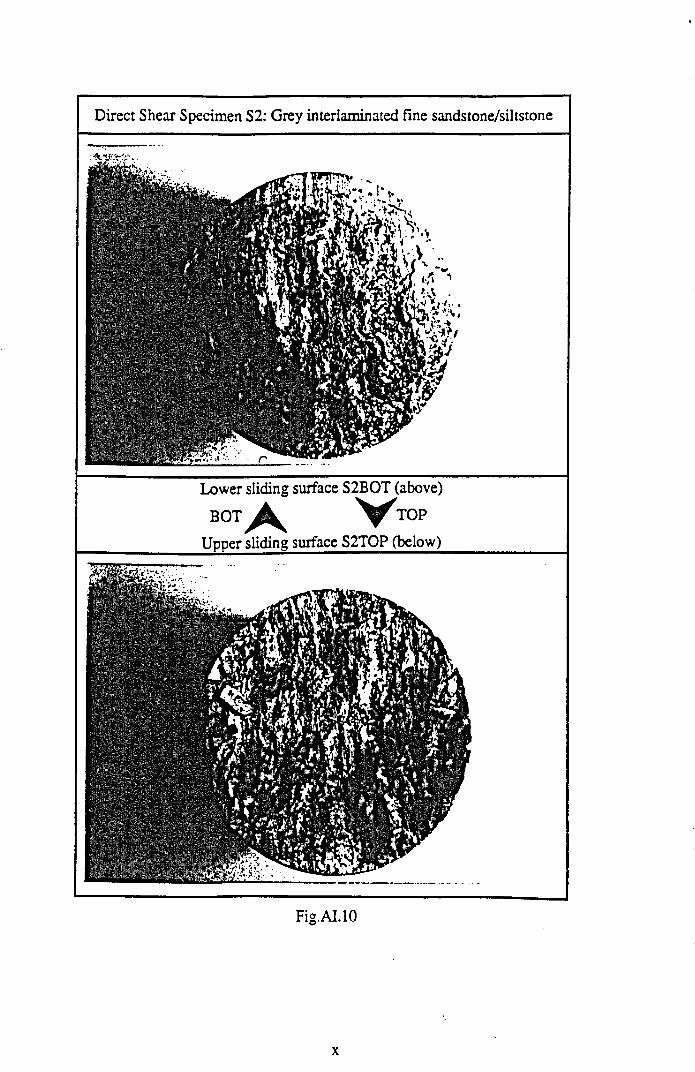
Direct Shear Specimen S2: Grey interlaminated fine sandstone/siltstone

Lower sliding surface S2BOT (above)

Fig. AI. 10

x

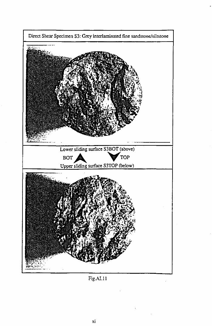
Direct Shear Specimen S3: Grey interlaminated fine sandstone/siltstone

Fig.ALll

xi

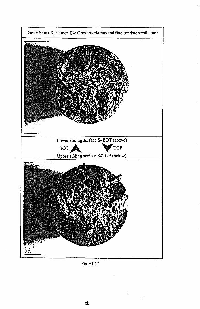
Direct Shear Specimen S4: Grey interlaminated fine sandstone/siltstone

Lower sliding surface S4BOT (above)

BOT A VtopUpper sliding surface S4TOP (below)

Fig.AI.12

xu

APPENDIX II

Clashach sandstone triaxial compression specimens #15 - #22:

• Fig.AII.l - AII.7: Temporal variation in differential stress, AE event rate, seismic b -value and inferred fractal dimension

• Fig.AII.8 - AII.14: Differential stress, AE event rate, seismic^ -value and inferred fractal dimension versus axial microstrain plots

383

Insta

i!Une

out S

dim

ic b

-val

ue

Diff

eren

tial S

ire.»

(MPa

)Qashach # IS: 1000|pti Hydrostatic to Dynamic Failure Claihadi #15: Frictional Sliding at lOOOpsi Confining Pressure

3S

Eid

Qashach #15: Frictional Sliding at 2000psi Confining Pressure

IIUÌ<

Fig. All. 1

Infe

rred

Frac

tal D

imen

sion,

D

AE

Even

t Ral

e (hi

ts/se

c)

Insta

ntan

eous

Sei

smic

b-v

alue

ts:

co•1II

Clashach <16: SOOQpsi Hydrostatic to Dynamic Failure

?

s2e>u

ID<

ag

Clashach <16: Frictional Sliding at SOOOpsi Confining Pressure

aIas2B>

Q£

CO

3§o§

•a1Ug

i§wA

Clashach <16: Frictional Sliding al 6000psi Confining Pressure

Fig.AII.2

Infe

rred

Frac

tal D

imen

sion,

D

AE

Even

t Rat

e (h

ils/se

c)

Insta

ntan

eous

Sei

smic

b-v

alue

CUshach (1 8 :7000psi Hydrosutic to Dynamic Failure Clashad) #18: Frictional Sliding at 8000psi Confining Pressure

1.5-1

1.0

0 5

I I I L

[-3 1 5 -

Q §

i I| a

-3 1.5-

o

3 !1 i

| ---

--1--

--a

ro

Infe

rred

Fra

cul D

u

Inst

anta

neou

s Se

isi

©

^6i

o1

. a

___

.___

__a_

____

1___

_

•2 « | , 0 -

V §1 sU MS -5

-1 0.5 - > 1 » »""1 1 ■ 8 T - I 1 1----200 400 600 800 1000 1200

Time (seconds)100 2 0 0

Tone (seconds)300 400 100 200

Time (seconds)

r 3

-2

300

Fig.All.3

Infe

rred

Frac

tal D

imen

sion,

D

AE

Even

t Ral

e (h

ils/se

c)

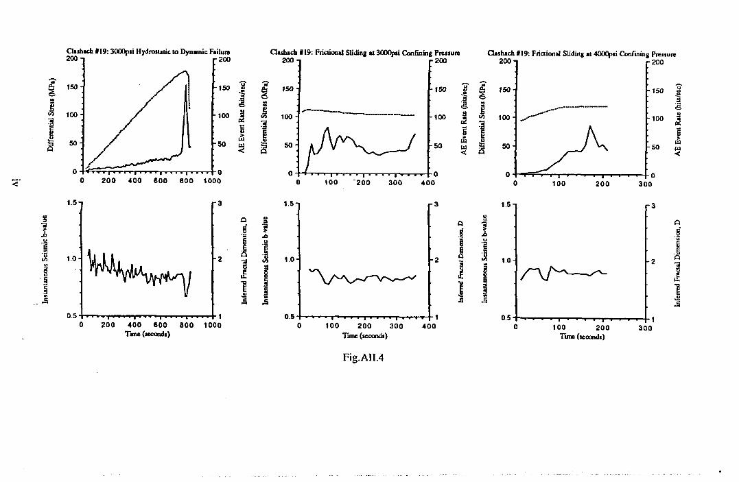
Insta

ntan

eous

Sei

smic

b-v

ilue

<

QJ

eu ,

1I

Ûi

aI

&

Fig.AII.4

Infe

rred

Frac

tal D

imen

sion,

D

AE

Even

t Rat

e (h

ils/se

c)

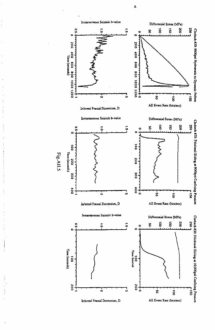
200 400

600 800

1000 1200 0

100 200

300 400

0 100

200Tim

e (seconds) Tim

e (seconds) Tim

e (seconds)

A

Instantaneous Seismic b-value

oÜI

Inferred Fractal Dimension, D

Instantaneous Seismic b-value

oin

Inferred Fractal Dimension, D

Instantaneous Seismic b-value

Differential Stress (MPa)

8 I 8 1

AE Event Rate (hits/sec)

Differential Stress (MPa)

8 8 8 1

AE Event Rate (hits/sec)

Differential Stress (MPa)

Inferred Fractal Dimension, D AE Event Rate (hits/sec)

Clashach #20: 9000psi Hydrostatic to D

ynamic Failure

Clashadi #20: Frictional Sliding at 9000psi Confining Pressure

Clashach #20: Frictional Sliding at 10,000psi Confining Pressure2

50

1

r 150

250 -j r

150 250 n

r

150

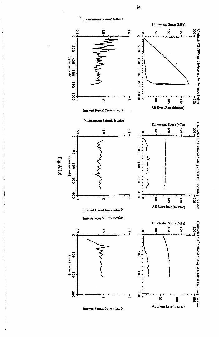
u

Instantaneous Seismic b-value

o — —6i o in

Inferred Fractal Dimension, D

Differentia] Stress (MPa)

AE Event Rate (hits/sec)

Instantaneous Seismic b-value

Inferred Fractal Dimension, D

Instantaneous Seismic b-value

Inferred Fractal Dimension, D

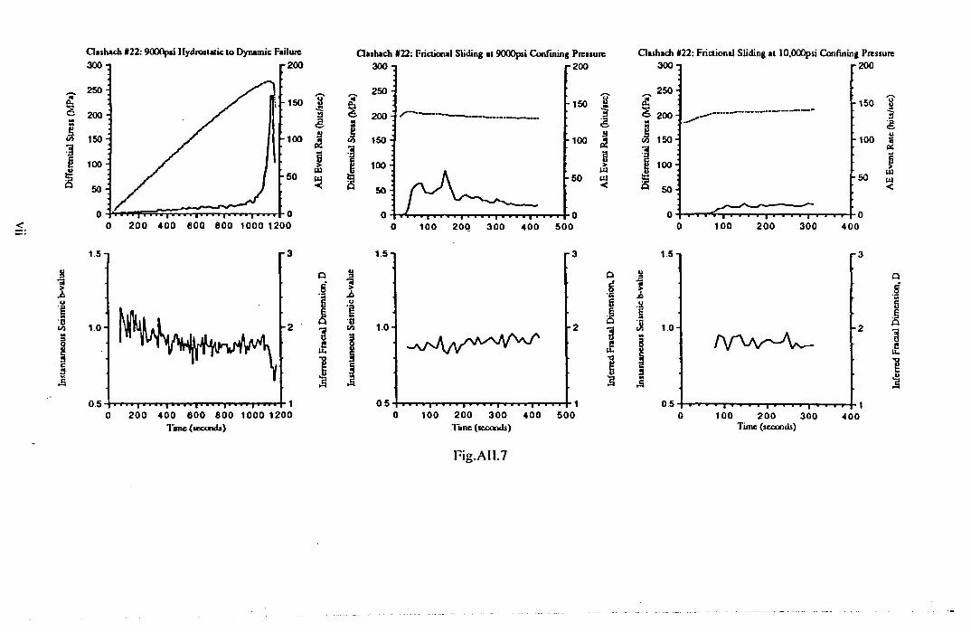
Insta

ntan

eous

Sei

smic

b-v

alue

CUshach #22: 9000p«i Hydrostatic to Dynamic Failure

lo n e (seconds)

£1%

CUshach #22: Frictional Sliding at 9000psi Confining Pressure Clashach #22: Frictional Sliding at lO.OOOpsi Confining Pressure

3■31u■gM0(A

5IMA

1.5 T

Qia6

1eu .

!200 300 400

Time (seconds)

3S

wId<

Fig.AII.7

Infe

rred

Frac

tal D

imen

sion,

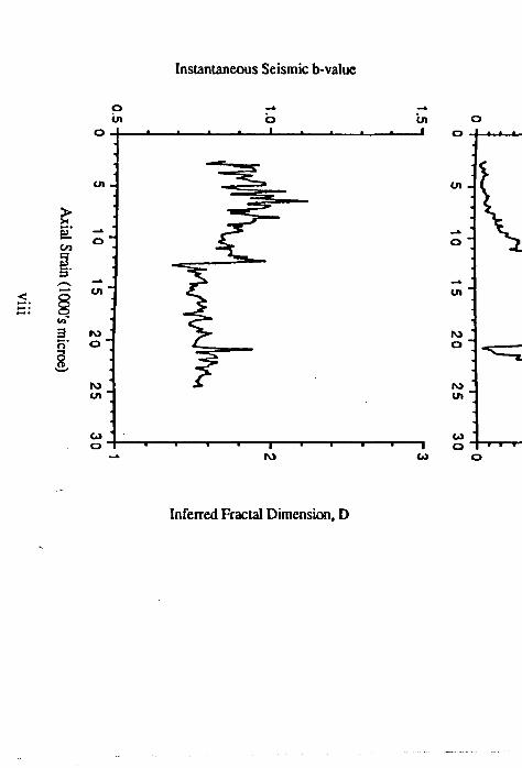
Axial Strain (1000's m

icroe)

Instantaneous Seismic b-value

oO) O Ul

o

OI

o

O I

ÍOO

loO I

oo

Inferred Fractal Dimension, D

o■ i i . « „ i

■ I « i io

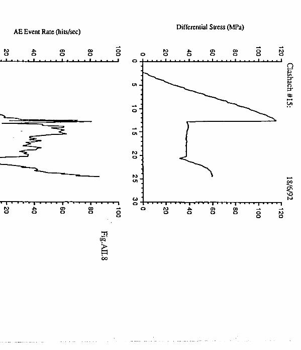
AE Event Rate (hits/sec)Differential Stress (MPa)

Ü1iÍq’

goo

Clashach #15:

18/6/92

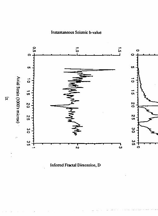
Axial Strain (1000's microe)

Instantaneous Seismic b-value

pin o

- i -in

^___ I

tn

m

roo

rocn

coo

U1

cn

roo

rocn

coo

COcn " 7 "ro

ico

cocn

01 — *- » ■

■ t ■ i i i

o

Inferred Fractal Dimension, D

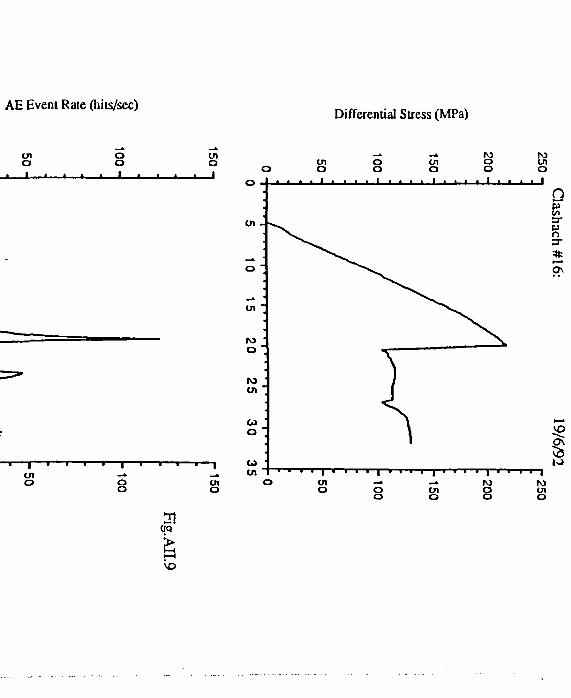
AE Event Rate (hits/sec)Differential Stress (MPa)

Ü!o q ’

èVO

Clashach#16:

19/6/92

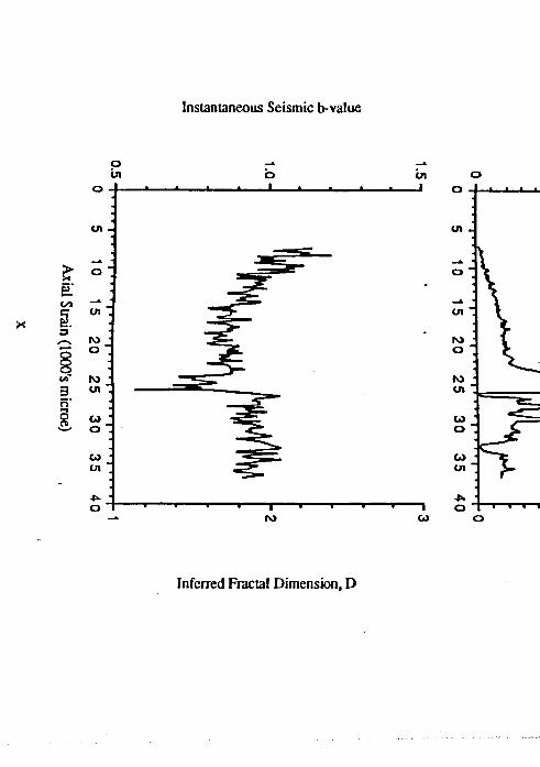
Axial Strain (1000’s microe)

Instantaneous Seismic b-value

o -*•in o in

o

roo

fOcn

coo

cocn

o

o- I * ‘ » ‘

11 ■ I I Io

Inferred Fractal Dimension, D

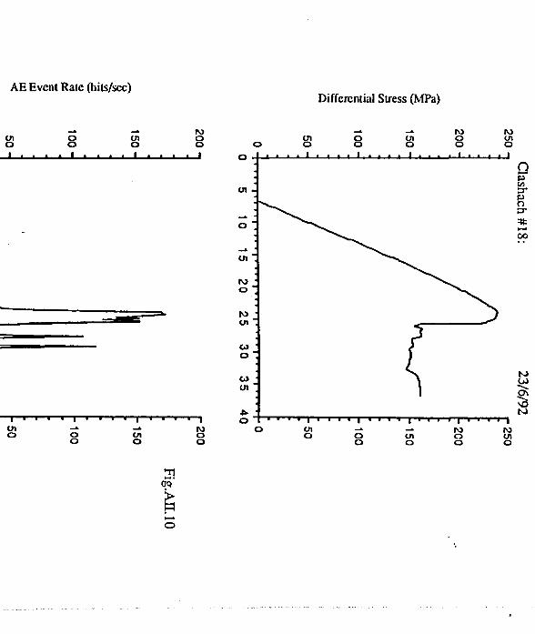
AE Event Rate (hits/scc)Differential Stress (MPa)

o

Clashach #18:

23/6/92

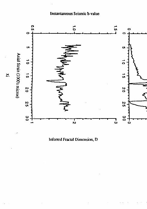
Axial Strain (1000’s m

icroe)

Instantaneous Seismic b-value

Inferred Fractal Dimension, D

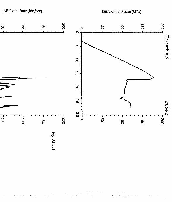
AE Event Rate (hils/sec) Differential Stress (MPa)

Clashach #19:

24/6/92

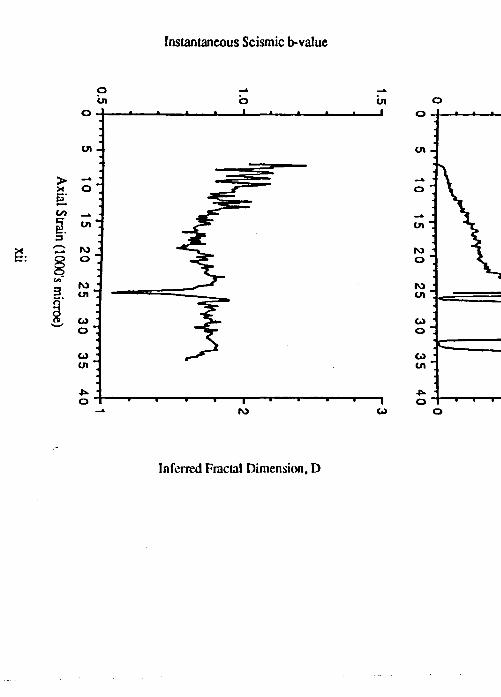
Axial Strain (1000's m

icroe)

Instantaneous Seismic b-value

Inferred Fractal Dimension, D

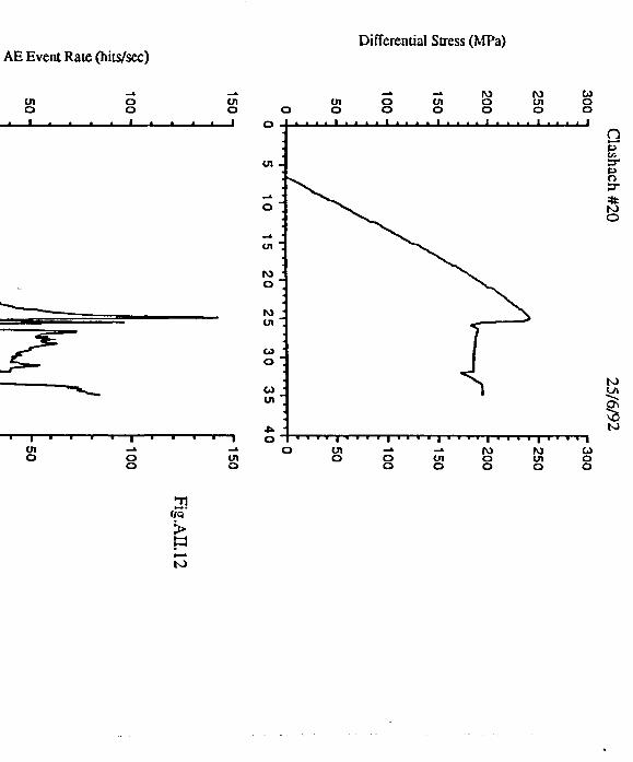
AE Event Rate (hits/sec)Differential Stress (MPa)

Clashach #20

25/6/92

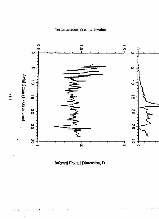
Axial Strain (1000's microe)

Instantaneous Seismic b-value

p -*In o In o

Inferred Fractal Dimension, D

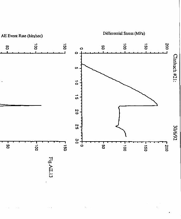
Clashac h #21: 30/6/92