Embed Size (px)
Citation preview
ELSEVIER Computer Physics Communications 120 (1999) 255-268
Computer Physics Communications
www.elsevier.nl/locate/cpc
An high performance Fortran implementation of a Tight-Binding Molecular Dynamics simulation
B. Di Martino a'1'4, M. Celino b'2, V. Rosato b,3 a Dipartimento di lngegneria dell'Informazione, Second University of Naples, Naples, Italy
b ENEA, HPCN Project, C.R. Casaccia, CP 2400, 00100 Rome AD, Italy
Received 30 July 1998; revised 10 February 1999
Abstract
Molecular Dynamics simulations in the Tight-Binding approach allow the study of the ionic and electronic structures of semiconductors. The Tight-Binding codes are characterized by inhomogeneous data distribution and requi,re the repeated diagonalization of a large sparse matrix to compute the whole body of its eigenvalues and eigenvectors. We describe the porting of this code on a parallel computer: we show the parallelization strategy for both the Molecular Dynamics part of the code and for the diagonalization needed at each time step. The parallelization has been carried out within the High Performance Fortran (HPF) environment, and tested on IBM SP architectures. The integration of optimized parallel mathematical routines is also described. © 1999 Elsevier Science B.V. All rights reserved.
PACS: 31.15.Q; 61.20.Ja; 07.05.B Keywords: Molecular Dynamics; Tight-Binding; Parallelization; Performances; HPF; Mathematical libraries; PESSL
PROGRAM SUMMARY Computers: IBM SP
Title of program: mdprs
Catalogue identifier: ADKP
Program Summary URL: http://www.cpc.cs.qub.ac.uk/cpc/summaries/ADKP
Program obtainable from: CPC Program Library, Queen's Uni- versity of Belfast, N. Ireland
Operating systems under which the program has been tested: UNIX-AIX
Programming language used: HPF and IBM-PESSL mathematical library
No. of bytes in distributed program, including test data, etc.: 39072
Distribution format: uuencoded compressed tar file
I E-mall: [email protected] 2 E-mail: [email protected] 3 E-mall: [email protected] 4 Corresponding author: Dipartimento di Ingegneria dell' Informazione, Facolth di Ingegneria, Second University of Naples, via Roma,
29-81031 Aversa (CE), Italy.
0010-4655/99/$ - see front matter © 1999 Elsevier Science B.V. All rights reserved. PII S0010-4655 (99 )0025 1-9
256 B. Di Martino et al./Computer Physics Communications 120 (1999) 255-268
Keywords: Molecular Dynamics, Tight-Binding, high performance Fortran, parallel, mathematical library
Nature of physical problem The parallel code simulates, using the Tight-Binding Molecular Dynamics technique, the atomistic evolution of semiconductor materials in several thermodynamic environments.
Method of solution The inter-atomic forces are derived by the Tight-Binding theory of electrons in solids. The atomic equations of motion are integrated by using the VI order Gear algorithm; the constant pressure- constant temperature ensemble is obtained by implementing the Parrinello-Rahman-Nos6 algorithm.
L O N G WRITE-U P
I. Introduction
Computer simulations at the atomic scale are among the most powerful theoretical tools used to investigate the properties of matter, from complex molecules to semiconductors. Materials Science has largely benefited of the enormous progress achieved in the last twenty years in this area which has let available a large set of models based on classical [ 1 ] up to fully ab initio or quantum mechanical [2] representations. It is now possible to select the computational model which offers the best compromise between the accuracy of the involved physical representation and the resulting computational cost. The Tight Binding (TB) model [3,4] has recently called the attention as being able to perform simulations of semiconductor materials combining high accuracy and a lower computational cost with respect to fully quantum mechanical (ab initio) schemes.
Although being much simpler than ab initio approaches, the computational complexity of TB algorithms is still considerable when used in combination to a Molecular Dynamics (MD) technique (TBMD) because it requires the repeated diagonalization of a large and sparse matrix. It is well known that the computational complexity of the matrix diagonalization scales with N 3 (O(N3)) , where N is the number of atoms of the system. As a consequence, the practical size of the simulated systems cannot exceed the limit of N = 300-400 atoms on a powerful workstation. Although several linearly scaling ( O ( N ) ) TB schemes have been developed (see for example [ 5 ] ), their use is not widely diffused, as they do not allow the evaluation of the electronic structure of the solid. Further difficulties in the use of the O ( N 3) approach arise with the memory occupancy as the size of the matrix involved in TB calculations is of the order k N x k N (with k -~ 10). While such a figure already allows the study of a number of relevant problems in the physics of semiconductors, it still leaves a large gap towards the true domain of Materials Science simulations which should be able to reproduce the macroscopic effects induced by objects (for example: grain boundaries, dislocations, interfaces, nanostructures, etc.) whose modelling requires a large number of atoms.
This limit can be overcome by porting the TBMD code on parallel computers. The aim of the present study is to realize a TBMD code which allows the study of systems constituted by a number of atoms of about 103 in the O ( N 3) formulation. In this work we report the parallelization of a O ( N 3) TBMD code, performed on a distributed memory MIMD computer (IBM SP), by using HPF (High Performance Fortran) and a set of mathematical libraries, contained in the package PESSL (Parallel Engineering and Scientific Subroutine Libraries), suitably parallelized to fit the architectural features of that computer.
The paper proceeds as follows: in the next section, the TB mathematical formalism is introduced; Section 3 is devoted to the introduction and description of the HPF language and the PESSL mathematical libraries; Section 4 is devoted to the analysis of the TBMD code from an algorithmic point of view and all the subroutines and main variables of the code are described; Section 5 shows how to run the code; Section 6 describes the main issues involved in the parallelization and in the strategy adopted; the last section, Section 7, discusses the code performances on several parallel computers of the IBM SP series.
B. Di Martino et al. / Computer Physics Communications 120 (1999) 255-268
2. The TB mathemat ical formalism
257
The goal of a generic MD code is to generate time trajectories of a system constituted by N atoms by solving the equations of motion depending on the forces acting on each atom. The forces can be calculated in a classical or in a quantum mechanics representation and they are the main computational task in both cases. Whereas in the classical representation force evaluation is essentially related to the calculation of the interparticle distances, in the TB representation there is a further computational complexity given by the diagonalization of the TB matrix (whose construction is related to the computation of the interparticle distances). The computational cost is, then, O ( N 2) scaling, in the case of classical regime and O ( N 3) in the TB case.
The TB formulation is based on the adiabatic approximation of the Hamiltonian Htot of a system of atoms and electrons in a solid [ 3],
ntot : 7]," -t- Te q- Uee "]- Uei "[- Uii , ( 1 )
where T/and Te are the kinetic energy of atoms and electrons, Uee, Uei, Uii are the electron-electron, electron- atom and atom-atom interactions, respectively.
Referring to the theory of one electron moving in the presence of the average field due to the other valence electrons and atoms, the reduced one-electron Hamiltonian can be written as
h = Ze -t- Uee -}- Uei, (2)
giving the eigenvalues (energy levels) e, and the eigenfunctions Igt,), where n is the rank of the matrix h. In the TB scheme, the eigenfunctions are represented as linear combinations of atomic orbitals kbt,~/,
= ( 3 )
la
where l is the quantum number indexing the orbital and ~z labels the atom. The expansion coefficients c~'~ represent the occupancy of the lth orbital located on the ~th atom.
In the present TB scheme, the elements of the h matrix, <4,¢,~lh14,t~>, connecting a and/3 nearest neighbours atoms are represented by the product of two contributions,
<4,,,,,Ih14~t~> = al, l f ( r a # ) , (4)
where at, t are parameters fitted on ab initio or experimental results, and f ( r~a) is a scaling function dependent on the particle distance r,,a. As a further approximation, a minimal basis set, i.e. the minimal set of electronic orbitals for each atom is usually adopted: four basis functions (s, Px, Py, Pz) per atom are known to be sufficient for a satisfactory description of the valence bands in the case of elemental semiconductors (silicon and carbon). In order to obtain the eigenvalues (the single-particle energies) E, and the eigenvectors c~ it is necessary to solve the secular problem at each MD time step. This implies repeated diagonalization of the matrix h, which introduces the O ( N 3) scaling. The rank of the matrix is determined by n = N x k where N is the number of atoms in the simulated systems and k is the dimension of the basis set (k = 4 in the simplest case of elemental semiconductors). Once the eigenvalues and the eigenvectors are known, the attractive potential energy can be computed and summed to the repulsive part Urep derived from a many-body approach [6],
Etot = ~ enf(en, T) + Urep, (5) n
where Ur~p is of the form
Urep = Z ~ ( r a B ) . ( 6 )
a>B
258 B. Di Martino et al./Computer Physics Communications 120 (1999) 255-268
Urep takes also into account the overlap interaction originated by the non-orthogonality of the basis orbitals and the possible charge transfer.
The Hamiltonian of Eq. ( l ) refers only to the atomic coordinates describing the internal degrees of freedom of the system. In order to simulate the interaction with the surrounding, suitable MD schemes have been devised to account for a coupling between the internal degrees and the external degrees of freedom (thermal bath and possibility of imposing to the system an external stress). Introducing further degrees of freedom simulates the coupling. The MD simulation in the isothermal-isobaric ensemble requires the presence of l0 extra variables which are coupled to the internal degrees of freedom via suitable parameters which can be adjusted to ensure the fastest convergence to equilibrium (Parrinello-Rahman and Nos6 algorithm [ 7 ] ).
After the calculation of the force on each atom, the equations of motion can be integrated by using a finite difference scheme. In this code, a sixth-order predictor-corrector scheme (VI order Gear algorithm) [8] has been implemented in view of its good accuracy.
3. HPF and PESSL
To reach the target of the full parallelization of the TBMD code, we have chosen the approach of utilization of very high level frameworks: HPF parallel language and PESSL mathematical library.
High Performance Fortran (HPF) [9,10] is a high level language that simplifies the programming and the porting of codes on distributed or shared memory parallel computers.
Essentially HPF provides a standardized set of extensions to Fortran 90 and Fortran directives to enable the execution of a sequential program on parallel computer systems. Its main feature is to eliminates the complex, error prone task of explicitly programming how, where and when to pass messages between processors on distributed memory machines.
The most popular programming model for massively parallel computers is the Single Program Multiple Data (SPMD) [1 1] model: the same program, not necessarily the same instruction stream, is executed by each processor, each operating on a part of the data. Given the data-distribution, an HPF compiler automatically transforms intrinsically data-parallel applications, written in the standard sequential Fortran 90 language, into SPMD message-passing programs by partitioning and distributing its data as specified by directives. Furthermore, it allocates the computations to processors according to the locality of the data references involved, and it inserts any necessary data communications in an implementation-dependent manner, e.g. by message passing or by a shared memory mechanisms. Compiler directives such as PROCESSORS, ALIGN, DISTRIBUTE and TEMPLATE are introduced to control the alignment and distribution of array elements on the (abstract) processors; directives such as INDEPENDENT and language constructs such as FORALL are introduced to express data parallelism.
The performance of a SPMD program depends critically on its data mapping. HPF allows for testing the efficiency attained with different data mappings by simply changing the directives in the program instead of recoding a message-passing program. The writing of efficient HPF programs is not, however, a trivial task. Indeed, the high-level nature of the language prevents the user from clearly understanding the behaviour of the parallel code being produced by the compiler, and that can frequently lead to inefficient codes. Apparently simple operations can be translated into a code involving enormous amounts of communication. Anyway, HPF is broadly recognized as being the tool of choice for porting big legacy sequential codes to parallel architectures, when the computation exhibits regular data-parallel behaviour, and it can be effective even when the computation presents characteristics of irregularity (see, e.g., [ 12] ).
The second step is the choice of the mathematical library to integrate within the parallel TBMD. We have chosen a library that can perform the matrix diagonalization and that can be used jointly with the HPF directives: the Parallel ESSL [ 14].
The Parallel ESSL is a parallel mathematical library specifically tuned for the IBM SP computers and can be called both from message passing routines and HPF framework. In the latter case the efficiency of the matrix
B. Di Martino et al./Computer Physics Communications 120 (1999) 255-268 259
distribution and of the startup of the diagonalization are lower than in the message passing framework, but the implementation is simpler. This allows a sharp tuning of the parameters needed for the parai~ei routine.
The linear algebra section of the PESSL is based on the ScaLAPACK [ 13] public domain software. Also in this case, PESSL assumes that the application program is using the SPMD programming model ]Zor commu- nicafton, PESSL includes the Basic Linear A~gebra Communications Subprograms {BLACS), which use the Para[[e[ Environment (PE) and the Message Passing Interface (MPD communication [ibrary~
4. The program structure
4.1. Scheme o f the TBMD computation
The layout of the generic iteration step of the sequential TBMD code consists in the following steps: (1) Predictor part of the integration of the dynamical equations for the evolution of the 3N 4- 10 degrees of
freedom. (2) Computation of the interparticle distances r,,~: this is used to fill the matrix of nearest neighbours and
the array to store the number of nearest neighbours of each atom. (3) Computation of the matrix elements (4't,~,lh[4~t~). (4) Diagonalization of the real skew matrix h for the computation of the half spectrum of eigenvectors and
eigenvalues. This is the most computational intensive part of the code; every tphys time steps the whole spectrum of eigenvectors and eigenvalues must be computed for post processing study of the electronic properties of the material.
(5) Computation of the attractive part of the atomic forces (Feynman routine): the attractive part of the forces acting on each atom are computed using both the eigenvalues and the eigenvectors computed in the previous step.
(6) Computation of the repulsive part of the atomic forces: this part of the forces depends only by the distances among the atoms: the nearest neighbours matrix is thus used.
(7) Corrector part of the integration of the dynamical equations for the evolution of the 3N 4- 10 degrees of freedom.
(8) All the physical quantities are evaluated and every tphys time steps the values are stored on disk. The predictor-corrector scheme requires the knowledge of the atomic coordinates till the fifth order derivative:
the whole atomic system is thus described by 3 × 6 arrays of length N for the coordinates and by further 6 arrays of the same length to store the forces (3 for the attractive part and 3 for the repulsive part). A N x N matrix is requested to store the interparticle distances. For minimizing the computation of the TB h matrix, the components of the forces and of the distances are also stored in 9 arrays of dimension N. The h matrix of dimensions at least 4N × 4N must be allocated.
The main difficulties in the parallelization of a TBMD code are: • the system cannot be mapped on a regular grid (atoms can move inside the simulation box); • diagonalization of a large sparse matrix is involved (parallel math libraries for sparse-matrix diagonalization
are not yet available).
4.2. Program files
The code is composed by the following files: • The main program and 14 subroutines in the file: mdprs.f. • 19 include files: acc.inc, dist.inc, eigen.inc, erg.iuc, fhf.inc, frep.iue, ftot.inc, func.inc, include.inc, latt.inc,
lst.inc, param.inc, pos.inc, potz.inc, simul.inc, tb.inc, vel.inc. • 1 input file: data.inc.
260 B. Di Martino et al./Computer Physics Communications 120 (1999) 255-268
• 1 command file for job submission: run.cmd. • 1 makefile.
The main program performs the following operations: it reads the input data; it initializes the starting configuration and all the variables; it controls the MD loop aver the selected number of time steps. In the main program also all the physical quantities and the new coordinates are calculated and recorded on disk.
The 14 subroutines are the following: ( 1 ) ch_timestep: It performs the rescaling of the dynamical variables when a new run, restarting run from a
previous one, is performed with a different time step. (2) crystal: It defines the tight-binding, repulsive potential and lattice parameters. (3) feynman: It computes the Hellmann-Feynman forces and the attractive part of the virial. (4) fifth_ord_cor: It performs the corrector phase of the predictor-corrector algorithm for the integration of
the equations of motions. (5) fifth_ord_pred: It performs the predictor phase of the predictor-corrector algorithm for the integration of
the equations of motions. (6) forze: In this subroutine is collected all the instructions for the calculations of the forces acting on the
atoms in the system. This subroutine calls the htb, feynman, repuls subroutines. (7) h_evol: It calculates all the quantities related the simulation box: the volume, the deformations, the internal
angles. (8) htb: It computes the starting atomic configuration, in the diamond structure, when the ICON variable
is set to 0. This is useful when a simulation for silicon or carbon at room temperature is needed (for example).
(9) h_pred: It calculates the predictor phase of the predictor-corrector algorithm for the solution of the differential equations describing the deformations of the simulation box.
(10) repuls: It computes the repulsive energy and the repulsive contribution to the forces acting on the atoms. ( 11 ) scale_vel: It gives the initial velocities of the atoms in the simulation box. (12) syevx_shield: It calls the PESSL mathematical routine for the calculation of the eigenvalues and eigen-
vectors of the tight-binding matrix. This calculation is performed in parallel. (13) virein_sum: It calculates the kinetic energy of the system and the kinetic part of the virial.
Finally, the function randy for the generation of random numbers in the interval ]0,1[ is called by the subroutine scale_vel for assigning the velocities to the atoms accordingly to the selected temperature.
4.3. Program variables
In this section the main variables are listed. All the others are referenced in the main program and in the subroutines.
4.3.1. The input file data.inc First of all, some variables must be initialized using the file data.inc; using these variables the type and the
length of the simulation can be chosen:
natom: number of atoms;
namax: maximum number of atoms;
temp: selected temperature;
kwrite: frequency of output of the physical quantities on the standard output;
maxstp: maximum number of time steps;
icon: if icon = 0 the starting configuration is calculated by the program in diamond-like configuration, if icon = - 1 restart from unformatted file of a revious run, if icon= 1 restart from formatted file of a revious run;
B. Di Martino et al./Computer Physics Communications 120 (1999) 255-268
step: time step;
istep: if istep= 1, the time step is changed;
step2: new time step;
pwant: selected external pressure;
pminv: mass of the piston (Parrinello-Rahman algorithm) that controls the internal pressure;
ssss: mass of the piston (Nos6 algorithm) that controls the internal temperature;
kstoc: frequency of saving in a file all the informations needed for the restart the restart;
kconf: frequency of saving the atomic coordinates in a file for postprocessing purposes;
iscri: output logical unit for writing the physical quantities;
cut: cutoff of the interatomic potential;
lO: length of the unitary cell in the diamond structure.
261
4.3.2. Other important variables in the code In the code the main variables are:
x y z: atomic coordinates (vectors of length namax);
hp: matrix describing the simulation cell (3 × 3 array);
h: matrix describing the electronic contribution in the attractive part of the forces. This matrix must be diagonalized at each time step;
fx fy fz: forces acting on each atom (vectors of length namax);
aca: array where the physical quantities are saved and averaged;
etotal: total energy of the system;
ekin: kinetic energy;
nstep: number of time steps calculated during the MD run;
tmp: instantaneous temperature.
5. The job setup
5.1. Preparing the input data
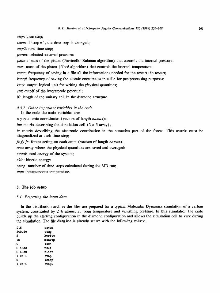
In the distribution archive the files are prepared for a typical Molecular Dynamics simulation of a carbon system, constituted by 216 atoms, at room temperature and vanishing pressure. In this simulation the code builds up the starting configuration in the diamond configuration and allows the simulation cell to vary during the simulation. The file data.ine is already set up with the following values:
216 natom
300.dO temp
5 kwrite
10 maxstp
0 icon
6.46d0 rcut
6.66d0 rlist 1.0d-I step
0 istep
1.0d-1 step2
262 B. Di Martino et al./Computer Physics Communications 120 (1999) 255-268
O.dO pwant
50000.dO pminv
200.dO ssss
1 kstoc
I kconf
5 iscri
2 . 6 c u t
3 . 5 4 8 10
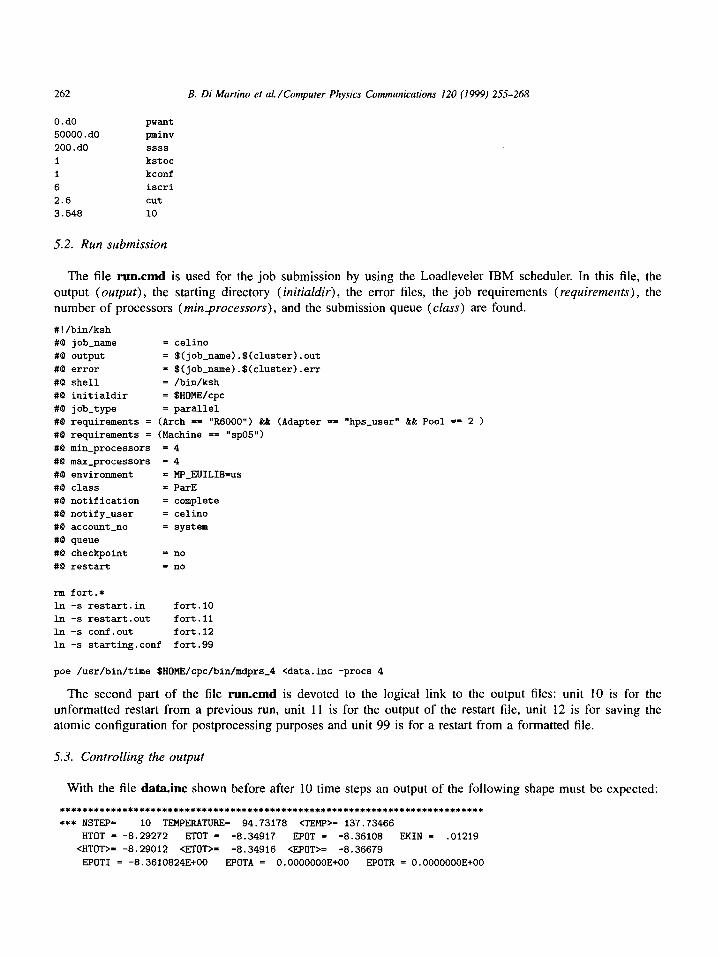
5.2. Run submission
The file run.cmd is used for the job submission by using the Loadleveler IBM scheduler. In this file, the output (output), the starting directory (initialdir), the error files, the job requirements (requirements), the number of processors (rain_processors), and the submission queue (class) are found.
#!/bin/ksh
#@ job_name = celino
#@ output = $(job_name).$(cluster).out
#@ error = $(job_name).$(cluster).err
#© shell = /bin/ksh
#@ initialdir = $HOME/cpc
#@ job_type = parallel
#@ requirements = (Arch == "R6000") &~ (Adapter == "hps_user" aa Pool == 2 )
#@ requirements = (Machine == "sp05")
#@ min_processors = 4
#@ max_processors
#@ environment
#@ class
#@ notification
#@ notify_user
#@ account_no
#© queue
#© checkpoint
#~ r e s t a r t
=4
= MP_EUILIB--us
= Pare
= complete
= celino
= system
= no
= no
rm fort.*
in -s restart.in fort.lO
in -s restart.out forZ.11
in -s conf.out fort.12
in -s starting.conf fort.99
poe /usr/bin/time SHOME/cpc/bin/mdprs_4 <data.inc -procs 4
The second part of the file run.cmd is devoted to the logical link to the output files: unit 10 is for the unformatted restart from a previous run, unit II is for the output of the restart file, unit 12 is for saving the atomic configuration for postprocessing purposes and unit 99 is for a restart from a formatted file.
5.3. Controlling the output
With the file data.inc shown before after 10 time steps an output of the following shape must be expected:
*** NSTEP= 10 TEMPERATURE= 9 4 . 7 3 1 7 8 <TEMP> = 1 3 7 . 7 3 4 6 6
HTOT = -8.29272 ETOT = -8.34917 EPOT = -8.36108 EKIN = .01219
<HTOT>= -8.29012 <ETOT>= -8.34916 <EPOT>= -8.36679
EPOTI = -8.3610824E+00 EPOTA = O.O000000E+O0 EPOTR = O.O000000E+O0
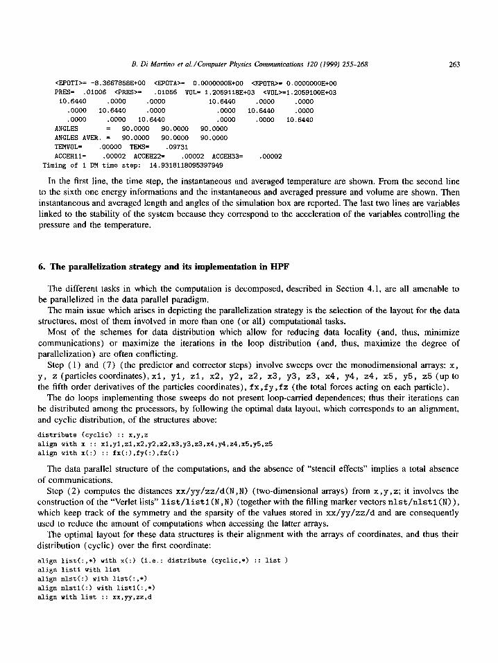
B. Di Martino et al./ Computer Physics Communications 120 (1999) 255-268 263
<EPOTI>= -8.3667858E+00 <EPOTA>= 0.0000000E+00 <EPOTR>= 0.0000000E+00 PRES= .01006 <PKES>= .01056 VOL= 1.2059118E+03 <VOL>=1.2059100E+03
10. 6440 .0000 .0000 10. 6440 .0000 .0000
.0000 i0. 6440 .0000 .0000 10. 6440 .0000
.0000 .0000 10. 6440 .0000 .0000 10. 6440
ANGLES = 90. 0000 90. 0000 90. 0000
ANGLES AVER. = 90.0000 90.0000 90.0000
TEMVOL= .00000 TEMS= .09731
ACCEHII = .00002 ACCEH22= .00002 ACCEH33= .00002
Timing of 1 DM time step: 14.9318118095397949
In the first line, the time step, the instantaneous and averaged temperature are shown. From the second line to the sixth one energy informations and the instantaneous and averaged pressure and volume are shown. Then instantaneous and averaged length and angles of the simulation box are reported. The last two lines are variables linked to the stability of the system because they correspond to the acceleration of the variables controlling the pressure and the temperature.
6. The parallelization strategy and its implementation in HPF
The different tasks in which the computation is decomposed, described in Section 4.1, are all amenable to be parallelized in the data parallel paradigm.
The main issue which arises in depicting the parallelization strategy is the selection of the layout for the data structures, most of them involved in more than one (or all) computational tasks.
Most of the schemes for data distribution which allow for reducing data locality (and, thus, minimize communications) or maximize the iterations in the loop distribution (and, thus, maximize the degree of parallelization) are often conflicting.
Step (1) and (7) (the predictor and corrector steps) involve sweeps over the monodimensional arrays: x , y , z (particles coordinates), x l , y l , z l , x2, y2, z2, x3, y3, z3, x4, y4, z4, x5, yS, z5 (up to the fifth order derivatives of the particles coordinates), f x , f y , f z (the total forces acting on each particle).
The do loops implementing those sweeps do not present loop-carried dependences; thus their iterations can be distributed among the processors, by following the optimal data layout, which corresponds to an alignment, and cyclic distribution, of the structures above:
distribute (cyclic) :: x,y,z
align with x :: xl,yl,zl,x2,y2,z2,x3,y3,z3,x4,y4,z4,x5,y5,z5
align with x(:) :: fx(:),fy(:),fz(:)
The data parallel structure of the computations, and the absence of "stencil effects" implies a total absence of communications.
Step (2) computes the distances xx/yy/zz/d(N,N) (two-dimensional arrays) from x , y , z ; it involves the construction of the "Verlet lists" l i s t / l i s t 1 (N,N) (together with the filling marker vectors n l s t / n l s t i (N)), which keep track of the symmetry and the sparsity of the values stored in x x / y y / z z / d and are consequently used to reduce the amount of computations when accessing the latter arrays.
The optimal layout for these data structures is their alignment with the arrays of coordinates, and thus their distribution (cyclic) over the first coordinate:
align list(:,*) with x(:) (i.e.: distribute (cyclic,*) :: list )
align list1 with list
align nlst(:) with list(:,*)
align nlstl(:) with listl(:,*)
align with list :: xx,yy,zz,d
264 B. Di Martino et al . / Computer Physics Communications 120 (1999) 255-268
j .................... ! ....................
4i ~ ................... ' ....................
J
h d
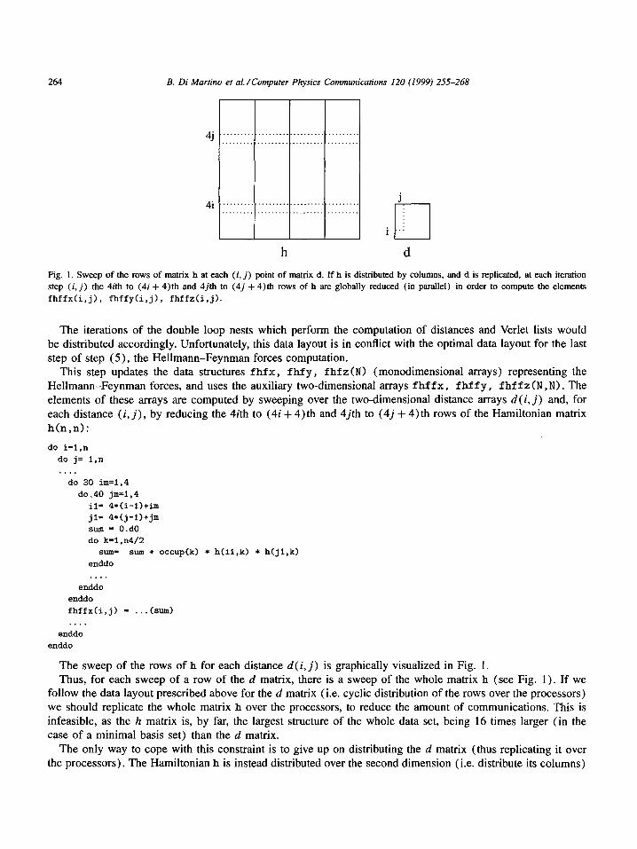
Fig. 1. Sweep of the rows of matrix h at each ( i , j ) point of matrix d. I f h is distributed by columns, and d is replicated, at each iteration step ( i , j ) the 4ith to (4i + 4)th and 4jth to (4j + 4)th rows of h are globally reduced (in parallel) in order to compute the elements fhffx(i,j), fhffy(i,j), fhffz(i,j).
The iterations of the double loop nests which perform the computation of distances and Verlet lists would be distributed accordingly. Unfortunately, this data layout is in conflict with the optimal data layout for the last step of step (5) , the Hellmann-Feynman forces computation.
This step updates the data structures f h f x , f h f y , f h f z ( N ) (monodimensional arrays) representing the Hellmann-Feynman forces, and uses the auxiliary two-dimensional arrays f h f f x , f h f f y , f h f f z ( N , N ) . The elements of these arrays are computed by sweeping over the two-dimensional distance arrays d(i , j ) and, for each distance (i , j) , by reducing the 4ith to (4i + 4)th and 4jth to (4j + 4)th rows of the Hamiltonian matrix h(n,n):
do i=l,n
do j= 1,n
do 30 im=l.4
do.40 jm=l,4
ii = 4. (i-1)+im j l = 4*(j-l)+jm sum = O.dO do k=l ,n4/2
sum= sum + occup(k) * h(il,k) * h(jl,k)
enddo
enddo
enddo
fhffx(i,j) = ...(sum)
enddo
enddo
The sweep of the rows of h for each distance d(i, j) is graphically visualized in Fig. 1. Thus, for each sweep of a row of the d matrix, there is a sweep of the whole matrix h (see Fig. 1). If we
follow the data layout prescribed above for the d matrix (i.e. cyclic distribution of the rows over the processors) we should replicate the whole matrix h over the processors, to reduce the amount of communications. This is infeasible, as the h matrix is, by far, the largest structure of the whole data set, being 16 times larger (in the case of a minimal basis set) than the d matrix.
The only way to cope with this constraint is to give up on distributing the d matrix (thus replicating it over the processors). The Hamiltonian h is instead distributed over the second dimension (i.e. distribute its columns)
B. Di Martino et al./Computer Physics Communications 120 (1999) 255-268
Table 1 Serial code performances on a single IBM SP thin node located at the ENEA, Frascati
265
Routine 216 atoms 512 atoms
Time (s) Rel. perc. (%) Time (s) Rel. pere. (%)
Whole code 40.2 - 386.1 TB matrix diagonalization 27.3 68 317.0 82 Feynman routine 8.4 21 64.1 17 Rest of the code 4.5 11 5.0 1
The time is expressed in seconds per time step. It is clear that the diagonalization routine is the most CPU-time consuming part of the code. Nevertheless, also the computation of the attractive forces (Feynman routine) must be parallelized to reach a good performance.
(see Fig. 1). The sweep over the elements of the d matrix is thus replicated, but the reduction of the 8 rows of h, for each distance ( i , j ) , can be performed in parallel: each processor sweeps the portion of rows of h assigned to it, and performs a partial reduction of those elements. The results of the partial reduction operated from each processor are then composed and the result of the final reduction is then broadcasted. The amount of distribution of the iterations of the overall loop nest (and thus the degree of parallelization) remains the same as in the case of the alternative data layout (distributed distances, and replicated Hamiltonian). With the latter scheme, there is an additional communication overhead due to the communication of the partial results of the reduction. This overhead, however, turns out to be negligible with respect to the computation overhead, and thus the efficiency is gained by the parallel execution.
Instead of redistributing the d matrix from the optimal data layout of step (2) to the whole replication needed in this step, we preferred to keep these matrices always replicated (thus also during step (2)) : even though the computation is in this way replicated among the processors during that phase, the communication overhead occurring during the redistribution of those matrices would be much more costly than the computation overhead of the replication of step (2).
In step (3) and (4) the computation and diagonalization of the Hamiltonian two-dimensional matrix h (n, n), and computation of its eigenvalues in the monodimensional array ova l (n) are performed. The PESSL routine SYEVX is called for this task. The parameters in the tuning process are those: (a) to control the absolute tolerance on the eigenvalues, which has been tuned to obtain the minimum of tolerance to improve the efficiency of the algorithm for the orthogonalization of the eigenvectors; (b) to balance the workspace and the memory requested for the eigenvectors calculations.
The use of the PESSL routine introduces extra inter-node communications because the SYEVX routine needs the matrix to be distributed in both dimensions as cyclic. We thus need to redistribute the Hamiltonian matrix h during this step, and to restore its distribution over the columns as needed in the Hellmann-Feynman routine.
7. Benchmarks of the parallel code and conclusions
To validate the porting and the data distribution adopted we have performed several runs on two IBM SP platforms: the first one is located at the ENEA Research Centre in Frascati (Italy) and the other at the IBM Centre of Poughkeepsie (USA). The first has 390-series processors with 66 MHz and 128 MB RAM, while the second has 397-series processors with 160 MHz and 256 MB RAM.
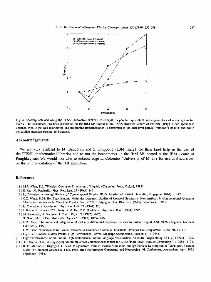
We have used the same test case for the benchmark of the sequential code. The runs have been performed on 2, 4, 6 and 8 processors. A clear speedup till 8 nodes is shown both using the SP at the ENEA Centre and the one at the IBM Centre (see Figs. 2 and 3). Furthermore, in Fig. 4 we report the speedup of the PESSL subroutine SYEVX used in the parallel code to compute half spectrum (eigenvalues and eigenvectors) of the
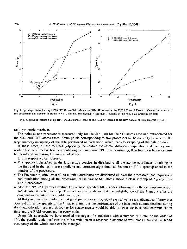
266 B. Di Martino et al./Computer Physics Communications 120 (1999) 255-268
3 ==
e~ 03
2
' i
~ 8 6 4 " 8 6 4 matrix (216 atoms) J
#
[3 - ' -E l 2048~2048 matrb( (512 atoms) J .
2 4
Processors
Fig. 2
/ C~E)2048 "2048 matrix (512 atoms)
I ~ i , i , i ,
2 4 6 8 Processors
Fig. 3
Fig. 2. Speedup obtained using HPF+PESSL parallel code on the IBM SP located at the ENEA Frascati Research Centre. In the case of two processors and number of atoms N = 512 and 640 the speedup is less than 1 because of the huge data swapping on disk.
Fig. 3. Speedup obtained using HPF+PESSL parallel code on the IBM SP located at the IBM Centre of Poughkeepsie (USA).
real symmetr ic matrix h. The point at one processor is measured only for the 216- and for the 512-atoms case and extrapolated for
the 640- and 1000-atoms cases. Some points corresponding to two processors lie below unity because of the large memory occupancy of the data partit ioned on each node, which leads to swapping of the data on disk.
In these cases, all the routines (especial ly the routine for atomic distance computation and the Feynman routine for the attractive force computat ion) become more CPU time consuming, therefore their behavior must be monitored increasing the number of atoms.
In this respect we can observe: • The approach described in the last section consists in distributing all the atomic coordinates obtaining in
the first and in the last phase (predictor and corrector algorithm, see Section (4 .1 ) ) a speedup equal to the number of the processors.
• The Feynman routine, even if the atomic coordinates are distributed all over the processors thus requiring a communicat ion among all the processors, in the case of 640 atoms, shows a clear speedup of 2 going from 4 to 8 processors.
• Also the SYEVX parallel routine has a good speedup till 8 nodes allowing its efficient implementation and its use at each time step. This fact indirectly shows that the redistribution of the h matrix after the diagonalizat ion takes a negligible wall-time. At this point we must underline that good performance is obtained even if we use a mathematical library that
does not utilize the sparsity of the h matrix to improve the performance of the inter-node communicat ions during the diagonal izat ion process. A routine for sparse matrix would be able to lower the inter-node communication time and the R A M occupancy on every node.
Using this approach, we have reached the target of simulations with a number of atoms of the order of 103: the parallel code performs the MD simulation in a reasonable amount of wall clock time and the RAM occupancy of the whole code can be managed.
B. Di Martino et al./Computer Physics Communications 120 (1999) 255-268
5 . , . J . , . / G--0864"864 matrix (216 atoms) / [3---D2048"2048 matrix (512 atoms) /
4
3
2
1
i i t
0 2 4 6 8
Processors
267
Fig. 4. Speedup obtained using the PESSL subroutine SYEVX to compute in parallel eigenvalues and eigenvectors of a real symmetric matrix. The benchmark has been performed on the IBM SP located at the ENEA Research Centre of Frascati (Italy). Good speedup is obtained even if the data distribution and the routine implementation is performed in the high level parallel framework of HPF and not in the explicit message passing environment.
Acknowledgements
We are very grateful to M, Briscolini and S. Filippone (IBM, Italy) for their kind help in the use of the PESSL mathematical libraries and to run the benchmarks un the IBM SP located at the IBM Centre of Poughkeepsie. We would like also to acknowledge L. Colombo (University of Milan) for useful discussions on the implementation of the TB algorithm.
References
[ I I M.P. Allen, D.J. Tildesley, Computer Simulation of Liquids (Clarendon Press, Oxford, 1987). 121 R. Car, M. Parrinello, Phys. Rev. Lett. 55 (1985) 2471. 131 L. Colombo, in: Annual Review of Computational Physics IV, D. Stauffer, ed. (Word Scientific, Singapore, 1996) p. 147. 14] C.Z. Wang, K.M. Ho, Tight Binding Molecular Dynamics Studies of Covalent Systems in New methods in Computational Quantum
Mechanics, Advances in Chemical Physics, Vol. XCIII, I. Prigogine, S.A. Rice, eds. (Wiley, New York, 1996). 151 L. Colombo, S. Goedecker, Phys. Rev. Lett. 73 (1994) 122. 161 I. Kwon, R. Biswas, C.Z. Wang, K.M. Ho, C.M. Soukoulis, Phys. Rev. B 49 (1994) 7242. 171 M. Parrinello, A. Rahman, J. Chem. Phys. 72 (1982) 2662;
S. Nos6, M.L. Klein, Molecular Physics 50 (1983) 1055-1076. 181 C.W. Gear, The numerical integration of ordinary differential equations of various orders, Report ANL 7126 (Argonne National
Laboratory, 1966); C.W. Gear, Numerical Initial Value Problems in Ordinary Differential Equations (Prentice-Hall, Englewood Cliffs, NJ, 1971).
19] High Performance Fortran Forum, High Performance Fortran Language Specification, Version 1.1 (1994). 110l High Performance Fortran Forum, High Performance Fortran Language Specification, Scientific Programming 2 (1-2) (1993) 1-170. [ I 1 I F. Darema et al., A single-program-multiple-data computational model for EPEX/FORTRAN, Parallel Computing 7 (1988) 11-24. 1121 B. Di Martino, S. Briguglio, G. Vlad, P. Sguazzero, Parallel Plasma Simulation through Particle Decomposition Techniques, Lecture
Notes in Computer Science n. 1401, Proc. High Performance Computing and Networking '98 Conference, Amsterdam, April 1998 (Springer, 1998).
268 B. Di Martino et al . / Computer Physics Communications 120 (1999) 255-268
[13] L.S. Blackford, J. Choi, A. Cleary, J. Demmel, I. Dhillon, J.J. Dongarra, S. Hammarling, G. Henry, A. Petitet, K. Stanley, D.W. Walker, R.C. Whaley, ScaLAPACK: a portable linear algebra library for distributed memory computers - design issues and performance, in: Proceedings of Supercomputing '96, Sponsored by ACM SIGARCH and IEEE Computer Society (1996), http: //www.supercomp.org/sc96/proceedings/.
[ 14] Parallel Engineering and Scientific Subroutine - Guide and Reference, Release 2 (IBM, 1996).


