An Information-Theoretic Approachfor Clonal Selection Algorithms

Vincenzo Cutello, Giuseppe Nicosia, Mario Pavone, Giovanni Stracquadanio

Department of Mathematics and Computer ScienceUniversity of Catania

V.le A. Doria 6, I-95125 Catania, Italy{cutello, nicosia, mpavone, stracquadanio}@dmi.unict.it

Abstract. In this research work a large set of the classical numerical functionswere taken into account in order to understand both the search capability andthe ability to escape from a local optimal of a clonal selection algorithm, calledi-CSA. The algorithm was extensively compared against several variants of Dif-ferential Evolution (DE) algorithm, and with some typical swarm intelligencealgorithms. The obtained results show as i-CSA is effective in terms of accuracy,and it is able to solve large-scale instances of well-known benchmarks. Experi-mental results also indicate that the algorithm is comparable, and often outper-forms, the compared nature-inspired approaches. From the experimental results,it is possible to note that a longer maturation of a B cell, inside the population,assures the achievement of better solutions; the maturation period affects the di-versity and the effectiveness of the immune search process on a specific probleminstance. To assess the learning capability during the evolution of the algorithmthree different relative entropies were used: Kullback-Leibler, Renyi generalizedand Von Neumann divergences. The adopted entropic divergences show a strongcorrelation between optima discovering, and high relative entropy values.

Keywords: Clonal selection algorithms, population-based algorithms, informationtheory, relative entropy, global numerical optimization.

1 Introduction

Global optimization is the task of finding the set of values that assures the achievementof a global optimum for a given objective function; these problems are typically diffi-cult to solve due to the presence of many local optimal solutions. Since in many real-world applications analytical solutions are not available or cannot be approximated,derivative-free methods are often the only viable alternative. Without loss of gener-ality, the global optimization requires finding a setting x = (x1, x2, . . . , xn) ∈ S,where S ⊆ Rn is a bounded set on Rn, such that the value of n-dimensional objec-tive function f : S → R is minimal. In particular, the goal for global minimizationproblem is to find a point xmin ∈ S such that f(xmin) is a global minimum on S,i.e. ∀x ∈ S : f(xmin) ≤ f(x). The problem of continuous optimization is a difficulttask, both because it is difficult to decide when a global (or local) optimum has beenreached, and because there could be many local optima that trap the search process. Asthe problem dimension increases, the number of local optima can grow dramatically.

2

In this paper we present a clonal selection algorithm (CSA), labelled as i-CSA, totackle global optimization problems as already proposed in [8, 9]. The following nu-merical minimization problem was taken into account: min(f(x)), Bl ≤ x ≤ Bu,where x = (x1, x2, . . . , xn) ∈ Rn is the variable vector, i.e. the candidate solution;f(x) is the objective function to minimize; Bl = (Bl1 , Bl2 , . . . , Bln), and Bu =(Bu1

, Bu2, . . . , Bun

) represent, respectively, the lower and the upper bounds of thevariables such that xi ∈ [Bli , Bui

] with i = (1, . . . , n). Together with clonal and hy-permutation operators, our CSA incorporates also the aging operator that eliminates theold B cells into the current population, with the aim to generate diversity inside the pop-ulation, and to avoid getting trapped in a local optima. It is well known that producing agood diversity is a central task on any population-based algorithm. Therefore, increas-ing or decreasing the allowed time to stay in the population (δ) to any B cell influencesthe performances and convergence process. In this work, we show that increasing δin CSA, as already proposed in [8, 9], we are able to improve its performances. Twodifferent function optimization classes were used for our experiments: unimodal andmultimodal with many local optima.

These classes of functions were used also to understand and analyze the learningcapability of the algorithm during the evolution. Such analysis was made studying thelearning gained both with respect to initial distribution (i.e. initial population), and theones based on the information obtained in previous step. Three relative entropies wereused in our study to assess the learning capability: Kullback-Leibler, Renyi generalizedand Von Neumann divergences [16, 18, 19]. Looking the learning curves produced bythe three entropies is possible to observe a strong correlation between the achievementof optimal solutions and high values of relative entropies.

2 An Optimization Clonal Selection Algorithm

Clonal Selection Algorithm (CSA) is a class of AIS [1–4] inspired by the clonal se-lection theory, which has been successfully applied in computational optimization andpattern recognition tasks. There are many different clonal selection algorithms in lit-erature, some of them can be found in [20]. In this section, we introduce a variant ofthe clonal selection algorithm already proposed in [8, 9], including its main features, ascloning, inversely proportional hypermutation and aging operators.

i-CSA presents a population of size d, where any candidate solution, i.e. the B cellreceptors, is a point of the search space. At the initial step, that is when t = 0, any Bcell receptor is randomly generated in the relative domain of the given function: eachvariable in any B cell receptor is obtained by xi = Bli + β · (Bui − Bli), whereβ ∈ [0, 1] is a real random value generated uniformly at random, and Bli and Bui

are,respectively, the lower and the upper bounds of the i − th variable. Once it has beencreated the initial population P (t=0)

d , and has been evaluated the fitness function f(x)for each x receptor, i.e. computed the given function, the immunological operators areapplied.

The procedure to compute the fitness function has been labelled in the pseudo-code(table 1) as comp fit(∗). Through the cloning operator, a generic immunological algo-rithm produces individuals with higher affinity (i.e. lower fitness function values for

3

minimization problems), by introducing blind perturbations (by means of a hypermu-tation operator) and selecting their improved mature progenies. The Cloning opera-tor clones each B cell dup times producing an intermediate population P (clo)

Nc , whereNc = d×dup. Since any B cell receptor has a limited life span into the population, likein nature, become an important task, and sometime crucial, to set both the maximumnumber of generations allowed, and the age of each receptor. As we will see below, theAging operator is based on the concept of age associated to each element of the popu-lation. This information is used in some decisions regarding the individuals. Thereforeone question is what age to assign to each clone. In [5], the authors proposed a CSAto tackle the protein structure prediction problem where the same age of the parent hasbeen assigned to the cloned B cell, except when the fitness function of the mutated cloneis improved; in this case, the age was fixed to zero. In the CSA proposed for numericaloptimization [8, 9], instead, the authors assigned as age of each clone a random valuechosen in the range [0, τB ], where τB indicates the maximum number of generations al-lowed. A mixing of the both approaches is proposed in [11] to tackle static and dynamicoptimization tasks. The strategy to set the age of a clone may affect the quality of thesearch inside the landscape of a given problem. In this work we present a simple variantof CSA proposed in [8, 9] obtained by randomly choosing the age in the range [0, 23τB ].According to this strategy, each B cell receptor is guaranteed to live more time into thepopulation than in the previous version. This simple change produces better solutionson unconstrained global optimization problems, as it is possible to note in section 4.

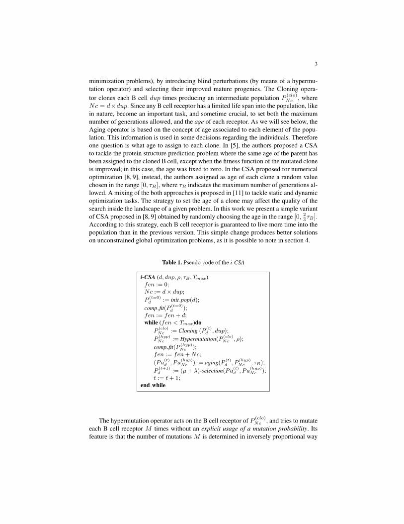
Table 1. Pseudo-code of the i-CSA

i-CSA (d, dup, ρ, τB , Tmax)fen := 0;Nc := d× dup;P

(t=0)d := init pop(d);

comp fit(P (t=0)d );

fen := fen+ d;while (fen < Tmax)do

P(clo)Nc := Cloning (P

(t)d , dup);

P(hyp)Nc := Hypermutation(P

(clo)Nc , ρ);

comp fit(P (hyp)Nc );

fen := fen+Nc;

(Pa(t)d , Pa

(hyp)Nc ) := aging(P

(t)d , P

(hyp)Nc , τB);

P(t+1)d := (µ+ λ)-selection(Pa

(t)d , Pa

(hyp)Nc );

t := t+ 1;end while

The hypermutation operator acts on the B cell receptor of P (clo)Nc , and tries to mutate

each B cell receptor M times without an explicit usage of a mutation probability. Itsfeature is that the number of mutations M is determined in inversely proportional way

4

respect fitness values; as the fitness function value increases, the number of mutationsperformed on it decreases. There are nowadays several different kinds of hypermutationoperators [12] and [13]. The number of mutations M is given by the mutation rate:α = e−ρf(x), where f(x) is the fitness function value normalized in the range [0, 1].As described in [8, 9], the perturbation operator for any receptor x randomly choosesa variable xti, with i ∈ {1, . . . , `} (` is the length of B cell receptor, i.e. the problemdimension), and replace it with

x(t+1)i =

((1− β)× x(t)i

)+(β × x(t)random

),

where x(t)random 6= x(t)i is a randomly chosen variable and β ∈ [0, 1] is a real random

number. All the mutation operators apply a toroidal approach to shrink the variablevalue inside the relative valid region. To normalize the fitness into the range [0, 1], in-stead to use the optimal value of the given function, we have taken into account thebest current fitness value in P td, decreased of an user-defined threshold Θ, as proposedin [8, 9]. This strategy is due to making the algorithm as blind as possible, since is notknown a priori any additional information concerning the problem. The third immuno-logical operator, aging operator, has the main goal to design an high diversity into thecurrent population, and hence avoid premature convergence. It acts on the two popu-lations P (t)

d , and P (hyp)Nc , eliminating all old B cells; when a B cell is τB + 1 old it is

erased from the current population, independently from its fitness value. The parameterτB indicates the maximum number of generations allowed to each B cell receptor toremain into the population. At each generation, the age of each individual is increased.Only one exception is made for the best receptor; when generating a new populationthe selection mechanism does not allow the elimination of the best B cell. After the ag-ing operator is applied, the best survivors from the populations Pa(t)d and Pa(hyp)Nc areselected for the new population P (t+1)

d , of d B cells. If only d1 < d B cells survived,then (µ + λ)-Selection operator (with µ = d and λ = Nc) pick at random d − d1 Bcells among those “died” from the set(

(P(t)d \ Pa

(t)d ) t (P

(hyp)Nc \ Pa(hyp)Nc )

).

Finally, the evolution cycle ends when the fitness evaluation number (fen) is greateror equal to the allowed maximum number of fitness function evaluations, labelled withTmax; fen is a counter that is increased whenever the procedure comp fit(∗) is called.Table 1 summarizes the proposed CSA described above.

3 Kullback-Leibler, Renyi and von Neumann EntropicDivergences

A study on the learning process of i-CSA during the evolution was made, using threedifferent divergence metrics, as Kullback-Leibler, Renyi generalized, and Von Neumanndivergences. These information were obtained both with respect the initial distribution,and the ones in previous step.

5

Shannon’s entropy [15] is a commonly used measure in information theory and itrepresents a good measure of randomness or uncertainty, where the entropy of a randomvariable is defined in terms of its probability distribution. Shannon’s theory, informationis represented by a numerically measurable quantity, using a probabilistic model. In thisway, the solutions of a given problem can be formulated in terms of the obtained amountof information. Kullback-Leibler divergence (KLd) [16], also known as Informationgain, is one of the most frequently used information-theoretic distance measure, basedon two probability distributions of discrete random variable, called relative information,which found many applications in setting important theorems in information theory andstatistics. This divergence measures the quantity of information the system discoversduring the learning phase with respect to the initial population [6].

We define the B cells distribution function f (t)m as the ratio between the number,Btm, of B cells at time step t with fitness function value m, and the total number of Bcells:

f (t)m =Btm∑hm=0B

tm

=Btmd.

The KLd is formally defined as:

KLd(f(t)m , f (t0)m ) =

∑m

f (t)m log

(f(t)m

f(t0)m

).

The gain is the amount of information the system has already learned during its search

0

5

10

15

20

25

1 2 4 8 16 32

Generations

Information Gain

f5f7

f10

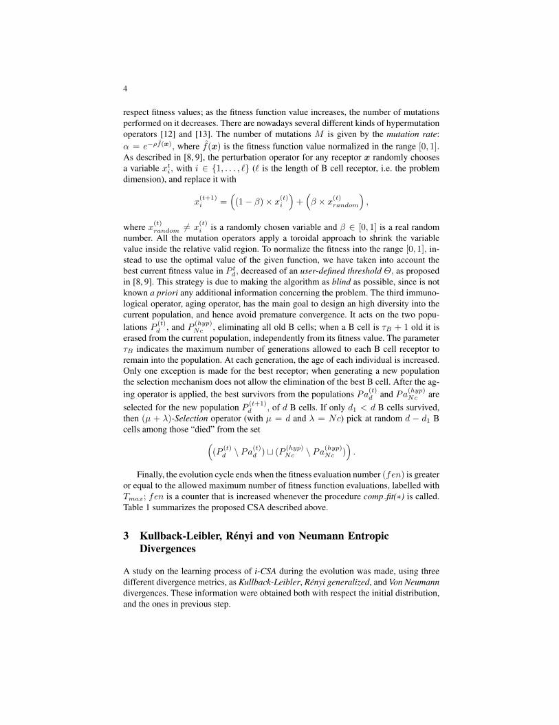
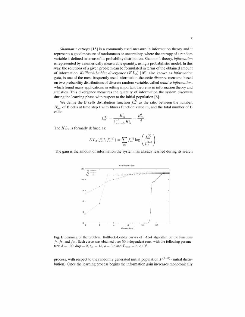
Fig. 1. Learning of the problem. Kullback-Leibler curves of i-CSA algorithm on the functionsf5, f7, and f10. Each curve was obtained over 50 independent runs, with the following parame-ters: d = 100, dup = 2, τB = 15, ρ = 3.5 and Tmax = 5× 105.

process, with respect to the randomly generated initial population P (t=0) (initial distri-bution). Once the learning process begins the information gain increases monotonically

6

until it reaches a final steady state (see figure 1). This is consistent with the idea of amaximum Kullback-Leibler principle [17] of the form: dKLd

dt ≥ 0. Since the learningprocess will end when dKLd

dt = 0, then such maximum principle may be used as ter-mination condition [6, 14]. We are aware that the same metric can be adopted to studythe gain of information regarding the spatial arrangement of the solution in the searchlandscape; in particular, in these terms, when the gain goes to zero it states that theindividuals represent the same solution.

Figure 1 shows the KLd curves obtained by i-CSA, on the functions f5, f7, and f10of the classical benchmark used for our experiments, and proposed in [7]. In this figureone can see as the algorithm gains quickly amounts of information on the functionsf7 and f10, rather than on f5, whose KLd is slower; it starts to gain information aftergeneration number 20. This is due because the search space on f5 seems to be morecomplex than in f7 and f10, and this behavior is consistent with the obtained exper-imental results, where i-CSA, and optimization algorithms in general, need a greaternumber of fitness function evaluations to achieve a good solution. The curves plotted insuch figure were obtained with the following experimental protocol: d = 100, dup = 2,τB = 15, ρ = 3.5 and Tmax = 5× 105. This experiment was performed over 50 inde-pendent runs.

0

5

10

15

20

25

16 32 64

Generations

Clonal Selection Algorithm: i-CSA

0

50

100

150

200

250

300

16 32 64

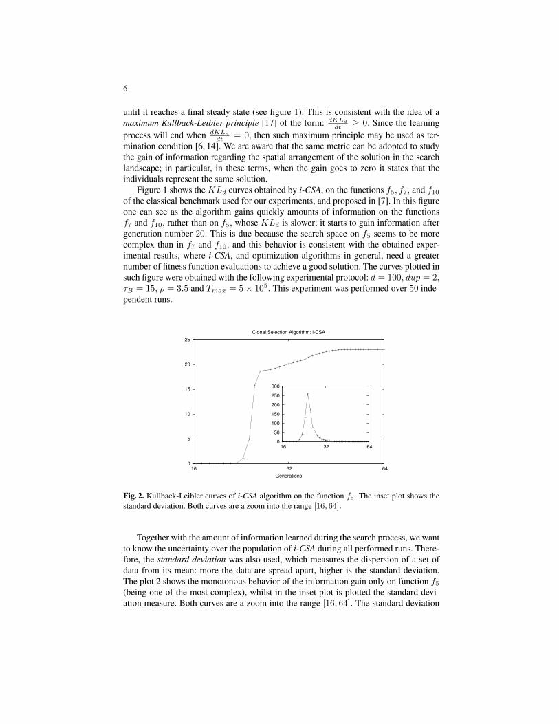
Fig. 2. Kullback-Leibler curves of i-CSA algorithm on the function f5. The inset plot shows thestandard deviation. Both curves are a zoom into the range [16, 64].

Together with the amount of information learned during the search process, we wantto know the uncertainty over the population of i-CSA during all performed runs. There-fore, the standard deviation was also used, which measures the dispersion of a set ofdata from its mean: more the data are spread apart, higher is the standard deviation.The plot 2 shows the monotonous behavior of the information gain only on function f5(being one of the most complex), whilst in the inset plot is plotted the standard devi-ation measure. Both curves are a zoom into the range [16, 64]. The standard deviation

7

increases quickly (the spike in the inset plot) when the algorithm begins to learn infor-mation; once the algorithm begins to gain more information, i.e. after 2− 3 generationsfrom beginning the learning process, the curve of the standard deviation decreases to-wards zero. The algorithm converges to the best solution in this temporal window. Thus,the highest point of information learned corresponds to the lowest value of uncertainty.

0

5e+08

1e+09

1.5e+09

2e+09

2.5e+09

3e+09

3.5e+09

4e+09

0 2 4 6 8 10

Fitn

ess

Generations

Clonal Selection Algorithm: i-CSA

avg fitnessbest fitness

0

5

10

15

20

25

16 32 64

gainentropy

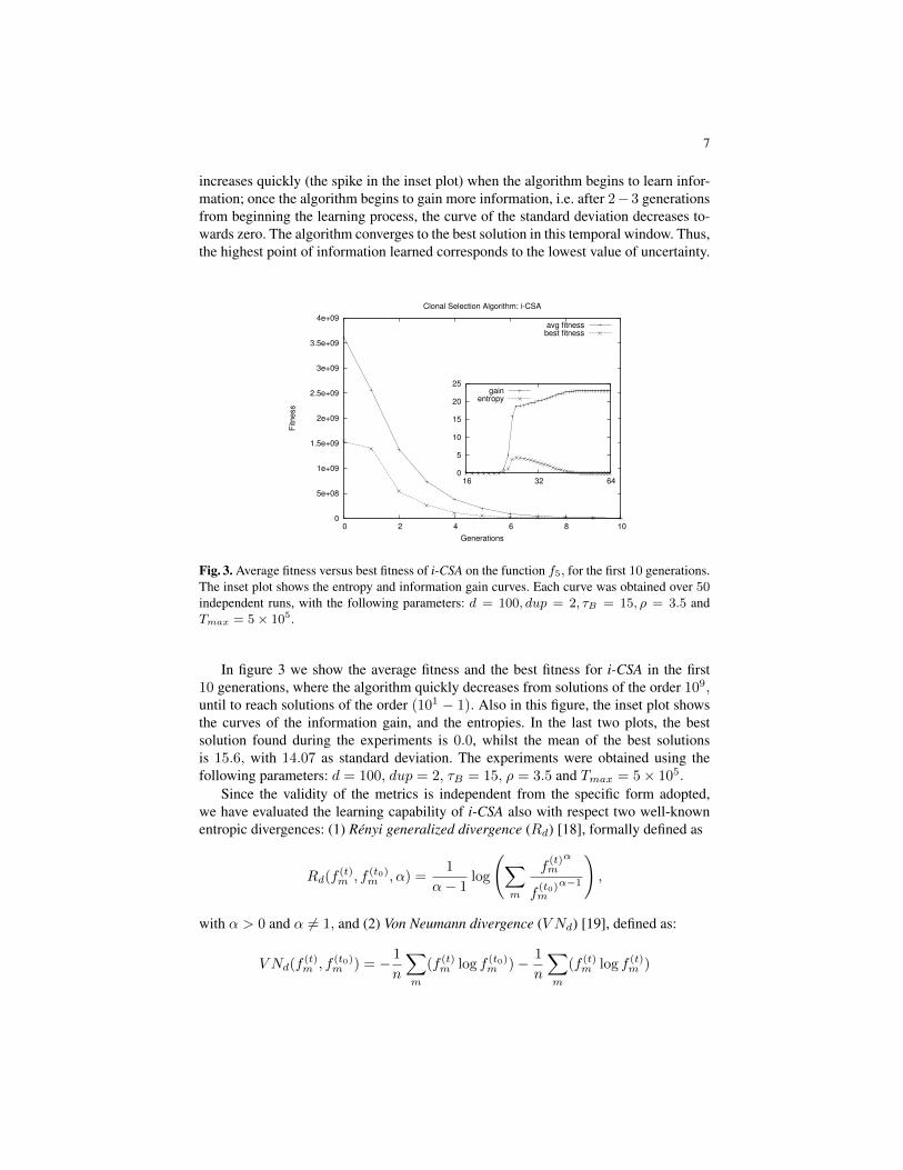
Fig. 3. Average fitness versus best fitness of i-CSA on the function f5, for the first 10 generations.The inset plot shows the entropy and information gain curves. Each curve was obtained over 50independent runs, with the following parameters: d = 100, dup = 2, τB = 15, ρ = 3.5 andTmax = 5× 105.

In figure 3 we show the average fitness and the best fitness for i-CSA in the first10 generations, where the algorithm quickly decreases from solutions of the order 109,until to reach solutions of the order (101 − 1). Also in this figure, the inset plot showsthe curves of the information gain, and the entropies. In the last two plots, the bestsolution found during the experiments is 0.0, whilst the mean of the best solutionsis 15.6, with 14.07 as standard deviation. The experiments were obtained using thefollowing parameters: d = 100, dup = 2, τB = 15, ρ = 3.5 and Tmax = 5× 105.

Since the validity of the metrics is independent from the specific form adopted,we have evaluated the learning capability of i-CSA also with respect two well-knownentropic divergences: (1) Renyi generalized divergence (Rd) [18], formally defined as

Rd(f(t)m , f (t0)m , α) =

1

α− 1log

(∑m

f(t)m

α

f(t0)m

α−1

),

with α > 0 and α 6= 1, and (2) Von Neumann divergence (V Nd) [19], defined as:

V Nd(f(t)m , f (t0)m ) = − 1

n

∑m

(f (t)m log f (t0)m )− 1

n

∑m

(f (t)m log f (t)m )

8

-5

0

5

10

15

20

25

30

16 32 64

Generations

Learning with respect to initial distribution (t0)

Von Neumann distribution (VNd)Renyi generalized

Kullback-Leibler entropy

0

0.2

0.4

0.6

0.8

1

1.2

16 32 64

VNd

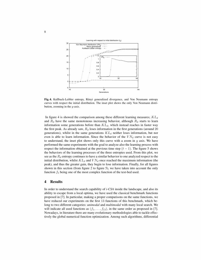
Fig. 4. Kullback-Leibler entropy, Renyi generalized divergence, and Von Neumann entropycurves with respect the initial distribution. The inset plot shows the only Von Neumann distri-bution, zooming in the y-axis.

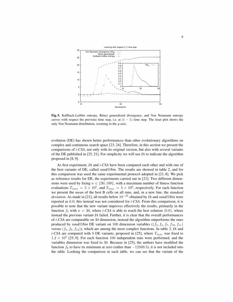
In figure 4 is showed the comparison among these different learning measures; KLdand Rd have the same monotonous increasing behavior, although Rd starts to learninformation some generations before than KLd, which instead reaches in faster waythe first peak. As already saw, Rd loses information in the first generations (around 20generations), whilst in the same generations KLd neither loses information, but noreven is able to learn information. Since the behavior of the V Nd curve is not easyto understand, the inset plot shows only this curve with a zoom in y axis. We haveperformed the same experiments with the goal to analyze also the learning process withrespect the information obtained at the previous time step (t − 1). The figure 5 showsthe behaviors of the learning processes of the three entropies used. From this plot, wesee as theRd entropy continues to have a similar behavior to one analyzed respect to theinitial distribution, whilst KLd and V Nd once reached the maximum information (thepeak), and thus the greater gain, they begin to lose information. Finally, for all figuresshown in this section (from figure 2 to figure 5), we have taken into account the onlyfunction f5 being one of the most complex function of the test-bed used.

4 Results

In order to understand the search capability of i-CSA inside the landscape, and also itsability to escape from a local optima, we have used the classical benchmark functionsproposed in [7]. In particular, making a proper comparisons on the same functions, wehave reduced our experiments on the first 13 functions of this benchmark, which be-long to two different categories: unimodal and multimodal with many local search. Wewill indicate all used functions as (f1, . . . , f13), in the same order as proposed in [7].Nowadays, in literature there are many evolutionary methodologies able to tackle effec-tively the global numerical function optimization. Among such algorithms, differential

9

-5

0

5

10

15

20

25

30

16 32 64

Generations

Learning with respect (t-1) time step

Von Neumann divergence (VNd)Renyi generalized

Kullback-Leibler entropy

0

0.1

0.2

0.3

0.4

0.5

0.6

0.7

0.8

0.9

16 32 64

VNd

Fig. 5. Kullback-Leibler entropy, Renyi generalized divergence, and Von Neumann entropycurves with respect the previous time step, i.e. at (t − 1) time step. The inset plot shows theonly Von Neumann distribution, zooming in the y-axis.

evolution (DE) has shown better performances than other evolutionary algorithms oncomplex and continuous search space [23, 24]. Therefore, in this section we present thecomparisons of i-CSA, not only with its original version, but also with several variantsof the DE published in [25, 21]. For simplicity we will use IA to indicate the algorithmproposed in [8, 9].

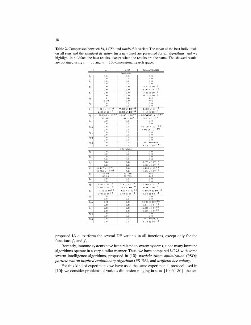
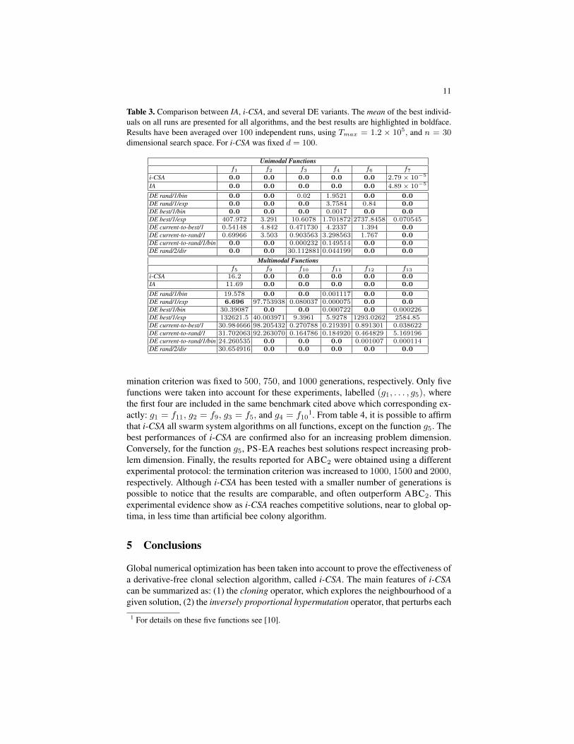
As first experiment, IA and i-CSA have been compared each other and with one ofthe best variants of DE, called rand/1/bin. The results are showed in table 2, and forthis comparison was used the same experimental protocol adopted in [21, 8]. We pickas reference results for DE, the experiments carried out in [21]. Two different dimen-sions were used by fixing n ∈ {30, 100}, with a maximum number of fitness functionevaluations Tmax = 5 × 105, and Tmax = 5 × 106, respectively. For each functionwe present the mean of the best B cells on all runs, and, in a new line, the standarddeviation. As made in [21], all results below 10−25 obtained by IA and rand/1/bin werereported as 0.0; this instead was not considered for i-CSA. From this comparison, it ispossible to note that the new variant improves effectively the results, primarily in thefunction f5 with n = 30, where i-CSA is able to reach the best solution (0.0), whereinstead the previous variant IA failed. Further, it is clear that the overall performancesof i-CSA are comparable on 30 dimension, instead the algorithm outperforms the onesproduced by rand/1/bin DE variant on 100 dimension variables ((f3, f4, f7, f10, f11)versus (f5, f8, f13)), which are among the most complex functions. In table 3, IA andi-CSA are compared with 8 DE variants, proposed in [25], where Tmax was fixed to1.2 × 105 [25, 9]. For each function 100 independent runs were performed, and thevariables dimension was fixed to 30. Because in [25], the authors have modified thefunction f8 to have its minimum at zero (rather than −12569.5), it is not included intothe table. Looking the comparison in such table, we can see that the variant of the

10

Table 2. Comparison between IA, i-CSA and rand/1/bin variant The mean of the best individualson all runs and the standard deviation (in a new line) are presented for all algorithms, and wehighlight in boldface the best results, except when the results are the same. The showed resultsare obtained using n = 30 and n = 100 dimensional search space.

IA i-CSA DE rand/1/bin [21]

30 variablesf1 0.0 0.0 0.0

0.0 0.0 0.0

f2 0.0 0.0 0.00.0 0.0 0.0

f3 0.0 0.0 2.02 × 10−9

0.0 0.0 8.26 × 10−10

f4 0.0 0.0 3.85 × 10−8

0.0 0.0 9.17 × 10−9

f5 12 0.0 0.013.22 0.0 0.0

f6 0.0 0.0 0.00.0 0.0 0.0

f7 1.521 × 10−5 7.48 × 10−6 4.939 × 10−3

2.05 × 10−5 6.46 × 10−6 1.13 × 10−3

f8 −1.256041 × 10+4 −9.05 × 10+3 −1.256948 × 10+4

25.912 1.91 × 104 2.3 × 10−4

f9 0.0 0.0 0.00.0 0.0 0.0

f10 0.0 0.0 −1.19 × 10−15

0.0 0.0 7.03 × 10−16

f11 0.0 0.0 0.00.0 0.0 0.0

f12 0.0 0.0 0.00.0 0.0 0.0

f13 0.0 0.0 −1.142824

0.0 0.0 4.45 × 10−8

100 variablesf1 0.0 0.0 0.0

0.0 0.0 0.0

f2 0.0 0.0 0.00.0 0.0 0.0

f3 0.0 0.0 5.87 × 10−10

0.0 0.0 1.83 × 10−10

f4 6.447 × 10−7 0.0 1.128 × 10−9

3.338 × 10−6 0.0 1.42 × 10−10

f5 74.99 22.116 0.038.99 39.799 0.0

f6 0.0 0.0 0.00.0 0.0 0.0

f7 1.59 × 10−5 1.2 × 10−6 7.664 × 10−3

3.61 × 10−5 1.53 × 10−6 6.58 × 10−4

f8 −4.16 × 10+4 −2.727 × 10+4 −4.1898 × 10+4

2.06 × 10+2 7.63 × 10−4 1.06 × 10−3

f9 0.0 0.0 0.00.0 0.0 0.0

f10 0.0 0.0 8.023 × 10−15

0.0 0.0 1.74 × 10−15

f11 0.0 0.0 5.42 × 10−20

0.0 0.0 5.42 × 10−20

f12 0.0 0.0 0.00.0 0.0 0.0

f13 0.0 0.0 −1.142824

0.0 0.0 2.74 × 10−8

proposed IA outperform the several DE variants in all functions, except only for thefunctions f5 and f7.

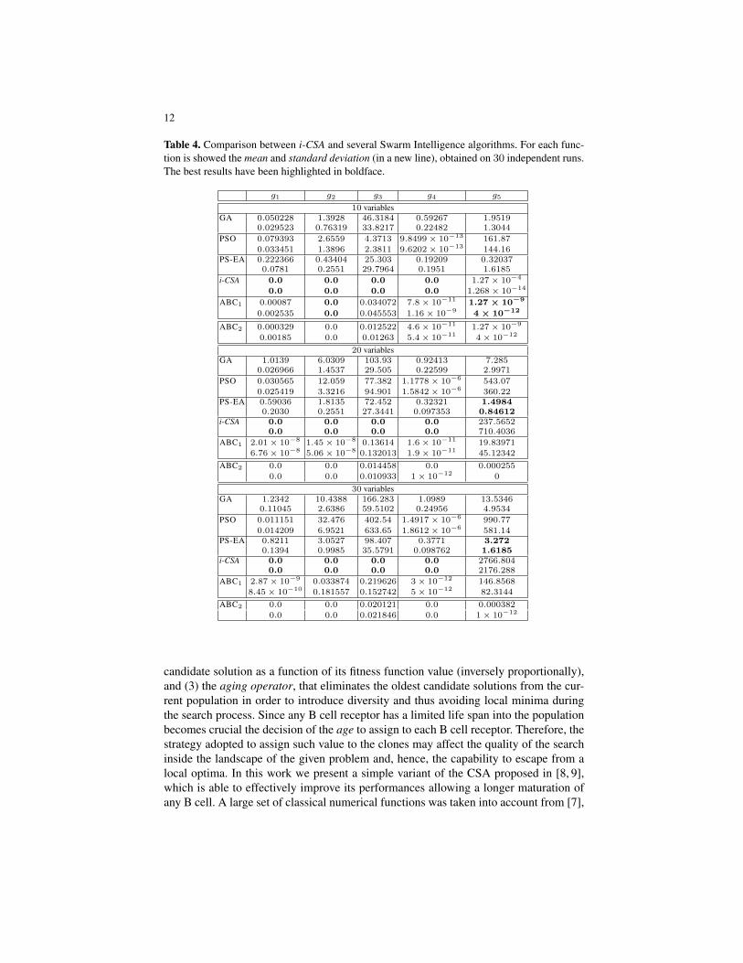
Recently, immune systems have been related to swarm systems, since many immunealgorithms operate in a very similar manner. Thus, we have compared i-CSA with someswarm intelligence algorithms, proposed in [10]: particle swam optimization (PSO);particle swarm inspired evolutionary algorithm (PS-EA), and artificial bee colony.

For this kind of experiments we have used the same experimental protocol used in[10]; we consider problems of various dimension ranging in n = {10, 20, 30}; the ter-

11

Table 3. Comparison between IA, i-CSA, and several DE variants. The mean of the best individ-uals on all runs are presented for all algorithms, and the best results are highlighted in boldface.Results have been averaged over 100 independent runs, using Tmax = 1.2 × 105, and n = 30dimensional search space. For i-CSA was fixed d = 100.

Unimodal Functionsf1 f2 f3 f4 f6 f7

i-CSA 0.0 0.0 0.0 0.0 0.0 2.79 × 10−5

IA 0.0 0.0 0.0 0.0 0.0 4.89 × 10−5

DE rand/1/bin 0.0 0.0 0.02 1.9521 0.0 0.0DE rand/1/exp 0.0 0.0 0.0 3.7584 0.84 0.0DE best/1/bin 0.0 0.0 0.0 0.0017 0.0 0.0DE best/1/exp 407.972 3.291 10.6078 1.701872 2737.8458 0.070545DE current-to-best/1 0.54148 4.842 0.471730 4.2337 1.394 0.0DE current-to-rand/1 0.69966 3.503 0.903563 3.298563 1.767 0.0DE current-to-rand/1/bin 0.0 0.0 0.000232 0.149514 0.0 0.0DE rand/2/dir 0.0 0.0 30.112881 0.044199 0.0 0.0

Multimodal Functionsf5 f9 f10 f11 f12 f13

i-CSA 16.2 0.0 0.0 0.0 0.0 0.0IA 11.69 0.0 0.0 0.0 0.0 0.0

DE rand/1/bin 19.578 0.0 0.0 0.001117 0.0 0.0DE rand/1/exp 6.696 97.753938 0.080037 0.000075 0.0 0.0DE best/1/bin 30.39087 0.0 0.0 0.000722 0.0 0.000226DE best/1/exp 132621.5 40.003971 9.3961 5.9278 1293.0262 2584.85DE current-to-best/1 30.984666 98.205432 0.270788 0.219391 0.891301 0.038622DE current-to-rand/1 31.702063 92.263070 0.164786 0.184920 0.464829 5.169196DE current-to-rand/1/bin 24.260535 0.0 0.0 0.0 0.001007 0.000114DE rand/2/dir 30.654916 0.0 0.0 0.0 0.0 0.0

mination criterion was fixed to 500, 750, and 1000 generations, respectively. Only fivefunctions were taken into account for these experiments, labelled (g1, . . . , g5), wherethe first four are included in the same benchmark cited above which corresponding ex-actly: g1 = f11, g2 = f9, g3 = f5, and g4 = f10

1. From table 4, it is possible to affirmthat i-CSA all swarm system algorithms on all functions, except on the function g5. Thebest performances of i-CSA are confirmed also for an increasing problem dimension.Conversely, for the function g5, PS-EA reaches best solutions respect increasing prob-lem dimension. Finally, the results reported for ABC2 were obtained using a differentexperimental protocol: the termination criterion was increased to 1000, 1500 and 2000,respectively. Although i-CSA has been tested with a smaller number of generations ispossible to notice that the results are comparable, and often outperform ABC2. Thisexperimental evidence show as i-CSA reaches competitive solutions, near to global op-tima, in less time than artificial bee colony algorithm.

5 Conclusions

Global numerical optimization has been taken into account to prove the effectiveness ofa derivative-free clonal selection algorithm, called i-CSA. The main features of i-CSAcan be summarized as: (1) the cloning operator, which explores the neighbourhood of agiven solution, (2) the inversely proportional hypermutation operator, that perturbs each

1 For details on these five functions see [10].

12

Table 4. Comparison between i-CSA and several Swarm Intelligence algorithms. For each func-tion is showed the mean and standard deviation (in a new line), obtained on 30 independent runs.The best results have been highlighted in boldface.

g1 g2 g3 g4 g5

10 variablesGA 0.050228 1.3928 46.3184 0.59267 1.9519

0.029523 0.76319 33.8217 0.22482 1.3044

PSO 0.079393 2.6559 4.3713 9.8499 × 10−13 161.87

0.033451 1.3896 2.3811 9.6202 × 10−13 144.16PS-EA 0.222366 0.43404 25.303 0.19209 0.32037

0.0781 0.2551 29.7964 0.1951 1.6185

i-CSA 0.0 0.0 0.0 0.0 1.27 × 10−4

0.0 0.0 0.0 0.0 1.268 × 10−14

ABC1 0.00087 0.0 0.034072 7.8 × 10−11 1.27 × 10−9

0.002535 0.0 0.045553 1.16 × 10−9 4 × 10−12

ABC2 0.000329 0.0 0.012522 4.6 × 10−11 1.27 × 10−9

0.00185 0.0 0.01263 5.4 × 10−11 4 × 10−12

20 variablesGA 1.0139 6.0309 103.93 0.92413 7.285

0.026966 1.4537 29.505 0.22599 2.9971

PSO 0.030565 12.059 77.382 1.1778 × 10−6 543.07

0.025419 3.3216 94.901 1.5842 × 10−6 360.22PS-EA 0.59036 1.8135 72.452 0.32321 1.4984

0.2030 0.2551 27.3441 0.097353 0.84612i-CSA 0.0 0.0 0.0 0.0 237.5652

0.0 0.0 0.0 0.0 710.4036

ABC1 2.01 × 10−8 1.45 × 10−8 0.13614 1.6 × 10−11 19.83971

6.76 × 10−8 5.06 × 10−8 0.132013 1.9 × 10−11 45.12342

ABC2 0.0 0.0 0.014458 0.0 0.000255

0.0 0.0 0.010933 1 × 10−12 0

30 variablesGA 1.2342 10.4388 166.283 1.0989 13.5346

0.11045 2.6386 59.5102 0.24956 4.9534

PSO 0.011151 32.476 402.54 1.4917 × 10−6 990.77

0.014209 6.9521 633.65 1.8612 × 10−6 581.14PS-EA 0.8211 3.0527 98.407 0.3771 3.272

0.1394 0.9985 35.5791 0.098762 1.6185i-CSA 0.0 0.0 0.0 0.0 2766.804

0.0 0.0 0.0 0.0 2176.288

ABC1 2.87 × 10−9 0.033874 0.219626 3 × 10−12 146.8568

8.45 × 10−10 0.181557 0.152742 5 × 10−12 82.3144

ABC2 0.0 0.0 0.020121 0.0 0.000382

0.0 0.0 0.021846 0.0 1 × 10−12

candidate solution as a function of its fitness function value (inversely proportionally),and (3) the aging operator, that eliminates the oldest candidate solutions from the cur-rent population in order to introduce diversity and thus avoiding local minima duringthe search process. Since any B cell receptor has a limited life span into the populationbecomes crucial the decision of the age to assign to each B cell receptor. Therefore, thestrategy adopted to assign such value to the clones may affect the quality of the searchinside the landscape of the given problem and, hence, the capability to escape from alocal optima. In this work we present a simple variant of the CSA proposed in [8, 9],which is able to effectively improve its performances allowing a longer maturation ofany B cell. A large set of classical numerical functions was taken into account from [7],

13

which is divided into two different categories: unimodal and multimodal (with many lo-cal optima) functions. i-CSA was compared with several variants of the DE algorithm,since it has been shown to be effective on many optimization problems. Afterwards, be-cause nowadays immunological systems are considered similar to swarm systems, wehave compared i-CSA with state-of-the-art swarm algorithms. The analysis of the resultsshows that i-CSA is comparable, and often outperforms, all nature-inspired algorithmsin terms of accuracy to the accuracy, and effectiveness in solving large-scale instances.By analyzing one of the most difficult function of the benchmark, (f5), we characterizethe learning capability of i-CSA. The obtained gain has been analyzed both with respectthe initial distribution, and the ones obtained in the previous step. For this study, threedifferent entropic metrics were used, as Kullback-Leibler, Renyi and von Neumann di-vergences [16, 18, 19]. By the relative curves, is possible to observe a strong correlationbetween optima (peaks in the search landscape) discovering, and high relative entropyvalues.

References

1. J. Timmis, A. Hone, T. Stibor, E. Clark: “Theoretical advances in artificial immune systems”,Theoretical Computer Science, vol. 403, no. 1, pp. 11–32, 2008.

2. S. Smith, J. Timmis: “An Immune Network Inspired Evolutionary Algorithm for the Diagno-sis of Parkinsons Disease”, Biosystems, vol. 94, no. (1–2), pp. 34–46, 2008.

3. J. Timmis, E. Hart, A. Hone, M. Neal, A. Robins, S. Stepney, A. Tyrrell: “Immuno-Engineering”, in Proc. of the international conference on Biologically Inspired CollaborativeComputing (IFIP’09), IEEE Press, vol. 268, pp. 3–17, 2008.

4. D. Dasgupta, F. Nino: “Immunological Computation: Theory and Applications”, CRC Press(in press).

5. V. Cutello, G. Nicosia, M. Pavone, J. Timmis: ”An Immune Algorithm for Protein StructurePrediction on Lattice Models”, IEEE Trans. on Evolutionary Computation, vol. 11, no. 1, pp.101–117, 2007.

6. V. Cutello, G. Nicosia, M. Pavone: ”An immune algorithm with stochastic aging and kullbackentropy for the chromatic number problem”, Journal of Combinatorial Optimization, vol. 14,no. 1, pp. 9-33, 2007.

7. X. Yao, Y. Liu, G. M. Lin: “Evolutionary programming made faster”, IEEE Trans. on Evo-lutionary Computation, vol. 3, no. 2, pp. 82–102, 1999.

8. V. Cutello, G. Nicosia, M. Pavone, G. Narzisi: “Real Coded Clonal Selection Algorithmfor Unconstrained Global Numerical Optimization using a Hybrid Inversely ProportionalHypermutation Operator”, in Proc. of the 21st Annual ACM Symposium on Applied Com-puting (SAC’06), vol. 2, pp. 950–954, 2006.

9. V. Cutello, N. Krasnogor, G. Nicosia, M. Pavone; “Immune Algorithm versus DifferentialEvolution: A Comparative Case Study Using High Dimensional Function Optimization”,in Proc. of the International Conference on Adaptive and Natural Computing Algorithms(ICANNGA’07), LNCS, vol. 4431, pp. 93–101, 2007.

10. D. Karaboga, B. Baturk: “A powerful and efficient algorithm for numerical function opti-mization: artificial bee colony (ABC) algorithm”, Journal of Global Optimization, vol. 39,pp. 459–471, 2007.

11. M. Castrogiovanni, G. Nicosia, R. Rascuna ”Experimental Analysis of the Aging Operatorfor Static and Dynamic Optimisation Problems”, in Proc. of the 11th International Confer-ence on Knowledge-Based and Intelligent Information and Engineering Systems (KES’07),LNCS, vol. 4694, pp. 804–811, 2007.

14

12. V. Cutello, G. Nicosia, M. Pavone: “Exploring the capability of immune algorithms: a char-acterization of hypermutation operators”, in Proc. of the Third International Conference onArtificial Immune Systems (ICARIS’04), LNCS, vol. 3239, pp. 263–276, 2004.

13. V. Cutello, G. Nicosia, M. Pavone: “An Immune Algorithm with Hyper-Macromutations forthe Dill’s 2D Hydrophobic-Hydrophilic Model”, in Proc. of Congress on Evolutionary Com-putation (CEC’04), IEEE Press, vol. 1, pp. 1074–1080, 2004.

14. V. Cutello, G. Nicosia, M. Pavone: “A Hybrid Immune Algorithm with Information Gain forthe Graph Coloring Problem”, in Proc. of Genetic and Evolutionary Computation COnfer-ence (GECCO’03), LNCS 2723, pp. 171–182, 2003.

15. C. E. Shannon: ”A Mathematical Theory of Communication”, Congress on EvolutionaryComputation, Vol. 1, pp. 1074–1080, IEEE Press (2004) Bell System Technical Journal, Vol.27, pp. 379–423 and 623–656 (1948)

16. S. Kullback S.: ”Statistics and Information Theory”, J. Wiley and Sons, New York (1959)17. Jaynes E.: ”Probability Theory: The Logic of Science”, Cambridge University Press, 2003.18. A. Renyi: ”On measures of information and entropy”, in Proc. of the 4th Berkeley Sympo-

sium on Mathematics, Statistics and Probability, pp. 547–561, 1961.19. A. Kopp, X. Jia, S. Chakravarty: ”Replacing energy by von Neumann entropy in quantum

phase transitions”, Annals of Physics, vol. 322, no. 6, pp. 1466–1476, 2007.20. V. Cutello, G. Narzisi, G. Nicosia, M. Pavone: “Clonal Selection Algorithms: A Compar-

ative Case Study using Effective Mutation Potentials”, in Proc. of the Fourth InternationalConference on Artificial Immune Systems (ICARIS’05), LNCS, vol. 3627, pp. 13–28, 2005.

21. J. Versterstrøm, R. Thomsen: ”A Comparative Study of Differential Evolution, ParticleSwarm Optimization, and Evolutionary Algorithms on Numerical Benchmark Problems”,in Congress on Evolutionary Computing (CEC’04), vol. 1, pp. 1980–1987, 2004.

22. N. Noman, H. Iba: ”Enhancing Differential Evolution Performance with Local Search forHigh Dimensional Function Optimization”, in Genetic and Evolutionary Computation Con-ference (GECCO’05), pp. 967–974, 2005.

23. R. Storn, K. V. Price: ”Differential Evolution a Simple and Efficient Heuristic for GlobalOptimization over Continuous Spaces”, Journal of Global Optimization, vol. 11, no. 4, pp.341–359, 1997.

24. K. V. Price, M. Storn, J. A. Lampien: ”Differential Evolution: A Practical Approach toGlobal Optimization”, Springer-Verlag, 2005.

25. E. Mezura–Montes, J. Velazquez–Reyes, C. Coello Coello: ”A Comparative Study of Differ-ential Evolution Variants for Global Optimization”, in Genetic and Evolutionary Computa-tion Conference (GECCO’06), vol. 1, pp. 485–492, 2006.