Embed Size (px)
Citation preview

John J. Cannon Catherine Playoust
School of Mathematics and Statistics, University of Sydney
An Introduction toAlgebraic Programming withMagma (Draft)
Volume I: The Magma Language
Volume II: The Magma Categories
February 16, 2001
Springer-Verlag
Berlin Heidelberg NewYorkLondon Paris TokyoHongKong BarcelonaBudapest

Copyright c©1996. All rights reserved.No part of this book may be reproduced without written permission.
Typeset in the LATEX macro package CLMono01 developed by Springer-Verlag Heidelberg as a free service to its authors and editors preparingcamera-ready copy.

Preface
What Is Magma?
Magma is a programming language designed for the investigation of alge-braic, geometric and combinatorial structures, or magmas. The syntax of thelanguage resembles that of many well-known programming languages. Whatis special about Magma is the provision of mathematical data types suchas groups, rings, fields, sets, sequences and mappings, together with a largecollection of functions for performing standard tasks in algebra. Informationabout the magmas and their elements is stored in a mathematically powerfulway, making advanced symbolic algebraic computation feasible. Magma is asophisticated tool for experimentation, education, and computer-aided proof,useful for both students and professional mathematicians.
About This Book
This book is an introductory manual for Magma. It presumes no knowledgeof computer programming, and its examples are chosen to illustrate languageand algorithmic features as simply as possible. Volume I explains the lan-guage and user environment in detail, and Volume II deals with the majoralgebraic, geometrical and combinatorial structures implemented in the sys-tem. Note carefully that this book does not attempt to give comprehensivecoverage of the algorithms implemented in Magma. Before undertaking se-rious computations in Magma, the user should also consult the referencemanual, Handbook of Magma Functions [BoC96]; within the present book, itis referred to simply as Handbook.
Although this book is designed as an introduction, the short bookletFirst Steps in Magma may be more appropriate for those requiring only apassing acquaintance with the system.

VI
System Updates and Release Notes
The version of the system documented in this edition is Magma V2, releasedin 1996. Release notes for later versions may be obtained from the developersof Magma.
Acknowledgements
Many people assisted us in the writing of this book. We would particularlylike to thank Wieb Bosma and Allan Steel, who wrote early versions of thechapters on number fields and polynomial rings, respectively, and the currentmembers of the Computational Algebra Group for their valiant proof-reading.
We also wish to thank our families for their support.
Computational Algebra GroupSchool of Mathematics and StatisticsUniversity of SydneyNSW 2006Australia
Email: [email protected]: +61–2–9351–3338Fax: +61–2–9351–4534Home Page:http://www.maths.usyd.edu.au:8000/comp/magma/Overview.html
Sydney, September 1996 John J. Cannon, Catherine Playoust

Table of Contents
Preface . . . . . . . . . . . . . . . . . . . . . . . . . . . . . . . . . . . . . . . . . . . . . . . . . . . . . . . V
Part I. Overview
1. Getting Started With Magma . . . . . . . . . . . . . . . . . . . . . . . . . . . . . 31.1 Entering the Magma System . . . . . . . . . . . . . . . . . . . . . . . . . . . . 31.2 Input and Output . . . . . . . . . . . . . . . . . . . . . . . . . . . . . . . . . . . . . . 31.3 Creating Structures and Their Elements . . . . . . . . . . . . . . . . . . . 41.4 Online Help and Environment . . . . . . . . . . . . . . . . . . . . . . . . . . . . 51.5 Quitting Magma . . . . . . . . . . . . . . . . . . . . . . . . . . . . . . . . . . . . . . . 5
2. Developed Examples . . . . . . . . . . . . . . . . . . . . . . . . . . . . . . . . . . . . . . 72.1 Affine Plane from a Projective Plane by Derivation . . . . . . . . . 72.2 Constructing an Endo-trivial Module . . . . . . . . . . . . . . . . . . . . . 92.3 Molien Series and Primary Invariants . . . . . . . . . . . . . . . . . . . . . 132.4 Galois Group and Action . . . . . . . . . . . . . . . . . . . . . . . . . . . . . . . . 16
Part II. The Language
3. Basic Ideas . . . . . . . . . . . . . . . . . . . . . . . . . . . . . . . . . . . . . . . . . . . . . . . 233.1 Evaluating and Printing Expressions . . . . . . . . . . . . . . . . . . . . . . 23
3.1.1 Arithmetic . . . . . . . . . . . . . . . . . . . . . . . . . . . . . . . . . . . . . . 243.1.2 Function Calls . . . . . . . . . . . . . . . . . . . . . . . . . . . . . . . . . . . 253.1.3 Printing Text . . . . . . . . . . . . . . . . . . . . . . . . . . . . . . . . . . . . 26
3.2 Identifiers . . . . . . . . . . . . . . . . . . . . . . . . . . . . . . . . . . . . . . . . . . . . . 263.2.1 Labelling Information . . . . . . . . . . . . . . . . . . . . . . . . . . . . . 263.2.2 Showing All Identifiers and Their Values . . . . . . . . . . . . 283.2.3 Deletion and Unassigned Identifiers . . . . . . . . . . . . . . . . . 28
3.3 Assignment . . . . . . . . . . . . . . . . . . . . . . . . . . . . . . . . . . . . . . . . . . . . 293.3.1 The Simple Assignment Statement . . . . . . . . . . . . . . . . . 293.3.2 The Mutation Assignment Statement . . . . . . . . . . . . . . . 31

VIII Table of Contents
3.3.3 Multi-Valued Expressions and the Multiple Assign-ment Statement . . . . . . . . . . . . . . . . . . . . . . . . . . . . . . . . . . 31
3.4 The where-construction . . . . . . . . . . . . . . . . . . . . . . . . . . . . . . . . 333.5 Integers, Rationals, Reals, and Complex Numbers . . . . . . . . . . 353.6 Booleans . . . . . . . . . . . . . . . . . . . . . . . . . . . . . . . . . . . . . . . . . . . . . . 373.7 Comments . . . . . . . . . . . . . . . . . . . . . . . . . . . . . . . . . . . . . . . . . . . . . 403.8 Recalling Previously Printed Values . . . . . . . . . . . . . . . . . . . . . . . 403.9 Loading Input from a File . . . . . . . . . . . . . . . . . . . . . . . . . . . . . . . 42
4. Algebraic Structures . . . . . . . . . . . . . . . . . . . . . . . . . . . . . . . . . . . . . . 454.1 Magmas, Categories and Varieties . . . . . . . . . . . . . . . . . . . . . . . . 454.2 Creation of Magmas . . . . . . . . . . . . . . . . . . . . . . . . . . . . . . . . . . . . 484.3 Automatically-Created Magmas . . . . . . . . . . . . . . . . . . . . . . . . . . 494.4 Creating a Free Magma . . . . . . . . . . . . . . . . . . . . . . . . . . . . . . . . . 504.5 Creating and Operating on Elements of a Magma. . . . . . . . . . . 51
4.5.1 Creating Literal Elements . . . . . . . . . . . . . . . . . . . . . . . . . 524.5.2 Arithmetic Operators . . . . . . . . . . . . . . . . . . . . . . . . . . . . . 544.5.3 Relational Operators . . . . . . . . . . . . . . . . . . . . . . . . . . . . . . 564.5.4 Canonical Forms of Elements . . . . . . . . . . . . . . . . . . . . . . 574.5.5 Generators and Element Representation . . . . . . . . . . . . . 58
4.6 Submagmas, Normal Closures and Ideals . . . . . . . . . . . . . . . . . . 604.6.1 Creating Submagmas and Ideals . . . . . . . . . . . . . . . . . . . . 614.6.2 The Embedding in the Free Magma . . . . . . . . . . . . . . . . . 634.6.3 Inclusion Monomorphism and Principle of Locality . . . 64
4.7 Magma Generators . . . . . . . . . . . . . . . . . . . . . . . . . . . . . . . . . . . . . 664.7.1 Generating Sets . . . . . . . . . . . . . . . . . . . . . . . . . . . . . . . . . . 664.7.2 Determination of the Generators . . . . . . . . . . . . . . . . . . . 684.7.3 Remarks on Generator Names . . . . . . . . . . . . . . . . . . . . . 724.7.4 The Pseudo-Identifier $ . . . . . . . . . . . . . . . . . . . . . . . . . . . 74
4.8 Quotient Magmas . . . . . . . . . . . . . . . . . . . . . . . . . . . . . . . . . . . . . . 754.9 Shorthand Constructors . . . . . . . . . . . . . . . . . . . . . . . . . . . . . . . . . 78
4.9.1 Finitely-Presented Magmas . . . . . . . . . . . . . . . . . . . . . . . . 784.9.2 Submagmas of Generic Magmas . . . . . . . . . . . . . . . . . . . . 81
4.10 Some Other Operations on Magmas . . . . . . . . . . . . . . . . . . . . . . . 824.11 Warning About Large Magmas . . . . . . . . . . . . . . . . . . . . . . . . . . . 85
5. Conditional Statements and Expressions . . . . . . . . . . . . . . . . . . 875.1 The if-statement . . . . . . . . . . . . . . . . . . . . . . . . . . . . . . . . . . . . . . . 87
5.1.1 Basic Form of the if-statement . . . . . . . . . . . . . . . . . . . . . 875.1.2 Special Prompt Symbols . . . . . . . . . . . . . . . . . . . . . . . . . . 885.1.3 Short Form of the if-statement . . . . . . . . . . . . . . . . . . . . . 895.1.4 Avoiding Nested if-statements . . . . . . . . . . . . . . . . . . . . . 895.1.5 Longer Example: Area of a Triangle . . . . . . . . . . . . . . . . 90
5.2 The select-expression . . . . . . . . . . . . . . . . . . . . . . . . . . . . . . . . . . . 925.3 The case-statement . . . . . . . . . . . . . . . . . . . . . . . . . . . . . . . . . . . . 92

Table of Contents IX
5.4 The case-expression . . . . . . . . . . . . . . . . . . . . . . . . . . . . . . . . . . . . 94
6. Aggregate Structures . . . . . . . . . . . . . . . . . . . . . . . . . . . . . . . . . . . . . 976.1 Properties of the Aggregate Categories . . . . . . . . . . . . . . . . . . . . 976.2 Construction of Iterable Homogeneous Aggregates . . . . . . . . . . 100
6.2.1 Construction from an Element-List . . . . . . . . . . . . . . . . . 1006.2.2 The Universe of a Homogeneous Aggregate . . . . . . . . . . 1026.2.3 Empty and Null Sets and Sequences . . . . . . . . . . . . . . . . 1046.2.4 Construction of Arithmetic Progressions . . . . . . . . . . . . . 1056.2.5 Construction from an Element-Description . . . . . . . . . . . 1076.2.6 Recursive Definition of Enumerated Sequences . . . . . . . 1126.2.7 Enumerated Sequences with Undefined Terms . . . . . . . . 113
6.3 Operations on Iterable Homogeneous Aggregates . . . . . . . . . . . 1146.3.1 Index Position, Cardinality and Length . . . . . . . . . . . . . 1146.3.2 Testing Equality, Membership, and Subsetness . . . . . . . 1156.3.3 Including or Excluding an Element . . . . . . . . . . . . . . . . . 1166.3.4 Maximum and Minimum Elements . . . . . . . . . . . . . . . . . 1166.3.5 Reduction . . . . . . . . . . . . . . . . . . . . . . . . . . . . . . . . . . . . . . . 117
6.4 Further Operations on Set Categories . . . . . . . . . . . . . . . . . . . . . 1186.5 Further Operations on Enumerated Sequences . . . . . . . . . . . . . . 120
6.5.1 Changing a Term of a Sequence . . . . . . . . . . . . . . . . . . . . 1216.5.2 Obtaining Several Terms of a Sequence . . . . . . . . . . . . . . 1216.5.3 Subsequences and Concatenation . . . . . . . . . . . . . . . . . . . 1226.5.4 Inserting and Removing Objects . . . . . . . . . . . . . . . . . . . . 1236.5.5 Rearranging the Terms of a Sequence . . . . . . . . . . . . . . . 1246.5.6 Multi-Dimensional Sequences . . . . . . . . . . . . . . . . . . . . . . 125
6.6 Representative and Random Elements . . . . . . . . . . . . . . . . . . . . . 1266.7 Existential and Universal Quantifiers . . . . . . . . . . . . . . . . . . . . . . 1276.8 Creating and Operating on Formal Sets . . . . . . . . . . . . . . . . . . . 1296.9 Lists . . . . . . . . . . . . . . . . . . . . . . . . . . . . . . . . . . . . . . . . . . . . . . . . . . 1306.10 Cartesian Products and Tuples . . . . . . . . . . . . . . . . . . . . . . . . . . . 1326.11 Coproducts . . . . . . . . . . . . . . . . . . . . . . . . . . . . . . . . . . . . . . . . . . . . 1366.12 Record Formats and Records . . . . . . . . . . . . . . . . . . . . . . . . . . . . . 141
6.12.1 Creating Record Formats and Records . . . . . . . . . . . . . . 1416.12.2 Example: Using a Function to Create Records . . . . . . . . 143
6.13 Transfer Functions Between Aggregates . . . . . . . . . . . . . . . . . . . 146
7. Mappings and Homomorphisms . . . . . . . . . . . . . . . . . . . . . . . . . . . 1497.1 Standard Mappings . . . . . . . . . . . . . . . . . . . . . . . . . . . . . . . . . . . . . 1507.2 Operations on Mappings and Homomorphisms . . . . . . . . . . . . . 152
7.2.1 Calculating Images . . . . . . . . . . . . . . . . . . . . . . . . . . . . . . . 1527.2.2 Calculating Preimages . . . . . . . . . . . . . . . . . . . . . . . . . . . . 1547.2.3 Functions on Mappings and Homomorphisms . . . . . . . . 156
7.3 Constructing Mappings and Homomorphisms . . . . . . . . . . . . . . 1567.3.1 Mapping Rule Given as Expression . . . . . . . . . . . . . . . . . 157

X Table of Contents
7.3.2 Element-by-Element Rule for General Mappings . . . . . . 1607.3.3 Generator-Image Mapping Rule for Homomorphisms . . 161
7.4 Composing Mappings . . . . . . . . . . . . . . . . . . . . . . . . . . . . . . . . . . . 1637.5 Recursive Definitions . . . . . . . . . . . . . . . . . . . . . . . . . . . . . . . . . . . . 163
8. Functions and Procedures . . . . . . . . . . . . . . . . . . . . . . . . . . . . . . . . 1678.1 Arguments and Invocations . . . . . . . . . . . . . . . . . . . . . . . . . . . . . . 1688.2 User-Defined Functions . . . . . . . . . . . . . . . . . . . . . . . . . . . . . . . . . . 170
8.2.1 Constructor Form of Function Expression . . . . . . . . . . . 1718.2.2 Statement Form of Function Expression . . . . . . . . . . . . . 174
8.3 User-Defined Procedures . . . . . . . . . . . . . . . . . . . . . . . . . . . . . . . . 1768.3.1 Constructor Form of Procedure Expression . . . . . . . . . . 1768.3.2 Statement Form of Procedure Expression . . . . . . . . . . . . 1778.3.3 Reference Arguments in a Procedure . . . . . . . . . . . . . . . . 1788.3.4 Early Return from a Procedure Invocation . . . . . . . . . . . 180
8.4 Local and Non-Local Identifiers . . . . . . . . . . . . . . . . . . . . . . . . . . 1818.5 Functions and Procedures as First-Class Objects . . . . . . . . . . . 1838.6 Recursion . . . . . . . . . . . . . . . . . . . . . . . . . . . . . . . . . . . . . . . . . . . . . 1838.7 The forward-declaration . . . . . . . . . . . . . . . . . . . . . . . . . . . . . . . . 1858.8 Function Assignment and Procedure Assignment . . . . . . . . . . . 1878.9 Error Messages . . . . . . . . . . . . . . . . . . . . . . . . . . . . . . . . . . . . . . . . . 1888.10 Parameters . . . . . . . . . . . . . . . . . . . . . . . . . . . . . . . . . . . . . . . . . . . . 191
8.10.1 Parameters in Function or Procedure Calls . . . . . . . . . . 1918.10.2 Parameters in Function or Procedure Definitions . . . . . 193
8.11 The assert-statement . . . . . . . . . . . . . . . . . . . . . . . . . . . . . . . . . . . 195
9. Iterative Statements . . . . . . . . . . . . . . . . . . . . . . . . . . . . . . . . . . . . . . 1979.1 Methods of Iteration . . . . . . . . . . . . . . . . . . . . . . . . . . . . . . . . . . . . 1979.2 The while-statement . . . . . . . . . . . . . . . . . . . . . . . . . . . . . . . . . . . 1999.3 The repeat-statement . . . . . . . . . . . . . . . . . . . . . . . . . . . . . . . . . . 2029.4 The for-statement . . . . . . . . . . . . . . . . . . . . . . . . . . . . . . . . . . . . . . 205
9.4.1 Properties of Loop Identifiers . . . . . . . . . . . . . . . . . . . . . . 2079.4.2 Using Sequences as Domains of Iteration . . . . . . . . . . . . 208
9.5 Exiting an Iteration or Loop Quickly . . . . . . . . . . . . . . . . . . . . . . 2109.5.1 Exiting the Current Iteration Quickly . . . . . . . . . . . . . . . 2109.5.2 Exiting the Whole Loop Quickly . . . . . . . . . . . . . . . . . . . 2109.5.3 Exits in Nested Loops . . . . . . . . . . . . . . . . . . . . . . . . . . . . . 212
9.6 Iterations Without Iterative Statements . . . . . . . . . . . . . . . . . . . 213
10. Intrinsics, Signatures and Packages . . . . . . . . . . . . . . . . . . . . . . . 21510.1 Signatures of Intrinsics . . . . . . . . . . . . . . . . . . . . . . . . . . . . . . . . . . 21610.2 Operators Regarded as Intrinsics . . . . . . . . . . . . . . . . . . . . . . . . . 21710.3 Listing Signatures . . . . . . . . . . . . . . . . . . . . . . . . . . . . . . . . . . . . . . 21810.4 Creating User Intrinsics . . . . . . . . . . . . . . . . . . . . . . . . . . . . . . . . . 21810.5 Package Files . . . . . . . . . . . . . . . . . . . . . . . . . . . . . . . . . . . . . . . . . . 221

Table of Contents XI
10.6 Attaching a Package File . . . . . . . . . . . . . . . . . . . . . . . . . . . . . . . . 22210.7 Changing and Updating a Package File . . . . . . . . . . . . . . . . . . . . 22410.8 Testing for Errors in Intrinsics . . . . . . . . . . . . . . . . . . . . . . . . . . . 22510.9 Package Spec Files . . . . . . . . . . . . . . . . . . . . . . . . . . . . . . . . . . . . . . 231
10.9.1 Structure of Spec Files . . . . . . . . . . . . . . . . . . . . . . . . . . . . 23110.9.2 Using Spec Files . . . . . . . . . . . . . . . . . . . . . . . . . . . . . . . . . 232
10.10Sharing Constants Among Package Files . . . . . . . . . . . . . . . . . . . 233
Part III. The User Interface
11. Online Help . . . . . . . . . . . . . . . . . . . . . . . . . . . . . . . . . . . . . . . . . . . . . . 23711.1 Single Online Help Requests . . . . . . . . . . . . . . . . . . . . . . . . . . . . . 23811.2 The Online Help Browser System . . . . . . . . . . . . . . . . . . . . . . . . . 239
11.2.1 The Online Help Nodes . . . . . . . . . . . . . . . . . . . . . . . . . . . 23911.2.2 Finding a Node . . . . . . . . . . . . . . . . . . . . . . . . . . . . . . . . . . 24211.2.3 Walking the Online Help Tree . . . . . . . . . . . . . . . . . . . . . . 24711.2.4 The Kinds of Help Nodes . . . . . . . . . . . . . . . . . . . . . . . . . . 24811.2.5 Cross-References . . . . . . . . . . . . . . . . . . . . . . . . . . . . . . . . . 24911.2.6 Tab Completion in the Browser . . . . . . . . . . . . . . . . . . . . 25011.2.7 Recalling Nodes . . . . . . . . . . . . . . . . . . . . . . . . . . . . . . . . . . 25211.2.8 Summary of Browser Commands . . . . . . . . . . . . . . . . . . . 254
11.3 Other Features of Single Online Help Requests . . . . . . . . . . . . . 255
12. Strings . . . . . . . . . . . . . . . . . . . . . . . . . . . . . . . . . . . . . . . . . . . . . . . . . . . 25712.1 Creating a String . . . . . . . . . . . . . . . . . . . . . . . . . . . . . . . . . . . . . . . 25712.2 Operations on Strings . . . . . . . . . . . . . . . . . . . . . . . . . . . . . . . . . . . 25812.3 Special Characters in Strings . . . . . . . . . . . . . . . . . . . . . . . . . . . . . 26212.4 Analysis of Strings . . . . . . . . . . . . . . . . . . . . . . . . . . . . . . . . . . . . . . 263
12.4.1 String Conversions . . . . . . . . . . . . . . . . . . . . . . . . . . . . . . . 26312.4.2 Splitting into Substrings . . . . . . . . . . . . . . . . . . . . . . . . . . 26412.4.3 Regular Expressions . . . . . . . . . . . . . . . . . . . . . . . . . . . . . . 265
13. Printing and User Input . . . . . . . . . . . . . . . . . . . . . . . . . . . . . . . . . . 26913.1 Levels of Printing in the print-statement . . . . . . . . . . . . . . . . . . 26913.2 Printing an Object to a String . . . . . . . . . . . . . . . . . . . . . . . . . . . 27013.3 Verbose Printing . . . . . . . . . . . . . . . . . . . . . . . . . . . . . . . . . . . . . . . 27113.4 Formatted Printing . . . . . . . . . . . . . . . . . . . . . . . . . . . . . . . . . . . . . 27213.5 Reading Input from the User . . . . . . . . . . . . . . . . . . . . . . . . . . . . . 274
14. Files and External Processes . . . . . . . . . . . . . . . . . . . . . . . . . . . . . . 27714.1 The Current Directory . . . . . . . . . . . . . . . . . . . . . . . . . . . . . . . . . . 27714.2 Loading Files During a Session . . . . . . . . . . . . . . . . . . . . . . . . . . . 27714.3 Files and Identifiers at Start-Up . . . . . . . . . . . . . . . . . . . . . . . . . . 278
14.3.1 Loading Files at Start-Up . . . . . . . . . . . . . . . . . . . . . . . . . 278

XII Table of Contents
14.3.2 Assigning Identifiers at Start-Up . . . . . . . . . . . . . . . . . . . 27914.3.3 Using a Standard Start-Up File . . . . . . . . . . . . . . . . . . . . 279
14.4 Echoing the Input from Files . . . . . . . . . . . . . . . . . . . . . . . . . . . . . 28014.5 The Output File and Log File . . . . . . . . . . . . . . . . . . . . . . . . . . . . 28114.6 Reading and Writing to Data Files . . . . . . . . . . . . . . . . . . . . . . . 281
14.6.1 Read/Write Operations on a Whole File . . . . . . . . . . . . . 28114.6.2 Read/Write Operations on Parts of a File . . . . . . . . . . . 282
14.7 Saving the Workspace of a Session . . . . . . . . . . . . . . . . . . . . . . . . 28514.8 External Processes . . . . . . . . . . . . . . . . . . . . . . . . . . . . . . . . . . . . . . 285
14.8.1 System Calls . . . . . . . . . . . . . . . . . . . . . . . . . . . . . . . . . . . . . 28514.8.2 Pipes . . . . . . . . . . . . . . . . . . . . . . . . . . . . . . . . . . . . . . . . . . . 28614.8.3 Temporary Names and Magma Processes . . . . . . . . . . . 287
15. The User Environment . . . . . . . . . . . . . . . . . . . . . . . . . . . . . . . . . . . 28915.1 Tab Completion . . . . . . . . . . . . . . . . . . . . . . . . . . . . . . . . . . . . . . . . 28915.2 Editing Lines of Input . . . . . . . . . . . . . . . . . . . . . . . . . . . . . . . . . . 290
15.2.1 Editing the Current Input Line . . . . . . . . . . . . . . . . . . . . 29015.2.2 Editing a Previous Input Line . . . . . . . . . . . . . . . . . . . . . . 291
15.3 Interrupting a Computation or Forcing a Stop. . . . . . . . . . . . . . 29315.4 Timing Magma Operations . . . . . . . . . . . . . . . . . . . . . . . . . . . . . . 29415.5 Scrolling Output . . . . . . . . . . . . . . . . . . . . . . . . . . . . . . . . . . . . . . . 29415.6 Memory Limit . . . . . . . . . . . . . . . . . . . . . . . . . . . . . . . . . . . . . . . . . 295
Part IV. Appendices
16. Reserved Words . . . . . . . . . . . . . . . . . . . . . . . . . . . . . . . . . . . . . . . . . . 299
17. Precedence of Operators . . . . . . . . . . . . . . . . . . . . . . . . . . . . . . . . . . 301
18. Summary of the Grammar . . . . . . . . . . . . . . . . . . . . . . . . . . . . . . . . 303
Part V. Rings and Fields
19. Overview of Rings and Fields . . . . . . . . . . . . . . . . . . . . . . . . . . . . . 31719.1 Creating Rings and Fields . . . . . . . . . . . . . . . . . . . . . . . . . . . . . . . 317
19.1.1 Standard creation functions . . . . . . . . . . . . . . . . . . . . . . . . 31719.1.2 Recursive ring constructions . . . . . . . . . . . . . . . . . . . . . . . 31919.1.3 Ring constructors . . . . . . . . . . . . . . . . . . . . . . . . . . . . . . . . 31919.1.4 Other associated ring constructions . . . . . . . . . . . . . . . . . 322
19.2 Operations on Ring Elements . . . . . . . . . . . . . . . . . . . . . . . . . . . . 32419.3 Testing Properties of a Ring . . . . . . . . . . . . . . . . . . . . . . . . . . . . . 32819.4 Operations on Various Kinds of Rings . . . . . . . . . . . . . . . . . . . . . 330
19.4.1 Finite Rings . . . . . . . . . . . . . . . . . . . . . . . . . . . . . . . . . . . . . 330

Table of Contents XIII
19.4.2 Ordered Rings . . . . . . . . . . . . . . . . . . . . . . . . . . . . . . . . . . . 33119.4.3 Euclidean Rings . . . . . . . . . . . . . . . . . . . . . . . . . . . . . . . . . . 33119.4.4 Unique Factorization Domains . . . . . . . . . . . . . . . . . . . . . 332
20. Ring of Integers and Field of Rationals . . . . . . . . . . . . . . . . . . . 33520.1 Creating Integers and Rationals . . . . . . . . . . . . . . . . . . . . . . . . . . 33520.2 Manipulating Integers and Rationals . . . . . . . . . . . . . . . . . . . . . . 337
20.2.1 Arithmetic . . . . . . . . . . . . . . . . . . . . . . . . . . . . . . . . . . . . . . 33720.2.2 Elementary Functions . . . . . . . . . . . . . . . . . . . . . . . . . . . . . 33920.2.3 Arithmetical Functions . . . . . . . . . . . . . . . . . . . . . . . . . . . . 34320.2.4 Factorizations . . . . . . . . . . . . . . . . . . . . . . . . . . . . . . . . . . . . 34520.2.5 Modular Arithmetic . . . . . . . . . . . . . . . . . . . . . . . . . . . . . . 348
20.3 Residue Class Rings . . . . . . . . . . . . . . . . . . . . . . . . . . . . . . . . . . . . 35020.4 Primes and Factorization . . . . . . . . . . . . . . . . . . . . . . . . . . . . . . . . 353
20.4.1 Primality versus Compositeness . . . . . . . . . . . . . . . . . . . . 35420.4.2 Factorization . . . . . . . . . . . . . . . . . . . . . . . . . . . . . . . . . . . . 35620.4.3 Other Functions Related to Primes and Factorization . 360
20.5 Notes. . . . . . . . . . . . . . . . . . . . . . . . . . . . . . . . . . . . . . . . . . . . . . . . . 361
21. Univariate Polynomial Rings . . . . . . . . . . . . . . . . . . . . . . . . . . . . . 36321.1 Constructing Polynomial Rings . . . . . . . . . . . . . . . . . . . . . . . . . . . 36421.2 Creating Polynomials . . . . . . . . . . . . . . . . . . . . . . . . . . . . . . . . . . . 36421.3 Univariate Rational Function Fields . . . . . . . . . . . . . . . . . . . . . . . 36521.4 Operations on Univariate Polynomials . . . . . . . . . . . . . . . . . . . . . 36621.5 Functions for Special Types of Polynomial Rings . . . . . . . . . . . 36721.6 Factorization and Root-Finding . . . . . . . . . . . . . . . . . . . . . . . . . . 369
21.6.1 Factorization . . . . . . . . . . . . . . . . . . . . . . . . . . . . . . . . . . . . 36921.6.2 Hensel Lifting . . . . . . . . . . . . . . . . . . . . . . . . . . . . . . . . . . . . 37221.6.3 Roots of Univariate Polynomials . . . . . . . . . . . . . . . . . . . 374
22. Multivariate Polynomial Rings . . . . . . . . . . . . . . . . . . . . . . . . . . . . 37722.1 Polynomial Rings and Monomial Orders . . . . . . . . . . . . . . . . . . . 37722.2 Polynomial Creation and Access . . . . . . . . . . . . . . . . . . . . . . . . . . 37922.3 Factorization, Resultants and Derivatives . . . . . . . . . . . . . . . . . . 38222.4 Multivariate Function Fields . . . . . . . . . . . . . . . . . . . . . . . . . . . . . 38522.5 Ideals . . . . . . . . . . . . . . . . . . . . . . . . . . . . . . . . . . . . . . . . . . . . . . . . . 38622.6 Ideal Access and Arithmetic . . . . . . . . . . . . . . . . . . . . . . . . . . . . . 39022.7 Quotient Rings . . . . . . . . . . . . . . . . . . . . . . . . . . . . . . . . . . . . . . . . . 39122.8 Varieties and Elimination . . . . . . . . . . . . . . . . . . . . . . . . . . . . . . . . 39322.9 Radical and Decomposition of Ideals . . . . . . . . . . . . . . . . . . . . . . 39822.10Graded Polynomial Rings and Hilbert Series . . . . . . . . . . . . . . . 40122.11Dimension of Ideals . . . . . . . . . . . . . . . . . . . . . . . . . . . . . . . . . . . . . 404

XIV Table of Contents
23. Power Series and Laurent Series . . . . . . . . . . . . . . . . . . . . . . . . . . 40723.1 Power Series and Laurent Series . . . . . . . . . . . . . . . . . . . . . . . . . . 40723.2 Constructing Series Rings and Their Elements . . . . . . . . . . . . . 408
23.2.1 Free Precision Series Rings . . . . . . . . . . . . . . . . . . . . . . . . 40923.2.2 Fixed Absolute Precision Power Series Rings . . . . . . . . . 41223.2.3 Limited Relative Precision Laurent Series Rings . . . . . . 412
23.3 Operations on Series . . . . . . . . . . . . . . . . . . . . . . . . . . . . . . . . . . . . 41323.4 Transcendental Functions . . . . . . . . . . . . . . . . . . . . . . . . . . . . . . . . 41523.5 Series as Generating Functions . . . . . . . . . . . . . . . . . . . . . . . . . . . 417
24. Finite Fields . . . . . . . . . . . . . . . . . . . . . . . . . . . . . . . . . . . . . . . . . . . . . . 41924.1 Finite Fields by Cardinality . . . . . . . . . . . . . . . . . . . . . . . . . . . . . . 419
24.1.1 Constructing Finite Fields . . . . . . . . . . . . . . . . . . . . . . . . . 41924.1.2 Creation of Elements . . . . . . . . . . . . . . . . . . . . . . . . . . . . . 420
24.2 Finding Special Elements . . . . . . . . . . . . . . . . . . . . . . . . . . . . . . . . 42224.3 Extensions of Finite Fields . . . . . . . . . . . . . . . . . . . . . . . . . . . . . . . 423
24.3.1 Extensions by a Given Defining Polynomial . . . . . . . . . . 42324.3.2 Extensions by a Given Degree . . . . . . . . . . . . . . . . . . . . . . 42524.3.3 Splitting Fields . . . . . . . . . . . . . . . . . . . . . . . . . . . . . . . . . . 42624.3.4 Roots of Unity in Extension Fields . . . . . . . . . . . . . . . . . 428
24.4 Subfields of Finite Fields . . . . . . . . . . . . . . . . . . . . . . . . . . . . . . . . 42824.5 Embedding a Finite Field in Another Finite Field . . . . . . . . . . 42924.6 Associated Polynomials . . . . . . . . . . . . . . . . . . . . . . . . . . . . . . . . . 43224.7 Operations on Finite Field Elements . . . . . . . . . . . . . . . . . . . . . . 43424.8 Printing Finite Field Elements . . . . . . . . . . . . . . . . . . . . . . . . . . . 43624.9 Finite Fields as Vector Spaces . . . . . . . . . . . . . . . . . . . . . . . . . . . . 43724.10Finite Fields as Matrix Algebras . . . . . . . . . . . . . . . . . . . . . . . . . . 439
25. Number Fields . . . . . . . . . . . . . . . . . . . . . . . . . . . . . . . . . . . . . . . . . . . 44325.1 Elementary Constructions of Number Fields . . . . . . . . . . . . . . . 444
25.1.1 Number Fields . . . . . . . . . . . . . . . . . . . . . . . . . . . . . . . . . . . 44425.1.2 Quadratic Fields . . . . . . . . . . . . . . . . . . . . . . . . . . . . . . . . . 44625.1.3 Cyclotomic Fields . . . . . . . . . . . . . . . . . . . . . . . . . . . . . . . . 447
25.2 Equation Orders and Maximal Orders . . . . . . . . . . . . . . . . . . . . . 44925.2.1 Orders in Quadratic Fields . . . . . . . . . . . . . . . . . . . . . . . . 45125.2.2 Orders in Number Fields . . . . . . . . . . . . . . . . . . . . . . . . . . 453
25.3 Elements of Number Fields and Their Orders . . . . . . . . . . . . . . 45525.4 Advanced Constructions of Fields and Elements . . . . . . . . . . . . 458
25.4.1 Cyclotomic Fields and Roots of Unity . . . . . . . . . . . . . . . 45825.4.2 Subfields of Cyclotomic Fields . . . . . . . . . . . . . . . . . . . . . 46025.4.3 Relative Extensions and Subfields . . . . . . . . . . . . . . . . . . 464
25.5 Ideals of General Number Fields . . . . . . . . . . . . . . . . . . . . . . . . . . 47025.6 Unit Group and Class Group . . . . . . . . . . . . . . . . . . . . . . . . . . . . 473
25.6.1 Units in Quadratic Orders . . . . . . . . . . . . . . . . . . . . . . . . . 47525.6.2 Class Groups of Quadratic Fields . . . . . . . . . . . . . . . . . . . 476

Table of Contents XV
25.6.3 Units of General Number Fields . . . . . . . . . . . . . . . . . . . . 47925.6.4 Class Groups of General Number Fields . . . . . . . . . . . . . 481
26. The Real and Complex Fields . . . . . . . . . . . . . . . . . . . . . . . . . . . . 48526.1 The Two Kinds of Real and Complex Fields . . . . . . . . . . . . . . . 48526.2 Working in the Default Real Field . . . . . . . . . . . . . . . . . . . . . . . . 48626.3 The Free Real Field . . . . . . . . . . . . . . . . . . . . . . . . . . . . . . . . . . . . . 48826.4 The Fixed Precision Real Fields . . . . . . . . . . . . . . . . . . . . . . . . . . 49126.5 The Complex Fields . . . . . . . . . . . . . . . . . . . . . . . . . . . . . . . . . . . . 49426.6 Elementary Real and Complex Operations . . . . . . . . . . . . . . . . . 49526.7 Standard Real Constants . . . . . . . . . . . . . . . . . . . . . . . . . . . . . . . . 49726.8 Advanced Real and Complex Functions . . . . . . . . . . . . . . . . . . . 497
26.8.1 Transcendental Functions . . . . . . . . . . . . . . . . . . . . . . . . . . 49726.8.2 Trigonometric and Hyperbolic Functions . . . . . . . . . . . . 49826.8.3 Summation of Infinite Series . . . . . . . . . . . . . . . . . . . . . . . 49926.8.4 Continued Fractions . . . . . . . . . . . . . . . . . . . . . . . . . . . . . . 50026.8.5 Special Functions . . . . . . . . . . . . . . . . . . . . . . . . . . . . . . . . . 50026.8.6 Example: The Prime Number Theorem . . . . . . . . . . . . . 502
Part VI. Modules and Algebras
27. Vector Spaces and Matrix Spaces . . . . . . . . . . . . . . . . . . . . . . . . . 50727.1 Constructing the Full Vector Space . . . . . . . . . . . . . . . . . . . . . . . 50727.2 Constructing the Full Matrix Space . . . . . . . . . . . . . . . . . . . . . . . 50827.3 Tuple Spaces and Matrix Spaces over a Ring . . . . . . . . . . . . . . . 51027.4 Vectors and Matrices . . . . . . . . . . . . . . . . . . . . . . . . . . . . . . . . . . . 510
27.4.1 Creating Vectors and Matrices . . . . . . . . . . . . . . . . . . . . . 51027.4.2 Arithmetic and Functions . . . . . . . . . . . . . . . . . . . . . . . . . 51227.4.3 Indexing Vectors and Matrices . . . . . . . . . . . . . . . . . . . . . 51227.4.4 Blocks within Matrices . . . . . . . . . . . . . . . . . . . . . . . . . . . . 513
27.5 Subspaces and Quotient Spaces . . . . . . . . . . . . . . . . . . . . . . . . . . 51527.6 Operations on Vector Spaces . . . . . . . . . . . . . . . . . . . . . . . . . . . . . 51627.7 Operations with Linear Transformations . . . . . . . . . . . . . . . . . . . 51727.8 Row and Column Operations . . . . . . . . . . . . . . . . . . . . . . . . . . . . 52127.9 Simultaneous Systems of Linear Equations . . . . . . . . . . . . . . . . . 52227.10Changing the Basis . . . . . . . . . . . . . . . . . . . . . . . . . . . . . . . . . . . . . 523
27.10.1Defining the Chosen Basis . . . . . . . . . . . . . . . . . . . . . . . . . 52327.10.2Constructing a Basis Gradually . . . . . . . . . . . . . . . . . . . . 525
27.11Changing the Coefficient Field . . . . . . . . . . . . . . . . . . . . . . . . . . . 526

XVI Table of Contents
28. Matrix Algebras . . . . . . . . . . . . . . . . . . . . . . . . . . . . . . . . . . . . . . . . . . 52728.1 The Generic Matrix Algebra and Its Elements . . . . . . . . . . . . . . 527
28.1.1 Constructing the Generic Matrix Algebra . . . . . . . . . . . . 52728.1.2 Constructing Matrices . . . . . . . . . . . . . . . . . . . . . . . . . . . . 52728.1.3 Arithmetic on Matrices . . . . . . . . . . . . . . . . . . . . . . . . . . . 529
28.2 Constructing Other Matrix Algebras . . . . . . . . . . . . . . . . . . . . . . 53028.2.1 Subalgebras . . . . . . . . . . . . . . . . . . . . . . . . . . . . . . . . . . . . . 53028.2.2 Ideals . . . . . . . . . . . . . . . . . . . . . . . . . . . . . . . . . . . . . . . . . . . 53128.2.3 Quotients . . . . . . . . . . . . . . . . . . . . . . . . . . . . . . . . . . . . . . . 53328.2.4 Other Matrix Algebra Constructions . . . . . . . . . . . . . . . . 534
28.3 General Facts About a Matrix Algebra . . . . . . . . . . . . . . . . . . . . 53528.4 Linear Algebra Concepts . . . . . . . . . . . . . . . . . . . . . . . . . . . . . . . . 537
Part VII. Groups
29. Overview of Groups . . . . . . . . . . . . . . . . . . . . . . . . . . . . . . . . . . . . . . 54329.1 Construction of Groups . . . . . . . . . . . . . . . . . . . . . . . . . . . . . . . . . 544
29.1.1 Abstract Groups . . . . . . . . . . . . . . . . . . . . . . . . . . . . . . . . . 54429.1.2 Concrete Groups . . . . . . . . . . . . . . . . . . . . . . . . . . . . . . . . . 54529.1.3 Some Standard Groups . . . . . . . . . . . . . . . . . . . . . . . . . . . . 547
29.2 Operations on Group Elements . . . . . . . . . . . . . . . . . . . . . . . . . . . 54929.2.1 Arithmetic . . . . . . . . . . . . . . . . . . . . . . . . . . . . . . . . . . . . . . 54929.2.2 Boolean Operations . . . . . . . . . . . . . . . . . . . . . . . . . . . . . . . 55129.2.3 Order of an Element . . . . . . . . . . . . . . . . . . . . . . . . . . . . . . 551
29.3 Generating Random Elements . . . . . . . . . . . . . . . . . . . . . . . . . . . . 55229.4 Constructing a Subgroup . . . . . . . . . . . . . . . . . . . . . . . . . . . . . . . . 553
29.4.1 Defining a General Subgroup . . . . . . . . . . . . . . . . . . . . . . 55329.4.2 Constructing a Normal Closure . . . . . . . . . . . . . . . . . . . . 55429.4.3 Constructing a Standard Subgroup . . . . . . . . . . . . . . . . . 554
29.5 Constructing a Quotient Group . . . . . . . . . . . . . . . . . . . . . . . . . . 55529.5.1 General Quotients . . . . . . . . . . . . . . . . . . . . . . . . . . . . . . . . 55529.5.2 Special Quotients . . . . . . . . . . . . . . . . . . . . . . . . . . . . . . . . . 556
29.6 Order and Index Functions . . . . . . . . . . . . . . . . . . . . . . . . . . . . . . 55729.7 Properties of Groups and Subgroups . . . . . . . . . . . . . . . . . . . . . . 55929.8 Characteristic Subgroups, Series and Normal Structure . . . . . . 559
29.8.1 Characteristic Subgroups . . . . . . . . . . . . . . . . . . . . . . . . . . 55929.8.2 Series . . . . . . . . . . . . . . . . . . . . . . . . . . . . . . . . . . . . . . . . . . . 561
29.9 Abstract Structure of a Group . . . . . . . . . . . . . . . . . . . . . . . . . . . 56329.10Conjugacy Classes of Elements . . . . . . . . . . . . . . . . . . . . . . . . . . . 566
29.10.1Testing Conjugacy . . . . . . . . . . . . . . . . . . . . . . . . . . . . . . . . 56629.10.2Constructing One Class . . . . . . . . . . . . . . . . . . . . . . . . . . . 56729.10.3Constructing All the Classes . . . . . . . . . . . . . . . . . . . . . . . 56729.10.4The Class Map and Power Map . . . . . . . . . . . . . . . . . . . . 569
29.11Conjugacy Classes of Subgroups . . . . . . . . . . . . . . . . . . . . . . . . . . 571

Table of Contents XVII
29.11.1Determining the Conjugacy Classes . . . . . . . . . . . . . . . . . 57129.11.2The Poset of Subgroup Classes . . . . . . . . . . . . . . . . . . . . . 57429.11.3Normal Subgroups . . . . . . . . . . . . . . . . . . . . . . . . . . . . . . . . 578
29.12Characters . . . . . . . . . . . . . . . . . . . . . . . . . . . . . . . . . . . . . . . . . . . . . 57829.12.1Class Functions and Characters . . . . . . . . . . . . . . . . . . . . 57829.12.2Creating Individual Characters . . . . . . . . . . . . . . . . . . . . . 57929.12.3Operations on Characters . . . . . . . . . . . . . . . . . . . . . . . . . 57929.12.4Properties of Characters . . . . . . . . . . . . . . . . . . . . . . . . . . 58129.12.5Automatic Determination of Irreducible Characters . . . 58129.12.6Standard Constructions for Characters . . . . . . . . . . . . . . 58429.12.7Decomposition of Tensor Powers . . . . . . . . . . . . . . . . . . . 58529.12.8Interactive Determination of Irreducible Characters . . . 587
29.13Transferring Between Group Categories . . . . . . . . . . . . . . . . . . . 58729.13.1Transferring to the Polycyclic Group Category . . . . . . . 58829.13.2Transferring to the Permutation Group Category . . . . . 588
30. Finitely-Presented Groups . . . . . . . . . . . . . . . . . . . . . . . . . . . . . . . . 59130.1 Free Groups and Words . . . . . . . . . . . . . . . . . . . . . . . . . . . . . . . . . 592
30.1.1 Constructing the Free Group . . . . . . . . . . . . . . . . . . . . . . 59230.1.2 Computing with Words . . . . . . . . . . . . . . . . . . . . . . . . . . . 593
30.2 Quotients and Construction of Finitely-Presented Groups . . . . 59530.2.1 Relations . . . . . . . . . . . . . . . . . . . . . . . . . . . . . . . . . . . . . . . . 59530.2.2 The quo-constructor . . . . . . . . . . . . . . . . . . . . . . . . . . . . . . 59630.2.3 The Group Constructor . . . . . . . . . . . . . . . . . . . . . . . . . . . 59830.2.4 Extensions, Products and Standard Groups . . . . . . . . . . 59930.2.5 Presentations for Concrete Groups . . . . . . . . . . . . . . . . . . 60030.2.6 Access Functions for Finitely Presented Groups . . . . . . 601
30.3 Special Quotients . . . . . . . . . . . . . . . . . . . . . . . . . . . . . . . . . . . . . . . 60130.3.1 Abelian Quotients . . . . . . . . . . . . . . . . . . . . . . . . . . . . . . . . 60130.3.2 p-Quotients . . . . . . . . . . . . . . . . . . . . . . . . . . . . . . . . . . . . . . 60230.3.3 Other Quotients . . . . . . . . . . . . . . . . . . . . . . . . . . . . . . . . . . 605
30.4 Subgroups . . . . . . . . . . . . . . . . . . . . . . . . . . . . . . . . . . . . . . . . . . . . . 60530.4.1 The sub-constructor . . . . . . . . . . . . . . . . . . . . . . . . . . . . . . 60530.4.2 The Todd-Coxeter Algorithm . . . . . . . . . . . . . . . . . . . . . . 60630.4.3 Coset Spaces . . . . . . . . . . . . . . . . . . . . . . . . . . . . . . . . . . . . . 60930.4.4 Subgroup Constructions . . . . . . . . . . . . . . . . . . . . . . . . . . . 611
30.5 Permutation Representations . . . . . . . . . . . . . . . . . . . . . . . . . . . . . 61330.6 Presentations for Subgroups . . . . . . . . . . . . . . . . . . . . . . . . . . . . . 61530.7 Simplifying a Presentation . . . . . . . . . . . . . . . . . . . . . . . . . . . . . . . 61830.8 Locating Subgroups of Finite Index . . . . . . . . . . . . . . . . . . . . . . . 619
30.8.1 Subgroups of Low Index . . . . . . . . . . . . . . . . . . . . . . . . . . . 61930.8.2 The Low Index Subgroups Process . . . . . . . . . . . . . . . . . . 622
30.9 Finite Groups . . . . . . . . . . . . . . . . . . . . . . . . . . . . . . . . . . . . . . . . . . 62430.9.1 Determining the Order . . . . . . . . . . . . . . . . . . . . . . . . . . . . 62430.9.2 Constructing a Representation . . . . . . . . . . . . . . . . . . . . . 625

XVIII Table of Contents
31. Abelian Groups . . . . . . . . . . . . . . . . . . . . . . . . . . . . . . . . . . . . . . . . . . . 62731.1 Constructing the Free Abelian Group . . . . . . . . . . . . . . . . . . . . . 62731.2 Computing with Abelian Group Elements . . . . . . . . . . . . . . . . . 62731.3 Subgroups and Finitely-Presented Groups . . . . . . . . . . . . . . . . . 62931.4 Structure of Abelian Groups . . . . . . . . . . . . . . . . . . . . . . . . . . . . . 63131.5 Further Operations and Access Functions . . . . . . . . . . . . . . . . . . 634
32. Permutation Groups . . . . . . . . . . . . . . . . . . . . . . . . . . . . . . . . . . . . . . 63732.1 Group Actions, Permutation Groups and G-Sets . . . . . . . . . . . . 63832.2 The Symmetric Group and Permutations . . . . . . . . . . . . . . . . . . 638
32.2.1 Creating the Symmetric Group . . . . . . . . . . . . . . . . . . . . . 63832.2.2 Representation of Permutations . . . . . . . . . . . . . . . . . . . . 63932.2.3 Arithmetic on Permutations . . . . . . . . . . . . . . . . . . . . . . . 640
32.3 General Permutation Group Constructions . . . . . . . . . . . . . . . . . 64232.3.1 Subgroups and the Permutation Group Constructor . . 64232.3.2 Standard Groups . . . . . . . . . . . . . . . . . . . . . . . . . . . . . . . . . 64332.3.3 Projective and Affine Groups . . . . . . . . . . . . . . . . . . . . . . 64332.3.4 Product Constructions . . . . . . . . . . . . . . . . . . . . . . . . . . . . 645
32.4 Example: The Group of Symmetries of the Cube . . . . . . . . . . . 64632.5 Basic Operations with Permutation Groups . . . . . . . . . . . . . . . . 647
32.5.1 Computing Images . . . . . . . . . . . . . . . . . . . . . . . . . . . . . . . 64732.5.2 Accessing a Permutation Group . . . . . . . . . . . . . . . . . . . . 647
32.6 Orbits and Transitivity . . . . . . . . . . . . . . . . . . . . . . . . . . . . . . . . . . 64832.6.1 Transitivity and Regularity . . . . . . . . . . . . . . . . . . . . . . . . 64932.6.2 Orbits and Stabilizers . . . . . . . . . . . . . . . . . . . . . . . . . . . . . 65032.6.3 The Induced Action on an Orbit . . . . . . . . . . . . . . . . . . . 654
32.7 Systems of Imprimitivity . . . . . . . . . . . . . . . . . . . . . . . . . . . . . . . . 65532.7.1 Blocks and Block Systems . . . . . . . . . . . . . . . . . . . . . . . . . 65532.7.2 The Induced Action on a Block System . . . . . . . . . . . . . 65732.7.3 Example: A Reduction Algorithm . . . . . . . . . . . . . . . . . . 659
32.8 General G-sets . . . . . . . . . . . . . . . . . . . . . . . . . . . . . . . . . . . . . . . . . 66032.8.1 Construction of a G-set . . . . . . . . . . . . . . . . . . . . . . . . . . . 66032.8.2 Orbits and Stabilizers for General G-Sets . . . . . . . . . . . . 66332.8.3 The Induced Action on a G-set . . . . . . . . . . . . . . . . . . . . . 664
32.9 Primitive Groups and the O’Nan-Scott Theorem . . . . . . . . . . . 66532.9.1 Recognition of the Alternating and Symmetric Groups 66532.9.2 Primitive Groups with Abelian Socle . . . . . . . . . . . . . . . . 66632.9.3 Primitive Groups with Non-Abelian Socle . . . . . . . . . . . 667
32.10Base and Strong Generating Sets . . . . . . . . . . . . . . . . . . . . . . . . . 669
33. Matrix Groups . . . . . . . . . . . . . . . . . . . . . . . . . . . . . . . . . . . . . . . . . . . 67133.1 The General Linear Group and Its Elements . . . . . . . . . . . . . . . 672
33.1.1 Creating the General Linear Group . . . . . . . . . . . . . . . . . 67233.1.2 Representation of Matrices . . . . . . . . . . . . . . . . . . . . . . . . 67333.1.3 Arithmetic on Matrices . . . . . . . . . . . . . . . . . . . . . . . . . . . 673

Table of Contents XIX
33.1.4 The Order of a Matrix . . . . . . . . . . . . . . . . . . . . . . . . . . . . 67433.1.5 Matrix Invariants and Canonical Forms . . . . . . . . . . . . . 675
33.2 General Matrix Group Constructions . . . . . . . . . . . . . . . . . . . . . 67633.2.1 Constructing Subgroups . . . . . . . . . . . . . . . . . . . . . . . . . . . 67633.2.2 The Matrix Group Constructor . . . . . . . . . . . . . . . . . . . . 67833.2.3 Normal Subgroups and Quotients . . . . . . . . . . . . . . . . . . . 67933.2.4 Families of Classical Groups . . . . . . . . . . . . . . . . . . . . . . . 68033.2.5 Product Constructions . . . . . . . . . . . . . . . . . . . . . . . . . . . . 682
33.3 Access Functions for Matrix Groups and Elements . . . . . . . . . . 68233.4 Matrix Rings and Matrix Groups . . . . . . . . . . . . . . . . . . . . . . . . . 68333.5 Finite Groups of Small Degree . . . . . . . . . . . . . . . . . . . . . . . . . . . 684
33.5.1 Base and Strong Generating Set . . . . . . . . . . . . . . . . . . . . 68433.6 The Natural R-module . . . . . . . . . . . . . . . . . . . . . . . . . . . . . . . . . . 686
33.6.1 Action on the Natural R-module . . . . . . . . . . . . . . . . . . . 68733.6.2 Orbits and Stabilizers . . . . . . . . . . . . . . . . . . . . . . . . . . . . . 68833.6.3 The Induced Action on an Orbit . . . . . . . . . . . . . . . . . . . 690
33.7 The Natural K[G]-module . . . . . . . . . . . . . . . . . . . . . . . . . . . . . . . 69233.8 Submodules . . . . . . . . . . . . . . . . . . . . . . . . . . . . . . . . . . . . . . . . . . . 69233.9 Actions Induced from a Submodule . . . . . . . . . . . . . . . . . . . . . . . 69433.10Matrix Groups of Large Degree over a Finite Field . . . . . . . . . . 694
33.10.1Recognizing Classical Groups . . . . . . . . . . . . . . . . . . . . . . 69433.10.2The Aschbacher Families . . . . . . . . . . . . . . . . . . . . . . . . . . 695
33.11Invariants for Finite Groups . . . . . . . . . . . . . . . . . . . . . . . . . . . . . 696
Part VIII. Algebraic Geometry
34. Elliptic Curves . . . . . . . . . . . . . . . . . . . . . . . . . . . . . . . . . . . . . . . . . . . 70334.1 Some Algebraic Geometry . . . . . . . . . . . . . . . . . . . . . . . . . . . . . . . 70334.2 Elliptic Curves over Arbitrary Fields . . . . . . . . . . . . . . . . . . . . . . 705
34.2.1 Creation and Basic Quantities . . . . . . . . . . . . . . . . . . . . . 70534.2.2 Points on Elliptic Curves . . . . . . . . . . . . . . . . . . . . . . . . . . 705
34.3 Elliptic Curves over The Rationals . . . . . . . . . . . . . . . . . . . . . . . . 70834.3.1 Minimal Models . . . . . . . . . . . . . . . . . . . . . . . . . . . . . . . . . . 70834.3.2 Local Information . . . . . . . . . . . . . . . . . . . . . . . . . . . . . . . . 71034.3.3 The Mordell-Weil Group . . . . . . . . . . . . . . . . . . . . . . . . . . 712
Part IX. Geometric and Combinatorial Structures
35. Enumerative Combinatorics . . . . . . . . . . . . . . . . . . . . . . . . . . . . . . 71935.1 Elementary Counting Functions . . . . . . . . . . . . . . . . . . . . . . . . . . 71935.2 Subsets of a Finite Set . . . . . . . . . . . . . . . . . . . . . . . . . . . . . . . . . . 72035.3 Partitions . . . . . . . . . . . . . . . . . . . . . . . . . . . . . . . . . . . . . . . . . . . . . 72235.4 Example: Bell Numbers . . . . . . . . . . . . . . . . . . . . . . . . . . . . . . . . . 724

XX Table of Contents
36. Overview of Incidence Structures . . . . . . . . . . . . . . . . . . . . . . . . . 72736.1 Points and Blocks of Incidence Structures . . . . . . . . . . . . . . . . . 72736.2 Equality and Isomorphism . . . . . . . . . . . . . . . . . . . . . . . . . . . . . . . 72936.3 Automorphism Groups and Subgroups . . . . . . . . . . . . . . . . . . . . 730
36.3.1 Action on Points . . . . . . . . . . . . . . . . . . . . . . . . . . . . . . . . . 73036.3.2 Action on Blocks . . . . . . . . . . . . . . . . . . . . . . . . . . . . . . . . . 73236.3.3 Subgroups of the Automorphism Group . . . . . . . . . . . . . 732
37. Graphs . . . . . . . . . . . . . . . . . . . . . . . . . . . . . . . . . . . . . . . . . . . . . . . . . . . 73537.1 Constructing Graphs . . . . . . . . . . . . . . . . . . . . . . . . . . . . . . . . . . . . 73537.2 Sets of Vertices and Edges . . . . . . . . . . . . . . . . . . . . . . . . . . . . . . . 73737.3 Creating New Graphs . . . . . . . . . . . . . . . . . . . . . . . . . . . . . . . . . . . 739
37.3.1 Addition and Subtraction . . . . . . . . . . . . . . . . . . . . . . . . . 73937.3.2 Subgraph . . . . . . . . . . . . . . . . . . . . . . . . . . . . . . . . . . . . . . . . 74037.3.3 Quotient Graph . . . . . . . . . . . . . . . . . . . . . . . . . . . . . . . . . . 74237.3.4 Some Standard Constructions . . . . . . . . . . . . . . . . . . . . . . 743
37.4 Testing Properties of a Graph . . . . . . . . . . . . . . . . . . . . . . . . . . . . 74437.5 Incidence, Adjacency and Distance Matrices . . . . . . . . . . . . . . . 74437.6 Distance and Connectedness . . . . . . . . . . . . . . . . . . . . . . . . . . . . . 74637.7 Vertex Subsets and Colourings . . . . . . . . . . . . . . . . . . . . . . . . . . . 74737.8 Automorphism Group of a Graph . . . . . . . . . . . . . . . . . . . . . . . . 748
37.8.1 Edge Group . . . . . . . . . . . . . . . . . . . . . . . . . . . . . . . . . . . . . 75137.8.2 Canonical Graph and Isomorphic Graphs . . . . . . . . . . . . 752
38. Designs . . . . . . . . . . . . . . . . . . . . . . . . . . . . . . . . . . . . . . . . . . . . . . . . . . . 75338.1 The Categories of Incidence Structures . . . . . . . . . . . . . . . . . . . . 75338.2 Creating Incidence Structures . . . . . . . . . . . . . . . . . . . . . . . . . . . . 75438.3 Points and Blocks . . . . . . . . . . . . . . . . . . . . . . . . . . . . . . . . . . . . . . 75938.4 Elementary Invariants of a Design . . . . . . . . . . . . . . . . . . . . . . . . 76338.5 Incidence Structures with Particular Properties . . . . . . . . . . . . 76438.6 Producing New Incidence Structures . . . . . . . . . . . . . . . . . . . . . . 76638.7 Standard Constructions for Designs . . . . . . . . . . . . . . . . . . . . . . . 76738.8 Difference Sets and Their Development . . . . . . . . . . . . . . . . . . . . 76938.9 Equality and Isomorphism . . . . . . . . . . . . . . . . . . . . . . . . . . . . . . . 77238.10Automorphism Group . . . . . . . . . . . . . . . . . . . . . . . . . . . . . . . . . . . 77438.11Relationship to Graphs and Linear Codes . . . . . . . . . . . . . . . . . 776
39. Finite Planes . . . . . . . . . . . . . . . . . . . . . . . . . . . . . . . . . . . . . . . . . . . . . 77739.1 Constructing Projective and Affine Planes . . . . . . . . . . . . . . . . . 777
39.1.1 Planes from Incidence Relations . . . . . . . . . . . . . . . . . . . . 77739.1.2 Planes from Incidence Structures . . . . . . . . . . . . . . . . . . . 78039.1.3 Classical Planes from Vector Spaces . . . . . . . . . . . . . . . . 782
39.2 Equality and Isomorphism . . . . . . . . . . . . . . . . . . . . . . . . . . . . . . . 78339.3 Points and Lines . . . . . . . . . . . . . . . . . . . . . . . . . . . . . . . . . . . . . . . 784
39.3.1 General Point and Line Operations . . . . . . . . . . . . . . . . . 784

Table of Contents XXI
39.3.2 Operations for Classical Planes . . . . . . . . . . . . . . . . . . . . . 79039.4 Properties of a Plane . . . . . . . . . . . . . . . . . . . . . . . . . . . . . . . . . . . 79139.5 Subplanes . . . . . . . . . . . . . . . . . . . . . . . . . . . . . . . . . . . . . . . . . . . . . 79239.6 Constructing New Planes from Existing Planes . . . . . . . . . . . . . 79439.7 Arcs, Conics and Unitals . . . . . . . . . . . . . . . . . . . . . . . . . . . . . . . . 79539.8 Group Actions and Collineation Groups . . . . . . . . . . . . . . . . . . . 79839.9 Relationship to Designs, Graphs and Codes . . . . . . . . . . . . . . . . 799
40. Error-Correcting Codes . . . . . . . . . . . . . . . . . . . . . . . . . . . . . . . . . . . 80140.1 Defining a Linear Code . . . . . . . . . . . . . . . . . . . . . . . . . . . . . . . . . . 801
40.1.1 Defining a Code from a Vector Space . . . . . . . . . . . . . . . 80240.1.2 Defining a Code from a Generator Matrix . . . . . . . . . . . 80340.1.3 Defining a Code from a Geometrical Structure . . . . . . . 803
40.2 Calculations with Codewords and Vectors . . . . . . . . . . . . . . . . . 80440.3 General Facts about a Linear Code . . . . . . . . . . . . . . . . . . . . . . . 80640.4 Families of Linear Codes . . . . . . . . . . . . . . . . . . . . . . . . . . . . . . . . 808
40.4.1 Some Standard Codes . . . . . . . . . . . . . . . . . . . . . . . . . . . . . 80940.4.2 Cyclic Codes . . . . . . . . . . . . . . . . . . . . . . . . . . . . . . . . . . . . . 81040.4.3 Alternant and Generalized BCH Codes . . . . . . . . . . . . . . 811
40.5 Constructing Codes from Other Codes . . . . . . . . . . . . . . . . . . . . 81340.6 The Weight Distribution . . . . . . . . . . . . . . . . . . . . . . . . . . . . . . . . 81840.7 Group Actions, Automorphism and Equivalence . . . . . . . . . . . . 820
40.7.1 Group Actions on Codes . . . . . . . . . . . . . . . . . . . . . . . . . . 82040.7.2 Equivalent and Isomorphic Codes . . . . . . . . . . . . . . . . . . 82340.7.3 Automorphism Groups . . . . . . . . . . . . . . . . . . . . . . . . . . . . 824
40.8 Encoding and Decoding . . . . . . . . . . . . . . . . . . . . . . . . . . . . . . . . . 82740.8.1 Encoding . . . . . . . . . . . . . . . . . . . . . . . . . . . . . . . . . . . . . . . . 82740.8.2 Errors in Transmission . . . . . . . . . . . . . . . . . . . . . . . . . . . . 82940.8.3 Elementary Syndrome-Decoding Techniques . . . . . . . . . 82940.8.4 Automated Decoding . . . . . . . . . . . . . . . . . . . . . . . . . . . . . 83040.8.5 Simulation of Message Transmission . . . . . . . . . . . . . . . . 833
40.9 Advanced Facilities . . . . . . . . . . . . . . . . . . . . . . . . . . . . . . . . . . . . . 83540.10Notes on the Algorithms . . . . . . . . . . . . . . . . . . . . . . . . . . . . . . . . 836
References . . . . . . . . . . . . . . . . . . . . . . . . . . . . . . . . . . . . . . . . . . . . . . . . . . . . 837


Part I
Overview


1. Getting Started With Magma
1.1 Entering the Magma System
Access to Magma is dependent upon how it has been installed at the user’sinstitution. Generally speaking, the user can enter Magma simply by goingto a ‘shell prompt’ on the computer screen (the basic location for typingoperating system commands) and typing the word
magma
then pressing the key marked ‘return’ or ‘enter’, which finishes the line. Ifthis does not work, local experts should be consulted for advice.
1.2 Input and Output
Commands in Magma are known as statements. Each complete statementmust finish with a semicolon (;). It is customary to place each statement ona separate line, by pressing the return key after the semicolon, except in thecase of a succession of short statements. Magma will not execute (perform)the statement(s) on the current line until the return key has been pressed.
Whenever Magma is ready to receive a statement from the user, it dis-plays a prompt symbol on the left of the input line. The prompt usually lookslike this:
>
Statements may be typed following the prompt symbol. For instance,to find the sum of 2 and 4, the user should type 2 + 4; after theprompt symbol, then press the return key. Magma will execute this statementas soon as the return key has been typed, and the screen will look like this:
> 2 + 4;6

4 1. Getting Started With Magma
where the 6 is the output from Magma. Magma has evaluated the expression2 + 4 and given the result as output.
If output different to the above appears on the user’s screen, then a typingerror has been made. The user should try again, correcting the error. If thereis no output, the most likely reason is that the semicolon at the end of theline has been forgotten. In this case, the user should type a semicolon, andthen press the return key.
Examples of Magma interactive sessions presented in this book will benormally be displayed as shown above. Any line beginning with a promptsymbol has been typed by the user (not including the prompt itself), andany line without the prompt symbol at the beginning is Magma’s responseto the user’s input.
In the following lines, the user first assigns the integer ring ZZ to theidentifier Z , so that Z has the value ZZ, then assigns the univariate polynomialring over Z to P , naming its indeterminate x. After the assignments, the userindicates that P is to be printed by simply typing P . A polynomial product isthen defined and printed in the one statement. Finally, the user asks for thefactorization of x12−x8−x4+1 to be printed (where the x is the indeterminateof P ), and Magma prints the factorization (x− 1)2(x+1)2(x2 +1)2(x4 +1):
> Z := IntegerRing();> P<x> := PolynomialRing(Z);> P;Univariate Polynomial Algebra in x over Integer Ring> (x^6 - 5*x^2 + 2) * (17*x^3 - 1);17*x^9 - x^6 - 85*x^5 + 34*x^3 + 5*x^2 - 2> Factorization(x^12 - x^8 - x^4 + 1);[
<x - 1, 2>,<x + 1, 2>,<x^2 + 1, 2>,<x^4 + 1, 1>
]
1.3 Creating Structures and Their Elements
Since all computation in Magma takes place in one or more algebraic struc-tures, the first step in any computation involves defining the necessary mag-mas (algebraic structures). Once the magmas have defined, elements andother related objects of these magma may be created. Exceptions are certainautomatically-created magmas, such as the ring of integers and the monoid of

1.4 Online Help and Environment 5
character strings, which need not be defined explicitly prior to working withtheir elements. Some examples of the creation of magmas and their elementsare given below:
> FF<t> := FunctionField(RationalField());> FF;Rational function field of rank 1 over Rational FieldVariables: t> (3*t^2 - 6*t) / (9*t^2 - 9*t);(1/3*t - 2/3)/(t - 1)
> Qm5<rt5i> := QuadraticField(-5);> Qm5;Quadratic Field Q(rt5i)> rt5i ^ 2;-5
> S6 := SymmetricGroup(6);> S6;Symmetric group S6 acting on a set of cardinality 6Order = 720 = 2^4 * 3^2 * 5> Random(S6);(3, 5, 4, 6)> Order(S6 ! (4,1,3)(2,6,5) );3
1.4 Online Help and Environment
There are several short-cuts and other ways of making the user’s task easierwhen using Magma. Since it would disturb the flow of the book to discussthem here, and none of the techniques are strictly essential for operatingMagma, their description is deferred to Chapter 11, which explains the on-line help system, and Chapter 15, which explains other features of the userenvironment. The reader is advised to glance at these chapters soon, andstudy them in detail later.
1.5 Quitting Magma
The command for finishing a Magma session is
> quit;

6 1. Getting Started With Magma
The semicolon, followed by the return key, is compulsory. The Magma runwill then be terminated.
An alternative method of quitting is to type the character control-d atthe beginning of a line. In this case, typing the return key is not required.

2. Developed Examples
‘Why,’ said the Dodo, ‘the best way to explain it is to do it.’
Alice in WonderlandLewis Carroll
This chapter consists of several developed examples of Magma, givingan informal taste of the language and algorithmic capabilities of the sys-tem. Readers who enjoy inductive learning may wish to try these examplesthemselves on their own copies of Magma.
2.1 Affine Plane from a Projective Plane by Derivation
In the area of finite geometry, Magma currently offers facilities for affineand projective planes. This example begins with a projective plane and con-structs an affine plane from it by derivation. Apart from finite geometry, itdemonstrates set operations, group actions, and linear codes.
We begin by creating the projective plane PP = PG(2, q), where q = 16,along with the point-set and line-set of the plane. Then the collineation groupG = PGL(3, q) is formed in its action on the points of PP :
> q := 16;> F<w> := FiniteField(q);> PP, Pts, Lns := ProjectivePlane(F);> PP;Projective Plane PG(2, 16)> #Pts, #Lns;273 273
> G, gspt, gsln := CollineationGroup(PP);> G;Permutation group G acting on a set of cardinality 273

8 2. Developed Examples
Order = 2^14 * 3^3 * 5^2 * 7 * 13 * 17
We next define a certain Hall oval, and print its points. We choose pointsP and Q on the oval and find the line PQ that contains P and Q. Then wechoose a point X not on the line PQ: this is done by choosing another pointon the oval:
> oval := Pts | [1, x, w^4*x^14 + w^24*x^12 + w^12*x^10> + w^18*x^8 + w^10*x^6 + w^10*x^4 + w^12*x^2] : x in F > join Pts | [0,1,0], [0,0,1] ;> oval; ( 1 : 0 : 0 ), ( 0 : 1 : 0 ), ( 0 : 0 : 1 ),( 1 : w^7 : w^8 ), ( 1 : w^2 : w^9 ), ( 1 : w^11 : w^2 ),( 1 : w^3 : w^13 ), ( 1 : 1 : 1 ), ( 1 : w^4 : w^3 ),( 1 : w^10 : w^7 ), ( 1 : w^6 : w^14 ), ( 1 : w^14 : w ),( 1 : w^13 : w^11 ), (1 : w^12 : w^6 ), ( 1 : w : w^4 ),( 1 : w^8 : w^12 ), ( 1 : w^5 : w^10 ), ( 1 : w^9 : w^5 )
> P := Rep(oval);> Q := Rep(Exclude(oval, P));> P, Q;( 1 : 0 : 0 ) ( 1 : w^13 : w^11 )> PQ := Lns![P, Q];> PQ;< 0 : 1 : w^2 >
> X := Rep(oval diff P, Q);> X;( 0 : 1 : 0 )> XP := Lns![X, P];> XQ := Lns![X, Q];> XP, XQ;< 0 : 0 : 1 >< 1 : 0 : w^4 >
Now we construct: the group H1 of central collineations with axis PQ; thegroup H2 of elations with centre P and axis PQ; the group H3 of homologieswith centre P and axis XQ; and the group H4 of central collineations withcentre P and axis through Q:
> H1 := Stabilizer(G, gspt, Setseq(Set(PQ)));> H2 := SylowSubgroup(Stabilizer(H1, gsln, XP), 2);> H3 := Stabilizer(Stabilizer(G, gspt, P), gspt,> Setseq(Set(XQ)));> H4 := sub< G | H2, H3 >;

2.2 Constructing an Endo-trivial Module 9
We construct the set afflines containing the lines of the new plane. Theyare: the translates of oval (excluding P and Q) under the central collineations:the lines of PG(2, F ) (excluding PQ) incident with P ; and the lines ofPG(2, F ) (excluding PQ) incident with Q. Then we can construct the affineplane itself.
> afflines := Orbit(H4, gspt, oval diff P, Q) join> Exclude(Set(l), Y) : l in Lns, Y in P,Q |> l ne PQ and Y in l ;> #afflines;272> affpts := &join afflines;> #affpts;256> affpl := AffinePlane< SetToIndexedSet(affpts) |> Setseq(afflines) >;> affpl;Affine Plane of order 16
Finally, we check that the plane is desarguesian by calculating the p-rank,which equals the dimension of the corresponding linear code:
> C := LinearCode(affpl, PrimeField(F));> Dimension(C);81
2.2 Constructing an Endo-trivial Module
This example, which is due to Jon Carlson, illustrates some of the modulemachinery in Magma. The idea is to test a technique for constructing endo-trivial modules. An endo-trivial module is one with the property that
Homk(M,M) = M ⊗Dual(M)
is the direct sum of a trivial module and a projective (free, in this case)module.
First we construct an extraspecial group of order 27 and exponent 3:
> ps := PSL(3, 3);> ps;Permutation group ps acting on a set of cardinality 13
(1, 10, 4)(6, 9, 7)(8, 12, 13)

10 2. Developed Examples
(1, 3, 2)(4, 9, 5)(7, 8, 12)(10, 13, 11)> g := SylowSubgroup(ps, 3);> g;Permutation group g acting on a set of cardinality 13Order = 27 = 3^3
(3, 13, 9)(5, 8, 6)(7, 11, 12)(2, 5, 3)(4, 8, 9)(6, 13, 10)
Now we create the module in question. It is the kernel δx in an exactsequence
0 → δx → x → k → 0
where k is the trivial f3[g]-module and x is a permutation module whosepoint stabilizer is a noncentral cyclic subgroup:
> g.1 in Centre(g);false> h := sub<g | g.1>;> h;Permutation group h acting on a set of cardinality 13
(2, 10, 4)(5, 8, 6)(7, 12, 11)> F3 := GaloisField(3);> x := PermutationModule(g, h, F3);> hhh := GHom(x, TrivialModule(g, F3));> hhh;KMatrixSpace of 9 by 1 GHom matrices and dimension 1over GF(3)
> delx := Kernel(hhh.1);> delx;GModule delx of dimension 8 over GF(3)> xx := TensorProduct(delx, delx);> xx;GModule xx of dimension 64 over GF(3)
Now we want to decompose the tensor product of δx with itself. One ofthe summands should be an endo-trivial module. Note that the dimension ofan endo-trivial module cannot be divisible by the prime 3, since the squareof the dimension must be 1 plus a multiple of 27 (the order of the group g).The function IsDecomposable tests whether its argument is decomposable,and if this is the case then it also provides a decomposition as the second andthird return values:
> a, m1, m2 := IsDecomposable(xx);> a;

2.2 Constructing an Endo-trivial Module 11
true> m1, m2;GModule m1 of dimension 9 over GF(3)GModule m2 of dimension 55 over GF(3)
We want to check what the pieces are. We suspect that the module of di-mension 9 is just a copy of our permutation module, and the check belowconfirms that. Then we proceed with the other piece.
> IsIsomorphic(m1, x);true
> a,m3,m4 := IsDecomposable(m2);> a, m3, m4;trueGModule m3 of dimension 27 over GF(3)GModule m4 of dimension 28 over GF(3)
We suspect this time that the module of dimension 27 is a free module. Weuse the theorem that the free module is the only module with the propertythat it is generated by a single element and has dimension equal to the orderof the group. So we try a couple of times to see if it can be generated by asingle element:
> sub< m3 | Random(m3) >;GModule of dimension 21 over GF(3)> sub< m3 | Random(m3) >;GModule m3 of dimension 27 over GF(3)
So m3 is a free module. We can proceed.
> IsDecomposable(m4);false
Now we check to see if m4 is endo-trivial:
> et := TensorProduct(m4, Dual(m4));> et;GModule et of dimension 784 over GF(3)> Quotrem(Dimension(et), #g);29 1
So the dimension is 1 more than a multiple (29) of the order of g (27), asexpected.

12 2. Developed Examples
We know that the tensor product of m4 with its dual has a directsummand isomorphic to the trivial module. If it is endo-trivial then thetensor of it with its dual must be one copy of the trivial module plus(Dim(et)− 1)/27 = 29 copies of the free module. So the action of the groupalgebra must have exactly 29 + 1 = 30 fixed points. We check:
> Fix(et);GModule of dimension 30 over GF(3)
Actually at this point we can be certain that m4 is an endo-trivial module.Just to be sure, we factor out projective modules to see if we get down to thetrivial module. We are using here the fact that the group ring is self-injectiveand hence any free submodule (module of dimension 27 generated by oneelement) is a direct summand.
> ww := et;> Dim := Dimension; // shorthand> repeat> sum := reps : i in [1..100] | Dim(s) eq 27> where s is sub< ww | Random(ww) >;> qq := quo< ww | sum >;> (Dim(et) - Dim(qq)) / #g, Dim(qq);> ww := qq;> until Dim(qq) eq 1;1 7572 7303 7034 676
[ etc ]26 8227 5528 2829 1
Finally we want to check that the module m4 is not one of the known endo-trivial modules. It is enough to see that it does not have the same restrictionto all of the maximal elementary abelian subgroups. So we calculate all themaximal elementary abelian 3-subgroups. and then check the dimension ofthe fixed point set on each.
> cc := Centre(g);> max1:= sub< g | g.1, cc >;> max2:= sub< g | g.2, cc >;> max3:= sub< g | g.1*g.2, cc >;> max4:= sub< g | g.1*g.2^2, cc >;

2.3 Molien Series and Primary Invariants 13
> [ Fix(Restriction(m4, x)) :> x in [max1, max2, max3, max4] ];[
GModule of dimension 6 over GF(3),GModule of dimension 4 over GF(3),GModule of dimension 4 over GF(3),GModule of dimension 4 over GF(3)
]
Notice that the single fixed-point space of dimension 6 corresponds to therestriction of m4 to the maximal subgroup containing the subgroup h withwhich we started.
2.3 Molien Series and Primary Invariants
In this example we define a 4-dimensional reflection group G of order 92160and find primary invariants for the ring of invariants of G. We start by con-structing the Molien series of G, both as a rational function and as a powerseries; from this, it emerges that possible primary invariants have degrees 8,24, 24, and 40. Next, we construct linearly independent invariants of thesedegrees. We then use the Hilbert-driven Buchberger algorithm to show thatthe ideal generated by these invariants is zero-dimensional, since the numer-ator of the Hilbert Series of the ideal is (1 − t8)(1 − t24)(1 − t24)(1 − t40)as expected. Since the ideal is zero-dimensional, the four invariants must beprimary invariants for G. Note also that the whole example can be done auto-matically in one go by constructing the invariant ring R of G and then callingthe function PrimaryInvariants(R) – this example just demonstrates oneway of experimenting within Magma.
We create the cyclotomic field K = Q(ζ8), and a matrix group G over Kgenerated by 4 matrices:
> K<zeta> := CyclotomicField(8);> G := MatrixGroup<4, K |> [ h, h, h, h,> h,-h, h,-h,> h, h,-h,-h,> h,-h,-h, h ] where h is 1/2,>> [-1, 0, 0, 0,> 0, 1, 0, 0,> 0, 0, 1, 0,> 0, 0, 0, 1 ],

14 2. Developed Examples
>> [ 1, 0, 0, 0,> 0, w, 0, 0,> 0, 0, 1, 0,> 0, 0, 0, w ] where w is zeta^2,>> [ l, 0, 0, 0,> 0, l, 0, 0,> 0, 0, l, 0,> 0, 0, 0, l ] where l is zeta >;>> Order(G);92160> FactoredOrder(G);[ <2, 11>, <3, 2>, <5, 1> ]
The Molien series calculation needs the conjugacy classes of G. We callthe Classes function, specifying that the classes C are to be found as orbitsunder conjugation action. We do this since the default method would be muchslower for this group.
> C := Classes(G: Al := "Action");> #C;118
Once the conjugacy classes of G have been found, they will be rememberedfor subsequent calculations.
We are now in a position to compute the Molien series of G, initially asa rational function and then as a power series:
> MS<t> := MolienSeries(G);> MS;(t^32 + 1)/(t^96 - t^88 - 2*t^72 + 2*t^64 - t^56 + 2*t^48
- t^40 + 2*t^32 - 2*t^24 - t^8 + 1)
> P<x> := PowerSeriesRing(IntegerRing(), 200);> P ! MS;1 + x^8 + x^16 + 3*x^24 + 4*x^32 + 5*x^40 + 8*x^48 +
10*x^56 + 12*x^64 + 17*x^72 + 21*x^80 + 24*x^88 +31*x^96 + 37*x^104 + 42*x^112 + 52*x^120 + 60*x^128 +67*x^136 + 80*x^144 + 91*x^152 + 101*x^160 + 117*x^168+ 131*x^176 + 144*x^184 + 164*x^192 + O(x^200)
It is known that the Molien series can be written in the form

2.3 Molien Series and Primary Invariants 15
1 + tm
(1− ts1)(1− ts2) · · · (1− tsd)
where d is the degree of the matrix representation. Therefore we undertakea partial factorization of the denominator D as the product of polynomialsof the form (1− xk) for various k. We determine each k by taking the degreeof the first non-constant term of D and then dividing out by (1− xk).
> D<t> := Denominator(MS);> F := D div (1 - t^8);> F;-t^88 + 2*t^64 + t^48 - t^40 - 2*t^24 + 1> F := F div (1 - t^24);> F;t^64 - t^40 - t^24 + 1> F := F div (1 - t^24);> F;-t^40 + 1> // Check the product> D eq (1 - t^8)*(1 - t^24)*(1 - t^24)*(1 - t^40);true
So the Molien series for G may be written as
1 + t32
(1− t8)(1− t24)(1− t24)(1− t40).
Therefore the degrees 8, 24, 24 and 40 should be tried to find primary invari-ants.
We now proceed to form linearly independent invariants with these de-grees. The first invariant can be computed with the function ReynoldsOperator,and the others can be constructed using InvariantsOfDegree: which suc-cessively calls ReynoldsOperator efficiently to obtain linearly independentinvariants of the desired degree.
> P<x1, x2, x3, x4> := PolynomialRing(K, 4);> time i8 := ReynoldsOperator(x1^8, G);Time: 69.980> i8;1/32*x1^8 + 7/16*x1^4*x2^4 + 7/16*x1^4*x3^4 + 7/16*x1^4*x4^4
+ 21/4*x1^2*x2^2*x3^2*x4^2 + 1/32*x2^8 + 7/16*x2^4*x3^4+ 7/16*x2^4*x4^4 + 1/32*x3^8 + 7/16*x3^4*x4^4 +1/32*x4^8
> L8 := [32 * i8];> time L24 := InvariantsOfDegree(G, P, 24, 2);

16 2. Developed Examples
Time: 221.849> time L40 := InvariantsOfDegree(G, P, 40, 1);Time: 1591.239> L := L8 cat L24 cat L40;> L;[
x1^8 + 14*x1^4*x2^4 + 14*x1^4*x3^4 + 14*x1^4*x4^4 +168*x1^2*x2^2*x3^2*x4^2 + x2^8 + 14*x2^4*x3^4 +14*x2^4*x4^4 + x3^8 + 14*x3^4*x4^4 + x4^8,
x1^24 - 35420/771*x1^18*x2^2*x3^2*x4^2 +...
+ 2576*x3^12*x4^12 + 759*x3^8*x4^16 + x4^24,x1^20*x2^4 + x1^20*x3^4 + x1^20*x4^4 +
...+ x3^4*x4^20,
x1^40 + 38/109*x1^36*x2^4 + 38/109*x1^36*x3^4 +...
38/109*x3^4*x4^36 + x4^40]
(The output above has been heavily edited, since the polynomials have manyterms.)
Finally, we show that the ideal is zero-dimensional by checking that theHilbert-driven Buchberger algorithm succeeds:
> time b, h := HilbertGroebnerBasis(L, D);Time: 3979.420> b;true
This indicates that the ideal is zero-dimensional, so L must contain primaryinvariants for G.
2.4 Galois Group and Action
This example, due to Wieb Bosma, illustrates polynomial factorization, num-ber fields, and the subgroup lattice, in the context of a Galois group compu-tation.
If it is possible to obtain the full factorization of an integer polynomial overits splitting field, the Galois action of the group of the splitting field can bemade entirely explicit. In this example we show how it can be done in Magma,
2.4 Galois Group and Action 17
and how to find the Galois correspondence (between subgroups and subfields).Although there exists a polynomial-time algorithm for the factorization ofpolynomials over number fields, in practice this is the bottleneck for ourapproach to Galois theory. Only in small examples we will be able to constructthe splitting field as below.
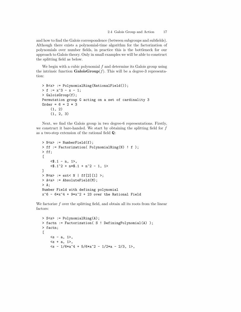
We begin with a cubic polynomial f and determine its Galois group usingthe intrinsic function GaloisGroup(f). This will be a degree-3 representa-tion:
> R<x> := PolynomialRing(RationalField());> f := x^3 - x - 1;> GaloisGroup(f);Permutation group G acting on a set of cardinality 3Order = 6 = 2 * 3
(1, 2)(1, 2, 3)
Next, we find the Galois group in two degree-6 representations. Firstly,we construct it bare-handed. We start by obtaining the splitting field for fas a two-step extension of the rational field Q:
> N<n> := NumberField(f);> ff := Factorization( PolynomialRing(N) ! f );> ff;[
<$.1 - n, 1>,<$.1^2 + n*$.1 + n^2 - 1, 1>
]> M<m> := ext< N | ff[2][1] >;> A<a> := AbsoluteField(M);> A;Number Field with defining polynomialx^6 - 6*x^4 + 9*x^2 + 23 over the Rational Field
We factorize f over the splitting field, and obtain all its roots from the linearfactors:
> S<s> := PolynomialRing(A);> factn := Factorization( S ! DefiningPolynomial(A) );> factn;[
<s - a, 1>,<s + a, 1>,<s - 1/6*a^4 + 5/6*a^2 - 1/2*a - 2/3, 1>,

18 2. Developed Examples
<s - 1/6*a^4 + 5/6*a^2 + 1/2*a - 2/3, 1>,<s + 1/6*a^4 - 5/6*a^2 - 1/2*a + 2/3, 1>,<s + 1/6*a^4 - 5/6*a^2 + 1/2*a + 2/3, 1>
]> C := [ -Coefficient(factr[1], 0) : factr in factn];> C;[
a,-a,1/6*a^4 - 5/6*a^2 + 1/2*a + 2/3,1/6*a^4 - 5/6*a^2 - 1/2*a + 2/3,-1/6*a^4 + 5/6*a^2 + 1/2*a - 2/3,-1/6*a^4 + 5/6*a^2 - 1/2*a - 2/3
]
Each of the roots is an algebraic conjugate of the primitive element a of thefield. The elements of the Galois group of A over Q are obtained by sendinga to one of its conjugates. Thus the action on A of such an element of theGalois group is determined by the polynomial (with rational coefficients)expressing the conjugate in a. These polynomials are stored in P below. We(again) determine the Galois group: by numbering the algebraic conjugatesci and finding all images of ci under a given Pj , we obtain the permutationassociated with Pj . The Galois group H consists of these permutations on 6letters.
> P := [ R ! Eltseq(x) : x in C];> P;[
x,-x,1/6*x^4 - 5/6*x^2 + 1/2*x + 2/3,1/6*x^4 - 5/6*x^2 - 1/2*x + 2/3,-1/6*x^4 + 5/6*x^2 + 1/2*x - 2/3,-1/6*x^4 + 5/6*x^2 - 1/2*x - 2/3
]> I := [ [ Index(C, Evaluate(p, c)) : p in P ] : c in C];> I;[
[ 1, 2, 3, 4, 5, 6 ],[ 2, 1, 4, 3, 6, 5 ],[ 3, 6, 1, 5, 4, 2 ],[ 4, 5, 2, 6, 3, 1 ],[ 5, 4, 6, 2, 1, 3 ],[ 6, 3, 5, 1, 2, 4 ]
]

2.4 Galois Group and Action 19
> H := sub< Sym(6) | I >;> H;Permutation group H acting on a set of cardinality 6
(1, 2)(3, 4)(5, 6)(1, 3)(2, 6)(4, 5)(1, 4, 6)(2, 5, 3)(1, 5)(2, 4)(3, 6)(1, 6, 4)(2, 3, 5)
Lastly, we find the Galois group G using the intrinsic function once more,but in terms of the degree-6 defining polynomial of the splitting field. It willbe conjugate to H: a simple renumbering of roots makes them equal. As wesee, we only need to cyclically permute three roots.
> G := GaloisGroup(DefiningPolynomial(A));> fl, el := IsConjugate(Sym(6), G, H);> fl, el;true (3, 4, 5)
Since we have the explicit action of the Galois group, we can now find thequadratic subfield of A corresponding to the subgroup K of H of order 3. Wecreate the sequence of automorphisms of A contained in K and see that thetrace of a3 generates the required quadratic field.
> S := Subgroups(H);> S;Conjugacy classes of subgroups------------------------------
[1] Order 1 Length 1Permutation group acting on a set of cardinality 6Order = 1
Id($)[2] Order 2 Length 3Permutation group acting on a set of cardinality 6
(1, 2)(3, 4)(5, 6)[3] Order 3 Length 1Permutation group acting on a set of cardinality 6
(1, 6, 4)(2, 3, 5)[4] Order 6 Length 1Permutation group acting on a set of cardinality 6
(1, 2)(3, 4)(5, 6)(1, 6, 4)(2, 3, 5)
> K := S[3]‘subgroup; // get subgroup from record S[3]

20 2. Developed Examples
> J := [ hom< A -> A | C[1^k] > : k in K ];> tra := &+[ h(C[1]^3) : h in J ];> tra, MinimalPolynomial(tra);3*a^3 - 9*ax^2 + 207> SquareFree(-207);-23 3
Therefore the quadratic subfield is Q(√−207) = Q(
√−23).

Part II
The Language


3. Basic Ideas
This chapter describes some elementary features of Magma. It explains howto produce output by evaluating expressions, how to assign a value to anidentifier, how to perform function calls, and how to handle common sub-expressions. In addition, it gives an overview of the operations on integers,rationals, reals, complex numbers, and Boolean values, and it shows how toinclude comments, recall previously printed values, and load input from afile.
3.1 Evaluating and Printing Expressions
An expression is a piece of Magma code which may be evaluated to return avalue. For example, the value of the expression 2+3 is 5, and the value of theexpression Denominator(2/7) is 7. A literal such as 87 is also an expression,with the obvious value.
The most direct way to determine the value of an expression is to printit, using a print-statement. The output is usually given on the computerscreen, or sent to a file if this has previously been arranged; it is not printedon paper. A simple print-statement consists of the word print, followed bythe expression whose value is to be printed, and finishing with a semicolon:
print expression;
More generally, the print-statement is able to evaluate and print severalexpressions, provided they are separated by commas:
print expression, expression, . . . , expression;
It should be noted that the token print may be omitted when workinginteractively. More precisely, print is mandatory only when used within func-tions, procedures and intrinsics. Otherwise its use is optional. In this book,since almost all of the examples are sections of an interactive run, print willusually be omitted.

24 3. Basic Ideas
This section illustrates the use of the print-statement, while explainingcertain common types of expression in Magma.
3.1.1 Arithmetic
The addition and subtraction operators in Magma are represented by the +and - symbols, as would be expected. As is the case in algebra, these opera-tors are left associative so that an expression consisting entirely of additionsand/or subtractions is evaluated in order from left to right. Parentheses maybe used to force a particular order of evaluation. For example:
> 15 - 5 + 3;13> 15 - (5 + 3);7
Since a print-statement may evaluate and print several expressions, thecalculations above could be written more succinctly as:
> 15 - 5 + 3, 15 - (5 + 3);13 7
Moreover, spaces around operators and commas are optional, so the state-ment above could also be typed as follows:
> 15-5+3,15-(5+3);13 7
However, appropriately placed spaces do tend to improve legibility.
The other standard arithmetic operations are equally straightforward, buttheir notation may be unfamiliar. The multiplication operator is an asterisk(*). Exponentiation is a caret (^) or an arrow (↑), depending upon the key-board being used. In the case of division, there are two kinds of operators: theslash (/) operator, which performs exact division; and div and mod, whichgive the quotient and remainder, respectively. The operators div and modare defined for pairs of elements of Euclidean Rings, whereas exact divisionis defined for pairs of elements of any ring provided that the divisor is a unitelement. As a special case, exact division when applied to the integers a andb constructs the element a
b of the rational field. For example, the followinglines illustrate the various division operators in the integer ring, the rationalfield, and the polynomial ring in x over the integer ring:
> 26 div 4, 26 mod 4;

3.1 Evaluating and Printing Expressions 25
6 2
> 26/4;13/2
> P<x> := PolynomialRing(IntegerRing());> (x^5 + 4) div (x^2 - 3*x + 1);x^3 + 3*x^2 + 8*x + 21> (x^5 + 4) mod (x^2 - 3*x + 1);55*x - 17
Using these operators, one can construct arbitrarily complicated arith-metic expressions. Magma’s operator precedence for the order of evaluationcorresponds to that used in arithmetic and algebra, but parentheses maybe used to override this or to clarify the expression for the human reader.Consider the arithmetic expression 7 × ((354 − 15)8 − 1892 × (53 div 2) +(24 mod 7)). It is evaluated and printed by the following statement:
> 7*((354-15)^8 - 1892*(53 div 2) + (24 mod 7));1220943664476136726244
3.1.2 Function Calls
Magma contains a very large number of standard pre-defined functions andprocedures, known as intrinsics. An intrinsic function is evaluated for specificvalues of its arguments by typing its name followed by the list of arguments,separated by commas and enclosed within parentheses. If the intrinsic doesnot have any arguments, the parentheses must still appear. The names ofintrinsics follow the rules for identifiers and almost all names for intrinsicsbegin with a capital letter. For example, the intrinsic function Factorial(n)returns n!, the factorial of an integer n. To evaluate and print 18!, the intrinsicFactorial is applied to the argument 18:
> Factorial(18);6402373705728000
The intrinsic function GCD(a, b) returns the greatest common divisor(gcd) of a and b, where a and b are elements of an Euclidean Ring. Thefollowing statement prints the gcd of 15130 and 3162:
> GCD(15130, 3162);34
The process of applying an intrinsic function to a particular set of valuesis often referred to as invoking or calling the function.

26 3. Basic Ideas
3.1.3 Printing Text
None of the Magma outputs above included any explanation of what theprinted values meant. It is often desirable to print some explanatory texttogether with a value. This may also be done with the print-statement. Thetext must be enclosed between double quotation marks ("), (note this is asingle character on the keyboard). For example:
> "Factorial of five is", Factorial(5);Factorial of five is 120
The object formed by enclosing characters in double quotation marks is calleda string. A detailed description of strings, including the formatting of outputusing the printf-statement, is given in Chapter 12.
3.2 Identifiers
3.2.1 Labelling Information
Suppose one is given several numbers, each of which has to be multiplied bysome fixed number. If the multiplier is easy to type, say one or two digits,then it is easy to calculate the products directly. However, if the multiplier islarge, this is tedious, and typing mistakes can easily occur. It would be mucheasier to type
m*5, m*73, m*48, m*636;
rather than
1492478*5, 1492478*73, 1492478*48, 1492478*636;
provided that Magma can be told that m stands for the multiplier.
The way to accomplish this is to type
> m := 1492478;
This instruction has the effect of storing the integer 1492478 in a ‘box’ inthe computer’s memory, and labelling it m. The technical term for a labelused to identify a piece of information stored in a computer is identifier orvariable, and the process of giving the identifier a value is called assignment.

3.2 Identifiers 27
Once the identifier m has been assigned the value 1492478, Magma willsubstitute this value wherever m appears in an expression. If m is later as-signed a different value, this new value will be substituted in subsequentexpressions involving m. A print-statement will give the current value of m:
> m;1492478
and the following line solves the initial problem:
> m*5, m*73, m*48, m*636;7462390 108950894 71638944 949216008
An identifier may have as its value, any object definable in Magma: aninteger, a group element, a set, a rational number, a string or a vector space.The main role of identifiers, other than for purposes of abbreviation, is thatthey allow the construction of more general program statements than thosethat can be formed using constants alone. Because of their utility, it is usualfor many identifiers to be used in a large Magma program.
Identifier names are not restricted to a single letter, such as m. In fact,it is a good idea to choose longer and meaningful names, so as to remind areader (including the author!) of the value named by that identifier. Someuseful names might be len (for ‘length’), product , lowlimit or uplimit . Anidentifier may be constructed from letters, digits or the underscore character_, provided that it does not commence with a digit. Thus, side3 and angle Aare examples of legal identifier names, while 3n is not legal. There are fourtraps to avoid in choosing identifiers:
– A Magma reserved word such as print or mod may not be used as anidentifier. See p. 299 for a list of the reserved words.
– Although it is possible assign a value to an identifier that is the name of anintrinsic function (e.g., Factorial), this is very unwise since the intrinsicwill no longer be available. It may be retrieved by applying the delete-statement to the intrinsic identifier which has been redefined.
– Magma distinguishes between upper and lower case letters. For example,rc, RC , rC and Rc are distinct identifiers.
– The identifier name _ has a special use as the throwaway identifier, so itmay not be used as an ordinary identifier name. See p. 32 of this chapterfor details.

28 3. Basic Ideas
3.2.2 Showing All Identifiers and Their Values
The intrinsic procedure ShowIdentifiers() prints a list of all the identifiersthat are currently assigned. A similar procedure, ShowValues(), prints allthese identifiers together with their values.
In the example below, it should be assumed that no assignments havebeen made prior to the beginning of the example:
> Z := IntegerRing();> d := 7;> len := 82/35;> ShowIdentifiers();Z d len> ShowValues();Z:
Integer Ring
d:7
len:82/35
3.2.3 Deletion and Unassigned Identifiers
If a Magma session has involved the creation of very large objects, or largenumbers of smaller objects, process space (i.e., workspace) may be exhausted.Memory may be freed using the delete-statement to remove unwanted data:
delete identifier, identifier, . . . , identifier;
This statement deletes the current values of all the listed identifiers, so thatthey revert to the status of identifiers that have not been assigned. The formervalues of those identifiers will be lost irrevocably from Magma’s memory.
The unary operator assigned allows the user to test whether an identifieris currently assigned a value. It returns true or false. For example:
> zxcv := 47;> assigned zxcv;true> delete zxcv;> assigned zxcv;false

3.3 Assignment 29
3.3 Assignment
3.3.1 The Simple Assignment Statement
Various examples of assigning a value to an identifier have appeared above.The general form of an simple assignment statement is
identifier := expression;
where the expression involves identifiers and/or constants. When Magmaencounters this statement, it evaluates the expression on the right hand side,stores the resulting value, and associates the identifier with that value. If anerror occurs during the evaluation of the expression, the identifier will not beassigned a value.
For example, suppose that the dimensions of a solid box are L = 14,B = 12 and H = 6, and the volume of the box has to be stored in V . Firstly,the identifiers L, B and H should be assigned:
> L := 14;> B := 12;> H := 6;
Note that as it is legal to have several statements on the same line, theassignment of L, B and H above could have been written on a single line:
> L := 14; B := 12; H := 6;
Now that L, B and H have their values, V may be calculated in terms ofthese identifiers:
> V := L * B * H;
Then V may be accessed on demand.
> V;1008
> "Volume is", V, "cubic units.";Volume is 1008 cubic units.
and it can also be used to calculate other quantities such as the mass of thebox, given that the box’s density is 100 units:
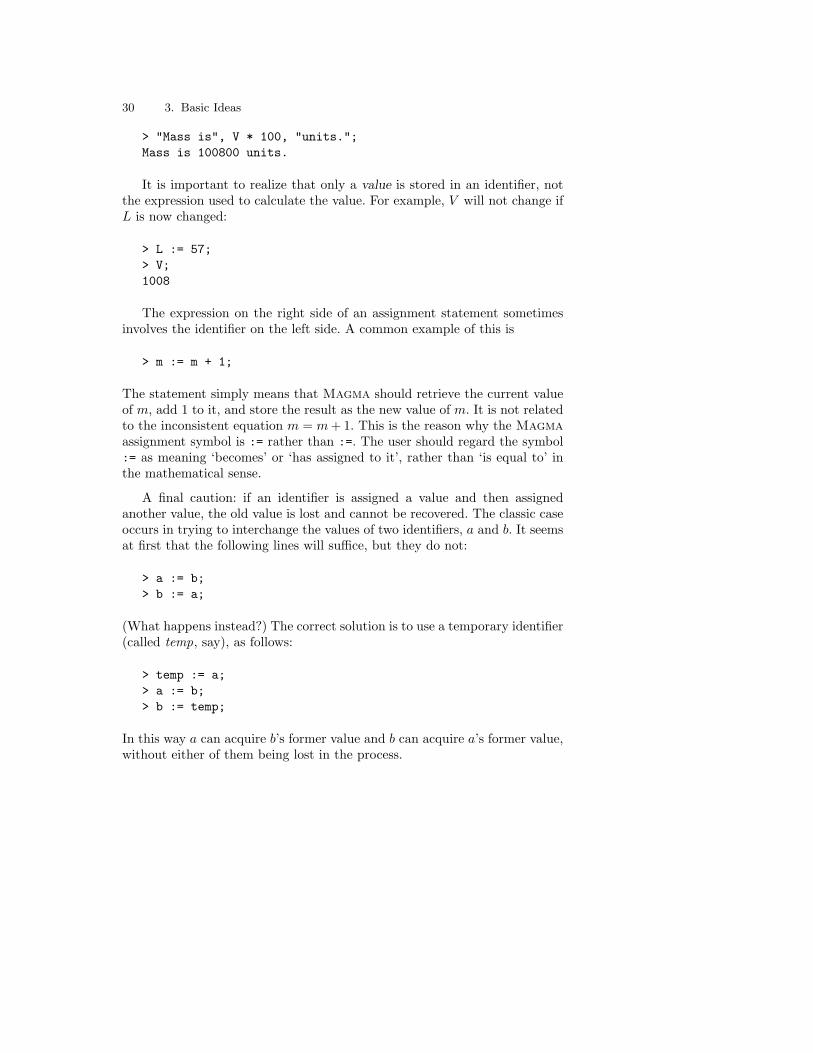
30 3. Basic Ideas
> "Mass is", V * 100, "units.";Mass is 100800 units.
It is important to realize that only a value is stored in an identifier, notthe expression used to calculate the value. For example, V will not change ifL is now changed:
> L := 57;> V;1008
The expression on the right side of an assignment statement sometimesinvolves the identifier on the left side. A common example of this is
> m := m + 1;
The statement simply means that Magma should retrieve the current valueof m, add 1 to it, and store the result as the new value of m. It is not relatedto the inconsistent equation m = m + 1. This is the reason why the Magmaassignment symbol is := rather than :=. The user should regard the symbol:= as meaning ‘becomes’ or ‘has assigned to it’, rather than ‘is equal to’ inthe mathematical sense.
A final caution: if an identifier is assigned a value and then assignedanother value, the old value is lost and cannot be recovered. The classic caseoccurs in trying to interchange the values of two identifiers, a and b. It seemsat first that the following lines will suffice, but they do not:
> a := b;> b := a;
(What happens instead?) The correct solution is to use a temporary identifier(called temp, say), as follows:
> temp := a;> a := b;> b := temp;
In this way a can acquire b’s former value and b can acquire a’s former value,without either of them being lost in the process.

3.3 Assignment 31
3.3.2 The Mutation Assignment Statement
There is an alternative form of assignment statement available for making asimple change to an existing identifier that involves its former value. Supposethat the following assignment has been made:
> d := 7;
and then d has to be multiplied by 53. Instead of typing
> d := d * 53;
the user can type
> d *:= 53;
This is known as a mutation assignment because it mutates, or changes, theold value of the identifier. Its general form is
identifier := expression;
where is the operator, and it has the same end result as
identifier := identifier expression;
Apart from being more compact than the standard assignment, a mutationassignment is often more efficient since Magma can operate directly on theidentifier’s value without first having to make a copy of it.
3.3.3 Multi-Valued Expressions and the Multiple AssignmentStatement
Certain classes of expression in Magma may return multiple values. In par-ticular. functions may return several values, and constructors, such as suband quo, (see Chapter 4), return both a structure and an associated mapping.Such an expression will be termed a multi-valued expression. The manner inwhich these multiple values are handled depends upon the context in whichthe expression appears. There are four cases:
– The expression forms the right-hand side of an assignment statement inwhich exactly one identifier appears on the left-hand side. In this case,only the first value will be computed.

32 3. Basic Ideas
– The expression forms the right-hand side of an assignment statement inwhich more than one identifier appears on the left-hand side (includingthrowaway identifiers). All the values are created and the designated onesare assigned.
– The expression is embedded as part of a larger expression. In this case onlythe first value (the principal value) is computed and used when evaluatingthe outer expression.
– The expression is a term in a print list. Here the principal value is alwaysprinted while the remaining values may or may not be printed dependingupon circumstances.
To access the values returned by a multi-valued assignment a multipleassignment statement is provided. It has the syntax:
identifier, . . . , identifier := multiple-value expression;
For example, the function Quotrem(a, b) returns the values of both a div band a mod b:
> q, r := Quotrem(26, 4);> q, r;6 2> 4*q + r;26
If such an expression forms part of a larger expression, then only theprincipal value (the first return value) will be used:
> 5 * Quotrem(100, 13);35
In the case of some multiple return value expressions, the print-statementwill display all the return values. Whether this happens or not is decided on acase-by-case basis; as a guide, all the values will be printed if they are cheapto compute, generate little output and convey useful information.
The number m of identifiers on the left of the multiple assignment state-ment must be less than or equal to the total number n of return values. Ifm is strictly less than n, then only the first to the mth return values of theexpression will be returned and assigned. The special _ character (known asthe throwaway identifier) may be used in the identifier list to discard thecorresponding return value:
> qq := Quotrem(100, 13);
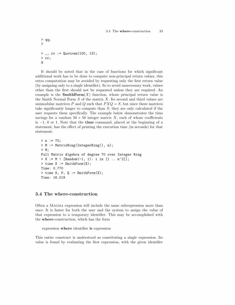
3.4 The where-construction 33
> qq;7
> _, rr := Quotrem(100, 13);> rr;9
It should be noted that in the case of functions for which significantadditional work has to be done to compute non-principal return values, thisextra computation may be avoided by requesting only the first return value(by assigning only to a single identifier). So to avoid unnecessary work, valuesother than the first should not be requested unless they are required. Anexample is the SmithForm(X) function, whose principal return value isthe Smith Normal Form S of the matrix X. Its second and third values areunimodular matrices P and Q such that PXQ = S, but since these matricestake significantly longer to compute than S, they are only calculated if theuser requests them specifically. The example below demonstrates the timesavings for a random 50 × 50 integer matrix X, each of whose coefficientsis −1, 0 or 1. Note that the time command, placed at the beginning of astatement, has the effect of printing the execution time (in seconds) for thatstatement:
> n := 70;> M := MatrixRing(IntegerRing(), n);> M;Full Matrix Algebra of degree 70 over Integer Ring> X := M ! [Random(-1, 1): i in [1 .. n^2]];> time S := SmithForm(X);Time: 0.770> time S, P, Q := SmithForm(X);Time: 16.019
3.4 The where-construction
Often a Magma expression will include the same subexpression more thanonce. It is faster for both the user and the system to assign the value ofthat expression to a temporary identifier. This may be accomplished withthe where-construction, which has the form
expression where identifier is expression
This entire construct is understood as constituting a single expression. Itsvalue is found by evaluating the first expression, with the given identifier

34 3. Basic Ideas
taking as its value, the value of the second expression. (For convenience, theassignment symbol := may be used instead of is.)
For example, let P be the polynomial ring in x over the integers:
> P<x> := PolynomialRing(IntegerRing());
Suppose that the user wants to create f = d(d+1)(d2+5) where d is x5−4x3+17. Without using the where-construction, there are two methods. Firstly,the user could type the expression for d into every part of the expression for fin which it appears. This would involve excessive typing, and the expressionfor d may have to be evaluated several times by the system. Secondly, theuser could assign x5 − 4x3 + 17 to the identifier d, and then create f :
> d := x^5 - 4*x^3 + 17;> f := d*(d + 1)*(d^2 + 5);> f;x^20 - 16*x^18 + 96*x^16 + 69*x^15 - 256*x^14 - 828*x^13 +
256*x^12 + 3312*x^11 + 1790*x^10 - 4416*x^9 - 14320*x^8+ 28640*x^6 + 20694*x^5 - 82776*x^3 + 89964
This approach is preferable to the first, but is not ideal for two reasons: thevalue of d is not otherwise required; and if d already had a value, then thisvalue would be lost. The where-construction affords a superior solution:
> f := d*(d + 1)*(d^2 + 5) where d is x^5 - 4*x^3 + 17;> f;x^20 - 16*x^18 + 96*x^16 + 69*x^15 - 256*x^14 - 828*x^13 +
256*x^12 + 3312*x^11 + 1790*x^10 - 4416*x^9 - 14320*x^8+ 28640*x^6 + 20694*x^5 - 82776*x^3 + 89964
The scope of the identifier in the where-construction is limited to thatconstruction, so it does not affect an identifier of the same name outside it.Consider the following:
> d := 1000;> f := d*(d + 1)*(d^2 + 5) where d is x^5 - 4*x^3 + 17;> d;1000
Notice that d has kept its old value. If d had not been assigned, then afterthe where-construction it would have remained unassigned.
Several where-constructions may be used in succession. For example,each of the following statements assign the same value to m:

3.5 Integers, Rationals, Reals, and Complex Numbers 35
> m := (n-2)*Factorial(n) where n is k^2-3*k+1 where k is 4;
> m := (n-2)*Factorial(n) where n is 4^2-3*4+1;
> m := (5-2)*Factorial(5);
If an expression involves successive where-clauses, they associate to the left.As an example, compare the following three expressions. The first two eval-uate to give the same result, but the third yields a different value:
> x := 1; y := 2;> x + y where x is 5 where y is 7;12> (x + y where x is 5) where y is 7;12> x + y where x is (5 where y is 7);7
In the case of a comma-separated expression list, the effect of a where-clause will extend left across the commas, but not right. Such expression listsare used as the arguments of a function or procedure, in print-statements,and in other statements not yet introduced (e.g., return and error). Inthe following example, notice that the first two expressions in the print-statement are evaluated using the values for x and y given in the where-constructions, but the other expression is evaluated using the external valuesx = 1 and y = 2:
> x := 1; y := 2;> x-y, x+y where x is 5 where y is 7, x*y;-2 12 2
3.5 Integers, Rationals, Reals, and Complex Numbers
Arithmetic with integers has already been demonstrated. There are no sizerestrictions on integers in the case of arithmetic operations (except for expo-nentiation, in which the absolute value of the exponent must be less than aconstant, dependent upon the word-length of the computer):
> n := 9817855152457389762535312;> n * (n+1);96390279794634115977367954214982109558227809472656

36 3. Basic Ideas
Rational numbers in Magma are expressed in fractional form, and realnumbers in decimal form:
> halfA := 1/2;> halfB := 0.5;
A rational number such as 20 47 may be entered as either 20 + 4/7 or 144/7.
A real number having very large or very small magnitude may be enteredin scientific notation, using e to denote the base 10. For example, the inputsyntax for 5.2× 10⁻¹⁶ is:
> smallnum := 5.2e-16;
A complex number is best created as an expression involving two real numbersand i =
√−1, where i is created using the ComplexField() function:
> C<i> := ComplexField();> z := 2.6 + 3.7*i;
Rational arithmetic in Magma is performed to arbitrary precision, sinceit is based internally on integer arithmetic. Real/complex arithmetic is per-formed to free precision or to a fixed precision, depending on the setting ofthe default real field; see Chapter 26.
Magma can usually cope easily with an expression involving both aninteger and a rational, real or complex number, by coercing the integer intothe appropriate field. However, for some applications Magma must be toldexplicitly that an integer is to be considered as a real, rational or complexnumber. The easiest way of doing this to write it as such, as shown below:
> rat37 := 37/1;> real37 := 37.0;> cmplx37 := 37.0 + 0*i;
These numbers will be deemed by Magma to be equal to the integer 37, butthe structure to which they belong (their parent magma) will be the rational,real or complex field rather than the integer ring:
> Parent(rat37), Parent(real37), Parent(cmplx37);Rational FieldReal FieldComplex Field
An alternative way to construct rat37 , real37 and cmplx37 is to coerce themexplicitly into the required structure, using the ! operator:

3.6 Booleans 37
> rat37 := RationalField() ! 37;> real37 := RealField() ! 37;> cmplx37 := C ! 37;
This method produces approximately the same results as above, but is slightlypreferable in the real and complex case since the coerced integers will haveinfinite precision.
Integers, rationals, reals and complex numbers share most of the commonarithmetic operators, but, in addition, each has its own special functions. Forexample:
> Numerator(r), Denominator(r) where r is 6/4;3 2> Sin(4.6);-0.993691003633464456138104659913700464630> Round(x), Truncate(x) where x is 3.7;4 3> Sqrt(-3); // square root1.73205080756887729352744634149*i> ComplexToPolar(3 + 4*i); // modulus and argument5.00000000000000000000000000000.92729521800161223242851246291
Integers and rationals are discussed in more detail in Chapter 20, and realand complex numbers in Chapter 26.
3.6 Booleans
Table 3.1. Relational operators
Operator Maths Usage Meaning
eq = x eq y true iff x is equal to y
ne 6= x ne y true iff x is not equal to y
lt < x lt y true iff x is less than y
le ≤ x le y true iff x is less than or equal to y
gt > x gt y true iff x is greater than y
ge ≥ x ge y true iff x is greater than or equal to y
One of the most basic structures available in Magma is the Booleanstructure, so named after the logician George Boole. The Boolean structure

38 3. Basic Ideas
contains two values: true and false. Boolean values are used to describe atwo-state system, such as yes/no, on/off, or true/false.
There are several operators that return a Boolean value. The relationaloperators test if two quantities are related in a certain way and they thenreturn an answer of true or false. For example, x eq y returns true ifand only if x equals y. The principal relational operators are described inTable 3.1. In this table, and in all other tables listing functions and operatorsreturning Booleans, it should be noted that ‘iff’ is an abbreviation for ‘if andonly if’. Some illustrations are:
> 3+4 eq 7;true> 100 eq 1000-0;false> 2/3 lt 3/4;true
Table 3.2. Boolean operators
Operator Usage Meaning
not not a true iff a is false
and a and b true iff both a and b are true
or a or b true iff at least one of a and b are true
xor a xor b true iff exactly one of a and b is true
Table 3.2 lists the Boolean operators. They operate on Boolean valuesand return Boolean results. For example:
> (3+4 gt -5) and (2 le 3);true
The meanings of the Boolean operators correspond fairly closely to the ordi-nary meanings of the corresponding words, except that that or is inclusive(true if and only if one or both of a and b are true), whereas xor is exclusive(true if one of a and b is true but not if both are true). In other words, or isin accordance with the use of ‘or’ in ‘This seat is reserved for aged or disabledpersons’ and xor corresponds to ‘or’ in ‘Would you like coffee or tea?’.
Expressions involving the operators and and or are evaluated using con-ditional evaluation, as distinct from Magma’s usual call-by-value evaluation.Conditional evaluation of an expression has the effect that arguments areevaluated only as required, from left to right, stopping as soon as the return
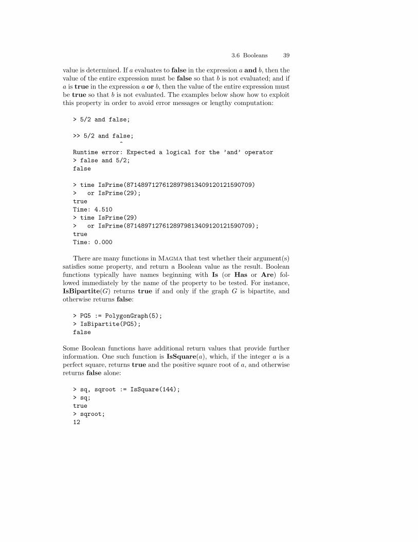
3.6 Booleans 39
value is determined. If a evaluates to false in the expression a and b, then thevalue of the entire expression must be false so that b is not evaluated; and ifa is true in the expression a or b, then the value of the entire expression mustbe true so that b is not evaluated. The examples below show how to exploitthis property in order to avoid error messages or lengthy computation:
> 5/2 and false;
>> 5/2 and false;^
Runtime error: Expected a logical for the ’and’ operator> false and 5/2;false
> time IsPrime(87148971276128979813409120121590709)> or IsPrime(29);trueTime: 4.510> time IsPrime(29)> or IsPrime(87148971276128979813409120121590709);trueTime: 0.000
There are many functions in Magma that test whether their argument(s)satisfies some property, and return a Boolean value as the result. Booleanfunctions typically have names beginning with Is (or Has or Are) fol-lowed immediately by the name of the property to be tested. For instance,IsBipartite(G) returns true if and only if the graph G is bipartite, andotherwise returns false:
> PG5 := PolygonGraph(5);> IsBipartite(PG5);false
Some Boolean functions have additional return values that provide furtherinformation. One such function is IsSquare(a), which, if the integer a is aperfect square, returns true and the positive square root of a, and otherwisereturns false alone:
> sq, sqroot := IsSquare(144);> sq;true> sqroot;12

40 3. Basic Ideas
> sq, sqroot := IsSquare(143);> sq;false> assigned sqroot;false
3.7 Comments
It is standard practice to include comments in a computer program to describeits purpose and its internal logic. Such remarks are ignored by the computer.
A comment is placed between the /* and */ symbols; Magma will ig-nore anything between these symbols, and the symbols themselves. Note thatcomments may not be nested. Alternatively, any text following the symbols// on a line will be ignored (treated as a comment).
The following example is rather artificial because of its shortness, butcomments may also be found in other examples in this book:
> /*> * Find the volume of a box,> * given its length, breadth, and height.> */> // assign the dimensions> L := 14; // length> B := 12; // breadth> H := 6; // height> // compute the volume> V := L * B * H;
3.8 Recalling Previously Printed Values
It frequently occurs that a user requires a value printed by an earlier print-statement, where the value has not been assigned to an identifier. Since itwould be inefficient to recompute the value, Magma provides a facility forrecalling values that have been obtained by evaluating expression lists inprint-statements.
The list of values displayed by the most recent print-statement corre-sponds to $1, the list of values in the next most recent print-statementcorresponds to $2, and so on. The number after the dollar sign must be aliteral integer, not a general expression evaluating to an integer. For example:

3.8 Recalling Previously Printed Values 41
> z := 15;> 3 * z;45> y := 13;> $1;45> z * y + 1;196> $1 - $2; // i.e., 196 - 45151
If several values were previously printed in a single statement, then thedollar construct will return all of them exactly as if it were a multi-valuedexpression, so the values may be assigned using the multiple assignment state-ment. For example:
> 12 * 9, 4 * 8;108 32> a, b := $1;> a;108> b;32
> Quotrem(5000, 183);27 59> c, d := $1;> c;27> d;59
The previous values (or more accurately, previous value lists) are storedin the previous value buffer. The maximum number of entries in this bufferis returned by the function GetPreviousSize(). The default value is 3, butit may be changed to any small non-negative integer n by means of the pro-cedure SetPreviousSize(n). Note that SetPreviousSize simply specifies anew buffer size; increasing the maximum will not restore very old values, asdemonstrated below:
> Factorial(4);24> Factorial(5);120> Factorial(6);

42 3. Basic Ideas
720> Factorial(7);5040> $4;
>> $4;^
Runtime error: Previous value number (4) should be in the range [1 .. 3]> SetPreviousSize(6);> Factorial(8);40320> $5;
>> $5;^
Runtime error: Previous value number (5) should be in the range [1 .. 4]
As will be evident from the end of the preceding example, printing a previ-ous value changes the previous value buffer, just as is the case with any otherprint-statement. However, the procedure ShowPrevious allows the user toinspect the values in the buffer without affecting the contents of the buffer.ShowPrevious(i) displays the value $i, and ShowPrevious() displays thewhole buffer. The next example should be understood as a continuation ofthe one before:
> ShowPrevious(3);$3: 720> ShowPrevious();$4: 120$3: 720$2: 5040$1: 40320> $3;720
The procedure ClearPrevious() deletes all values stored in the previousvalue buffer.
3.9 Loading Input from a File
Short bodies of code may easily be typed directly into Magma. For longerprograms, it is usually more efficient to create blocks of code as text filesexternal to Magma. The creation and editing of such files is performed using

3.9 Loading Input from a File 43
whatever software the computer offers, and does not involve Magma. Afterthe file has been created, its contents may be loaded into Magma by typing:
load "filename";
where ‘filename’ is the name of the file. Magma will execute each line of thefile just as if it had been typed directly intoMagma. The load-statementmust appear at the top level, that is, it may not be included within any otherstatement.
If the file does not reside in the current directory then the directory mustbe specified as well. Alternatively, the directory may be included in the en-vironment variable MAGMA_PATH. See p. 278.
For example, suppose a file, m11pol, has been created containing thefollowing statements:
Q := RationalField();R<x> := PolynomialRing(Q);f := x^11 - x^10 - 121*x^9 + 65*x^8 + 5345*x^7 -
481*x^6 - 96739*x^5 - 23689*x^4 + 413690*x^3 -493810*x^2 + 26910*x - 856170;
print "The following polynomial f of degree 11 is defined:";print f;
Now, from within Magma, the user may load this file as many times asdesired. Each time it is loaded, the statements in it are executed:
> load "m11pol";Loading "m11pol"The following polynomial f of degree 11 is defined:x^11 - x^10 - 121*x^9 + 65*x^8 + 5345*x^7 - 481*x^6 -
96739*x^5 - 23689*x^4 + 413690*x^3 - 493810*x^2 +26910*x - 856170
> G := GaloisGroup(f);> G;Permutation group G acting on a set of cardinality 11
(1, 4, 6, 8, 10)(2, 7, 9, 11, 5)(1, 9, 10)(3, 7, 5)(4, 6, 11)(1, 6, 5, 3, 10)(2, 4, 9, 7, 11)
> CompositionFactors(G);G| M111

44 3. Basic Ideas
Not only can the user’s own files be loaded into Magma, but also manyother files provided with the Magma system. There are two main kinds ofthese files: library or database definitions of commonly-used algebraic struc-tures and functions, and certain labelled examples from this book and theHandbook. When examples from the books are loaded, (most of) the contentsof the file containing the example are echoed to the terminal so that they canbe seen. This does not necessarily happen when a file is loaded, but happensfor these examples because the function SetEchoInput is being used. Theinterested reader is advised to look at some of the files and read p. 280 tounderstand how it works.
Magma also provides a package mechanism, which provides for the auto-loading of files. Given a file containing the user’s definitions of functions andprocedures in a special syntax, it is able to incorporate these routines intoMagma as user intrinsics (as distinct from system intrinsics). Chapter 10explains the use of packages.

4. Algebraic Structures
Structures are the weapons of the mathematician.
See Scientific American May 1957Nicholas Bourbaki
With almost no exceptions, any object x definable in the Magma lan-guage is viewed as an element of some algebraic structure A. The propertiesof A define the operations that may be performed on x. As a general rule,the structure A must be defined before its element x (although there areexceptions). It is therefore very important for the reader to understand howthe concept of an algebraic structure is realised in Magma together with themechanisms provided for constructing them.
Many different types of algebraic structures may be constructed in Magma,including polynomial rings, number fields, vector spaces, modules, matrix al-gebras, and finitely-presented groups. However, this diverse range of struc-tures share certain common conventions concerning operators for arithmetic,creating substructures and quotient structures, and testing membership.
This chapter provides an overview of the Magma philosophy concerningalgebraic structures and their elements, and introduces the principal syntacticconstructs for their creation and manipulation. It should be skimmed on firstreading, and referred to later as needed.
4.1 Magmas, Categories and Varieties
The organization and interrelationship of algebraic structures in Magma isbased on ideas from Universal Algebra and Category Theory. Every objectthat is definable in Magma is regarded as belonging to a set M (usually thecarrier set associated with an algebraic structure). Such sets are referred to as

46 4. Algebraic Structures
magmas; the term being a generalization of the Bourbaki definition ([Bou70],ch. 1, p. 1) of a magma as a set with one or more laws of composition.1
The magma to which an object belongs is called its parent magma. Givenan object x, the function Parent(x) returns its parent. For example, theparent of the real number 62.7 is the real field:
> Parent(62.7);Real Field
Since every object that can be created in Magma is ultimately defined interms of one or more magmas, it is necessary to be able to refer to anymagma. For example, a function that creates a polynomial ring P in theindeterminate t over some ring, will take the coefficient ring as its argument.In the example below, the construction of the magma comprising the ring ofunivariate polynomials over Q is created using the function RationalField()which defines the magma Q.
> Q := RationalField();> P<t> := PolynomialRing(Q);> P;Univariate Polynomial Algebra in t over Rational Field
> Parent(t^2 + 5*t + 6);Univariate Polynomial Algebra in t over Rational Field> Parent(t^2 + 5*t + 6) eq P;true
The output shows that the parent of t2 + 5t + 6 is P .
Similar magmas are organized into classes known as categories. More pre-cisely, a category is a class of magmas satisfying a particular set of axiomsand sharing a common representation. The category to which a magma be-longs determines the set of operations that may be applied to its elements.For example, if x and y are elements of a permutation group G, then thisparent magma G belongs to the category of permutation groups, GrpPerm.It is from the membership of their parent in this category that the processorknows that x*y is defined but x + y is not; that is, there is a multiplicationalgorithm that operates on a pair of permutation group elements, but thereis no addition algorithm.
The function Category(M), or equivalently Type(M), returns the cat-egory of M . Continuing the previous example, the following output showsthat P belongs to RngUPol, the category of rings of univariate polynomialsover any ring and in any indeterminate:1 ‘Un ensemble muni d’une loi de composition est appele un magma.’

4.1 Magmas, Categories and Varieties 47
> Category(P);RngUPol
The procedure ListCategories() lists the names of all the categories inMagma:
> ListCategories();Alg GrpMatElt PowSetEnumAlgChtr GrpPC PowSetFormalAlgChtrElt GrpPCElt PowSetIndxAlgCon GrpPCStdPresProc PowSetMulti
...
For most elementary purposes it is not necessary to know the precise namesMagma uses for the categories. They are required for a few intrinsics; anexample is DihedralGroup(C, n), which takes a category C as its first ar-gument so that Magma knows whether to construct the dihedral group oforder 2n as a permutation group, a finitely-presented group, or so on. SeeSection 29.1.3 for details. Category names are also required for the creation ofuser intrinsics, as described in Chapter 10, in order to specify the categoriesof arguments and return values.
Note carefully that the possession of some mathematical property by aparticular magma in a category does not imply that this property will be au-tomatically exploited by the Magma system. In general, unless the propertyis common to all magmas belonging to the category, operations dependingupon it will not be defined. For example, if a quotient ring of a univariatepolynomial ring over Q (category RngMPolRes) happens to be a field, thenoperations defined exclusively for the category of number fields (FldNum)are not automatically available. In order to access such operations, the fieldmust be explicitly created as a member of FldNum. In summary, the oper-ations available for a particular magma are defined by the category in whichit is created.
Finally, a collection of categories whose magmas satisfy a common setof axioms forms a variety. For example, GrpAb (finitely-generated abeliangroups), GrpMat (matrix groups) and GrpFP (finitely-presented groups)are some of the categories belonging to the variety of groups. While a user sel-dom needs to be aware of the existence of varieties, the concept is used by theMagma implementers to write code that is independent of the representation(as determined by the category).
In some cases, Magma provides functors for moving from one categoryto another or from one variety to another. For instance, AbelianGroup(G)returns the abelian group (in category GrpAb) corresponding to the abelianmatrix group G (in category GrpMat), and VectorSpace(A) returns the

48 4. Algebraic Structures
vector space (in ModTupRng) underlying a finite dimensional associativealgebra A (in AlgCon).
4.2 Creation of Magmas
The creation of a magma M in the Magma system requires, in principle, twosteps:
1. The definition of an appropriate ‘free’ magma F ;
2. The construction of the desired magma M from F by applying a sequenceof constructions that create substructures, normal closures, ideals, quo-tient structures and extensions until M is reached.
For each category possessing free magmas, a function is provided that con-structs a free magma F . The derivation of a magma from an existing magmavia generic operations is accomplished by constructors of the form
constructor< magma | details of construction >
The principal constructor names, appearing to the left of the < symbol, aresub, ncl, ideal, quo and ext, designating submagmas, normal closures (inthe case of groups), ideals, quotients and extensions.
If a magma with r generators is assigned to an identifier M , then M .idenotes the ith generator, where 1 ≤ i ≤ r. However, it is customary to givenames to the generators of M at the same time as M is assigned. This maybe accomplished by means of a generator assignment statement, with thefollowing syntax:
M< x1, . . . , xr > := expression defining M ;
(Here the x1, . . . , xr must obey the usual rules for identifier names.) Theprincipal effect of this statement is to assign M in the usual way. Its auxil-iary effect is to create the identifiers x1, . . . , xr and assign to them the valuesof the generators. As a result, either xi or M .i may be used in an inputexpression, to denote the ith generator of M . The third effect of the state-ment operates only for magmas such as free or finitely-presented structures(including polynomial rings), whose elements are printed explicitly in termsof generators: the printname (output form) of each generator is changed fromM .i to xi, so as to increase the legibility of the output.
For example, consider the polynomial ring R over the rational field inthree indeterminates. The following statement constructs R, assigns its inde-

4.3 Automatically-Created Magmas 49
terminates to the identifiers x, y, z, and indicates that the indeterminates areto be printed as x, y, z:
> R<x,y,z> := PolynomialRing(RationalField(), 3);> R;Polynomial ring of rank 3 over Rational FieldLexicographical OrderVariables: x, y, z> x + 2*y*z;x + 2*y*z
In the following sections, the creation of magmas and their elements willbe explained more fully.
4.3 Automatically-Created Magmas
Five magmas are created automatically when a Magma session begins. Theyare the integers, the rationals, the free real field (with default precision at-tribute 28), the Booleans, and the monoid of character strings. Because thesemagmas are automatically created, it is unnecessary when referring to theirelements to declare the parent explicitly. The Magma input representation ofelements belonging to such magmas allows the language processor to deducethe appropriate parent magma. For instance, given the statements
> three := 3;> NumberTheory := "queen of mathematics";
then Magma can deduce that the parents of the objects are the integer ringand the string monoid, respectively:
> Parent(three), Parent(NumberTheory);Integer RingString structure
Table 4.1 lists functions each of which returns, as its value, one of the fiveautomatically-created magmas. Although these magmas are defined whenthe system starts up, and therefore do not require explicit ‘creation’, it issometimes necessary to refer to them when defining magmas inductively, asillustrated above in the example of the polynomial algebra over the rationals.Moreover, if several magmas are being defined in terms of the same magma,it is advisable to assign the magma to an identifier so that the function doesnot have to be called repeatedly:

50 4. Algebraic Structures
Table 4.1. Functions for the automatically-created magmas
Magma Meaning
IntegerRing() The ring of integers
RationalField() The field of rational numbers
RealField() The free field of real numbers (default precision 28)
Strings() The string monoid (over the ASCII character set)
Booleans() The Boolean structure, containing true and false
> Q := RationalField();> Q;Rational Field
Each of these five magmas has its own category, a category to which noother magmas belong. (An exception is the integer ring category, to whichideals of integer rings also belong for the sake of efficiency; see Section ??.)These categories are RngInt, FldRat, FldPr, MonStg, and Bool. Detailsof these categories are given in Chapter 20 for the integers and rationals,Chapter 26 for the reals, Section 3.6 for the Booleans, and Chapter 12 forthe strings.
4.4 Creating a Free Magma
When creating a magma M , the general strategy is to first create the ap-propriate free magma F and then create the desired submagma or quotientmagma M in terms of it. This section explains what is meant in Magma bythe concept free magma, and illustrates the construction of such magmas. Todefine other magmas the user must also to know how to define elements ofmagmas; this is discussed in the following section.
Given a variety V (e.g., groups, rings), the free magma F in V with n gen-erators may be informally described as the unique algebraic structure whoseelements are all possible finite arithmetic combinations of the n generators.Here the meaning of ‘arithmetic combination’ depends on V , but will typ-ically involve sums, products, and/or the taking of inverses. (This informalnotion of ‘free magma’ corresponds to the concept of a term algebra.)
For example, the free group FG3 on three generators a, b, c is the groupconsisting of the set of equivalence classes of finite products of a, b, c, a−1, b−1
and c−1. It may be created in Magma as follows:
> FG3<a,b,c> := FreeGroup(3);

4.5 Creating and Operating on Elements of a Magma 51
> FG3;Finitely presented group FG3 on 3 generators (free)
Magma uses the concept of free magma in a looser sense as well, todescribe the largest possible magma of a given category with the given pa-rameters. Such magmas are often called generic or full. For example, in thegroup category of permutation groups, the free magma for each degree nis Sym(n), the symmetric group of degree n (i.e., the group consisting ofall permutations of n elements). Similarly, in the module category of vectorspaces, the free magma for each field K and dimension n is the vector spaceK(n), that is, the space of all n–dimensional vectors whose entries are ele-ments of K. For instance, the symmetric group of degree 6 may be created asshown below, using the SymmetricGroup function (commonly abbreviatedto Sym):
> s6 := Sym(6);> s6;Symmetric group s6 acting on a set of cardinality 6Order = 720 = 2^4 * 3^2 * 5
and the following lines create the finite field with 27 elements (assigning itsgenerating element to w) and then the full four-dimensional vector space withcoefficients taken from this field:
> GF27<w> := GaloisField(27);> GF27;GF(3^3)> VS4 := VectorSpace(GF27, 4);> VS4;Full Vector space of degree 4 over GF(3^3)
4.5 Creating and Operating on Elements of a Magma
Objects in Magma may arise as the values of many kinds of expressions,including function calls. However, there are two basic ways to create a newobject as an element of a magma M :
– As a literal element, using an elt-constructor, sequence-coercion, or someother syntax for literal elements that is unique to the category of M ;
– Arithmetically, from generators or previously assigned elements of M .

52 4. Algebraic Structures
This section examines the creation of literal elements, followed by an ex-planation of how to use arithmetic operators to build elements from otherelements, and how to compare elements using relational operators. Finally,some remarks are made about the output representation of magma elements:in some categories the elements are printed showing their composition fromgenerators; and in other categories they are given in concrete form (e.g.,as permutations or matrices). In every category except a few categories offinitely-presented magmas, elements are simplified immediately into canoni-cal form.
4.5.1 Creating Literal Elements
One method of defining an element of M is as a literal element, that is, interms of a list of more primitive objects, the nature of which depends onthe category to which M belongs. In general, both of the following must bespecified:
– The magma M ;
– The primitive components of the element.
These components of the element might be entries of a matrix, coefficientsof a polynomial, and so on, depending on the magma. The ‘official’ method(though not the most common!) of creating a literal element is to use theelt-constructor
elt< M | a1, . . . , ar >
where M is the magma and a1, . . . , ar are the components of the desiredelement.
For example, suppose the vector v = (2w 8 w+2 25) is to be createdas an element of VS4 , the vector space defined in the previous section. Theappropriate usage of the elt-constructor is:
> v := elt< VS4 | w^14, 2, w^3, 1 >;> v;(w^14 2 w^3 1)
It was noted above that the elt-constructor is not the most commonmethod of creating literal elements. In practice, users tend to employ a dif-ferent syntax:
M ! Q (where Q is a sequence [a1, . . . , ar])

4.5 Creating and Operating on Elements of a Magma 53
Here the list of components a1, . . . , ar is placed in a sequence, and then thesequence is coerced into M using the ! operator. This operator ! performscoercion; that is, M !Q takes the sequence Q, which is not an element of M ,and returns the corresponding element of M . Since we have here an expressioninvolving an operator, this is not strictly a case of a literally-created element,but Magma users often find it convenient to think of it in this way. Forexample, the vector v could be created by sequence-coercion as follows:
> sq := [w^14, 2, w^3, 1];> v := VS4 ! sq;
or, in one step:
> v := VS4 ! [w^14, 2, w^3, 1];
Sequence-coercion as a means of element construction has two advantagesover the elt-constructor: if the sequence is constructed first then it can bebuilt using the sequence machinery (see Chapter 6); and if the sequence andelement are constructed in one step then fewer keystrokes are required in thismethod than for the elt-constructor. On the other hand, the elt-constructorhas the following advantages: it reflects the characteristic Magma syntaxof deriving one object from another using a constructor; it is more efficientfor elements with a large number of primitive components, since it avoids thecreation of the sequence; and it provides superior control for a few categories,such as Laurent and power series rings (p. 409) and the real field (p. 493).This book will generally use the sequence-coercion method.
In some categories of magma there is special syntax for creating literalelements. For example, if the magma is a permutation group then disjoint-cycle notation may be used for elements:
> s6 := Sym(6);> g := s6 ! (2,6,4,3);> g;(2, 6, 4, 3)
Literal elements of the five standard magmas, listed in Table 4.1 (p. 50),have a special representation, and so they are self-identifying to the Magmaprocessor. The magma need not be stated explicitly. Examples are:
> three := 3;> twothirds := 2/3;> half := 0.5;> NumberTheory := "queen of mathematics";> bool := true;

54 4. Algebraic Structures
4.5.2 Arithmetic Operators
Table 4.2. Additive operators
Magma Meaning
x + y Sum of elements x and y
−x Additive inverse of x
x− y Difference of elements x and y
n*x x added to itself n times
M !0,Zero(M) Additive identity of M
IsZero(x) true if x is additive identity of M
Table 4.3. Multiplicative operators
Magma Meaning
x*y Product of elements x and y
x^−1 Multiplicative inverse of unit x
x/y x*y−1, where y is a unit (except that if x, y ∈ ZZthen x/y will be a rational field element)
x div y Quotient when x is divided by y (used in rings)
x mod y Remainder when x is divided by y (used inrings)
Quotrem(x, y) Quotient and remainder when x is divided byy (used in rings)
x^n xn, where n ∈ ZZ (n ≥ 0 unless x is a unit)
M !1, Id(M), Identity(M) Identity of group M
M !1,One(M) Multiplicative identity of ring M
IsId(x), IsIdentity(x) true if x is identity of group M
IsOne(x) true if x is multiplicative identity of ring M
Arithmetic on elements of magmas uses, in general, the standard sym-bols that are used in computer languages, and operator precedence followsmathematical conventions. Table 4.2 and Table 4.3 list the additive and mul-tiplicative operators on elements. For any given category, only some of theseoperators will be relevant, and there will be category-specific operators pro-vided as well.
The additive operators are used in those categories in which the definitionof magmas involves an abelian group. This includes rings (together with fieldsand algebras), vector spaces, and the abelian group category. For example,

4.5 Creating and Operating on Elements of a Magma 55
consider the K-matrix space of 2 × 3 matrices with coefficients from therational field:
> Q := RationalField();> m23 := KMatrixSpace(Q, 2, 3);> m23;Full Vector Space of 2 by 3 matrices over Rational Field> matrix1 := m23![1, 0, 3/5, 4/7, -5, 9/4];> matrix1;[ 1 0 3/5][4/7 -5 9/4]> 15 * matrix1;[ 15 0 9][ 60/7 -75 135/4]> matrix1 + m23![-13/5, 2, 0, 1/8, 0, -1/4];[ -8/5 2 3/5][39/56 -5 2]> m23 ! 0;[0 0 0][0 0 0]
The multiplicative operators are used in those categories in which thedefinition of magmas involves a semigroup or non-abelian group. This includesrings and fields, and all kinds of semigroups and groups except the abeliangroup category. Groups use M !1, Identity(M) or Id(M) for the identity, andIsIdentity(x) to test whether x is the identity. Rings use M !1 or One(M)for the multiplicative identity, and test for it with IsOne(x). As a groupexample, consider the permutation group s6 and its element g = (2, 6, 4, 3)defined above:
> s6 := Sym(6);> g := s6 ! (2,6,4,3);> g^3;(2, 3, 4, 6)> g * s6!(2,5,6);(3, 5, 6, 4)> g^4;Id(s6)> IsIdentity(g^4);true
As a field example, consider the rational field Q:
> (6/2475) * (19/2);19/825
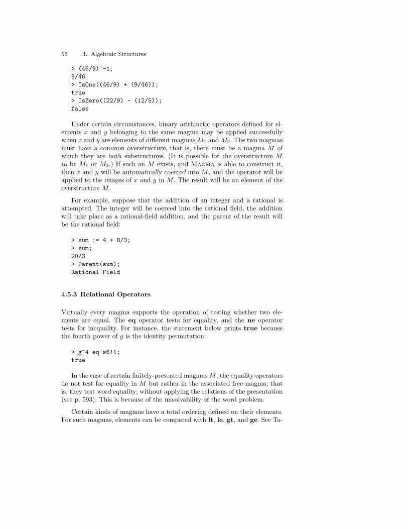
56 4. Algebraic Structures
> (46/9)^-1;9/46> IsOne((46/9) * (9/46));true> IsZero((22/9) - (12/5));false
Under certain circumstances, binary arithmetic operators defined for el-ements x and y belonging to the same magma may be applied successfullywhen x and y are elements of different magmas M1 and M2. The two magmasmust have a common overstructure, that is, there must be a magma M ofwhich they are both substructures. (It is possible for the overstructure Mto be M1 or M2.) If such an M exists, and Magma is able to construct it,then x and y will be automatically coerced into M , and the operator will beapplied to the images of x and y in M . The result will be an element of theoverstructure M .
For example, suppose that the addition of an integer and a rational isattempted. The integer will be coerced into the rational field, the additionwill take place as a rational-field addition, and the parent of the result willbe the rational field:
> sum := 4 + 8/3;> sum;20/3> Parent(sum);Rational Field
4.5.3 Relational Operators
Virtually every magma supports the operation of testing whether two ele-ments are equal. The eq operator tests for equality, and the ne operatortests for inequality. For instance, the statement below prints true becausethe fourth power of g is the identity permutation:
> g^4 eq s6!1;true
In the case of certain finitely-presented magmas M , the equality operatorsdo not test for equality in M but rather in the associated free magma; thatis, they test word equality, without applying the relations of the presentation(see p. 593). This is because of the unsolvability of the word problem.
Certain kinds of magmas have a total ordering defined on their elements.For such magmas, elements can be compared with lt, le, gt, and ge. See Ta-

4.5 Creating and Operating on Elements of a Magma 57
Table 4.4. Relational operators on elements of magmas
Magma Meaning
x eq y true if x = y
x ne y true if x 6= y
x lt y true if x < y (if defined)
x le y true if x ≤ y (if defined)
x gt y true if x > y (if defined)
x ge y true if x ≥ y (if defined)
IsZero(x) true if x is additive identity of M
IsId(x), IsIdentity(x) true if x is identity of group M
IsOne(x) true if x is multiplicative identity of ring M
ble 4.4. For instance, the following statement assigns false to bigger , because33100 is not greater than 1
3 :
> bigger := 33/100 gt 1/3;> bigger;false
The table also lists the functions IsZero(x), IsOne(x), IsIdentity(x)and IsId(x), which were included in the arithmetic tables too. These givethe same result as comparing x with the zero/one/identity element using eq,but may be more efficient.
If a relational operator is applied to elements x and y belonging to differentmagmas, the operation will only be legal if Magma can find a commonoverstructure for x and y, as explained on p. 56. In such a case, the operatorwill be applied to the images of x and y in the overstructure.
4.5.4 Canonical Forms of Elements
In the majority of categories in Magma, elements of a magma M are storedand returned in canonical form. That is, there is only one way in which agiven m ∈ M will be represented, and there is no concept of a ‘simplifiedform’ versus an ‘unsimplified form’ of m. For example:
> GF27<w> := GaloisField(27);> m1 := w^6 + w^3 + 1; m1;w^18> m2 := 2*w^5; m2;w^18> m1 eq m2;

58 4. Algebraic Structures
true
The exceptions to this rule are certain categories of finitely-presented(fp) magmas: fp semigroups, fp monoids, fp groups and fp algebras. In suchstructures, it is not always algorithmically possible to find canonical formsfor elements. (This restriction is known as the word problem.) Given a wordrepresenting an element, Magma only applies minimal simplifications (freereductions) to it before storing it. For example, in the finitely-presented groupbelow, the words assigned to w1 and w2 are not recognized by Magma asrepresenting the same element:
> bt<p, q> := Group< p, q | (p*q)^2 = p^3 = q^3 >;> w1 := p^7 * p^-2 * q^3; w1;p^5 * q^3> w2 := p^3 * q^5; w2;p^3 * q^5> w1 eq w2;false
4.5.5 Generators and Element Representation
With respect to the use of generators in the input representation and outputappearance of elements, it is convenient to recognize two distinct families ofmagma categories. The family to which a category belongs also influences themethods of creating elements of magmas in that category.
In the first family, the elements of magmas have a concrete output rep-resentation that does not explicitly display the generators. Categories suchas permutation groups, matrix rings, and vector spaces belong to this fam-ily. The output representation is usually an ordered collection of elementsfrom another magma (e.g., the coefficient ring), punctuated in a category-dependent way. The input representation for elements also tends not to re-quire explicit reference to the generators of the magma, although this ispermitted. For example:
> s5 := Sym(5);> s5elt := s5 ! (1, 5, 3)(2, 4);> s5elt2 := s5.2 * s5.1;> s5elt, s5elt2;(1, 5, 3)(2, 4)(1, 3, 4, 5)
> Z13 := ResidueClassRing(13);> Modu13 := RModule(Z13, 4);

4.5 Creating and Operating on Elements of a Magma 59
> Modu13elt := Modu13 ! [ 3, 9, 1, 7 ];> Modu13elt2 := 2*Modu13.3 - 5*Modu13.4;> Modu13elt, Modu13elt2;Modu13: (3 9 1 7)Modu13: (0 0 2 8)
Naming the generators using a generator assignment statement (p. 48) makesit easier for the user to form expressions in the generators, but does not affectthe appearance of output. Continuing the example:
> s5<a,b> := Sym(5);> s5elt2 := b * a; s5elt2;(1, 3, 4, 5)
> Modu13<p,q,r,s> := RModule(Z13, 4);> Modu13elt2 := 2*r - 5*s; Modu13elt2;Modu13: (0 0 2 8)
In the second family of categories, the magma M derives from an abstractfree structure, in which elements are represented in output as expressions inthe generators of M . This is the case particularly for finitely-presented mag-mas (including polynomial rings), which are quotients of free magmas, andwhose elements are exhibited as words (simple arithmetic expressions) in thegenerators of M . To create an element, the user must either express it explic-itly in terms of generators, or express it as a combination of previously-definedelements that were created directly or indirectly in terms of generators. As foroutput, the generators appear explicitly within each element that is printed;they are always identifiable, and so the appearance of generators in output isvery important in these categories. Magma’s default method of printing theith generator of a magma M is M .i (or $.i if it does not know the identifiername of M in that context). However, special generator names (identifiersand printnames) may be given by the user by means of the generator assign-ment statement, so as to make input easier and output more readable:
> gf25 := GF(25);> Generator(gf25);GF25.1> gf25.1 ^ 7;gf25.1^7
> Generator(GF(81));$.1> Random(GF(81));$.1^73

60 4. Algebraic Structures
> GF27<w> := GaloisField(27);> Generator(GF27);w> w ^ 7;w^7
4.6 Submagmas, Normal Closures and Ideals
Submagmas (subgroups, subrings etc.), normal closures and ideals of amagma M are created in very similar ways, so they are discussed together inthis section. In brief, a submagma, normal closure or ideal N may be built inMagma by means of a sub-constructor, ncl-constructor or ideal-constructorthat specifies M and a generating set S. The relationship between N and M isgiven by an inclusion monomorphism N → M , and this morphism is availableas the second return value of the constructor.
If the new magma N is a submagma or normal closure of M , its repre-sentation will be independent of M , but if N is an ideal of M it will retainsome connection to M . In any case, N will have its own generators, notatedeither by N .i or by the names chosen in a generator assignment statement.
For example, consider the K-matrix space m23 defined in the previoussection. Let N be the subspace of m23 generated by the matrices
A =
(5 2 643 8 9
)B =
(1 5 235 0 43
7
)
To create both N (naming the generators A and B) and the monomorphismi : N → m23 , the appropriate statement is:
> m23 := KMatrixSpace(RationalField(), 2, 3);> N<A,B>, i:=sub<m23 | [5,2,6,4/3,8,9], [1,5,23,5,0,43/7]>;> N;KMatrixSpace of 2 by 3 matrices and dimension 2over Rational Field> i;Mapping from: ModMatFld: N to ModMatFld: m23> A;[ 5 2 6][4/3 8 9]> B;[ 1 5 23][ 5 0 43/7]

4.6 Submagmas, Normal Closures and Ideals 61
> (N.1 eq A) and (N.2 eq B);true
These ideas will now be explained in more detail.
4.6.1 Creating Submagmas and Ideals
Let M be a magma. A submagma N of M is a magma in the same category asM such that there exists an inclusion monomorphism i : N → M . Informally,we can say that the elements of N are all elements of M , provided that weremember that the parent of these elements is N and not M . This is becauseeach magma exists in its own right (except for ideals), and the representationof the elements of N may be different from the representation of the elementsof M .
Given a subset S of M , there are several different substructures that arenaturally associated with M and S:
– The true submagma T of M generated by S, that is, the ‘smallest’ sub-magma of M containing S;
– The normal closure I generated by S, that is, the ‘smallest’ submagma ofM containing S that is normal in M . This structure is defined only if Mis a group.
– The ideal I generated by S, that is, the ‘smallest’ submagma of M con-taining S that is an ideal of M . This structure is defined only for certaincategories.
Magma offers a constructor for each of these substructures:
sub< M | specification of S >ncl< M | specification of S >ideal< M | specification of S >
If M has a non-commutative multiplication and is not a group, then idealdenotes the two-sided ideal, and the left ideal and right ideal constructorslideal and rideal are also available. For an example, see p. 531.
In these constructors, the magma M is given on the left of the | symbol.It is not necessary to create M first and then use an identifier; any expressionwhose value is M is suitable. On the right of the | symbol, the set S ofgenerators is specified, as a comma-separated list of expressions whose valuesare any of the following:
– An element of M ;

62 4. Algebraic Structures
– A sequence of primitive objects, as would be used for constructing a literalelement of M – interpreted as that element of M ;
– A set or sequence of elements of M ;
– A submagma or ideal of M – interpreted as the list of its generators, coercedinto M ;
– A set or sequence of submagmas and/or ideals of M .
Any normal syntax may be used in the list of expressions. When Magmaprocesses this list of generators, it removes repetitions of an element andoccurrences of the identity element. (If the list is empty or contains onlythe identity element, the trivial substructure will be returned.) Magma alsoplaces an ordering upon the generators, so that one can speak of the ith
generator.
For example, consider the matrix subring N described above, which wascreated as follows:
> N<A,B>, i:=sub<m23 | [5,2,6,4/3,8,9], [1,5,23,5,0,43/7]>;
The expressions on the right side of the | are sequences of primitive objects,as would be used for constructing literal elements of m23 . Another way tocreate N would be to assemble the generators in a set (or sequence) S first,and then to place S on the right side of the sub-constructor:
> S := m23 | [5,2,6,4/3,8,9], [1,5,23,5,0,43/7] ;> S;
[ 5 2 6][4/3 8 9],
[ 1 5 23][ 5 0 43/7]
> N<A,B>, i := sub< m23 | S >;
As another example, consider s6 , the symmetric group of degree 6, andthe element g = (2, 6, 4, 3) of s6 :
> s6 := Sym(6);> g := s6 ! (2,6,4,3);
The subgroup s6sub generated by g and (1, 5) can be built in Magma in thefollowing way:

4.6 Submagmas, Normal Closures and Ideals 63
> s6sub := sub< s6 | g, s6!(1, 5) >;> s6sub;Permutation group s6sub acting on a set of cardinality 6
(2, 6, 4, 3)(1, 5)
Here the expressions on the right side are elements of s6 . As it happens, itis possible to put (1, 5) instead of s6 !(1, 5) as one of these expressions, sinceit is a description of a literal element whose parent is clear from the context:
> s6sub := sub< s6 | g, (1, 5) >;
If the original magma M is not required in its own right, then there isno need to assign it to an identifier; any expression returning that magmamay be placed on the left side of the constructor. However, if it is necessaryto refer to M .i, the ith generator of M , on the right side of the constructor,then a where clause must be used to give M a temporary name:
> T := sub< V | [1,3,2,0,3,1], V.2 + V.4 >> where V is VectorSpace(GF(5), 6);
For an example of the difference between the sub-constructor and theideal-constructor, let R be the polynomial ring in x, y, z over Q, and let Tand I be the subring and ideal of R generated by the set S = x2− 2, x+ y:
> R<x,y,z> := PolynomialRing(RationalField(), 3);> T := sub< R | x^2 - 2, x + y >;> I := ideal< R | x^2 - 2, x + y >;> z*(x + y) in T;false> z*(x + y) in I;true
Note that some elements, such as z(x + y), are contained in I but not in T .
4.6.2 The Embedding in the Free Magma
Given a magma T , the function Generic(T ) returns its free or genericmagma, the magma in which T is naturally embedded. If T was created as asubstructure of M , Generic(T ) will only be M if M is free itself; otherwiseit will be the same as Generic(M).
For instance, suppose that s6subsub is constructed as the subgroup ofs6sub generated by g2. Magma considers s6subsub to be ultimately embeddedin the symmetric group of the same degree:

64 4. Algebraic Structures
> s6subsub := sub< s6sub | g^2 >;> s6subsub;Permutation group s6subsub acting on a set of cardinality 6
(2, 4)(3, 6)> s6 eq Generic(s6sub);true> s6 eq Generic(s6subsub);true
4.6.3 Inclusion Monomorphism and Principle of Locality
An important principle to keep in mind is that no matter how a magma iscreated (unless it is an ideal), its representation will be independent of anymagma from which it may have been created. This is the principle of locality.The principle of locality has the major advantage that if M is a submagmain the category C and T is a submagma of M , then T is a magma in thecategory C in its own right, and is not dependent on M ; thus any algorithmsapplying to magmas in C will apply to T .
For an example of the principle of locality, suppose M is a module ofdimension n over a field K. The standard representation for an n-dimensionalmodule over a field is in terms of the standard basis for K(n), so all theelements will be notated with n components:
> M := KModule(GF27, 5);> M;KModule M of dimension 5 over GF(3^3)> Random(M);M: ( w^7 w^25 w^11 w^8 2)
If T is created as an m-dimensional submodule of M , then T will be presentedrelative to the standard basis of K(m), rather than that of K(n). Thus all theelements of T will have m components:
> T := sub<M | [w^8, w^13, 2, 0, 1], [1, w, 0, w^19, w^2]>;> T;KModule T of dimension 2 over GF(3^3)> t := Random(T);> t;T: (w^18 w^14)
Now there is an obvious potential difficulty here. Since the elements ofT are represented independently of the elements of M , how is it possible to
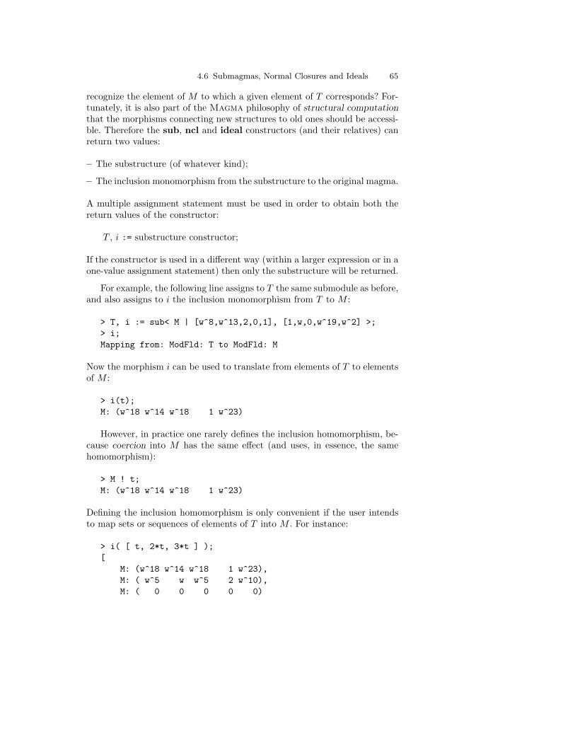
4.6 Submagmas, Normal Closures and Ideals 65
recognize the element of M to which a given element of T corresponds? For-tunately, it is also part of the Magma philosophy of structural computationthat the morphisms connecting new structures to old ones should be accessi-ble. Therefore the sub, ncl and ideal constructors (and their relatives) canreturn two values:
– The substructure (of whatever kind);
– The inclusion monomorphism from the substructure to the original magma.
A multiple assignment statement must be used in order to obtain both thereturn values of the constructor:
T , i := substructure constructor;
If the constructor is used in a different way (within a larger expression or in aone-value assignment statement) then only the substructure will be returned.
For example, the following line assigns to T the same submodule as before,and also assigns to i the inclusion monomorphism from T to M :
> T, i := sub< M | [w^8,w^13,2,0,1], [1,w,0,w^19,w^2] >;> i;Mapping from: ModFld: T to ModFld: M
Now the morphism i can be used to translate from elements of T to elementsof M :
> i(t);M: (w^18 w^14 w^18 1 w^23)
However, in practice one rarely defines the inclusion homomorphism, be-cause coercion into M has the same effect (and uses, in essence, the samehomomorphism):
> M ! t;M: (w^18 w^14 w^18 1 w^23)
Defining the inclusion homomorphism is only convenient if the user intendsto map sets or sequences of elements of T into M . For instance:
> i( [ t, 2*t, 3*t ] );[
M: (w^18 w^14 w^18 1 w^23),M: ( w^5 w w^5 2 w^10),M: ( 0 0 0 0 0)

66 4. Algebraic Structures
]
As another example, let G be the dihedral group of degree 16, repre-sented as a finitely-presented group with generators a and b, and let H bethe subgroup of G with generators c = a5b and d = ba−1:
> G<a,b> := DihedralGroup(GrpFP, 16);> G;Finitely presented group G on 2 generatorsRelations
a^16 = Id(G)b^2 = Id(G)(a * b)^2 = Id(G)
> H<c,d> := sub< G | a^5*b, b*a^-1 >;Finitely presented group H on 2 generatorsIndex in group G is 4 = 2^2Generators as words in group G
c = a^5 * bd = b * a^-1
Words of H are represented as products of the generators of H and theirinverses. For instance:
> h := c^3 * d^-2;> H eq Parent(h);true
To find the word of G corresponding to h, h must be coerced into G:
> G ! h;a^5 * b * a^5 * b * a^5 * b * a * b^-1 * a * b^-1
The result is a word of G. It can be seen to correspond to h because of theway that the generators c and d were defined.
4.7 Magma Generators
4.7.1 Generating Sets
In most algebraic categories, magmas are generally defined and represented interms of generating sets. If M is a magma, then the function returning the setof all generators of M is Generators(M), and NumberOfGenerators(M)

4.7 Magma Generators 67
or Ngens(M) returns how many of them there are. The elements of the setGenerators(M) are elements of M .
Although the generating set is a set rather than a sequence, its elementsmay be obtained in a fixed order for convenience in computation. The elementof M which is the ith generator of M is given by M .i, where i is a positiveinteger. This notation may always be used for input, and is sometimes used foroutput. (As demonstrated above, it is also possible to choose special namesfor generators.) Note that the order in which the set Generators(M) isprinted does not necessarily corresond to the M .i ordering. For instance:
> s5 := Sym(5);> Ngens(s5);2> Generators(s5);
(1, 2),(1, 2, 3, 4, 5)
> s5.1, s5.2;(1, 2, 3, 4, 5)(1, 2)
There are a few exceptions to these functions, however. Firstly, if the categoryof M indicates that M must have exactly one generator, these functionsare not used; instead, both Generator(M) and M .1 return the generator.Secondly, if the generators of M are not commonly thought of as generatorswithin this mathematical category, then some other function name is usedinstead, such as Rank(R) for the number of indeterminates of a polynomialring R:
> GF27<w> := GaloisField(27);> Generator(GF27);w
> R<x,y,z> := PolynomialRing(RationalField(), 3);> Rank(R);3
The generators available to the user in this way are not necessarily thoseused internally by Magma. In many categories, Magma distinguishes be-tween a foreground representation (used for input/output) and a backgroundrepresentation (used for computation), since algorithm designers have de-veloped special generating sets that are much more efficient than arbitrarygenerating sets for operations such as element membership tests. Examples

68 4. Algebraic Structures
are an echelonized basis for a vector space, and a base-and-strong-generating-set (BSGS) for a permutation group or finite matrix group. User access to theinternal representation depends on the category. However, the user’s chosenrepresentation is retained as far as possible for input and output.
4.7.2 Determination of the Generators
The way in which the generators of a magma M are determined and orderedby Magma depends on how M is constructed. There are several possibilities:
– M may be constructed as a free magma, in the strict sense of a magmawhose elements are represented as appropriate arithmetic combinations ofgiven generators;
– M may be returned by a call to a function that constructs certain standardexamples of magmas in a category (e.g., DihedralGroup);
– M may be built by means of a sub-constructor, ncl-constructor or ideal-constructor;
– M may arise from some other expression – no generalizations can be madeabout the generators of M in this situation.
In the first case, where M is a free magma, the number of generators isgiven by the context. For example:
> FG3 := FreeGroup(3);> FG3;Finitely presented group FG3 on 3 generators (free)> Generators(FG3); FG3.1, FG3.2, FG3.3
> R := PolynomialRing(RationalField(), 3);> R.1, R.2, R.3;$.1$.2$.3
> A4 := AbelianGroup([5,3,3,7]);> A4;Abelian Group isomorphic to Z/3 + Z/105Defined on 4 generatorsRelations:
5*A4.1 = 03*A4.2 = 0

4.7 Magma Generators 69
3*A4.3 = 07*A4.4 = 0
> Generators(A4);
A4.4,A4.2,A4.1,A4.3
From the abelian group example, note once again that the order in which thegenerating set is printed does not necessarily reflect the M .i ordering of thegenerators.
In the second case, where M is a standard magma, created by a functioninvocation, the generators are chosen by the algorithm designers. The usermust be familiar with the function in question in order to know the numberof generators and how they are chosen. For example:
> hamming := HammingCode(GF(2), 3);> Ngens(hamming);4> [ hamming.i : i in [1..4] ];[
(1 0 0 0 0 1 1),(0 1 0 0 1 0 1),(0 0 1 0 1 1 0),(0 0 0 1 1 1 1)
]
In the third case, where the magma M is built by means of one of thesubstructure constructors, the generating set bears some relation to the el-ements specified in the constructor. However, the elements described on theright side of the constructor belong to the original magma, whereas the setS′ given by Generators(M) is a set of elements of M . While S′ will bearsome relation to the constructor elements, it may not correspond precisely,for several reasons:
– identity elements will be removed (unless the identity is the only generator);
– repeated elements may be removed;
– other redundant elements (i.e., not independent of elements already listed)may also be removed, depending on the category;
– for ideals, extra generating elements may be required in addition to thosegiven in the constructor;

70 4. Algebraic Structures
– for polycyclic groups, if the elements given in the constructor are not ofthe correct form they will be replaced in S′ by pc-generators.
These phenomena are category-dependent, according to the appropriate algo-rithms for representing magmas in diffferent categories. The ordering of thesegenerators will be the same as the order in which the elements are listed onthe right side of the constructor, once the list has been modified accordingto the provisos above. (If an expression in this list is a set of elements thenthe generators will emerge in the standard iteration order for this set, andif an expression in the list is a magma then the generators will be orderedaccording to their generator-order for that magma.) In summary, then, ifthe elements described on the right side of the constructor are independent,non-trivial and in general suitably chosen, then the generators M .i will cor-respond to them, in the same order. Otherwise, the behaviour of Magma willdepend on the category.
For instance, in the example of the matrix space m23 and its subspace N ,if the generators listed for the construction of N are ‘sensible’ then they willbe taken as the generators of N (but as elements of N , rather than elementsof m23 ):
> m23 := KMatrixSpace(RationalField(), 2, 3);> N := sub<m23 | [5,2,6,4/3,8,9], [1,5,23,5,0,43/7]>;> N.1, N.2;[ 5 2 6][4/3 8 9]
[ 1 5 23][ 5 0 43/7]
However, if there are unnecessary elements listed in the constructor thenthe correspondence may be less direct. The following pair of examples illus-trates how the correspondence breaks down if the list specifying the genera-tors includes repeated elements, non-independent elements and the identity:
> GF27<w> := GaloisField(27);> VS4 := VectorSpace(GF27, 4);> v := VS4 ! [w^14, 2, w^3, 1];> VS4s := sub< VS4 | v, 0, 2*v, v >;> Ngens(VS4s);3> VS4s.1, VS4s.2, VS4s.3;(w^14 2 w^3 1)( w 1 w^16 2)(w^14 2 w^3 1)

4.7 Magma Generators 71
> Generators(VS4s);
( w 1 w^16 2),(w^14 2 w^3 1)
> Basis(VS4s);[
( 1 w^25 w^15 w^12)]
> s5 := Sym(5);> s5s := sub< s5 | (1,2,3), 1, (1,2,3)^2, (1,2,3) >;> Ngens(s5s);2> s5s.1, s5s.2;(1, 2, 3)(1, 3, 2)> Generators(s5s);
(1, 2, 3),(1, 3, 2)
In both examples, the numbering of the generators does not correspond towhat might immediately be expected, nor is it the same in these two cat-egories: the fourth generator becomes the third generator in the first caseand the second generator in the second case. In the vector space case, thezero is removed, and then the numbering of the generators corresponds to allthe remaining generators (including the repeated generator). However, theGenerators function returns a two-element set, since there are only two dis-tinct generators. Note also that the basis, which is the internal representationof the generators, contains only one element. On the other hand, in the per-mutation group case both the identity and the repeated element are removed,whereas in the vector space example the repeated element was retained. Thegenerator set still contains a redundancy, but after the initial construction ofthe group and its BSGS the efficiency of Magma’s computations would notbe impaired by this.
When constructing normal closures and ideals, Magma often needs toadd extra elements to the given generating set. For example, consider thenormal closure of the submagma of s5 generated by (1, 2, 3) and (1, 3)(2, 4):
> s5n := ncl< s5 | (1,2,3), (1,3)(2,4) >;> Ngens(s5n);3

72 4. Algebraic Structures
> s5n.1, s5n.2, s5n.3;(1, 2, 3)(1, 3)(2, 4)(3, 5, 4)> Generators(s5n);
(1, 2, 3),(3, 5, 4),(1, 3)(2, 4)
The submagma generated by (1, 2, 3) and (1, 3)(2, 4) alone is not normal in s5 ,so Magma must enlarge that submagma with extra generators. It providesthe generator (3, 5, 4), and places it on the end of the generator list, so thatthe two generators given by the user are numbered first and second.
4.7.3 Remarks on Generator Names
Recall from p. 58 that there are two families of magma categories with respectto the input and output representation of their elements. When a magma Mis assigned using a generator assignment statement, the behaviour of thisstatement depends on the family to which the category of M belongs.
In the first family of categories, the magma elements have a concreterepresentation that does not explicitly display the generators. If the categoryof M is in this family, a generator assignment statement will assign M itself,and assign its generators to identifiers with the given names. For example,consider the ring of complex numbers with integral coefficients. It may berepresented as the subring of the 2 × 2 matrices in which A + BI maps to(
A B
−B A
)and, in particular, I maps to the generator
(0 1
−1 0
). Thus
it is logical to name the generator with the identifier I:
> gaussians<I> :=> sub< MatrixRing(IntegerRing(), 2) | [0, 1, -1, 0] >;> gaussians;Matrix Algebra of degree 2 with 1 generatorover Integer Ring> Generators(gaussians);
[ 0 1][-1 0]
> I^2;

4.7 Magma Generators 73
[-1 0][ 0 -1]> gaussians ! (-1);[-1 0][ 0 -1]
In the second family of categories, the output representation of magmaelements is always explicitly in terms of generators, and the input represen-tation is directly or indirectly in terms of generators. If the category of M isin this family, a generator assignment statement will assign M itself, assignits generators to identifiers with the given names, and cause the generatorsto be printed with the given names. For example:
> Q := RationalField();> R := PolynomialRing(Q, 3);> f := R.1*R.2 + R.2*R.3 + R.1*R.3;> f;$.1*$.2 + $.1*$.3 + $.2*$.3
> R<x,y,z> := PolynomialRing(Q, 3);> f := x*y + y*z + x*z;> f;x*y + x*z + y*z
If a magma M in the second family is created without naming its gener-ators, and the user then realizes that the generators need printnames, it ispossible to provide them using the procedure AssignNames(˜M,Q), whereQ is a sequence of the generator names given as strings. This does not createidentifiers with these names; it only changes the printnames. For example:
> A := AbelianGroup([4,7,8]);> A;Abelian Group isomorphic to Z/4 + Z/56Defined on 3 generatorsRelations:
4*A.1 = 07*A.2 = 08*A.3 = 0
> A.1 + 2*A.3;A.1 + 2*A.3> AssignNames(~A, ["k", "l", "m"]);> A;Abelian Group isomorphic to Z/4 + Z/56Defined on 3 generatorsRelations:

74 4. Algebraic Structures
4*k = 07*l = 08*m = 0
> A.1 + 2*A.3;k + 2*m
Note that the generators must still be described in input using the A.i syntax,since AssignNames does not create identifiers called k, l,m. However, theuser could manually assign the generators to identifiers:
> k := A.1; l := A.2; m := A.3;
The user should take care not to reassign a generator name. AlthoughMagma will permit this, and the generator will still be accessible via theM .i syntax, the subsequent output may be confusing. For the second familyof categories, the printname will remain the same even though the identifierno longer has its former value. For example:
> R<x,y,z> := PolynomialRing(Q, 3);> 3*x*y^2 + z^3;3*x*y^2 + z^3> x := 17;> x;17> R.1;x> 3*x*y^2 + z^3;51*y^2 + z^3> 3*R.1*y^2 + z^3;3*x*y^2 + z^3
4.7.4 The Pseudo-Identifier $
Magma output sometimes contains the character $, to indicate a namelessmagma. It does this when the magma has not been assigned to an identifier,or when it cannot locate the identifier to which it was assigned. For instance:
> Generators(FreeMonoid(6)); $.1, $.2, $.3, $.4, $.5, $.6
> FM6 := FreeMonoid(6);> Generators(FM6); FM6.1, FM6.2, FM6.3, FM6.4, FM6.5, FM6.6

4.8 Quotient Magmas 75
4.8 Quotient Magmas
Let M be a magma, and let I be the normal subgroup or ideal of M generatedby the set S of elements of M . The quotient magma Q = M/I may be createdwith the quo-constructor:
quo< M | specification of S >
The rules for the specification of S are exactly the same as they are forthe sub, ncl and ideal constructors. Magma uses these elements of M togenerate I, expanding the generating set if necessary to obtain a substructurethat is normal/ideal in M . Then Magma uses M and I to create the quotientmagma Q.
For example, let cube be the group of symmetries of the cube, representedas a permutation group on the 8 vertices, with generators a, b, c:
> cube<a, b, c> := sub< Sym(8) | (1, 2, 3, 4)(5, 6, 7, 8),> (2, 4, 5)(3, 8, 6), (1, 5)(2, 6)(3, 7)(4, 8) >;> cube;Permutation group cube acting on a set of cardinality 8
(1, 2, 3, 4)(5, 6, 7, 8)(2, 4, 5)(3, 8, 6)(1, 5)(2, 6)(3, 7)(4, 8)
The following statement constructs quotgp as the quotient of cube by thenormal closure generated by a2, c, cb:
> quotgp := quo< cube | a^2, c, c^b >;> quotgp;Permutation group quotgp acting on a set of cardinality 6Order = 6 = 2 * 3
(1, 2)(3, 5)(4, 6)(1, 3, 6)(2, 4, 5)
Like sub, ncl and ideal, the quo-constructor returns a homomorphismas its second return value. This homomorphism is the natural homomorphismφ : M → Q. It is obtained by means of a multiple assignment statement:
Q, n := quo< magma | specification of S >;
Continuing the example:
> quotgp, natl := quo< cube | a^2, c, c^b >;> natl;

76 4. Algebraic Structures
Mapping from: GrpPerm: cube to GrpPerm: quotgp> natl(a * b);(1, 4)(2, 3)(5, 6)
The natural homomorphism may also be used to map sets or sequences ofelements of M , or submagmas of M , to sets or sequences of Q, or submagmasof Q. For instance:
> sq := [ cube | (1,6)(4,7), (1,6,8)(2,7,4), (1,8)(2,7) ];> natl(sq);[
(1, 4)(2, 3)(5, 6),(1, 3, 6)(2, 4, 5),(1, 5)(2, 6)(3, 4)
]> natl(sub< cube | a * c >);Permutation group acting on a set of cardinality 6
(1, 2)(3, 5)(4, 6)
Furthermore, it is possible to calculate preimages of these with the @@ oper-ator:
> ncl< quotgp | (1, 3, 6)(2, 4, 5) > @@ natl;Permutation group acting on a set of cardinality 8
(1, 3)(2, 4)(5, 7)(6, 8)(1, 5)(2, 6)(3, 7)(4, 8)(2, 4, 5)(3, 8, 6)(1, 2)(3, 4)(5, 6)(7, 8)
These mapping operations are explained in more detail in Chapter 7.
If the user is constructing a quotient by an ideal or normal closure Ibut wishes I to be assigned to an identifier, the best way to use the quo-constructor is to create I first, via ideal or ncl, and then to put I as thespecification of S in the quo-constructor. The quo-constructor will extractthe generators of I in order to construct the quotient. For example:
> I := ncl< cube | a^2, c, c^b >;> quotgp eq quo< cube | I >;true
As another example, consider the problem of constructing the quotient ofa vector space. After the following initial assignments:
> V5 := VectorSpace(RationalField(), 5);

4.8 Quotient Magmas 77
> V5;Full Vector space of degree 5 over Rational Field> u1 := V5 ! [23/5, -2, 8, 0, 0];> u2 := V5 ! [-2/5, 0, 1, -4, 0];
these two collections of statements produce the same quotient space Q5 andnatural homomorphism n:
> Q5, n := quo< V5 | u1, u2 >;> Q5;Full Vector space of degree 3 over Rational Field
> W5 := sub< V5 | u1, u2 >;> Q5, n := quo< V5 | W5 >;> Q5;Full Vector space of degree 3 over Rational Field
Note that since every subspace of a vector space is normal, a sub-constructoris used for W5 rather than an ideal-constructor. The natural homomorphismn may be used to map between parts of the structures. Observe that itskernel, returned by the function Kernel(n), is the ideal from which Magmaconstructed the quotient:
> Kernel(n) eq W5;true
It is important to realize that the quotient magma is not a substructureof the original M , unlike a magma returned by sub, ncl or ideal. In the firstexample above, cube and quotgp are both represented as permutation groups,but cube is acting on a set of cardinality 8 whereas quotgp is acting on a setof cardinality 6. In the second example, V5 and Q5 are both vector spaces,but the number of components in the vectors is different.
Moreover, for many categories of magma, the Magma representation ofa quotient of M may not lie in the same category as M does. This occursbecause the representation and/or operations on elements of the quotientmagma are different. Consider, for example, the polynomial ring P = Q[x],and an element f of P . Elements of a quotient Pq relative to the ideal Igenerated by f are standard representatives of the cosets of I. Thus Pq isin a different category, the category RngUPolRes of residue classes of aunivariate polynomial ring. The multiplication of elements in Pq is achievedby multiplying the polynomial-representatives and then taking the remainderupon division by f . For instance:
> P<x> := PolynomialRing(RationalField());

78 4. Algebraic Structures
> f := x^3 + 5;> Pq<y> := quo< P | f >;> Pq;Univariate Quotient Polynomial Algebra in yover Rational Fieldwith modulus y^3 + 5> Category(P), Category(Pq);RngUPol RngUPolRes
> p1 := 5*x^9 - 6*x^5 + 2*x^3 + x^2 - 7;> p2 := 5*x^2 + x - 1;> q1 := Pq ! p1; q1;31*y^2 - 642> q2 := Pq ! p2; q2;5*y^2 + y - 1> (p1 * p2) mod f;-3241*x^2 - 1417*x + 487> q1 * q2;-3241*y^2 - 1417*y + 487
4.9 Shorthand Constructors
For many categories, shorthand constructors are provided that allow anymagma to be constructed in a single step. Implicitly, the construction iseither as a finitely-presented magma (i.e., a quotient of a free magma), oras a submagma of a generic magma. However, the user does not have toconstruct the free or generic magma explicitly.
4.9.1 Finitely-Presented Magmas
Let M be a magma belonging to an algebraic variety V . A well-known the-orem states that V contains free algebras and that M is isomorphic to aquotient of some free algebra F . A description of M as a quotient of a freealgebra will be called a presentation. Informally, a presentation consists ofthe free algebra F and a set S of elements of F whose ideal closure I has theproperty that M ∼= F/I. If S is finite, then M is said to be finitely-presented.
The construction of a finitely-presented magma from first principlesinvolves constructing the corresponding free magma and then taking asuitable quotient. For instance, the group G given by the presentation〈c, d | c2, d3, (cd)4〉 can be created as a quotient of the free group F on twogenerators:

4.9 Shorthand Constructors 79
> F<a,b> := FreeGroup(2);> G<c,d> := quo< F | a^2, b^3, (a*b)^4 >;> G;Finitely presented group G on 2 generatorsRelations
c^2 = Id(G)d^3 = Id(G)(c * d)^4 = Id(G)
However, since the construction of finitely-presented magmas is so fre-quently performed, there are shorthand constructors provided, allowing thedirect construction of the finitely-presented magma from its presentationwithout explicitly building the free magma first. The categories having theshorthand form are GrpFP, SgpFP, MonFP, GrpPC, and GrpAb (i.e.,finitely-presented groups, semigroups, monoids, polycyclic groups and abeliangroups). The syntax is:
constructor-word< generators | relations >
where the word on the left of the constructor may be any one of Group,Semigroup, Monoid, PolycyclicGroup or AbelianGroup. The genera-tors are a comma-separated list of identifiers, which are used as the generatornames in the relations appearing on the right side of the constructor; thenumber of generators indicates the rank of the corresponding free magma.The relations, whose syntax depends on the category, are given in a comma-separated list on the right of the constructor. A relation may be of the formwL=wR, where wL and wR are words in the generators; if the free magma hasan identity, then the word w by itself is understood to mean that w equalsthe identity; relation lists w1=w2= · · · =wk may also be permitted.
Generator assignment is still necessary if the generators are to have specialnames; the scope of the generator names used in the constructor is restrictedto the constructor. It does not matter whether or not the same generatornames are used inside and outside the constructor.
Examples are given for each of the possible categories:
> G<c,d> := Group< a, b | a^2, b^3, (a*b)^4 >;> G;Finitely presented group G on 2 generatorsRelations
c^2 = Id(G)d^3 = Id(G)(c * d)^4 = Id(G)
> SG<s,t> := Semigroup< s, t | s^7 = t^4, s*t = t*s^2 >;

80 4. Algebraic Structures
> SG;Finitely presented semigroupRelations
s^7 = t^4s * t = t * s^2
> M<A,B,C> :=> Monoid< a, b, c | a^5, b^2*c = a^3*c*b = b*a*b*c >;> M;Finitely presented monoidRelations
A^5 = Id(M)B^2 * C = B * A * B * CA^3 * C * B = B * A * B * C
> PG<e,f> := PolycyclicGroup< e, f | e^2, f^3, f^e=f^2 >;> PG;GrpPC : PG of order 6 = 2 * 3PC-Relations:
e^2 = Id(PG),f^3 = Id(PG),f^e = f^2
> A<x,y,z> := AbelianGroup< x, y, z | 2*y=4*x, x+10*y >;> A;Abelian Group isomorphic to Z/42 + ZDefined on 3 generatorsRelations:
x + 10*y = 042*y = 0
Like the quo-constructor, these shorthand constructors return the naturalhomomorphism as their second return value. The domain of the homomor-phism is always the corresponding free magma:
> A<x,y,z>, n := AbelianGroup< x, y, z | 2*y=4*x, x+10*y >;> n;Mapping from: Abelian Group isomorphic to Z + Z + ZDefined on 3 generators (free)toAbelian Group isomorphic to Z/42 + ZDefined on 3 generatorsRelations:
$.1 + 12*$.2 = 042*$.2 = 0

4.9 Shorthand Constructors 81
4.9.2 Submagmas of Generic Magmas
A similar shorthand device applies for some categories that have genericmagmas: matrix groups, matrix algebras (matrix rings), permutation groups,and linear codes. However, the magma constructed is a submagma of thegeneric magma, not a quotient. The syntax for these shorthand constructorsis:
constructor-word< generic magma specification | generators >
The submagma generators on the right of the constructor may be ex-pressed in the same way as for a sub-constructor. The generic magmaspecification on the left of the constructor is category-dependent, but itrelates to the arguments given to the function that constructs the genericmagma. If the constructor-word is MatrixGroup, the information requiredis the degree followed by the coefficient ring, as for GL(n,R); if it isMatrixAlgebra (or equivalently MatrixRing), the information requiredis the coefficient ring followed by the degree, as for MatrixAlgebra(R, d);if it is PermutationGroup, the degree is required, as for Sym(n); if it isLinearCode, the finite field and length are required, as for the functionVectorSpace(K, n).
In most of these categories, the shorthand constructor returns the inclu-sion monomorphism from the new magma to the generic magma as its secondreturn value, just as if the sub-constructor had been applied.
Examples are:
> K<w> := FiniteField(9);> H, i := MatrixGroup< 3, K |> [1,w,0, 0,1,0, 1,w^2,1], [w,0,0, 0,1,0, 0,0,w] >;> H;MatrixGroup(3, GF(3^2))Generators:
[ 1 w 0][ 0 1 0][ 1 w^2 1]
[ w 0 0][ 0 1 0][ 0 0 w]
> i;Mapping from: GrpMat: H to GL(3, GF(3, 2))
> A, i := MatrixAlgebra< RationalField(), 3 |

82 4. Algebraic Structures
> [ 1/3,0,0, 3/2,3,0, -1/2,4,3 ],> [ 3,0,0, 1/2,-5,0, 8,-1/2,4 ] >;> A : Maximal;Matrix Algebra of degree 3 with 2 generatorsover Rational FieldGenerators:[ 1/3 0 0][ 3/2 3 0][-1/2 4 3]
[ 3 0 0][ 1/2 -5 0][ 8 -1/2 4]> i;Mapping from: AlgMat: A toFull Matrix Algebra of degree 3 over Rational Field
> G, i := PermutationGroup< 9 | (2,4)(6,8), (1,3,5,7,9) >;> G;Permutation group acting on a set of cardinality 9
(2, 4)(6, 8)(1, 3, 5, 7, 9)
> Domain(i), Codomain(i);Permutation group G acting on a set of cardinality 9
(2, 4)(6, 8)(1, 3, 5, 7, 9)
Symmetric group acting on a set of cardinality 9Order = 362880 = 2^7 * 3^4 * 5 * 7
> Q := [ [1,0,0,0,0,1,1], [0,1,0,0,1,0,1],> [0,0,1,0,1,1,0], [0,0,0,1,1,1,1] ];> LinearCode< GF(2), 7 | Q >;[7, 4, 3] Hamming code (r = 3) over GF(2)Generator matrix:[1 0 0 0 0 1 1][0 1 0 0 1 0 1][0 0 1 0 1 1 0][0 0 0 1 1 1 1]
4.10 Some Other Operations on Magmas
Table 4.5 summarizes the principal operators and functions that apply to(nearly) all magmas. They are illustrated below.

4.10 Some Other Operations on Magmas 83
Table 4.5. Operations on magmas
Magma Meaning
#M Number of elements of finite magma M
L eq M true if magmas L and M are equal
L ne M true if L and M are not equal
L cmpeq M true if L eq M is true; else false
x in M true if x is an element of M
x notin M true if x is not an element of M
L subset M true if elements of L are all in M
L notsubset M true if elements of L are not all in M
L meet M Intersection of L and M
Rep(M) An arbitrary element of M (the same each time)
Random(M) A random element of finite magma M
Set(M) Set of elements of finite magma M
FormalSet(M) Formal set of elements of magma M
If an expression returning a finite magma is preceded by the operator#, Magma will return the cardinality of the magma, that is, the numberof elements it has. (If M is a group, Order(M) is a synonym for #M .)For instance, the following output verifies that the finite field of size 24 doesindeed have 16 elements:
> #GF(2, 4);16
Given two comparable magmas L and M , the expression L meet Mreturns their intersection, that is, the magma whose elements are the elementscommon to L and M . Normally, the intersection will satisfy the same axiomsas the magmas from which it was built. For instance, when two subspacesof the vector space V5 created above are intersected, the result is also asubspace of V5 :
> V5 := VectorSpace(RationalField(), 5);> u1 := V5 ! [23/5, -2, 8, 0, 0];> u2 := V5 ! [-2/5, 0, 1, -4, 0];> W5 := sub< V5 | u1, u2 >;> X5 := sub< V5 | u1+u2, V5![6, -2, -1/5, 0, 3] >;> W5 meet X5;Vector space of degree 5, dimension 1 over Rational FieldEchelonized basis:( 1 -10/21 15/7 -20/21 0)
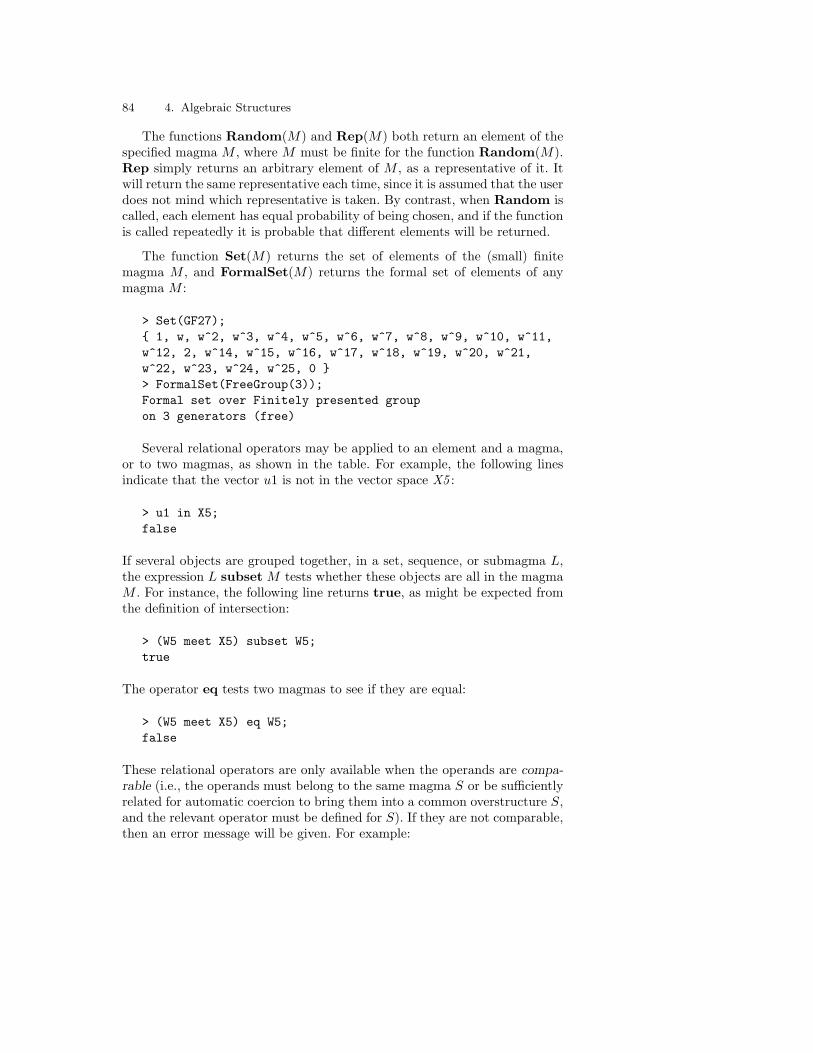
84 4. Algebraic Structures
The functions Random(M) and Rep(M) both return an element of thespecified magma M , where M must be finite for the function Random(M).Rep simply returns an arbitrary element of M , as a representative of it. Itwill return the same representative each time, since it is assumed that the userdoes not mind which representative is taken. By contrast, when Random iscalled, each element has equal probability of being chosen, and if the functionis called repeatedly it is probable that different elements will be returned.
The function Set(M) returns the set of elements of the (small) finitemagma M , and FormalSet(M) returns the formal set of elements of anymagma M :
> Set(GF27); 1, w, w^2, w^3, w^4, w^5, w^6, w^7, w^8, w^9, w^10, w^11,w^12, 2, w^14, w^15, w^16, w^17, w^18, w^19, w^20, w^21,w^22, w^23, w^24, w^25, 0 > FormalSet(FreeGroup(3));Formal set over Finitely presented groupon 3 generators (free)
Several relational operators may be applied to an element and a magma,or to two magmas, as shown in the table. For example, the following linesindicate that the vector u1 is not in the vector space X5 :
> u1 in X5;false
If several objects are grouped together, in a set, sequence, or submagma L,the expression L subset M tests whether these objects are all in the magmaM . For instance, the following line returns true, as might be expected fromthe definition of intersection:
> (W5 meet X5) subset W5;true
The operator eq tests two magmas to see if they are equal:
> (W5 meet X5) eq W5;false
These relational operators are only available when the operands are compa-rable (i.e., the operands must belong to the same magma S or be sufficientlyrelated for automatic coercion to bring them into a common overstructure S,and the relevant operator must be defined for S). If they are not comparable,then an error message will be given. For example:

4.11 Warning About Large Magmas 85
> "w" in WittDesign(12);
>> "w" in WittDesign(12);^
Runtime error in ’in’: Bad argument types> MatrixRing(GF(2), 3) eq Sym(6);
>> MatrixRing(GF(2), 3) eq Sym(6);^
Runtime error in ’eq’: Bad argument types
There is an additional relational operator, cmpeq, which is designed forsuch purposes as testing the suitability of arguments in function/procedureinvocations. It is similar to eq, but never gives an error message if the ar-guments are incomparable. The value of L cmpeq M is true whenever thevalue of L eq M is true; otherwise, its value is false, no matter whether L eqM would return false or give an error message. Another way to view this op-erator is that it returns true only if L and M have a common overstructureS, eq is defined for the category of S, and L eq M is true; it returns falseotherwise. For example:
> W5 cmpeq W5;true> MatrixRing(GF(2), 3) cmpeq Sym(6);false
Further operations on magmas are explained in later chapters of thisbook, since they are more dependent on the category or variety. However,this book cannot explain every feature; see the Handbook or the online helpfor a complete account of the system.
4.11 Warning About Large Magmas
Magma has been designed to perform efficient computations, even on mag-mas which are very large. For instance, given a permutation group, it con-structs a concise representation rather than a physical list of its elements,to save speed and time. Moreover, once a piece of information has been con-structed for some magma, it is usually cached automatically, for subsequentreference. Nonetheless, calculations on large magmas can often consume sig-nificant amounts of computer time and/or storage space.
When working with small magmas in Magma, it does not matter if unnec-essary or inefficient calculations are performed, because the execution time

86 4. Algebraic Structures
and storage space used will be insignificant. It is with very large magmas thatcare is required. Before writing a program to build a standard mathematicalobject, the user should check whether Magma already provides a function oroperator that performs the desired task. The Magma version will probablybe faster than the user’s own version, since the algorithm is likely to be theproduct of extensive research, and since Magma can make the most of itsinformation storage techniques.

5. Conditional Statements and Expressions
One of the major purposes of Boolean values is to manage the flow of con-trol in a program. Conditional statements and expressions use the results ofBoolean tests in order to decide which statement to perform next, or whichexpression to evaluate. The main conditional statement in Magma is theif-statement, and the main conditional expression is the select-expression.Also provided are a case-statement and a case-expression, which are usedwhen there are several possible courses of action, depending on the value ofsome expression.
The examples given in this chapter of conditionals are rather artificial.The utility of these constructions will be seen once user-defined functionsand procedures are introduced in Chapter 8.
5.1 The if-statement
5.1.1 Basic Form of the if-statement
Magma’s if-statement causes Magma to perform different actions dependingon whether a certain condition is true or false. The if-statement has severalsyntactic forms, the most basic of them being:
if condition thenstatements
elsestatements
end if;
The statements between then and else are executed if the condition is true,and the statements between else and end if are executed if the conditionis false. Note that, like all other statements, the if-statement ends with asemicolon. The newlines and indentation are optional, and are ignored byMagma, but they tend to make the code easier to read.
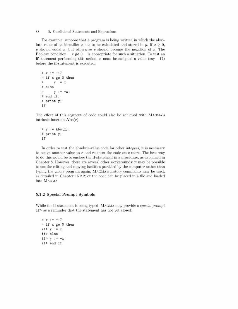
88 5. Conditional Statements and Expressions
For example, suppose that a program is being written in which the abso-lute value of an identifier x has to be calculated and stored in y. If x ≥ 0,y should equal x, but otherwise y should become the negation of x. TheBoolean condition x ge 0 is appropriate for such a situation. To test anif-statement performing this action, x must be assigned a value (say −17)before the if-statement is executed:
> x := -17;> if x ge 0 then> y := x;> else> y := -x;> end if;> print y;17
The effect of this segment of code could also be achieved with Magma’sintrinsic function Abs(r):
> y := Abs(x);> print y;17
In order to test the absolute-value code for other integers, it is necessaryto assign another value to x and re-enter the code once more. The best wayto do this would be to enclose the if-statement in a procedure, as explained inChapter 8. However, there are several other workarounds: it may be possibleto use the editing and copying facilities provided by the computer rather thantyping the whole program again; Magma’s history commands may be used,as detailed in Chapter 15.2.2; or the code can be placed in a file and loadedinto Magma.
5.1.2 Special Prompt Symbols
While the if-statement is being typed, Magma may provide a special promptif> as a reminder that the statement has not yet closed:
> x := -17;> if x ge 0 thenif> y := x;if> elseif> y := -x;if> end if;

5.1 The if-statement 89
> print y;17
(Magma behaves in a similar way for other incomplete statements, such asthe while and for statements explained in Chapter 9.) This prompt wasturned off in the program listing above, so that the program would be easierto read; this convention will be followed throughout this book. The procedureSetPrompt(P ), where P is a string, may be used to control the style ofprompt. To request the simple prompt, the user should type
> SetPrompt("> ");
and to request the prompt which gives a reminder about which statementshave not yet closed, the user should type
> SetPrompt("%S> ");
5.1.3 Short Form of the if-statement
If a program requires an if-statement for which there is no action to be takenif the condition is false, a shorter form of the if-statement should be used.This shorter form simply omits the else clause:
if condition thenstatements
end if;
For example, the absolute value code above could be rewritten as follows:
> x := -54;
> y := x;> if x lt 0 then> y := -y;> end if;> print y;54
5.1.4 Avoiding Nested if-statements
Sometimes the else clause of an if-statement will itself be an if-statement.At the end of such an if-statement there would be matching end if; closures.

90 5. Conditional Statements and Expressions
This type of nested if-statement may be avoided by making use of elif, whichis a shorter form of else if that also removes the need for an end if to closeoff the inner if-statement:
if condition thenstatements
elif condition thenstatements
elif condition thenstatements...
elsestatements
end if;
For example, an if-statement with elif clauses may be used to convertfrom a percentage mark into a grade. The program assumes that mark hasbeen assigned an integer in the range 0, . . . , 100:
To perform this example online, type load "I96c5e1";
> if mark ge 85 then> print "High Distinction";> elif mark ge 75 then> print "Distinction";> elif mark ge 65 then> print "Credit";> elif mark ge 50 then> print "Pass";> else> print "Fail";> end if;
5.1.5 Longer Example: Area of a Triangle
The next example of the if-statement is a procedure TriangleArea(a, b, c)that, given the side-lengths a, b, c of a triangle, calculates and prints the areaof the triangle. It uses the formula Area =
√s(s− a)(s− b)(s− c), where s
equals (a + b + c)/2. To check that the triangle exists, it checks that the sumof the two smaller sides is greater than or equal to the third side. (If they areequal, the triangle is degenerate.)

5.1 The if-statement 91
The code has been written as a procedure so that it can be tested easily forseveral choices of side-lengths. The first and last lines handle the procedure-aspect of the code, and should not cause confusion.
The first two lines of the procedure body (i.e., the second and third linesof the program) are sequence manipulations (see Chapter 6) whose purpose isto assign A,B, C the same values as a, b, c, but sorted from lowest to highest.Explode(Q) is a multiple return value function that returns the first term,the second term, the third term, and so on, of a given sequence Q.
To perform this example online, type load "I96c5e2";
> TriangleArea := procedure(a, b, c)> Q := Sort([a, b, c]);> A, B, C := Explode(Q);> sumAB := A + B;> if sumAB lt C then> print "No triangle has these side-lengths.";> elif sumAB eq C then> print "Triangle is degenerate (straight line).";> print "Area is 0 square units.";> else> s := (A+B+C)/2;> print "Area is", Sqrt(s*(s-A)*(s-B)*(s-C)),> "square units.";> end if;> end procedure;
The procedure TriangleArea(a, b, c) may be called by supplying suitableexpressions for a, b and c. For example:
> TriangleArea(6, 8, 10);Area is 24.00000000000000000000000000 square units.> TriangleArea(10.2, 12, 14.5);Area is 60.466393507054809296259993289470 square units.> TriangleArea(6, 20, 3);No triangle has these side-lengths.> TriangleArea(13, 9, 4);Triangle is degenerate (straight line).Area is 0 square units.
The figures in the output have a rather large number of digits because thearguments are elements of the real field (or coerced into it for the squareroot computation), which has default precision 28. This precision could beadjusted if required.

92 5. Conditional Statements and Expressions
5.2 The select-expression
The if-statement is a very flexible statement. It can be used whenever theaction to be performed depends on the truth of some expression. However,if the only action of the if-statement is to assign or print the value of anexpression, it is sufficient to use a conditional expression instead. The mostcommon form of conditional expression in Magma is the select-expression:
condition select expression else expression
and it has the value calculated from the first expression if the condition istrue, and the value from the second expression if the condition is false. Sincea select-expression can be used as part of a longer expression, it can be veryconvenient for such tasks as constructing sets and sequences.
For instance, the first example in this section could also be programmedas follows:
> y := x ge 0 select x else -x;
To evaluate this statement, Magma first tests the x ge 0 condition. If it istrue, then y is assigned the first value, x, and otherwise y is assigned thesecond value, −x. For instance:
> x := 42;> y := x ge 0 select x else -x;> print y;42> x := -9;> y := x ge 0 select x else -x;> print y;9
Like the operators and and or, the select-expression uses call-by-nameevaluation. That is, it does not evaluate both the expressions following select,only the one specified by the truth or falsity of the initial condition.
5.3 The case-statement
The case-statement is rather like the elif variety of the if-statement, but itis used when the action depends on which of several values is equal to a givenvalue. The syntax of the case-statement is:

5.3 The case-statement 93
case expression:when expression, . . . , expression:
statementswhen expression, . . . , expression:
statements...else
statementsend case;
The else clause is optional.
To execute this statement, Magma evaluates the expression given aftercase. It successively compares the value of this expression with the valuesof the expressions given after each when. If it finds a match, Magma exe-cutes the statements following the corresponding when. If none of the valuesmatch, Magma executes the statements after else, or does nothing if theelse clause is absent.
Magma executes at most one of the blocks of statements in a case-statement. If more than one of the when options contains an expressionwhose value equals the value of the case expression, Magma will only executethe statements corresponding to the first of these when options, starting fromthe top.
For example, the TriangleArea(a, b, c) procedure constructed above maybe modified to use a case-statement. The expression given after case isSign(A + B − C), since it is the sign of A + B − C that governs whichstatements should be executed. The intrinsic function Sign(x) returns 1, 0or −1 according to whether x is positive, zero or negative.
> TriangleArea := procedure(a, b, c)> q := Sort([a, b, c]);> A, B, C := Explode(q);> case Sign(A + B - C):> when -1:> print "No triangle has these side-lengths.";> when 0:> print "Triangle is degenerate (straight line).";> print "Area is 0 square units.";> else> s := (A+B+C)/2;> print "Area is", Sqrt(s*(s-A)*(s-B)*(s-C)),> "square units.";> end case;> end procedure;

94 5. Conditional Statements and Expressions
The output for this procedure is the same as for the earlier version.
Notice that since the else section of a case-statement is optional, theelse and the following print-statement in the example above could havebeen written as another when option instead:
> when 1:> s := (A+B+C)/2;> print "Area is", Sqrt(s*(s-A)*(s-B)*(s-C)),> "square units.";
5.4 The case-expression
The case-expression resembles the select-expression in that it is a condi-tional expression, returning a value. It also resembles the case-statement,because it allows multiple possibilities instead of just true/false branching.The syntax of the case-expression is:
case< expr | exprL1 :exprR1 , exprL2 :exprR2 , . . . , default:exprdflt >
The default section is compulsory, unlike the else clause in the case-statement.
To evaluate a case-expression, Magma begins by evaluating the expres-sion given after case. It then evaluates each exprLi , starting at i = 1, andcompares the result with the value of the original expression until there isa match for some i or until all the exprLi have been tested. If a match isfound, Magma returns the value of the corresponding exprRi ; otherwise, itreturns the value of exprdflt, to the right of default. Note that the evaluationis call-by-name, as for the select-expression.
As a short example, the following line prints a description of the parityof a given integer:
> n := 56;> print case< IsOdd(n) | true:"odd", default:"even" >;even> n := 17;> print case< IsOdd(n) | true:"odd", default:"even" >;odd
The case-expression may be used to substitute for some if-statementswith elif clauses, if the initial expression is true. The code below illustratesthis for the marks-to-grades example discussed on p. 90:

5.4 The case-expression 95
> mark := 60;> grade := case< true |> mark ge 85 : "High Distinction",> mark ge 75 : "Distinction",> mark ge 65 : "Credit",> mark ge 50 : "Pass",> default: "Fail" >;> print grade;Pass


6. Aggregate Structures
Aggregate structures are used in Magma in order to gather objects togetherinto one object so that they may be operated on as a body. There are manycategories of aggregate structures, the principal ones being enumerated setsand enumerated sequences. This chapter describes the features of each kind ofaggregate structure, and explains how to construct and operate upon them.
The greatest emphasis is given to the homogeneous iterable aggregatecategories, that is, those categories such that the elements of each aggregateall have the same parent magma, and may be produced on demand by thesystem. Following these, formal sets (homogeneous non-iterable unorderedaggregates without repeated elements) and lists (non-homogeneous iterableordered aggregates) are discussed. Cartesian products receive special atten-tion, both because they are a special kind of set created as the product ofseveral magmas or aggregates, and because their elements, known as tuples,may be seen in their own right as aggregates (fixed-length, non-homogeneous,iterable, and ordered). Coproducts, the dual of Cartesian products, are alsodiscussed. The final topic of the chapter is the category of records, which areaggregate objects corresponding to a pre-defined record format.
6.1 Properties of the Aggregate Categories
Table 6.1 lists all the categories of aggregates. Notationally, the aggregate cat-egories are distinguished by different kinds of bracketing symbols surroundingthe description of the aggregate’s contents; the table includes these bracket-ing symbols for reference. Most of Magma’s aggregate categories will befamiliar from mathematical contexts. The exceptions are records and recordformats, which are primarily programming constructions. For this reason, thediscussion of records and record formats will be deferred until the end of thischapter.
Several attributes distinguish the other categories of aggregates. The chieffeatures of an aggregate category C are whether, for every aggregate S in C,

98 6. Aggregate Structures
Table 6.1. Categories of aggregate structures, showing bracketing symbols
Bracketing Category Meaning
. . . SetEnum Enumerated set
* . . . * SetMulti Multiset
@ . . . @ SetIndx Indexed set
[ . . . ] SeqEnum Enumerated sequence
! . . . ! SetFormal Formal set
[* . . . *] List List
car< . . . > SetCart Cartesian product
< . . . > Tup Tuple (element of cartesian product)
cop< . . . > Cop Coproduct
recformat< . . . > RecFrmt Record format
rec< . . . > Rec Record of specified format
S is homogeneous, iterable, ordered, and/or capable of containing repeatedelements. These features will now be briefly explained.
A homogeneous aggregate is a collection of objects which all have thesame parent magma. Many mathematical applications of aggregate structuresinvolve homogeneous aggregates, and if an aggregate is known to be homo-geneous, it can be stored and manipulated more efficiently by the computer.For this reason, Magma offers categories of aggregate structures having therestriction that, for each aggregate S, all the elements of S must belong tothe same magma. This common parent is called the universe; almost anymagma is valid as a universe. (Strictly speaking, a universe U of an aggre-gate S may also be a subset of a magma M , so that the elements of S haveM as their parent but the aggregate has U as its universe.) The categoriesof homogeneous aggregates in Magma are:
set (strict sense) SetEnum enumerated setsset (strict sense) SetFormal formal setsset (strict sense) SetCart Cartesian productsmultiset SetMulti multisetsordered set SetIndx indexed setsordered multiset SeqEnum enumerated sequences
In the summary above, a set in the ‘strict sense’ means a set according to theordinary mathematical sense of an unordered collection of distinct objects.
An iterable aggregate is a finite aggregate all of whose elements S1, . . . , Sn
Magma can produce successively on demand. Programming situations re-quiring iteration over S include: a for-statement having S as its domain ofiteration, as explained in Section 9.4, an element-description constructor or

6.1 Properties of the Aggregate Categories 99
related construct having S as a domain for a free identifier, as discussed inSection 6.2.5, Section 6.6, and Section 6.7, and the evaluation of a reductionoperator applied to S (Section 6.3.5). In all cases, the iteration employs thesame internal mechanism to generate the Si. In order for an aggregate S tobe iterable, it must not only have a finite cardinality, but it must also bestored in such a way that the system can generate the elements of S fromthe internal description of the aggregate. Most iterable aggregates in Magmaare stored as a collection of elements, so that iteration over these elementsis trivial. (The exceptions are enumerated sets or enumerated sequences thathave been created as arithmetic progressions; for these, Magma stores onlythe initial term, the final term and the common difference, but can generateall the elements very easily from them.) All the categories of homogeneousaggregates except formal sets and infinite Cartesian products are iterable,as are lists. Tuples are also iterable, in the limited sense that the user mayconstruct the expressions t[1], . . . , t[n], where n is the number of componentsof the tuple t.
An aggregate with repeated elements is one which does not satisfy theproperty that all its elements are distinct. Multisets, enumerated sequences,lists, and tuples may contain repeated elements; the other aggregate cate-gories may not. For an aggregate with repeated elements, the elements willappear with the appropriate multiplicity during iteration, and the multiplic-ities are counted in the cardinality.
An ordered aggregate is an aggregate S supplied with an index map from1, . . . , n to S, where n is the cardinality of S. In Magma, the ith elementof an ordered aggregate S is notated S[i], and whenever iteration occursover S it will be in the order S[1], . . . , S[n], ‘from left to right’. (There is acomplication for enumerated sequences, since they may have undefined terms:the cardinality of an enumerated sequence is the index of its rightmost definedterm, but during iteration the undefined terms are ignored.) The categories ofordered aggregates are indexed sets, enumerated sequences, lists, and tuples.Note that all of these can have repeated elements except indexed sets. Thereason for this is that indexed sets are implemented as distinct-element setsstored in a hash table, with an index map attached, whereas the aggregatesin the other categories are implemented as linear lists of elements, so thatrepeated elements can be distinguished by their index position.
The most important aggregate categories in Magma are enumerated setsand enumerated sequences, which are often known simply as sets and se-quences. Both these categories of aggregates are highly optimized, and havemany operations available. For this reason, the user should give preference toenumerated sets and enumerated sequences when choosing an aggregate datastructure. An enumerated set in Magma corresponds to the mathematicalconcept of a set as an unordered collection of distinct objects, except that itmust be finite and homogeneous. Magma uses a hash table to store the ele-

100 6. Aggregate Structures
ments of an enumerated set, so that the set membership test is very fast. Anenumerated sequence is a finite, homogeneous, ordered collection of objects,in which repetitions are permitted. It is possible to create enumerated se-quences ‘out of order’, so that some intermediate terms are undefined. Thereare many operations for the manipulation of sequences, such as extracting orinserting elements and subsequences.
6.2 Construction of Iterable Homogeneous Aggregates
Enumerated sets, multisets, indexed sets and enumerated sequences (the it-erable homogeneous aggregate categories) share many features with respectto construction. There are two main ways to create an aggregate structurebelonging to one of these categories: from a list of expressions whose valuesare the elements; or from an element-description, given in set-theoretic no-tation, which is then evaluated by the system into a collection of elements.(It is also, of course, possible to construct an aggregate structure by mod-ifying an existing aggregate structure or by using a function that returnssuch a structure.) For the sake of convenience and efficiency, there is a spe-cial construction method for enumerated sets and sequences consisting of anarithmetic progression of integers, and these structures are stored as a virtualcollection of elements.
These four categories are distinguished during construction by the kindof brackets surrounding the list or description of the elements, as listed inTable 6.1 (p. 98). Notice that enumerated sets and sequences have bracketingsymbols consisting of only one character (the brace and the square bracket[ respectively), and that the other two kinds of sets have a compound brack-eting symbol that includes the set brace ( * for multisets and @ for indexedsets).
6.2.1 Construction from an Element-List
Let S be an enumerated set, multiset, indexed set or enumerated sequence.If e1, . . . , ek are expressions evaluating to the elements of S, then S may beconstructed by means of a comma-separated list of the ei, enclosed in theappropriate bracketing symbol for the category of S. For example:
> odds := 1, 3, 5, 7, 9, 11, 13, 15, 17, 19;> print odds; 1, 3, 5, 7, 9, 11, 13, 15, 17, 19
> q1 := [4, 8/3, 7/10, 33, 2, 1/2];

6.2 Construction of Iterable Homogeneous Aggregates 101
> print q1;[ 4, 8/3, 7/10, 33, 2, 1/2 ]
> FA3<a,b,c> := FreeAbelianGroup(3);> ix := @ a, b+c, 2*a-7*c @;> print ix;@
a,b + c,2*a - 7*c
@
> ms := * 2, 2, 3, 6, 1, 3, 3, 5, 3 *;> print ms;* 1, 2^^2, 3^^4, 5, 6 *
As the printed version of the multiset ms suggests, an element of a multisetmay be supplied together with its multiplicity, using the ^^ operator. In anelement list for a multiset, e^^m has the same effect as m repetitions of e inthe list. The integer m is called the multiplicity of e. Given a multiset S anda suitable object x, the function Multiplicity(S, x) returns the multiplicityof x in S, or 0 if x is not in S. For instance:
> ms2 := * (a+4*c)^^4, b+c, 2*c, 9*a+b-5*c, 7*a^^2 *;> print ms2;*
a + 4*c^^4,2*c,7*a^^2,b + c,9*a + b - 5*c
*> print Multiplicity(ms2, a+4*c);4> print Multiplicity(ms2, 1000*b);0
It is never an error if repeated values emerge from the list of expressions,but the resulting structure depends on the category. For enumerated sets andindexed sets, in which all the elements are distinct, any duplicated valuesare stored only once, like all the other elements; for multisets, the repeatedvalues are accumulated, to give an overall multiplicity for that element; forenumerated sequences, each value is stored at its appropriate index position,and Magma does not collect together the repetitions in any sense.

102 6. Aggregate Structures
Both indexed sets and sequences have an ordering on their elements. Ifan indexed set or sequence S is created by means of an expression list, theresulting ordering corresponds to the ordering of the values in the list (afterduplicates are removed, in the case of indexed sets). In particular, S[i] is theith element of S, counting from the left. The indexing commences at 1, notat 0 as in some programming languages. For example:
> print ix[2];b + c
6.2.2 The Universe of a Homogeneous Aggregate
The function returning the universe of a homogeneous aggregate structure Sis Universe(S). It returns the common parent magma of the elements of S.The parent of S itself is obtained from the function Parent as usual – itsreturn value is the set of aggregates (in the category of S) over the universe.
It is possible to state the universe U explicitly when defining an iterablehomogeneous aggregate S. Immediately to the right of the opening bracket-ing symbol for S, the user should place an expression evaluating to U , andthen follow it with a | symbol. For example, a set of polynomials could beconstructed in this way:
> P<x> := PolynomialRing(IntegerRing());> pols := P | x^6 - 5*x^3, 2, 8*x^4 ;> print Universe(pols);Univariate Polynomial Algebra in x over Integer Ring
However, it is often unnecessary to state the universe, since Magma is ableto deduce the universe automatically from the elements; this is possible forthe example above, and also occurred in all the previous examples:
> pols2 := x^6 - 5*x^3, 2, 8*x^4 ;> print pols2 eq pols;true> print Universe(pols2) eq P;true
There are two cases in which the user should explicitly declare the universeof a set or sequence under construction. Firstly, if the required universe Udiffers from the universe Magma would calculate of its own accord, then Umust be given explicitly. For example, if the user is currently creating a setof integers but intends to include rational numbers in the set later, then theinitial set should be created with the rational field as its universe:

6.2 Construction of Iterable Homogeneous Aggregates 103
> ratls := 6, 3, 8, 2 ;> Include(~ratls, 7/9);
>> Include(~ratls, 7/9);^
Runtime error in ’Include’:Rational argument is not a whole integer> ratls := RationalField() | 6, 3, 8, 2 ;> Include(~ratls, 7/9);> print ratls; 7/9, 2, 3, 6, 8
This case includes situations in which the user wants to restrict the universeto a subset of the universe that Magma would automatically calculate. Thissubset should be given as the universe, so as to guard against illegal valuesbeing included in the set later. For instance, if the sequence binary initiallycontains 1,1,1,0,0,1,0,1 and will never contain any term which is not 0 or 1,then it should be constructed in this way:
> binary := [ 0, 1 | 1, 1, 1, 0, 0, 1, 0, 1 ];
The second case in which the universe U should be declared explicitly is thatin which the elements of U are specified literally, using sequences of primitivecomponents (see p. 52). If U is stated on the left, then it is sufficient todescribe the elements using these sequences alone, without coercing each ofthem into U separately. For example:
> V := VectorSpace(GF(3), 4);> vecs := V ! [2,1,0,2], V ! [0,0,1,0], V ! [1,2,0,1] ;> // or> vecs := V | [2,1,0,2], [0,0,1,0], [1,2,0,1] ;
It is possible to alter the universe of a set (enumerated, multi- or indexed)or enumerated sequence after it has been constructed. Consider the followingset of integers:
> zq := -5, 0, 8, 2 ;> print Universe(zq);Integer Ring
The statements below create a set zqR containing the same elements butwhose universe is the rationals instead of the integers:
> Q := RationalField();> zqR := ChangeUniverse(zq, Q);
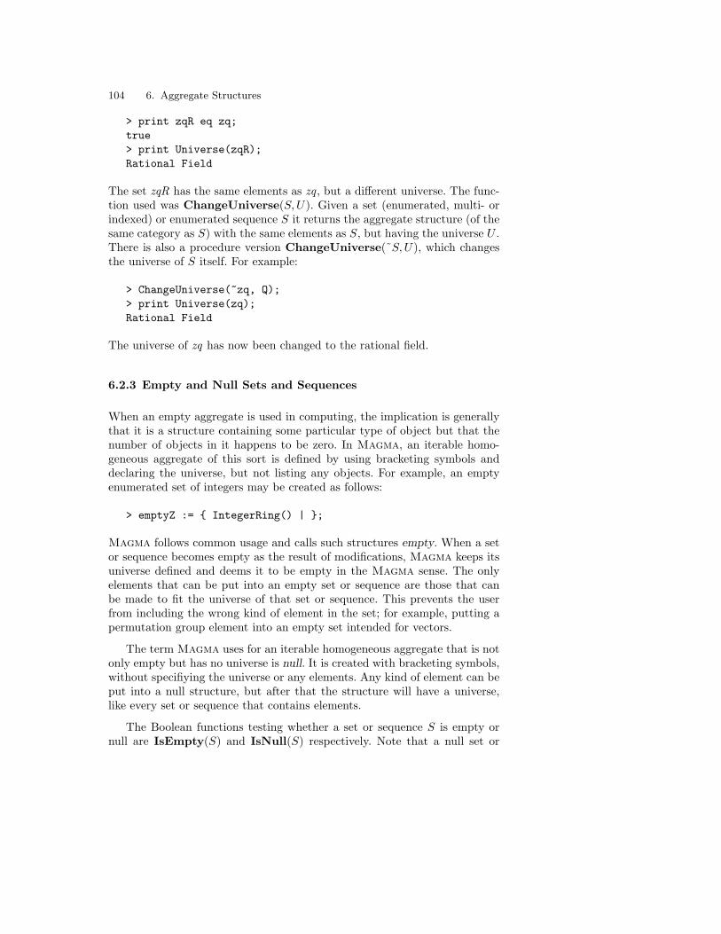
104 6. Aggregate Structures
> print zqR eq zq;true> print Universe(zqR);Rational Field
The set zqR has the same elements as zq , but a different universe. The func-tion used was ChangeUniverse(S,U). Given a set (enumerated, multi- orindexed) or enumerated sequence S it returns the aggregate structure (of thesame category as S) with the same elements as S, but having the universe U .There is also a procedure version ChangeUniverse(˜S, U), which changesthe universe of S itself. For example:
> ChangeUniverse(~zq, Q);> print Universe(zq);Rational Field
The universe of zq has now been changed to the rational field.
6.2.3 Empty and Null Sets and Sequences
When an empty aggregate is used in computing, the implication is generallythat it is a structure containing some particular type of object but that thenumber of objects in it happens to be zero. In Magma, an iterable homo-geneous aggregate of this sort is defined by using bracketing symbols anddeclaring the universe, but not listing any objects. For example, an emptyenumerated set of integers may be created as follows:
> emptyZ := IntegerRing() | ;
Magma follows common usage and calls such structures empty. When a setor sequence becomes empty as the result of modifications, Magma keeps itsuniverse defined and deems it to be empty in the Magma sense. The onlyelements that can be put into an empty set or sequence are those that canbe made to fit the universe of that set or sequence. This prevents the userfrom including the wrong kind of element in the set; for example, putting apermutation group element into an empty set intended for vectors.
The term Magma uses for an iterable homogeneous aggregate that is notonly empty but has no universe is null. It is created with bracketing symbols,without specifiying the universe or any elements. Any kind of element can beput into a null structure, but after that the structure will have a universe,like every set or sequence that contains elements.
The Boolean functions testing whether a set or sequence S is empty ornull are IsEmpty(S) and IsNull(S) respectively. Note that a null set or

6.2 Construction of Iterable Homogeneous Aggregates 105
sequence will return true when passed as an argument to IsEmpty, becauseit has no elements.
6.2.4 Construction of Arithmetic Progressions
Table 6.2. Enumerated sets and sequences from arithmetic progressions
Magma Meaning
i..j Set i, i + 1, . . . , j, where i, j ∈ ZZ
[i..j] Sequence [i, i + 1, . . . , j], where i, j ∈ ZZ
i..j by k Set i, i + k, i + 2k, . . . , j, where i, j, k ∈ ZZ, k 6= 0
[i..j by k] Sequence [i, i + k, i + 2k, . . . , j], where i, j, k ∈ ZZ, k 6= 0
Table 6.2 shows Magma’s special methods for constructing an enumer-ated set or enumerated sequence S whose elements are integers in arithmeticprogression. If the progression has common difference 1, then the syntaxi..j inside the bracketing symbol means the elements i, i + 1, i + 2, . . . , j.For example:
> TwentyToForty := 20..40;> print TwentyToForty; 20 .. 40
As the output implies, Magma stores the arithmetic progression rather thancomputing and storing all the elements. This is much more efficient if the car-dinality of S is large, and it is still possible during subsequent computationsto find elements or test whether an object is in S very quickly.
If the arithmetic progression has a common difference k other than 1, theappropriate syntax is i..j by k within bracketing symbols, meaning theprogression i, i+k, i+2k, . . . , j. If the progression is decreasing, then k shouldbe negative. (An empty structure results if i > j and k > 0 or if i < j andk < 0. If j is not of the form i+mk for some integer m, then the progressioncontinues as long as the range from i to j is not exceeded; that is, if k > 0 thelast element in the progression will be the greatest integer of the form i + nkthat is less than j, and if k < 0 the last element will be the least integer ofthe form i + nk that is greater than j.) For example:
> skip3 := [4..19 by 3]; seq2 := [87..43 by -2];> print skip3, seq2;[ 4 .. 19 by 3 ]

106 6. Aggregate Structures
[ 87 .. 43 by -2 ]
> skip3a := [4..21 by 3]; seq2a := [87..42 by -2];> print skip3 eq skip3a and seq2 eq seq2a;true
In an enumerated sequence created as an arithmetic progression, the firstelement is i, and the order of the elements proceeds along the progression.In an enumerated set, there is no true concept of order in the elements; inpractice, however, they are stored as increasing progressions (so that thedirection is changed if the common difference is negative), and iteration oversuch a set will occur in increasing order. The following example illustratesthis in the case of a for-statement (see Chapter 9):
> s := 9..3 by -2 ;> print s; 3 .. 9 by 2 > for x in s do> print x;> end for;3579
The arithmetic progression constructors are available only for enumeratedsets and enumerated sequences, not indexed sets or multisets. In the raresituation that an arithmetic progression has to be stored in one of thesestructures, a suitable transfer function (Table 6.9 (p. 146)) should be used:
> print SetToMultiset(s);* 3, 5, 7, 9 *> xs := SetToIndexedSet(4..8); print xs;@ 4, 5, 6, 7, 8 @
The universe of the result of an arithmetic progression constructor isalways the ring of integers, but aggregates with other universes may be con-structed from them, using the element-description method to be explainedbelow. For instance, the following expression returns the arithmetic sequenceof rational numbers ranging from zero to one and incrementing by tenths:
> print [x/10: x in [0..10]];[ 0, 1/10, 1/5, 3/10, 2/5, 1/2, 3/5, 7/10, 4/5, 9/10, 1 ]

6.2 Construction of Iterable Homogeneous Aggregates 107
6.2.5 Construction from an Element-Description
Another method of constructing an enumerated set, multiset, indexed set orenumerated sequence is to give an element-description, in a notation which isremarkably close to that of conventional mathematics. Magma calculates allthe elements of the aggregate from this description. The element-descriptionis made in terms of a general element, which is an expression in one ormore free identifiers xi. These free identifiers have local scope, and act as‘dummy variables’. Each identifier successively takes on the values of somefinite domain structure Ei, and certain combinations of the values of thefree identifiers are substituted into the expression for the general element.A domain Ei may be any iterable structure, that is, any iterable aggregateor any finite magma such that Magma can iterate over its elements (e.g., afinite field or a linear code).
As a preliminary example, the following line calculates the set consistingof the squares of the first five positive integers:
> squares := n^2 : n in [1..5] ;> print squares; 1, 4, 9, 16, 25
The expression for the general element is n^2, and the free identifier n rangesover the values 1,2,3,4,5, which are the elements of the domain structure[1..5]. Since free identifiers have local scope, their use in a constructor willnot interfere with an identifier of the same name outside the constructor. Forinstance:
> n := 91837410923;> squares := n^2 : n in [1..5] ;> print n;91837410923
The element-description aggregate constructor is enclosed in the appro-priate bracketing symbol for the relevant category of aggregate structure(enumerated set, multiset, indexed set or enumerated sequence). Immediatelyafter the opening bracket is an optional specification of the universe, consist-ing of an expression for the universe followed by the | symbol; however, itis less common to state the universe explicitly in this kind of constructionthan it is for element-list constructions.
The body of the constructor specifies the free identifiers and domains, anoptional Boolean condition indicating which elements of the domains are tobe used (all fo them being used if no condition is given), and an expressionin the free identifiers that is evaluated to find the elements of the aggregate.

108 6. Aggregate Structures
For simplicity, the body of the constructor will first be explained in the caseof a single free identifier x and domain E. It can take two forms, the simplerof these being:
expression : x in E
Here the expression is in the free identifier x. The elements of the resultingaggregate are the values of the expression in x, evaluated for all x ∈ E. Themore general syntax is:
expression : x in E | condition
Here the condition is also an expression in the free identifier x, but it mustevaluate to a Boolean. The elements of the aggregate are the values of theexpression in x, evaluated for all x ∈ E such that the condition evaluates totrue.
If there are several free identifiers xi ranging over domains Ei, then theexpression on the left and the optional condition on the right should beexpressions in the xi. The syntax remains the same except for the sectionbetween the : and | symbols, which becomes:
x1 in E1, . . . , xk in Ek
If two or more adjacent domains are equal (Es = Es+1 = · · · = Et), then theabbreviation xs, . . . , xt in Es may be made for xs in Es, . . . , xt in Et. In orderto evaluate the element-description when there are several free identifiers,Magma considers all the k-tuples < x1, . . . , xk > where xi ∈ Ei for all i. Ifthere is no condition on the right, Magma evaluates the expression for eachk-tuple, to yield the elements of the aggregate under construction. If there isa condition given, Magma substitutes each k-tuple into the condition, andfor all those k-tuples such that the condition evaluates to true, it evaluatesthe expression to find the elements of the aggregate.
For example, let mu be the set of five times all the units in the residueclass ring ZZ/12ZZ. This set might be described more formally as ‘the set offive times y, where y is in the ring ZZ/12ZZ, such that y is a unit’, or as5y : y ∈ ZZ/12ZZ | y is a unit. The Magma syntax is similar:
> mu := 5*y : y in ResidueClassRing(12) | IsUnit(y) ;> print mu; 11, 1, 5, 7 > print Universe(mu);Residue class ring of integers modulo 12

6.2 Construction of Iterable Homogeneous Aggregates 109
Observe that an automatic coercion takes place in the expression 5*y: theinteger 5 is coerced into the ring ZZ/12ZZ, to which y belongs.
As another example, the following line evaluates the expression x3−7x2+2for x = −2,−1, 0, 1, 2, 3, 4, and places the result in an enumerated sequence:
> vals := [ x^3 - 7*x^2 + 2: x in [-2..4] ];> print vals;[ -34, -6, 2, -4, -18, -34, -46 ]> print Universe(vals);Integer Ring
The universe of vals as created above is the integer ring, because the valuescalculated are integers. If the user wishes the sequence to have a differentuniverse, such as the real field, then this universe should be placed on theleft of the constructor:
> vals := [ RealField() | x^3 - 7*x^2 + 2: x in [-2..4] ];> print Universe(vals);Real Field
Note that if a universe is specified but there is an element that cannot becoerced into the universe, then Magma gives an error message. For example:
> seqC := [ Sqrt(t) : t in [5, 2, -4] ];> print seqC;[ 2.236067977499789696409173668722,1.414213562373095048801688724198,2.0000000000000000000000000000*i ]> print Universe(seqC);Complex Field>> seqC := [ RealField() | Sqrt(t) : t in [5, 2, -4] ];
>> seqC := [ RealField() | Sqrt(t) : t in [5, 2, -4] ];^
Runtime error in sequence construction:Can’t coerce element into the universe
It occasionally happens in an element-description constructor that thecondition and the expression used to calculate the elements contain a com-mon sub-expression. There is a special kind of where-construction providedfor such cases, to increase the efficiency and compactness of the code. Thewhere-construction should be placed immediately after the condition, butits scope will extend to the expression for the elements as well. For example,

110 6. Aggregate Structures
the set constructor below finds the values of n in the range 2 to 100 such thatφ(n) ≤ 6, and also stores these values of φ(n) with the corresponding valueof n. By employing the where-construction, the user can avoid recalculatingφ(n) for the successful values of n:
> phi_le_6 := <n, phi>: n in 2..100 |> phi le 6 where phi is EulerPhi(n);> print phi_le_6; <5, 4>, <7, 6>, <10, 4>, <18, 6>, <2, 1>, <6, 2>,<8, 4>, <4, 2>, <9, 6>, <12, 4>, <14, 6>, <3, 2>
Note that each element of this sequence is a tuple, a kind of aggregate whichis discussed in Section 6.10.
The next two examples are of constructors involving more than one freeidentifier. Firstly, the following print-statement prints the set of all multiplesof the basis elements of the 4-dimensional vector space over the finite fieldwith 3 elements:
> F := FiniteField(3);> V := VectorSpace(F, 4);> print k * b : b in Basis(V), k in F ;
(0 0 0 1),(0 0 0 2),(0 0 0 0),(1 0 0 0),(0 2 0 0),(0 1 0 0),(0 0 1 0),(2 0 0 0),(0 0 2 0)
If some of the domains are equal, then it is possible to abbreviate the con-structor. For instance, consider the problem of finding the set of elements ofthe form 4K where K + 1 is a square and K = s2 + t3 where s and t rangeover the finite field with 83 elements. The solution is:
> fs := 4*K : s, t in FiniteField(83) | IsSquare(K+1)> where K is s^2 + t^3 ;> print fs; 0, 44, 45, 3, 47, 5, 6, 7, 8, 12, 55, 13, 57, 59, 17, 60,61, 19, 64, 21, 65, 22, 66, 23, 24, 25, 26, 27, 71, 29, 73,74, 32, 33, 34, 77, 36, 79, 37, 80, 82, 40

6.2 Construction of Iterable Homogeneous Aggregates 111
If there are several free identifiers, the domain Ei may depend on anyof the free identifiers to its right (i.e., xi+1, . . . , xk). For example, supposethat the user wishes to construct the set of all the unordered triples (withrepetitions permitted) of integers from 0 to 20 that sum to 20. Since eachtriple is unordered and may have repeated elements, a multiset is the bestway to represent it. Two solutions are presented below: an intuitive approach,and a method that is more efficient because no element is generated morethan once. The output from the time command shows the difference:
> time tr20A := *a, b, 20-a-b* :> a in [0..20-b], b in [0..20] ;Time: 0.100> time tr20B := *a, b, 20-a-b* :> a in [b..((20-b) div 2)], b in [0..20];Time: 0.020> print tr20A eq tr20B;true> print tr20B;
* 11, 3, 6 *, * 1, 3, 16 *, * 2, 14, 4 *,* 4, 7, 9 *, * 12, 2, 6 *, * 1, 9, 10 *,* 1, 4, 15 *, * 2, 8, 10 *, * 0, 3, 17 *,* 0, 13, 7 *, * 2, 13, 5 *, * 4, 6, 10 *,* 6, 7^^2 *, * 11, 1, 8 *, * 0, 14, 6 *,* 2, 3, 15 *, * 0, 12, 8 *, * 6^^2, 8 *,* 3, 8, 9 *, * 1, 12, 7 *, * 0^^2, 20 *,* 0, 15, 5 *, * 1, 13, 6 *, * 0, 2, 18 *,* 11, 2, 7 *, * 12, 4^^2 *, * 0, 1, 19 *,* 5, 6, 9 *, * 3^^2, 14 *, * 1, 14, 5 *,* 11, 4, 5 *, * 0, 4, 16 *, * 1^^2, 18 *,* 0, 11, 9 *, * 5^^2, 10 *, * 2^^2, 16 *,* 3, 7, 10 *, * 2, 9^^2 *, * 13, 3, 4 *,* 1, 2, 17 *, * 12, 3, 5 *, * 4, 8^^2 *,* 5, 7, 8 *, * 0, 10^^2 *
Note, however, that it is often preferable to use a set constructor slightlyinefficiently, with some needless regeneration of elements (as for the firstsolution to this problem), if the user’s own time is being saved by describingthe objects in a straightforward, naive way.
The ordering of the elements of an enumerated sequence or indexed setthat is constructed from an element description corresponds to the order inwhich they are generated by the constructor. This order, in turn, dependson the order in which the domain structures Ei produce their elements as

112 6. Aggregate Structures
values for free identifiers in the iteration process. For each domain, if it is anenumerated sequence or indexed set, then its elements are produced in theobvious order, from first to last; otherwise, the order of iteration depends onthe way Magma represents the domain internally, and it is unwise to makeassumptions about it. Considering all the domains E1, . . . , Ek, the valuesfrom the domains on the right of the list vary more frequently than those onthe left, as the following example shows:
> print [<a,b,c> : a in [1..2], b in [3..4], c in [5..6]];[ <1, 3, 5>, <2, 3, 5>, <1, 4, 5>, <2, 4, 5>,<1, 3, 6>, <2, 3, 6>, <1, 4, 6>, <2, 4, 6> ]
6.2.6 Recursive Definition of Enumerated Sequences
Enumerated sequences may be created in a manner imitating the recursiveor inductive definitions encountered in mathematics. Within the constructor,the function Self(i) returns the value of the ith term of the sequence currentlyunder construction; this enables terms which have already been constructedto be used in the calculation of new terms. The function Self() returns thecurrent value of the sequence itself.
For example, the Fibonacci numbers may be defined as F1 = 1, F2 = 1,and Fn = Fn−1 + Fn−2 for n > 2. In Magma the corresponding sequencedefinition for the first 50 Fibonacci numbers is:
> F := [n in 1, 2 select 1 else Self(n-1) + Self(n-2) :> n in [1..50]];
Of course, in this particular example a recursive definition is not necessary,because Magma has a suitable intrinsic function Fibonacci(n):
> F := [Fibonacci(n): n in [1..50]];
The following sequence provides a trivial example of the Self() function:
> print [Self(): n in [1..3]];[
[],[
[]],[
[],[

6.2 Construction of Iterable Homogeneous Aggregates 113
[]]
]]
6.2.7 Enumerated Sequences with Undefined Terms
It is possible for Magma sequences to have undefined terms. Such sequencesare called incomplete. Their main use is for building a sequence gradually,out of index order. For example, suppose that the user wishes to create asequence q3 by starting with an empty integer sequence and then definingits 7th and 5th terms first:
> q3 := [IntegerRing() | ];> q3[7] := 45;> q3[5] := 69;> print q3;[ undef, undef, undef, undef, 69, undef, 45 ]
Each of the undefined terms is represented in the output by the keywordundef. This keyword is only used in output; it cannot be included in anexpression.
The Boolean function IsDefined(Q, i) returns true if and only if the ith
term of the sequence Q is defined, and the procedure Undefine(˜Q, i) causesthe ith term of Q to become undefined.
Notice that Magma’s incomplete sequences permit a sequence Q to beconstructed without being initialized to a fixed length beforehand. The cur-rent length of the sequence, #Q, is simply the index of the furthermostdefined term, and can become smaller or greater as terms are defined orundefined. The only initialization necessary is to assign to the identifier asequence with no terms. It may be defined as a null sequence rather thanan empty sequence if preferred, provided that when the first term is definedMagma is able to compute from it the correct universe for the sequence.
Most functions that take sequences as their arguments require that thesequences be complete. The function IsComplete(Q) tests if this is so. Thebest way to make an incomplete sequence complete is to iterate over it, sinceMagma ignores undefined terms whenever iterating over a sequence. For ex-ample, the following statement assigns to q4 a complete sequence containingthe defined terms of q3 in the same order:
> q4 := [n: n in q3];> print q4;
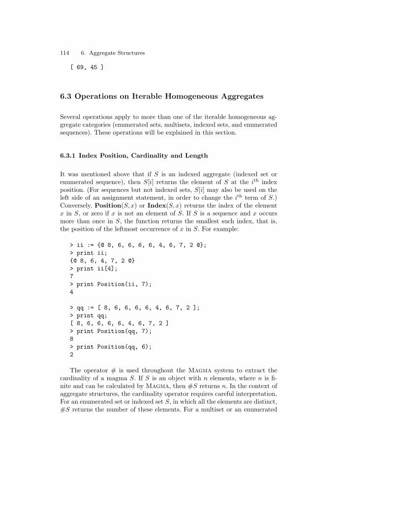
114 6. Aggregate Structures
[ 69, 45 ]
6.3 Operations on Iterable Homogeneous Aggregates
Several operations apply to more than one of the iterable homogeneous ag-gregate categories (enumerated sets, multisets, indexed sets, and enumeratedsequences). These operations will be explained in this section.
6.3.1 Index Position, Cardinality and Length
It was mentioned above that if S is an indexed aggregate (indexed set orenumerated sequence), then S[i] returns the element of S at the ith indexposition. (For sequences but not indexed sets, S[i] may also be used on theleft side of an assignment statement, in order to change the ith term of S.)Conversely, Position(S, x) or Index(S, x) returns the index of the elementx in S, or zero if x is not an element of S. If S is a sequence and x occursmore than once in S, the function returns the smallest such index, that is,the position of the leftmost occurrence of x in S. For example:
> ii := @ 8, 6, 6, 6, 6, 4, 6, 7, 2 @;> print ii;@ 8, 6, 4, 7, 2 @> print ii[4];7> print Position(ii, 7);4
> qq := [ 8, 6, 6, 6, 6, 4, 6, 7, 2 ];> print qq;[ 8, 6, 6, 6, 6, 4, 6, 7, 2 ]> print Position(qq, 7);8> print Position(qq, 6);2
The operator # is used throughout the Magma system to extract thecardinality of a magma S. If S is an object with n elements, where n is fi-nite and can be calculated by Magma, then #S returns n. In the context ofaggregate structures, the cardinality operator requires careful interpretation.For an enumerated set or indexed set S, in which all the elements are distinct,#S returns the number of these elements. For a multiset or an enumerated

6.3 Operations on Iterable Homogeneous Aggregates 115
sequence S, in which there may be more than one occurrence of the sameelement in S, #S returns the total number of elements, counting multiplici-ties. (However, for an enumerated sequence with undefined terms, it returnsthe highest position at which there is a defined term.) Notice that from thepoint of view of the indexed aggregates, this definition implies that #S isthe length or highest index of S; the same applies to #S where S is a string.Therefore S[#S] is the ‘last’ or rightmost element of S. For example:
> m := * wd[i]: i in [1..#wd] * where wd is "MISSISSIPPI";> print m;* M, I^^4, P^^2, S^^4 *> print #m;11
6.3.2 Testing Equality, Membership, and Subsetness
The relational operators eq (=) and ne ( 6=) may be applied to two aggre-gates R and S in the same category to test their equality/inequality. Theuniverses of R and S must be compatible, that is, they must either be equalor have a common overstructure into which elements of each aggregate canbe automatically coerced. In order for R eq S to return true, the elementsof R and S must be equal, counting multiplicities where that is relevant. Forinstance, the following two sets are regarded as equal by Magma, becausetheir elements are exactly equal after the integers in the set on the right arecoerced into the finite field:
> print FiniteField(7) | n: n in 2..5 eq 2..5;true
If R and S are equal then the order of their elements must be the same forenumerated sequences, but need not be the same for indexed sets. The reasonfor this is that order is an important aspect of the sequence concept, whereasindexed sets may be seen as modified enumerated sets with a convenientindexing facility.
The expressions x in S and x notin S are used to test whether a givenobject x is an element of (∈) an aggregate S (or a magma S). If the parentof x does not equal the universe of S, then Magma attempts auto-coercionof x into the universe before performing the membership test.
The expressions R subset S and R notsubset S compare two aggregates(or magmas) R and S to see whether R is a subset (⊆) of S, that is, whetherevery element of R is an element of S. Again, auto-coercion is attempted ifthe universes of R and S are not the same. The multiplicity of the elements

116 6. Aggregate Structures
is not relevant unless R and S are multisets, and the order of the elementsis never relevant. (If the two aggregates are both sequences, the functionIsSubsequence, explained on p. 122, performs a test that is similar butdoes consider the order of the elements.)
6.3.3 Including or Excluding an Element
The intrinsics Include and Exclude are used to place an element x in anaggregate S or take it from S. The parent of x must be compatible withthe universe of S. There are two versions: the functions Include(S, x) andExclude(S, x), which return a new aggregate but do not change the givenaggregate S, and the procedures Include(˜S, x) and Exclude(˜S, x), whichmodify S itself, as a reference argument. If the user wishes to change the valueof an existing aggregate, stored in an identifier, then the procedure versionshould be used; note that a procedure call is a statement by itself, and mustbe followed by a semicolon. (The ˜ symbol indicates that the identifier itprecedes is a variable reference argument, that is, an identifier whose valuethe procedure may change. See Section 8.3 for further discussion.)
The precise effect of these intrinsics depends on the category of S. IfS is an enumerated set then: the enumerated set computed by Include isS with x placed in it if x is not in S already, else S; the enumerated setcomputed by Exclude is S with x removed if x is in S, else S. If S is anindexed set then: the indexed set computed by Include is S with x placedat the end (in the index order) if x is not in S already, else S; the Excludeintrinsic does not exist for this category. If S is a multiset then: the multisetcomputed by Include is S with the multiplicity of x increased by 1, whetheror not S initially contains x; the multiset computed by Exclude is S withthe multiplicity of x decreased by 1, if x is in S, else S. Finally, if S is anenumerated sequence then: the enumerated sequence computed by Includeis S with x placed at the end (in the index order) if x is not in S already, elseS; the enumerated sequence computed by Exclude is S with the leftmostinstance of x removed (and the terms to the right of this moved one place tothe left) if x is in S, else S.
6.3.4 Maximum and Minimum Elements
The functions Maximum(S) and Minimum(S), which have abbreviationsMax(S) and Min(S), may be applied to an aggregate S whose universe hasa total ordering defined on its elements. (Examples are ordered rings, freegroups, semigroups and monoids, and the string monoid.) These functionsreturn the maximum or minimum element of S. If S is an enumerated se-quence or an indexed set, the functions have a second return value, namely

6.3 Operations on Iterable Homogeneous Aggregates 117
the index of the (leftmost) position where the maximal or minimal elementoccurs. A multiple assignment statement should be used to obtain both val-ues. (Another way to obtain both values is to invoke the function by itself asthe expression in a print-statement.)
6.3.5 Reduction
The operation of reduction takes an aggregate S and returns an object withthe same parent as the elements of S have. Assuming that is an associativebinary operator suitable for the universe of S, the expression & S returnsthe value of S1 S2 · · · Sn, where the Si are the elements of S, as describedon p. 98. Note that the Si may include repetitions, in the case of multisetsand enumerated sequences. If S is an enumerated sequence or indexed set,then the elements are taken in standard index order.
For example, the following statement evaluates∑10
i=1(i!)2, by performing
reduction using the addition operator on the sequence containing each (i!)2
for i = 1, . . . , 10:
> print &+[Factorial(i)^2: i in [1..10]];13301522971817
Similarly, consider the problem of finding the order of GL(n, GF(q)), that is,the number of non-singular n × n matrices over GF(q), where q is a primepower. It equals
n∏
i=1
(qn − qi−1)
so the Magma equivalent (assuming q and n have been assigned) is:
> ord := &*[q^n - q^(i-1) : i in [1..n]];
Finally, the following function, isperfect(n), applies reduction and sequenceoperations in order to test whether the integer argument n is a perfect number(i.e., whether n equals the sum of its divisors except for n itself):
> isperfect := func< n | n eq &+Exclude(Divisors(n), n) >;> print isperfect(6);true> print isperfect(7);false> print isperfect(28);true

118 6. Aggregate Structures
Any of the operators +, *, and, or, join and meet may be used to reducean aggregate provided that the operator is suitable for the universe. For se-quences containing sequences or strings, the associative but non-commutativeconcatenation operator cat is also available.
Aggregates with a cardinality of zero or one need special attention. Whenreduction is applied to an aggregate with cardinality one, the value returnedis the unique element of the aggregate. The special cases of reducing aggre-gates with no elements follow mathematical conventions for the operators.Summing or multiplying an empty aggregate returns 0 or 1 respectively, ifthe universe is suitable. On an empty aggregate of Booleans, or on a nullaggregate, &and returns true and &or returns false.
6.4 Further Operations on Set Categories
Besides the operations given in Section 6.3, there are further operations avail-able for the categories of enumerated sets, multisets and indexed sets.
The binary operations of union and intersection may be applied to twoaggregates R and S in the same set category, provided that their universesare compatible. The aggregate returned will have the same category as thecategory of the arguments. The expression R join S returns the aggregate R∪S, and R meet S returns R∩S. If R and S are indexed sets, no generalizationscan be made about the indexing of the result. If R and S are multisets, Rjoin S is constructed by adding multiplicities, and R meet S is constructedby taking the minimum of the multiplicities for each element. For example:
> print 3..9 by 2 join 1, 5, 11, 17 ; 1, 3, 5, 7, 9, 11, 17 > print * 1^^4, 3^^6, 8^^2 * join * 1, 2^^3, 8^^5 *;* 1^^5, 2^^3, 3^^6, 8^^7 *> print * 1^^4, 3^^6, 8^^2 * meet * 1, 2^^3, 8^^5 *;* 1, 8^^2 *
There are two other binary set operators that are available only for enu-merated sets and indexed sets, not for multisets. The expression R diff Sreturns the difference of R and S, that is, x : x ∈ R and x /∈ S, and theexpression R sdiff S returns the symmetric difference of R and S, that is,x : x ∈ R ∪ S and x /∈ R ∩ S. For example:
> print 3..9 by 2 diff 1, 5, 11, 17 ; 3, 7, 9 > print 3..9 by 2 sdiff 1, 5, 11, 17 ; 1, 3, 7, 9, 11, 17

6.4 Further Operations on Set Categories 119
These four set operators may also be used in mutation assignments. Forexample:
> FA3<a,b,c> := FreeAbelianGroup(3);> ix := @ a, b+c, 2*a-7*c @;> ix join:= @ 5*b, c @;> print ix;@
a,b + c,2*a - 7*c,5*b,c
@
For enumerated sets only, the procedure ExtractRep(˜R, ˜x) is pro-vided. Given an enumerated set R and an identifier x, it modifies R byextracting a representative element from it, and it assigns this element to x.For example:
> J := 15, 8, 13, 42, 20;> ExtractRep(~J, ~r);> print J, r; 8, 15, 20, 42 13
This procedure should not be confused with the function Rep(M), whichreturns a representative of the magma or aggregate M but does not changeM itself.
For enumerated sets only, there are several functions provided that con-struct subsets, sub-multisets, permutations, and so on. See Section 35.2for a full list. Perhaps the most generally applicable of these functions isSubsets(S, k). Given an enumerated set S and an integer k, it returns theset of all k-subsets of S, that is, all subsets of S having cardinality k. If k < 0or k > #S, the value returned is an empty set. For example:
> print Subsets(15, 8, 13, 42, 20, 2);
15, 42 , 8, 15 , 13, 42 , 8, 20 , 15, 20 , 13, 15 ,

120 6. Aggregate Structures
8, 13 , 13, 20 , 20, 42 , 8, 42
6.5 Further Operations on Enumerated Sequences
The operations in Section 6.3 apply to all the iterable homogeneous categoriesof aggregates, including enumerated sequences. This section discusses opera-tions that apply to enumerated sequences only; see Table 6.3 and Table 6.4for summaries. The operations in the first table are functions or operatorsthat return values; those in the second table mutate (change) the arguments,in a manner corresponding to the non-mutation versions. For efficiency, themutation operations should be employed where appropriate in preference tothe functional versions.
Table 6.3. Enumerated sequence operations returning values
Magma Meaning
Q cat T Sequence formed by chaining sequence T to end of se-quence Q: [q1, . . . , qn, t1, . . . , tm]
Position(Q, x),Index(Q, x)
Position of first occurrence of x in sequence Q, or zero ifno term in Q is x
Q[i] ith term of sequence Q
Q[I] [qi1 , . . . , qin ], where I is integer sequence [i1, . . . , in]
Q[i1, i2, . . . , ik] Q[i1][i2] . . . [ik] (multi-indexing)
Explode(Q) The terms of Q, in index order
Append(Q, x) Q with x placed on end
Prune(Q) Q with final term removed
Include(Q, x) Q with x placed on end, if x not in Q already
Exclude(Q, x) Q with first occurrence of x in Q deleted, if x in Q
Insert(Q, i, x) Q with x inserted at position i, and following elementsmoved along one place: [q1, . . . , qi−1, x, qi, . . . , qn]
Remove(Q, i) Q with ith term removed: [q1, . . . , qi−1, qi+1, . . . , qn]
Insert(Q, k, m, T ) Q with sequence T inserted, replacing terms qk throughto qm inclusive: [q1, . . . , qk−1, t1, . . . , tm, qm+1, . . . , qn]
Reverse(Q) Q with order of terms reversed
Rotate(Q, p) Q with terms rotated cyclically p terms to the right, or−p terms to the left if p negative
Sort(Q) Q with terms sorted into increasing order

6.5 Further Operations on Enumerated Sequences 121
Table 6.4. Enumerated sequence mutation operations
Q[i] := x Q cat := S
Append(˜Q, x) Prune(˜Q)
Include(˜Q, x) Exclude(˜Q, x)
Insert(˜Q, i, x) Remove(˜Q, i) Insert(˜Q, k, m, T )
Reverse(˜Q) Rotate(˜Q, p) Sort(˜Q)
6.5.1 Changing a Term of a Sequence
Let Q be an enumerated sequence. It has already been seen that the expres-sion Q[i] returns the ith term of Q, and that Position(Q, x) or Index(Q, x)returns the index of the leftmost occurrence of x in Q (or 0 if x is not in Q).It is possible to change Q at the ith term, by assigning a value to Q[i]. Forexample:
> fr := [x/10: x in [0..10]];> fr[6] := 99997;> print fr;[ 0, 1/10, 1/5, 3/10, 2/5, 99997, 3/5, 7/10, 4/5, 9/10, 1 ]
6.5.2 Obtaining Several Terms of a Sequence
The function Explode(Q) is a multiple return value function, operating ona sequence Q. Its return values are the terms Q[1], Q[2], . . . , Q[#Q], in thatorder. Thus the number of return values is dependent on the length of theargument. Explode is designed for situations where the user wishes to assignsome or all of a sequence’s terms to identifiers, without employing severalassignment statements.
Two examples of this function are given below. In the first example, allthe terms of the sequence [8, 7, 6] are assigned to identifiers. In the secondexample, only some of the terms of the sequence fr created above are assigned;see Section 3.3.3 for details of the multiple assignment statement and the _character as they are used here.
> z1, z2, z3 := Explode([8, 7, 6]);> print z1;8> print z2;7> print z3;6

122 6. Aggregate Structures
> first, second, _, _, fifth := Explode(fr);> print first;0> print second;1/10> print fifth;2/5
6.5.3 Subsequences and Concatenation
It is possible to form a new sequence by selecting several of the terms ofa sequence Q. The syntax for this operation is Q[I], where I is an integersequence containing the positions of the required terms. In the special casethat I is an arithmetic progression, the abbreviation Q[i..j by k] may bemade for the full form Q[[i..j by k]], and similarly Q[i..j] is an abbreviationfor Q[[i..j]]. For example:
> print fr[[1, 3, 7, 9]];[ 0, 1/5, 3/5, 4/5 ]> print fr[2..8 by 3];[ 1/10, 2/5, 7/10 ]
However, Q[I] may not be placed on the left of an assignment statement inorder to reassign several terms of a sequence simultaneously.
The expression Q cat T returns the concatenation of the enumeratedsequences Q and T , that is, the sequence [Q[1], . . . , Q[#Q], T [1], . . . , T [#T ]].For example:
> q1 := [4, 8/3, 7/10, 33, 2, 1/2];> q2 := q1 cat [-3/7, 8/3, 70, -5];> print q2;[ 4, 8/3, 7/10, 33, 19, 1/2, -3/7, 8/3, 70, -5 ]
If the user wishes to modify Q by concatenating T to it, then a mutationassignment with the operator cat:= should be used:
> qq := [5..9];> qq cat:= [100..400 by 100];> print qq;[ 5, 6, 7, 8, 9, 100, 200, 300, 400 ]
Given enumerated sequences Q and T , the function IsSubsequence(Q,T )returns true if Q is a subsequence of T . This function has three ways of in-
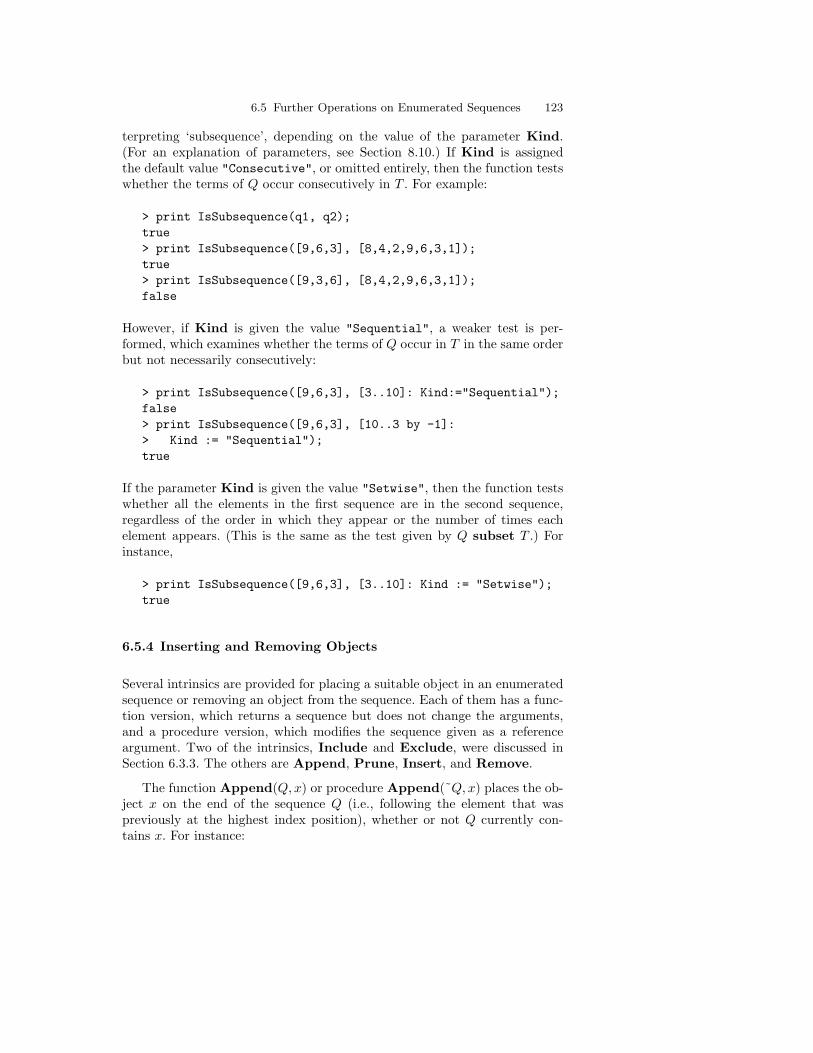
6.5 Further Operations on Enumerated Sequences 123
terpreting ‘subsequence’, depending on the value of the parameter Kind.(For an explanation of parameters, see Section 8.10.) If Kind is assignedthe default value "Consecutive", or omitted entirely, then the function testswhether the terms of Q occur consecutively in T . For example:
> print IsSubsequence(q1, q2);true> print IsSubsequence([9,6,3], [8,4,2,9,6,3,1]);true> print IsSubsequence([9,3,6], [8,4,2,9,6,3,1]);false
However, if Kind is given the value "Sequential", a weaker test is per-formed, which examines whether the terms of Q occur in T in the same orderbut not necessarily consecutively:
> print IsSubsequence([9,6,3], [3..10]: Kind:="Sequential");false> print IsSubsequence([9,6,3], [10..3 by -1]:> Kind := "Sequential");true
If the parameter Kind is given the value "Setwise", then the function testswhether all the elements in the first sequence are in the second sequence,regardless of the order in which they appear or the number of times eachelement appears. (This is the same as the test given by Q subset T .) Forinstance,
> print IsSubsequence([9,6,3], [3..10]: Kind := "Setwise");true
6.5.4 Inserting and Removing Objects
Several intrinsics are provided for placing a suitable object in an enumeratedsequence or removing an object from the sequence. Each of them has a func-tion version, which returns a sequence but does not change the arguments,and a procedure version, which modifies the sequence given as a referenceargument. Two of the intrinsics, Include and Exclude, were discussed inSection 6.3.3. The others are Append, Prune, Insert, and Remove.
The function Append(Q, x) or procedure Append(˜Q, x) places the ob-ject x on the end of the sequence Q (i.e., following the element that waspreviously at the highest index position), whether or not Q currently con-tains x. For instance:

124 6. Aggregate Structures
> Append(~q2, 99);> print q2;[ 4, 8/3, 7/10, 33, 2, 1/2, -3/7, 8/3, 70, -5, 99 ]> Append(~q2, 70);> print q2;[ 4, 8/3, 7/10, 33, 2, 1/2, -3/7, 8/3, 70, -5, 99, 70 ]
The function Prune(Q) and the procedure Prune(˜Q) are used to removethe last term from the sequence Q. For instance:
> print Prune(q2);[ 4, 8/3, 7/10, 33, 2, 1/2, -3/7, 8/3, 70, -5, 99 ]
Another way of inserting and removing terms of a sequence is by specifyingthe sequence position which is to be affected. The relevant intrinsics areInsert(Q, i, x) or Insert(˜Q, i, x), which inserts x at the ith position of Qand moves along the rest of the sequence to make room, and Remove(Q, i)or Remove(˜Q, i), which removes the ith term from Q and moves back therest of the sequence to fill the gap. For instance:
> q3 := Insert(q2, 4, 999);> print q3;[ 4, 8/3, 7/10, 999, 33, 2, 1/2, -3/7, 8/3, 70, -5, 99, 70 ]> print Remove(q3, 4) eq q2;true
There is also a function Insert(Q, k, m, T ) or procedure Insert(˜Q, k, m, T )which inserts a sequence T into Q, replacing terms Q[k] through to Q[m]inclusive. If the user does not wish to destroy any of the terms of Q, butmerely to place T after the mth term of Q and then continue with the restof Q, then k should be set at (m + 1).
6.5.5 Rearranging the Terms of a Sequence
There are three intrinsics that change the order of the terms of an enumer-ated sequence Q. Again, each has a function version and a procedure version.The enumerated sequence constructed by Reverse(Q) or Reverse(˜Q) isQ with its terms in reverse order, that is, [Q[#Q], . . . , Q[1]]. The functionRotate(Q, p) or procedure Rotate(˜Q, p) has the effect of rotating the termsof Q cyclically p terms to the right. If p ≥ 0, the result is Q[(n − p + 1)..n]concatenated with Q[1..(n−p)], and if p < 0, the result is Q[(−p+1)..n] con-catenated with Q[1..−p], where n = #Q. The result of Sort(Q) or Sort(˜Q)is Q with its terms sorted into increasing order; this intrinsic is only availableif the universe of Q has a total ordering defined on its elements. For example:

6.5 Further Operations on Enumerated Sequences 125
> y := [10..20]; y_copy := y;> Rotate(~y, 3);> print y;[ 18, 19, 20, 10, 11, 12, 13, 14, 15, 16, 17 ]> print Reverse(y);[ 17, 16, 15, 14, 13, 12, 11, 10, 20, 19, 18 ]> print Sort(y) eq y_copy;true
6.5.6 Multi-Dimensional Sequences
The elements of a set or sequence may themselves be sets or sequences, andthe nesting may occur to arbitrary depth (within memory limits). In thecase of sequences, this property permits the creation of multi-dimensional‘arrays’. Magma has a multi-index facility, whereby a comma-separated listof index positions may be placed within square brackets in order to specifythe coordinates of a sequence entry. The multi-index allows the user to reacheasily into inner levels of the sequence. In fact, multi-indexing may be appliedto any combination of sequences, lists, and tuples.
For example, consider the following sequence Q of sequences of integers.Top-level (standard) terms of Q may be extracted in the usual manner:
> Q := [ [40,50], [77,66,55], [], [150,250,350,450] ];> print Q;[
[ 40, 50 ],[ 77, 66, 55 ],[],[ 150, 250, 350, 450 ]
]
> print Q[2];[ 77, 66, 55 ]
However, each term of Q is a sequence, and so terms of these sequencesmay also be extracted. There are two ways to perform this operation. Firstly,the inner term may be described as a term of a term of Q, using the notationQ[i][j]. Secondly, the indices may be abbreviated into a multi-index, usingthe notation Q[i, j]. For example:
> print Q[2][3];55

126 6. Aggregate Structures
> print Q[2, 3];55
6.6 Representative and Random Elements
As is explained on p. 84, the function Rep(M) returns a representative el-ement of M , for most finite magmas M . For iterable magmas E, there isan alternative which is preferable because it is more efficient in regard tocomputer time and storage. It is the rep-constructor, whose syntax is closelybased on that for the homogeneous iterable aggregate constructors:
rep x : x in E | condition
where the Boolean condition is expressed in terms of x. When Magma eval-uates this constructor, it begins to loop through the elements of E. It returnsthe first element x that satisfies the condition. In this way, Magma avoidsbuilding the whole set x : x in E | condition, which might consume a greatdeal of resources.
For example, consider the problem of finding an odd permutation in thesymmetric group of degree 5:
> print repg: g in Sym(5) | IsOdd(g);(2, 3)
Magma returns the first suitable group element it finds, in this case (2, 3).
Obtaining a random element follows a similar process to obtaining a rep-resentative element. Instead of employing the function Random(M), theuser can apply the random-constructor:
random x : x in E | condition
Given this constructor, Magma will return a random element x of E satis-fying the condition. For instance, the following lines construct some randomelements of the permutation group on six elements which are not in the cyclicgroup on six elements:
> S6 := Sym(6);> C6 := CyclicGroup(GrpPerm, 6);> print randomg: g in S6 | g notin C6;(3, 5, 4, 6)> print randomg: g in S6 | g notin C6;

6.7 Existential and Universal Quantifiers 127
(1, 4, 6, 2, 3)> print randomg: g in S6 | g notin C6;(1, 4, 3, 5, 2, 6)
The constructors rep and random are also available in a multi-identifierversion, following the syntax for element-description constructors.
If the set specified in a rep or random constructor is empty, so that therecan be no representative element, then Magma will give an error message.In cases where the user is unsure whether there is an element satisfying thecondition, the quantifier exists should be employed, as explained in the nextsection.
6.7 Existential and Universal Quantifiers
There are two Magma constructors that are related to the mathematicalnotions of ‘there exists’ (∃) and ‘for all’ (∀). Their syntax is similar to thesyntax of the rep and random constructors:
exists x : x in E | condition forall x : x in E | condition
where E is an iterable magma. Each of these constructors returns a booleanvalue: exists returns true if the set described in the constructor is non-empty,else false; and forall returns true if the set described in the constructor isequal to E, else false. However, these constructors do not always build thewhole set before returning a value. Instead, they iterate over E, testing thecondition for each x in E, and they stop the iteration as soon as the returnvalue is known, which may be long before every element of E has been tested.
For example, let S5 be the symmetric group on six elements and let SLbe the subgroup lattice of S5 . The following lines verify that the order ofeach subgroup divides the order of S5 :
> S5 := Sym(5);> ordS5 := Order(S5);> SL := SubgroupLattice(S5);> print forallsg : sg in SL | IsZero(ordS5 mod Order(sg));true
Suppose now that the user wishes to know whether there are any perfectnumbers in the range 100 to 10000. This may be done using the exists-constructor and the function isperfect(n) discussed on p. 117:

128 6. Aggregate Structures
> isperfect := func< n | n eq &+Exclude(Divisors(n), n) >;> print exists n : n in [100..10000] | isperfect(n) ;true
The output shows that there exists at least one perfect number in that range.Magma stops iterating over the sequence as soon as one perfect number isfound, so the time taken is much less than the time taken to examine everyelement in the sequence:
> time print exists n : n in [100..10000] | isperfect(n) ;trueTime: 1.390> time print n : n in [100..10000] | isperfect(n) ; 496, 8128 Time: 66.066
The exists and forall constructors always return a boolean value. How-ever, if the constructors are used in a modified syntax then they can returnan element of the iterable magma E as well, under certain conditions. Thesyntax required is:
exists(d) x : x in E | condition forall(d) x : x in E | condition
where d is an identifier. If exists returns true, then d will be assigned an ele-ment of E that satisfies the condition; if it returns false, then d remains unas-signed (or becomes unassigned). As for the forall-constructor, if it returnsfalse, then d will be assigned an element of E that does not satisfy the con-dition (i.e., a counter-example); if it returns true, then d remains/becomesunassigned. For example:
> print exists(N) n : n in [100..10000] | isperfect(n) ;true> print N;496> print forall(k) n : n in [100..10000] | isperfect(n) ;false> print k;100
The exists and forall constructors may also be applied to situations in-volving more than one free identifier and domain, in a manner correspondingto that for the aggregate constructors. For example, let D6 be the dihe-dral group D6 under the permutation representation. The following exists-

6.8 Creating and Operating on Formal Sets 129
constructor tests whether there are elements p and q of orders 3 and 2 whichcommute, and finds an instance of such elements:
> D6 := DihedralGroup(GrpPerm, 6);> print exists(pair)<p, q>: p, q in D6 | p*q eq q*p and> Order(p) eq 3 and Order(q) eq 2;true> print pair;<(1, 3, 5)(2, 4, 6), (1, 4)(2, 5)(3, 6)>> print (pair[1], pair[2]); // commutator operator (a, b)Id(D6)
The components of the tuple pair satisfy the given condition.
6.8 Creating and Operating on Formal Sets
A formal set F is a subset of a magma M , described as those elementsof M that satisfy some boolean condition. F is represented internally interms of M and the condition, not by storing a collection of elements. Unlikethe aggregates discussed so far in this chapter, formal sets may be infinite.However, they only have a limited number of operations; for example, itis possible to test whether a given object is in a formal set F , but not toobtain elements of F from F itself. Formal sets are used in such contexts asspecifying the domain or codomain of a mapping, or giving the parent for arecord field.
The constructor for a formal set has the general form
! x in M | condition !,
where M is any (not necessarily iterable) magma for which it is possible totest membership of objects in M , and the condition is a boolean expressionin the free identifier x. The elements of this set are those elements of Mthat satisfy the condition, and the universe of the set is M . The versionof this constructor without the condition, ! x in M !, is the same asFormalSet(M), and may be considered as the formal carrier set of M .
For instance, the following statements create the formal set Zplus of pos-itive integers and the formal set Qd7 of rationals whose denominator (aftercancellation) is 7:
> Zplus := ! n in IntegerRing() | n gt 0 !;> print Zplus;

130 6. Aggregate Structures
Formal set over Integer Ring
> Qd7 := ! r in RationalField() | Denominator(r) eq 7 !;> print Qd7;Formal set over Rational Field> print Universe(Qd7);Rational Field
The great advantage of formal sets is that they can be infinite; the dis-advantage is that only a small number of operations are available for them.The binary set operations join, meet, diff, and sdiff, as explained on p. 118,may be applied if the two formal sets are compatible, and are implementedusing boolean operations on the conditions. The operators in and notin testwhether the given object (of a suitable kind) is an element of the given formalset. For example:
> print 42 in Zplus, 0 in Zplus, -3 in Zplus;true false false> print 8/7 in Qd7, 21/7 in Qd7;true false> print 21/7 in Zplus join Qd7;true
Although the operations on them may seem restrictive, formal sets can bevery useful in combination with other Magma constructions because theypromote the writing of succinct and lucid code.
6.9 Lists
The purpose of the category List is to give the user a means to collecttogether several objects of assorted kinds. This would generally be done asa temporary measure during a larger task. Aggregates in this category arecalled lists, but this is a technical usage of the word, not to be confused withthe informal use of ‘list’ elsewhere in this book.
Lists are ordered, iterable, and capable of containing repeated elements.However, their elements do not have to belong to the same magma, or even thesame category. Therefore lists are like enumerated sequences, except withoutthe restriction of homogeneity; the list bracket [* is intended to suggest this,by its similarity to the plain bracket [ for enumerated sequences. However,enumerated sequences have more operations than lists and are much moreefficient, so they should be preferred to lists whenever possible.

6.9 Lists 131
Table 6.5. Operations on lists
Magma Meaning
#L Length of list L (number of elements)
IsEmpty(L) true if L is empty (has zero length)
L[i] ith term of list L (1 ≤ i ≤ #L)
L[i] := x Changes L by assigning x to the ith term (1 ≤ i ≤ #L + 1)
L[i1, i2, . . . , ik] L[i1][i2] . . . [ik] (multi-indexing)
L cat K List formed by chaining list K to end of list L
L cat := K Changes L to (L cat K)
Append(L, x) L with x placed on end
Append(˜L, x) Changes L to L with x placed on end
Prune(L) L with final term removed
Prune(˜L) Changes L to L with final term removed
The only way to create a list is to ‘list’ its elements within the symbols[* and *], since the more sophisticated constructors are not available. Forexample:
> L := [* GF(8), "r", 1/3 *];> print L;[* Finite field of size 2^3, r, 1/3 *]> print Category(L);List
The operations on lists, shown in Table 6.5, are an abridged version of theoperations on enumerated sequences. The principal operations are finding thelength of a list, accessing and changing the ith term, concatenation, appendingand pruning. For example:
> print #L;3> L[2] := KCubeGraph(2);> Append(~L, ReedMullerCode(2, 3));
> print L;[* Finite field of size 2^3,GraphVertex Neighbours
1 2 3 ;2 1 4 ;3 1 4 ;

132 6. Aggregate Structures
4 2 3 ;, 1/3, [8, 7, 2] Reed-Muller Code (r = 2, m = 3) over GF(2)Generator matrix:[1 0 0 0 0 0 0 1][0 1 0 0 0 0 0 1][0 0 1 0 0 0 0 1][0 0 0 1 0 0 0 1][0 0 0 0 1 0 0 1][0 0 0 0 0 1 0 1][0 0 0 0 0 0 1 1] *]
6.10 Cartesian Products and Tuples
Table 6.6. Cartesian products
Magma Meaning
car< M1, . . . , Mk > Cartesian product M1 × · · · ×Mk
CartesianProduct(M, N) M ×N
CartesianPower(M, k) M × · · · ×M (k components)
Flat(C) Given Cartesian product C whose compo-nents may include Cartesian products, returnCartesian product of the base structures, con-sidered in depth-first order
NumberOfComponents(C) Number k of components of C
C eq D true if corresponding components of C andD are equal
Rep(C) Representative element of C
#C Cardinality of finite C
Set(C) Set of elements of finite C
Random(C) Random element of finite C
Given the magmas (or aggregates) M1, . . . , Mk, the Cartesian productC = M1 × · · · ×Mk of these magmas is a kind of set. Its elements or tuplesare of the form < m1, . . . , mk >, where each entry mi is an element of thecorresponding magma Mi. In Magma, a Cartesian product is created bylisting the component magmas in the product and surrounding them withthe bracketing symbols car< and >:
car< M1, . . . , Mk >
The category of Cartesian products is SetCart. Table 6.6 lists the functionsfor the creation and access of Cartesian products.
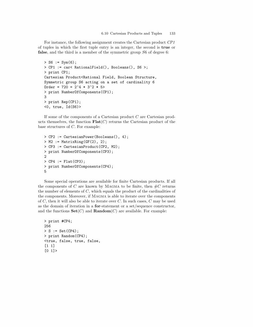
6.10 Cartesian Products and Tuples 133
For instance, the following assignment creates the Cartesian product CP1of tuples in which the first tuple entry is an integer, the second is true orfalse, and the third is a member of the symmetric group S6 of degree 6:
> S6 := Sym(6);> CP1 := car< RationalField(), Booleans(), S6 >;> print CP1;Cartesian Product<Rational Field, Boolean Structure,Symmetric group S6 acting on a set of cardinality 6Order = 720 = 2^4 * 3^2 * 5>> print NumberOfComponents(CP1);3> print Rep(CP1);<0, true, Id(S6)>
If some of the components of a Cartesian product C are Cartesian prod-ucts themselves, the function Flat(C) returns the Cartesian product of thebase structures of C. For example:
> CP2 := CartesianPower(Booleans(), 4);> M2 := MatrixRing(GF(2), 2);> CP3 := CartesianProduct(CP2, M2);> print NumberOfComponents(CP3);2> CP4 := Flat(CP3);> print NumberOfComponents(CP4);5
Some special operations are available for finite Cartesian products. If allthe components of C are known by Magma to be finite, then #C returnsthe number of elements of C, which equals the product of the cardinalities ofthe components. Moreover, if Magma is able to iterate over the componentsof C, then it will also be able to iterate over C. In such cases, C may be usedas the domain of iteration in a for-statement or a set/sequence constructor,and the functions Set(C) and Random(C) are available. For example:
> print #CP4;256> S := Set(CP4);> print Random(CP4);<true, false, true, false,[1 1][0 1]>

134 6. Aggregate Structures
Tuples, the elements of Cartesian products, may be created in severalways. The elt-constructor
elt< C | m1, . . . ,mk >
returns the tuple < m1, . . . , mk > as an element of the Cartesian product C.For example:
> t1 := elt< CP1 | 3, true, S6!(2, 4)(3, 6) >;> print t1;<3, true, (2, 4)(3, 6)>> print Parent(t1) eq CP1;true
Alternatively, if t already exists (as a tuple in a related Cartesian product),then it may be coerced into C by means of the coercion operation C!t.
It is also possible to create a tuple without specifying its parent explicitly.This is a common method in Magma programming; see p. 110 above for anexample. The tuple constructor
< m1, . . . ,mk >
returns the tuple < m1, . . . ,mk > as an element of the Cartesian product ofthe parents of the mi. In other words, Magma deduces the parent productfrom the entries of the tuple. For instance:
> t2 := < 3, true, S6!(2, 4)(3, 6) >;> print Parent(t2) eq CP1;false> print Parent(t2);Cartesian Product<Integer Ring, Boolean Structure,Symmetric group S6 acting on a set of cardinality 6Order = 720 = 2^4 * 3^2 * 5>
Table 6.7 lists the operations on tuples; notice that they resemble thesequence operations to some extent. The indexing operations are restrictedby the fact that once a tuple t has been created, its parent C is fixed, andany subsequent mutations of t have to conform to C. Therefore the numberof entries of t cannot change, and any new value for an entry must have theappropriate parent. For example, the first components of the parents of t1and t2 are Q and ZZ respectively, so t1[1] may be changed to a non-integralrational but t2[1] may not:
> t1[1] := 17/23;

6.10 Cartesian Products and Tuples 135
Table 6.7. Tuples
Magma Meaning
elt< C | m1, . . . , mk > Tuple < m1, . . . , mk > as element of C
< m1, . . . , mk > Tuple < m1, . . . , mk > as element of Cartesian prod-uct implied by the parents of the mi
C!t Element of C corresponding to tuple t (entries of tmust be coercible into components of C)
Parent(t) Cartesian product to which tuple t belongs
t in C true if tuple t is an element of C
t eq u true if corresponding entries of t and u are equal
#t Number of entries of tuple t
t[i] ith entry of tuple t
t[i1, i2, . . . , ik] t[i1][i2] . . . [ik] (multi-indexing)
Explode(t) All entries of t, in order (multiple return value)
> print t1;<17/23, true, (2, 4)(3, 6)>> t2[1] := 17/23;
>> t2[1] := 17/23;^
Runtime error in :=: New component not in cartesian product
It is not possible to iterate directly over a tuple t, but this may be achievedindirectly by iterating over its index:
> for i in [1..#t1] do> print t1[i];> end for;17/23true(2, 4)(3, 6)
Given a tuple t, the function Explode(t) returns all its entries separately,in their index order. The purpose of this function is to provide a simple meansof assigning tuple entries to identifiers, without having to use the notationt[i] several times. For example:
> ratl, bl, g := Explode(t1);> print ratl;17/23> print bl;true

136 6. Aggregate Structures
> print g;(2, 4)(3, 6)
The main purpose of tuples, when considered in their own right ratherthan as elements of Cartesian products, is to collect together related butinhomogeneous information. Several of Magma’s functions return tuples forthis reason. For instance, if the integer polynomial x4 + 5x3 + 10x2 + 96x +288 is given as an argument to the function Factorization, the output isa factorization sequence of 2-tuples whose first entry is a factor and whosesecond entry is the multiplicity of that factor:
> P<x> := PolynomialAlgebra(IntegerRing());> f := Factorization(x^4 + 5*x^3 + 10*x^2 + 96*x + 288);> print f;[
<x + 4, 2>,<x^2 - 3*x + 18, 1>
]> print Universe(f);Cartesian Product<Univariate Polynomial Algebra in xover Integer Ring, Integer Ring>
Individual factors may be extracted by sequence and tuple manipulation.For instance, the second factor may be obtained as follows, since f [2] is thesecond tuple and its first entry is the factor:
> factor2 := f[2][1];> print factor2;x^2 - 3*x + 18> // or a multi-index:> print f[2, 1];x^2 - 3*x + 18
6.11 Coproducts
Coproducts, which are the duals of Cartesian products, provide a means todraw together the elements of several magmas or aggregates S1, . . . , Sn intoa single structure C. The Si are called the constituents of C. Each elementx of C arises from exactly one of the constituents, and although x has C asits parent, there is a way of determining which Si is the original parent of x.The coproduct functions include a universal map facility.
The constructor for the coproduct of S1, . . . , Sn is

6.11 Coproducts 137
cop< S1, . . . , Sn >
However, if the constituents have been placed into a sequence Q then thefollowing alternative form may be used:
cop< Q >
This constructor returns the coproduct C as its principal return value, butalso returns a sequence of maps [m1,m2, ..., mk]. These maps are the injec-tions mi : Si → C that define the coproduct. (This sequence of maps is alsoavailable from the function Injections(C).) The examples below illustratethe two versions of the coproduct constructor:
> F25 := FiniteField(5, 2);> C, m := cop< F25, Strings(), IntegerRing() >;> print C;Coproduct<Finite field of size 5^2, String structure,Integer Ring>> print m;[
Mapping from: FldFin: F25 to Cop: C,Mapping from: String structure to Cop: C,Mapping from: Integer Ring to Cop: C
]
> q := [ FiniteField(p) : p in [1..20] | IsPrime(p) ];> CC, mm := cop< q >;> print CC, mm;Coproduct<Finite field of size 2, Finite field of size 3,Finite field of size 5, Finite field of size 7,Finite field of size 11, Finite field of size 13,Finite field of size 17, Finite field of size 19>[
Mapping from: GF(2) to Cop: CC,Mapping from: GF(3) to Cop: CC,Mapping from: GF(5) to Cop: CC,Mapping from: GF(7) to Cop: CC,Mapping from: GF(11) to Cop: CC,Mapping from: GF(13) to Cop: CC,Mapping from: GF(17) to Cop: CC,Mapping from: GF(19) to Cop: CC
]
The function Constituent(C, i) returns the ith constituent of the coproductC, and #C returns the number of constituents.

138 6. Aggregate Structures
Given s ∈ Si, there is a corresponding element x ∈ C given by the injec-tion mi. To create x in Magma, the most general method is to apply thisinjection, using the standard syntax for mappings, as explained in Chapter7:
> s := F25 ! 3;> print Parent(s);Finite field of size 5^2
> x1 := m[1](s);> print x1;3> print Parent(x1);Coproduct<Finite field of size 5^2, String structure,Integer Ring>
> xx := mm[6]( Random(Constituent(CC, 6)) );> print xx;11
However, if the category of Si is unique in the coproduct, then coercion usingthe ! operator is an alternative method:
> x2 := C ! s;> print x1 eq x2;true
Once an element x of C has been created, as the image of si ∈ Si, theparent of x will be C. However, sufficient information is stored with x forthe corresponding si and Si to be reconstructed. The function Index(x)returns the constituent number i, and Si may then be found from the func-tion Constituent(C, i). Moreover, the function Retrieve(x) returns si. Forexample:
> print Index(x1);1> print Constituent(C, 1);Finite field of size 5^2
> rtv := Retrieve(x1);> print Parent(rtv) eq F25 and rtv eq s;true
> print Parent(Retrieve(xx));Finite field of size 13

6.11 Coproducts 139
If the constituents of a coproduct C include one or more structures thatare themselves coproducts, then the function Flat(C) may be used to findthe corresponding coproduct of the base structures, considered in depth-firstorder. For example, CCC is created below as the coproduct of C and CC ,and then it is flattened so that its constituents are the constituents of C andCC :
> CCC, mmm := cop< C, CC >;> print CCC, mmm;Coproduct<Coproduct<Finite field of size 5^2,String structure, Integer Ring>,Coproduct<Finite field of size 2, Finite field of size 3,Finite field of size 5, Finite field of size 7,Finite field of size 11, Finite field of size 13,Finite field of size 17, Finite field of size 19>>[
Mapping from: Cop: C to Cop: CCC,Mapping from: Cop: CC to Cop: CCC
]
> fCCC, fmmm := Flat(CCC);> print fCCC, fmmm;Coproduct<Finite field of size 5^2, String structure,Integer Ring, Finite field of size 2,Finite field of size 3, Finite field of size 5,Finite field of size 7, Finite field of size 11,Finite field of size 13, Finite field of size 17,Finite field of size 19>[
Mapping from: FldFin: F25 to Cop: fCCC,Mapping from: String structure to Cop: fCCC,Mapping from: Integer Ring to Cop: fCCC,Mapping from: GF(2) to Cop: fCCC,Mapping from: GF(3) to Cop: fCCC,Mapping from: GF(5) to Cop: fCCC,Mapping from: GF(7) to Cop: fCCC,Mapping from: GF(11) to Cop: fCCC,Mapping from: GF(13) to Cop: fCCC,Mapping from: GF(17) to Cop: fCCC,Mapping from: GF(19) to Cop: fCCC
]
Finally, the function UniversalMap(C, D, Q) returns the universal mapfrom the coproduct C to the structure D. The third argument of this func-tion is a sequence Q of maps Si → D, where the Si are the constituents of

140 6. Aggregate Structures
D. Magma uses these maps to calculate the universal map. For example,suppose that D is the boolean structure, and that the original coproduct isthe coproduct CC above, whose constituents are the finite fields q[i]. To keepthe example simple, let each of the maps q[i] → D be of the same generalkind, namely, a test of the primitivity of the given finite field element. Theresult is:
> D := Booleans();> qq := [ map< gf -> D | f :-> IsPrimitive(f) > : gf in q ];> um := UniversalMap(CC, D, qq);> print um;Mapping from: Cop: CC to Bool: Bgiven by function(x) ... end function> print um(xx);true
The output in the final line may be interpreted as saying that the constituentelement corresponding to xx (that is, the element 11 in the finite field with13 elements) is a primitive element of its field.
Table 6.8. Operations on coproducts
Magma Meaning
#C Number of constituents of coproduct C
Injections(C) Sequence [m1, . . . , m#C ] of injections from con-stituents into C (same as the second return valueof the cop-constructor)
Constituent(C, i) ith constituent of C
Index(x) Constituent number i of x ∈ C
Retrieve(x) Element si of constituent Si such that mi(si) = x
Flat(C) Flattened coproduct corresponding to C, where Cis a coproduct of coproducts
UniversalMap(C, D, Q) Given coproduct C with constituents Si, structureD, and sequence Q of maps Si → D, returns uni-versal map C → D
Table 6.8 summarizes the operations on coproducts. Note that there is noequality test between coproducts, since this is not feasible in general.

6.12 Record Formats and Records 141
6.12 Record Formats and Records
6.12.1 Creating Record Formats and Records
The most noticeable difference between records and tuples is that the fieldsof a record have names, whereas the components of a tuple are numbered.Moreover, record fields have no particular order, and it is possible for not allof the fields in a given record to be assigned.
The first step in defining a collection of records of the same kind is todefine their common record format. A tuple can be created by itself, withoutits parent Cartesian product being created first, but before a record is createdits record format must be stated explicitly. The syntax for defining a recordformat F is:
F := recformat< field: expr . . . , field: expr >;
where each field is an identifier giving the fieldname, and each expressionafter the colons may evaluate to either a parent magma such as Sym(5)or a category such as RngIntElt. This parent magma or category imposesrestrictions on what may be stored in the corresponding record field. On theother hand, if the user wishes a record field to be able to contain data of anytype, then both the colon and the expression following should be omitted.
A record r of a particular format may be defined using the syntax:
r := rec< F | field:=expr, . . . , field:=expr >;
However, it is not obligatory to assign values to all the fields of a record.Some of the fields may be assigned later, or left permanently unassigned.
For example, suppose there are some groups for which information has tobe stored, in one record per group. Each record is to have up to three fields:gens, storing the generators of the group; order , storing the group’s order;and comment , storing a comment about the group. A suitable record formatmay be created in this way:
> GroupInfo := recformat< gens,> order : IntegerRing(), comment : MonStgElt >;
In this record format, no limitations have been put on the contents of thefield gens. It is then the user’s responsibility to place sensible values in thisfield; Magma will not prevent a vector space being stored in it, for instance.The restriction on the order field is given as a parent magma, in such a waythat any value stored in this field must be an integer. The comment field isrestricted to string values.

142 6. Aggregate Structures
A few record definitions are shown below. Notice that in some cases notall of the record fields are assigned:
> gA := rec<GroupInfo | gens := Sym(5) | (1,2,3,4,5),> (1,5), comment := "symmetric">;> print gA;rec<GroupInfo | gens :=
(1, 2, 3, 4, 5),(1, 5)
, comment := symmetric>> gB := rec<GroupInfo | gens := Sym(7) | (1,5)(3,6)(7,2),> (1,2,3,4,5,6,7),> order := 5040>;> print gB;rec<GroupInfo | gens :=
(1, 2, 3, 4, 5, 6, 7),(1, 5)(2, 7)(3, 6)
, order := 5040>> gC := rec<GroupInfo | gens := Sym(15) | (1,2,3,4,5,6),> (7,8), (9,10,11,12,13,14,15),> comment := "abelian", order := 84>;> print gC;rec<GroupInfo | gens :=
(1, 2, 3, 4, 5, 6),(9, 10, 11, 12, 13, 14, 15),(7, 8)
, order := 84, comment := abelian>
The operator used to refer to a field of a record is the ‘ symbol. Notethat this is the backquote symbol; it is not the same as ’ (the apostrophesymbol). If r is a record and f is a fieldname, then r‘f is the value stored infield f of record r. This syntax may be used both in expressions and on theleft side of an assignment statement. For instance:
> print gC‘comment;abelian
> gA‘order := 120;> print gA;rec<GroupInfo | gens :=
(1, 2, 3, 4, 5),(1, 5)
, order := 120, comment := symmetric>

6.12 Record Formats and Records 143
The commands for testing whether a record field is assigned and for delet-ing it are assigned and delete, the same as for identifiers. For instance, thefollowing line tests whether the comment fields of gA and gB are assigned:
> print assigned gA‘comment, assigned gB‘comment;true false
Sometimes, when referring to the contents of field f of a record r, it is notpossible to give the fieldname f literally. An alternative to r‘f is the notationr‘ ‘s, where s evaluates to a string that is the same as the fieldname. Forexample:
> chosen_field := "gens";> print gC‘‘chosen_field;
(1, 2, 3, 4, 5, 6),(9, 10, 11, 12, 13, 14, 15),(7, 8)
Given a record r with record format F , the function Format(r) returnsthe value of F . The function Names(r) or Names(F ) returns the fieldnamesof the record r or record format F , as a sequence of strings.
The operators eq and ne (and lt etc.) are not available for records, be-cause for many record formats the concept of equal records would not makesense. The user must write a suitable equality function if it is desired. Thisfunction would have to specify, for instance, whether two records that areequal in all assigned components but have different unassigned componentsshould be considered equal.
6.12.2 Example: Using a Function to Create Records
In this extended example, one of the field values in a collection of recordswill be constructed from the other fields using a function. Consider a recordformat irred , containing three fields: prime, holding a positive prime numberp; degree, holding a positive integer d; and polys, holding the set of all monicirreducible polynomials of degree d over the finite field GF(p). This recordformat can be defined as follows:
> irred := recformat<> prime : ! n in Z | n ge 1 and IsPrime(n) !,> degree : ! n in Z | n ge 1 !,> polys : SetEnum >> where Z is IntegerRing();

144 6. Aggregate Structures
When records in this format are constructed, Magma will check that the con-tents of the fields prime and degree are exactly as they should be. However,the only test it performs on the contents of polys is to see that it is an enumer-ated set; it does not check that the set contains polynomials, and certainlydoes not check that the set contains all the monic irreducible polynomialswith the proper degree and coefficient ring.
It is possible to construct records of this format directly or indirectly. Forinstance, the only monic irreducible polynomials of degree 3 over GF(2) arex3 + x2 + 1 and x3 + x + 1, so the record for prime 2 and degree 3 may becreated directly as follows:
> r := rec< irred | prime := 2, degree := 3,> polys:=PolynomialRing(GF(2))|[1,0,1,1],[1,1,0,1]>;> print r;rec<irred | prime := 2, degree := 3, polys :=
$.1^3 + $.1^2 + 1,$.1^3 + $.1 + 1
>
Here the $.1 in the output is the indeterminate of the polynomial ring; thisgenerator has not been given a special printname.
For larger primes or degrees, it is better to use Magma to compute the ir-reducible polynomials. The function below, irredCreate(p, d), does this. Givena prime p and a degree d, it returns a record in the format irred in whichprime is p, degree is d, and the record field polys has been assigned the correctset of monic irreducible polynomials.
> irredCreate := func< p, d | rec<irred |> prime := p,> degree := d,> polys := AllIrreduciblePolynomials(GF(p), d) > >;
This function may be used to confirm that the assignment to r above wascorrect:
> r1 := irredCreate(2, 3); print r1;rec<irred | prime := 2, degree := 3, polys :=
$.1^3 + $.1^2 + 1,$.1^3 + $.1 + 1
>> print r‘polys eq r1‘polys;true

6.12 Record Formats and Records 145
(Recall that it is not possible to test two records directly for equality usingthe eq operator.)
Now that the function irredCreate has been constructed, it is easy to cre-ate records in the irred format. For instance, the following statement assignsto recs the 18 records for primes 2, 3, 5 and degrees up to 6:
> recs := [irredCreate(p, d): p in 2, 3, 5, d in 1..6 ];
The record r1 , with prime 2 and degree 3, happens to be the 7th entry ofthis sequence:
> print recs[7];rec<irred | prime := 2, degree := 3, polys :=
$.1^3 + $.1^2 + 1,$.1^3 + $.1 + 1
After this sequence of records has been created, entries may be selectedthat satisfy various properties. For instance, the following statement printsthe set of the numbers of irreducible polynomials for each case:
> print #r‘polys : r in recs; 1, 2, 3, 5, 6, 8, 9, 10, 18, 40, 48, 116, 150, 624, 2580
and the statement below prints the sequence of those records in recs whichcontain from 5 to 8 monic irreducible polynomials:
> print [r: r in recs | #r‘polys in 5..8 ];[ rec<irred | prime := 5, degree := 1, polys :=
$.1 + 2,$.1 + 1,$.1 + 4,$.1,$.1 + 3
>, rec<irred | prime := 3, degree := 3, polys := $.1^3 + 2*$.1 + 1,$.1^3 + 2*$.1^2 + 2*$.1 + 2,$.1^3 + $.1^2 + $.1 + 2,$.1^3 + 2*$.1 + 2,$.1^3 + $.1^2 + 2,$.1^3 + 2*$.1^2 + $.1 + 1,$.1^3 + $.1^2 + 2*$.1 + 1,$.1^3 + 2*$.1^2 + 1
>, rec<irred | prime := 2, degree := 5, polys := $.1^5 + $.1^2 + 1,

146 6. Aggregate Structures
$.1^5 + $.1^4 + $.1^2 + $.1 + 1,$.1^5 + $.1^3 + $.1^2 + $.1 + 1,$.1^5 + $.1^3 + 1,$.1^5 + $.1^4 + $.1^3 + $.1 + 1,$.1^5 + $.1^4 + $.1^3 + $.1^2 + 1
> ]
6.13 Transfer Functions Between Aggregates
Table 6.9. Transfer functions between aggregates
Magma Meaning
SetToSequence(S),Setseq(S)
Enumerated sequence corresponding to enu-merated set S
SequenceToSet(S),Seqset(S)
Enumerated set corresponding to enumer-ated sequence S
SetToMultiset(S) Multiset corresponding to enumerated set S
MultisetToSet(S) Enumerated set corresponding to multiset S
SetToIndexedSet(S) Indexed set corresponding to enumerated setS
IndexedSetToSet(S),Isetset(S)
Enumerated set corresponding to indexedset S
IndexedSetToSequence(S),Isetseq(S)
Enumerated sequence corresponding to in-dexed set S
SequenceToMultiset(S) Multiset corresponding to enumerated se-quence S
SequenceToList(S),Seqlist(S)
List corresponding to enumerated sequenceS
TupleToList(S), Tuplist(S) List corresponding to tuple S
It occasionally happens that a single aggregate category does not offer allthe operations required for certain manipulations of a collection of objects.For such cases, Magma has transfer functions, which convert an aggregatefrom one category to another, preserving its elements. As far as possible,given the properties of the old and new categories, the order and multiplicityof the elements are retained.
The transfer functions between aggregates are listed in Table 6.9. Noticethat Set or Sequence within the name of a transfer function designate anenumerated set or enumerated sequence respectively. Several of the functionshave abbreviated forms.

6.13 Transfer Functions Between Aggregates 147
For example, suppose that q is an enumerated sequence of polynomialsin x over ZZ, and that the user wants to know how many times q containsthe element 3x + 5. Although this operation could be done using sequenceconstructors, it may be more convenient to convert q to a multiset, using thefunction SequenceToMultiset, and then invoke the Multiplicity function:
> P<x> := PolynomialRing(IntegerRing());> q := [ 6*x^2, 5*x+4, 3*x+5, 6*x^2, 6*x^2, 3*x+5, x^3-1,> 3*x+5, 17*x^2-x+2, -2*x^3, 6, x-4 ];> mq := SequenceToMultiset(q);> print mq;*
17*x^2 - x + 2,x^3 - 1,-2*x^3,5*x + 4,6,x - 4,3*x + 5^^3,6*x^2^^3
*> print Multiplicity(mq, 3*x+5);3
It may be concluded from the output that 3x + 5 occurs three times in q.

7. Mappings and Homomorphisms
‘I expect you will consider it imprudent, Mr Voss, ifI ask whether you have studied the map?’. . . ‘The map?’ said Voss. . . . ‘I will first make it’.
VossPatrick White
Suppose that A and B are magmas, where the term ‘magma’ includes setsand sequences as well as algebraic structures. One of the features of theMagma system is that it is possible to relate A and B together by means ofmappings between them. Each mapping may be either a homomorphism (ifthis is meaningful for the categories involved) or some other element-imagecorrespondence that does not preserve structural properties.
In one sense, a mapping m : A → B may be seen as a function, since it is arule that, given an element in A, returns its image under m in B. In Magmaa mapping can be implemented as a function, as in Chapter 8, but there isalso a special mapping datatype. As this chapter shows, if a mapping is tobe considered as a relationship between two structures then it is preferablein the Magma system to create it as a member of the Map category ratherthan as a function. One reason for this is that when m is applied to an objecta, Magma automatically ensures that a is an element of the domain A (orcoercible into it) and that m(a) is an element of the codomain B (or coercibleinto it). By contrast, when a function is applied, no checks are made on theparents of the argument or its image; this flexibility is desirable for manyprogramming contexts.
Homomorphisms and other mappings are returned by many Magma con-structors and functions, either as the principal return value or as an auxiliaryvalue that relates the magma given by the principal value to the magmas usedto create it. It is also possible for the user to create a mapping or homomor-phism directly, by means of the map-constructor or hom-constructor or bycomposing two existing mappings. For all kinds of mappings, it is possibleto calculate images of domain elements and of sets or sequences of domainelements, and for some of them preimages are also available.

150 7. Mappings and Homomorphisms
This chapter begins by discussing the standard mappings and mappingoperations and then proceeds to the construction of mappings, since usersare likely to encounter standard mappings before having to create their own.It should be noted that, in addition to the map and hom constructors,Magma has a pmap-constructor for partial maps; for this constructor, seethe Handbook.
7.1 Standard Mappings
This section illustrates some of the major ways in which Magma returnsmappings as principal or auxiliary values of constructors or functions.
As explained in Section 4.6, the sub, ideal, and ncl constructors, whichbuild a submagma or ideal N from an initial magma M , have two returnvalues: N , and the inclusion monomorphism i : N → M . For instance:
> V := VectorSpace(GF(5), 4);> S, i := sub< V | [0,2,1,2], [4,0,0,1] >;> print i;Mapping from: ModTupFld: S to ModTupFld: V
The quo-constructor, which builds a quotient magma Q from an initialmagma M , also has two return values, as explained in Section 4.8: the quo-tient Q, and the natural epimorphism φ : M → Q. For instance:
> W, n := quo< V | [0,0,3,2], [2,1,4,3] >;> print n;Mapping from: ModTupFld: V to ModTupFld: W
The coercion T !m of an element m of a magma M into the correspondingelement of the magma T stems from a mapping from M to T . The functionCoercion(M,T ), or Bang(M,T ), provides this mapping explicitly. For in-stance, the following lines construct the mapping that Magma uses to coerceintegers into real numbers, and then compare the application of the mappingto the usual method of coercion:
> R := RealField();> Z := IntegerRing();> coerceIntToReal := Coercion(Z, R);> print coerceIntToReal;Mapping from: RngInt: Z to FldPr: R> r1 := R ! 17; // standard coercion> print Parent(r1);

7.1 Standard Mappings 151
Real Field> r2 := 17 @ coerceIntToReal; // application of mapping> print Parent(r2);Real Field> print r1 eq r2;true
Several of the functions for direct product and direct sum return inclusionhomomorphisms and projection homomorphisms as well as the product orsum itself. For instance:
> U := AlternatingGroup(5);> Y := DihedralGroup(6);> DP, m1, m2, m3, m4 := DirectProduct(U, Y);> print m1;Mapping from: GrpPerm: U to GrpPerm: DP> print m2;Mapping from: GrpPerm: Y to GrpPerm: DP> print m3;Mapping from: GrpPerm: DP to GrpPerm: U> print m4;Mapping from: GrpPerm: DP to GrpPerm: Y
In the output above, DP is the direct product, the first two mappings arethe inclusions of U and Y into DP , and the second two mappings are theprojections of DP onto U and Y .
A number of group functions whose names involve the word ‘action’ cal-culate some kind of homomorphism. They return three values: the homo-morphism h : G → L, the image L induced by h, and the kernel of h. Forexample, given a group G and a subgroup H, CosetAction(G, H) returnsthe homomorphism, image, and kernel connected with the action of G on the(right) cosets of H:
> G := MatrixGroup< 3, GF(3) |[0,2,0, 1,1,0, 0,0,1], [0,1,0, 0,0,1, 1,0,0] >;
> H := sub< G | G.1^2, G.2 >;> A, P, K := CosetAction(G, H);> print A;Mapping from: GrpMat: G to GrpPerm: P> print P;Permutation group P acting on a set of cardinality 26
(1, 2)(3, 4, 6, 5, 7, 9)(8, 11)(10, 13, 15, 20, 18,17)(12, 16, 21, 14, 19, 24)(23, 26)
(2, 3, 5)(4, 6, 8)(7, 10, 14)(9, 12, 17)(11, 15,

152 7. Mappings and Homomorphisms
20)(13, 18, 23)(16, 22, 21)(19, 25, 24)> print K;MatrixGroup(3, GF(3)) of order 1
7.2 Operations on Mappings and Homomorphisms
7.2.1 Calculating Images
The most important operation for a mapping or homomorphism m : A → Bis to calculate the image of a ∈ A under m, as an element of B. Thereare two notations for this: m(a) and a@m. The former choice relates to thefunction notation of analysts, and the latter choice to the mapping notationof algebraists; it makes no difference to Magma which is used. For instance,consider the vector space V and quotient W constructed in the previoussection:
> v := V ! [4,1,1,0];> w := v @ n; print w;(4 2)> print W eq Parent(w);true> print w eq n(v);true
As another example, consider the direct product DP constructed above:
> y := Y ! (1, 5, 3)(2, 6, 4);> print m2(y);(6, 10, 8)(7, 11, 9)> print y eq m4(m2(y));true
> dp := DP ! (1, 4, 3, 2, 5)(6, 10)(7, 9);> t := < dp @ m3, dp @ m4 >;> print t;<(1, 4, 3, 2, 5), (1, 5)(2, 4)>> print (t[1] @ m1) * (t[2] @ m2);(1, 4, 3, 2, 5)(6, 10)(7, 9)
Given an enumerated set or indexed set T of several elements of thedomain A, the expression m(T ) or T@m returns the set of their images underm. For instance:

7.2 Operations on Mappings and Homomorphisms 153
> gensV := Generators(V);> print gensV;
(0 1 0 0),(0 0 1 0),(1 0 0 0),(0 0 0 1)
> print gensV @ n;
(2 4),(0 1),(1 0)
Here the set in the output contains fewer elements than the given set, becausesome of the elements share the same image.
Given a sequence Q of several elements of A, m(Q) or Q@m returns thesequence of their images under m, where the terms of the image sequence arethe images of the corresponding terms of the original sequence. For instance:
> gensVseq := Setseq(gensV);> print gensVseq;[
(0 1 0 0),(0 0 1 0),(1 0 0 0),(0 0 0 1)
]> print gensVseq @ n;[
(1 0),(0 1),(2 4),(0 1)
]
This output reveals that the second and fourth elements of gensVseq sharethe same image under n.
Finally, if m is a homomorphism and N is a submagma of A, then m(N)or N@m returns the image of N under m as a submagma of B. This followsfrom the structure-preserving nature of homomorphisms. For instance:
> Ys := sub< Y | (1, 2)(3, 6)(4, 5), (1, 4)(2, 3)(5, 6) >;

154 7. Mappings and Homomorphisms
> print m2(Ys);Permutation group acting on a set of cardinality 11
(6, 9)(7, 8)(10, 11)(6, 7)(8, 11)(9, 10)
7.2.2 Calculating Preimages
Given m : A → B and an element b ∈ B, a preimage of b under m is anelement a ∈ A such that m(a) = b. There are three possibilities concerningthe preimages of b: there may be more than one preimage (a finite or infinitenumber); there may be exactly one preimage; or there may be no preimages(i.e., b is not in the image of m). If m is a homomorphism and at least onepreimage exists, then the set of preimages will form a submagma of A.
The calculation of preimages is often non-trivial. For this reason, it isonly available in Magma for some of the mappings returned by standardfunctions, and in some categories for homomorphisms defined with the hom-constructor (to be explained below). Otherwise, if a preimage is required fora user-defined mapping then the inverse mapping must be created explicitlyby the user.
The preimage operation in Magma is b@@m, where b ∈ B. It either returnsan element of the domain A that is a preimage for b, or gives an error messageif no preimage exists. For example:
> s1 := (V ! [3,0,0,2]) @@ i;> print s1;(3 0 0 2)> print Parent(s1) eq S;true
> v2 := V ! [2,4,1,0];> print v2 in S;false> s2 := v2 @@ i;
>> s2 := v2 @@ i;^
Runtime error in ’@@’: Application of map failed
Even if there is more than one preimage for b, the operation b@@m onlyreturns only one preimage a. In practice, this situation only arises in Magmafor homomorphisms. If m is a homomorphism, the set of all the preimagesmay be found by calculating the coset of the kernel of m that contains a. For

7.2 Operations on Mappings and Homomorphisms 155
instance, recall these definitions of v ∈ V and w ∈ W where n is the naturalhomomorphism from V to the quotient W :
> v := V ! [4,1,1,0];> w := v @ n; print w;(4 2)
Now, the following line calculates a preimage for w:
> preim := w @@ n;> print preim;(3 3 0 0)
Note that preim does not equal v; there are in fact 25 preimages, since 25 isthe size of the kernel of n. The following lines show how to construct the setof all preimages of w:
> K := Kernel(n);> print #K;25> allpreims := preim + k : k in K ;> print #allpreims;25> print v in allpreims;true> print allpreims @ n;
(4 2)
If m is such that preimages of elements are available, then preimages willalso be available for a set or sequence of elements in the image. Once again,the set or sequence returned by Magma contains coset representatives of thepreimages, not whole preimages. For example:
> print [ w, 2*w, 3*w, 4*w ] @@ n;[
(3 3 0 0),(1 1 0 0),(4 4 0 0),(2 2 0 0)
]
By contrast with the above cases, when Magma is given a homomor-phism for which preimages are available, and is asked for the preimage of a

156 7. Mappings and Homomorphisms
submagma or ideal of the image, it returns the whole preimage, which is asubmagma or ideal of the domain and is homomorphic to the given structure.For instance:
> Ws := sub< W | w >;> print Ws @@ n;Vector space of degree 4, dimension 3 over GF(5)Echelonized basis:(1 0 0 2)(0 1 0 3)(0 0 1 4)
7.2.3 Functions on Mappings and Homomorphisms
The functions Domain(m) and Codomain(m) return A and B when givena mapping m : A → B. The codomain B is the set used in the definition ofm (by Magma or the user), and may be larger than the image of m, whichis the actual set of images.
If m is a homomorphism, Image(m) returns the image of m as a sub-magma of the codomain, and Kernel(m) returns the kernel of m as an idealof the domain. These magmas may be computed for standard homomor-phisms, and in some categories for homomorphisms defined with the hom-constructor. For instance, using the direct product example:
> print Domain(m1) eq U;true> print Codomain(m1) eq DP;true> print Image(m1);Permutation group acting on a set of cardinality 11
(1, 2, 3)(3, 4, 5)
> print Kernel(m1);Permutation group acting on a set of cardinality 5Order = 1
Id($)
7.3 Constructing Mappings and Homomorphisms
There are two methods for creating a user-defined mapping A → B: thehom-constructor and the map-constructor. Their syntax is:
7.3 Constructing Mappings and Homomorphisms 157
hom< A -> B | mapping rule >map< A -> B | mapping rule >
Note carefully the keyboard symbols required. The mapping definition isbracketed by the keyword hom or map and angle brackets, according to theusual syntax for a constructor. The left part of the constructor specifies thedomain and codomain of the mapping, and the minus sign and greater-thansign together simulate a right arrow. The right part specifies the mappingrule. There are several ways of giving this mapping rule, as will be explainedbelow.
In general, these two constructors are used respectively for homomor-phisms and for other mappings. However, Magma does not check whetherany user-defined mapping is a homomorphism or not; the distinctions existbecause these constructors possess some distinct ways of specifying the map-pings, and because there are some extra operations available for mappingsdefined with hom rather than map. Therefore it is important for the user touse the hom-constructor for mappings known to be homomorphisms. Con-versely, for occasional advanced purposes it may be convenient to define anon-homomorphism using hom so as to exploit some of the extra function-ality.
7.3.1 Mapping Rule Given as Expression
If the mapping rule is given as an expression, the right side of the constructorhas three parts: an identifier that serves as a local free variable, the ‘maps-to’symbol :-> (a compound symbol consisting of a colon, a minus sign, anda greater-than sign), and an expression in terms of the free variable. Theexpression is the image of the free variable under the mapping. To evaluatethe mapping for a particular value of the domain, Magma substitutes thatvalue for the free variable in the expression.
For instance, the mapping x 7→ x − sin x over the real field may be con-structed as follows:
> R := RealField();> trigmap := map< R -> R | x :-> x-Sin(x) >;> print trigmap;Mapping from: FldPr: R to FldPr: Rgiven by function(x) ... end function
Here the right part of the map constructor gives the mapping rule in termsof the local identifier x, by saying that the image of x is x− sinx.

158 7. Mappings and Homomorphisms
As another example, consider the mapping over IR given by θ 7→ q5 +4q3 − 2eq + qθ where q = cos θ. It may be elegantly defined by means of awhere-construction:
> thetamap := map< R -> R |> theta :-> q^5 + 4*q^3 - 2*Exp(q) + q*theta> where q is Cos(theta) >;> print 15.47 @ thetamap;-20.328946124114696197088576658247
Any mapping for which the image of the generic element can be writtenas a single Magma expression can be formed by giving the mapping ruleas an expression. For instance, the following mapping definition assigns themapping of the famous 3n + 1 problem to the identifier three:
> Zplus := ! n in IntegerRing() | n gt 0 !;> three := map< Zplus -> Zplus |> n :-> IsEven(n) select n div 2 else 3*n+1 >;
The employment of the formal set Zplus as the domain and codomain of threeensures both that the mapping will only be evaluated for positive integers,and that Magma will check that the result is a positive integer. Note thatif Zplus does not need to be assigned ‘outside’ the map, then three can becreated using a where-construction for its domain:
> three := map< Zplus -> Zplus |> n :-> IsEven(n) select n div 2 else 3*n+1 >> where Zplus is ! n in IntegerRing() | n gt 0 !;> print 5 @ three;16> print 0 @ three;
>> print 0 @ three;^
Runtime error in map application: Element is notin the domain of the map
The mapping rule may also be given as an expression within the hom-constructor. For instance, consider the following homomorphism from thesymmetric group on five elements to the symmetric group on two elements:
> S5<a, b> := Sym(5);> S2<c> := Sym(2);> h52:=hom<S5 -> S2 | g:-> IsEven(g) select Id(S2) else c>;

7.3 Constructing Mappings and Homomorphisms 159
This is a homomorphism because the product of the parity of two permuta-tions is the parity of their product, using rules for multiplying parity whichcorrespond to calling an even permutation Id(S2 ) and an odd permutationS2 .1. The following line tests that h52 is indeed a homomorphism by thebrute-force method of checking every case:
> print exists(ex)<x, y> : x, y in S5 |> (x * y)@h52 ne (x@h52 * y@h52) ;false
Of course, more subtle methods would be required for very large structures.
Another example of a homomorphism defined using an expression is aninclusion mapping from gaussians, a matrix ring discussed on p. 72, to thecomplex field:
To perform this example online, type load "I96c7e1";
> gaussians<I> :=> sub< MatrixRing(IntegerRing(), 2) | [0, 1, -1, 0] >;> C<i> := ComplexField();> gausshom:=hom<gaussians->C | m :->C![ m[1,1], m[1,2] ] >;> print 7+3*I;[ 7 3][-3 7]> print (7+3*I) @ gausshom;7 + 3*i
This homomorphism maps the matrix I to the complex number i.
When a mapping m is defined as an expression, the function underlyingthe mapping may be extracted using the function Function(m). For example:
> fn := Function(h52);> print fn;function(g) ... end function> print fn(b);(1, 2)
When this function is given arguments from the domain of h52 , then it willbehave in the same way as the homomorphism, but the function can alsoaccept arguments with other parents:
> print h52(15);

160 7. Mappings and Homomorphisms
>> print h52(15);^
Runtime error in map application:Element is not in the domain of the map
> print fn(15);(1, 2)
Whether this is an advantage or a disadvantage depends on the user’s per-spective.
7.3.2 Element-by-Element Rule for General Mappings
If m : A → B is to be created using a map-constructor, and A is small, itis sometimes preferable to give the mapping rule element-by-element. In thisversion of the mapping constructor, each element is listed with its image ina 2-tuple on the right side of the constructor. Every element of the domainmust appear exactly once as the first element of a tuple in this list, otherwisethe mapping definition will not make sense.
For example, consider the (rather arbitrary) mapping from GF(5) to ZZin which 0 maps to 34, 1 and 3 map to −17, 2 maps to 42, and 4 maps to 8.It may be created as follows:
> m := map< GF(5) -> IntegerRing() |> <0, 34>, <1, -17>, <3, -17>, <2, 42>, <4, 8> >;> print m;Mapping from: GF(5) to RngInt: Z
<0, 34><1, -17><3, -17><2, 42><4, 8>
> print m(3);-17> print m(2);42
As another example, consider a set of names of colours, represented asstrings. They may be classified in several ways – as warm or cool, for instance.The following lines construct a mapping to represent such a classification.Before the mapping is created, the set of the image-element pairs is formed;it is possible to place such a set on the right side of the constructor ratherthan listing the correspondences directly:

7.3 Constructing Mappings and Homomorphisms 161
To perform this example online, type load "I96c7e2";
> colours := "red", "blue", "green", "orange";> print colours; red, blue, orange, green > warmcool := <"red", "warm">, <"blue", "cool">,> <"green", "cool">, <"orange", "warm"> ;> temperature := map<
colours -> "warm", "cool" | warmcool >;> print temperature;Mapping from: SetEnum: colours to warm, cool
<orange, warm><blue, cool><green, cool><red, warm>
> print temperature("blue");cool
In the example above, the codomain of the mapping is chosen to be the sameas the image. It is also possible to specify a larger codomain, such as thegeneral Magma string structure:
> temperature := map< colours -> Strings() | warmcool >;> print Codomain(temperature);String structure
Finally, Magma has an alternative input syntax for 2–tuples which usersmay find convenient in this context. Magma understands the arrow-pair a->b(where the compound symbol is a minus sign followed by a greater-than sign)to be the same as the 2-tuple <a, b>. For instance:
> warmcool := "red"->"warm", "blue"->"cool",> "green"->"cool", "orange"->"warm" ;> print warmcool; <orange, warm>, <blue, cool>, <green, cool>, <red, warm>
Notice that the output conforms to the tuple notation <a, b>, despite the useof arrow-pairs in the input.
7.3.3 Generator-Image Mapping Rule for Homomorphisms
If m : A → B is being created using a hom-constructor, and A is finitelygenerated, the mapping rule may be specified by giving the images under

162 7. Mappings and Homomorphisms
m of the standard generators A.i of A. From the images of the generators,Magma can calculate the image of any element of the domain, by assumingthe homomorphism property. The images must be placed in a list on theright side of the constructor, ordered according to the standard order ofthe generators. For instance, in the homomorphism h52 defined above, thegenerators a = S5 .1 and b = S5 .2 map to Id(S2 ) and c respectively, so thehomomorphism can also be defined in this way:
> H52 := hom< S5 -> S2 | Id(S2), c >;
It is also permissible to give the images of the standard generators in asequence:
> tq := [Id(S2), c];> H52 := hom< S5 -> S2 | tq >;
In some categories, the user need not be restricted to the standard gener-ators. If a1, . . . , ak are elements of A forming a generating basis for A, withimages b1, . . . , bk under the homomorphism m, then the mapping rule maybe given as a list of arrow-pairs (or 2-tuples) of the form ai->bi. For example,consider the vector space V and its 2-dimensional subspace S defined above.A homomorphism with domain S may be defined using any two linearly in-dependent vectors of S as its generators:
> V := VectorSpace(GF(5), 4);> S, i := sub< V | [0,2,1,2], [4,0,0,1] >;> s1 := S ! [2,1,3,4];> s2 := S ! [0,1,3,1];> print IsIndependent(s1, s2);true> hSV := hom< S->V | s1 -> V![2,0,1,0], s2 -> V![0,0,1,0] >;> print hSV;Mapping from: ModTupFld: S to ModTupFld: V> print Image(hSV);Vector space of degree 4, dimension 2 over GF(5)Echelonized basis:(1 0 0 0)(0 0 1 0)
In rings and fields, Magma homomorphisms are assumed to be unitary.In other words, it is assumed that 1 in the domain will map to 1 in thecodomain. This assumption then determines the whole map. Therefore ringand field homomorphisms should be defined with no mapping rule after the| symbol. For instance:

7.4 Composing Mappings 163
> C := ComplexField();> MC := MatrixRing(C, 2);> h := hom< Z -> MC | >;> print (6 @ h) ^ -1;[1/6 0][ 0 1/6]
Often such homomorphisms work like automatic or non-automatic coercionmaps. Here, h maps 6 to the element MC !6, and then the matrix is inverted.
7.4 Composing Mappings
An important part of the concept of mappings is that they can be composed,that is, multiplied together to produce a new mapping. Given the mappingsm : A → B and n : B → C, their composition is a mapping p : A → C whichis written mathematically as mn (using the algebraists’ convention of writingmappings on the right). Thus the Magma notation for the composition off and g is m*n, where * as usual acts as the multiplication operator. Forinstance, the homomorphism hSV : S → V may be composed with thenatural homomorphism n : V → W to yield a homomorphism from S to W :
> comp := hSV * n;> print comp;Mapping from: ModTupFld: S to ModTupFld: W> print comp([s1, s2, S.1, S.2]);[
(4 4),(0 1),(0 2),(3 1)
]
7.5 Recursive Definitions
Magma mappings and homomorphisms can be defined in a recursive manner.Within the right side of the constructor, the mapping or homomorphism beingcreated is referred to with the $ symbol.
For example, consider the problem of defining a mapping facmap on thenon-negative integers which returns the factorial of the given number. Thiscould be done most easily with the help of the Magma intrinsic Factorial(n),
164 7. Mappings and Homomorphisms
but here a recursive method will be used. Since n! can be defined with therules that 0! = 1 and that n! = n(n − 1)! for n > 0, facmap may be formedas follows:
> N := ! n in IntegerRing() | n ge 0 !;> facmap := map< N -> N |> n :-> n eq 0 select 1 else n * $(n-1) >;
This mapping can be used like any other:
> print facmap(5), facmap(0), facmap(12);120 1 479001600> print facmap(-1);
>> print facmap(-1);^
Runtime error in map application:Element is not in the domain of the map
Note that the domain, the formal set IN of cardinal numbers, ensures thatpoorly-chosen argument values are handled appropriately.
As another example, consider the binomial coefficient(nr
), where n, r ≥ 0.
It may be implemented as a function with two arguments; this is the approachtaken by the intrinsic function Binomial(n, r), which should be employed forserious computations of binomial coefficients. However, it may also be seen asa mapping from the cartesian product IN×IN to IN. (In fact, Binomial(n, r) isdefined for negative integers as well.) An arbitrary element of this cartesianproduct is a 2-tuple u = < n, r > of non-negative integers. The mappingbelow uses the recurrence relation
(nr
)=
(n−1
r
)+
(n−1r−1
):
> binomial := map< car< N, N > -> N |> u :-> n eq r select 1 else> n eq 0 select 0 else> r eq 0 select 1 else> ($(<n-1, r>) + $(<n-1, r-1>))> where n is u[1] where r is u[2] >;> print <10, 7> @ binomial;120> print binomial(<10, 7>);120
Strictly speaking, this mapping should be evaluated at a 2-tuple, as shownabove, but in fact it can also be used with the same syntax as if it were a func-tion with two arguments. If Magma encounters syntax such as m(a1, . . . , ak),where m is a map, it converts it to m(< a1, . . . , ak >):

7.5 Recursive Definitions 165
> print binomial(10, 7);120


8. Functions and Procedures
There are three kinds of functions and procedures in Magma. Firstly, thereare the system intrinsics, which are the routines supplied in Magma as spe-cialist implementations of algorithms for various categories. These are thebuilt-in functions and procedures that are explained and illustrated at manypoints in this book. The other two kinds are created by the user. User-definedfunctions and procedures are designed for a particular application. They aredefined during a Magma session, either from interactive input at the key-board or when an input file is loaded. Lastly, there are user intrinsics, whichare user-defined functions and procedures that are so generally applicable orimportant to the user that they have been placed in a package, using specialsyntax, in order to be compiled and treated like system intrinsics. Chapter 10explains how to construct user intrinsics. This chapter explains how to invoke(call) all kinds of functions and procedures, and how to create user-definedfunctions and procedures. See Chapter 10 for more information on systemintrinsics and the creation of user instrinsics.
Functions and procedures in Magma are first-class objects, whether theyare system intrinsics, user intrinsics in compiled packages, or ordinary user-defined functions and procedures as described in this chapter. Functions re-turn one or more values, and procedures change the calling context. A func-tion or procedure may have zero or more value arguments, and a proceduremay also have zero or more reference arguments. Furthermore, a function orprocedure may have zero or more parameters, with associated default values.
User-defined functions and procedures are created by means of an expres-sion that evaluates to a function object or procedure object; this object isusually assigned to an identifier so it can be invoked easily. Recursion andforward declaration are permitted. There are two syntactic forms for user-defined functions: a func-constructor whose left side contains the formal ar-guments and whose right side contains expressions for the return values interms of the arguments; and a more traditional form consisting of the formalarguments and then a body of statements, including a return statement withexpressions for the return values. The syntax for user-defined procedures issimilar: a proc-constructor whose left side contains the formal argumentsand whose right side contains a procedure invocation in terms of the argu-

168 8. Functions and Procedures
ments; and a more traditional form consisting of the formal arguments andthen a body of statements. Non-local identifiers are visible, but cannot bereassigned. For the syntactic forms involving a body of statements, the scopeof identifiers is determined by a first textual use rule, though explicit localdeclaration is permitted as a precaution.
System and user intrinsics have the same invocation syntax and semanticsas user-defined functions and procedures, except that they perform type-checking on the arguments to category-level. For this reason, a single intrinsicname can stand for several functions or procedures with different numbers ofarguments or types of arguments.
Functions and procedures serve a number of purposes. The system in-trinsics provide access to efficient algorithms, and user intrinsics extend thisrepertoire. User-defined functions and procedures may be seen primarily asprogramming tools, with which to gather a sequence of statements into adiscrete block of code, especially if the sequence of statements appears sev-eral times in a program, Large programs become more readable if they arepresented in a modular fashion, with each major section written as a functionor procedure.
8.1 Arguments and Invocations
Every function or procedure has zero or more formal arguments, in terms ofwhich its action is described when it is defined (by the user or the systemprogrammers). When the function or procedure is used by being invokedor called, actual arguments are supplied to be used as the values of theformal arguments. Hence the arguments are used for the transfer of data.At invocation, the actual arguments are given as expressions, in a comma-separated list enclosed in parentheses that follows the function or procedure.
The difference between functions and procedures is the effect they havewhen they are invoked. A function call returns one or more values, and there-fore it is classed as an expression. It can be used like any other expression,in which case only the principal (first) return value will be used. It can alsoappear as the right side of a multiple assignment statement, if the functionreturns more than one value. By contrast, the effect of a procedure call islike the effect of several statements; it can change the values of identifiers,perform output and so on. For this reason, a procedure call in Magma formsa complete statement by itself.
The use of arguments and the difference between functions and procedureswill be illustrated in terms of some system intrinsics. The same principlesapply for user-defined functions and procedures.
8.1 Arguments and Invocations 169
As a function example, consider the system intrinsic GCD(a, b), whichfinds the greatest common divisor of integers a and b. GCD is the nameof the function, and a and b are its formal arguments. The following areinstances of function calls to GCD(a, b):
> c := GCD(49, 91);> print c;7
> x := 85; m := 15;> print GCD(x, x - m);5
In both cases, the function call is an expression consisting of the functionfollowed by actual arguments in parentheses. These actual arguments are 49and 91 in the first example, and the values of x and x−m in the second ex-ample. The function call computes a return value that depends on the actualarguments, where the first argument corresponds to the formal argument aand the second argument corresponds to the formal argument b. When theexecution of the function call has completed, the value of the function-callexpression is the value returned by the function call. This is the only effectof the function call; in particular, it cannot change the values of the actualarguments.
As a procedure example, consider the system intrinsic Rotate(˜Q,n),which rotates the sequence Q to the right by n places. The ˜ signifies that Qis a reference argument, and is liable to be changed by the procedure. Theother formal argument, n, is a value argument, like the arguments a and b ofGCD; it cannot be changed by the procedure. When the procedure is calledas shown below, the sequence squares of the first nine squares is rotated threeplaces to the right:
> squares := [ i^2 : i in [1..9] ];> print squares;[ 1, 4, 9, 16, 25, 36, 49, 64, 81 ]> Rotate(~squares, 3);> print squares;[ 49, 64, 81, 1, 4, 9, 16, 25, 36 ]
Notice that the procedure call forms a complete statement by itself. It doesnot return any values, but it does alter the value of the first argument.
In the case of an actual reference argument, the tilde must be followedby an identifier, not an arbitrary expression. It depends on the procedureas to whether the identifier needs to have been assigned a value before theprocedure call; in either case, while the procedure call is being executed this

170 8. Functions and Procedures
identifier corresponds to the formal reference argument in the code definingthe procedure. All other procedure arguments, and all function arguments,are actual value arguments. Actual value arguments may be expressions, sinceit is their values alone which are passed to the formal arguments.
Unlike in some computer languages, functions and procedures in Magmaare objects of first-class status, whether they are system intrinsics or definedby the user. This means that the system treats them like any other objects,such as integers or elements of a finite field; functions and procedures may bestored in identifiers, passed as arguments to other functions or procedures,and so on. Whenever a function (similarly a procedure) is assigned to anidentifier, as normally happens when it is defined by in the user, that identifierhas the function as its value. Then, when the function is called by meansof that identifier and some actual arguments in parentheses, Magma usesthe function which is the value of the identifier. However, a function (orprocedure) may be called ‘on the fly’, without being assigned to an identifierfirst; that is, a function invocation can consist of any expression returningthat function, followed by the actual arguments in parentheses.
It should be noted that functions bear some similarity to mappings (seeChapter 7), in that each of them operate on arguments and return values.The decision whether to implement an algorithm by means of a function ora mapping depends on the purpose of the algorithm: if it expresses a math-ematical relation between two structures, a mapping should be used; if thealgorithm is primarily a programming routine, a function is more appropri-ate. Mappings perform type-checking on the argument and the return value,to see that they conform to the domain magma and range magma, whereastype-checking is only to the category level for system and user intrinsics, andnon-existent for simple user-defined functions (unless specially coded by theuser). Mappings also have various mathematical operations such as composi-tion defined for them. Note, in addition, that functions may return multiplevalues, whereas this is possible for mappings only in the sense of returningtuples (elements of Cartesian products).
8.2 User-Defined Functions
In Magma, a user-defined function is created as the value of a function ex-pression, that is, an expression which evaluates not to an integer, a sequence,or so on, but to a function. There are two syntactic forms for function ex-pressions in Magma.

8.2 User-Defined Functions 171
8.2.1 Constructor Form of Function Expression
The func-constructor is the simplest form of function expression, and hasthe following syntax:
func< formal arguments | expressions for return values >
On the left of the | symbol are comma-separated identifiers for the formalarguments of the function, and on the right are comma-separated expressionsin terms of the formal arguments for the values that the function returns.
Typically, an identifier name is chosen for the function. If so, an assign-ment statement is used:
identifier := func< formal arguments | expressions for return values >;
Suppose, for instance, that a function is required to find the order of thegeneral linear group, GL(n,GF(q)), for given values of n and q. As noted onp. 117, the order of this group is equal to
∏ni=1(q
n − qi−1), so an expressionfor this value is &*[q^n - q^(i-1) : i in [1..n]]. A function allows theuser to gain access to this expression easily, without typing it each time thatthe order is required. The following line shows how to construct a functionorderGL(n, q) which returns the value of this expression:
> orderGL := func< n, q | &*[q^n - q^(i-1) : i in [1..n]] >;
The value of the identifier orderGL is the function, and the formal argumentsof the function are n and q.
After orderGL has been defined as a function, it may be used to findthe order of GL(n, GF(q)) for various n and q. For instance, the order ofGL(3, GF(4)) may be printed:
> print orderGL(3, 4);181440
and ord32 may be assigned the order of GL(3, GF(2)):
> ord32 := orderGL(3, 2);> // next line compares it with standard function Order> print ord32 eq Order(GL(3, GF(2)));true
To perform a call to this function, Magma evaluates each of the expres-sions given as actual arguments to the function, and substitutes the resulting

172 8. Functions and Procedures
values for the corresponding formal arguments. Then the return value is com-puted and passed back. For instance, in the example below:
> p := 5;> x := orderGL(3, p^2);
the first step is that the expressions 3 and p^2 are evaluated as 3 and 25.Then within the function, n and q are given the values 3 and 25, so that theexpression for the return value is &*[25^3 - 25^(i-1) : i in [1..3]].This evaluates to 3656 016 000 000, which is assigned to x:
> print x;3656016000000
If a function has to return more than one value, then expressions foreach return value must be given on the right side of the func-constructor,separated by commas. For example, the following function numden(f) returnsthe numerator and denominator of a given fraction f , where f is an elementof the rational field or a function field:
> numden := func< f | Numerator(f), Denominator(f) >;
When this function is called, the values are returned in the same order inwhich they are given in the constructor. The return values may be printeddirectly, or may be assigned to two identifiers:
> print numden(1178612/671674);589306 335837
> P<x> := PolynomialRing(IntegerRing());> F<y> := FieldOfFractions(P);> n, d := numden( (y^7 - 4*y^2 + 509) / (12*y^3 + 5*y) );> print n;x^7 - 4*x^2 + 509> print d;12*x^3 + 5*x
If the expressions for the return values involve a common sub-expression,it is possible to handle this using a where-clause that operates over an ex-pression list. The where should be placed to the right of all the expressionsto which it refers. For example, consider a function that returns the numberof permutations and combinations of n objects taken r at a time, using theformulae
nPr =n!
(n− r)!and nCr =
n!(n− r)! r!
.

8.2 User-Defined Functions 173
Such a function would have two formal arguments, n and r, and would re-turn two values. The function below, counting(n, r), satisfies these conditions.Note that it extracts the common sub-expression n!
(n−r)! using a where clause,so that it does not need to be found more than once. Note also that the divi-sions are calculated using the integer division operator div, since it is knownthat the divisors are factors of the dividends and the results should lie in theinteger ring:
> counting := func< n, r | p, p div Factorial(r)where p is Factorial(n) div Factorial(n-r) >;
> pp, cc := counting(5, 2);> print pp, cc;20 10
The final example of a function expressed with a func-constructor isShuffleGroup(n), which returns the shuffle group for 3n cards [MeM87,DGK83]. It concerns a deck of 3n cards which is shuffled according to certainrules. The pack is divided into three piles, each containing n cards, and thenthe piles are placed in a row in the order in which they were removed fromthe deck. Now the three piles are permuted among themselves, and finally thedeck is re-assembled by taking the first card from the first pile, the secondcard from the second pile, and so on. The aim is to find the structure of theresulting ‘shuffle group’, a permutation group of degree 3n. To find the gener-ators p, q, s of the group, which correspond to two kinds of pile permutationsand the interleaving step, ShuffleGroup constructs sequences. If the piles area, b and c, then p and q correspond to permutations (a, c) and (a, b, c), ands corresponds to the interleaving step. (In suitable contexts, Magma caninterpret sequences as permutations by considering the ith term to be theimage of the ith element under the permutation; see Chapter 32 for details.)
To perform this example online, type load "I96c8e1";
> ShuffleGroup := func< n |> PermutationGroup< m |> &*[(i, i + 2 * n) : i in [1 .. n]],> &*[(i, i + n, i + 2 * n) : i in [1 .. n]],> [((i-1) mod 3)*n + (i-1) div 3 + 1 : i in [1..m]] >> where m is 3*n >;
For instance:
> print ShuffleGroup(5);Permutation group acting on a set of cardinality 15
(1, 11)(2, 12)(3, 13)(4, 14)(5, 15)

174 8. Functions and Procedures
(1, 6, 11)(2, 7, 12)(3, 8, 13)(4, 9, 14)(5, 10, 15)(2, 4, 10, 14, 12, 6)(3, 7, 5, 13, 9, 11)
The structure of shuffle groups is investigated further below.
8.2.2 Statement Form of Function Expression
In the orderGL example above, the return expression of the function waswritten directly in terms of the formal arguments. If a function is beingdefined for which it is impossible or awkward to do this, then a more generalform of function expression should be used instead of the func-constructor.The statement form of function expression permits the return value(s) to becalculated using several intermediate statements. It has the syntax
function(formal arguments)statements
end function
The body of the function may contain any number of statements, providedthat when Magma is executing a call to this function, it will come to a lineof the form
return expression, . . . , expression;
somewhere in the statement body. As soon as Magma encounters a return-statement like this, it will evaluate the expression(s) and return the result(s).Then the function call is finished, and any remaining lines in the functionbody will be ignored.
As simple examples, orderGL and counting may be created using thisform of function expression as follows:
> orderGL := function(n, q)> return &*[q^n - q^(i-1) : i in [1..n]];> end function;
> counting := function(n, r)> return p, p div Factorial(r)> where p is Factorial(n) div Factorial(n-r);> end function;
These versions of the functions perform in the same way as those createdusing the func-constructor. However, they are longer, and do not increasethe legibility of the functions. The statement form of a function expression

8.2 User-Defined Functions 175
is more appropriately used when the algorithm requires iterative statements(see Chapter 9) or when the expressions are so complicated that it would bedifficult to read the function if it did not assign some intermediate values toidentifiers.
For instance, consider the problem of determining for which values of nthe shuffle group (as defined above) is symmetric, alternating, or neither. Ifthe group is symmetric, then the shuffle is ‘fair’ or ‘perfect’ for that valueof n, in the sense that any resulting permutation of the cards is possibleafter sufficiently many shuffles. The function FairShuffles(L) tests each shufflegroup from n = 1 up to n = L in this way, for some given upper limit L.It uses an iterative statement (a for loop) to iterate over n and test thestructure of each resulting shuffle group. The values of n are collected intothree sets, according to whether the group is symmetric (i.e., a fair shuffle),alternating, or neither symmetric nor alternating. The function returns thesesets, and its principal return value is the set of n for the fair case.
> FairShuffles := function(L)> SymShuffles := ; AltShuffles := ;> NotSymAltShuffles := ;> for n in [1..L] do> sh := ShuffleGroup(n);> if IsSymmetric(sh) then> Include(~SymShuffles, n);> elif IsAlternating(sh) then> Include(~AltShuffles, n);> else> Include(~NotSymAltShuffles, n);> end if;> end for;> return SymShuffles, AltShuffles, NotSymAltShuffles;> end function;
If the upper limit is set at 30, then the result is:
> fair, alt, other := FairShuffles(30);> print fair; 1, 2, 5, 6, 7, 10, 11, 13, 14, 15, 17, 18, 19, 21,22, 23, 25, 26, 29, 30 > print alt, other; 4, 8, 12, 16, 20, 24, 28 3, 9, 27

176 8. Functions and Procedures
From the resulting sets, it is easy to form a conjecture about how the structureof the shuffle group depends on n. Magma is very helpful in this way as anadjunct to research.
8.3 User-Defined Procedures
There are two ways to define a procedure. These methods correspond to thesyntax for user-defined functions: the constructor form and the statementform. Both of these are expressions which evaluate to a procedure; the valueof the expression is usually assigned immediately to an identifier.
8.3.1 Constructor Form of Procedure Expression
The constructor form of the procedure expression is discussed only brieflyhere, because it is rarely used. The proc-constructor has the following syntax:
proc< formal arguments | procedure call >
On the left of the | symbol are comma-separated identifiers for the formalarguments (value and/or reference), and on the right is an procedure invoca-tion in terms of the formal arguments. If the procedure is being assigned toan identifier, then the assignment statement will have the following form:
identifier := proc< formal arguments | procedure call >;
The constructor form of procedure expression is rather limited in its applica-bility because the right side of the constructor has to be a single procedurecall.
For example, suppose that a procedure ShiftR(˜Q) is required that modi-fies Q by shifting it one place to the right. ShiftR may be defined by invokingthe system intrinsic procedure Rotate(˜Q,n) on the right side of a proc-constructor:
> ShiftR := proc< ~Q | Rotate(~Q, 1) >;
> V := VectorSpace(GF(5), 7);> b := Eltseq(V.2);> print b;[ 0, 1, 0, 0, 0, 0, 0 ]> ShiftR(~b);> print b;

8.3 User-Defined Procedures 177
[ 0, 0, 1, 0, 0, 0, 0 ]> print V!b;(0 0 1 0 0 0 0)
8.3.2 Statement Form of Procedure Expression
The syntax of the statement form of a procedure expression is:
procedure(formal arguments)statements
end procedure
where each formal argument may be a reference argument or a value argu-ment; every reference argument must be preceded by a tilde.
For example, the procedure ShiftR may be created in statement form asfollows:
> ShiftR := procedure(~Q)> Rotate(~Q, 1);> end procedure;
A common use for a procedure is to print output. The following trivialexample has no arguments, and always performs the same task, printing aline of sixty asterisks:
> SeparatingLine := procedure()> print "*"^60;> end procedure;> SeparatingLine();************************************************************
A more flexible procedure would be one with two value arguments c and nthat allow the procedure call to specify which character c is to be printedand the number n of such characters. It could be used as a separating linefor part of a printing routine.
> SeparatingLine := procedure(c, n)> print c^n;> end procedure;> SeparatingLine("#", 35);###################################
As a longer example, the procedure EuclideanAlgorithm(a, b) below hastwo formal value arguments, a and b. It prints the steps of the Euclidean
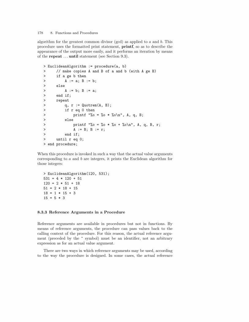
178 8. Functions and Procedures
algorithm for the greatest common divisor (gcd) as applied to a and b. Thisprocedure uses the formatted print statement, printf, so as to describe theappearance of the output more easily, and it performs an iteration by meansof the repeat . . .until statement (see Section 9.3).
> EuclideanAlgorithm := procedure(a, b)> // make copies A and B of a and b (with A ge B)> if a ge b then> A := a; B := b;> else> A := b; B := a;> end if;> repeat> q, r := Quotrem(A, B);> if r eq 0 then> printf "%o = %o * %o\n", A, q, B;> else> printf "%o = %o * %o + %o\n", A, q, B, r;> A := B; B := r;> end if;> until r eq 0;> end procedure;
When this procedure is invoked in such a way that the actual value argumentscorresponding to a and b are integers, it prints the Euclidean algorithm forthose integers:
> EuclideanAlgorithm(120, 531);531 = 4 * 120 + 51120 = 2 * 51 + 1851 = 2 * 18 + 1518 = 1 * 15 + 315 = 5 * 3
8.3.3 Reference Arguments in a Procedure
Reference arguments are available in procedures but not in functions. Bymeans of reference arguments, the procedure can pass values back to thecalling context of the procedure. For this reason, the actual reference argu-ment (preceded by the ~ symbol) must be an identifier, not an arbitraryexpression as for an actual value argument.
There are two ways in which reference arguments may be used, accordingto the way the procedure is designed. In some cases, the actual reference

8.3 User-Defined Procedures 179
argument is expected to have a value assigned to it before the procedure callbegins. This value will be used during the procedure call. By the time that theexecution has finished, it is possible that the corresponding formal referenceargument will have had a new value assigned to it; if so, the actual referenceargument will take on this value. Otherwise, the actual reference argumentwill retain the value it had before. In other cases, the actual reference ar-gument is merely an identifier name that does not have an assigned value.In this situation, the corresponding formal reference argument should not beused within the procedure body until it has had a value assigned to it. Atthe end of the procedure invocation, the final value of this formal referenceargument will be given to the actual reference argument.
As an example of the first case, consider ShiftR(˜Q) defined above. Inorder to be executed successfully, this procedure requires the actual referenceargument corresponding to Q to be an identifier that has a value (in partic-ular, a sequence) assigned to it. After the procedure invocation, the actualreference argument will in general have a new value.
As an example of the second case, in which the actual reference argumentdoes not have an initial value, consider a modification of EuclideanAlgorithm.Since the purpose of the Euclidean algorithm is to calculate the gcd, thisprocedure can easily be modified so that it returns the gcd via a referenceargument g:
> EuclideanAlgorithm := procedure(a, b, ~g)> // make copies A and B of a and b (with A ge B)> if a ge b then> A := a; B := b;> else> A := b; B := a;> end if;> repeat> q, r := Quotrem(A, B);> if r eq 0 then> printf "%o = %o * %o\n", A, q, B;> g := B; // store the gcd in g> else> printf "%o = %o * %o + %o\n", A, q, B, r;> A := B; B := r;> end if;> until r eq 0;> end procedure;
When the procedure EuclideanAlgorithm(a, b, ˜g) is called, the actual refer-ence argument must be an identifier (d, say). The gcd will be stored in d atthe end of the procedure invocation. Since the body of the procedure only

180 8. Functions and Procedures
makes an assignment to g, and does not attempt to use its value prior to thecall, it does not matter whether d has a value before the procedure call, butif it does, that value will be destroyed:
> d := "junk";> EuclideanAlgorithm(531, 120, ~d);531 = 4 * 120 + 51120 = 2 * 51 + 1851 = 2 * 18 + 1518 = 1 * 15 + 315 = 5 * 3> print d;3
In some other computer languages, it is advisable to use reference argu-ments rather than value arguments when passing values requiring a greatdeal of storage space. However, this technique is of no benefit in Magma,because the system uses reference counts to avoid making unnecessary copiesof value arguments.
8.3.4 Early Return from a Procedure Invocation
Since a procedure does not have return values in the sense of a function’sreturn values, it should not contain any statements of the form:
return expression, . . . , expression;
However, it may contain one or more lines of the form:
return;
The command return, when followed by a semicolon, instructs Magma tostop executing the procedure call immediately, without progressing throughthe rest of the procedure body down to end procedure.
For instance, EuclideanAlgorithm could be written in this way:
> EuclideanAlgorithm := procedure(a, b, ~g)> // make copies A and B of a and b (with A ge B)> if a ge b then> A := a; B := b;> else> A := b; B := a;> end if;

8.4 Local and Non-Local Identifiers 181
> repeat> q, r := Quotrem(A, B);> if r eq 0 then> printf "%o = %o * %o\n", A, q, B;> g := B; // store the gcd in g> return;> end if;> printf "%o = %o * %o + %o\n", A, q, B, r;> A := B; B := r;> until r eq 0;> end procedure;
Both versions are quite suitable in this case, but the return version has theadvantage that less indentation is required.
8.4 Local and Non-Local Identifiers
At this point it may seem that there is potential for great confusion be-tween identifiers of the same name residing inside and outside of a func-tion/procedure. What would happen, for instance, if when EuclideanAlgorithmwas called the identifiers a or A were already defined? Would it affect theoutcome of the procedure invocation, and would the values of these identifiersbe preserved? Magma has a simple principle known as the first textual userule to prevent problems like this. Any identifier which is a formal argument,or whose first appearance in the text of the function expression is for thepurpose of having a value assigned to it, is local to the function. This meansthat if there are identifiers with the same name existing outside the func-tion, they are not changed by a function call, and on the other hand, afterthe function call has finished execution, the function’s identifiers effectivelydisappear and those outside the function reappear.
The following lines illustrate this notion of local scope:
> a := 17; b := 62; c := 54;> multip := function(a, b)> c := a * b;> return c;> end function;> print multip(8, 9);72> print a, b, c;17 62 54

182 8. Functions and Procedures
Although the formal identifiers a and b are given the values 8 and 9 withinthe scope of the function, the values of the identifiers a and b outside thefunction do not change. Similarly, although the identifier c inside the functionis given the value 72, the value of the identifier c outside the function does notchange. Therefore anyone can use the function multip by knowing merely thatit returns the product of its two arguments. As is appropriate, the internalworkings of the function are irrelevant to its use.
Identifiers in functions are not always local. If the first time that an iden-tifier appears is when it is referred to in an expression rather than when it isassigned, then Magma looks for its value outside the function. For example:
> sarah := 42;> silly := function(blanche)> diana := sarah * (3 - blanche);> return diana^2 + sarah;> end function;> print silly(6);15918
The first textual use of sarah in the function body of silly is in the expressionsarah*(3 − blanche). Therefore sarah is a non-local identifier, and Magmawill use the value which sarah has been assigned outside the function. Theresult is that silly is defined exactly as if it had been:
> silly := function(blanche)> diana := 42 * (3 - blanche);> return diana^2 + 42;> end function;
Note that if the value of sarah is now changed, the function silly will remainas it was before, although its definition included the use of sarah. Only thecurrent values of identifiers are relevant when a function is being defined:
> sarah := 100000;> print silly(6);15918
It is generally unwise to use non-local identifiers within a function. Thedanger is that the function could be defined at a time when its non-local iden-tifiers are set incorrectly; this can easily happen, especially when a function isin the development stage. A non-local identifier should only be used in a func-tion definition when it can be guaranteed that its value will be as expected.For instance, the identifier might have been given its value only a short whilebefore, or it might be an identifier that the user is in the habit of using forspecial purposes, such as Z for IntegerRing() or R for RealField().

8.5 Functions and Procedures as First-Class Objects 183
Non-local identifiers cannot be reassigned within a function body. In this,they resemble loop identifiers in for-statements. Magma sees both of these asmembers of the value class of identifiers, rather than as ‘variable identifiers’in the sense of objects that can be varied by the user.
It should be noted that formal value arguments are local identifiers withina function body, and may be re-assigned. For example:
> blanche := "bob";> silly := function(blanche)> blanche := 3 - blanche;> diana := 42 * blanche;> return diana^2 + 42;> end function;> print silly(6), blanche;15918 bob
8.5 Functions and Procedures as First-Class Objects
Functions and procedures are first-class objects. They can be assigned toidentifiers, as shown throughout this chapter, but they can also be passedinto functions and procedures, or obtained as return values of functions. Forinstance, the following function trapezoid calculates an approximation to theintegral of a single-argument real function f from a to b, using one applicationof the trapezoidal rule:
> trapezoid := func< f, a, b | (b-a)/2 * (f(a) + f(b)) >;> print trapezoid(Sin, 2, 5);-0.07444027175618516025> myfunc := func< x | x^3 - Log(x) >;> print trapezoid(myfunc, 1, 10);4494.1383670815267944
The example shows trapezoid being applied to the system intrinsic functionSin and then to the user-defined function myfunc.
8.6 Recursion
A function or procedure is allowed to invoke itself within its own definition.This phenomenon is known as recursion. Recursion is used when it is difficultto solve a problem directly, but it is possible to reduce it to a slightly smaller

184 8. Functions and Procedures
problem of the same kind. One then reduces the slightly simpler problem,and so on until arriving at a problem which is so simple that it can be solveddirectly.
For example, suppose Q is a non-empty sequence of integers and itis necessary to find the smallest term, m. The system intrinsic functionMinimum(Q) performs this task exactly, but it is worth exploring how towrite a recursive function for a situation such as this. The function will usea less powerful version of the system intrinsic, the Minimum(a, b) function,which returns the smaller of the two numbers a and b.
A recursive function smallest(Q) may be written for this task using eitherthe constructor form or the statement form of a function expression. Thestatement form will be used here, so that the parts of the function can bedisplayed more easily.
The function should begin with a heading that gives Q as the formalidentifier:
> smallest := function(Q)
Next, it is necessary to consider when the problem can be solved directly. Inthis example, finding the minimum term of Q is trivial when Q has only oneterm, so the body of the function can begin as follows:
> if #Q eq 1 then> return Q[1];
The function body must continue with instructions in the case that Qhas more than one term. The insight to be had here is that to find theminimum of a sequence of size n, one can take the last term from the sequence,find the minimum of the remaining sequence of size (n − 1), and comparethis minimum with the removed term by means of Minimum(a, b). Thisobservation is useful because it reduces the problem to that of finding theminimum of a sequence which has one term fewer. Finding the minimum ofthis smaller sequence can be done by first finding the minimum of a sequencewhich is smaller again, and so on until the sequence is reduced to size 1, acase which has already been covered by the if–then section. The else-clausebelow encodes this insight:
> else> finalterm := Q[#Q];> prunedmin := $$(Prune(Q));> return Minimum(finalterm, prunedmin);> end if;

8.7 The forward-declaration 185
The $$ sign in the above stands for the function currently being defined, inthis case smallest . It is not possible to use the name smallest at this point,because within the statement body of the function expression the identifiersmallest is undefined (unless it happens by coincidence to have a value as-signed to it already). Only after Magma has processed the whole functionexpression can it assign the function to smallest . (See p. 188 for an exceptionto this.)
The full function smallest is:
> smallest := function(Q)> if #Q eq 1 then> return Q[1];> else> finalterm := Q[#Q];> prunedmin := $$(Prune(Q));> return Minimum(finalterm, prunedmin);> end if;> end function;
For example:
> print smallest([5, 2, 4, 4, 65, 31]);2
The $$ symbol is also recognized within the func-constructor. For ex-ample, the function smallest(Q) may be defined using func, as remarkedpreviously:
> smallest := func< Q |> #Q eq 1 select Q[1]> else Minimum(Q[#Q], $$(Prune(Q))) >;
Recursive functions and procedures are characterized by this elegance,but they must be written with care. The user must ensure that the recursionwill eventually terminate, irrespective of the values of the actual arguments.
8.7 The forward-declaration
Suppose that a function/procedure f is about to be defined which invokesa function/procedure according to the identifier g. If g has not yet beenassigned a function/procedure, Magma will give an error message when itencounters the use of g within the definition of f . To prevent this error, it ispossible to type

186 8. Functions and Procedures
> forward g;
before the definition of f begins. This forward-declaration is an indicationto Magma that g will be assigned a function/procedure later. Any numberof functions/procedures may now be defined with expressions involving invo-cations of g. However, the system expects that before the invocation of f (orany other function/procedure whose definition involves g), g will have beenassigned.
The forward-declaration must occur on the main level, not within a func-tion/procedure definition. If several functions/procedures are to have thesedeclarations, they may either have separate forward-declarations or be givenin a comma-separated list following the word forward.
There are two major applications for the forward-declaration. The firstusage is a matter of convenience, but the second one is a matter of necessity.Firstly, some programmers like to place their principal programs before thesmaller programs that support them (in a file, for instance). If they wish to beable to order their functions/procedures in this way, they must precede thedefinition of the principal functions/procedures with forward-declarationsfor the other functions/procedures. Here is an example in miniature; it calcu-lates the number of steps required in the 3n+1 problem to reduce a positiveinteger n to 1, following the rule that if n is odd, then n 7→ 3n + 1, and if nis even, n 7→ n
2 . The principal function is Nsteps(n), and it is supported bythe functions oe, odd , and even. Note also that Nsteps is recursive.
> forward oe, odd, even;> Nsteps := func< n | n le 1 select 0 else 1 + $$(oe(n)) >;> oe := func< n | IsOdd(n) select odd(n) else even(n) >;> odd := func< n | 3*n + 1 >;> even := func< n | n div 2 >;>> print Nsteps(34), Nsteps(871);13 178
The second usage for the forward-declaration is in cases of mutual re-cursion. If f and g are mutually recursive functions/procedures, that is, ifthey invoke one another, the user must make a forward-declaration of g,then define f , then define g [or vice versa]. The functions/procedures f andg should be designed so that the mutual recursion terminates eventually.
For example, the following function isPrime(n) is a [rather poor] imitationof the system intrinsic IsPrime(n). For odd n > 3 it first checks for a few(3) random values of an integer a in the range 2 to n − 2 that an−1 ≡ 1(mod n). If this is false, then n cannot be prime; if it is true, then a primalityprover strongTest(primdiv , n) is applied, where primdiv is the sequence of

8.8 Function Assignment and Procedure Assignment 187
prime divisors of n− 1. It uses the theorem that n is prime if there exists aninteger x in the range 2 to n− 1 such that xn−1 ≡ 1 (mod n) and x
n−1p 6≡ 1
(mod n) for all prime divisors p of n−1. A third function, primeDivisors(n),is needed to find primdiv . This function is both self-recursive and mutuallyrecursive with isPrime. In the ordering of the functions below, there is aforward-declaration of primeDivisors, followed by the definition of isPrime,followed by the definition of primeDivisors:
> strongTest := func< primdiv, n |> exists x : x in [2..n-1] |> Modexp(x, n-1, n) eq 1 and> forall p : p in primdiv |> Modexp(x, (n-1) div p, n) ne 1 >;> forward primeDivisors;> isPrime := func< n |> n in 2, 3 or IsOdd(n) and> forall i : i in [1..3] |> Modexp(Random(2, n-2), n-1, n) eq 1 > and strongTest(primeDivisors(n-1), n) >;> primeDivisors := func< n |> isPrime(n) select n else> ($$(d) join $$(n div d) where d is> rep d : d in [2..Isqrt(n)] | n mod d eq 0 ) >;>> print isPrime(137821), isPrime(12853);false true
8.8 Function Assignment and Procedure Assignment
Functions and procedures both have variants of the statement form. Insteadof beginning a definition with the line
R := function(formal arguments)
or
R := procedure(formal arguments)
the user can start with
function R(formal arguments)
or

188 8. Functions and Procedures
procedure R(formal arguments)
and then continue as explained previously. These construtions are the func-tion assignment statement and procedure assignment statement. Some usersmay find this syntax more convenient, particularly if they are accustomedto it from other programming languages. The effect in Magma is the same,except for a slight difference in recursive routines. If this form is used, thenwithin the function or procedure definition the routine may be called by itsname R instead of by the pseudo-name $$.
In more detail, when Magma encounters a function assignment statement(similarly for a procedure), it internally transforms it into the assignment ofthe value of a function expression to the given function name. Before assigningthe expression’s value, it rewrites any instances of the function name withinthe function expression as $$, so that a recursive function or procedure’s ownname may be used during its definition by this method.
For example, the function smallest defined on p. 185 may be redefinedusing this technique as follows:
> function smallest(Q)> if #Q eq 1 then> return Q[1];> else> finalterm := Q[#Q];> prunedmin := smallest(Prune(Q));> return Minimum(finalterm, prunedmin);> end if;> end function;
8.9 Error Messages
Users designing a function or procedure must take care that it can cater forall kinds of input in the actual arguments. Otherwise the behaviour will beunpredictable. The routine may stop, with a confusing or misleading errormessage, or (even worse) it may complete its execution but give an undesiredresult.
Magma has an error-statement which can be used to assist in this task.The form of the error-statement is:
error expression, . . . , expression;

8.9 Error Messages 189
If Magma encounters an error-statement while executing a procedure callor function call, it prints the values of the expressions, as it would for aprint-statement, and also breaks out of the call.
A related statement is the error if statement, with the form:
error if condition, expression, . . . , expression;
If Magma encounters this statement while executing a procedure call orfunction call, it evaluates the Boolean condition immediately after error if.If the condition is false, Magma ignores the rest of the statement. However,if it is true, then Magma acts as for a plain error-statement, by printingthe values of the expressions, and breaking out of the call.
If a function invocation is being executed and Magma encounters eitheran error-statement or an error if with a true condition, then the functioncall does not return a value.
As an example of error-handling, consider SeparatingLine(c, n) definedon p. 177. Some improvements can be made to this procedure by testing forlikely errors. As it stands at present, if the user confuses the order of thearguments and types
> SeparatingLine(10, "!");
>> print c^n;^
Runtime error in ’^’: Bad argument types
then the error message is very unhelpful for a user who has never seen theprocedure definition body. It would be better to check the categories of thearguments as soon as execution of the procedure call commences. This alsoapplies to the following call, where the ^ operator happens to work but doesnot perform the intended string concatenation:
> S6<a, b> := Sym(6);> SeparatingLine(b, a^3);(4, 5)
Another possible error that should be detected is the entry of an unsuitableinteger for n. The procedure should check that n is non-negative, and lessthan some reasonable line-length bound such as 80.
With these ideas in mind, the revised procedure can be either of these(demonstrating both kinds of error statements):
> SepLine := procedure(c, n)

190 8. Functions and Procedures
> if Type(c) ne MonStgElt or Type(n) ne RngIntElt then> error "Error in ’SepLine’: Bad argument types";> elif n notin [0..80] then> error "Error in ’SepLine’: Argument 2 (", n,> ") not in range [0..80]";> else> print c^n;> end if;> end procedure;
> SepLine := procedure(c, n)> error if Type(c) ne MonStgElt or Type(n) ne RngIntElt,> "Error in ’SepLine’: Bad argument types";> error if n notin [0..80],> "Error in ’SepLine’: Argument 2 (", n,> ") not in range [0..80]";> print c^n;> end procedure;
These two procedures have the same effect, but error if is preferable sincethis kind of error situation can be detected with a simple test of a condition.
SepLine (either version) works in the same way as SeparatingLine if theinput is legal, but otherwise it produces error messages such as the following:
> SepLine(10, "!");Error in ’SepLine’: Bad argument types> SepLine("$", 2000);Error in ’SepLine’: Argument 2 ( 2000 ) not in range [0..80]
Further error checks might also be desirable, such as ensuring that c has onlyone character.
Not all runtime errors can be found so easily. The ones shown abovecould be detected at the beginning of the call, but sometimes errors can onlybe found after several of the computations in the routine have taken place.Functions and procedures should be robust enough to deal intelligently witherrors such as these as well.
If a function or procedure is sufficiently useful to be converted into auser intrinsic, then certain aspects of error-checking become easier. Category-checking of arguments becomes automatic, and there are additional state-ments for error-handling. See Section 10.8.

8.10 Parameters 191
8.10 Parameters
Many of Magma’s system intrinsics that encode the more complicated algo-rithms have parameters available. User-defined functions and procedures anduser intrinsics may also have parameters. Parameters are like optional argu-ments, whose purpose is to control some aspect of the algorithm’s execution.This kind of control could be maintained with ordinary value identifiers, butthe advantage of a parameter is that it need only be referred to in a functionor procedure call if the user wishes its value to be other than the standard ordefault value. For every parameter in an algorithm, the algorithm designermust decide what the most often desired value of the parameter will be, andspecify it as the default value. If the function or procedure call includes anassignment to the parameter, the given value will be used for it; otherwise,the default value will be used.
Parameter names follow the rules of identifier names. They are specific tothe function or procedure, and have local scope. Thus if a function/procedurehas a parameter with the same name as a current identifier, there will beno confusion between their values; nor will there be confusion with anotherfunction/procedure with the same parameter name.
For each system intrinsic, the online help system includes the name anddefault value of every parameter, a list or description of the parameter’spossible values, and a description of how the values of the parameters affectthe behaviour of the function or procedure.
8.10.1 Parameters in Function or Procedure Calls
The syntax for a call to a function or procedure R that has parameters is:
R(arguments : parameter := expr, ..., parameter := expr)
Observe that all the actual value and reference arguments are given, thena colon, then a comma-separated list of the parameters and their values. Itis only necessary to list those parameters which are being given non-defaultvalues (though it is permissible to list them even if the values are default). Theorder in which the parameters and their values are listed is not important.
For instance, the system intrinsic function IsSubsequence(Q,T ) returnstrue if Q is a subsequence of T , else false. However, since there is someflexibility in the definition of a subsequence, the user may specify what kindof subsequence is intended using the parameter Kind. The default valueof Kind is "Consecutive", meaning that the elements of Q must occurconsecutively in T . Therefore the function IsSubsequence may be used

192 8. Functions and Procedures
without reference to the parameter Kind when a consecutive subsequence isintended:
> F3<a, b, c> := FreeGroup(3);> T := [ a*b, b^2, a*c^-5, c*a*b, Id(F3), b^-2 ];> print IsSubsequence([ b^2, a*c^-5 ], T);true> Q := [ a*b, a*c^-5 ];> print IsSubsequence(Q, T);false
The other possible values for the parameter Kind are "Sequential", mean-ing that the elements of Q must occur in T in the same indexing order, and"Setwise", meaning that the elements of Q must occur in T but that theindexing order is irrelevant. If one of these parameter values is required, theactual arguments in the function call must be followed by a colon, then theparameter name, an assignment symbol (:=), and the value of the parameter.For instance:
> print IsSubsequence(Q, T : Kind := "Sequential");true
As an example of a function with several parameters, consider Factor(n),which attempts to find a proper factor q of n. (See Section ?? for a fullexplanation of this system intrinsic.) Factor has several parameters, the mostimportant being Al, which specifies the particular factorization method oralgorithm to be used within the overall algorithm. One of the possible valuesof Al is "Division", the trial division method:
> print Factor(143 : Al := "Division");11 13
If Al is assigned this value, there are two other parameters used by Factor aswell, Lower and Upper, giving the lower and upper bounds for the search fordivisors. (Factor has additional parameters, suitable for different choices ofAl, but their values will be ignored in this case.) The default value of Loweris 2, and the default value of Upper is min(Lower+1000,
√n). These default
bounds are chosen so that every moderately small factor will be found andthe execution time will not be large. However, for a large n the function mayfail to find a proper factor q; this is indicated by returning 1 and n instead ofq and n
q . If this occurs, the user may wish to increase Upper. For instance:
> n := NextPrime(1000) * NextPrime(1020);> print Factor(n : Al := "Division");1 1030189

8.10 Parameters 193
> // increase Upper> print Factor(n : Al := "Division", Upper := 1100);1009 1021
8.10.2 Parameters in Function or Procedure Definitions
All the methods of construction for user-defined functions and proceduresmay be adapted to cater for parameters. The syntax is similar to that usedin the function/procedure call: following the formal arguments comes a colon,and then a comma-separated list of parameter assignments. The values as-signed to the parameters are the default values.
A simple example of parameters in a user-defined procedure may be givenby a modification of the earliest version of SeparatingLine (p. 177). Thefunction below prints k lines of output, consisting of n copies of the characterc. The identifier k is a value argument, but c and n are parameters, withdefault values "*" and 60:
> SeparatingBlock := procedure(k : c := "*", n := 60)> for i in [1..k] do> print c^n;> end for;> end procedure;
> SeparatingBlock(3);************************************************************************************************************************************************************************************> SeparatingBlock(2 : n := 13, c := "&");&&&&&&&&&&&&&&&&&&&&&&&&&&> SeparatingBlock(4 : c := "#");################################################################################################################################################################################################################################################
As an example of parameters in a func-constructor, consider the func-tion trapezoid(f, a, b) given on p. 183, which returns an approximation to∫ b
af(x) dx using one application of the trapezoidal rule. It may be easily be
extended to use n applications of the rule, where n is a positive integer. Thereare two ways to program this modification. Either the function can be createdwith another value argument n, or it can be created with n as a parameter.

194 8. Functions and Procedures
Both options are shown below; for the parameter version, the default valueof n is 10:
To perform this example online, type load "I96c8e2";
trapezoidN1 := func< f, a, b, n |h/2 * ( f(a) + f(b) +
2 * &+[ RealField() | f(a + k*h): k in [1..(n-1)]] )where h is (b - a) / n >;
trapezoidN2 := func< f, a, b : n := 10 |h/2 * ( f(a) + f(b) +
2 * &+[ RealField() | f(a + k*h): k in [1..(n-1)]] )where h is (b - a) / n >;
> print trapezoidN1(Sin, 2, 5, 10);-0.694552564585352346417694621390712060130> print trapezoidN1(Sin, 2, 5, 3);-0.640495911166789416020461561894692590284
> print trapezoidN2(Sin, 2, 5);-0.694552564585352346417694621390712060130> print trapezoidN2(Sin, 2, 5 : n := 3);-0.640495911166789416020461561894692590284
The decision as to whether n should be a parameter or a value argumentdepends on whether a default value can be found for n that would be thedesired value most of the time.
Now, another common method of quadrature (approximate integration)is Simpson’s rule. The function quadrature below provides access to boththe trapezoid rule and Simpson’s rule. It has two parameters: Al , a stringwhich takes the value "Trapezoid" (the default) or "Simpson"; and n, apositive integer (default 10) giving the number of applications of the rule. Thefunction includes some tests to see that the values given to the parametersin the function call are legal; for brevity, the legality of the actual argumentsis assumed.
To perform this example online, type load "I96c8e3";
> quadrature := function( f, a, b : Al := "Trapezoid", n := 10)> // Check that parameter values are legal> error if Category(n) ne RngIntElt or n lt 1,> "Error: n not a positive integer";> error if Category(Al) ne MonStgElt

8.11 The assert-statement 195
> or Al notin "Trapezoid", "Simpson",> "Error: Al must be \"Trapezoid\" or \"Simpson\"";>> R := RealField();> h := (b - a) / n;> if Al eq "Trapezoid" then> return h/2 * ( f(a) + f(b) +> 2* &+[ R | f(a + k*h): k in [1..(n-1)]] );> else // "Simpson" method> return h/3 * ( f(a) + f(b) +> 4 * &+[ R | f(a + k*h): k in [1..(n-1) by 2]] +> 2 * &+[ R | f(a + k*h): k in [2..(n-2) by 2]] );> end if;> end function;
This function may be used as follows:
> print quadrature(Sin, 2, 5);-0.694552564585352346417694621390712060130> print quadrature(Sin, 2, 5 : Al := "misprint");Error: Al must be "Trapezoid" or "Simpson"> print quadrature(Sin, 2, 5 : Al := "Simpson");-0.699840854042387310477518928061320632823> print quadrature(Sin, 2, 5 : n := 100);-0.699756535546415853278023992585548468613> print quadrature(Sin, 2, 5 : Al := "Simpson", n := 100);-0.699809025159846690320174742187892306263> // compare with use of exact integral> print -Cos(5) + Cos(2);-0.69980902201036865146420740109
Note that Magma has an intrinsic Integral(f, a, b) which performs a similartask. However, the first argument in Integral is a map, not a function.
8.11 The assert-statement
The assert-statement has the following syntax:
assert condition;
where the condition is an expression that evaluates to a Boolean. The effectof this statement depends on the value of the condition when the statementis executed: if it is true, Magma does nothing; if it is false, Magma stopsexecution and gives an error message, stating that the assertion failed.

196 8. Functions and Procedures
This statement is provided as a preventative against errors in program-ming. If it is included in the statement body of a function or proceduredefinition, then the assertion made in the condition will be checked each timeit is encountered during an invocation of that function/procedure. The asser-tion should express a fact that must be true at that point in the statementbody.
For example, in the EuclideanAlgorithm procedure discussed in earliersections of this chapter, the value of gcd(a, b) is calculated by means of theEuclidean algorithm and assigned to g. It would be wise to check that theimplementation of the algorithm is correct by calculating the greatest com-mon divisor another way, with the kernel intrinsic function GCD(a, b), andasserting that this value equals g:
> EuclideanAlgorithm := procedure(a, b, ~g)> // make copies A and B of a and b (with A ge B)> if a ge b then> A := a; B := b;> else> A := b; B := a;> end if;> repeat> q, r := Quotrem(A, B);> if r eq 0 then> printf "%o = %o * %o\n", A, q, B;> g := B; // store the gcd in g> assert g eq GCD(a, b);> return;> end if;> printf "%o = %o * %o + %o\n", A, q, B, r;> A := B; B := r;> until r eq 0;> end procedure;
Since the implementation of the algorithm is indeed correct, the assert-statement will have no effect on invocations of the procedure from the caller’spoint of view.
It is possible for the user to control whether assertions are checked, accord-ing to the value of GetAssertions(). By default, this function returns true(i.e., check the assertions). However, the procedure call SetAssertions(b),where b is a Boolean, may be used to change this. If b is set to false, thenMagma will ignore assert-statements entirely, thus reducing the executiontime slightly.

9. Iterative Statements
Iteration or looping is the repeated performance of a task that is syntacticallyconstant but for which the data may change. The terms iteration or loop mayalso be applied to instances of the task’s performance. The classic methodof specifying iteration in computer languages is by means of iterative state-ments. These are compound statements, since they surround other statementsproviding the description of the task which is to be performed repeatedly. Asthis chapter explains, Magma has three forms of iterative statements: thewhile-statement, the repeat-statement, and the for-statement.
It should be noted at the outset that iterative statements are not as cru-cial for programming in the Magma language as they are in many othercomputer languages. Magma’s set and sequence constructors allow many it-eration processes to be expressed statically, as a description of the outcomerather than as an explicit iteration using an iterative statement. By the na-ture of elementary examples, many of the iteration tasks in this chapter arealso programmable using set/sequence constructors. Nonetheless, there areapplications for which iterative statements remain the best or only choice ofprogramming tool in the Magma language.
9.1 Methods of Iteration
In most cases of iterative processes, the programmer intends the whole iter-ation to stop at the end of one of the loops. There are two ways of statingwhen this is to happen: either the iteration is over a predetermined finitedomain D, and continues until some identifier has assumed each value of Dexactly once in successive loops; or, less predictably, a Boolean expressionis evaluated at the beginning or end of each loop, and the iteration processconcludes when the value of this expression changes. Occasionally, it is moreconvenient for the iteration to conclude in the midst of one of the loops; thismay be achieved by means of an interrupt that follows upon the change invalue of some intermediate condition.

198 9. Iterative Statements
Magma’s iterative statements provide for all these circumstances. In oneof them, the for-statement, the iteration is over a domain, according to thefirst kind of termination condition. In the others, the while-statement andrepeat-statement, termination is dependent on the value of a Boolean ex-pression that is evaluated respectively at the beginning and end of each loop.Magma also provides statements for interrupting the usual course of theiterative statement: the break-statement for immediate termination of thewhole iterative statement, and the continue-statement for termination ofthe current loop of the iteration.
Magma’s set and sequence constructors, and related syntactic constructs,allow many kinds of iteration to be performed without the need for iterativestatements. For example, the following set constructor creates the set of in-tegers of the form p3, where p is a prime in the range 1 ≤ p ≤ 20:
> PrimesCubed := p^3 : p in [1..20] | IsPrime(p) ;> print PrimesCubed; 8, 27, 125, 343, 1331, 2197, 4913, 6859
Although this set is described statically, iteration takes place internally.Magma must iterate over the domain sequence [1..20], and for each ele-ment p of the domain it must test its primality and then, for the primes only,include the value of p3 in a set. In many programming languages, this taskwould have to be expressed as an explicit iteration. The Magma version ofsuch an iteration would use a for-statement, because it is an iteration over apredetermined domain:
> PrimesCubed := ;> for p in [1..20] do> if IsPrime(p) then> Include(~PrimesCubed, p^3);> end if;> end for;> print PrimesCubed; 8, 27, 125, 343, 1331, 2197, 4913, 6859
Note that this method of constructing the set is more verbose, and is alsomore difficult to write and understand. In general, Magma style favoursconstructors over iterative statements when the task to be performed is rela-tively simple. However, if the task contains many auxiliary identifiers, manyoperations, or many print-statements, then an iterative statement should bechosen, since a constructor will be impossible or cumbersome.
It should be remembered that in most cases the choice of a method ofiteration for an algorithm affects the time taken to develop the code muchmore than the execution time. Convenience for the programmer and legibility

9.2 The while-statement 199
of the program are the most important factors in the decision, except whenthe computations are going to consume a significant amount of CPU time.
9.2 The while-statement
The syntax of the while-statement is
while Boolean expression dostatements
end while;
where there must be at least one statement between do and end while; thesestatements constitute the task to be iterated. The termination condition forthe iteration process is given by the Boolean expression following while. Thisexpression is evaluated at the beginning of each loop, including the first loop.If it is true, then the loop is executed; otherwise, the execution of the wholewhile-statement finishes. Note that if the value of the Boolean expressionis already false before the looping has started, then the statement body isnever executed.
For example, consider the problem of calculating the factorial of n.(Magma has an intrinsic function Factorial(n) that should be used in prac-tice to find this value.) Initially, the value of n will be fixed at 20. Thefollowing lines of code, incorporating a while-statement, cause the value of20! to be stored in the identifier answer :
> n := 20;> c := n;> answer := 1;> while c gt 0 do> answer *:= c;> c -:= 1;> end while;
When this program is typed into Magma, the computer will probably providea special prompt during the time that the statement body of the while-statement is being entered, as a reminder that end while has not yet beentyped:
> n := 20;> c := n;> answer := 1;> while c gt 0 do

200 9. Iterative Statements
while> answer *:= c;while> c -:= 1;while> end while;
The special prompt will usually be omitted in the examples in this chapter,for the sake of clarity.
When an iterative statement is typed into Magma, if the system detectsan error before the end of the whole statement has been reached, then the partof the statement already typed is lost. It may be recovered with Magma’shistory-editing facilities, but for longer iterative statements it is helpful todevelop them in an external file and load the file into Magma. See Section14.2.
After the iterative statement has terminated, the number 20! will be storedin answer . It may be compared with the value returned by Factorial(n):
> print answer;2432902008176640000> print Factorial(n);2432902008176640000
The workings of the code above will now be explained in detail. The firststatements this program executes are the assignments to n, c and answer . Thereason for creating c as a copy of n is that the algorithm requires the value ofn to be gradually decremented, but it may be undesirable to lose the originalvalue of n. Next comes the while-statement. The first step in executing awhile-statement is to evaluate the condition given between while and do.Since c is indeed greater than 0, Magma starts executing the statementsbetween do and end while. On this first pass through the loop, answer is 1and c is 20, so the line
> answer *:= c;
multiplies answer by c, making answer become 20. The other statement inthe loop reduces c by 1. Magma now evaluates the while-condition again,and finds that it is still true, since 19 > 0. Thus the loop statements areexecuted again. This time answer becomes 20× 19 and c becomes 18. Afterseveral more iterations, execution of the loop reaches the stage when the valueof c is 1. This time answer becomes (20×19×· · ·×2)×1 = 20! and c becomes0. Magma evaluates the while-condition yet again, but it is no longer true,because 0 gt 0 is false. Now execution of the program falls through to theline following end while, and answer has its final value of 20!.
From the trace-through of the iteration, some ways to improve this algo-rithm should be readily apparent. The last pass through the loop serves no

9.2 The while-statement 201
purpose, because answer already equals 20! and is merely being multipliedby 1. Moreover, the very first pass through the loop could be eliminated bya change in the initial assignments to c and answer . A version incorporatingthese refinements appears below:
> c := n - 1;> answer := n;> while c gt 1 do> answer *:= c;> c -:= 1;> end while;
It is now appropriate to generalize this code for all integers n ≥ 0. Thecode will be enclosed in a function, for ease of use:
To perform this example online, type load "I96c9e1";
> factl := function(n)> error if n lt 0,> "Error in ’factl’: Argument should be >= 0";> if n lt 2 then> return 1;> end if;> c := n - 1;> answer := n;> while c gt 1 do> answer *:= c;> c -:= 1;> end while;> return answer;> end function;
To obtain the value of n! for various n, the function factl may be called asfollows:
> print factl(5);120> print factl(-241);Error in ’factl’: Argument should be >= 0> print factl(0);1> print factl(17);355687428096000
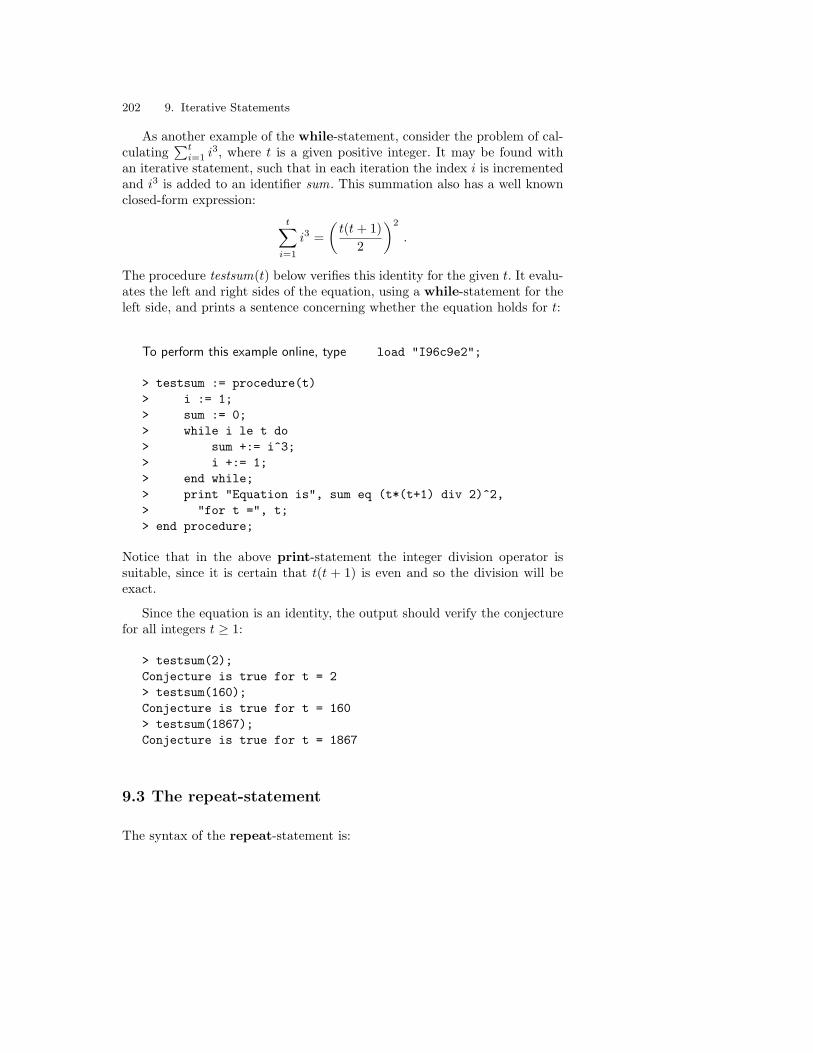
202 9. Iterative Statements
As another example of the while-statement, consider the problem of cal-culating
∑ti=1 i3, where t is a given positive integer. It may be found with
an iterative statement, such that in each iteration the index i is incrementedand i3 is added to an identifier sum. This summation also has a well knownclosed-form expression:
t∑
i=1
i3 =(
t(t + 1)2
)2
.
The procedure testsum(t) below verifies this identity for the given t. It evalu-ates the left and right sides of the equation, using a while-statement for theleft side, and prints a sentence concerning whether the equation holds for t:
To perform this example online, type load "I96c9e2";
> testsum := procedure(t)> i := 1;> sum := 0;> while i le t do> sum +:= i^3;> i +:= 1;> end while;> print "Equation is", sum eq (t*(t+1) div 2)^2,> "for t =", t;> end procedure;
Notice that in the above print-statement the integer division operator issuitable, since it is certain that t(t + 1) is even and so the division will beexact.
Since the equation is an identity, the output should verify the conjecturefor all integers t ≥ 1:
> testsum(2);Conjecture is true for t = 2> testsum(160);Conjecture is true for t = 160> testsum(1867);Conjecture is true for t = 1867
9.3 The repeat-statement
The syntax of the repeat-statement is:

9.3 The repeat-statement 203
repeatstatements
until Boolean expression;
It is similar to the while-statement, except that the termination conditionis tested at the end, not the beginning, of each loop. The iteration continuesuntil the Boolean expression evaluates to true. Therefore the statement bodyis always executed at least once in this kind of iterative statement.
An example of a repeat-statement that tests a conjecture will now begiven. In 1640, Pierre Fermat made the conjecture that 22n
+ 1 is a primefor all positive integers n. Numbers of this form are now known as Fermatnumbers. The program below investigates the primality of the first six Fermatnumbers, and stops if it encounters one that is not prime. It uses the intrinsicfunction IsPrime, thus making the task much easier than in Fermat’s day.A repeat-statement is a slightly better choice than a while-statement forthis situation because at least one pass through the loop must be made, forthe calculation and testing of the first Fermat number. Because it is notclear whether the iterative process might finish when all six numbers havebeen tested or when a composite Fermat number has been found, the until-condition must consist of two conditions, joined by or. The program to testFermat’s conjecture follows:
> n := 1;> repeat> composite := not IsPrime(2^2^n + 1);> if composite then> print "Conjecture is false, since";> print "(2^2^", n, "+ 1) is composite.";> else> n +:= 1;> end if;> until composite or n eq 7;Conjecture is false, since(2^2^ 5 + 1) is composite.
The output shows what was discovered by Euler almost a hundred years afterFermat’s conjecture: the fifth Fermat number is not a prime. Fermat num-bers are still of interest to mathematicians, however; computational numbertheorists continue to investigate primality and factorization issues connectedwith them.
As another example of the repeat-statement, cconsider the calculation ofFibonacci numbers according to the recurrence relation Fn = Fn−1+Fn−2, forn > 2, with F1 = 1, F2 = 1. Two functions, employing different algorithms,will be discussed for constructing the sequence of all the Fibonacci numbers

204 9. Iterative Statements
less than some given large limit L. (Note that Magma’s intrinsic functionFibonacci(n) returns individual Fibonacci numbers Fn.)
The first algorithm involves three identifiers, called old , middle and new .At each stage, the two Fibonacci numbers most recently stored in the se-quence are in old and middle, and their sum is assigned to new and put onthe end of the sequence. Then middle is shifted to old , and new to middle, sothat the process can be repeated. This algorithm can be encoded as follows:
To perform this example online, type load "I96c9e3";
> fiboA := function(L)> middle := 1;> new := 1;> Q := [1];> repeat> Append(~Q, new);> old := middle;> middle := new;> new := old + middle;> until new ge L;> return Q;> end function;
The second approach to the Fibonacci problem comes from realizing thatthe numbers only have to be held in their identifiers to calculate the next twoterms of the sequence. Hence it might be more efficient to do calculations inpairs, rather than shifting the numbers from one identifier to another. Thisidea is incorporated in the following function:
To perform this example online, type load "I96c9e4";
> fiboB := function(L)> f := 1;> g := 1;> Q := [1];> repeat> Append(~Q, g);> f +:= g;> Append(~Q, f);> g +:= f;> until g ge L;> if f ge L then> Prune(~Q);

9.4 The for-statement 205
> end if;> return Q;> end function;
Notice that the final if-statement checks to see whether the final addition tothe sequence was greater than L. It is not possible to avoid the risk of over-shooting the limit L in this algorithm, without making the code inefficient.The size of g is always checked by the until condition before it is put on theend of the sequence, but if f were also checked before being appended to thesequence there would be another statement in the loop body, to be executedon every iteration.
Magma’s time command may be used to compare these algorithms forspeed. When time is placed at the beginning of a statement, the statement isexecuted as usual, but the number of seconds of CPU time taken to executethe statement is also printed. The following example demonstrates how totime both functions, with a limit L of 109000:
> L := 10 ^ 9000;> time fibonacciA := fiboA(L);Time: 2.919> time fibonacciB := fiboB(L);Time: 2.669> print fibonacciA eq fibonacciB;true> print #fibonacciA;43066
From the time comparison, fiboB is slightly faster than fiboA for this valueof L.
9.4 The for-statement
The general structure of the for-statement is
for identifier in domain dostatements
end for;
The loop identifier, following the word for, takes the elements in the domainas its successive values, and for each value of the identifier, the statements areexecuted. Typically they would include some reference to the loop identifier.The domain of the loop identifier should be an expression that evaluates

206 9. Iterative Statements
to some iterable structure, that is, an iterable aggregate structure or a finitemagma whose elements Magma is able to list. This domain is calculated whenthe execution of the for-statement begins, and cannot be changed during theiteration.
For example, consider the residue class ring ZZ18 of integers modulo 18.Some of the elements n of this ring are squares, in the sense that there existsan element m of the ring such that m2 = n. One way to identify these squaresis to test each element of the ring in turn, using the function IsSquare(n).The for-statement below does this, using the residue class ring as its domain:
> for n in ResidueClassRing(18) do> if IsSquare(n) then> print n;> end if;> end for;01479101316
To execute the for-statement above, Magma initially assigns to n the firstelement of ZZ18 delivered to it by the iteration mechanism for this ring. Thenit performs everything between the do and the end for, using this value ofn. Next, n is assigned the second element of the ring and the body of thefor-loop is executed again, with the new value of n. The process continuesuntil the loop body has been executed for each element of the domain.
As another example, let G be a permutation group. The elements of G oforder k may be collected into a set by means of a for-statement. The functionbelow returns this set for a given group G and integer k:
To perform this example online, type load "I96c9e5";
> order_elts := function(G, k)> eltset := G | ;> for g in G do> if Order(g) eq k then> Include(~eltset, g);> end if;> end for;
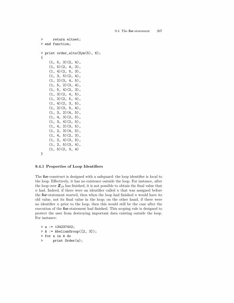
9.4 The for-statement 207
> return eltset;> end function;
> print order_elts(Sym(5), 6);
(1, 5, 3)(2, 4),(1, 5)(2, 4, 3),(1, 4)(2, 5, 3),(1, 3, 5)(2, 4),(1, 2)(3, 4, 5),(1, 5, 2)(3, 4),(1, 5, 4)(2, 3),(1, 3)(2, 4, 5),(1, 3)(2, 5, 4),(1, 4)(2, 3, 5),(1, 2)(3, 5, 4),(1, 3, 2)(4, 5),(1, 4, 3)(2, 5),(1, 3, 4)(2, 5),(1, 4, 2)(3, 5),(1, 2, 3)(4, 5),(1, 4, 5)(2, 3),(1, 2, 4)(3, 5),(1, 2, 5)(3, 4),(1, 5)(2, 3, 4)
9.4.1 Properties of Loop Identifiers
The for-construct is designed with a safeguard: the loop identifier is local tothe loop. Effectively, it has no existence outside the loop. For instance, afterthe loop over ZZ18 has finished, it is not possible to obtain the final value thatn had. Indeed, if there were an identifier called n that was assigned beforethe for-statement started, then when the loop had finished n would have itsold value, not its final value in the loop; on the other hand, if there wereno identifier n prior to the loop, then this would still be the case after theexecution of the for-statement had finished. This scoping rule is designed toprotect the user from destroying important data existing outside the loop.For instance:
> a := 134237402;> A := AbelianGroup([2, 3]);> for a in A do> print Order(a);

208 9. Iterative Statements
> end for;163236> print a;134237402
Similarly, after the loop over G has finished in the permutation groupexample above, it is not possible to obtain the final value that g had, andany identifier g outside the loop is independent of it. This is the case evenwithin the function order elts, but the function itself provides another levelof scope, such that not only g but also eltset have no existence outside thefunction.
Another property of loop identifiers of for-statements is that they maynot be reassigned in the statement body. They exist to be inspected for theircurrent value rather than to be changed by the user. For this reason, loopidentifiers are said to belong to the value class of identifiers.
9.4.2 Using Sequences as Domains of Iteration
If the domain of a for-loop is a sequence (or a list or indexed set), the loopidentifier will run through the elements of the domain in the standard index-ing order. If it is a sequence (or a list or multiset) with repeated elements,then those elements will be assigned to the loop identifier the correspondingnumber of times. For example, the following statement prints each term r ofa sequence of rational numbers, preceded by the floor brc of r (the greatestinteger less than or equal to r):
> for j in [9/2, 1, 3/4, 2, 3/4, 3/4, 54/11] do> print Floor(j), j;> end for;4 9/21 10 3/42 20 3/40 3/44 54/11
The output shows that the terms of the sequence are used in order, includingthe repeated terms.

9.4 The for-statement 209
If the domain of a for-statement is a sequence Q with repeated terms andit is undesirable to repeat the iteration for the same value of the loop identi-fier, then the for-statement should be given the enumerated set Seqset(Q)as its domain. This change can be important when the execution time foreach iteration is non-trivial and the proportion of repeated terms is high.
It often happens that the user wishes the loop identifier to take on thevalues of a range of integers in arithmetic progression: i, i + k, i + 2k, . . . , j.This may be accomplished in Magma by constructing the domain as anarithmetic-progression sequence, using the syntax [i..j by k], or [i..j] if k =1. The procedure on p. 202, which verifies a summation formula, may beencoded with a for-loop instead of a while-loop using this technique:
> testsum := procedure(t)> sum := 0;> for i in [1..t] do> sum +:= i^3;> end for;> print "Equation is", sum eq (t*(t+1) div 2)^2,> "for t =", t;> end procedure;
Notice that the statement i +:= 1; is no longer required, since the for-loop performs the incrementing automatically. The for-statement is the bestiterative statement for this task.
Similarly, the factorial problem on p. 201 can be implemented using afor-statement with an arithmetic-progression sequence as its domain, since cchanges by the constant value −1 on each pass through the loop:
> factl2 := function(n)> error if n lt 0,> "Error in ’factl’: Argument should be >= 0";> answer := 1;> for c in [n..2 by -1] do> answer *:= c;> end for;> return answer;> end function;
The loop identifier c in the for-statement above runs through the integersn, n− 1, . . . down to 2. If n is less than 2 (i.e., n = 1 or n = 0, since n ≥ 0)then the domain sequence is empty. In this case, the statements in the bodyof the for-loop are never executed, so answer retains its initial value of 1,which is the correct value of both 0! and 1!.

210 9. Iterative Statements
9.5 Exiting an Iteration or Loop Quickly
9.5.1 Exiting the Current Iteration Quickly
It sometimes happens within the body of a loop that it is unnecessary toexecute the rest of the statements in the loop body for the current iteration.This often happens when an iterative statement is searching for objects satis-fying certain conditions; once it becomes established that a particular objectdoes not satisfy these conditions, it should be possible to proceed immedi-ately to the next object, in the next iteration. The Magma statement forthis situation is
continue;
When Magma is executing a loop body and encounters this statement, itomits the rest of the statements in the loop body. Execution will proceed tothe next iteration or, if all the iterations have been done, to the statementfollowing the whole loop. For example, the program on p. 206 that prints thesquares in ZZ18 may be modified as follows to use a continue-statement:
> for n in ResidueClassRing(18) do> if not IsSquare(n) then> continue;> end if;> print n;> end for;01479101316
In this case, there is only one statement left in the loop body after thecontinue-statement, so there is no real advantage to the modification. Forlarger loops, continue is useful because it helps avoid a tangle of incompleteif-statements.
9.5.2 Exiting the Whole Loop Quickly
Magma also has a statement

9.5 Exiting an Iteration or Loop Quickly 211
break;
which causes immediate exit from the entire iterative statement. This state-ment is useful in dealing with special cases, or in algorithms that are search-ing for a single value. The following modification of the Fermat conjectureprogram (p. 203) illustrates it:
> n := 1;> repeat> composite := not IsPrime(2^2^n + 1);> if composite then> break;> end if;> n +:= 1;> until n eq 7;> if composite then> print "Conjecture is false, since";> print "(2^2^", n, "+ 1) is composite.";> else> print "Conjecture is true for 1 <= n <= 6.";> end if;Conjecture is false, since(2^2^ 5 + 1) is composite.
It is very appropriate to use the break-statement here because it permits asingle termination condition for the repeat-loop. The previous version hada double exit condition, which is more difficult to handle logically. However,since the iteration operates on the basis of a counter n that is incrementedby 1, a for-statement with a break-statement is an even better choice:
> for n in [1..6] do> composite := not IsPrime(2^2^n + 1);> if composite then> break;> end if;> end for;> if composite then> print "Conjecture is false, since";> print "(2^2^", n, "+ 1) is composite.";> else> print "Conjecture is true for 1 <= n <= 6.";> end if;Conjecture is false, since(2^2^ 5 + 1) is composite.

212 9. Iterative Statements
Now the program is more elegant: it is easier to write, easier to read, anddisplays the logic of the underlying algorithm more clearly. Moreover, thefinal if-statement guarantees that there will be some intelligible output, nomatter what value composite has.
9.5.3 Exits in Nested Loops
If one loop resides within another, it is said to be nested within the largerloop. When Magma encounters
continue;
or
break;
within a nested loop, it assumes that these statements refer to the innermost,smallest loop.
In the case of for-loops, it is possible to override this assumption byspecifying the loop identifier of the relevant loop, after the word continueor break. For example, in the following nested for-loops:
for x in xdomain do...for y in ydomain do
...break x;
...end for;...
end for;
the statement
break x;
refers to the outer loop, so the outer loop will be terminated. If the statementwere
break;
then the inner loop would be terminated.

9.6 Iterations Without Iterative Statements 213
9.6 Iterations Without Iterative Statements
As was stated at the beginning of this chapter, many iterative tasks that haveto be performed with iterative statements in other computer languages mayalso be performed in Magma with set/sequence constructors and associatedoperations. Some of the examples in this chapter will now be implementedwithout using iterative statements, for the sake of comparison.
The identification of the square elements of ZZ18 on p. 206 can be madeshorter and easier to read as follows:
> print [n: n in ResidueClassRing(18) | IsSquare(n)];[ 0, 1, 4, 7, 9, 10, 13, 16 ]
The output has changed from a succession of single integers to a single se-quence, but this may well be preferable anyway. An improvement to theunderlying algorithm may also be made by constructing the squares directly:
> print n^2: n in ResidueClassRing(18); 0, 1, 13, 4, 16, 7, 9, 10
The function returning the set of order–k elements of the permutationgroup G (p. 206) may also be created with a set constructor. By doing this,the return value can be described in a single expression, so the function itselfcan be built with the func-constructor:
> order_elts := func< G, k | g: g in G | Order(g) eq k >;
The operators on sets and sequences can be used in combination withconstructors to produce similarly succinct code. For instance, the verificationof the summation identity on p. 202 may also be done in this way:
> testsum := procedure(t)> sum := &+[ i^3 : i in [1..t] ];> print "Equation is", sum eq (t*(t+1) div 2)^2,> "for t =", t;> end procedure;
The code increases in clarity because the details of the summation processdo not need to be given explicitly by the user.
The factorial program of p. 209 can be encoded similarly, by performingmultiplication on all the elements of a sequence:
> factl3 := function(n)

214 9. Iterative Statements
> error if n lt 0,> "Error in ’factl’: Argument should be >= 0";> return &*[n..2 by -1];> end function;
The above statement works for the n = 0 and n = 1 cases because of aproperty of Magma’s reduction operator. When n = 0 or n = 1, the sequencewhose elements are being multiplied together is empty. Since Magma followsconvention by evaluating an empty product as 1, the result is the correct one.
The testing of a conjecture, such as Fermat’s conjecture (p. 203), can beperformed with forall:
> if forall(ex)n: n in [1..6] | IsPrime(2^2^n + 1) then> print "Conjecture is true for 1 <= n <= 6.";> else> print "Conjecture is false, since";> print "(2^2^", ex, "+ 1) is composite.";> end if;Conjecture is false, since(2^2^ 5 + 1) is composite.
It can be seen that many of the examples in this chapter can be pro-grammed without iterative statements. This does not mean that iterativestatements are always a poor choice, merely that loop examples sufficientlyelementary for illustrative purposes are quite likely to be most clearly encodedin a compact static form.

10. Intrinsics, Signatures and Packages
The functions and procedures which form part of the Magma system areknown as intrinsics. Most of them are system intrinsics, that is, functionsand procedures programmed by the Magma developers and their associates.However, it is also possible for users of Magma to create their own userintrinsics in packages, and attach them to the system in such a way that theyare virtually indistinguishable from system intrinsics. Indeed, it is possiblethat the reader’s version of Magma has been customized in this way, perhapsin a teaching or research context.
Both system intrinsics and user intrinsics are compiled into the Magmainternal pseudo-code, in order to save time when the definition of the intrinsichas to be loaded. When either kind of intrinsic is invoked, type-checking of itsactual arguments is performed, to see that they belong to the correct category.System intrinsics reside permanently in Magma, but user intrinsics can easilybe attached to and detached from the system during a Magma session. Alluser intrinsics are written in the Magma language, in a modified form ofthe syntax for functions and procedures; this syntax is assumed knowledgefor this chapter, and is explained in Chapter 8. By contrast, most of thesystem intrinsics are implemented in the computer language C, but a growingnumber are written in Magma and then permanently attached to the systemby means of the package mechanism described in this chapter.
A moderate quantity of documentation is available for all intrinsics. Thesignature of an intrinsic may be printed, to show the categories of its argu-ments and return values, as well as a brief description. It is possible to listthe signatures of all intrinsics having an argument of category C. The tab-completion facility, which is discussed in Section 15.1, provides for shorthandtyping of all intrinsics. However, only the system intrinsics are explained inthe online help system (see Chapter 11), since that is a form of official docu-mentation provided with Magma that cannot be altered by the inclusion ofuser intrinsics.

216 10. Intrinsics, Signatures and Packages
10.1 Signatures of Intrinsics
The signature of an intrinsic is a short description of the intrinsic, in a fixedformat. First comes the list of its arguments and their categories, then (if itis a function) the list of the categories of its return values, then details ofany parameters it has, and finally a line or two of text describing what theintrinsic does.
The way to obtain the signature of an intrinsic is to print the intrinsic. Forexample, the following line shows how to obtain information about Factorial:
> print Factorial;Intrinsic ’Factorial’
Signatures:
(<RngIntElt> n) -> RngIntElt
The factorial n! for small non-negative n
The signature above states that Factorial has one argument n, in theRngIntElt category (that is, an integer), and that the function returns thefactorial of its argument as an integer.
Some intrinsics can take several kinds of arguments, with respect to theircategories or the number of arguments, so they have several signatures. Forinstance:
> print Rank;Intrinsic ’Rank’
Signatures:
(<AlgMatElt> X) -> RngIntElt(<ModMatRngElt> X) -> RngIntElt
The rank of X
(<ModTupRng> M) -> RngIntElt(<ModMatRng> M) -> RngIntElt
The rank of the free module Mover its base coefficient ring
(<RngUPol> R) -> RngIntElt

10.2 Operators Regarded as Intrinsics 217
(<RngMPol> R) -> RngIntElt(<RngMPolRes> R) -> RngIntElt
The number of indeterminates of Rover its coefficient ring
(<ModLat> L) -> RngIntElt
The rank of the lattice L
(<CurveEll> E) -> RngIntElt
The (lower bound on the) rank of theMordell-Weil group of E;E must be defined over Z
The signatures of Rank show that this function always returns an integer,but that its argument can be: an element of a matrix algebra; an elementof a homomorphism module; a tuple module; a homomorphism module; aunivariate or multivariate polynomial ring or a quotient of such a ring; alattice; or an elliptic curve.
10.2 Operators Regarded as Intrinsics
Operators such as +, # or @ are actually system intrinsics with special syntax.If the operator is enclosed in apostrophe signs, Magma will treat it as if itwere a standard system intrinsic:
> print ’+’(2, 3);5
This technique may be used for obtaining the signature of an operator:
> print ’cat’;Intrinsic ’cat’
Signatures:
(<SeqEnum> s, <SeqEnum> t) -> SeqEnum
Concatenation of the enumerated sequences s and t
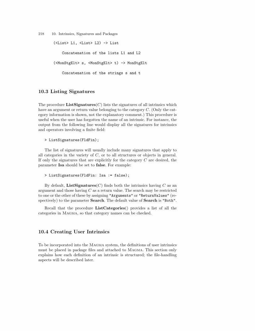
218 10. Intrinsics, Signatures and Packages
(<List> L1, <List> L2) -> List
Concatenation of the lists L1 and L2
(<MonStgElt> s, <MonStgElt> t) -> MonStgElt
Concatenation of the strings s and t
10.3 Listing Signatures
The procedure ListSignatures(C) lists the signatures of all intrinsics whichhave an argument or return value belonging to the category C. (Only the cat-egory information is shown, not the explanatory comment.) This procedure isuseful when the user has forgotten the name of an intrinsic. For instance, theoutput from the following line would display all the signatures for intrinsicsand operators involving a finite field:
> ListSignatures(FldFin);
The list of signatures will usually include many signatures that apply toall categories in the variety of C, or to all structures or objects in general.If only the signatures that are explicitly for the category C are desired, theparameter Isa should be set to false. For example:
> ListSignatures(FldFin: Isa := false);
By default, ListSignatures(C) finds both the intrinsics having C as anargument and those having C as a return value. The search may be restrictedto one or the other of these by assigning "Arguments" or "ReturnValues" (re-spectively) to the parameter Search. The default value of Search is "Both".
Recall that the procedure ListCategories() provides a list of all thecategories in Magma, so that category names can be checked.
10.4 Creating User Intrinsics
To be incorporated into the Magma system, the definitions of user intrinsicsmust be placed in package files and attached to Magma. This section onlyexplains how each definition of an intrinsic is structured; the file-handlingaspects will be described later.

10.4 Creating User Intrinsics 219
User intrinsic functions and user intrinsic procedures are defined in similarways. The syntax for defining a user intrinsic that is a function is:
intrinsic name(argument list) -> return listcomment text
statementsend intrinsic;
and for a user intrinsic procedure it is:
intrinsic name(argument list)comment text
statementsend intrinsic;
The name of the intrinsic may be any identifier. (It may also be a non-alphanumeric collection of characters enclosed in apostrophe signs; this isonly of practical use for extending the use of an existing operator such as +so that it works for some other categories.) If the intrinsic name is alreadythe name of a system or user intrinsic, but the types of the arguments aredifferent, the usages are combined to give multiple signatures.
A function is distinguished from a procedure by having a return list,giving information about the return values. The return list is a list of comma-separated simple types, where a simple type is a category name such asModTupFld (a vector space) or GrphUnd (an undirected graph), a varietyname such as Grp (any group category), a full stop ( . ) indicating ‘any type’,or a pair of brackets indicating a kind of set or sequence ( [], , @@, **,or <> ). The return list is preceded by the characters ->, representing anarrow.
The argument list is a list of comma-separated items that specify thearguments of the intrinsic. For value arguments, the most common kind ofargument specification is name::simple type where the name is an iden-tifier that serves as a formal value argument. Alternatively, the double colonmay be followed by a more general type specification, consisting of brack-eting symbols enclosing a simple type, to indicate the category of the ele-ments of the set or sequence: [simple type], simple type, @simple type@,or *simple type*. For a reference argument of an intrinsic procedure, thesyntax depends on whether the identifier serving as the actual reference argu-ment has to be assigned a value before the procedure is called. If the argumentis expected to have a value already, then ~name::simple type is the ap-propriate syntax. If the argument is not expected to have a value (but will beassigned within the procedure body) then it should be specified as ~namewith no type being given.

220 10. Intrinsics, Signatures and Packages
The comment text, enclosed in braces, is compulsory. It is the sourcefor the textual description of an intrinsic. The statements in the body of thedefinition are normal Magma statements, as would be found in the statementform of a function expression or procedure expression; in the function case,they must include a return-statement with expressions for the return values.
Parameters are permitted in user intrinsics. The syntax is the same asfor user-defined functions/procedures: after the argument list comes a colonand then a list of items of the form parameter := default , giving theparameter name and its default value. There is no category-checking for pa-rameters; it must be done within the body of the intrinsic. The user intrinsicQuadrature given on p. 228 provides an illustration of parameters.
As a simple example of a function intrinsic, consider a conversion of theShuffleGroup(n) function on p. 173. This function takes as its argument aninteger (category RngIntElt) and returns a permutation group (categoryGrpPerm). Therefore the intrinsic is:
intrinsic ShuffleGroup(n::RngIntElt) -> GrpPermThe shuffle group for a deck of 3n cards
m := 3 * n;return PermutationGroup< m |
&*[(i, i + 2 * n) : i in [1 .. n]],&*[(i, i + n, i + 2 * n) : i in [1 .. n]],[((i-1) mod 3)*n + (i-1) div 3 + 1 : i in [1..m]] >;
end intrinsic;
As an example of a procedure intrinsic, the version of EuclideanAlgorithmdefined on p. 178 may be converted as follows:
intrinsic EuclideanAlgorithm(a::RngIntElt, b::RngIntElt)Displays working of Euclidean Algorithmfor gcd of a and b
if a ge b thenA := a; B := b;
elseA := b; B := a;
end if;repeat
q, r := Quotrem(A, B);if r eq 0 then
printf "%o = %o * %o\n", A, q, B;else
printf "%o = %o * %o + %o\n", A, q, B, r;A := B; B := r;
end if;

10.5 Package Files 221
until r eq 0;end intrinsic;
These intrinsics cannot be typed into Magma directly. To be incorporatedinto the system, they must be placed in a package file, and the package filemust be attached to Magma (this has a different effect from that achievedby the load-statement).
10.5 Package Files
A package file is a text file created outside Magma, containing definitions ofuser intrinsics. It may also contain assignment statements, so that constants(including ordinary user-defined functions/procedures) can be defined for useinside the definitions of intrinsics. These constants will not be loaded intothe Magma session; their scope is limited to the package file unless they areexplicitly imported (see Section 10.10). Magma comments are permitted inthe file too.
For example, if a file called mypck1 is created containing the two userintrinsics above, ShuffleGroup and EuclideanAlgorithm, it will be a validpackage file.
As another example, let the following intrinsic functions for string-handling be the contents of the file mypck2. This is another valid packagefile. Notice that it defines the constants STC and R. Constants are usefulwhen programming several related functions or procedures, not only becausethey reduce the amount of typing, but because changes and corrections canbe made more easily.
intrinsic StringToSequence(s::MonStgElt) -> []Sequence of the characters of string s
return [ s[n] : n in [1..#s] ];end intrinsic;
intrinsic SequenceToString(q::[MonStgElt]) -> MonStgEltConcatenation of strings in sequence q
return &* q;end intrinsic;
STC := StringToCode; // shorthandR := STC("A") - STC("a");
intrinsic LowerToUpperCase(s::MonStgElt) -> MonStgElt

222 10. Intrinsics, Signatures and Packages
Convert lower-case alphabetic string s to upper-caseq := [ STC(c) : c in StringToSequence(s) ];return SequenceToString([CodeToString(c + R) : c in q]);
end intrinsic;
intrinsic UpperToLowerCase(s::MonStgElt) -> MonStgEltConvert upper-case alphabetic string s to lower-case
q := [ STC(c) : c in StringToSequence(s) ];return SequenceToString([CodeToString(c - R) : c in q]);
end intrinsic;
10.6 Attaching a Package File
There are several ways of incorporating user intrinsics into Magma. Whilea package file is being developed, the best method is to attach the packageduring the Magma session. After a package has been brought to its finalform and tested, it can be specified along with the user’s other completedpackage files in a spec file (short for ‘specification file’). The spec file may behandled in various ways, to be described later.
The procedure for attaching a package file is Attach(F ), where the file-name is stored in the string F . This string may be a literal string, enclosed in" symbols, or an expression returning a string. If the file is not in the currentdirectory, its absolute or relative path must be given in F . The procedure fordetaching an attached package file during the Magma session is Detach(F ).
For example, suppose that a Magma session is in progress and that thefile mypck1 described above is in the current directory. The package may beattached, and then the intrinsics defined in it become indistinguishable fromsystem intrinsics:
> Attach("mypck1");> print EuclideanAlgorithm;Intrinsic ’EuclideanAlgorithm’
Signatures:
(<RngIntElt> a, <RngIntElt> b)
Displays working of Euclidean Algorithm forgcd of a and b

10.6 Attaching a Package File 223
> EuclideanAlgorithm(133, 24);133 = 5 * 24 + 1324 = 1 * 13 + 1113 = 1 * 11 + 211 = 5 * 2 + 12 = 2 * 1> print ShuffleGroup;Intrinsic ’ShuffleGroup’
Signatures:
(<RngIntElt> n) -> GrpPerm
The shuffle group for a deck of 3n cards
> print ShuffleGroup(5);Permutation group acting on a set of cardinality 15
(1, 11)(2, 12)(3, 13)(4, 14)(5, 15)(1, 6, 11)(2, 7, 12)(3, 8, 13)(4, 9, 14)(5, 10, 15)(2, 6, 12, 14, 10, 4)(3, 11, 9, 13, 5, 7)
When Magma detects an error while attaching a package, it gives anerror message that includes the abbreviation [PC], for ‘package compiler’. Forexample, suppose that the compulsory comment at the top of the intrinsicShuffleGroup had been omitted. When the file was attached, the followingmessage would have been printed:
> Attach("mypck1");[PC][PC] In file "mypck1", line 2, column 5:[PC] >> m := 3 * n;[PC] ^[PC] User error: bad syntax
>> Attach("mypck1");^
Runtime error in ’Attach’: Can’t attach intrinsicsof "mypck1"
When such an error occurs, the file must be corrected and saved. The filemust then be attached, because the previous attempt was unsuccessful.

224 10. Intrinsics, Signatures and Packages
10.7 Changing and Updating a Package File
One of the advantages of user intrinsics over ordinary user-defined functionsis that once a package has been successfully attached to Magma (by anymethod, whether singly or as part of a spec file), Magma automaticallyupdates the intrinsics in the package after a file has been changed and saved.The automatic updating applies both to alterations in existing intrinsics andto new or removed intrinsics. It is not necessary for the user to re-attach thealtered file.
In more detail, just before each top-level statement is executed, Magmacompares the time when the file was last saved with the time when the filewas last processed by the system. If the file has been saved more recently,then the system recompiles the package. This process of time comparison andrecompilation if necessary is called updating a package. Note that the timecomparisons between statements make the operation of the system slightlyslower. To prevent them in cases where the package is stable, the user canplace the command freeze; at the top of the package file, to make a frozenpackage.
Moreover, every time a package (frozen or unfrozen) is attached, Magmaupdates it. The attachment may be by means of Attach, AttachSpec, orthe automatic attachment of spec files at start-up as discussed later in thischapter. Since package attachment normally only occurs once per Magmasession, the time overhead is minimal.
For example, suppose that the file mypck1 is altered so that the procedureEuclideanAlgorithm(a, b) prints the gcd of a and b at the end of the list ofequations. This would require the line
printf "Gcd of %o and %o is %o.\n", a, b, B;
to be placed after the first printf-statement. The following extract of aMagma session indicates how the change would be perceived by the user:
> // file not changed yet> Attach("mypck1");> EuclideanAlgorithm(50, 14);50 = 3 * 14 + 814 = 1 * 8 + 68 = 1 * 6 + 26 = 3 * 2> // file is now edited and saved> EuclideanAlgorithm(50, 14);50 = 3 * 14 + 814 = 1 * 8 + 6

10.8 Testing for Errors in Intrinsics 225
8 = 1 * 6 + 26 = 3 * 2Gcd of 50 and 14 is 2.
Notice that the update of the intrinsic is automatic. It is not necessary tore-attach the altered package. However, if the package had been frozen, thenthis update would not have occurred.
10.8 Testing for Errors in Intrinsics
Recall that the error and error if statements, discussed in Section 8.9, pro-vide a means for a user-defined function or procedure to detect runtime er-rors and stop execution gracefully with an appropriate error message. Thesestatements are also valid in user intrinsics. However, error-checking is slightlyeasier within user intrinsics, for two reasons.
Firstly, since argument types are given in the signatures, arguments of thewrong category are detected immediately. For example, in the package filemypck2, the intrinsic LowerToUpperCase(s) takes a string as its argument.An error message will be given if the argument is not a string:
> Attach("mypck2");> print LowerToUpperCase;Intrinsic ’LowerToUpperCase’
Signatures:
(<MonStgElt> s) -> MonStgElt
Convert lower-case alphabetic string s to upper-case
> print LowerToUpperCase("small");SMALL> print LowerToUpperCase(4/7);
>> print LowerToUpperCase(4/7);^
Runtime error in ’LowerToUpperCase’: Bad argument types
If an argument is an aggregate type, such as a set or sequence, then thecategory of the elements may also be tested. For instance, the intrinsic

226 10. Intrinsics, Signatures and Packages
SequenceToString(q), in the same package file, takes as its argument a se-quence q of strings. It is an error if q is not a sequence or if its elements arenot strings:
> print SequenceToString;Intrinsic ’SequenceToString’
Signatures:
(<SeqEnum[MonStgElt]> q) -> MonStgElt
Concatenation of strings in sequence q
> print SequenceToString(["small", "SMALL", "MeDiUm"]);smallSMALLMeDiUm> print SequenceToString(1234);
>> print SequenceToString(1234);^
Runtime error in ’SequenceToString’: Bad argument types> print SequenceToString([1, 2, 3, 4]);
>> print SequenceToString([1, 2, 3, 4]);^
Runtime error in ’SequenceToString’: Bad argument types
The second reason that error-checking is easier in user intrinsics isthat some special statements are provided for user intrinsics only: require,requirerange, and requirege. They are intended for checking that requiredconditions on the arguments and parameters hold.
The require-statement is the most general, since the user can specify anycondition whose truth is to be tested. The syntax of this statement is:
require condition: expression list;
where the expression list is a list of comma-separated expressions that are tobe evaluated and printed (often the expression list is simply a literal string).If the condition evaluates to true, no action is taken; if it evaluates to false,then execution stops, and Magma prints a message that advises the user ofthe runtime error in the intrinsic and displays the values of the expressions.
The other two statements are only used for an argument or parameterv which takes integer values. The requirerange-statement is used to verifythat v falls within a certain range. It has the syntax:

10.8 Testing for Errors in Intrinsics 227
requirerange v, L, U ;
where L and U are integer expressions. If L ≤ v ≤ U , this statement hasno effect, but otherwise it prints an error message stating the problem. Therequirege-statement is similar:
requirege v, L;
This statement has no effect if v ≥ L, but otherwise it prints an error messagestating the problem.
As an example of the require-statement, observe that in its current formthe intrinsic LowerToUpperCase(s) does not check whether all the charactersof the string s are lower-case:
> print LowerToUpperCase("silly|||STRING");SILLY\[]\\342).’
If LowerToUpperCase is changed to the following intrinsic:
intrinsic LowerToUpperCase(s::MonStgElt) -> MonStgEltConvert lower-case alphabetic string s to upper-case
q := [ STC(c) : c in StringToSequence(s) ];require q subset [STC("a")..STC("z")]:
"String characters must be a, ..., z";return SequenceToString([CodeToString(c + R) : c in q]);
end intrinsic;
then this kind of error will be detected:
> print LowerToUpperCase("silly|||STRING");
>> print LowerToUpperCase("silly|||STRING");^
Runtime error in ’LowerToUpperCase’: String charactersmust be a, ..., z
A similar change should be made to UpperToLowerCase(s).
The intrinsic EuclideanAlgorithm(a, b) would also benefit from a require-statement, to ensure that b 6= 0, since otherwise division by zero would beattempted. The line
require b ne 0:"Argument 2 cannot be 0";

228 10. Intrinsics, Signatures and Packages
should be added after the comment.
The last two examples of intrinsics containing error-detection statementsare modifications of SepLine and quadrature from p. 189 and p. 194 respec-tively. Collectively, they should be understood to be the contents of anotherpackage file, mypck3.
intrinsic SepLine(c::MonStgElt, n::RngIntElt)Prints a line of n copies of string character c
require #c eq 1: "Argument 1 (", c,") should be a single string character";
requirerange n, 0, 80;print c^n;
end intrinsic;
intrinsic Quadrature(f::Program, a::FldPrElt, b::FldPrElt :Al := "Trapezoid", n := 10) -> FldPrElt
Approximate integral of f from a to brequire Category(Al) eq MonStgElt:
"Parameter Al not a string";require Al in "Trapezoid", "Simpson":
"Parameter Al must be \"Trapezoid\" or \"Simpson\"";require Category(n) eq RngIntElt:
"Parameter n not an integer";requirege n, 1;
R := RealField();h := (b - a) / n;if Al eq "Trapezoid" then
return h/2 * ( f(a) + f(b) +2* &+[ R | f(a + k*h): k in [1..(n-1)]] );
else // "Simpson" methodreturn h/3 * ( f(a) + f(b) +
4 * &+[ R | f(a + k*h): k in [1..(n-1) by 2]] +2 * &+[ R | f(a + k*h): k in [2..(n-2) by 2]] );
end if;end intrinsic;
In the first argument of Quadrature, the simple type Program encompassesthe categories Intrinsic (system and user intrinsics) and UserProgram(user-defined functions and procedures), just as the simple types Grp andRng encompass several categories. Observe that parameters do not havetypes given in the signature, so type-checking for them must be done byhand.

10.8 Testing for Errors in Intrinsics 229
Examples of how these intrinsics handle correct and incorrect invocationsare given below:
> Attach("mypck3");> print SepLine;Intrinsic ’SepLine’
Signatures:
(<MonStgElt> c, <RngIntElt> n)
Prints a line of n copies of string character c
> SepLine("#", 20);####################> SepLine("#", -20);
>> SepLine("#", -20);^
Runtime error in ’SepLine’: Argument 2 (-20)should be in the range [0 .. 80]> SepLine("#$", 20);
>> SepLine("#$", 20);^
Runtime error in ’SepLine’: Argument 1 ( #$ )should be a single string character
> print Quadrature;Intrinsic ’Quadrature’
Signatures:
(<Program> f, <FldPrElt> a, <FldPrElt> b) -> FldPrElt[
Al,n
]Approximate integral of f from a to b
> fn := func< x | x^2 + 4/x >;> print Quadrature(fn, 1.0, 10.0);

230 10. Intrinsics, Signatures and Packages
343.67585772176995519638651092653> print Quadrature(fn, 1.0, 10.0 : Al := "Simpson");342.247912047953032217612959374416> print Quadrature(Sin, 2.0, 5.3 : Al := "Simpson");-0.97058595358028565931450853487> print Quadrature(Sin, 2.0, 5.3 : n := 3, Al := "Simpson");0.089229299256145711157092870945> print Quadrature(Sin, 2.0, 5.3 : Al := 33/4);
>> print Quadrature(Sin, 2.0, 5.3 : Al := 33/4);^
Runtime error in ’Quadrature’: Parameter Al not a string> print Quadrature(Sin, 2.0, 5.3 : Al := "junk");
>> print Quadrature(Sin, 2.0, 5.3 : Al := "junk");^
Runtime error in ’Quadrature’:Parameter Al must be "Trapezoid" or "Simpson"> print Quadrature(Sin, 2.0, 5.3 : n := 3.4);
>> print Quadrature(Sin, 2.0, 5.3 : n := 3.4);^
Runtime error in ’Quadrature’: Parameter n not an integer> print Quadrature(Sin, 2.0, 5.3 : n := -300);
>> print Quadrature(Sin, 2.0, 5.3 : n := -300);^
Runtime error in ’Quadrature’: Parameter n should be >= 1
Note also that the arguments that are elements of the real field must beexplicitly supplied by the user as such; integers and rational numbers willnot be coerced automatically into the real field:
> print Quadrature(Sin, 2, 5.3);
>> print Quadrature(Sin, 2, 5.3);^
Runtime error in ’Quadrature’: Bad argument types

10.9 Package Spec Files 231
10.9 Package Spec Files
When a package file or several package files have been tested thoroughly, theyshould be gathered together in a package spec file (‘specification file’), so thatthey can be incorporated as a whole into Magma.
10.9.1 Structure of Spec Files
A package spec file is basically a list of filenames, given in a tree format thatindicates the directory of each file. All the files and directories are describedrelative to the directory in which the spec file is stored.
The simplest form of spec file arises from the situation in which the specfile and all the package files reside in the same directory. In that case, the specfile is a list of all the filenames. The filenames must be separated from oneanother by ‘whitespace’ characters (space, newline, tab); it is conventionalto put them on separate lines. For example, suppose that the package filesare mypck1, mypck2, and mypck3, all in the same directory. If the spec filemyspec is also to be in that directory, then its contents should be:
mypck1mypck2mypck3
In other situations, it is necessary to list directories as well, stating therequired files within the directory. The general rule is that each item in aspec file may be: a filename (as above); or a directory name followed bythe character then a whitespace-separated list of spec file items [recursivedefinition] and then to close off the directory listing.
For example, suppose that there are some additional package files: genlpckin the subdirectory Grp of the directory containing myspec; ord1 and ord2 inthe subdirectory FP of the subdirectory Grp; and other in the subdirectoryMisc of the directory containing myspec. The spec file myspec should nowbe:
mypck1mypck2mypck3Grp
genlpckFP

232 10. Intrinsics, Signatures and Packages
ord1ord2
Misc
other
The indentation is not essential, but it indicates the tree-structure of the specfile to the reader.
10.9.2 Using Spec Files
There are two ways to incorporate the packages in a spec file into Magma:within a session by attaching the spec file, or (semi-)permanently by meansof an environment variable. The first method is for testing the spec file orfor occasional usage (just as one attaches an individual package file), whereasthe second method is employed in order to make the intrinsics in the specfile into part of the user’s standard Magma tools.
The procedure for attaching a spec file is AttachSpec(F ), where thename of the spec file is stored in the string F ; it may be detached during theMagma session with the procedure DetachSpec(F ). The effect of attachinga spec file F is the same as that of attaching all the package files specified inF . For example:
> AttachSpec("myspec");> G := ShuffleGroup(3);> print LowerToUpperCase("tiny");TINY
If the package files are changed, then the package mechanism automaticallyupdates the intrinsics. However, if the spec file is changed there is no updat-ing, so it will need to be detached and re-attached.
There is an environment variable MAGMA USER SPEC which enables the userto attach one or more spec files automatically each time a Magma session iscommenced. This variable should be set to a colon-separated list of the fullpathnames of the spec files. The normal way to do this is to include a linesuch as the following in the user’s .cshrc file:
setenv MAGMA_USER_SPEC "$HOME/Magma/spec:/home/friend/specp"

10.10 Sharing Constants Among Package Files 233
where the two spec files are spec in the user’s Magma directory, and specpin the top directory belonging to the friend. This technique is particularlyuseful when customizing Magma for student purposes, since the modificationis transparent to the user.
Packages that have reached the stage of inclusion in a start-up spec fileshould be made into frozen packages, as explained on p. 224, so as to decreasethe execution time slightly.
10.10 Sharing Constants Among Package Files
Sometimes the same constants (integers, magmas, functions/procedures, etc.)are required by several package files. However, since the scope of objectsassigned in a package file is limited to that file, Magma provides an import-statement so that identifiers can be explicitly referenced from outside thepackage. This technique is designed for the sharing of constants among severalpackages within a spec file, and is preferable to keeping a copy of the constantsin each package.
The syntax of the import-statement, as placed in a package file P , is:
import "filename" : identifier list;
where the identifiers are given in a comma-separated list. The filename iseither absolute or relative to P , and this file must be included in the spec filealong with P , so that it is already attached when the import is performed.The effect of this statement is to create identifiers in the calling context Pwith the same names and values as they have in the named file. If the filewhere the identifiers are assigned is changed later, then automatic updatingtakes place in the context of P .
For example, suppose that the file mydefs is a legal package file, includedin the spec file myspec2. It does not matter for the purposes of this illustrationwhether mydefs contains definitions of intrinsics, but suppose that it includesthe following assignment statements:
Z := IntegerRing();Q := RationalField();R := RealField();
Suppose also that the package file mypck4 is in the same directory as mydefsand is also included in myspec2. If the user wishes to use Z and R but notQ with these meanings within mypck4, then the following statement must beincluded at the top of mypck4:

234 10. Intrinsics, Signatures and Packages
import "mydefs" : Z, R;
After this statement, Z will mean the integer ring and R will mean the realfield when referred to in mypck4. If the values of these identifiers are everchanged in mydefs, this change will flow on to mypck4.

Part III
The User Interface


11. Online Help
Magma is documented in several ways: online help, signatures of intrinsics,hypertext help, and books. This chapter explains how to use Magma’s on-line help system, a mechanism for obtaining help during a Magma session.The online help system includes specially-written material, suitable for near-beginners, and complete access to the descriptions in the Handbook. Most ofthis chapter is devoted to the online help browser, a full subsystem with itsown syntax. However, the browser section is preceded by an overview of howto gain access to the online help system without entering the browser; thisstyle of help request is reviewed later, in the final section.
Section 10.1 and the following sections demonstrated how to find basicinformation about intrinsics, such as the categories of their arguments. Sincethis assistance is obtained during a Magma session, it could be described asonline help, but it is distinct from the online help system proper.
The online help system has a hypertext version called the Magma HTMLHelp Document, which can be read using an Internet browser. The MagmaHTML Help Document is accessed from the shell (the standard interface tothe computer’s operating system), not from within Magma. To read it, theuser should move to a shell prompt and type
magmahelp
If the Magma HTML Help Document can be supported by the computer andhas been installed correctly, an Internet browser will appear, showing thetop node. Since the hypertext help system is self-documenting, it will not bediscussed further here.
The major books on the system are this text, the Handbook [BoC96],and a book entitled Solving Problems with Magma [BCP96] containing longerexamples of Magma code.

238 11. Online Help
11.1 Single Online Help Requests
It is possible to gain access to the online help system without entering thebrowser. This technique is suitable for making one or two simple online re-quests in the midst of a Magma task, whereas the browser is appropriate formore extensive enquiries.
Each single online help request begins with a ? character. If the ? isfollowed by a word, the help system looks for help system nodes referencedby that word. (The referencing is not affected by lower/upper case.) If onlyone node is found satisfying the reference, the online help system shows thatnode:
> ?changedirectory===================================================================PATH: /system/detail/system/ChangeDirectoryKIND: Intrinsic===================================================================ChangeDirectory(s) : MonStgElt ->
Procedure. Change to the directory specified by the string s.‘Tilde expansion’ is allowed.
===================================================================
Otherwise, if several nodes satisfy the reference given after the ?, they arelisted with numbers. To see one of these nodes, the user should type ? followedby its number:
> ?permutation7 matches:
1 O /system/database/perfgps/permutation-representation2 O /system/database/pergps3 S /magma/group/character/Boolean/permutation4 S /magma/group/permutation5 S /magma/group/permutation/Boolean/permutation-group6 S /magma/ring-field-algebra/\
distributive-multivariate-polynomial/group-action/\permutation
7 I /magma/group/permutation/\BSGS-base-strong-generator/operation/Permutation
To view an entry, type ? followed by the number next to it> ?6===================================================================PATH: /magma/ring-field-algebra/polynomial/group-action/permutationKIND: Section===================================================================Permutation Group Actions.
If R is a polynomial ring in n indeterminates x_1, ..., x_n, overany coefficient ring, Sym(n) acts on R by permuting the indices of

11.2 The Online Help Browser System 239
the indeterminates. Thus, the polynomial f(x_1, ..., x_n) ismapped into the polynomial f(x_(g(1)), ..., x_(g(n))).
Intrinsics:
[+1] ^===================================================================
These commands are the basic ones for single help requests. Observe that helprequests do not end with a semicolon, since they are not Magma statements.
If ? is typed alone on a line, information about the help system itself willbe given.
11.2 The Online Help Browser System
The online help browser system permits more extensive and sophisticatedsearches for help than are available through single help requests. To enterthe online help system, the user should type ?? from within Magma:
% magmaMagma V1.10-2 Fri Jul 7 1995 17:03:39 [Seed = 1]Type ? for help. Type <Ctrl>-D to quit.> ??Magma Help BrowserType help for more information??>
Notice that ??> is the special prompt symbol for the browser.
For help about the browser, the user should type help (while in thebrowser). This command, like all other commands in the browser, should notbe followed by a semicolon, since it is not a Magma statement.
The command to leave the browser is quit, exit or control-D.
The browser commands will now be explained. A summary is given inTable 11.1.
11.2.1 The Online Help Nodes
The online help system consists of many help nodes, each of which explainsa feature of the language, the system, or one of the categories. Many ofthe nodes give details of a particular intrinsic as it applies to a magma, orgive an example of such an intrinsic in action. The online help system is

240 11. Online Help
structured as a tree, in which each node (except the root) has a parent noderelating to a more general aspect of the subject. For instance, the parent ofthe node for soluble groups is the node for groups, whose parent is the nodefor magmas, whose parent is the root node. The tree design is similar to thefile hierarchies in many operating systems, except that there is no differencebetween nodes with no children (leaf nodes) and nodes with children, becauseevery node contains text. The command ls (for ‘list’) causes the browser toprint the nodenames of the children of the current node. When the browseris first entered, the current node is the root node, so the output should be asfollows:
??> lsbrowser example language magma system
The command show followed by a nodename displays the contents of thatnode, and show by itself shows the current node. For instance:
??> show system===================================================================PATH: /systemKIND: Overview===================================================================
The Magma system offers several features designed to assistthe user to perform Magma tasks as easily as possible.These include commands for storing Magma information infiles and retrieving it from them, for editing input lines,and for timing computations.
Subnodes (if in Browser, type "w" repeatedly to scan them):
[+1] Magma[+2] control-C-key[+3] database[+4] documentation[+5] history[+6] intrinsic[+7] library[+8] load[+9] prompt[+10] quit[+11] save-restore[+12] shell-escape[+13] signature[+14] time[+15] detail
===================================================================??> show magma===================================================================PATH: /magma

11.2 The Online Help Browser System 241
KIND: Overview===================================================================
The primary concept in the design of the Magma system is that ofa ‘magma’. Following Bourbaki, a magma can be defined asa set with a law of composition.
Thus, types correspond to magmas; a collection of magmas sharing acommon representation forms a category (e.g., the category ofpermutation groups); a collection of categories satisfying the sameset of identical relations forms a variety (e.g., the variety ofgroups). Functors may be used to move between categories, and thevariety operations (substructure, homomorphic image, and Cartesianproduct) are available as uniform constructors across allcategories.
...
Subnodes (if in Browser, type "w" repeatedly to scan them):
[+1] Boolean[+2] aggregate[+3] combinatorial[+4] group[+5] mapping[+6] module[+7] ring-field-algebra[+8] semigroup[+9] string
SEE ALSO:+10 /system/Magma
===================================================================
The command where or pwd prints the current node. To change thecurrent node, the user should type goto or cd followed by the desired node.For instance:
??> whereCurrent node: /??> goto language??> lscategory operatorcomment statementexpression detailfunction-procedure-mapping semanticsidentifier??> goto statement??> whereCurrent node: /language/statement??> show===================================================================

242 11. Online Help
PATH: /language/statementKIND: Overview===================================================================
A statement is a complete command to Magma.Every statement must end with a semicolon ( ; ).
If you press the <return> key before typing ; then Magmamay give you a special prompt symbol such as
print>
or
if>
to remind you that the statement is not yet finished.
EXAMPLE:
> print 5+8;
> DivBy3 := func< n | IsZero(n mod 3) >;
Subnodes (if in Browser, type "w" repeatedly to scan them):
[+1] assignment[+2] case[+3] if[+4] iteration[+5] print
===================================================================
The pathname of each node is given at the top of the output when the nodeis shown. Every pathname begins with the / character. The root node has /as its whole pathname, but every other node has a longer path, indicating itsplace in the tree. Each part of the path is separated from the next by a / sym-bol. For instance, the node in the previous example, /language/statement,is the statement node whose parent is the language node whose parent is theroot node. The command up causes the current node to be changed to itsparent node.
11.2.2 Finding a Node
There are a number of ways to seek help on a particular topic within thebrowser. Although it is possible to perform a series of goto and ls commandsin the hope of finding the goal, this is not the best method unless the user

11.2 The Online Help Browser System 243
is literally browsing and has no idea of the name of the topic. The findcommand is generally preferable:
find word
where the word should be the name of the topic or intrinsic.
The topics in the online help tree have been named with nouns in thesingular, and so find commands should be issued likewise. For example, in-formation about polynomials should be sought using the word polynomial,not polynomials, and information about dividing should be sought usingdivision rather than dividing or divide. However, the online help systemis entirely case-insensitive, so capitals and lower-case letters may be used withidentical results; this is advantageous since the same find command can findboth nodes on topics (section nodes, usually named with lower-case letters)and nodes for intrinsics (usually named with an initial capital). For example:
??> find image8 matches:
1 S /magma/group/matrix/image-orbit-stabilizer2 S /magma/group/permutation/G-set/image-orbit-stabilizer3 S /magma/mapping/detail/image-preimage4 I /magma/group/permutation/G-set/\
image-orbit-stabilizer/Image5 I /magma/mapping/detail/operation/\
domain-kernel/Image6 I /magma/module/homomorphism/operation-element/Image7 I /magma/module/vector-space-linear-transformation/\
linear-transformation/Image8 I /magma/ring-field-algebra/matrix/\
homomorphism-element/ImageTo view an entry, simply type the corresponding number
The output of a find is a numbered list of pathnames. The pathnames suggestthe contents of the node, and therefore indicate which node or nodes probablyapply to the intended help request. For instance, if the command above hadbeen issued in order to research the image of a mapping in Magma, the userwould inspect 3 and 5. Only the numbers themselves need to be typed, sincethe command show may be omitted for a node specified by a number:
??> 3===================================================================PATH: /magma/mapping/detail/image-preimageKIND: Section===================================================================Calculating Images and Preimages.
The standard mathematical notation is used to denote thecalculation of a map image. Some mappings defined by certain
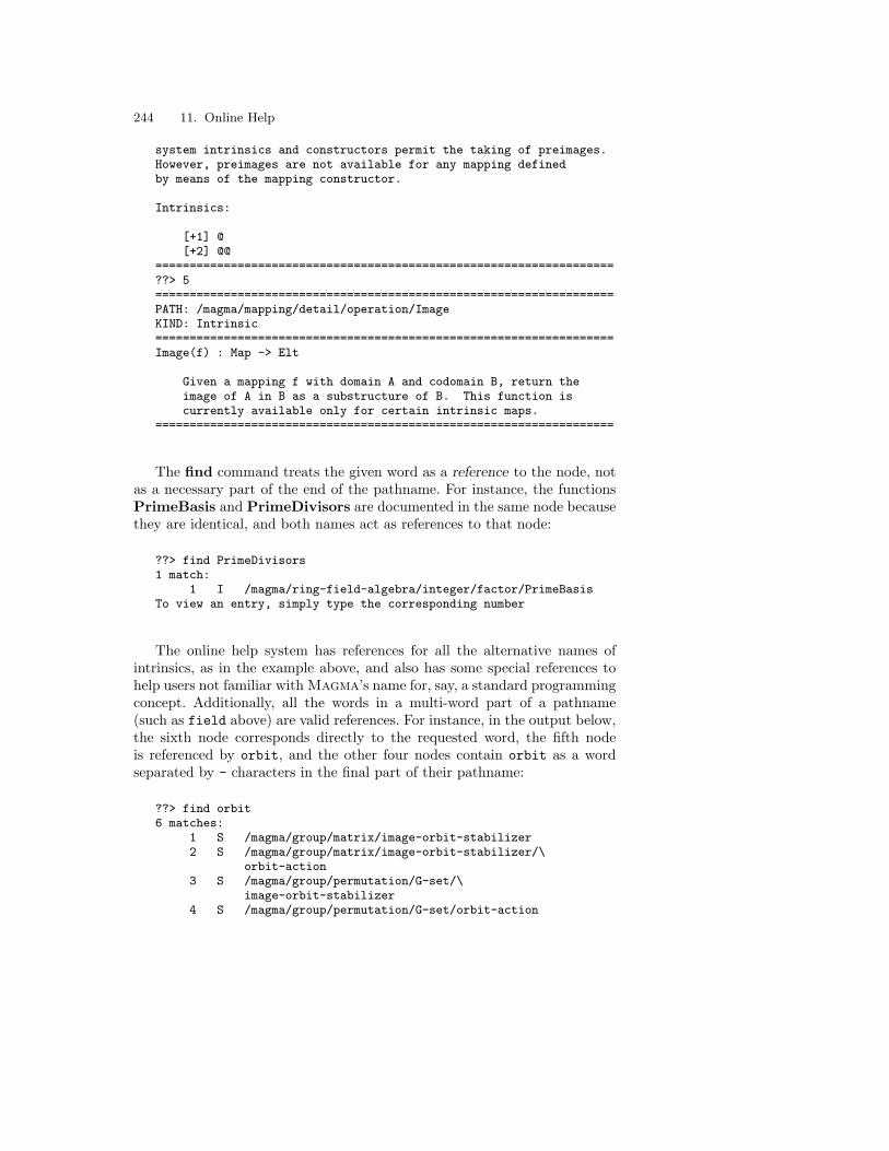
244 11. Online Help
system intrinsics and constructors permit the taking of preimages.However, preimages are not available for any mapping definedby means of the mapping constructor.
Intrinsics:
[+1] @[+2] @@
===================================================================??> 5===================================================================PATH: /magma/mapping/detail/operation/ImageKIND: Intrinsic===================================================================Image(f) : Map -> Elt
Given a mapping f with domain A and codomain B, return theimage of A in B as a substructure of B. This function iscurrently available only for certain intrinsic maps.
===================================================================
The find command treats the given word as a reference to the node, notas a necessary part of the end of the pathname. For instance, the functionsPrimeBasis and PrimeDivisors are documented in the same node becausethey are identical, and both names act as references to that node:
??> find PrimeDivisors1 match:
1 I /magma/ring-field-algebra/integer/factor/PrimeBasisTo view an entry, simply type the corresponding number
The online help system has references for all the alternative names ofintrinsics, as in the example above, and also has some special references tohelp users not familiar with Magma’s name for, say, a standard programmingconcept. Additionally, all the words in a multi-word part of a pathname(such as field above) are valid references. For instance, in the output below,the sixth node corresponds directly to the requested word, the fifth nodeis referenced by orbit, and the other four nodes contain orbit as a wordseparated by - characters in the final part of their pathname:
??> find orbit6 matches:
1 S /magma/group/matrix/image-orbit-stabilizer2 S /magma/group/matrix/image-orbit-stabilizer/\
orbit-action3 S /magma/group/permutation/G-set/\
image-orbit-stabilizer4 S /magma/group/permutation/G-set/orbit-action
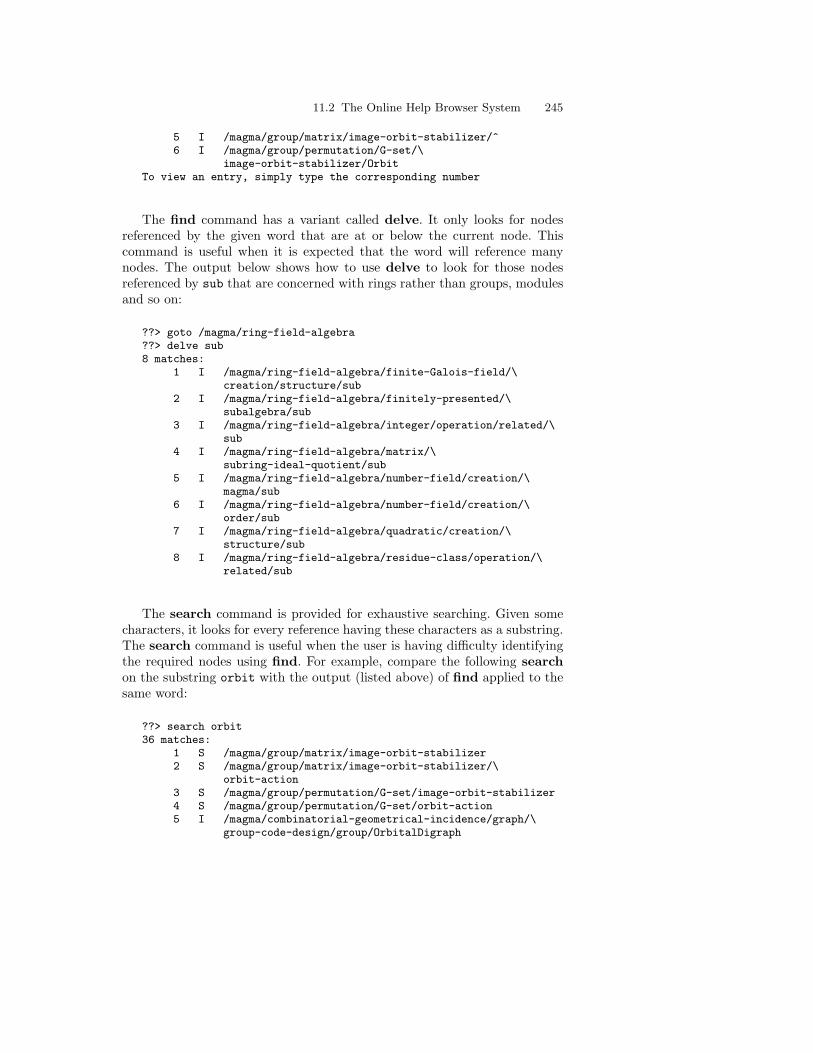
11.2 The Online Help Browser System 245
5 I /magma/group/matrix/image-orbit-stabilizer/^6 I /magma/group/permutation/G-set/\
image-orbit-stabilizer/OrbitTo view an entry, simply type the corresponding number
The find command has a variant called delve. It only looks for nodesreferenced by the given word that are at or below the current node. Thiscommand is useful when it is expected that the word will reference manynodes. The output below shows how to use delve to look for those nodesreferenced by sub that are concerned with rings rather than groups, modulesand so on:
??> goto /magma/ring-field-algebra??> delve sub8 matches:
1 I /magma/ring-field-algebra/finite-Galois-field/\creation/structure/sub
2 I /magma/ring-field-algebra/finitely-presented/\subalgebra/sub
3 I /magma/ring-field-algebra/integer/operation/related/\sub
4 I /magma/ring-field-algebra/matrix/\subring-ideal-quotient/sub
5 I /magma/ring-field-algebra/number-field/creation/\magma/sub
6 I /magma/ring-field-algebra/number-field/creation/\order/sub
7 I /magma/ring-field-algebra/quadratic/creation/\structure/sub
8 I /magma/ring-field-algebra/residue-class/operation/\related/sub
The search command is provided for exhaustive searching. Given somecharacters, it looks for every reference having these characters as a substring.The search command is useful when the user is having difficulty identifyingthe required nodes using find. For example, compare the following searchon the substring orbit with the output (listed above) of find applied to thesame word:
??> search orbit36 matches:
1 S /magma/group/matrix/image-orbit-stabilizer2 S /magma/group/matrix/image-orbit-stabilizer/\
orbit-action3 S /magma/group/permutation/G-set/image-orbit-stabilizer4 S /magma/group/permutation/G-set/orbit-action5 I /magma/combinatorial-geometrical-incidence/graph/\
group-code-design/group/OrbitalDigraph

246 11. Online Help
6 I /magma/combinatorial-geometrical-incidence/graph/\group-code-design/group/OrbitalGraph
7 I /magma/combinatorial-geometrical-incidence/graph/\symmetry-regularity/OrbitsPartition
8 I /magma/group/character/Boolean/conjugate/GaloisOrbit9 I /magma/group/matrix/BSGS-base-strong-generator/\
access/BasicOrbit10 I /magma/group/matrix/BSGS-base-strong-generator/\
access/BasicOrbitLength11 I /magma/group/matrix/BSGS-base-strong-generator/\
access/BasicOrbitLengths12 I /magma/group/matrix/image-orbit-stabilizer/^13 I /magma/group/matrix/image-orbit-stabilizer/LineOrbits14 I /magma/group/matrix/image-orbit-stabilizer/\
orbit-action/OrbitAction15 I /magma/group/matrix/image-orbit-stabilizer/\
orbit-action/OrbitActionBounded16 I /magma/group/matrix/image-orbit-stabilizer/\
orbit-action/OrbitImage17 I /magma/group/matrix/image-orbit-stabilizer/\
orbit-action/OrbitImageBounded18 I /magma/group/matrix/image-orbit-stabilizer/\
orbit-action/OrbitKernel19 I /magma/group/matrix/image-orbit-stabilizer/\
orbit-action/OrbitKernelBounded20 I /magma/group/matrix/image-orbit-stabilizer/\
OrbitBounded21 I /magma/group/matrix/image-orbit-stabilizer/\
OrbitClosure22 I /magma/group/matrix/image-orbit-stabilizer/Orbits23 I /magma/group/permutation/BSGS-base-strong-generator/\
access/BasicOrbit24 I /magma/group/permutation/BSGS-base-strong-generator/\
access/BasicOrbitLength25 I /magma/group/permutation/BSGS-base-strong-generator/\
access/BasicOrbitLengths26 I /magma/group/permutation/BSGS-base-strong-generator/\
access/BasicOrbits27 I /magma/group/permutation/BSGS-base-strong-generator/\
access/IsMemberBasicOrbit28 I /magma/group/permutation/G-set/\
image-orbit-stabilizer/Orbit29 I /magma/group/permutation/G-set/\
image-orbit-stabilizer/OrbitClosure30 I /magma/group/permutation/G-set/\
image-orbit-stabilizer/Orbits31 I /magma/group/permutation/G-set/orbit-action/IsOrbit32 I /magma/group/permutation/G-set/orbit-action/\
OrbitAction33 I /magma/group/permutation/G-set/orbit-action/OrbitImage34 I /magma/group/permutation/G-set/orbit-action/\
OrbitKernel35 E /magma/group/matrix/image-orbit-stabilizer/\

11.2 The Online Help Browser System 247
Example-Orbits36 E /magma/group/permutation/G-set/orbit-action/\
Example-OrbitActions
11.2.3 Walking the Online Help Tree
It is possible to traverse the online help tree step by step. The easiest methodis to goto the node from which the walk will begin, and then type walk (to goforward) or back (to go backward) as many times as required. The followingexample shows how to read about the statements connected with iteration:
??> goto /language/statement/iteration??> lsbreak continue for repeat while??> walk===================================================================PATH: /language/statement/iterationKIND: Overview===================================================================
Magma’s statements while and repeatperform iteration controlled by a Boolean condition.
Another control statement, for , iterates overeach element of some enumerable domain.
...
??> walk===================================================================PATH: /language/statement/iteration/breakKIND: Overview===================================================================
The statement
> break;
inside an iterative statement (loop) causes immediate exit from the...
??> walk===================================================================PATH: /language/statement/iteration/continueKIND: Overview===================================================================
The statement
> continue;

248 11. Online Help
inside a while-statement or repeat-statement causes Magma to omit...
??> walk===================================================================PATH: /language/statement/iteration/forKIND: Overview===================================================================
The for-statement is one of Magma’s iterative statements.It has the syntax:
...
??> back===================================================================PATH: /language/statement/iteration/continueKIND: Overview===================================================================
The statement
> continue;
inside a while-statement or repeat-statement causes Magma to omit...
The current node does not change when a walk or back is performed.The online help system has a separate walk pointer that changes instead.
11.2.4 The Kinds of Help Nodes
There are four kinds of help nodes: Overview (O), Section (S), Intrinsic (I)and Example (E). The online help system states the kind of each node whenit shows its contents, and when it prints it in a list arising from a statementsuch as find. The S, I and E kinds are taken from the Handbook, though someS nodes come from subsections or chapters rather than true chapter-sections.The O nodes are purpose-written for the online help system, so if there is anO node about the user’s topic, it should be read before other nodes on thetopic. Although the O nodes are designed for relative beginners to Magma,they are more terse than the explanations in this book.
It is possible to restrict find, delve, walk and back (as well as search,explained in Table 11.1 (p. 255)) so that they only select one kind of node.The relevant commands are ofind, sfind, ifind, efind, odelve, and so on,with the obvious meanings. For instance, if information is wanted on theintrinsic function Field, then an ifind (a find on I nodes only) is sufficient:
??> ifind field

11.2 The Online Help Browser System 249
2 matches:1 I /magma/combinatorial-geometrical-incidence/\
error-correcting-linear-code/access/Alphabet2 I /magma/combinatorial-geometrical-incidence/plane/\
access/FieldTo view an entry, simply type the corresponding number
The nodes which have been found are the function Field(C) (also calledAlphabet(C)) for a code C, and the function Field(P ) for a classical planeP .
11.2.5 Cross-References
Some nodes give cross-references, indicating nodes directly under the nodebeing read, or whose subject matter is related to this node. They have specialnumbers, beginning with a + symbol. Most cross-references are listed at theend of the contents of the node. For example:
??> show /language/function-procedure-mapping
...
Subnodes (if in Browser, type "w" repeatedly to scan them):
[+1] error[+2] forward[+3] function[+4] procedure[+5] return
SEE ALSO:+6 /language/function-procedure-mapping/function+7 /language/function-procedure-mapping/procedure+8 /magma/mapping+9 /system/intrinsic
===================================================================??> +8===================================================================PATH: /magma/mappingKIND: Overview===================================================================
This section provides an overview of the ideasbehind mappings, including homomorphisms andpartial mappings.
...

250 11. Online Help
A few cross-references are given in the body of the text. These can be readin the same way, by typing the + symbol and the appropriate number. Forinstance, the following lines are contained in the node /language/operator:
All Magma operators use call-by-value evaluation, like theother intrinsics, except the short-circuit operators‘and’, ‘or’, and ‘select’, which use call-by-name evaluation.See [+1].
The reference above could be read by typing +1 at the browser prompt.
11.2.6 Tab Completion in the Browser
On most operating systems, the tab completion feature may be used; compareSection 15.1, which explains tab completion for standard Magma statements.(If tab completion is not available, the best substitute is the search com-mand.) When the tab key is pressed, the browser looks at the word whichthe cursor is on or just after, and considers all the commands, referencesor pathnames (according to the syntax of the command) of which the wordcould be the beginning. If there are no possibilities, there will be a beep. Ifthere is only one possibility, the word will be completed. If there are severalpossibilities, there will be a beep and the word will be expanded as far aspossible, to the end of the common prefix of all the possibilities. In this lastcase, if the tab key is pressed again, the browser will list all of the possiblecompletions, and repeat the input line so that the user can finish it.
For example, the following lines demonstrate how to see the referencesconcerned with prime numbers. The user can then choose some of these nodesto investigate.
??> find Prime [user types 2 tabs]Prime PrimeDivisors PrimeRingPrimeBasis PrimeFieldPrimeCertificate PrimeForm??> find Prime
When employing the tab completion feature, the user should type as lit-tle as possible of the beginning of the word, so as not to miss anythingrelevant. For instance, the reference Primality might also be of interest inthe example above, but it was not found because it did not begin with prime(case-insensitive). The following command would have found it:
??> find Prim [user types 2 tabs]Primality PrimeDivisorsprimality PrimeField

11.2 The Online Help Browser System 251
Primary PrimeFormPrimaryDecomposition PrimeRingPrimaryInvariantFactors primitivePrimaryInvariants PrimitiveElementPrimaryRationalForm PrimitivePartPrime PrimitivePolynomialPrimeBasis PrimitiveRootPrimeCertificate PrimitiveStructure??> find Prim
However, some of these references are not associated with prime numbers.There is a trade-off between obtaining all the relevant references and notobtaining an excessive number of irrelevant references.
A series of tab completions on a pathname may be used in a kind of inlinebrowsing, with very few keystrokes required. For example:
??> show / [user types 2 tabs]browser example language magma system??> show /m [user types tab]
... above line becomes:??> show /magma [user types tab]
... above line becomes:??> show /magma/ [user types tab]
... above line becomes:??> show /magma/ [user types 2 tabs]Booleanaggregatecombinatorial-geometrical-incidencegroupmappingmodulering-field-algebrasemigroupstring??> show /magma/g [user types 4 tabs]
... above line becomes:??> show /magma/group/group-overview soluble characterabelian permutationfinitely-presented matrix??> show /magma/group/m [user types 4 tabs]introductioncreation-general-linear-groupoperation-elementcreation-general-matrix-groupextension-standard-groupchange-ringoperationelementimage-orbit-stabilizeroperation-subgroup

252 11. Online Help
Booleancharacteristic-subgroup-normal-structureconjugatesoluble-matrix-groupcharacter-representationBSGS-base-strong-generator??> show /magma/group/matrix/b [user types 2 tabs]
... above line becomes:??> show /magma/group/matrix/BBoolean BSGS-base-strong-generator??> show /magma/group/matrix/Bo [user types 4 tabs]
... above line becomes:??> show /magma/group/matrix/Boolean/matrix-group abstract-group??> show /magma/group/matrix/Boolean/a [user types 4 tabs]
... above line becomes:??> show /magma/group/matrix/Boolean/abstract-group/IsIsAbelian IsNormalIsCyclic IsPerfectIsElementaryAbelian IsSelfNormalizingIsCentral IsSimpleIsConjugate IsSolubleIsMaximal IsSubnormalIsNilpotent??> show /magma/group/matrix/Boolean/abstract-group/Is
...
11.2.7 Recalling Nodes
The command numbers reprints the list of nodes from the most recentfind, delve or search command. It is helpful when the user has looked atthe contents of some nodes in such a list and has forgotten the numbers ofthe other nodes.
Another way of keeping track of useful nodes is to mark them for laterreading. The following example shows how to mark the nodes connected withcyclic linear codes:
??> search cyclic18 matches:
1 S /magma/combinatorial-geometrical-incidence/\error-correcting-linear-code/creation/cyclic
2 S /magma/group/soluble/introduction/\polycyclic-power-conjugate
3 I /magma/combinatorial-geometrical-incidence/\error-correcting-linear-code/Boolean/IsCyclic
4 I /magma/combinatorial-geometrical-incidence/\error-correcting-linear-code/creation/cyclic/\CyclicCode

11.2 The Online Help Browser System 253
5 I /magma/group/abelian/group-Boolean/IsCyclic6 I /magma/group/finitely-presented/\
extension-standard-group/standard/CyclicGroup7 I /magma/group/group-overview/creation-general/magma/\
Group8 I /magma/group/group-overview/extension-standard-group/\
standard/CyclicGroup9 I /magma/group/group-overview/operation-subgroup/\
abstract-group/IsCyclic10 I /magma/group/matrix/Boolean/abstract-group/IsCyclic11 I /magma/group/matrix/soluble-matrix-group/conversion/\
PolycyclicGenerators12 I /magma/group/permutation/Boolean/abstract-group/\
IsCyclic13 I /magma/group/permutation/extension-standard-group/\
standard/CyclicGroup14 I /magma/group/soluble/creation-element/magma/\
PolycyclicGroup15 I /magma/group/soluble/group-Boolean/IsCyclic16 I /magma/group/soluble/subgroup-quotient-extension/\
standard-group/CyclicGroup17 E /magma/combinatorial-geometrical-incidence/\
error-correcting-linear-code/creation/cyclic/\Example-CyclicCode
18 E /magma/group/soluble/creation-element/magma/\Example-PolycyclicGroup
??> mark 1[’1] S /magma/combinatorial-geometrical-incidence/\
error-correcting-linear-code/creation/cyclic??> mark 3[’2] I /magma/combinatorial-geometrical-incidence/\
error-correcting-linear-code/Boolean/IsCyclic??> mark 4[’3] I /magma/combinatorial-geometrical-incidence/\
error-correcting-linear-code/creation/cyclic/CyclicCode??> mark 17[’4] E /magma/combinatorial-geometrical-incidence/\
error-correcting-linear-code/creation/cyclic/\Example-CyclicCode
Now these nodes will have the special node specifications ’1, ’2, ’3 and ’4.For example:
??> ’3===================================================================PATH: /magma/combinatorial-geometrical-incidence/\
error-correcting-linear-code/creation/cyclic/CyclicCodeKIND: Intrinsic===================================================================CyclicCode(u) : ModTupFldElt -> Code
Given a vector u belonging to the K-space K^((n)), construct

254 11. Online Help
the [n, k] cyclic code generated by the right cyclic shifts ofthe vector u.
CyclicCode(n, g) : RngIntElt, RngUPolElt -> Code
Let K be a finite field. Given a positive integer n and aunivariate polynomial g(x) in K[x] of degree n - k such thatg(x) | x^n - 1, construct the [n, k] cyclic code generatedby g(x).
===================================================================
The command marks lists the marked nodes:
??> marks’1 S /magma/combinatorial-geometrical-incidence/\
error-correcting-linear-code/creation/cyclic’2 I /magma/combinatorial-geometrical-incidence/\
error-correcting-linear-code/Boolean/IsCyclic’3 I /magma/combinatorial-geometrical-incidence/\
error-correcting-linear-code/creation/cyclic/\CyclicCode
’4 E /magma/combinatorial-geometrical-incidence/\error-correcting-linear-code/creation/cyclic/\Example-CyclicCode
The browser system will remember these marks for the rest of the Magmasession, even if the user quits the browser and does some Magma computa-tions before re-entering the browser.
The command unmark followed a mark number removes that mark fromthe list of marks.
11.2.8 Summary of Browser Commands
Table 11.1 summarizes the online help system browser commands, but omitsthe prefixed versions of the commands, such as efind and odelve. In thetable, n denotes a node specification, which may be any of: an absolutepathname; a pathname relative to the current node (e.g., iteration/whilewhen the current node is /language/statement); an integer in the currentnumbers range; the character + and a integer within the current cross-reference range; the character ’ and a integer within the current marks range;or the character ", indicating the last node to which the user referred.
Every browser command may be abbreviated to a substring with whichit begins. If more than one command begins with the given substring, thebrowser interprets it as the command that comes first alphabetically. (Ex-ceptions are s for show and e for exit.) For example, some command abbre-

11.3 Other Features of Single Online Help Requests 255
Table 11.1. Online help system browser commands
Magma Meaning
?? Enter the online help system browser
quit, exit, control-D Leave the browser
help Help about browser (node /browser)
? Help about help system (root node /)
show, cat, more Display text of current node
show n, cat n, more n Display text of help node specified by n
where, pwd State current node
ls List children of current node
ls n List children of n
goto, cd Change current node to root node /
goto n, cd n Change current node to n
up Change current node to parent of current node
up n Change current node to parent of n
walk, back Go forward/backward with respect to walk pointer
walk n, back n show n, and set walk pointer to it
find w List nodes referenced by word w
delve w List nodes referenced by word w that are beneathcurrent node in the help tree
search s List nodes whose references contain substring s
numbers Reprint list from most recent find, delve or search
i show i, where i ∈ ZZ is a node specification
mark n Mark n (or current node, if n omitted) for futurereference; n will get a node specification ’i, wherei ∈ ZZ
unmark m Remove mark m from marks list
marks m List the marks list
viations are d (delve), f (find), iw (walk along the intrinsics) and sb (backalong the sections).
11.3 Other Features of Single Online Help Requests
A single help request, that is, one beginning with a ? character, is rather likefind or show in the browser. If the ? is followed by a reference word, thenthe system performs a find. In the case that there is exactly one match, ashow is performed as well. The ? may also be followed by a full pathname, anumber, or a cross-reference. In these cases, it performs a show. For example:
> ?/system/time

256 11. Online Help
===================================================================PATH: /system/timeKIND: Overview===================================================================
Magma has a mechanism for measuring how long ittakes to execute a statement or statements.
...
===================================================================>
Single help requests (i.e., those starting with ?) may be made within thebrowser, but they operate somewhat independently from the browser. Forinstance, they do not change the value of ", the last-node character.
Tab completion is available following ?, although only outside the browser.This facility greatly enhances the usefulness of single online help requests fromthe Magma level, especially for users who are accustomed to the structureof the online help system tree.

12. Strings
Strings are strongly associated with Magma input and output, but theyalso belong to a magma in their own right, the string structure. The cate-gory of this structure is the character string monoid. The fundamental stringoperations are concatenation and indexing, and thus they share some op-erations with other monoids and with sequences. Sophisticated operationsfor the analysis of strings are provided, including the matching of regularexpressions.
12.1 Creating a String
It has already been seen in this book that Magma allows text – letters andany other characters – to be part of the output of a print-statement. Forexample:
> print "The result of 6 times 7 is", 6 * 7;The result of 6 times 7 is 42
Text like this is called a string, and it is composed of characters (T, h, e,the space character, r, etc.). When a literal string is typed into Magma, thecharacters must be enclosed in " symbols (double quotation marks).
Like any other values, strings can be assigned to identifiers. For instance,if the above line is rewritten as
> ResultStr := "The result of 6 times 7 is";> print ResultStr, 6 * 7;The result of 6 times 7 is 42
then the output is the same.
Every character in a string is significant, even the spaces. For instance:
> AreEqualStrings := ResultStr eq "Theresultof6times7is";

258 12. Strings
> print AreEqualStrings;false
All strings have the same parent, the string structure; the functionStrings() returns this magma. The category of the string structure isthe character string monoid, MonStg, and the category of each string isMonStgElt.
12.2 Operations on Strings
Table 12.1. Operations on strings
Magma Meaning
#s Length of string s
s*t, s cat t String formed by concatenating s and t
s^n s* · · · *s (n copies concatenated)
Position(s, t), Index(s, t) First character position of s at which a copy oft starts, or zero if t not a substring of s; if t isempty, always returns 1
s[i] The length-1 string which is the ith character ofstring s
Substring(s, n, k) Substring of s starting at position n with lengthk (or extending to end of string, if k > #s−n+1)
s eq t true if string s is equal to string t
s ne t true if s is not equal to t
s in t true if s is a contiguous substring of t
s notin t true if s not a contiguous substring of t
s gt t true if s comes later than t (with respect to thestandard lexicographic ordering)
s ge t true if s equals t or comes later than t
s lt t true if s comes earlier than t
s le t true if s equals t or comes earlier than t
The character string monoid is so named because it is a monoid in thesense of semigroup theory. The main operation for strings is concatenation,and the identity of the string structure is the empty string (the string withzero characters). The concatenation operator may be typed as the * symbol,and ^ has a corresponding function as an exponentiation operator.
On the other hand, because concatenation and the position of charactersin strings are important operations for strings, several of the string operators
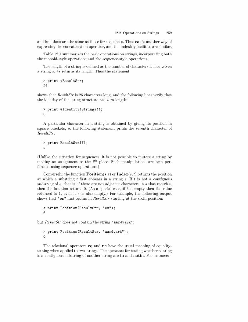
12.2 Operations on Strings 259
and functions are the same as those for sequences. Thus cat is another way ofexpressing the concatenation operator, and the indexing facilities are similar.
Table 12.1 summarizes the basic operations on strings, incorporating boththe monoid-style operations and the sequence-style operations.
The length of a string is defined as the number of characters it has. Givena string s, #s returns its length. Thus the statement
> print #ResultStr;26
shows that ResultStr is 26 characters long, and the following lines verify thatthe identity of the string structure has zero length:
> print #Identity(Strings());0
A particular character in a string is obtained by giving its position insquare brackets, so the following statement prints the seventh character ofResultStr :
> print ResultStr[7];s
(Unlike the situation for sequences, it is not possible to mutate a string bymaking an assignment to the ith place. Such manipulations are best per-formed using sequence operations.)
Conversely, the function Position(s, t) or Index(s, t) returns the positionat which a substring t first appears in a string s. If t is not a contiguoussubstring of s, that is, if there are not adjacent characters in s that match t,then the function returns 0. (As a special case, if t is empty then the valuereturned is 1, even if s is also empty.) For example, the following outputshows that "es" first occurs in ResultStr starting at the sixth position:
> print Position(ResultStr, "es");6
but ResultStr does not contain the string "aardvark":
> print Position(ResultStr, "aardvark");0
The relational operators eq and ne have the usual meaning of equality-testing when applied to two strings. The operators for testing whether a stringis a contiguous substring of another string are in and notin. For instance:

260 12. Strings
> print "om" in "computational";true> print "magma" notin "volcano";true
Strings may be composed from smaller strings by concatenation, usingthe * operator (or the operator cat, which behaves in the same way). Forinstance:
> L := "left";> R := "right";> LR := L cat " " cat R;> print LR;left right> print LR eq (L * " " * R);true
The mutation assignment operators cat:= and *:= are available, as are thereduction operators &cat and &*.
The ^ operator relates to * in the same way as it does for integers ormonoid elements. Given a string s and a non-negative integer n, s^n returnsthe concatenation of n copies of s. For instance, the following lines constructfour cycles of a marching call:
> LRsp := LR * " ";> marching := LRsp ^ 4;> print marching;left right left right left right left right
The operators lt, le, gt, and ge compare two strings with respect to al-phabetical order. (More exactly, these operators refer to lexicographic order-ing, according to the character code used by the computer system on whichMagma is running; for most systems it will be the ASCII character set.) Forinstance, the statement below prints the value false, because ‘xylophone’comes ahead of ‘yacht’ in dictionary order:
> print "xylophone" gt "yacht";false
As a longer illustration of the string operations, suppose that a sentencesuch as ‘There is a chair.’ or ‘There are some books.’ is to be printed, basedon the value of a noun such as ‘chair’ or ‘books’. The following procedure willperform this task:
> Sentence := procedure(Noun)

12.3 Special Characters in Strings 261
> VerbArticle := Noun[#Noun] eq "s" select> " are some " else " is a ";> print "There" * VerbArticle * Noun * ".";> end procedure;
The procedure works well for most sensible input, but fails for singular nounsthat begin with a vowel:
> Sentence("chair");There is a chair.> Sentence("books");There are some books.
> Sentence("egg");There is a egg.
A modification can be made to cater for this case:
> Sentence := procedure(Noun)> if Noun[#Noun] eq "s" then> Verb := " are ";> Article := "some ";> else> Verb := " is ";> if Noun[1] in "aeiouAEIOU" then> Article := "an ";> else> Article := "a ";> end if;> end if;> print "There" * Verb * Article * Noun * ".";> end procedure;
> Sentence("egg");There is an egg.
While this modification is simple, it is harder to write a procedure which willcope with nouns such as ‘boss’ and ‘women’, for which having a final ‘s’ isnot equivalent to being plural. Regrettably, it is not so easy to teach humanlanguages to computers.

262 12. Strings
Table 12.2. Special characters in strings
Magma Meaning
\t Tab character
\n, \r New-line or return character
\" Double quotation mark character
\\ Backslash character
\<return> Line continuation (ignored)
12.3 Special Characters in Strings
There are some characters that it is not possible to obtain straightforwardlyat the keyboard. These characters can be included in strings by using a specialsymbol beginning with a backslash. Table 12.2 lists them.
Tab characters and newlines are useful for manipulating the presentationof output. For instance:
> print "Tab is soon\tThere it was\nsecond line now";Tab is soon There it wassecond line now
To include the " character in a string without having Magma think thatthe string has finished, it must be preceded by a backslash. To obtain thebackslash character itself, it must also be typed with an extra backslash:
> print "a double quotation mark \" and\ra backslash \\";a double quotation mark " anda backslash \
There is a related device called line continuation that is useful for longinput lines. If a backslash is followed immediately by the ‘return’ key, Magmawill provide a newline on the keyboard but will ignore both the backslash andthe ‘return’ internally. For example:
> print "This could well be described as an extreme\> ly long line";This could well be described as an extremely long line
Line continuation works outside strings as well, and so it can be used for longnumerical input or for presentations of large magmas:
> print 123456789012345678901234567890\

12.4 Analysis of Strings 263
> 1234567890;1234567890123456789012345678901234567890
12.4 Analysis of Strings
12.4.1 String Conversions
Sophisticated operations on a string, such as changing parts of it, reorderingit, or seeing how often the same character appears in it, are best done byconverting the string into a sequence first. Sequence operations are explainedin Chapter 6. The following lines show some Magma functions for convertingbetween a string and the sequence of its characters in the same order. Theyuse a sequence constructor, string indexing, and the reduction operator forconcatenation:
> StringToSequence := func< s | [ s[n] : n in [1..#s] ] >;> SequenceToString := func< q | &* q >;> // define abbreviations as well> Strseq := StringToSequence;> Seqstr := SequenceToString;
For example:
> Str := "asdliua0987tas";> Sq := StringToSequence(Str);> print Sq;[ a, s, d, l, i, u, a, 0, 9, 8, 7, t, a, s ]> print SequenceToString(Sq);asdliua0987tas
There are several intrinsics for more specialized conversions. The func-tions IntegerToString(n) and StringToInteger(s) convert an integer intoa string, and an integer-string into an integer. Here an integer-string is astring that consists entirely of digits, except that the first character may bea + or - character. For example:
> s := "-05663"; print StringToInteger(s);-5663
A related function is StringToIntegerSequence(s), which takes a string sconsisting of integer-strings, and returns a sequence of integers correspond-ing to these integer-strings. The integer-strings must be separated from oneanother by one or more spaces, or by an initial + or - sign:

264 12. Strings
> print StringToIntegerSequence("1234 -58 +04-283");[ 1234, -58, 4, -283 ]
It is possible to convert between a one-character string and the charactercode that it has in the computer’s operating system, using CodeToString(n)and StringToCode(s). For most systems on which Magma is running, thiswill be the ASCII character code. The following example, which assumes anASCII context, converts a string of lower-case letters into the correspondingstring of upper-case (capital) letters:
> LowerToUpperCase := function(s)> STC := StringToCode; // shorthand> q := [ STC(c) : c in Strseq(s) ];> error if q notsubset [STC("a")..STC("z")],> "Runtime error in LowerToUpperCase:",> "String characters must be a, ..., z";> R := STC("A") - STC("a");> return Seqstr([ CodeToString(c + R) : c in q ]);> end function;
> print LowerToUpperCase("MAGMA");Runtime error in LowerToUpperCase: String charactersmust be a, ..., z> print LowerToUpperCase("magma");MAGMA
See p. 221 and p. 227 for the implementation of these functions as userintrinsics.
12.4.2 Splitting into Substrings
Given strings s and d, the function Split(s, d) splits s into a sequence ofsubstrings, where the separation points are the places in s at which one ormore of the characters in d occur one or more times. The characters in thedelimiter string d (such as a space, a newline, a tab, a comma, or a colon) arenot included in the substrings in the resulting sequence. More precisely, if sis of the form s1d1s2d2 · · · dk−1sk or s1d1s2d2 · · · dk−1skdk where the stringssi and di are all non-empty (except possibly s1) such that all the charactersof each di are in d and none of the characters of any si are in d, then thefunction returns the sequence [s1, . . . , sk]. As an exception, if s is empty thenthe function returns an empty sequence.
For example, the following invocation of Split takes a string str consistingof letters and digits, and constructs the letter-only substrings of str that areseparated by digits:

12.4 Analysis of Strings 265
> str := "qj23jk259xvnsd9832h34r98723un5kj";> print Split(str, "1234567890");[ qj, jk, xvnsd, h, r, un, kj ]
The next example illustrates how to use whitespace (spaces, tabs, and new-lines) as the delimiter:
> str2 := "The quick brown fox\tjumps> over a lazy\t\t\tdog";> print str2;The quick brown fox jumpsover a lazy dog> print Split(str2, " \t\n");[ The, quick, brown, fox, jumps, over, a, lazy, dog ]
There is an alternative form of this function, Split(s), which splits thestring s into its distinct lines. That is, it uses the newline character as thedelimiter d. For instance, str2 above would be split into two lines:
> print Split(str2);[ The quick brown fox jumps,over a lazy dog ]
12.4.3 Regular Expressions
The function Regexp(r, s) analyzes the string s according to the regular ex-pression given by the string r. Its principal return value is true, if s matches r,else false. If the first return value is true, it returns two additional values: thesubstring of s that was found to match r, and the sequence of matched sub-strings of s corresponding to the parenthesized expressions of r. The meaningof these return values is explained below.
The regular expression r is used to describe a pattern that may be satisfiedby a substring of s. Apart from literal characters, it may contain any of thespecial symbols listed in Table 12.3. For example:
> str3 := "quick brown fox";> m, ss := Regexp("ui.*o", str3);> print m;true> print ss;uick brown fo
> m, ss := Regexp("[ e-z]*$", str3);

266 12. Strings
Table 12.3. Special characters in regular expressions
Magma Meaning
a|b String a or string b
a* Zero or more copies of a
a+ One or more copies of a
a? Zero or one copies of a
^a String a at the beginning of the expression
a$ String a at the end of the expression
. Any character
[c1 · · · ck] Any single character ci
[^c1 · · · ck] Any single character except one of the ci
[c1-ck] Any single character in the range c1 to ck, according to the ma-chine character code (e.g., consecutive letters or digits)
[^c1-ck] Any single character not in the range c1 to ck
\c Character c as a literal, without its special meaning (used forcharacters in this table)
(a) Grouping symbol to restrict scope; a will be a term of the se-quence given as the third return value of Regexp
> print m;true> print ss;rown fox
If some parts of r are enclosed in parentheses, there will be two effects. Firstly,it will restrict the scope of that part of the expression. Secondly, each sectionof the matched substring corresponding to a parenthesized portion of r willbe returned in a sequence, in order from left to right, as the third returnvalue of Regexp. For instance:
> print Regexp("u(i.)*o", str3);false
> print Regexp("[a-z]([a-z]*)[a-z] (.)[a-z]*(.) ", str3);true quick brown [ uic, b, n ]
The final example uses Regexp and Pipe (see Section 14.8.2) to extractinformation about the date from the output of the UNIX command date:
> date := Pipe("date\n", "");> print date;Tue Jul 23 14:31:14 EST 1996

12.4 Analysis of Strings 267
> _, ss, q :=> Regexp(" (.*) ([0-9][0-9]?) .*EST (....)", date);> print ss;Jul 23 14:51:53 EST 1996
> print q;[ Jul, 23, 1996 ]> month, day, year := Explode(q);> printf "Today is %o %o %o.", day, month, year;Today is 23 Jul 1996.
For more details about Regexp, refer to documentation for the freelydistributable reimplementation of the V8 regexp package by Henry Spencer,on which Regexp is based.


13. Printing and User Input
13.1 Levels of Printing in the print-statement
The most common syntax for the print-statement in Magma is:
print expression, . . . , expression;
where the word print may be omitted if the statement is not within a functionor procedure definition. It prints the values of the expressions, in order. Ifthere is more than one expression, the values may be printed on new lines,depending on the categories of the values.
There is also a more general form of the print-statement, that specifiesthe kind of output required:
print expression, . . . , expression : level;
There are four possibilities for the level: Minimal, Default, Maximal andMagma. The first three of these options specify the quantity of the output,from the least to the greatest (though for many categories, two or three ofthe levels produce the same quantity of output). If the colon and the level areomitted entirely, as shown in the first version of the syntax above, then theDefault level is used. The level Magma specifies that the output is to bein Magma-readable format; that is, it should be possible to copy the outputand paste it into Magma as an expression that evaluates to the same value.
For example:
> F3 := GF(3);> MR := MatrixRing< F3, 2 | [2,1,1,0] >;> print MR;Matrix Algebra of degree 2 with 1 generator over GF(3)> print MR : Magma;MatrixAlgebra<GF(3, 1), 2 | [ 2, 1, 1, 0 ]>

270 13. Printing and User Input
> A4 := Alt(4);> print A4;Permutation group A4 acting on a set of cardinality 4Order = 12 = 2^2 * 3
(1, 2)(3, 4)(1, 2, 3)
> print A4 : Minimal;GrpPerm: A4
> D := Design< 3, 5 | Setseq(Subsets(1..5, 3)) >;> print D;3-(5, 3, 1) Design with 10 blocks> print D : Maximal;3-(5, 3, 1) Design with 10 blocksPoints: @ 1, 2, 3, 4, 5 @Blocks:
1, 3, 5,2, 3, 4,1, 4, 5,2, 4, 5,1, 2, 5,1, 2, 3,1, 2, 4,3, 4, 5,2, 3, 5,1, 3, 4
> print D : Magma;Design< 3, @ IntegerRing() | 1, 2, 3, 4, 5 @ |KMatrixSpace(GF(2), 5, 10) ! [ 1, 0, 1, 0, 1, 1, 1, 0, 0,1, 0, 1, 0, 1, 1, 1, 1, 0, 1, 0, 1, 1, 0, 0, 0, 1, 0, 1,1, 1, 0, 1, 1, 1, 0, 0, 1, 1, 0, 1, 1, 0, 1, 1, 1, 0, 0,1, 1, 0 ] : Check := false >
13.2 Printing an Object to a String
The output obtained when printing an expression x may be obtained as astring by means of the Sprint function. Any of the levels in the print-statement may be specified.
For the default level of printing, Sprint(x) returns a string whose valueis the output that would be given by a print x; statement. For example:
> str := Sprint(Alt(4));

13.3 Verbose Printing 271
> print #str;94> print str;Permutation group acting on a set of cardinality 4Order = 12 = 2^2 * 3(1, 2)(3, 4)(1, 2, 3)> _, _, ordq := Regexp("Order = (.*) =", str);> ord := Rep(ordq); print ord;12
For the other levels of printing, suppose that L is any of the strings"Minimal", "Default", "Maximal", or "Magma". Then Sprint(x, L) returnsa string whose value is the output that would be given by printing x withthe corresponding level. For example, parts of the Magma description of adesign may be extracted (as strings):
> D := Design< 3, 5 | Setseq(Subsets(1..5, 3)) >;> str2 := Sprint(D, "Magma");> print str2;Design< 3, @ IntegerRing() | 1, 2, 3, 4, 5 @ |KMatrixSpace(GF(2), 5, 10) ! [ 1, 0, 1, 0, 1, 1, 1, 0, 0,1, 0, 1, 0, 1, 1, 1, 1, 0, 1, 0, 1, 1, 0, 0, 0, 1, 0, 1,1, 1, 0, 1, 1, 1, 0, 0, 1, 1, 0, 1, 1, 0, 1, 1, 1, 0, 0,1, 1, 0 ] : Check := false >> _, _, q := Regexp(> "([0-9]*), (@.*@).*(KMatrixSpace.*) : Check", str2);> t, pts, blks := Explode(q);> print t;3> print pts;@ IntegerRing() | 1, 2, 3, 4, 5 @> print blks;KMatrixSpace(GF(2), 5, 10) ! [ 1, 0, 1, 0, 1, 1, 1, 0, 0,1, 0, 1, 0, 1, 1, 1, 1, 0, 1, 0, 1, 1, 0, 0, 0, 1, 0, 1,1, 1, 0, 1, 1, 1, 0, 0, 1, 1, 0, 1, 1, 0, 1, 1, 1, 0, 0,1, 1, 0 ]
13.3 Verbose Printing
For some of the major algorithms in Magma, it is possible to request thatinformation on the progress of the algorithm be provided during execution.This additional information is called verbose printing. The Handbook states

272 13. Printing and User Input
whether a given intrinsic offers verbose printing. By default, all the flags forverbose printing are turned off.
The setting for a verbosity flag may be altered to the value x by meansof the procedure SetVerbose(s, x); similarly, the function GetVerbose(s)returns the current setting. Here s is a string giving the name of the flag,examples being "OnanScott" and "Conj". For flags which have only twosettings (‘off’ and ‘on’), x should be given as 0 or false to mean ‘off’, butas 1 or true to mean ‘on’. Some flags have several levels of verbosity, inwhich case the values 0 and false denote ‘off’, small positive integers denotethe successive levels of verbosity, and true denotes the minimum level ofverbosity.
There are also five spare flags available for use in user-defined intrinsicsor functions/procedures. Their names are "User1", . . . , "User5", and theirpossible settings are 0 or false (‘off’, the default) and 1 or true (‘on’).
An example of the use of a verbosity flag is given on p. 685.
13.4 Formatted Printing
Magma is not designed to cope with large word-processing tasks, but ithas enough text-handling ability to provide well-presented output, contain-ing words as well as computational results. The facilities provided for thisinclude the tab and newline (return) characters, string concatenation, stringconversion functions, and string analysis in general. Another major tool forformatted printing is the printf-statement, a variant of the print-statement.
The syntax of the printf-statement is:
printf format string, expression,. . . ,expression;
where the format string describes how the values of the expressions are tobe printed. The format string is a normal string, except that it must containinstances of the characters %o (standing for ‘object’) and/or %m (standing for‘magma’) the same number of times as there are expressions following theformat string. (The format string does not have to be a literal string; it maybe any expression that returns a string.) The effect of the printf-statementis to print the format string, substituting the values of the expressions in theplaces marked by the %o or %m symbols. Values of expressions correspondingto %o symbols are printed in the "Default" printing mode, whereas valuesof expressions corresponding to %m symbols are printed in the "Magma" print-ing mode. All kinds of values are permissible. This technique allows greaterformatting control than printing a comma-separated list of expressions in anordinary print-statement.

13.4 Formatted Printing 273
If a newline is desired at the end of the output of the printf, the newlinecharacter \n must be included in the format string. Otherwise, no newlinewill take place. The reason for this is to allow an output line to be built upgradually from several printf-statements. For example:
> demo := procedure(a, b, c)> printf "first value %o ", a;> printf "and second value %o\n", b;> printf "and third value %o\n", c;> end procedure;> demo(4+5, 2/3, 1000);first value 9 and second value 2/3and third value 1000
There is an exception if Magma is about to give a prompt symbol and there isoutput waiting to be printed. In that case, Magma flushes the buffer (printsthe text) and performs a newline before giving the prompt. For example:
> printf "fourth value %o", 1/2;fourth value 1/2> printf "and fifth value %o", 3628;and fifth value 3628
Nonetheless, it is good practice to supply the newline character explicitly,even in this situation.
The next example compares the effect of the %o and %m symbols:
> G := Sym(3);> printf "Default style first\n%o\nthen Mag\> ma style\n%m\n", G, G;Default style firstSymmetric group G acting on a set of cardinality 3Order = 6 = 2 * 3then Magma styleSym(3) /* order = 6 = 2 * 3 */
The Sentence procedure on p. 261 may be written more elegantly usinga printf-statement. Notice that the spaces around Verb and Article are nolonger required, since all the spacing is handled by the format string:
> Sentence := procedure(Noun)> if Noun[#Noun] eq "s" then> Verb := "are";> Article := "some";

274 13. Printing and User Input
> else> Verb := "is";> if Noun[1] in "aeiouAEIOU" then> Article := "an";> else> Article := "a";> end if;> end if;> printf "There %o %o %o.\n", Verb, Article, Noun;> end procedure;
The output is the same as before.
The printf-statement is often used in combination with tab charactersand newlines, for tabulated output. See p. 502 for an example.
13.5 Reading Input from the User
There are two commands which make it possible to get input from the userduring a Magma session: read, which obtains string input, and readi, whichobtains integer input. Each of these has a plain form and a form that alsoprints some explanatory text for the user. The input commands are mostuseful within a function or procedure, since they allow the person who callsthe routine to control its progress.
The plain form of the read-statement is:
read identifier;
This statement causes Magma to pause, waiting for the user to type someinput and then the ‘return’ key. After this, the identifier will be assigned thestring consisting of all the characters typed before the ‘return’ key. (If nocharacters are typed before ‘return’, the result will be the empty string.)
In the following example, the second line is typed by the user, and thefourth line is Magma output. As for the first and third lines, they are key-board input as well, but it would be more usual for them to come from aninput file or from the body of a function or procedure.
> read jane;austen> print jane;austen

13.5 Reading Input from the User 275
It is advisable in the context of a read-statement to tell the user thatinput is required, and to indicate the kind of input that is appropriate. Thebest way to do this in Magma is to use another kind of read-statement:
read identifier, string;
where the string is an expression returning a string that is printed before thereading takes place. This string should be a prompting phrase, worded so asto make the intention clear to the user. For example:
> read name, "Type your name then press ‘return’";Type your name then press ‘return’Algernon> printf "Hello, %o!\n", name;Hello, Algernon!
The readi-statement has the same syntax as the read-statement, butit is designed for integer input. The input line typed by the user must bea representation of a literal integer; that is, the characters must form aninteger-string as defined on p. 263. For example:
> readi age, "What is your age (in years)?";What is your age (in years)?79> printf "Next year you will be %o.\n", age + 1;Next year you will be 80.

14. Files and External Processes
There are several ways in which Magma can interact with files: loadinginput files (during the session or at start-up); saving in a file the outputor the whole log of a session; reading and writing to data files; saving theworkspace of a session for subsequent restoration; and attaching package filesto Magma to create user intrinsics. This chapter explains all of these facilitiesexcept for package files, which are covered in Chapter 10. It also explains themechanisms for system calls and pipes.
14.1 The Current Directory
Within Magma, a file is usually described by means of a string. The contentsof this string may be the full pathname of the file (tilde expansion is allowed),or a pathname relative to the current directory. (As discussed below, there isa third possibility, involving the MAGMA_PATH environment variable, for files ofMagma code that are loaded at start-up or by means of the load-statement.)Therefore it is important for the user to know what the current directory isbefore attempting to interact with files.
At the beginning of a Magma session, the current directory is the direc-tory from which the magma command was issued. GetCurrentDirectory()returns the current directory, and the procedure ChangeDirectory(D)changes it to the directory given in the string D.
14.2 Loading Files During a Session
The load-statement may be used both to load pre-prepared Magma codeand to load objects defined in the Magma libraries and databases. Supposethat F is a string representing a file whose contents are legal Magma input.During a Magma session, when the time has come for Magma to take itsinput from the file, the user should type:
278 14. Files and External Processes
load F ;
At this point, all the contents of the file represented by F will be read intoMagma, as if entered directly at the keyboard.
The string F may be either the full pathname of the file or a relativepathname (e.g., the filename only). If it is a full pathname, Magma attemptsto find the corresponding file. If it is a relative pathname, then Magma firsttries to find a file with this pathname relative to the current directory. Ifno such file exists, it attempts to interpret the pathname relative to one ofthe directories in the MAGMA_PATH environment variable. Finally, it attemptsto find a library or database file with the given name. (If Magma has beeninstalled correctly, it is sufficient to specify a library or database file by itsfilename alone, without a directory.) An error message is given if all of theseattempts fail.
MAGMA_PATH is an environment variable defined outside Magma as acolon-separated list of directories. (Issues associated with environment vari-ables are operating system tasks, not Magma tasks; seek local assistance forthis if necessary.) The function GetPath() returns the value of MAGMA_PATHas a string, and the procedure SetPath(P ) changes it to the path given bythe string P , for the duration of the current Magma session.
The load-statement must appear at the top level, not within other con-structions such as a for-statement or a function definition. This is becauseload is a parser instruction, not part of the Magma language proper. It in-forms the Magma parser that the next collection of statements is to be readfrom the file rather than the keyboard.
14.3 Files and Identifiers at Start-Up
14.3.1 Loading Files at Start-Up
A special form of file loading exists for the commencement of Magma ses-sions. Suppose that F1, F2, . . . , Fk are strings (but without " marks), eachrepresenting a Magma input file in one of the ways described in Section14.2. In order to load these files at the beginning of a Magma session, theuser should enter Magma by typing:
magma F1 F2 . . . Fk
where the Fi are separated by spaces. The Fi do not require " marks, sincethis is a command issued outside Magma. As soon as Magma starts, it willread the files in order as Magma input and execute them, just as if the

14.3 Files and Identifiers at Start-Up 279
contents of the files had been typed directly into Magma from the keyboard.When all of the files have been executed, the interactive use of Magma mayproceed as usual.
14.3.2 Assigning Identifiers at Start-Up
Sometimes the user may wish to assign identifiers at start-up. This techniqueis particularly beneficial when several files are being loaded and some of themrequire extra values to be set.
The only kind of value that can be assigned to an identifier at start-upis a literal string. (This value may be converted into another category later,using functions such as StringToInteger.) The assignment syntax is
identifier:=string
and such assignments should be placed after the magma command, inter-spersed with the filenames. Note that there can be no spaces around the :=symbol, and the assignment must not finish with a semicolon. The stringdoes not have to be surrounded by " marks, but special operating systemcharacters (e.g., a backslash) will be required if the string includes spaces.
For example, suppose that fred, pat and jane are files of Magma input,and that the file jane refers to an string identifier d which should have thevalue "qwert". In order to load these files and this identifier at the beginningof a Magma session, the user should type:
magma fred pat d:=qwert jane
After this command, Magma will be started. It will load and execute thefiles fred and pat, assign "qwert" to d, load and execute the file jane, andfinally print a prompt symbol.
14.3.3 Using a Standard Start-Up File
A standard start-up file is a file that is loaded automatically at start-up. Ifthe user wishes to have a file as a permanent start-up file, its full pathnameshould be assigned to the environment variable MAGMA STARTUP FILE. Thenthe command magma by itself will automatically load this file as a start-upfile, and the command magma followed by a list of files and/or identifiers willload this file first and then load the other files and assign the identifiers.
Typically, a start-up file would contain abbreviations for frequently-usedintrinsics, assignments of magmas to standard names, and settings of the

280 14. Files and External Processes
Magma environment, so as to customize the system. For example, assumethat the following lines are the contents of a file called .magstart whose fullpathname has been assigned to MAGMA STARTUP FILE:
Poly := PolynomialAlgebra;Z := IntegerRing();Q := RationalField();SetPrompt("ready! ");
Then the command magma will load .magstart at start-up, so that a Magmasession could begin as follows:
% magmaMagma V2.00-1 Wed May 29 1996 13:25:10 [Seed = 1]Type ? for help. Type <Ctrl>-D to quit.
Loading startup file ".magstart"
ready! print Z;Integer Ringready! P<x> := Poly(Q); print P;Univariate Polynomial Algebra in x over Rational Fieldready!
Occasionally the user may wish to commence a Magma session withoutloading the usual start-up file. This may be done with the command-lineoption -n. The command magma -n (followed optionally by a list of filesand/or identifiers) will cause the file in MAGMA STARTUP FILE to be ignoredfor that session.
14.4 Echoing the Input from Files
The procedure SetEchoInput(v), where v is a boolean, is used to requestthat the contents of files loaded to Magma (at start-up or using load) beechoed on the screen (or to the output file or log file, as explained below).By default, no echoing takes place. However, if v is set to true, then any fileloaded into Magma later in that session will have its contents echoed. Thefunction GetEchoInput() returns the current value of the setting.

14.5 The Output File and Log File 281
14.5 The Output File and Log File
Magma’s output may be sent to an output file instead of to the computerterminal, so that the output can be examined easily after the Magma session.The procedure required is SetOutputFile(F ), where F is a string specifyingthe output file, either with a full pathname or with a pathname relative tothe current directory. The procedure UnsetOutputFile() causes the outputto go to the terminal once more, rather than to the file.
A log file is a record of both the input and the output of a session. Fromthe time when the user types SetLogFile(F ), Magma will send a completerecord of the session to the file specified by the string F , as well as displayingit in the normal fashion on the terminal. The procedure UnsetLogFile()causes Magma to stop making the log file.
It is not possible to have more than one output or log file in operationsimultaneously. If a second file is set to start receiving data, the first file willno longer have data sent to it.
If the filename specified for the output file or log file already exists, thenMagma will append the new session information to the end of the file, sothat the former contents of the file are not destroyed accidentally. This isparticularly useful when the same log file or output file is set or unset severaltimes within the same session. If the user wishes to delete the old contentsof the file and write to it afresh, then the parameter Overwrite, which isavailable for both SetOutputFile and SetLogFile, should be set to true.
The function HasOutputFile() returns true if Magma currently hasan output file or logfile defined. If there is a file defined, the function alsoreturns the name of the file as a string.
14.6 Reading and Writing to Data Files
It is sometimes the case that a user needs to have Magma read and process afile of data that has been generated by some other program. Alternatively, itmay be necessary to write information generated by Magma to a file so thatit can be processed further by some other application. There are two ways ofapproaching these tasks in Magma: either by performing operations on thewhole file at once; or by reading or writing to the file in smaller portions.
14.6.1 Read/Write Operations on a Whole File
Let F be a string specifying a file, either as a full pathname or as a pathnamerelative to the current directory. The function Read(F ) returns the contents

282 14. Files and External Processes
of F as a string. Standard string operations may then be used to analyze thisstring.
If x is any expression and L is a string which represents one of thepossible levels in a print-statement, then the procedure Write(F, x, L) orPrintFile(F, x, L) constructs the string whose value is the output that wouldbe given by printing x with this level, and writes this string to the file F .(Compare the function Sprint(x, L), explained in Section 13.2.) If the file al-ready exists, the string will be appended to it; if the user wishes to overwritethe file instead, then the parameter Overwrite should be set to true.
There are two special versions of Write: if the "Default" level of printingis desired, then it is sufficient to type Write(F, x) or PrintFile(F, x); andif the "Magma" level is desired, then PrintFileMagma(F, x) may be used.For these procedures, the parameter Overwrite operates in the same wayas explained above.
14.6.2 Read/Write Operations on Parts of a File
Table 14.1. Reading and writing to data files
Magma Meaning
Open(F, t) Open file given by string F with type indicator t, and returnan associated Magma file object
POpen(s, t) Open a pipe, with type indicator t, between Magma and theshell command given in string s (ending with newline), andreturn an associated Magma file object
Put(f, s) Put (write) string s to file f
Puts(f, s) Put (write) string s and newline character to file f
Gets(f) Next line (not including newline character) from f , as a string(may be EOF)
Getc(f) Next character from f , as a string (may be EOF)
Ungetc(f, c) Push character c back into input buffer of f
IsEof(s) true if string s is the EOF marker
Rewind(f) Move file pointer of f to beginning
Tell(f) Position of current offset (in bytes) within file f
Seek(f, o, p) Move file pointer of f to o bytes more than position p, whereoffset o is an integer, and p is 0 for beginning of file, 1 for currentposition, or 2 for end of file
In Magma, the reading and writing of data files in sections is accom-plished with a special file object category, File. The functions for handlingthese files are described in Table 14.1. Since the functions are derived from

14.6 Reading and Writing to Data Files 283
standard C library functions, only a few comments need be made about themhere.
In order to read or write to parts of a file described by a string F (fullpathname or pathname relative to the current directory), the user must firstcreate a file object f , say, by calling the function Open(F, t) and assigning theresult to f . The file may then be read and/or written, depending on the typeindicator t. When reading a file, it is important to check whether the end ofthe file has been reached; this is signified by means of the special EOF marker.Therefore, each time after applying Gets or Getc, the user should test theresult with the function IsEof, and proceed to use the string or characteronly if it is not the EOF marker. When the file is no longer required, theidentifier f should be deleted (using the delete-statement) or reassigned;Magma will then close the file, unless there are multiple references to it.
The type indicator t in the functions Open and POpen should be astring. The possible values for this string are the same as those allowed forthe corresponding C functions fopen() and popen() in the current operatingsystem, and have the same interpretation. The most important values are:"r" (open for reading), "w" (truncate or create for writing), "a" (appendor create for writing), "r+" (open for update – reading and writing), "w+"(truncate or create for update), and "a+" (append – open or create for updateat EOF). On a PC, the character "b" should also be included in t if the fileis to be opened in binary mode. (The possible type indicators for POpenare "r" and "w"; this function is discussed in Section 14.8.2.)
As an example of reading a file, suppose that the file my_spelling_listis in the current directory, and contains a list of words, one per line. Thefollowing code prints the words in the list which begin with M or m, and eitherinclude an o or end with t, a, or e:
> f := Open("my_spelling_list", "r");> s := Gets(f);> while not IsEof(s) do> if Regexp("^[Mm].*(o|[tae]$)", s) then> print s;> end if;> s := Gets(f);> end while;MacquarieMagmameataxemindsetMolienmonoidsmonomial

284 14. Files and External Processes
MopsuestiamorphismsMosmanmultiset
As an example of writing to a file, the program below constructs theConway polynomial for GF(pn), for certain small values of p and n, andwrites the values of p and n and the coefficients of the polynomials to the fileconway, in the current directory:
> f2 := Open("conway", "w");> for p in [2, 3, 5, 7, 11] do> Puts(f2, "p = " cat Sprint(p));> for n in [1..4] do> cp := ConwayPolynomial(p, n);> Put(f2, Sprint(n) cat " ");> Puts(f2, Sprint(Coefficients(cp)));> end for;> end for;> delete f2;
After these lines have been executed, the contents of conway will be:
p = 21 [ 1, 1 ]2 [ 1, 1, 1 ]3 [ 1, 1, 0, 1 ]4 [ 1, 1, 0, 0, 1 ]p = 31 [ 1, 1 ]2 [ 2, 2, 1 ]3 [ 1, 2, 0, 1 ]4 [ 2, 0, 0, 2, 1 ]p = 51 [ 3, 1 ]2 [ 2, 4, 1 ]3 [ 3, 3, 0, 1 ]4 [ 2, 4, 4, 0, 1 ]p = 71 [ 4, 1 ]2 [ 3, 6, 1 ]3 [ 4, 0, 6, 1 ]4 [ 3, 4, 5, 0, 1 ]p = 111 [ 9, 1 ]

14.7 Saving the Workspace of a Session 285
2 [ 2, 7, 1 ]3 [ 9, 2, 0, 1 ]4 [ 2, 10, 8, 0, 1 ]
14.7 Saving the Workspace of a Session
There are occasions when a user has to quit a Magma session before finish-ing the task. In fact, it is common when studying a complicated algebraicstructure to do so in a number of separate Magma sessions, so that sometheoretical work may be done in order to decide on the next stages in thecomputation.
Magma provides a facility for the workspace (the identifiers, structuralinformation, and environment) to be saved in a file before the user quitsMagma, and then restored later at the beginning of another session. In thisway, the user can resume the session as if it had never stopped, rather thanhaving to repeat the computations. Suppose that F is a string containingeither a full pathname or a pathname relative to the current directory. Thenthe appropriate commands to finish the session are:
save F ;quit;
and the commands for starting a new session with the former workspace are:
magmarestore F ;
(It is unwise to restore a workspace in the midst of a session, since thecurrent workspace will be destroyed.)
The user may wish to delete irrelevant values stored in identifiers beforesaving the workspace, in order to save memory.
14.8 External Processes
14.8.1 System Calls
During a Magma session, the user may call a process (e.g., an operating-system task or another program) by typing the process as a string arguments to the procedure System(s). For instance, to execute who to see who islogged on, the user should type

286 14. Files and External Processes
> System("who");
The output of this function will be sent to the standard output. System mayalso be used as a function, in which case it returns the system command’sreturn value as an integer, for use in error-checking.
The shell-escape %!c causes the command c to be executed in the shell,outside Magma. For instance:
> %!dateThu Jul 25 18:01:04 EST 1996
The effect of the shell-escape resembles that of System, except that it is notrecorded in the history for the Magma session.
14.8.2 Pipes
There are two ways to establish a pipe for a shell command. Firstly, giventhe strings C and s, where C is a shell command and s is an input stringto this command, the function Pipe(C, s) creates a pipe to C, sends s intothe standard input of C, and returns the output of C as a string. For manycommands, s should finish with a new line character if it consists of only oneline. For example:
> wds := "moyt truth beauty bewdy charm\n";> wrong_wds := Pipe("spell", wds);> print wrong_wds;bewdymoyt
> MailMe := procedure(msg)> _ := Pipe("mail -s ’Magma message’ $USER", msg);> end procedure;> //then some function might include these lines:> MailMe("Finished stage 2B");> // (e-mail now received)> MailMe("Finished stage 2C");> // (e-mail now received)
As a further example, the following invocation of Pipe involves a callto the GP/Pari calculator [BBC93]. This system returns its values on linesbeginning with %1 = , %2 = , and so on. Suppose that the user wishes tocall GP/Pari from Magma in order to compute the product of 123 and 456.Then the appropriate commands are:

14.8 External Processes 287
> s := Pipe("gp", "123*456");> _, _, q := Regexp("%1 = ([^\n]*)", s);> ans := StringToInteger(q[1]);> print ans;56088> print ans eq 123*456;true
The second way to establish a pipe is to use the function POpen(C, t).It opens a pipe between Magma and the shell command given in the stringC (ending with a newline character), and returns an associated Magma fileobject. The kind of pipe depends on the type indicator t: either "r" for ‘read’or "w" for ‘write’. The file object may be manipulated with the commandsdescribed in Section 14.6.2. For example, the following statements computethe Maximal output for the Witt designs on 12 points and 24 points, andsend to outfile the lines of the output which include the string 2, 4, 6, 8:
> f := POpen("grep ’2, 4, 6, 8’ > outfile", "w");> W12 := WittDesign(12);> Puts(f, Sprint(W12, "Maximal"));> W24 := WittDesign(24);> Puts(f, Sprint(W24, "Maximal"));> delete f;
After the execution of the statements above, the contents of outfile will be:
1, 2, 4, 6, 8, 12,2, 4, 6, 8, 9, 11, 17, 18,1, 2, 4, 6, 8, 14, 20, 23,
14.8.3 Temporary Names and Magma Processes
The function Getpid() returns the process ID of the current Magma process.
Given a string s, the function Tempname(s) returns a unique stringbeginning with s, by use of the C library function mktemp(). This functionmay be used to construct a unique temporary name for a file, so that if severalMagma processes are constructing files their names will not interfere withone another.


15. The User Environment
15.1 Tab Completion
On most operating systems, tab completion may be used to minimize theamount of typing required during an interactive Magma session. (CompareSection 11.2.6, which describes tab completion in the browser.) When the userpresses the tab key in the course of entering a statement, Magma looks at theword currently being typed and considers possible completions of it, amongintrinsics (including operators), identifiers (including user-defined functionsand procedures), and reserved words (listed on p. 299). Knowledge of this fa-cility is best acquired experimentally; in brief, the tab key completes the wordas far as possible, and if it is pressed again then all the possible completionsare listed. The beep sound is used as a warning.
For example, suppose that the quadratic field Q(√
5) is being assignedto the identifier Q. The following lines demonstrate how to do this with theminimum number of keystrokes:
> Q := Qua [user types tab]... beep, and above line becomes:
> Q := Quadratic [user types Fi then tab]... above line becomes:
> Q := QuadraticField [user types (5);]... above line becomes:
> Q := QuadraticField(5);
As another example, the next lines show how to obtain the signature forthe function AbsolutePrecision efficiently:
> print Ab [user types tab]... beep, and above line is unchanged:
> print Ab [user types tab again]AbelianBasis AbsoluteLogarithmicHeightAbelianGroup AbsoluteMinimalPolynomialAbelianInvariants AbsoluteNorm

290 15. The User Environment
AbelianQuotient AbsoluteOrderAbelianQuotientInvariants AbsolutePrecisionAbelianSubgroups AbsoluteRepresentationMatrixAbs AbsoluteTraceAbsoluteDegree AbsoluteValueAbsoluteField AbsoluteValues> print Ab [user types so then tab]
... beep, and above line becomes:> print Absolute [user types P then tab]
... above line becomes:> print AbsolutePrecision [user types ; then ‘return’]> print AbsolutePrecision;Intrinsic ’AbsolutePrecision’
Signatures:
(<RngPadElt> x) -> RngIntElt(<FldPadElt> x) -> RngIntElt
The absolute precision of p-adic xwith finite relative precision
(<FldPowElt> x) -> RngIntElt
The absolute precision of series xwith finite relative precision
15.2 Editing Lines of Input
15.2.1 Editing the Current Input Line
Corrections may easily be made to the current input line, that is, the lineof input at the prompt, before the return key is pressed. The editing facilityinvolved in making these corrections is known as the line editor. The lineeditor keys include the delete and/or backspace keys on the keyboard. De-pending on the computer terminal, arrow keys or other special keys may alsobe of assistance. In addition, there are several control characters which canhelp the user edit the current line. Table 15.1 lists them, together with a fewcontrol characters that perform other kinds of tasks.
Magma also provides access to Emacs or VI style key bindings for usein the line editor. See the Handbook for details of these. The default mode

15.2 Editing Lines of Input 291
Table 15.1. Control characters
Magma Meaning
control-a Move to beginning of line (cf. ‘a’ at beginning of alphabet)
control-b Move back a character (‘back’)
control-c Abort current line and start a new line; see also Section 15.3
control-d Quit Magma, if on an empty line; otherwise delete characterunder cursor (‘delete’)
control-e Move to end of line (‘end’)
control-f Move forward a character (‘forward’)
control-h Same as backspace key
control-i Same as tab key
control-j Same as return key
control-k Delete all characters from cursor to end of line (‘kill’)
control-l Redraw the line on a new line
control-m Same as return key
control-n If at beginning of line, go forward to the next history line (‘next’);otherwise, go to next history line that commences in the same wayas current line (ignoring spaces)
control-p If at beginning of line, go back to the previous history line (‘pre-vious’); otherwise, go to previous history line that commences inthe same way as current line (ignoring spaces)
control-u Clear whole of current line
control-v Insert the following character literally (used to insert special key-board characters in the line)
control-w Delete previous word (‘word’)
control-x Clear whole of current line
control-\ Immediately quit Magma
is Emacs; to change to the VI mode, type SetViMode(true). The controlcharacters in Table 15.1 work in both modes.
15.2.2 Editing a Previous Input Line
If the user wishes to enter a line that is similar to or the same as a linewhich has already been completed and executed, it may be convenientto recall and/or edit previous lines of input. This is made possible be-cause Magma stores the last 50 lines of input as history. (The procedureSetHistorySize(n) allows this default number of history lines to be changed,and the function GetHistorySize() returns the current value.)
There are two ways of using the history so as to recall and edit old lines.In the first method, a previous line is converted to the current line, and then

292 15. The User Environment
edited using the line editor. In the second method, a line or group of lines isedited using an editing program of the user’s choice.
For the first method, two special keys are available for gaining accessto previous lines: control-p, which goes back a line in the history, and itsopposite, control-n. (The computer terminal may also have arrow keys whichare more convenient for this purpose.) These keys search for lines that startin the same way as the current line, and so the user may wish to type thefirst few characters of the desired line before starting to search the history.Once the desired previous input line is found, it can be edited using the lineeditor.
The other method of using the history involves certain commands com-mencing with the % character. It is suitable for more extensive editing tasks,especially those involving more than one previous line. Firstly, the commandfor displaying all the history lines is %p (followed by the return key):
> print 2 + 4;6> m := 1492478;> real37 := 37.0;> marching := "left right " ^ 4;> print marching;left right left right left right left right> %p/* 36 */ S5 := Sym(5);/* 37 */ print Random(S5);/* 38 */ print Order(S5);
...
/* 81 */ print 2 + 4;/* 82 */ m := 1492478;/* 83 */ real37 := 37.0;/* 84 */ marching := "left right " ^ 4;/* 85 */ print marching;
Previous input lines may be repeated by typing a % mark followed by theirhistory number. A % mark by itself causes the most recent line to be repeated,and the command %n1 n2 causes lines n1 to n2 to be repeated. Forexample:
> %>> print marching;left right left right left right left right

15.3 Interrupting a Computation or Forcing a Stop 293
> %37>> print Random(S5);(2, 4, 3)> %36 38>> S5 := Sym(5);>> print Random(S5);(2, 4, 5, 3)>> print Order(S5);120
The command to edit a line is %e followed by the line number. If the line tobe edited is the most recent line, then %e is sufficient, and if lines n1 to n2 areto be edited, then the appropriate command is %en1 n2. The editor used isnot the same as the line editor for the current line, but the preferred editorthat the user has stored in the EDITOR environment variable, or /bin/ed ifthis variable is not set. The following example shows how to edit line 84 sothat the exponent is 5 instead of 4:
> %e84
[then the change is made and saved, and the editor is exited]
>> marching := "left right " ^ 5;> %85>> print marching;left right left right left right left right left right
15.3 Interrupting a Computation or Forcing a Stop
If the user types control-c (i.e., holds down the control key and types theletter ‘c’) while Magma is executing a command, then Magma will performan interrupt as soon as possible. This technique should be employed if thesystem is taking too long to perform a computation, in the user’s estimation,so that the user can seek an alternative approach.
Magma will be forced to stop if control-c is typed twice quickly, withinhalf a second. This should be done only as a last resort, since it will cause anexit from the whole Magma system.

294 15. The User Environment
15.4 Timing Magma Operations
Magma keeps a record of how much computation time the given statementstake the CPU (central processing unit) to perform. For example, at the endof each Magma session, the total CPU time for the session is printed.
The command time, placed before any statement, causes Magma notonly to execute the statement as usual but also to print the number of secondstaken by the CPU to do so. Note that this is only the CPU time; since thecomputer would be performing other tasks as well, the user would be waitinglonger than this for execution to complete. For example:
> time n := 123456^987;Time 0.270
On the machine used for the example, it has taken Magma about 0.270seconds to calculate 123456987.
In order to time several statements collectively, the first statement shouldbe preceded by
> t := Cputime();
and the last statement should be followed by
> print Cputime(t);
With no arguments, the function Cputime returns the time in seconds sincethe beginning of the Magma session, and with an argument, it returns thetime since the time given by the argument.
15.5 Scrolling Output
If the computer system does not allow the user to scroll backwards throughoutput, then Magma’s own scrolling system may be employed. The proce-dure SetRows(n) restricts the output to a maximum of n rows at a time.Whenever Magma’s output from one occasion exceeds n rows, the user willbe given a chance to read the first n rows before continuing on to read thenext n rows. For example:
> SetRows(20);> for x in [1..30] dofor> print x^2;

15.6 Memory Limit 295
for> end for;149162536496481100121144169196225256289324361Press return for more: [‘return’ key was pressed here]400441484529576625676729784841900
The command SetRows(0) turns off this output filter.
15.6 Memory Limit
There is, of course, a hard limit imposed by the user’s operating system on theamount of memory available to a Magma process (session). However, it is alsopossible to impose a soft limit on the memory which the memory manager willallocate to Magma. The user might do this for a large task, in order to avoidusing a vast amount of swap space accidentally and thus disturbing the workof others on the same machine. By default, there is no soft limit, but it may be

296 15. The User Environment
set (in bytes) by means of the procedure SetMemoryLimit(n) or the envi-ronment variable MAGMA_MEMORY_LIMIT. The function GetMemoryLimit()returns the current value of the limit, and a value of zero denotes no softlimit.

Part IV
Appendices


16. Reserved Words
_ do hom notin saveadj elif if notsubset sdiffand else import or selectassert end in print subsetassigned eq intrinsic printf thenbreak error is procedure timeby exists join quit tocase exit le random truecat false load read untilclear for local readi whencmpeq forall lt repeat wherecontinue forward meet require whiledefault freeze mod requirege xordelete function ne requirerangediff ge not restorediv gt notadj return


17. Precedence of Operators
‘ ‘‘ left( left[ leftassigned right~ non-associative# non-associative&* &+ &and &cat &join &meet &or non-associative$ $$ non-associative. left@ @@ left! !! right^ rightunary - rightcat left* / div mod left+ - leftmeet leftsdiff leftdiff leftjoin leftadj in notadj notin notsubset subset non-associativecmpeq eq ge gt le lt ne leftnot rightand leftor xor left^^ non-associative? else select right-> left= left:= is where left


18. Summary of the Grammar
program →ε| statement| directive| intrinsic
directive →clear ;| load directive string ;| save directive string ;| restore directive string ;| freeze ;
directive string →StringConstant| Identifier
statements →statements statement| statement
opt statements →ε| statements
statement →normal statement| time normal statement
normal statement →;| lval list := expr ;| expr MutationAssignment expr ;| lval list opt print level ;| if expr then opt statements else part end if ;| while expr do statements end while ;| repeat statements until expr ;| print expr list opt print level ;| printf expr list ;| error opt error if expr list ;

304 18. Summary of the Grammar
| read ident opt comma expr ;| readi ident opt comma expr ;| return opt expr list ;| for push ident := expr to expr by part do statements end for ;| for push designator list lr do statements end for ;| for push random designator list lr do statements end for ;| delete expr list ;| break opt break spec ;| continue opt break spec ;| assert expr ;| func statement| proc statement| forward ident list ;| import package ref list ;| case expr : when list end case| quit ;| intrinsic assert
opt comma expr →ε| , expr
opt error if →ε| if expr ,
for push →for
else part →else opt statements| elif expr then opt statements else part| ε
by part →ε| by expr
opt break spec →ident| ε
opt print level →ε| : ident
package ref list →StringConstant : ident list
when list →ε| when list non empty
when list non empty →

18. Summary of the Grammar 305
when clause| when list non empty when clause
when clause →when expr list : statements| else statements| else : statements
func statement →function ident prog decl args variable declarations
opt statements end function ;proc statement →
procedure ident prog decl args variable declarationsopt statements end procedure ;
opt expr list →ε| expr list
expr list →expr list , expr| expr
expr →std expr| product cycles or commutators
std expr →$| $$| Previous| assigned expr| expr actual func args| expr @ expr| expr ! expr| + expr| not expr| # expr| &+ expr| &* expr| &and expr| &or expr| &meet expr| &join expr| &cat expr| expr + expr| expr - expr| expr * expr| expr div expr| expr ^ expr

306 18. Summary of the Grammar
| expr ^^ expr| expr mod expr| expr and expr| expr or expr| expr xor expr| expr meet expr| expr diff expr| expr sdiff expr| expr join expr| expr eq expr| expr cmpeq expr| expr ne expr| expr gt expr| expr ge expr| expr lt expr| expr le expr| expr in expr| expr notin expr| expr subset expr| expr notsubset expr| expr cat expr| expr . expr| expr @@ expr| expr !! expr| expr adj expr| expr notadj expr| - expr| expr / expr| expr -> expr| expr [ index list ]| expr select expr else expr| expr = expr| ( expr )| expr ‘ ident| expr ‘‘ expr| expr where ident underscore list tok is expr| literal| elt constr| rec constr| rec format constr| str constr| pred constr| ident| ~ expr

18. Summary of the Grammar 307
| case < expr | case expr list >tok is →
is| :=
case expr list →ε| case expr list non empty
case expr list non empty →case expr when| case expr list non empty , case expr when
case expr when →expr : expr| default : expr
index list →expr list| range
range →expr .. expr| expr .. expr by expr
lval list →lval list , lval| lval
lval →lval pure| expr
lval pure →lval gen| lval underscore
lval gen →ident < ident list >
lval underscore →_
literal →simple literal| special literal
simple literal →IntegerConstant| StringConstant| BooleanConstant| RealConstant| LiteralSequenceConstant| LiteralCycleConstant
special literal →prog literal
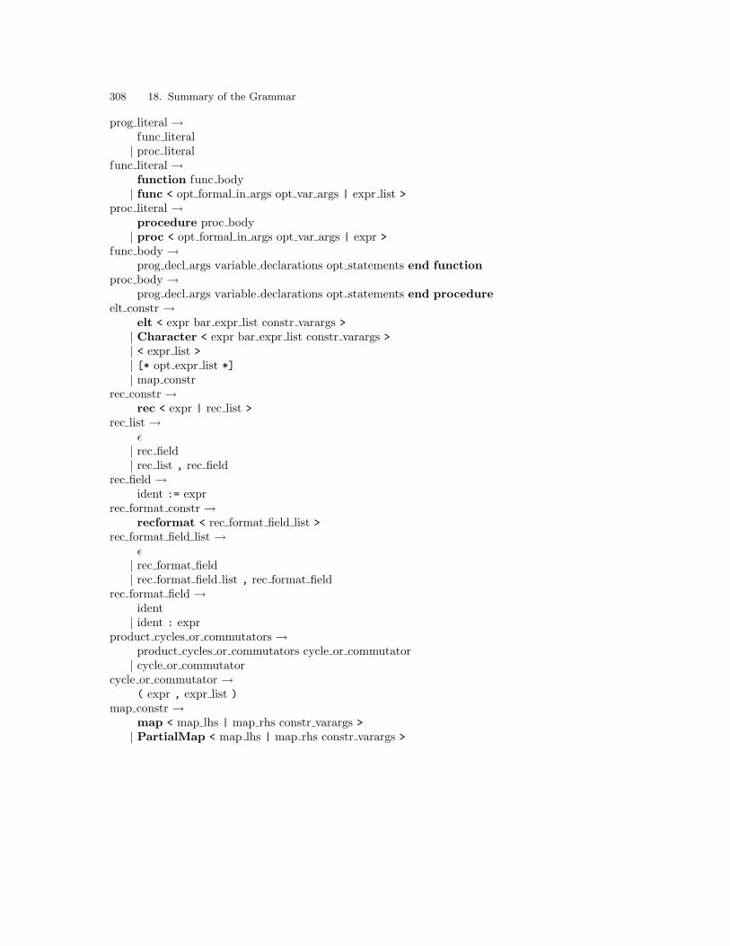
308 18. Summary of the Grammar
prog literal →func literal| proc literal
func literal →function func body| func < opt formal in args opt var args | expr list >
proc literal →procedure proc body| proc < opt formal in args opt var args | expr >
func body →prog decl args variable declarations opt statements end function
proc body →prog decl args variable declarations opt statements end procedure
elt constr →elt < expr bar expr list constr varargs >| Character < expr bar expr list constr varargs >| < expr list >| [* opt expr list *]| map constr
rec constr →rec < expr | rec list >
rec list →ε| rec field| rec list , rec field
rec field →ident := expr
rec format constr →recformat < rec format field list >
rec format field list →ε| rec format field| rec format field list , rec format field
rec format field →ident| ident : expr
product cycles or commutators →product cycles or commutators cycle or commutator| cycle or commutator
cycle or commutator →( expr , expr list )
map constr →map < map lhs | map rhs constr varargs >| PartialMap < map lhs | map rhs constr varargs >
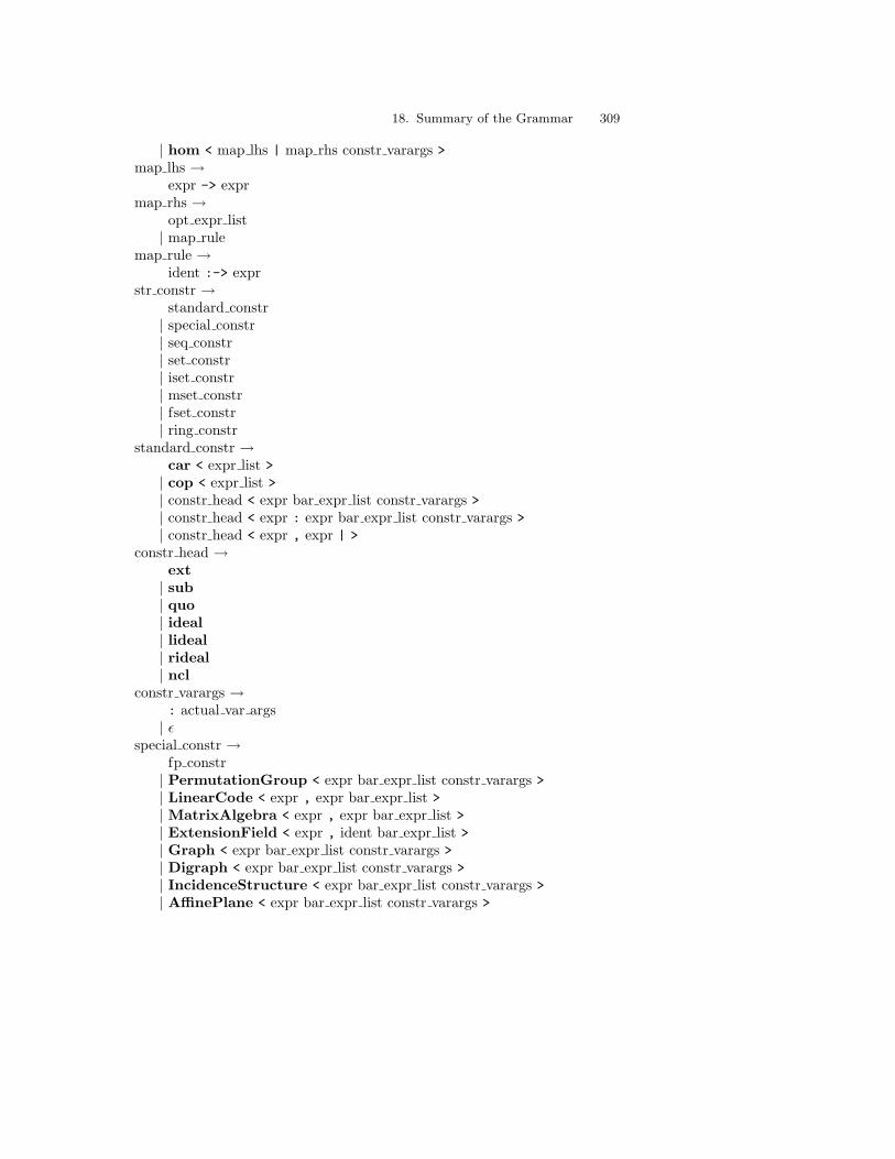
18. Summary of the Grammar 309
| hom < map lhs | map rhs constr varargs >map lhs →
expr -> exprmap rhs →
opt expr list| map rule
map rule →ident :-> expr
str constr →standard constr| special constr| seq constr| set constr| iset constr| mset constr| fset constr| ring constr
standard constr →car < expr list >| cop < expr list >| constr head < expr bar expr list constr varargs >| constr head < expr : expr bar expr list constr varargs >| constr head < expr , expr | >
constr head →ext| sub| quo| ideal| lideal| rideal| ncl
constr varargs →: actual var args| ε
special constr →fp constr| PermutationGroup < expr bar expr list constr varargs >| LinearCode < expr , expr bar expr list >| MatrixAlgebra < expr , expr bar expr list >| ExtensionField < expr , ident bar expr list >| Graph < expr bar expr list constr varargs >| Digraph < expr bar expr list constr varargs >| IncidenceStructure < expr bar expr list constr varargs >| AffinePlane < expr bar expr list constr varargs >

310 18. Summary of the Grammar
| ProjectivePlane < expr bar expr list constr varargs >| NearLinearSpace < expr bar expr list constr varargs >| LinearSpace < expr bar expr list constr varargs >| Design < expr , expr bar expr list constr varargs >| MatrixGroup < expr , expr bar expr list constr varargs >
ring constr →ring constr tok < expr bar expr list constr varargs >
ring constr tok →frac| loc| comp
fp constr →fp constr tok < ident list bar opt expr list opt varargs >
fp constr tok →Group| Semigroup| Monoid| Algebra| PolycyclicGroup| AbelianGroup
set constr → range | expr | range | opt expr list | expr | opt expr list | expr : designator list rl setq pred | expr | expr : designator list rl setq pred
seq constr →[ range ]| [ expr | range ]| seq constr list| [ expr | opt expr list ]| [ expr : designator list rl setq pred ]| [ expr | expr : designator list rl setq pred ]
seq constr list →[ ]| [ seq list ]
seq list →expr| seq list , expr
iset constr →@ opt expr list @| @ expr | opt expr list @| @ expr : designator list rl setq pred @

18. Summary of the Grammar 311
| @ expr | expr : designator list rl setq pred @mset constr →
* opt expr list *| * expr | opt expr list *| * expr : designator list rl setq pred *| * expr | expr : designator list rl setq pred *
fset constr →! ident in expr setq pred !
setq pred →ε| | expr
designator list lr →designator list lr , designator| designator
designator list rl →designator list rl , designator| designator
designator →ident list in expr
bar expr list →| opt expr list
bar opt expr list opt varargs →| opt expr list constr varargs
pred constr →exists pred result expr : designator list rl setq pred | forall pred result expr : designator list rl setq pred | random expr : designator list rl setq pred | rep expr : designator list rl setq pred
pred result →ε| ( expr list )
prog decl args →( formal in args formal prog in args end| ( formal prog in args end
formal prog in args end →)| : actual var args )
formal in args →formal in args , formal in arg| formal in arg
formal in arg →ident| ~ ident
opt formal in args →

312 18. Summary of the Grammar
ε| formal in args
actual func args →( expr list actual func in args end| ( actual func in args end
actual func in args end →)| : actual var args )
actual var arg →ident := expr| ident
opt var args →ε| : actual var args
actual var args →actual var args , actual var arg| actual var arg
ident →Identifier
ident list →ident list , ident| ident
ident underscore list →ident underscore list , ident underscore| ident underscore
ident underscore →ident| _
variable declarations →ε| variable declarations local ident list ;
intrinsic →intrinsic ident ( intrinsic args actual func in args end intrinsic opt
intrinsic return types intrinsic comment variable declarationsopt statements end intrinsic
intrinsic args →ε| intrinsic args list
intrinsic args list →intrinsic arg| intrinsic args list , intrinsic arg
intrinsic arg →ident| ident :: intrinsic type
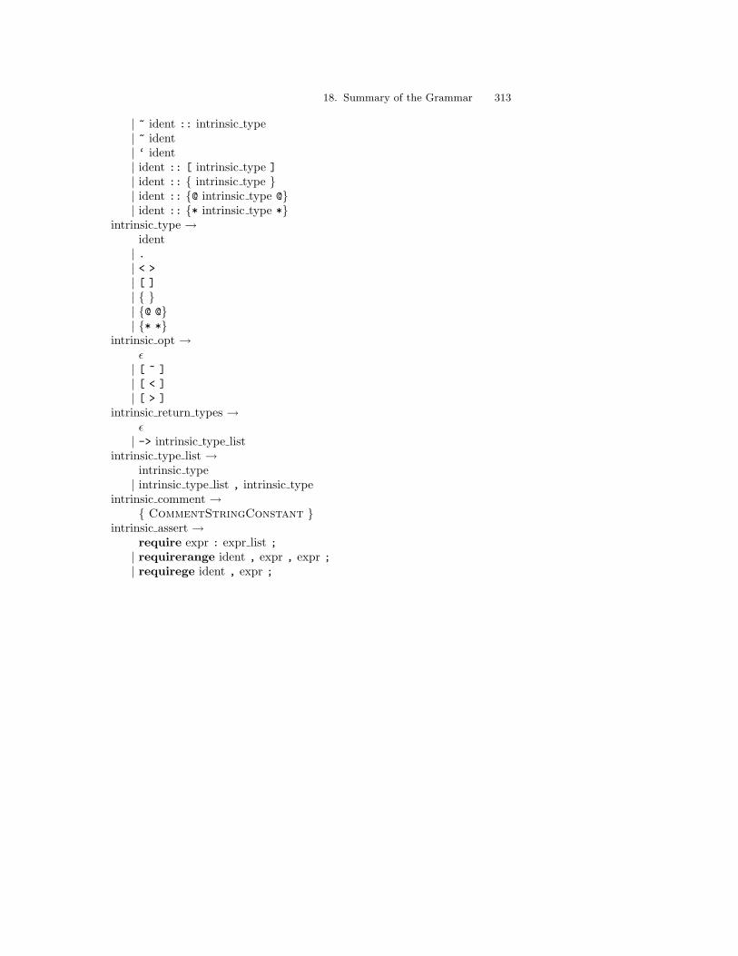
18. Summary of the Grammar 313
| ~ ident :: intrinsic type| ~ ident| ‘ ident| ident :: [ intrinsic type ]| ident :: intrinsic type | ident :: @ intrinsic type @| ident :: * intrinsic type *
intrinsic type →ident| .| < >| [ ]| | @ @| * *
intrinsic opt →ε| [ ~ ]| [ < ]| [ > ]
intrinsic return types →ε| -> intrinsic type list
intrinsic type list →intrinsic type| intrinsic type list , intrinsic type
intrinsic comment → CommentStringConstant
intrinsic assert →require expr : expr list ;| requirerange ident , expr , expr ;| requirege ident , expr ;


Part V
Rings and Fields


19. Overview of Rings and Fields
This chapter consists of an overview of the main categories of commutativerings in Magma, and the operations that may be performed on them. Fieldsare included in the discussion, as special cases of rings.
The various categories of commutative rings cover a very wide spectrum,and some of the most important objects in computer algebra are found here.Subsequent chapters explain in detail how to use the most important par-ticular types of commutative rings, such as the ring of integers ZZ, the fieldof rational numbers Q, residue class rings ZZ/mZZ (see Chapter 20), real andcomplex fields (see Chapter ??), univariate and multivariate polynomial rings(see Chapter 21 and Chapter 22), power and Laurent series rings (see Chapter??), finite fields (see Chapter ??), number fields (see Chapter 25), functionfields (see Chapter ??), p-adic and local rings and fields (Chapter ??). Someimportant types of non-commutative rings (such as matrix rings) appear inthe part on algebras. Their category names (like AlgMat) start with Alg,whereas the names of ring categories usually start with Rng, or with Fld ifonly fields are involved.
In this Chapter we describe some of the general principles for the construc-tion and use of rings and fields, and some principles underlying the designand organization of this diverse area.
19.1 Creating Rings and Fields
Two different families of ring creation functions can be distinguished. Thefirst family is that of standard functions to create rings (and fields) directly.The second family consists of constructors and functions that create newrings from existing ones.
19.1.1 Standard creation functions
Many rings and fields in Magma may be created directly using standardfunctions. Thus ZZ, Q, IR, C, finite fields GFq and residue class rings ZZ/mZZ

318 19. Overview of Rings and Fields
may be created using an intrinsic function with the appropriate arguments.Here are some examples:
> Q := RationalField();> Q;Rational Field
> Z12 := ResidueClassRing(12);> Z12;Residue class ring of integers modulo 12
> G := FiniteField(5, 2);> G;Finite field of size 5^2
> Category(Q), Category(Z12), Category(G);FldRat RngIntRes FldFin
The meaning of the arguments in the above will be clear. In certain cases,such as the finite field example, different numbers of arguments are allowed:FiniteField(25) is synonymous to FiniteField(5, 2).
Table 19.1. Functions for standard rings
IntegerRing PolynomialRing FiniteField
RationalField PowerSeriesRing FunctionField
RealField LaurentSeriesRing NumberField
ComplexField pAdicRing pAdicField
Arguments are not always just integer parameters; here is the constructionof the number field Q( 3
√2).
R<x> := PolynomialRing(Integers());K<k> := NumberField(x^3-2);
We will comment on the use of angle brackets further on.
As we saw already, in cases like the definition of the ring of integers andthe rational field, sometimes no argument is needed at all; this is also truefor the construction of the real (and complex) fields. The rings ZZ, Q, and IRhave another feature in common: they are already present when Magma isstarted up. This makes it possible to define integers, rational numbers andreal numbers without having to create their parents first.
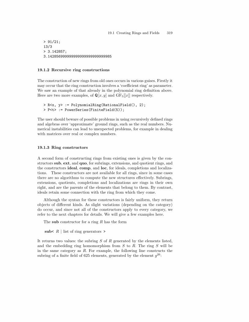
19.1 Creating Rings and Fields 319
> 91/21;13/3> 3.142857;3.142856999999999999999999999985
19.1.2 Recursive ring constructions
The construction of new rings from old ones occurs in various guises. Firstly itmay occur that the ring construction involves a ‘coefficient ring’ as parameter.We saw an example of that already in the polynomial ring definition above.Here are two more examples, of Q[x, y] and GF5[[x]] respectively.
> R<x, y> := PolynomialRing(RationalField(), 2);> P<t> := PowerSeries(FiniteField(5));
The user should beware of possible problems in using recursively defined ringsand algebras over ‘approximate’ ground rings, such as the real numbers. Nu-merical instabilities can lead to unexpected problems, for example in dealingwith matrices over real or complex numbers.
19.1.3 Ring constructors
A second form of constructing rings from existing ones is given by the con-structors sub, ext, and quo, for subrings, extensions, and quotient rings, andthe constructors ideal, comp, and loc, for ideals, completions and localiza-tions. These constructors are not available for all rings, since in some casesthere are no algorithms to compute the new structures effectively. Subrings,extensions, quotients, completions and localizations are rings in their ownright, and are the parents of the elements that belong to them. By contrast,ideals retain some connection with the ring from which they come.
Although the syntax for these constructors is fairly uniform, they returnobjects of different kinds. As slight variations (depending on the category)do occur, and since not all of the constructors apply to every category, werefer to the next chapters for details. We will give a few examples here.
The sub constructor for a ring R has the form
sub< R | list of ring generators >
It returns two values: the subring S of R generated by the elements listed,and the embedding ring homomorphism from S to R. The ring S will bein the same category as R. For example, the following line constructs thesubring of a finite field of 625 elements, generated by the element g26:

320 19. Overview of Rings and Fields
> G<g> := FiniteField(625);> F<f>, m := sub< G | g^26 >;> m(f^2);g^52
The syntax of the ideal constructor is similar to that of the sub constructor.For some categories of rings the ideals form a separate category in Magma.
Here is an ideal in a univariate polynomial ring:
> R<x> := PolynomialRing(RationalField());> f := x^3 + 1/2*x^2 - 3*x - 3/2;> I := ideal< R | f >;> I;Ideal of Univariate Polynomial Algebra in xover Rational Field generated by x^3 + 1/2*x^2 - 3*x - 3/2
The quo constructor creates the quotient of a ring R by an ideal of R. Itreturns two values: the quotient, and the natural homomorphism from thering to the quotient. Continuing the previous example,
> Q<y>, h := quo< R | I >;> Q, h;Univariate Quotient Polynomial Algebra in yover Rational Field with modulus y^3 + 1/2*y^2 - 3*y - 3/2Mapping from: RngUPol: R to RngUPolRes: Q> h(x), h(f);y0
The ideal may be specified explicitly as an ideal, as above, or in terms of itsgenerators:
> Q2<z> := quo< R | f >;> Q2;Univariate Quotient Polynomial Algebra in zover Rational Field with modulus z^3 + 1/2*z^2 - 3*z - 3/2
The quotient is generally an object of another category than that of the ring;which category depends on R.
The ext constructor has a limited applicability in categories of fields andfor transcendental extensions: it may be used to extend finite fields or numberfields, and to create polynomial rings.
For transcendental extensions there are two versions:

19.1 Creating Rings and Fields 321
ext< R | >
is the same as PolynomialRing(R), returning a univariate polynomial ringover R, and:
ext< R, n | >
is the same as PolynomialRing(R,n), returning a multivariate polynomialring of rank n over R.
> P<q,r,s,t> := ext< Z, 7 | >;> P;Polynomial ring of rank 7 over Integer RingLexicographical OrderVariables: q, r, s, t, $.5, $.6, $.7
The main constructor for algebraic extensions has the form
ext< F | f >
where f is a monic irreducible polynomial over F . The constructor returnsan extension E of F by a root of f . For example:
> K<w> := GF(8);> PK<X> := PolynomialRing(K);> f := X^2 + w*X + 1;> IsIrreducible(f);true> E<alpha> := ext< K | f >;> E;Finite field of size 2^6> IsZero(Evaluate(f, alpha));true
The completion constructor
comp< F | list of ideal generators >
is equivalent to Completion(F, I) Both return the completion of F at I, ifI is the zero ideal or a prime ideal of a the ring of integers R of a field F , aswell as a mapping from F to C.
As the examples indicate, there are also intrinsic Magma functions toconstruct certain kinds of completions (Laurent series rings and p-adic fields):

322 19. Overview of Rings and Fields
> Q := RationalField();> F := FunctionField(Q);> comp< F | 0 > eq LaurentSeriesRing(Q);true
> Z := IntegerRing();> comp< Q | 3 > eq pAdicField(3);true
If R is a ring and P is a prime ideal of R, the localization of R at P may becreated with the function Localization(R, P ) or the constructor
loc< R | list of ideal generators >
The function and constructor each return the localization L and a mappingfrom R to L.
For example, the localization of ZZ at 5 is the valuation ring of Q5 (whichmay also be created using the function ValuationRing):
> locn, m := loc< Z | 5 >;> locn, m;Valuation ring of Rational FieldMapping from: RngInt: Z to RngVal: locn> ValuationRing(RationalField(), 5);Valuation ring of Rational Field
19.1.4 Other associated ring constructions
There are more ways of creating new rings out of existing ones; usually theseare category-specific. Some are merely access functions (like CoefficientRing,PrimeField, or GroundField), others construct entirely new objects. Wemention two important field constructions: that of fields of fractions, and thatof residue class fields.
The set of all elements of the form a/b, where a and b are elements of anintegral domain D with b 6= 0, forms the field of fractions of D, when twosuch elements a1/b1 and a2/b2 are considered equal when a1 · b2 = a2 · b1.The Magma function which creates this field is FieldOfFractions(D). Itis available for several categories of domain. Conversely, IntegerRing(K)returns the ring of integers of a field K.
The simplest example of this kind of field is the rational field, which isthe field of fractions of the integer ring:
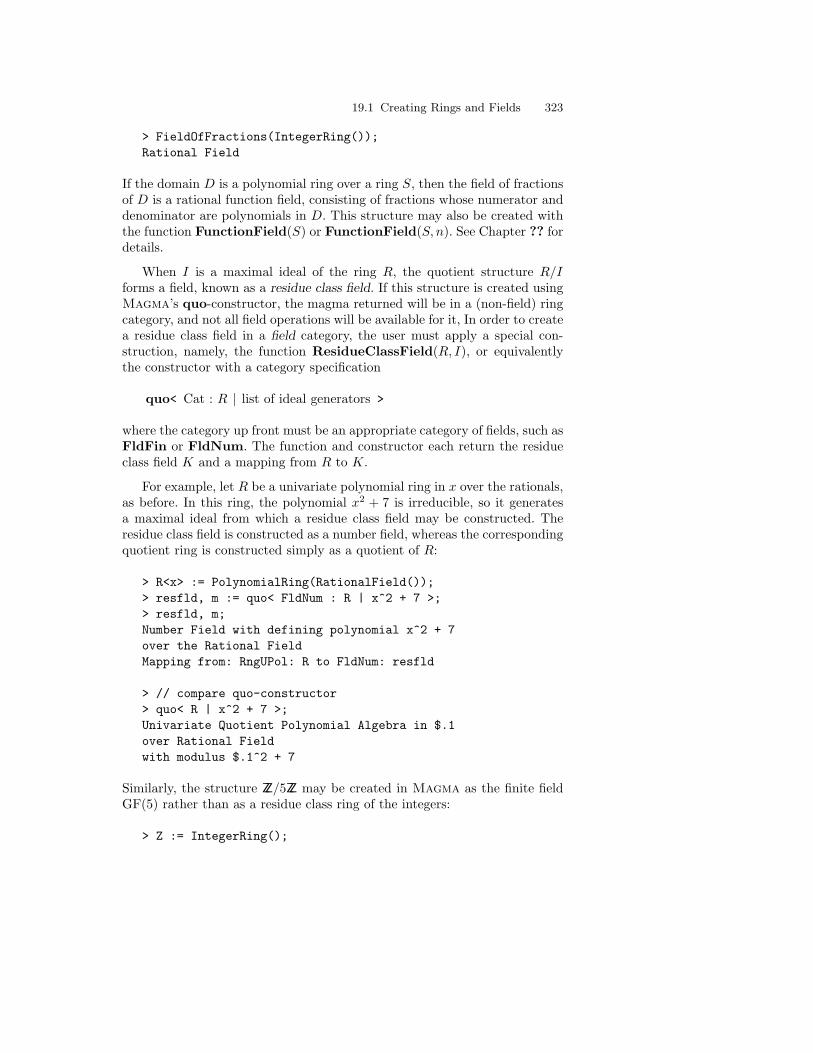
19.1 Creating Rings and Fields 323
> FieldOfFractions(IntegerRing());Rational Field
If the domain D is a polynomial ring over a ring S, then the field of fractionsof D is a rational function field, consisting of fractions whose numerator anddenominator are polynomials in D. This structure may also be created withthe function FunctionField(S) or FunctionField(S, n). See Chapter ?? fordetails.
When I is a maximal ideal of the ring R, the quotient structure R/Iforms a field, known as a residue class field. If this structure is created usingMagma’s quo-constructor, the magma returned will be in a (non-field) ringcategory, and not all field operations will be available for it, In order to createa residue class field in a field category, the user must apply a special con-struction, namely, the function ResidueClassField(R, I), or equivalentlythe constructor with a category specification
quo< Cat : R | list of ideal generators >
where the category up front must be an appropriate category of fields, such asFldFin or FldNum. The function and constructor each return the residueclass field K and a mapping from R to K.
For example, let R be a univariate polynomial ring in x over the rationals,as before. In this ring, the polynomial x2 + 7 is irreducible, so it generatesa maximal ideal from which a residue class field may be constructed. Theresidue class field is constructed as a number field, whereas the correspondingquotient ring is constructed simply as a quotient of R:
> R<x> := PolynomialRing(RationalField());> resfld, m := quo< FldNum : R | x^2 + 7 >;> resfld, m;Number Field with defining polynomial x^2 + 7over the Rational FieldMapping from: RngUPol: R to FldNum: resfld
> // compare quo-constructor> quo< R | x^2 + 7 >;Univariate Quotient Polynomial Algebra in $.1over Rational Fieldwith modulus $.1^2 + 7
Similarly, the structure ZZ/5ZZ may be created in Magma as the finite fieldGF(5) rather than as a residue class ring of the integers:
> Z := IntegerRing();

324 19. Overview of Rings and Fields
> I5 := ideal< Z | 5 >;> I5;Ideal of Integer Ring generated by 5> ResidueClassField(Z, I5);Finite field of size 5Mapping from: RngInt: Z to GF(5)> quo< Z | I5 >;Residue class ring of integers modulo 5
Finally, if the initial ring is a polynomial ring over a finite field then anextension of this field may be produced:
> Rgf7<y> := PolynomialRing(GF(7));> quo< FldFin : Rgf7 | y^5 + 3*y + 1 >;Finite field of size 7^5Mapping from: RngUPol: Rgf7 to GF(7^5)
19.2 Operations on Ring Elements
Methods for creating elements of a ring R depend on the category of R, but itgenerally involves one of the following constructions: the coercion into R of anelement or a sequence of elements of a ring related to R; an expression in thegenerators of the ring, using the arithmetic operations shown in Table 19.3(p. 327); or the construction of some special element of R.
> Z12 := Integers(12);> Z12 ! 57;9
> R<x> := PolynomialRing(RationalField());> p := R ! [5/4, 0, 13/7, -1, 2]; p;2*x^4 - x^3 + 13/7*x^2 + 5/4
> R<s, t> := PolynomialRing(FiniteField(5), 2);> s*t^5 + 4*t + 7;s*t^5 + 4*t + 7
We will briefly discuss the use of the angle brackets on the left handside of an assignment here; see also Chapter 21. Angle brackets are used togive names to ‘indeterminates’ (as in the above example), or elements thatare ‘generators’ in a more general sense, for example in number fields orfinite fields. (‘Generator’ here means generator of the new ring that is being

19.2 Operations on Ring Elements 325
Table 19.2. Ring element creation
Magma Meaning
R.i i-th generator of ring R
Zero(R) Additive identity of ring R
One(R) Multiplicative identity of unitary ring R
Representative(R),Rep(R) A representative element of ring R
Random(R) A random element of finite ring R
Parent(x) Parent ring of ring element x
Category(x),Type(x) Category to which ring element x belongs
constructed as an algebra over the ring it is defined over.) It is very importantto know that the effect of:
> R<s, t> := PolynomialRing(FiniteField(5), 2);
instead of
> R := PolynomialRing(FiniteField(5), 2);
is twofold. In the first place the ‘names’ placed between angle brackets (sep-arated by comma’s) are used as strings in Magma output: indeed, elementsof R will be printed as polynomials in which ‘s’ and ‘t’ are the indetermi-nates. Simultaneously, however, (two) identifiers (s and t) will be assignedvalues, being the first indeterminates or generators in the ring that is beingconstructed. This makes it possible from here on to define elements (of R inthe above example) using the identifiers (s and t).
That the two operations are indeed distinct can be seen from the follow-ing example, where s and t as identifiers are reassigned, but the output ofpolynomials is not affected:
> R<s, t> := PolynomialRing(FiniteField(5), 2);> f := s^3+t^2;> f;s^3 + t^2> s := -2; t := 1;> s^3 + t^2;-7> f;s^3 + t^2
If identifiers have been reassigned, or if the angle brackets were not used inthe first place, it is still possible to do the assignment afterwards. For this the
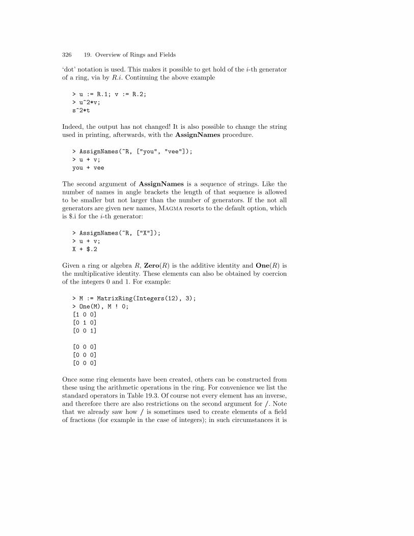
326 19. Overview of Rings and Fields
‘dot’ notation is used. This makes it possible to get hold of the i-th generatorof a ring, via by R.i. Continuing the above example
> u := R.1; v := R.2;> u^2*v;s^2*t
Indeed, the output has not changed! It is also possible to change the stringused in printing, afterwards, with the AssignNames procedure.
> AssignNames(~R, ["you", "vee"]);> u + v;you + vee
The second argument of AssignNames is a sequence of strings. Like thenumber of names in angle brackets the length of that sequence is allowedto be smaller but not larger than the number of generators. If the not allgenerators are given new names, Magma resorts to the default option, whichis $.i for the i-th generator:
> AssignNames(~R, ["X"]);> u + v;X + $.2
Given a ring or algebra R, Zero(R) is the additive identity and One(R) isthe multiplicative identity. These elements can also be obtained by coercionof the integers 0 and 1. For example:
> M := MatrixRing(Integers(12), 3);> One(M), M ! 0;[1 0 0][0 1 0][0 0 1]
[0 0 0][0 0 0][0 0 0]
Once some ring elements have been created, others can be constructed fromthese using the arithmetic operations in the ring. For convenience we list thestandard operators in Table 19.3. Of course not every element has an inverse,and therefore there are also restrictions on the second argument for /. Notethat we already saw how / is sometimes used to create elements of a fieldof fractions (for example in the case of integers); in such circumstances it is

19.3 Testing Properties of a Ring 327
useful also to have exact division, where the result is in the ring itself. Theoperator div is provided for that:
> q := 6/3;> q, Parent(q);2 Rational Field> z := 6 div 3;> z, Parent(z);2 Integer Ring
Table 19.3. Ring element arithmetic
Magma Meaning
x + y Sum of elements x and y
−x Additive inverse of x
x− y Difference of elements x and y
n*x x added to itself |n| times, multiplied by thesign of n
x ∗ y Product of elements x and y
x^−1 Multiplicative inverse of unit x
x^n xn, where n is an integer (n may be negativeonly if x is a unit)
x/y xy−1, where y is a unit
There are many Boolean operators and functions for ring elements. Firstly,there are the standard equality-testing operators, eq and ne. Next, there arethe order operators such as gt. They are only available for rings which havea total ordering defined on their elements (see Section 19.4.2); these ringsare the integer ring, the rational field and the real field. The other Booleanoperations on ring elements are the functions beginning with Is, as listed inTable 19.4. For instance:
> a := Integers(12) ! 4;> IsZeroDivisor(a);true> IsZero(3*a); // checktrue

328 19. Overview of Rings and Fields
Table 19.4. Tests on elements of rings
Magma Meaning
IsZero(x) true if x is the additive identity of its parent ring
IsOne(x) true if x is the multiplicative identity of its parent ring
IsMinusOne(x) true if x is the −1 of its parent ring
IsUnit(x) true if xy = 1 for some y in the parent ring
IsNilpotent(x) true if xq = 0 for some q ∈ ZZ+; if true, also returnsthe smallest such q (the index of nilpotence)
IsZeroDivisor(x) true if x 6= 0 and xy = 0 for some y 6= 0
IsRegular(x) true if x is not a zero divisor
IsIdempotent(x) true if x2 = x
IsIrreducible(x) true if x (in an integral domain) is not a unit, and ifwhenever x = ab, then a or b is a unit
IsPrime(x) true if x (in an integral domain) is not 0 nor a unit, andif whenever x|ab, then x|a or x|b
19.3 Testing Properties of a Ring
There are many Boolean functions which test properties of a ring (or field) R.Table 19.5 (p. 329) lists them. The return value depends on the mathematicalproperties of R, not the category to which R belongs. For instance:
> Z9 := ResidueClassRing(9);> IsField(Z9);false> Z7 := ResidueClassRing(7);> IsField(Z7);true> IsPrincipalIdealDomain(Z7);true
This illustrates that if R is known to satisfy the given property then theresult is true, even if a stronger property also holds. If there is no appropriatealgorithm (implemented) for determining the answer, Magma will give anerror message.
Even if a ring R returns true to one of these Boolean functions, operationsemploying this property may not be available if the property does not hold forall rings in the category of R. This follows from the Magma-wide principlethat the operations that apply to an object are given by the category ofdefinition, as explained on p. 47. For instance, Z7 is not a member of a fieldcategory, so it is not possible to construct a vector space over it, even thoughMagma can tell that 27 satisfies the axioms of a field. However, it is possible

19.3 Testing Properties of a Ring 329
Table 19.5. Some tests on properties of a ring
Magma Meaning
IsField(R) true if R is a commutative divisionring
IsOrdered(R) true if ‘greater than’ is defined in R
IsEuclideanDomain(R) true if R is a domain and has aknown Euclidean norm function
IsEuclideanRing(R) true if R has a known Euclideannorm function
IsPrincipalIdealDomain(R),IsPID(R)
true if R is a domain and every idealof R has the form aR for some a ∈ R
IsPrincipalIdealRing(R),IsPIR(R)
true if every ideal of R has the formaR for some a ∈ R
IsUniqueFactorizationDomain(R),IsUFD(R)
true if R is a domain and factoriza-tion is unique
IsIntegralDomain(R),IsDomain(R)
true if R is commutative, has a 1 6=0, and has no zero divisors
IsCommutative(R) true if R is commutative
IsDivisionRing(R) true if R has a 1 6= 0, and everya ∈ R except 0 has an inverse
IsUnitary(R) true if R has a 1
IsFinite(R) true if R has a finite number of ele-ments; if true, also returns the car-dinality #R of R
to construct a vector space over FiniteField(7), which is isomorphic to Z7 .The user must explicitly create the structure as a field if Magma is expectedto regard it as a field.
An important ring property is whether it is unitary, that is, whether ithas a multiplicative identity. This is tested by IsUnitary(R). Many Magmaoperations involving rings are only permitted if the ring is unitary. There isa certain subtlety involved here: a subring is regarded as unitary by Magmaonly if it contains the multiplicative identity of its generic ring. For example,in the ideal I of ZZ/12ZZ generated by 5, the element 25 is a multiplicativeidentity, but since I does not contain the one of ZZ/12ZZ, it is not regarded asunitary:
> I := ideal< ResidueClassRing(30) | 5 >;> I;Ideal of residue class ring of integers modulo 30generated by 5> forall a : a in I | 25*a eq a ;true> IsUnitary(I);
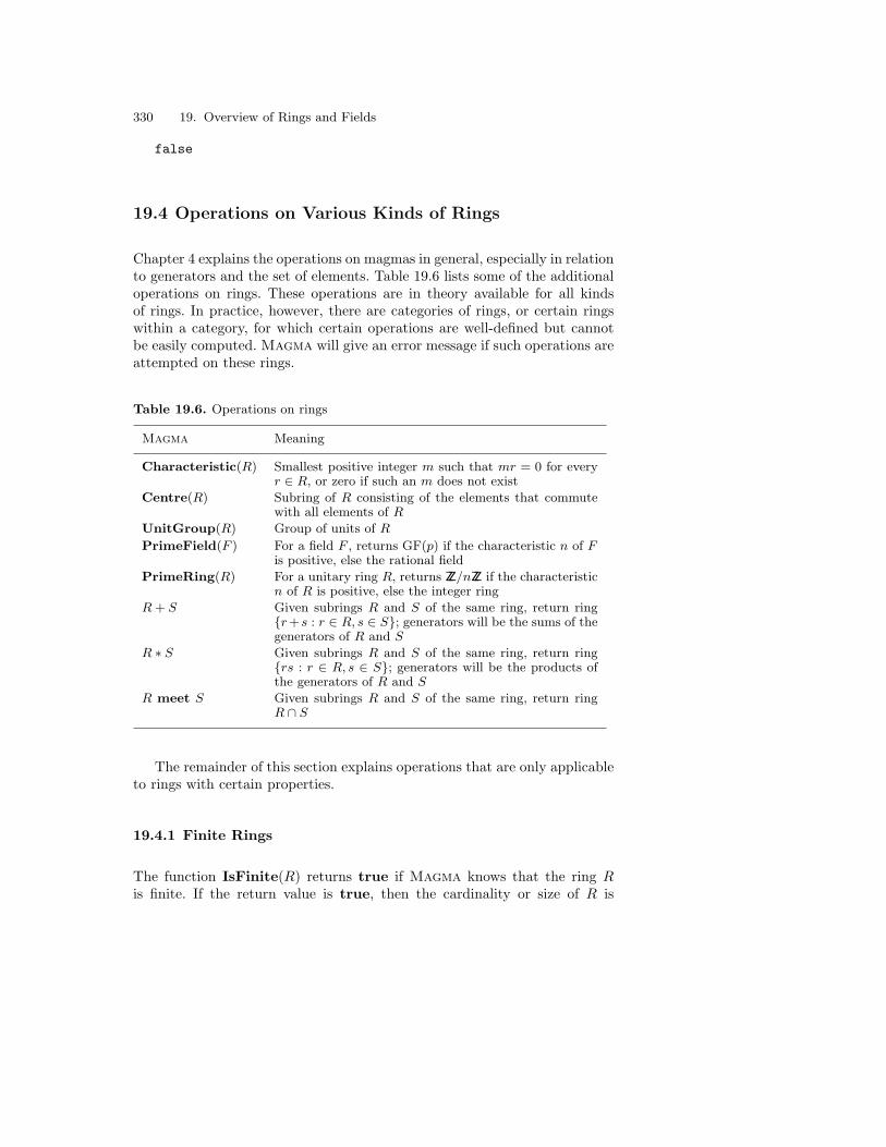
330 19. Overview of Rings and Fields
false
19.4 Operations on Various Kinds of Rings
Chapter 4 explains the operations on magmas in general, especially in relationto generators and the set of elements. Table 19.6 lists some of the additionaloperations on rings. These operations are in theory available for all kindsof rings. In practice, however, there are categories of rings, or certain ringswithin a category, for which certain operations are well-defined but cannotbe easily computed. Magma will give an error message if such operations areattempted on these rings.
Table 19.6. Operations on rings
Magma Meaning
Characteristic(R) Smallest positive integer m such that mr = 0 for everyr ∈ R, or zero if such an m does not exist
Centre(R) Subring of R consisting of the elements that commutewith all elements of R
UnitGroup(R) Group of units of R
PrimeField(F ) For a field F , returns GF(p) if the characteristic n of Fis positive, else the rational field
PrimeRing(R) For a unitary ring R, returns ZZ/nZZ if the characteristicn of R is positive, else the integer ring
R + S Given subrings R and S of the same ring, return ringr+s : r ∈ R, s ∈ S; generators will be the sums of thegenerators of R and S
R ∗ S Given subrings R and S of the same ring, return ringrs : r ∈ R, s ∈ S; generators will be the products ofthe generators of R and S
R meet S Given subrings R and S of the same ring, return ringR ∩ S
The remainder of this section explains operations that are only applicableto rings with certain properties.
19.4.1 Finite Rings
The function IsFinite(R) returns true if Magma knows that the ring Ris finite. If the return value is true, then the cardinality or size of R is

19.4 Operations on Various Kinds of Rings 331
also returned. The cardinality of R may also be obtained directly from theexpression #R.
If Magma knows that R is finite then it can usually calculate the elementsof R. If so, then the set of these elements is Set(R). It will also be possible toiterate over R, that is, to type x in R within a set/sequence constructoror at the top of a for-loop.
19.4.2 Ordered Rings
Table 19.7. Operations for elements of totally ordered rings
Magma Meaning
x lt y true if x < y
x le y true if x ≤ y
x gt y true if x > y
x ge y true if x ≥ y
Maximum(x, y),Max(x, y) The larger of the elements x and y
Maximum(Q),Max(Q) Returns (i) the largest of the elements in thesequence Q (ii) the position of this element
Minimum(x, y),Min(x, y) The smaller of the elements x and y
Minimum(Q),Min(Q) Returns (i) the largest of the elements in thesequence Q (ii) the position of this element
Table 19.7 lists the operations for elements of a totally ordered ring R,that is, a ring for which IsOrdered(R) returns true. If a ring does not havea total ordering defined on its elements then it makes no sense to comparethe elements for size. The integer ring, rational field and real field are alltotally ordered.
19.4.3 Euclidean Rings
A Euclidean ring R is a ring which has a known Euclidean norm function,that is, a function φ from the set S of regular elements of R to the non-negative integers such that (a) x|y implies φ(x) ≤ φ(y) and (b) if x ∈ Rand y ∈ S then there exist q, r ∈ R such that x = yq + r and either r = 0or φ(r) < φ(y). Important examples of Euclidean rings are the integers, inwhich φ is the absolute value, and the univariate polynomials over a field, inwhich φ is the degree of the polynomial.

332 19. Overview of Rings and Fields
The function IsEuclideanRing(R) returns true if R is known to have aEuclidean norm. Most commonly-investigated Euclidean rings are also inte-gral domains; this is tested by IsEuclideanDomain(R). Given an elementx of a Euclidean ring R, EuclideanNorm(x) returns φ(x). It is not practicalfor Magma to attempt to find a Euclidean norm for any given ring, so itsknowledge of whether a norm exists is rather restricted, and it always usesthe standard mathematical choice for φ as the norm.
The purpose of a Euclidean norm is to allow division-with-remainder totake place in the ring. In the situation described above, with the equationx = yq+r, the expression x div y returns the quotient q, and x mod yreturns the remainder r. The function Quotrem(x, y) returns both q and r,in that order.
19.4.4 Unique Factorization Domains
Table 19.8. Operations on elements of unique factorization domains
Magma Meaning
GCD(x, y) Greatest common divisor of x and y
GCD(Q) Greatest common divisor of terms in sequence Q
LCM(x, y) Least common multiple of x and y
LCM(Q) Least common multiple of terms in sequence Q
XGCD(x, y) Extended gcd: returns ring elements g, p, q such that g isgcd of x and y and g = px + qy
XGCD(Q) Given Q = [x1, . . . xr], returns gcd g of Q and sequenceM = [m1, . . . , mr] such that g =
Pri=1 mixi
IsDivisible(x, y) true if x is divisible by y
IsAssociate(x, y) true if x = uy for some unit u
Factorization(x) Returns (i) sequence [< f1, k1 >, . . . , < fr, kr >] where thefi are irreducible and the ki are non-negative integers, and(ii) unit u, such that x = ufk1
1 · · · fkrr
A unique factorization domain (UFD) is a domain R such that every non-zero element factorizes uniquely (up to order and associates) into a productof irreducibles. IsUFD(R) returns true if R is known by Magma to be aUFD. Table 19.8 (p. 332) shows the operations for UFDs.
In the integer ring and in polynomial rings over the integer ring or a field,which are the major examples of UFDs, factorization of a ring element x isan important and non-trivial task. The function Factorization(x) returnsthe factorization of x in the form of a factorization sequence and a unit. Forinstance:

19.4 Operations on Various Kinds of Rings 333
> a, b := Factorization(-3798386541);> a, b;[ <3, 4>, <181, 1>, <509, 2> ]-1
The output indicates that −3798386541 = −1 · 34 · 1811 · 5092.
Several algorithms have been developed to perform factorization, andMagma supports a number of these algorithms, for each of integer factoriza-tion and polynomial factorization. To specify the desired method, the usershould employ the function Factorization(x) with one or more parameters;see Section 20.4.2 for an explanation of their use. For instance, if f is apolynomial then the function Factorization(f) has a parameter Al, whichcan take any of three string values. The following lines demonstrate how tofactorize a polynomial using the "BerlekampSmall" algorithm:
> GF503polys<r> := PolynomialAlgebra(GF(503));> a, b:=Factorization(3*r^250+500: Al := "BerlekampSmall");> a;[
<r + 1, 1>,<r + 502, 1>,<r^4 + r^3 + r^2 + r + 1, 1>,<r^4 + 502*r^3 + r^2 + 502*r + 1, 1>,<r^20 + r^15 + r^10 + r^5 + 1, 1>,<r^20 + 502*r^15 + r^10 + 502*r^5 + 1, 1>,<r^100 + r^75 + r^50 + r^25 + 1, 1>,<r^100 + 502*r^75 + r^50 + 502*r^25 + 1, 1>
]> b;3
For more information, see Section 21.6. In the case of integer factorization, thefunction Factorization(n) uses a combination of algorithms, but the param-eters may be set to specify the extent to which each algorithm is employed,and the details of its use. For instance, the following call to the function al-ters the default values of the number of curves used in the first elliptic curveattack, and the upper bound for the trial divisors (these changes are notnecessarily for the better!):
> Factorization(112377669312366219120309:> PollardRhoLimit := 100, MPQSLimit := 0);[ <3, 8>, <181, 2>, <509, 4>, <7789, 1> ]
The next chapter describes these parameters, (see p. 356).


20. Ring of Integers and Field of Rationals
Reflecting the fundamental role played by the ring of rational integers inmathematics, Magma contains highly optimized code for performing arith-metic with arbitrary precision integers. This is augmented with advancedtools for factoring integers (elliptic curve and quadratic sieve methods) andfor proving primality (an elliptic curve primality prover).
This chapter describes the many operators and functions that are definedfor the ring of integers ZZ and for the rational field Q. Also included is a dis-cussion of residue class rings ZZ/nZZ and their arithmetic. A number of integerfunctions relating to combinatorics are described elsewhere (see Chapter 35).
20.1 Creating Integers and Rationals
No action is required on the part of the user to create the ring of integersZZ or the field of rational numbers Q, since both are automatically definedwhenever Magma is started. In particular, integers and rationals may becreated without reference to their parent since they are recognized from theirsyntax:
> 42;42> 5/7;5/7
Integers of any length may be defined in this manner. However, it is recom-mended that the line continuation character \ be placed at the end of eachline when the number of digits extends over more than one line. Magma alsouses the backslash to break long lines of output:
> m := 1234567890123456789012345678901234567890\> 1234567890123456789012345678901234567890;> m^2;

336 20. Ring of Integers and Field of Rationals
15241578753238836750495351562566681945008382873376009755\22511812231126352691000121932731260478594250876391537570\49236500533455762536198787501905199875019052100
(Use SetColumns to change the number of characters printed on a singleline.)
A rational number may be created by typing the expression p/q (where pand q evaluate to integers and q does not equal zero). Magma stores rationalnumbers in reduced form, where the numerator and denominator are coprimeand the denominator is positive:
> r := 68/-72;> r;-17/18
The standard constructors also apply to the construction of rationals; theelt-constructor elt< Q | p, q > and the coercion Q ! t, where t is a sequence[p, q] both require expressions evaluating to two integers p, q, and create therational p/q.
Magma draws a distinction between the rational number p1 and the in-
teger p, though automatic coercion makes this distinction transparent to theuser in many cases. If the user creates a rational number r whose denomina-tor (in reduced form) equals 1, the number will be stored as an element ofQ, rather than as an element of ZZ, although it will look like an integer whenprinted. The function IsIntegral(r) returns true for such numbers.
The function IntegerRing(), or Integers(), returns the magma corre-sponding to ZZ for use in situations where reference needs to be made to it.Similarly, RationalField() and Rationals() return the field Q. For exam-ple, when using the function MatrixRing to define a matrix ring over theintegers, ZZ must be given as one of the arguments:
> Z := IntegerRing();> Z;Integer Ring> M := MatrixRing(Z, 5); M;Full Matrix Algebra of degree 5 over Integer Ring
Another common case occurs when applying a strictly integer function to arational argument; for example, the integer 374 is clearly divisible by 2, butomitting the coercion in the example below will lead to a ‘type’ error.
> Factorization( Integers() ! (374/2));[ <11, 1>, <17, 1> ]

20.2 Manipulating Integers and Rationals 337
As will be seen in the next section, this ‘type’ problem would not arise if divwas used rather than / for division.
The category containing the ring of rational integers is RngInt, thatcontaining Q is called FldRat.
20.2 Manipulating Integers and Rationals
20.2.1 Arithmetic
All of the standard arithmetic operations for integers and rationals are avail-able in Magma. The operators denoting addition, subtraction, multiplica-tion, and division are +, −, *, and /. When applied to two members of theFldRatElt category, the result will also be a Magma rational; with the ex-ception of division, which always results in a rational, the binary operationson elements of RngIntElt result in integers again. When one operand is aninteger and the other a rational number the result is always rational.
Addition, subtraction, multiplication, and division may be performed onarbitrarily large integers, the size being restricted only by the amount ofcomputer memory available. For example, the following computation returnsthe exact value of the result, with no approximation or rounding:
> n := 123456789012345678901234567890;> n*(n-1/7);15241578753238836750495351562518562103357284388603414113830
The last result, although integral, is an element of Q. The operator / con-structs the rational number a
b , and consequently always returns an elementof the rational field, even if the division is exact. If this occurs, it is of coursepossible to coerce to RngIntElt using !. Alternatively, one could use div,which returns the integral quotient when applied to two integers; togetherwith the mod operator this returns the quotient and remainder pair of thedivision of two integers a and b. Both quotient q and remainder r (in thatorder) are also returned by the single function Quotrem(a, b). The quoitientand remainder are determined by the rules that a = qb + r, and r has thesame sign as b while satisfying 0 ≤ |r| < |b|.
> q, r := Quotrem(123871, 4249);> q, r;29 650> 123871 div 4249;29

338 20. Ring of Integers and Field of Rationals
> 123871 mod 4249;650> 374 div 2;187> Type($1);RngIntElt
As a longer example, consider the problem of writing a positive integer Nin the form N − 1 = 2sd, where s and d are positive integers. The followingfunction EvenexpOdd(N) has s and d as its return values:
To perform this example online, type load "I96c20e1";
> EvenexpOdd := function(N)> s := 0; d := N - 1;> q, r := Quotrem(d, 2);> while r eq 0 do> s +:= 1;> d := q;> q, r := Quotrem(d, 2);> end while;> return s, d;> end function;
For instance:
> N := 158561449985;> EvenexpOdd(N);11 77422583> N - 1 eq 2^11 * 77422583;true
The expression m^k denotes the k-th power mk of m. If the exponent k is arational or real number the result will be a real number but in this chapterk will be assumed to be an integer. Provided that k is a non-negative integerand m is an integer, then the result will be an integer, but in all other cases(m rational or k negative) the result is a rational number. (Note that 0^0 isdefined to be 1, following convention.) The result may be a rational numbereven if it happens to be integral:
> 3^5, Parent(3^5);243 Integer Ring> 3^(-5), Parent(3^(-5));1/243 Rational Field

20.2 Manipulating Integers and Rationals 339
> 1^(-5), Parent(1^(-5));1 Rational Field> (1/2)^-1, Parent((1/2)^-1);2 Rational Field
The exponent k must be a small integer.
Table 20.1. Divisibility functions
Magma Meaning
Quotrem(a, n) Given a and n with n 6= 0, returns (i) quotient q, (ii) re-mainder r, such that a = qn + r and |r| < n (0 < r < n ifn > 0; n < r < 0 if n < 0)
a div n Quotient q when a is divided by n, as in Quotrem
a mod n Remainder r when a is divided by n, as in Quotrem
GCD(a, b) Greatest common divisor of a and b
GCD(Q) Greatest common divisor of the sequence of integers Q
XGCD(a, b) Greatest common divisor d of a and b together with cofac-tors p, q such that d = pa + qb
XGCD(Q) Greatest common divisor of the sequence of integers Q to-gether with cofactors
LCM(a, b) Lowest common multiple of a and b
LCM(Q) Lowest common multiple of the sequence of integers Q
IsDivisible(a, b) true if a is divisible by b; if true, also returns the quotienta/b
IsEven(a) true if and only if integer a is even
IsOdd(a) true if and only if integer a is odd
20.2.2 Elementary Functions
The function GCD computes the greatest common divisor of integers a andb, while LCM returns their least common multiple. The use of GCD isillustrated by looking for a factor of n = 557200336747259. If p is a prime,by Fermat’s Theorem, ap−1 = 1 mod p, for any integer a coprime to p. Thisimplies that p divides am−1, for any multiple m of p−1. So if n has a primedivisor p such that p− 1 divides m, the factor p is easily found:
> n := 67394403;> [ Gcd(2^m-1, n) : m in [2..18] ];[ 3, 1, 3, 31, 9, 1, 3, 73, 93, 1, 9, 1, 3, 31, 3, 1, 1971]> Factorization(n);[ <3, 3>, <31, 1>, <73, 1>, <1103, 1> ]
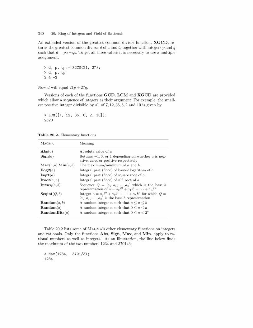
340 20. Ring of Integers and Field of Rationals
An extended version of the greatest common divisor function, XGCD, re-turns the greatest common divisor d of a and b, together with integers p and qsuch that d = pa+ qb. To get all three values it is necessary to use a multipleassignment:
> d, p, q := XGCD(21, 27);> d, p, q;3 4 -3
Now d will equal 21p + 27q.
Versions of each of the functions GCD, LCM and XGCD are providedwhich allow a sequence of integers as their argument. For example, the small-est positive integer divisible by all of 7, 12, 36, 8, 2 and 10 is given by
> LCM([7, 12, 36, 8, 2, 10]);2520
Table 20.2. Elementary functions
Magma Meaning
Abs(a) Absolute value of a
Sign(a) Returns −1, 0, or 1 depending on whether a is neg-ative, zero, or positive respectively
Max(a, b),Min(a, b) The maximum/minimum of a and b
Ilog2(a) Integral part (floor) of base-2 logarithm of a
Isqrt(a) Integral part (floor) of square root of a
Iroot(a, n) Integral part (floor) of nth root of a
Intseq(a, b) Sequence Q = [a0, a1, . . . , an] which is the base brepresentation of a = a0b
0 + a1b1 + · · ·+ anbn
Seqint(Q, b) Integer a = a0b0 + a1b
1 + · · · + anbn for which Q =[a0, a1, . . . , an] is the base b representation
Random(a, b) A random integer n such that a ≤ n ≤ b
Random(a) A random integer n such that 0 ≤ n ≤ a
RandomBits(a) A random integer n such that 0 ≤ n < 2a
Table 20.2 lists some of Magma’s other elementary functions on integersand rationals. Only the functions Abs, Sign, Max, and Min. apply to ra-tional numbers as well as integers. As an illustration, the line below findsthe maximum of the two numbers 1234 and 3701/3:
> Max(1234, 3701/3);1234
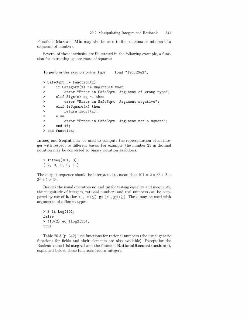
20.2 Manipulating Integers and Rationals 341
Functions Max and Min may also be used to find maxima or minima of asequence of numbers.
Several of these intrinsics are illustrated in the following example, a func-tion for extracting square roots of squares:
To perform this example online, type load "I96c20e2";
> SafeSqrt := function(x)> if Category(x) ne RngIntElt then> error "Error in SafeSqrt: Argument of wrong type";> elif Sign(x) eq -1 then> error "Error in SafeSqrt: Argument negative";> elif IsSquare(x) then> return Isqrt(x);> else> error "Error in SafeSqrt: Argument not a square";> end if;> end function;
Intseq and Seqint may be used to compute the representation of an inte-ger with respect to different bases. For example, the number 25 in decimalnotation may be converted to binary notation as follows:
> Intseq(101, 3);[ 2, 0, 2, 0, 1 ]
The output sequence should be interpreted to mean that 101 = 2× 30 + 2×32 + 1× 34.
Besides the usual operators eq and ne for testing equality and inequality,the magnitude of integers, rational numbers and real numbers can be com-pared by use of lt (for <), le (≤), gt (>), ge (≥). These may be used witharguments of different types:
> 3 lt Log(10);false> (10/2) eq Ilog2(33);true
Table 20.3 (p. 342) lists functions for rational numbers (the usual genericfunctions for fields and their elements are also available). Except for theBoolean-valued IsIntegral and the function RationalReconstruction(s),explained below, these functions return integers.

342 20. Ring of Integers and Field of Rationals
Table 20.3. Operations on rational numbers
Magma Meaning
Numerator(r) Numerator of r (in reduced form)
Denominator(r) Denominator of r (in reduced form)
IsIntegral(r) true if Denominator(r) is one
Abs(r) Absolute value |r| of r
Sign(r) Returns −1, 0, or 1 depending on whether r isnegative, zero, or positive respectively
Floor(r) Greatest integer brc less than or equal to r
Ceiling(r) Smallest integer dre greater than or equal to r
Round(r) Integer nearest r (n + 12
is rounded to n + 1,for n ∈ ZZ)
Truncate(r) Integer part of r, or r rounded towards zero,i.e., Sign(r)*b |r| c
RationalReconstruction(s) Given s in ZZ/mZZ (or GF(m), where m isprime), return true if s has a rational recon-struction r; if true, also return r
When applied to an element s of any residue class ring ZZ/mZZ or any primefinite field, RationalReconstruction(s) returns a Boolean value, with arational number if the Boolean is true. The purpose of this function is toprovide a partial inverse of the function ψm : Q → ZZ/mZZ of taking residuesmodulo m, where the obvious value of ψm is only defined for rational numberswith denominator coprime to m. The value of ψ−1(s) is the rational numberr = p
q (in reduced form) for which ψm(r) = s (i.e., pq−1 ≡ s mod m) and, inaddition, |p|, q ≤
√m/2. Such an r does not always exist, but if it exists it
is unique. For example:
> F := GF(29);> RationalReconstruction(F ! 22);false> RationalReconstruction(F ! 20);true 2/3> F ! (2/3);20
> Z45 := ResidueClassRing(45);> RationalReconstruction(Z45 ! 33);true -3/4> (Z45 ! -3) / 4;33

20.2 Manipulating Integers and Rationals 343
20.2.3 Arithmetical Functions
Table 20.4 lists some standard functions on integers that are available inMagma. These functions may be applied to integers of arbitrary size. Thefunctions listed that take one argument are multiplicative arithmetical func-tions of the argument n, which means that for coprime n1, n2 the valuef(n1 · n2) equals f(n1) · f(n2). In particular, the value on any n can becomputed from the prime factorization of n. As this is essentially the onlyway known to compute the values of these functions, witht the exception ofthe Jacobi and Legendre symbols, the time to compute their values for verylarge arguments is dominated by the time to factor the argument! Thereforeversions are provided which take the factorization of n as argument as well(see Section 20.2.4).
Table 20.4. Arithmetical functions
Magma Meaning
CarmichaelLambda(n) Carmichael function λ(n)
DivisorSigma(i, n) Divisor function σi(n) =P
k|n ki
EulerPhi(n) Euler totient function φ(n)
MoebiusMu(n) Mobius function µ(n)
LegendreSymbol(n, m) Legendre symbol
nm
JacobiSymbol(n, m) Jacobi symbol
nm
Euler’s totient function, φ(n), gives the number of positive integers less
than n that are coprime to n; in other words, it is the order of (ZZ/nZZ)∗, theunit group of the residue class ring ZZ/nZZ. The Magma function EulerPhicomputes φ(n) by evaluating the formula
φ(n) =∏
pk‖n(p− 1)pk−1
where the product ranges over the prime powers pk exactly dividing n. Asthe prime factorization of n is required, the function may be slow for verylarge n.
Related to Euler’s totient function is Carmichael’s λ-function which isthe exponent of the group (ZZ/nZZ)∗. The function CarmichaelLambda(n)computes Carmichael’s λ-function for integers n > 1. The value of λ(n) iscomputed using the formula
λ(n) = lcmpk‖nλ(pk)
where the least common multiple is taken over the prime powers pk exactlydividing n. For prime powers pk, the value of λ is determined as follows: if p

344 20. Ring of Integers and Field of Rationals
is odd, then λ(pk) = (p− 1)pk−1, while λ(2) = 1, λ(4) = 2 and λ(2k) = 2k−2
for k ≥ 3. The prime factorization of n is required.
Mobius’ µ-function also requires the prime factorization of n. For positiveintegers n, the value of µ(n) is 0 if n is divisible by the square of a primenumber, and equals (−1)k if n is square-free and divisible by exactly k differ-ent primes. The Magma name for this function is MoebiusMu(n). (Noticethe ‘oe’ in the spelling, to substitute for the ‘o’.) For example, the output
> MoebiusMu(24), MoebiusMu(70);0 -1
indicates that 24(= 23 × 3) is divisible by a square, and that 70(= 2× 3× 5)is the product of an odd number of distinct primes.
The family of divisor functions σi is available in Magma under the nameDivisorSigma. The ith member of this family is defined by
σi(n) =∑
d|ndi
Thus, σ0(n) is the number of divisors of n, σ1(n) is the sum of the divisors ofn, and so on. The function DivisorSigma(i, n) returns σi(n). The followingstatement, prints the sequence containing σ0(4), σ1(4), . . . , σ5(4):
> [DivisorSigma(i, 4): i in [0..5]];[ 3, 7, 21, 73, 273, 1057 ]
As a more advanced example, we define in a single statement a function thatreturns for positive n and non-negative k the value of
∑
d|nσk(d) · µ(
n
d),
summing over all divisors of n:
> conv := func< n, k |&+[ DivisorSigma(k, n) * MoebiusMu(n div d) :
d in Divisors(n) ] >;> conv(5, 3);125> conv(8, 2);64
Some experimentation with this function, which uses the Divisors functiondescribed in Section 20.4.3) will easily lead to the hypothesis that its value

20.2 Manipulating Integers and Rationals 345
equals nk. This is true indeed, and forms a particular instance of a generalprinciple called Mobius inversion.
The value of the Legendre symbol(
nm
)for odd primes m and arbitrary
integers n is computed by the function LegendreSymbol(n,m). For primesm, the value of
(nm
)is 0 if n is divisible by m, and otherwise it equals 1 or
−1 depending upon whether or not n is a quadratic residue modulo m. Forexample, since 11 is congruent to 72 modulo 19,
(1119
)equals 1:
> LegendreSymbol(11, 19);1
The function JacobiSymbol(n,m) extends the Legendre symbol to all pos-itive odd integers m by multiplicativity. These two functions are very fast,since they are easily computed without a knowledge of the prime factoriza-tion of n or m, using the property of quadratic reciprocity. The recursivefunction below, which uses EvenexpOdd as defined on p. 338, is a Magmalanguage version of the algorithm:
function jac(n, m)if n ne n mod m then
return jac(n mod m, m);elif n in 0, 1 then
return n;elif n eq m-1 then // i.e., congruent to -1
return m mod 4 eq 3 select -1 else 1;elif IsEven(n) then
s, d := EvenexpOdd(n);return (m mod 8 in 3, 5 and IsOdd(s) select-1 else 1) * jac(d, m);
elsereturn (n mod 4 eq 3 and m mod 4 eq 3 select-1 else 1) * jac(m mod n, n);
end if;end function;
20.2.4 Factorizations
Primes are the multiplicative building blocks of the integers. Therefore thealgorithms for decomposing integers into primes and for testing primalityare of major importance. Magma contains advanced functions with manyoptions to call these very complicated algorithms; a description will be foundin the final section of this Chapter.

346 20. Ring of Integers and Field of Rationals
For the frequent use on integers of moderate size the functions IsPrimeand Factorize will suffice. The function IsPrime(n), when invoked on an in-teger n, returns true if and only if |n| is a prime number. The test may take aconsiderable amount of time for integers of hundreds of decimal digits (for anexplanation of the algorithms used and for the faster ‘probabilistic’ test usedby IsProbablyPrime see Section 20.4). The function Factorization(n) re-turns the prime decomposition of |n| in the form of a factorization sequence,as well as an integer ±1 that is equal to the sign of n. A factorization sequencefor a positive integer n is a sequence of the form [< p1, k1 >, . . . , < pr, kr >]where the pi are primes such that p1 < · · · < pr and the ei are positiveintegers, such that n =
∏ri=1 pei
i . Each of the pi has been subjected to theprimality proving algorithm used by IsPrime.
> f := Factorization(123456789012345678901);> f;[ <11, 1>, <5471, 1>, <10000799, 1>, <205126079, 1> ]> IsPrime(f[3][1]);true
Although factorization sequences are printed in the same way as ordinarysequences (of tuples), they belong to a special category RngIntEltFact.This makes it possible to allow them as input to certain functions (such asthe arithmetical functions in a previous section) for which (re)computing thefactorization takes most of the time.
For example, it would be very inefficient to factorize the product of twointegers that have both been factored already. Magma allows them to bemultiplied in their factored form instead:
> a := Factorization(9014637873208);> b := Factorization(81290847134);> b;[ <2, 1>, <7, 1>, <23, 1>, <461, 1>, <547627, 1> ]> a * b;[ <2, 4>, <7, 1>, <11, 2>, <23, 3>, <97, 2>, <461, 1>,<1871, 1>, <547627, 1> ]
It is also possible to divide one factorization sequence by another using the/ operator, provided that the quotient is exact.
> a / [<11, 2>, <97, 1>];[ <2, 3>, <23, 2>, <97, 1>, <1871, 1> ]
Addition and subtraction may also be performed. However, in the case ofsubtraction, the operands must represent distinct integers, and the resultreturned will correspond to their difference (as a positive number):

20.2 Manipulating Integers and Rationals 347
> a + b;[ <2, 1>, <3, 1>, <23, 1>, <251, 1>, <262599709, 1> ]> a - b;[ <2, 1>, <23, 1>, <194203196219, 1> ]> b - a;[ <2, 1>, <23, 1>, <194203196219, 1> ]
Exponentiation is available for positive powers:
> a ^ 14;[ <2, 42>, <11, 28>, <23, 28>, <97, 28>, <1871, 14> ]
Table 20.5. Functions for factorization sequences
GCD(s, t) IsOdd(s) MoebiusMu(s)
LCM(s, t) IsEven(s) EulerPhi(s)
PrimeBasis(s) IsPrime(s) NumberOfDivisors(s)
SquareFree(s) IsPrimePower(s) SumOfDivisors(s)
IsSquare(s) IsPower(s) Divisors(s)
Most of the other integer functions that may also be applied to factoriza-tion sequences are listed in Table 20.5.
To build a factorization sequence directly, or when ‘copying and past-ing’ previous output, the use of SequenceToFactorization, or SeqFactfor short, is recommended (but the sequence has to have the right format!):
> f := SeqFact([<3, 11>, <19,2>]);> f, Facint(f);[ <3, 11>, <19, 2> ]63950067> g := Seqfact([<3, 11>, <2, 2>]);
>> g := SeqFact([<3, 11>, <2, 2>]);^
Runtime error in ’SeqFact’: Sequence not a factorizationlist (must be a sequence of ordered <prime, exponent>tuples)
The function Facint(Q) or FactorizationToInteger(Q) is the inverse ofFactorization(n), and converts a factorization sequence Q to the corre-sponding integer n. For example:
> a := Factorization(9014637873208);

348 20. Ring of Integers and Field of Rationals
> a;[ <2, 3>, <11, 2>, <23, 2>, <97, 2>, <1871, 1> ]> Facint(a);9014637873208
20.2.5 Modular Arithmetic
There are two ways of performing modular arithmetic in Magma. If severaloperations modulo the same n are required, then the user should define thering ResidueClassRing(n) and proceed as described in Section 20.3. Formodular arithmetic in the context of ordinary integer computation, the fun-damental Magma operations are Quotrem, div, and mod. These and theother operations are listed in Table 20.6. Many number-theoretic computa-tions may be performed much more efficiently using these functions ratherthan integer arithmetic followed by a final modular reduction, since the in-termediate values in the computation are never allowed to become very large.
For example, in situations where an integer a has to be raised to some verylarge power, k say, it is important to note if it is sufficient to know the resultmodulo some integer n. If so, then the function Modexp(a, k, n) should beused. Given integers a, k, n such that k ≥ 0 and n > 1, Modexp returnsak mod n. While this could be computed using the expression a^k mod n, ifk is sufficiently small, Modexp performs reduction modulo n as the powersof a are computed, so that the creation of intermediate integers that arelarge relative to n is avoided. As a consequence, Modexp(a, k, n) is far moreefficient:
> N := 508213> time 101^(N-1) mod N;1Time: 27.080> time Modexp(101, N - 1, N);1Time: 0.000
Note that, unlike in the case of a^k mod n, there is no restriction on thesize of the exponent k when using the function Modexp(a, k, n).
As an example of the function Solution, consider the linear congruence8x ≡ 7 (mod 11). The appropriate function call for finding x is:
> Solution(8, 7, 11);5

20.2 Manipulating Integers and Rationals 349
Table 20.6. Modular arithmetic
Magma Meaning
Quotrem(a, n) Given a and n with n 6= 0, returns (i) quotient q,(ii) remainder r, such that a = qn + r and |r| < n(0 < r < n if n > 0; n < r < 0 if n < 0)
a div n Quotient q when a is divided by n, as in Quotrem
a mod n Remainder r when a is divided by n, as in Quotrem
Modexp(a, k, n) Modular power ak mod n
Modsqrt(a, n) b such that b2 ≡ a (mod n) and 0 ≤ b < n
Modinv(a, n) b such that ab ≡ 1 (mod n) and 1 ≤ b < n(gcd(a, n) = 1)
Order(a, n) Order of a modulo n, i.e., smallest integer k ≥ 1 suchthat ak ≡ 1 (mod n), or 0 if gcd(a, n) 6= 1.
IsPrimitive(a, n) true if a is a primitive root for n
PrimitiveRoot(n) Seeks a primitive root for n: returns primitive root iffunction finds it, or 0 if none exists or can be found
NormEquation(d, m) If a solution to x2 + dy2 = m exists (0 ≤ m < d),returns true and values for x and y; else returnsfalse
Solution(a, b, n) Returns solution to ax ≡ b (mod n)
Solution(A, B, N) Given integer sequences A, B, N of same length, withterms of N being pairwise coprime, returns solutionto simultaneous system A[i]x ≡ B[i] (mod N [i]). So-lution will satisfy 0 ≤ x < N1N2 . . . Nk.
The output shows that x ≡ 5 (mod 11).
More generally, a system of simultaneous linear congruences may besolved using the with Chinese Remainder Theorem, which is implementedas the function ChineseRemainderTheorem (which is synonymous toSolution). Given the system
a1x ≡ b1 (mod n1)a2x ≡ b2 (mod n2)
...akx ≡ bk (mod nk)
then x is returned by Solution(A,B, N), where A is the sequence [a1, . . . , ak],B is [b1, . . . , bk], and N is [n1, . . . , nk]. The moduli ni must be pairwise co-prime. For example, consider this simultaneous system:
5x ≡ 4 (mod 13)−7x ≡ 1 (mod 24)
x ≡ 3 (mod 7)

350 20. Ring of Integers and Field of Rationals
The sequences could be assigned and the function call made as follows:
> A := [5, -7, 1]; B := [4, 1, 3]; N := [13, 24, 7];> Solution(A, B, N);1865
Therefore 1865, satisfies all the congruences, and is the least positive solution.
20.3 Residue Class Rings
In the integer ring ZZ, all subrings are ideals. Therefore the two constructorssub and ideal produce the same result when applied to ZZ and a list ofgenerators. To construct the ideal generated by 12 and 18, type:
> I := ideal< Z | 12, 18 >; I;Ideal of Integer Ring generated by 6
The category of an ideal of ZZ is RngInt, the same as the category of ZZ.
Since ZZ is a principal ideal domain, for every ideal there exists a singleelement which generates it. Magma automatically finds a generator, whichis returned by Generator(I):
> Generator(I);6
This generator, 6, is the greatest common divisor of 12 and 18.
Ideals of ZZ are infinite (except the zero ideal), so it is impossible to iterateover their elements. However, the sum, product and intersection of two idealscan be found, using the operators +, * and meet:
> I + ideal< Z | 15 >;Ideal of Integer Ring generated by 3
Magma computes the result by doing greatest common divisor calculationsand other simple operations.
Note that the parent of the elements of an ideal of ZZ is ZZ itself ratherthan the ideal:
> Z eq Parent(I!42);true

20.3 Residue Class Rings 351
A quotient of the integer ring ZZ modulo the ideal of ZZ generated by n isthe same as the residue class ring ZZ/nZZ consisting of the equivalence classesof remainders upon division by n. There are three ways of creating such aquotient in Magma: as a quotient of ZZ by the ideal, as a quotient of ZZ byn, or directly using the function ResidueClassRing(n):
> Z6 := ResidueClassRing(6);> Z6;Residue class ring of integers modulo 6> Z6 eq quo< Z | I >, Z6 eq quo< Z | 6 >;true true
When used to create an integer residue class ring, the quo constructor onlyreturns one value, the quotient itself. It does not return a homomorphismfrom the ideal to the quotient, since (as explained above) ideals of the integerring are not implemented in the usual way.
It is possible to create ideals in residue class rings:
> Z6I := ideal< Z6 | 2 >;> Z6I;Ideal of residue class ring of integers modulo 6generated by 2> Generator(Z6I);2> Set(Z6I); 0, 2, 4
All subrings of residue class rings are ideals, and all these ideals are principal.The category of all residue class rings and their ideals is RngIntRes.
Table 20.7 (p. 352) lists some of the functions on residue class rings andtheir elements. A few of them are shared with finite field operations, since if pis prime then ResidueClassRing(p) is isomorphic to FiniteField(p). Someothers are related to the modular arithmetic functions shown in Table 20.6(p. 349).
Given a residue class ring R, the function Modulus(R) returns the gen-erator of the ideal used to construct it as a quotient. The ideals of R havethe same modulus as R:
> Modulus(Z6), Modulus(Z6I);6 6
The function PrimitiveRoot(R) or PrimitiveElement(R) returns anelement of R that generates all the units multiplicatively:

352 20. Ring of Integers and Field of Rationals
Table 20.7. Functions for residue class rings
Magma Meaning
Generator(R) Generator of residue class ring R
Modulus(R) Modulus of residue class ring R
AdditiveGroup(R) Returns (i) Abelian group A isomorphicto R as an additive group, (ii) bijectionfrom R to A
MultiplicativeGroup(R),UnitGroup(R)
Returns (i) Abelian group A isomorphicto group of units of R as an additivegroup, (ii) map from units of R to A
Order(a) Multiplicative order of a, or zero if theorder is infinite
IsPrimitive(a) true if a is primitive
PrimitiveElement(R) A primitive element of R, or 0 if no prim-itive element exists or can be found
IsSquare(a) true if a is square
SquareRoot(a),Sqrt(a) A square root of a
AllSquareRoots(a),AllSqrts(a) Sequence of all square roots of a
Solution(a, b) A solution to ax ≡ b (mod n) where n isthe modulus of the parent of a and b
> Z38 := ResidueClassRing(38);> prim := PrimitiveElement(Z38);> prim;3
The function returns the zero of R if R does not have a primitive elementor if it has one that cannot be found by Magma. This value is chosen sincezero is never a primitive element.
The set of all the units of R may be formed by forming the powers of aprimitive element of R. The cardinality of this set is given either by applyingthe function Order to the primitive element or by evaluating φ(n) (usingEulerPhi) where n is the size of R:
> Order(prim);18> EulerPhi(38);18> units := prim ^ i: i in [1..18]; units; 17, 35, 1, 3, 37, 21, 5, 23, 7, 25, 9, 27, 11, 29, 13,31, 15, 33 > # u : u in units | IsPrimitive(u) ;6

20.4 Primes and Factorization 353
> EulerPhi(18);6
As the last two lines above suggest, the number of units of R which areprimitive elements is φ(φ(n)).
The set of all the units of R forms a cyclic multiplicative group. Thefunction UnitGroup(R) or MultiplicativeGroup(R) returns the abeliangroup G corresponding to this set, as a member of the GrpAb category,together with the map from the units of R to G. For instance:
> G, h := UnitGroup(Z38);> G, h;AbelianGroup isomorphic to Z/18Defined on 1 generatorRelations:
18*G.1 = 0Mapping from: RngIntRes: Z38 to GrpAb: G
The elements of G are group elements, not elements of R. However, they maybe converted to units in R by means of the preimage operator @@ and themapping given by the second return value of UnitGroup:
> G.1 @@ h;21> IsPrimitive(Z38 ! 21);true> units eq (Set(G) @@ h);true
Section 20.2.5 deals with modular arithmetic on integers. The operationsexplained there are suitable if the main objects under investigation are inte-gers. If a residue class ring is being used as a structure in its own right (e.g.,as the coefficient ring for a polynomial ring) then it should be constructedwith the operations outlined above.
20.4 Primes and Factorization
A number of modern applications of number theory, such as cryptography,require the factorization of large integers. Despite great progress over thepast few decades, finding a factor of a large number may take a considerableamount of time (and memory). On the other hand, it is much easier to deter-mine whether a large number is prime or not, without explicitly finding any

354 20. Ring of Integers and Field of Rationals
factors. Such an algorithm should be employed before a factorization attemptis started. In this section, Magma’s algorithms for testing primality and forfactorization are discussed.
20.4.1 Primality versus Compositeness
Magma’s most straightforward function for testing primality is IsPrime(n).It returns true if and only if the positive integer n is prime:
> IsPrime(51);false
If n < 25×109, a strong pseudoprime test is used to determine the primality.For larger n, a version of the Atkin-Morain elliptic curve primality provingalgorithm is employed. Both are rigorous tests.
Although very powerful, these rigorous primality proofs may take sometime for very large input. A probabilistic test, often referred to as the ‘Miller-Rabin’ algorithm, is provided as an alternative. This works very fast, buthas the disadvantage that there is a very small probability that a compositenumber is declared prime. There are two ways of invoking this algorithm, bothdesigned to ensure that the user is aware that the method is non-rigorous:
> n := 4507445537641;> IsProbablePrime(n);false> IsPrime(n : Proof := false);false
The output false is always correct, so a prime number will never be declaredcomposite. (Therefore this test is more aptly referred to as a compositenesstest rather than a primality test.)
The probability that a composite is declared prime is so small, that ithardly ever occurs in practice. Therefore this ‘probabilistic’ algorithm is oftenused to distinguish prime numbers from composites. Since this is so frequentlyused, we will present the idea behind the test.
The Miller-Rabin algorithm is based (again) on Fermat’s little theorem,or rather a kind of converse: if an−1 6≡ 1 mod n, then n cannot be prime.Unfortunately, there exist integers that are composite, but for which an−1 ≡1 mod n for every a coprime to n.
> n := 9091*18181*27271;> Modexp(3, n-1, n);

20.4 Primes and Factorization 355
1> Modexp(Random(n), n-1, n);1
Using the EvenexpOdd function given earlier, the situation may be exam-ined in more detail.
> s, d := EvenexpOdd(n);> s, d;3 563430692205> r := Random(n);> m := Modexp(r, d, n); m;3295609346672
This shows that rd ≡ 3295609346672 mod n, where d is the odd part of n−1(and the even part is 23).
> m := Modexp(m, 2, n);> m;1983365289m := Modexp(m, 2, n);> m;1
Thus,r2·d ≡ 1983365289 mod n, r22·d ≡ 1 mod n,
(and therefore also rn−1 ≡ 1 mod n). Hence
19833652892 ≡ 1 mod n;
so n cannot be a prime: if it were, the integers modulo n would form a field,and in a field 1 and −1 are the only square roots of 1.
It has been proven that for every composite n there exists integers r thatwill ‘witness’ the compositeness of n as above. Not every randomly chosenr between 1 and n is a witness, but at most a quarter of them (and usuallymuch less) will fail to be witness. Repeating this procedure with several, ksay, random choices for r will usually suffice to expose composites; if eachfails as a witness one could say that with error probability less than 4−k n isa prime.
The number of choices for r may be modified by the user in the case ofIsProbablePrime by setting the Bases parameter:
> IsProbablePrime(n : Bases := 3);false

356 20. Ring of Integers and Field of Rationals
The default, both for IsProbablePrime and also for the non-rigorous ver-sion of IsPrime, is 20. Thus, the probability that IsPrime(n : Proof :=false) declares a composite number prime is less than 2−40. This is why itnever occurs in practice.
Note that the fact that the execution time for this algorithm tends to bemuch shorter than that for a rigorous test, often outweighs the minor risk ofan incorrect return value. However, Magma’s default algorithm for IsPrimeis rigorous, following the Magma philosophy that results should be exactunless this condition is relaxed by the user.
If the user wishes to verify Magma’s proof for the primality of a number,the function PrimeCertificate may be used. It returns sufficient informationto enable the user to independently verify primality. For details we refer tothe Handbook.
20.4.2 Factorization
Magma offers several algorithms for finding factors of an integer. The stan-dard function Factorization will attempt to find the complete prime factor-ization, using a range of methods. Each of these methods may also be usedindependently by the user; table Table 20.8 lists the options.
The function Factorization(n) is designed to factorize n completely. Itreturns a sequence listing all the prime factors of n, together with their multi-plicities, in the form of a Magma factorization sequence (see Section 20.2.4).For instance:
> Factorization(1959703885480);[ <2, 3>, <5, 1>, <11, 2>, <23, 1>, <97, 2>, <1871, 1> ]
Therefore 1959703885480 = 23 × 51 × 112 × 231 × 972 × 18711.
Factorization(n), for a non-zero integer n, actually has up to three re-turn values, though in practice usually only the first value is significant. Thefirst return value is, strictly speaking, a factorization of |n|, and the secondvalue is 1 or −1, depending on the sign of n. For example:
> a, b := Factorization(-1959703885480);> a, b;[ <2, 3>, <5, 1>, <11, 2>, <23, 1>, <97, 2>, <1871, 1> ]-1
In the unlikely event that the function is unable to factorize n completely, itreturns a third value, a sequence containing factors of n which are known to

20.4 Primes and Factorization 357
be composite, but could not be decomposed. However, unless any of the pa-rameters limiting the search for factors has been set (see below), the functionwill continue trying to factor its argument, and there will never be unfactoredcomposites (but the computation may not finish at all!). In such a case therewill be no third return value, and any third variable will be left unassigned.The correct way to deal with such case is as follows:
> a, b, c := Factorization(-1959703885480);> if assigned c then "remaining composites:", c; end if;
To completely factorize a large integer n, the best approach is to use acombination of methods. The function Factorization applies a fairly compli-cated strategy. Firstly a compositeness test is applied. Then a test is appliedto determine whether n is a power of an integer; if so, factorization is mucheasier whereas general factorization problems have trouble detecting it. Nexta test is made to determine if n is of the special form bm ± 1; if that is thecase, an intelligent data base search is performed (see also the Cunninghamintrinsic below). At this point several factorization methods are deployed insuccession: trial division to extract small factors, Pollard’s ρ method, the el-liptic curve method, and finally a quadratic sieve. The parameters for thesealgorithms are set to values that are thought to be well chosen when appliedto a ‘general’ n, about which nothing is known.
The primality of each prospective prime factor is established using a rig-orous primality prover. It is possible to suppress the rigorous test in favour ofa probabilistic compositeness test, by setting the parameter Proof to false.It is also possible to specify the number of random bases used by the Miller-Rabin compositeness test, by setting the Bases parameter:
> n := 113572619;> Factorization(n : Proof := false, Bases := 4);[ <10337, 1>, <10987, 1> ]
Finally, each of the four algorithms used by the general factorization func-tion may be limited by a parameter. The algorithms are more fully discussedbelow, but here we briefly indicate the meaning of the parameters. SettingTrialDivisionLimit to B limits the search for factors by trial division toprimes not exceeding B; PollardRhoLimit bounds the number of iterationsfor the ρ method, ECMLimit bounds the number of elliptic curves tried;and MPQSLimit restricts the application of the quadratic sieve to integershaving at most this many digits. — a lower bound (of around 25 digits appliesautomatically: the sieve can not be applied to small numbers).
Setting the verbose flag for factorization will illustrate the effect:
> SetVerbose("Factorization", true);

358 20. Ring of Integers and Field of Rationals
> n := 113572619;> Factorization(n : PollardRhoLimit := 10, ECMLimit := 0);Integer main factorization (primality of factors will beproved)
x: 113572619
Trial Divisionx: 113572619min: 3max: 100000 factors foundTime: 0.009
Pollard RhoTrials: 10x: 113572619No factor foundTime: 0.019
1 composite number remaining
Too small or too big for MPQS
Total time: 0.040[]1 [ 113572619 ]
Hence the limits imposed caused the factorization attempt to fail.
In general, it is not necessary to change the default values for theFactorization parameters.
This concludes the description of the general hybrid factorization function;we continue with an explanation of how individual factorization algorithmsmay be invoked.
The Cunningham function uses an intelligent database search to factorintegers of the form be±1. The database contains many key factors for integersof these form, without being excessively large. For moderate values of b ande this may yield spectacularly fast factorizations:
> Cunningham(17, 93,-1);[ <2, 4>, <307, 1>, <4093, 1>, <6123493, 1>, <23125381, 1>,<32914090064285401, 1>, <4083338668402072819, 1>,<347340647626008901939025023, 1>,<20333334196989020875813546533751, 1> ]

20.4 Primes and Factorization 359
Table 20.8. Factorization functions
Magma Meaning
Factorization(n) Full factorization using various methods
Cunningham(b, e, c) Factorization of be + c, c = ±1
TrialDivision(n) Trial division (up to 10000)
TrialDivision(n, B) Trial division up to B
PollardRho(n) Pollard’s ρ method (8191 iterations)
PollardRho(n, c, s, k) ρ method, using x2 + c, seed s, k steps
pMinus1(n) Pollard’s p− 1 method, smoothness 100000
pMinus1(n, B, s, w) p− 1 method, smoothness B, seed s
SQUOFOF(n) Shanks’ square form factorization, 200000 iterations
SQUOFOF(n, B) Shanks’ square form factorization, B iterations
ECM(n) Lenstra’s elliptic curve method, smoothness 500, 10curves
ECM(n, s, r, c) ECM, smoothness s (up by r), c curves
MPQS(n) (double prime) multiple polynomial quadratic sieve
Time: 0.149
The TrialDivision function attempts to find factors by performing trialdivision with (prime) numbers up to a given bound. If a bound is not suppliedby the user, a default bound of 10000 is used.
> n := 17^93-1;> TrialDivision(n);[ <2, 4>, <307, 1>, <4093, 1> ][ 134415572277062752468370197144028753342086295445859472405\434576279511386855157750793598820919618921385421371 ]
In general, trial division, in common with most of the other algorithms, willnot succeed in finding the complete factorization. Therefore, a sequence ofunfactored composite factors is returned as a second value.
Pollard’s ρ method uses iteration of a (quadratic) function of the formx2 + c, starting at some value s, in the hope that eventually a cycle moduloone of the factors of n is obtained. The default values c = 1, s = 1, andk = 8191 may be changed by the user, as follows (continuing the previousexample):
> c := 1; s := 2; k := 21000;> PollardRho(n, c, s, k);[ <2, 4>, <307, 1>, <4093, 1>, <6123493, 1>, <23125381, 1> ][ 949208159998554278206070401287937381583092057401216164654\

360 20. Ring of Integers and Field of Rationals
911229181091566480170006540911378387 ]
As can be seen here, this method is very good at finding small prime factors.
To a certain extent this is also true of Pollard’s p− 1 method, if one thefactors p of the number to be factored has the property that p− 1 is smooth,which is to say that all of its prime factors are ‘small’. How small they needbe for the method to succeed is controlled by the smoothness bound, whichis 100000 by default. The user can also change the seed (2) used as well asthe interval after which greatest common divisors are taken to detect factors(100 by default); we refer to the Handbook for more details.
> pMinus1(n);[ <6123493, 1>, <23125381, 1> ][ 1256551, 151873305599768684512971264206069981053294729184\19458634478579666897465063682720104654582054192 ]
The most powerful factorization methods are the elliptic curve method ‘ECM’and the multiple polynomial quadratic sieve ‘MPQS’. Usually ECM is em-ployed to find prime factors of up to 25 digits (reamining after trial divisionand Pollard ρ have been used), and MPQS is used to crack products of twoprimes of up to 45 digits or so. Options on ECM are to change its initialsmoothness bound (default 500), the proportion by which this bound is in-cremented at every new curve (default factor 1.2), and the total number ofcurves that is tried (10). For example
> ECM(n, 1000, 1.1, 5);[ <2, 4>, <307, 1>, <4093, 1>, <6123493, 1>, <23125381, 1> ][ 949208159998554278206070401287937381583092057401216164654\911229181091566480170006540911378387 ]
MPQS should only be applied to numbers of more than 25 digits having nosmall prime factors. For numbers of more than 80 digits substantial amountsof time and space may be required. A user wishing to factor large integers isurged to read the relevant Handbook sections.
20.4.3 Other Functions Related to Primes and Factorization
Magma provides two functions which use primality tests to locate primes inthe neighbourhood of a given non-negative integer n. NextPrime(n) returnsthe least prime number greater than n and PreviousPrime(n) returns thegreatest prime number less than n:
> NextPrime(100000000), PreviousPrime(100000000);100000007 99999989

20.5 Notes. 361
When speed is required and n is large, the Proof parameter can be set tofalse. In this case the Miller-Rabin test is used with 20 iterations, and so theprevious or next probable prime is returned. The Proof parameter works inthe same way for these functions as it does with the function IsPrime.
The function PrimeBasis or PrimeDivisors returns a sequence contain-ing the distinct prime divisors of a positive integer. For example, 44442 =2× 33 × 823, so its distinct prime divisors are 2, 3 and 823:
> PrimeBasis(44442);[ 2, 3, 823 ]
There is also a function Divisors(n) that returns a sequence containingall the divisors of n, not just the prime divisors. Continuing the example,
> Divisors(44442);[ 1, 2, 3, 6, 9, 18, 27, 54, 823, 1646, 2469, 4938, 7407,14814, 22221, 44442 ]
produces a sequence of all the divisors of 44442, including 1 and 44442 itself.
Divisors may also be applied to a factorization sequence.
20.5 Notes.
For fast arithmetic on large integers Magma employs both the method at-tributed to Karatsuba, and the fast Fourier transform. (The best generalreference is Knuth’s second volume in the series The art of computer pro-gramming, called Seminumerical algorithms). For primality proving of largeintegers (exceeding 25 · 109 in particular) a version of Francois Morain’s el-liptic curve primality prover is employed. For the factorization of integersimplementations of the elliptic curve method by Arjen Lenstra and AllanSteel are used, as well as an iplementation by Arjen Lenstra of the doubleprime variant of the multiple-polynomial quadratic sieve.


21. Univariate Polynomial Rings
Polynomials in Magma may have one or several indeterminates, and may bedefined over any ring, even another polynomial ring. Magma has two typesof polynomial rings: univariate and multivariate. Univariate polynomial ringsalways have one indeterminate, while multivariate polynomial rings may havemore than one indeterminate. The two types of polynomial rings have quitedifferent properties and features. Consequently, the two types of polynomialrings are implemented with different categories and although they share manysimple operations, the major algorithms are quite distinct. Most functions inother areas of Magma which happen to deal with polynomials take and re-turn univariate polynomials. For example, univariate polynomials are univer-sal in computations with finite fields, as they arise in computations of minimalpolynomials, field extensions, and embeddings. In linear algebra and moduletheory, functions like CharacteristicPolynomial return univariate polyno-mials. In contrast, multivariate polynomials usually only arise as elements ofideals of multivariate polynomial rings in the area of Commutative Algebra.
Note that a multivariate polynomial ring with one indeterminate is notthe same as a univariate polynomial ring over the same coefficient ring. Theterm “univariate” does not just mean “one variable” but implies a type ofpolynomial ring with quite different properties (and representation). It isalmost always best to use the univariate and multivariate facilities in theobvious way, rather than to mimic a multivariate ring by creating univariatepolynomial rings with univariate polynomial rings as their coefficient rings,or to construct single-indeterminate multivariate polynomial rings.
This chapter describes univariate polynomial rings and their elements,while Chapter 22 describes multivariate polynomial rings and their elements.
A univariate polynomial ring P = R[x] over the coefficient ring R alwayshas one indeterminate x and a univariate polynomial f of P is a sum of theform
∑di=0 cix
i, with ci ∈ R for each i. Such a polynomial f is representedinternally as the coefficient vector [c0, . . . , cd]. This is the most efficient wayin general for representing univariate polynomials.
The operations available on univariate polynomials include arithmetic,computation of derivatives, evaluation for a particular value of the indeter-

364 21. Univariate Polynomial Rings
minate, and division to find quotient and remainder. For certain coefficientrings there are functions for greatest common divisors, factorization, andresultants.
The category of univariate polynomial rings is RngUPol.
21.1 Constructing Polynomial Rings
The function to create a univariate polynomial ring is PolynomialRing(R)or PolynomialAlgebra(R), where R is the ring from which the coefficientsare taken. For example, the following assignment defines the polynomial ringP over the integers in the indeterminate x:
> P<x> := PolynomialAlgebra(IntegerRing());> print P;Univariate Polynomial Algebra in x over Integer Ring
It is customary to supply the indeterminate’s name by means of generatorassignment (within angle brackets on the left of the assignment statement), sothat it becomes an identifier and a printname. Otherwise, the indeterminateis referred to as P .1, since it is the only (first) indeterminate of P .
The functions CoefficientRing(P ) and Rank(P ) return the coefficientring R of a polynomial ring P , and the number of indeterminates which Phas (always 1 for univariate polynomial rings).
21.2 Creating Polynomials
There are several ways of creating elements of an univariate polynomial ring.The most straightforward is to follow the mathematical representation in-volving powers of the indeterminate. For instance, the next line shows howto create the polynomial f = x4 − 5x2 + 3x + 6 as a member of P :
> f := x^4 - 5*x^2 + 3*x + 6;> print f;x^4 - 5*x^2 + 3*x + 6
For constant polynomials, there is a slight complication, because the ele-ment of the coefficient ring has to be coerced into the polynomial ring. Forexample, the following assignment creates the polynomial g = 7:
> g := P!7;

21.3 Univariate Rational Function Fields 365
There is another way of creating univariate polynomials, in which everycoefficient is listed in order from the constant term to the leading coefficient.The coefficients may either be placed on the right side of an elt constructor,or in a sequence which is coerced into the ring. For example, the polynomialh = 8x7 + 5x6 + 9x5 − 2x4 + x3 − x + 3 in P can be created as follows:
> h := P![3, -1, 0, 1, -2, 9, 5, 8];> print h;8*x^7 + 5*x^6 + 9*x^5 - 2*x^4 + x^3 - x + 3
or alternatively as
> h := elt< P | 3, -1, 0, 1, -2, 9, 5, 8 >;
The coefficient-list method may be preferable when most of the coefficientsare non-zero, whereas the method of expressing the polynomial in the inde-terminates is preferable when the degree is large but only a few coefficientsare non-zero.
21.3 Univariate Rational Function Fields
A univariate rational function field F of over the ring R is the field of fractionsof a univariate polynomial ring P over the ring R. That is, it consists offractions whose numerator and denominator are univariate polynomials overR. The polynomial ring P is called the ring of integers of F . There aretwo ways to create the field F . Given P , FieldOfFractions(P ) returns F .Alternatively, FunctionField(R) returns F . The function IntegerRing(F )returns P .
The example below demonstrates how to compute in the field of rationalexpressions in the indeterminate y over the field GF(27):
> GF27<w> := GF(27);> P<x> := PolynomialRing(GF27);> FF<y> := FieldOfFractions(P); print FF;Rational function field of rank 1 over GF(3^3)Variables: y> print P eq IntegerRing(FF);true> t := (1+y) / (1-y^2); print t;2/(y + 2)> print t^-1;2*y + 1

366 21. Univariate Polynomial Rings
> print Numerator(t), Denominator(t);2x + 2
Notice from the example that if t = nd is an element of a function field,
where a and b are expressed in lowest terms, then Numerator(t) andDenominator(t) return n and d as elements of the corresponding ring ofintegers (i.e., the univariate polynomial ring). These functions behave simi-larly for elements of the rational field.
21.4 Operations on Univariate Polynomials
Table 21.1. Degree, terms and coefficients of univariate polynomials
Magma Meaning
Coefficients(f) Sequence of coefficients of f in ascending order
Coefficient(f, k) Coefficient of kth power of indeterminate of f
MonomialCoefficient(f, m) Coefficient that the monomial xm has as a termof f
Degree(f) Degree of f
Terms(f) The non-zero terms of f as a sequence
LeadingTerm(f) Term with highest occurring power ofindeterminate
LeadingCoefficient(f) Coefficient of leading term of f
TrailingTerm(f) Term with lowest occuring power ofindeterminate
TrailingCoefficient(f) Coefficient of trailing term
Reductum(f) f minus the leading term
Table 21.2 and Table 21.1 (p. 366) list many operations on univariatepolynomials. For example:
> P<x> := PolynomialAlgebra(IntegerRing());> f := x^4 - 5*x^2 + 3*x + 6;> print Derivative(f);4*x^3 - 10*x + 3> print Evaluate(f, 5);521> print Coefficient(f, 1);3

21.5 Functions for Special Types of Polynomial Rings 367
Table 21.2. Some operations on univariate polynomials
Magma Meaning
Derivative(f) Derivative of univariate f
Derivative(f, n) nth derivative of univariate f
Evaluate(f, r) Value of univariate f when r is substituted for indeter-minate; if r is in coefficient ring R, result will be in R,else (if possible) result will be in parent of r
Quotrem(f, g) Given polynomials f and g, return polynomials q andr such that f = qg + r and the degree of r is strictlyless than the degree of g
f div g q as described in Quotrem
f mod g r as described in Quotrem
Notice that Evaluate for univariate polynomials is able to accept some sub-stitution values that do not belong to the coefficient ring:
> MR := MatrixRing(IntegerRing(), 3);> m := MR ! [3, 6, 1, 34, 1, 5, 2, 0, 3];> print Evaluate(f, m);[49101 10410 9255][61340 45161 16665][ 4410 2820 1161]
The zero polynomial is a special case. Mathematically, its degree is −∞,but Magma deems its degree to be −1. Since it has no coefficients and noterms, the user should take care when writing routines that call these func-tions, including special treatment for the zero polynomial case as appropriate.
21.5 Functions for Special Types of Polynomial Rings
The functions GCD and LCM, which return the greatest common divisorand least common multiple (see Table 19.8 (p. 332)), are available for elementsof a univariate polynomial ring whose coefficient ring is the integer ring ZZ,a field, a residue class ring ZZ/pZZ where p is prime, a valuation ring, or apolynomial ring over any of these. For example:
> P<u> := PolynomialRing(IntegerRing());> f := (2*u+1)^10 - 1;> g := (2*u-1)^10 - 1;> print GCD(f, g);4*u

368 21. Univariate Polynomial Rings
In addition, over a field or ZZ/pZZ only, the function XGCD(f, g) calcu-lates the extended greatest common divisor. It returns three polynomials d, uand v such that d is the greatest common divisor of f and g, and tf +ug = d:
> R<r> := PolynomialRing(RationalField());> f1 := r^2 + 5*r + 6; f2 := r^2 + r - 6;> print XGCD(f1, f2);r + 31/4-1/4> print 1/4*f1 - 1/4*f2;r + 3
Table 21.3. Content and Primitive Functions
Magma Meaning
Content(f) Greatest common divisor of the coefficients off
PrimitivePart(f) f divided by its content
Contpp(f) Returns the content of f together with theprimitive part of f
Table 21.4. Functions on polynomials over the integers
Magma Meaning
AbsoluteValue(f),Abs(f) f if leading coefficient of f is positive, else −f
Sign(f) Sign of the leading coefficient of f
SumNorm(f) Sum of the coefficients of f
MaxNorm(f) Maximum of the absolute values of the coeffi-cients of f
Table 21.3 (p. 368) lists some functions that apply only to polynomialrings which have a GCD algorithm. The functions compute contents andprimtive parts of polynomials.
Table 21.4 (p. 368) lists some other functions that apply only to polyno-mial rings over the integers. For instance:
> print Coefficients(k);[ 1, 6, 3 ]> print MaxNorm(k), SumNorm(k);

21.6 Factorization and Root-Finding 369
6 10
21.6 Factorization and Root-Finding
21.6.1 Factorization
The function Factorization(f) factorizes the univariate polynomial f intopowers of irreducible factors. For instance,
> P<x> := PolynomialRing(IntegerRing());> f := (2*x + 1)^30 - 1;> print Factorization(f);[
<2, 2>,<x, 1>,<x + 1, 1>,<4*x^2 + 2*x + 1, 1>,<4*x^2 + 6*x + 3, 1>,<16*x^4 + 24*x^3 + 16*x^2 + 4*x + 1, 1>,<16*x^4 + 40*x^3 + 40*x^2 + 20*x + 5, 1>,<256*x^8 + 896*x^7 + 1344*x^6 + 1152*x^5 + 624*x^4 +
224*x^3 + 56*x^2 + 8*x + 1, 1>,<256*x^8 + 1152*x^7 + 2240*x^6 + 2432*x^5 + 1584*x^4 +
608*x^3 + 120*x^2 + 8*x + 1, 1>]
This function is available when the coefficient ring is ZZ, Q, a finite field, aresidue ring modulo p, an algebraic number field Q(α), a p-adic ring or field,or a rational function field over any of the above rings except for the p-adicrings and fields.
The first return value of Factorization is a sequence of 2-tuples whosefirst component is an irreducible factor and whose second component is themultiplicity of that factor. This is the factorization sequence of the canon-ical associate f ′ of f . For a polynomial f with coefficient ring a field, f ′
is the monic polynomial associated with f while for a polynomial f withcoefficient ring ZZ, f ′ is the associate of f with positive leading coefficient.Like the Factorization function for integers, the Factorization functionfor polynomials has a second return value, the unit u of the coefficientring such that f = uf ′. For example, the following statement factorizes−5x11 + 25x10 + x8 − 5x7 − 7x6 + 31x5 + 20x4 over the integers:
> P<x> := PolynomialAlgebra(IntegerRing());

370 21. Univariate Polynomial Rings
> a, b := Factorization(-5*x^11 + 25*x^10 + x^8> - 5*x^7 - 7*x^6 + 31*x^5 + 20*x^4);> print a, b;[
<x - 5, 1>,<x, 4>,<5*x^6 - x^3 + 7*x + 4, 1>
]-1
Therefore the factorization of the polynomial is −(x−5)x4(5x6−x3+7x+4).
Polynomials over finite fields may also be factorized:
> GF503polys<r> := PolynomialAlgebra(GF(503));> a, b := Factorization(3*r^200+3);> print a, b;[
<r^2 + 102*r + 502, 1>,<r^2 + 184*r + 502, 1>,<r^2 + 319*r + 502, 1>,<r^2 + 401*r + 502, 1>,<r^4 + 68*r^3 + 158*r^2 + 387*r + 1, 1>,<r^4 + 116*r^3 + 158*r^2 + 435*r + 1, 1>,<r^4 + 172*r^3 + 347*r^2 + 274*r + 1, 1>,<r^4 + 229*r^3 + 347*r^2 + 331*r + 1, 1>,<r^4 + 274*r^3 + 347*r^2 + 172*r + 1, 1>,<r^4 + 331*r^3 + 347*r^2 + 229*r + 1, 1>,<r^4 + 387*r^3 + 158*r^2 + 68*r + 1, 1>,<r^4 + 435*r^3 + 158*r^2 + 116*r + 1, 1>,<r^20 + 68*r^15 + 158*r^10 + 387*r^5 + 1, 1>,<r^20 + 116*r^15 + 158*r^10 + 435*r^5 + 1, 1>,<r^20 + 172*r^15 + 347*r^10 + 274*r^5 + 1, 1>,<r^20 + 229*r^15 + 347*r^10 + 331*r^5 + 1, 1>,<r^20 + 274*r^15 + 347*r^10 + 172*r^5 + 1, 1>,<r^20 + 331*r^15 + 347*r^10 + 229*r^5 + 1, 1>,<r^20 + 387*r^15 + 158*r^10 + 68*r^5 + 1, 1>,<r^20 + 435*r^15 + 158*r^10 + 116*r^5 + 1, 1>
]3
The Factorization function for univariate polynomials has one parame-ter, Al, which allows the user to specify the desired factorization algorithm.This is relevant for univariate polynomials over a finite field GF(q). The pa-rameter has 3 possible values: "BerlekampSmall", "BerlekampLarge", and

21.6 Factorization and Root-Finding 371
"CantorZassenhaus", giving respectively the small-prime and large-primeBerlekamp methods, and the Cantor-Zassenhaus method. The default valueof Al is "BerlekampSmall" if q < 25, or "BerlekampLarge" otherwise. Forexample, GF503polys above is over a large-prime finite field, so the defaultalgorithm is "BerlekampLarge":
> time a := Factorization(r^250-1: Al := "BerlekampLarge");Time: 9.630> time a := Factorization(r^250-1); // same as aboveTime: 8.170> time a := Factorization(r^250-1: Al := "BerlekampSmall");Time: 38.243> time a := Factorization(r^250-1: Al:="CantorZassenhaus");Time: 360.736
Note that there a wide difference in execution times between the algorithms.The choice of algorithm depends on the field and the properties of the poly-nomial.
The function IsIrreducible(f) returns true if the polynomial f is irre-ducible. For instance, the following line checks that every polynomial p in thefactorization sequence a above is irreducible. Since the polynomials are thefirst components of the tuples t in the sequence, they are accessible as t[1]for each t:
> print forallp:t in a | IsIrreducible(p) where p is t[1];true
Another factorization function is SquareFreeFactorization(f). It re-turns the squarefree factorization of the associate f ′ of f as described above.The return value is a factorization sequence of (not necessarily irreducible)factors with their multiplicities. None of these factors will contain the squareof any non-constant polynomial.
A further function, DistinctDegreeFactorization(f), takes a square-free univariate polynomial f over a finite field as its input. It returns a se-quence of 2–tuples, each consisting of a degree d, together with the product ofthe degree–d irreducible factors of the associate f ′. If the parameter Degreeis given a positive integer value L, then only products of factors up to degreeL are returned.
The following example takes a monic polynomial over GF(101),d calcu-lates its squarefree factorization, and then finds the distinct degree factoriza-tion of its first squarefree factor:
> R101<z> := PolynomialRing(GF(101));
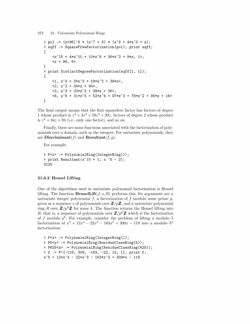
372 21. Univariate Polynomial Rings
> pol := (z+96)^6 * (z^7 + 9) * (z^8 + 4*z^3 + z);> sqff := SquareFreeFactorization(pol); print sqff;[
<z^15 + 4*z^10 + 10*z^8 + 36*z^3 + 9*z, 1>,<z + 96, 6>
]> print DistinctDegreeFactorization(sqff[1, 1]);[
<1, z^4 + 3*z^3 + 59*z^2 + 39*z>,<2, z^2 + 34*z + 94>,<3, z^3 + 33*z^2 + 39*z + 36>,<6, z^6 + 31*z^5 + 52*z^4 + 97*z^3 + 78*z^2 + 95*z + 16>
]
The final output means that the first squarefree factor has factors of degree1 whose product is z4 + 3z3 + 59z2 + 39z, factors of degree 2 whose productis z2 + 34z + 94 (i.e., only one factor), and so on.
Finally, there are some functions associated with the factorization of poly-nomials over a domain, such as the integers. For univariate polynomials, theyare Discriminant(f) and Resultant(f, g).
For example:
> P<x> := PolynomialRing(IntegerRing());> print Resultant(x^10 + 1, x ^5 - 2);3125
21.6.2 Hensel Lifting
One of the algorithms used in univariate polynomial factorization is Hensellifting. The function HenselLift(f, s, R) performs this. Its arguments are aunivariate integer polynomial f , a factorization of f modulo some prime p,given as a sequence s of polynomials over ZZ/pZZ, and a univariate polynomialring R over ZZ/pkZZ for some k. The function returns the Hensel lifting intoR, that is, a sequence of polynomials over ZZ/pkZZ which is the factorizationof f modulo pk. For example, consider the problem of lifting a modulo–5factorization of x5 + 12x4 − 22x3 − 163x2 + 309x − 119 into a modulo–54
factorization:
> P<x> := PolynomialRing(IntegerRing());> P5<y> := PolynomialRing(ResidueClassRing(5));> P625<z> := PolynomialRing(ResidueClassRing(625));> f := P![-119, 309, -163, -22, 12, 1]; print f;x^5 + 12*x^4 - 22*x^3 - 163*x^2 + 309*x - 119

21.6 Factorization and Root-Finding 373
Firstly, a factorization s of f modulo 5 is required. It may be found byapplying Factorization to the coercion of f into P5 :
> fact5 := Factorization(P5!f); print fact5;[
<y + 3, 1>,<y^2 + 2*y + 3, 1>,<y^2 + 2*y + 4, 1>
]> s := [t[1]: t in fact5]; print s;[
y + 3,y^2 + 2*y + 3,y^2 + 2*y + 4
]> print &*s eq P5!f;true
Now the Hensel lifting can take place:
> h625 := HenselLift(f, s, P625); print h625;[
z + 133,z^2 + 12*z + 618,z^2 + 492*z + 174
]> print &*h625 eq P625!f;true
The object of Hensel lifting is generally to find an integer polynomial fac-torization. If pk
2 ≥ 2n√∑n
i=0 f2i , where n is the degree of f , then the lifted
sequence should correspond fairly directly to an integer factorization of f .This is the case for the lifted sequence in the current example:
> print 625/2 ge> (2^n * Sqrt(&+[Coefficient(f, i): i in [0..n]])> where n is Degree(f));true
There is a slight complication, however, because when Magma coerces el-ements of residue rings modulo b into the integers, it always returns non-negative integers. Here what is wanted is the symmetric form, the rep-resentation ranging from −b b
2c to b b2c. The function defined below will
do the task. Given an integer polynomial f , it returns the correspond-ing integer polynomial with the coefficients in ‘symmetric form’ modulo b,

374 21. Univariate Polynomial Rings
that is, congruent modulo b to the original coefficients and in the range−(b div 2) .. + (b div 2):
> SymmetricForm := func< f, b |> Parent(f) ! [ cmod gt b div 2 select cmod-b else cmod> where cmod is c mod b : c in Coefficients(f) ] >;
> ipoly := [SymmetricForm(P!p, 625): p in h625];> print ipoly;[
x + 133,x^2 + 12*x - 7,x^2 - 133*x + 174
]
Now each factor of f is either a polynomial in ipoly , or a product of some ofthese polynomials (with SymmetricForm applied to the result):
> print [j: j in [1..3] | IsZero(f mod ipoly[j])];[ 2 ]> // so ipoly[2] is a factor> pr := SymmetricForm(ipoly[1] * ipoly[3], 625);> print f mod pr;0> print f eq ipoly[2] * pr;true> print ipoly[2], pr;x^2 + 12*x - 7x^3 - 15*x + 17
Hence the factorization of f over the integers is (x2 +12x−7)(x3−15x+17).
21.6.3 Roots of Univariate Polynomials
Let f be a univariate polynomial over the ring R, where R may be ZZ, Q, IR,C, GF(q) or ZZ/pZZ. A root of f is an object r such that when r is substitutedfor the indeterminate of f , the result is zero; unless otherwise stated, it isunderstood that r is an element of R. The function Roots(f) returns all theroots of f in R, in a format similar to a factorization sequence, that is, asa sequence of tuples < ri,mi > where ri is a root and mi is its multiplicity.(There is a slight exception: if f is over the free real field, then the return valuemay include complex roots.) For example, let f be the polynomial shownbelow. Its roots in Q are 3 (with multiplicity 2) and − 7
2 (with multiplicity1):
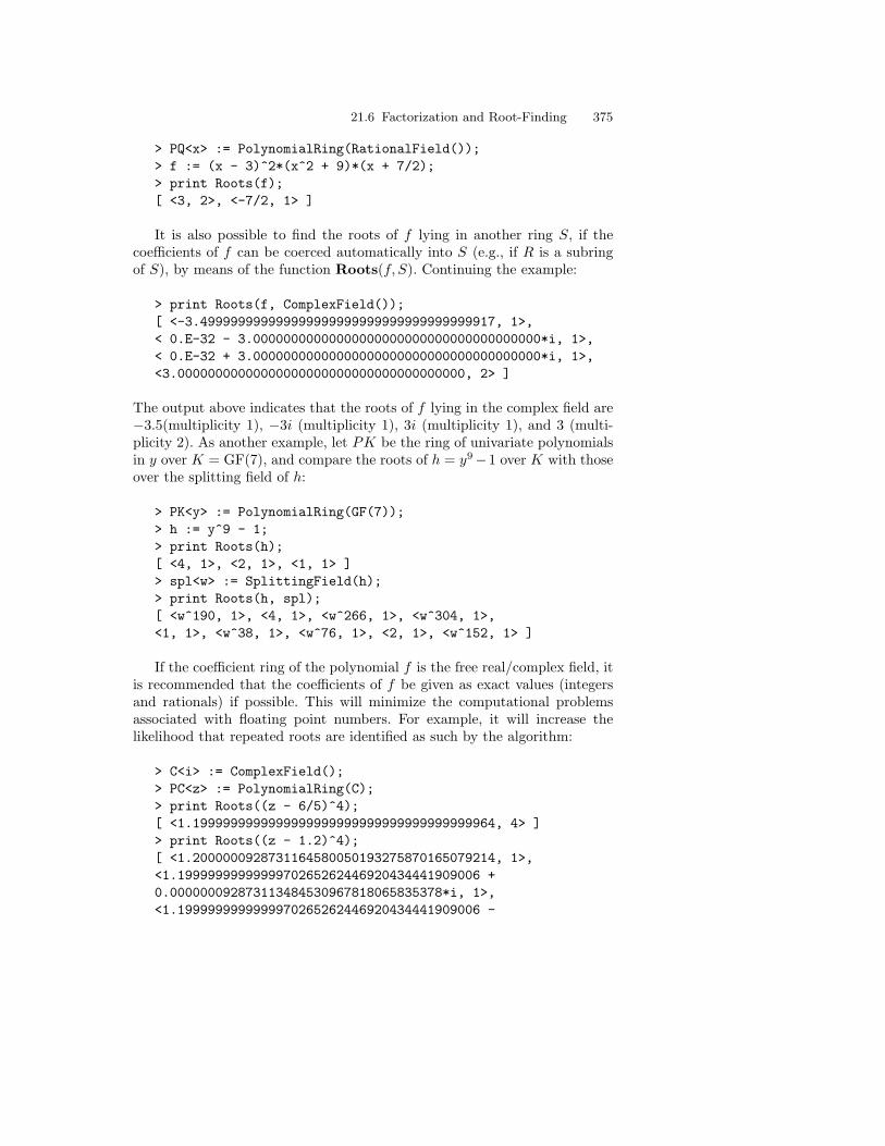
21.6 Factorization and Root-Finding 375
> PQ<x> := PolynomialRing(RationalField());> f := (x - 3)^2*(x^2 + 9)*(x + 7/2);> print Roots(f);[ <3, 2>, <-7/2, 1> ]
It is also possible to find the roots of f lying in another ring S, if thecoefficients of f can be coerced automatically into S (e.g., if R is a subringof S), by means of the function Roots(f, S). Continuing the example:
> print Roots(f, ComplexField());[ <-3.499999999999999999999999999999999999917, 1>,< 0.E-32 - 3.00000000000000000000000000000000000000*i, 1>,< 0.E-32 + 3.00000000000000000000000000000000000000*i, 1>,<3.00000000000000000000000000000000000000, 2> ]
The output above indicates that the roots of f lying in the complex field are−3.5(multiplicity 1), −3i (multiplicity 1), 3i (multiplicity 1), and 3 (multi-plicity 2). As another example, let PK be the ring of univariate polynomialsin y over K = GF(7), and compare the roots of h = y9−1 over K with thoseover the splitting field of h:
> PK<y> := PolynomialRing(GF(7));> h := y^9 - 1;> print Roots(h);[ <4, 1>, <2, 1>, <1, 1> ]> spl<w> := SplittingField(h);> print Roots(h, spl);[ <w^190, 1>, <4, 1>, <w^266, 1>, <w^304, 1>,<1, 1>, <w^38, 1>, <w^76, 1>, <2, 1>, <w^152, 1> ]
If the coefficient ring of the polynomial f is the free real/complex field, itis recommended that the coefficients of f be given as exact values (integersand rationals) if possible. This will minimize the computational problemsassociated with floating point numbers. For example, it will increase thelikelihood that repeated roots are identified as such by the algorithm:
> C<i> := ComplexField();> PC<z> := PolynomialRing(C);> print Roots((z - 6/5)^4);[ <1.1999999999999999999999999999999999999964, 4> ]> print Roots((z - 1.2)^4);[ <1.2000000928731164580050193275870165079214, 1>,<1.1999999999999970265262446920434441909006 +0.000000092873113484530967818065835378*i, 1>,<1.1999999999999970265262446920434441909006 -

376 21. Univariate Polynomial Rings
0.000000092873113484530967818065835378*i, 1>,<1.1999999071268894889424912882655105927445, 1> ]
Furthermore, if f is over the free real/complex field, then the user mayspecify the algorithm to be used, by means of the parameter Al. The de-fault value of Al is the string "Schonhage", which gives Xavier Gour-don’s implementation of Schonhage’s algorithm. Other possibilities for Alare "Laguerre", "NewtonRaphson", and "Combination" (a combination ofthe Laguerre and Newton-Raphson algorithms. The function Roots has asecond parameter, Digits, which is used to specify the desired accuracy dfor the calculation; the default value of d is the current precision of the freereal field. When Schonhage’s algorithm is used, the results will be correct towithin an absolute error of 10−d; for the other algorithms, an attempt willbe made to find the roots to an accuracy of d significant figures, but this isnot guaranteed.
If the coefficients of f are non-exact elements of the free real/complex field,then it may be preferable to use an alternative function, RootsNonExact(f),which is specially designed for this situation. It has a parameter Digits (de-fault value being the current precision of the free real field) whose value dis used to specify the accuracy required. RootsNonExact returns two se-quences [v1, . . . , vn] and e1, . . . , en], each containing elements of the free com-plex field. (Note that the multiplicities of the roots are not provided.) The vi
are approximations to the roots of f , such that |f − a(z − v1) . . . (z − vn)| <10−d|f |, where a is the leading coefficient of f . The ei provide error bounds,having the property that if f is any polynomial such that |f − f | < 10−d|f |,then one can write f = a(z − u1) . . . (z − un) with |vi − ui| < ei. In somecases, the second sequence will not be returned, because d is too small (forthe given polynomial) for such error bounds to be derived. Increasing d willdecrease the errors on the ‘roots’, but for meaningful answers any non-exactcoefficients of f must be given with at least d decimal places. For example:
> rts, errs := RootsNonExact((z - 6/5)^4);> print rts;[ 1.199999999999999999999999999984,1.199999999999999999999999999984,1.2000000000000000000000000000000000000023 -2.028356533497 E-19*i,1.2000000000000000000000000000000000000023 +2.028356533497 E-19*i ]> print errs;[ 0.0000005722045898, 0.0000005722045898,0.0000005722045898, 0.0000005722045898 ]

22. Multivariate Polynomial Rings
Multivariate polynomial rings and their ideals deal with the subject of Com-mutative Algebra which has a much larger theory than that associated withunivariate polynomial rings and their ideals. Consequently, the two typesof polynomial rings are implemented with different categories and althoughthey share many simple operations, the major algorithms are quite distinct.See Chapter 21 for more discussion of the differences between univariate andmultivariate polynomial rings.
Multivariate polynomials themselves are quite different from univariatepolynomials in that they are linearly ordered sums of coefficient-monomialpairs. Furthermore, the orderings on the monomials within the polynomialsplay an extremely significant role. Also central to computation with mul-tivariate polynomial rings is the concept of the Grobner basis, which is acanonical generating set of an ideal. The Buchberger Algorithm allows thecomputation of the Grobner basis of any ideal.
The category of multivariate polynomial rings is RngMPol.
22.1 Polynomial Rings and Monomial Orders
Let P be the multivariate polynomial ring R[x1, . . . , xn] of rank n over thecoefficient ring R. A monomial (or power product) of P is a product of powersof the variables of P ; that is, an expression of the form xe1
1 · · ·xenn with ei ≥ 0
for 1 ≤ i ≤ n. A term of P is a product cm where c is a coefficient from R andm is a monomial of P . Let M be the set of all monomials of P . A monomialordering on M is a total order < on M such that 1 ≤ s for all s ∈ M , s ≤ timplies su ≤ tu for all s, t, u ∈ M , and M is a well-ordering (every non-empty subset of M possesses a minimal element with respect to <). WithinMagma, each multivariate polynomial ring P has a fixed monomial order <associated with it.
The main function to create a multivariate polynomial ring in Magma isPolynomialRing(R,n, S) which takes the coefficient ring R, the rank n, and

378 22. Multivariate Polynomial Rings
the string S specifying the monomial order <. These arguments are optionallyfollowed by extra arguments associated with the particular monomial order.Two of the most important monomial orders are the lexicographical orderand the graded-reverse-lexicographical order.
The lexicographical order < (abbreviated lex) is defined for monomialss and t as follows: s < t iff there exists 1 ≤ i ≤ n such that the first i − 1exponents of s and t are equal but the i-th exponent of s is less than thei-th exponent of t. The order is called ‘lexicographical’ since it orders themonomials as if they were words in a dictionary. The i-th variable is greaterthan the (i + 1)-th variable for 1 ≤ i < n so the first variable is the greatestvariable. This order is specified by the string "lex" as the third argument tothe PolynomialRing function.
The graded-reverse-lexicographical order < (abbreviated grevlex) is de-fined for monomials s and t as follows: s < t iff the total degree of s is lessthan the total degree of t or the total degree of s is equal to the total degree oft and s > t with respect to the lexicographical order applied to the exponentsof s and t in reverse order. The order is called ‘graded reverse lexicograph-ical’ since it first grades the monomials by total degree, and then decidesties by the negation of the lexicographical order applied to the variables inreverse order. Again, the i-th variable is greater than the (i + 1)-th variablefor 1 ≤ i < n, so the first variable is the greatest variable. This order is speci-fied by the string "grevlex" as the third argument to the PolynomialRingfunction.
Other monomial orders available in Magma are the following: graded lex-icographical (glex), elimination (elim), inverse block (invblock), univariate(univ) and weight (weight). See the Handbook for details.
A polynomial f of P consists of a linearly ordered sum (internally, a linkedlist) of terms (i.e., coefficient-monomial pairs) such that the monomials of fare distinct and are sorted with respect to the specific monomial order withthe greatest monomial is first.
The following example constructs the polynomial ring of rank 3 over theinteger ring in two different ways, so as to illustrate the differences betweenthe lex and grevlex order. Note that generator assignment may be used togives names to the indeterminates:
> P<x, y, z> := PolynomialRing(IntegerRing(), 3, "lex");> print x + y + z;x + y + z> print x + y^20 + z^10*x^9;x^9*z^10 + x + y^20> print (x+y+z)^4;x^4 + 4*x^3*y + 4*x^3*z + 6*x^2*y^2 + 12*x^2*y*z + 6*x^2*z^2 +

22.2 Polynomial Creation and Access 379
4*x*y^3 + 12*x*y^2*z + 12*x*y*z^2 + 4*x*z^3 + y^4 +4*y^3*z + 6*y^2*z^2 + 4*y*z^3 + z^4
> P<x, y, z> := PolynomialRing(IntegerRing(), 3, "grevlex");> print x + y + z;x + y + z> print x + y^20 + z^10*x^9;y^20 + x^9*z^10 + x> print (x+y+z)^4;x^4 + 4*x^3*y + 6*x^2*y^2 + 4*x*y^3 + y^4 + 4*x^3*z +
12*x^2*y*z + 12*x*y^2*z + 4*y^3*z + 6*x^2*z^2 +12*x*y*z^2 + 6*y^2*z^2 + 4*x*z^3 + 4*y*z^3 + z^4
Since the lexicographical order is so important and is usually the orderdesired, it is the one used if the order argument is omitted. Thus the state-ments
> P<x, y, z> := PolynomialRing(IntegerRing(), 3, "lex");
and
> P<x, y, z> := PolynomialRing(IntegerRing(), 3)
have exactly the same effect.
Note that a multivariate polynomial ring of rank 1 over the coefficientring R is not the same as the univariate polynomial ring over R. The opera-tions applicable to the former are those discussed in this chapter while thoseapplicable to the latter are discussed in Chapter 21. Usually, if one wishesto compute with univariate polynomials then the univariate polynomial ringshould be used (particularly since there are many functions applicable to uni-variate polynomials which would be useful), and the multivariate polynomialring of rank 1 should only be used when it occurs, say, as the base case of arecursive algorithm which computes with multivariate polynomial rings.
22.2 Polynomial Creation and Access
The only way to create a multivariate polynomial in Magma is to use anexpression in the indeterminates, or to coerce an element of the coefficientring into the polynomial ring to create a constant polynomial.
For example, the following lines create the element c = 4s3 + 20s2t +19st4 + 8t + 7 in the polynomial ring P = Q[s, t]:
> P<s, t> := PolynomialRing(RationalField(), 2);

380 22. Multivariate Polynomial Rings
> c := 20*s^2*t + 4*s^3 - 12*s*t^4 + 8*t - 24;> print c;4*s^3 + 20*s^2*t + 19*s*t^4 + 8*t + 7
Magma provides a large number of functions for accessing multivari-ate polynomials. These functions are quite different from those applicableto univariate polynomials because the multivariate polynomials have quite adifferent structure as linearly ordered sums.
Since a multivariate polynomial f is just a linearly ordered sum ofcoefficient-monomial pairs, f can be viewed in an absolute manner as twoparallel lists: the list of base coefficients (from the coefficient ring) and thelist of monomials. Note that in this viewpoint, the sequence of base coef-ficients on its own is useless since it only corresponds to the sequence ofmonomials. Table 22.1 lists the functions for accessing polynomials in theabsolute manner.
Table 22.1. Absolute access functions for multivariate polynomials
Magma Meaning
Coefficients(f) Coefficients of f as a sequence
LeadingCoefficient(f) Leading coefficient of f
TrailingCoefficient(f) Trailing coefficient of f
MonomialCoefficient(f, m) Coefficient of monomial m in f
Monomials(f) Monomials of f as a sequence
LeadingMonomial(f) Leading monomial of f
Terms(f) Terms of f as a sequence
LeadingTerm(f) Leading term of f
TrailingTerm(f) Trailing term of f
TotalDegree(f) Total degree of f (maximum of total degrees ofmonomials of f)
LeadingTotalDegree(f) Total degree of leading monomial of f
For a fixed variable v, a multivariate polynomial f may be viewed recur-sively as a univariate polynomial with respect to variable v. That is, f may beconsidered as a linearly ordered sum whose terms are of the form civ
i whereci is the coefficient of the power vi, which is still in general a polynomial (notcontaining v though, of course). Magma provides functions to access f con-sidered in this way. For each function the variable v can be specified in twoways: as the integer i ∈ 1 . . . n (where n is the rank of the ring) which is thevariable number which corresponds to v, or as the variable v itself (lying inthe polynomial ring). Table 22.2 lists the functions for accessing polynomials

22.2 Polynomial Creation and Access 381
in the recursive manner. The functions are only listed in the form in whichthe variable number i is given; for each function there is also a version whichtakes the actual variable v instead of the number i.
Table 22.2. Recursive access functions for multivariate polynomials
Magma Meaning
Coefficients(f, i) (Recursive) coefficients of f w.r.t. variable num-ber i as a sequence
Coefficient(f, i, k) k-th (recursive) coefficient of f w.r.t. variablenumber i as a polynomial
LeadingCoefficient(f, i) (Recursive) leading coefficient of f w.r.t. variablenumber i
TrailingCoefficient(f, i) (Recursive) trailing coefficient of f w.r.t. variablenumber i
Terms(f, i) (Recursive) terms of f w.r.t. variable number i asa sequence
Term(f, i, k) (Recursive) k-th term of f w.r.t. variable numberi
LeadingTerm(f, i, k) (Recursive) leading term of f w.r.t. variable num-ber i
TrailingTerm(f, i, k) (Recursive) leading term of f w.r.t. variable num-ber i
Degree(f, i) (Recursive) degree of f w.r.t. variable number i
The following example demonstrates the differences between the abso-lute and recursive access functions for a polynomial ring with lex monomialordering:
> P<x, y, z> := PolynomialRing(IntegerRing(), 3);> f := 2*x^3*y*z + 4*y*z^3 + 8*z + 3;> print f;2*x^3*y*z + 4*y*z^3 + 8*z + 3> print Coefficients(f);[ 2, 4, 8, 3 ]> print Monomials(f);[
x^3*y*z,y*z^3,z,1
]> print Terms(f);[

382 22. Multivariate Polynomial Rings
2*x^3*y*z,4*y*z^3,8*z,3
]> print TotalDegree(f);5> print LeadingMonomial(f);x^3*y*z> print Degree(f, x);3> print Coefficients(f, x);[
4*y*z^3 + 8*z + 3,0,0,2*y*z
]> print Coefficient(f, x, 0);4*y*z^3 + 8*z + 3
22.3 Factorization, Resultants and Derivatives
Magma incorporates powerful algorithms for factoring multivariate polyno-mials over various coefficient rings. Currently, the available coefficient ringsare: the integer ring ZZ; the rational field Q; finite fields; cyclotomic, quadratic,and general number fields; and rational function fields or polynomial ringsover any of the above.
The factorization algorithms for multivariate polynomials are generallymuch harder than the corresponding ones for univariate polynomials. Indeed,the easiest coefficient rings for univariate polynomials are the finite fields,while for multivariate polynomials the finite fields become the most difficultcoefficient rings!
The function Factorization(f) factorizes the polynomial f into powersof irreducible polynomials. The factorization is actually computed for thecanonical associate f ′ of f and the unit u such that f = uf ′ is also returned.For a polynomial f with coefficient ring a field, f ′ is the monic polynomialassociated with f while for a polynomial f with coefficient ring ZZ, f ′ is theassociate of f with positive leading coefficient. For example:
> P<x, y, z> := PolynomialRing(RationalField(), 3);

22.3 Factorization, Resultants and Derivatives 383
> f := 5 * (x^2 + y + z)*(x + y^2 + z)*(x + y + z^2)^2;> print f;5*x^5 + 5*x^4*y^2 + 10*x^4*y + 10*x^4*z^2 + 5*x^4*z +
10*x^3*y^3 + 10*x^3*y^2*z^2 + 5*x^3*y^2 + 10*x^3*y*z^2 +10*x^3*y*z + 5*x^3*y + 5*x^3*z^4 + 10*x^3*z^3 + 5*x^3*z+ 5*x^2*y^4 + 10*x^2*y^3*z^2 + 5*x^2*y^3 + 5*x^2*y^2*z^4+ 10*x^2*y^2*z + 10*x^2*y^2 + 10*x^2*y*z^3 +10*x^2*y*z^2 + 15*x^2*y*z + 5*x^2*z^5 + 10*x^2*z^3 +5*x^2*z^2 + 10*x*y^4 + 10*x*y^3*z^2 + 10*x*y^3*z +5*x*y^3 + 10*x*y^2*z^3 + 10*x*y^2*z^2 + 15*x*y^2*z +5*x*y*z^4 + 20*x*y*z^3 + 10*x*y*z^2 + 5*x*z^5 + 10*x*z^4+ 5*y^5 + 10*y^4*z^2 + 5*y^4*z + 5*y^3*z^4 + 10*y^3*z^3+ 5*y^3*z + 5*y^2*z^5 + 10*y^2*z^3 + 5*y^2*z^2 + 5*y*z^5+ 10*y*z^4 + 5*z^6
> F, u := Factorization(f);> print F, u;[
<x + y + z^2, 2>,<x + y^2 + z, 1>,<x^2 + y + z, 1>
]5
The function IsIrreducible(f) returns true if and only if the polynomialf is irreducible. Another factorization function is SquareFreeFactorization(f).It returns the square-free factorization (with appropriate unit) of the canon-ical associate f ′ of f which is a factorization sequence of square-free (but notnecessarily irreducible) factors with their multiplicities. None of the factorswill contain the square of any non-constant polynomial. For example:
> P<x, y, z> := PolynomialRing(IntegerRing(), 3);> f := (x + y + z)^2 * (x^2 - y^2)^3;> print f;x^8 + 2*x^7*y + 2*x^7*z - 2*x^6*y^2 + 2*x^6*y*z + x^6*z^2 -
6*x^5*y^3 - 6*x^5*y^2*z - 6*x^4*y^3*z - 3*x^4*y^2*z^2 +6*x^3*y^5 + 6*x^3*y^4*z + 2*x^2*y^6 + 6*x^2*y^5*z +3*x^2*y^4*z^2 - 2*x*y^7 - 2*x*y^6*z - y^8 - 2*y^7*z -y^6*z^2
> print SquareFreeFactorization(f);[
<x + y + z, 2>,<x^2 - y^2, 3>
]> print Factorization(f);[

384 22. Multivariate Polynomial Rings
<x - y, 3>,<x + y, 3>,<x + y + z, 2>
]
The function Resultant(f, g, i) returns the resultant of polynomials fand g with respect to the i-th variable while the function Resultant(f, g, v)returns the resultant of polynomials f and g with respect to variable v. Sim-ilarly, the functions Discriminant(f, i) and Discriminant(f, v) computethe discriminant of f with respect to the appropriate variable. For example,the following statements compute the resultant of two bivariate polynomialswith respect to one variable. Note that the resultant can also be computedin this case by an elimination ideal computation (see Section 22.8 below).
> P<x,y> := PolynomialRing(RationalField(), 2);> f := x^5 + y^2 + 1;> g := y^3 + x + 3;> print Resultant(f, g, y);x^15 + 3*x^10 + 3*x^5 + x^2 + 6*x + 10> print I := ideal<P | f, g>;> I;Ideal of Polynomial ring of rank 2 over Rational FieldLexicographical OrderVariables: x, yBasis:[
x^5 + y^2 + 1,x + y^3 + 3
]> print EliminationIdeal(I, x);Ideal of Polynomial ring of rank 2 over Rational FieldLexicographical OrderVariables: x, yBasis:[
x^15 + 3*x^10 + 3*x^5 + x^2 + 6*x + 10]
The functions Derivative(f, i) and Derivative(f, v) compute the for-mal derivative of f with respect to the appropriate variable. Similarly, thefunctions Integral(f, i) and Integral(f, v) compute the formal integral of fwith respect to the appropriate variable.

22.4 Multivariate Function Fields 385
22.4 Multivariate Function Fields
A multivariate rational function field F of rank n over the ring R is thefield of fractions of a multivariate polynomial ring P of rank n over the ringR. That is, it consists of fractions whose numerator and denominator arepolynomials over R with n indeterminates. The polynomial ring P is calledthe ring of integers of F . There are two ways to create the field F . GivenP , FieldOfFractions(P ) returns F . Alternatively, FunctionField(R, n)returns F , using the lexicographical monomial order for P . The functionIntegerRing(F ) returns P .
As in the univariate case, if t = nd is an element of a multivariate func-
tion field, where a and b are expressed in lowest terms, then Numerator(t)and Denominator(t) return n and d as elements of the corresponding ringof integers (i.e., the polynomial ring). These functions behave similarly forelements of the rational field.
It is often useful to give the same indeterminate names to the polynomialring and then to the function field. For example:
> P6<a,b,c,d,e,f> := PolynomialRing(RationalField(), 6);> F6<a,b,c,d,e,f> := FieldOfFractions(P6);
The effect of this is subtle. After the two generator assignments, the print-names for both magmas are a, b, c, d, e, f , so that the natural identificationcan be made in the output. However, the second and final time that theidentifiers a, b, c, d, e, f are assign ed, they are given the indeterminates ofF6 as their values, so that in subsequent expressions they will refer to theseelements. For instance:
> t := 14*a + c;> print t;14*a + c> print Parent(t);Rational function field of rank 6 over Rational FieldVariables: a, b, c, d, e, f> num := Numerator(t); print num;14*a + c> print Parent(num);Polynomial ring of rank 6 over Rational FieldLexicographical OrderVariables: a, b, c, d, e, f
Rational functions in several indeterminates may be used for perform-ing algebraic manipulations. For instance, one way of solving the system of

386 22. Multivariate Polynomial Rings
simultaneous equations
ax + by = e
cx + dy = f
which can be written in matrix form as
(x y
) (a c
b d
)=
(e f
)
is to calculate the inverse of the coefficient matrix and multiply the vectorof constants by this inverse. This can always be done using the functionfield since the determinant ad − bc is a non-zero element of the field, so theinverse exists. If in a particular assignment of the variables a, b, c, d, e, f thisdeterminant remains non-zero, then the solution derived from the functionfield remains valid. In Magma, all of these operations can be done in termsof the function field F6 defined above:
> coeffmat := MatrixRing(F6, 2)![a, c, b, d];> print coeffmat;[a c][b d]> rhs := VectorSpace(F6, 2)![e, f];> print rhs;(e f)> print rhs * coeffmat^-1;((-b*f + d*e)/(a*d - b*c) (a*f - c*e)/(a*d - b*c))
The output equals the vector(
x y). Therefore the solution is
x =−bf + de
ad− bc, y =
af − ce
ad− bc,
assuming the determinant ad− bc is non-zero. (If the determinant were zero,the solution could be obtained easily by another method.) This example canof course be generalized to much larger examples, and also to non-linearexamples, as shown in the following sections.
22.5 Ideals
In this section, assume that P is a polynomial ring in n variables over thefield K.

22.5 Ideals 387
For an ideal I of the polynomial ring P , a basis B of I is an (ideal)generating set of I, i.e., a subset of I such that any element of I can beexpressed as a finite sum of products of the form fg where f ∈ P and g ∈ B.The Hilbert Basis Theorem states that every ideal I possesses a finite basis.Within Magma, a basis of an ideal I is in fact an ordered sequence of elementsof I, possibly with repetitions. Thus a basis of an ideal is different from, say,a vector space basis since it may contain repetitions and zero elements.
The most simple but important problem associated with an ideal is themembership test: given a polynomial f ∈ P and an ideal I of P , is f ∈ I? Toanswer this question, a multivariate division algorithm will be developed.
Suppose B is a basis of an ideal I of P and f ∈ P . If f is non-zero, fis said to be top-reducible with respect to B if there exists a g ∈ B suchthat the leading monomial (greatest monomial with respect to the monomialordering) of g divides the leading monomial of f . If such a case holds, thenf can be reduced by g by subtracting the appropriate multiple of g from fwhich cancels the leading term of f . It is easy to show from the propertiesof the monomial order that the leading monomial of the new polynomialf1 (if non-zero) is strictly less than that of f . If the new polynomial f1 isnon-zero yet also top-reducible with respect to B, the same procedure canbe applied to it to yield f2, and so on until an fk is reached which is eitherthe zero polynomial or is non-zero but is not top-reducible with respect toB. The process does terminate because a monomial order is a well-ordering.The polynomial fk is called a normal form of f with respect to the basis B.(If f is already zero, then f is a (in fact, the only) normal form of f .)
If a normal form of a polynomial f ∈ P with respect to the basis B iszero, then it is easy to see that f ∈ I. However, the converse is in generalfalse; i.e., it is possible that a polynomial f is in the ideal I yet a normal formof f with respect to B is non-zero. As an example, let P be the polynomialring Q[x, y, z] with lexicographical order and x > y > z, let B be the basisx + y, x + z, and let I be the ideal generated by B. Then the polynomialf = y − z is obviously in I yet a normal form of it with respect to B is stillf since the leading monomials x and x respectively of the polynomials of Bdo not divide the leading monomial y of f .
The notion of Grobner basis was introduced to remedy this problem: abasis B of a polynomial ideal I of P is called a Grobner basis if, for allf ∈ P , f ∈ I if and only if every normal form of f with respect to B iszero. The Buchberger Algorithm takes an arbitrary basis B of an ideal I andconstructs a Grobner basis for I. This algorithm is of central importanceto all computations with ideals of multivariate polynomial rings. A Grobnerbasis for an ideal with respect to a fixed monomial order can also be put intoa unique form, just like the unique reduced-row echelon form of a matrix.(The basis is minimalized, reduced and sorted—see [CLO92], Chapter 2, §7

388 22. Multivariate Polynomial Rings
for details.) This is always done in Magma so that every ideal I possesses aunique Grobner basis since it has a fixed monomial order.
Table 22.3. Ideal creation and basis functions
Magma Meaning
ideal< P | L > Ideal of P generated by polynomials in L
ideal(Q) Ideal with user basis Q
Basis(I) Current basis of I
BasisElement(I, i) i-th element of the basis of I
Coordinates(I, f) Coordinates of f ∈ I with respect to the basis of I
Groebner(I) Procedure explicitly forcing a Grobner basis to be con-structed for I
GroebnerBasis(I) (Unique) Grobner basis of ideal I
GroebnerBasis(S) (Unique) Grobner basis of the ideal generated by set orsequence S
Magma incorporates an efficient implementation of the Buchberger Al-gorithm which is automatically invoked when necessary. The usual way tocreate an ideal is by the ideal constructor which is given the polynomialring P (or an over-ideal) on the left side, and a list on the right side whichdescribes a basis for an ideal. Magma remembers the original basis as con-structed as the current basis for the ideal until it needs a Grobner basis: atthat point it changes the current basis to the unique Grobner basis of thatideal and discards the original basis. To force Magma to explicitly computethe Grobner basis of an ideal I, the procedure Groebner(I) may be invoked.Note that it is never actually necessary to do this for any ideal computations– Magma will automatically compute the Grobner basis if it needs to do so.
For example:
> P<x, y, z> := PolynomialRing(RationalField(), 3);> I := ideal<P | x + y, x + z>;> print I;Ideal of Polynomial ring of rank 3 over Rational FieldLexicographical OrderVariables: x, y, zBasis:[
x + y,x + z
]> print (y-z) in I;true

22.5 Ideals 389
> print I; // NB: Groebner basis of I is now knownIdeal of Polynomial ring of rank 3 over Rational FieldLexicographical OrderVariables: x, y, zGroebner basis:[
x + z,y - z
]
Table 22.3 lists the functions for creating ideals and accessing their bases.Note that it is possible by the Ideal(Q) function to create an ideal with abasis such that the basis is remembered by Magma so that polynomials ofthe ideal can be written in terms of this basis by the Coordinates(I, f)function—see the Handbook for details.
Verbose output for the Buchberger Algorithm (invoked, for example, di-rectly by the Groebner procedure) can be obtained by the procedure callSetVerbose("Groebner", 1).
Magma incorporates an implementation of the exciting new GrobnerWalk algorithm for changing the Grobner basis of an ideal with respect toone monomial order to the Grobner basis of the ideal with respect to an-other monomial order (see [CKM96]). This gives a very powerful method inMagma for computing the Grobner basis of the fixed monomial order of anideal: first the Grobner basis of the ideal is computed with respect to an easyorder (usually the grevlex order) by the plain Buchberger Algorithm, andthen the Grobner Walk algorithm is invoked to convert this Grobner basisto the Grobner basis with respect to the desired final order. Generally thismethod is much faster than by using the plain Buchberger Algorithm directlywith the final desired order. The method is automatically employed withinMagma whenever a Grobner basis is needed. The ChangeOrder functionallows one to manually apply the Grobner Walk algorithm as desired—seethe Handbook for details.
Occasionally the above method using the Grobner Walk can be slowerthan the method of using the plain Buchberger Algorithm directly with thefinal desired order. To circumvent this problem, the parameter Walk for theGroebner function can be used to control the method. Thus if I is anideal, then the procedure call Groebner(I : Walk := false) will constructthe Grobner basis for the ideal I without using the Grobner Walk algorithmand will just use the plain Buchberger Algorithm directly with the final de-sired order.
Verbose output for the Grobner Walk algorithm can be obtained by theprocedure call SetVerbose("GroebnerWalk", 1). The verbose output indi-

390 22. Multivariate Polynomial Rings
cates each of the steps followed by the algorithm. The verbose output for theBuchberger algorithm is automatically turned off within the Grobner Walkalgorithm since it is called frequently with relatively trivial input. Settingthe verbose level to be 2 enables the verbose printing for the Buchbergeralgorithm as well.
22.6 Ideal Access and Arithmetic
Since ideals of multivariate polynomials are general ideals (and rings) in them-selves, many common ideal operations can be performed on them. Table 22.4lists the basic access and arithmetic functions for multivariate polynomial ide-als. The table also lists some operations which can be done on polynomialswith respect to an ideal.
An example to demonstrate the ideal arithmetic functions:
> P<x, y, z> := PolynomialRing(GF(2), 3);> I := ideal<P | x^2 + y^2, (y + z)^3 - 1>;> J := ideal<P | x^2 + y^2, y + z>;> M := I meet J;> print M;Ideal of Polynomial ring of rank 3 over GF(2)Lexicographical OrderVariables: x, y, zBasis:[
y^4 + y + z^4 + z,x^2 + y^2
]> print M subset I;true> print M subset J;true> print I * J eq M;true> print IsInRadical(x + y, I);true> print (x + y) in I;false> print (x + y)^2 in I;true> print ColonIdeal(J, ideal<P|x+y>);Ideal of Polynomial ring of rank 3 over GF(2)

22.7 Quotient Rings 391
Lexicographical OrderVariables: x, y, zBasis:[
x + y,y + z
]
Table 22.4. Ideal functions
Magma Meaning
I + J Sum of ideals I and J
I*J Product of ideals I and J
I^k k-th power of ideal I
ColonIdeal(I, J) Colon ideal or ideal quotient I : J
ColonIdeal(I, f) Colon ideal or ideal quotient I : f∞
I meet J Intersection of ideals I and J
&meet S Intersection of set/sequence S of ideals
Generic(I) Generic polynomial of which I is an ideal
I eq J True iff ideals I and J are equal
I subset J True iff ideal I is contained in ideal J
IsProper(I) True iff ideal I is a proper ideal
IsZero(I) True iff ideal I is the zero ideal
f in I True iff polynomial f is in ideal I
IsInRadical(f, I) True iff polynomial f is in the radical of ideal I
NormalForm(f, I) Normal form of polynomial f with respect to ideal I
SPolynomial(f, g) S-polynomial of polynomials f and g
22.7 Quotient Rings
For an ideal I of the polynomial ring P = K[x1, . . . , xn], it is possible toform the quotient ring Q = P/I. This can be done either by the / functionor by the quo constructor. The new indeterminates of the quotient ring canbe named by the angle bracket notation as usual.
For example, the following construction of a quotient ring Q:
> P<x, y, z> := PolynomialRing(RationalField(), 3);> Q<a, b, c> := quo<P | x^3 + y + z, x + y^3 + z,> x + y + z^3>;

392 22. Multivariate Polynomial Rings
is completely equivalent to the construction:
> P<x, y, z> := PolynomialRing(RationalField(), 3);> I := ideal<P | x^3 + y + z, x + y^3 + z, x + y + z^3>;> Q<a, b, c> := P / I;
The quotient ring Q consists of the residues (normal forms) of the elementsof P with respect to the ideal I. Obviously Q has the structure of a vectorspace over the field K, just like P has.
An extremely important case arises when the dimension of Q as a vec-tor space over K is finite. In such a case, Magma provides the functionVectorSpace(Q) to create a vector space V together with an isomorphismf from Q onto V . This is useful for investigating further structural propertiesof Q. Table 22.5 lists the functions for computing with quotient rings.
Table 22.5. Quotient ring functions
Magma Meaning
CoefficientRing(Q) Coefficient ring of quotient ring Q
Rank(Q) Rank of quotient ring Q
Q.i i-th indeterminate of quotient ring Q
Dimension(Q) Dimension of quotient ring as vector space over K
VectorSpace(Q) Vector space isomorphic to Q together withisomorphism
MatrixAlgebra(Q) Matrix algebra isomorphic to Q together withisomorphism
Continuing the above example:
> print Dimension(Q);27> V, f := VectorSpace(Q);> // Print vector space basis of Q:> print [V.i@@f: i in [1..27]];[ 1, c, c^2, c^3, c^4, c^5, c^6, c^7, c^8, c^9, c^10, c^11,c^12, c^13, c^14, c^15, c^16, b, b*c, b*c^2, b*c^3, b*c^4,
b*c^5, b*c^6, b*c^7, b*c^8, b^2 ]
As well as the functions applicable for standard ring elements, the func-tions RepresentationMatrix(f), MinimalPolynomial(f), IsUnit(f), andIsNilpotent(f) may also be applied to elements of finite-dimensional quo-tient rings—see the Handbook for details.

22.8 Varieties and Elimination 393
For example, suppose the user wishes to find the minimal polynomial ofθ =
√2+ 3√
5 over Q. To do this, it suffices to calculate the minimal polynomialof (the residue class of) x+y over Q in the quotient ring Q[x, y]/(x2−2, y3−5):
> P<x, y> := PolynomialRing(RationalField(), 2);> Q<a, b> := quo<P | x^2 - 2, y^3 - 5>;> UP<t> := PolynomialRing(RationalField());> print MinimalPolynomial(a + b);t^6 - 6*t^4 - 10*t^3 + 12*t^2 - 60*t + 17
A further example to demonstrate the basic arithmetic in quotient ringswhen the quotient ring does not have finite dimension:
> P<x, y, z> := PolynomialRing(RationalField(), 3);> I := ideal<P | x^3 + y + z, x + y^3 + z>;> Groebner(I);> print I;Ideal of Polynomial ring of rank 3 over Rational FieldLexicographical OrderVariables: x, y, zGroebner basis:[
x + y^3 + z,y^9 + 3*y^6*z + 3*y^3*z^2 - y + z^3 - z
]> Q<a, b, c> := P / I;> print a;-b^3 - c> print b^8;b^8> print b^9;-3*b^6*c - 3*b^3*c^2 + b - c^3 + c> print c;c> print c^100;c^100
22.8 Varieties and Elimination
For an ideal I of the polynomial ring P = K[x1, . . . , xn], the variety of I isdefined to be the subset V of Kn consisting of all (a1, . . . , an) ∈ Kn suchthat f(a1, . . . , an) = 0 for all f ∈ I. Thus V is the set of solutions of thesimultaneous equations implied by the polynomials of I. It can be easily

394 22. Multivariate Polynomial Rings
shown that V is equal to the set of solutions of the simultaneous equationsimplied by the polynomials of any finite basis of I. In particular, a Grobnerbasis of I may be used.
For example, consider the system of equations Runge-Kutta 2 from thepaper [BGK86]. The coefficient field K is the rational function field Q(c2, c3),and the polynomial ring K[c4, b4, b3, b2, b1, a21, a31, a32, a41, a42, a43] has 11variables with the lexicographical ordering on monomials. After creating theideal I generated by these polynomials, a Grobner basis of I contains a linearpolynomial for each variable so there is exactly one solution to the systemgiven by the polynomials in the Grobner basis (i.e., the corresponding varietyhas size 1).
> K<c2,c3> := FunctionField(IntegerRing(), 2);> P<c4,b4,b3,b2,b1,a21,a31,a32,a41,a42,a43> :=> PolynomialRing(K, 11);> I := ideal<P |> b1 + b2 + b3 + b4 - 1,> b2*c2 + b3*c3 + b4*c4 - 1/2,> b2*c2^2 + b3*c3^2 + b4*c4^2 - 1/3,> b3*a32*c2 + b4*a42*c2 + b4*a43*c3 - 1/6,> b2*c2^3 + b3*c3^3 + b4*c4^3 - 1/4,> b3*c3*a32*c2 + b4*c4*a42*c2 + b4*c4*a43*c3 - 1/8,> b3*a32*c2^2 + b4*a42*c2^2 + b4*a43*c3^2 - 1/12,> b4*a43*a32*c2 - 1/24,> c2 - a21,> c3 - a31 - a32,> c4 - a41 - a42 - a43>;> Groebner(I);> print I;Ideal of Polynomial ring of rank 11 over
Rational function field of rank 2 over Integer RingVariables: c2, c3
Lexicographical OrderVariables: c4, b4, b3, b2, b1, a21, a31, a32, a41, a42, a43Dimension 0Groebner basis:[
c4 - 1,b4 + (-6*c2*c3 + 4*c2 + 4*c3 - 3)/(12*c2*c3 - 12*c2 -
12*c3 + 12),b3 + (2*c2 - 1)/(12*c2*c3^2 - 12*c2*c3 - 12*c3^3 +
12*c3^2),b2 + (-2*c3 + 1)/(12*c2^3 - 12*c2^2*c3 - 12*c2^2 +
12*c2*c3),
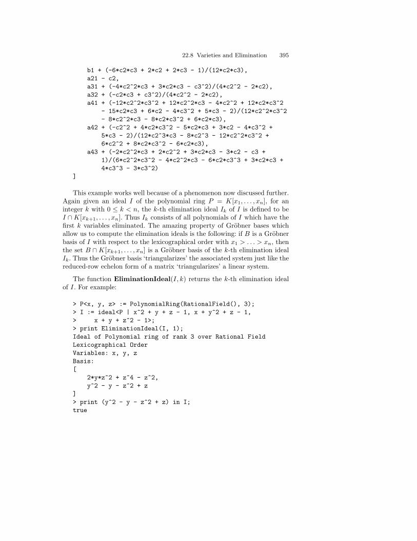
22.8 Varieties and Elimination 395
b1 + (-6*c2*c3 + 2*c2 + 2*c3 - 1)/(12*c2*c3),a21 - c2,a31 + (-4*c2^2*c3 + 3*c2*c3 - c3^2)/(4*c2^2 - 2*c2),a32 + (-c2*c3 + c3^2)/(4*c2^2 - 2*c2),a41 + (-12*c2^2*c3^2 + 12*c2^2*c3 - 4*c2^2 + 12*c2*c3^2
- 15*c2*c3 + 6*c2 - 4*c3^2 + 5*c3 - 2)/(12*c2^2*c3^2- 8*c2^2*c3 - 8*c2*c3^2 + 6*c2*c3),
a42 + (-c2^2 + 4*c2*c3^2 - 5*c2*c3 + 3*c2 - 4*c3^2 +5*c3 - 2)/(12*c2^3*c3 - 8*c2^3 - 12*c2^2*c3^2 +6*c2^2 + 8*c2*c3^2 - 6*c2*c3),
a43 + (-2*c2^2*c3 + 2*c2^2 + 3*c2*c3 - 3*c2 - c3 +1)/(6*c2^2*c3^2 - 4*c2^2*c3 - 6*c2*c3^3 + 3*c2*c3 +4*c3^3 - 3*c3^2)
]
This example works well because of a phenomenon now discussed further.Again given an ideal I of the polynomial ring P = K[x1, . . . , xn], for aninteger k with 0 ≤ k < n, the k-th elimination ideal Ik of I is defined to beI ∩K[xk+1, . . . , xn]. Thus Ik consists of all polynomials of I which have thefirst k variables eliminated. The amazing property of Grobner bases whichallow us to compute the elimination ideals is the following: if B is a Grobnerbasis of I with respect to the lexicographical order with x1 > . . . > xn, thenthe set B ∩K[xk+1, . . . , xn] is a Grobner basis of the k-th elimination idealIk. Thus the Grobner basis ‘triangularizes’ the associated system just like thereduced-row echelon form of a matrix ‘triangularizes’ a linear system.
The function EliminationIdeal(I, k) returns the k-th elimination idealof I. For example:
> P<x, y, z> := PolynomialRing(RationalField(), 3);> I := ideal<P | x^2 + y + z - 1, x + y^2 + z - 1,> x + y + z^2 - 1>;> print EliminationIdeal(I, 1);Ideal of Polynomial ring of rank 3 over Rational FieldLexicographical OrderVariables: x, y, zBasis:[
2*y*z^2 + z^4 - z^2,y^2 - y - z^2 + z
]> print (y^2 - y - z^2 + z) in I;true

396 22. Multivariate Polynomial Rings
The function EliminationIdeal(I, S), where S is a set of variables (orset of variable numbers) from the polynomial ring P , returns the eliminationideal I∩K[S]. This allows one to eliminate all variables except for the desiredones easily.
An ideal I of the polynomial ring P = K[x1, . . . , xn], is called zero-dimensional if the quotient ring Q = P/I has finite dimension as a vec-tor space over K. This definition is fundamental and arises in many con-texts. The function IsZeroDimensional(I) returns whether the ideal I iszero-dimensional. An alternative characterization is that an ideal I is zero-dimensional if and only if its variety over the algebraic closure of the coef-ficient field is finite. Yet another characterization of zero-dimensionality willbe given below in the section on dimension of ideals.
If an ideal I is zero-dimensional then the univariate elimination ideal I ∩K[xi] for each i = 1, . . . n will be non-trivial. There is a unique monic genera-tor of each ideal. Since it is of frequent importance to know these polynomials,Magma provides the function UnivariateEliminationIdealGenerator(I, i)to calculate the unique monic generator of the i-th univariate eliminationideal and the function UnivariateEliminationIdealGenerators(I) to cal-culate a sequence containing all n of these polynomials. Magma does all ofthis efficiently since it only needs to calculate one Grobner basis of the idealwith respect to an easy monomial order and it then applies the Grobner Walkto change this Grobner basis to the Grobner basis with respect to an elim-ination order which yields the desired polynomial. Note that this methodis generally much faster than the common method of using linear algebrapresented, for example, in [BeW93].For example:
> P<x, y, z> := PolynomialRing(RationalField(), 3);> I := ideal<P | x^3 + y + z - 1, x + y^2 + z - 1,> x + y + z^4 - 1>;> print I;Ideal of Polynomial ring of rank 3 over Rational FieldLexicographical OrderVariables: x, y, zBasis:[
x^3 + y + z - 1,x + y^2 + z - 1,x + y + z^4 - 1
]> print IsZeroDimensional(I);true> print UnivariateEliminationIdealGenerators(I);[
x^23 - 8*x^20 + 4*x^18 + 24*x^17 - 24*x^15 - 32*x^14 +

22.8 Varieties and Elimination 397
6*x^13 + 50*x^12 + 7*x^11 - 24*x^10 - 16*x^9 + 2*x^8+ 12*x^7 + 6*x^6 - 9*x^5 - x^3 + 2*x^2,
y^22 + y^21 - 11*y^20 - 11*y^19 + 55*y^18 + 51*y^17 -165*y^16 - 126*y^15 + 330*y^14 + 162*y^13 - 434*y^12- 96*y^11 + 342*y^10 + 66*y^9 - 180*y^8 - 111*y^7 +112*y^6 + 68*y^5 - 23*y^4 - 44*y^3 - y^2 + 14*y,
z^22 + z^21 + z^20 + z^19 - 5*z^18 - 5*z^17 - 5*z^16 -2*z^15 + 10*z^14 + 10*z^13 + 10*z^12 - 4*z^11 -5*z^10 - 5*z^9 - 2*z^8 + z^7 - z^3 - z^2
]
Because of the triangularization property mentioned above, it is alsoeasy to compute the (finite) variety of an ideal I when the ideal I is zero-dimensional by root-finding and back-substitution. The function Variety(I)returns the variety of ideal I as a (sorted) sequence of vectors from the vectorspace Kn, while the function VarietySequence(I) returns the variety of Ias a sequence of sequences over K (sometimes more useful because of clearerprinting).
If the variety of an ideal is computed over an extension field of the originalfield of the ideal, then there may be more solutions than those over theoriginal field. The function Variety(I, L) returns the variety of ideal I overthe extension field L as a (sorted) sequence of vectors from the vector spaceLn, while the function VarietySequence(I, L) returns the variety of I overthe extension field L as a sequence of sequences over K.
For example:
> P<x, y, z> := PolynomialRing(RationalField(), 3);> I := ideal<P | x^2 + y + z - 1, x + y^2 + z - 1,> x + y + z^2 - 1>;> print VarietySequence(I);[
[ 1, 0, 0 ][ 0, 1, 0 ],[ 0, 0, 1 ],
]> L<w> := QuadraticField(2);> print VarietySequence(I, L);[
[ -1 - w, -1 - w, -1 - w ],[ -1 + w, -1 + w, -1 + w ],[ 1, 0, 0 ][ 0, 1, 0 ],[ 0, 0, 1 ],
]

398 22. Multivariate Polynomial Rings
> VarietySizeOverAlgebraicClosure(I);5
The function VarietySizeOverAlgebraicClosure(I) yields the size of thevariety of I over the algebraic closure of its coefficient field. Thus in the casewhere the coefficient ring is the quadratic field Q(
√2), the full set of solutions
of the associated system over C has necessarily been computed.
22.9 Radical and Decomposition of Ideals
For an ideal I of the polynomial ring P = K[x1, . . . , xn], the radical of I isdefined to be the set of all polynomials f ∈ P such that fk ∈ I for somek ≥ 1. The radical R is also an ideal of P . One of the most important factsabout the radical R is that it is the largest ideal of P containing I which hasthe same variety as I. The function Radical(I) computes the radical of theideal I.
For example, after constructing an ideal I which is shown to be not zero-dimensional (so the variety of I over an algebraic closure is not finite), com-puting the radical of I often helps one understand the variety of I since theradical has a simpler structure:
> P<x, y, z, t> := PolynomialRing(RationalField(), 4);> I := ideal<P |> x + y + z + t,> x*y + y*z + z*t + t*x,> x*y*z + y*z*t + z*t*x + t*x*y,> x*y*z*t - 1>;> Groebner(I);> print IsZeroDimensional(I);false> print I;Ideal of Polynomial ring of rank 4 over Rational FieldLexicographical OrderVariables: x, y, z, tGroebner basis:[
x + y + z + t,y^2 + 2*y*t + t^2,y*z - y*t + z^2*t^4 + z*t - 2*t^2,y*t^4 - y + t^5 - t,z^3*t^2 + z^2*t^3 - z - t,z^2*t^6 - z^2*t^2 - t^4 + 1
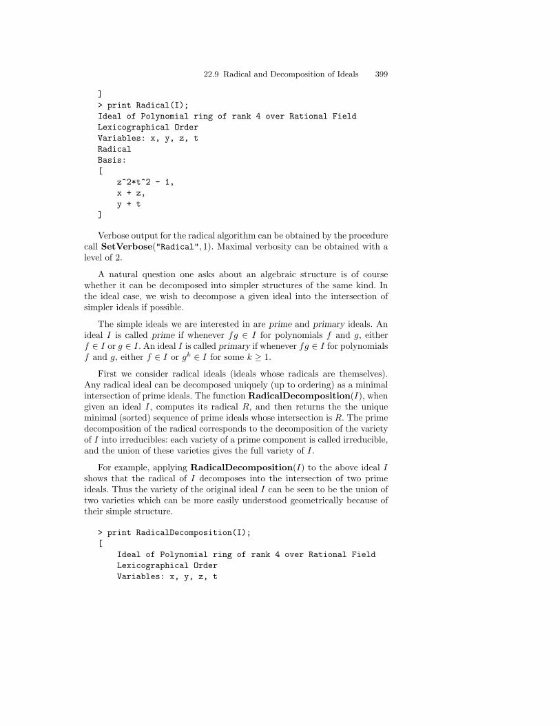
22.9 Radical and Decomposition of Ideals 399
]> print Radical(I);Ideal of Polynomial ring of rank 4 over Rational FieldLexicographical OrderVariables: x, y, z, tRadicalBasis:[
z^2*t^2 - 1,x + z,y + t
]
Verbose output for the radical algorithm can be obtained by the procedurecall SetVerbose("Radical", 1). Maximal verbosity can be obtained with alevel of 2.
A natural question one asks about an algebraic structure is of coursewhether it can be decomposed into simpler structures of the same kind. Inthe ideal case, we wish to decompose a given ideal into the intersection ofsimpler ideals if possible.
The simple ideals we are interested in are prime and primary ideals. Anideal I is called prime if whenever fg ∈ I for polynomials f and g, eitherf ∈ I or g ∈ I. An ideal I is called primary if whenever fg ∈ I for polynomialsf and g, either f ∈ I or gk ∈ I for some k ≥ 1.
First we consider radical ideals (ideals whose radicals are themselves).Any radical ideal can be decomposed uniquely (up to ordering) as a minimalintersection of prime ideals. The function RadicalDecomposition(I), whengiven an ideal I, computes its radical R, and then returns the the uniqueminimal (sorted) sequence of prime ideals whose intersection is R. The primedecomposition of the radical corresponds to the decomposition of the varietyof I into irreducibles: each variety of a prime component is called irreducible,and the union of these varieties gives the full variety of I.
For example, applying RadicalDecomposition(I) to the above ideal Ishows that the radical of I decomposes into the intersection of two primeideals. Thus the variety of the original ideal I can be seen to be the union oftwo varieties which can be more easily understood geometrically because oftheir simple structure.
> print RadicalDecomposition(I);[
Ideal of Polynomial ring of rank 4 over Rational FieldLexicographical OrderVariables: x, y, z, t

400 22. Multivariate Polynomial Rings
Dimension 1, Radical, PrimeGroebner basis:[
x + z,y + t,z*t + 1
],Ideal of Polynomial ring of rank 4 over Rational FieldLexicographical OrderVariables: x, y, z, tDimension 1, Radical, PrimeGroebner basis:[
x + z,y + t,z*t - 1
]]
A general ideal I does not necessarily decompose into the intersectionof prime ideals. That is why the notion of a primary ideal is necessary.It turns out that an ideal I can be decomposed into an intersection ofprimary ideals. For each primary ideal J of the decomposition, its radi-cal is a prime ideal and is called the associated prime of J . The functionPrimaryDecomposition(I) returns a primary decomposition of the givenideal, together with the associated primes.
Thus, continuing the above example, a primary decomposition of I hassize 8. Notice that the sequence of associated primes (P ) contains idealswhich contain other ideals of the associated primes. This phenomenon doesnot occur for radical ideals so it shows the more subtle complications thatcan arise with non-radical ideals.
> Q, P := PrimaryDecomposition(I);> print #Q, #P;8 8> print [Basis(J): J in Q];[
[ x + z, y + t, z*t + 1 ],[ x + z, y + t, z*t - 1 ],[ x + y + 2, y^2 + 2*y + 1, z - 1, t - 1 ],[ x + y - 2, y^2 - 2*y + 1, z + 1, t + 1 ],[ x + 1, y + z - 2, z^2 - 2*z + 1, t + 1 ],[ x - 1, y + z + 2, z^2 + 2*z + 1, t - 1 ],[ x + y + 2*t, y^2 + 2*y*t - 1, z - t, t^2 + 1 ],
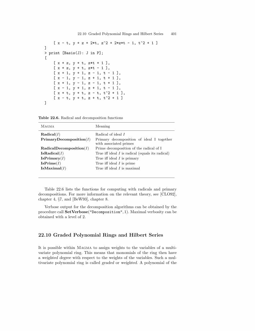
22.10 Graded Polynomial Rings and Hilbert Series 401
[ x - t, y + z + 2*t, z^2 + 2*z*t - 1, t^2 + 1 ]]> print [Basis(J): J in P];[
[ x + z, y + t, z*t + 1 ],[ x + z, y + t, z*t - 1 ],[ x + 1, y + 1, z - 1, t - 1 ],[ x - 1, y - 1, z + 1, t + 1 ],[ x + 1, y - 1, z - 1, t + 1 ],[ x - 1, y + 1, z + 1, t - 1 ],[ x + t, y + t, z - t, t^2 + 1 ],[ x - t, y + t, z + t, t^2 + 1 ]
]
Table 22.6. Radical and decomposition functions
Magma Meaning
Radical(I) Radical of ideal I
PrimaryDecomposition(I) Primary decomposition of ideal I togetherwith associated primes
RadicalDecomposition(I) Prime decomposition of the radical of I
IsRadical(I) True iff ideal I is radical (equals its radical)
IsPrimary(I) True iff ideal I is primary
IsPrime(I) True iff ideal I is prime
IsMaximal(I) True iff ideal I is maximal
Table 22.6 lists the functions for computing with radicals and primarydecompositions. For more information on the relevant theory, see [CLO92],chapter 4, §7, and [BeW93], chapter 8.
Verbose output for the decomposition algorithms can be obtained by theprocedure call SetVerbose("Decomposition", 1). Maximal verbosity can beobtained with a level of 2.
22.10 Graded Polynomial Rings and Hilbert Series
It is possible within Magma to assign weights to the variables of a multi-variate polynomial ring. This means that monomials of the ring then havea weighted degree with respect to the weights of the variables. Such a mul-tivariate polynomial ring is called graded or weighted. A polynomial of the

402 22. Multivariate Polynomial Rings
ring whose monomials all have the same weighted degree is called homoge-neous. The polynomial ring can be decomposed as the direct sum of gradedhomogeneous components.
Suppose a polynomial ring P has n variables x1, . . . , xn and the weights forthe variables are d1, . . . , dn respectively. Then for a monomial m = xe1
1 · · ·xenn
of P (with ei ≥ 0 for 1 ≤ i ≤ n), the weighted degree of m is defined to be∑ni=1 eidi.
To create a polynomial ring P = R[x1, . . . , xn] with weights d1, . . . , dn
corresponding respectively to the variables, one simply uses the functionPolynomialRing(R,Q), where Q is the sequence [d1, . . . , dn] of weights cor-responding to the variables. The rank n of the polynomial ring is determinedby the length of the sequence Q.
For example:
> P<x, y, z> := PolynomialRing(RationalField(), [1, 2, 4]);> print P;Graded Polynomial ring of rank 3 over Rational FieldLexicographical OrderVariables: x, y, zVariable weights: 1 2 4
A polynomial ring constructed in the usual way without given weights isassumed to have weight 1 for each variable.
The function WeightedDegree(f) returns the weighted degree of thepolynomial f (the maximum of the weighted degrees of the monomials off), while the function LeadingWeightedDegree(f) returns the weighteddegree of the leading monomial of f .
Continuing the above example:
> P<x, y, z> := PolynomialRing(RationalField(), [1, 2, 4]);> print WeightedDegree(x);1> print WeightedDegree(y);2> print WeightedDegree(z);4> print WeightedDegree(x^2*y*z^3);16> print TotalDegree(x^2*y*z^3);6

22.10 Graded Polynomial Rings and Hilbert Series 403
The function IsHomogeneous(f) returns whether f is homogeneouswith respect to the weights on the variables (i.e., whether the weighted de-grees of the monomials of f are all equal). Similarly, the function IsHomogeneous(I)returns whether the ideal I is homogeneous with respect to the weights onthe variables of the polynomial ring of which it is an ideal—this is equivalentto whether I possesses a basis consisting of homogeneous polynomials alone.
Continuing the above example:
> P<x, y, z> := PolynomialRing(RationalField(), [1, 2, 4]);> print IsHomogeneous(x);true> print IsHomogeneous(x + y);false> print IsHomogeneous(x^2 + y);true> I := ideal<P | y^2 + 2*x^2*y, (x^4 + z)^2, x + y, x^2 + x>;> print IsHomogeneous(I);true
For a homogeneous ideal I of the graded polynomial ring P = K[x1, . . . , xn],the quotient ring P/I is a graded vector space in the following way: P/I isthe direct sum of the vector spaces Vd for d = 0, 1, . . . where Vd is the K-vector space consisting of all homogeneous polynomials in P/I (i.e., reducedresidues of polynomials of P with respect to I) of weighted degree d. TheHilbert Series of the graded vector space P/I is the generating function
HP/I(t) =∞∑
d=0
dim(Vd)td.
The Hilbert series can be written as a rational function in the indeterminatet.
The function HilbertSeries(I) returns the Hilbert Series HP/I of P/I,where I is a homogeneous ideal of the (possibly graded) polynomial ring P ,as an element of the univariate function field over the ring of integers. Forexample:
> P<x, y, z> := PolynomialRing(RationalField(), [1, 2, 4]);> I := ideal<P | x, y^2, z^3>;> H<t> := HilbertSeries(I);> print H;-1/(t^2 - 1)
If the weights on the variables of P are all 1, then there exists the Hilbertpolynomial FP/I(d) corresponding to the Hilbert series HP/I(t) which is a

404 22. Multivariate Polynomial Rings
univariate polynomial in Q[d] such that FP/I(i) is equal to the coefficient ofti in the Hilbert series for all i ≥ k for some fixed k.
The function HilbertPolynomial(I) returns the Hilbert polynomialFP/I corresponding to HP/I , where I is a homogeneous ideal of the (pos-sibly graded) polynomial ring P , as an element of the univariate polynomialring over the rational field. The function also returns the index of regularityk which is the minimal integer k ≥ 0 such that FP/I(i) equals the coefficientof ti in the Hilbert series for all i ≥ k. For example:
> P<x, y, z> := PolynomialRing(RationalField(), 3);> I := ideal<P | x^3 + x^2*y + x^2*z, x*y^2 + y^3 + y^2*z>;> H<t> := HilbertSeries(I);> print H;(-t^4 - t^3 + t^2 + t + 1)/(t^2 - 2*t + 1)> F<d>, k := HilbertPolynomial(I);> print F;d + 5> print k;3> // Check that evaluations of F for d >= 3 match coefficients of H:> SR<u> := PowerSeriesRing(IntegerRing());> print SR ! H;1 + 3*u + 6*u^2 + 8*u^3 + 9*u^4 + 10*u^5 + 11*u^6 + 12*u^7 +
13*u^8 + 14*u^9 + 15*u^10 + 16*u^11 + 17*u^12 + 18*u^13+ 19*u^14 + 20*u^15 + 21*u^16 + 22*u^17 + 23*u^18 +24*u^19 + O(u^20)
> print Evaluate(F, 3);8> print Evaluate(F, 4);9
22.11 Dimension of Ideals
Let I be an ideal of the polynomial ring P = K[x1, . . . , xn]. Let X be theset x1, . . . , xn of variables of P . A subset U of X is called independentmodulo I if I ∩K[U ] = ∅. A subset U of X is called maximally independentmodulo I if U is independent modulo I, and no proper superset of U isindependent modulo I. The dimension of I is defined to be the maximum ofthe cardinalities of all the independent sets modulo I. Note that dimension0 according to this definition does correspond to the definition of a zero-dimensional ideal given above.

22.11 Dimension of Ideals 405
The Magma function Dimension(I) computes the dimension d of theideal I. The function also returns a (sorted) sequence U of integers of lengthd such that the variables of P corresponding to the integers of U constitutea maximally independent set modulo I.
For example, the following ideal has dimension 1 obviously, since thevariable z is ‘free’ so a maximally independent set for the ideal is z.
> P<x, y, z> := PolynomialRing(RationalField(), 3);> I := ideal<P | x, y^2>;> print Dimension(I);1 [ 3 ]


23. Power Series and Laurent Series
This chapter explains the operations on power series rings and Laurent seriesrings in Magma. These structures share many operations with polynomialrings R[x], and that there are some similarities with the real and complexfields with regard to the control of precision.
23.1 Power Series and Laurent Series
Power series rings R[[x]] and Laurent series rings R((x)) over a commutativering R contain polynomial-like elements which are, loosely speaking, poly-nomials with an infinite number of terms. More strictly, a power series isan element of the form avxv + av+1x
v+1 + av+2xv+2 + · · · , where v is a
non-negative integer and av 6= 0 (unless the series is zero). Here the ai areelements of R, and x is the indeterminate. The other concept, Laurent series,is slightly more general: a Laurent series is permitted to have a finite numberof negative powers of x as well, so v may be a negative integer. One way oflooking at a Laurent series is to consider it as a power series multiplied byxk, for some k ∈ ZZ.
Since computer memory is finite, power series and Laurent series inMagma with an infinite number of non-zero terms must be stored in a trun-cated form. Thus the infinite series above is stored as avxv + av+1x
v+1 +av+2x
v+2 + · · ·+ ap−1xp−1 + O(xp), for some integer p. The notation O(xp),
known colloquially as ‘big-oh’ notation, denotes unknown terms in which theexponent of x is at least p.
Table 23.1 (p. 408) lists some functions on power series and infinite series.Given the series f = avxv+av+1x
v+1+av+2xv+2+· · ·+ap−1x
p−1+O(xp), thenumber v is called the valuation of f , and is the least power of x occurringwith a non-zero coefficient in f . As noted above, v may be any integer ina Laurent series, but must be non-negative in a power series. The numberp is called the absolute precision, and p − v is called the relative precision.The relationship between these two kinds of precision is that the relativeprecision of f equals the absolute precision of f
xv . The degree is the highest-
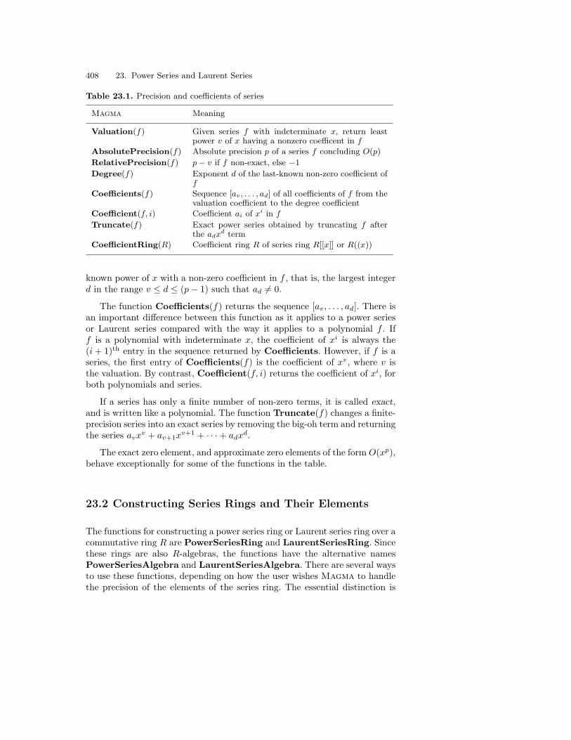
408 23. Power Series and Laurent Series
Table 23.1. Precision and coefficients of series
Magma Meaning
Valuation(f) Given series f with indeterminate x, return leastpower v of x having a nonzero coefficent in f
AbsolutePrecision(f) Absolute precision p of a series f concluding O(p)
RelativePrecision(f) p− v if f non-exact, else −1
Degree(f) Exponent d of the last-known non-zero coefficient off
Coefficients(f) Sequence [av, . . . , ad] of all coefficients of f from thevaluation coefficient to the degree coefficient
Coefficient(f, i) Coefficient ai of xi in f
Truncate(f) Exact power series obtained by truncating f afterthe adxd term
CoefficientRing(R) Coefficient ring R of series ring R[[x]] or R((x))
known power of x with a non-zero coefficient in f , that is, the largest integerd in the range v ≤ d ≤ (p− 1) such that ad 6= 0.
The function Coefficients(f) returns the sequence [av, . . . , ad]. There isan important difference between this function as it applies to a power seriesor Laurent series compared with the way it applies to a polynomial f . Iff is a polynomial with indeterminate x, the coefficient of xi is always the(i + 1)th entry in the sequence returned by Coefficients. However, if f is aseries, the first entry of Coefficients(f) is the coefficient of xv, where v isthe valuation. By contrast, Coefficient(f, i) returns the coefficient of xi, forboth polynomials and series.
If a series has only a finite number of non-zero terms, it is called exact,and is written like a polynomial. The function Truncate(f) changes a finite-precision series into an exact series by removing the big-oh term and returningthe series avxv + av+1x
v+1 + · · ·+ adxd.
The exact zero element, and approximate zero elements of the form O(xp),behave exceptionally for some of the functions in the table.
23.2 Constructing Series Rings and Their Elements
The functions for constructing a power series ring or Laurent series ring over acommutative ring R are PowerSeriesRing and LaurentSeriesRing. Sincethese rings are also R-algebras, the functions have the alternative namesPowerSeriesAlgebra and LaurentSeriesAlgebra. There are several waysto use these functions, depending on how the user wishes Magma to handlethe precision of the elements of the series ring. The essential distinction is

23.2 Constructing Series Rings and Their Elements 409
between free rings, in which each element has its own precision, and fixed orlimited precision rings, in which every element has a precision less than orequal to some fixed number.
23.2.1 Free Precision Series Rings
The method for creating a free precision power series ring is to give thefunction PowerSeriesRing a single argument, the coefficient ring R. Forexample:
> Q := RationalField();> P<x> := PowerSeriesRing(Q);> print P;Power Series Algebra in x over Rational Field
Exact elements of P may be created like polynomials:
> p1 := 6*x^5 + 3/5*x^17 - 4*x^144; print p1;6*x^5 + 3/5*x^17 - 4*x^144> print Valuation(p1), Degree(p1);5 144
To create an element with a finite absolute precision p, type O(x^p) as oneof the terms:
> p2 := 5*x^18 - 7*x^22 + 10*x^23 + O(x^47);> print p2;5*x^18 - 7*x^22 + 10*x^23 + O(x^47)> print Valuation(p2), Degree(p2);18 23> print AbsolutePrecision(p2), RelativePrecision(p2);47 29> print Truncate(p2);5*x^18 - 7*x^22 + 10*x^23
The sequence of coefficients of a series begins at the valuation coefficientand ends at the degree coefficient. For instance:
> print Coefficients(p2);[ 5, 0, 0, 0, -7, 10 ]
This kind of coefficient sequence can also be used in the opposite direction,to create a series by means of the elt constructor:

410 23. Power Series and Laurent Series
elt< P | v, Q, r >
It creates the element with valuation v, coefficient sequence Q and relativeprecision r in the power series ring or Laurent series ring P . The value of rmust be positive or −1. If v is omitted, then the valuation is set to be zero,and if r is omitted, then the relative precision is set to be the length of Q.For instance, the following element is equal to p2 :
> print elt< P | 18, [ 5, 0, 0, 0, -7, 10 ], 29 >;5*x^18 - 7*x^22 + 10*x^23 + O(x^47)
To create an exact series, type −1 for r:
> print elt< P | [4..40 by 3], -1 >;4 + 7*x + 10*x^2 + 13*x^3 + 16*x^4 + 19*x^5 + 22*x^6
+ 25*x^7 + 28*x^8 + 31*x^9 + 34*x^10 + 37*x^11 + 40*x^12
A final way to create elements is to coerce an element of the coefficientring, or a sequence of such elements, into the series ring P . The coercion ofa single element gives an exact result. However, the coercion of a sequence Qgives the same result as elt< P | Q >, since it is assumed that the valuationis zero and that the final entry of Q is the last-known term. For instance:
> print P![4, 34, 59, 0, 2, 0];4 + 34*x + 59*x^2 + 2*x^4 + O(x^6)
Elements of Laurent series rings may be created according to the samemethods as for power series rings, except that negative powers of the inde-terminate are allowed:
> L<y> := LaurentSeriesRing(Q);> print 5*y^-2 + 16*y^5 + O(y^7);5*y^-2 + 16*y^5 + O(y^7)> print elt< L | -19, [4,24,0,3,5], 21 >;4*y^-19 + 24*y^-18 + 3*y^-16 + 5*y^-15 + O(y^2)> print elt< L | -90, [7,3,4], 75 >;7*y^-90 + 3*y^-89 + 4*y^-88 + O(y^-15)
In some circumstances, a non-exact power series or Laurent series is cal-culated without a particular relative precision being requested. For instance,the inverse of a series generally has an infinite number of non-zero terms:
> p3 := (2 + p1) ^ -1;> print p3;1/2 - 3/2*x^5 + 9/2*x^10 - 27/2*x^15 - 3/20*x^17 + O(x^20)

23.2 Constructing Series Rings and Their Elements 411
It is impossible to return an infinite series, so Magma must know whatprecision to use. This default relative precision is stored in the "Precision"attribute of the ring. To find the current value of the precision attributefor the free series ring P , use the function HasAttribute(P, "Precision"),which returns two values. The second return value is the current value ofthe precision attribute. (The first return value is always true in this case,because the precision attribute is always defined for any free series ring thathas been created.) For instance:
> print HasAttribute(P, "Precision");true 20
Therefore the attribute’s value is 20. This number 20 has been chosen by thedesigners of Magma as the default value of the precision attribute for freeseries rings.
There are two ways to make the precision attribute of a free series ringdifferent from 20. It may either be changed once the ring has been created, orit may be given a non-default value at the same time as the ring is created.The procedure AssertAttribute(P, "Precision", p): may be used to changethe precision attribute of an existing ring P to p:
> AssertAttribute(P, "Precision", 28);> print (2 + p1) ^ -1;1/2 - 3/2*x^5 + 9/2*x^10 - 27/2*x^15 - 3/20*x^17 + 81/2*x^20
+ 9/10*x^22 - 243/2*x^25 - 81/20*x^27 + O(x^28)> print p3;1/2 - 3/2*x^5 + 9/2*x^10 - 27/2*x^15 - 3/20*x^17 + O(x^20)
Notice that the change in the attribute only affects newly-created elements,not pre-existing ones such as p3 . On the other hand, to create a free seriesring with a precision attribute other than 20, assign a value to the parameterPrecision when calling PowerSeriesRing(R) or LaurentSeriesRing(R):
> Pb<xb> := PowerSeriesRing(Q: Precision := 8);> Lb<yb> := LaurentSeriesRing(Q: Precision := 8);
When the ring has been created in this way, the default relative precision willbe 8:
> print xb^3 / (1 - xb);xb^3 + xb^4 + xb^5 + xb^6 + xb^7 + xb^8 + xb^9
+ xb^10 + O(xb^11)> print yb^3 / (1 - yb);yb^3 + yb^4 + yb^5 + yb^6 + yb^7 + yb^8 + yb^9
+ yb^10 + O(yb^11)

412 23. Power Series and Laurent Series
23.2.2 Fixed Absolute Precision Power Series Rings
A different approach to the precision issue for power series rings should beused in cases where all the elements of the ring are to have the same precision,with no exceptions. The function for creating a fixed absolute precision powerseries ring, is PowerSeriesRing(R, p):
> P30<s> := PowerSeriesRing(Q, 30);> print P30;Power Series Algebra of precision 30 in sover Rational Field> print Precision(P30);30
Note that the function Precision returns p. This integer will be the absoluteprecision of all elements of the power series ring. For example:
> print s^5;s^5 + O(s^30)> print P30!0;O(s^30)
A power series ring of fixed absolute precision p over R may be consideredmathematically as the quotient structure R[[x]]/xp. That is, all elements ofR[[x]] with the same coefficients from x0 to xp−1 are considered to form anequivalence class.
Since every element of a fixed precision power series ring has the sameabsolute precision, and there are no exact elements, the creation of elementsis slightly easier. They may be entered like polynomials, as shown above.Alternatively, the notation elt< P | v, Q > will produce the element withvaluation v and coefficient sequence Q, or simply P !Q if the valuation iszero. Although Magma will accept both the O function and the r option inthe elt constructor, without giving an error message, it will ignore the givenvalues.
23.2.3 Limited Relative Precision Laurent Series Rings
The final kind of series ring is a limited relative precision Laurent series ring.It is created by the function LaurentSeriesRing(R, p):
> L30<t> := LaurentSeriesRing(Q, 30);> print L30;Laurent Series Algebra of precision 30 in t

23.3 Operations on Series 413
over Rational Field> print Precision(L30);30
All elements of this ring will have relative precision less than or equal to p.(This integer is returned by the function Precision.) For example:
> print t^5;t^5 + O(t^35)> print t^5 + O(t^12);t^5 + O(t^12)> print L30!0;0
Observe that if an element is typed as a polynomial, then it is given therelative precision p. The O function should be used for creating elementswith relative precision less than p.
23.3 Operations on Series
Arithmetic on power series or Laurent series is performed with the usualoperators, but the user should be aware of how the precision of the resultis calculated. In fixed precision power series rings, the absolute precision ofevery element is the same, so there is no problem. In the other three kinds ofseries rings, the absolute precision of f + g is the minimum of the absoluteprecisions of f and g, and the relative precision of f*g is the minimum of therelative precisions of f and g.
The operator / performs division. For example:
> print x^5 / (x^2 + x^3);x^3 - x^4 + x^5 - x^6 + x^7 - x^8 + x^9 - x^10 + x^11
- x^12 + x^13 - x^14 + x^15 - x^16 + x^17 - x^18+ x^19 - x^20 + x^21 - x^22 + O(x^23)
To evaluate the expression f/g, Magma divides f and g by the valuation of gto obtain f ′/g′, and then returns f ′*g′−1. Therefore, in order for the divisionto succeed, the constant term of g′ (and hence the ‘valuation coefficient’ of g)must be a unit. It follows that if the coefficient ring R is not a field, divisionis not generally available. Of course, if f and g are power series rather thanLaurent series, it is also required that the valuation of the result be non-negative.
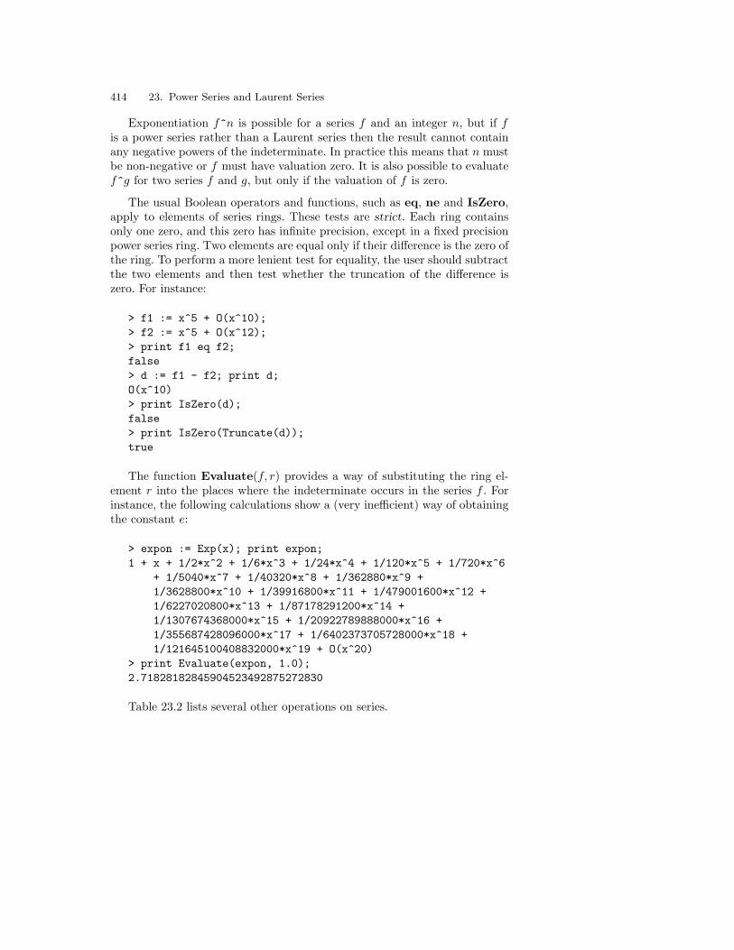
414 23. Power Series and Laurent Series
Exponentiation f^n is possible for a series f and an integer n, but if fis a power series rather than a Laurent series then the result cannot containany negative powers of the indeterminate. In practice this means that n mustbe non-negative or f must have valuation zero. It is also possible to evaluatef^g for two series f and g, but only if the valuation of f is zero.
The usual Boolean operators and functions, such as eq, ne and IsZero,apply to elements of series rings. These tests are strict. Each ring containsonly one zero, and this zero has infinite precision, except in a fixed precisionpower series ring. Two elements are equal only if their difference is the zero ofthe ring. To perform a more lenient test for equality, the user should subtractthe two elements and then test whether the truncation of the difference iszero. For instance:
> f1 := x^5 + O(x^10);> f2 := x^5 + O(x^12);> print f1 eq f2;false> d := f1 - f2; print d;O(x^10)> print IsZero(d);false> print IsZero(Truncate(d));true
The function Evaluate(f, r) provides a way of substituting the ring el-ement r into the places where the indeterminate occurs in the series f . Forinstance, the following calculations show a (very inefficient) way of obtainingthe constant e:
> expon := Exp(x); print expon;1 + x + 1/2*x^2 + 1/6*x^3 + 1/24*x^4 + 1/120*x^5 + 1/720*x^6
+ 1/5040*x^7 + 1/40320*x^8 + 1/362880*x^9 +1/3628800*x^10 + 1/39916800*x^11 + 1/479001600*x^12 +1/6227020800*x^13 + 1/87178291200*x^14 +1/1307674368000*x^15 + 1/20922789888000*x^16 +1/355687428096000*x^17 + 1/6402373705728000*x^18 +1/121645100408832000*x^19 + O(x^20)
> print Evaluate(expon, 1.0);2.71828182845904523492875272830
Table 23.2 lists several other operations on series.
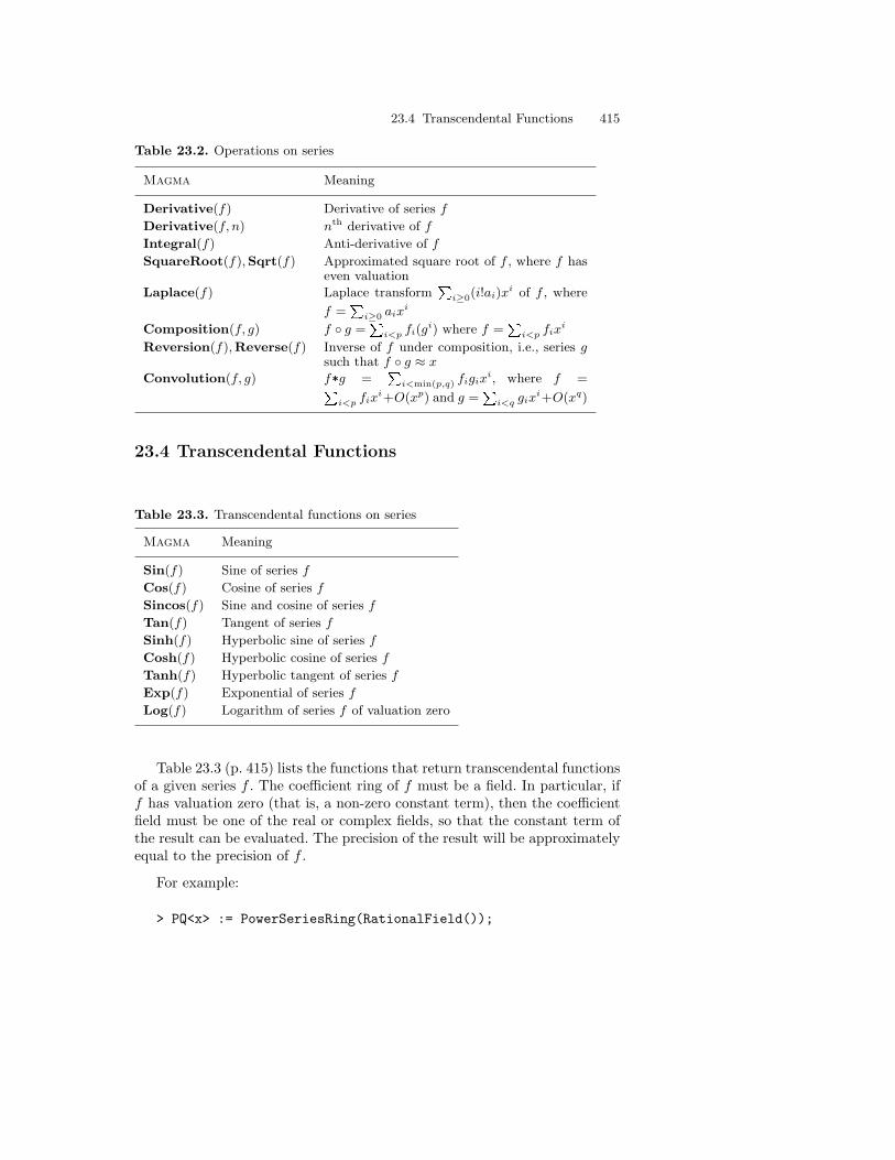
23.4 Transcendental Functions 415
Table 23.2. Operations on series
Magma Meaning
Derivative(f) Derivative of series f
Derivative(f, n) nth derivative of f
Integral(f) Anti-derivative of f
SquareRoot(f),Sqrt(f) Approximated square root of f , where f haseven valuation
Laplace(f) Laplace transformP
i≥0(i!ai)xi of f , where
f =P
i≥0 aixi
Composition(f, g) f g =P
i<p fi(gi) where f =
Pi<p fix
i
Reversion(f),Reverse(f) Inverse of f under composition, i.e., series gsuch that f g ≈ x
Convolution(f, g) f*g =P
i<min(p,q) figixi, where f =P
i<p fixi+O(xp) and g =
Pi<q gix
i+O(xq)
23.4 Transcendental Functions
Table 23.3. Transcendental functions on series
Magma Meaning
Sin(f) Sine of series f
Cos(f) Cosine of series f
Sincos(f) Sine and cosine of series f
Tan(f) Tangent of series f
Sinh(f) Hyperbolic sine of series f
Cosh(f) Hyperbolic cosine of series f
Tanh(f) Hyperbolic tangent of series f
Exp(f) Exponential of series f
Log(f) Logarithm of series f of valuation zero
Table 23.3 (p. 415) lists the functions that return transcendental functionsof a given series f . The coefficient ring of f must be a field. In particular, iff has valuation zero (that is, a non-zero constant term), then the coefficientfield must be one of the real or complex fields, so that the constant term ofthe result can be evaluated. The precision of the result will be approximatelyequal to the precision of f .
For example:
> PQ<x> := PowerSeriesRing(RationalField());

416 23. Power Series and Laurent Series
> print Sincos(x);x - 1/6*x^3 + 1/120*x^5 - 1/5040*x^7 + 1/362880*x^9 -
1/39916800*x^11 + 1/6227020800*x^13 -1/1307674368000*x^15 + 1/355687428096000*x^17 -1/121645100408832000*x^19 + O(x^21)
1 - 1/2*x^2 + 1/24*x^4 - 1/720*x^6 + 1/40320*x^8 -1/3628800*x^10 + 1/479001600*x^12 - 1/87178291200*x^14 +1/20922789888000*x^16 - 1/6402373705728000*x^18 +O(x^20)
> print Exp(x + O(x^15));1 + x + 1/2*x^2 + 1/6*x^3 + 1/24*x^4 + 1/120*x^5 + 1/720*x^6
+ 1/5040*x^7 + 1/40320*x^8 + 1/362880*x^9 +1/3628800*x^10 + 1/39916800*x^11 + 1/479001600*x^12 +1/6227020800*x^13 + 1/87178291200*x^14 + O(x^15)
> P30R<y> := PowerSeriesRing(RealField(), 30);> print Log(1 + y);y - 1/2*y^2 + 1/3*y^3 - 1/4*y^4 + 1/5*y^5 - 1/6*y^6 +
1/7*y^7 - 1/8*y^8 + 1/9*y^9 - 1/10*y^10 + 1/11*y^11 -1/12*y^12 + 1/13*y^13 - 1/14*y^14 + 1/15*y^15 -1/16*y^16 + 1/17*y^17 - 1/18*y^18 + 1/19*y^19 -1/20*y^20 + 1/21*y^21 - 1/22*y^22 + 1/23*y^23 -1/24*y^24 + 1/25*y^25 - 1/26*y^26 + 1/27*y^27 -1/28*y^28 + 1/29*y^29 + O(y^30)
These series may also be used to check identities, although the results maynot be exact when floating point arithmetic is used:
> print Derivative(Tan(x)) eq Cos(x)^-2;true> C<i> := ComplexField();> PC<z> := PowerSeriesRing(C);> print Exp(i*z) eq (Cos(z) + i*Sin(z));true> R8 := RealField(8);> PR8<t> := PowerSeriesRing(R8);> print Sin(Pi(R8)/2 - t) - Cos(t);-0.00000001 + 3.673205e-6*y - 6.12201e-7*y^3 + 3.061e-8*y^5
- 7.288006e-10*y^7 + 1.1222e-11*y^9 - 9.22113e-14*y^11 +5.8988e-16*y^13 - 2.88949e-18*y^15 + 1.0327e-20*y^17 -3.1957e-23*y^19 + O(y^20)

23.5 Series as Generating Functions 417
23.5 Series as Generating Functions
One of the applications of series is in counting theory. A generating functionis a series that carries in its coefficients the values of some function τ whosedomain is the integers (or just the non-negative integers, for a power series).The nth coefficient is the function value τ(n).
For example, the sequence of Catalan numbers arises in several combina-torial contexts. The nth Catalan number is the number of balanced arrange-ments of n left brackets and n right brackets, that is, arrangements such as(()((((())))((())))) in which all n pairs of brackets are nested legally. It canbe shown that
C(x) =1−√1− 4x
2x
is a closed form generating function for the Catalan numbers. The followinglines construct this power series and print its coefficents:
> PQ<x> := PowerSeriesRing(RationalField());> C := (1 - Sqrt(1-4*x)) / (2*x);> print Coefficients(C);[ 1, 1, 2, 5, 14, 42, 132, 429, 1430, 4862, 16796, 58786,208012, 742900, 2674440, 9694845, 35357670, 129644790,477638700 ]
It can also be shown that the nth Catalan number is equal to 1n+1
(2nn
). The
following lines show that the results from the generating function and thisidentity are equal in the case n = 7:
> print Coefficient(C, 7);429> print Binomial(2*7, 7) div (7+1); // division is exact429
The example below is a verification (within the precision) of the identityC − 1 = xC2. It shows that the difference between the two sides of theequation is an approximation to zero:
> D := x*C^2 - (C - 1);> print D;O(x^19)> print IsZero(Truncate(D));true


24. Finite Fields
A finite field or Galois field is a field containing only a finite number ofelements q. Such a field exists only if q equals pn, a positive power of a primenumber p and, up to isomorphism, there is exactly one field for each such q.The numbers p and n for a field of size pn are called the characteristic andthe degree. A finite field of pn elements contains a subfield of cardinality pm
when m divides n. In particular, any finite field contains a subfield of primecardinality p; such a field is called a prime field
In Magma it is well possible to work in a finite field created from thespecification of pn only. The first section of this Chapter provides the details.In many situations, however, it is convenient to have more control over therepresentation of elements of finite fields and of the relations between finitefields. Later sections of this Chapter contain the more advanced mechanismin Magma for dealing with that.
24.1 Finite Fields by Cardinality
24.1.1 Constructing Finite Fields
The simplest way of creating the Galois field with q elements in Magma isto use the function FiniteField (with which GaloisField is synonymous,allowing the abbreviation GF). The function may be used as GF(q) or asGF(p, n), with exactly the same result except that in the second versionMagma does not have the extra task of factorizing q; this may save sometime if p is large.
> F32 := GF(2, 5); print F32;Finite field of size 2^5> print F32 eq GF(32);true

420 24. Finite Fields
Given a finite field F with pn elements, the Magma functions Degree(F )and Characteristic(F ) return p and n. The cardinality q = pn of F isreturned by #F .
Once a finite field of cardinality pn has been created, it is possible todefine extensions and subfields by use of ext and sub, specifying just thedesired degree. For extensions any degree is allowed, for subfields the degreemust divide n of course.
> G := GF(11, 3);> H := ext< G | 4 >;> I := sub< H | 6 >;> print I;Finite field of size 11^6
There exist many more sophisticated ways of creating extensions and sub-fields, which we will encounter below.
Arithmetic in a prime field of cardinality p is just arithmetic modulo p. Itis possible to do such arithmetic without creating the finite field, with integeroperations (see ??).
To define elements in larger fields we use some distinguished element, agenerator. Any finite field F in Magma is built up as the extension of anotherfinite field G (called the ground field) by an element called the generator ofthe field. The ground field is either explicit in the construction, for examplewhen we use ext, or implicit, such as in the sub construction and in theGF(p, n) definition. In such implicit cases the ground field is the smallestsubfield, i.e., the prime subfield.
Any prime field will be its own ground field, with generator simply 1.There are functions for retrieving the ground field and prime subfield.
> G := GF(11, 3);> H := ext< G | 4 >;> print PrimeField(G), PrimeField(H);Finite field of size 11Finite field of size 11> print GroundField(G), GroundField(H);Finite field of size 11Finite field of size 11^3
24.1.2 Creation of Elements
The generator of a finite field F has the property that every other elementof the field can be written as a polynomial expression in this generator, with

24.1 Finite Fields by Cardinality 421
coefficients from the ground field G. This polynomial representation is uniqueif we allow polynomials of degree less than n −m only, where n and m arethe degrees of F and G.
The generator can be extracted from the field using Generator(G) orG.1. but it is much better to assign it to a variable and at the same timedetermine the way in which elements of the field will be printed by the familiarangle bracket construction on the left-hand side in the definition of the finitefield:
> G<g> := GF(11, 3);> print G.1;g> print Random(G);g^29> print g^2-g+10;g^1158
As can be seen here, the elements of this finite field are not printed as apolynomial of degree less than 3 in the generator g. The reason is that thereis another representation of elements that is often convenient. The non-zeroelements of a finite field form a finite (multiplicative) group that is cyclic oforder q − 1. Once a generator v of this group is found, every element of thefield except zero can be written uniquely as vk with 0 ≤ k < q − 1. We willcall this the power presentation. An element of the field that generates themultiplicative group is called primitive.
In principle we then have two representations for non-zero elements inany finite field: the polynomial presentation and the power presentation. Forsmall fields (for q less than around 106) both may be used; by default elementsare given in the power presentation, but by changing an attribute on the fieldit is possible to change this. Continuing the previous example:
> AssertAttribute(G, "PowerPrinting", false);> print g^29, g^1158;g^2 + 9*g + 10g^2 + 10*g + 10
For large fields elements will always be shown in polynomial representation.The reason is that it is not always easy to find a primitive polynomial, andit may be hard to convert between polynomial and power presentations. Ingeneral it is not guaranteed that field generators are primitive. The functionIsPrimitive may be used to check primitivity of an element. Moreover, withPrimitiveElement(F ) a primitive element can be found.
> H<h> := ext< G | 4>;

422 24. Finite Fields
> print Random(H);> print IsPrimitive(h);true> print IsPrimitive(h+1);false> print FactoredOrder(h+1);[ <2, 4>, <3, 2>, <5, 1>, <13, 1>, <19, 1>, <37, 1>, <61, 1>, <1117, 1> ]> print FactoredOrder(h);[ <2, 4>, <3, 2>, <5, 1>, <7, 1>, <13, 1>, <19, 1>, <37, 1>, <61, 1>, <1117, 1> ]> print IsPrimitive(Root(h+1, 7));true
In the above example the element h is primitive, but h + 1 is not. In facth + 1 is the 7-th power of a primitive element.
24.2 Finding Special Elements
We have seen already how to find random elements (in the example above),primitive elements, and a generator for a field over its ground field. Thefunction Generator can also be used to produce a generator over a subfieldS other than the prime field; in that case Generator(F, S) should be used.
Two more elements of a special kind have their own intrinsic function inMagma’s language. With NormalElement an element that generates a nor-mal basis can be found, that is, an element α such that α, αp, αp2
, . . . , αpn−1
forms a basis for F over its ground field. Again, NormalElement(G,S) canbe used to find an element generating a normal basis over an intermediatefield.
Other ways of obtaining the generator of a finite field are Generator(F )and F .1.
A primitive element of a finite field F is an element a that generates(multiplicatively) the group of the non-zero elements of F . The functionIsPrimitive(a) tests if a ∈ F is primitive. For example:
> print IsPrimitive(g), IsPrimitive(g^2);true false
Notice that in this case of this field g is not only a generator but also aprimitive element; this may be confirmed by calculating the powers of g:
> print Set(gf9); 1, g, g^2, g^3, 2, g^5, g^6, g^7, 0

24.3 Extensions of Finite Fields 423
Although the generator g of gf9 is a primitive element, it is not alwaystrue that the generator supplied by Magma for a finite field will be prim-itive. However, the generator will definitely be primitive if Magma is ableto use a Conway polynomial to define the field, because of the propertiesof these polynomials. Conway polynomials are available for reasonably smallfields. (See Section 24.6 for more information.) As for fields whose Conwaypolynomials are not known, such as the fields in the following example, theprimitivity of the generator depends on the field and on the generator thatMagma chooses:
> print IsPrimitive(Generator(GF(2, 128)));true> print IsPrimitive(Generator(GF(2, 100)));false
Given a field F , the function PrimitiveElement(F ) will return a prim-itive element of F , even if the Conway polynomial of F is not known.
24.3 Extensions of Finite Fields
24.3.1 Extensions by a Given Defining Polynomial
Every Galois field E of size pn, where n > 1, is a simple algebraic extensionof some field F of size pm, where m < n and m divides n. F is called theground field of E, and is isomorphic to a subfield of E. If F is not a primefield, that is, if m > 1, then it is in turn an extension of a smaller field withthe same characteristic p. This chain will eventually terminate at GF(p), theprime field of E. The integer d = m
n is the degree of the extension field Erelative to the ground field F , whereas n is the absolute degree of E, that is,its degree relative to the prime field.
The field E is created as a simple algebraic extension of degree d of F . Inother words, a root of an irreducible polynomial f of degree d with coefficientsin F is adjoined to F in order to create E. (For any given finite field anddegree, there always exists at least one irreducible polynomial of degree d overthe field.) In Magma, the ext constructor is used to create an extension. Oneform of this constructor is
ext< F | f >
If F is a finite field and f is an irreducible polynomial f of degree d withcoefficients in F , this creates an extension of degree d of the ground field F ,with f as its defining polynomial.
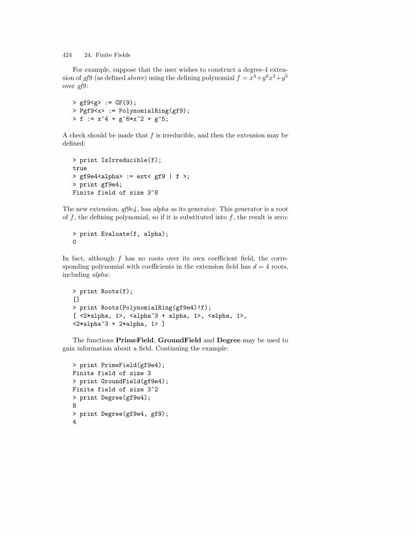
424 24. Finite Fields
For example, suppose that the user wishes to construct a degree-4 exten-sion of gf9 (as defined above) using the defining polynomial f = x4+g6x2+g5
over gf9 :
> gf9<g> := GF(9);> Pgf9<x> := PolynomialRing(gf9);> f := x^4 + g^6*x^2 + g^5;
A check should be made that f is irreducible, and then the extension may bedefined:
> print IsIrreducible(f);true> gf9e4<alpha> := ext< gf9 | f >;> print gf9e4;Finite field of size 3^8
The new extension, gf9e4 , has alpha as its generator. This generator is a rootof f , the defining polynomial, so if it is substituted into f , the result is zero:
> print Evaluate(f, alpha);0
In fact, although f has no roots over its own coefficient field, the corre-sponding polynomial with coefficients in the extension field has d = 4 roots,including alpha:
> print Roots(f);[]> print Roots(PolynomialRing(gf9e4)!f);[ <2*alpha, 1>, <alpha^3 + alpha, 1>, <alpha, 1>,<2*alpha^3 + 2*alpha, 1> ]
The functions PrimeField, GroundField and Degree may be used togain information about a field. Continuing the example:
> print PrimeField(gf9e4);Finite field of size 3> print GroundField(gf9e4);Finite field of size 3^2> print Degree(gf9e4);8> print Degree(gf9e4, gf9);4
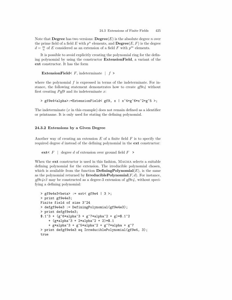
24.3 Extensions of Finite Fields 425
Note that Degree has two versions: Degree(E) is the absolute degree n overthe prime field of a field E with pn elements, and Degree(E,F ) is the degreed = m
n of E considered as an extension of a field F with pm elements.
It is possible to avoid explicitly creating the polynomial ring for the defin-ing polynomial by using the constructor ExtensionField, a variant of theext constructor. It has the form
ExtensionField< F , indeterminate | f >
where the polynomial f is expressed in terms of the indeterminate. For in-stance, the following statement demonstrates how to create gf9e4 withoutfirst creating Pgf9 and its indeterminate x:
> gf9e4<alpha>:=ExtensionField< gf9, x | x^4+g^6*x^2+g^5 >;
The indeterminate (x in this example) does not remain defined as a identifieror printname. It is only used for stating the defining polynomial.
24.3.2 Extensions by a Given Degree
Another way of creating an extension E of a finite field F is to specify therequired degree d instead of the defining polynomial in the ext constructor:
ext< F | degree d of extension over ground field F >
When the ext constructor is used in this fashion, Magma selects a suitabledefining polynomial for the extension. The irreducible polynomial chosen,which is available from the function DefiningPolynomial(E), is the sameas the polynomial returned by IrreduciblePolynomial(F, d). For instance,gf9e4e3 may be constructed as a degree-3 extension of gf9e4 , without speci-fying a defining polynomial:
> gf9e4e3<beta> := ext< gf9e4 | 3 >;> print gf9e4e3;Finite field of size 3^24> defgf9e4e3 := DefiningPolynomial(gf9e4e3);> print defgf9e4e3;$.1^3 + (g^6*alpha^3 + g^7*alpha^2 + g)*$.1^2
+ (g*alpha^3 + 2*alpha^2 + 2)*$.1+ g*alpha^3 + g^5*alpha^2 + g^7*alpha + g^7
> print defgf9e4e3 eq IrreduciblePolynomial(gf9e4, 3);true

426 24. Finite Fields
Notice from the output form of defgf9e4e3 that there is no printname forthe indeterminate in the defining polynomial, so the special symbol $.1 isemployed. If the user wishes to give the indeterminate a printname and as-sign it to an identifier, there are two methods: either the parent polynomialring may be defined, together with its indeterminate, or (more simply) anglebrackets may be used when assigning defgf9e4e3 :
> defgf9e4e3<y> := DefiningPolynomial(gf9e4e3);> print defgf9e4e3;y^3 + (g^6*alpha^3 + g^7*alpha^2 + g)*y^2 +
(g*alpha^3 + 2*alpha^2 + 2)*y +g*alpha^3 + g^5*alpha^2 + g^7*alpha + g^7
Both forms of ext, as well as ExtensionField, optionally return a secondvalue, which is the embedding monomorphism φ : F → E. This map has thesame effect as coercion of an element of F into E using the ! operator.
24.3.3 Splitting Fields
The defining polynomial for an extension formed using the ext construc-tor has to be irreducible. However, it is also possible to form an exten-sion using a non-irreducible polynomial. Given any polynomial p over F ,SplittingField(p) constructs the smallest-degree extension E of F such thatthe polynomial p factors completely into linear factors when considered as apolynomial over E.
For instance, suppose p is the polynomial defined below. The coefficientfield of p is gf9 . Over this field, p has two non-linear irreducible factors, butno roots:
> p := MinimalPolynomial(alpha^3+alpha, gf9) *> MinimalPolynomial(g*beta^2, gf9);> print Factorization(p);[
<x^4 + g^6*x^2 + g^5, 1>,<x^12 + g^3*x^11 + g^2*x^10 + g*x^8 + g^6*x^7 + g^3*x^6
+ g^2*x^5 + x^4 + 2*x^3 + g*x^2 + g^6*x + g^2, 1>]> print Roots(p);[]
Over the field gf9e4 , which contains alpha3 + alpha, p has the 4 roots corre-sponding to the degree-4 irreducible factor shown above:

24.3 Extensions of Finite Fields 427
> print Roots(PolynomialRing(gf9e4)!p);[ <2*alpha, 1>, <alpha^3 + alpha, 1>, <alpha, 1>,
<2*alpha^3 + 2*alpha, 1> ]
However, over the splitting field of p, the degree-16 polynomial p has 16 roots:
> Spl := SplittingField(p); print Spl;Finite field of size 3^24> print Roots(PolynomialRing(gf9e4e3)!p);[
<(g*alpha^3 + g^6*alpha^2 + g^3*alpha + g^5)*beta^2+ (2*alpha^3 + g^3*alpha^2 + alpha + 1)*beta+ g*alpha^3 + g^6*alpha + g^5, 1>,
<2*alpha, 1>,<(g*alpha^3 + g^2*alpha^2 + g^7*alpha + g^5)*beta^2
+ (g^3*alpha^3 + g^6*alpha^2 + g^3*alpha + 1)*beta+ alpha^3 + g^7*alpha^2 + 2*alpha + g^6, 1>,
<(2*alpha^3 + g*alpha^2 + g^7*alpha)*beta^2+ (alpha^3 + g^3*alpha + g^3)*beta+ g^3*alpha^3 + g^7*alpha^2 + g*alpha + g^2, 1>,
<2*alpha^3 + 2*alpha, 1>,<alpha, 1>,<(alpha^3 + g^5*alpha^2 + g^3*alpha + g^5)*beta^2
+ (2*alpha^3 + g^7*alpha + g^7)*beta+ g^3*alpha^3 + g*alpha^2 + g^2*alpha + 2, 1>,
<(alpha^3 + g*alpha^2 + g^7*alpha + g^2)*beta^2+ (2*alpha^3 + g^7*alpha^2 + alpha + g^2)*beta+ g^3*alpha^3 + g^6*alpha^2 + g^6*alpha + 2, 1>,
<(g^6*alpha^3 + g^3*alpha^2 + 2*alpha + g^7)*beta^2+ (g^6*alpha^3 + 2*alpha^2 + g)*beta+ 2*alpha^3 + g^7*alpha^2 + g*alpha + g^3, 1>,
<(g*alpha^3 + g^7*alpha^2 + g^3*alpha + g)*beta^2+ (g^7*alpha^3 + alpha^2 + g^5*alpha + g^6)*beta+ g^3*alpha^2 + alpha + g, 1>,
<(g^3*alpha^3 + g^2*alpha^2 + g^5*alpha + 1)*beta^2+ (g^7*alpha^3 + g^7*alpha^2 + 2*alpha + 1)*beta+ g^2*alpha^3 + g^3*alpha^2 + g*alpha + g^6, 1>,
<(alpha^3 + g^5*alpha^2 + g*alpha + 1)*beta^2+ (g^7*alpha^3 + g*alpha^2 + 2*alpha + g^6)*beta+ g^7*alpha^3 + g*alpha^2 + g*alpha + 2, 1>,
<(g^6*alpha^3 + g^2*alpha^2 + g^7)*beta^2+ (g^6*alpha^3 + g^5*alpha^2 + g^7*alpha)*beta+ g^3*alpha^3 + alpha^2 + g*alpha + 2, 1>,
<g*beta^2, 1>,<(2*alpha^3 + g^2*alpha^2 + alpha + g^7)*beta^2
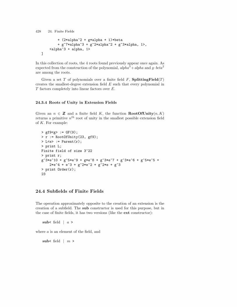
428 24. Finite Fields
+ (2*alpha^2 + g*alpha + 1)*beta+ g^7*alpha^3 + g^2*alpha^2 + g^3*alpha, 1>,
<alpha^3 + alpha, 1>]
In this collection of roots, the 4 roots found previously appear once again. Asexpected from the construction of the polynomial, alpha3+alpha and g ·beta2
are among the roots.
Given a set T of polynomials over a finite field F , SplittingField(T )creates the smallest-degree extension field E such that every polynomial inT factors completely into linear factors over E.
24.3.4 Roots of Unity in Extension Fields
Given an n ∈ ZZ and a finite field K, the function RootOfUnity(n,K)returns a primitive nth root of unity in the smallest possible extension fieldof K. For example:
> gf9<g> := GF(9);> r := RootOfUnity(23, gf9);> L<e> := Parent(r);> print L;Finite field of size 3^22> print r;g^3*e^10 + g^5*e^9 + g*e^8 + g^3*e^7 + g^3*e^6 + g^5*e^5 +
2*e^4 + e^3 + g^2*e^2 + g^2*e + g^3> print Order(r);23
24.4 Subfields of Finite Fields
The operation approximately opposite to the creation of an extension is thecreation of a subfield. The sub constructor is used for this purpose, but inthe case of finite fields, it has two versions (like the ext constructor):
sub< field | a >
where a is an element of the field, and
sub< field | m >

24.5 Embedding a Finite Field in Another Finite Field 429
where m is a positive integer dividing the absolute degree of the original field.The first of these returns the subfield generated by a, and the second returnsa subfield of absolute degree m. Both forms of sub optionally return theembedding monomorphism from the subfield to the main field as a secondvalue. This map has the same effect as a standard coercion.
For instance, the following lines create two fields of size 34, as subfieldsof gf9e4e3 :
> gf9e4e3s4A<gammaA> := sub< gf9e4e3 | alpha^2 >;> gf9e4e3s4B<gammaB> := sub< gf9e4e3 | 4 >;> print gf9e4e3s4A;Finite field of size 3^4> print gf9e4e3s4B;Finite field of size 3^4
Although these fields are isomorphic, because they have the same size, theyhappen to have different defining polynomials, and their generators are notequal. The coercion mapping gives the isomorphism between the fields:
> print DefiningPolynomial(gf9e4e3s4A);$.1^4 + 2*$.1 + 2> print DefiningPolynomial(gf9e4e3s4B);$.1^4 + 2*$.1^3 + 2> print gammaA eq gammaB;false> print gf9e4e3s4A ! gammaB;gammaA^31> print gf9e4e3s4B ! gammaA;gammaB^31
With respect to the field gf9e4 , the generator of gf9e4e3s4A is alpha2, aswould be expected, but the generator of gf9e4e3s4B is g7alpha2:
> print gf9e4 ! gammaA;alpha^2> print gf9e4 ! gammaB;g^7*alpha^2
24.5 Embedding a Finite Field in Another Finite Field
When an extension or subfield is created, Magma automatically creates anembedding monomorphism from the smaller field into the bigger field. This

430 24. Finite Fields
monomorphism permits the user to perform coercions of elements, test rela-tionships between fields, and so on. For instance:
> print gf9e4e3s4A subset gf9e4e3;true> print alpha in gf9e4e3s4B;false
However, if two fields F and F ′ are created independently of one another, thenMagma will not see them as related. Even if they have the same characteristicp, and the degree of F divides the degree of F ′. Magma will not be awareof the mathematical relationship between them. Error messages will arise ifthe user attempts any operations involving both F and F ′. For example:
> gf9e4e11<delta> := ext< gf9e4 | 11 >;> print gf9e4e11;Finite field of size 3^88> print gf9e4e3s4A;Finite field of size 3^4> print gf9e4e3s4A subset gf9e4e11;
>> print gf9e4e3s4A subset gf9e4e11;^
Runtime error in ’subset’: Arguments have no covering field> print gf9e4e11 ! gammaA;
>> print gf9e4e11 ! gammaA;^
Runtime error in ’!’: Illegal coerce
To solve this problem, F must be embedded in F ′, using the procedureEmbed(F, F ′). This procedure sets up an isomorphism between F and thesubfield of F ′ with the same cardinality:
> Embed(gf9e4e3s4A, gf9e4e11);
Now Magma is aware that gf9e4e3s4A is a subfield of gf9e4e7 . After anembedding has taken place, computations and tests involving the two fieldsmay be performed:
> print gf9e4e3s4A subset gf9e4e11;true> print gf9e4e11 ! gammaA;g^3*alpha^2 + 1> print Degree(gf9e4e11), Degree(gf9e4e11, gf9e4e3s4A);

24.5 Embedding a Finite Field in Another Finite Field 431
88 22
The embedding isomorphism is always chosen so that diagrams ‘commute’,that is, so that all the homomorphisms involving the fields are compatible.
In Magma, the ext constructor generates a different field each time it iscalled, even if the arguments given to the constructor are exactly the same.This facility allows the user to create two fields which are isomorphic butnotionally distinct. If a relationship between the two fields is to be establishedthe Embed procedure must be invoked:
> F1 := ext< gf9 | 5 >;> F2 := ext< gf9 | 5 >;> print F1 eq F2;
>> print F1 eq F2;^
Runtime error in ’eq’: Arguments have no covering field> Embed(F1, F2);> print F1 eq F2;true> print DefiningPolynomial(F1) eq DefiningPolynomial(F2);true> print F1.1 eq F2.1;false> print F2 ! (F1.1);F2.1^81> print F1 ! (F2.1);F1.1^729
Although these two fields were created with the same expression, and theirdefining polynomials are the same, their generators do not correspond in theisomorphism. For each field, the algorithm involved has randomly selectedone of the five roots of the defining polynomial to be the generator of thefield.
The GF function is an exception. Every call to GF creates the defaultfield of the given size, so all fields created as GF(p, n) or GF(q), for the samep, n pair or the same q = pn, are identical:
> F3 := GF(7, 3);> F4 := GF(7, 3);> print F3 eq F4;true> print F3.1 eq F4.1;true

432 24. Finite Fields
There is a variant of the Embed function in which the user can specifythe image of the generator. Embed(F, F ′, x) embeds F in F ′ in such a waythat the embedding isomorphism maps the generator of F to the element xof F ′.
24.6 Associated Polynomials
Table 24.1. Polynomials associated with finite fields
Magma Meaning
DefiningPolynomial(F ) Polynomial over the ground field ofF , defining F as an extension of theground field
DefiningPolynomial(F, S) Polynomial over subfield S of F , defin-ing F as an extension of S
IrreduciblePolynomial(F, m) Irreducible polynomial of degree mover F
AllIrreduciblePolynomials(F, m) Set of the monic irreducible polyno-mials of degree m over F
IsIrreducible(f) true if univariate polynomial f overF is irreducible
PrimitivePolynomial(F, m) A primitive polynomial of degree mover F (i.e., irreducible, and having aprimitive root of the degree-m exten-sion field of F as a root)
IsPrimitive(f) true if univariate polynomial f overF is primitive
MinimalPolynomial(a) Minimal polynomial of a ∈ F overground field of F
MinimalPolynomial(a, S) Minimal polynomial of a ∈ F oversubfield S of F
CharacteristicPolynomial(a) Characteristic polynomial of a ∈ Fover ground field of F
CharacteristicPolynomial(a, S) Characteristic polynomial of a ∈ Fover subfield S of F
Several polynomials are associated with finite fields, including definingpolynomials, irreducible polynomials and Conway polynomials as explainedabove. Table 24.1 (p. 432) gives a list of the polynomial functions for finitefields.
A few of these functions resemble the Degree function in that they cantake one argument or two arguments. If only one argument is given, the

24.6 Associated Polynomials 433
operation is performed with respect to the ground field, whereas if two ar-guments are given, the operation is performed with respect to the specifiedsubfield. (However, if no subfield is stated in the Degree function, it is under-stood to be the prime field, not the ground field.) For instance, the functionMinimalPolynomial returns the minimal polynomial of a given element aof the finite field F . If a subfield S of F is given as the second argument,the value returned is the minimal polynomial over the coefficient field S.Otherwise, it is the minimal polynomial over the ground field of F :
> e := beta^3 + 2*g*beta + alpha;> print MinimalPolynomial(e); // i.e., over gf9e4y^3 + (2*alpha^3 + alpha^2 + g^2*alpha + g^2)*y^2 +
(alpha^3 + g^6*alpha^2 + alpha)*y + g^6*alpha^3 + alpha> print MinimalPolynomial(e, gf9);x^12 + 2*x^10 + g^7*x^8 + g^6*x^7 + g^6*x^6 + 2*x^5 + x^4 +
g^7*x^3 + 2*x^2 + g^5*x + g^3> print MinimalPolynomial(e, GF(3));$.1^24 + $.1^22 + $.1^18 + $.1^17 + $.1^16 + 2*$.1^15 +
$.1^14 + 2*$.1^11 + 2*$.1^10 + 2*$.1^9 + 2*$.1^7 +2*$.1^5 + 2*$.1^4 + $.1^2 + 2
> print MinimalPolynomial(e, gf9e4e3);$.1 + (g^6*alpha^3 + g^7*alpha^2 + g)*beta^2 +
(g*alpha^3 + 2*alpha^2 + g^7)*beta + g*alpha^3 +g^5*alpha^2 + g^2*alpha + g^7
Note that the degree of this polynomial indicates the degree of the corre-sponding extension. In the last example, the given element e is in the givensubfield, so the polynomial is linear.
The minimal polynomial of the generator of a field F is the definingpolynomial of F . For example:
> print MinimalPolynomial(beta) eq defgf9e4e3;true
Some remarks should now be made on Conway polynomials. As was shownabove, any irreducible polynomial of degree d over a finite field F may be usedin Magma to create an extension of F of degree d. Since this freedom canbe problematic, there has been defined, for each moderately small prime pand exponent n, a special irreducible polynomial of degree n with coefficientsin GF(p). It is known as the Conway polynomial Cp,n. (The details of thedefinition are given in the Handbook.) Magma contains a list of the knownConway polynomials. In order to avoid the ambiguities that might arise whenembeddings take place, Magma uses a Conway polynomial (if it is known)whenever a field is being defined as an extension of a prime field. For example:

434 24. Finite Fields
Table 24.2. Conway polynomial functions
Magma Meaning
ConwayPolynomial(p, n) Degree-n Conway polynomial over GF(p)
ExistsConwayPolynomial(p, n) If a Conway polynomial of degree n overGF(p) is known, returns true and thepolynomial, else returns false
IsConway(F ) true if defining polynomial of F relativeto its prime field is a Conway polynomial
> print ConwayPolynomial(5, 6) eq DefiningPolynomial(gf5e6);true
Table 24.2 contains the Conway polynomial functions.
24.7 Operations on Finite Field Elements
Magma has functions for several standard operations on elements of finitefields. Some of them are listed in Table 24.3. Notice that for those functionsthat take an optional subfield as a second argument, whenever the subfieldis omitted the default subfield is the prime field, not the ground field as inthe polynomial functions explained above.
One of the most important functions for finite field elements is Log(a).It uses the primitive element w ∈ F that Magma returns from the functionPrimitiveElement(F ). By definition of w, every non-zero a ∈ F may beexpressed as wn for a unique n ∈ 0, . . . , #F − 2. Log(a) returns this valuen. For instance:
> pr := PrimitiveElement(gf9e4);> print pr;alpha^3 + g^5*alpha^2 + g^2*alpha + g^7> print Log(alpha);4879> print pr^4879;alpha> print Log(gf9e4!g);2460> print pr^2460;g
The Log function only applies to moderately small fields, for which Magmacan calculate the complete table of logarithms. These logarithms are called

24.7 Operations on Finite Field Elements 435
Table 24.3. Functions on elements of finite fields
Magma Meaning
Norm(a) Absolute norm of a (norm relative to prime field)
Norm(a, S) Norm of a relative to subfield S
Trace(a) Absolute trace of a (trace relative to prime field)
Trace(a, S) Trace of a relative to subfield S
Log(a) Discrete logarithm of a (6= 0), with ‘base’ the definingprimitive element w, i.e., n such that wn = a
Order(a) Multiplicative order of a (6= 0)
FactoredOrder(a) Multiplicative order of a ( 6= 0) in factored form (as afactorization sequence)
Sqrt(a) A square root of a, if an answer exists
IsSquare(a) If a is square, returns true and a square root, else re-turns false
Root(a, n) An nth root of a, if an answer exists
Eltseq(a) Length-d sequence containing the coefficients of a ∈ Fas a polynomial over S in the generator of F over S,where S is the ground field of F and d is the degree ofF over S
Eltseq(a, S) Length-d sequence containing the coefficients of a ∈ Fas a polynomial over S in the generator of F over S,where S is a subfield of F and d is the degree of F overS
Eltseq(a) Sequence as for Eltseq(a, S), where S is the ground fieldof F
Seqelt(Q, F ) Given a sequence Q as described for Eltseq, returns thecorresponding element of F
Zech logarithms, and they allow arithmetic in the field to be done very effi-ciently by Magma.
ElementToSequence(a, S) and SequenceToElement(Q,S), which arecommonly abbreviated to Eltseq(a, S) and Seqelt(Q,F ), convert betweenan element a of a finite field F and its representation as a polynomial in thegenerator of F over a subfield S, with coefficients in S. Eltseq returns thecoefficients of the polynomial in a length-d sequence Q, where d is the degreeof F over S, and Seqelt returns the field element a. If Eltseq is used in theform Eltseq(a), then the subfield S is understood to be the ground field ofF . For instance:
> print Eltseq(pr);[ g^7, g^2, g^5, 1 ]> print Eltseq(pr, GF(3));[ 0, 0, 2, 0, 0, 2, 2, 1 ]> print Seqelt([ 2*alpha, 1, g*alpha], gf9e4e3);

436 24. Finite Fields
g*alpha*beta^2 + beta + 2*alpha
24.8 Printing Finite Field Elements
There are two ways of printing an element of a finite field in Magma. It caneither be printed as a power of the generating element, or else as a polynomialin the generator over the ground field, having degree less than the relativedegree of the field. For instance, in gf9 , 2g + 2 and g6 are different ways ofexpressing the same element:
> print (2*g + 2) eq g^6;true
Note that the issue does not arise for prime fields, because their elements areprintable as ‘integers’.
Magma is always able to express elements in the polynomial form.(This form resembles the vector representation explained in the next sec-tion and the Eltseq representation discussed above.) However, it can onlyexpress them as powers of the generator if the field is small enough forthe Zech logarithms to be stored. To specify the default style of printingpreferred by the user for all subsequently-created (small) finite fields, theprocedure AssertAttribute(FldFin, "PowerPrinting", b) should be used.The argument b takes a Boolean value: it should be true if elements areto be printed as powers of the generator, and false if they are to beprinted as polynomials. However, this procedure does not change the print-ing style for any fields that have been already created. To change theprinting style for a particular small and non-prime field F , the procedureAssertAttribute(F, "PowerPrinting", b) may be used, with b a Boolean asbefore.
To find the current value of the attribute "PowerPrinting" for a field For for the FldFin category, the user should call the HasAttribute function,as demonstrated below:
> fld := GF(81);> print HasAttribute(fld, "PowerPrinting");true true
> print HasAttribute(FldFin, "PowerPrinting");true true
This function, like the procedure AssertAttribute, is used for several at-tributes throughout the Magma system. Its first return value is a Boolean
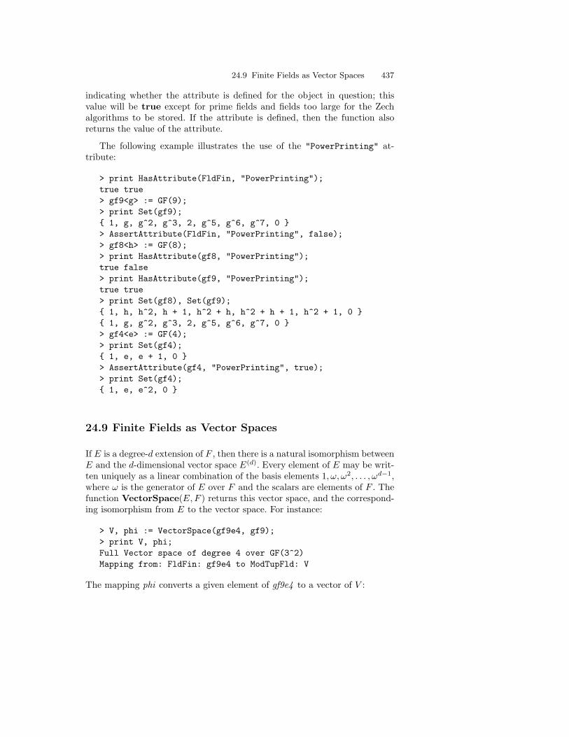
24.9 Finite Fields as Vector Spaces 437
indicating whether the attribute is defined for the object in question; thisvalue will be true except for prime fields and fields too large for the Zechalgorithms to be stored. If the attribute is defined, then the function alsoreturns the value of the attribute.
The following example illustrates the use of the "PowerPrinting" at-tribute:
> print HasAttribute(FldFin, "PowerPrinting");true true> gf9<g> := GF(9);> print Set(gf9); 1, g, g^2, g^3, 2, g^5, g^6, g^7, 0 > AssertAttribute(FldFin, "PowerPrinting", false);> gf8<h> := GF(8);> print HasAttribute(gf8, "PowerPrinting");true false> print HasAttribute(gf9, "PowerPrinting");true true> print Set(gf8), Set(gf9); 1, h, h^2, h + 1, h^2 + h, h^2 + h + 1, h^2 + 1, 0 1, g, g^2, g^3, 2, g^5, g^6, g^7, 0 > gf4<e> := GF(4);> print Set(gf4); 1, e, e + 1, 0 > AssertAttribute(gf4, "PowerPrinting", true);> print Set(gf4); 1, e, e^2, 0
24.9 Finite Fields as Vector Spaces
If E is a degree-d extension of F , then there is a natural isomorphism betweenE and the d-dimensional vector space E(d). Every element of E may be writ-ten uniquely as a linear combination of the basis elements 1, ω, ω2, . . . , ωd−1,where ω is the generator of E over F and the scalars are elements of F . Thefunction VectorSpace(E, F ) returns this vector space, and the correspond-ing isomorphism from E to the vector space. For instance:
> V, phi := VectorSpace(gf9e4, gf9);> print V, phi;Full Vector space of degree 4 over GF(3^2)Mapping from: FldFin: gf9e4 to ModTupFld: V
The mapping phi converts a given element of gf9e4 to a vector of V :

438 24. Finite Fields
> print (g^5*alpha^3 + g^5*alpha^2 + g^3*alpha + 2 ) @ phi;( 2 g^3 g^5 g^5)
The correspondence between the element and its vector space representationis obvious.
Instead of using the powers of the generator as a basis, the user maychoose a basis for the vector space. If B is a suitable sequence of elementsof F , then VectorSpace(E, F, B) returns the vector space and isomorphismfor that basis.
For example, a normal basis for E over F is a basis of the forma, aq, . . . , aqd−1
. Such a basis has the property that exponentiation of an el-ement by a power of 2 can be achieved by rotating the vector representingthat element. If a ∈ E forms a normal basis, it is called a normal element.
The next example shows how to construct a normal basis for a very largefield, the field with 21000 elements. Firstly, the field must be constructed:
> K<w> := FiniteField(2, 1000);
The function IsNormal(a) tests whether a forms a normal basis over theprime field, and NormalElement(E) returns a normal element for thefield E considered over its prime field. (For calculations relative to an arbi-trary subfield S, the functions IsNormal(a, S) and NormalElement(E, S)should be used instead.) In this example, it will be convenient if the generatorof K is normal, so this should be tested:
> print IsNormal(w);false
Unfortunately, w is not normal. Therefore it is necessary to find an elemente which is normal, and then form the basis B:
> e := NormalElement(K);> B := [IsZero(i) select e else Self(i)^2 : i in [0..999]];
Now that B is known, the vector space may be constructed:
> VS, iso := VectorSpace(K, GF(2), B); print VS, iso;Full Vector space of degree 1000 over GF(2)Mapping from: FldFin: K to ModTupFld: VS
Since VS is a vector space with a normal basis, there should be a strongrelationship between the vectors corresponding to r and r(2t), for any fieldelement r and integer t. In fact, the first vector rotated t places will equalthe second vector, as the following output verifies:

24.10 Finite Fields as Matrix Algebras 439
> r := Random(K); t := Random(1, 10);> r2t := r^(2^t);> rVS := r @ iso;> r2tVS := r2t @ iso;> print r2tVS eq VS!Rotate(Eltseq(rVS), t);true
24.10 Finite Fields as Matrix Algebras
Suppose E is a degree-d extension of a finite field F . (F does not have to bethe ground field of E; it may be isomorphic to any subfield of E.) As wasshown above, E is isomorphic to the d-dimensional vector space E(d). How-ever, a stronger mathematical statement can be made. E is also isomorphicto a matrix algebra of degree d and dimension d over F . The advantage ofthis representation is that field elements as matrice can be multiplied andinverses can be found, whereas field elements as vectors can only be addedand made negative. Of course, elements of E which are in the ground fieldF correspond to multiples of the identity matrix, so they still have a scalaraction. The function MatrixAlgebra(E,F ) returns this matrix algebra A,and the corresponding isomorphism from E to A, such that the generator ofE maps to the generator of A. For instance:
> M<G>, isoM := MatrixAlgebra(gf9e4, gf9);> print M, isoM;Matrix Algebra of degree 4 and dimension 4 with 1 generator
over GF(3^2)Mapping from: FldFin: gf9e4 to AlgMat: M> print G eq isoM(alpha);true> print isoM(alpha^2+1) eq G^2+1;true
Observe that G, the generator of M , is isomorphic to alpha, the generator ofgf9e4 . The isomorphism is isoM .
The generator of the matrix algebra is constructed as the companionmatrix of the field’s defining polynomial. It has a line of 1s above the maindiagonal, and 0s elsewhere, except for the last row.
> print G;[ 0 1 0 0][ 0 0 1 0][ 0 0 0 1]

440 24. Finite Fields
[ g 0 g^2 0]> defgf9e4 := DefiningPolynomial(gf9e4); print defgf9e4;x^4 + g^6*x^2 + g^5> print G eq CompanionMatrix(defgf9e4);true
The last row of the generating matrix contains the coefficients of the negativeof the defining polynomial modulo xd. In the present example, the last rowrepresents the polynomial g + 0x + g2x2 + 0x3:
> print -defgf9e4 mod x^4;g^2*x^2 + g> print Coefficients(-defgf9e4 mod x^4);[ g, 0, g^2 ]
In general, the top row of the matrix indicates the vectorial representationof the element as a sum of powers of the generator up to d− 1. For instance:
> m := 2 + G^2 + G^3; print m;[ 2 0 1 1][ g 2 g^2 1][ g g g g^2][g^3 g g^7 g]
Functions such as MinimalPolynomial, CharacteristicPolynomialand Order can be applied to elements of the matrix algebra just as for fieldelements:
> print Order(m);656> print Order(2 + alpha^2 + alpha^3);656
There is a further way of constructing a matrix algebra that involves finitefields. If A is a matrix algebra A over a finite field E, and S is a subfield ofE, then there exists another matrix algebra N over S which is isomorphic toA. N is constructed by expanding each entry of a matrix of A into the blockmatrix associated with it.d The function MatrixAlgebra(A,S) returns thismatrix algebra, and the corresponding isomorphism from E to the matrixalgebra, such that the generator of E maps to the generator of the matrixalgebra. For instance:
> gf3 := GF(3);> N<GN>, isoN := MatrixAlgebra(M, gf3);> print N;

24.10 Finite Fields as Matrix Algebras 441
Matrix Algebra of degree 8 with 1 generator over GF(3)> print GN;[0 0 1 0 0 0 0 0][0 0 0 1 0 0 0 0][0 0 0 0 1 0 0 0][0 0 0 0 0 1 0 0][0 0 0 0 0 0 1 0][0 0 0 0 0 0 0 1][0 1 0 0 1 1 0 0][1 1 0 0 1 2 0 0]> print GN eq isoN(G);true
Each 2×2 block in GN corresponds to an entry of G. Most obviously, a 2×2zero matrix corresponds to a 0 and a 2 × 2 identity matrix corresponds toa 1. In fact, the correspondence comes from yet another matrix algebra, theone relating gf9 to gf3 :
> M9rel3, isoM9rel3 := MatrixAlgebra(gf9, gf3);> print isoM9rel3(g); // block corresponding to g[0 1][1 1]> print isoM9rel3(g^2); // block corresponding to g^2[1 1][1 2]


25. Number Fields
Magma contains very sophisticated machinery for computing in algebraicnumber fields. To the casual user, the specialist features may not be of im-mediate interest. Therefore the earlier sections of this chapter deal mainlywith the easier issues of basic constructions and arithmetic, whereas subse-quent sections treat more complicated structural computations relating tonumber fields and their orders (maximal order, ideal class group, unit group,and Galois group).
A number field is by definition a finite algebraic extension of the rationalfield Q. This means that it is a field containing the rational numbers, inwhich every element satisfies an equation of the form p(x) = 0, where p isa polynomial with rational coefficients. In fact, any number field N consistsof all elements of the form a0 + a1α + · · ·+ an−1α
n−1, for rational numbersai, some non-negative integer n, and a fixed α (called a primitive element forN). The element α can always be chosen such that f(α) = 0 for some monicirreducible polynomial f with integer coefficients; in that case n above willequal the degree of f and is called the degree of the number field. The fieldN is then usually denoted Q(α), and is entirely determined by the definingpolynomial f . As a ring, N is isomorphic to Q[x]/f(x), the quotient of thepolynomial ring over Q and the ideal generated by f .
For example, if f equals x3−2, an irreducible monic polynomial of degree3, a cubic number field may be obtained by adjoining a root α of f to Q. Sucha root is usually referred to as 3
√2, and the resulting field Q( 3
√2) consists of
all rational combinations a0+a13√
2+a23√
22. Higher powers of 3
√2 can simply
be reduced, using the fact that the third power equals 2.
For the sake of efficiency, number fields in Magma are implemented in fourdifferent categories: the field of rational numbers; quadratic number fields;cyclotomic number fields; and ‘general’ number fields. Since rational numbersand ordinary integers have been discussed in detail in Chapter 20, they willonly be mentioned in this chapter occasionally. Most functions for numberfields apply to the rational field as well, with trivial results.
The simplest number field is Q itself; the Magma category for it isFldRat. Next in terms of complexity are quadratic fields, defined by an

444 25. Number Fields
irreducible polynomial f of degree 2. These are the familiar fields obtainedby adjoining the square root of an integer to the rational field, such as Q(
√5).
Quadratic fields have their own category, FldQuad, to take advantage of theexistence of faster algorithms than those available for general number fields,which form the category FldNum. There is one more category of specialnumber fields, namely that of cyclotomic fields, FldCyc. These are obtainedby adjoining a root of unity to Q, that is, an element ζ satisfying ζn = 1 forsome n > 2. Cyclotomic fields can have arbitrary degree, but because theirelements are combinations of roots of unity they arise frequently, for exam-ple in representation theory. Quadratic fields, cyclotomic fields and generalnumber fields will be described in detail below.
Besides these fields, this chapter also discusses orders, which arise as sub-rings of the ring of integers of a field. They have their own Magma categories,RngQuad and RngOrd, corresponding to the quadratic and the generalnumber fields, respectively.
25.1 Elementary Constructions of Number Fields
This section explains how to create number fields and their elements in thevarious categories. The constructions are kept at their simplest level; moresophisticated constructions are discussed later in the chapter.
25.1.1 Number Fields
Table 25.1. Number field functions
Magma Meaning
NumberField(f) Number field Q(α), where α is a root of themonic irreducible integer polynomial f
Degree(K) Absolute degree m = [K : Q] of number fieldK
DefiningPolynomial(K) Monic irreducible degree-m polynomial defin-ing K
Discriminant(K) Discrimant of K
ReducedDiscriminant(K) Reduced discrimant of K
Signature(K) Signature r, s of K
PrimitiveElement(K) A primitive element for K over ground field
Eltseq(a) Sequence [a0, a1 . . . , am−1], where a = a0 +a1α + · · ·+ am−1α
m−1m

25.1 Elementary Constructions of Number Fields 445
The number field K = Q(α) is defined to be the field obtained by adjoin-ing to the rational field Q a root α of the monic irreducible integer polynomialf . K may be created in Magma using the function NumberField(f), wheref is a monic polynomial over ZZ or Q which is irreducible over Q. If the coeffi-cients of f are all integral, a root of f is adjoined to Q to create the extensionK; otherwise, if denominators greater than 1 occur among the coefficients off , an equivalent integral polynomial is used. For example, the following linescreate the field K = Q(
√2 +
√5), by adjoining to Q a root alpha of the
polynomial f = x4 − 14x2 + 9 over Q:
> P<x> := PolynomialRing(IntegerRing());> f := x^4 - 14*x^2 + 9;> K<alpha> := NumberField(f);> print K;NumberField( alpha^4 - 14*alpha^2 + 9 )> print Degree(K);4
Here alpha is an identifier whose value is the root that has been adjoined,and also the printname for this root.
The easiest way to construct elements of K is in terms of alpha. Arithmeticon these elements involves the usual operations.
> t := alpha^2 + 5;> print 5*alpha*t^3 - 2*t + 4*alpha;2360*alpha^3 - 2*alpha^2 - 676*alpha - 10
Another way to create elements of K is to coerce into K a sequence of integersor rationals whose length is the degree of K:
> print K![5, 0, 1, 0];alpha^2 + 5
When elements are created in this way, Magma interprets the contents ofthe sequence as coefficients of a polynomial in α, starting with the constantterm. If the sequence is [a0, a1 . . . , am−1] then the corresponding element isa0 + a1α + · · ·+ am−1α
m−1. The function Eltseq(a) reverses this process:
> print Eltseq(2*t + 3);[ 13, 0, 2, 0 ]
Table 25.1 lists some access functions for a number field K. The meaningof all of these should be clear, except perhaps in the case of Signature.The signature of K consists of two natural numbers, usually called r and s,

446 25. Number Fields
being the number of real roots and of pairs of complex roots of the definingpolynomial of the field. Real roots correspond to ways of embedding the fieldin the real numbers, and complex non-real roots to (pairs of) embeddings inthe complex numbers. Since the total number of roots equals the degree mof the polynomial (and the field), it follows that m = r + 2 · s.
25.1.2 Quadratic Fields
Table 25.2. Quadratic field functions
Magma Meaning
QuadraticField(m) Quadratic field Q(√
d), where d is the square-freepart of the non-square integer m
Degree(K) Degree of quadratic field K over Q (always equals2)
DefiningPolynomial(K) Monic irreducible quadratic polynomial defining K
Discriminant(K) Discrimant of K = Q(√
d) (equals d if d ≡ 0 or 1(mod 4), else 4d
Signature(K) Signature r, s of K (2, 0 if d > 0, else 0, 1)
Eltseq(a) Sequence [a0, a1], where a = a0 + a1
√d
The quadratic field Q(√
d), where d is a (positive or negative) square-freeinteger, may be created in Magma with the function QuadraticField. Thisis an alternative and preferable way of constructing the number field obtainedby adjoining a root of x2 − d to Q. For example:
> QF7<rt7> := QuadraticField(7);> print QF7;Quadratic Field Q(rt7)> print rt7^2;7
If the argument m of QuadraticField(m) contains any square factors,Magma will divide out the largest possible square from m to obtain thesquare-free integer d, and then create Q(
√d). For instance, if m = 20, then
the generator of the resulting quadratic field will be equal to√
5:
> Q<w> := QuadraticField(20);> print Q, w^2, (1+w)^2;Quadratic Field Q(w)5 6 + 2*w

25.1 Elementary Constructions of Number Fields 447
It is usual to create quadratic fields (and other number fields) with a generatorassignment statement. If no generator name is given, then the generator isprinted using sqrt-d:
> Gaussians := QuadraticField(-1);> print Gaussians.1;sqrt-1
The elements of a quadratic field are of the form a0 + a1√
m, where a0
and a1 are rational numbers. These elements may be created in Magmaeither as expressions in
√d (as above), or by coercing into the field a se-
quence of rationals [a0, a1]. Conversely, the (rational) coefficients [a0, a1]of an element a may be extracted with the function Eltseq(a), whichis short for ElementToSequence(a). Elements are printed in the form(1/m) · (u + v
√d), where u, v, m are integers, the denominator m is positive
and gcd(u, v,m) = 1. For example, the following lines construct and printthe elements f = 1
3 − 56
√7 and g = 5
8 + 6√
7, their sum, and the sequencerepresentation of their product:
> f := QF7![1/3, -5/6]; print f;1/6*(2 - 5*rt7)> g := QF7![5/8, 6]; print g;1/8*(5 + 48*rt7)> print f + g;1/24*(23 + 124*rt7)> print Eltseq(f * g);[ -835/24, 71/48 ]
The main access functions for quadratic fields are listed in Table 25.2.
25.1.3 Cyclotomic Fields
The field K = Q(ζm), where m is an integer greater than 2, is called thecyclotomic number field of cyclotomic order m. It is the field created by ad-joining to Q a primitive mth root of unity, and it is constructed with thefunction CyclotomicField(m). The degree d of K (and of its defining poly-nomial) is equal to φ(m); it may be obtained as Degree(K) or EulerPhi(m).The primitive root of K may be considered as the complex number e
2πim . For
example:
> C8<z> := CyclotomicField(8);> print C8;Cyclotomic Field of order 8 and degree 4

448 25. Number Fields
Table 25.3. Cyclotomic field functions
Magma Meaning
CyclotomicField(m) Cyclotomic field Q(ζm)
CyclotomicOrder(K) m for K = Q(ζm)
Degree(K) Degree d = φ(m) of K = Q(ζm)
DefiningPolynomial(K) Monic irreducible degree-d polynomial defining K
Discriminant(K) Discrimant of K
Signature(K) Signature 0, d2
of K
Conductor(K) Smallest n such that K ⊂ Q(ζn), i.e., m2
if m ≡2 mod 4, else m
Eltseq(a) Sequence [a0, a1 . . . , ad−1], where a = a0 + a1ζm +
· · ·+ ad−1ζd−1m
RootOfUnity(n, K) nth root of unity, as an element of K (if it exists)
VectorSpace(K, E) Vector space V = E(n) and mapping from K ontoV , where E is a subfield of cyclotomic field K suchthat K has degree n over E (uses powers of gener-ator of K as basis)
VectorSpace(K, E, Q) As above, using sequence Q of field elements as abasis
> print z^8;1> print DefiningPolynomial(C8);$.1^4 + 1
Elements of K = Q(ζm) can be created as the values of expressions in-volving the primitive element and rational numbers. Alternatively, the usercan coerce into K a sequence [a0, a1 . . . , at−1] of rational numbers, where t isany non-negative integer, to represent the element a0 +a1ζm + · · ·+at−1ζ
t−1m .
In either case, the elements will be stored and printed in the form a0+a1ζm+· · ·+ad−1ζ
d−1m , where d is the degree of K and the ai are rational; this repre-
sentation is unique, since ζ0m, . . . , ζd−1
m forms a Q-basis for K. Given a ∈ K,the function Eltseq(a) returns the sequence [a0, a1 . . . , ad−1] representing ain this way. For example:
> print 3*z^10 - 5 + 2/5*z^3;2/5*z^3 + 3*z^2 - 5> print C8 ! [2/7, 3/10];3/10*z + 2/7> ee := C8![9, 56, 0, 1, 7/10, 0, 2/3, 0]; print ee;z^3 - 2/3*z^2 + 56*z + 83/10> print Eltseq(ee);[ 83/10, 56, -2/3, 1 ]

25.2 Equation Orders and Maximal Orders 449
A VectorSpace function is provided for viewing a cyclotomic field asa vector space over some subfield. If K is a cyclotomic field with genera-tor w and E is a subfield of K such that K is of degree n over E, thenVectorSpace(K, E) returns the vector space V = E(n) together with theisomorphism from K onto V such that wi is mapped to the (i + 1)th unitvector of V . Similarly, if Q is a length-n sequence of elements of K describinga basis of K over E, then VectorSpace(K,E, Q) returns V = E(n) togetherwith the isomorphism from K onto V such that Q[i] is mapped to the (i+1)th
unit vector of V .
Table 25.3 shows the simple functions for cyclotomic fields.
25.2 Equation Orders and Maximal Orders
Certain subrings of number fields are of great importance in number theory,namely orders. They form the analogue to the ring ZZ with respect to thefield Q. The most important orders in a number field N = Q(α) are theequation order EN and the maximal order MN . The equation order consistsof all combinations of powers of α with integer coefficients: EN = ZZ[α]. Themaximal order MN is the subring of N consisting of all elements β of N thatsatisfy a polynomial equation g(β) = 0 for some polynomial g with integercoefficients. Since α itself satisfies such a polynomial equation (with g = f ,the defining polynomial of N), it is clear that EN ⊆ MN . In a sense the ringMN consists of all ‘integers’ in N (satisfying an integer relation), and so it isoften called the ring of integers of N . All orders of N are subrings of MN .
In the simplest number field, Q, both the equation order and the maximalorder equal the ring of ordinary integers, ZZ; this is the only order in Q. Incyclotomic fields, it is also the case that the equation order and the maximalorder are equal. Therefore, if K is a cyclotomic or rational field and a ∈ K,then a is in the maximal order of K if and only if its coefficients are integral.Magma does not offer any functions for orders of Q or cyclotomic fields.
However, if K is a quadratic field or a general number field then thetwo orders may be different. Consequently, Magma offers the functionsEquationOrder(K) and MaximalOrder(K) in these categories. (Thenumber field can be retrieved from the equation order with the functionFieldOfFractions.) Orders in quadratic fields and in general number fieldshave their own categories, RngQuad and RngOrd. Table 25.4 lists severalfunctions relating to orders of number fields; some of these functions are onlyprovided for certain categories.
For example, consider the field Q(√
5). The equation order is ZZ[√
5], whichconsists of all elements a+b
√5, where a and b are integers. Now, the element

450 25. Number Fields
Table 25.4. Orders of number fields
Magma Meaning
EquationOrder(K) Equation order of number field K
EquationOrder(f) Equation order defined by monic irreducible in-teger polynomial f
MaximalOrder(K) Maximal order (ring of integers) of K
MaximalOrder(f) Equation order defined by monic irreducible in-teger polynomial f
IntegerRing(K) Maximal order (ring of integers) of K
FieldOfFractions(O) Field of fractions of order O
IsEquationOrder(O) true if O is an equation order (i.e., its basis isa power basis)
IsMaximal(O) true if O equals maximal order over its field offractions
IntegralBasis(K) A basis for K consisting of integral elements
IsIntegral(a) true if element a is in the maximal order of K
Conductor(K) Order of smallest cyclotomic field containing K
DefiningPolynomial(O) Defining polynomial for order O over its groundring
Degree(O) Degree of order O
Discriminant(O) Discriminant of order O
ReducedDiscriminant(O) Reduced discriminant of order O
Signature(O) Signature r, s of order O
(1 +√
5)/2 is not in the equation order, but since it satisfies x2 − x− 1 = 0,it is contained in the maximal order. Therefore the maximal order is strictlygreater than the equation order for this field. The following lines show howto define these orders, firstly in a quadratic field, and secondly in a generalnumber field:
> // quadratic field> Q5<rt5> := QuadraticField(5);> EO := EquationOrder(Q5);> print EO;Order of conductor 2 in Quadratic Field Q(sqrt5)> MO := MaximalOrder(Q5);> print MO;Order of conductor 1 in Quadratic Field Q(sqrt5)> a := (1 + rt5) / 2;> print a in EO;false> print a in MO;true

25.2 Equation Orders and Maximal Orders 451
> print IsIntegral(a);true
> // number field> P<x> := PolynomialRing(RationalField());> Q5<rt5> := NumberField(x^2 - 5);> EO := EquationOrder(Q5);> print EO;Equation Order of Q5> MO := MaximalOrder(Q5);> print MO;Maximal Order of Q5> a := (1 + rt5) / 2;> print a notin EO and a in MO;true
The facilities for orders in the different categories will now be discussedin more detail.
25.2.1 Orders in Quadratic Fields
For a quadratic field K = Q(√
d), the computation of the maximal order MK
is easy. It depends solely on the residue class of d modulo 4, irrespective ofwhether d is positive or negative. If d ≡ 2, 3 (mod 4) then MK equals theequation order EK ; for d ≡ 1 (mod 4), MK = ZZ + ZZ · (1 +
√d)/2, so it
is larger than EK . Let εd =√
d for d ≡ 2, 3 (mod 4) and εd = (1 +√
d)/2for d ≡ 1 (mod 4); then the maximal order will always consist of integerlinear combinations of 1 and εd. That is, [1, εd] forms an integral basis forthe field, returned by the function IntegralBasis(K) (as a sequence of fieldelements) or Basis(MK) (as a sequence of elements of MK). This εd willbe the ‘generator’ for the maximal order. It may be given an identifier andprintname by means of generator assignment; otherwise, it will be printed asepsilond. For instance:
> Q<w> := QuadraticField(-3);> M<z> := MaximalOrder(Q);> print IntegralBasis(Q);[ 1, 1/2*(1 + w) ]> print z, Q ! z;z 1/2*(1 + w)> print M ! w;-1 + 2*z
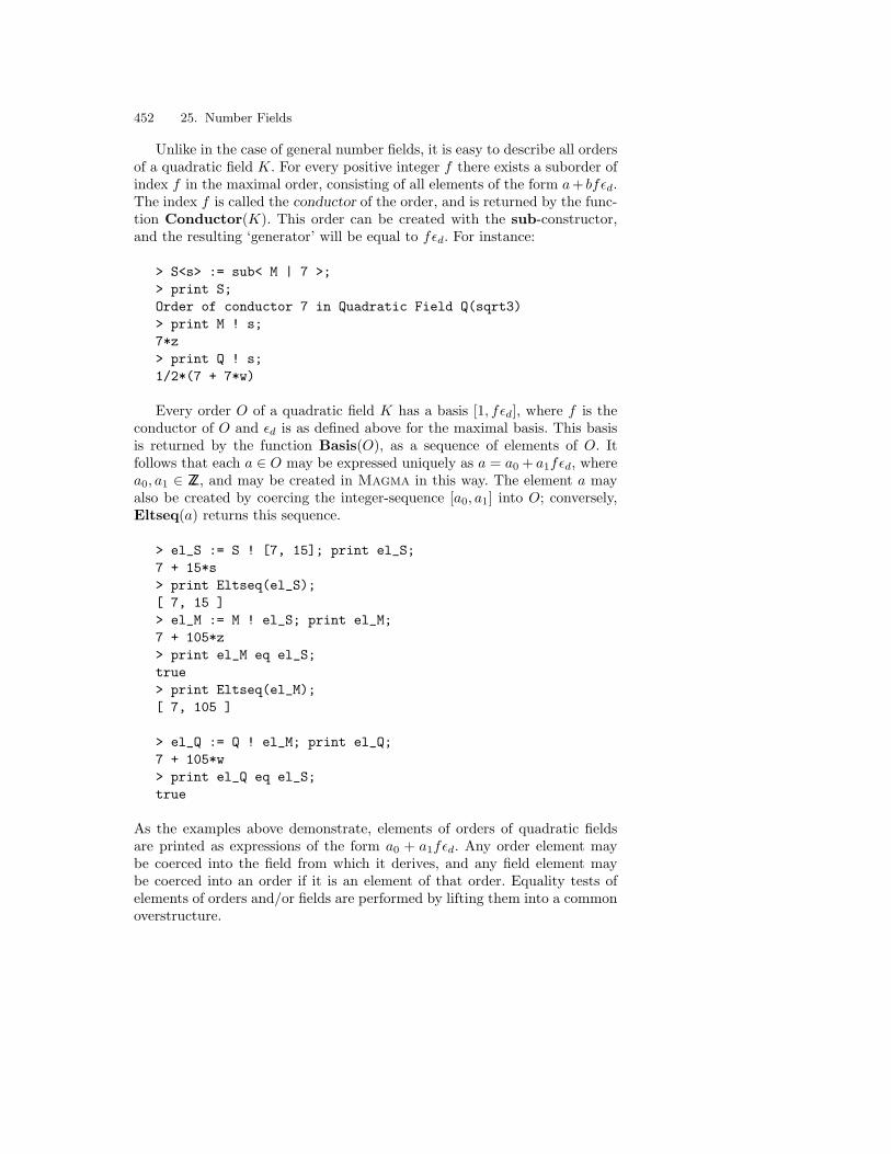
452 25. Number Fields
Unlike in the case of general number fields, it is easy to describe all ordersof a quadratic field K. For every positive integer f there exists a suborder ofindex f in the maximal order, consisting of all elements of the form a+ bfεd.The index f is called the conductor of the order, and is returned by the func-tion Conductor(K). This order can be created with the sub-constructor,and the resulting ‘generator’ will be equal to fεd. For instance:
> S<s> := sub< M | 7 >;> print S;Order of conductor 7 in Quadratic Field Q(sqrt3)> print M ! s;7*z> print Q ! s;1/2*(7 + 7*w)
Every order O of a quadratic field K has a basis [1, fεd], where f is theconductor of O and εd is as defined above for the maximal basis. This basisis returned by the function Basis(O), as a sequence of elements of O. Itfollows that each a ∈ O may be expressed uniquely as a = a0 + a1fεd, wherea0, a1 ∈ ZZ, and may be created in Magma in this way. The element a mayalso be created by coercing the integer-sequence [a0, a1] into O; conversely,Eltseq(a) returns this sequence.
> el_S := S ! [7, 15]; print el_S;7 + 15*s> print Eltseq(el_S);[ 7, 15 ]> el_M := M ! el_S; print el_M;7 + 105*z> print el_M eq el_S;true> print Eltseq(el_M);[ 7, 105 ]
> el_Q := Q ! el_M; print el_Q;7 + 105*w> print el_Q eq el_S;true
As the examples above demonstrate, elements of orders of quadratic fieldsare printed as expressions of the form a0 + a1fεd. Any order element maybe coerced into the field from which it derives, and any field element maybe coerced into an order if it is an element of that order. Equality tests ofelements of orders and/or fields are performed by lifting them into a commonoverstructure.
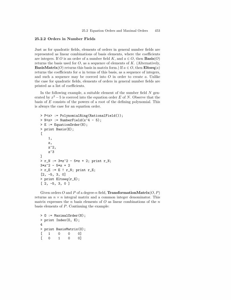
25.2 Equation Orders and Maximal Orders 453
25.2.2 Orders in Number Fields
Just as for quadratic fields, elements of orders in general number fields arerepresented as linear combinations of basis elements, where the coefficientsare integers. If O is an order of a number field K, and a ∈ O, then Basis(O)returns the basis used for O, as a sequence of elements of K. (Alternatively,BasisMatrix(O) returns this basis in matrix form.) If a ∈ O, then Eltseq(a)returns the coefficients for a in terms of this basis, as a sequence of integers,and such a sequence may be coerced into O in order to create a. Unlikethe case for quadratic fields, elements of orders in general number fields areprinted as a list of coefficients.
In the following example, a suitable element of the number field N gen-erated by x2− 5 is coerced into the equation order E of N . Observe that thebasis of E consists of the powers of a root of the defining polynomial. Thisis always the case for an equation order.
> P<x> := PolynomialRing(RationalField());> N<z> := NumberField(x^4 - 5);> E := EquationOrder(N);> print Basis(E);[
1,z,z^2,z^3
]> r_N := 3*z^2 - 5*z + 2; print r_N;3*z^2 - 5*z + 2> r_E := E ! r_N; print r_E;[2, -5, 3, 0]> print Eltseq(r_E);[ 2, -5, 3, 0 ]
Given orders O and P of a degree-n field, TransformationMatrix(O, P )returns an n × n integral matrix and a common integer denominator. Thismatrix expresses the n basis elements of O as linear combinations of the nbasis elements of P . Continuing the example:
> O := MaximalOrder(N);> print Index(O, E);4> print BasisMatrix(O);[ 1 0 0 0][ 0 1 0 0]

454 25. Number Fields
[-1/2 0 1/2 0][-1/2 -1/2 -1/2 1/2]> r_O := O ! r_E; print r_O;[5, -5, 6, 0]
> TM, d := TransformationMatrix(E, O); print TM, d;[1 0 0 0][0 1 0 0][1 0 2 0][2 1 2 2]1> V := RSpace(IntegerRing(), 4);> vec_r_E := V ! Eltseq(r_E);> print vec_r_E * TM;( 5 -5 6 0)> print Eltseq($1) eq Eltseq(r_O);true
Table 25.5. Basis and matrix functions for orders of number fields
Magma Meaning
Basis(O) Basis of field elements for the order O
BasisMatrix(O) Rational matrix representing a basis for O
TraceMatrix(O) Matrix consisting of traces of products ofbasis elements
RepresentationMatrix(a) Representation matrix for order element orfield element a
MultiplicationTable(O) Length-n sequence of representation matri-ces for basis elements of O
TransformationMatrix(O, P ) Transformation matrix from order O to or-der P
IsRelative(O) true if O is given by a transformation ma-trix (i.e., it is not an equation order)
If a is a field element or order element, RepresentationMatrix(a) re-turns the square matrix representing the linear transformation induced bymultiplying by a. For field elements the representation matrix is with respectto the (possibly relative) power basis for the field, whereas for order elementsthe (absolute) basis for the order is used. For example:
> print RepresentationMatrix(z); // field element[0 0 0 5][1 0 0 0]

25.3 Elements of Number Fields and Their Orders 455
[0 1 0 0][0 0 1 0]
> print r_O * O!z;[1, 5, -4, 6]> rm_z_O := RepresentationMatrix(O!z); // order element> print rm_z_O;[ 0 1 1 1][ 1 0 0 -1][ 0 2 1 -2][ 0 0 1 -1]> vec_r_O := V ! Eltseq(r_O);> print vec_r_O * Transpose(rm_z_O);( 1 5 -4 6)
Table 25.5 lists the basis and matrix functions for orders of number fields.
25.3 Elements of Number Fields and Their Orders
Table 25.6. Functions on elements of number fields or orders
Magma Meaning
Norm(a) Product of all the conjugates of a (over groundfield)
Trace(a) Sum of all the conjugates of a (over ground field)
MinimalPolynomial(a) Minimal polynomial of a (over ground field)
NormEquation(O, m) Seeks elements of order O with norm m up to aunit; returns Boolean stating whether any solu-tions exist, and (if true) a sequence of the solutions
NormEquation(O, m) As above, where O is the equation order of field K(category FldQuad or FldNum)
IsIntegral(a) true if element a is integral
IsUnit(a) true if a is a unit
Most functions and arithmetic operators for elements of a number fieldK are also available for elements of orders of K. Table 25.6 lists the mainfunctions for field elements and order elements in the various categories.
As will be explained later, in the FldNum category it is possible to con-struct relative extensions, that is, extensions of a field N other than Q. In thiscase, the return values of Norm, Trace and MinimalPolynomial are given
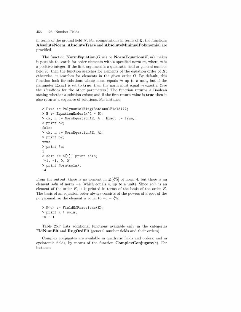
456 25. Number Fields
in terms of the ground field N . For computations in terms of Q, the functionsAbsoluteNorm, AbsoluteTrace and AbsoluteMinimalPolynomial areprovided.
The function NormEquation(O, m) or NormEquation(K,m) makesit possible to search for order elements with a specified norm m, where m isa positive integer. If the first argument is a quadratic field or general numberfield K, then the function searches for elements of the equation order of K;otherwise, it searches for elements in the given order O. By default, thisfunction look for solutions whose norm equals m up to a unit, but if theparameter Exact is set to true, then the norm must equal m exactly. (Seethe Handbook for the other parameters.) The function returns a Booleanstating whether a solution exists; and if the first return value is true then italso returns a sequence of solutions. For instance:
> P<x> := PolynomialRing(RationalField());> E := EquationOrder(x^4 - 5);> ok, n := NormEquation(E, 4 : Exact := true);> print ok;false> ok, n := NormEquation(E, 4);> print ok;true> print #n;1> soln := n[1]; print soln;[-1, -1, 0, 0]> print Norm(soln);-4
From the output, there is no element in ZZ[ 4√
5] of norm 4, but there is anelement soln of norm −4 (which equals 4, up to a unit). Since soln is anelement of the order E, it is printed in terms of the basis of the order E.The basis of an equation order always consists of the powers of a root of thepolynomial, so the element is equal to −1− 4
√5:
> K<w> := FieldOfFractions(E);> print K ! soln;-w - 1
Table 25.7 lists additional functions available only in the categoriesFldNumElt and RngOrdElt (general number fields and their orders).
Complex conjugates are available in quadratic fields and orders, and incyclotomic fields, by means of the function ComplexConjugate(a). Forinstance:
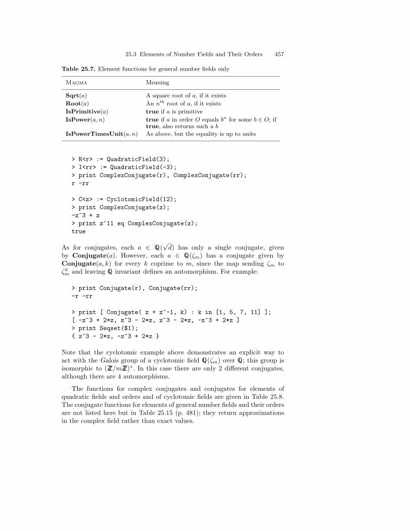
25.3 Elements of Number Fields and Their Orders 457
Table 25.7. Element functions for general number fields only
Magma Meaning
Sqrt(a) A square root of a, if it exists
Root(a) An nth root of a, if it exists
IsPrimitive(a) true if a is primitive
IsPower(a, n) true if a in order O equals bn for some b ∈ O; iftrue, also returns such a b
IsPowerTimesUnit(a, n) As above, but the equality is up to units
> R<r> := QuadraticField(3);> I<rr> := QuadraticField(-3);> print ComplexConjugate(r), ComplexConjugate(rr);r -rr
> C<z> := CyclotomicField(12);> print ComplexConjugate(z);-z^3 + z> print z^11 eq ComplexConjugate(z);true
As for conjugates, each a ∈ Q(√
d) has only a single conjugate, givenby Conjugate(a). However, each a ∈ Q(ζm) has a conjugate given byConjugate(a, k) for every k coprime to m, since the map sending ζm toζkm and leaving Q invariant defines an automorphism. For example:
> print Conjugate(r), Conjugate(rr);-r -rr
> print [ Conjugate( z + z^-1, k) : k in [1, 5, 7, 11] ];[ -z^3 + 2*z, z^3 - 2*z, z^3 - 2*z, -z^3 + 2*z ]> print Seqset($1); z^3 - 2*z, -z^3 + 2*z
Note that the cyclotomic example above demonstrates an explicit way toact with the Galois group of a cyclotomic field Q(ζm) over Q; this group isisomorphic to (ZZ/mZZ)∗. In this case there are only 2 different conjugates,although there are 4 automorphisms.
The functions for complex conjugates and conjugates for elements ofquadratic fields and orders and of cyclotomic fields are given in Table 25.8.The conjugate functions for elements of general number fields and their ordersare not listed here but in Table 25.15 (p. 481); they return approximationsin the complex field rather than exact values.

458 25. Number Fields
Table 25.8. Conjugate functions in quadratic and cyclotomic fields
Magma Meaning
Conjugate(a) Given a = a0 +a1
√d in Q(
√d) or an order, return
a0 − a1
√d
ComplexConjugate(a) Given a = a0 +a1
√d in Q(
√d) or an order, return
a if d > 0, else a0 − a1
√d
Conjugate(a, k) kth conjugate of a ∈ Q(ζm), where gcd(k, m) = 1,
obtained by applying field automorphism ζm 7→ ζkm
ComplexConjugate(a) Complex conjugate of a ∈ Q(ζm)
Quadratic and cyclotomic field elements can be automatically coercedinto a complex field (or IR, Q, or ZZ if they lie in that subfield or subring).Magma’s designers have made a choice of embedding: ζn is sent to e2πi/n,and
√d for d < 0 is sent to
√−di. These embeddings are customary andconvenient (but not necessary). For instance:
> print ComplexField() ! rr;1.73205080756887729352744634149*i> print IntegerRing() ! ( rr * ComplexConjugate(rr));3> print ComplexField() ! z;0.866025403784438646763723170759426544989 +0.499999999999999999999999999987*i
25.4 Advanced Constructions of Fields and Elements
This section discusses advanced methods of creating number fields: the useof roots of unity in cyclotomic fields; the construction of subfields; and theconstruction of relative and multiple extensions.
25.4.1 Cyclotomic Fields and Roots of Unity
In situations where (only) roots of unity are involved in computations, thefunction RootOfUnity is of assistance in constructing such elements in theappropriate cyclotomic field. One version of this function, RootOfUnity(n)takes a positive integer n and returns a primitive nth root of unity ζn inQ(ζn). For example:
> r := RootOfUnity(5); print r;

25.4 Advanced Constructions of Fields and Elements 459
zeta_5> s := RootOfUnity(7); print s;zeta_7> print Parent(r), Parent(s);Cyclotomic Field of order 5 and degree 4Cyclotomic Field of order 7 and degree 6
Automatic coercion enables arithmetic with various roots of unity, mixedwith rationals:
> print (r + s - 2/3)^2;zeta_35^14 + 2*zeta_35^12 + zeta_35^10
- 4/3*zeta_35^7 - 4/3*zeta_35^5 + 4/9
There is a second version of this function, RootOfUnity(n,K), which cre-ates the desired element ζn inside a given cyclotomic field K = Q(ζm). Ofcourse, this is only possible if such an element exists in K, so n must dividem (or 2m if m is odd).
Suppose that the user wishes to work with matrices whose entries areof the form cos(2πi/r) and sin(2πi/r) for certain integers r. It is helpfulto begin by defining short functions that create these sines and cosines asalgebraic numbers. Magma’s designers have made a choice of embedding ζn
in the complex numbers, by sending ζn to e2πi/n, which is customary andconvenient. This makes it possible to express the sines and cosines in termsof roots of unity:
> cos := func< r | (x + x^-1)/2 where x is RootOfUnity(r) >;> sin := func< r | -RootOfUnity(4) * (x - x^-1)/2
where x is RootOfUnity(r) >;> print sin(6);-1/2*zeta_12^3 + zeta_12> print sin(6)^2 + cos(6)^2;1
The following lines use the functions cos and sin to build 3×3 matrices whoseentries are sines and cosines of 2πi/3 and 2πi/5. To create the appropriatematrix ring, it is necessary to find a single cyclotomic field containing allthese algebraic elements. Fortunately it is easy to compute such a field, sincerth and sth roots of unity will be contained in the field of Lth roots of unity,where L = lcm(r, s). In the present example, third roots and fifth roots ofunity are required, as well as fourth roots for the sin function. Therefore thefield Q(ζ60) will suffice, 60 being the least common multiple of 3, 5, and 4:
> MR := MatrixRing(CyclotomicField(60), 3);

460 25. Number Fields
> m1 := MR ! [ cos(3),sin(3),0,sin(3),-cos(3),0,0,0,-1 ];> m2 := MR ! [cos(5),sin(5),0,-sin(5),cos(5),0,0,0,1 ];> print m1 * m2 * m1 eq m2^-1;true
It should be remarked that Magma’s automatic coercion mechanism isalso capable of finding the smallest cyclotomic field containing various roots ofunity. For example, if the user constructs a sequence containing cos(2π/5) andsin(2π/3), Magma will calculate its universe as Q(ζ60), and an element a ex-tracted from the sequence will have this field as its parent. Furthermore, givenany cyclotomic field element a, it is possible to compute the element whichequals a but is a member of the smallest possible cyclotomic field: the func-tion Minimize(a) returns this element; and the procedure Minimize(˜a)mutates a into this element. (Minimize may also be applied to a set ofcyclotomic field elements.) For instance:
> s := [ cos(5), sin(3) ];> print Universe(s);Cyclotomic Field of order 60 and degree 16> a := s[1];> print a;-1/2*zeta_60^14 + 1/2*zeta_60^6 + 1/2*zeta_60^4 - 1/2> print Parent(a);Cyclotomic Field of order 60 and degree 16> Minimize(~a);> print a;-1/2*zeta_5^3 - 1/2*zeta_5^2 - 1/2> print Parent(a);Cyclotomic Field of order 5 and degree 4
The function MinimalField, which may be applied to a cyclotomic fieldelement or a set of such elements, performs a similar task to Minimize. Itreturns the smallest cyclotomic field containing the element(s):
> print MinimalField(s[2]);Cyclotomic Field of order 12 and degree 4
25.4.2 Subfields of Cyclotomic Fields
Sometimes the need arises to mix roots of unity and other algebraic numbers.Sums of roots of unity may define elements in subfields of cyclotomic fields,and it may be convenient to recognize such a situation (e.g., when the subfieldis a quadratic field).

25.4 Advanced Constructions of Fields and Elements 461
In fact, Magma handles automatic coercion from quadratic fields to cy-clotomic fields: if a quadratic field element is contained in a cyclotomic field,it can be coerced into it. This provides a way to write quadratic field elementsas sums of roots of unity. For instance:
> Q<w> := QuadraticField(5);> C<z> := CyclotomicField(5);> print C ! w;-2*z^3 - 2*z^2 - 1
It is not hard to determine the smallest cyclotomic field containing aquadratic field, but the intrinsic function Conductor(K) is also providedfor this:
> Q<w> := QuadraticField(-13);> C<z> := CyclotomicField(Conductor(Q));> print C;Cyclotomic Field of order 52 and degree 24> print C ! w;-2*z^21 + 2*z^19 + 2*z^15 - z^13 + 2*z^11 + 2*z^7 - 2*z^5
It can be more difficult to go the other way, and recognize the subfield in whicha combination of roots of unity lies. The following examples are intended tosuggest helpful techniques.
To find out if a given cyclotomic field element a is contained in somesubfield, the function MinimalPolynomial(a) can be used. The polynomialresulting from this function will define a number field containing the element.For example, the following lines show that ζ7 + ζ6
7 is contained in the cubicfield defined by adjoining a root of x3 + x2 − x− 1, and that ζ7 + ζ2
7 + ζ67 is
contained in a quadratic field which is isomorphic to Q(√−7):
> R<x> := PolynomialRing(RationalField());> C<z> := CyclotomicField(7);> print MinimalPolynomial(z + z^6);x^3 + x^2 - x - 1> mp := MinimalPolynomial(z + z^2 + z^4); print mp;x^2 + x + 2> print Discriminant(mp);-7
The next example is more elaborate. By using a homomorphism from thecyclotomic field to a general number field, it is possible to coerce elementsinto subfields, add elements from various subfields, and so on. The startingpoint will be the character table for the dihedral group of order 48; what

462 25. Number Fields
matters in the present context is that the entries are sums of 24th roots ofunity.
> T := CharacterTable(DihedralGroup(24));> print T;
Character Table---------------
-------------------------------------------------------------------Class| 1 2 3 4 5 6 7 8 9 10 11 12 13 14 15Size | 1 1 12 12 2 2 2 2 2 2 2 2 2 2 2Order| 1 2 2 2 3 4 6 8 8 12 12 24 24 24 24-------------------------------------------------------------------p = 2 1 1 1 1 5 2 5 6 6 7 7 10 11 11 10p = 3 1 2 3 4 1 6 2 9 8 6 6 8 9 8 9-------------------------------------------------------------------X.1 + 1 1 1 1 1 1 1 1 1 1 1 1 1 1 1X.2 + 1 1 -1 1 1 1 1 -1 -1 1 1 -1 -1 -1 -1X.3 + 1 1 -1 -1 1 1 1 1 1 1 1 1 1 1 1X.4 + 1 1 1 -1 1 1 1 -1 -1 1 1 -1 -1 -1 -1X.5 + 2 2 0 0 -1 2 -1 2 2 -1 -1 -1 -1 -1 -1X.6 + 2 2 0 0 -1 2 -1 -2 -2 -1 -1 1 1 1 1X.7 + 2 2 0 0 -1 -2 -1 0 0 1 1 Z2 -Z2 -Z2 Z2X.8 + 2 2 0 0 -1 -2 -1 0 0 1 1 -Z2 Z2 Z2 -Z2X.9 + 2 2 0 0 2 -2 2 0 0 -2 -2 0 0 0 0X.10 + 2 -2 0 0 2 0 -2 Z1 -Z1 0 0 -Z1 Z1 -Z1 Z1X.11 + 2 -2 0 0 2 0 -2 -Z1 Z1 0 0 Z1 -Z1 Z1 -Z1X.12 + 2 -2 0 0 -1 0 1 -Z1 Z1 Z2 -Z2 Z3 Z3#5 -Z3#5 -Z3X.13 + 2 -2 0 0 -1 0 1 -Z1 Z1 -Z2 Z2 -Z3#5 -Z3 Z3 Z3#5X.14 + 2 -2 0 0 -1 0 1 Z1 -Z1 Z2 -Z2 -Z3 -Z3#5 Z3#5 Z3X.15 + 2 -2 0 0 -1 0 1 Z1 -Z1 -Z2 Z2 Z3#5 Z3 -Z3 -Z3#5
Explanation of Symbols:-----------------------
# denotes algebraic conjugation, that is,#k indicates replacing the root of unity w by w^k
Z1 = -zeta_8^3 + zeta_8 where zeta_8 is RootOfUnity(8)Z2 = -zeta_12^3 + 2*zeta_12 where zeta_12 is RootOfUnity(12)Z3 = zeta_24^7 - zeta_24^3 - zeta_24
where zeta_24 is RootOfUnity(24)
> C := CyclotomicField(24);> z1 := C ! T[10][8]; // or C ! T[10, 8]> z2 := C ! T[7][12];> z3 := C ! T[12][12];> R<x> := PolynomialRing(RationalField());> N<n> := NumberField(DefiningPolynomial(C));> print N;

25.4 Advanced Constructions of Fields and Elements 463
Number Field with defining polynomial x^8 - x^4 + 1over the Rational Field> h := hom< C -> N | n >;
The homomorphism between the cyclotomic field and its general counterpartN has now been established. Now the three elements coming from the char-acter table will be investigated, by defining subfields of N generated by them.From their minimal polynomials, z1 corresponds to
√2 and z2 to
√3.
> print [ MinimalPolynomial(z) : z in [z1, z2, z3] ];[
x^2 - 2,x^2 - 3,x^4 - 4*x^2 + 1
]> Q1<rt2> := sub< N | h(z1) >;> Q2<rt3> := sub< N | h(z2) >;> K<k> := sub< N | h(z3) >;> print h(z1), h(z1) eq rt2;-n^5 + n^3 + ntrue> rt2_p_rt3 := rt2 + rt3; print rt2_p_rt3;-n^6 - n^5 + n^3 + 2*n^2 + n> print rt2_p_rt3 in K;true> print K ! rt2_p_rt3;-k^3 + k^2 + 3*k - 2> N23 := sub< N | rt2_p_rt3 >; print N23;Number Field with defining polynomial x^4 - 10*x^2 + 1over the Rational Field> print k in N23;true
It can be concluded that the element z3 lies in the degree-4 field generatedby√
2 +√
3.
Knowing that both√
2 and√
3 are contained in N (or, for that matter,K) the user might want to know what
√6 looks like in N . Of course, in this
example it suffices to multiply out√
2 · √3, but the general method to findsuch an algebraic element in a given number field is to factor its definingpolynomial over the number field and look for a linear factor:
> A<a> := PolynomialRing(N);> F := Factorization(a^2 - 6);> print F;

464 25. Number Fields
[<a - 2*n^7 + n^5 + n^3 + n, 1>,<a + 2*n^7 - n^5 - n^3 - n, 1>
]> rt6 := Coefficient(F[1][1], 0);> print rt6^2;6> print rt6 eq rt2*rt3;true
Factorization of polynomials over number fields may be very time consuming,and is only feasible for low-degree polynomials over small fields.
25.4.3 Relative Extensions and Subfields
The number fields seen up to this point have been absolute extensions, thatis, simple extensions of the rational field Q. In the category of general num-ber fields, it is also possible to construct relative extensions, by extendingnumber fields other than Q. Finite algebraic extensions of number fields pro-duce number fields again, and it is often beneficial to create large degreenumber fields by successive relative extension rather than by a single abso-lute extension. The ground field of an extension K, returned by the functionGroundField(K), is the field that was extended to produce K; thus a rela-tive extension is one whose ground field is larger than Q.
Relative extensions may be created in two ways. The first possibility isto create a multiple extension in one step. If Q is a sequence of polynomials[f1, f2, . . . , fm] with rational or integer coefficients, then NumberField(Q)creates a tower of field extensions by successively adjoining roots of fm, fm,. . ., f1. It returns the relative extension Km = Km−1(α1), where Km−1 =Km−2(α2), and so forth, up to K1 = K0(αm), and K0 = Q, where αi is a rootof fi. The roots are adjoined in this order, so that the ith generator of theresulting field corresponds to αi. It is necessary for each fi to be irreducibleover Ki−1. For example:
> P<x> := PolynomialRing(RationalField());> M<a1, a2, a3> := NumberField([ x^2-2, x^3-3, x^5-5 ]);> print M;Number Field with defining polynomial x^2 - 2over its ground field> print GroundField(M);Number Field with defining polynomial x^2 - 2over its ground field> print GroundField(GroundField(M));

25.4 Advanced Constructions of Fields and Elements 465
Number Field with defining polynomial x^5 - 5over the Rational Field> print a1^2, a2^3, a3^5;235> print (a1 + a2 - a3)^2;(2*a2 - 2*a3)*a1 + a2^2 - 2*a3*a2 + a3^2 + 2
Note that the intermediate fields do not have ‘names’ assigned to them. Alsonote that in this construction all polynomials need to have rational (or inte-ger) coefficients.
As another example of multiple extensions, the problem of constructinga field containing both
√2 and
√3 was discussed in the previous section. It
may be achieved more directly as follows:
> N<n, m> := NumberField([x^2-2, x^2-3]);> print n^2 eq 2 and m^2 eq 3;true
The second way to create a relative extension is to apply the ext-constructor, where the left side is an existing number field K (which maybe Q) and the right side is a monic polynomial g which is irreducible overK. It returns the field created by adjoining a root of g to K. For instance,the field M above could also be created as follows:
> S<a2, a3> := NumberField([ x^3-3, x^5-5 ]);> Y<y> := PolynomialRing(S);> M1 := ext< S | y^2 - (a3^5 - a2^3) >;> print M1;Number Field with defining polynomial x^2 - 2over S
For the sake of efficiency, Magma assumes that whenever a relative extensionis defined (using ext or the sequence version of NumberField) the polyno-mial is irreducible over the ground field. This is because it is in general anexpensive operation (similar to factorization) to test the irreducibility of apolynomial over a number field. If this is not the case, a magma may becreated that is not a number field. For example, Magma will not object ifthe user tries to extend F = Q(
√3) by x2 − 3, that is, by
√3 again, but the
resulting strange object will not be a field!
> F<rt3> := NumberField(x^2 - 3);> H<h> := ext< F | x^2 - 3 >;

466 25. Number Fields
> print (rt3 * h) ^ 2;9> print (rt3 * h) in H | 3, -3 ;false
If L is defined as an extension of K and K is an absolute extension,then AbsoluteField(L) returns L as an absolute extension. For multipleextensions, the construction has to be repeated. In the case of the fields Mand S defined above, S is an extension of a relative extension, but M is not:
> A<a> := AbsoluteField(S);> print A;Number Field with defining polynomial x^15 - 15*x^12- 15*x^10 + 90*x^9 - 1350*x^7 - 270*x^6 + 75*x^5- 6075*x^4 + 405*x^3 - 2250*x^2 - 2025*x - 368 overthe Rational Field
> B<b> := AbsoluteField(M);
>> B<b> := AbsoluteField(M);^
Runtime error in ’AbsoluteField’: This routine only worksfor simple relative extensions> M2<m2> := ext< A | y^2 - 2 >;> B<b> := AbsoluteField(M2);> print Degree(B);30
Extensions of orders may be calculated in an entirely analogous manner,using the ext-constructor. The left side of this constructor should be an orderO, and the right side should be a polynomial that is irreducible over the fieldof fractions of O. The result will be a relative order. AbsoluteOrder existsas an analogue to AbsoluteField.
If K is a relative number field, with ground field G say, the subfield ofK generated by a single element a ∈ K may be created using the sub-constructor. The result will be the relative field H = G(a) over G, togetherwith an embedding of H into K. For instance:
> G := NumberField(x^5 - 8);> K<k> := ext< G | x^4 + 4 >;> H, H2K := sub< K | k^2 >;> print H, H2K;Number Field with defining polynomial x^2 + 4 over GMapping from: FldNum: H to FldNum: K

25.4 Advanced Constructions of Fields and Elements 467
The entries in the lattice of subfields of an absolute number field K canbe obtained through the use of Subfields(K). It returns a sequence of pairs,consisting of a subfield together with a homomorphism from it to the fieldK. The sequence may contain entries with isomorphic subfields. It is possi-ble to obtain subfields of a specific degree d too, by means of the functionSubfields(K, d).
Some of the number field constructions produce fields with ‘bad’ definingpolynomials. Given an absolute number field K with defining polynomial f ,the BetterPolynomial(K) function attempts to find a monic irreducibleinteger polynomial g defining a field L isomorphic to K, such that the dis-criminant of g is smaller (in absolute value) than that of f . Another versionof this function, BetterPolynomial(K, d), allows the user to specify that agiven index divisor d should be avoided; here, the additional restriction ong is that d must not divide the index [OL : EL] of the equation order EL ofL in the maximal order OL. The principal return value of this function is aBoolean indicating whether such a polynomial can be found. If this is true,the function also returns the number field L defined by g.
Table 25.9 lists the functions for relative extensions, subfields, and embed-dings of number fields. As an example of several of these functions, considerthe fields K and L with defining polynomials x6 − 2 and x4 − 8 respectively.The following lines find another field E containing subfields isomorphic toK and L, and compute the embedding maps of K and L into E. The con-struction begins with an invocation of MergeFields(K, L), which providesan alternative method for creating multiple absolute extensions. This func-tion takes a pair of (absolute) number fields K and L and returns a sequenceof number fields, each of which contains a subfield isomorphic to K and asubfield isomorphic to L. In general there are several possibilities for this,hence the sequence, since different choices for the roots of polynomials mayexist.
> P<x> := PolynomialRing(RationalField());> K<a> := NumberField(x^6 - 2);> L<b> := NumberField(x^4 - 8);> mf := MergeFields(K, L); print mf;[
Number Field with defining polynomialx^12 - 24*x^8 - 96*x^7 - 4*x^6 + 192*x^4 - 1280*x^3+ 672*x^2 - 96*x - 508 over the Rational Field,
Number Field with defining polynomialx^12 - 24*x^8 + 96*x^7 - 4*x^6 + 192*x^4 + 1280*x^3+ 672*x^2 + 96*x - 508 over the Rational Field
]

468 25. Number Fields
Table 25.9. Relative extensions and subfields
Magma Meaning
AbsoluteField(K) Absolute number field isomorphic to simple rela-tive extension K
AbsoluteOrder(O) Absolute equation order isomorphic to simple rel-ative order O
GroundField(K) Field over which K was defined as an extension
CoefficientRing(O),BaseRing(O)
Order over which order O was defined by singleequation (i.e., last in a possible tower of orders);equals ZZ for an absolute order
Simplify(O) Given order O obtained by chain of transforma-tions from an equation order E, return isomorphicorder obtained by a single transformation over E
MergeFields(K, L) Sequence of number fields, each of which containsK and L as subfields
IsIsomorphic(K, L) true if absolute number fields K and L are isomor-phic; if true, also returns the isomorphism from Kto L
BetterPolynomial(K) true if there is a field L isomorphic to K with a‘better’ polynomial; if true, also returns L
BetterPolynomial(K, d) As above, with extra requirement that d cannot bean index divisor
Subfields(K) Sequence of tuples < Ki, mi > giving all subfieldsKi of K (except Q) and the embedding homomor-phisms mi into K; some of the subfields may beisomorphic
Subfields(K, m) As above, but only the subfields of K of degree m
The two resulting fields both have degree 12. (In fact, they are isomorphic.)Arbitrarily, the first field will be chosen as a starting point. Rather thantaking it directly as E, an isomorphic field with a better polynomial will beconstructed:
> isbp, E := BetterPolynomial(mf[1]);> print isbp;true> print E;Number Field with defining polynomial x^12 - 2over the Rational Field> E<e> := E; // name the primitive element
The next stage is to find the subfields of E. Among them should be fieldsisomorphic to K and L:
> sf := Subfields(E); print sf;

25.4 Advanced Constructions of Fields and Elements 469
[<Number Field with defining polynomial x^12 - 2over the Rational Field,Mapping from: FldNum: E to FldNum: E>,<Number Field with defining polynomial x^2 - 2over the Rational Field,Mapping from:Number Field with defining polynomial x^2 - 2over the Rational Field to FldNum: E>,<Number Field with defining polynomial x^3 + 2over the Rational Field,Mapping from:Number Field with defining polynomial x^3 + 2over the Rational Field to FldNum: E>,<Number Field with defining polynomial x^4 - 2over the Rational Field,Mapping from:Number Field with defining polynomial x^4 - 2over the Rational Field to FldNum: E>,<Number Field with defining polynomial x^6 - 2over the Rational Field,Mapping from: FldNum: K to FldNum: E>
]
From the degrees of these fields, the fourth subfield is isomorphic to L andthe fifth subfield is isomorphic (indeed, equal) to K. The next lines confirmthis, and construct the embeddings:
> print K eq sf[5, 1];true> K2E := sf[5, 2]; print K2E;Mapping from: FldNum: K to FldNum: E> print K2E(a);-e^2> print IsZero(Evaluate(DefiningPolynomial(K), -e^2));true
> isiso, L2temp := IsIsomorphic(L, sf[4, 1]);> print isiso;true> print L2temp;Mapping from: FldNum: Lto Number Field with defining polynomial x^4 - 2over the Rational Field> L2E := L2temp * sf[4, 2];

470 25. Number Fields
> print L2E;Mapping from: FldNum: L to FldNum: E> print L2E(b);-e^9> print IsZero(Evaluate(DefiningPolynomial(L), -e^9));true
The embeddings of K and L in E are the mappings K2E and L2E . In par-ticular, the primitive elements of K and L map to −e2 and −e9, respectively.
25.5 Ideals of General Number Fields
The ideal-constructor allows the construction of ideals in orders of generalnumber fields. For instance:
> R<x> := PolynomialRing(RationalField());> N<n> := NumberField(x^3 - 2);> O := MaximalOrder(N);> I := ideal< O | n^2 - 5, 6*n^2 + 3*n - 7 >;> print I, Norm(I);Ideal of OBasis:[ 1 0 24][ 0 1 58][ 0 0 121]121
Table 25.10. Some ideal invariants
Magma Meaning
Index(O, I) Index of the ideal in the order O
Denominator(I) Denominator of a fractional ideal
Norm(I) Norm of a (fractional) ideal
Trace(I) Trace of a (fractional) ideal
RamificationIndex(p, P ) Valuation of pO at prime ideal P
Degree(P ) Residue class degree of prime ideal P
MinimalInteger(I) The least integer contained in an ideal
Table 25.10 lists the main functions for obtaining invariants of ideals inMagma.

25.5 Ideals of General Number Fields 471
Table 25.11. Functions relating to the representation of ideals
Magma Meaning
Basis(I) ZZ-basis for ideal I as field elements
BasisMatrix(I) Rational matrix representing a basis for I
TransformationMatrix(I) Transformation matrix for I, with denominator
Generators(I) Ideal generators as order elements
TwoElement(I) Ideal generators as field elements
TwoElementNormal(I) Two ‘special’ generators for I
Ideals in orders have two important representations, as listed in Ta-ble 25.11. The first, as shown in the example above, is by a ZZ-basis of I.This is returned by the function Basis(I):
> print Basis(I);[
[121, 0, 0],[48, 1, 0],[116, 0, 1]
]
The other representation, which may be more expensive to compute initiallybut is often cheaper to use, is that of a two-element representation. (Anyideal in an order can be generated by at most two elements.) The functionsGenerators(I) and TwoElement(I) return two elements in the order andin the field, respectively, that generate the ideal I. For instance:
> print Generators(I);[
[121, 0, 0],[-169, -1, 0]
]> print TwoElement(I);121-n - 169
The even more sophisticated TwoElementNormal presentation is alsoavailable.
Ideals may be multiplied, raised to a power, or multiplied by an orderelement (which is equivalent to multiplication by the principal ideal generatedby the element). The prime factor decomposition of an ideal is returned byFactorization(I). In the example below, I is factorized into J2:

472 25. Number Fields
> F := Factorization(I);> print F;[
<Ideal of OTwo element generators:
[11, 0, 0][4, 1, 0], 2>
]> J := F[1][1];> print J;Ideal of OTwo element generators:
[11, 0, 0][4, 1, 0]
> print J^2 eq I;true
Ideals can also be divided; the result, in general, is a fractional ideal, whichhas the property that for some integer d (the denominator) d · J is an ordi-nary, integral ideal. Fractional ideals are represented like integral ideals, butwith an integral denominator. The factorization of the ideal generated by anordinary prime number is given by Decomposition(O, p):
> print I/J eq J;true> print J^-1;Fractional Ideal of OTwo element generators:
[1, 0, 0][16, -4, 1] / 11
> print Decomposition(O, 11);[
<Ideal of OTwo element generators:
[11, 0, 0][4, 1, 0], 1>,
<Ideal of OTwo element generators:
[11, 0, 0][5, 7, 1], 1>
]
The function IsPrincipal returns true if a given fractional ideal can begenerated by a single element (in which case such a generator is returned as

25.6 Unit Group and Class Group 473
a second value), and false otherwise. (This test may consume some time inlarge orders.) For instance:
> print IsPrincipal(J);true -n^2 - n + 1
Table 25.12. Other operations involving ideals
Magma Meaning
Factorization(I) Factorization of integral ideal I
Decomposition(O, p) Factorization of ideal pO for prime p
Valuation(I, J) Valuation of ideal I at prime ideal J
DegreeOnePrimeIdeals(O, b) All degree-1 prime ideals in O up to normb
IsZero(I) true if I is zero ideal
IsIntegral(I) true if ideal I is integral
IsPrincipal(I) true (and generator) if I is principal
IsPrime(I) true if I is prime
MultiplicatorRing(I) Subring of elements multiplying I into itself
pRadical(O, p) Ideal of elements with some power in pO
The decomposition functions, predicates, and some other functions aresummarized in Table 25.12. The multiplicator ring and p-radical play a rolein the algorithm for determining the maximal order.
25.6 Unit Group and Class Group
Two of the main tasks in the analysis of a number field are the determinationof the class group and the unit group. It is customary to abuse terminology byspeaking of the ‘unit/class group of a number field’. Of course, every non-zeroelement of a field is a unit, and fields do not have non-trivial ideals. Whatis meant is the unit/class group for the ring of integers (maximal order) ofthe field. The class group of a number field gives information on the ‘idealstructure’ of the maximal order, and knowing the units of the maximal orderis important for many applications.
Magma provides class group and unit group functions for both generalnumber fields and quadratic fields, as listed in Table 25.13. All these functionsmay also be applied to orders, except that ClassGroup may only be appliedto an order of a general number field if it is known to be maximal. Thealgorithms in the quadratic case are more efficient than the general ones.

474 25. Number Fields
Table 25.13. Class group and unit group
Magma Meaning
ClassNumber(K) The class number of the ring of integers of K
ClassGroup(K) The class group of the ring of integers of K(as an abelian group) and a mapping
ClassGroupStructure(K) Invariants of the (abelian) class group of K
UnitGroup(K) The unit group of the ring of integers of K(as an abelian group) and a mapping
TorsionSubgroup(K) Finite part of the unit group of K
UnitRank(K) The free rank of the unit group of K
Regulator(K) The regulator of the ring of integers of K
No special class group or unit group algorithms have been implemented forcyclotomic fields; if these structures are required, it is necessary to computethem via the general number field corresponding to the given cyclotomic field.
The (ideal) class group of an order in a number field is a finite abeliangroup of ideal classes equivalent under multiplication by principal ideals (ide-als generated by a single element). The class number is the order (i.e., car-dinality) of the class group. In a sense it measures how far the order is frombeing a principal ideal domain (a domain in which every ideal is principal).The methods used to determine class groups in Magma are variants of therelation method. A generating set of ideals is taken, relations between thesegenerators are produced (usually by factoring the ideals into prime ideals),and finally it is established that no more relations exist (which usually in-volves unit computations and principal ideal testing). In general it is hard todetermine the class group of (an order in) a number field with certainty. How-ever, if the user does not insist on certainty, it is possible to take short-cuts(taking an initial small set of ideals that will most likely generate the classgroup, omitting expensive checks at the end, and so on) and find answersthat are likely to be correct.
According to basic algebraic number theory, the units in an order form afinitely-generated abelian group, known as the unit group. Such a group willconsist of a finite part (the torsion subgroup) and an infinite part, isomorphicto a finite number of copies (the unit rank) of the infinite cyclic group. More-over, this unit rank is completely determined by the signature of the field: itequals r + s−1. The work in determining the unit group then consists of twoparts: finding the order of the torsion part and generators for it (these mustbe roots of unity, and this part is relatively easy); and finding generators forthe free infinite part.
A few remarks on general features are required here. The computation ofgroups associated with number fields incorporates two aspects. In the first

25.6 Unit Group and Class Group 475
place there is the structure of the group as an abstract group. In the secondplace there is the actual representation of that abstract group, in terms ofthe field (or a subring, or its ideals). In Magma these two aspects are sep-arated: functions such as ClassGroup and UnitGroup return two valuesaccordingly. The first value is the ‘abstract group’, consisting of a group A inMagma’s abelian group category GrpAb. The second is a homomorphism,mapping A to its ‘realization’ (ideals, elements) inside an appropriate ring.For example, (the maximal order of) the quadratic field Q(i), where i =
√−1,contains 4 units, namely the powers of i. The function UnitGroup appliedto this field will therefore return a cyclic group A of order 4, as well as ahomomorphism sending a generator of A to either i or −i:
> Q<i> := QuadraticField(-1);> U, m := UnitGroup(Q);> print U;Abelian Group isomorphic to Z/4Defined on 1 generatorRelations:
4*U.1 = 0> print m;Mapping from: GrpAb: U to FldQuad: Q> print m(U.1);i
25.6.1 Units in Quadratic Orders
Quadratic fields Q(√
d) come in two kinds: real quadratic (with d > 0) andimaginary quadratic (with d < 0). In the real case there are two real roots(signature r = 2, s = 0), and in the imaginary case there is one pair ofcomplex roots (r = 0, s = 1). Since it is also well known that the torsionconsists of ±1 (with two exceptions in the imaginary case, as given below),the sole remaining problem is that of finding a fundamental unit, that is, agenerator for the infinite cyclic part of the unit group in the real case. Oneof the two exceptional torsion cases was seen above, namely Q(i), whose ringof integers ZZ[i] contains the 4 roots of unity 1, i,−1,−i. The other case isQ(√−3):
> Q<w> := QuadraticField(-3);> U, m := UnitGroup(Q);> print U;Abelian Group isomorphic to Z/6Defined on 1 generatorRelations:
6*U.1 = 0

476 25. Number Fields
> print m(U.1);1/2*(1 + w)
Thus ZZ[√−3] contains the sixth roots of unity, the powers of (1 +
√−3)/2.
Given a real quadratic field K, the function FundamentalUnit(K) re-turns a fundamental unit. Finding such an element in the real case is a difficultproblem, since its coefficients may be very large. For instance:
> Q<z> := QuadraticField(100001);> print FundamentalUnit(Q);31958814698792501295127125350143455370263646044800062466\135444719474287192833499264395114934391894033480593751 +10106214045801334006424122096215491537979179535317961953\3095431663663323751876289858094985610380884355499500*z
The fundamental unit must have norm ±1, that is, it provides a solutionto an equation of the form x2 + dy2 = ±4 in integers (the 4 arises becauseεd may have denominator 2). The following statements print the values ofD < 50 for which the norm is −1:
> D := SquareFree(d) : d in [2..100] | not IsSquare(d) ;> print d : d in D |> IsMinusOne(Norm(FundamentalUnit(QuadraticField(d)))) ; 2, 5, 10, 13, 17, 26, 29, 37, 41, 53, 58, 61, 65, 73,74, 82, 85, 89, 97
In imaginary quadratic fields it is also possible to search for solutions to otherequations of the form x2 + dy2 = m, using the function NormEquation:
> print NormEquation(QuadraticField(-3), 7);true 1/2*(1 + 3*sqrt-3)
25.6.2 Class Groups of Quadratic Fields
An important aspect of the difference between quadratic fields and generalnumber fields lies in the area of class groups. For quadratic fields, binaryquadratic forms offer an attractive alternative to ideals for computation inthe class group. It suffices to mention here that there exists a one-to-onecorrespondence between ideal classes and reduced binary quadratic forms ofgiven discriminant in the imaginary quadratic case, and a one-to-one cor-respondence between ideal classes and ‘cycles’ of reduced forms in the realcase.

25.6 Unit Group and Class Group 477
Consequently, the ClassGroup function for the quadratic field K =Q(√
d) returns not only the abstract group A isomorphic to the class group,but also a mapping from A to the magma of binary quadratic forms of thesame discriminant as K. For example:
> Q<w> := QuadraticField(-65);> C, h := ClassGroup(Q);Abelian Group isomorphic to Z/2 + Z/4Defined on 2 generatorsRelations:
4*C.1 = 02*C.2 = 0
> print h;Mapping from: GrpAb: Cto The magma of binary quadratic formswith discriminant D = -260> print [ h(c) : c in C ];[ <1,0,65>, <2,2,33>, <6,2,11>, <3,2,22>, <9,8,9>, <5,0,13>,<6,-2,11>, <3,-2,22> ]> F1 := h(C.1); print F1;<6,2,11>> print F1^3 eq -F1;true
As the above output shows, binary quadratic forms aX2 + bXY + cY 2
are printed in Magma as < a, b, c >. Such forms of fixed discriminantD = b2 − 4ac constitute a magma under an operation called composition.The magma of forms of a given discriminant D can be created with the func-tion QuadraticForms(D). Its category is MagForm, and individual formsare in a category MagFormElt. See Table 25.14 for the operations on bi-nary quadratic forms. Note that the Reduction(f) operation produces aform that is SL(2,ZZ)-equivalent to f , and either unique (in the imaginarycase) or in a cycle of reduced forms (in the real case).
The example below demonstrates how elements in real quadratic classgroups are cycles of reduced forms, in the case of Q(
√145). The four cycles
together contain all reduced forms of discriminant 145. These cycles are ob-tained by successive repetitions of ReductionStep until the cycle comes fullcircle:
> Q<w> := QuadraticField(145);> C, h := ClassGroup(Q);> print C;Abelian Group isomorphic to Z/4Defined on 1 generator

478 25. Number Fields
Table 25.14. Operations on binary quadratic forms
Magma Meaning
Composition(f, g), f*g Composition of forms f and g
Power(f, n), f^n f* · · · *f (n times)
−f, f^−1 Inverse < a,−b, c >, where f = < a, b, c >
Reduction(f) A reduced form SL(2, ZZ)-equivalent to f
ReductionStep(f) A single step in the reduction of f
Discriminant(f) Discriminant of f
PrimeForm(M, p) Form < p, b, c > in M (if it exists)
Distance(f, g) Distance between real quadratic forms f and g
IsReduced(f) true if f is reduced
IsOne(f) true if f is the principal form
IsMinusOne(f) true if f is inverse of the principal form
Relations:4*C.1 = 0
> M := Codomain(h); print M;The magma of binary quadratic formswith discriminant D = 145> print ClassNumber(Q);4> for c in C do> F := h(c); G := F; S := [ ];> repeat> Append(~S, G);> G := ReductionStep(G);> until G eq F;> printf "Cycle of reduced forms:\n%o\n", S;> printf "Size of cycle: %o\n", #S;> end for;Cycle of reduced forms:[ <1,11,-6>, <-6,1,6>, <6,11,-1>, <-1,11,6>, <6,1,-6>,<-6,11,1> ]Size of cycle: 6Cycle of reduced forms:[ <-8,9,2>, <2,11,-3>, <-3,7,8>, <8,9,-2>, <-2,11,3>,<3,7,-8> ]Size of cycle: 6Cycle of reduced forms:[ <6,7,-4>, <-4,9,4>, <4,7,-6>, <-6,5,5>, <5,5,-6>,<-6,7,4>, <4,9,-4>, <-4,7,6>, <6,5,-5>, <-5,5,6> ]Size of cycle: 10
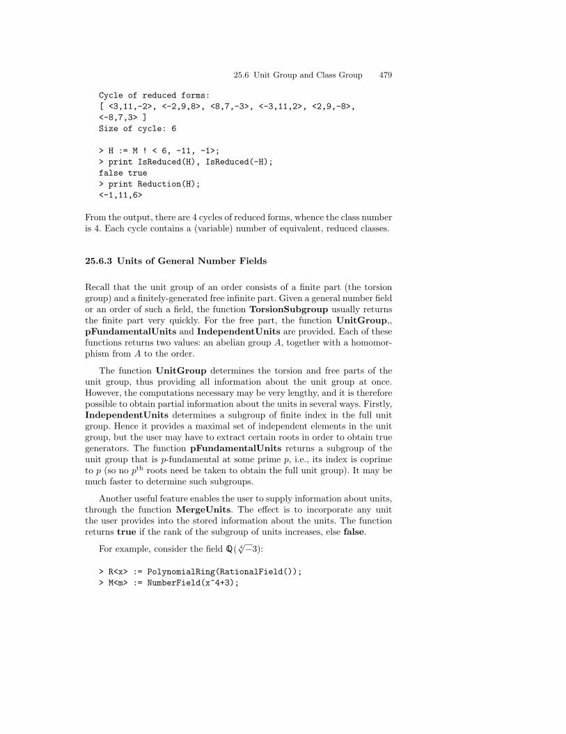
25.6 Unit Group and Class Group 479
Cycle of reduced forms:[ <3,11,-2>, <-2,9,8>, <8,7,-3>, <-3,11,2>, <2,9,-8>,<-8,7,3> ]Size of cycle: 6
> H := M ! < 6, -11, -1>;> print IsReduced(H), IsReduced(-H);false true> print Reduction(H);<-1,11,6>
From the output, there are 4 cycles of reduced forms, whence the class numberis 4. Each cycle contains a (variable) number of equivalent, reduced classes.
25.6.3 Units of General Number Fields
Recall that the unit group of an order consists of a finite part (the torsiongroup) and a finitely-generated free infinite part. Given a general number fieldor an order of such a field, the function TorsionSubgroup usually returnsthe finite part very quickly. For the free part, the function UnitGroup,,pFundamentalUnits and IndependentUnits are provided. Each of thesefunctions returns two values: an abelian group A, together with a homomor-phism from A to the order.
The function UnitGroup determines the torsion and free parts of theunit group, thus providing all information about the unit group at once.However, the computations necessary may be very lengthy, and it is thereforepossible to obtain partial information about the units in several ways. Firstly,IndependentUnits determines a subgroup of finite index in the full unitgroup. Hence it provides a maximal set of independent elements in the unitgroup, but the user may have to extract certain roots in order to obtain truegenerators. The function pFundamentalUnits returns a subgroup of theunit group that is p-fundamental at some prime p, i.e., its index is coprimeto p (so no pth roots need be taken to obtain the full unit group). It may bemuch faster to determine such subgroups.
Another useful feature enables the user to supply information about units,through the function MergeUnits. The effect is to incorporate any unitthe user provides into the stored information about the units. The functionreturns true if the rank of the subgroup of units increases, else false.
For example, consider the field Q( 4√−3):
> R<x> := PolynomialRing(RationalField());> M<m> := NumberField(x^4+3);

480 25. Number Fields
> T, t := TorsionSubgroup(M);> print T;Abelian Group isomorphic to Z/6Defined on 1 generatorRelations:
6*T.1 = 0> print t(T.1);[1, 0, 1, 0]> u0 := M ! t(T.1);> print u0;1/2*m^2 + 1/2> print UnitRank(M);1
From the output, the ring of integers of M (which has not been created ex-plicitly!) contains only the (expected) sixth roots of unity, namely the powersof (
√−3 + 1)/2. It is also now known that one free generator is required. Inthe next lines, a unit is found, and used to extend the known subgroup:
> print <a, b> : a, b in [-5..5] | Norm(m^2+a*m+b) eq 1 ; <-2, 2>, <2, 2> > print MergeUnits(M, m^2-2*m+2);true> I, i := IndependentUnits(M);> u1 := M ! i(I.2);> print u1;m^2 - 2*m + 2
This furnishes independent units. Now the 2-fundamental part of the unitgroup and the full unit group are determined:
> V, v := pFundamentalUnits(M, 2);> u2 := M ! v(V.2);> print u2;-1/2*m^3 + 1/2*m - 1> U, u := UnitGroup(M);> u3 := M ! u(U.2);> print u3;1/2*m^3 - 1/2*m^2 + 1/2*m + 1/2
It emerges that the group V was the full unit group already, since u2 and u3differ by a root of unity, and that the subgroup I was of index 2:
> tU := u0^i : i in [1..6] ; // roots of unity in M> print u3*u2^-1 in tU;

25.6 Unit Group and Class Group 481
true> print u3*u1^-1 in tU;false> print Logs(u1), Logs(u3);[ -1.6628858910586214, 1.6628858910586211 ][ -0.8314429455293105317, 0.83144294552931051793 ]> print u3^2*u1^-1 in tU;true;
If only the regulator of an order is required, Regulator can be invoked. Thisfunction will trigger the computation of units (and of the maximal order) ifnecessary.
The table lists the real-valued functions we mentioned, and some others.
Table 25.15. Some real-valued functions
Magma Meaning
Regulator(O) Regulator of order O
Conjugates(a) Sequence of conjugates of a as complex numbers
Conjugate(a, k) kth term of above sequence
AbsoluteValues(a) Sequence of absolute values of conjugates of a, as realnumbers
Logs(a) Sequence of logarithms of absolute values of conjugatesof a, as real numbers
Length(a) T2 norm of a
Zeros(O, n) Zeros of defining polynomial of O up to precision atleast n
There is another way the user may supply information to Magma inorder to avoid expensive computation. The functions SetOrderMaximal,SetOrderUnitsAreFundamental, and SetOrderTorsionUnits may beused to set flags indicating that an order is maximal, or that the units foundso far are fundamental, or to supply all torsion units.
Magma also provides a function to calculate exceptional units and todetermine S-units and S-class groups. See the Handbook.
25.6.4 Class Groups of General Number Fields
Fractional ideals, under equivalence up to multiplication by principal ideals,form a group known as the ideal class group of the order. In Magma, classgroup computations for general number fields are restricted to the maximal

482 25. Number Fields
order of the field. The main method employed to determine the ideal classgroup of the maximal order is the relation method. It can be briefly describedas follows.
In the first step a list of prime ideals is generated, all having norm belowsome given bound. This is the factor basis. In the second step a search isconducted to find a few elements in each of these prime ideals such thatthe principal ideal generated factors completely over the factor basis. Theseprovide relations between the ideals in the factor basis, and from them, abasis for the class group is determined. Finally, it is checked that the correctorders for the basis elements are found. Here knowledge about units in theorder is required.
Table 25.16. Class group functions for general number fields
Magma Meaning
MinkowskiBound(K) Minkowski bound for K
BachBound(K) Bach bound for K
FactorBasis(K, b) Factor basis of primes of norm below b inmaximal order of K
RelationMatrix(K, b, n) Matrix representing n relations for eachideal in factor basis with bound b over max-imal order of K
To obtain results that are guaranteed to be correct, the factor basis needsto contain all prime ideals below the Minkowski bound; assuming certainRiemann hypotheses the (usually much lower) Bach bound may be used. Forboth values a function is provided, as listed in Table 25.16. The functionsFactorBasis and RelationMatrix allow the user to generate the necessaryrelation matrix, after which matrix functions can be used to complete therelation algorithm. (All these functions can take the maximal order as analternative to the field.)
The functions ClassNumber, ClassGroupStructure and ClassGroupprovide a complete implementation of the method. They differ in the formof the output, yielding the mere cardinality of the group, the structure ofthe abelian group, and the group itself, respectively. (As its second returnvalue, ClassGroup provides a mapping from the abelian group to the setof ideals.) In the default version all three take just a general number fieldas their argument (the maximal order is allowed as substitute for the field).The default version uses the Minkowski bound and executes the complete re-lation method. In practice, for even moderately sized fields, this takes a verylong time to finish. Moreover, with a much smaller bound correct results willusually be obtained, in a reasonable time. By means of parameters, the user

25.6 Unit Group and Class Group 483
can instruct Magma to employ such a modified method. The most impor-tant parameters are Bound (for an alternative to the Minkowski bound) andCheck, which, when set to false, instructs Magma not to perform poten-tially expensive checks at the end of the algorithm. It needs to be stressedthat the use of these parameters may invalidate the results: if the bound istoo small, it may be that only a subset of the generators is used (and hencethe result will be too small), whereas omitting the check at the end may meanthat not all relations are found and that the result is too large.
A typical example is given below:
> N<n> := NumberField(x^8 - 15);> C, h := ClassGroup(N : Bound := 1000, Check := false);> print C;Abelian Group isomorphic to Z/4 + Z/4Defined on 2 generatorsRelations:
4*C.1 = 04*C.2 = 0


26. The Real and Complex Fields
Section 3.5 provided a brief introduction to real and complex numbers inMagma. This chapter explains how to calculate in a real field or complexfield. By the nature of IR and C, the real and complex fields constructed byMagma are different from most other Magma fields: computation in themis not exact, only approximate. Therefore these ‘fields’ are not true fields; infact, they are not even commutative rings. However, Magma’s algorithmsfor real and complex arithmetic have been designed to produce results thatare accurate within whatever precision is chosen by the user.
26.1 The Two Kinds of Real and Complex Fields
There are two kinds of real fields in Magma: free fields and fields of fixedprecision. In the free real field, each element has its own relative precision,which may be as high as the user specifies, or else infinite (for integers andrationals considered as exact reals). Magma’s implementation of these fieldsis based on the PARI package. On the other hand, in a fixed precision realfield every element of the field has the same precision, which once again maybe arbitrarily high. Magma’s implementation of fixed precision fields is basedon R. P. Brent’s MP-package.
There are also two kinds of complex fields. The elements of the free com-plex field have real and imaginary parts which are each members of a freereal field. The real and imaginary parts may have different relative precisions,and the overall relative precision of the element is the smaller of the two. Bycontrast, the elements of a fixed precision complex field of precision p havereal and imaginary parts which are each members of a fixed precision realfield of the same precision p.
The functions for creating these fields are RealField and ComplexField.For the free real and complex fields, the function takes no arguments, but fora fixed precision real or complex field, it takes a precision p as its argument:
> R := RealField();

486 26. The Real and Complex Fields
> print R, Category(R);Real FieldFldPr> R32 := RealField(32);> print R32, Category(R32);Real Field of precision 32FldRe> C<i> := ComplexField();> print C, Category(C);Complex FieldFldPr> C32<j> := ComplexField(32);> print C32, Category(C32);Complex Field of precision 32FldCom
When a complex field is created, the angle bracket notation (generator as-signment) is the best way of giving the element
√−1 the special name i (orj, or any other chosen name).
Given a fixed precision field, the function Precision returns its precision.For instance:
> print Precision(R32), Precision(C32);32 32
26.2 Working in the Default Real Field
For many purposes, it is sufficient to know how to work within the default realfield, that is, the real field which Magma uses unless there is an instructionto the contrary. The notation i.j, where i and j are each a succession ofdecimal digits, always creates the corresponding real number as an elementof the default real field. For example:
> a := -18.394;> print Parent(a);Real Field
This assigns the real number −18.394 to the identifier a. The parent of a willbe the default real field, which in this case is the free field.
Scientific notation should be used in order to express very large or verysmall real numbers. Immediately after the decimal number i.j the user may

26.2 Working in the Default Real Field 487
put e followed by an integer s. Magma evaluates this as the real numberwhich is i.j×10s. For instance, the following line assigns to b the real number901.2× 10−14:
> b := 901.2e-14;
Again, the parent of this element will be the default real field.
It is sometimes useful to go in the other direction, that is, to express areal number x as m · 10e, where m is a real number and e is an integer. Thefunction MantissaExponent(x) returns both these values, but since thereare an infinite number of correct responses, it returns m and e such that1 ≤ m < 10:
> mant, exp := MantissaExponent(b);> print mant, exp;9.0119999999999999999999999998481 -12
The output indicates that b equals 9.012×10⁻¹². (The trailing 9’s in the out-put should not be a matter for concern. They often arise as the consequenceof converting from the internal base to which free reals are stored.)
The concept of relative precision is based on the concept of mantissaand exponent. The relative precision of a real number x, returned byPrecision(x), is the number of significant decimal digits in the mantissa.For instance, b and mant must have the same relative precision:
> print Precision(b);28> print Precision(mant);28
The next section explains why the relative precision of these numbers is 28.
When Magma starts up, the default real field is the free field. The fol-lowing example demonstrates how to obtain the current default, and how toreset it:
> print GetDefaultRealField();Real Field> SetDefaultRealField(RealField(48));> print GetDefaultRealField();Real Field of precision 48> print Parent(a);Real Field> c := 1.4;

488 26. The Real and Complex Fields
> print Parent(c);Real Field of precision 48
Notice that a change in the default real field does not change the parent ofelements that already exist.
This chapter contains many functions that take a real number as an ar-gument and return a real number. Whether the parent of the return valueis a free field or fixed precision field depends on the parent of the input. Forinstance:
> print Parent(Sin(a));Real Field> print Parent(Sin(c));Real Field of precision 48
However, these functions often accept other categories of input (such as in-tegers, rationals, quadratic field elements and cyclotomic field elements) ifthe input can be coerced into a real number. If this is possible, the input iscoerced into the default real field, so the output will also belong to that field.For instance, the current default real field in the example is the real field offixed precision 48. When a real function is applied to a rational number, therational is coerced automatically into that field, and the return value willbelong to it too:
> print Parent(Sin(3/4));Real Field of precision 48
The rules for free fields and fixed precision fields are explained in thefollowing sections.
26.3 The Free Real Field
In the examples of this section it will be assumed that the default real fieldhas been set to the free real field (as is the case at the beginning of a Magmasession). The following command ensures that this is true:
> SetDefaultRealField(RealField());
In the free field, a real number may be created with a relative precision ofarbitrary size (within reason). If the real number has a precision greater than28 (or the current default precision), it may be typed directly, as explainedabove. Magma will automatically provide sufficient precision to store everydigit of the number. For example:

26.3 The Free Real Field 489
> d := 1.23456789012345678901234567890123456789012345678e22;> print d;12345678901234567890123.456789012345678901234567793305> print Precision(d);48
If the mantissa of the number ends with many trailing but significantzeros, it can be inconvenient to type them all. However, omitting the zerosgives a different result:
> f1 := 5.5550000000000000000000000000000000000e6;> print Precision(f1);38> f2 := 5.555e6;> print Precision(f2);28
The solution to this problem is to follow the real number immediately by pand the desired precision:
> f3 := 5.555e6p38;> print Precision(f3);38
Not every integer may be used internally as a precision, because of theway that Magma stores these numbers. Therefore Magma will sometimesincrease the requested precision slightly. This should not cause any majordifficulties. For example:
> print Precision(7.9p50), Precision(7.9p80);57 86
If no precision is given and the number of digits in the mantissa is smallerthan 28 (or the current default precision), then Magma will choose 28 as theprecision rather than the number of mantissa digits. This is what happenedin the calculation of f2 , above. In order to override this, the desired precisionmust be specified using p:
> f4 := 5.555e6p9;> print Precision(f4);9
The free real field can also contain exact elements. They are created whenan integer or rational is coerced into the field. The relative precision of anexact real is infinity, but Magma represents it as −1. For instance:

490 26. The Real and Complex Fields
> f5 := R!(22/7); print f5;22/7> print Parent(f5);Real Field> print Precision(f5);-1
The discussion above included several instances where the free field makesuse of the number 28. This number is the default value of the default precisionattribute for the free field. If the user finds that 28 is an unsuitable defaultvalue for this attribute, then the value should be changed. It is returned andaltered by the function HasAttribute and the procedure AssertAttribute.These intrinsics are used in several contexts within Magma. When they areused with reference to the default precision attribute of the free field, thefirst argument must be the category of the free field, FldPr, and the secondargument must be the string "Precision". AssertAttribute takes a thirdargument, the new default precision. The function HasAttribute returnstwo values: a Boolean specifying whether the attribute is defined (this willalways be true in this case, so it can be ignored); and the current value ofthe attribute. For example:
> print HasAttribute(FldPr, "Precision");true 28> AssertAttribute(FldPr, "Precision", 57);> print HasAttribute(FldPr, "Precision");true 57> print Precision(f2);28> print Precision(7.9);57
Note carefully that the change to the attribute does not affect the precisionof previously existing elements of the free real field. For elements createdafter the change in attribute, the new attribute value (57 in this example)will behave in exactly the same way as 28 did before.
One of the applications of the default precision attribute is to state theprecision when an object that is not an element of the free real field R iscoerced into R. This can happen as an explicit coercion:
> Qu3<rt3> := QuadraticField(3);> print R!rt3;1.7320508075688772935274463415058723669428052538103806280556> print Precision(R!rt3);57

26.4 The Fixed Precision Real Fields 491
or when a real function accepts several categories of input (e.g., reals, integers,rationals) but coerces the input into the free real field before performing theoperation:
> print Exp(30);10686474581524.46214699046865074140165002449500547305499022\24923> print Precision(Exp(30));57
(The above example has been calculated using the free real field as the defaultfield.)
26.4 The Fixed Precision Real Fields
In a fixed precision real field, every real number in the field has the sameprecision. The function RealField(p) returns the real field of fixed precisionp. More precisely, although any positive integer may be given as the precision,Magma always rounds the input up to the nearest multiple of 4 to find theprecision, because it stores elements of fixed precision real fields internally toa base of 104. For instance, a request for a precision of 29 or 30 or 31 willresult in a precision of 32, just as if the user had requested that precisiondirectly.
Before working within a real field R of fixed precision p, it is ad-visable to make that field into the default real field, with the functionSetDefaultRealField(R). (The resulting value may be checked with thefunction GetDefaultRealField().) For instance, the instruction used tospecify a real field of precision 16 is:
> SetDefaultRealField(RealField(16));> print GetDefaultRealField();Real Field of precision 16
After the default field has been set in this way, every input of the form i.j ori.jes will produce a member of this field, with that precision:
> g1 := 3.893276e-217;> print g1;3.893276e-217> print Parent(g1);Real Field of precision 16> g2 := 1234.567812345678123456781234567812354678;

492 26. The Real and Complex Fields
> // NB: some digits are lost> print g2;1234.567812345678> print Precision(g2);16
It is important to realize that the interpretation of the p notation dependson the current category of default real field. If the default field is the free field,then p means to create a free field element with an unusual precision; thiswas demonstrated in the previous section. If the default field is one of thefixed precision fields, then p indicates a request to create an element in a fieldof given fixed precision, rather than in the default field. For example, if thedefault field is the field of precision 16, then the p notation may be used tocreate a real number of some other precision, as an element of another fixedprecision field:
> g3 := 1234.567812345678123456781234567812354678p60;> print g3;1234.567812345678123456781234567812354678> print Precision(g3);60> print Parent(g3);Real Field of precision 60
It is only approximately true that the precision of fixed precision reals isthe same as the number of significant figures in decimal form. The truth isa little more complicated. Since the digits on the left and right sides of thedecimal point are stored separately, every block or part-block of 4 digits oneach side requires 4 digits of precision. The following example demonstratesthis:
> print 61532.61437p8;61533> print 61532.61437p12;61532.6144> print 61532.61437p16;61532.61437
In this example, the part on the left of the decimal point in 61532.61437consists of 5 digits, so 8 precision digits are required to store it. In the firststatement, since only 8 digits are available, Magma evaluates only this leftpart, rounded up because the part on the right of the decimal point is notless than a half. In the second example, the 12 precision digits are used torepresent the left part and the first four digits of the right part, roundedonce again. In the last example, there are sufficient digits for the complete

26.4 The Fixed Precision Real Fields 493
number. It follows that to store a fixed precision real number successfully,the precision must be set at least 6 digits higher than the required numberof significant figures.
Many kinds of ring elements may be coerced into a fixed precision realfield. For example:
> Qu5<rt5> := QuadraticField(5);> print RealField(52)!(2 + 3*rt5);8.708203932499369089227521006193828706321855078836> print 2 + 3*Sqrt(5p52); // comparison8.708203932499369089227521006193828706321855078836
Coercion may also be used to convert a real number into the equivalentnumber with a different precision, by coercing it into the appropriate fixedprecision real field. If the new precision is less than the old precision, thenrounding will occur if necessary, and if the new precision is greater thanthe old precision, the number is padded with trailing zeros until the requiredprecision is reached. (Consequently, once the precision of a number is reduced,the ‘lost’ digits can never be regained by coercing into a higher precision.)For example:
> rt3 := Sqrt(3.0p12); print rt3;1.73205081> rt3prec8 := RealField(8)!rt3; print rt3prec8;1.7321> rt3prec48 := RealField(48)!rt3; print rt3prec48;1.73205081> print RealField(100)!rt3prec8;1.7321
The e and p notations are limited to contexts where the exponent andprecision are known as literals. In situations where they are only known asexpressions, such as in the course of a function, the elt constructor shouldbe used instead:
elt< RealField(p) | t, s >
This constructor creates the real number t · 10s of precision p, where t is anexpression coercible into a real, and p and s are integer-valued expressions.(The user should be careful about the precision of t, if it is given as a realliteral in the default real field, to ensure that the result is sufficiently precise.)The following example shows how to express the number 42
9 × 10⁷ as anelement of the real field of fixed precision given by the identifier prec:
> prec := 52;
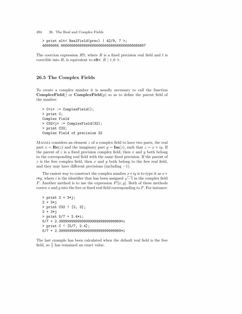
494 26. The Real and Complex Fields
> print elt< RealField(prec) | 42/9, 7 >;46666666.66666666666666666666666666666666666666667
The coercion expression R!t, where R is a fixed precision real field and t iscoercible into R, is equivalent to elt< R | t, 0 >.
26.5 The Complex Fields
To create a complex number it is usually necessary to call the functionComplexField() or ComplexField(p) so as to define the parent field ofthe number:
> C<i> := ComplexField();> print C;Complex Field> C32<j> := ComplexField(32);> print C32;Complex Field of precision 32
Magma considers an element z of a complex field to have two parts, the realpart x = Re(z) and the imaginary part y = Im(z), such that z = x + iy. Ifthe parent of z is a fixed precision complex field, then x and y both belongto the corresponding real field with the same fixed precision. If the parent ofz is the free complex field, then x and y both belong to the free real field,and they may have different precisions (including −1).
The easiest way to construct the complex number x+iy is to type it as x+i*y, where i is the identifier that has been assigned
√−1 in the complex fieldF . Another method is to use the expression F ![x, y]. Both of these methodscoerce x and y into the free or fixed real field corresponding to F . For instance:
> print 2 + 3*j;2 + 3*j> print C32 ! [2, 3];2 + 3*j> print 5/7 + 2.4*i;5/7 + 2.399999999999999999999999999969*i> print C ! [5/7, 2.4];5/7 + 2.399999999999999999999999999969*i
The last example has been calculated when the default real field is the freefield, so 5
7 has remained an exact value.

26.6 Elementary Real and Complex Operations 495
Another way of creating a complex number is to give its polar coordinates.The function PolarToComplex(m, a) returns the complex number meai =m(cos a+ i sin a). To make use of this function, the function Pi(R) is helpful;it returns π to the same precision as the real field R. Therefore a numbersuch as 8(cos(π
6 ) + i sin(π6 )) may be created in the following way:
> pi := Pi(R32); print pi;3.1415926535897932384626433833> print PolarToComplex(8, pi/6);6.928203230275509174109785366 + 4*j
Within the precision, the result equals 4√
3 + 4j.
Coercion into a complex field works in the same way as coercion into a realfield. Note that all elements of quadratic and cyclotomic fields are coercibleinto a complex field, whereas only some of them (those with zero imaginaryparts) are coercible into a real field:
> Q7<sev> := CyclotomicField(7);> print C ! sev;0.62348980185873353052500488400+ 0.781831482468029808708444526665775860168*i
26.6 Elementary Real and Complex Operations
Table 26.1. Elementary real-number functions
Magma Meaning
Abs(r) Absolute value |r| of r
Norm(r) |r| if r is a fixed precision real, else |r|2Sign(r) Returns −1, 0, or 1 depending on whether r is negative,
zero, or positive respectively
Sqrt(r) Square root of non-negative real r
Root(r, n) nth root of r, if a real root exists
Floor(r) The greatest integer brc less than or equal to r
Ceiling(r) The smallest integer dre greater than or equal to r
Round(r) The integer nearest r (n+ 12
is rounded to n+1, for n ∈ ZZ)
Truncate(r) The integer part of r, or r rounded towards zero, i.e.,Sign(r)*b |r| c

496 26. The Real and Complex Fields
Table 26.2. Elementary complex-number functions
Magma Meaning
Re(c),Real(c) Real part of c
Im(c), Imaginary(c) Imaginary part of c
IsReal(c) true if Im(c) is zero
IsIntegral(c) true if Im(c) is zero and Re(c) is an integer
PolarToComplex(m, a) Complex number c = meia, with modulus m andargument a
ComplexToPolar(c) Returns modulus m and principal argument a of csuch that c = meia
Modulus(c) |c|Arg(c),Argument(c) Principal argument of c, in radians
Norm(c) |c|2ComplexConjugate(c) Complex conjugate x− yi of c = x + yi
Sqrt(c) Square root of c
The operations of elementary arithmetic on real and complex numbers canbe performed using the usual Magma operators. There are also the functionsZero(F ) and One(F ), which return the 0 and 1 of a real or complex fieldF . If a binary operation is performed on a combination of a real/complexnumber and an object coercible into a real/complex field, then Magma willautomatically coerce the second object into a suitable field, with appropriateprecision.
The customary Boolean functions for field elements apply to the real andcomplex fields: IsZero(a), IsOne(a), and IsMinusOne(a). The operatorseq and ne and all the membership operators can also be used in both the realfields and the complex fields. The ordering operators such as lt are applicableto the real fields but not the complex fields, since ordering is not a propertyof the complex field. All of these Boolean tests examine the number as itis, with its given precision; that is, they require the test to hold within theprecision of the argument(s).
The functions PolarToComplex(m, a) and ComplexToPolar(c) areinverses, in a sense: the first takes the modulus and argument of a complexnumber and returns the number, and the second takes the number and returnsthe modulus and argument. These values may also be obtained separately,from the functions Modulus(c) and Arg(c) (or Argument(c)). Since theidentity meia = mei(a+2πk) for all k ∈ ZZ poses an ambiguity for Arg(c), thevalue a that is returned is the principal argument, i.e., the value satisfying−π < a ≤ π.
Table 26.1 and Table 26.2 (p. 496) list the elementary functions on realand complex numbers.

26.7 Standard Real Constants 497
26.7 Standard Real Constants
Three functions return standard real constants, to the precision of a givenreal or complex field F . If F is complex then the return value is a complexnumber whose imaginary part is zero and whose real part approximates theconstant. The most important of these functions is Pi(F ):
> print Pi(RealField(28));3.141592653589793238462643
The other two functions are EulerGamma(F ), which returns Euler’s Γconstant, and Catalan(F ), which returns Catalan’s constant, the sum givenby
∑∞k=0(−1)k(2k + 1)−2:
> print EulerGamma(R);0.57721566490153286060651209008> print Catalan(RealField(52));0.9159655941772190150546035149323841107741493742816721
26.8 Advanced Real and Complex Functions
The functions in this section return results with the same precision as theprecision of the arguments. Most of them accept both real and complex input,from either kind of field, but in some cases only elements of the free fieldsare accepted. If the function is given integer or rational arguments, then thereturn value will belong to the default real field (or its complex version).
These functions are designed to be fast, numerically stable, and accurateto the very last digit.
26.8.1 Transcendental Functions
Given a real or complex number c, Exp(c) returns ec, the exponential func-tion of c. The inverse function, Log(c), returns loge c. Moreover, Log(b, c)calculates logb c, the logarithm of c to the base b. For instance:
> print Exp(1p48);2.7182818284590452353602874713526624977572470936977> print Log(10);2.302585092994045684017991454658> print Log(10, 1000);3.0000000000000000000000000000

498 26. The Real and Complex Fields
Table 26.3. Exponential and logarithmic functions
Magma Meaning
Exp(c) Exponential ec of c
Log(c) Principal value of logarithm of c to base e
Log(b, c) Logarithm of c to real base b
Dilog(c) Principal value of dilogarithm Li2(c)
Polylog(m, c) Principal value of polylogarithm Lim(c)
PolylogD(m, c) Principal value of modified version Dm of Lim(c)
PolylogDold(m, c) Principal value of modified version Dm of Lim(c)
PolylogP(m, c) Principal value of modified version Pm of Lim(c)
Table 26.3 lists these and other logarithmic functions.
26.8.2 Trigonometric and Hyperbolic Functions
Table 26.4. Trigonometric and hyperbolic functions
Sin(c) Arcsin(c) Sinh(c) Argsinh(c)
Cos(c) Arccos(c) Cosh(c) Argcosh(c)
Tan(c) Arctan(c) Tanh(c) Argtanh(c)
Cosec(c) Arccosec(c) Cosech(c) Argcosech(c)
Sec(c) Arcsec(c) Sech(c) Argsech(c)
Cot(c) Arccot(c) Coth(c) Argcoth(c)
Sincos(c) Arctan2(b, a)
As shown in Table 26.4, Magma provides the full range of trigonometricand hyperbolic functions such as Sin and Sinh, together with their inversessuch as Arcsin and Argsinh. The only two functions whose meanings arenot immediately apparent are Sincos and Arctan2. Sincos(c) returns twovalues, the sine and the cosine of c. Arctan2(b, a) returns a number whosetangent is b
a and which is in the quadrant indicated by the signs of b and a.
The angles are measured in radians, so to calculate in degrees it is neces-sary to multiply by the conversion factor π
180 :
> DegToRad := Pi(RealField(20)) / 180; print DegToRad;0.01745329251994329556> print Sin(30 * DegToRad);0.49999999999999999456> print Cos(45 * DegToRad);

26.8 Advanced Real and Complex Functions 499
0.7071067811865475310
The examples indicate that sin 30 = 12 and cos 45 = 1√
2. The answers are
not exact, since DegToRad does not equal π180 to infinite precision.
The inverse trigonometric functions return values in the customary ranges,that is, 0 to π for Arccos and Arcsec, and −π
2 to π2 for the other four.
26.8.3 Summation of Infinite Series
Magma includes functions for evaluating infinite sums: InfiniteSum(m, i),PositiveSum(m, i), and AlternatingSum(m, i). Here m is a map from theintegers to the free real field, such that m(n) is the nth term of the sum. Thesummation starts at term i, where i is a non-negative integer.
Each of the three functions returns essentially the same result. The firstof them, InfiniteSum, simply evaluates successive terms of the series andadds them together, until the result is within the default precision of thefree real field. The other two functions employ special techniques to do thismore effectively: PositiveSum is designed for series in which every termis positive, and AlternatingSum is designed for series in which the termsalternate in sign.
For example, consider the series
π
4= 1− 1
3+
15− 1
7+ · · ·
ande = 1 +
12!
+13!
+ · · ·They may be verified as follows:
> Z := IntegerRing();> R := RealField();> AssertAttribute(FldPr, "Precision", 57);> m := map< Z -> R | n :-> (-1)^n / (2*n+1) >;> print Pi(R)/4 - AlternatingSum(m, 0);1.5930919107 E-58
> f := map< Z -> R | n :-> 1/Factorial(n) >;> print Exp(1) - InfiniteSum(f, 0);-4.3769182618 E-58

500 26. The Real and Complex Fields
26.8.4 Continued Fractions
Magma provides several functions for continued fractions. Given a free realnumber r, ContinuedFraction(r) returns the partial quotients in the con-tinued fraction expansion of r, as a sequence of integers. As many partialquotients will be given as the precision of r permits. For example:
> pi := Pi(RealField());> cf := ContinuedFraction(pi);> print cf;[ 3, 7, 15, 1, 292, 1, 1, 1, 2, 1, 3, 1, 14, 2,1, 1, 2, 2, 2, 2, 1, 84, 2, 1, 1, 15, 3 ]
The function BestApproximation(r, n) returns the best rational ap-proximation to r with denominator not exceeding n. This calculation is madeusing continued fraction techniques. Continuing the example:
> print BestApproximation(pi, 10);22/7> print BestApproximation(pi, 130);355/113> print 355/113 - pi;0.000000266764189062422312368998957356
Finally, Convergents(Q) returns the convergents matrix of the integersequence Q, where Q is interpreted as a sequence of partial quotients. Thismatrix is a 2 × 2 integer matrix m such that m12/m22 and m11/m21 formthe last two convergents for r as provided by Q. For instance:
> cv := Convergents(cf);> print cv;[428224593349304 139755218526789][136308121570117 44485467702853]> print cv[1,2]/cv[2,2] - pi;1.9965585740 E-28> print cv[1,1]/cv[2,1] - pi;5.21276888810 E-29
26.8.5 Special Functions
Table 26.5 (p. 501) shows Magma’s intrinsics for some other standard realfunctions. Many of them are available for elements of the free field only.

26.8 Advanced Real and Complex Functions 501
Table 26.5. Special functions
Magma Meaning
JacobiTheta(q, z) First Jacobi θ function θ(q, z)
JacobiThetaNull(q, k) kth derivative of θ(q, z) at z = 0
DedekindEta(c) Dedekind’s function η(c)
jInvariant(c) Elliptical j-invariant j(c)
WeberF(c) Weber’s function f(c)
WeberF2(c) Weber’s function f2(c)
Gamma(c) Γ (c)
Gamma(x, y) Incomplete γ function γ(x, y)
GammaD(c) Γ (c + 12)
LogGamma(c) Principal value of log Γ (c)
LogDerivative(c),Psi(c) Principal value of Ψ(c) = d log Γ (c)dc
BesselFunction(n, r) Bessel function of the 1st kind Jn(r), wherer is in a fixed precision real field
JBessel(n, r) Bessel function of the 1st kind of 12-integral
index Jn+ 12(r), where r is in a free real field
KBessel(n, r) Modified Bessel function of the 2nd kindKn(r)
KBessel2(n, r) Another implementation of KBessel(n, r)
HypergeometricU(a, b, r) Confluent hypergeometric fn U(a, b, r)
AGM(c, d) Arithmetic-geometric mean of c and d
BernoulliNumber(n) nth Bernoulli number Bn, as a rational
BernoulliApproximation(n) Approximation to Bn, as a finite-precisionfree real
DawsonIntegral(r) Dawson’s integral at r
ErrorFunction(r),Erf(r) Error function erf(r)
Erfc(r) Complementary error function 1 − erf(r)
ExponentialIntegral(r) Exponential integral ei(r)
LogIntegral(r) Logarithmic integral li(r)
ZetaFunction(c) Riemann ζ function ζ(c), for c in free field
ZetaFunction(R, n) Riemann ζ function ζ(n) for integer n 6= 1,evaluated in fixed precision real field R
As an example, consider the beta function B(r, s). Magma does not havea function for B(r, s), but it is related to the gamma function by
B(r, s) =Γ (r)Γ (s)Γ (r + s)
so a user-defined function BetaFunction(r, s) may be defined as follows:
> BetaFunction := func< r, s |> Exp(LG(r) + LG(s) - LG(r+s)) where LG is LogGamma>;

502 26. The Real and Complex Fields
The function could be defined using Gamma rather than LogGamma, butLogGamma is preferable since Gamma is a rapidly increasing function.
26.8.6 Example: The Prime Number Theorem
The prime number theorem states that π(n)
li(n)→ 1 as n →∞, where π(n) is the
number of primes less than or equal to n and li(n) is the logarithmic integralof n. Riemann extended the prime number theorem by defining a functionR(n) =
∑∞k=1
µ(k)k li( k
√n), where µ(n) is the Mobius µ function, which also
tends asymptotically to π(n) but at a faster rate. (The first term of the sumis the simple approximation li(n).)
The following procedure prints statistics of the prime number theorem upto a given limit. For n =10, 100, 1000, . . . such that n ≤ limit , it prints
n, π(n), li(n),π(n)li(n)
, R(n),π(n)R(n)
.
In their printed version only, li(n) and R(n) are rounded to the nearest inte-ger. The identifiers for this procedure are as follows: final prime stores thegreatest prime ≤ n; true c stores the number of primes ≤ n; li c stores theli(n) approximation to true c; and rie c stores the Riemann approximationR(n) (summing the first 15 terms only) to true c.
To perform this example online, type load "I96c26e1";
PrimeNumberTheorem := procedure(limit)n := 10;final_prime := 7;true_c := 4;// fields of lower precision than the default,// used for convenience of printingR8 := RealField(8);R4 := RealField(4);
// the heading for the outputprint "n\tpi(n)\tli(n)\tpi(n)/li(n)\tR(n)\tpi(n)/R(n)";print "-"^58;
while n le limit dop := NextPrime(final_prime);while p le n do
true_c +:= 1;final_prime := p;p := NextPrime(final_prime);
end while;li_c := LogIntegral(R8!n);

26.8 Advanced Real and Complex Functions 503
true_li := true_c / li_c;rie_c :=
&+[LogIntegral(Root(R8!n, k)) * MoebiusMu(k)/k :k in [1..15]];
true_rie := true_c / rie_c;printf "%o\t%o\t%o\t%o\t\t%o\t%o\n",
n, true_c,Round(li_c), (true_li lt 1 select R4 else R8)!true_li,Round(rie_c), (true_rie lt 1 select R4 else R8)!true_rie;
n *:= 10;end while;
end procedure;
A suitable call to this procedure would be:
> PrimeNumberTheorem(1000000);n pi(n) li(n) pi(n)/li(n) R(n) pi(n)/R(n)----------------------------------------------------------10 4 6 0.6488 4 0.8911100 25 30 0.8299 26 0.97521000 168 178 0.9459 168 0.997810000 1229 1246 0.9863 1227 1.0017100000 9592 9630 0.9961 9587 1.00051000000 78498 78626 0.9984 78525 0.9997


Part VI
Modules and Algebras


27. Vector Spaces and Matrix Spaces
The most general kind of module which can be constructed in Magma is amodule of dimension n over a ring R. Magma offers two ways of viewing suchstructures: as (R-)tuple spaces with an embedded basis, or as (R-)moduleswith a reduced basis. This chapter discusses the former view only.
If the ring over which a tuple space is defined is a field K, then thestructure which emerges is a K-space, more commonly known as a (finitely-generated) vector space. Its elements are row vectors. The category of suchstructures in Magma is ModTupFld. (The field K must be defined as amember of a Fld category, so that Magma knows it is a field.) For the sakeof clarity and familiarity, this chapter concentrates on vector spaces, althoughmost of the operations are also available for R-spaces, that is, tuple spacesover a general ring R (category ModTupRng).
A further topic of this chapter is matrix spaces. Again, the emphasiswill be on K-matrix spaces (ModMatFld), but the operations for R-matrixspaces in general (ModMatRng) closely resemble them. The elements ofmatrix spaces are represented as rectangular matrices, and may be consideredeither as vector-like objects printed as matrices, or as homomorphisms fromone vector space to another.
27.1 Constructing the Full Vector Space
Every vector space of finite dimension n over a field K is isomorphic to thevector space K(n), that is, the space of n–dimensional coordinates whoseentries are elements of K. This space is known as the full vector space.It may be created in Magma using the function VectorSpace(K, n), orKSpace(K,n). For example, the full 5–dimensional vector space over therational field Q may be constructed as follows:
> Q := RationalField();> V5 := VectorSpace(Q, 5);

508 27. Vector Spaces and Matrix Spaces
It is not necessary to assign the field to an identifier before creating thevector space. Thus the following line will create the 3–dimensional vectorspace V3F11 over the finite field with eleven elements:
> V3F11 := VectorSpace(GF(11), 3);
The function Basis(V ) returns the basis of a vector space V . If V is afull vector space, then it returns the standard basis, in which the ith basisvector is the vector that has the identity of the field K as its ith entry, andthe zero of K in all other coordinate positions. For example:
> print V3F11;Full Vector space of degree 3 over GF(11)> print Basis(V3F11);[
( 1 0 0),( 0 1 0),( 0 0 1)
]
For full vector spaces created using VectorSpace(K), the generators are thesame as the basis vectors, and the ith generator, V .i, is the ith basis vector:
> print Generators(V3F11);
( 0 1 0),( 1 0 0),( 0 0 1)
> print V3F11.2;( 0 1 0)
Later in this chapter are examples of vector spaces where the generators arenot the basis vectors or where the basis is not the standard basis.
27.2 Constructing the Full Matrix Space
Computations with m × n matrices in Magma may occur in several ways.Firstly, such matrices are elements of a matrix space, most obviously the fullmatrix space containing all m × n matrices over the field K. The functionKMatrixSpace(K,m, n) returns this space. For instance, the following lineassigns the matrix space of 2× 3 matrices over the rationals to the identifierM23 :

27.2 Constructing the Full Matrix Space 509
> M23 := KMatrixSpace(Q, 2, 3);
The standard basis of a full matrix space consists of all the 2 × 3 matriceswith a single 1 entry and zeros elsewhere. Over the basis sequence, this 1moves along each position within each row, starting with all of the first row,followed by the second row, and so on. This order is called row-major order.For example:
> print Basis(M23);[
[1 0 0][0 0 0],
[0 1 0][0 0 0],
[0 0 1][0 0 0],
[0 0 0][1 0 0],
[0 0 0][0 1 0],
[0 0 0][0 0 1]
]
Matrix spaces containing m×n matrices can also be regarded by Magmaas vector spaces K(m×n). Therefore all the vector operations can be used formatrices too. These operations will be explained in this chapter.
Thirdly, Magma can view m × n matrices as linear transformations orhomomorphisms between two vector spaces K(m) and K(n). Therefore thematrix space K(m×n) can also be created by means of the homomorphismmodule function Hom(M, N). Continuing our example, M23 may be com-pared with the homomorphism module consisting of the homomorphismsfrom the vector space Q(2) to the vector space Q(3):
> V2 := VectorSpace(Q, 2);> V3 := VectorSpace(Q, 3);> H23 := Hom(V2, V3);> print H23 eq M23;true
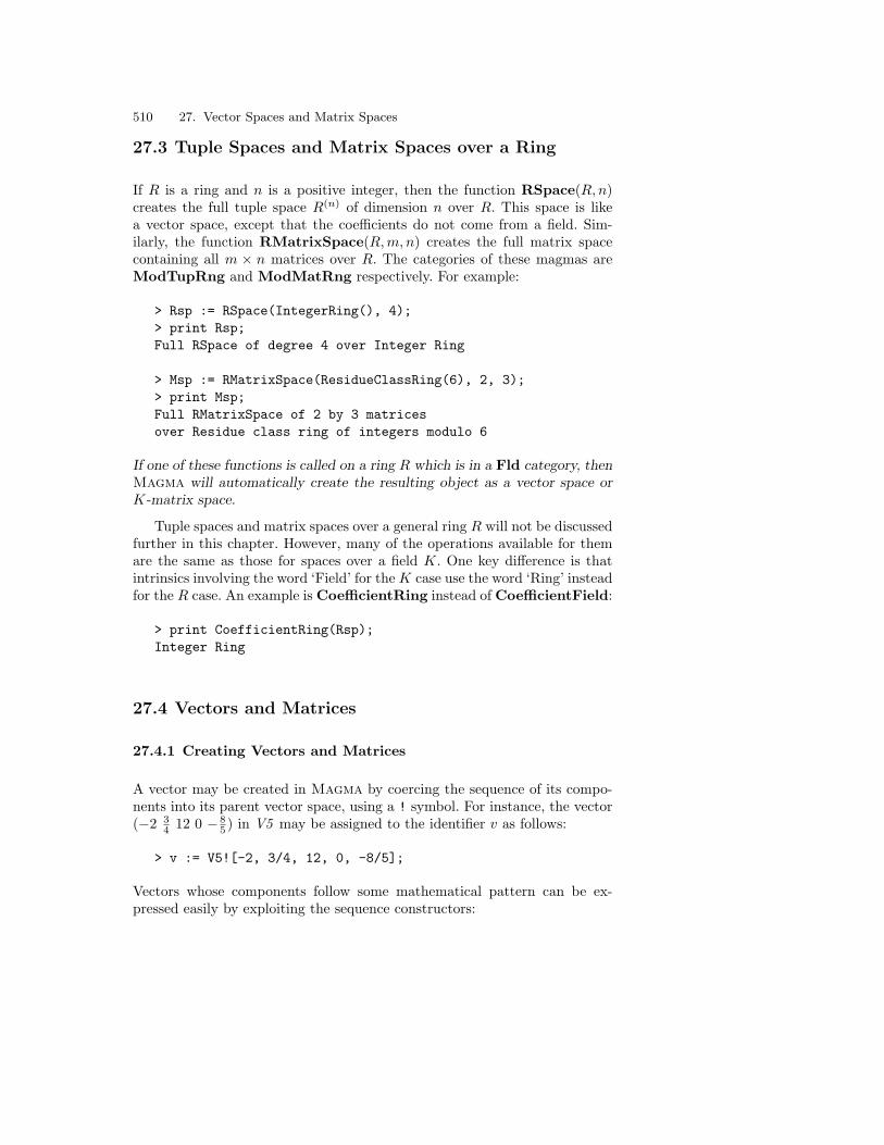
510 27. Vector Spaces and Matrix Spaces
27.3 Tuple Spaces and Matrix Spaces over a Ring
If R is a ring and n is a positive integer, then the function RSpace(R, n)creates the full tuple space R(n) of dimension n over R. This space is likea vector space, except that the coefficients do not come from a field. Sim-ilarly, the function RMatrixSpace(R,m, n) creates the full matrix spacecontaining all m × n matrices over R. The categories of these magmas areModTupRng and ModMatRng respectively. For example:
> Rsp := RSpace(IntegerRing(), 4);> print Rsp;Full RSpace of degree 4 over Integer Ring
> Msp := RMatrixSpace(ResidueClassRing(6), 2, 3);> print Msp;Full RMatrixSpace of 2 by 3 matricesover Residue class ring of integers modulo 6
If one of these functions is called on a ring R which is in a Fld category, thenMagma will automatically create the resulting object as a vector space orK-matrix space.
Tuple spaces and matrix spaces over a general ring R will not be discussedfurther in this chapter. However, many of the operations available for themare the same as those for spaces over a field K. One key difference is thatintrinsics involving the word ‘Field’ for the K case use the word ‘Ring’ insteadfor the R case. An example is CoefficientRing instead of CoefficientField:
> print CoefficientRing(Rsp);Integer Ring
27.4 Vectors and Matrices
27.4.1 Creating Vectors and Matrices
A vector may be created in Magma by coercing the sequence of its compo-nents into its parent vector space, using a ! symbol. For instance, the vector(−2 3
4 12 0 − 85 ) in V5 may be assigned to the identifier v as follows:
> v := V5![-2, 3/4, 12, 0, -8/5];
Vectors whose components follow some mathematical pattern can be ex-pressed easily by exploiting the sequence constructors:

27.4 Vectors and Matrices 511
> w := V5![3/4*(-1)^i: i in [1..5]];> print w;(-3/4 3/4 -3/4 3/4 -3/4)
The zero vector of a vector space V is V !0. The IsZero(v) function returnstrue when its argument is the zero vector.
Matrices are constructed in the same way, by regarding the matrix spaceas a vector space of dimension mn. The entries must be listed in row-majororder, the same order as for the standard basis. (This is the same method formatrix creation as is used in matrix rings and matrix groups.) For instance,the following lines construct two 3× 7 matrices with real coefficients:
> R20 := RealField(20);> M37 := KMatrixSpace(R20, 3, 7);> m1:=M37![0,0,0,4.5,1,1,-6.7,0,0,0,0,0,0,0,1,1,0,0,0,1,0];> print m1;[ 0 0 0 4.5 1 1 -6.7][ 0 0 0 0 0 0 0][ 1 1 0 0 0 1 0]> m2 := M37![ (21 - t) / 5 : t in [0..20] ];> print m2;[4.2 4 3.8 3.6 3.4 3.2 3][2.8 2.6 2.4 2.2 2 1.8 1.6][1.4 1.2 1 0.8 0.6 0.4 0.2]
Given a vector or matrix u, the function Eltseq(u) returns the sequenceof its components:
> print Eltseq(w);[ -3/4, 3/4, -3/4, 3/4, -3/4 ]> print Eltseq(m2);[ 4.2, 4, 3.8, 3.6, 3.4, 3.2, 3, 2.8, 2.6, 2.4, 2.2, 2, 1.8,1.6, 1.4, 1.2, 1, 0.8, 0.6, 0.4, 0.2 ]
If U is a vector space or matrix space defined over a finite field, thenRandom(U) returns a random element of U . (U has to be finite becauseotherwise Magma has no way of constructing random elements.) For exam-ple:
> for n in [1..4] dofor> print Random(V3F11);for> end for;( 9 10 2)( 5 4 2)

512 27. Vector Spaces and Matrix Spaces
( 8 0 6)( 6 8 6)
27.4.2 Arithmetic and Functions
The operators and functions in this subsection apply to both matrices andvectors. If the operations are performed on matrices, Magma considers thematrices to be vectors, by treating them in row-major order, but the outputfor matrices remains in rectangular form.
Arithmetic on Magma vectors and matrices is performed with the usualoperators. Addition and subtraction are performed component-by-component,so the vectors or matrices in the operation must be of the same size. Scalarmultiplication is also available. For instance, the vector y = v − 2
5w can beassigned as follows:
> y := v - 2/5*w; print y;(-17/10 9/20 123/10 -3/10 -13/10)
Normalization is a particular type of automatic scalar multiplication.Given a vector or matrix u, the function Normalize(u) returns u divided byits first non-zero component, so that the first non-zero entry of the result isthe unit of K5 . For instance:
> print Normalize(y);( 1 -9/34 -123/17 3/17 13/17)
The normalized form of a zero vector is the same as the vector itself.
Given u1 and u2 in the same space, InnerProduct(u, v) returns theirinner product according to whatever inner product is defined on the space(usually the Euclidean norm). For example, the following line calculates theinner product of vectors v and w in V 5 with respect to the Euclidean norm,so the output is the sum of the products of corresponding components of vand w:
> print InnerProduct(v, w);-459/80
27.4.3 Indexing Vectors and Matrices
The usual v[i] notation may be used to inspect or modify the ith componentof a vector v. For instance:

27.4 Vectors and Matrices 513
> print y[2];9/20> y[2] := 1000;> print y;(-17/10 1000 123/10 -3/10 -13/10)
The indexing of matrices is slightly different. To obtain an individualentry of a matrix, two coordinates are required. Given a matrix m, the entryin the ith row and jth column is m[i, j]:
> print m2[2, 6];1.8
By contrast, m[i] means the vector which is the ith row of m:
> print m2[3];[1.4 1.2 1 0.8 0.6 0.4 0.2]> print IsZero(m1[2]);true
There is no way of obtaining a column of m directly, since Magma’s vec-tors are row vectors. The best method is to transpose m, using the functionTranspose(m), and then extract a row from the transposed form. The nextexample shows how to obtain the fourth column of m as a row vector:
> m2tr := Transpose(m2);> print m2tr[4];(3.6 2.2 0.8)
The function Support(u) returns the set containing the indexes of all thenon-zero entries of a vector or matrix u. If u is a matrix, then the indexesare given as tuple pairs < i, j >:
> print Support(v); 1, 2, 3, 5 > print Support(m1); <1, 6>, <3, 1>, <1, 5>, <1, 4>, <3, 6>, <1, 7>, <3, 2>
27.4.4 Blocks within Matrices
Given an element A of a matrix space over K, any p × q block within itmay be considered as a matrix (in particular, an element of the space ofp× q matrices over K). Table 27.1 lists the operations connected with blockswithin matrices, and some examples are given below:

514 27. Vector Spaces and Matrix Spaces
Table 27.1. Blocks within matrices
Magma Meaning
Submatrix(A, i, j, p, q) p × q submatrix of A, starting at row i andcolumn j
InsertBlock(˜A, R, i, j) Given p × q matrix R, changes matrix A byreplacing the p× q submatrix starting at row iand column j with R
HorizontalJoin(A, B) Matrix formed by joining matrices A and Bhorizontally, where A and B have the samenumber of rows
HorizontalJoin(Q) Matrix formed by joining sequence Q of ma-trices horizontally, where the matrices all havethe same number of rows
VerticalJoin(A, B) Matrix formed by joining matrices A and Bvertically,
where A and B have the same number of columns
VerticalJoin(Q) Matrix formed by joining sequence Q of matri-ces vertically,
where the matrices all have the same number of columns
DiagonalJoin(A, B) Matrix formed by joining matrices A and Balong main diagonal, with zeros elsewhere
DiagonalJoin(Q) Matrix formed by joining sequence Q of matri-ces along main diagonal, with zeros elsewhere
> ms := Submatrix(m2, 2, 3, 2, 4); print ms;[2.4 2.2 2 1.8][ 1 0.8 0.6 0.4]> InsertBlock(~m1, ms, 2, 1);> print m1;[ 0 0 0 4.5 1 1 -6.7][ 2.4 2.2 2 1.8 0 0 0][ 1 0.8 0.6 0.4 0 1 0]> print VerticalJoin(m1, m2);[ 0 0 0 4.5 1 1 -6.7][ 2.4 2.2 2 1.8 0 0 0][ 1 0.8 0.6 0.4 0 1 0][ 4.2 4 3.8 3.6 3.4 3.2 3][ 2.8 2.6 2.4 2.2 2 1.8 1.6][ 1.4 1.2 1 0.8 0.6 0.4 0.2]> print DiagonalJoin(ms, m2);[2.4 2.2 2 1.8 0 0 0 0 0 0 0][ 1 0.8 0.6 0.4 0 0 0 0 0 0 0][ 0 0 0 0 4.2 4 3.8 3.6 3.4 3.2 3][ 0 0 0 0 2.8 2.6 2.4 2.2 2 1.8 1.6]

27.5 Subspaces and Quotient Spaces 515
[ 0 0 0 0 1.4 1.2 1 0.8 0.6 0.4 0.2]
27.5 Subspaces and Quotient Spaces
Vector subspaces and quotient spaces may be formed in Magma using thecustomary sub and quo constructors. For instance, the following statementassigns to V5s the subspace of V5 generated by w, the third generator of V5and the vector (−5 5 7 5 −5):
> V5s := sub< V5 | w, V5.3, [-5, 5, 7, 5, -5] >;
The information listed to the right of the | symbol specifies the generatorsfor the subspace. In this example they are given explicitly as vectors. Otherpossible objects on the right of the | symbol are subspaces of the mainspace, and sets or sequences containing these; in this case, the vectors usedto generate the subspace will be the generating elements of these subspaces.
Not all vector spaces are represented internally using the generators pro-vided by the user. For the sake of efficiency, Magma employs an echelonizedbasis for this purpose, and the vectors of this basis may differ from thosevectors given by the user. However, the generators are all stored (even if theyare not linearly independent), and are available in the user-specified orderunder the names V5s.1, V5s.2 and V5s.3. For example:
> print V5s;Vector space of degree 5, dimension 2 over Rational FieldGenerators:(-3/4 3/4 -3/4 3/4 -3/4)( 0 0 1 0 0)( -5 5 7 5 -5)Echelonized basis:( 1 -1 0 -1 1)( 0 0 1 0 0)> print 10*V5s.2 + V5s.3;(-5 5 17 5 -5)
The quotient constructor quo creates the quotient of the main space bythe subspace described by whatever is on the right of the | symbol. Forinstance, the following lines demonstrate two ways to create the quotientV5q of V5 by V5s:
> V5q := quo< V5 | V5s >;> // or

516 27. Vector Spaces and Matrix Spaces
> V5q := quo< V5 | w, V5.3, [-5, 5, 7, 5, -5] >;> print V5q;Full Vector space of degree 3 over Rational Field
The sub and quo constructors can return mappings as their second re-turn value. These mappings are the inclusion homomorphism and the naturalhomomorphism, respectively. For instance, we can construct the natural ho-momorphism phi which maps V5 to the quotient space V5q . In accordancewith vector space theory, the complement C of V5s is isomorphic to V5q ,since C and V5q have the same dimension:
> V5q, phi := quo< V5 | w, V5.3, [-5, 5, 7, 5, -5] >;> print phi;Mapping from: Full Vector space of degree 5 over RationalField to Full Vector space of degree 3 over Rational Field> C := Complement(V5, V5s); print C;Vector space of degree 5, dimension 3 over Rational FieldEchelonized basis:(0 1 0 0 0)(0 0 0 1 0)(0 0 0 0 1)> print C@phi;Full Vector space of degree 3 over Rational Field> print C@phi eq V5q;true
The following line verifies that the kernel of phi is V5s:
> print Kernel(phi) eq V5s;true
If the user has constructed a subspace or quotient space U of a vectorspace V , without obtaining the corresponding mapping, the mapping can beobtained at some later stage from the function Morphism(U, V ). It returnsthe homomorphism as a matrix.
27.6 Operations on Vector Spaces
Table 27.2 lists several of the Magma operations on vector spaces. Notecarefully the difference between generators and basis vectors.

27.7 Operations with Linear Transformations 517
Table 27.2. Vector space operations
Magma Meaning
CoefficientField(V ),BaseField(V ) Field K of K-vector space V
Dimension(V ) Dimension of V
Generic(V ) Full vector space K(n) of which V isa subspace
OverDimension(V ), Degree(V ) Given subspace V of K(n), returnsn
OverDimension(v), Degree(V ) Given element v of subspace of K(n),returns n
Generators(V ) Set of the generators of V , as givento Magma (e.g., in sub)
Ngens(V ) Number of generators of V
V .i ith generator of V
Basis(V ) Sequence of basis vectors of V , ascalculated by Magma
BasisMatrix(V ) Matrix whose rows are the basis vec-tors of V
BasisElement(V, i) ith basis vector of V
U1 + U2 Sum of subspaces U1 and U2
U1 meet U2 Intersection of subspaces U1 and U2
Complement(V, U) Complement for subspace U of V , asa subspace of V
Transversal(V, U) Transversal in V for subspace U ofV , as a set of vectors; V must beover a finite field
27.7 Operations with Linear Transformations
Given any two K-vector spaces V and W of over-dimension (degree) m and n,the set of linear transformations from V to W is the homomorphism moduleHom(V,W ). Every linear transformation V → W can be written as a matrixa of size m× n with entries in K. The effect of a on V may be investigatedusing mapping operations.
For example, let the field K be the quadratic field Q(√
7), and let V andW be certain subspaces of the vector spaces K(4) and K(6):
> K<rt7> := QuadraticField(7); print K;Quadratic Field Q(rt7)> V := sub< VectorSpace(K, 4) |> [rt7, 1, 0, 0], [0, 3 - 2*rt7, 0, 1] >;> print V;Vector space of degree 4, dimension 2

518 27. Vector Spaces and Matrix Spaces
over Quadratic Field Q(rt7)Generators:( rt7 1 0 0)( 0 3 - 2*rt7 0 1)Echelonized basis:(1 0 0 1/133*(14 + 3*rt7))(0 1 0 1/19*(-3 - 2*rt7))> W := sub< VectorSpace(K, 6) |> [2,0,0,1,0,0], [0,0,0,0,-1,1], [0,1,0,0,0,0] >;> print W;Vector space of degree 6, dimension 3over Quadratic Field Q(rt7)Generators:( 2 0 0 1 0 0)( 0 0 0 0 -1 1)( 0 1 0 0 0 0)Echelonized basis:( 1 0 0 1/2 0 0)( 0 1 0 0 0 0)( 0 0 0 0 1 -1)>> H := Hom(V, W);> print H;KMatrixSpace of 4 by 6 GHom matrices and dimension 18 overQuadratic Field Q(rt7)
Let a equal the sum of the second generator of H and twice the thirteenthgenerator of H. It has domain V and codomain W : be the us construct thefollowing matrix a:
> a := H.2 + 2*H.13;> print a;[0 1 0 0 0 0][0 0 0 0 0 0][0 0 0 2 0 0][0 0 0 0 0 0]> print Domain(a) eq V and Codomain(a) eq W;true
The product of an element of V and a is an element of W . For instance:
> v := V![ -8*rt7, -2 - 4*rt7, 0, 2];> w := v * a; print w;( 0 -8*rt7 0 0 0 0)> print Coordinates(W, w);
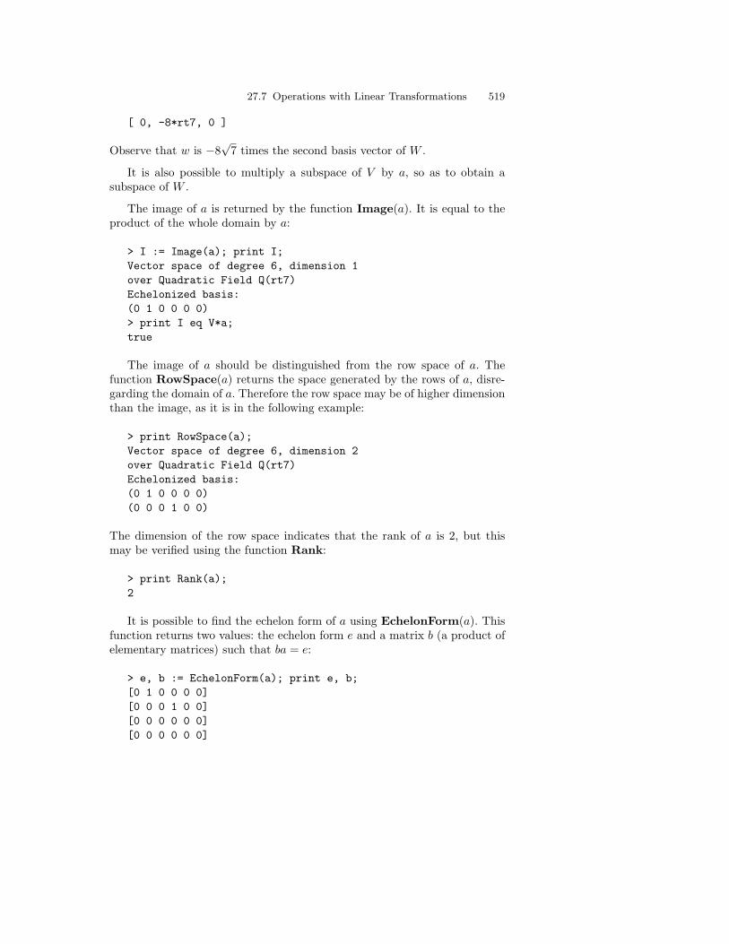
27.7 Operations with Linear Transformations 519
[ 0, -8*rt7, 0 ]
Observe that w is −8√
7 times the second basis vector of W .
It is also possible to multiply a subspace of V by a, so as to obtain asubspace of W .
The image of a is returned by the function Image(a). It is equal to theproduct of the whole domain by a:
> I := Image(a); print I;Vector space of degree 6, dimension 1over Quadratic Field Q(rt7)Echelonized basis:(0 1 0 0 0 0)> print I eq V*a;true
The image of a should be distinguished from the row space of a. Thefunction RowSpace(a) returns the space generated by the rows of a, disre-garding the domain of a. Therefore the row space may be of higher dimensionthan the image, as it is in the following example:
> print RowSpace(a);Vector space of degree 6, dimension 2over Quadratic Field Q(rt7)Echelonized basis:(0 1 0 0 0 0)(0 0 0 1 0 0)
The dimension of the row space indicates that the rank of a is 2, but thismay be verified using the function Rank:
> print Rank(a);2
It is possible to find the echelon form of a using EchelonForm(a). Thisfunction returns two values: the echelon form e and a matrix b (a product ofelementary matrices) such that ba = e:
> e, b := EchelonForm(a); print e, b;[0 1 0 0 0 0][0 0 0 1 0 0][0 0 0 0 0 0][0 0 0 0 0 0]
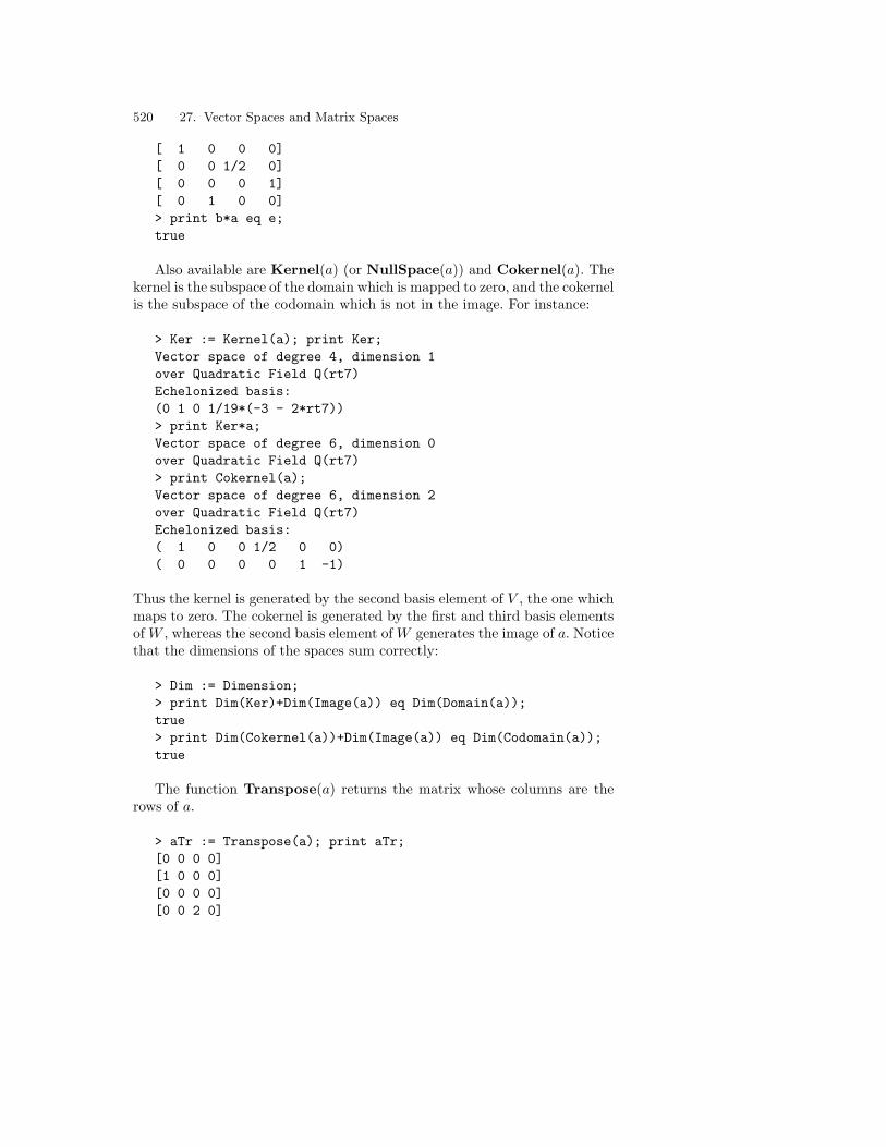
520 27. Vector Spaces and Matrix Spaces
[ 1 0 0 0][ 0 0 1/2 0][ 0 0 0 1][ 0 1 0 0]> print b*a eq e;true
Also available are Kernel(a) (or NullSpace(a)) and Cokernel(a). Thekernel is the subspace of the domain which is mapped to zero, and the cokernelis the subspace of the codomain which is not in the image. For instance:
> Ker := Kernel(a); print Ker;Vector space of degree 4, dimension 1over Quadratic Field Q(rt7)Echelonized basis:(0 1 0 1/19*(-3 - 2*rt7))> print Ker*a;Vector space of degree 6, dimension 0over Quadratic Field Q(rt7)> print Cokernel(a);Vector space of degree 6, dimension 2over Quadratic Field Q(rt7)Echelonized basis:( 1 0 0 1/2 0 0)( 0 0 0 0 1 -1)
Thus the kernel is generated by the second basis element of V , the one whichmaps to zero. The cokernel is generated by the first and third basis elementsof W , whereas the second basis element of W generates the image of a. Noticethat the dimensions of the spaces sum correctly:
> Dim := Dimension;> print Dim(Ker)+Dim(Image(a)) eq Dim(Domain(a));true> print Dim(Cokernel(a))+Dim(Image(a)) eq Dim(Codomain(a));true
The function Transpose(a) returns the matrix whose columns are therows of a.
> aTr := Transpose(a); print aTr;[0 0 0 0][1 0 0 0][0 0 0 0][0 0 2 0]

27.8 Row and Column Operations 521
[0 0 0 0][0 0 0 0]
Multiplying matrices from different homomorphism modules is anotherway of creating elements of new homomorphism modules. The process cor-responds to the composition of mappings. If U is a subspace of some otherK-vector space and b is an element of Hom(W,U), then the matrix producta*b represents the mapping in Hom(V, U) which is the composition of a andb.
27.8 Row and Column Operations
Table 27.3. Row and column operations
Magma Meaning
AddRow(˜a, u, i, j) Adds u times row i to row j in matrix a
AddColumn(˜a, u, i, j) Adds u times column i to row j in matrix a
MultiplyRow(˜a, u, i) Multiplies row i of matrix a by u
MultiplyColumn(˜a, u, i) Multiplies column i of matrix a by u
SwapRows(˜a, i, j) Interchanges rows i and j of matrix a
SwapColumns(˜a, i, j) Interchanges columns i and j of matrix a
The three elementary row and column operations on matrices are availableas procedures in Magma. Table 27.3 shows them. Each procedure destruc-tively modifies the given matrix, so a ˜ must precede its identifier name inthe procedure call. In the following example, a copy a1 of a is made, and then17 times row 1 of a1 is added to row 4, and columns 2 and 5 are swapped:
> a1 := a; print a1;[0 1 0 0 0 0][0 0 0 0 0 0][0 0 0 2 0 0][0 0 0 0 0 0]> AddRow(~a1, 17, 1, 4); print a1;[ 0 1 0 0 0 0][ 0 0 0 0 0 0][ 0 0 0 2 0 0][ 0 17 0 0 0 0]> SwapColumns(~a1, 2, 5); print a1;[ 0 0 0 0 1 0]

522 27. Vector Spaces and Matrix Spaces
[ 0 0 0 0 0 0][ 0 0 0 2 0 0][ 0 0 0 0 17 0]
27.9 Simultaneous Systems of Linear Equations
Magma provides an easy way of solving a simultaneous system of linearequations that is expressed as a matrix equation V X = W , where X is amatrix, W is a vector with the same number of entries as X has columns, andV is an unknown vector with the same number of entries as X has rows. Thefunction Solution(X, W ) returns a particular solution v, and also returnsthe kernel K of X, regarding X as a homomorphism from the vector spaceof V to the vector space of W . The kernel is the space of vectors which whenmultiplied by X equal the zero vector, so the general solution to V X = W isV = v + k where k is any vector in K. For example, suppose the user wantsto solve the system
a + 2b + 2c − 3d = 52a − b + c + 2d = 13a + b + 3c − d = 6
which is equivalent, once the vectors are written as row vectors, to
(a b c d
)
1 2 32 −1 12 1 3
−3 2 −1
=
(5 1 6
)
In Magma this system may be solved as follows:
To perform this example online, type load "I96c27e1";
> Q := RationalField();> V4 := VectorSpace(Q, 4);> V3 := VectorSpace(Q, 3);> H43 := Hom(V4, V3);> X := H43![1, 2, 3, 2, -1, 1, 2, 1, 3, -3, 2, -1];> print X;[ 1 2 3][ 2 -1 1][ 2 1 3]

27.10 Changing the Basis 523
[-3 2 -1]> W := V3![5, 1, 6];> v, K := Solution(X, W);> print v;(7/5 9/5 0 0)> print K;Vector space of degree 4, dimension 2 over Rational FieldEchelonized basis:( 1 0 -8/7 -3/7)( 0 1 -1/7 4/7)
The identifier v now contains a particular solution to the equation, and Kcontains the kernel of X:
> print v*X eq W and Kernel(X) eq K;true
Therefore the general solution is V = ( 75
95 0 0)+t1(1 0 −8
7−37 )+t2(0 1 −1
747 ).
If the user is not sure whether there is a solution to the equation V X =W , then IsConsistent(X, W ) should be used instead. It returns true if asolution exists, and if so, then it also returns a particular solution and thekernel, just as Solution does:
> print IsConsistent(X, V3![5, 1, 7]);false> print IsConsistent(X, W);true (7/5 9/5 0 0)
Vector space of degree 4, dimension 2 over Rational FieldEchelonized basis:( 1 0 -8/7 -3/7)( 0 1 -1/7 4/7)
27.10 Changing the Basis
27.10.1 Defining the Chosen Basis
The function VectorSpaceWithBasis(B), where B is a sequence of linearlyindependent vectors, allows the user to define a chosen basis B for a vectorspace. (An alternative version of this function takes as its argument not asequence but a matrix whose rows are the basis vectors.) For example, thefollowing lines show how to build a vector space Sw of degree 3 over the

524 27. Vector Spaces and Matrix Spaces
rationals which has the basis [[1, 0, 1], [2, 1, 1], [1, 1, 1]], as compared to thesame vector space S with the standard basis:
To perform this example online, type load "I96c27e2";
> S := VectorSpace(RationalField(), 3);> print Basis(S);[
(1 0 0),(0 1 0),(0 0 1)
]> Sw:=VectorSpaceWithBasis([S | [1,0,1], [2,1,1], [1,1,1]]);> print Basis(Sw);[
(1 0 1)(2 1 1)(1 1 1)
]
The vector spaces S and Sw are considered by Magma to be the same inmost respects. Note especially that when a vector is being created it makesno difference whether the sequence of its entries is coerced into S or Sw :
> print S eq Sw;true> print S![2, 5, 72] eq Sw![2, 5, 72];true
The only time that the basis of Sw is significant, apart from when us-ing the functions that access the basis and generators, is for the functionCoordinates(V, v). Given a vector v in a vector space V , it returns thecoordinates of v relative to the current basis of V . For example:
> v := Sw![-2, -1, 2];> print v;(-2 -1 2)> print Coordinates(Sw, v);[ 3, -4, 3 ]
Observe that v = 3 · (1 0 1)− 4 · (2 1 1) + 3 · (1 1 1).
To simulate a vector space whose entries are radically connected with anon-standard basis, the user should create a matrix which maps the vectorsof the standard basis to those of the required basis:

27.10 Changing the Basis 525
> M := EndomorphismAlgebra(S); print M;Full Matrix Algebra of degree 3 over Rational Field> m := M![1,0,1, 2,1,1, 1,1,1];> /* the rows are the non-standard basis vectors */> mInv := m^-1; print mInv;[ 0 1 -1][-1 0 1][ 1 -1 1]
Now, given a vector, it may be multiplied on the right by mInv to make itinto as a vector expressed relative to the other basis:
> print S![-2, -1, 2]*mInv;( 3 -4 3)
The output is a vector of the simulated vector space.
27.10.2 Constructing a Basis Gradually
Magma provides some functions to help the user construct linearly inde-pendent vectors. The simplest of these is IsIndependent(S), which returnstrue if the elements of the set or sequence S are linearly independent. Forexample:
> vecseq := [V5 | [4/3, 8, -2, 0, 1/2], [5, 7, 10, -2, 0]];> print IsIndependent(vecseq);true
The function ExtendBasis(Q,V ) constructs a basis for a vector space Vsuch that the linearly independent sequence of vectors Q is the first part ofthe resulting basis sequence:
> print ExtendBasis(vecseq, V5);[
(4/3 8 -2 0 1/2),( 5 7 10 -2 0),(0 0 1 0 0),(0 0 0 1 0),(0 0 0 0 1)
]
The space V need not be a full vector space.

526 27. Vector Spaces and Matrix Spaces
Another form of this function is ExtendBasis(U, V ), which takes a sub-space U of V as its first argument. The basis sequence that it constructsbegins with the basis of U .
27.11 Changing the Coefficient Field
The functions ExtendField(V, L) and RestrictField(V,L) change the fieldK of a vector space V to the field L, where K and L are both finite fields.Both functions return two values, namely the L-vector space U and a homo-morphism V → U .
For ExtendField(V,L), L must be an extension of K. The vector spacereturned is V ⊗KL and the mapping returned is the inclusion homomorphism.
For RestrictField(V, L), L must be a subfield of K, where the generatingvectors for K lie over L. U is obtained from V by restricting the scalars toL, and the mapping returned is the restriction homomorphism.
A more general function for this task is ChangeRing(V, R). It returnsthe vector space V ′ over R obtained by coercing the components of elementsof V into V ′, together with the homomorphism from V to V ′. If the userwishes to use a special homomorphism f from the old coefficient ring to R,then use the function should be used in the form ChangeRing(V, R, f).

28. Matrix Algebras
This chapter discusses matrix algebras (matrix rings) in Magma. In general,it does not list the operations that also apply to other categories of rings. SeeChapter 19 for these.
28.1 The Generic Matrix Algebra and Its Elements
28.1.1 Constructing the Generic Matrix Algebra
The set of all n × n matrices with entries in a ring R forms an R-algebraMn(R) which can be constructed in Magma as MatrixAlgebra(R, n). SinceMn(R) may also be regarded as a (non-commutative) ring, another name forthis function is MatrixRing(R, n). The category of M is AlgMat.
For example, the algebra M below is the generic or complete matrix al-gebra of degree 3 over F , the finite field of five elements:
> F := FiniteField(5);> M := MatrixAlgebra(F, 3);> print M;Full Matrix Algebra of degree 3 over GF(5)> print #M;1953125
This algebra has 532= 1953125 elements.
28.1.2 Constructing Matrices
The method for defining an element of a matrix algebra is to create a sequenceof its entries, listed in row-major order, and coerce it into the algebra. (Thisis the same method for matrix creation as is used in matrix spaces and matrixgroups.) Continuing the example:

528 28. Matrix Algebras
> m1 := M![2, 3, 0, 1, 1, 0, 0, 3, 4]; print m1;[2 3 0][1 1 0][0 3 4]
Notice that for this coefficient ring, Magma is able to coerce the integerelements of the sequence into elements of F , so that the universe of the givensequence need not be F .
Matrices which have the same entry t down the main diagonal and zeroseverywhere else are called scalar matrices, because they behave very muchlike the element t in the coefficient ring R. For this reason, such matrices maybe created by coercing t into the matrix algebra:
> m2 := M!4; print m2;[4 0 0][0 4 0][0 0 4]
An alternative for M !t is ScalarMatrix(M, t).
Being a scalar matrix, the zero matrix may be constructed as M !0.Zero(M) also returns this matrix.
Another special kind of matrix is a diagonal matrix. Its entries are all zerosexcept for those down the main diagonal (from top left to bottom right). Thefunction for creating a diagonal matrix is DiagonalMatrix(M, Q). Given amatrix algebra M over R of degree n, and a sequence Q of n elements of R,it returns the matrix in M with elements of Q down the main diagonal andzeros elsewhere. For instance:
> print DiagonalMatrix(M, [4, 2, 3]);[4 0 0][0 2 0][0 0 3]
Magma also has a function MatrixUnit(M, i, j) for constructing a ma-trix unit, that is, a matrix in M which has the one of the coefficient ring inrow i, column j and zeros everywhere else:
> print MatrixUnit(M, 3, 2);[0 0 0][0 0 0][0 1 0]

28.1 The Generic Matrix Algebra and Its Elements 529
Scalar matrices, diagonal matrices and matrix units may all be con-structed by coercing a sequence of length n2 into the matrix algebra, butthe functions above make the task easier in these frequently-occurring cases.
The function ElementToSequence(m) or Eltseq(m) converts a matrixm into the sequence of its entries, in row-major order:
> print Eltseq(m1);[ 2, 3, 0, 1, 1, 0, 0, 3, 4 ]
28.1.3 Arithmetic on Matrices
Arithmetic on elements of matrix algebras is performed with the usual ringoperators for addition and multiplication. (Remember, however, that matrixmultiplication is not commutative in general.) For example:
> print m1 * m2;[3 2 0][4 4 0][0 2 1]> print m1^-1;[4 3 0][1 3 0][3 4 4]
Observe that the inverse of an invertible matrix is calculated by raising it tothe power of −1. The function IsUnit(m) is provided for testing whether amatrix m has an inverse.
It was shown above that scalar matrices may be constructed by coercingthe scalar into the algebra. This is an instance of forced coercion. However,automatic coercion of scalars into matrix algebras may also occur. When ascalar matrix is involved in an arithmetic operation with another matrix,the scalar matrix may be referred to by means of the scalar alone, withoutexplicitly coercing the scalar into the matrix algebra:
> print m1 - 2;[0 3 0][1 4 0][0 3 2]
It is possible to access and modify specific entries or rows of a matrix.The entry in row i, column j of matrix m is m[i, j], and the ith row is m[i].For instance:

530 28. Matrix Algebras
> r := m1[3]; print r;(0 3 4)> m2[3,2] := 2; print m2;[4 0 0][0 4 0][0 2 4]> m2[1] := r; print m2;[0 3 4][0 4 0][0 2 4]
Multiplication involving matrices is possible not only when the two ma-trices are elements of (or coercible into) the same matrix algebra, but alsowhenever the coefficient rings are compatible and the number of columns ofthe first matrix equals the number of rows of the second matrix. For examplesof this, using rectangular matrices belonging to matrix spaces, see Chapter27. The operations on blocks within matrices listed in Table 27.1 are alsoavailable.
28.2 Constructing Other Matrix Algebras
28.2.1 Subalgebras
The matrix algebra discussed to this point has been the generic or full matrixalgebra Mn(R), which is constructed using the function MatrixAlgebra(R, n).There are two main ways to create subalgebras of this. One method is tobuild Mn(R) first, then use a sub constructor. The other method is to usethe MatrixAlgebra or MatrixAlgebra constructor
MatrixAlgebra< R,n | generator specification >
which builds the subalgebra of the generic algebra in one step. In both ver-sions, the generators of the algebra must be given on the right side of the |symbol in the constructor. The result is the same in either case:
> Ms := MatrixAlgebra< F, 3 |> [2,3,0, 1,1,0, 0,3,4] >;> print Ms;Matrix Algebra of degree 3 with 1 generator over GF(5)> print #Ms;125> print Ms eq sub< M | m1 >;true

28.2 Constructing Other Matrix Algebras 531
Now Ms is a matrix algebra with one generator, m1 .
Unlike M , the subalgebra Ms does not contain all the 3× 3 matrices overF , so it is not a generic algebra. The function Generic(S) returns the genericalgebra corresponding to a matrix algebra S:
> print Generic(Ms) eq M;true
Matrix algebras do not have to contain the multiplicative identity of theirgeneric algebra. The generators are exactly those given by the user; the oneof the generic algebra is not inserted automatically among the generators.For example:
> print M!1 in> sub< M | [0,0,0,0,2,0,0,2,0], [0,0,0,0,0,2,0,0,0] >;false
28.2.2 Ideals
Since matrix algebras are generally non-commutative, there are three kindsof ideals: left ideal, right ideal and two-sided ideal. The constructors for theseare respectively lideal, rideal and ideal. See Section ??. A left ideal of amatrix algebra M is a subalgebra I of M with the property that for all i ∈ Iand m ∈ M , the product mi is in I. A right ideal satisfies the property im ∈ I,and a two-sided ideal (or simply ‘ideal’) satisfies both these properties. Forexample:
> LI := lideal< M | M.1 >;> print LI;Matrix Algebra [lideal of M] of degree 3 and dimension 3over GF(5)> m := Random(M);> print forall i: i in LI | m*i in LI ;true> print forall i: i in LI | i*m in LI ;false
The generic matrix algebra over a field has only two ideals, itself and thetrivial algebra, so examples of two-sided ideals must come from non-genericalgebras. Consider the set T consisting of all the 5 × 5 matrices with zerosbelow the diagonal over the finite field with 7 elements. This set, which formsa ring, is conveniently generated by all the matrix units in which the one isabove or the diagonal. The subset B of T consisting of the matrices that also

532 28. Matrix Algebras
have zeros on the diagonal may be shown to be an ideal of T . B is generatedby those matrix units which are above the diagonal. In Magma, T and Bmay be constructed as follows:
> T := MatrixAlgebra< GF(7), 5 |> MatrixUnit($, i, j) : i in [1..j], j in [1..5] >;> print T;Matrix Algebra of degree 5 with 15 generators over GF(7)> B := ideal< T |> MatrixUnit($, i, j) : i in [1..j-1], j in [1..5] >;> print B;Matrix Algebra [ideal of T] of degree 5 and dimension 10over GF(7)
Table 28.1. Operations involving ideals
Magma Meaning
JacobsonRadical(M) Intersection of all maximal ideals of algebra M
MaximalIdeals(M) Maximal (two-sided) ideals of M
MaximalLeftIdeals(M) Maximal left ideals of M
MaximalRightIdeals(M) Maximal right ideals of M
MinimalIdeals(M) Minimal (two-sided) ideals of M
MinimalLeftIdeals(M) Minimal left ideals of R
MinimalRightIdeals(M) Minimal right ideals of R
IsSimple(M) true if M has no non-trivial ideals
IsSemisimple(M) true if M is a direct sum of simple ideals (i.e.,has trivial Jacobson radical)
Table 28.1 (p. 532) lists functions relating to ideals of matrix algebras.The functions returning the maximal and minimal ideals (two-sided, left,and right) return them as a sequence of ideals, in non-decreasing size. Eachof these functions has a parameter Limit (default ∞): if the user assigns nto Limit, then at most n ideals will be calculated. The second return valueof the function will be true if all the ideals have been returned, else false.For instance:
> print MinimalIdeals(Ms);[
Matrix Algebra [ideal of Ms] of degree 3and dimension 1 over GF(5),
Matrix Algebra [ideal of Ms] of degree 3and dimension 2 over GF(5)

28.2 Constructing Other Matrix Algebras 533
]true
> T := MatrixAlgebra< GF(7), 5 |> MatrixUnit($, i, j) : i in [1..j], j in [1..5] >;> print MaximalIdeals(T);[
Matrix Algebra [ideal of T] of degree 5and dimension 14 over GF(7),
Matrix Algebra [ideal of T] of degree 5and dimension 14 over GF(7),
Matrix Algebra [ideal of T] of degree 5and dimension 14 over GF(7),
Matrix Algebra [ideal of T] of degree 5and dimension 14 over GF(7),
Matrix Algebra [ideal of T] of degree 5and dimension 14 over GF(7)]true> print MaximalIdeals(T : Limit := 2);[
Matrix Algebra [ideal of T] of degree 5and dimension 14 over GF(7),
Matrix Algebra [ideal of T] of degree 5and dimension 14 over GF(7)]false
28.2.3 Quotients
The quotient of a matrix algebra by an ideal is performed in Magma usingthe quo constructor. It returns an algebra, and a homomorphism from theoriginal algebra to the quotient. Continuing the example above:
> Q, f := quo< T | B >;> print Q;Algebra of dimension 5 with base ring GF(7)> print f;Mapping from: AlgMat: T to AlgCon: Q
The kernel of this homomorphism f is the ideal B used to construct thequotient:
> print Kernel(f) eq B;

534 28. Matrix Algebras
true
Q is isomorphic to the image f(D) of the subalgebra D of T consisting ofall the diagonal matrices. The reason is that T may be seen as the disjointunion of the cosets B + d, where d ∈ D. This may be seen by calculatingthe matrix that gives the correspondence between them, using the functionMorphism. The matrix returned by Morphism is square and has full rank,indicating an isomorphism:
> D := sub< T | MatrixUnit($, i, i) : i in [1..5] >;> print D;Matrix Algebra of degree 5 with 5 generators over GF(7)> print f(D);Algebra of dimension 5 with base ring GF(7)> print Morphism(Q, f(D));[1 0 0 0 0][0 0 0 0 1][0 0 0 1 0][0 0 1 0 0][0 1 0 0 0]
28.2.4 Other Matrix Algebra Constructions
Table 28.2. Other matrix algebra constructions
Magma Meaning
DirectSum(M, N) Direct sum of algebras M and N over same basering, with action given by direct sum of their actions
TensorProduct(M, N) Tensor product of M and N over same base ring
DirectSum(a, b) Direct sum of matrices a and b, as an element of thedirect sum of their parents
TensorProduct(a, b) Tensor product of a (n1 rows) and b (n2 rows) as anelement of Mn1n2(R)
ExteriorSquare(a) Given a ∈ Mn(R), return exterior square of a as anelement of Mn(n+1)(R)
SymmetricSquare(a) Given a ∈ Mn(R), return symmetric square of a asan element of Mn(n−1)(R)
Table 28.2 lists some constructions that are special to matrix algebras.For example:
> matrand := Random(Ms); print DirectSum(matrand, matrand);

28.3 General Facts About a Matrix Algebra 535
[2 1 0 0 0 0][2 0 0 0 0 0][1 3 2 0 0 0][0 0 0 2 1 0][0 0 0 2 0 0][0 0 0 1 3 2]
28.3 General Facts About a Matrix Algebra
Table 28.3. General facts about a matrix algebra
Magma Meaning
Degree(M) Degree n of M , an algebra of n× n matrices
Dimension(M) Dimension of M (base ring must be a field)
CoefficientRing(M),BaseRing(M)
Coefficient ring or base ring R of M
Generic(M) Given M of degree n and coefficient ring R, returnfull matrix algebra Mn(R) in which M is naturallyembedded
Table 28.3 summarizes the functions giving facts about a matrix algebra,and Table 28.4 gives the functions for individual matrices.
For example, if A is a square matrix over C, then A is Hermitian if itequals the sum of its complex conjugate and its transpose, and it is anti-Hermitian if the negative of A equals this sum. It can be shown that everysquare matrix over C may be written as the sum of a Hermitian matrix and ananti-Hermitian matrix. The following functions (ignoring issues of precision)may be used to represent a matrix in this way:
> HermitianPart := function(A)> H := Transpose(A);> n := Nrows(A);> for i in [1..n] do> for j in [1..n] do> H[i,j] := ComplexConjugate(H[i,j]);> end for;> end for;> return H;> end function;> // OR

536 28. Matrix Algebras
Table 28.4. General facts about elements of matrix algebras
Magma Meaning
NumberOfRows(a),Nrows(a) Number of rows of a
NumberOfColumns(a),Ncolumns(a) Number of columns of a
Rank(a) Rank of a
Determinant(a) Determinant of a
Trace(a) Sum of diagonal entries of a
Transpose(a) Transpose of a
Order(a) Given invertible matrix a over afinite field, return the order of a
FactoredOrder(a) Given invertible matrix a over afinite field, return the order of a,in a factorization sequence
IsDiagonal(a) true if the only non-zero entries ofa are on the diagonal
IsScalar(a) true if a is a diagonal matrix, andall the entries on the diagonal arethe same
IsSymmetric(a) true if a equals its transpose
IsSimilar(a, b) true if a and b are similar; if true,also returns matrix t such thattat−1 = b
> HermitianPart := func< A |> Parent(A) ! [ ComplexConjugate(A[j,i]) :> i, j in [1..Nrows(A)] ] >;
> HermAnti := func< A | B, A - B> where B is 1/2*(A + HermitianPart(A)) >;
> C<i> := ComplexField();> M4C := MatrixAlgebra(C, 4);> s1 := [ Random(20): n in [1..16] ];> s2 := [ Random(20): n in [1..16] ];> A := M4C!s1 + i*M4C!s2;> print A;[18 + 11*i 16 + 12*i 20 11 + 4*i][ 9*i 11 + 16*i 2 + 20*i 18 + 19*i][ 18 20 + 3*i 20 + 10*i 6 + 13*i][ 1 + 7*i 5 + 15*i 19 + 1*i 7 + 5*i]> B, C := HermAnti(A);> print A eq B+C;true> print B eq HermitianPart(B);

28.4 Linear Algebra Concepts 537
true> print -C eq HermitianPart(C);true
28.4 Linear Algebra Concepts
It has already been seen that it is possible to multiply a square matrix bya scalar, or to multiply two square or rectangular matrices of suitable sizes.Another kind of multiplication for matrix algebras is the product v*m ofa (row) vector v with a matrix m. Here v and m must have compatiblecoefficient rings, and v must have the same number of columns as m has rows.For instance, the vector r constructed on p. 529 is suitable for multiplicationwith a matrix of M :
> print r * m1;(3 0 1)
The value returned belongs to the generic vector space V over the coefficientring of M and with the same degree as M :
> V := Parent(r); print V;Full Vector space of degree 3 over GF(5)> print V eq VectorSpace(F, 3);true
V is the natural structure on which M acts, and may also be obtainedusing the function BaseModule(M):
> print V eq BaseModule(M);true
For any matrix algebra M of degree n over a ring R, BaseModule(M)returns the generic R-module of rank n, consisting of n-tuples over R. WhenR is a field, the R-module will be a vector space over R.
Given any m in a matrix algebra, the function given by v 7→ vm for v ∈ Vis an endomorphism of V , where V is the base module of the parent of m.The functions Kernel(m) and Image(m) return the standard submodulesof V relating to this endomorphism. For example:
> print Kernel(m2);Vector space of degree 3, dimension 1 over GF(5)Echelonized basis:

538 28. Matrix Algebras
(1 1 4)> print Image(m2);Vector space of degree 3, dimension 2 over GF(5)Echelonized basis:(0 1 0)(0 0 1)
The kernel contains the elements of V which map to zero, and the imagecontains all the elements to which some element of V is mapped. Alternativenames for these functions are NullSpace(m) and RowSpace(m) respec-tively.
It is also possible to multiply a submodule and a matrix. For instance,the following line checks that the kernel as a whole maps onto the trivialsubmodule:
> print Kernel(m2) * m2;Vector space of degree 3, dimension 0 over GF(5)
For further examples, see Section 27.7.
Some of these linear algebra concepts do not depend on the matricesin question being square. When this is so, the matrix algebra M is beingconsidered as a matrix module (or matrix space, if the coefficient ring isa field) by ignoring the ability to multiply two matrices in M , as if thematrices were not square. The operations on matrix modules are explainedin Chapter 27, and most of them are available for matrix algebras too. Theyinclude functions associated with linear algebra, such as row, column andsubmatrix operations, and the solution of linear equations. Note especiallyEchelonForm(a), which returns two values: the (row) echelon form of a anda matrix b such that ba = 1. For instance:
> a, b := EchelonForm(m1);> print a, b;[1 0 0][0 1 0][0 0 1]
[4 3 0][1 3 0][3 4 4]> print IsOne(b*m1);true

28.4 Linear Algebra Concepts 539
Table 28.5. Eigenspace functions and canonical forms
Magma Meaning
CharacteristicPolynomial(a) Characteristic polynomial of a
MinimalPolynomial(a) Minimal polynomial of a
Eigenvalues(a) Eigenvalues of a, as a set of tuples each giv-ing an eigenvalue and its multiplicity
Eigenspace(a, e) Eigenspace of a for eigenvalue e
JordanForm(a) Returns (i) (generalized) Jordan canonicalform j of a (ii) matrix b such that bab−1 =j (iii) sequence corresponding to blocks ofj, each entry being a tuple containing theirreducible polynomial and multiplicity
RationalForm(a) Returns (i) rational canonical form f of a(ii) matrix b such that b ∗ a ∗ b−1 = f (iii)sequence containing the polynomials corre-sponding to each block (each one dividingthe next)
InvariantFactors(a) Third return value of RationalForm(a)
PrimaryRationalForm(a) Returns (i) primary rational canonical formp of a (ii) matrix b such that b ∗ a ∗ b−1 =p (iii) sequence of 2-tuples correspondingto the blocks of p where each pair con-sists of the irreducible polynomial and itsmultiplicity
PrimaryInvariantFactors(a) Third return value of above function
Finally, Table 28.5 (p. 539) lists some functions connected with eigenspacetheory and canonical forms. These functions do require the matrix to besquare.


Part VII
Groups


29. Overview of Groups
There are five major group categories installed in Magma: finitely presentedgroups (GrpFP), abelian groups (GrpAb), soluble groups defined by a poly-cyclic presentation (GrpPC), permutation groups (GrpPerm) and matrixgroups (GrpMat). A number of minor categories including blackbox groupsand Coxeter groups are under construction; the reader should consult theHandbook for details of these.
It is important to note that the types of information that it is possible tocompute for a group G depends upon the category to which G belongs. Inthe case where G is an fp-group, it is not possible, in general, to even deter-mine whether or not two elements are equal. Since the techniques availablefor attempting to construct a normal form of the elements of an fp-groupalmost never works when applied to an arbitrary group, Magma does notautomatically try to construct such a normal form. Instead, if the user be-lieves that G belongs to a class of fp-groups for which such techniques arelikely to succeed, then he/she must invoke them explicitly.
It is useful to introduce a number of terms to distinguish computationallysignificant properties of groups.
A category equipped with a normal form for the elements of its magmaswill be referred to as an ENF-category. Thus, of the group categories, all but(GrpFP) are NF-categories.
The group operation is denoted by * in all the group categories exceptfor the category of abelian groups. It will sometimes be convenient to referto the group categories having * as their group operation as multiplicativegroup categories.
The group categories may be further classified into those defined by pre-sentations (fp-groups, pc-groups and abelian groups) and those given in someconcrete representation (permutation groups and matrix groups). For brevity,the two classes will be termed abstract groups and concrete groups, respec-tively. An abstract group is defined in terms of generators and relations, whilea concrete group is taken to be the group generated by a subset of elementsof Sym(X) (permutation group) or GL(n,R) (matrix group).
544 29. Overview of Groups
Most structural computation requires the category to possess an elementnormal form algorithm and, in addition, a structure normal form. At themost elementary level the availability of such a normal form for a groupG implies that, membership in, and equality of, arbitrary subgroups of Gcan be determined. A category possessing a structure normal form will bereferred to as a SNF-category. The categories of polycyclic groups, abeliangroups and permutation groups are all SNF-categories. Recalling that matrixgroups are not a single category, but rather a family of categories indexed bythe coefficient ring, some matrix group categories are SNF and some are not.Currrently, the following matrix categories are SNF:
– Matrix groups over finite fields and finite euclidean rings;
– Finite matrix groups over fields and euclidean rings.
Finally, fp-groups are neither ENF nor SNF.
In this chapter, the operations that are common to most group categorieswill be presented. However, the semantics of some operators will differ slightlybetween categories and the reader should consult the relevant Handbook chap-ter where relevant.
29.1 Construction of Groups
29.1.1 Abstract Groups
There are five simple ways to construct the various kinds of abstract group.Firstly, the function FreeGroup(n) creates a free group of rank n, in themultiplicative group category GrpFP. The function FreeAbelianGroup(n)creates a free abelian group of rank n, in the additive group category GrpAb.The other three methods are constructors which may be used for arbitrarygroups in the categories GrpFP, GrpAb and GrpPC. In these constructors,temporary names for the generators x1, . . . , xn are given on the left side, anda comma-separated list of relations in terms of the xi is given on the rightside:
Group< x1, . . . , xi | relations >AbelianGroup< x1, . . . , xi | relations >PCGroup< x1, . . . , xi | relations >
Each relation may be any of the following, where w, w1, . . . , wk denote wordsin the xi: w1=w2; w (meaning that w equals the identity); or w1=w2= · · · =wk.Of course, if a group is being created using the PCGroup constructor, thenthe relations must define a polycyclic group.

29.1 Construction of Groups 545
For example, the free abelian group F of rank 5 may be defined by thestatement:
> F := FreeAbelianGroup(5);> print F;Abelian Group isomorphic to Z (5 copies)Defined on 5 generators (free)
The 2-dimensional space group p6 with presentation
〈s, t | s3 = t2 = (st)6 = 1〉
may be defined by the statement
> p6<s, t> := Group<s, t | s^3 = t^2 =(s*t)^6 = 1 >;> print p6;Finitely presented group p6 on 2 generatorsRelations
s^3 = Id(p6)t^2 = Id(p6)(s * t)^6 = Id(p6)
The infinite abelian group G with generators a and b satisfying the singlerelation a + 2b = 0 may be defined by the statement
> G<a, b> := AbelianGroup<a, b | a+2*b = 0 >;> print G;Abelian Group isomorphic to ZDefined on 2 generatorsRelations:
a + 2*b = 0
An element of an abstract group G is normally given as a word in thegenerators of G. The following assignments define w as the conjugate of s byt in p6 , and define u as the sum (i.e., product) of the generators a and b:
> w := t * s * t;> u := a + b;
29.1.2 Concrete Groups
The symmetric group of degree n may be created in the GrpPerm categoryusing the function Sym(n), if the G-set of the group is 1, . . . , n, or Sym(T ),

546 29. Overview of Groups
where the G-set of the group corresponds to the enumerated or indexed setT with cardinality n.
The general linear group of n×n matrices over the ring R may be createdusing the function GeneralLinearGroup(n,R), which has the abbreviationGL(n, R). If the ring is a finite field GF(q), then the function may also becalled as GL(n, q) or GL(V ), where V is a vector space with n coordinatesover GF(q).
Every arbitrary concrete group G definable in Magma is either a subsetof a symmetric group L = Sym(n) or L = Sym(T ) (in the permutation groupcase) or a subset of a general linear group L = GL(n,R) (in the matrixgroup case). The standard method for defining an arbitrary concrete groupG is by means of a constructor, in which L is specified on the left side, anda subset S of L that generates G is given on the right side. The syntax forthese constructors is:
PermutationGroup< n | generators >PermutationGroup< T | generators >MatrixGroup< n,R | generators >
The generators must be given in a comma-separated list. For permutationgroups, generating elements may be represented as sequences or as productsof cycles (in terms of the G-set); for matrix groups, they may be representedas length-n2 sequences of elements of R. The list of generators can also con-tain suitable elements of related structures, sets/sequences of elements, orsubgroups (implying the generators of the subgroups).
For example, the affine group AGL1(7), which is generated by the per-mutations (1, 2, 3, 4, 5, 6, 7) and (2, 4, 3, 7, 5, 6), may be created in Magma bythe statement:
> AGL := PermutationGroup< 7 | (1, 2, 3, 4, 5, 6, 7),> (2, 4, 3, 7, 5, 6) >;> print AGL;Permutation group AGL acting on a set of cardinality 7
(1, 2, 3, 4, 5, 6, 7)(2, 4, 3, 7, 5, 6)
The element (1, 5)(2, 4)(6, 7) of this group may be defined as follows:
> c := AGL!(1, 5)(2, 4)(6, 7);
As a matrix group example, the integer matrices
x =
(−1 0
0 1
), y =
(0 1
−1 0
)

29.1 Construction of Groups 547
generate the group of isometries that fix the square with vertices (±1, 0) and(0,±1). This group may be constructed as follows:
> Sq := MatrixGroup< 2, IntegerRing() |> [-1, 0, 0, 1], [0, 1, -1, 0] >;> print Sq;MatrixGroup(2, Integer Ring)Generators:
[-1 0][ 0 1]
[ 0 1][-1 0]
The matrix
(0 11 0
)belonging to Sq may be created by the statement:
> d := Sq![0, 1, 1, 0];> print d;[0 1][1 0]
29.1.3 Some Standard Groups
Some groups are so frequently needed that their definitions are built intoMagma. The functions for these standard groups are summarized in Ta-ble 29.1. Observe that in addition to taking one or two arguments to describethe size of the group, these functions take as their first argument a groupcategory, such as GrpPerm for permutation groups or GrpFP for finitely-presented groups. The specification of the category indicates the desired rep-resentation for the group.
For example, the following three assignments all create the same group,namely, the alternating group on nine elements generated by (3, 4, 5, 6, 7, 8, 9)and (1, 2, 3). However, it is best to use the third version (the functionAlternatingGroup), because Magma will be able to construct the groupquickly and will know additional information about it such as its order:
> A9 := sub< Sym(9) | (3,4,5,6,7,8,9), (1,2,3) >;> A9 := PermutationGroup< 9 | (3,4,5,6,7,8,9), (1,2,3) >;> A9 := AlternatingGroup(GrpPerm, 9);> print A9;Permutation group A9 acting on a set of cardinality 9Order = 181440 = 2^6 * 3^4 * 5 * 7

548 29. Overview of Groups
Table 29.1. Some standard groups
Magma Meaning
CyclicGroup(C, n) Cyclic group of order n in category C
DihedralGroup(C, n) Dihedral group of degree n and order 2n incategory C
AbelianGroup(C, Q) Abelian group in category C which is the di-rect product of cyclic groups Cn1 × Cn2 ×· · ·×Cnr , given sequence Q = [n1, . . . , nr] ofpositive integers
AlternatingGroup(C, n),Alt(C, n)
Alternating group of degree n in category C
SymmetricGroup(C, n),Sym(C, n)
Symmetric group of degree n in category C
(3, 4, 5, 6, 7, 8, 9)(1, 2, 3)
Similarly, the following two assignments create the same finitely-presentedgroup, namely, the dihedral group of order 10:
> D5 := Group<x, y | x^5, y^2, (x*y)^2 >;> D5 := DihedralGroup(GrpFP, 5);> print D5;Finitely presented group D5 on 2 generatorsRelations
D5.1^5 = Id(D5)D5.2^2 = Id(D5)(D5.1 * D5.2)^2 = Id(D5)
Generators from these standard groups may be given special names bymeans of a generator assignment statement. These names will become identi-fiers whose values are the generators, and in the categories GrpAb, GrpFPand GrpPC they will also become printnames for these generators. For ex-ample, the group DihedralGroup(GrpFP, 5) corresponds to the set of allsymmetries of a regular pentagon. As shown above, this finitely-presentedgroup has two generators. The first generator has order 5 and correspondsgeometrically to a rotation; the second has order 2 and corresponds to areflection. Therefore it may assist the user’s geometric intuition to give thegenerators names such as rot and refl :
To perform this example online, type load "I96c29e1";
> D5<rot, refl> := DihedralGroup(GrpFP, 5);

29.2 Operations on Group Elements 549
> print D5;GrpFP: D5 on 2 generatorsRelations
rot^5 = Id(D5)refl^2 = Id(D5)(rot * refl)^2 = Id(D5)
29.2 Operations on Group Elements
29.2.1 Arithmetic
Table 29.2. Arithmetic in multiplicative groups
Magma Meaning
x*y Product of x and y
x^−1 Inverse of x
x^n nth power of x, for n ∈ ZZ
x^y Conjugate of x by y, i.e., y−1xy
x/y Quotient of x by y, i.e., xy−1
(x, y) Commutator of x and y, i.e., x−1y−1xy
(x1, . . . , xn) Left-normed commutator of x1, . . . , xn
Id(G),G!1 Identity of group G
Table 29.3. Arithmetic in additive groups
Magma Meaning
x+y Sum of x and y
-x Inverse (negative) of x
n*x x added to itself n times, for n ≥ 0; else −(|n|*x)
x-y Sum of x and −y
Id(G),G!0 Identity of abelian group G
Table 29.2 and Table 29.3 display the arithmetic operations on the el-ements of multiplicative groups and additive groups (i.e., abelian groups),respectively. In these tables, x, y, x1, . . . , xn denote elements of a commmongroup. It should be noted that for a category without an ENF (namely, thecategory of fp-groups), the elements returned will not be canonical.

550 29. Overview of Groups
For instance, the following lines form the product of the inverse of c =(2, 4)(5, 6) with (3, 4, 5):
> S6 := Sym(6);> c := S6!(2,4)(5,6);> print c^-1 * S6!(3,4,5);(2, 5, 6, 3, 4)
The ^ operator has an additional use in all the multiplicative group cat-egories. The conjugate of x by y, namely y−1xy, is customarily written bymathematicians as xy. Magma’s notation x^y is based on this notation. Forinstance, the next line uses a set constructor to form the conjugacy classcontaining the element e3 of S6 , that is, the set of all elements of S6 whichare conjugate to e3:
> e := S6!(1, 2, 4, 3, 5, 6);> ConjClass := (e^3)^x : x in S6 ;> print ConjClass;
(1, 3)(2, 5)(4, 6),(1, 5)(2, 3)(4, 6),(1, 2)(3, 5)(4, 6),(1, 2)(3, 6)(4, 5),(1, 3)(2, 6)(4, 5),(1, 6)(2, 3)(4, 5),(1, 2)(3, 4)(5, 6),(1, 3)(2, 4)(5, 6),(1, 5)(2, 4)(3, 6),(1, 5)(2, 6)(3, 4),(1, 6)(2, 5)(3, 4),(1, 4)(2, 3)(5, 6),(1, 6)(2, 4)(3, 5),(1, 4)(2, 5)(3, 6),(1, 4)(2, 6)(3, 5)
However, it is more efficient in practice to use the conjugacy class functionClass(H, x) for this purpose:
> print Class(S6, e^3) eq ConjClass;true
Another product that frequently arises in group theory is the commutatorx−1y−1xy of group elements x and y. The Magma syntax for the commutatoris (x, y). Note that the Magma notation differs from the traditional square

29.2 Operations on Group Elements 551
bracket notation, [x, y], since Magma uses square brackets for sequences. Forinstance, the following statement computes the commutator of c and e in twodifferent ways:
> print (c, e), c^-1 * e^-1 * c * e;(1, 6, 5)(2, 3, 4)(1, 6, 5)(2, 3, 4)
The identity element for any group G is Identity(G) or Id(G).
29.2.2 Boolean Operations
Table 29.4. Boolean operators for group elements
Magma Meaning
x eq y true if x and y are equal
x ne y true if x and y are not equal
x cmpeq y true if x and y are compatible and equal
IsIdentity(x), IsId(x) true if x ∈ G is the identity of G
The Boolean operators for elements are presented in Table 29.4. Whilethey apply to every category, it should be noted that in the category of fp-groups, elements x and y are equal if and only if they reduce to the sameword under free reduction.
The use of equality will be illustrated in the following code, which looksfor a cube root of (1, 3)(2, 5)(4, 6) in S6 .
> S6 := Sym(6);> print exists(x)x: x in S6 | x^3 eq S6!(1,3)(2,5)(4,6);true> print x;(1, 2, 4, 3, 5, 6)
29.2.3 Order of an Element
If x is an element of finite order in an ENF-group G, the function Order(x)will return that order.

552 29. Overview of Groups
29.3 Generating Random Elements
Various group theoretic algorithms require a means of generating pseudo-random elements of a group. There are two separate approaches to this prob-lem depending upon whether or not a SNF is available for the group. ASNF allows elements of group G to be sampled with equal probability ofbeing chosen. Assuming that a SNF has been constructed for G, the func-tion Random(G) will return such an element. Note that if the user has notcreated a SNF for G, then this function will not do so: instead it simply eval-uates a short random word in the generators of G. In this case the elementreturned by Random(G) is usually far from being random.
In the case where a SNF is not known, an alternative procedure should befollowed. Firstly, the user must initialize a process that will be used to pro-duce random elements. The process creation function, RandomProcess(G),builds an expanded generating set X consisting of randomized elements of Gand returns a processP . If the function Random(P ) is now involved, a newrandom element E is produced at the cost of one multiplication. At the sametime X is further randomized by replacing one of its existing elements by e.This random element generator will not, in general, sample the elements ofG with equal probability. The user can control ‘randomness’ of the elementsproduced to a degree by setting values for the parameters Slots (the size ofX) and Scramble (the number of multiplications used to construct X).
The random process will be illustrated by using it to examine the orderof 5 random elements in the matrix group Ω+(20, 4):
> G := OmegaPlus(20, 4);> RP := RandomProcess(G);> print [ FactoredOrder(Random(RP)) : i in [1..5] ];[
[ <3, 1>, <5, 2>, <11, 1>, <31, 1>, <41, 1> ],[ <2, 2>, <3, 1>, <5, 1>, <17, 1>, <241, 1> ],[ <3, 1>, <11, 1>, <31, 1> ],[ <3, 2>, <7, 1>, <19, 1>, <73, 1> ],[ <3, 2>, <5, 1>, <7, 1>, <17, 1> ]
]

29.4 Constructing a Subgroup 553
29.4 Constructing a Subgroup
29.4.1 Defining a General Subgroup
Let G be a group belonging to any category and let S = h1, . . . , hr be a setof elements of G. The subgroup H generated by S may be defined using thesub-constructor:
sub< G | generators >
The subgroup generators are given in the form of a list where the items ofthe list may be any of:
– An element of G;
– A sequence defining an element of G;
– A set or sequence of either of the above;
– A subgroup of G (contributing its generators to the definition of H);
– A set or sequence of subgroups of G.
This constructor returns two values: the group H, as a group belonging to thesame category as G; and a monomorphism φ : H → G giving the embeddingof H in G.
For instance, the group U2 of all 2×2 integer matrices having determinant±1 has the presentation
〈r1, r2, r3, z | r21, r
22, r
33, (r1r2)3 = (r1r3)2 = z, z2 = 1〉.
The words r1r2 and r1r3 generate the 2-dimensional modular group M2 as asubgroup of U2 ([CoM72] 7.2). These two groups may be defined as follows:
> U2<r1, r2, r3, z> := Group<r1, r2, r3, z |> r1^2, r2^2, r3^2, (r1*r2)^3 = (r1*r3)^2 = z, z^2 >;> M2<s, t>, f := sub<U2 | r1*r2, r1*r3 >;> print M2;Finitely presented group M2 on 2 generatorsGenerators as words in group U2
s = r1 * r2t = r1 * r3
The function GLSyl below constructs the Sylow p-subgroup for the generallinear group GL(n, k), where K is a finite field of characteristic p:

554 29. Overview of Groups
GLSyl := function(G)K := CoefficientRing(G);n := Degree(G);R := MatrixRing(K, n);e := func< i, j | MatrixUnit(R, i, j) >;return sub< G | R!1 + a*e(i,j) : a in K, j in [i+1],
i in [1 .. n - 1] | a ne 0 >;end function;
29.4.2 Constructing a Normal Closure
The sub-constructor creates the smallest subgroup containing the designatedsubset S of elements of G. By contrast, Magma also offers a constructor thattreats the elements of S as normal generators is provided: the ncl-constructorcreates the smallest normal subgroup of G containing S. It has the samearguments as sub.
29.4.3 Constructing a Standard Subgroup
Table 29.5. Standard subgroups
Magma Meaning
H^g Conjugate g−1Hg of subgroup H with respect toelement g
H meet K Intersection H ∩K of H and K
Centralizer(G, x) g ∈ G : xg = xCentralizer(G, H) g ∈ G : hg = h, ∀h ∈ HCore(G, H) Maximal normal subgroup of G contained in the
subgroup H
Normalizer(G, H) g ∈ G : Hg = HH^G Normal closure of the subgroup H in the group G
pCore(G, P ) Maximal normal p-subgroup of G (the p-core of G)for prime P dividing |G|
SylowSubgroup(G, p) Sylow p-subgroup of G, p a prime
Magma has a very large number of functions and operators for computingvarious standard subgroups. Generally, very subtle and efficient algorithmsare employed for finding these subgroups. Table 29.5 gives details of somesubgroup constructions. To remember the order of the arguments, noticethat the group in which the subgroup is to be calculated is typically the

29.5 Constructing a Quotient Group 555
first argument. Not all of these functions are available in every category.For example, functions Centralizer, pCore and SylowSubgroup are notapplicable to fp-groups.
For example, the following lines demonstrate how to create the normalizerof the Sylow 2-subgroup of the permutation group of degree 9 generated by(1,2,3,4)(5,6,7,8), (1,8)(3,6)(5,7), (1,4,7)(2,3,5)(6,9,8):
> gp9 := PermutationGroup< 9 | (1,2,3,4)(5,6,7,8),(1,8)(3,6)(5,7), (1,4,7)(2,3,5)(6,9,8) >;
> syl2 := SylowSubgroup(gp9, 2);> print syl2;Permutation group syl2 of degree 9Order = 16 = 2^4
(3, 7)(4, 9)(5, 6)(2, 5)(4, 7)(6, 8)(2, 4, 8, 7)(3, 6, 9, 5)
> norm := Normalizer(gp9, syl2);> print norm eq syl2;true
Therefore the Sylow 2-subgroup is self-normalizing.
29.5 Constructing a Quotient Group
29.5.1 General Quotients
Let G be a group belonging to any category, let S = h1, . . . , hr be a subsetof G, and let N be the normal closure of S. The quotient group G/N maybe created by using the quo-constructor:
quo< G | generators >
The generators of N are given as a list whose items satisfy the same rulesas the sub-constructor. The quo-constructor also returns two values: thequotient group Q = G/N ; and the natural surjection τ : G → Q.
In the current version of Magma, the quotient Q is returned as a groupin the same category as G, except when G is a matrix group, in which caseQ is returned as a permutation group. In the near future, quotients of bothpermutation and matrix groups will be returned as members of a new cate-gory.
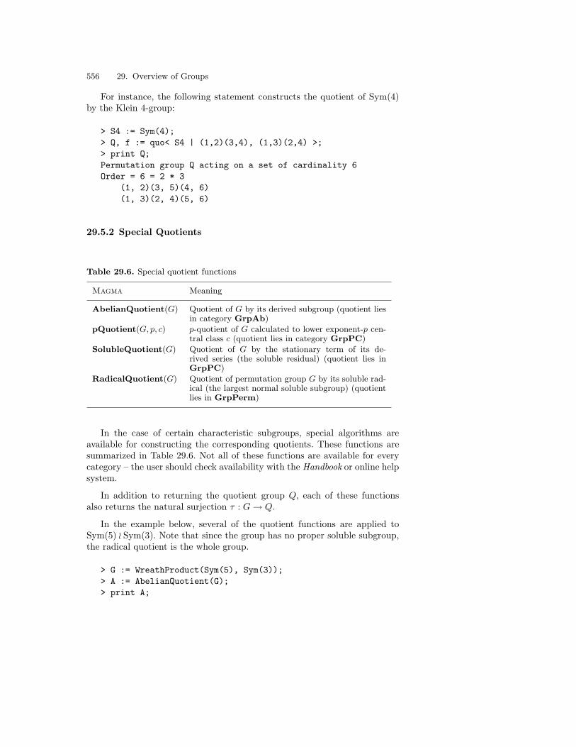
556 29. Overview of Groups
For instance, the following statement constructs the quotient of Sym(4)by the Klein 4-group:
> S4 := Sym(4);> Q, f := quo< S4 | (1,2)(3,4), (1,3)(2,4) >;> print Q;Permutation group Q acting on a set of cardinality 6Order = 6 = 2 * 3
(1, 2)(3, 5)(4, 6)(1, 3)(2, 4)(5, 6)
29.5.2 Special Quotients
Table 29.6. Special quotient functions
Magma Meaning
AbelianQuotient(G) Quotient of G by its derived subgroup (quotient liesin category GrpAb)
pQuotient(G, p, c) p-quotient of G calculated to lower exponent-p cen-tral class c (quotient lies in category GrpPC)
SolubleQuotient(G) Quotient of G by the stationary term of its de-rived series (the soluble residual) (quotient lies inGrpPC)
RadicalQuotient(G) Quotient of permutation group G by its soluble rad-ical (the largest normal soluble subgroup) (quotientlies in GrpPerm)
In the case of certain characteristic subgroups, special algorithms areavailable for constructing the corresponding quotients. These functions aresummarized in Table 29.6. Not all of these functions are available for everycategory – the user should check availability with the Handbook or online helpsystem.
In addition to returning the quotient group Q, each of these functionsalso returns the natural surjection τ : G → Q.
In the example below, several of the quotient functions are applied toSym(5) o Sym(3). Note that since the group has no proper soluble subgroup,the radical quotient is the whole group.
> G := WreathProduct(Sym(5), Sym(3));> A := AbelianQuotient(G);> print A;

29.6 Order and Index Functions 557
Abelian Group isomorphic to Z/2 + Z/2Defined on 2 generatorsRelations:
2*A.1 = 02*A.2 = 0
> B := SolubleQuotient(G);GrpPC : B of order 48 = 2^4 * 3PC-Relations:
B.1^2 = Id(B),B.2^2 = Id(B),B.3^3 = Id(B),B.4^2 = Id(B),B.5^2 = Id(B),B.2^B.1 = B.2 * B.5,B.3^B.1 = B.3^2,B.3^B.2 = B.3 * B.4,B.4^B.1 = B.4 * B.5,B.4^B.3 = B.4 * B.5,B.5^B.3 = B.4
> C := RadicalQuotient(G);> print Order(C) eq Order(G);true
As another example, the pQuotient function applied to the group
〈a, b | a(b,a) = a5, b(a,b) = b5〉constructs a 2-quotient order 2048. The progress of the calculation may bedisplayed by setting the parameter Print to 1:
> G := Group< a, b | a^(b,a) = a^5, b^(a,b) = b^5>;> Q := pQuotient(G, 2, 10 : Print := 1);Lower exponent-2 central series for GGroup: G to lower exponent-2 central class 1 has order 2^2Group: G to lower exponent-2 central class 2 has order 2^5Group: G to lower exponent-2 central class 3 has order 2^8Group: G to lower exponent-2 central class 4 has order 2^10Group: G to lower exponent-2 central class 5 has order 2^11Completed. Lower exponent-2 central class = 5, Order = 2^11
29.6 Order and Index Functions
For a finite group G, one of the most useful invariants is its order. The orderis returned as an integer by the function Order(G), or as a factorization

558 29. Overview of Groups
sequence by the function FactoredOrder(G). If either of these functions isapplied to an infinite matrix group, it will fail.
Care should be exercised when applying the function to an fp-group G,since the order is determined by using the Todd-Coxeter procedure to enu-merate the cosets of the identity subgroup. If G is infinite or has large order,or if the enumeration is difficult, the function may exhaust memory withoutreturning an answer. For this reason, when Order calls the Todd-Coxeterprocedure, it does so with a limit of a million cosets. The user may overridethis limit by calling the Todd-Coxeter function directly.
Similarly, if H is a subgroup of G having finite index, the index [G : H]is returned as an integer by the function Index(G,H) or as a factorizationsequence by the function FactoredIndex(G,H).
The index functions may only be applied to matrix groups for which aBSGS can be computed (see Section ??). In practice, this requires that thematrix group be finite and defined over either a field or a euclidean ring.
The example below uses the GLSyl function defined above to constructthe Sylow 2-subgroup of GL(3, 8), and then applies order and index functions:
> G := GeneralLinearGroup(3, GF(8));> print Order(G);115379712> print FactoredOrder(G);[ <2, 9>, <3, 2>, <7, 3>, <73, 1> ]> T := GLSyl(G);> print FactoredOrder(T);[ <2, 9> ]> print Index(G, T);225351> print FactoredIndex(G, T);[ <3, 2>, <7, 3>, <73, 1> ]
Another useful numerical invariant of a group is its exponent, that is, thelowest-common multiple of the orders of its elements. The Magma functionExponent(G) computes the exponent of a group G for which a SNF iscomputable. For example, when applied to the group GL(3, 8) above, it givesthe answer 18 396.

29.7 Properties of Groups and Subgroups 559
29.7 Properties of Groups and Subgroups
The functions listed in Table 29.7 determine abstract properties of a group.Note that, with the exception of the function IsPerfect, these functions arenot applicable to fp-groups.
Table 29.7. Some tests on properties of a group
IsAbelian(G) IsElementaryAbelian(G)
IsNilpotent(G) IsPerfect(G)
IsCyclic(G) IsSimple(G)
IsSpecial(G) IsExtraSpecial(G)
IsSoluble(G), IsSolvable(G)
There are also functions which test properties relating to the way in whicha subgroup H or pair of subgroups H and K are embedded in group G.Table 29.8 lists some of them.
Table 29.8. Some tests on properties of a subgroup
IsConjugate(G, H, K) IsNormal(G, H)
IsSubnormal(G, H) IsSelfNormalizing(G, H)
IsCentral(G, H) IsMaximal(G, H)
29.8 Characteristic Subgroups, Series and NormalStructure
29.8.1 Characteristic Subgroups
Magma provides functions for determining the standard characteristic sub-groups, as listed in Table 29.9. All but one of these functions require a SNF forthe group G; the only exception is that DerivedSubgroup may be appliedto an fp-group. Furthermore, note that the functions Agemo and Omegaare only defined for p-groups, while FrattiniSubgroup is only implementedfor p-groups.
The example below applies some of these functions to the soluble primitivegroup gp9 introducted above:

560 29. Overview of Groups
Table 29.9. Characteristic subgroups
Magma Meaning
Centre(G) Centre of G
Hypercentre(G) Stationary term of upper central series of G
DerivedSubgroup(G) Derived subgroup of G
FittingSubgroup(G) Maximal normal nilpotent subgroup of G
FrattiniSubgroup(G) Intersection of maximal subgroups of p-group G
Radical(G) Maximal normal soluble subgroup of G
SolubleResidual(G) Stationary term of derived series
Agemo(G, i) Subgroup of p-group G generated by the pi-thpowers
Omega(G, i) Subgroup of p-group G generated by the elementsof order dividing pi
> gp9 := PermutationGroup< 9 | (1,2,3,4)(5,6,7,8),(1,8)(3,6)(5,7), (1,4,7)(2,3,5)(6,9,8) >;
> print Centre(gp9);Permutation group acting on a set of cardinality 9Order = 1
Id($)> print Hypercentre(gp9);Permutation group acting on a set of cardinality 9Order = 1
Id($)> print DerivedSubgroup(gp9);Permutation group acting on a set of cardinality 9Order = 36 = 2^2 * 3^2
(1, 8, 3, 6)(2, 7, 4, 5)(1, 3, 9)(2, 6, 7)(4, 5, 8)
> print FittingSubgroup(gp9);Permutation group acting on a set of cardinality 9Order = 9 = 3^2
(1, 8, 2)(3, 4, 6)(5, 7, 9)(1, 7, 4)(2, 5, 3)(6, 8, 9)
> print Radical(gp9);Permutation group acting on a set of cardinality 9Order = 144 = 2^4 * 3^2
(2, 5)(4, 7)(6, 8)(1, 8, 2)(3, 4, 6)(5, 7, 9)(2, 4, 8, 7)(3, 6, 9, 5)(1, 7, 4)(2, 5, 3)(6, 8, 9)(2, 5, 8, 6)(3, 4, 9, 7)

29.8 Characteristic Subgroups, Series and Normal Structure 561
(2, 8)(3, 9)(4, 7)(5, 6)> SolubleResidual(gp9);Permutation group acting on a set of cardinality 9Order = 1
Id($)
29.8.2 Series
Table 29.10 lists the Magma functions creating various series of characteristicsubgroups (as a sequence of subgroups). They are applicable only to groupsfor which a SNF can be computed, so none of them are available for fp-groups. Moreover, certain of the series are only defined for p-groups or solublegroups, while not all of the functions are available for all categories of groupspossessing SNFs.
Table 29.10. Series
Magma Meaning
ChiefSeries(G) Chief series for G
CompositionSeries(G) Composition series for G
ElementaryAbelianSeries(G) Series G = E0 ¤ E1 ¤ · · · ¤ Er, whereEi/Ei−1 is elementary abelian (G must besoluble)
DerivedSeries(G) Series G = G(0) ¤ G1 ¤ G2 ¤ · · · , whereG(i) = [G(i−1), G(i−1)]
DerivedLength(G) If G is soluble, returns least integer l suchthat G(l) is trivial; else returns number ofterms up to and including stationary term
JenningsSeries(G) Series G = J1 ¤J2 ¤J3 ¤ · · · , where Ji+1 =〈(Ji, G), Jp
k 〉 with k = d(i + 1)/pe (G mustbe a p-group)
LowerCentralSeries(G) Series G = G1 ¤G2 ¤G3 ¤ · · · , where Gi =[Gi−1, G]
NilpotencyClass If G is nilpotent, returns least integer c suchthat term Gc of lower central series is triv-ial; else returns −1
pCentralSeries(G, p) Series G = P1¤P2¤P3¤ · · · , where Pi−1 =[G, Pi]Pi (G must be soluble and prime pmust divide |G|
SubnormalSeries(G, H) Series N1 = H ¢ N2 ¢ . . . ¢ Nr = G, whereH is a subgroup of G
UpperCentralSeries(G) Series Z0 = 1, Zi/Zi−1 = Z(G/Zi−1)
For example:

562 29. Overview of Groups
> gp9 := PermutationGroup< 9 | (1,2,3,4)(5,6,7,8),(1,8)(3,6)(5,7), (1,4,7)(2,3,5)(6,9,8) >;
> print ChiefSeries(gp9);[
Permutation group gp9 acting on a set of cardinality 9Order = 144 = 2^4 * 3^2
(1, 2, 3, 4)(5, 6, 7, 8)(1, 8)(3, 6)(5, 7)(1, 4, 7)(2, 3, 5)(6, 9, 8),
Permutation group acting on a set of cardinality 9Order = 72 = 2^3 * 3^2
(3, 7)(4, 9)(5, 6)(2, 8)(3, 4)(7, 9)(2, 6)(3, 9)(5, 8)(1, 7, 4)(2, 5, 3)(6, 8, 9),
Permutation group acting on a set of cardinality 9Order = 9 = 3^2
(1, 8, 2)(3, 4, 6)(5, 7, 9)(1, 7, 4)(2, 5, 3)(6, 8, 9),
Permutation group acting on a set of cardinality 9Order = 1
Id($)]> print DerivedSeries(gp9);print DS;[
Permutation group gp9 acting on a set of cardinality 9Order = 144 = 2^4 * 3^2
(1, 2, 3, 4)(5, 6, 7, 8)(1, 8)(3, 6)(5, 7)(1, 4, 7)(2, 3, 5)(6, 9, 8),
Permutation group acting on a set of cardinality 9Order = 36 = 2^2 * 3^2
(1, 6, 3, 8)(2, 5, 4, 7)(2, 5, 8, 6)(3, 4, 9, 7)(1, 7, 2, 3)(4, 6, 5, 9),
Permutation group acting on a set of cardinality 9Order = 9 = 3^2
(1, 5, 6)(2, 9, 4)(3, 8, 7)(1, 7, 4)(2, 5, 3)(6, 8, 9),
Permutation group acting on a set of cardinality 9Order = 1
Id($)]
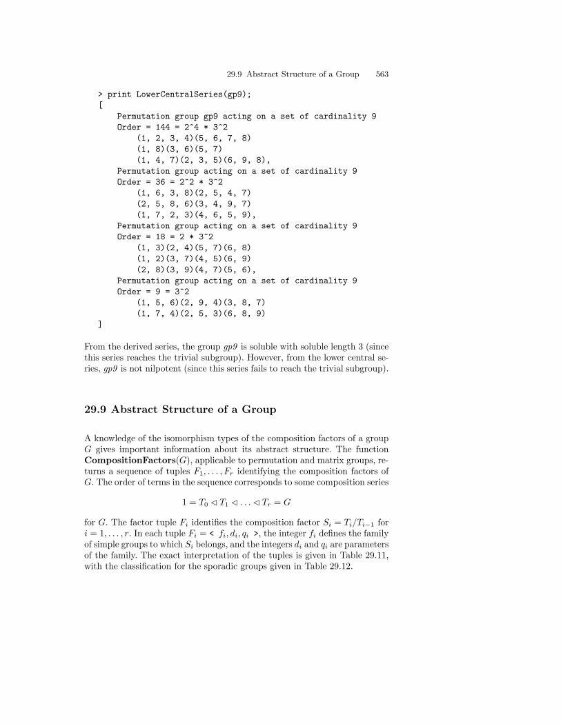
29.9 Abstract Structure of a Group 563
> print LowerCentralSeries(gp9);[
Permutation group gp9 acting on a set of cardinality 9Order = 144 = 2^4 * 3^2
(1, 2, 3, 4)(5, 6, 7, 8)(1, 8)(3, 6)(5, 7)(1, 4, 7)(2, 3, 5)(6, 9, 8),
Permutation group acting on a set of cardinality 9Order = 36 = 2^2 * 3^2
(1, 6, 3, 8)(2, 5, 4, 7)(2, 5, 8, 6)(3, 4, 9, 7)(1, 7, 2, 3)(4, 6, 5, 9),
Permutation group acting on a set of cardinality 9Order = 18 = 2 * 3^2
(1, 3)(2, 4)(5, 7)(6, 8)(1, 2)(3, 7)(4, 5)(6, 9)(2, 8)(3, 9)(4, 7)(5, 6),
Permutation group acting on a set of cardinality 9Order = 9 = 3^2
(1, 5, 6)(2, 9, 4)(3, 8, 7)(1, 7, 4)(2, 5, 3)(6, 8, 9)
]
From the derived series, the group gp9 is soluble with soluble length 3 (sincethis series reaches the trivial subgroup). However, from the lower central se-ries, gp9 is not nilpotent (since this series fails to reach the trivial subgroup).
29.9 Abstract Structure of a Group
A knowledge of the isomorphism types of the composition factors of a groupG gives important information about its abstract structure. The functionCompositionFactors(G), applicable to permutation and matrix groups, re-turns a sequence of tuples F1, . . . , Fr identifying the composition factors ofG. The order of terms in the sequence corresponds to some composition series
1 = T0 ¢ T1 ¢ . . . ¢ Tr = G
for G. The factor tuple Fi identifies the composition factor Si = Ti/Ti−1 fori = 1, . . . , r. In each tuple Fi = < fi, di, qi >, the integer fi defines the familyof simple groups to which Si belongs, and the integers di and qi are parametersof the family. The exact interpretation of the tuples is given in Table 29.11,with the classification for the sporadic groups given in Table 29.12.

564 29. Overview of Groups
Table 29.11. Group families for CompositionFactors
f Family name f Family name
1 A(d, q) 11 2B(2, q)
2 B(d, q) 12 2D(d, q)
3 C(d, q) 13 3D(4, q)
4 D(d, q) 14 2G(2, q)
5 G(2, q) 15 2F(4, q)
6 F(4, q) 16 2E(6, q)
7 E(6, q) 17 Alternating(d)
8 E(7, q) 18 Sporadic group - see Table 29.12
9 E(8, q) 19 Cyclic(q)
10 2A(d, q)
Table 29.12. Sporadic groups for CompositionFactors
d Group name d Group name d Group name
1 M11 10 SUZ 19 LY
2 M12 11 J3 20 RU
3 M22 12 CO1 21 ON
4 M23 13 CO2 22 TH
5 M24 14 CO3 23 HA
6 J1 15 HE 24 BM
7 HS 16 M(22) 25 M
8 J2 17 M(23) 26 J4
9 MCL 18 M(24)
For example, consider the problem of determining the structure of thegroup G of 9× 9 matrices generated by these matrices over GF(3):
2 2 0 0 0 0 0 0 02 2 1 0 0 0 0 0 00 1 1 0 0 0 0 0 00 0 0 0 1 2 0 0 00 0 0 2 1 0 0 0 00 0 0 2 2 1 0 0 00 0 0 0 0 0 1 0 00 0 0 0 0 0 0 1 00 0 0 0 0 0 0 0 1
0 0 0 1 0 0 0 0 00 0 0 0 1 2 0 0 00 0 0 2 1 1 0 0 01 2 0 0 0 0 0 0 00 0 2 0 0 0 0 0 02 2 2 0 0 0 0 0 00 0 0 0 0 0 1 0 00 0 0 0 0 0 0 1 00 0 0 0 0 0 0 0 1
It may be solved in Magma as follows:

29.9 Abstract Structure of a Group 565
To perform this example online, type load "I96c29e2";
> G := MatrixGroup<9, GF(3) |> [ 2, 2, 0, 0, 0, 0, 0, 0, 0,> 2, 2, 1, 0, 0, 0, 0, 0, 0,> 0, 1, 1, 0, 0, 0, 0, 0, 0,> 0, 0, 0, 0, 1, 2, 0, 0, 0,> 0, 0, 0, 2, 1, 0, 0, 0, 0,> 0, 0, 0, 2, 2, 1, 0, 0, 0,> 0, 0, 0, 0, 0, 0, 1, 0, 0,> 0, 0, 0, 0, 0, 0, 0, 1, 0,> 0, 0, 0, 0, 0, 0, 0, 0, 1 ],> [ 0, 0, 0, 1, 0, 0, 0, 0, 0,> 0, 0, 0, 0, 1, 2, 0, 0, 0,> 0, 0, 0, 2, 1, 1, 0, 0, 0,> 1, 2, 0, 0, 0, 0, 0, 0, 0,> 0, 0, 2, 0, 0, 0, 0, 0, 0,> 2, 2, 2, 0, 0, 0, 0, 0, 0,> 0, 0, 0, 0, 0, 0, 1, 0, 0,> 0, 0, 0, 0, 0, 0, 0, 1, 0,> 0, 0, 0, 0, 0, 0, 0, 0, 1 ] >;> cf := CompositionFactors(G);> // 2-dimensional layout> print cf;
G| Cyclic(2)*| A(2, 3) = L(3, 3)*| A(2, 3) = L(3, 3)*| Cyclic(2)*| Cyclic(2)1
> // show tuples in cf> for i in [1..#cf] do print cf[i]; end for;<19, 0, 2><1, 2, 3><1, 2, 3><19, 0, 2><19, 0, 2>
The items in the middle of the chain indicate the proper subgroups of a com-position series for G. The isomorphism type of the corresponding composition

566 29. Overview of Groups
factor is indicated on the right. It can be seen that the group has a solublequotient isomorphic to the cyclic group of order 2. After this, there are twocopies of PSL(3, 3) sitting above an abelian group of order 4.
If G is known to be a simple group, the function NameSimple(G) returnsa tuple identifying G according to the conventions described above.
29.10 Conjugacy Classes of Elements
The three major issues concerning the conjugacy classes of elements of agroup G are:
– to determine whether two elements are conjugate in G;
– to determine the classes of G, in the sense of constructing a representativeand basic invariants for each class;
– having determined these classes, to determine quickly the class in which agiven element of G falls.
These problems will be considered in turn.
29.10.1 Testing Conjugacy
If x and y are elements of a group G, the function IsConjugate(G, x, y) testswhether x and y are conjugate in G. If x and y are conjugate, the functionreturns as its second value, an element g such that xg = y.
MUST FIND A DIFFERENT EXAMPLE. THIS IS USED EXTEN-SIVELY IN Iperm.tex
For instance, the group below is is the group of symmetries of a cube:
> cube<a, b, c> := PermutationGroup< 8 |> (1, 2, 3, 4)(5, 6, 7, 8), (2, 4, 5)(3, 8, 6),> (1, 5)(2, 6)(3, 7)(4, 8) >;> conj, z := IsConjugate(cube, b, b^-1);> print conj;true> print z;(3, 6)(4, 5)
If it is necessary to determine for a large number of elements the conjugacyclass to which they belong, it may be more efficient to use the functionClassMap (Section 29.10.4).

29.10 Conjugacy Classes of Elements 567
29.10.2 Constructing One Class
The set of conjugates of x under the action of the subgroup H is given byClass(H, x) or Conjugates(H, x). If the value of H is set to G, the functionwill return the entire conjugacy class of x. For example, calculations aboveshowed that b−1 lies in the same class as b. The statement below confirmsthis, by displaying the entire conjugacy class of b (including b−1):
> print Class(cube, b);
(1, 6, 8)(2, 7, 4),(1, 3, 6)(4, 7, 5),(1, 6, 3)(4, 5, 7),(2, 4, 5)(3, 8, 6),(1, 8, 6)(2, 4, 7),(1, 8, 3)(2, 5, 7),(2, 5, 4)(3, 6, 8),(1, 3, 8)(2, 7, 5)
Since Class(H, x) and Conjugates(H, x) return the class containing theelement x as an enumerated set. Consequently, this function should notbe used on large classes. If the user merely needs to know the size ofthe class containing x, it is much more efficient to use the expressionIndex(G,Centralizer(G, x).
29.10.3 Constructing All the Classes
Let K1, . . . ,Kr denote the conjugacy classes of G. For the purposes of thisdiscussion, constructing the classes of G will be taken to mean determining,for each class Ki a representative element xi and the cardinality of Ki (thelength of the class).
The function ConjugacyClasses(G) or Classes(G) constructs all theconjugacy classes in the group G. It does not return the classes as such; itmerely returns sufficient information about each class so that the user caneasily compute an entire class if it is wanted explicitly. The return value ofClasses(G) is a sequence of tuples, one tuple for each conjugacy class; thecomponents of each tuple are the order of the elements in that class, thelength of the class, and a representative element for the class.
Individual entries of this sequence should be treated by the user as normaltuples. However, when the whole classes sequence is printed, there is a specialdisplay format provided for the convenience of the user:

568 29. Overview of Groups
> cubecl := Classes(cube);> cl9info := cubecl[9]; // information on class 9> print cl9info;<4, 6, (1, 3, 8, 6)(2, 4, 7, 5)>> print cl9info[2]; // length of class 96> print cubecl[4, 1]; // order of class 42
> // special display format> print cubecl;Conjugacy Classes of group cube-------------------------------[1] Order 1 Length 1
Rep Id(cube)
[2] Order 2 Length 1Rep (1, 7)(2, 8)(3, 5)(4, 6)
[3] Order 2 Length 3Rep (1, 3)(2, 4)(5, 7)(6, 8)
[4] Order 2 Length 3Rep (1, 2)(3, 4)(5, 6)(7, 8)
[5] Order 2 Length 6Rep (1, 7)(2, 3)(4, 6)(5, 8)
[6] Order 2 Length 6Rep (3, 6)(4, 5)
[7] Order 3 Length 8Rep (1, 8, 3)(2, 5, 7)
[8] Order 4 Length 6Rep (1, 2, 3, 4)(5, 6, 7, 8)
[9] Order 4 Length 6Rep (1, 3, 8, 6)(2, 4, 7, 5)
[10] Order 6 Length 8Rep (1, 2, 3, 7, 8, 5)(4, 6)

29.10 Conjugacy Classes of Elements 569
To illustrate how one may loop through the classes sequence, the classequation, which states that the order of a group G equals
∑[G : CG(x)],
where x ranges over the class representatives, will be verified for cube:
> print Order(cube);48> print &+[Index(cube, Centralizer(cube, cl[3])) :> cl in cubecl];48
The determination of classes is known to be a hard problem. Severalalgorithms are available in Magma. A particular algorithm may be selectedby means of an Al parameter on the Classes function. The value "Action"will invoke an algorithm that finds the classes by computing the orbits ofthe elements of G under conjugation by G. Consequently, it is only useful forsmall groups but in some cases it will be faster than the alternative methods.The value "Random" specifies a random algorithm which attempts to locate anelement in each conjugacy class. Finally, the Al value "Extension" employsan inductive algorithm that computes classes in a sequence of successivelylarger quotients of G determined by an elementary abelian series for G.
Finally, if the user already knows a set of representatives for the classes,the AssertAttribute command may be used to define a value for the"Classes" attribute for the group, by giving the classes in the form of asequence containing exactly one representative from each conjugacy class,
29.10.4 The Class Map and Power Map
For certain applications (such as constructing a class matrix) it is necessary toidentify the class to which each member of a large set of elements belongs. LetR = [x1, . . . , xr] be the sequence of class representatives for G constructed bythe Class function. Let f : G → R be defined by f(x) = xi where x belongsto the class having representative xi. The mapping f is called the class mapof G and may be created by the function ClassMap(G). The function pre-computes certain information in addition to the class representatives, whichmay greatly speed up the identification of the class representative for x. Notethat if the classes are not known at the time ClassMap(G) is invoked, theywill be first computed.
A function related to ClassMap is ClassRepresentative(G, x). It re-turns the class representative of x, that is, the representative for the classcontaining x that appears in the sequence of tuples returned by Classes.

570 29. Overview of Groups
For example, the Magma code below calculates that b lies in the classnumbered seven by the Class function, and verifies that the class represen-tative of b is the representative for the seventh class:
> cmcube := ClassMap(cube);> print cmcube;Mapping from: GrpPerm: cube to 1 .. 10 > print cmcube(b);7> print cubecl[7, 3] eq ClassRepresentative(cube, b);true
The mapping f returned by ClassMap may be applied not only to individualelements of G but also to sets and sequences of elements of G:
> print cmcube([b, c, b*c]);[ 7, 4, 10 ]
Suppose the conjugacy classes of G are denoted K1, . . . ,Kr. If t is a fixedpositive integer, and Ki is a class of G, there exists a unique class Kj suchthat xt : x ∈ Ki ⊆ Kj . The behaviour of the classes of G under the takingof powers may be represented by a mapping known as the powermap φ. Thepowermap may be defined formally as follows: Let C = 1, . . . , r denote theset of indices of the classes and suppose the exponent of G is e. The powermap φ for G is the mapping φ : C × 1, . . . , r → C where φ(i, j) is theindex of the class containing xj
i (xi is a representative for Ki). This mapis created by the function PowerMap(G). If the class map is not alreadyknown, PowerMap will cause it to be created.
The use of the power map is illustrated by displaying how the classes ofcube are mapped under the taking of squares, cubes and fouth powers.
> phi := PowerMap(cube);> print [ phi(i, 2) : i in [1..#cubecl] ];[ 1, 1, 1, 1, 1, 1, 7, 3, 3, 7 ]> print [ phi(i, 3) : i in [1..#cubecl] ];[ 1, 2, 3, 4, 5, 6, 1, 8, 9, 2 ]> print [ phi(i, 4) : i in [1..#cubecl] ];[ 1, 1, 1, 1, 1, 1, 7, 1, 1, 7 ]
Thus, inspecting the cubes, it can be seen that the cubes of the elementsof class 10 fall into class 2.
For each class Ki of G defineKi =∑
x, where x runs through the elementsof Ki. It is a standard result from representation theory that the formal sums

29.11 Conjugacy Classes of Subgroups 571
Ki, i = 1, . . . , r form a basis for the centre of the group algebra C[G]. Thus,the product of any two class sums can be written as follows:
KiKj =∑
cijkKk
where the sum is over k. The structure constants cijk correspond to thenumber of solutions (x, y) of the equation xy = z, where z ∈ Kk is fixed andx ∈ Ki, y ∈ Kj . The matrix Mi, whose (j, k)th entry is cijk, is called thestructure constant matrix for class i. It may be computed using the functionClassMatrix(G, i) as shown in the following example in which the classmatrix for cube for the unique conjugacy class of elements of order 3 (class7) is computed.
> print ClassMatrix(cube, 7);[0 0 0 0 0 0 1 0 0 0][0 0 0 0 0 0 0 0 0 1][0 0 0 0 0 0 3 0 0 0][0 0 0 0 0 0 0 0 0 3][0 0 0 0 4 0 0 4 0 0][0 0 0 0 0 4 0 0 4 0][8 0 8 0 0 0 4 0 0 0][0 0 0 0 4 0 0 4 0 0][0 0 0 0 0 4 0 0 4 0][0 8 0 8 0 0 0 0 0 4]
The matrix may be interpreted as follows: Consider row 6 of the matrix. Ifthe elements of class 7 are multiplied by an element from class 6, then fourof the products belong to class 6 and four belong to class 9 as is seen fromthe calculation below (phi is the power map defined above).
> x := cubecl[6][3];> [ phi(x*y) : y in Class(cube, cubecl[7][3]) ];[ 9, 6, 6, 9, 6, 9, 6, 9 ]
29.11 Conjugacy Classes of Subgroups
29.11.1 Determining the Conjugacy Classes
Knowledge of the conjugacy classes of subgroups of a group G provides adetailed picture of the internal structure of G. Because of the huge numberof subgroups that a complicated group may possess, it is only practical to findall conjugacy classes of subgroups in groups that either have moderate order

572 29. Overview of Groups
or relatively few classes of subgroups. The algorithm employed by Magma forpermutation or matrix groups is restricted to groups whose radical quotient(i.e., quotient by the maximal normal soluble subgroup) is less than somebound (20, 160 at the time of writing, but to be increased).
The basic function, SubgroupClasses(G), determines a representativesubgroup for each conjugacy class. The subgroups are returned as a sequenceof records where the ith record contains:
1. A representative subgroup H for the ith conjugacy class (field name:subgroup);
2. The order of the subgroup (field name: order);
3. The number of subgroups in the class (field name: length);
4. (Optional, and only relevant for permutation groups) A presentation forH (field name presentation).
The function is illustrated by computing the subgroups of Alt(5):
> G := Alt(5);> S := SubgroupClasses(G);> print S;Conjugacy classes of subgroups------------------------------
[ 1] Order 1 Length 1Permutation group acting on a set of cardinality 5
Id($)[ 2] Order 2 Length 15
Permutation group acting on a set of cardinality 5(1, 4)(3, 5)
[ 3] Order 3 Length 10Permutation group acting on a set of cardinality 5
(1, 3, 2)[ 4] Order 5 Length 6
Permutation group acting on a set of cardinality 5(1, 4, 3, 5, 2)
[ 5] Order 4 Length 5Permutation group acting on a set of cardinality 5
(1, 4)(3, 5)(1, 5)(3, 4)
[ 6] Order 6 Length 10Permutation group acting on a set of cardinality 5
(1, 3, 2)(2, 3)(4, 5)
[ 7] Order 10 Length 6Permutation group acting on a set of cardinality 5
(1, 4, 3, 5, 2)(1, 4)(2, 3)
[ 8] Order 12 Length 5

29.11 Conjugacy Classes of Subgroups 573
Permutation group acting on a set of cardinality 5(1, 4)(3, 5)(3, 4, 5)
[ 9] Order 60 Length 1Permutation group acting on a set of cardinality 5
(1, 4)(3, 5)(1, 3, 2)
It can be seen that Alt(5) has 9 conjugacy classes of subgroups. Class 6consists of a class containing 10 subgroups of order 6. The chosen represen-tative for this class is the subgroup generated by the permutations (1, 3, 2)and (2, 3)(4, 5).
Since the function returns a sequence, it is an easy matter to iterate overthe subgroup classes. This is illustrated by determining the orders of thenon-abelian simple subgroups of the Mathieu group M12:
> m12 := PermutationGroup< 12 |> (1, 11, 5, 2, 8, 3, 9, 7, 4, 10, 12),> (1, 8, 12, 9, 6)(2, 4, 10, 11, 3) >;> print Order(12);95040> S := SubgroupClasses(G);> print [ <i, Order(sub)> : i in [1..#S] |> not IsAbelian(sub) and IsSimple(sub)> where sub := S[i]‘subgroup ];[ <90, 60>, <91, 60>, <92, 60>, <93, 60>, <119, 660>,<120, 660>, <131, 360>, <132, 360>, <145, 7920>,<146, 7920>, <147, 95040> ]
Table 29.13. Restriction parameters for subgroup functions
Parameter Meaning
OrderEqual If assigned integer n, only construct subgroups of order n
OrderDividing If assigned integer n, only construct subgroups having orderdividing n
IsNormal If assigned true, only construct normal subgroups
IsRegular If assigned true, only construct regular subgroups (for per-mutation groups only)
Additional restrictions on the subgroups constructed may be imposed bymeans of the parameters shown in Table 29.13. These parameters apply toall of the subgroup functions listed above, including SubgroupClasses.

574 29. Overview of Groups
The central algorithm for computing the subgroup classes allows variousrestrictions to be imposed on the kind of subgroups that are constructed.Different versions of the subgroup function allow the user to construct specificsubgroup varieties of subgroups. These varieties are displayed in Table 29.14.
Table 29.14. Varieties of subgroups
ElementaryAbelianSubgroups(G) AbelianSubgroups(G)
NilpotentSubgroups(G) SolubleSubgroups(G)
PerfectSubgroups(G) SimpleSubgroups(G)
RegularSubgroups(G)
These functions will be used to determine the conjugacy classes of ele-mentary abelian subgroups of order 16 in the group Z/2Z oAlt(5):
> G := WreathProduct(CyclicGroup(GrpPerm, 2), Alt(5));> #G;1920> S := ElementaryAbelianSubgroups(G: OrderEqual := 16);> print #S;7
29.11.2 The Poset of Subgroup Classes
In addition to finding representatives for conjugacy classes of subgroups,Magma allows the user to create the poset L of subgroup classes. The el-ements of the poset correspond to the conjugacy classes of subgroups. Twolattice elements a and b are joined by an edge if either some subgroup of theconjugacy class a is a maximal subgroup of some subgroup of conjugacy classb or vice-versa. The elements of L are called subgroup-poset elements and arenumbered from 1 to n, where n is the cardinality of L. Various functionsallow the user to identify maximal subgroups, normalizers, centralizers etc inthe lattice. Given e ∈ L, it is possible to create the subgroup H of G corre-sponding to e, and to create the element of L corresponding to a subgroupof G.
If a large number of poset operations are to be performed, it may be moreefficient to construct the complete subgroup class poset first.
The function SubgroupLattice(G) determines the conjugacy classes ofsubgroups and the builds the poset data structure. The construction of theposet can be very time-consuming and should only be used with care. Thefunction has the following Boolean-valued parameters: Properties – if true,
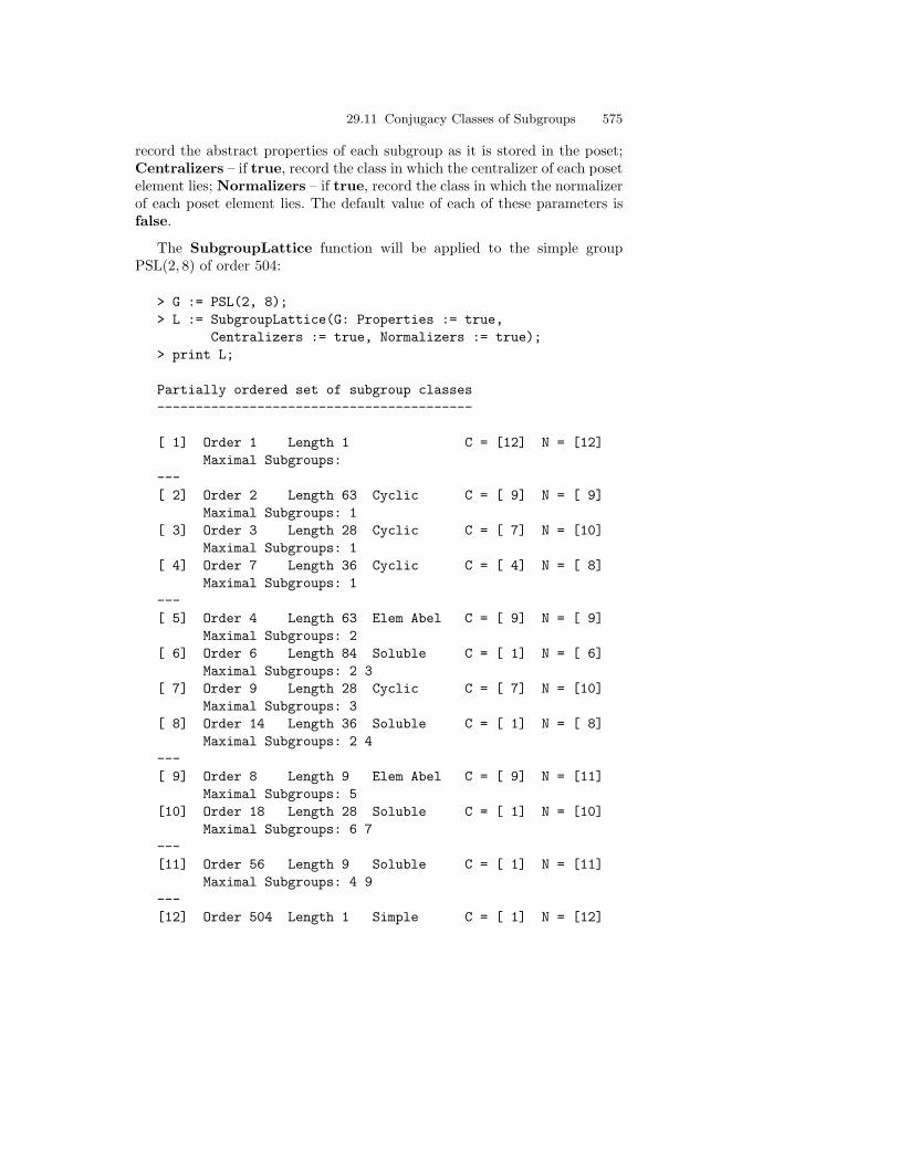
29.11 Conjugacy Classes of Subgroups 575
record the abstract properties of each subgroup as it is stored in the poset;Centralizers – if true, record the class in which the centralizer of each posetelement lies; Normalizers – if true, record the class in which the normalizerof each poset element lies. The default value of each of these parameters isfalse.
The SubgroupLattice function will be applied to the simple groupPSL(2, 8) of order 504:
> G := PSL(2, 8);> L := SubgroupLattice(G: Properties := true,
Centralizers := true, Normalizers := true);> print L;
Partially ordered set of subgroup classes-----------------------------------------
[ 1] Order 1 Length 1 C = [12] N = [12]Maximal Subgroups:
---[ 2] Order 2 Length 63 Cyclic C = [ 9] N = [ 9]
Maximal Subgroups: 1[ 3] Order 3 Length 28 Cyclic C = [ 7] N = [10]
Maximal Subgroups: 1[ 4] Order 7 Length 36 Cyclic C = [ 4] N = [ 8]
Maximal Subgroups: 1---[ 5] Order 4 Length 63 Elem Abel C = [ 9] N = [ 9]
Maximal Subgroups: 2[ 6] Order 6 Length 84 Soluble C = [ 1] N = [ 6]
Maximal Subgroups: 2 3[ 7] Order 9 Length 28 Cyclic C = [ 7] N = [10]
Maximal Subgroups: 3[ 8] Order 14 Length 36 Soluble C = [ 1] N = [ 8]
Maximal Subgroups: 2 4---[ 9] Order 8 Length 9 Elem Abel C = [ 9] N = [11]
Maximal Subgroups: 5[10] Order 18 Length 28 Soluble C = [ 1] N = [10]
Maximal Subgroups: 6 7---[11] Order 56 Length 9 Soluble C = [ 1] N = [11]
Maximal Subgroups: 4 9---[12] Order 504 Length 1 Simple C = [ 1] N = [12]

576 29. Overview of Groups
Maximal Subgroups: 8 10 11
From the poset L of subgroup classes of PSL(2, 8), it can be seen, for ex-ample, that class 7 contains 28 subgroups of order 9. These are cyclic, theirnormalizers lie in class 11, and their maximal subgroups belong to class 3.
The term class will be used in the remainder of this section when refer-ring to poset elements. If G has r conjugacy classes of subgroups, the posetelements (classes) are indexed by the integers 1 to r. Indeed, a poset elementis represented by this integer for input and output purposes. So if L is sucha poset, the coercion L!i will denote the ith class of the poset. Operationson subgroup posets are shown in Table 29.15.
Table 29.15. General subgroup poset operations
Magma Meaning
#L Number of conjugacy classes of subgroups
L!i ith element (class) of the poset
Z!i Integer corresponding to poset e, where Z is integer ring
L!H Element of the poset containing subgroup H
Bottom(L) Trivial subgroup class
Top(L) Class corresponding to G
The standard relational operations for poset elements are denoted by eq,ne, ge, gt, le, and lt. For instance, the value of e ge f is true if the class econtains class f .
Table 29.16. Extracting information from a subgroup poset
Magma Meaning
Group(e) Representative for class e
Centralizere, f) Class containing centralizers of f in e
Normalizer(e, f) Class containing normalizers of f in e
Length(e) Number of subgroups in class e
Order(e) Order of subgroups in class e
MaximalSubgroups(e) Classes containing maximal subgroups of e
MinimalOvergroups(e, f) Classes containing minimal overgroups of e
NumberOfInclusions(e, f) Number of subgroups of the class e lying in afixed representative of the class f

29.11 Conjugacy Classes of Subgroups 577
The following code constructs a chain from the bottom to the top of thesubgroup classes poset for PSL(2, 8) displayed above and then prints theindices of successive terms of the chain:
> H := Bottom(L);> C := [H];> while H ne Top(L) do> H := Representative(MinimalOvergroups(H));> C := Append(C, H);> end while;> print C;[ 1, 2, 5, 9, 11, 12 ]> print [ Order(C[i+1]) div Order(C[i]) : i in [1..#C-1]];[ 2, 2, 2, 7, 9 ]
The Burnside matrix of a subgroup lattice displays information about thecontainment relationship between all pairs of conjugacy classes of subgroups.This matrix is of some interest to combinatorial theorists. In what follows itwill be assumed that L is a subgroup poset for the group G. Let S1, . . . , Sn
denote the conjugacy classes of subgroups corresponding to the elements ofL, where S1 is the trivial subgroup. For each class Si, where i = 1, . . . , n,let si be the number of subgroups in Si and let ri denote the representativesubgroup for the class Si. For i, j ∈ 1, . . . , n, define bij to be the numberof subgroups in class Si which either contain rj or are contained in rj . Thematrix (bij) will be termed the Burnside matrix of the subgroup poset Land it may be displayed using the function PrintBurnsideMatrix(L). Theexample below displays the Burnside matrix for PSL(2, 8):
> PrintBurnsideMatrix(L);
CL ORD 1 2 3 4 5 6 7 8 9 10 11 12
1 1 1 1 1 1 1 1 1 1 1 1 1 12 2 63 1 . . 3 3 . 7 7 9 7 633 3 28 . 1 . . 1 1 . . 1 . 284 7 36 . . 1 . . . 1 . . 8 365 4 63 3 . . 1 . . . 7 . 7 636 6 84 4 3 . . 1 . . . 3 . 847 9 28 . 1 . . . 1 . . 1 . 288 14 36 4 . 1 . . . 1 . . . 369 8 9 1 . . 1 . . . 1 . 1 9
10 18 28 4 1 . . 1 1 . . 1 . 2811 56 9 1 . 2 1 . . . 1 . 1 912 504 1 1 1 1 1 1 1 1 1 1 1 1

578 29. Overview of Groups
29.11.3 Normal Subgroups
Current techniques for finding all normal subgroups are restricted in their ap-plication to groups of moderate order. The function NormalSubgroups(G)returns the normal subgroups of G as a sequence of records having the sameformat as the subgroup records returned by SubgroupClasses. For instance:
> G := WreathProduct(Sym(3), Sym(5));> print #G;933120> N := NormalSubgroups(G);> print [ r‘order : r in N ];[ 1, 243, 486, 3888, 7776, 233280, 466560, 466560,466560, 933120 ]
It can be seen that G has 8 proper normal subgroups.
In the case of permutation groups and matrix groups, the functionMinimalNormalSubgroups(G) finds the minimal normal subgroups of G.When G is a primitive permutation group, this function is quite efficient, butfor other groups, a naive algorithm is employed.
29.12 Characters
29.12.1 Class Functions and Characters
Let K be a field and G be a group. A representation of G is a homomorphismψ : G → GL(n,K), for some positive integer n. The character of G affordedby the representation ψ is the mapping χ : G → K defined by χ : g → Trψ(g).An irreducible character is afforded by an irreducible representation.
In this section, K will be taken to be the complex field C. Over C, a finitegroup possesses a finite number k of irreducible representations, where k isthe number of conjugacy classes of G.
A class function on a group G is a mapping φ : G →C. The set of classfunctions on G forms a vector space W over C having dimension k, where theirreducible characters for G constitute a basis. The standard inner productof characters makes W an inner product space. The set of distinct irreduciblecharacters over C of G will be written as Irr(G).
For both theoretical and computational purposes, it is convenient to workin the space W of class functions. The function ClassFunctionSpace(G)creates the space of class functions for G as a k-dimensional vector space

29.12 Characters 579
over some cyclotomic field (the particular field depends upon G). Note thatthis function will create the conjugacy classes of G but not the irreduciblecharacters.
The Magma character theory machinery provides tools for computingcharacter tables, both automatically and interactively, and facilities for per-forming a range of standard operations on characters.
29.12.2 Creating Individual Characters
Class functions may be defined using the usual constructors. If (a1, . . . , ak)denotes a class function a for G taking the value ai on the ith class, it maybe created either by the expression
elt< W | a1, . . . , ak >
or by the expression
W ! Q
where Q = [a1, . . . , ak]. Unless the irreducible characters of G are known, it isnot possible to determine whether a is a character (or generalized character).A Boolean-valued parameter, Character, on the elt-constructor may be usedto flag a as a character:
elt< W | a1, . . . , ak : Character := true >
The following code defines a number of characters for the group Alt(5):
> G := Alt(5);> cls := Classes(G);> R := CharacterRing(G);> x := R ! [ 6, -2, 0, 1, 1 ];> y := R ! [ 13, 1, 1, -2, -2 ];> Q5<w> := CyclotomicField(5);> z := R ! [ 3, -1, 0, w^3 + w^2 + 1, -w^3 - w^2 ];> t := R ! [ 4, 0, 1, -1, -1];
29.12.3 Operations on Characters
The standard vector operations (addition, subtraction, scalar multiplication)apply to class functions. A componentwise product χψ of class functions χand ψ is defined. When χ and ψ are characters, χ∗ψ is the character afforded

580 29. Overview of Groups
by the tensor product of the representations affording χ and ψ. Similarly, χi
denotes the product χ ∗ χ ∗ . . . ∗ χ (i factors). Other elementary operationsare summarized in Table 29.17. In this table, x and y denote class functions.
Table 29.17. Elementary character operations
Magma Meaning
InnerProduct(x, y) Inner product of class functions x and y
Norm(x) Inner product of class function x with itself
Degree(x) Value of class function x on identity of G
Schur(x, k) Generalized Frobenius-Schur indicator (see Handbook)
Continuing with the above example, the arithmetic operations are appliedto identify irreducible characters and to determine if a given character occursas a summand in another character. Recall that a character has norm 1 ifand only if it is irreducible.
> print Norm(x), Norm(y), Norm(z), Norm(t);2 5 1 1
Therefore z and t are irreducible characters. Next the InnerProduct func-tion is used to determine if either of z and t occur in x or y:
> print InnerProduct(z,x), InnerProduct(t,x);1 0
So z is a summand of x. It may be removed using the operation of characterdifference:
> u := x - z;> print u;( 3, -1, 0, -w^3 - w^2, w^3 + w^2 + 1 )> print Norm(u);1
The character u is irreducible. Now the process is repeated with the non-irreducible character y:
> print InnerProduct(z,y), InnerProduct(t,y);0 2// Two copies of t occur in y.> v := y - 2*t;> print v;

29.12 Characters 581
( 5, 1, -1, 0, 0 )> print Norm(v);1
The value of the class function x on class i is obtained by indexing x inthe usual way. Since a class function is also a mapping, the expression x(g)(or g@x) will give the value of x on element g:
> print x(G!(2,3,4));0> print x(G!(1,2)(3,4));-2> print (G!(1,2,3,4,5)) @ x;1
29.12.4 Properties of Characters
Table 29.18 contains a self-explanatory list of functions that test a classfunction for various properties. Note that the functions IsCharacter andIsGeneralizedCharacter require the irreducible characters of G and there-fore will cause the character table to be created if it is not already known.
Table 29.18. Properties of characters
Magma Meaning
IsCharacter(x) true if x is a character
IsConjugate(x, y) true if x and y are Galois conjugates
IsGeneralizedCharacter(x) true if character x is generalized
IsFaithful(x) true if x is a character of a faithfulrepresentation
IsIrreducible(x) true if character x is irreducible
IsLinear(x) true if character x is linear
IsOne(x) true if x is the principal character
IsReal(x) true if value of x on every class is real
29.12.5 Automatic Determination of Irreducible Characters
The table of characters of G may be constructed automatically using theDixon-Schneider algorithm which is invoked by CharacterTable(G). Thecharacters are returned in the form of an enumerated sequence T which has

582 29. Overview of Groups
attached to it a special printing routine. Thus, whenever the sequence T isprinted, the characters are displayed in the traditional manner.
For example:
> G := PSL(2, 7);> X := CharacterTable(G);> print X;
Character Table of Group g--------------------------
------------------------------Class | 1 2 3 4 5 6Size | 1 21 56 42 24 24Order | 1 2 3 4 7 7------------------------------p = 2 1 1 3 2 5 6p = 3 1 2 1 4 6 5p = 7 1 2 3 4 1 1------------------------------X.1 + 1 1 1 1 1 1X.2 0 3 -1 0 1 Z1 Z1#3X.3 0 3 -1 0 1 Z1#3 Z1X.4 + 6 2 0 0 -1 -1X.5 + 7 -1 1 -1 0 0X.6 + 8 0 -1 0 1 1
Explanation of Symbols:-----------------------
# denotes algebraic conjugation, that is,#k indicates replacing the root of unity w by w^k
Z1 = zeta_7^4 + zeta_7^2 + zeta_7
The character table is printed in three sections separated by broken lines.The first section contains a description of the conjugacy class including thenumber of elements (size) and the order of the elements (order) in a givenclass. The second section contains the class maps for all primes dividing thegroup order. Thus, for example, it can be seen that taking third powers swapsclasses 5 and 6. The third section contains the actual characters. The secondcolumn of this section contains the Frobenius-Schur indicators. The symbolsare interpreted as follows: A + indicates that the character is real; a - indicates

29.12 Characters 583
that while the character is real, it is not afforded by a real representation;and, finally, a 0 indicates a character that is not real. Character values thatare complex are given as elements of some cyclotomic number field. In theabove example, the complex values are written in terms of a primitive 7th
root of unity ζ7. The value of Z1 is ζ47 + ζ2
7 + ζ7, while Z1#3 has the valueζ67 + ζ5
7 + ζ37 (i.e., the conjugate of Z1 obtained by taking the cube of ζ7).
As a second example, consider the group of order 27 defined by the presen-tation 〈s, t | t3 = 1, t−1st = s−2〉. The group is given initially in the categoryGrpFP:
> G<s, t> := Group< s, t | t^3 = 1, s^t = s^-2 >;> print G;Finitely presented group G on 2 generatorsRelations
t^3 = Id(G)s^t = s^-2
> print Order(G);27
In order to find the character table of G, it is necessary to construct a groupP isomorphic to G in a category that provides SNFs. This is done by usingthe function pQuotient to construct an isomorphic group in the categoryGrpPC:
> P := pQuotient(G, 3, 3);27> print CharacterTable(P);
Character Table of Group P--------------------------
-----------------------------------------------------------------Class | 1 2 3 4 5 6 7 8 9 10 11Size | 1 1 1 3 3 3 3 3 3 3 3Order | 1 3 3 3 3 9 9 9 9 9 9-----------------------------------------------------------------p = 3 1 1 1 1 1 2 2 2 3 3 3-----------------------------------------------------------------X.1 + 1 1 1 1 1 1 1 1 1 1 1X.2 0 1 1 1 J -1-J 1 J -1-J 1 J -1-JX.3 0 1 1 1 -1-J J 1 -1-J J 1 -1-J JX.4 0 1 1 1 1 1 J J J -1-J -1-J -1-JX.5 0 1 1 1 J -1-J J -1-J 1 -1-J 1 JX.6 0 1 1 1 -1-J J J 1 -1-J -1-J J 1X.7 0 1 1 1 1 1 -1-J -1-J -1-J J J JX.8 0 1 1 1 J -1-J -1-J 1 J J -1-J 1X.9 0 1 1 1 -1-J J -1-J J 1 J 1 -1-JX.10 0 3 -3-3*J 3*J 0 0 0 0 0 0 0 0

584 29. Overview of Groups
X.11 0 3 3*J -3-3*J 0 0 0 0 0 0 0 0
Explanation of Symbols:-----------------------
J = RootOfUnity(3)
29.12.6 Standard Constructions for Characters
For situations where it is too expensive to compute Irr(G) automatically,or where only certain characters are of interest, Magma provides standardconstructions which allow characters to be generated interactively. For ex-ample, the character tables of many of the sporadic simple groups have beenconstructed by writing down some characters, generating new ones using theconstructions to be described in this section and then attempting to extractnew irreducibles from these characters.
The function PrincipalCharacter(G) defines the principal character ofG while LinearCharacters(G) returns the linear characters of G. If H is asubgroup of G, PermutationCharacter(G,H) constructs the character cor-responding to the permutation representation afforded by the action of G onthe cosets of H. Finally, if G is a permutation group, PermutationGroup(G)constructs the character corresponding to the defining permutation represen-tation of G.
Suppose that H is a subgroup of G. If x is a class function on H,Induction(x,G) returns the class function on G induced from x. If y isa class function on G, Restriction(y, H) returns the class function on Hobtained by restricting y to H. Let Q be a quotient of G with natural ho-momorphism f : G → Q and suppose x is a class function on Q. Then thefunction LiftCharacter(x, f, G) lifts x to G. Note that irreducible charac-ters of G/N correspond to irreducible characters of G that have N in theirkernel.
The following example uses these operations to find the characters ofG = Sym(4). The main operation used is to lift the characters of the quotientof G by the Klein 4-group, thereby yielding three irreducible characters of G.
> G := Sym(4);> print #Classes(G);5> x1 := PrincipalCharacter(G);> print x1;( 1, 1, 1, 1, 1 )> Q, f := quo< G | (1,2)(3,4), (1,3)(2,4) >;

29.12 Characters 585
> X := [ Extension(x, f, G) : x in CharacterTable(Q) ];> print X;[ ( 1, 1, 1, 1, 1 ), ( 1, 1, -1, 1, -1 ),( 2, 2, 0, -1, 0 ) ]
At this point, two characters have still to be found. The permutation char-acter yields one of them:
> x4 := PermutationCharacter(G) - x1;> x4;( 3, -1, 1, 0, -1 )> print IsIrreducible(x4);true> Append(~X, x4);> print 24 - &+[ Degree(x)^2 : x in X ];9
So the one remaining character has degree 3. It may therefore be obtainedby taking the tensor product of X[2] with X[4]:
> x5 := X[2]*X[4];( 3, -1, -1, 0, 1 )> print IsIrreducible(x5);true> Append(~X, x5);> print X;[ ( 1, 1, 1, 1, 1 ), ( 1, 1, -1, 1, -1 ),( 2, 2, 0, -1, 0 ), ( 3, -1, 1, 0, -1 ),( 3, -1, -1, 0, 1 ) ]
Let Q(x) denote the cyclotomic field generated by the rational field Qand the values of the character x. The set of Galois conjugates of x underthe action of the Galois group Gal(Q(x)/Q) are all characters of G. Theseconjugates may be constructed using either GaloisConjugate(x, j), whichcomputes the conjugate of x under the action of the element of the Galoisgroup determined by the integer j (where j must be coprime to the exponentof G), or GaloisOrbit(x), which returns a sequence containing all of theGalois conjugates of x.
29.12.7 Decomposition of Tensor Powers
An important theorem due to Burnside states that if χ is a faithful charac-ter for G such that χ(g) takes precisely t distinct values as g runs through

586 29. Overview of Groups
the elements of G, then every irreducible character of G occurs as a con-stituent of one of the powers χ0, χ1, . . . , χt−1. The practical application ofthis result is limited by the difficulty of decomposing χl into irreducibles.A partial decomposition of χl may be obtained through the technique ofsymmetrization. Briefly, each irreducible character of Sym(l) determines acharacter summand of χl. For example, since Sym(2) has two classes andhence two irreducible characters, it is possible to write down characters χS
and χA such that χ2 = χS + χA. The hope is that, given this initial decom-position of χ2 into characters having smaller norm, there is a better chanceof extracting new irreducibles. If χ is a character afforded by an orthogonalrepresentation, then formulae due to Weyl use characters of the real orthog-onal group to obtain a finer decomposition of powers χl than that providedby symmetrization. Similar formulae exist if χ is afforded by a symplecticrepresentation.
Table 29.19 summarizes the functions implementing these formulae. Inthis table, x denotes a character; if x is orthogonal, then its Schur indicatoris +1, and if x is symplectic, then its Schur indicator is −1. Note that thesefunctions only apply to powers χn, 2 ≤ n ≤ 6. This is not a real restrictionsince the technique is almost never useful for larger values of n.
Table 29.19. Tensor components of characters
Magma Meaning
OrthogonalComponent(x, p) Given an orthogonal character x and a par-tition p of n (2 ≤ n ≤ 6), return orthogonalcomponent of xn corresponding to p (resultmay be a generalized character)
OrthogonalComponents(x, n) Given an orthogonal character x and n suchthat 2 ≤ n ≤ 6, return orthogonal compo-nents of xn (result may include generalizedcharacters)
SymmetricComponent(x, p) Symmetric component of nth power of char-acter x, determined by partition p of n(2 ≤ n ≤ 6)
Symmetrizations(x, n) Symmetrizations of character of nth powerof character x (2 ≤ n ≤ 6)
SymplecticComponent(x, p) Given symplectic character x and a parti-tion p of n (2 ≤ n ≤ 6), return symplecticcomponent of xn corresponding to p (resultmay be a generalized character)
SymplecticComponents(x, n) Given a symplectic character x and n suchthat 2 ≤ n ≤ 6, return symplectic compo-nents of xn (result may include generalizedcharacters)

29.13 Transferring Between Group Categories 587
To illustrate these operations, consider the unitary group U(3, 3). Startingwith the character (6,−2,−3, 0,−2,−2, 2, 1,−1,−1, 0, 0, 1, 1), its Frobeniusindicator is seen to be +1, so its tensor powers may be decomposed usingSymplecticComponents:
> G := PSU(3, 3);> CF := CharacterRing(G);> x := CF![6,-2,-3, 0, -2,-2, 2, 1, -1, -1, 0, 0, 1, 1];> Schur(x6, 2);-1> S := SymplecticComponents(x, 2);[ ( 14, -2, 5, -1, 2, 2, 2, 1, 0, 0, 0, 0, -1, -1 ),( 21, 5, 3, 0, 1, 1, 1, -1, 0, 0, -1, -1, 1, 1 ) ]
> Norm(S[1]), Norm(S[2]);1 1
In this example, the function SymplecticComponents produces a splittingof x2 into two irreducible characters.
29.12.8 Interactive Determination of Irreducible Characters
Once the user has produced a character y (using one of the techniques ex-plained above), the next step is to remove all known irreducibles from y. Thefunction Decomposition(T, y) takes a sequence T of m characters and somecharacter y and attempts to express y as a linear combination of the elementsof T . Usually T is a sequence of irreducible characters. Decomposition re-turns a sequence Q = [q1, . . . , qm] of cyclotomic field elements and a characterz such that
y = q1T [1] + . . . + qmT [m] + z
If y involves only irreducibles in T (i.e., if T contains all irreducibles) then qgives the coordinates of y with respect to the basis T [1], . . . , T [m]. If y is notexpressible in terms of the characters T [i], then z is the residue of y after thecharacters of T have been removed.
29.13 Transferring Between Group Categories
In certain circumstances, given a group G, it may be possible to construct anisomorphic group belonging to a different group category. In particular, thisprovides the possibility of transferring G to a category in which computationis much more efficient.

588 29. Overview of Groups
29.13.1 Transferring to the Polycyclic Group Category
Suppose G is an fp-group, p is a prime and c is some positive integer. ThenpQuotient(G, p, c) returns two values: the class c p-quotient P of G; andthe natural homomorphism φ : G → P . Thus, if G is a finite p-group havingclass less than c, this function will return a polycyclic group P isomorphic toG. This technique allows G to be investigated using the very powerful toolsprovided for computing structural information for polycyclic groups.
If G is a finite soluble permutation or matrix group, then PCGroup(G)also returns two values: a polycyclic group H isomorphic to G; and an iso-morphism φ : G → H.
29.13.2 Transferring to the Permutation Group Category
Let G belong to any group category and suppose H is a subgroup of G (offinite index). Then the function CosetAction(G,H) returns the homomor-phism φ : G → T defined by the action of G on the space of (right) cosets. Inaddition, it returns T and, where possible, the kernel of φ. If H is a core-freesubgroup of G (i.e., H does not contain any proper normal subgroups of G),then the homomorphism φ will be faithful. This function may sometimes beused to construct a faithful permutation representation of a finite fp-groupG. In general, it will be difficult to locate a non-trivial core-free subgroupH of G unless a good deal is known about G. Taking H to be the trivialsubgroup ensures that it is core-free, but the application of CosetActionwill then only be practical if G has moderate order (100 000 at most).
For instance, consider the group G55 defined by the presentation
〈a, b, c | a5, b5, c5, (ab)2, (bc)2, (ca)2, (abc)2〉The following lines define this group in Magma, and compute its order:
> G55<a, b, c> := Group< a, b, c | a^5, b^5, c^5, (a * b)^2,> (b*c)^2, (c*a)^2, (a*b*c)^2 >;> print Order(G55);660
This computation shows that the group is finite of reasonable order. Henceit is practical to transfer it to the permutation group category and try toidentify it. Since the homomorphism is not required, it is sufficient to use thevariant CosetImage, which returns the image group T only:
> T := CosetImage(G55, sub< G55 | >);> print Order(T);

29.13 Transferring Between Group Categories 589
660> print CompositionFactors(T);
G| A(1, 11) = L(2, 11)1
Therefore G55 is PSL(2, 11).

30. Finitely-Presented Groups
A well-known theorem due to Novikov and Boone states that, in general,the word problem for finitely-presented groups (fp-groups) is undecidable([Boo59], [Rot73], Chap. 12). This, in turn, implies that a normal form forthe elements of an fp-group is usually unavailable. Consequently, algorithmsfor fp-groups are fundamentally different in nature to algorithms for groupsgiven in some concrete form (e.g., permutation groups or groups of matricesover finite fields).
Typical of the elementary questions mathematicians wish to answer aboutan fp-group G are the following:
– Is G finite? Is G trivial?
– If G is finite, what is its order and structure?
– What are the abelian (nilpotent, soluble, perfect) quotients of G?
– Is G abelian (nilpotent, soluble, perfect)?
– Can a permutation or matrix representation for G be constructed?
– Is G isomorphic to another given fp-group?
Answering such questions is much more of an art than a science. Indeed,finding the answers is seldom possible through application of a single ‘push-button’ function; rather, several of the available tools have to be brought tobear on the problem. It should be stated here that in order to determinedetailed structural information about a finite fp-group G, the user must ex-plicitly construct a group isomorphic to G in one of the categories of groupsfor which structure normal forms are available (see Chapter 29).
The algorithms available to compute with fp-groups roughly fall underthree headings: quotient group methods; Todd-Coxeter methods, based oncoset enumeration; and Knuth-Bendix or term-rewriting methods. This chap-ter begins by discussing the construction of free groups and (combinatorial)operations on words. Tools for constructing an fp-group from various startingpoints are next considered. The following two sections cover quotient group

592 30. Finitely-Presented Groups
methods and the basic Todd-Coxeter procedure, respectively. The final sec-tion describes a technique (strongly related to the Todd-Coxeter procedure)for locating subgroups of small finite index. The reader is referred to theHandbook for a discussion of the Knuth-Bendix algorithm and its applica-tions.
The reader is referred to [LyS77] for a presentation of the theory of fp-groups, including standard terminology.
30.1 Free Groups and Words
Let X = x1, . . . , xn be a finite non-empty set. Let X−1 be another setwhose elements are in one-to-one correspondence with X; call its elementsx−1
1 , . . . , x−1n . A word over X ∪X−1 is a sequence of r elements, each chosen
from X∪X−1 with repetitions allowed. The concatenation of two such wordsu and v is called the product uv. Two words w1 and w2 are equivalent if w1
may be obtained from w2 through the insertion or deletion of a finite numberof terms of the form xx−1, x ∈ X ∪X−1. This equivalence of words inducesan equivalence relation on the set of words over X ∪ X−1. The free groupF (X) on X is the set of equivalence classes of words over X ∪ X−1 withrespect to the product defined above. The elements of X are the generatorsof F (X), while the elements of X−1 are the inverses of the generators. Itis easily shown that if X and Y are two sets of cardinality n, then the freegroups on X and Y are isomorphic. Consequently, it is usual to refer to thisgroup as the free group of rank n.
30.1.1 Constructing the Free Group
The free group of rank n may be created in Magma by means of the functionFreeGroup(n). Thus, the following line constructs the free group F3 of rank3:
> F3 := FreeGroup(3);> print F3;Finitely presented group F3 on 3 generators (free)
The three generators of F3 may be referred to as F3 .1, F3 .2, and F3 .3. Sincethese generator names can be cumbersome, it is often desirable to give themalternative names that are shorter and perhaps meaningful to the user, suchas a, b, and c, by means of a generator assignment:
> F3<a, b, c> := FreeGroup(3);

30.1 Free Groups and Words 593
The letters on the left are alternative identifier names for the generators, andmay be used wherever the standard names F3 .i can be used; Magma alsouses them as the printnames for the generators.
30.1.2 Computing with Words
The multiplicative identity of a free group G is the empty word. It is repre-sented by either of the expressions G!1 or Id(G).
Non-trivial words of a free group G may be formed in two ways. Firstly,they can be expressed as the product of generators and/or inverses of G. Forexample, the following line creates the element t = ab−1a−3b2 of F3 :
> t := a * b^-1 * a^-3 * b^2;
Alternatively, a word may be formed by coercing an integer sequence into G,where the positive integer i denotes the ith generator of G and −i denotes itsinverse. This method will be explained for the example t above. The first stepis to rewrite t as ab−1a−1a−1a−1bb, in which every factor is a generator or aninverse of a generator. The sequence [1,−2,−1,−1,−1, 2, 2] corresponds tothis product, factors mapping to sequence entries. Then t can be constructedby coercing this sequence into F3 :
> t := F3![1, -2, -1, -1, -1, 2, 2];> print t;a * b^-1 * a^-3 * b^2
Given a word w ∈ G, the function Eltseq(w) returns the sequence as de-scribed above. The expression #w is used to find the length of a word w,that is, the length of Eltseq(w). For example:
> print Eltseq(t);[ 1, -2, -1, -1, -1, 2, 2 ]> print #t;7
For details of element conjugates and commutators, see Section 29.2.
Words can be compared with the usual relational operators: eq or ne forequality-testing; and lt, le, gt, or ge for testing relative order.
Table 30.1 lists several functions which modify or compare words.
The elements of a free group are ordered first by length and then lexico-graphically. The lexicographic ordering of words is determined by ordering

594 30. Finitely-Presented Groups
Table 30.1. Functions on words
Magma Meaning
Eltseq(u) Sequence of integers representing word u in termsof its letters
Random(G, m, n) A random word of G of length between m and ninclusive
Subword(u, f, n) Subword of word u comprising the n letters com-mencing at the f th letter of u
Match(u, v, f) Returns true if v is a subword of u starting atposition l ≥ f ; if true, also returns l
Substitute(u, f, n, v) Word obtained by replacing with the word v thelength–n subword of u starting at position f
RotateWord(u, n) Word u rotated n letters to the right, or −n lettersto the left if n negative
ExponentSum(u, x) Sum of exponents of generator x in word u
GeneratorNumber(w) If w is the identity of G, returns 0, else returns i ifw begins with G.i, or −i if w begins with (G.i)−1
Eliminate(u, x, v) Word obtained by replacing every occurrence ofgenerator x in word u by word v, and every x−1
by v−1
Eliminate(U, x, v) Set of words obtained by replacing every occur-rence of generator x in u by word v, and every x−1
by v−1, for each u in set of words U
the generators and their inverses as follows: The first generator precedes itsinverse, which precedes the second generator, which precedes its inverse, andso on. For example:
> print t gt c;true> print t lt c*a^6;true
In the examples, t is greater than c, because t is longer than c. However, t isless than ac6, because at the second place in these equal-length words, wherethey begin to differ, t’s factor b−1 is less than the other factor c.
When words of finitely-presented groups are compared using relationaloperators, it is only the free reductions of the words that are compared. Forinstance, if the group has a relation a2 = b3, Magma will regard ba4 as equalto ba−1a5 but not equal to b7.

30.2 Quotients and Construction of Finitely-Presented Groups 595
30.2 Quotients and Construction of Finitely-PresentedGroups
Let F be a free group with generating set X. If w1 and w2 are words belongingto F , the equation w1 = w2 is called a relation on F ; let R be a finite set of rrelations of the form wi1 = wi2 on F . Now let N be the normal closure of theset of words wi1w
−1i2
: i = 1, . . . , r. Then the quotient group G = F/N is thefinitely-presented group with generators X and relations R. The subgroup Nis called the relation normal subgroup for G.
The construction of an fp-group G is effected in two stages. Firstly, theappropriate free group F is defined and the relations are given as words in F .Then the quotient of F by the relation normal subgroup N is formed, usingthe quo-constructor.
30.2.1 Relations
Let G be fp-group. If w1 and w2 are two words in the generators of G, therelation w1 = w2 is represented in Magma as w1=w2. Note that the equalitysymbol here is =, rather than := which is the symbol for assignment. The setof relations that may be formed from the generators of G, form a magma thatis uniquely determined by G. Operationally, a relation may be thought of asa special type of sequence of length 2. Thus, if r is the relation w1=w2, theneither r [1] or LHS(r) will return w1 while either r [2] or RHS(r) will returnw2. The left and right sides of a relation may be redefined using the usualsequence mutation operator. These operations are illustrated in the contextof the free group F of rank 2.
> F<a, b> := FreeGroup(2);> r := a*b*a = b*a*b;> print r;a * b * a = b * a * b> print LHS(r);a * b * a> r[2] := a;> print r;a * b * a = a
It should be noted that creating a relation in this manner for a groupdoes not effect its definition. Relations created on the generators of G arenormally used to define quotients of G as shown in the next section.

596 30. Finitely-Presented Groups
30.2.2 The quo-constructor
As is the case with any group, the quo-constructor, when applied to anfp-group G, forms the quotient of G with respect to a normal subgroup.However, because of the central role played by the quotient construction inthe theory of fp-groups, the quo-constructor has slightly different semanticsfor the category of fp-groups. Recall that it has the following general form:
quo< group | elements >
The elements appearing on the right hand side define a subgroup whosenormal closure N yields the desired quotient group G/N . In the case of anfp-group, the constructor is more appropriately viewed as having the form
quo< group | relations >
where the relations-clause defines the desired relation normal subgroup. Thatis, the normal generators for any quotient group are always viewed as rela-tions. Before giving details of the syntax for the relations-clause, the use of thequotient constructor for fp-groups is illustrated by defining the one-relatorgroup
G = 〈a, b | a ∗ b ∗ a = b ∗ a ∗ b〉.
> F<x, y> := FreeGroup(2);> r := x*y*x = y*x*y;> G := quo< F | r >;Finitely presented group Q on 2 generatorsRelations
G.1 * G.2 * G.1 = G.2 * G.1 * G.2
If there is no particular need to explicitly define the relation r, it can appeardirectly in the quo-constructor:
> G := quo< F | x*y*x = y*x*y >;
At the time G is assigned, new names should be assigned to its generators,as they are distinct from the generators X of F , being the images of theelements of X under the natural surjection φ : F → G. So the completespecification of G goes as follows:
> F<x, y> := FreeGroup(2);> G<a,b> := quo< F | x*y*x = y*x*y >;> print G;

30.2 Quotients and Construction of Finitely-Presented Groups 597
Finitely presented group G on 2 generatorsRelations
a * b * a = b * a * b
Let G be the group referred to on the left side of the quo-constructor.The relations-clause on the right side of the quo-constructor must be a list ofobjects which can be expanded into a (normal) generating set for the desiredsubgroup N . An element of this list may be a simple relation on G. Moregenerally it may be a relation list, which is a list of words separated by =signs; Magma converts relation lists into several simple relations by equatingeach word in the relation list with the final word in the list. A element mayalso be a word w in G, in which case it will be converted into the relationw = 1. An element of the list may also be a set or sequence of words orrelations, or it may be a subgroup of G. In the latter case, the generators ofthe subgroup are taken as relators. Note that the identity element may berepresented by the digit 1 within the relations-clause of the quo-constructor.
Consider, for example, the binary tetrahedral group with presentation〈p, q | (pq)2 = p3 = q3〉. This is the quotient of the free group of rank 2 bythe relation normal subgroup defined by the relations (pq)2 = p3 = q3. Thegroup may be created in the following way:
> F2<r, s> := FreeGroup(2);> print F2;Finitely presented group F2 on 2 generators (free)> bt<p, q>, phi := quo< F2 | (r*s)^2 = r^3 = s^3 >;> print bt;Finitely presented group bt on 2 generatorsRelations
(p * q)^2 = q^3p^3 = q^3
> print phi;Mapping from: GrpFP: F2 to GrpFP> print Generators(F2), Generators(bt); r, s p, q
Notice that the generator names for F2 and bt are independent. The originalgroup and the quotient group co-exist independently in Magma – so that,in particular, further quotients of F2 could now be defined.
The use of the Magma mechanism for constructing fp-groups, where thenumber of generators will not be known until run-time, will be illustrated bypresenting a short function that constructs the braid group Bn on n strings([CoM72], pp. 62–63). Let σ1, . . . , σn−1 be the generators for Bn. Then therelations for Bn are

598 30. Finitely-Presented Groups
σiσi+1σi = σi+1σiσi+1 (1 ≤ i ≤ n− 2)
andσiσk = σkσi (i ≤ k − 2)
Braid := function( n )F := FreeGroup(n-1);return quo< F |F.i*F.(i+1)*F.i = F.(i+1)*F.i*F.(i+1) : i in [1..n-2],F.i*F.k = F.k*F.i : i in [1..k-2], k in [3..n-1] >;
end function;
The function Braid is applied to construct the braid group on 4 strings.
> B4<x,y,z> := Braid(4);> print B4;Finitely presented group B4 on 3 generatorsRelations
x * y * x = y * x * yy * z * y = z * y * zx * z = z * x
The quotient of Bn obtained by imposing the relations
σ2i = 1 (1 ≤ i ≤ n)
is isomorphic to Sym(n).
> S4<a,b,c> := quo< B4 | x^2 = y^2 = z^2 = 1 >;> print Order(S4);24
This example will be developed further later in the chapter.
30.2.3 The Group Constructor
If the original free group F is not required, then an fp-group G may be createdin a single step using the Group-constructor:
Group< generators | relations >
This construction is expanded to the construction of a free group and itsquotient, as before, but provides greater convenience for the user. So thegroup bt and the surjection phi could have been defined alternatively asfollows:

30.2 Quotients and Construction of Finitely-Presented Groups 599
> bt<p, q>, phi := Group< p, q | (p*q)^2 = p^3 = q^3 >;
The Group-constructor is only available for quotients of free groups so thatthe quo-constructor must be used for quotients of other fp-groups.
Below is an example in which the required group is defined by a list ofrelators:
> fp2<f, g> := Group< f, g | f^8, g^7, (f*g)^2, (f, g)^9 >;> print fp2;Finitely presented group fp2 on 2 generatorsRelations
f^8 = Id(fp2)g^7 = Id(fp2)(f * g)^2 = Id(fp2)(f, g)^9 = Id(fp2)
30.2.4 Extensions, Products and Standard Groups
Various standard extensions and products are available for finitely-presentedgroups. Table 30.2 lists the functions that create them in Magma. Note thatthe two product functions may be applied to an arbitrary number of groupsby supplying the groups in the form of a sequence.
Table 30.2. Extensions and products of fp-groups
Magma Meaning
Darstellungsgruppe(G) A maximal central extension of G, created as anfp-group
DirectProduct(H, K) Direct product of H and K
DirectProduct(Q) Direct product of groups in sequence Q
FreeProduct(H, K) Free product of H and K
FreeProduct(Q) Free product of groups in sequence Q
Section 29.1.3 gives details of the functions that construct standardfinitely-presented groups such as cyclic and dihedral groups. These functionswill be illustrated by showing that the order of the Schur multiplier of Alt(6)is 6:
> a6 := AlternatingGroup(GrpFP, 6);> print a6;Finitely presented group a6 on 2 generators
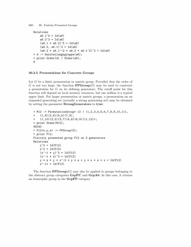
600 30. Finitely-Presented Groups
Relationsa6.1^4 = Id(a6)a6.2^3 = Id(a6)(a6.1 * a6.2)^5 = Id(a6)(a6.2, a6.1)^2 = Id(a6)(a6.2 * a6.1^-2 * a6.2 * a6.1^2)^2 = Id(a6)
> d := Darstellungsgruppe(a6);> print Order(d) / Order(a6);6
30.2.5 Presentations for Concrete Groups
Let G be a finite permutation or matrix group. Provided that the order ofG is not too large, the function FPGroup(G) may be used to constructa presentation for G on its defining generators. The cutoff point for thisfunction will depend on local memory resources, but one million is a typicalupper limit. For larger permutation or matrix groups, a presentation on anexpanded generating set (actually a strong generating set) may be obtainedby setting the parameter StrongGenerators to true:
> M12 := PermutationGroup< 12 | (1,2,3,4,5,6,7,8,9,10,11),> (1,9)(2,6)(4,5)(7,8),> (1,10)(2,5)(3,7)(4,8)(6,9)(11,12)>;> print Order(M12);95040> F12<x,y,z> := FPGroup(G);> print F12;Finitely presented group F12 on 3 generatorsRelations
y^2 = Id(F12)z^2 = Id(F12)(x^-1 * y)^3 = Id(F12)(x^-1 * z)^3 = Id(F12)y * z * y * x^-2 * y * z * y * x * z * x = Id(F12)x^-11 = Id(F12)
The function FPGroup(G) may also be applied to groups belonging tothe abstract group categories GrpPC and GrpAb. In this case, it returnsan isomorphic group in the GrpFP category.

30.3 Special Quotients 601
Table 30.3. Finitely-presented group information
Magma Meaning
Generators(G) Set containing the defining generators for G
Ngens(G) Number of defining generators for G
Relations(G) Sequence containing the defining relations forG
GeneratingWords(G, H) Given a subgroup H of group G, return gen-erators for H as words in the generators of G(if known)
30.2.6 Access Functions for Finitely Presented Groups
Table 30.3 summarizes the basic access functions which are particular tofinitely-presented groups.
30.3 Special Quotients
Considerable progress towards an understanding of the structure of an fp-group may often be achieved through the examination of various kinds ofquotients. Very effective algorithms exist for computing abelian, p-group andnilpotent quotients. Progress has also been made towards computing solublequotients of moderate size.
30.3.1 Abelian Quotients
Usually the first step in investigating a group defined by a presentation is tolook at its abelian quotients. Magma provides two functions for this purpose.The function AbelianQuotient(G) constructs the derived quotient groupG/G′ of G, i.e., the largest abelian quotient of G. The quotient is constructedas a magma in the category of abelian groups, GrpAb. The function returnsthe natural surjection φ : G → A as a second return value. Alternatively, thefunction AbelianQuotientInvariants(G) returns the invariant factors andtorsion-free rank of G/G′ in the form of a sequence. The first r terms of thesequence contain the invariant factors [d1, . . . , dr, where di|di+1 for all i < r,while a further s zeros give the torsion-free rank. Thus, each of the s zerosrepresents an infinite cyclic factor.
As a simple example, consider the presentation
〈x, y, z, t | (xyz)6, t2 = (xz)2, (xy3zt2)2, (yt2)2 = x2z3, (xyz)4(yt)2〉

602 30. Finitely-Presented Groups
as discussed in [Joh90], p. 75:
> G<x,y,z,t> := Group< x,y,z,t | (x*y*z)^6, t^2 = (x*z)^2,> (x*y^3*z*t^2)^2, (y*t^2)^2 = x^2*z^3,> (x*y*z)^4*(y*t)^2 >;> A := AbelianQuotient(G);> print A;Abelian Group isomorphic to Z/2 + Z/6 + ZDefined on 3 generatorsRelations:
2*A.1 = 06*A.2 = 0
It can be seen that the abelian quotient of G is isomorphic to the infiniteabelian group Z/2Z ⊕ Z/6Z ⊕ Z. Therefore G itself is infinite.
As a slightly more sophisticated example consider the problem of findingthe structure of the Fibonacci group F (2, 7):
To perform this example online, type load "I96c30e1";
> F27<a, b> := Group<a, b |> a^2 * b^-2 * a^-1 * b^-2 * (a^-1 * b^-1)^2,> a * b * a * b^2 * a * b * a * b^-1 * (a * b^2)^2>;> print AbelianQuotientInvariants(F27);[ 29 ]
The output shows that the quotient is cyclic, of order 29. The next step is toinvestigate the index of obvious subgroups:
> print Index(F27, sub< F27 | a >);1
Consequently, F27 is generated by a (or b) and so must be cyclic. Hence, F27must be cyclic of order 29. This is the procedure followed by George Havaswhen he first determined the order of F27 .
30.3.2 p-Quotients
The lower p-central series of a group G is the chain of normal subgroups
Φ1(G) ¤ Φ2(G) ¤ Φ3(G) ¤ . . . ,
where

30.3 Special Quotients 603
Φ1(G) = G, Φi+1(G) = [G, Φi(G)]Φi(G)p
for i ≥ 1. The p-quotient algorithm constructs quotients of G with respect tosuccessive terms of this series. If G has a finite p-quotient then, providing thatits size does not exceed available resources, this quotient may be constructedusing the p-quotient algorithm.
Given an fp-group G, a prime p and a non-negative integer c, the functionpQuotient(G, p, c) returns two values: the largest p-quotient P of G havinglower exponent-p class at most min(c, 63), as a polycyclic group (categoryGrpPC); and the natural surjection φ : G → P . The parameter Print maybe used to provide information about the progress of the algorithm; its defaultvalue of 0 specifies no output, and the values 1–3 specify progressively moredetailed output.
The relevant primes for pQuotient may be discovered by examining theabelian quotient of G. For example, consider the Fibonacci groups F (9). Fromthe structure of its abelian quotient, F (9) has nontrivial p-quotients for p = 2and p = 19:
> F9< x1,x2,x3,x4,x5,x6,x7,x8,x9 > :=> Group< x1, x2, x3, x4, x5, x6, x7, x8, x9 |> x1*x2=x3, x2*x3=x4, x3*x4=x5, x4*x5=x6, x5*x6=x7,> x6*x7=x8, x7*x8=x9, x8*x9=x1, x9*x1=x2 >;> A := AbelianQuotient(F9);> print A;Abelian Group isomorphic to Z/2 + Z/38Defined on 2 generatorsRelations:
2*A.1 = 038*A.2 = 0
> p2 := pQuotient(F9, 2, 10 : Print := 1);Lower exponent-2 central series for F9Group: F9 to lower exponent-2 central class 1 has order 2^2Group: F9 to lower exponent-2 central class 2 has order 2^3Group completed. Lower exponent-2 central class = 2,Order = 2^3
> p19 := pQuotient(F9, 19, 10 : Print := 1);Lower exponent-19 central series for F9Group: F9 to lower exponent-19 central class 1 has order 19^1Group completed. Lower exponent-19 central class = 1,Order = 19^1

604 30. Finitely-Presented Groups
Hence the largest 2-quotient of F (9) has order 8 and the largest 19-quotienthas order 19. Consequently, the maximal nilpotent quotient has order 152.
The following example constructs the largest 2-quotient of class 4 for thegroup 〈a, b | [b, a, a], (aba)4〉:
> pQ := pQuotient(Group<a, b | (b,a,a), (a*b*a)^4>, 2, 4:> Print := 1);Lower exponent-2 central series for $Group: $ to lower exponent-2 central class 1 has order 2^2Group: $ to lower exponent-2 central class 2 has order 2^5Group: $ to lower exponent-2 central class 3 has order 2^8Group: $ to lower exponent-2 central class 4 has order 2^11
> print pQ;GrpPC : pQ of order 2048 = 2^11PC-Relations:
pQ.1^2 = pQ.4,pQ.2^2 = pQ.5,pQ.3^2 = pQ.7 * pQ.10,pQ.4^2 = pQ.8,pQ.5^2 = pQ.10 * pQ.11,pQ.6^2 = pQ.10,pQ.7^2 = pQ.10,pQ.8^2 = pQ.11,pQ.2^pQ.1 = pQ.2 * pQ.3,pQ.3^pQ.2 = pQ.3 * pQ.6,pQ.4^pQ.2 = pQ.4 * pQ.7,pQ.5^pQ.1 = pQ.5 * pQ.6 * pQ.7 * pQ.10,pQ.5^pQ.3 = pQ.5 * pQ.9 * pQ.10,pQ.6^pQ.2 = pQ.6 * pQ.9,pQ.7^pQ.2 = pQ.7 * pQ.10,pQ.8^pQ.2 = pQ.8 * pQ.10
An exponent law may be imposed on the group to which pQuotient isapplied by means of the Exponent parameter. If this is set to a positiveinteger value m, rather than its default value of 0, then the exponent lawxm = 1 will be enforced. This is demonstrated below by showing that theorder of the largest finite 4-generator group having exponent 4 is 2422:
> F4 := FreeGroup(4);> B44 := pQuotient( F4, 2, 10: Exponent := 4, Print := 1);Lower exponent-2 central series for F4Group: F4 to lower exponent-2 central class 1 has order 2^4Group: F4 to lower exponent-2 central class 2 has order 2^14Group: F4 to lower exponent-2 central class 3 has order 2^34

30.4 Subgroups 605
Group: F4 to lower exponent-2 central class 4 has order 2^89Group: F4 to lower exponent-2 central class 5 has order 2^188Group: F4 to lower exponent-2 central class 6 has order 2^272Group: F4 to lower exponent-2 central class 7 has order 2^352Group: F4 to lower exponent-2 central class 8 has order 2^392Group: F4 to lower exponent-2 central class 9 has order 2^412Group: F4 to lower exponent-2 central class 10 has order 2^422Group completed. Lower exponent-2 central class = 10, Order = 2^422
There is also a process version of the p-quotient algorithm, which allowsthe user to control the individual steps closely. Details may be found in theHandbook.
30.3.3 Other Quotients
A soluble quotient algorithm developed by Alice Niemeyer is also available, asexplained in the Handbook. However, before the algorithm can be applied, theuser must determine the orders of the terms in a certain series. The nilpotentquotient algorithm developed by Werner Nickel will be installed during 1997.This algorithm is capable of handling infinite quotients.
30.4 Subgroups
30.4.1 The sub-constructor
A subgroup H of an fp-group G may be defined either by giving a set ofgenerating words or by prescribing the action of G on the right cosets ofH. The sub-constructor is used in the usual manner to define H in termsof generators (see Chapter 4). The action of G on the cosets of H givesrise to a homomorphism φ : G → Sym(n), where n = [G : H]. Hence, asubgroup defined by such an action is created using the sub-constructor withφ appearing on the right side of the constructor (in place of the generators).
This version of sub-constructor is illustrated using the braid group B4.
> B4<x,y,z> := Braid(4);> P := PermutationGroup< 4 | (1,2), (2,3), (3,4) >;> phi := hom< B4 -> P | [ P.i : i in [1..3] ] >;> H4 := sub< B4 | phi >;> H4;Finitely presented group H4Index in group B4 is 4 = 2^2Subgroup of group B4 defined by coset table
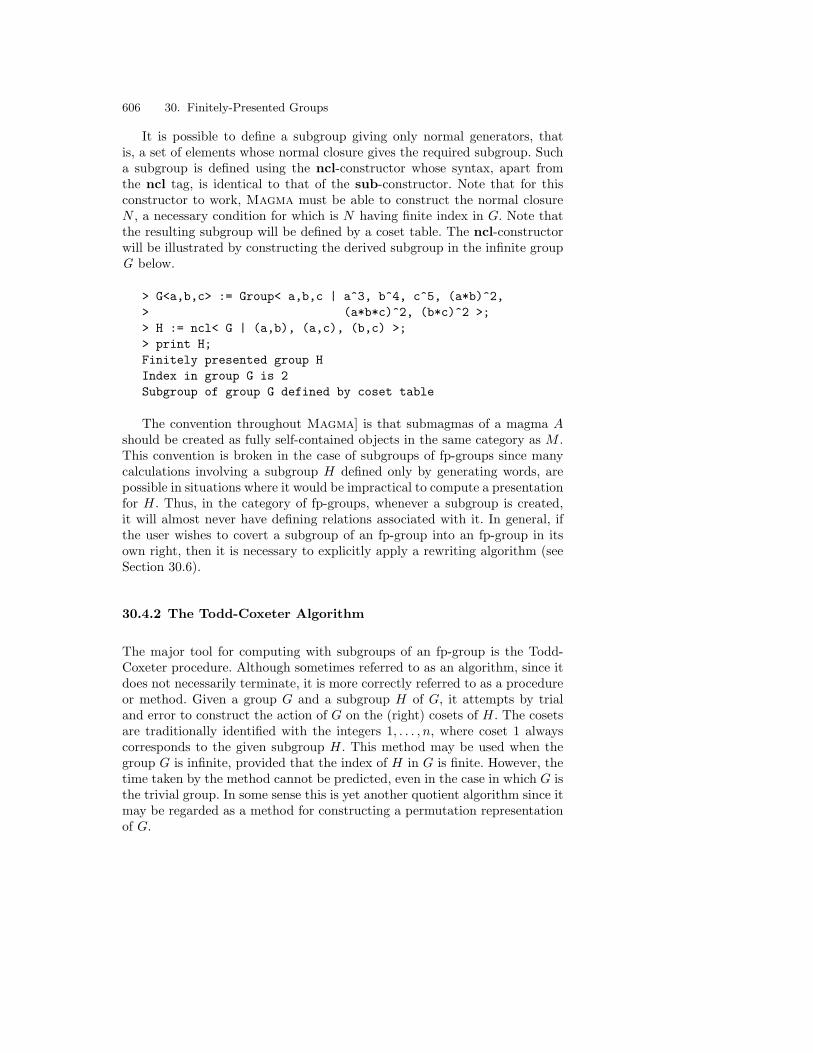
606 30. Finitely-Presented Groups
It is possible to define a subgroup giving only normal generators, thatis, a set of elements whose normal closure gives the required subgroup. Sucha subgroup is defined using the ncl-constructor whose syntax, apart fromthe ncl tag, is identical to that of the sub-constructor. Note that for thisconstructor to work, Magma must be able to construct the normal closureN , a necessary condition for which is N having finite index in G. Note thatthe resulting subgroup will be defined by a coset table. The ncl-constructorwill be illustrated by constructing the derived subgroup in the infinite groupG below.
> G<a,b,c> := Group< a,b,c | a^3, b^4, c^5, (a*b)^2,> (a*b*c)^2, (b*c)^2 >;> H := ncl< G | (a,b), (a,c), (b,c) >;> print H;Finitely presented group HIndex in group G is 2Subgroup of group G defined by coset table
The convention throughout Magma] is that submagmas of a magma Ashould be created as fully self-contained objects in the same category as M .This convention is broken in the case of subgroups of fp-groups since manycalculations involving a subgroup H defined only by generating words, arepossible in situations where it would be impractical to compute a presentationfor H. Thus, in the category of fp-groups, whenever a subgroup is created,it will almost never have defining relations associated with it. In general, ifthe user wishes to covert a subgroup of an fp-group into an fp-group in itsown right, then it is necessary to explicitly apply a rewriting algorithm (seeSection 30.6).
30.4.2 The Todd-Coxeter Algorithm
The major tool for computing with subgroups of an fp-group is the Todd-Coxeter procedure. Although sometimes referred to as an algorithm, since itdoes not necessarily terminate, it is more correctly referred to as a procedureor method. Given a group G and a subgroup H of G, it attempts by trialand error to construct the action of G on the (right) cosets of H. The cosetsare traditionally identified with the integers 1, . . . , n, where coset 1 alwayscorresponds to the given subgroup H. This method may be used when thegroup G is infinite, provided that the index of H in G is finite. However, thetime taken by the method cannot be predicted, even in the case in which G isthe trivial group. In some sense this is yet another quotient algorithm since itmay be regarded as a method for constructing a permutation representationof G.

30.4 Subgroups 607
The output of the procedure is a mapping giving the action of G on the(right) cosets of the subgroup H. Magma follows customary terminology inreferring to this mapping as the coset table for H in G. As a by-product, ifthe Todd-Coxeter terminates, it gives the index of H in G.
A number of functions directly invoke the Todd-Coxeter procedure anddiffer mainly in the information returned. These functions include ToddCoxeter,Index, CosetSpace and CosetAction. In this section, the discussion willfocus on ToddCoxeter and Index. Both of these functions take the samearguments and parameters, and return the index of H in G, or 0 if the enumer-ation fails to complete. The function ToddCoxeter returns three additionalvalues: the coset table, the maximum number of cosets, and the total numberof cosets. Several parameters allow the user to control aspects of the cosetenumeration as will be explained below.
For example, the following code enumerates the cosets of the subgroupH8723 = 〈a2, a−1b〉 in G8723 = 〈a, b | a8, b7, (ab)2, (a−1b)3〉:
To perform this example online, type load "I96c30e2";
> G8723<a, b> := Group< a, b |> a^8, b^7, (a * b)^2, (a^-1 * b)^3 >;> H8723 := sub< G8723 | a^2, a^-1 * b >;> print Index(G8723, H8723);448
From the output, the number of cosets of H8723 in G8723 is 448.
A zero value returned by a function invoking the Todd-Coxeter methodindicates that the enumeration has failed to complete using a given amountof memory.No mathematical conclusion can be drawn from this outcome. Itcannot be concluded that the index is infinite, though this may well be thecase. In these circumstances, different parameter values (see below) or moresophisticated techniques are required to settle the issue. It is most importantto note that the default limit on the memory limit for coset enumeration isquite small and that for all serious or hard enumerations, the user will needto explicitly set his/her own limit as described below.
A large number of different strategies may be employed by the Todd-Coxeter method. The default strategy may be unsuitable for many particularenumerations, in that the method may exhaust the resources before com-pleting. It is therefore necessary for the user to become familiar with someof the parameters which manipulate the progress of the function. The mostimportant of these is CosetLimit, which gives an upper limit on the num-ber of cosets that may be defined at any stage of the process. (In the caseof hard enumerations, it is frequently true that the method will introduce a

608 30. Finitely-Presented Groups
substantially larger number of cosets than the index of H in G.) By default,CosetLimit is approximately one million divided by the number of gener-ators. However, when enumerating the cosets of a subgroup of large index,or when attempting to perform a hard enumeration, it may be necessary toincrease this value. Alternatively, in other circumstances it may be desirableto lower this limit.
The example below illustrates the effect of CosetLimit. It will be seenthat for the groups G8723 and H8723 , the enumeration fails when the pa-rameter is set to 1000 or 2000, but succeeds for 3000:
> index := ToddCoxeter(G8723, H8723: CosetLimit := 1000);> print index;0> index := ToddCoxeter(G8723, H8723: CosetLimit := 2000);> print index;0> index := ToddCoxeter(G8723, H8723: CosetLimit := 3000);> print index;448
Another important parameter is Print, which controls the level of infor-mative printing during the execution of the function. It takes a small non-negative integer as its value (default 0). The value 0 indicates no printing;the value 1 merely causes statistics to be printed upon termination; the value2 produces a message giving the current maximum and the total cosets tobe printed after every m cosets, where the frequency m may be set usingthe Grain parameter (default 10 000). Observation of trends in these valuesfrequently indicates whether or not the enumeration is likely to complete.For example, the following (slightly edited) output indicates the informationprinted when Print is set to 2 and Grain is set to 500:
> G8723<a, b> := Group< a, b |> a^8, b^7, (a * b)^2, (a^-1 * b)^3 >;> H8723 := sub< G8723 | a^2, a^-1 * b >;> index := ToddCoxeter(G8723, H8723: Print := 2,> Grain := 500);Maximum table size = 499829
Fill Factor = 7, CT Factor = 0, RT Factor = 0RD alive= 500, Max= 500, Total= 547RD alive= 1000, Max= 1000, Total= 1142RD alive= 1500, Max= 1500, Total= 1745RD alive= 2000, Max= 2000, Total= 2417RC alive= 1500, Max= 2176, Total= 2626RC alive= 1000, Max= 2176, Total= 2626
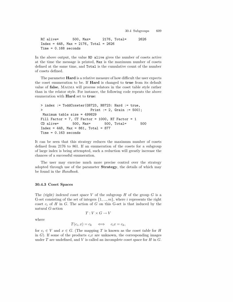
30.4 Subgroups 609
RC alive= 500, Max= 2176, Total= 2626Index = 448, Max = 2176, Total = 2626Time = 0.168 seconds
In the above output, the value RD alive gives the number of cosets activeat the time the message is printed, Max is the maximum number of cosetsdefined at the same time, and Total is the cumulative count of the numberof cosets defined.
The parameter Hard is a relative measure of how difficult the user expectsthe coset enumeration to be. If Hard is changed to true from its defaultvalue of false, Magma will process relators in the coset table style ratherthan in the relator style. For instance, the following code repeats the aboveenumeration with Hard set to true:
> index := ToddCoxeter(G8723, H8723: Hard := true,> Print := 2, Grain := 500);Maximum table size = 499829
Fill Factor = 7, CT Factor = 1000, RT Factor = 1CD alive= 500, Max= 500, Total= 500Index = 448, Max = 861, Total = 877Time = 0.163 seconds
It can be seen that this strategy reduces the maximum number of cosetsdefined from 2176 to 861. If an enumeration of the cosets for a subgroupof large index is being attempted, such a reduction will greatly increase thechances of a successful enumeration.
The user may exercise much more precise control over the strategyadopted through use of the parameter Strategy, the details of which maybe found in the Handbook.
30.4.3 Coset Spaces
The (right) indexed coset space V of the subgroup H of the group G is aG-set consisting of the set of integers 1, ...,m, where i represents the rightcoset ci of H in G. The action of G on this G-set is that induced by thenatural G-action
T : V ×G → V
whereT (ci, x) = ck ⇐⇒ cix = ck,
for ci ∈ V and x ∈ G. (The mapping T is known as the coset table for Hin G). If some of the products cix are unknown, the corresponding imagesunder T are undefined, and V is called an incomplete coset space for H in G.

610 30. Finitely-Presented Groups
The Todd-Coxeter method may be viewed as constructing a coset space.While the Index and ToddCoxeter functions emphasize the determinationof the index of a subgroup H in the group G, the actual coset space is ofinterest in a number of situations. For example, if the Todd-Coxeter methodfails to terminate, an incomplete coset space may be used to build a sub-group that properly contains H. Iterating the process a number of times mayresult in constructing a subgroup for which the Todd-Coxeter does termi-nate. Again, the complete coset space yields a permutation representationfor G. The function for constructing a coset space (complete or incomplete)is CosetSpace(G,H). It has the same parameters as ToddCoxeter, andthe user will often need to over-ride the default values. Some elementaryfunctions for coset spaces are given in Table 30.4. Further operations may befound in Table 30.7.
Table 30.4. Operations on Coset Spaces
Magma Meaning
#V Cardinality of the coset space V
Action(V ) Mapping (coset table) T : V ×G → V giving theaction of G on the coset space V
T (i, w) Image of coset i and word w with respect to thecoset action mapping T
IsComplete(V ) Returns true if V is a complete coset space
ExcludedConjugates(V ) Conjugates of the generators of subgroup H bythe generators of G that lie outside of H, accord-ing to the (complete or incomplete) coset spaceV of H in G
ExcludedConjugates(T ) As above, but according to the (complete or in-complete) coset table T of H in G
The following example illustrates the use of coset spaces in building sub-groups. It gives a function DerSubgroup which computes the derived subgroupG′ for the fp-group G (assuming that the Todd-Coxeter method can constructthe coset space of G′ in G):
DerSubgroup := function(G)/* Initially define S to contain the commutator
of each pair of generators of G */S := commut : x, y in Generators(G) |
commut ne Id(G) where commut is (x,y) ;/* Successively extend S until it is closed under
conjugation by the generators of G */repeat
V := CosetSpace(G, sub<G | S>);

30.4 Subgroups 611
E := ExcludedConjugates(V);S := S join E;
until #E eq 0;return sub<G | S>;
end function;
The function is now used to construct the derived subgroup of the infinite2-dimensional crystallographic group 〈a, b | a3, b2, (a ∗ b)6〉:
> G<a, b> := Group< a, b | a^3, b^2, (a*b)^6 >;> D := DerSubgroup(G);> print D;Finitely presented group D on 6 generatorsIndex in group G is 6 = 2 * 3Generators as words in group G
D.1 = (a^-1, b)D.2 = (a, b)D.3 = (b, a^-1)D.4 = a^-2 * b^-1 * a * b * aD.5 = a^-1 * b^-1 * a^-1 * b * a^2D.6 = (b, a)
30.4.4 Subgroup Constructions
Table 30.5. Operations on Subgroups
Magma Meaning
H^x Conjugate of subgroup H by element x
H meet K Intersection of H and K
Core(G, H) Largest normal subgroup of G contained in H
MaximalOvergroup(G, H) Maximal subgroup of G containing H
MinimalOvergroup(G, H) Subgroup of G which contains H as a maximalsubgroup
Normalizer(G, H) Normalizer of H in G
NormalClosure(G, H) Normal closure of H in G
SchreierGenerators(G, H) Schreier generators for H in G
SchreierSystem(G, H) System of coset representatives for H in G
Transversal(G, H, K) System of representatives for the double cosetsHuK for the subgroups H and K of G
Let H and K be subgroups of the fp-group G. It is possible to computevarious subgroups relating to H and K knowing only a set of generating

612 30. Finitely-Presented Groups
Table 30.6. Boolean Operations on Subgroups
H eq K u in H H subset K
IsConjugate(G, H, K) IsNormal(G, H) IsMaximal(G, H)
words and a coset table for H in G. The major operations that return asubgroup are summarized in Table 30.5, and some boolean operations arelisted in Table 30.6.
The example below applies these subgroup constructions in order to con-struct subgroups of small index in the two-dimensional space group p4g hav-ing presentation 〈r, s | r2, s4, (r, s)2〉:
> p4g<r, s> := Group< r, s |> r^2 = s^4 = (r, s)^2 = 1 >;> print p4g;Finitely presented group p4g on 2 generatorsRelations
r^2 = Id(p4g)s^4 = Id(p4g)(r, s)^2 = Id(p4g)
> h := sub< p4g | (s^-1 * r)^4, s * r >;> k := sub< p4g | (s^-1 * r)^2, (s * r)^2 >;> print Index(p4g, h), Index(p4g, k);8 8> n := NormalClosure(p4g, h);> print n;Finitely presented group n on 5 generatorsIndex in group p4g is 2Generators as words in group p4g
n.1 = (s^-1 * r)^4n.2 = s * rn.3 = r * sn.4 = r^-1 * s * r^2n.5 = s^2 * r * s^-1
> m := MinimalOvergroup(p4g, h);> print m;Finitely presented group m on 3 generatorsIndex in group p4g is 4 = 2^2Generators as words in group p4g
m.1 = (s^-1 * r)^4m.2 = s * rm.3 = (r * s)^2
> n := MaximalOvergroup(p4g, k);

30.5 Permutation Representations 613
> print n;Finitely presented group n on 4 generatorsIndex in group p4g is 2Generators as words in group p4g
n.1 = (s^-1 * r)^2n.2 = (s * r)^2n.3 = rn.4 = s^2
> l := h meet k;> print l;Finitely presented group lIndex in group p4g is 16 = 2^4Subgroup of group p4g defined by coset table> j := h^s;> print j;Finitely presented group j on 2 generatorsIndex in group p4g is 8 = 2^3Generators as words in group p4g
j.1 = (s^-2 * r * s)^4j.2 = r * s
> print j eq h;false> print IsConjugate(p4g, h, j);true r^-1> c := Core(p4g, h);> print Index(p4g, c);32
30.5 Permutation Representations
The action of G on the coset space V of a subgroup H gives a permu-tation representation of G. This construction yields yet another type ofquotient, and may be used to discover non-soluble composition factors ofG. Such a representationa may be constructed by means of the functionCosetAction(G,H), as discussed in Section ??. However, note that thisfunction only returns the action and the image when G and H are fp-groups,since the kernel of the action is difficult to compute unless the index of thekernel in G is very small. If the user desires the kernel, it must be obtainedusing CosetKernel(G,H) or Core(G,H).
For example:
> G8723m, G8723L := CosetAction(G8723, H8723);

614 30. Finitely-Presented Groups
> print G8723L, G8723m;Permutation group G8723L of degree 448Mapping from: GrpFP: G8723 to GrpPerm: G8723L
For more difficult examples, CosetAction(G,H) may not be sufficientto construct a permutation representation of G. In this case, the coset spaceV should be constructed with a parametrized call to CosetSpace(G,H),and then one of the functions in Table 30.7 should be used to extract thepermutation representation.
Table 30.7. Representations Afforded by Coset Spaces
Magma Meaning
CosetAction(V ) Returns (i) homomorphism of G into a permutationgroup L given by the action of G on the coset space Vof H; (ii) image L
CosetAction(G, H) Returns (i) homomorphism of G into a permutationgroup L given by the action of G on the coset space ofH; (ii) image L
CosetImage(V ) Image of CosetAction(V )
CosetImage(G, H) Image of CosetAction(G, H)
CosetKernel(V ) Kernel of CosetAction(V ) (only practical when [G :H] is small)
CosetKernel(G, H) Kernel of CosetAction(G, H) (only practical when[G : H] is small)
The difficult step in constructing a permutation representation is findinga suitable subgroup. This will sometimes be known from the manner in whichthe presentation has been constructed. Another approach is to examine sub-groups generated by random words in the hope of finding one with the desiredproperties. In the final section in this chapter, a systematic method is givenfor locating all subgroups having index less than or equal to some modestlimit.
The following code constructs a permutation representation of degree1140 000 for the Harada-Norton simple group. A subgroup H having thisindex is known from the manner in which the presentation was constructed.Because the index of H is so large, the function CosetAction would fail,since it would invoke the Todd-Coxeter method with default values for theparameters:
> HN<x, a, b, c, d, e, f, g > :=> Group< x, a, b, c, d, e, f, g |> x^2, a^2, b^2, c^2, d^2, e^2, f^2, g^2,

30.6 Presentations for Subgroups 615
> (x, a), (x, g),> (b*c)^3, (b*d)^2, (b*e)^2, (b*f)^2, (b*g)^2,> (c*d)^3, (c*e)^2, (c*f)^2, (c*g)^2,> (d*e)^3, (d*f)^2, (d*g)^2,> (e*f)^3, (e*g)^2,> (f*g)^3,> (b, x*b*x),> (a, e*d*c*b), (a, f)*d*c*b*d*c*d, (a*g)^5,> (c*d*e*f, x*b*x), (b, x*c*d*e*f*x),> (c*d*e*f, x*c*d*e*f*x) >;> H := sub< HN | x,b,c,d,e,f,g>;> cstspc := CosetSpace(HN, H: CosetLimit := 1200000,> Hard := true, Print := 1);Fill Factor = 12, CT Factor = 1000, RT Factor = 1Index = 1140000, Max = 1141309, Total = 1470174Time = 132.900 seconds
> G := CosetImage(cstspc);> print G;Permutation group G acting on a set of cardinality 1140000> print Order(G);546061824000000> print FactoredOrder(G);[ <2, 15>, <3, 6>, <5, 6>, <7, 1>, <11, 1>, <19, 1> ]> time print CompositionFactors(G);
G| Cyclic(2)*| HA1
Time: 3941.309
30.6 Presentations for Subgroups
Suppose that G is a fp-group whose defining presentation has r generatorsand s relations. Let H be some subgroup of G having finite index n whichhas been created by Magma. However H was constructed, it will be initiallydefined either in terms of a set of generating words or in terms of the actionof G on its cosets (i.e. by means of a coset table). For some applications,it will be necessary to have H as a fp-group and this means constructing apresentation for it. Such a presentation may be obtained by rewriting therelations stored for G using the Reidemeister-Schreier algorithm. Unfortu-nately, the Reidemeister-Schreier algorithm constructs a presentation involv-

616 30. Finitely-Presented Groups
ing (n − 1)r + 1 generators and n ∗ s relations. Clever techniques based onthe use of Tietze transformations have been developed to simplify such pre-sentations. Even so, the use of subgroup rewriting is restricted to subgroupsof modest index.
The function Rewrite(G,H) returns an fp-group K isomorphic to H andembedded in G. Note that the default rewriting procedure will not, in gen-eral, construct the presentation on the original generators for H. By default,Rewrite automatically performs simplification on the rewritten presenta-tion, but the user may turn it off by setting the parameter Simplify to false.It should be noted that the simplification procedure will often eliminate alarge number of the generators of K at the cost of producing long relations.For some applications these long relations are harmful and so controled sim-plification needs to be performed using the techniques discussed in the nextsection.
The Rewrite function will be illustrated by proving that the group〈a, b | a6, b6, ab2 = ba2〉 is infinite:
>G<a, b> := Group<a, b | a^6 = b^6 = 1, a * b^2 = b * a^2>;> print AbelianQuotientInvariants(G);[ 6 ]> H := ncl<G | (a,b)>;> print Index(G, H);6> K := Rewrite(G, H);> print K;Finitely presented group K on 2 generatorsGenerators as words in group G
K.1 = b * a^-1K.2 = a * b * a^-2
RelationsK.1^2 * K.2 * K.1^2 * K.2^-1 = Id(K)K.1 * K.2^2 * K.1^-1 * K.2^2 = Id(K)
> print AbelianQuotientInvariants(K);[4, 4]> L := ncl<K | (K.1, K.2)>;> print Index(K, L);16> M := Rewrite(K, L);> print M;Finitely presented group M on 3 generatorsGenerators as words in group K
M.1 = (K.1, K.2^-1)M.2 = (K.2^-1, K.1^-1)M.3 = (K.2, K.1^-1)

30.6 Presentations for Subgroups 617
Relations(M.1^-1, M.2^-1) = Id(M)(M.1^-1, M.3^-1) = Id(M)(M.2^-1, M.3^-1) = Id(M)
> print AbelianQuotientInvariants(M);[ 0, 0, 0 ]
The subgroup M has index 96 in G and its abelian quotient is infinite. Itfollows that G is infinite.
The next example constructs a presentation for a subgroup defined by acoset table. The braid group Bn, considered in Section 30.2.2, has a subgroupHn of index n which is constructed as follows. As noted in Section 30.2.2 thereis a homomorphism φ : Bn → Sn, where Sn is isomorphic to Sym(n). Thesubgroup Hn of Bn is the preimage of the stabilizer of 1 in Sym(n) withrespect to the homomorphism τ : Bn → Sym(n).
> B4<x,y,z> := Braid(4);> S4<a,b,c>, phi := quo< B4 | x^2 = y^2 = z^2 = 1 >;> rho := CosetAction(S4, sub< S4 | b, c >);> H4 := sub< B4 | phi*rho >;> H4<l,m,n> := Rewrite(B4, H4);> print H4;Finitely presented group H4 on 3 generatorsGenerators as words in group B4
l = ym = zn = x^2
Relationsl * n * l * n^-1 * l^-1 * n^-1 = Id(H4)n^-1 * l * m * l^-1 * n * l * m^-1 * l^-1 = Id(H4)l * n^-1 * m * n * l^-1 * n^-1 * m^-1 * n = Id(H4)m^-1 * l^-1 * m^-1 * l * m * l * m * l^-1 = Id(H4)m^-1 * n^-1 * m^-1 * n * m * n * m * n^-1 = Id(H4)
The subgroup Hn plays a key role in the study of braid groups. It is a semidi-rect product of the free group of rank n− 1 with the braid group Bn−1. (See[Joh90]).
An important special case of subgroup rewriting occurs when the objec-tive is to use the presentation of the subgroup H of the fp-group G in orderto determine the structure of the derived quotient group, H/H ′. Rather thanproducing all the relations of H at once and then abelianizing, the functionAbelianQuotient(G, H) abelianizes each relator as it is produced, therebypossibly saving a large amount of time and memory. Similarly, the func-tion AbelianQuotientInvariants(G,H) returns the invariant factors and

618 30. Finitely-Presented Groups
torsion-free rank of H/H ′. These versions of the functions are frequently use-ful when attempting to prove that G is infinite. Even when G has a finiteabelian quotient, it may have subgroups of small index possessing infiniteabelian quotients. For example:
> G<x,z> := Group< x, z | z^3*x*z^3*x^-1, z^5*x^2*z^2*x^2 >;> H := sub< G | x, z*x*z, z*x^-1*z*x*z^-1>;> print AbelianQuotientInvariants(H);[ 2, 6, 0 ]
The zero at the end of the sequence of invariants indicates that the abelianquotient has an infinite summand.
30.7 Simplifying a Presentation
It frequently happens that a presentation contains redundant generatorsand/or relations. This is usually the case if the presentation has been con-structed by means of some rewriting method such as the Reidemeister-Schreier algorithm. The function Simplify(G) attempts to eliminate gen-erators and to shorten relators by locating substrings that correspond to theleft or right hand side of a relation. It returns a new group K, isomorphic toG, whose defining presentation is the simplified presentation for G.
For example, the Fibonacci group F (n) is generated by the set x1, . . . , xnwith the defining relations xixi+1 = xi+2, for i ∈ 1, . . . , n, where the sub-scripts are taken modulo n. It is easily seen that any Fibonacci group F (n)can be given as a 2-generator group. The code below invokes Simplify toobtain the 2-generator presentation for F (7):
> F7<x1,x2,x3,x4,x5,x6,x7> := Group< x1,x2,x3,x4,x5,x6,x7 |> x1*x2=x3, x2*x3=x4, x3*x4=x5, x4*x5=x6,> x5*x6=x7, x6*x7=x1, x7*x1=x2 >;> K<a,b> := Simplify(F7);> print K;Finitely presented group K on 2 generatorsRelations
a^2 * b^-1 * a * b^-1 * a * b^2 * a * b = Id(K)a^2 * b^-1 * a^2 * b^-1 * a * b^-2 * a^-1 * b^-1 = Id(K)
The Simplify function has a parameter Iterations which allows theuser to bound the number of times the main elimination loop is executed.(By default, there is no limit.) Usually, one generator is eliminated for eachiteration of the loop. There is also a process version, allowing the user to

30.8 Locating Subgroups of Finite Index 619
direct the simplification algorithm. The reader is referred to the Handbookfor details.
30.8 Locating Subgroups of Finite Index
It is frequently desirable to know all subgroups of an fp-group G whichhave index less than or equal to some given (small) bound. For instance,if it is known that G has a non-trivial subgroup, then G cannot be trivial.Magma provides two related functions for constructing subgroups of lowindex: LowIndexSubgroups simply returns a sequence of subgroups; andLowIndexProcess constructs a process from which the user may extract asmany low index subgroups as desired.
30.8.1 Subgroups of Low Index
The functions LowIndexSubgroups(G,R) returns a sequence of subgroupsof the group G satisfying certain bound conditions described by R. The ar-gument R may either be an integer, giving an upper bound on the index, ora 2-tuple of integers, giving a lower bound and an upper bound. The termsof the sequence are arranged in non-decreasing order of the subgroup index,and each entry of the sequence is a representative for a distinct conjugacyclass of subgroups.
For example, suppose the user wishes to calculate all conjugacy classesof subgroups of the infinite triangle group 〈x, y | x2, y2, (xy)7〉 having indexless than or equal to 12. The appropriate statements are:
> G<x, y> := Group<x, y | x^2, y^3, (x*y)^7 >;> L := LowIndexSubgroups(G, 12);[
Finitely presented group on 2 generatorsIndex in group G is 1Generators as words in group G
$.1 = x$.2 = y,
Finitely presented group on 3 generatorsIndex in group G is 7Generators as words in group G
$.1 = x$.2 = y * x * y^-1$.3 = y^-1 * x * y^-1 * x * y * x * y,

620 30. Finitely-Presented Groups
Finitely presented group on 3 generatorsIndex in group G is 7Generators as words in group G
$.1 = x$.2 = y * x * y^-1$.3 = y^-1 * x * y * x * y^-1 * x * y,
Finitely presented group on 2 generatorsIndex in group G is 8 = 2^3Generators as words in group G
$.1 = y$.2 = x * y * x * y * x * y^-1 * x,
Finitely presented group on 2 generatorsIndex in group G is 9 = 3^2Generators as words in group G
$.1 = x$.2 = y * x * y * x * y * x * y^-1
]
If the user wishes to impose a lower bound l as well as an upper bound u onthe size of the index, then R should be given in the form of a tuple < l, u >.For example, the following statement determines the number of conjugacyclasses of subgroups of G having index exactly 50:
> L := LowIndexSubgroups(G, <50, 50>);> print #L;333> print L[10];Finitely presented group on 4 generatorsIndex in group G is 50 = 2 * 5^2Generators as words in group G
$.1 = x$.2 = y * x * y * x * y^-1 * x * y^-1 * x * y * x
* y * x * y^-1$.3 = y^-1 * x * y * x * y^-1 * x * y * x * y^-1
* x * y^-1 * x * y * x * y$.4 = y * x * y * x * y * x * y^-1 * x * y^-1 * x
* y * x * y * x * y^-1 * x * y * x * y
LowIndexSubgroups has several parameters. The most important ofthem are Limit, Subgroup, and Print. If the user assigns a positive integerto Limit, the function will terminate after finding n conjugacy classes in thegiven index range. Otherwise, there is no theoretical limit to the number of

30.8 Locating Subgroups of Finite Index 621
classes Magma finds. If a subgroup H of G is assigned to the parameterSubgroup, Magma will restrict its search for subgroups of appropriate in-dex to those subgroup classes in which at least one subgroup contains H.The default value of Subgroup is the trivial subgroup, so that the functionnormally returns all the subgroups in the index range.
The Print parameter allows the user to control the amount of output thatMagma gives when LowIndexSubgroups is invoked. By default (value 0),no intermediate printing is given. If Print is assigned 1, 2, or 3, Magmagives output progressively as it calculates the low index subgroups. For thevalue 1, Magma prints for each class the index, the length, and a set ofgenerators for the class representative. For the value 2, it also prints the per-mutation representation of G on the right cosets of the class representative,and for the value 3 it also prints generators for the normalizer N of the classrepresentative and a system of right coset representatives for N in G.
As an illustration of the use of these parameters, consider the problemof finding five subgroups of G which contain H8723 . Certainly if a subgroupcontains H8723 its index cannot exceed the index of H8723 , and so 448, theindex of H8723 , will do well for an upper bound. The following line showshow to calculate the subgroups, requesting a maximum of 5 subgroups bymeans of the Limit parameter, and obtaining a small amount of outputimmediately after each class is constructed:
> LH8723 := LowIndexSubgroups(G8723, 448: Print := 1,> Limit := 5, Subgroup := H8723);Subgroup class 1 Index 7 Length 7Subgroup generators :- a^2, a^-1 * b, b * a^-1 * b^-2
Subgroup class 2 Index 7 Length 7Subgroup generators :- a^2, a * b^-2 * a^-1 * b * a^-1, a^-1 * b
Subgroup class 3 Index 14 Length 7Subgroup generators :- a^2, b^2 * a^-2 * b * a^-1, a^-1 * b
Subgroup class 4 Index 14 Length 7Subgroup generators :- a^2, (b^2 * a^-1 * b^-2)^2, a^-1 * b
Subgroup class 5 Index 28 Length 28Subgroup generators :- (b^3 * a^-1 * b^-3)^4, a^2, b * a^-3 * b * a^-1,b^2 * a^2 * b * a^-1 * b^-2 * a^-2 * b^-2,

622 30. Finitely-Presented Groups
(b^2 * a^-1 * b^-2)^4, a^-1 * b
> print foralls:s in LH8723 |> s subset G8723 and H8723 subset s;true
30.8.2 The Low Index Subgroups Process
LowIndexProcess(G,R) operates similarly to LowIndexSubgroups, andhas the same parameters, except that after Magma calculates each subgroupclass it stops and returns control to the user, allowing the user to decidewhether or not to find another subgroup class. The function returns a processP , not a subgroup class, and other intrinsics are used to manipulate thisprocess.
For instance, the following line creates a process for the situation describedin the example above:
> PH8723 := LowIndexProcess(G8723, 448: Subgroup := H8723);> print PH8723;Low Index Subgroups Process
The function ExtractGroup(P ) is required in order to obtain the currentconjugacy class from the process. In the statement below, the identifier nextCis assigned the new conjugacy class representative:
> nextC := ExtractGroup(PH8723); print nextC;Finitely presented group nextC on 3 generatorsIndex in group G8723 is 7Generators as words in group G8723
nextC.1 = a^2nextC.2 = a^-1 * bnextC.3 = b * a^-1 * b^-2
Notice that the low index process does not return the subgroup of index 1first; it saves it to be the last class.
The function ExtractGenerators(P ) returns the set of generators ofthis current class:
> gens := ExtractGenerators(PH8723); print gens; a^2, a^-1 * b, b * a^-1 * b^-2
ExtractGroup and ExtractGenerators only give information aboutthe current conjugacy class. If the user decides to advance along the process

30.8 Locating Subgroups of Finite Index 623
to the next class, the procedure NextSubgroup(˜P ) must be invoked. Thetilde symbol ˜ is necessary since the procedure modifies the process P :
> NextSubgroup(~PH8723);> nextC := ExtractGroup(PH8723); print nextC;Finitely presented group nextC on 3 generatorsIndex in group G8723 is 7Generators as words in group G8723
nextC.1 = a^2nextC.2 = a^-1 * bnextC.3 = a * b^-2 * a^-1 * b * a^-1
These operations should be continued until the user has found all the desiredconjugacy classes of low index subgroups.
If all of the classes are extracted, then the process becomes empty. Thefollowing example demonstrates this on a very small group:
> G3 := SymmetricGroup(GrpFP, 3);> P3 := LowIndexProcess(G3,7);> print ExtractGroup(P3);Finitely presented group on 1 generatorIndex in group G3 is 2Generators as words in group G3
$.1 = G3.1> NextSubgroup(~P3);> print ExtractGroup(P3);Finitely presented group on 1 generatorIndex in group G3 is 3Generators as words in group G3
$.1 = G3.2> NextSubgroup(~P3);> print ExtractGroup(P3);Finitely presented group on 1 generatorIndex in group G3 is 6 = 2 * 3Generators as words in group G3
$.1 = Id(G3)> NextSubgroup(~P3);> print ExtractGroup(P3);
>> print ExtractGroup(P3);^
Runtime error in ’ExtractGroup’: Argument 1 is not non-empty

624 30. Finitely-Presented Groups
To avoid this eventual error message, the user may prefer to test the pro-cess each time it is modified by means of the function IsEmpty(P ). Thisfunction returns true if there are no more classes left. IsEmpty(P ) is par-ticularly useful if the examination of the process forms part of a user-definedfunction/procedure, rather than being undertaken interactively.
30.9 Finite Groups
There are two important problems relating to finite fp-groups. The first, nat-urally, is to decide whether or not a particular fp-group G is finite. Secondly,if a group is known to be finite, it is often desirable to construct a faithfulrepresentation for it in some group category having an element normal formso that the structure of the group may be investigated in detail.
30.9.1 Determining the Order
Proving that a group is finite is often quite difficult. The function Order(G)tries to deduce the order of G by reducing the problem to enumerating cosetsof some group over its trivial subgroup. If it is unable to determine theorder, it returns zero. Order takes the same parameters as Index. The usershould be aware that by default, Order the memory allocation for the cosetenumeration is quite small and for larger or more difficult finite groups, theuser may have to reset the parameter CosetLimit to a much higher value.More likely, the user will need to adopt a more sophisticated approach.
The standard approach to this problem involves constructing “by hand”a sequence of subgroups
G ≥ H1 ≥ H2 . . . ≥ Hr,
where Hr is the trivial subgroup, and showing that each subgroup has finiteindex in its larger neighbour. In fortunate circumstances, it may be possibleto identify a subgroup of known order from the presentation defining G.Otherwise, the subgroups in the chain are constructed in various ways. Forexample, if G is not perfect, the first subgroup will usually be the kernelof a homomorphism corresponding to a quotient obtained using one of thetechniques discussed in Section 30.3.
Throughout this chapter, various groups have been shown to be infiniteby demonstrating that they possess an infinite section. Another technique forproving that a group is infinite involves trying to construct a homomorphismonto a known infinite group. Producing such a proof is very much an art andmany familiar groups such as the Fibonacci group F (2, 9) ([Joh90]) resistedattempts to establish their infinite order for many years.

30.9 Finite Groups 625
30.9.2 Constructing a Representation
If G is known to be finite, there are various approaches to constructing agroup K in a category with an element normal form, that is isomorphic toG. If G is known to be a p-group, the p-quotient algorithm may be used toconstruct a pc-group K. If G is known to be soluble, the soluble quotientalgorithm may be used in a similar manner. Otherwise, it will be necessaryto construct a permutation representation for G over a core-free subgroup. Ina future release of Magma, it will be possible to represent the multiplicationtable of G by means of a Cayley graph.


31. Abelian Groups
Abelian groups are groups in which all the elements commute with one an-other. Because of this, it is customary to write expressions within an abeliangroup additively. Magma uses a+b,−a and 0 in its implementation of abeliangroups, whereas it uses a*b, a^−1 and 1 in all other group categories.
31.1 Constructing the Free Abelian Group
The free abelian group F of rank n is the abelian group that has n gen-erators, with no relations on them. The function for creating this group isFreeAbelianGroup(n). For example:
> F4 := FreeAbelianGroup(4);> print F4;AbelianGroup isomorphic to 4 ZDefined on 4 generators (free)
The category of abelian groups is GrpAb.
The ith generator of F4 can be obtained as F4 .i. However, it is generallyeasier to give special names to the generators using the angle bracket notation:
> F4<w, x, y, z> := FreeAbelianGroup(4);
The letters w, x, y, z behave both as alternative identifier names and as print-names for the generators.
31.2 Computing with Abelian Group Elements
The identity element of an abelian group A is the additive identity. Theexpressions A!0 or Id(A) return this element, and IsId(a) tests whether theelement a is the identity element:

628 31. Abelian Groups
> print Id(F4);0> print IsId(F4!0);true
A general element or word a in an abelian group A with n generators hasthe form a = a1e1 + · · · + arer, where the ai are integers and the ei are thegenerators. There are two main ways to create a in Magma, either as anexpression in the generators, using + and * signs, or as an integer sequence[a1, . . . , an] that is coerced into A. For instance, the following statementscreate the element g = 4w − 5x + z of F4 in each way, and test that theresults are the same:
> g := 4*w - 5*x + z;> print g;4*w - 5*x + z> print F4![4,-5,0,1] eq g;true
If A has only one generator, e1, then A!a1 may be used as an alternative toA![a1]:
> print FreeAbelianGroup(1)!8;8
The function ElementToSequence(a) or Eltseq(a) returns the se-quence [a1, . . . , an] corresponding to the element a = a1e1 + · · ·+ arer:
> print ElementToSequence(g);[ 4, -5, 0, 1 ]
Addition is the main arithmetic operation on abelian group elements.Therefore the operators + and − are available. It is also possible to find thesum of m copies of an element a, using the expression m*a. (If m is negative,this expression returns the sum of |m| copies of −a.) For instance:
> print 5*g, -5*g;20*w - 25*x + 5*z-20*w + 25*x - 5*z

31.3 Subgroups and Finitely-Presented Groups 629
31.3 Subgroups and Finitely-Presented Groups
The sub-constructor may be used to create a subgroup of an abelian group.For example, the subgroup of F4 generated by g and y + z may be createdas follows:
> F4s := sub< F4 | g, y+z >;> print F4s;AbelianGroup isomorphic to 2 ZDefined on 2 generators (free)
The quo-constructor is used to create quotients. These quotients arecalled finitely-presented abelian groups, because they are presented as abeliangroups in terms of a finite number of generators and relations. The relationsare listed on the right side of the constructor, either in the explicit formr1 = r2 = . . . rk, where the ri are elements of the group, or as individ-ual elements ri (interpreted as the relator ri = 0). Compare the syntax forfinitely-presented groups, explained in Section 30.2. For instance, the quo-tient F4q of F4 defined by the relations 28w− 35x+7z = 0 and w− 7z = 2ymay be created as follows:
> F4q<s,t,u,v> := quo<F4 |> 28*w - 35*x + 7*z, w - 7*z = 2*y>;> print F4q;AbelianGroup isomorphic to Z_7 + 2 ZDefined on 4 generatorsRelations:
s - 2*u - 7*v = 035*t - 56*u - 203*v = 0
As usual, the quo constructor can also return the natural homomorphism asits second return value.
The assignment statement above gives the identifier names s, t, u, v to thefour generators of F4q . However, these are not their printnames. When thegenerators are printed, the output is an expression in s, t, u, v, not simply thegenerator name:
> print t;5*s + t - 10*u - 35*v> print t eq (5*s + t - 10*u - 35*v);true
Here is a difference between the behaviour of abelian groups (categoryGrpAb) and general finitely-presented groups (category GrpFP). It arises

630 31. Abelian Groups
because elements of finitely-presented groups cannot be tested for equalitywhereas abelian group elements can be. Thus finitely-presented groups donot have a canonical form but abelian group elements do. Therefore everyelement of an abelian group is always printed in the same way. In the groupF4q , the printed forms of the generators are as follows:
> print Generators(F4q);
35*s - 35*t - 12*u - 35*v,5*s + t - 10*u - 35*v,u,s - 2*u - 6*v
The function Relations returns a sequence containing the relations ofthe group. However, the generators in this sequence are printed in the defaultform of $.i, since they are regarded as belonging not to the group itself butto the free abelian group with the same number of generators. For example:
> R := Relations(F4q);> print R;[ $.1 - 2*$.3 - 7*$.4 = 0, 35*$.2 - 56*$.3 - 203*$.4 = 0 ]> print Parent(LHS(R[1]));Abelian Group isomorphic to 4 ZDefined on 4 generators (free)
If the group is free, then by definition it has no relations, so this sequencewill be empty:
> print Relations(F4);[]
Since finitely-presented abelian groups are often required, there is a specialway of constructing them without explicitly constructing a free abelian groupfirst. The constructor to use is
AbelianGroup< e1, . . . , ei | relations in the ei >
where the ei are the generators. For instance, the group below, which isisomorphic to F4q , is created without explicitly creating F4 first:
> F4qB<s, t, u, v> := AbelianGroup< s, t, u, v |28*s - 35*t + 7*v, s - 7*v = 2*u >;
> print F4qB;AbelianGroup isomorphic to Z_7 + 2 Z

31.4 Structure of Abelian Groups 631
Defined on 4 generatorsRelations:
s - 2*u - 7*v = 035*t - 56*u - 203*v = 0
The AbelianGroup constructor only forms the quotient of a free abeliangroup. The quo-constructor must be used for constructing the quotient of anabelian group that is not free. For instance:
> F4qBq<h,i,j,k> := quo< F4qB | 8*s + t = 2*v = u - 9*t >;> print F4qBq;AbelianGroup isomorphic to Z_5341Defined on 4 generatorsRelations:
h + 5046*k = 0i + 2358*k = 0j + 5197*k = 05341*k = 0
31.4 Structure of Abelian Groups
Let Cni be the cyclic group of order ni and C∞ be the infinite cyclic group.Then every finitely-generated abelian group A is isomorphic to exactly onegroup of the form
Cn1 ⊕ Cn2 ⊕ · · · ⊕ Cnr ⊕ C∞ ⊕ · · · ⊕ C∞,
where there are t ≥ 0 copies of C∞ and the order ni divides ni+1 for 1 ≤ i < r.The sequence [n1, . . . , nr] is called the sequence of torsion invariants of A, andthe integer t is called the torsion-free rank of A. Conversely, each such directsum is isomorphic to a finitely-generated abelian group. Therefore finitely-generated abelian groups are completely characterized by their sequence oftorsion invariants and their torsion-free rank t.
Given a finitely-generated abelian group A, TorsionInvariants(A) re-turns the sequence of torsion invariants, and TorsionFreeRank(A) returnst. A related function, Invariants(A), returns a sequence containing the tor-sion invariants followed by t copies of zero, where the zeros represent theinfinite cyclic groups in the direct sum. For example:
> A<a,b,c,d,e,f,g,h,i> := AbelianGroup< a,b,c,d,e,f,g,h,i |> 2*a, 6*b, 6*c, 6*d, 30*e, 60*f >;> print A;

632 31. Abelian Groups
Abelian Group isomorphic toZ_2 + Z_6 + Z_6 + Z_6 + Z_30 + Z_60 + 3 ZDefined on 9 generatorsRelations:
2*a = 06*b = 06*c = 06*d = 030*e = 060*f = 0
> print TorsionInvariants(A);[ 2, 6, 6, 6, 30, 60 ]> print TorsionFreeRank(A);3> print Invariants(A);[ 2, 6, 6, 6, 30, 60, 0, 0, 0 ]
Two important subgroups of A are the torsion subgroup and the torsion-free subgroup. In general, a torsion group is one in which all elements aretorsion elements, and a torsion-free group is one in which no non-zero ele-ment is a torsion element. (An element a is a torsion element if there existsan integer k such that ka = 0.) The functions TorsionSubgroup(A) andTorsionFreeSubgroup(A) return the largest possible subgroups of A ofthese kinds, namely Cn1 ⊕Cn2 ⊕ · · · ⊕Cnr and C∞ ⊕ · · · ⊕C∞ (i.e., the freegroup on t generators). For instance:
> print TorsionSubgroup(A);Abelian Group isomorphic toZ_2 + Z_6 + Z_6 + Z_6 + Z_30 + Z_60Defined on 6 generatorsRelations:
2*$.1 = 06*$.2 = 06*$.3 = 06*$.4 = 030*$.5 = 060*$.6 = 0
> print TorsionFreeSubgroup(A);Abelian Group isomorphic to 3 ZDefined on 3 generators (free)
The functions above explain how to decompose a finitely-generated abeliangroup A as a direct sum of cyclic groups with respect to torsion properties.Another way to decompose A as a direct sum of cyclic groups is to write itin the form

31.4 Structure of Abelian Groups 633
Cpα11⊕ Cp
α22⊕ · · · ⊕ Cpαs
s⊕ C∞ ⊕ · · · ⊕ C∞,
where the pi are (not necessarily distinct) primes, and there are once againt ≥ 0 copies of C∞. The sequence [p1, . . . , ps] is returned by the functionPrimaryInvariants(A). For example:
> print PrimaryInvariants(A);[ 2, 2, 2, 2, 2, 4, 3, 3, 3, 3, 3, 5, 5 ]
The invariants in this sequence that are powers of a given prime p are calledthe p-primary invariants of A. The function pPrimaryInvariants(A, p) re-turns these invariants in a sequence, and pPrimaryComponent(A, p) re-turns the subgroup of A corresponding to them. For example:
> print pPrimaryInvariants(A, 2);[ 2, 2, 2, 2, 2, 4 ]> print pPrimaryComponent(A, 5);Abelian Group isomorphic to Z_5 + Z_5Defined on 2 generatorsRelations:
5*$.1 = 05*$.2 = 0
Given the invariants of a finitely-generated abelian group, it is possible toconstruct the corresponding group from them, using a version of the functionAbelianGroup. The invariants must be given as an sequence of non-negativeintegers, where a zero denotes an infinite cyclic component. For instance, thefollowing group is isomorphic to A:
> print AbelianGroup([2, 6, 6, 6, 30, 60, 0, 0, 0]);Abelian Group isomorphic toZ_2 + Z_6 + Z_6 + Z_6 + Z_30 + Z_60 + 3 ZDefined on 9 generatorsRelations:
2*$.1 = 06*$.2 = 06*$.3 = 06*$.4 = 030*$.5 = 060*$.6 = 0
It is also possible to use the function AbelianGroup to construct anabelian group in a group category other than GrpAb. The function shouldbe called in the form AbelianGroup(C, Q), where C is the desired categoryand Q is the sequence of invariants. In these other categories (except forGrpFP), none of the invariants may be zero. For instance:

634 31. Abelian Groups
> print AbelianGroup(GrpPerm, [ 2, 6, 6, 6, 30, 60 ]);Permutation group acting on a set of cardinality 110Order = 777600 = 2^7 * 3^5 * 5^2
Table 31.1 (p. 634) summarizes these structure functions.
Table 31.1. Structure of abelian groups
Magma Meaning
Invariants(A) Invariants of abelian group A, as sequence ofthe orders of the cyclic factors (entry 0 indi-cates C∞)
TorsionFreeRank(A) Torsion-free rank of A
TorsionFreeSubgroup(A) Torsion-free subgroup of A
TorsionInvariants(A) Torsion invariants of A
TorsionSubgroup(A) Torsion subgroup of A
PrimaryInvariants(A) Primary invariants of A
pPrimaryInvariants(A, p) p-primary invariants of A
pPrimaryComponent(A, p) p-primary component of A
AbelianGroup(Q) Abelian group in category GrpAb with invari-ant sequence Q (entry 0 indicates C∞)
AbelianGroup(C, Q) Abelian group in category C given by invariantsequence Q
31.5 Further Operations and Access Functions
Chapter 29 explains many operations and access functions on groups and ele-ments that are common to several of the group categories, including GrpAb.They include Order, Index, the ncl constructor and the coset functions. Seethat chapter for more information. Note, however, that some of the computa-tions involved in evaluating these functions are trivial in the case of abeliangroups. For example, if A is abelian then Centre(A) will always equal A.
One of these generic functions does have a different name in the abeliangroup category, for an obvious reason: DirectProduct is called DirectSum.For instance:
> DS := DirectSum(A, F4q); print DS;Abelian Group isomorphic to Z_2 + Z_6 + Z_6 + Z_6 + Z_30 +
Z_420 + 5 ZDefined on 11 generators

31.5 Further Operations and Access Functions 635
Relations:2*$.1 = 06*$.2 = 06*$.3 = 06*$.4 = 030*$.5 = 0420*$.6 = 0
Finally, it is possible to use Magma to obtain a random element of anabelian group A. If A is finite, then Random(A) will do the task. Otherwise,it is necessary to create a process to generate randomly chosen elements fromA, by means of the function RandomProcess(A). (This function has twoparameters, but they will not be explained here; refer to the Handbook or theonline help system.) Once a random process P for A has been created, pseudo-random elements of A are obtained by calling Random(P ) repeatedly. Forexample:
> P := RandomProcess(DS);> print P;Random element process> print Random(P);DS.1 + 2*DS.2 + 4*DS.3 + 3*DS.4 + 3*DS.5 + 179*DS.6 +180*DS.7 + 479*DS.8 + 803*DS.9 + 791*DS.10 + 298*DS.11> print Random(P);DS.1 + 4*DS.2 + 2*DS.3 + 5*DS.4 + 26*DS.5 + 143*DS.6 +143*DS.7 + 364*DS.8 + 627*DS.9 + 609*DS.10 + 222*DS.11> print Random(P);4*DS.3 + 4*DS.4 + 8*DS.5 + 2*DS.6 + 2*DS.7 + 7*DS.8 +10*DS.9 + 10*DS.10 + 4*DS.11


32. Permutation Groups
The development of algorithms for computing the structure, representationsand extensions of finite permutation groups has been one of the great achieve-ments of Computational Algebra. Almost all of these algorithms are availablein Magma, and work is continuing on the development of new or improvedalgorithms.
The Magma approach to a permutation group emphasizes its actions.Actions on G-invariant subsets and partitions of the points on which G actsyield reductions to smaller groups. More generally, many permutation groupsarise as automorphism groups of some geometric or combinatorial configura-tion, where interest focuses on how the automorphism group acts on differentsets associated with the configuration. In order to be able to consider the ac-tion of a single permutation group on many different sets simultaneously,Magma makes use of the notion of a G-set, whereby a permutation groupdefined on a set X may have actions specified on other sets.
This chapter concentrates on methods specific to permutation groups,since those functions that realize general group constructions (such as thecomputation of centralizers) were described in Chapter 29. After some ma-terial on constructing permutation groups, the three following sections areall concerned with actions: on G-invariant subsets of the natural G-set, onG-invariant partitions of the natural G-set, and on a general G-set. Nextfollows a section on primitive groups that presents the techniques availablefor analyzing a group according to the O’Nan-Scott Theorem. The chapterconcludes with a very brief account of the methods available for construct-ing a base and strong generating set (BSGS), the standard computationalrepresentation of the set of elements for a permutation group. Note that thediscussion is simplified: not every function is listed, the optional parametersfor some functions are ignored, and the suitability of certain functions forlarge groups is only briefly mentioned. Details are available in the Handbook,especially techniques for working with very large groups.
The reader is referred to [DiM96] for background theory and terminology.

638 32. Permutation Groups
32.1 Group Actions, Permutation Groups and G-Sets
Let G be a group and X be a set. An action of G on X is a mappingφ : X ×G → X such that
((x, g)φ, h)φ = (x, gh)φ and (x, 1G)φ = x
for all x ∈ X and all g, h ∈ G. It is usual to write xg for (x, g)φ when thereis no risk of confusion.
Let Sym(X) denote the group of all bijections X → X. A permutationgroup on the set X is a subgroup of Sym(X). Such a group G has a naturalaction φ on X, whereby (x, g)φ is the image of x ∈ X under the permutationg ∈ G. If H is an arbitrary group, a permutation representation of H on Xis a homomorphism ρ : H → Sym(X). It is not difficult to show that thereis a one-to-one correspondence between actions of the group H on the setX and the permutation representations of H on the set X. (See [NST94] fordetails.)
Following [NST94], a set X together with an action of some group on itwill be termed a G-set, and its elements will be called points. Frequently, theset X will be referred to as a G-set for the group G, where the action of Gon X is implicit. In the computational context, the G-set X on which thepermutation group G is originally defined is called the natural G-set for thegroup G, and the action of G on X is called the natural action of G. Notethat the group G also has an induced action on the G-closure of any derivedG-set of X, such as a G-invariant subset of X.
In Magma, every natural G-set must be finite. The cardinality n of thenatural G-set X of a permutation group G is called the degree of G. Usually,X will be 1, 2, . . . , n, known as the standard G-set, but X may be a set ofstrings, or any other legitimate Magma set. Objects associated with G arerepresented externally in terms of the points of X. If X is not the standardG-set, then internal computations are performed as if G were the isomorphicpermutation group defined on the standard G-set with the same cardinalityas X, although this is transparent to the user.
32.2 The Symmetric Group and Permutations
32.2.1 Creating the Symmetric Group
In Magma, the user has the choice of creating a permutation group G thatacts either on the standard G-set 1, 2, . . . , n, or on a general (finite) set.

32.2 The Symmetric Group and Permutations 639
(In most of the examples in this chapter, the groups will be defined on thestandard G-set.) In either case, this G-set is called the natural G-set of G,and is returned by the function GSet(G).
The group Sym(n) consisting of all bijections of the set 1, 2, . . . , n iscalled the symmetric group on n elements, and is created by the Magmafunction Sym(n). For example, the assignment statement below assigns thesymmetric group on 5 elements to the identifier s5 :
> s5 := Sym(5);> print s5;Symmetric group s5 acting on a set of cardinality 5Order = 120 = 2^3 * 3 * 5> print GSet(s5);GSet 1 .. 5
To create a symmetric group acting on a non-standard G-set, the appro-priate function is Sym(T ), where T is an enumerated set or indexed set.The group is constructed with a G-set corresponding to T . For instance, thefollowing line constructs the symmetric group acting on the set "apple","pear", "fig":
To perform this example online, type load "I96c32e1";
> fruits := Sym("apple", "pear", "fig");> print fruits;Symmetric group fruits acting on a set of cardinality 3Order = 6 = 2 * 3> print GSet(fruits);GSet fig, apple, pear
32.2.2 Representation of Permutations
Traditionally, mathematicians represent permutations using two different no-tations: as a mapping and as a product of disjoint cycles. For example, theelement a ∈ S5 which fixes the point 4 and interchanges the pairs 1,3 and
2,5 may be written either as the mapping
(1 2 3 4 53 5 1 4 2
)or as the
product of disjoint cycles (1, 3)(2, 5). Magma offers both forms of notation:the mapping form, represented as a sequence of the n distinct elements ofthe G-set, in some permutation; and the disjoint cycle form, written in thefamiliar cycle notation (except that cycles of length one must be omitted).Whichever notation is employed, it must be preceded by the group and a !
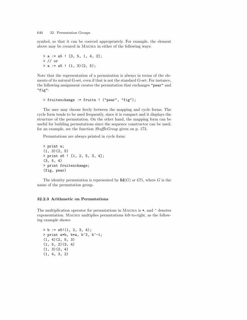
640 32. Permutation Groups
symbol, so that it can be coerced appropriately. For example, the elementabove may be created in Magma in either of the following ways:
> a := s5 ! [3, 5, 1, 4, 2];> // or> a := s5 ! (1, 3)(2, 5);
Note that the representation of a permutation is always in terms of the ele-ments of its natural G-set, even if that is not the standard G-set. For instance,the following assignment creates the permutation that exchanges "pear" and"fig":
> fruitexchange := fruits ! ("pear", "fig");
The user may choose freely between the mapping and cycle forms. Thecycle form tends to be used frequently, since it is compact and it displays thestructure of the permutation. On the other hand, the mapping form can beuseful for building permutations since the sequence constructor can be used;for an example, see the function ShuffleGroup given on p. 173.
Permutations are always printed in cycle form:
> print a;(1, 3)(2, 5)> print s5 ! [1, 2, 5, 3, 4];(3, 5, 4)> print fruitexchange;(fig, pear)
The identity permutation is represented by Id(G) or G!1, where G is thename of the permutation group.
32.2.3 Arithmetic on Permutations
The multiplication operator for permutations in Magma is *, and ^ denotesexponentiation. Magma multiplies permutations left-to-right, as the follow-ing example shows:
> b := s5!(1, 2, 3, 4);> print a*b, b*a, b^2, b^-1;(1, 4)(2, 5, 3)(1, 5, 2)(3, 4)(1, 3)(2, 4)(1, 4, 3, 2)

32.2 The Symmetric Group and Permutations 641
For details of other generic arithmetic operations in groups, including elementorder, element conjugates, and commutators, see Section 29.2.
The function IsEven(g) returns true if g is an even permutation. Forinstance:
> print IsEven(s5!(1, 5)(2, 4, 3)), IsEven(s5!(1, 5)(2, 4));false true
IsOdd(g) behaves analogously.
The function CycleStructure(g) may be used for determining the struc-ture of the cycles of a permutation g. It returns a sequence of pairs in whichthe first component of each tuple is a cycle length and the second componentis the number of cycles with that length. For example, the output below in-dicates that the argument has one cycle of length 5, two cycles of length 2,and 4 fixed points:
> print CycleStructure(Sym(13) ! (2,1)(9,4,7,3,12)(8,10));[ <5, 1>, <2, 2>, <1, 4> ]
Table 32.1. Invariants for permutations
Magma Meaning
CycleStructure(g) Sequence of 2-tuples of form < i, ni >, where ni >0, indicating that g has ni cycles of length i
Fix(g) a ∈ X : ag = aSupport(g) a ∈ X : ag 6= aDegree(g) Cardinality of the support of g, i.e., the number of
points moved by g
IsEven(g) true if g is an even permutation
IsOdd(g) true if g is an odd permutation
These and other invariants for permutations are summarized in Table 32.1.In this table the permutation g is assumed to be an element of a group withnatural G-set X.

642 32. Permutation Groups
32.3 General Permutation Group Constructions
32.3.1 Subgroups and the Permutation Group Constructor
A permutation group H on the set X is a subgroup of the symmetric groupSym(X), and is commonly described in terms of generating permutations.In Magma, H may be created using either of two constructors: the sub-constructor or the special PermutationGroup constructor.
If the sub-constructor is used, then the symmetric group should beplaced on the left side and the generators on the right side. For example,consider the subgroup of the symmetric group on 1, . . . , 6 generated by(1, 2, 5, 6), (3, 4), (1, 6)(2, 5). It may be created using the submagma con-structor as follows:
> s6 := Sym(6);> s6subgp := sub<s6 | (1, 2, 5, 6), (3, 4), (1, 6)(2, 5)>;> print s6subgp;Permutation group s6subgp acting on a set of cardinality 6
(1, 2, 5, 6)(3, 4)(1, 6)(2, 5)
Alternatively, if no reference need be made to the parent symmetric group,then the PermutationGroup constructor is suitable. It has two versions:
PermutationGroup< n | generators >PermutationGroup< T | generators >
where the first version is used if the group has the standard G-set 1, . . . , n,and the second version is used if the G-set of the group corresponds to theenumerated or indexed set T . For instance:
> gp := PermutationGroup<6 | (1,2,5,6), (3,4), (1,6)(2,5)>;> print gp eq s6subgp;true
> fr := "apple", "pear", "fig";> print PermutationGroup< fr | ("pear", "fig") >;Permutation group acting on a set of cardinality 3
(fig, pear)
Of course, the sub-constructor may be used to create a subgroup of anygroup, not just that of the symmetric group. For instance, it may be used

32.3 General Permutation Group Constructions 643
to define the subgroup of s6subgp generated by (1, 6)(2, 5) and the thirdgenerator of s6subgp:
> print sub< s6subgp | (1, 5)(2, 6), s6subgp.3 >;Permutation group acting on a set of cardinality 6
(1, 5)(2, 6)(1, 6)(2, 5)
32.3.2 Standard Groups
Certain permutation groups arise so frequently that standard functions areprovided for their creation. Some of these functions may be found in Section29.1.3. In addition, the functions Sym(n) and Alt(n) provide succinct waysto create the symmetric and alternating groups of degree n.
The following line constructs the cyclic group of order 15 as a permutationgroup:
> a9 := CyclicGroup(GrpPerm, 15);> print a9;Permutation group a9 acting on a set of cardinality 15Order = 15 = 3 * 5
(1, 2, 3, 4, 5, 6, 7, 8, 9, 10, 11, 12, 13, 14, 15)
32.3.3 Projective and Affine Groups
The functions listed in Table 32.2 construct various affine and projectivegroups associated with an n-dimensional vector space V over a finite field Kof cardinality q. For some functions, there are restrictions on the values ofthe arguments; each of the projective group functions require n to be at least2, for instance. Note also that in the case of the unitary groups, PGU(n, q)and PSU(n, q), the group is actually defined over the finite field K = GF(q2).With the exception of the projective Suzuki group (which takes as its singleargument an odd power of 2) these functions take any of the following threepatterns of arguments: n and q; n and K; or V only. In the table only thefirst form is shown.
Each function returns two values: the designated group G acting on thestandard G-set X = 1, . . . , N (where N is the degree of the group) and anindexed set P of vectors of V that define the objects in V that correspond toX. For example, if G is an affine group, then P [i] is the vector correspondingto i ∈ X. Similarly, if G is a projective group, then the vector P [i] generatesthe one-dimensional subspace of V corresponding to i ∈ X.

644 32. Permutation Groups
The standard abbreviations for these groups are available, although thegreek letters Γ , Σ and Ω must be spelt out. Hence, PSL(n, q) may be usedin place of ProjectiveSpecialLinearGroup(n, q)), and PGammaU(n, q)in place of ProjectiveGammaUnitaryGroup(n, q).
Table 32.2. Projective and affine groups
Magma Meaning
AffineGammaLinearGroup(n, q) AΓL(n, q)
AffineSigmaLinearGroup(n, q) AΣL(n, q)
AffineGeneralLinearGroup(n, q) AGL(n, q)
AffineSpecialLinearGroup(n, q) ASL(n, q)
ProjectiveGammaLinearGroup(n, q) PΓL(n, q), n ≥ 2
ProjectiveSigmaLinearGroup(n, q) PΣL(n, q), n ≥ 2
ProjectiveGeneralLinearGroup(n, q) PGL(n, q), n ≥ 2
ProjectiveSpecialLinearGroup(n, q) PSL(n, q), n ≥ 2
ProjectiveGammaUnitaryGroup(n, q) PΓU(n, q), n ≥ 2
ProjectiveSigmaUnitaryGroup(n, q) PΣU(n, q), n ≥ 2
ProjectiveGeneralUnitaryGroup(n, q) PGU(n, q), n ≥ 2
ProjectiveSpecialUnitaryGroup(n, q) PSU(n, q), n ≥ 2
ProjectiveSigmaSymplecticGroup(n, q) PΣSp(n, q), n ≥ 4 and even
ProjectiveSymplecticGroup(n, q) PSp(n, q), n ≥ 4 and even
ProjectiveOmegaPlusGroup(n, q) PΩ+(n, q), n ≥ 4 and even
ProjectiveOmegaMinusGroup(n, q) PΩ−(n, q), n ≥ 4 and even
ProjectiveOmegaGroup(n, q) PΩ(n, q), n ≥ 5 and odd
ProjectiveSuzukiGroup(q) PSz(q), q an odd power of 2
For example:
> K<w> := GF(3^2);> p33, pts := ProjectiveGammaUnitaryGroup(3, 3);> print Degree(p33);28> print pts;@
( 1 0 0), ( 1 w^7 w^3), ( 1 w^6 w^7),( 1 w 2), ( 1 w^5 w), ( 1 w^5 w^3),( 1 1 w^7), ( 1 w^2 w^5), ( 1 1 1),( 1 w^7 w), ( 1 w^3 2), ( 1 2 w^5),( 1 2 w^7), ( 1 1 w^5), ( 1 w w),( 1 w^7 2), ( 1 w^3 w^3), ( 1 w^6 w^5),( 1 w^2 1), ( 1 w^3 w), ( 1 0 w^6),( 0 0 1), ( 1 w w^3), ( 1 w^6 1),

32.3 General Permutation Group Constructions 645
( 1 w^5 2), ( 1 w^2 w^7), ( 1 0 w^2),( 1 2 1)
@> print Order(p33);12096
32.3.4 Product Constructions
Table 32.3. Product constructions for permutation groups
Magma Meaning
DirectProduct(H, K) Direct product of H and K
DirectProduct(Q) Direct product of sequence Q of permutationgroups
TensorProduct(H, K) Wreath product with product action of H and K
TensorProduct(Q) Wreath product with product action of sequenceQ of permutation groups
WreathProduct(H, K) Wreath product with normal action of H and K
WreathProduct(Q) Wreath product with normal action of the of se-quence Q of permutation groups
The standard direct product and wreath product constructions are avail-able in Magma. Table 32.3 lists the relevant functions.
For example, the statement below prints the direct product of Sym(8)and Alt(4):
> print DirectProduct(Sym(8), Alt(4));Permutation group acting on a set of cardinality 12
(1, 2, 3, 4, 5, 6, 7, 8)(1, 2)(9, 10)(11, 12)(9, 10, 11)
and the following statements print the 3-fold iterated wreath product of thecyclic group of order 3:
> Z3 := CyclicGroup(3);> W3 := DirectProduct([Z3 : i in [1..3]]);> print W3;Permutation group W3 acting on a set of cardinality 27
(1, 10, 19)(2, 11, 20)(3, 12, 21)(4, 13, 22)(5, 14, 23)

646 32. Permutation Groups
(6, 15, 24)(7, 16, 25)(8, 17, 26)(9, 18, 27)(1, 4, 7)(2, 5, 8)(3, 6, 9)(1, 2, 3)
> print Order(W3);1594323
32.4 Example: The Group of Symmetries of the Cube
"""
"""
"""
"""
1 234
56
78
Since the group of symmetries of the cube is a convenient example forthe next several sections, it will be introduced here. It will be taken in itsrepresentation as a group cube of permutations of the vertices, numbered 1to 8 (see figure). This group is the subgroup of Sym(8) generated by a =(1, 2, 3, 4)(5, 6, 7, 8), b = (2, 4, 5)(3, 8, 6), c = (1, 5)(2, 6)(3, 7)(4, 8), so it canbe created in Magma as follows:
To perform this example online, type load "I96c32e2";
> cube<a, b, c> := PermutationGroup< 8 |> (1, 2, 3, 4)(5, 6, 7, 8), (2, 4, 5)(3, 8, 6),> (1, 5)(2, 6)(3, 7)(4, 8) >;> print cube;Permutation group cube acting on a set of cardinality 8
(1, 2, 3, 4)(5, 6, 7, 8)(2, 4, 5)(3, 8, 6)(1, 5)(2, 6)(3, 7)(4, 8)

32.5 Basic Operations with Permutation Groups 647
32.5 Basic Operations with Permutation Groups
32.5.1 Computing Images
Let X denote the natural G-set of a permutation group G. If x is a pointof X, the image of x under the permutation g ∈ G is usually written in theexponential notation xg. Consequently, in Magma, x^g denotes the imageof x under the permutation g. An alternative notation is Image(g, x). Forexample, the following calculation shows that the point 4 maps to the point5 when acted on by the permutation ac in cube:
> print 4^(a*c);5
The ^ operator or Image function may also be used to compute the imageof a set or sequence of points. For example, the line below computes the imageof ac on the sequence of points [1, 2, 5]. The resulting sequence shows that 1,2, 5 map to 6, 7, 2, respectively:
> print [1, 2, 5]^(a*c);[ 6, 7, 2 ]
Table 32.4 summarizes the notation for computing images.
Table 32.4. Images under permutations
Magma Meaning
x^g, Image(g, x) Image of point x under permutation g
S^g, Image(g, S) Image of set of points S under permutation g
Q^g, Image(g, Q) Image of sequence of points Q under permutation g
32.5.2 Accessing a Permutation Group
Table 32.5 presents the basic access functions for permutation groups. Tointerpret these functions correctly, it is important to understand how thenatural G-set X for G, the set underlying X, the support of G and its fixed-point set are related. Given a permutation group G with natural G-set X, thefunction Set(X) returns the set underlying X, which is the set on which G isdefined. (The G-set and the underlying set will not usually be distinguishedhere, but since a G-set is a set with structure, it is necessary to apply the

648 32. Permutation Groups
Table 32.5. The permutation representation
Magma Meaning
GSet(G) Natural G-set X for G
Set(X) Enumerated set underlying G-set X
Degree(G) Cardinality of X
Support(G) a ∈ X : ax 6= a, for some x ∈ GFix(G) a ∈ X : ax = a, for all x ∈ GGenerators(G) Set of the defining generators of G
Ngens(G) Number of defining generators of G
Set(G) Set of all the elements of a (small) group G
FormalSet(G) Formal set of all the elements of G
Generic(G) Symmetric group in which G is naturally embedded
Set functor to it in order to access the underlying set as an enumerated set.)The underlying set may be partitioned into two disjoint subsets: the supportof G, which is the set of points that are moved by at least one element of G;and the fixed-point set of G, which is the set of points that are not moved byany element of G. The relationship is illustrated with the following group:
> G := PermutationGroup< 6 | (1,2,4), (4,5,6), (2,4,5) >;> X := GSet(G);> print X;GSet 1 .. 6 > om := Set(X);> print om; 1 .. 6 > print Support(G); 1, 2, 4, 5, 6 > print Fix(G); 3 > print om eq ($1 join $2);true
32.6 Orbits and Transitivity
In this section, the action of G on its natural G-set X will be investigated.At the same time it is convenient to consider the action of G on two derivedG-sets: the set of all k-subsets of X, and the set of all sequences of k distinctelements of X.

32.6 Orbits and Transitivity 649
32.6.1 Transitivity and Regularity
A permutation group G on X is said to be transitive if for any pair of distinctpoints x, y ∈ X, there exists some g ∈ G such that xg = y. The Booleanfunction IsTransitive(G) returns true if G is transitive. For example, thegroup cube defined in Section 32.4 is transitive, since for any given corner ofthe cube there exists a permutation in cube which maps it to any other givencorner:
> print IsTransitive(cube);true
but the subgroup h of cube defined below is intransitive:
> h := sub<cube | a^2, b>;> print h;Permutation group h acting on a set of cardinality 8
(1, 3)(2, 4)(5, 7)(6, 8)(2, 4, 5)(3, 8, 6)
> IsTransitive(h);false
More generally, given a positive integer k, a permutation group G actingon X is k-ply transitive if for any two sequences R and S of k distinct pointsof X, there exists some g ∈ G such that Rg = S. The maximum value d of ksuch that G is k-ply transitive is called the degree of transitivity of G, and isreturned by the function Transitivity(G), The function IsTransitive(G, k)returns true for all k ≤ d.
As an example, the projective general linear group PGL(2, q) is 3-plytransitive:
> print Transitivity(PGL(2, 9));3> print IsTransitive(PGL(2, 9), 2); // 2 le 3 is truetrue
However, given two arbitrary pairs of corners of a cube, it is not alwayspossible to find a permutation of the vertices that maps one pair to the other,because symmetries preserve distance. Therefore the degree of transitivity ofthe group cube is 1:
> print Transitivity(cube);1> print IsTransitive(cube, 1) and not IsTransitive(cube, 2);true

650 32. Permutation Groups
Table 32.6. Transitivity and regularity functions
Magma Meaning
IsTransitive(G) true if G is transitive
Transitivity(G) Degree of transitivity of G
IsTransitive(G, k) true if G acts k-transitively on X
IsSharplyTransitive(G, k) true if G acts sharply k-transitively on X
IsFrobenius(G) true if G is a Frobenius group
IsRegular(G) true if G acts regularly on X
IsSemiregular(G, S) true if G acts semiregularly on the union oforbits S
Table 32.6 lists functions providing information about the transitivity andregularity properties of a permutation group G in its action on its naturalG-set X.
32.6.2 Orbits and Stabilizers
The orbit of a point x ∈ X under a group G is the set xG of all the images ofx. In Magma it may be calculated using either x^G or Orbit(G, x), and itis returned as a G-set. For instance, the following lines calculate some orbitsof the group bgp generated by the element b of cube:
> bgp := sub< cube | b >;> print 1^bgp, 2^bgp;GSet 1 GSet 2, 4, 5
The output shows that 1 is in an orbit by itself, and that 2 is in an orbitcontaining 4 and 5 as well.
Just as in the case of images, an analogous notation is available for com-puting the orbit of a set or sequence. For instance:
> print 1, 2^cube;GSet
1, 5 , 2, 6 , 4, 8 , 7, 8 , 5, 6 , 1, 4 , 6, 7 ,

32.6 Orbits and Transitivity 651
5, 8 , 1, 2 , 3, 7 , 2, 3 , 3, 4
The function Orbits(G) returns all the orbits of G, as a sequence of G-setssuch that the ith G-set contains the points in the ith orbit. For example:
> bgporb := Orbits(bgp);> print bgporb;[
GSet 1 ,GSet 2, 4, 5 ,GSet 3, 6, 8 ,GSet 7
]
Closely related to the idea of an orbit is that of a stabilizer. If x ∈ X, thestabilizer Gx of x in G is the subgroup of G consisting of those permutationsof G that fix x. The function Stabilizer(G, x) returns this subgroup. A stan-dard theorem in permutation group theory states that there is a one-to-onecorrespondence between the cosets of Gx and the orbits of x. Thus, if x ∈ Xand g, h ∈ G, then xg = xh if and only if g and h belong to the same rightcoset of Gx in G.
The functions and operators pertaining to the orbits and stabilizers thatarise from the action of a permutation group G on its natural G-set X aresummarized in Table 32.7.
If H is a subgroup of G, then the function Transversal(G,H) may beused to analyze the cosets of H in G. Its principal return value is an indexedset T of cardinality [G : H] such that T [i] is a right coset representative forthe ith coset of H in G. Its second return value is a mapping φ : G → T suchthat φ(g) = T [i] if and only if g ∈ H ·T [i]. This mapping may be used to findthe canonical coset representative for the coset in which a given g ∈ G lies.
For example, since the orbit of 7 has length 8, the group cube can bepartitioned into 8 cosets, each of which sends 7 to a different point. Thefollowing statements produce canonical coset representatives as an indexedset t:
> stab7 := Stabilizer(cube, 7);> print stab7;Permutation group stab7 acting on a set of cardinality 8

652 32. Permutation Groups
Table 32.7. Orbits and stabilizers
Magma Meaning
a^G,Orbit(G, x) Orbit of point x under G, as a G-set
S^G,Orbit(G, S) Orbit of set S of points under G, as a G-set of subsetsof X
Q^G,Orbit(G, Q) Orbit of sequence Q of points under G, as a G-set ofsequences of points from X
Orbits(G) Sequence Q of G-sets, where Q[i] contains the points inthe ith orbit of G
IsOrbit(G, S) true if subset S of X is a union of orbits of G (i.e., if Sis invariant under G)
Stabilizer(G, x) Stabilizer in G of point x
Stabilizer(G, S) Stabilizer in G of set S
Stabilizer(G, Q) Stabilizer in G of sequence Q
Transversal(G, H) Given group G and subgroup H, returns (i) indexed setT of elements of G forming a right transversal for Gover H (ii) transversal mapping φ : G → T such thatφ(g) = T [i] iff g ∈ H · T [i]
Order = 6 = 2 * 3(2, 4, 5)(3, 8, 6)(3, 6)(4, 5)
> t, m := Transversal(cube, stab7);@
Id(cube),(1, 2, 6, 5)(3, 7, 8, 4),(1, 5)(2, 8)(3, 7)(4, 6),(1, 3, 6)(4, 7, 5),(1, 4, 3, 7, 6, 5)(2, 8),(1, 6)(4, 7),(1, 8)(2, 7),(1, 7)(2, 8)(3, 5)(4, 6)
@Mapping from: GrpPerm: cube to SetIndx: t
Notice that the first element of t is a member of stab7 , so it is the repre-sentative for the coset containing the elements of the subgroup stab7 . Byinspection, the second coset sends 7 to 8, the third coset sends 7 to 3, andso on. The following lines demonstrate this in the case of the element c, bymeans of the transversal mapping m:
> print m(c);(1, 5)(2, 8)(3, 7)(4, 6)> print Index(t, m(c));

32.6 Orbits and Transitivity 653
3> print 7^c eq $1;true
Table 32.8. Conjugacy of G-set elements
Magma Meaning
IsConjugate(G, x, y) true if x, y ∈ X are conjugate in G; if true, alsoreturns a conjugating element
IsConjugate(G, R, S) true if k-subsets R and S of X are conjugate in G; iftrue, also returns a conjugating element
IsConjugate(G, P, Q) true if sequences P and Q, each containing k elementsof X, are conjugate in G; if true, also returns a con-jugating element
It is sometimes useful to know if two elements x, y ∈ X belong to thesame orbit of G and, if so, to find an element g ∈ G such that xg = y. Thefunction IsConjugate(G, x, y) does precisely this, as illustrated in the codebelow. More generally, if Y is any G-set for G, then x, y ∈ Y are said tobe conjugate in G if there exists an element g ∈ G such that xg = y. Thefunctions that determine conjugacy of G-set elements for some G-sets relatedto the natural G-set for G are given in Table 32.8. For example:
> cj, g := IsConjugate(stab7, 3, 5);> print cj;false> cj, g := IsConjugate(stab7, 3, 6);> print cj;true> print g;(2, 5, 4)(3, 6, 8)> print 3 ^ g;6> cj, g := IsConjugate(cube, 2,4, 3,6);> print cj;true> print g;(1, 7)(2, 3)(4, 6)(5, 8)> print 2,4 ^ g; 3, 6
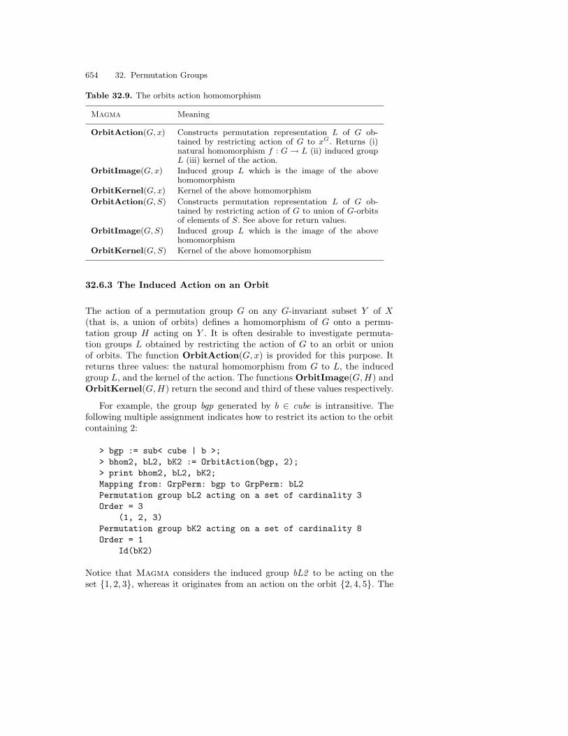
654 32. Permutation Groups
Table 32.9. The orbits action homomorphism
Magma Meaning
OrbitAction(G, x) Constructs permutation representation L of G ob-tained by restricting action of G to xG. Returns (i)natural homomorphism f : G → L (ii) induced groupL (iii) kernel of the action.
OrbitImage(G, x) Induced group L which is the image of the abovehomomorphism
OrbitKernel(G, x) Kernel of the above homomorphism
OrbitAction(G, S) Constructs permutation representation L of G ob-tained by restricting action of G to union of G-orbitsof elements of S. See above for return values.
OrbitImage(G, S) Induced group L which is the image of the abovehomomorphism
OrbitKernel(G, S) Kernel of the above homomorphism
32.6.3 The Induced Action on an Orbit
The action of a permutation group G on any G-invariant subset Y of X(that is, a union of orbits) defines a homomorphism of G onto a permu-tation group H acting on Y . It is often desirable to investigate permuta-tion groups L obtained by restricting the action of G to an orbit or unionof orbits. The function OrbitAction(G, x) is provided for this purpose. Itreturns three values: the natural homomorphism from G to L, the inducedgroup L, and the kernel of the action. The functions OrbitImage(G,H) andOrbitKernel(G,H) return the second and third of these values respectively.
For example, the group bgp generated by b ∈ cube is intransitive. Thefollowing multiple assignment indicates how to restrict its action to the orbitcontaining 2:
> bgp := sub< cube | b >;> bhom2, bL2, bK2 := OrbitAction(bgp, 2);> print bhom2, bL2, bK2;Mapping from: GrpPerm: bgp to GrpPerm: bL2Permutation group bL2 acting on a set of cardinality 3Order = 3
(1, 2, 3)Permutation group bK2 acting on a set of cardinality 8Order = 1
Id(bK2)
Notice that Magma considers the induced group bL2 to be acting on theset 1, 2, 3, whereas it originates from an action on the orbit 2, 4, 5. The

32.7 Systems of Imprimitivity 655
correspondence between these sets may be found by applying bhom2 to asequence consisting of the original points:
> print bhom2([2, 4, 5]);[ 1, 2, 3 ]
Therefore 2 maps to 1, 4 maps to 2, and 5 maps to 3.
The functions pertaining to the orbit action are summarized in Table 32.9.As the table indicates, the homomorphism which maps to the representationobtained by restricting the action of G to a union of orbits may also beconstructed.
32.7 Systems of Imprimitivity
This section is concerned with G-invariant partitions of X.
32.7.1 Blocks and Block Systems
Suppose that G acts transitively on X. A non-empty subset B of X is a blockfor G if for each g ∈ G either Bg = B or Bg ∩ B = φ. The singleton setsx for each x ∈ X are blocks for G, known as the trivial blocks. SupposeB is a block for G, and let Y equal Bg : g ∈ G. Then the sets in Y forma partition of X, and each element of Y is a block for G. The G-invariantpartition Y is called a block system or system of imprimitivity for G, and Ghas a natural action on Y . In Magma, a block system is represented as aG-set whose elements are subsets of X.
If G does not possess a non-trivial system of imprimitivity on X it issaid to be primitive; otherwise it is said to be imprimitive. The functionIsPrimitive(G) tests for this property. For example, the group cube is im-primitive:
> print IsPrimitive(cube);false
If S is a subset of X, then IsBlock(G, S) returns true if S is a block. Forexample, 2, 5 is not a block for cube:
> print IsBlock(cube, 2, 5);false

656 32. Permutation Groups
The function MinimalPartition(G) returns a minimal G-invariant par-tition (block system), where ‘minimal’ means that the partition is non-trivialand that there is no other block system whose blocks are proper subsets ofthese blocks. MaximalPartition(G) works similarly.
For example, in the group cube, the four space diagonals constitute aminimal partition, and the two regular tetrahedra composed of face diagonalsform a maximal partition:
> print MinimalPartition(cube);GSet
2, 8 , 3, 5 , 4, 6 , 1, 7
> print MaximalPartition(cube);GSet
1, 3, 6, 8 , 2, 4, 5, 7
The function MinimalPartition(G) has one parameter, Block. (Thereare no parameters for MaximalPartition.) The default value of Block isan empty set, but if Block is assigned a set of points then the function willreturn a minimal partition satisfying the condition that all the elements ofBlock are in the same block. For example, it was shown above that 2, 5 isnot a block in the group cube. The following assignment constructs a blocksystem for cube in which one block contains 2, 5 and is the smallest suchblock:
> block25 := MinimalPartition(cube: Block := 2, 5);> print block25;GSet
1, 3, 6, 8 , 2, 4, 5, 7
In this partition, 2 and 5 are together in the second block.
The function MinimalPartitions(G) constructs all the minimal blocksystems of G, as a sequence of G-sets. Any system of imprimitivity can bewritten as a union of blocks of one of the minimal systems. For example, theoutput below shows that cube has two minimal block systems:

32.7 Systems of Imprimitivity 657
To perform this example online, type load "I96c32e3";
> blkscube := MinimalPartitions(cube);> print blkscube;[
GSet 2, 8 , 3, 5 , 4, 6 , 1, 7
,GSet
1, 3, 6, 8 , 2, 4, 5, 7
]
Each G-set describes a system of imprimitivity. In this example, the systemshappen to be the minimal and maximal partition already constructed.
Table 32.10. Block functions
Magma Meaning
IsPrimitive(G) true if G is primitive
IsBlock(G, S) true if set of points S is a block for G
MinimalPartition(G) A minimal block system for G; if a set of points isassigned to the parameter Block, then one of theblocks must contain that set
MaximalPartition(G) A maximal block system for G
MinimalPartitions(G) Sequence containing the minimal block systems of G
The functions pertaining to blocks and block systems are summarized inTable 32.10.
32.7.2 The Induced Action on a Block System
Given any block system Y , BlocksAction(G, Y ) constructs the homomor-phism of G onto the group obtained by the action of G on the blocks of Y . Asis the case with the homomorphism functions discussed above, this functionreturns three values: the natural homomorphism G → L, the induced groupL, and the kernel of the action. The functions for obtaining the blocks actionare summarized in Table 32.11.

658 32. Permutation Groups
Table 32.11. The blocks action homomorphism
Magma Meaning
BlocksAction(G, Y ) Constructs permutation representation L of G inducedby action of G on blocks of Y . Returns (i) naturalhomomorphism f : G → L (ii) induced group L (iii)kernel of the action
BlocksImage(G, Y ) Image L of the above homomorphism
BlocksKernel(G, Y ) Kernel of the above homomorphism
For example, when BlocksAction is applied to the first system ofblkscube (defined above), the induced group cubeL2 is an order-24 subgroupof S4, so it must be the whole of S4. The four objects on which cubeL2 actsare the four blocks in the first minimal system of imprimitivity:
To perform this example online, type load "I96c32e4";
> cubef2, cubeL2, cubeK2 := BlocksAction(cube, blkscube[1]);> print cubef2, cubeL2, cubeK2;Mapping from: GrpPerm: cube to GrpPerm: cubeL2Permutation group cubeL2 acting on a set of cardinality 4Order = 24 = 2^3 * 3
(1, 2, 3, 4)(2, 4, 3)(3, 4)
Permutation group cubeK2 acting on a set of cardinality 8Order = 2
(1, 7)(2, 8)(3, 5)(4, 6)
The correspondence between the block system and the G-set of the in-duced group may be calculated as follows:
> print [ < bl, cubef2(bl) > : bl in blkscube[1] ];[
< 2, 8 , 2 >,< 3, 5 , 3 >,< 4, 6 , 4 >,< 1, 7 , 1 >
]
The output above shows that the block 2, 8 corresponds to point 2 in thecubeL2 , the block 3, 5 corresponds to point 3 in cubeL2 , and so on.

32.7 Systems of Imprimitivity 659
32.7.3 Example: A Reduction Algorithm
The following code illustrates the role of actions on orbits and block systemsin permutation group algorithms. It implements an unpublished algorithmdue to Bill Kantor for constructing the p-core of a permutation group G.Whereas the complete algorithm is designed to find a maximal normal p-subgroup of G, the version presented here determines whether or not G con-tains a non-trivial elementary abelian normal subgroup, and, if so, constructsit. The algorithm applies OrbitAction to reduce to a transitive group T ,then BlocksAction to reduce to a primitive group P . If the kernel K of thehomomorphism τ : T → P is non-trivial then the algorithm is called recur-sively on K. If this does not yield an elementary abelian normal subgroup,the algorithm is applied recursively to CG(K).
pSubgroup := func< G, p |sub< G | x ^ (Order(x) div p): x in Generators(G) > >;
TransitiveReduction := function(G)/*Returns: (i) natural homomorphism phi: G -> H of G onto atransitive constituent H, (ii) H, (iii) kernel of phi.*/
if IsTransitive(G) thenreturn IdentityHomomorphism(G), G, sub<G |>;
elsereturn OrbitAction(G, Rep(Support(G)));
end if;end function;
PrimitiveReduction := function(G)/*Returns: (i) natural homomorphism tau: G -> H oftransitive group G onto a primitive component H,(ii) H, (iii) kernel of tau.*/
S := MaximalPartition(G);if IsPrimitive(G) then
return IdentityHomomorphism(G), G, sub<G |>;else
return BlocksAction(G, S);end if;
end function;
AbelianNormalSubgroup := function(G)/*

660 32. Permutation Groups
Returns a non-trivial elementary abelian normal subgroupof G if one exists, otherwise the trivial subgroup.*/
if IsTrivial(G) thenreturn G;
end if;phi, T, KT := TransitiveReduction(G);tau, P, KP := PrimitiveReduction(T);K := KP @@ phi;if IsTrivial(K) then
return (EARNS(P) @@ tau) @@ phi;else
Z := Centre(K);if not IsTrivial(Z) then
return pSubgroup(Z, FactoredOrder(Z)[1][1]);end if;A := $$(K);if IsTrivial(A) then
A := $$(Centralizer(G, K));if IsTrivial(A) then
return A;end if;
end if;Z := Centre(NormalClosure(G, A));return pSubgroup(Z, FactoredOrder(Z)[1][1]);
end if;end function;
32.8 General G-sets
32.8.1 Construction of a G-set
It is convenient to distinguish three types of G-set for a permutation groupG. As noted at the beginning of the chapter, the set on which G is definedis termed the natural G-set and the action of G on X is called the naturalaction of G.
A general G-set for the group G is an arbitrary set Y togther with amapping φ : Y ×G → Y satisfying
((y, g)φ, h)φ = (y, gh)φ and (y, 1G)φ = y
for all y ∈ Y and all g, h ∈ G. Now, let A be some set. A derived set of A isdefined (recursively) as follows:

32.8 General G-sets 661
– A subset of A is a derived set;
– A set of k-subsets of A, k-sequences of A, or ordered partitions of A is aderived set;
– A subset of a Cartesian product of derived sets of A is a derived set.
The natural action of G on X induces a natural action on the G-closure Yof any derived set of X. Such a set Y is also a G-set. For example, a subsetof X is a G-set for G if and only if it is a union of orbits for G. A derived setof the natural G-set X for G will be called a derived G-set for G.
For a permutation group G defined on X, Magma allows the user todefine an arbitrary number of additional G-sets. This mechanism enables theuser to work with different actions of G without explicitly having to formthe homomorphic image of G with respect to each action. Operations maybe specified in terms of G.
In Magma, a general G-set may be constructed using the functionGSet(G,Y, f), where f is a mapping from the Cartesian product of Y andG to Y . If Y ′ is the closure of Y under f (usually Y = Y ′), then f must bean action of G on Y ′, in the sense defined in Section 32.1. The G-set will beconstructed on Y ′.
To illustrate the use of this function, let V be an n-dimensional vectorspace defined over GF(2) and let G be a permutation group of degree 2n de-fined on the G-set 1, 2, . . . , 2n. The action of G on V is obtained by estab-lishing a bijection between V and X such that v ∈ V is mapped to 1+N(V ),where N(v) is the integer obtained by taking the components of v to be thedigits of the base-2 representation of an integer. The function VSpaceActionbelow produces the required G-set, and returns the corresponding action.
VSpaceAction := function(G, V);Z := IntegerRing();d := Dimension(V);
VecToInt := func< v |1 + &+[ Z!v[i]*(2^(i-1)) : i in [1..d] ] >;
IntToVec := func< n, V |V ! (q cat [ 0 : i in [1..(d-#q)] ])
where q is IntegerToSequence(n-1, 2) >;
Y := Set(V);Y_Act := map< car<Y, G> -> Y |
t :-> IntToVec(VecToInt(t[1])^t[2], V) >;W := GSet(G, Y, Y_Act);return Action(G, W);

662 32. Permutation Groups
end function;
For instance, let V be the 3-dimensional vector space over GF(2) and G bePSL(2, 7):
> G := PSL(2, 7);> V := VectorSpace(GF(2), 3);> f := VSpaceAction(G, V);> H := Image(f);> print H;Permutation group H acting on a set of cardinality 8Order = 168 = 2^3 * 3 * 7
((0 1 0), (1 0 1), (0 1 1))((1 1 0), (0 0 1), (1 1 1))((0 0 0), (1 1 1), (1 0 0))((1 1 0), (0 0 1), (1 0 1))
> x := Random(G); print x;(1, 2, 6, 8, 4, 5, 3)> print [ < v, v^(x@f)> : v in V ];[
<(0 0 0), (1 0 0)>,<(1 0 0), (1 0 1)>,<(0 1 0), (0 0 0)>,<(1 1 0), (0 0 1)>,<(0 0 1), (0 1 0)>,<(1 0 1), (1 1 1)>,<(0 1 1), (0 1 1)>,<(1 1 1), (1 1 0)>
]> y := Random(H); print y;((0 0 0), (1 0 0), (0 0 1), (0 1 0), (1 0 1), (0 1 1),(1 1 0))> print [ < a, a^(y@@f)> : a in GSet(G) ];[ <1, 2>, <2, 5>, <3, 6>, <4, 1>, <5, 3>, <6, 7>, <7, 4>,<8, 8> ]
A derived G-set may be created using the function GSet(G,S), where Sis a derived set of the natural G-set of G. This function forms the closureY of S under G, and takes the action of G on Y to be that induced by theaction of G on X. In the example below, GSet(G, S) will be used to constructa representation of the group PSL(3, 4) on flags (point-line pairs), startingwith its action on projective points. In order to construct the flags, it is firstnecessary to find a line. If H is the stabilizer of a point α in PSL(3, 4) in itsaction on projective points, then a line consists of α together with the pointsin any non-trivial orbit of O2(G).
> G := ProjectiveSpecialLinearGroup(3, 4);

32.8 General G-sets 663
> O2 := pCore(Stabilizer(G, 1), 2);> print Order(O2);16> flag := < 1, Orbit(O2, 2) >;> print flag;<1, GSet 2, 5, 15, 17 >> flags := GSet(G, Orbit(G, flag));> print #flags;105
Table 32.12. Access functions for G-sets
Magma Meaning
Action(Y ) Mapping giving action on G-set Y
Degree(G, Y ) Cardinality of G-set Y
Group(Y ) Group for G-set Y
Set(Y ) Set underlying G-set Y
Support(Y ) Support of G-set Y
Labelling(G) Indexed set giving internal mapping of natural G-setof G onto standard G-set 1, . . . , n
The elementary access functions for G-sets are listed in Table 32.12.
32.8.2 Orbits and Stabilizers for General G-Sets
The functions for computing images, orbits and stabilizers and related ob-jects that were presented earlier in this chapter have a generalized formin which the second argument is the required G-set. As usual, supposethat G is a permutation group defined on X, Y is a G-set of G, andy ∈ Y . Then Image(g, Y, y) constructs the image of y under g ∈ G,Orbit(G,Y, y) forms the orbit of y, Orbits(G,Y ) constructs all G-orbitson Y , and Stabilizer(G,Y, y) finds the subgroup of G that fixes y. Theseand related functions are listed in Table 32.13.
Some of these functions are illustrated using the action of PSL(3, 4) onflags constructed above:
> print Image(G.2, flag);<8, 1, 3, 9, 12 >> x := <21, 2, 7, 8, 11 >;> y := <11, 2, 7, 8, 21 >;> print IsConjugate(G, flags, x, y);

664 32. Permutation Groups
Table 32.13. Orbits and stabilizers on G-sets
Image(g, Y, y) Orbit(G, Y, y) Orbits(G, Y, y)
Fix(g, Y ) Fix(G, Y ) Stabilizer(G, Y, y)
IsPrimitive(G, Y ) Transitivity(G, Y ) IsConjugate(G, Y, y, z)
IsTransitive(G, Y ) IsTransitive(G, Y, k) IsSharplyTransitive(G, Y, k)
IsRegular(G, Y ) IsSemiregular(G, Y ) IsSemiregular(G, Y, S)
true(1, 17, 5)(3, 12, 10)(4, 16, 20)(6, 19, 13)
(8, 21, 11)(9, 18, 14)> print #Orbit(G, flags, flag);105> print IsPrimitive(G, flags);false
32.8.3 The Induced Action on a G-set
Table 32.14. Homomorphism induced by an action on a G-set
Magma Meaning
Action(G, Y ) Homomorphism of G onto GY
ActionImage(G, Y ) Image of Action(G, Y )
ActionKernel(G, Y ) Kernel of Action(G, Y )
IsFaithful(G, Y ) true if G acts faithfully on Y
If G is a permutation group defined on X and Y is a G-set for G, thefunction Action(G,Y ) constructs the homomorphism φ : G → GY , whereGY denotes the representation of G given by its action on Y . It also returnsthe image and kernel of the homomorphism. The functions for the inducedaction are summarized in Table 32.14.
Continuing with the action of PSL(3, 4) on flags, the following lines con-struct the image FG of G under this action explicitly. Then the stabilizer of< 21, 2, 7, 8, 11 > is constructed in both G and FG , and the two stabilizersare compared:
> phi, FG, ker := Action(G, flags);> print FG;Permutation group FG acting on a set of cardinality 105Order = 20160 = 2^6 * 3^2 * 5 * 7

32.9 Primitive Groups and the O’Nan-Scott Theorem 665
> x := <21, 2, 7, 8, 11 >;> Gstab := Stabilizer(G, x[1]) meet Stabilizer(G, x[2]);> print Degree(Gstab), Order(Gstab);21 192> FGstab := Stabilizer(FG, x);> print Degree(FGstab), Order(FGstab);105 192> print FGstab@@phi eq Gstab;true
32.9 Primitive Groups and the O’Nan-Scott Theorem
Given an arbitrary permutation group, the OrbitAction and BlocksActionfunctions enable the user to construct a chain of normal subgroups such thatthe quotients of successive terms are primitive.
Magma contains tools which provide a detailed description of a primitivepermutation group according to the structural description provided by theO’Nan-Scott theorem [DiM96]. In this section, only a few of the availabletools will be described; the interested reader should consult the Handbook fora more complete description.
32.9.1 Recognition of the Alternating and Symmetric Groups
It is frequently desirable to be able to recognize that a permutation groupG defined on X contains Alt(X), without computing the order of G. Thefunction IsAltsym(G) returns true if G contains Alt(X), and the func-tions IsAlternating(G) and IsSymmetric(G) are minor variants that re-turn true if G is Sym(X) or Alt(X) respectively. If G does contain Alt(X),these tests will usually detect the fact very rapidly, even for groups havingdegrees in the millions. For example:
> G := Sym(1000000);> H := sub< G | Random(G), Random(G) >;> time print IsAltsym(H);trueTime: 6.939
These functions operate by examining a number of random elements ofG in an attempt to determine whether G is primitive, and, if so, whetherG contains elements that are not contained in a primitive group other thanSym(X) and Alt(X). If this attempt does not succeed after a certain amount

666 32. Permutation Groups
of effort, a Schreier algorithm is invoked to compute the order of G, so as tosettle the issue definitively.
32.9.2 Primitive Groups with Abelian Socle
Primitive groups divide naturally into two classes, depending upon whetheror not their socle is abelian. If the primitive group G possesses an abeliansocle, then it acts regularly and is unique. The function EARNS(G) returnsthe unique elementary abelian regular normal subgroup N of G, if such asubgroup exists, or the trivial group if not. The stabilizer Gx of any point x inG is a complement for N , and G/N is isomorphic to Gx. Consequently, there isa homomorphism φ : G → Gx. This homomorphism, its image and its kernelare constructed by the functions AffineAction(G), AffineImage(G), andAffineKernel(G). (Of course, AffineKernel(G) returns the same subgroupas EARNS(G).) For example:
> G := PermutationGroup< 16 |> (1,15,7,5,12)(2,9,13,14,8)(3,6,10,11,4),> (1,7)(2,11)(3,12)(4,13)(5,10)(8,14),> (1,16)(2,3)(4,5)(6,7)(8,9)(10,11)(12,13)(14,15) >;> print Order(G);11520> N := EARNS(G);> print N;Permutation group N acting on a set of cardinality 16Order = 16 = 2^4
(1, 2)(3, 16)(4, 7)(5, 6)(8, 11)(9, 10)(12, 15)(13, 14)(1, 7)(2, 4)(3, 5)(6, 16)(8, 14)(9, 15)(10, 12)(11, 13)(1, 13)(2, 14)(3, 15)(4, 8)(5, 9)(6, 10)(7, 11)(12, 16)(1, 16)(2, 3)(4, 5)(6, 7)(8, 9)(10, 11)(12, 13)(14, 15)
> print IsRegular(N);true> f, H := AffineAction(G);> print H;> print FactoredOrder(H);[ <2, 4>, <3, 2>, <5, 1> ]> print CompositionFactors(H);
G| Cyclic(2)*| Alternating(6)1
> print existsT : T in NormalSubgroups(H) | T‘order eq 2;false

32.9 Primitive Groups and the O’Nan-Scott Theorem 667
The final statement establishes that H cannot be Z2 × Alt(6) and so mustbe Sym(6). It may be concluded that G consists of Sym(6) extended by theelementary abelian group of order 16.
32.9.3 Primitive Groups with Non-Abelian Socle
Suppose that G is a primitive group with non-abelian socle N . Then N is adirect product of isomorphic simple groups so that N = S1×S2× . . . Sr. Thefunction Socle(G) returns the socle of G. It is well known that a primitivegroup has at most two minimal normal subgroups and these may be computedusing the function MinimalNormalSubgroups(G).
A number of related functions allow the user to analyze the socle in differ-ent ways: the function SocleFactors(G) returns the sequence [S1, S2, . . . Sr];SocleFactor(G) returns a single factor of N ; and SocleSeries(G) returnsa composition series for the socle N of G. The group G acts on S1, S2, . . . Sr
by conjugation. The group thereby induced is returned by SocleImage(G),while the kernel of this action is given by SocleKernel(G).
These functions are illustrated by considering the tensor product ofSym(5) and Alt(5) with product action. Recall that product action results ina primitive group.
> G := TensorProduct(Sym(5), Alt(5));> print Order(G);1492992000000> print FactoredOrder(G);[ <2, 17>, <3, 6>, <5, 6> ]> N := Socle(g); print N;Permutation group N acting on a set of cardinality 3125Order = 777600000 = 2^10 * 3^5 * 5^5> Fac := SocleFactor(G); print Fac;Permutation group Fac acting on a set of cardinality 3125Order = 60 = 2^2 * 3 * 5> Facs := SocleFactors(G);> print Facs;[
Permutation group acting on a set of cardinality 3125Order = 60 = 2^2 * 3 * 5,Permutation group acting on a set of cardinality 3125Order = 60 = 2^2 * 3 * 5,Permutation group acting on a set of cardinality 3125Order = 60 = 2^2 * 3 * 5,Permutation group acting on a set of cardinality 3125Order = 60 = 2^2 * 3 * 5,

668 32. Permutation Groups
Permutation group acting on a set of cardinality 3125Order = 60 = 2^2 * 3 * 5
]> NSer := SocleSeries(G);> print NSer;[
Permutation group acting on a set of cardinality 3125Order = 60 = 2^2 * 3 * 5,Permutation group acting on a set of cardinality 3125Order = 3600 = 2^4 * 3^2 * 5^2,Permutation group acting on a set of cardinality 3125Order = 216000 = 2^6 * 3^3 * 5^3,Permutation group acting on a set of cardinality 3125Order = 12960000 = 2^8 * 3^4 * 5^4,Permutation group acting on a set of cardinality 3125Order = 777600000 = 2^10 * 3^5 * 5^5
]> NIm := SocleImage(G); print NIm;Permutation group NIm acting on a set of cardinality 5Order = 60 = 2^2 * 3 * 5
(1, 2, 4)(1, 3, 5)
> NKer := SocleKernel(g); print NKer;Permutation group NKer acting on a set of cardinality 3125Order = 2^15 * 3^5 * 5^5> M, tau := GModule(G, SocKer, N);> print M;GModule M of dimension 5 over GF(2)> NKerSer := [ S@@tau : S in CompositionSeries(M) ];> print NKerSer;[
Permutation group acting on a set of cardinality 3125Order = 2^14 * 3^5 * 5^5,Permutation group SocKer acting on a set ofcardinality 3125Order = 2^15 * 3^5 * 5^5
]
From the working above, the structure of the group is clearly revealed. Thesocle N consists of five copies of Alt(5), each acting on 3125 points. Thegroup G acts as Alt(5) on the set of socle factors while the kernel of thisaction contains the socle N of G as a subgroup of index 25. This section iselementary abelian and so can be regarded as a G-module. This G-modulesplits into a one-dimensional submodule and a four dimensional submodule.

32.10 Base and Strong Generating Sets 669
Pulling these submodules back into G completes the determination of a chiefseries for G.
32.10 Base and Strong Generating Sets
The material in this short section is concerned with the construction of a spe-cial representation of a permutation group that is central to most permutationgroup algorithms. In most situations the user need not be concerned aboutthis representation, but its construction may dominate the execution timefor many algorithms. Knowledge of the material presented here can lead tosignificantly faster computation in many circumstances. However, this treat-ment is only superficial, and the serious user will need to study the ideas atmuch greater depth elsewhere.
Computing structural information for a permutation group G acting on Xrequires, in most cases, a representation of the set of elements of G. Magmarepresents this set by means of a base and strong generating set, or BSGS, forG. A base B for G is a sequence of distinct points from X with the propertythat the identity is the only element of G that fixes B pointwise. A base Bof length n determines a sequence of subgroups G(i), 0 ≤ i ≤ n, where G(i)
is the stabilizer of the first i− 1 points of B. Given a base B for G, a subsetS of G is said to be a strong generating set for G if G(i) = S ∩ G(i), fori = 1, . . . , n.
Almost all of the structure algorithms for permutation groups presup-pose the availability of a BSGS for the group in question. Once it has beencomputed for a particular group, Magma will save it for possible future use.Since the computation of a BSGS may be very expensive, a number of dif-ferent algorithms have been developed; their family is known generically asSchreier-Sims algorithms. The best choice of algorithm usually depends uponwhat is known about the group. If the user does not intervene, Magma willautomatically choose which Schreier algorithm to invoke. However, for verylarge groups, it is often possible for the user to reduce the computation timegreatly, through the selection of a Schreier algorithm appropriate to the groupunder consideration.
The procedure BSGS(G) constructs a base and strong generating set forthe group G using the default algorithm choices.
The procedure SimsSchreier(G) constructs a BSGS for G using thestandard Schreier-Sims algorithm. This algorithm is mainly appropriate forgroups of very small degree (less than 100).

670 32. Permutation Groups
The procedure SolubleSchreier(G) is designed to take advantage of thespecial structure of soluble groups, and is the recommended algorithm for theBSGS if G is known to be soluble.
The procedure RandomSchreier(G) constructs a BSGS for G using arandom choice for potential strong generators rather than systematically con-structing all Schreier generators. There is no guarantee that the algorithmwill have constructed a correct BSGS upon completion, so the user may wishto test the result using Verify (see below). The stopping criterion is con-trolled by two independent parameters taking positive integer values. Thefirst, Max (default 100), specifies that at most Max random elements are tobe tried as potential strong generators; the second, Run (default 20), speci-fies that the algorithm is to terminate after a run of Run successive randomelements has failed to enlarge the strong generating set. RandomSchreieris particularly useful when the order of G is known in advance. The usershould first set the order of G using AssertAttribute(G, "Order", n) andthen run RandomSchreier. If an order is set for G, the random algorithmwill continue until a group of that order has been constructed.
The procedure ToddCoxeterSchreier(G) applies an algorithm devel-oped by Leon and Sims. It employs a Todd-Coxeter method to select newstrong generators and prove correctness. This is the algorithm of choice ifthe random Schreier is not applicable and the degree lies between 100 and10 000.
The procedure Verify(G) verifies the correctness of a BSGS that has beenconstructed by the random Schreier. It was developed by Brownie, Cannonand Sims and is based on ideas used by Sims in his construction of the Lyonsand O’Nan simple groups. This algorithm is designed for groups having degreein excess of 100 000.
For example, the code below applies RandomSchreier(G) to a largewreath product, whose order is known by construction:
> G := WreathProduct(Sym(42), Alt(8));> AssertAttribute(G, "Order",> Factorial(42)^8 * (Factorial(8) div 2));> RandomSchreier(G);

33. Matrix Groups
Techniques for computing with matrix groups are less well developed thanthose for permutation groups. While a matrix group may be created overany ring R satisfying the condition that Magma is able to invert elementsof Matn(R), the types of computation that are possible depend heavily onthe coefficient ring, the dimension of the group and its cardinality (especiallywhether finite or infinite). In order to get a rough understanding of the pos-sibilities, it is important to distinguish three computationally distinct classesof matrix groups.
The first class comprises finite matrix groups G defined over a field oreuclidean ring, where G satisfies the following conditions:
– G has moderate degree;
– G has a short orbit ∆ in its action on the natural module and ∆ can belocated by Magma.
(By short orbit is meant an orbit having cardinality at most 1,000,000). Notethat G does not have to act faithfully on ∆. For this class of groups, a sta-bilizer chain representation similar to that used for permutation groups isemployed (the BSGS representation). A wide range of structural computa-tions may be performed on members of this class of group.
The second class consists of matrix groups defined over finite fields. Acomputational approach to the analysis of such groups based on Aschbacher’sclassification of the maximal subgroups of GL(n, q) is under development byHolt, Leedham-Green, O’Brien, Praeger, P. Neumann and others. This ma-chinery has the capability of determining the order and composition factorsof many groups in this class having degree up to 200.
The third class comprises those matrix groups for which it is not possibleto construct a Structure Normal Form (SNF). These groups include all infinitematrix groups and finite groups of large degree that do not fall into thefirst class. While element operations are available for this class of groups, nooperations that depend upon testing membership of subgroups are supported.

672 33. Matrix Groups
33.1 The General Linear Group and Its Elements
33.1.1 Creating the General Linear Group
A matrix group over the ring R is a subgroup of the general linear groupGL(n,R) (the group of all invertible n× n matrices with entries in the ringR). Thus, GL(n,R) will be the generic group for all n×n matrix groups overR. This group will be created by the function GeneralLinearGroup(n, R),usually abbreviated GL(n,R). Note that this function only creates a shellstructure: it does not construct actual generators for GL(n,R). If some sub-sequent operation requiring the generators is invoked, they will be automat-ically constructed only in the case where R is a finite field GF (q). For allother coefficient rings it is necessary for the user to supply his or her owngenerators. The category for subgroups of GL(n, R) is GrpMat.
For example, the group G5 below is the general linear group of degree 3over the finite field of five elements:
> gf5 := GF(5);> G5 := GeneralLinearGroup(3, gf5);> print G5;GL(3, GF(5, 1))
At this point, G5 is a “shell structure” that contains the parameters ofgeneral linear group but no generators. In the example below, printing theorder has the effect of creating generators so that so the print-statementgives more information than it did previously:
> print #G5;1488000> print G5;MatrixGroup(3, GF(5)) of order 1488000 = 2^7 * 3 * 5^3 * 31Generators:
[2 0 0][0 1 0][0 0 1]
[4 0 1][4 0 0][0 4 0]
The possible categories of coefficient ring for matrix groups in Magmainclude finite fields, number fields, function fields, p-adic fields, the ring ofintegers ZZ, quotient rings ZZ/mZZ and univariate polynomial rings over a field.

33.1 The General Linear Group and Its Elements 673
33.1.2 Representation of Matrices
An element of a matrix group may be created by building a sequence con-taining its entries listed in row-major order, and coercing this sequence intothe group. This is the same method for matrix creation as is used in the caseof matrix spaces and matrix algebras. For example:
> g := G5 ! [3, 1, 2, 2, 4, 4, 2, 0, 3];> print g;[3 1 2][2 4 4][2 0 3]
Here Magma has automatically coerced the integer terms of the sequence intoelements of the finite field gf5 . The function for decomposing a matrix g intothe corresponding sequence of ring elements, is ElementToSequence(m) orEltseq(m):
> print Eltseq(g);[ 3, 1, 2, 2, 4, 4, 2, 0, 3 ]
The identity matrix of a group G may be constructed as Identity(G), orG!1.
33.1.3 Arithmetic on Matrices
The standard multiplicative operators apply to elements of matrix groups: ∗and ^. An inverses is found by exponentiation to the power −1.
> h := G5 ! [3, 0, 0, 0, 4, 2, 0, 2, 3];> print g * h, h * g;[4 3 3][1 4 0][1 1 4]
[4 3 1][2 1 2][0 3 2]
> print g ^ 10;[0 3 0][2 0 0][2 4 1]

674 33. Matrix Groups
> print h ^ -1;[2 0 0][0 1 1][0 1 3]
It is possible to access entry i, j or row i of a matrix group element g,using the syntax g[i, j] or g[i]. For instance:
> print g[2];(2 4 4)> print g[2,3];4
However, it is not permitted to modify a matrix by redefining entries (asis done with sequences), since, in general, the result will not be an elementof the group. If the user needs to perform such an operation, the matrixshould be first converted to a sequence using Eltseq, the sequence modifiedas required and then coerced back into the group.
Multiplication involving matrices is possible when the two matrices areelements of (or coercible into) a common matrix group, and also in some othercases when the coefficient rings are compatible and the number of columnsof the first matrix equals the number of rows of the second matrix. If theother matrix is from a matrix ring then it will be possible. If the first matrixis from a matrix space or suitably-sized vector space (or module) and thesecond is from a matrix group it will be possible; this is an instance of thegroup acting on the space.
33.1.4 The Order of a Matrix
The order of an element g of a matrix group is returned by the functionOrder(g). There are several points to note about the Magma facilities fordetermining the order of a matrix. Firstly, if g has infinite order, the functionwill not recognize this fact and may never return.
The analysis of matrix groups over finite fields makes heavy use of beingable to locate elements having certain orders. For this case, Magma employs avery efficient algorithm due to Leedham-Green which is capable of computingthe order of elements in groups having degree up to 1000. Since the factor-ization of the orders may be very difficult in large groups, an alternate ver-sion is available for when the factored order is required: FactoredOrder(g).This exploits the fact that the manner in which the order is determined pro-duces a partial factorization. The example below sets up the orthogonal group

33.1 The General Linear Group and Its Elements 675
Ω+(200, 4), produces a random element of the group and computes its order,both as an integer and as a factorization sequence.
> G := OmegaPlus(200, 4);> RP := RandomProcess(G);> x := Random(RP);> time Order(x);1286039129078980091566889421260550476237553615698059806510Time: 27.649> time FactoredOrder(x);[ <2, 1>, <3, 2>, <5, 1>, <7, 1>, <11, 1>, <17, 1>,<31, 1>, <3855260977, 1>, <64082150767423457, 1>,<1425343275103126327372769, 1>]Time: 26.689
Since the Leedham-Green algorithm requires factorization of large inte-gers, the order algorithm may sometimes fail or be very expensive. For someapplications, it suffices to obtain a multiple of the order. The boolean-valuedparameter Proof for functions Order and FactoredOrder allows the userto specify that difficult integer factorizations are not to be attempted so thatthe value returned may be a multiple of the true order of g. In this case, asecond boolean value is returned: true if the order is known to be correctand false if it may be a multiple of the true order.
The projective order of an element g of a matrix group is the least pos-itive integer n such that gn = λI, where I is the identity matrix. FunctionsProjectiveOrder and FactoredProjectiveOrder return the projective or-der or factored projective order, respectively. The scalar λ is returned as asecond return value by both functions.
33.1.5 Matrix Invariants and Canonical Forms
Many of the operations provided for elements of matrix rings may also beapplied to the elements of matrix groups (see Table 33.1 (p. 676)). The variouscanonical forms may be computed over a field, while MinimalPolynomialworks for any field and ZZ. Operations such as Adjoint and Transpose,when applied to an element of the group G, return their result as an elementof the matrix ring in which G is naturally embedded. See also Table 28.4 (p.536) and Table 28.5 (p. 539).

676 33. Matrix Groups
Table 33.1. Properties of a matrix regarded as a linear transformation
Adjoint(g) JordanForm(g)
CharacteristicPolynomia(g) MinimalPolynomial(g)
Determinant(g) PrimaryRationalForm(g)
Eigenspace(g, a) PrimaryInvariantFactors(g)
Eigenvalues(g) RationalForm(g)
HessenbergForm(g) Transpose(g)
InvariantFactors(g) Trace(g)
33.2 General Matrix Group Constructions
A matrix group is always viewed by Magma as being a subgroup of GL(n, R).The formal way of defining a matrix group is therefore to construct it explic-itly as a subgroup of GL(n,R). As usual, a constructor is provided that allowsthe two steps to be performed by a single statement.
33.2.1 Constructing Subgroups
Given a subgroup G of GL(n,R), the sub-constructor applied to G has theform
sub< G | generator specification >
where the generators for the subgroup are given as a list whose terms maybe any of the following: element of G, element of Matn(R) belonging to G,sequence defining a matrix of G, a subgroup of G, or a set or sequence or anyof the above.
For instance, consider the group G6 of 2× 2 matrices over ZZ6 generatedby the matrices (
5 15 0
)and
(5 51 2
)
> Z6 := ResidueClassRing(6);> GL2Z6 := GL(2, Z6);> G6 := sub< GL2Z6 | [5, 1, 5, 0 ], [5, 5, 1, 2] >;> print G6;MatrixGroup(2, Residue class ring of integers modulo 6)Generators:
[5 1][5 0]
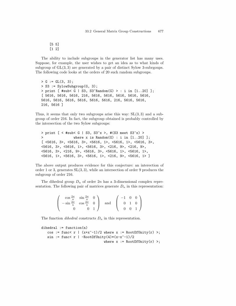
33.2 General Matrix Group Constructions 677
[5 5][1 2]
The ability to include subgroups in the generator list has many uses.Suppose, for example, the user wishes to get an idea as to what kinds ofsubgroup of GL(3, 3) are generated by a pair of distinct Sylow 3-subrgoups.The following code looks at the orders of 20 such random subgroups.
> G := GL(3, 3);> S3 := SylowSubgroup(G, 3);> print [ #sub< G | S3, S3^Random(G) > : i in [1..20] ];[ 5616, 5616, 5616, 216, 5616, 5616, 5616, 5616, 5616,5616, 5616, 5616, 5616, 5616, 5616, 216, 5616, 5616,216, 5616 ]
Thus, it seems that only two subgroups arise this way: SL(3, 3) and a sub-group of order 216. In fact, the subgroup obtained is probably controlled bythe intersection of the two Sylow subgroups:
> print [ < #sub< G | S3, S3^x >, #(S3 meet S3^x) >> where x is Random(G) : i in [1..20] ];[ <5616, 3>, <5616, 3>, <5616, 1>, <5616, 1>, <5616, 3>,<5616, 3>, <5616, 1>, <5616, 3>, <216, 9>, <216, 9>,<5616, 3>, <216, 9>, <5616, 3>, <5616, 1>, <5616, 1>,<5616, 1>, <5616, 3>, <5616, 1>, <216, 9>, <5616, 1> ]
The above output produces evidence for this conjecture: an interection oforder 1 or 3, generates SL(3, 3), while an intersection of order 9 produces thesubgroup of order 216.
The dihedral group Dn of order 2n has a 3-dimensional complex repre-sentation. The following pair of matrices generate Dn in this representation:
cos 2πn sin 2π
n 0− sin 2π
n cos 2πn 0
0 0 1
and
−1 0 0
0 1 00 0 1
The function dihedral constructs Dn in this representation.
dihedral := function(n)cos := func< r | (x+x^-1)/2 where x := RootOfUnity(r) >;sin := func< r | -RootOfUnity(4)*(x-x^-1)/2
where x := RootOfUnity(r) >;

678 33. Matrix Groups
K<z> := CyclotomicField(LCM(4, n));GL := GeneralLinearGroup(3, K);a := GL ! [ cos(n), sin(n), 0,
-sin(n), cos(n), 0,0, 0, 1 ];
b := GL ! [ -1, 0, 0,0, 1, 0,0, 0, 1 ];
return sub< GL | a, b>;end function;
33.2.2 The Matrix Group Constructor
The two steps in constructing a matrix group, i.e. first defining GL(n,R)and then specifying the desired subgroup, may be performed using a singleconstructor: MatrixGroup constructor:
MatrixGroup< n,R | generator specification >
which directly builds the desired subgroup of GL(n,R) from the user’s gen-erators.
For instance, the group G6 of 2 × 2 matrices over ZZ6 introduced abovemay defined in the alternative manner:
> Z6 := ResidueClassRing(6);> G6 := MatrixGroup< 2, Z6 | [5, 1, 5, 0 ], [5, 5, 1, 2] >;
Sometimes generators for a matrix group are constructed in a sequence ofoperations which may result in intermediate matrices being singular. Sincethese matrices are not elements of GL(n,R), such generators may need to beconstructed as elements of MatnR). The sub-constructor, applied to a matrixgroup, will happily coerce non-singular elements of MatnR) into G. This isillustrated by constructing the symmetric group Sym(6) as a 6-dimensionalmatrix group over ZZ generated by permutation matrices corresponding tothe cycles (1, 2) and (1, 2, 3, 4, 5, 6).
> Z := IntegerRing();> M := MatrixAlgebra(Z, 6);> e := func<i, j | MatrixUnit(M, i, j) >;> a := e(1,2) + e(2,1) + e(3,3) + e(4,4) + e(5,5) + e(6,6);> b := e(1,2) + e(2,3) + e(3,4) + e(4,5) + e(5,6) + e(6,1);> G := MatrixGroup< 6, Z | a, b >;> print #G;720

33.2 General Matrix Group Constructions 679
The function Generic(G): performs the inverse operation. Given a groupG, it returns the generic group of G, that is, the group GL(n,R) where nand R are chosen such that G is a subgroup of this group. For example:
> print Generic(G6) eq GL2Z6;true
33.2.3 Normal Subgroups and Quotients
The constructors for normal subgroups and quotients are ncl and quo. Atthe time of writing the quotient group is returned as a permutation groupthough this may change at a future date. For example, consider the groupgenerated by the matrices
(1 10 1
)and
(0 1
−1 0
)
with coefficients in the residue class ring ZZ/24ZZ.
> R := ResidueClassRing(24);> G := MatrixGroup< 2, R | [1,1,0,1], [0,1,-1,0] >;> H := ncl< G | [-1, 0, -6, -1] >;> print H;MatrixGroup(2, Residue class ring of integers modulo 24)of order 2^6Generators:
[23 0][18 23]
[ 7 18][ 0 7]
[17 0][ 0 17]
> Q, phi := quo< G | [-1, 0, -6, -1] >;> print Q;Permutation group Q acting on a set of cardinality 144Order = 144 = 2^4 * 3^2> NQ := NormalSubgroups(Q);> NG := [ n‘subgroup@@phi : n in NQ ];> print [ Order(n) : n in NG ];[ 64, 128, 192, 256, 384, 512, 768, 768, 768, 1536, 1536,2304, 3072, 4608, 9216 ]

680 33. Matrix Groups
Magma is able to calculate the normal closure whenever it can find theorder of the group. It can calculate the quotient only if it can compute thecoset table for the group over the normal subgroup relative to its defininggenerators. In this case, the permutation group that is the quotient comesfrom the columns of the coset table.
33.2.4 Families of Classical Groups
Let K be a finite field. Functions are provided for constructing a group Gbelonging to any of the four families of classical groups defined over K inthe sense that a concise generating set will be constructed for G. In al-most all cases, the group will be defined on two generators. Recall, thatGeneralLinearGroup(n,R), or its abbreviated form, GL(n,R), returns thegeneral linear group of degree n over the ring R as a shell structure. In thecase where R is a finite field, generators for GL(n,R) will be created if anoperation requiring them is invoked. If R is any ring other than a finite field,Magma will not automatically construct generators for a group created us-ing the function GL(n,R). The function has the alternative forms GL(n, q)and GL(V ), where V is an n-dimensional vector space over K.
The subgroup of GL(n,K) consisting of matrices of determinant 1, thespecial linear group, is returned by the function SpecialLinearGroup or itsabbreviated form SL. This function takes the same arguments as GL givingthe three possible forms SL(n,K), SL(n, q) and SL(V ).
Similar functions are provided for the symplectic, unitary and orthogonalfamilies as summarized in Table 33.2 (p. 681). In each case, the three possibleargument patterns, (n,K), (n, q), and (V ) are supported. However, to savespace only the (n, q) possibility is presented in the table. It should be notedthat there are restrictions on possible dimensions and sometimes the field K.Thus, the symplectic groups are only defined in even dimension at least 4.The unitary groups U(n, q) are actually defined over the field K = GF (q2).Since there are two distinct quadratic forms in even dimension, there are twofamilies of orthogonal groups in even dimension at least 4, while there is asingle family in odd dimension at least 5. Also included in this table are theSuzuki groups, a family of 4-dimensional matrix groups defined over the fieldK = GF (22n+1). The possible forms are Sz(q), Sz(K), and Sz(V ), where Vis a 4-dimensional vector space over the field K = GF (22n+1).
Magma also provides for the creation of projective versions of the abovegroups as permutation groups. For example, PGL(n, q) and PSL(n, q)return the projective general and projective special linear groups, while
PGammaL(n, q) and PSigmaL(n, q) return the corresponding automor-phism groups. Similar projecive versions are available for the other three

33.2 General Matrix Group Constructions 681
Table 33.2. Classical Groups
Magma Meaning
GeneralLinearGroup(n, q) GL(n, q), n ≥ 2
SpecialLinearGroup(n, q) SL(n, q), n ≥ 2
GeneralUnitaryGroup(n, q) GU(n, q), n ≥ 2
SpecialUnitaryGroup(n, q) SU(n, q), n ≥ 2
SymplecticGroup(n, q) Sp(n, q), n ≥ 4 and even
GeneralOrthogonalPlusGroup(n, q) GO+(n, q), n ≥ 4 and even
GeneralOrthogonalMinus(n, q) GO−(n, q), n ≥ 4 and even
GeneralOrthogonalGroup(n, q) GO(n, q), n ≥ 5 and odd
SpecialOrthogonalPlusGroup(n, q) SO+(n, q), n ≥ 4 and even
SpecialOrthogonalMinusGroup(n, q) SO−(n, q), n ≥ 4 and even
SpecialOrthogonalGroup(n, q) SO(n, q), n ≥ 5 and odd
OmegaPlusGroup(n, q) Ω+(n, q), n ≥ 4 and even
OmegaMinusGroup(n, q) Ω−(n, q), n ≥ 4 and even
OmegaGroup(n, q) Ω(n, q), n ≥ 5 and odd
SuzukiGroup(q) Sz(q), q an odd power of 2
classical families and the Suzuki groups. All of these functions take the samearguments as the non-projective versions.
For example:
> F8<u> := FiniteField(8);> Sp := SymplecticGroup(6, F8);> print Sp;MatrixGroup(6, GF(2^3))Generators:
[ u 0 0 0 0 0][ 0 1 0 0 0 0][ 0 0 u 0 0 0][ 0 0 0 u 0 0][ 0 0 0 0 1 0][ 0 0 0 0 0 u^6]
[ 0 1 1 1 0 0][ 1 0 0 0 0 0][ 0 1 0 0 0 0][ 0 0 1 0 1 0][ 0 0 0 0 0 1][ 0 0 1 0 0 0]
> PSp := ProjectiveSymplecticGroup(6, F8);> print PSp;

682 33. Matrix Groups
Permutation group PSp acting on a set of cardinality 37449
33.2.5 Product Constructions
Table 33.3. Other matrix group constructions
Magma Meaning
DirectProduct(G, H) Direct product of matrix groups G and H of de-grees m and n, as a matrix group of degree m + n
DirectProduct(Q) Direct product of sequence Q of matrix groups
TensorProduct(G, H) Tensor product G⊗H of matrix group G and per-mutation group H, as a matrix group
WreathProduct(G, H) Wreath product G oH of matrix group G and per-mutation group H, as a matrix group
Table 33.3 lists some standard product constructions available for matrixgroups. Note that functions TensorProduct and WreathProduct take apermutation group rather then a matrix group as their the second argument.For example:
> F4<w> := FiniteField(4);> Gsu := SU(3, F4);> print Gsu;MatrixGroup(3, GF(2^2))Generators:
[ 1 w w][ 0 1 w^2][ 0 0 1]
[ w 1 1][ 1 1 0][ 1 0 0]
> TP := TensorProduct(Gsu, Sym(3));> print Degree(TP), Order(TP);27 6718464
33.3 Access Functions for Matrix Groups and Elements
Table 33.4 summarizes the functions giving facts about a matrix group.

33.4 Matrix Rings and Matrix Groups 683
Table 33.4. General facts about a matrix group
Magma Meaning
Degree(G) Degree n of a group G of n× n matrices
CoefficientRing(G),BaseRing(G)
Coefficient ring or base ring R of G
Generic(G) Given G of degree n and coefficient ring R, returngeneral linear group GL(n, R) in which G is naturallyembedded
33.4 Matrix Rings and Matrix Groups
Since a matrix group is embedded in the group of units of the correspondingmatrix ring, an invertible matrix x may be regarded both as an element ofGL(n,R) and as an element of Mat(n,R). Since an object in Magma musthave a unique parent, x must have one or the other as its parent. In somesituations it is necessary to move between the group context and the ringcontext. To convert between a matrix group and the corresponding matrixring, the following functions may be used:
group2ring := func< G |MatrixRing< CoefficientRing(G), Degree(G) |
Generators(G) > >;
ring2group := func< R |MatrixGroup< Degree(R), CoefficientRing(R) |
Generators(R) > >;
The following example employs a finite subgroup SX3 of GL(3, ZZ).
> SX3 := MatrixGroup(3, Integers() |> [-1, 0, 0, 1, 1, 1, 0, 0,-1],> [ 0, 0,-1, -1, 0, 0, 0,-1, 0] >;> rgSX3 := group2ring(SX3);> print rgSX3 : Maximal;Matrix Algebra of degree 3 with 2 generatorsover Integer RingGenerators:[ 0 0 -1][-1 0 0][ 0 -1 0]
[-1 0 0]
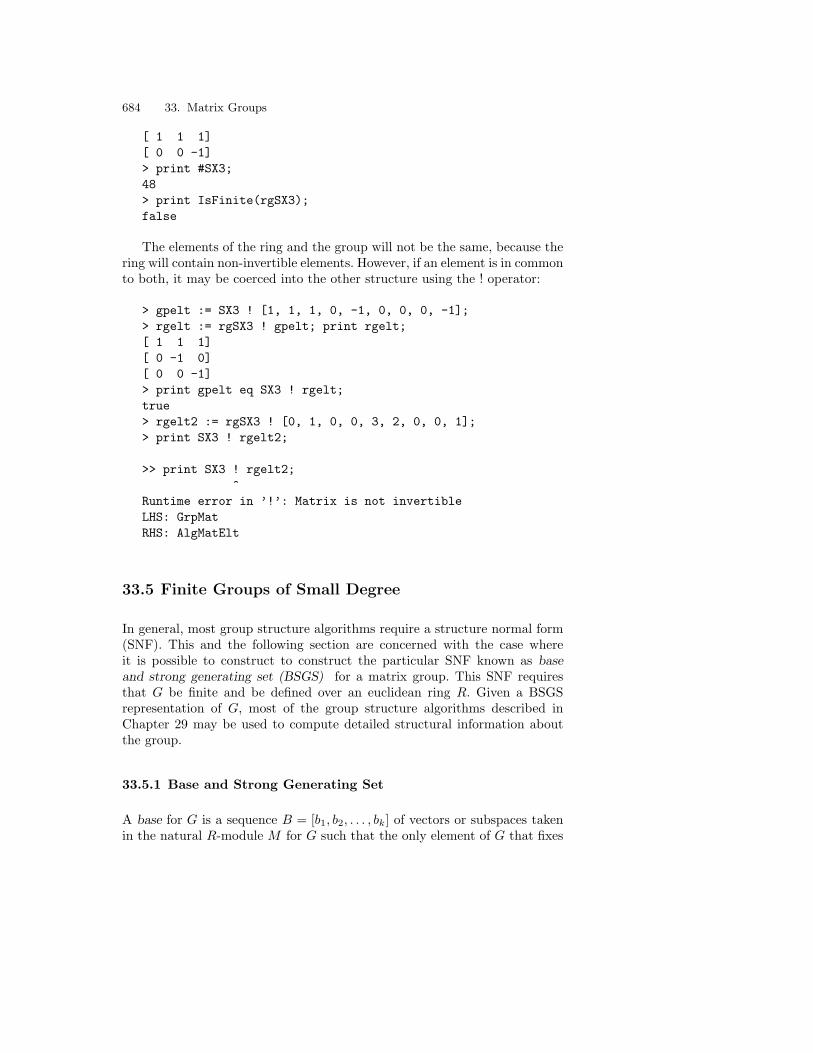
684 33. Matrix Groups
[ 1 1 1][ 0 0 -1]> print #SX3;48> print IsFinite(rgSX3);false
The elements of the ring and the group will not be the same, because thering will contain non-invertible elements. However, if an element is in commonto both, it may be coerced into the other structure using the ! operator:
> gpelt := SX3 ! [1, 1, 1, 0, -1, 0, 0, 0, -1];> rgelt := rgSX3 ! gpelt; print rgelt;[ 1 1 1][ 0 -1 0][ 0 0 -1]> print gpelt eq SX3 ! rgelt;true> rgelt2 := rgSX3 ! [0, 1, 0, 0, 3, 2, 0, 0, 1];> print SX3 ! rgelt2;
>> print SX3 ! rgelt2;^
Runtime error in ’!’: Matrix is not invertibleLHS: GrpMatRHS: AlgMatElt
33.5 Finite Groups of Small Degree
In general, most group structure algorithms require a structure normal form(SNF). This and the following section are concerned with the case whereit is possible to construct to construct the particular SNF known as baseand strong generating set (BSGS) for a matrix group. This SNF requiresthat G be finite and be defined over an euclidean ring R. Given a BSGSrepresentation of G, most of the group structure algorithms described inChapter 29 may be used to compute detailed structural information aboutthe group.
33.5.1 Base and Strong Generating Set
A base for G is a sequence B = [b1, b2, . . . , bk] of vectors or subspaces takenin the natural R-module M for G such that the only element of G that fixes

33.5 Finite Groups of Small Degree 685
B pointwise is the identity. Set G(0) = G, and G(i) = Gb1,...,bi−1 for i ≥ 1.The subgroup chain giving the required representation of G consists of thestabilizers
G = G(0) ≥ G(1) ≥ G(1) ≥ . . . ≥ G(k) = 1.
The construction of a BSGS depends upon being able to choose an objectbi (vector or subspace) in the natural module M such that the orbit ∆i ofbi under G(i−1) is not excessively long, i.e. generally having length less thana million. Usually, once suitable choices have been made for the first andsecond base points, b1 and b2, then it is easy to find suitable candidates forthe remainder.
A BSGS for a matrix group is constructed by some version of the Schreier-Sims algorithm. Any calculation requiring a BSGS will automatically triggeran attempt to construct it, unless one is already known. As the degree of thegroup increases, the cost of computing a BSGS quickly becomes excessive.Thus, in some circumstances, it is better for the user to control the manner inwhich a BSGS is constructed. The standard method available for constructinga BSGS for a matrix group is the Todd-Coxeter Schreier algorithm which maybe invoked by means of the procedure ToddCoxeterSchreier(G).
The random Schreier algorithm attempts to construct a BSGS by meansof a randomized procedure. Without additional information, this version ofthe algorithm cannot prove that it has found a correct BSGS for G. Thealgorithm terminates when m randomly chosen elements of G have failed toenlarge the group defined by the current BSGS. The random Schreier maybe invoked by the procedure RandomSchreier(G). The default value ofm (40) may be changed by the assigning the desired value to the parame-ter Run. The random Schreier algorithm provides a cheap way of obtaininga lower bound on the order of G. Consider the group SL(5, 8). The proce-dure RandomSchreier will be used to find a probable BSGS, and there-fore a probable value for the order of G. The user can obtain some idea ofthe progress of the algorithm by setting a verbose flag, using the procedureSetVerbose:
> SetVerbose("RandomSchreier", 1);> G := SL(5, 8);> time RandomSchreier(G);New strong generator after 1.040 seconds and 11 failuresCurrent ’order’ is 2^3 * 3^2 * 5 * 13 * 31 * 151New strong generator after 1.670 seconds and 1 failuresCurrent ’order’ is 2^4 * 3^2 * 5 * 7 * 13 * 31 * 151New strong generator after 3.350 seconds and 6 failuresCurrent ’order’ is 2^9 * 3^2 * 5 * 13 * 31 * 73 * 151New strong generator after 4.550 seconds and 1 failuresCurrent ’order’ is 2^9 * 3^4 * 5 * 7 * 13 * 31 * 73 * 151New strong generator after 6.900 seconds and 0 failuresCurrent ’order’ is 2^18 * 3^4 * 5 * 13 * 31 * 73 * 151

686 33. Matrix Groups
New strong generator after 8.820 seconds and 3 failuresCurrent ’order’ is 2^19 * 3^4 * 5 * 7 * 13 * 31 * 73 * 151New strong generator after 11.571 seconds and 2 failuresCurrent ’order’ is 2^30 * 3^4 * 5 * 13 * 31 * 73 * 151New strong generator after 14.041 seconds and 0 failuresCurrent ’order’ is 2^30 * 3^4 * 5 * 7 * 13 * 31 * 73 * 151New strong generator after 16.621 seconds and 0 failuresCurrent ’order’ is 2^30 * 3^4 * 5 * 7^2 * 13 * 31 * 73 * 151New strong generator after 19.211 seconds and 1 failuresCurrent ’order’ is 2^30 * 3^4 * 5 * 7^3 * 13 * 31 * 73 * 151New strong generator after 22.312 seconds and 0 failuresCurrent ’order’ is 2^30 * 3^4 * 5 * 7^4 * 13 * 31 * 73 * 151Random Schreier finished in 23.122 seconds76 random generators were testedTime: 24.372> print HasAttribute(G, "Order");true 4638226007491010887680
The Order attribute is now set, with the value 4638 226 007 491 010 887 680,so this is the probable order of G. However, if the function Order is nowinvoked then Magma will try to verify this value, effectively by callingVerify(G) to engage the Todd-Coxeter Schreier method.
If the user knows the order n of G, it should be communicated to Magmausing the statement AssertAttribute(G, "Order", n). Alternatively, if theorder n is given as a factorization sequence Q, then Q may be supplied in placeof n as the third argument. When the order of G is stored, the random Schreieralgorithm will continue until a BSGS is constructed for a group of order n.Thus, the result is guaranteed to be correct in this situation. This is the fastestknown way of computing a BSGS. If the order of G has not been supplied butthe user believes that the BSGS is correct, this information can be assertedby means of the procedure AssertAttribute(G, "IsVerified", true). Inthis situation, if the BSGS is not correct, results depending upon it mat beincorrect or Magma may crash in an unexpected way during subsequentcomputations involving G.
A probable BSGS constructed by the RandomSchreier may be checkedusing the function Verify(G). If the BSGS is incomplete, Verify will causeit to be completed by applying the Todd-Coxeter Schreier algorithm. Con-sequently, the use of RandomSchreier followed by Verify is generally nofaster than having called ToddCoxeterSchreier(G) at the outset.
33.6 The Natural R-module
Every matrix group G of degree n over a ring R has a natural action on itsunderlying R-module R(n). This section is concerned with this action.

33.6 The Natural R-module 687
33.6.1 Action on the Natural R-module
The function RSpace(G) returns the natural R-module for a subgroup ofGL(n,R). Note that it returns an R-module, not an R[G]-module. If R isa field, the function will return a vector space. For example, consider theMathieu group M11 of order 7920 in a 5-dimensional representation over thefield K = GF(3).
> K := GF(3);> G := MatrixGroup< 5, K |> [ 2,1,2,1,2, 2,0,0,0,2, 0,2,0,0,0,> 0,1,2,0,1, 1,0,2,2,1 ],> [ 2,1,0,2,1, 1,2,0,2,2, 1,1,2,1,1,> 0,2,0,1,1, 1,1,2,2,2 ] >;> print G;MatrixGroup(5, GF(3))Generators:
[2 1 2 1 2][2 0 0 0 2][0 2 0 0 0][0 1 2 0 1][1 0 2 2 1]
[2 1 0 2 1][1 2 0 2 2][1 1 2 1 1][0 2 0 1 1][1 1 2 2 2]
> V := RSpace(G);> print V;Full Vector space of degree 5 over GF(3)
A matrix group acts on its natural module by multiplication on the right.Either the multiplication operator (∗) or the exponentiation operator (^) maybe used to compute images with respect to this action.
> v := V![2, 0, 0, 1, 2];> print v ^ (G.1);(0 0 1 0 1)> print v * (G.1);(0 0 1 0 1)
The same operators may be used to calculate the image of a set, sequence orsubspace. For instance:

688 33. Matrix Groups
> print sub<V|v, V.4> ^ (G.1);Vector space of degree 5, dimension 2 over GF(3)Echelonized basis:(0 1 0 0 2)(0 0 1 0 1)
> H := sub< G | G.1^2 * G.2 >;> print Order(H);6> print v ^ H;
(1 2 0 2 0),(1 0 0 0 2),(2 0 0 1 2)
The reader may wish to compare this section with the permutation groupoperations in Section 32.6.
33.6.2 Orbits and Stabilizers
For the remainder of this section it will be assumed that the matrix groupG is defined over an euclidean ring R. Let M be the natural R-module forthe group G. The function Orbit(G,T ) or T^G computes the orbit of theobject T under the action of G, where T may be either a vector of M , aset of vectors, a sequence of vectors or a subspace of M . Note that if theorbit of T is infinite, the function will not return. An alternative function,OrbitBounded(G,T, b) allows the user to specify a limit b on the size ofthe orbit constructed. If the orbit of T under G has length less than or equalto b, the function returns true and the orbit. Otherwise, it simply returnsfalse.
> v := V![2, 0, 0, 1, 2];> w := V![0, 2, 1, 1, 2];> print #Orbit(G, v);22> print #Orbit(G, w);220> print #Orbit(G, v, w);1980> print #Orbit(G, [v, w]);1980> print #Orbit(G, sub< M | v, w >);330

33.6 The Natural R-module 689
If S is a set whose elements are either vectors, sets of vectors, sequences ofvectors, subspaces, sets of subspaces or sequences of subspaces, the functionOrbitClosure(G,S) constructs the smallest G-invariant subset that con-tains S. In other words, OrbitClosure returns the union of orbits of theelements of S.
In the case in which M is both finite and relatively small, the functionOrbits(G) may be used to partition its vectors into orbits, while the func-tion LineOrbits(G) will compute the orbits of G in its action on the one-dimensional subspaces of M :
> orbs := Orbits(G);> print [ #orb : orb in orbs ]; // sum of them = size of V[ 1, 220, 22 ]> lorbs := LineOrbits(G);> print [ #orb : orb in lorbs ];[ 110, 11 ]
The function Stabilizer(G,T ) constructs the stabilizer of the object Tunder the action of G, where T may be either a vector of M , a sequence ofvectors or a subspace of M .
> Gv := Stabilizer(G, v);> print #Gv;360Sw := Stabilizer(G, w);> print #Sw;36> Svw := Stabilizer(G, [v, w] );> print #Svw;4> Ss := Stabilizer(G, sub< V | v,w >);> print Ss;MatrixGroup(5, GF(3)) of order 24 = 2^3 * 3Generators:
[2 1 2 2 1][2 0 2 1 1][1 1 1 2 0][2 2 1 2 2][1 1 2 2 2]
[0 0 0 2 2][0 1 0 0 0][1 2 2 2 0][2 0 0 0 2]

690 33. Matrix Groups
[0 0 0 0 1]
[0 2 1 2 1][0 1 0 0 0][0 0 1 0 0][0 1 0 2 0][1 2 2 2 0]
33.6.3 The Induced Action on an Orbit
Assume that G is a finite group with natural module M for which it is possibleto construct a SNF. Let T be, as usual, a vector, set of vectors, sequence ofvectors or a subspace of M . Let U be the smallest G-invariant set containingT . Then the natural action of G on the elements of U induces a permutationrepresentation φ of G: φ : G → L. Functions to compute this action or merelyits image or kernel are listed in Table 33.5.
Table 33.5. The orbits action homomorphism
Magma Meaning
OrbitAction(G, S) Constructs permutation representation L of G corre-sponding to the action of G on the orbit closure of theset S. Returns (i) natural homomorphism φ : G → L,(ii) induced group L, (iii) kernel of the action
OrbitImage(G, S) Induced group L which is the image of the abovehomomorphism
OrbitKernel(G, S) Kernel of the above homomorphism
OrbitActionBounded(G, S, b) Constructs permutation representation L of G corre-sponding to the action of G on the orbit closure C ofthe set S provided that the size of C does not exceedthe positive integer b. Returns (i) true is successfultogether with (ii) natural homomorphism φ : G → L,(iii) induced group L, (iv) kernel of the action. If |C|exceeds b, the value false is returned
OrbitImageBounded(G, S, b) Induced group L which is the image of the abovehomomorphism
OrbitKernelBounded(G, S, b) Kernel of the above homomorphism
The subgroup G of GL(3, 7) generated by the matrices
1 0 01 6 43 0 6
and
3 0 03 4 46 4 0

33.6 The Natural R-module 691
has order 98 784. The OrbitAction function will be used to find the compo-sition factors of G by reducing to the computation of factors in permutationgroups.
> K := GF(7);> G := MatrixGroup< 3, K | [ 1,0,0, 1,6,4, 3,0,6 ],> [ 3,0,0, 3,4,4, 6,4,0 ] >;> print OrderG);98784> M := RSpace(G);> v := M![1,0,0];> O := Orbit(G, v);> print #O;6> phi, Im, Ker := OrbitAction(G, O);> print Im;Permutation group Im acting on a set of cardinality 6Order = 6 = 2 * 3
(1, 6)(2, 5)(3, 4)(1, 3, 2, 6, 4, 5)
> print Ker;MatrixGroup(3, GF(7)) of order 16464 = 2^4 * 3 * 7^3Generators:
[1 0 0][1 6 4][3 0 6]
[1 0 0][5 1 1][5 3 4]
> U := sub< M | [0,1,0] >;> P := Orbit(Ker, U);> print #P;56> phi1, Im1, Ker1 := OrbitAction(Ker, U);> print Order(Im1);16464> print Order(Ker1);1> print CompositionFactors(Im1);
G| A(1, 7) = L(2, 7)*| Cyclic(2)*

692 33. Matrix Groups
| Cyclic(7)*| Cyclic(7)1
33.7 The Natural K[G]-module
Let G be a matrix group defined over a field K and let M be the naturalK[G]-module for G. This section is concerned with the action of G on propersubmodules and quotient modules of M .
33.8 Submodules
A matrix group G is said to act irreducibly on its natural module M , if M hasno (G-invariant) submodules. The function IsIrreducible(G) returns trueif G acts irreducibly on M . If M is reducible under the action of G, thenIsIrreducible returns false together with a proper submodule of M .
> K<w> := GF(4);> G := MatrixGroup< 6, K |> [ 1,0,w,0,0,0, 0,0,0,0,w^2,0, w^2,0,w^2,0,0,0,> 0,0,0,w^2,0,1, 0,w,0,0,0,0, 0,0,0,w,0,w ],> [ 1,0,1,0,0,0, 0,w,0,0,0,0, 0,0,1,0,0,0,> 0,0,0,1,0,1, 0,w^2,0,0,w^2,0, 0,0,0,0,0,1 ] >;> print G;MatrixGroup(6, GF(2^2))Generators:
[ 1 0 w 0 0 0][ 0 0 0 0 w^2 0][w^2 0 w^2 0 0 0][ 0 0 0 w^2 0 1][ 0 w 0 0 0 0][ 0 0 0 w 0 w]
[ 1 0 1 0 0 0][ 0 w 0 0 0 0][ 0 0 1 0 0 0][ 0 0 0 1 0 1][ 0 w^2 0 0 w^2 0][ 0 0 0 0 0 1]

33.8 Submodules 693
> b, N := IsIrreducible(G);> print b;false> print N:Maximal;GModule N of dimension 2 over GF(2^2)Generators of acting algebra:
[w^2 1][ w w]
[ 1 1][ 0 1]> G1 := QuotientModuleImage(G, N);> print G1;MatrixGroup(4, GF(2^2))Generators:
[ 1 0 w 0][ 0 0 0 w^2][w^2 0 w^2 0][ 0 w 0 0]
[ 1 0 1 0][ 0 w 0 0][ 0 0 1 0][ 0 w^2 0 w^2]
> print #G2;10800> G2 := SubmoduleImage(G, N);> print G2;MatrixGroup(2, GF(2^2))Generators:
[w^2 1][ w w]
[ 1 1][ 0 1]
> print #G1;180> b, U := IsIrreducible(G1);> b;false> print U;GModule U of dimension 2 over GF(2^2)> b, V := IsIrreducible(G2);

694 33. Matrix Groups
> print b;true> G11 := SubmoduleImage(G1, U);> #G11;180> G12 := QuotientModuleImage(G1, U);> print #G12;60> print IsIrreducible(G11);true> print IsIrreducible(G12);true
The function GModule(G) creates the natural K[G]-module M for thegroup G. Now the functions described in Chapter 29 for computing withK[G]-modules may be applied to analyze the structure of M .
33.9 Actions Induced from a Submodule
33.10 Matrix Groups of Large Degree over a Finite Field
The facilities described earlier in this chapter for computing structural infor-mation for finite matrix groups, depend upon being able to construct a baseand strong generating set. However, there are many examples of groups ofmoderately small degree defined over finite fields where this is not practical.A major project, involving a large group of mathematicians and directed byCharles Leedham-Green, is concerned with the development of an alterna-tive approach to investigating matrix groups defined over finite fields whichare outside the range for which BSGS techniques apply. The basis of this ap-proach is the Aschbacher classification of the maximal subgroups of GL(n, q).At the time of writing much work remains to be done so that the functionspresented in this section represent an early stage of the project. Interestedreaders should consult a current Handbook for up-to-date details.
33.10.1 Recognizing Classical Groups
Let G be a subgroup of GL(n, q). The functions in Table 33.6 employ LasVegas algorithms to determine whether, modulo scalars, G lies between a clas-sical simple group and its automorphism group. The functions whose namesend with the word Type do precisely this while the remaining functions ei-ther test whether G is a specific group or contains a specific classical group.

33.10 Matrix Groups of Large Degree over a Finite Field 695
Table 33.6. Las Vegas recognition of classical groups
Magma Meaning
IsClassicalGroup(G) true if S ≤ G ≤ Aut(S), where S is a classicalgroup. (See text for details)
IsLinearGroup(G) true if SL(d, q) ≤ G ≤ GL(d, q)
IsSpecialLinearGroup(G) true if G is the special linear group SL(n, q)
IsSymplecticType(G) true if G preserves a symplectic form up to scalarmultiplication by a constant. In this case the formis also returned
IsSymplecticGroup(G) true if G is the symplectic group Sp(n, q)
IsOrthogonalType(G) true if G preserves an orthogonal form (quadraticform for even characteristic) up to scalar multipli-cation by a constant. In this case the form is alsoreturned
IsOrthogonalGroup(G) true if either SO+(n, q) ≤ G ≤ GO+(n, q) orSO−(n, q) ≤ G ≤ GO−(n, q) for n even, orSO(n, q) ≤ G ≤ GO(n, q) for n odd
IsSpecialOrthogonalGroup(G) true if G is either of the special orthogonal groupsSO+(n, q) or SO−(n, q) for n even, or SO(n, q) forn odd.
IsUnitaryType(G) true if G preserves a unitary form up to scalarmultiplication by a constant. In this case the formis also returned
IsUnitaryGroup(G) true if SU(n, q) ≤ G ≤ GU(n, q)
IsSpecialUnitaryGroup(G) true if G is the special unitary group SU(n, q)
If any of these functions returns true, the answer is guaranteed to be correct.However, if the value false is returned, the most that can be asserted is thatG is probably not the group in question.
The function IsClassicalGroup combines the effect of several of thefunctions listed in Table 33.6. If it successfully recognizes G as lying betweensome classical simple group S and its automorphism group, it returns truetogether with a string naming the family to which S belongs and in the caseof the symplectic, orthogonal and unitary cases, the form that is fixed by thegroup.
33.10.2 The Aschbacher Families
According to a theorem of Aschbacher, (M. Aschbacher, 1On the maximalsubgroups of the finite classical groups, Invent. Math. 76 (1984) 469-514.),a matrix group G acting on the finite dimensional KG-module V over a1 [1]

696 33. Matrix Groups
finite field K satisfies at least one of the following conditions (which we havesimplified slightly for brevity):
– (i) G acts reducibly on V ;
– (ii) G acts semilinearly over an extension field of K;
– (iii) G acts imprimitively on V ;
– (iv) G preserves a nontrivial tensor-product decomposition of V ;
– (v) G has a normal subgroup N , acting absolutely irreducibly on V , whichis an extra-special p-group or 2-group of symplectic type;
– (vi) G preserves a nontrivial symmetric tensor-product decomposition ofV ;
– (vii) G acts (modulo scalars) linearly over a proper subfield of K;
– (viii) G contains the special linear group, or one of the classical groups inits natural action over K;
– (ix) G is almost simple.
The philosophy behind the functions described here is to attempt to de-cide that G lies in at least one of the above categories, and to calculate theassociated isomorphism or decomposition explicitly. Groups in Category (i)can be recognised easily by means of the Meataxe functions described inthe chapter on R-modules. Considerable progress has also been made in therecognition of groups in Category (viii).
Groups which acts irreducibly but not absolutely irreducibly on V falltheoretically into Category (ii), and furthermore act linearly over an extensionfield of K. In fact, absolute irreducibility can be tested using the built-inMagma functions and, by redefining their field to be an extension field Lof K and reducing, they can be rewritten as absolutely irreducible groups ofsmaller dimension, but over L instead of K. We can therefore concentrate onabsolutely irreducible matrix groups.
33.11 Invariants for Finite Groups
In this section G is assumed to be a finite matrix group defined over a fieldK or a permutation group. Magma incorporates powerful new algorithmsfor computing both ordinary and modular invariants of such finite groups.
Table 33.7 lists the functions in Magma for computing within invariantrings. The functions taking a group G can be supplied a matrix group for G,

33.11 Invariants for Finite Groups 697
or a permutation group G followed by (i.e. as the immediately next argument)the desired coefficient field. Using a permutation group speeds up enormouslythe computation of invariants of a fixed degree since only orbits of monomialsunder the group action need be computed.
Table 33.7. Invariant Theory Constructions
Magma Meaning
IsInvariant(f, g) True iff polynomial f is an invariant ofgroup element g
IsInvariant(f, G) True iff polynomial f is an invariant ofgroup G
MolienSeries(G) The Molien series of group G, as a rationalfunction
MonomialsOfDegree(P, d) A indexed set containing all monomials ofdegree d from polynomial ring P
InvariantsOfDegree(G, d) A K-basis of the invariants of degree d ofG
InvariantsOfDegree(G, d, k) k linearly independent invariants of degreed of G
PrimaryInvariants(G) A sequence of primary invariants of G
SecondaryInvariants(G) A sequence of secondary invariants of G
InvariantRing(G) Invariant ring of G
In the first example, primary and secondary invariants for a 2-dimensionalcomplex representation of the cyclic group G of order 4 will be computed.Firstly, the Molien series of G is constructed to give information about thepossible degrees of the primary invariants. The function PrimaryInvariantsproduces primary invariants of G of degrees 2 and 4. Then the functionSecondaryInvariants produces two secondary invariants of degrees 0 and4 with respect to these primary invariants. Note that previous methods forcomputing primary invariants would usually produce the two invariants x14
and x24 of degrees 4 and 4, leading to the secondary invariants 1, x1∗x2, x12∗x22, x13 ∗ x23 of degrees 0, 2, 4, 6.
> K<i> := CyclotomicField(4);> G := MatrixGroup<2, K | [i,0, 0,-i]>;> M<t> := MolienSeries(G);> print M;(t^4 + 1)/(t^6 - t^4 - t^2 + 1)> P<t> := PowerSeriesRing(IntegerRing());> print P ! M;1 + t^2 + 3*t^4 + 3*t^6 + 5*t^8 + 5*t^10 + 7*t^12 +

698 33. Matrix Groups
7*t^14 + 9*t^16 + 9*t^18 + O(t^20)> print PrimaryInvariants(G);[
x1*x2,x1^4 + x2^4
]> print SecondaryInvariants(G);[
1,x1^4
]
In this second example, we compute primary and secondary invariants forthe regular permutation representation of the cyclic group G of order 4 overthe finite field of size 2. Since the characteristic of the field divides the order ofthe group, we are in the modular case, and there is no Molien series. There areprimary invariants of degrees 1, 2, 2, 4, and secondary invariants of degrees0, 3, 3, 4, 5 with respect to these primary invariants. The whole process takesa small fraction of a second even though the computation of the secondaryinvariants involves a non-trivial Grobner basis elimination computation ona module of degree 16—the computation is dramatically improved by usingthe Hilbert-driven Buchberger algorithm.
> K := GF(2);> G := CyclicGroup(4);> time PrimaryInvariants(G, K);[
x1 + x2 + x3 + x4,x1*x2 + x1*x4 + x2*x3 + x3*x4,x1*x3 + x2*x4,x1*x2*x3*x4
]Time: 0.019> time SecondaryInvariants(G, K);[
1,x1*x2*x3 + x1*x2*x4 + x1*x3*x4 + x2*x3*x4,x1^2*x3 + x1^2*x4 + x1*x2^2 + x1*x3^2 + x2^2*x4 +
x2*x3^2 + x2*x4^2 + x3*x4^2,x1^2*x3^2 + x1^2*x3*x4 + x1*x2^2*x4 + x1*x2*x3^2 +
x2^2*x4^2 + x2*x3*x4^2,x1^3*x3*x4 + x1^2*x2^2*x3 + x1^2*x2^2*x4 +
x1^2*x2*x3^2 + x1^2*x2*x3*x4 + x1^2*x2*x4^2 +x1^2*x3^2*x4 + x1^2*x3*x4^2 + x1*x2^3*x4 +x1*x2^2*x3^2 + x1*x2^2*x3*x4 + x1*x2^2*x4^2 +

33.11 Invariants for Finite Groups 699
x1*x2*x3^3 + x1*x2*x3^2*x4 + x1*x2*x3*x4^2 +x1*x3^2*x4^2 + x2^2*x3^2*x4 + x2^2*x3*x4^2 +x2*x3^2*x4^2 + x2*x3*x4^3
]Time: 0.060


Part VIII
Algebraic Geometry


34. Elliptic Curves
This chapter contains descriptions for functions pertaining to arithmeticwith elliptic curves. The category to which elliptic curves belong is calledCurveEll; points on curves are of type CurveEllPt; and there is also aspecial category for Kodaira symbols SymKod.
This module is currently under construction; the main functions thatare present deal with elementary arithmetic over fields, and with more so-phisticated questions over the rational field. The latter include functions forminimal models, local information (Tate’s algorithm), and the computationof the Mordell-Weil group. These facilities are based on implementations byJohn Cremona. Refer to his book [Cre92] for details.
34.1 Some Algebraic Geometry
It is not easy to define elliptic curves informally without some knowledge ofalgebraic geometry. One formal definition is that an elliptic curve over a fieldis a plane, non-singular cubic curve, of genus 1, with a rational point. Most ofthe terms in this definition can be made intuitively clear. A plane curve overa field F is given by a polynomial equation P (X,Y ) = 0 with coefficients inthe field; a cubic curve is a curve for which the polynomial P has degree three,and a rational point means, in this context, that there exists a point (x, y)with x, y ∈ F such that P (x, y) = 0. It is somewhat more difficult to explainwhat genus 1 means. Moreover, in algebraic geometry points are allowed to beat infinity, and therefore it is necessary to cater for that by using projectivecoordinates (x : y : z) rather than affine coordinates (x, y) for the plane. Aprojective point in the plane over the field F is not merely a triple (x, y, z) ofelements of F , but it is an equivalence class of such triples, where two triples(x, y, z) and (x′, y′z′) are equivalent if and only if there exists a non-zeroelement u ∈ F such that ux = x′, uy = y′, and uz = z′. The triple (0, 0, 0)is not a valid projective point. The way to think of these projective pointsis that there are those corresponding to ‘ordinary’ points, namely those withz 6= 0, and ‘extraordinary’ points (‘at infinity’), namely those with z = 0. Forthe ordinary points the usual choice of representative has z = 1, which gets

704 34. Elliptic Curves
back to pairs (x, y) distinguishing them. At infinity, there are those pointsfor which y 6= 0, with representatives (x, 1, 0), and those for which y = 0 aswell, represented by (1, 0, 0). (Perhaps it is clear, from all this dividing out bynon-zero elements, how convenient it is to assume the coordinates are froma field!)
A plane cubic curve over F in projective coordinates is given by a ho-mogeneous cubic polynomial equation C(X, Y, Z) = 0 with coefficients in F ;homogeneous cubic means that every term has total degree 3 (in the variablesX, Y, Z). Non-singular now just means that at no point of F are the threepartial derivatives of C (with respect to X, Y , Z) zero simultaneously.
Algebraic geometers like to classify objects up to ‘birational equivalence’;that is, to consider things equal if there exists a 1–1 transformation betweenthem with maps defined by quotients of polynomials with coefficients in thefield F . It turns out that non-singular plane cubic curves of genus 1 with arational point have a canonical form. That is, there is a birational transfor-mation putting such a curve into that standard form. The canonical form isusually referred to as the Weierstrass form, and it looks like this:
Y 2Z = X3 + aXZ2 + bZ3.
So any elliptic curve E can be brought into Weierstrass form by a changeof projective variables; from now on, elliptic curves will be defined for us bysuch a Weierstrass form. Moreover, the ‘distinguished’ rational point on suchan elliptic curve will always be O = (0 : 1 : 0). This is only strictly true if thecharacteristic of the field is not 2 or 3; in those cases the canonical form isslightly more complicated (because it is impossible to ‘complete the square’,or cube, in the field):
Y 2Z + a1XY Z + a3Y Z2 = X3 + a2X2Z + a4XZ2 + a6Z
3,
which is called the extended Weierstrass form.
The most important fact for computational purposes is the following: thecollection of all points (x : y : z) in the projective plane over F (which isnon-empty since it contains O) forms an abelian group (indicated by E(F ))of points on the curve. Moreover, the ‘addition’ in this group is very simple,and can be given explicitly in terms of the coefficients of the points; the pointO is the zero element of the group, and the inverse of a point (x : y : z) issimply (x : −y : z). Geometrically, the group law is given by a tangent andchord construction.
The most interesting cases for us are those where the field of definitionis either a finite field, or the field of rational numbers. In the first case, thenumber of points over a finite field must be finite. In the second case this isnot true, but the groups are not completely arbitrary.

34.2 Elliptic Curves over Arbitrary Fields 705
34.2 Elliptic Curves over Arbitrary Fields
34.2.1 Creation and Basic Quantities
An elliptic curve is defined by giving a sequence of its Weierstrass coefficients;these coefficients must be elements from a field, which will be the field of def-inition of the curve, or from ZZ, in which case the field of definition will beQ. The sequence of Weierstrass coefficients may have length 2 or 5, corre-sponding to the normal and extended Weierstrass forms respectively. Thesecoefficients must define a non-singular curve; singularity gives an error. Thefunction IsEllipticCurve can be used to determine if the coefficients definea non-singular curve; if so, this curve is returned as the second value.
> F<f> := FiniteField(25);> E := EllipticCurve( [f^2, -1] );
>> E := EllipticCurve( [f^2, -1] );^
Runtime error in ’EllipticCurve’: Curve is not non-singular> print IsEllipticCurve( [f^2, -1] );false> E := EllipticCurve( [f, -1] );> ok, E2 := IsEllipticCurve( [f, -1] );> print ok;true> print E2 eq E;true> print E;Elliptic Curve defined by y^2 = x^3 + f*x + 4 over GF(5^2)
Now E is an elliptic curve over F = GF(25). Table 34.1 lists the functionsfor retrieving various quantities associated with a curve. Note that the dis-criminant is always non-zero for a valid (i.e. non-singular) elliptic curve.
34.2.2 Points on Elliptic Curves
Points on a curve can be created either by using an element constructor orby coercing a sequence of coefficients; in both cases 2 or 3 coefficients mustbe specified; in the former case z = 1 will be assumed. The point will benormalized if necessary:
> P := elt< E | f^2, f^5 >;> Q := E ! [ 4, 2*f^2, 2 ];

706 34. Elliptic Curves
Table 34.1. Basic quantities associated with an elliptic curve
Magma Meaning
CoefficientRing(E),BaseRing(E)
The field of definition of the elliptic curve E
aInvariants(E),Coefficients(E)
The sequence [a1, a2, a3, a4, a6] of extended Weier-strass coefficients of E
bInvariants(E) The sequence [b2, b4, b6, b8] of b-invariants of E
cInvariants(E) The sequence [c4, c6] of c-invariants of E
Discriminant(E) The discriminant of E
jInvariant(E) The j-invariant of E
> O := E ! 0;> print P, Q, O;(f^2, f^5, 1) (2, f^2, 1) (0, 1, 0)
The special point O can be defined either using Identity, or by coercing 0as in the example.
The symbol + is used for the group law on the curve.
> R := P+Q;> print R, R-P eq Q, P+O, O+P eq P, IsIdentity(Q);(f^10, f^8, 1) true (f^2, f^5, 1) true false
Let us simply enumerate all points in E(F ). For every possible x we determinewhether x3 + fx + 4 is a square in the field; if so we take its square root y,and include (x : y : 1). Afterwards we also include all negates (x : −y : 1),and then the identity O (which is its own negative, of course).
> Pts := E ! [x, Sqrt(P)] : x in F | IsSquare(P)> where P is x^3+f*x+4 ;> Pts join:= -P : P in Pts ;> Pts join:= O ;> print #Pts;28
So our curve has 28 points defined over F . Let us print the order of allelements.
> ord := function(P)> Q := P;> n := 1;> O := Identity(Parent(P));

34.2 Elliptic Curves over Arbitrary Fields 707
> while Q ne O do> Q := P+Q;> n +:= 1;> end while;> return n;> end function;> for P in Pts do> print P, ord(P);> end for;(f^15, 4, 1) 14(f^20, f^14, 1) 28(2, f^14, 1) 7(f^15, 1, 1) 14(f^4, f^5, 1) 28(f^5, f^13, 1) 28(f^10, f^8, 1) 14(f^2, f^17, 1) 14(f^5, f, 1) 28(f^7, f^17, 1) 28(f^3, f^15, 1) 7(f, 0, 1) 2(f^3, f^3, 1) 7(f^13, f^21, 1) 28(f^4, f^17, 1) 28(f^11, f^22, 1) 7(0, 2, 1) 28(f^11, f^10, 1) 7(f^20, f^2, 1) 28(f^10, f^20, 1) 14(f^13, f^9, 1) 28(f^21, f^14, 1) 4(f^2, f^5, 1) 14(0, 1, 0) 1(2, f^2, 1) 7(f^7, f^5, 1) 28(f^21, f^2, 1) 4(0, 3, 1) 28>> print 14 * (E ! [0,3,1]);(f, 0, 1)
We see that the points defined over GF(5) do not form a subgroup (becausethe curve is not defined over GF(5)). Finding points over a subfield can bedone with a simple check:

708 34. Elliptic Curves
> print P : P in Pts | P[1] in GF(5) and P[2] in GF(5) ; (0, 2, 1), (0, 3, 1), (0, 1, 0)
but to find points over an extension field requires Lift:
> M<m> := ext< F | 2 >;> Ee := Lift(E, M);> ePts := Ee ! [x, Sqrt(P)] : x in M | IsSquare(P)> where P is x^3+f*x+4 ;> ePts join:= -q : q in Epts ;> ePts join:= Ee ! 0 ;> print #ePts;672> print exists P : P in ePts | ord(P) eq 672 ;false
Observe that the curve defines a non-cyclic group of order 672, which hasE(F ) as a subgroup.
Lift(E,F ) creates a new elliptic curve by coercing the coefficients of thecurve E into the field F . If this results in a singular elliptic curve, then anerror occurs. There is also a three-argument version of Lift, where the thirdargument consists of a map specifying the embedding of the original field ofdefinition into the extension.
34.3 Elliptic Curves over The Rationals
34.3.1 Minimal Models
Two elliptic curves E and E′ are isomorphic if there is a change of coordinatesof a particular form which transforms the equation of E into the equation ofE′. This form is:
x = u2x′ + r
y = u3y′ + su2x′ + t
where r, s, t ∈ K and u ∈ K∗ for some field K. If the coefficients of theequations also lie in K, then the curves are said to be isomorphic over K.For example, the curves y2 = x3 + 17 and y2 = x3 − 17 are isomorphic overC with parameters <r, s, t, u> = <0, 0, 0, i>, but they are not isomorphic overQ.
The effect of such a transformation on the coefficients is:

34.3 Elliptic Curves over The Rationals 709
ua′1 = a1 + 2s
u2a′2 = a2 − sa1 + 3r − s2
u3a′3 = a3 + ra1 + 2t
u4a′4 = a4 − sa3 + 2ra2 − (rs + t)a1 + 3r2 − 2st
u6a′6 = a6 + ra4 − ta3 + r2a2 − rta1 + r3 − t2
whence u12∆′ = ∆ and j′ = j.
It can be seen from the above that suitable choice of u transforms any ellip-tic curve with coefficients in Q into an elliptic curve with coefficients in ZZ. Theresulting discriminant is then an integer. The function IntegralModel(E)returns such a curve:
> EE := EllipticCurve([ 1/2, 1, -1/2, 1/2, 0 ]);> print EE;Elliptic Curve defined by y^2 + 1/2*x*y - 1/2*y = x^3 + x^2+ 1/2*x over Rational Field> print Discriminant(EE);-19/128> IE := IntegralModel(EE);> print IE;Elliptic Curve defined by y^2 + x*y - 4*y = x^3 + 4*x^2 +8*x over Rational Field> print Discriminant(IE);-608
Amongst all such curves over ZZ, those for which |∆| is minimal are calledglobal minimal models. By careful choice of r, s and t a global minimal modelcan be found for which a1, a3 ∈ 0, 1 and a2 ∈ −1, 0, 1; this is called thereduced minimal model (henceforth just minimal model), and it is unique.Comparing minimal models thus gives an easy way to tell if two curves areisomorphic over Q.
The function MinimalModel(E) returns the minimal model M of E, to-gether with the maps E → M and M → E. The function IsIsomorphic(E, F )returns true if the two curves are isomorphic over Q. If so, it returns the map-ping between them as its second return value.
> ME, f1, f2 := MinimalModel(IE);> print ME;Elliptic Curve defined by y^2 + x*y + y = x^3 + x^2 + 1 overRational Field> iso, map := IsIsomorphic(ME, IE);> print iso;true

710 34. Elliptic Curves
> P := elt<ME | 1, -3>;> print map(P);(0, 0, 1)> print f1($1) eq P;true>> E1 := EllipticCurve([ 0, 17 ]);> E2 := EllipticCurve([ 0, -17 ]);> print IsIsomorphic(E1, E2);false
Table 34.2. Functions for models
Magma Meaning
IntegralModel(E) Given an elliptic curve E with coefficients in Q, returnsan isomorphic curve with coefficients in ZZ
MinimalModel(E) Returns (i) the minimal model M of E (ii) the mapE → M (iii) the map M → E
IsIsomorphic(E, F ) true if curves E and F are isomorphic; if so, the mapE → F is returned as the second return value
34.3.2 Local Information
One method of computing the minimal model of a curve is to apply Tate’salgorithm. Given an elliptic curve E and a prime p, Tate’s algorithm producesthe following information: ep, the exponent of p in the discriminant of theminimal model M of E; fp, the exponent of p in the conductor of E; cp, theTamagawa number of E at p; and kp, the Kodaira symbol classifying the typeof reduction of E at p. The algorithm is not described here - see [Cre92] fordetails.
The Tamagawa number cp = [E(Qp) : E0(Qp)], where E0(Qp) is thesubgroup of the group E(Qp) of p-adic points of E whose reduction modulop is non-singular. The Kodaira symbol kp classifies the type of reduction ofE at p as one of: I0 for good reduction - in this case p does not divide thediscriminant of M ; In(n > 0) for bad multiplicative reduction; and one ofI∗n, II, II∗, III, III∗, IV or IV ∗ for bad additive reduction.
Table 34.3 lists the functions available for accessing the local informationof a curve. Note in particular that BadPrimes(E) returns only the primesdividing the discriminant of M , not E; so while it will be safe to lift M intoGF (p), it might not be possible for E:

34.3 Elliptic Curves over The Rationals 711
Table 34.3. Local information
Magma Meaning
BadPrimes(E) Sequence of primes dividing the discriminant ofM , the minimal model of the elliptic curve E
LocalInformation(E, p) Local information tuple <p, ep, fp, cp, kp> of M atthe prime p, where the elements of the tuple areas defined above
LocalInformation(E) Sequence of local information tuples of M foreach bad prime
Conductor(E) Conductor of M
TamagawaNumber(E, p) Tamagawa number of M at p
TamagawaNumbers(E) Sequence of Tamagawa numbers of M for eachbad prime
KodairaSymbol(E, p) Kodaira symbol of M at p
KodairaSymbols(E) Sequence of Kodaira symbols of M for each badprime
> F := EllipticCurve([ 0, 17*5^6 ]);> MF := MinimalModel(F);> print BadPrimes(F);[ 2, 3, 17 ]> print Lift(F, GF(5));
>> print Lift(F, GF(5));^
Runtime error in ’Lift’: Curve is not non-singular> print Lift(MF, GF(5));Elliptic Curve defined by y^2 = x^3 + 2 over GF(5)
Kodaira symbols belong to the special category SymKod. They canbe obtained from the local information of a curve, or created by callingKodairaSymbol(s), where s is one of the strings: "I0"; "In" or "In*"for n > 0; "II"; "III"; "IV"; "II*"; "III*"; or "IV*". The special symbols"In" and "In*" may also be used; they compare equal to the correspondingsymbols with n replaced by any positive integer.
> S := KodairaSymbols(ME);> print S;[ I5, I1 ]> In := KodairaSymbol("In");> print In;In> print S[1] eq In;

712 34. Elliptic Curves
true> print In eq S[2];true> print S[1] eq S[2];false
34.3.3 The Mordell-Weil Group
As mentioned at the beginning of the chapter, the points on an elliptic curveform an abelian group - the Mordell-Weil group. If the curve has coefficientsin Q, then Magma has various functions to calculate information about thisgroup. These are summarized in Table 34.4.
Table 34.4. Group functions
Magma Meaning
TorsionSubgroup(E) (i) abelian group isomorphic to the torsionsubgroup of the group G of rational pointsof E (ii) mapping from this group into E
MordellWeilRank(E),Rank(E)
The computed rank of G
MordellWeilRankBounds(E),RankBounds(E)
The computed lower and upper bounds onthe rank of G
MordellWeilGroup(E) (i) abelian group isomorphic to G (ii) map-ping from this group into E
Generators(E) Sequence [P1, . . . , Pk] of generators of G
Order(P ) The order of P in G; if P is of infinite order,0 is returned
The Mordell-Weil group of a curve over Q is the product of a finite torsionpart T and a free abelian group F of rank r ≥ 0 (F ∼= ZZr). By a theoremof Mazur, the structure of T is either Ck for 1 ≤ k ≤ 10, C12, or C2k × C2
for 1 ≤ k ≤ 4. The function TorsionSubgroup(E) returns an abelian groupisomorphic to T and a mapping from this group into E.
> T,h := TorsionSubgroup(ME);> print T;Abelian Group isomorphic to Z/5Defined on 1 generatorRelations:
5*T.1 = 0> print [ h(t) : t in T ];[ (0, 1, 0), (-1, 1, 1), (1, -3, 1), (1, 1, 1), (-1, -1, 1) ]

34.3 Elliptic Curves over The Rationals 713
> print [ Order(P) : P in $1 ];[ 1, 5, 5, 5, 5 ]> T,h := TorsionSubgroup(E1);> print T;Abelian Group of order 1> print h(T.0);(0, 1, 0)> P := E1 ! [ 2, 5 ];> print Order(P);0> print Order(E1 ! 0);1
Computing the torsion subgroup is fairly straightforward, and, while itmay take some time for large examples, it is the easiest part of the Mordell-Weil group to compute. In contrast, the procedure for calculating the rankof the group (two-descent) is not guaranteed to return the correct result; itwill, however, provide bounds on the rank, and with luck they will be equal.The function MordellWeilRank(E) (or just Rank(E)) returns the lowerbound on the rank; MordellWeilRankBounds(E) (or RankBounds(E))returns both the lower and upper bounds. Note that computing the rank ismuch faster than computing the full group, so these functions should be usedif they suffice.
> E := EllipticCurve([ 0, 0, 1, -7, 6 ]);> time print MordellWeilRank(E);3Time: 0.039> F := EllipticCurve([ 0, 36861504658225, 0,> 1807580157674409809510400, 0 ]);> time print Rank(F);13Time: 131.449> F := EllipticCurve([ -17^2, 0 ]);> print RankBounds(F);0 2
The function MordellWeilGroup(E) returns an abelian group isomor-phic to the Mordell-Weil group and a mapping from this group into E. This isby far the slowest function so far, as it requires searching for the generators.These can be got by using the mapping on the generators of the group, orfrom the intrinsic Generators(E).
> E := EllipticCurve([ 0, 0, 1, -7, 6 ]);

714 34. Elliptic Curves
> time G,h := MordellWeilGroup(E);Time: 0.439> print G;Abelian Group isomorphic to Z + Z + ZDefined on 3 generators (free)> print Generators(E);[ (0, 2, 1), (-1, 3, 1), (-2, 3, 1) ]> print [ h(g) : g in Generators(G) ];[ (-2, 3, 1), (-1, 3, 1), (0, 2, 1) ]
The search for generators requires the concept of the height of a point.If P = (x, y) is a point on E, then the naive height of P is h(P ) = logmax|m|, |n|, where x = m
n . The canonical height h(P ) is the sum of thelocal heights hp(P ) at each prime p and ∞ also. If E has good reduction atp, and p does not divide n, then hp(P ) will be 0. The functions dealing withheights are summarized in Table 34.5.
Table 34.5. Height related functions
Magma Meaning
NaiveHeight(P ) log max|m|, |n|, where mn
is the x-coordinate of P
LocalHeight(P, p) Local height hp(P ) of P at the prime p; to specifyp = ∞ use p = 0
Height(P ) The canonical height h(P ) = Σhp(P ) where the sumis over all primes p and ∞
HeightPairing(P, Q) Height pairing h(P, Q) = 12(h(P + Q)− h(P )− h(Q))
Regulator(E) Regulator of E
> P := Generators(E)[1];> print P;(0, 2, 1)> print NaiveHeight(P);0.E-92
> print LocalHeight(P, 0); /* infinity */0.99090633315308762618> print [ LocalHeight(P, p) : p in BadPrimes(E) ];[ 0.E-92 ]> print &+$1 + $2;0.99090633315308762618> print Height(P);0.99090633315308762618

34.3 Elliptic Curves over The Rationals 715
The process of computing the rank provides the generators of a subgroupof G, the Mordell-Weil group of E. The canonical heights of these pointsprovide a bound on the canonical heights of the generators of G, and a resultof Silverman bounds the difference between a point’s naive and canonicalheights (the function SilvermanBound(E) can be used to get this bound).So we get a bound on the naive heights of the generators of G and simplysearch up to this bound. This bound gets quite large quickly, and for mostcurves this computations is infeasible; if the rank provides sufficient informa-tion it should be used instead.
One other quantity of interest is the regulator of E. If the generators ofthe non-torsion part of G are P1, . . . , Pr, then the regulator of E is R(E) =|det(h(Pi, Pj))| where h(P,Q) = 1
2 (h(P + Q) − h(P ) − h(Q)) is the heightpairing of P and Q. The functions Regulator(E) and HeightPairing(P,Q)can be used to compute these values.
> S := Generators(E);> A := MatrixAlgebra(RealField(), #S);> m := A ! [ HeightPairing(P, Q) : P,Q in S ];> print Determinant(m);0.41714355875838417559> print Regulator(E);0.41714355875838621257


Part IX
Geometric and Combinatorial Structures


35. Enumerative Combinatorics
This chapter presents some of the tools provided by Magma for enumerativecombinatorics. As facilities in this area were still under development at thetime of writing, the user should consult the online help system for an up-to-date list of the facilities.
35.1 Elementary Counting Functions
Table 35.1. Counting functions
Magma Meaning
Factorial(n) n!
NumberOfPermutations(n, k) Number of permutations of n distinct ob-jects, taken k at a time
Binomial(n, k) Binomial coefficient
nk
Multinomial(n, Q) Given integer n and Q = [r1, . . . , rk], where
n = r1 + · · ·+ rk, returns multinomial coef-ficient n!
r1!...rk!
Fibonacci(n) nth Fibonacci number, where F0 = 0, F1 =1 (returns (−1)n−1F−n if n < 0)
StirlingFirst(m, n) Stirling number of the first kind,mn
StirlingSecond(m, n) Stirling number of the second kind,
mn
EulerianNumber(n, r) Number E(n, r) of permutations p of
1, . . . , n having exactly k ascents (i.e.,places where pi < pi+1)
HarmonicNumber(n) nth harmonic number
BernoulliNumber(n) nth Bernoulli number Bn, as a rational
BernoulliApproximation(n) Approximation to Bn, as a finite-precisionfree real
BernoulliPolynomial(n) nth Bernoulli polynomial

720 35. Enumerative Combinatorics
The elementary counting functions of enumerative combinatorics availablein Magma are listed in Table 35.1. Some brief explanation of the less familiarfunctions is given below. The reader is referred to [Rio58] for a full accountof the definition and properties of these functions.
The Stirling number of the first kind,[mn
]or s(m,n), is returned as the
value of StirlingFirst(m,n) and may be interpreted as (−1)m−n times thenumber of ways of arranging m objects into n cycles. The Stirling number ofthe second kind,
mn
or S(m,n), is returned by StirlingSecond(m,n) and
gives the number of ways of partitioning a set of m objects into n non-emptysubsets.
The Bernoulli number Bn, a rational number, is calculated by the func-tion BernoulliNumber(n). A real approximation (calculated to the currentprecision) is given by BernoulliApproximation(n). For example:
> bern50 := BernoulliNumber(50);> print bern50;495057205241079648212477525/66
> bern50app := BernoulliApproximation(50);> print bern50app;7500866746076964366855720.07275390625> print Round(bern50app * 66);495057205241079648212477525
BernoulliPolynomial(n) returns the Bernoulli polynomial Bn(x), whichis defined as Bn(x) =
∑nk=0
(nk
)Bkxn−k, where Bn is the nth Bernoulli num-
ber. For instance:
> p<x> := BernoulliPolynomial(3);> print p;x^3 - 3/2*x^2 + 1/2*x> print &+[Binomial(3,k) * BernoulliNumber(k) * x^(3-k):> k in [0..3]];x^3 - 3/2*x^2 + 1/2*x
35.2 Subsets of a Finite Set
Let S be an enumerated set of cardinality n. The total number of subsetsof S, including the empty set and S itself, is 2n. The function Subsets(S)returns all of these subsets, as an enumerated set of enumerated sets. Forexample:

35.2 Subsets of a Finite Set 721
Table 35.2. Subsets of a finite set
Magma Meaning
Subsets(S) Set of all subsets of S
Subsets(S, k) Set of all k-subsets of S
Multisets(S, k) Set of all k-multisets formed from elements of S
Subsequences(S, k) Set of all k-sequences formed from elements of S
Permutations(S, k) Set of all permutations (as sequences) of elements of S,taken k at a time
Permutations(S) Set of all permutations (as sequences) of elements of S
> print Subsets(1..3);
1 ,, 1, 3 , 2 , 3 , 1, 2, 3 , 2, 3 , 1, 2
The function Subsets(S) should be distinguished from PowerSet(S). Bothfunctions return the same mathematical object, that is, the power set of S.However, Subsets returns the subsets explicitly, whereas PowerSet merelyreturns them as a formal object.
Now, let k be an non-negative integer. A k-subset of S is a subset of Shaving cardinality k, that is, an unordered set of size k whose elements aredistinct elements of S. The function Subsets(S, k) returns all the k-subsetsof S, as an enumerated set of enumerated sets.
Three other concepts resembling the notion of subset-ness may be ob-tained by allowing the subsets to be ordered or to have repeated elements.The function Multisets(S, k) returns an enumerated set containing all themultisets of size k (counting multiplicity) whose elements are in S. Simi-larly, Subsequences(S, k) returns an enumerated set containing all the se-quences (i.e., ordered multisets) of length k whose elements are in S. Finally,Permutations(S, k) returns an enumerated set containing all the distinct-element sequences (i.e., ordered sets) of length k whose elements are in S.There is a special permutation function, Permutations(S), which may beused when k equals the cardinality of S. For all of these functions, if k isgreater than n then an empty set will be returned.
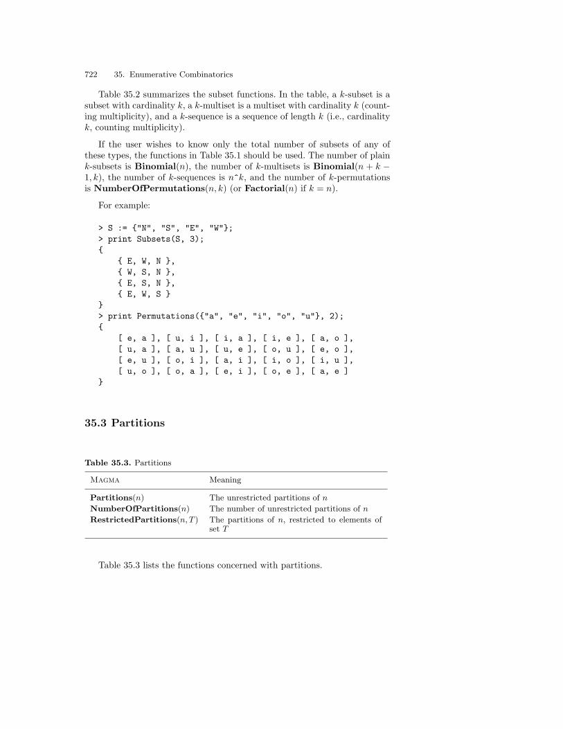
722 35. Enumerative Combinatorics
Table 35.2 summarizes the subset functions. In the table, a k-subset is asubset with cardinality k, a k-multiset is a multiset with cardinality k (count-ing multiplicity), and a k-sequence is a sequence of length k (i.e., cardinalityk, counting multiplicity).
If the user wishes to know only the total number of subsets of any ofthese types, the functions in Table 35.1 should be used. The number of plaink-subsets is Binomial(n), the number of k-multisets is Binomial(n + k −1, k), the number of k-sequences is n^k, and the number of k-permutationsis NumberOfPermutations(n, k) (or Factorial(n) if k = n).
For example:
> S := "N", "S", "E", "W";> print Subsets(S, 3);
E, W, N , W, S, N , E, S, N , E, W, S
> print Permutations("a", "e", "i", "o", "u", 2);
[ e, a ], [ u, i ], [ i, a ], [ i, e ], [ a, o ],[ u, a ], [ a, u ], [ u, e ], [ o, u ], [ e, o ],[ e, u ], [ o, i ], [ a, i ], [ i, o ], [ i, u ],[ u, o ], [ o, a ], [ e, i ], [ o, e ], [ a, e ]
35.3 Partitions
Table 35.3. Partitions
Magma Meaning
Partitions(n) The unrestricted partitions of n
NumberOfPartitions(n) The number of unrestricted partitions of n
RestrictedPartitions(n, T ) The partitions of n, restricted to elements ofset T
Table 35.3 lists the functions concerned with partitions.

35.3 Partitions 723
A partition of an integer n is a representation of it as the sum of positiveintegers, ignoring order. Partitions(n) returns a sequence containing all thepartitions of n, each partition being given as a non-increasing sequence ofpositive integers.
> print Partitions(6);[
[ 6 ],[ 5, 1 ],[ 4, 2 ],[ 4, 1, 1 ],[ 3, 3 ],[ 3, 2, 1 ],[ 3, 1, 1, 1 ],[ 2, 2, 2 ],[ 2, 2, 1, 1 ],[ 2, 1, 1, 1, 1 ],[ 1, 1, 1, 1, 1, 1 ]
]
The function NumberOfPartitions(n), returns the number of these parti-tions:
> print NumberOfPartitions(6), NumberOfPartitions(600);11 458004788008144308553622
The function RestrictedPartitions(n, T ) is similar to Partitions(n),except that it returns only those partitions whose components all lie in theset T of positive integers. For example, in Australia, the coins of value lessthan one dollar have the values 5, 10, 20 and 50 cents. Therefore, the possibleways of giving change for a 50 cent piece are those listed in the output below:
> print RestrictedPartitions(50, 5, 10, 20);[
[ 20, 20, 10 ],[ 20, 20, 5, 5 ],[ 20, 10, 10, 10 ],[ 20, 10, 10, 5, 5 ],[ 20, 10, 5, 5, 5, 5 ],[ 20, 5, 5, 5, 5, 5, 5 ],[ 10, 10, 10, 10, 10 ],[ 10, 10, 10, 10, 5, 5 ],[ 10, 10, 10, 5, 5, 5, 5 ],[ 10, 10, 5, 5, 5, 5, 5, 5 ],[ 10, 5, 5, 5, 5, 5, 5, 5, 5 ],

724 35. Enumerative Combinatorics
[ 5, 5, 5, 5, 5, 5, 5, 5, 5, 5 ]]
35.4 Example: Bell Numbers
The Bell number (or exponential number) Bn may be defined as the numberof partitions of a set of n objects into non-empty subsets. (B0 = 1, sincean empty set may be partitioned uniquely into zero non-empty subsets.)There are several formulae for the Bell numbers (see [LiW92], pp. 105–107and [Ber71], pp. 42–44), some of which will be implemented below. Notethat these formulae/implementations are not equally efficient, but collectivelythe examples demonstrate several techniques in enumerative combinatorics:counting functions, summation of sequences, recursive functions and recursivesequences, generating functions, and approximations to infinite series.
The first formula is based on the Stirling numbers of the second kind:
B0 = 1; Bn =n∑
k=1
n
k
for n ≥ 1.
It is easily implemented by constructing a sequence containing the Stirlingnumbers and then summing its terms using the reduction operator.
> Bell := func< n | n eq 0 select 1 else> &+[ StirlingSecond(n, k) : k in [1..n] ] >;
> time print Bell(3), Bell(15);5 1382958545Time: 0.030> time print Bell(100);47585391276764833658790768841387207826363669686825611466616\334637559114497892442622672724044217756306953557882560751Time: 4.000
The next formula is a recursive summation:
B0 = 1; Bn =n−1∑
k=0
(n− 1
k
)Bk for n ≥ 1.
There are two approaches to the implementation of this formula. The simplestapproach is to implement it as a recursive function.
> Bell := func< n | n eq 0 select 1 else

35.4 Example: Bell Numbers 725
> &+[ Binomial(n-1, k) * $$(k) : k in [0..n-1] ] >;
> time print Bell(3), Bell(15);5 1382958545Time: 16.271
This implementation is inefficient since whenever the function is called for aparticular value of n, every Bk for k ≤ n has to be calculated, and each ofthese calculations, in turn, involves finding all the Bi for i ≤ k. Since the inter-mediate values of Bk are not remembered by the system, they must be com-puted repeatedly. Therefore, it is preferable to calculate and store all Bk fork ≤ N , where N is a pre-determined upper limit, using a recursively-definedsequence. This technique is followed in the code below. Since Magma’s se-quences are indexed beginning at 1, the k = 0 part of the summation requiresspecial handling, and B0 will not be available from the sequence:
> Bellseq := func< N |> [ n eq 1 select 1 else> (1 + &+[ Binomial(n-1, k) * Q[k] : k in [1..n-1] ]> where Q is Self() )> : n in [1..N] ] >;
> time print Bellseq(15);[ 1, 2, 5, 15, 52, 203, 877, 4140, 21147, 115975, 678570,4213597, 27644437, 190899322, 1382958545 ]Time: 0.030> time b100 := Bellseq(100);Time: 4.440> print b100[100];47585391276764833658790768841387207826363669686825611466616\334637559114497892442622672724044217756306953557882560751
Note that in the recursive sequence above, Q is defined as the outer sequence,by means of the where-construction. This handles a difficult programmingissue: the Self() and Self(i) functions refer to the innermost sequence, soSelf(k) cannot be used in the inner sequence to refer to the outer sequence.Instead, Q[k] is used.
The Bn may also be evaluated as an approximation to an infinite seriesof real numbers:
Bn =1e
∞∑
k=0
kn
k!.
Section 26.8.3 gives details of the Magma functions for such summations; theimplementation below uses PositiveSum, since all the terms in the seriesare positive. The value to which the precision is set only gives fully accurate

726 35. Enumerative Combinatorics
answers for moderately small n; some numerical analysis would be requiredto find a better value. Nonetheless, it will serve to demonstrate the principlesinvolved.
> Bell := function(n)> R := RealField();> AssertAttribute(FldPr, "Precision", 2*n);> m := map< IntegerRing() -> R |> k :-> k^n / Factorial(k) >;> return Round(PositiveSum(m, 0) / Exp(1));> end function;
> time print Bell(3), Bell(15);5 1382958545Time: 0.440> time print Bell(100);47585391276764833658790768841387207826363669686825611466616\334637559114497892442622672724044217756306953557882560751Time: 34.823
A final approach to the calculation of Bell numbers is to use a generat-ing function. The following generating function may be used to obtain Bellnumbers: ∞∑
n=0
Bn
n!tn = eet−1
and the corresponding Magma code is:
> Bell := function(n)> Q := RationalField();> RR<t> := PowerSeriesRing(Q : Precision := n+1);> p := Exp(Exp(t) - 1);> return Coefficient(p, n) * Factorial(n);> end function;
> time print Bell(3), Bell(15);5 1382958545Time: 0.040> time print Bell(100);47585391276764833658790768841387207826363669686825611466616\334637559114497892442622672724044217756306953557882560751Time: 35.163

36. Overview of Incidence Structures
The following chapters explain the major constructions and operations forthe fundamental finite incidence structures in Magma. These structures are:
– General incidence structures that do not obey special axioms (categoryInc);
– Undirected and directed graphs (categories GrphUnd and GrphDir);
– Near-linear spaces and linear spaces (categories IncNsp and IncLsp);
– Designs (category Dsgn);
– Projective and affine planes (categories PlaneProj and PlaneAff).
Because of the strong relationships that exist between the different kindsof incidence structures, Magma provides many transfer functions to alloweasy translation between these categories. Moreover, it is possible to transferbetween incidence structures and codes.
Magma’s approach to incidence structures places emphasis on methodsfor creating the structures and on the calculation of automorphism groups.The latter, of course, includes the ability to test isomorphism.
36.1 Points and Blocks of Incidence Structures
A feature of incidence structures that distinguishes them from the algebraicstructures supported by Magma is that they are genuine multi-sorted al-gebras, having more than one carrier set. For example, each graph has avertex-set and an edge-set; each design has a point-set and a block-set; andeach plane has a point-set and a line-set. It is these “sets” that act as parentsfor the objects of the incidence structure (points, blocks, and so on), not theincidence structure itself. Since they are not ordinary enumerated sets, theybelong to special categories.
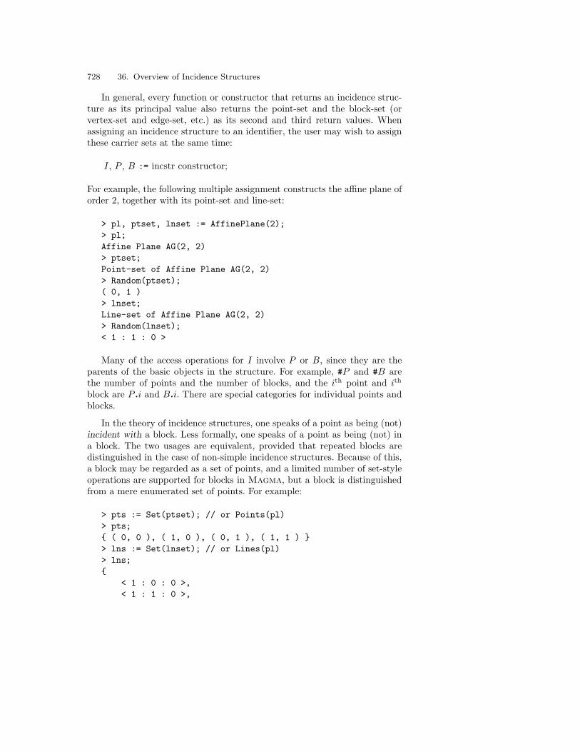
728 36. Overview of Incidence Structures
In general, every function or constructor that returns an incidence struc-ture as its principal value also returns the point-set and the block-set (orvertex-set and edge-set, etc.) as its second and third return values. Whenassigning an incidence structure to an identifier, the user may wish to assignthese carrier sets at the same time:
I, P , B := incstr constructor;
For example, the following multiple assignment constructs the affine plane oforder 2, together with its point-set and line-set:
> pl, ptset, lnset := AffinePlane(2);> pl;Affine Plane AG(2, 2)> ptset;Point-set of Affine Plane AG(2, 2)> Random(ptset);( 0, 1 )> lnset;Line-set of Affine Plane AG(2, 2)> Random(lnset);< 1 : 1 : 0 >
Many of the access operations for I involve P or B, since they are theparents of the basic objects in the structure. For example, #P and #B arethe number of points and the number of blocks, and the ith point and ith
block are P .i and B.i. There are special categories for individual points andblocks.
In the theory of incidence structures, one speaks of a point as being (not)incident with a block. Less formally, one speaks of a point as being (not) ina block. The two usages are equivalent, provided that repeated blocks aredistinguished in the case of non-simple incidence structures. Because of this,a block may be regarded as a set of points, and a limited number of set-styleoperations are supported for blocks in Magma, but a block is distinguishedfrom a mere enumerated set of points. For example:
> pts := Set(ptset); // or Points(pl)> pts; ( 0, 0 ), ( 1, 0 ), ( 0, 1 ), ( 1, 1 ) > lns := Set(lnset); // or Lines(pl)> lns;
< 1 : 0 : 0 >,< 1 : 1 : 0 >,

36.2 Equality and Isomorphism 729
< 1 : 0 : 1 >,< 1 : 1 : 1 >,< 0 : 1 : 0 >,< 0 : 1 : 1 >
> ln := Random(lns); ln;< 0 : 1 : 0 >> Set(ln); ( 0, 0 ), ( 1, 0 )
The function IncidenceMatrix(I) returns the incidence matrix m of I,as an integer matrix with #P rows and #B columns. The matrix entry mij is1 if point i is incident with block j, else 0. For example:
> incmat := IncidenceMatrix(pl);> incmat;[1 1 0 0 1 0][0 0 1 1 1 0][1 0 0 1 0 1][0 1 1 0 0 1]> lnset.4 eq ptset.2, ptset.3;true
36.2 Equality and Isomorphism
Two incidence structures I and J belonging to the same category are equalif the sets of points and blocks over which they are defined are equal. Theexpression I eq J returns true if I equals J , and I ne J returns true if Idoes not equal J .
An isomorphism from an incidence structure I = (PI , BI) to anotherincidence structure J = (PJ , BJ) is a mapping from I to J , such that thepoint-set PI and block-set BI are mapped to PJ and BJ respectively, andthe incidence relation is preserved. The function IsIsomorphic(I, J) returnstrue if I and J are isomorphic. If they are isomorphic, it also returns theisomorphism as a mapping from I to J . For example:
> pl, ptset, lnset := AffinePlane(2);> incmat := IncidenceMatrix(pl);> SwapRows(~incmat, 1, 3);> mypl := AffinePlane< 4 | incmat >;> mypl : Maximal;Affine Plane of order 2

730 36. Overview of Incidence Structures
Points: @ 1, 2, 3, 4 @Lines:
1, 3,3, 4,2, 4,1, 2,2, 3,1, 4
> pl eq mypl;false> y, m := IsIsomorphic(pl, mypl);> y;true> m;Mapping from: PlaneAff: pl to PlaneAff: mypl
The function IsIsomorphic has a parameter AutomorphismGroupswhich can take any of the string values "None", "Left", "Right" (the de-fault), or "Both". It specifies which, if any, of the automorphism groups ofI and J (see below) are to be constructed first. For certain examples, theisomorphism test progresses faster when this parameter is changed from itsdefault value.
36.3 Automorphism Groups and Subgroups
An automorphism of an incidence structure I = (P, B) is an isomorphism ofI onto itself, that is, a mapping such that P and B map to themselves andthe incidence relation is preserved.
36.3.1 Action on Points
The function AutomorphismGroup(I) returns the group of automor-phisms of I, as a permutation group. Magma selects a suitable support forrepresenting the automorphisms as permutations. If there are no repeatedblocks then the support is taken to be P ; otherwise, the support is P ∪ B.However, because of the awkwardness of printing permutations on compli-cated objects, the group that is returned is a permutation group G = Aut(I)on the natural support Ω = 1, 2, . . . , n, where n is the cardinality of thesupport and i ∈ Ω corresponds to the ith element of the support.
The automorphism group G has natural actions on both the point-setand block-set. These actions are provided through use of the G-set mecha-nism. As well as returning the automorphism group G as its principal value,

36.3 Automorphism Groups and Subgroups 731
AutomorphismGroup returns a G-set giving the action of G on the pointsand a G-set giving the action of G on the blocks. Actions of G on the struc-ture may be computed using the G-set versions of orbits, stabilizers, and soon, as described in Chapter 32.
It is often convenient to represent an automorphism of I as a mappingfrom I to I rather than a permutation. For this reason, a fourth and a fifthvalue are returned by AutomorphismGroup: the parent M for all auto-morphisms of I when represented as maps; and a transfer map t from G toM . If g ∈ G is an automorphism represented as a permutation, then thecorresponding map is t(g) or g@t. The parent M and transfer map t canalso be created without calling AutomorphismGroup(I) explicitly by thefunction Aut(I) which returns M and t. In this case, the domain of t is thefull symmetric group of the appropriate degree so an automorphism of I canapplied to by t.
The example below constructs the automorphism group and associatedobjects for the affine plane of order 2. It demonstrates the computation ofimages, orbits and stabilizers, and how to convert the representation of anautomorphism of the plane from an element of G into a mapping:
> pl, ptset, lnset := AffinePlane(2);> G, gspt, gsln, pm, t := AutomorphismGroup(pl);> G;Permutation group G acting on a set of cardinality 4Order = 24 = 2^3 * 3
(2, 4)(2, 3)(1, 2)(3, 4)
> gspt, gsln;GSet ( 0, 0 ), ( 1, 0 ), ( 0, 1 ), ( 1, 1 ) GSet
< 1 : 0 : 0 >,< 1 : 1 : 0 >,< 1 : 0 : 1 >,< 1 : 1 : 1 >,< 0 : 1 : 0 >,< 0 : 1 : 1 >
> pm;Set of all automorphisms of Affine Plane AG(2, 2)> t;Mapping from: GrpPerm: G to PowMap: pm
> g := Random(G); g;(1, 4)(2, 3)

732 36. Overview of Incidence Structures
> Image(g, gspt, ptset.2);( 0, 1 )> Image(g, gsln, lnset.1);< 1 : 0 : 1 >> Orbit(G, gsln, lnset.1) eq gsln;true> Stabilizer(G, gsln, lnset.2);Permutation group acting on a set of cardinality 4
(2, 3)(1, 4)(2, 3)
> au := t(g); au;Mapping from: PlaneAff: pl to PlaneAff: pl> au(lnset.5);< 0 : 1 : 1 >> au(ptset.2) eq ptset.3;true
36.3.2 Action on Blocks
The function BlockGroup(I), EdgeGroup(I), or LineGroup(I) (depend-ing on the nomenclature in the category of I) returns the automorphism groupof I in its action on the blocks of I, as a permutation group acting on a setwhose cardinality is the number of blocks of I. The function also returns theG-set of the blocks. It may be more convenient to use this function ratherthan AutomorphismGroup when the emphasis is on the blocks rather thanthe points. For example, the line group of the plane pl is the automorphismgroup of pl in its action on the 6 lines of pl :
> LG := LineGroup(pl);> LG;Permutation group LG acting on a set of cardinality 6Order = 24 = 2^3 * 3
(2, 5)(4, 6)(1, 5)(3, 6)(1, 3)(2, 4)
36.3.3 Subgroups of the Automorphism Group
Let I be any incidence structure except for a graph or digraph. If I is verylarge, then the computation of the automorphism group G of I may be toodifficult to accomplish in a reasonable time. For such situations, Magma

36.3 Automorphism Groups and Subgroups 733
offers functions that compute certain subgroups of G. These functions areparticularly helpful when the user wishes to know whether the whole groupG is non-trivial.
The function AutomorphismGroupStabilizer(I, k) calculates the sub-group of the automorphism group G that fixes the first k base points, andthe function AutomorphismSubgroup(I) calculates a subgroup of G gen-erated by one element. Each of them returns five values: the subgroup itself;and the four auxiliary values as returned by AutomorphismGroup(I).


37. Graphs
A graph consists of vertices joined by edges. Simple graphs are those in whichno pair of vertices is joined by an edge more than once and no edge is a loopback to the same vertex. In directed graphs (digraphs), each edge has adirection from one vertex to the other; in undirected graphs, the edge has nodirection.
Any simple graph, whether directed or undirected, may be constructed inMagma, but digraphs will not be discussed here. In this chapter, therefore,the term graph will denote an undirected simple graph.
37.1 Constructing Graphs
Magma represents an [undirected simple] graph by stating, for each vertex,the vertices to which it is joined by an edge. For example:
> print PolygonGraph(6);
GraphVertex Neighbours
1 2 6 ;2 1 3 ;3 2 4 ;4 3 5 ;5 4 6 ;6 1 5 ;
The output shows that each vertex in this graph has two neighbours. Forinstance, vertex 3 has neighbours 2 and 4, meaning that there are edgesbetween 3 and 2 and between 3 and 4. Pairs of vertices joined by an edge aresaid to be adjacent.

736 37. Graphs
Table 37.1. Standard graphs
Magma Meaning
CompleteGraph(p) Complete graph Kp on p vertices
BipartiteGraph(m, n) Complete bipartite graph Km,n, i.e., the graph ofm+n vertices such that m of the vertices are joinedto all of the other n vertices, and vice versa
MultipartiteGraph(Q) Complete multipartite graph Km1,...,mr , whereQ = [m1, . . . , mr], i.e., the graph of m1 + · · ·+ mr
vertices such that the vertices in each partite set ofmi vertices are all joined to all the other vertices
EmptyGraph(p) Graph on p vertices and with no edges
KCubeGraph(k) Graph of the k-dimensional cube, Qk
PathGraph(p) Path graph on p vertices, i.e., the graph whose onlyedges are vi, vi+1 where 1 ≤ i < p
PolygonGraph(p) Polygon graph on p vertices, i.e., path graph withextra edge v1, vp
RandomGraph(p, r) A random graph on p vertices, with probability rthat any given pair of vertices is adjacent
RandomTree(p) A random tree (connected acyclic graph) on pvertices
The example above is of the graph corresponding to a hexagon, with its sixvertices and six edges. It was constructed with one of Magma’s functions forstandard graphs, PolygonGraph. These functions are listed in Table 37.1.
There are several ways of constructing graphs in Magma without usingthe standard functions. The constructor for building a general graph with pvertices is
Graph< p | specification of edges >
There are several ways of giving the edge specification on the right side ofthis constructor. The most important methods are to give a list of sets ofpairs of integers, indicating pairs of adjacent vertices, or to give a sequenceof p sets of integers, indicating the neighbours of each vertex in order. Forexample, the graph on 5 vertices with edges between 1 and 2, 1 and 5, 2 and3, and 2 and 5, can be constructed by stating the edges:
> G := Graph< 5 | 1, 2, 1, 5, 2, 3, 2, 5 >;
or by stating the neighbours of the vertices:
> G := Graph< 5 | [ 2, 5, 1, 3, 5, 2, , 1, 2 ] >;
In either case, the following graph results:

37.2 Sets of Vertices and Edges 737
> print G;
GraphVertex Neighbours
1 2 5 ;2 1 3 5 ;3 2 ;4 ;5 1 2 ;
In the neighbour-sequence method, it is permissible to specify an edge be-tween vi and vj by saying that vi is a neighbour of vj without explicitlysaying also that vj is a neighbour of vi:
> print G eq Graph< 5 | [ 2, 5, 3, 5, , , ] >;true
The edge-list and neighbour-sequence methods may be used together in anedge specification, and graphs of the same order p may also be included.Magma will combine all the edge information to find the edge specificationfor the graph being constructed.
37.2 Sets of Vertices and Edges
Each graph G has a corresponding set of vertices and set of edges. In Magmathese sets can be thought of in two senses. The functions VertexSet(G) andEdgeSet(G) return sets V and E in the special categories VertSet andEdgeSet. These special kinds of sets are also the second and third returnvalues of the Graph constructor:
> G, V, E := Graph< 5 | 1, 2, 1, 5, 2, 3, 2, 5 >;> print V, E;The vertex-set of graph GThe edge-set of graph G> print Category(V), Category(E);VertSet EdgeSet
Secondly, the functions Vertices(G) and Edges(G) return enumerated setswhose universes are V and E respectively:
> Vs := Vertices(G); print Vs;
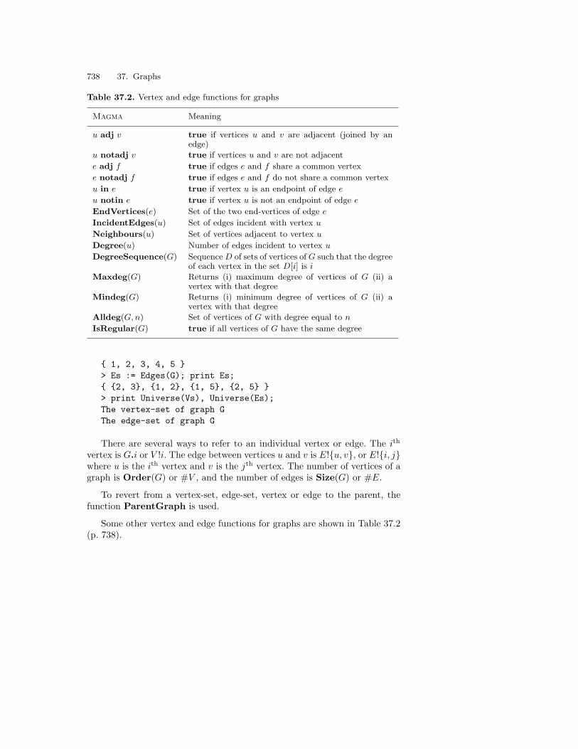
738 37. Graphs
Table 37.2. Vertex and edge functions for graphs
Magma Meaning
u adj v true if vertices u and v are adjacent (joined by anedge)
u notadj v true if vertices u and v are not adjacent
e adj f true if edges e and f share a common vertex
e notadj f true if edges e and f do not share a common vertex
u in e true if vertex u is an endpoint of edge e
u notin e true if vertex u is not an endpoint of edge e
EndVertices(e) Set of the two end-vertices of edge e
IncidentEdges(u) Set of edges incident with vertex u
Neighbours(u) Set of vertices adjacent to vertex u
Degree(u) Number of edges incident to vertex u
DegreeSequence(G) Sequence D of sets of vertices of G such that the degreeof each vertex in the set D[i] is i
Maxdeg(G) Returns (i) maximum degree of vertices of G (ii) avertex with that degree
Mindeg(G) Returns (i) minimum degree of vertices of G (ii) avertex with that degree
Alldeg(G, n) Set of vertices of G with degree equal to n
IsRegular(G) true if all vertices of G have the same degree
1, 2, 3, 4, 5 > Es := Edges(G); print Es; 2, 3, 1, 2, 1, 5, 2, 5 > print Universe(Vs), Universe(Es);The vertex-set of graph GThe edge-set of graph G
There are several ways to refer to an individual vertex or edge. The ith
vertex is G.i or V !i. The edge between vertices u and v is E!u, v, or E!i, jwhere u is the ith vertex and v is the jth vertex. The number of vertices of agraph is Order(G) or #V , and the number of edges is Size(G) or #E.
To revert from a vertex-set, edge-set, vertex or edge to the parent, thefunction ParentGraph is used.
Some other vertex and edge functions for graphs are shown in Table 37.2(p. 738).

37.3 Creating New Graphs 739
37.3 Creating New Graphs
Once a graph G has been constructed, other graphs may be built from it.All of the construction methods described below return three values: the newgraph, its vertex-set and its edge-set.
37.3.1 Addition and Subtraction
One method of creating a new graph from an existing graph G is to addor subtract edges, or to subtract vertices. To add an edge means to makea pair of vertices adjacent, and to subtract an edge means to remove theedge between a pair of vertices. The syntax for these operations is G+ u, vand G − e. To subtract a vertex means to remove a vertex, thus causing arenumbering of the vertices unless the vertex being removed is the highest-numbered one, and of course to remove the edges involving the vertex. Thesyntax for this is G− v. For example:
> print G + G.3, G.4; // add an edge
GraphVertex Neighbours
1 2 5 ;2 1 3 5 ;3 2 4 ;4 3 ;5 1 2 ;
> print G - G.2; // remove a vertex
GraphVertex Neighbours
1 4 ;2 ;3 ;4 1 ;
A set of edges may be added or subtracted in the same way as a singleedge, and a set of vertices may be subtracted in the same way as a singlevertex. Therefore care must be taken not to confuse a set of two vertices withan edge. In particular, G−u, v is G with vertices u and v removed, whereasG− E!u, v is G with the edge u, v removed:

740 37. Graphs
> print G - G.1, G.5; // remove two vertices
GraphVertex Neighbours
1 2 ;2 1 ;3 ;
> print G - E!G.1, G.5; // remove an edge
GraphVertex Neighbours
1 2 ;2 1 3 5 ;3 2 ;4 ;5 2 ;
37.3.2 Subgraph
The sub constructor for graphs has a vertex version and an edge version:
sub< G | list of vertices >sub< G | list of edges >
The vertex version creates the subgraph of graph G containing the listedvertices (renumbered as necessary), preserving whatever edges are betweenvertices in the list. The edge version creates the subgraph containing all thevertices of G but only those edges that are listed. The lists can contain setsof vertices/edges as well as individual vertices/edges.
For instance, the following statements create and print the subgraph ofthe 3-dimensional cube graph generated by vertices 3, 4, 7 and 8:
> K := KCubeGraph(3);> Ksub := sub< K | K.3, K.4, K.7, K.8 >;> print Ksub;
GraphVertex Neighbours
1 2 3 ;

37.3 Creating New Graphs 741
2 1 4 ;3 1 4 ;4 2 3 ;
This graph is the same as the graph of the 2-dimensional cube (i.e., thesquare):
> print Ksub eq KCubeGraph(2);true
Therefore in the original 3-dimensional cube graph, the four vertices must bethe corners of one of the cube’s faces.
An example of sub in the edge version is the creation of the subgraph ofG (defined above) with edges involving vertex 2. Here v in e tests whether avertex v is one of the two endpoints of an edge e:
> print sub< G | edge: edge in E | G.2 in edge >;
GraphVertex Neighbours
1 2 ;2 1 3 5 ;3 2 ;4 ;5 2 ;
The final example for sub illustrates the constructor using a larger graph.Operations on integer sets are used so as to supply the vertices easily:
> M := MultipartiteGraph([10, 5, 20]);> Msub := sub< M |> M.1, ChangeUniverse(13..30, VertexSet(M)) >;> print Msub;
GraphVertex Neighbours
1 2 3 4 5 6 7 8 9 10 11 12 13 14 15 16 17 18 19 ;2 1 5 6 7 8 9 10 11 12 13 14 15 16 17 18 19 ;3 1 5 6 7 8 9 10 11 12 13 14 15 16 17 18 19 ;4 1 5 6 7 8 9 10 11 12 13 14 15 16 17 18 19 ;5 1 2 3 4 ;6 1 2 3 4 ;

742 37. Graphs
...19 1 2 3 4 ;
Every subgraph is returned as a graph in its own right, but coercion maybe used to relate the vertices and edges of the subgraph to those of the maingraph. For instance, in Msub the vertices numbered 2 and 5 correspond tothose called 13 and 16 in M :
> print VertexSet(M) ! Msub.2;13> print EdgeSet(M) ! Msub.2, Msub.5;13, 16
37.3.3 Quotient Graph
A quotient graph Q is constructed by identifying certain vertices of a graphG. The vertices of G are partitioned into a set of disjoint subsets P1, . . . , Pr
of the vertices whose union is the whole vertex-set of G. The vertices of Qcorrespond to the subsets Pi, and two vertices of Q are adjacent if somevertex in the subset corresponding to one is adjacent to some vertex in theother subset. The Magma constructor for the quotient graph is
quo< G | P1, . . . , Pr >
For example, in the cube graph K constructed above, the vertices 3, 4, 7 and8, which are the corners of a face, may be identified:
> Q := quo< K | 3, 4, 7, 8, 1, 2, 5, 6 >;> print Q;
GraphVertex Neighbours
1 2 3 4 ;2 1 3 5 ;3 1 2 4 5 ;4 1 3 5 ;5 2 3 4 ;
From the output, vertex 3 of Q corresponds to the subset of cardinality 4 givenin the partition, vertices 4 and 5 correspond to vertices 5 and 6 in K, andvertices 1 and 2 have the same numbers as their counterparts. The functionContract(S), in Table 37.3 (p. 743), would also construct this graph.

37.3 Creating New Graphs 743
37.3.4 Some Standard Constructions
Table 37.3. Standard related graphs
Magma Meaning
Complement(G) Graph whose edges are exactly those between the non-adjacent vertices of G
Contract(u, v) Given vertices u and v of G, returns the graph which is Gwith u and v identified
Contract(e) Given an edge e = u, v of G, returns Contract(u, v)
Contract(S) Given a set S of vertices of G, returns the graph which isG with all these vertices identified
InsertVertex(e) Given an edge e of G, returns the graph which is G witha new degree-2 vertex inserted in e
InsertVertex(T ) Given an set T of edges of G, returns the graph which isG with a new degree-2 vertex inserted in each edge in T
LineGraph(G) Line graph of the non-empty graph G
Switch(u) Given a vertex u of G, returns the graph which is G butwith the neighbours of u becoming its non-neighbours
Switch(S) Given a set S of vertices of G, returns the graph which isG with Switch(u) applied to it for each vertex u in S
Table 37.3 (p. 743) and Table 37.4 (p. 744) list some other ways of con-structing graphs from existing graphs G and H in Magma.
In the union and product functions given in Table 37.4 (p. 744), G and Hdenote graphs with vertex-sets VG and VH and edge-sets EG and EH . Thesefunctions manipulate the graphs as if their vertices are disjoint, so that, forexample, the Union function when applied to two copies of the same graphyields a graph with twice as many vertices:
> G := Graph< 5 | 1, 2, 1, 5, 2, 3, 2, 5 >;> print Union(G, G);
GraphVertex Neighbours
1 2 5 ;2 1 3 5 ;3 2 ;4 ;5 1 2 ;6 7 10 ;7 6 8 10 ;

744 37. Graphs
Table 37.4. Graph unions and products
Magma Meaning
Union(G, H), G join H Graph with vertex-set VG∪VH and edge-set EG∪EH
EdgeUnion(G, H) Given G and H with the same order n, return thegraph with order n whose edge-set is EG ∪ EH ,by identifying the vertices of G and H havingcorresponding vertex number
CompleteUnion(G, H) Graph that is Union(G, H) together with edgesu, v, for all u ∈ VG and v ∈ VH
CartesianProduct(G, H) Graph with vertex-set VG × VH and such that 2vertices are adjacent when either the first com-ponents are equal and the second are adjacent,or vice versa
LexProduct(G, H) Graph with vertex-set VG × VH and such thatvertices u1, u2 and v1, v2 are adjacent wheneither u1 and v1 are adjacent, or u1 = v1 and u2
and v2 are adjacent
TensorProduct(G, H) Graph with vertex-set VG × VH and such that2 vertices are adjacent when the first compo-nents are adjacent and the second componentsare adjacent
G^n Graph with vertex-set VG, and such that u andv are adjacent when Distance(u, v) ≤ n
8 7 ;9 ;10 6 7 ;
37.4 Testing Properties of a Graph
Table 37.5 (p. 745) lists several of the functions that test properties of graphs.
37.5 Incidence, Adjacency and Distance Matrices
Several matrices are closely associated with each graph G, including those re-turned by the functions IncidenceMatrix(G), AdjacencyMatrix(G) andDistanceMatrix(G).
If G has p vertices and q edges, then the incidence matrix is a p×q matrixM of 1s and 0s. Each column corresponds to an edge, and contains exactly

37.5 Incidence, Adjacency and Distance Matrices 745
Table 37.5. Some tests on graphs
Magma Meaning
IsBipartite(G) true if G is bipartite
IsComplete(G) true if G is complete
IsPath(G) true if G is a path graph
IsPolygon(G) true if G is a polygon graph
IsTree(G) true if G is connected and has no cycles
IsForest(G) true if G has no cycles (i.e., is the disjoint union of trees)
IsEmpty(G) true if G has no edges
two 1s, in the rows whose numbers are the index numbers of the vertices lyingon that edge. Returning to the earlier example:
> G := Graph< 5 | 1, 2, 1, 5, 2, 3, 2, 5 >; print G;
GraphVertex Neighbours
1 2 5 ;2 1 3 5 ;3 2 ;4 ;5 1 2 ;
> print IncidenceMatrix(G);[1 1 0 0][1 0 1 1][0 0 1 0][0 0 0 0][0 1 0 1]
The columns of the incidence matrix show that G has four edges, joiningvertices 1 and 2, 1 and 5, 2 and 3, and 2 and 5.
It is also possible to go in the opposite direction, constructing a graphfrom an incidence matrix M , with the function IncidenceGraph(M).
The adjacency matrix contains 1s and 0s only, like the incidence matrix,but its dimension is p×p. It lists neighbours of vertices, like the printed formof a graph. The 1s in row i give the vertices that are neighbours of vertex i.For example:
> print AdjacencyMatrix(G);

746 37. Graphs
[0 1 0 0 1][1 0 1 0 1][0 1 0 0 0][0 0 0 0 0][1 1 0 0 0]
The distance matrix is also a p × p symmetric matrix of integers. Theentry at row i, column j gives the distance between vertices i and j of G. Forinstance:
> print DistanceMatrix(G);[ 0 1 2 -1 1][ 1 0 1 -1 1][ 2 1 0 -1 2][-1 -1 -1 0 -1][ 1 1 2 -1 0]
37.6 Distance and Connectedness
Table 37.6. Distance, paths, connectedness
Magma Meaning
Distance(u, v) Length of a shortest path between u and v, or −1 if theyare not connected
Geodesic(u, v) Sequence of vertices defining a shortest path between uand v, or the empty sequence if they are not connected
Ball(u, n) Set of vertices at distance ≤ n from u.
Sphere(u, n) Set of vertices at distance n from u.
Diameter(G) Length of a longest path in G, or−1 if G is not connected
DiameterPath(G) Sequence of vertices defining a longest path in G, or theempty sequence if G is not connected
IsConnected(G) true if between any pair of vertices of G there is a path
Component(u) Subgraph corresponding to the connected component ofthe graph containing vertex u
Components(G) Connected components of G as a sequence of subsets ofvertices
Girth(G) Length of a shortest cycle of G
GirthCycle(G) Sequence of vertices defining a shortest cycle of G
IsEulerian(G) true if there is a cycle visiting each vertex of G exactlyonce (i.e., if all vertices have even degree)

37.7 Vertex Subsets and Colourings 747
Table 37.6 (p. 746) explains functions related to the ideas of distance,paths, cycles and connectedness.
37.7 Vertex Subsets and Colourings
Two types of subsets of vertices are particularly important in graph theory.An independent set of a graph is a subset of vertices such that no two ofthe vertices are adjacent. The subgraph generated by an independent set isempty, that is, it has no edges. By contrast, a clique of a graph is a subsetof vertices such that all the vertices are adjacent to one another. Thus thesubgraph generated by a clique is complete.
There are three functions associated with each of these types of sets ofvertices. CliqueNumber(G) and IndependenceNumber(G) return themaximum number of elements that a clique or independent set of graphG can have. LargestClique(G) and LargestIndependent(G) return anexample. For instance, returning to the large tripartite set M defined above,we have:
> M := MultipartiteGraph([10, 5, 20]);> print CliqueNumber(M);3> print LargestClique(M); 10, 15, 35 > print IndependenceNumber(M);20> print LargestIndependent(M); 16, 17, 18, 19, 20, 21, 22, 23, 24, 25, 26, 27, 28, 29,30, 31, 32, 33, 34, 35
The function Clique(G,n) returns a clique of cardinality at least n. If n islarger than the clique number, an empty set is returned. Independent(G,n)works similarly.
Several problems in graph theory can be expressed in terms of colouringthe vertices or edges of a graph, according to some rule. A frequent task isto determine the minimum number of different colours required such that notwo adjacent vertices have the same colour. ChromaticNumber(G) returnsthis minimum number. If instead the task is to colour the edges such that notwo adjacent edges have the same colour, then ChromaticIndex(G) can beused to find the minimum number of colours required. For example, considerthe graph of the cube:
> K := KCubeGraph(3);

748 37. Graphs
> print ChromaticNumber(K), ChromaticIndex(K);2 3
The vertices of the cube can be coloured with as few as 2 colours, by givingone colour to the vertices on a diagonal of the upper face and on the otherdiagonal of the lower face, and the other colour to the remaining vertices. Asfor the edges of the cube, they cannot be coloured with 2 colours since themaximum degree is greater than 2, but can be coloured with 3 colours, onefor each of the 3 classes of parallel sides.
37.8 Automorphism Group of a Graph
The automorphism group of a graph G is the group of permutations onthe vertices of G resulting in an identical graph. (Equality of graphs in thissense is a stronger property than isomorphism.) The function for constructingthe automorphism group of G is AutomorphismGroup(G). (It has severalparameters, which will not be explained here.)
> M := MultipartiteGraph([10, 5, 20]);> A := AutomorphismGroup(M);> print A;Permutation group A acting on a set of cardinality 35Order = 2^29 * 3^13 * 5^7 * 7^3 * 11 * 13 * 17 * 19
(14, 15)(13, 14)(12, 13)(11, 12)(9, 10)(8, 9)(7, 8)(6, 7)(5, 6)(4, 5)(3, 4)(2, 3)(1, 2)(34, 35)(33, 34)
...(16, 17)
> print CompositionFactors(A);G| Cyclic(2)

37.8 Automorphism Group of a Graph 749
*| Alternating(20)*| Cyclic(2)*| Alternating(10)*| Cyclic(2)*| Alternating(5)1
The ^ operator is used for finding the action of an automorphism on avertex:
> print M.9, A.5;9 (9, 10)> print M.9 ^ A.5;10
The action of an automorphism on a set or sequence of vertices or edges canalso be calculated with the ^ operator.
Another automorphism action which may be calculated is the action onthe graph or a subgraph of it. (When an automorphism acts on a subgraph,the computation is done with respect to the main graph.) However, sinceevery element of the automorphism group acts on the graph or subgraph toreturn an isomorphic graph, the results are not of great interest; each of theseisomorphic graphs, converted to a graph in its own right, is the same as theothers:
> Msub := sub< M |> M.1, ChangeUniverse(13..30, VertexSet(M)) >;> print Msub eq Msub ^ A.Random(1, Ngens(A));true> print Msub ^ A;GSetGraphVertex Neighbours
1 2 3 4 5 6 7 8 9 10 11 12 13 14 15 16 17 18 19 ;2 1 5 6 7 8 9 10 11 12 13 14 15 16 17 18 19 ;...
19 1 2 3 4 ;

750 37. Graphs
> print #(M ^ A), M in (M ^ A);1 true
Once the automorphism group A has been constructed, it may be used inany permutation group operations as desired. Additionally, there are severalgraph functions, such as IsPrimitive(G), that apply to properties of theautomorphism group A of graph G but do not require A to be constructedexplicitly. Table 37.7 (p. 750) lists some of them.
Table 37.7. Automorphism group
Magma Meaning
AutomorphismGroup(G) Returns (i) the automorphism group A of G(ii) the canonical graph of G, if parameterCanonical is true or #G < 500
EdgeGroup(G) Automorphism group of G in its action on theedges
x^a, x^S Image of x under action of automorphism a orsubgroup S of A, where x is a vertex, edge, orset or sequence of vertices or edges of G
H^x Image of graph H under action of x, where x isan element or subgroup of A (including A itself)
IsVertexTransitive(G),IsTransitive(G)
true if automorphism group of G is transitive
IsEdgeTransitive(G) true if edge group of G is transitive
IsPrimitive(G) true if automorphism group of G is primitive
IsSymmetric(G) true if automorphism group of G is symmetric
OrbitsPartition(G) Partition of the vertex-set of G correspondingto orbits of automorphism group A of G
Stabilizer(S, x) Stabilizer of x in the subgroup S of A, where xis a vertex, edge, or set or sequence of verticesor edges
IsDistanceTransitive(G) true if for all vertices u, v, w, t in connectedgraph G such that d(u, v) = d(w, t), there existsa ∈ A such that ua = w and va = t
IsDistanceRegular(G) true if G is distance regular
IntersectionArray(G) Intersection array of distance regular graph G
As an example, consider the 4-dimensional cube graph, which containseight 3-dimensional cube graphs. Magma can be used to find their verticeseasily. The method is to find the orbit of a set of vertices which are knownto generate a 3-dimensional cube graph. The orbit will be all those sets ofvertices generating graphs isomorphic to this graph:
> q4 := KCubeGraph(4);

37.8 Automorphism Group of a Graph 751
> s := VertexSet(q4) | 1, 2, 3, 4, 5, 6, 7, 8 ;> print IsIsomorphic(sub< q4 | s >, KCubeGraph(3));true> A4 := AutomorphismGroup(q4);> print s ^ A4;GSet
1, 2, 3, 4, 9, 10, 11, 12 , 1, 2, 3, 4, 5, 6, 7, 8 , 2, 4, 6, 8, 10, 12, 14, 16 , 1, 2, 5, 6, 9, 10, 13, 14 , 1, 3, 5, 7, 9, 11, 13, 15 , 3, 4, 7, 8, 11, 12, 15, 16 , 9, 10, 11, 12, 13, 14, 15, 16 , 5, 6, 7, 8, 13, 14, 15, 16
The output lists the eight sets of vertices for 3-dimensional cube graphs.
37.8.1 Edge Group
The edge group is a variant of the automorphism group that considers theaction on the edges instead of on the vertices. It is returned by the functionEdgeGroup(G). Just as the degree of the automorphism group is the numberof vertices, the degree of the edge group is the number of edges. For example:
> EG := EdgeGroup(q3); print EG;Permutation group EG acting on a set of cardinality 12
(1, 3, 1, 5)(5, 7, 3, 7)(5, 6, 3, 4)(2, 6,2, 4)(4, 8, 6, 8)
(1, 3, 1, 2)(5, 7, 5, 6)(2, 6, 3, 7)(2, 4,3, 4)(6, 8, 7, 8)
(1, 3, 2, 4)(5, 7, 6, 8)(1, 5, 2, 6)(3, 7,4, 8)
The edge group may be considered explicitly as the action of the automor-phism group on the G-set of the edges:
> A3 := AutomorphismGroup(q3);> print ActionImage(A3, GSet(A3, Edges(q3))) eq EG;true
The function IsEdgeTransitive(G) tests whether the edge group of G istransitive.
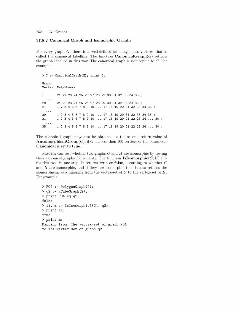
752 37. Graphs
37.8.2 Canonical Graph and Isomorphic Graphs
For every graph G, there is a well-defined labelling of its vertices that iscalled the canonical labelling. The function CanonicalGraph(G) returnsthe graph labelled in this way. The canonical graph is isomorphic to G. Forexample:
> C := CanonicalGraph(M); print C;
GraphVertex Neighbours
1 21 22 23 24 25 26 27 28 29 30 31 32 33 34 35 ;...
20 21 22 23 24 25 26 27 28 29 30 31 32 33 34 35 ;21 1 2 3 4 5 6 7 8 9 10 ... 17 18 19 20 31 32 33 34 35 ;
...30 1 2 3 4 5 6 7 8 9 10 ... 17 18 19 20 31 32 33 34 35 ;31 1 2 3 4 5 6 7 8 9 10 ... 17 18 19 20 21 22 23 24 ... 30 ;
...35 1 2 3 4 5 6 7 8 9 10 ... 17 18 19 20 21 22 23 24 ... 30 ;
The canonical graph may also be obtained as the second return value ofAutomorphismGroup(G), if G has less than 500 vertices or the parameterCanonical is set to true.
Magma can test whether two graphs G and H are isomorphic by testingtheir canonical graphs for equality. The function IsIsomorphic(G, H) ful-fils this task in one step. It returns true or false, according to whether Gand H are isomorphic, and if they are isomorphic then it also returns theisomorphism, as a mapping from the vertex-set of G to the vertex-set of H.For example:
> PG4 := PolygonGraph(4);> q2 := KCubeGraph(2);> print PG4 eq q2;false> ii, m := IsIsomorphic(PG4, q2);> print ii;true> print m;Mapping from: The vertex-set of graph PG4to The vertex-set of graph q2

38. Designs
Magma supports both general incidence structures (category Inc) and threefamilies of incidence structures satisfying stronger conditions, namely near-linear spaces (IncNsp), linear spaces (IncLsp), and t-designs (Dsgn). Thischapter concentrates on the facilities for designs, but explains how to con-struct structures in the other categories as well.
For an introduction to the theory of designs, the reader should consult[AsK92].
38.1 The Categories of Incidence Structures
An incidence structure is a triple (P, B, I) consisting of a set P of points, aset B of blocks, and an incidence relation I which is a subset of P ×B. TheMagma system adopts the usual approach to incidence structures, in whichthe blocks are subsets of P , and I describes which points are in which block.The only difficulty with this approach is the problem of representing repeatedblocks, i.e., two or more blocks consisting of the same set of points; in suchcases Magma considers such blocks to be distinct, although their points arethe same. An incidence structure with no repeated blocks is called simple.An incidence structure is said to be uniform with blocksize k if it has at leastone block and all blocks contain exactly k points. If t ≥ 0, then an incidencestructure is said to be t-balanced if there exists λ ≥ 1 such that each t-subsetof the point set is contained in exactly λ blocks of the structure.
It is usual, when discussing near-linear spaces, to use the term line in placeof the term block. A near-linear space is an incidence structure in which everyline contains at least two points and any two points lie in at most one block.A linear space is a near-linear space in which any two points lie in exactlyone line.
A t-(v, k, λ) design (or t-design) D is a simple incidence structure havingv points, that is uniform with blocksize k and t-balanced for some λ. Notethat a design must contain at least one block. A Steiner design is a t-design

754 38. Designs
with λ = 1. A symmetric design is a t-design where t ≥ 2 and with the samenumber of blocks as points.
38.2 Creating Incidence Structures
Constructors are provided in Magma for the definition of magmas in each ofthe four categories of incidence structures. The category is given by the wordon the left of the constructor: IncidenceStructure, NearLinearSpace,LinearSpace, or Design, designating the categories Inc, IncNsp, IncLspand Dsgn respectively. Within the angle bracket delimiters, the set of pointsis defined on the left side of the | symbol, while the set of blocks is specifiedon the right side of the | symbol:
constructor-name< point-set description | block-set description >
For designs only, the value of t must also be given on the left side, before thepoints are specified:
Design< t, point-set specification | block-set specification >
In all the categories except the general category Inc, the set of blocks issubject to certain restrictions, as explained below. The constructor returnsthree values: the incidence structure (in whichever category was requested);the point-set; and the block-set (also known as the line-set for the categoriesIncNsp and IncLsp).
The ways in which the points and blocks may be described in the con-structor are as follows. The v points may be described in two ways:
– As an indexed set P of cardinality v, giving the set of points directly;
– As the integer v, in which case the point-set is taken to be @1, . . . , v@.
The b blocks of the structure may be given in three ways:
– As a v × b matrix of zeros and ones (as an element of a matrix space overany coefficient ring), which is interpreted as an incidence matrix for thestructure;
– As a set of codewords of a linear code with length v, in which case theblock set is the set of supports of the codewords;
– As a comma-separated list (in the order of the blocks) in which each itemmay be a subset of P , a block of an existing incidence structure, or asequence or indexed set of either of these.

38.2 Creating Incidence Structures 755
For example, the following statement assigns to S the incidence structurewith points 2, 5, 6 and blocks 5, 6, , and 5. The magma S is thenprinted, using the Maximal printing option so that the points and blocksare displayed:
> S := IncidenceStructure< @ 2,5,6 @ | 5,6, , 5 >;> S : Maximal;Incidence Structure on 3 points with 3 blocksPoints: @ 2, 5, 6 @Blocks:
5, 6,,5
Suppose now that the incidence structure S2 has the same points as Sand its blocks are the blocks of S together with 2 and 5, 6 (again). Thenew structure may be constructed with the aid of the functions Points(S)and Blocks(S), which return the points and blocks of S as indexed sets:
> S2 := IncidenceStructure< Points(S) |> Blocks(S), 2, 5,6 >;> S2 : Maximal;Incidence Structure on 3 points with 5 blocksPoints: @ 2, 5, 6 @Blocks:
5, 6,,5,2,5, 6
> IsSimple(S2);false
The output in the final line verifies that S2 has a repeated block.
As a final example of a general incidence structure, the following state-ment constructs the incidence structure S3 with points @1, . . . , 6@ andblocks 1, . . . , 6, 3, 6, and also assigns the point-set and block-set toP and B. Since the point-set is of the form @1, . . . , v@, it is sufficient togive the size of the point-set, rather than the set itself, on the left side of theconstructor:
> S3, P, B := IncidenceStructure< 6 | 1..6, 3, 6 >;> S3 : Maximal;Incidence Structure on 6 points with 3 blocks

756 38. Designs
Points: @ 1, 2, 3, 4, 5, 6 @Blocks:
1, 2, 3, 4, 5, 6,3,6
> P, B;Point-set of Incidence Structure on 6 points with 3 blocksBlock-set of Incidence Structure on 6 points with 3 blocks
For incidence structures in the categories IncNsp and IncLsp, each line(block) must contain at least two points. In a near-linear space, any twopoints must lie in at most one line; in a linear space, any two points mustlie in exactly one line. Magma will test these conditions when the space isconstructed, and will give an error message if they do not hold. For example:
> LS := LinearSpace< 4 | 1,3,4, 1,2, 2,3 >;
>> LS := LinearSpace< 4 | 1,3,4, 1,2, 2,3 >;^
Runtime error in LinearSpace< ... >:Resulting structure is not a linear space> NLS := NearLinearSpace< 4 | 1,3,4, 1,2, 2,3 >;> NLS : Maximal;Near-Linear Space on 4 points with 3 linesPoints: @ 1, 2, 3, 4 @Lines:
1, 3, 4,1, 2,2, 3
> LS := LinearSpace< 4 | 1,3,4, 1,2, 2,3, 2,4 >;> LS : Maximal;Linear Space on 4 points with 4 linesPoints: @ 1, 2, 3, 4 @Lines:
1, 3, 4,1, 2,2, 3,2, 4
The next example demonstrates the construction of a near-linear spacein terms of an incidence matrix; the same principle applies for other inci-dence structures. The columns of the matrix define the lines or blocks of thestructure, as sets of points:
> M := RMatrixSpace(IntegerRing(), 5, 6);

38.2 Creating Incidence Structures 757
> m := M ! [ 0,1,0,0,1,0, 1,1,1,0,0,0, 0,0,1,1,0,1,> 1,0,0,1,1,0, 0,1,0,0,0,1 ];> m;[0 1 0 0 1 0][1 1 1 0 0 0][0 0 1 1 0 1][1 0 0 1 1 0][0 1 0 0 0 1]> Nm := NearLinearSpace< 5 | m >;> Nm : Maximal;Near-Linear Space on 5 points with 6 linesPoints: @ 1, 2, 3, 4, 5 @Lines:
2, 4,1, 2, 5,2, 3,3, 4,1, 4,3, 5
The function IncidenceMatrix(I) returns the incidence matrix of an inci-dence structure I:
> IncidenceMatrix(Nm) eq m;true
For t-designs (incidence structures in the category Dsgn), three condi-tions must hold: no block may be repeated; each block must have the sameblocksize k; and every set of points of cardinality t must lie in the same num-ber λ of blocks. The following example illustrates a way to construct a designusing the function Subsets(T, k), which returns the set of all k-subsets of aset S. In the example, the return value of this function has to be convertedinto a sequence, so that the blocks will be ordered:
> D := Design< 3, 5 | Setseq(Subsets(1..5, 3)) >;> D : Maximal;3-(5, 3, 1) Design with 10 blocksPoints: @ 1, 2, 3, 4, 5 @Blocks:
1, 3, 5,2, 3, 4,1, 4, 5,2, 4, 5,1, 2, 5,1, 2, 3,

758 38. Designs
1, 2, 4,3, 4, 5,2, 3, 5,1, 3, 4
> IncidenceMatrix(D);[1 0 1 0 1 1 1 0 0 1][0 1 0 1 1 1 1 0 1 0][1 1 0 0 0 1 0 1 1 1][0 1 1 1 0 0 1 1 0 1][1 0 1 1 1 0 0 1 1 0]> IsComplete(D);true
The design above is a 3-(5, 3, 1) design, indicating that t is 3, the numberof points v is 5, the blocksize k is 3, and λ is 1. In fact, it is the complete(5, 3, 1) design.
As a second example, let H be the Hamming code over GF(3) with r = 3.The incidence structure formed from the supports of the words of H withweight 5 is a 2-design:
> H := HammingCode(GF(3), 3);> H : Minimal;[13, 10, 3] Hamming code (r = 3) over GF(3)> W5 := Words(H, 5);> DD := Design< 2, 13 | W5 >;> DD;2-(13, 5, 90) Design with 702 blocks
When an incidence structure in a category other than Inc is being built,it is often the case that the user knows from earlier work or from theory thatthe blocks satisfy the conditions for the category. Magma’s default action isto check that the conditions are fulfilled, but this can take a great deal oftime if the structure is large. For this reason, a parameter Check is providedfor the constructors NearLinearSpace, LinearSpace, and Design, so thatthe user can turn off the checking when it would be superfluous. If Checkis assigned false instead of the default value of true, then Magma does notcheck that the conditions required by the category are correct; it is then theuser’s responsibility to ensure that they are. For example, if CG2x is theextended binary Golay code, then the supports of the words of weight 12in CG2x form a 5-design. The time statements below demonstrate that theconstruction of the design is much faster with checking turned off:
> CG2x := GolayCode(GF(2), true);> wds := Words(CG2x, 12);

38.3 Points and Blocks 759
> #wds;2576> time DG := Design<5, Length(CG2x) | wds : Check := false>;Time: 1.410> time DG := Design<5, Length(CG2x) | wds>;Time: 219.781> DG;5-(24, 12, 48) Design with 2576 blocks
38.3 Points and Blocks
Table 38.1. Point-set and block-set functions
Magma Meaning
PointSet(I) Point-set P of incidence structure I
BlockSet(I) Block-set B of incidence structure I
Points(I) Indexed set of points of I
Blocks(I) Indexed set of blocks of I
NumberOfPoints(I), #P Number of points of I
NumberOfBlocks(I), #B Number of blocks of I
Support(I) Indexed set of underlying points of I, intheir original category
Rep(P ) Representative point of point-set P
Random(P ) Random point of point-set P
Rep(B) Representative block of block-set B
Random(B) Random block of block-set B
Point(I, i), P .i ith point of incidence structure I withpoint-set P
Block(I, i), B.i ith block of incidence structure I withblock-set B
P!x Point corresponding to element x of in-dexed set used to create I with point-setP
PointDegrees(I) Sequence whose ith term is the number ofblocks containing point P .i
BlockDegrees(I), BlockSizes(I) Sequence whose ith term is the number ofpoints in block B.i
Covalence(I, S) Given subset S of point-set of I, returnnumber of blocks of I containing S
IncidenceMatrix(I) Incidence matrix of I

760 38. Designs
Table 38.2. Functions for individual blocks
Magma Meaning
Set(b) Set of points in block b
Support(b) Set of underlying points in block b, intheir original category
Rep(b) Representative point in block b
Random(b) Random point in block b
p in b, p notin b true if point p is [not] in block b
S subset b, S notsubset b true if set S of points is [not] in blockb
PointDegree(I, p) Number of blocks of I containing pointp
BlockDegree(I, b), BlockSize(I, b), #b Number of points contained in block bin the incidence structure I
ConnectionNumber(I, p, b) Number of blocks joining p to b in I
IsBlock(I, S) true if set or block S represents a blockof I; if true, also returns one such block
Block(I, p, q), Line(I, p, q) A block of I containing points p and q,if it exists (in a linear space, if p 6= qthen the line exists uniquely)
IsParallelClass(I, b, c) true if there is a parallel class of I con-taining blocks b and c; if true, also re-turns one such class
Let P and B denote the point-set and block-set of an incidence struc-ture I (in any category). As was mentioned above, P and B are given asthe second and third return values of all constructors and functions thatreturn incidence structures. They may also be accessed directly using thefunctions PointSet(I) and BlockSet(I). P and B belong to the specialcategories IncPtSet and IncBlkSet. They are not true Magma sets, butspecial structures which act as the parents for points and blocks respectively.For example, let DG be the design calculated above from the extended binaryGolay code:
> P := PointSet(DG);> B := BlockSet(DG);> P, B;Point-set of 5-(24, 12, 48) Design with 2576 blocksBlock-set of 5-(24, 12, 48) Design with 2576 blocks> Category(P), Category(B);IncPtSet IncBlkSet
There is another pair of functions, Points(I) and Blocks(I), returningthe points and blocks of I explicitly as indexed sets. (The indexing reflects

38.3 Points and Blocks 761
the ordering of the points and the blocks.) The user should take care not toconfuse these functions with PointSet(I) and BlockSet(I). The universesof these sets are P and B, and their elements are in the categories IncPtand IncBlk. For example:
> pts := Points(DG);> pts;@ 1, 2, 3, 4, 5, 6, 7, 8, 9, 10, 11, 12, 13, 14,15, 16, 17, 18, 19, 20, 21, 22, 23, 24 @> blks := Blocks(DG);> #blks;2576> Universe(pts) eq P and Universe(blks) eq B;true> Category(Random(pts)), Category(Random(blks));IncPt IncBlk
One consequence of the fact that special categories are used for points andblocks is that repeated blocks can be handled correctly by the system. If theblocks of a non-simple incidence structure are printed, the result seems to bean indexed set containing more than one copy of the same element. However,the blocks are internally distinct; it is only their printed forms that are thesame. For example:
> Irpt := IncidenceStructure< 4 | 1,3, 3,4, 3,4 >;> BL := Blocks(Irpt); BL;@ 1, 3, 3, 4, 3, 4 @> BL[2] eq BL[3];false
Although the category of each block is IncBlk, not SetEnum, blocks maybe treated as normal sets for most purposes. For example, the operators in,join, meet and subset are available. However, in some circumstances a blockhas to be converted into a true enumerated set of points, using the functionSet:
> BL2set := Set(BL[2]);> Category(BL2set);SetEnum> BL2set; 3, 4 > Universe(BL2set) eq PointSet(Irpt);true

762 38. Designs
A third way of regarding points and blocks is in terms of the universe ofthe set of points used in the creation of I (often the integer ring). The functionSupport(I) may be applied to the whole structure I to return the indexedset of the points in the original universe. Similarly, Support(b), given anindividual block b, returns the set of the points in the block, in the originaluniverse. For example:
> supp := Support(DG);> supp;@ 1, 2, 3, 4, 5, 6, 7, 8, 9, 10, 11, 12, 13, 14,15, 16, 17, 18, 19, 20, 21, 22, 23, 24 @> Universe(supp);Integer Ring
> bl5 := B.5;> bl5;5, 6, 7, 8, 11, 13, 16, 18, 19, 20, 22, 23> Support(bl5); 5, 6, 7, 8, 11, 13, 16, 18, 19, 20, 22, 23 > Universe($1);Integer Ring
It should be noted that if the set of points is other than @1, . . . , v@ thenthere is a distinction between the ith point and the point called i (if indeedsuch a point exists). For example, in the structure below, the point called 2is the first point, and the second point is the point called 5:
> S, P, B := IncidenceStructure< @ 2,5,6 @ |> 5,6, , 5 >;> pt := P!2; pt;2> Index(Points(S), pt);1> P.2;5
Table 38.1 lists operators and functions connected with the points andblocks of an incidence structure I, and Table 38.2 lists operations whichapply to an individual block b. They include functions for random and rep-resentative elements of the point-set, the block-set, and a block, and for thenumber of points in a block and the number of blocks containing a point.Most of these are straightforward to apply, once the user understands thedistinction between the point-set and the indexed set of points (and similarlyfor blocks), and the way that Magma uses special categories for points andblocks.

38.4 Elementary Invariants of a Design 763
38.4 Elementary Invariants of a Design
Table 38.3. Elementary invariants of a design
Magma Meaning
Parameters(D) Parameters of t-(v, b, r, k, λ) design D, asa record with fieldnames t, v, b, r, k,lambda
ReplicationNumber(D) Replication number r (t > 0)
BlockDegree(D), BlockSize(D) Number k of points in each block of D
Covalence(D, s) Number λs of blocks containing an arbi-trary s-subset of the points of D
IntersectionNumber(D, i, j) Block intersection number λji (i + j ≤ t)
Order(D) Order λ11 of D (t ≥ 2)
PascalTriangle(D) ‘Pascal triangle’ of D
The conditions satisfied by the blocks of a design D imply the existenceof certain invariants for D. The functions in Table 38.3 return these values.
The fundamental parameters for a design D are: t; v, the number of points;b, the number of blocks; r, the replication number, which is defined as thenumber of blocks containing any point of D, where t > 0; k, the blocksize;and λ. Some of these parameters may be obtained individually from particu-lar functions, but they are also available collectively from Parameters(D).It returns a record whose fieldnames are the names of the parameters. Forexample:
> DD := Design< 2, 13 | Words(HammingCode(GF(3), 3), 5) >;> DD;2-(13, 5, 90) Design with 702 blocks> pp := Parameters(DD);> pp;rec<recformat<t, v, b, r, k, lambda> | t := 2, v := 13,b := 702, r := 270, k := 5, lambda := 90>> pp‘r;270> pp‘lambda;90
Some of the functions in the table involve the block intersection numberλj
i . This quantity is defined for integers i and j such that i + j ≤ t, and itequals the number of blocks of D that contain an i-set but are disjoint froma j-set. For example, PascalTriangle(D) returns a ‘Pascal triangle’ whose

764 38. Designs
rows are of the form λi−10 , λi−2
1 , . . . , λ0i−1. The triangle has k + 1 rows if D
is a Steiner design, or t + 1 rows otherwise. The return value of the functionis a sequence whose terms are the rows, also stored as sequences. However,when this triangle is printed, it is displayed in a formatted style:
> CG2x := GolayCode(GF(2), true);> DG := Design<5, Length(CG2x) | Words(CG2x, 12) :> Check := false >;> pt := PascalTriangle(DG);> pt[4];[ 280, 336, 336, 280 ]> pt;
25761288 1288
616 672 616280 336 336 280
120 160 176 160 12048 72 88 88 72 48
38.5 Incidence Structures with Particular Properties
Table 38.4 summarizes the functions that test whether a given incidencestructure, of any category, has a certain property. The table also lists booleanfunctions that may be applied to designs or (near-)linear spaces only.
Two of the functions, IsBalanced(I, t) and IsDesign(I, t), have a pa-rameter Al so that the user can specify which algorithm should be followedwhen testing if I is balanced with respect to t. The default value of Alis "NoOrbits", meaning a ‘brute force’ test. The alternative algorithm is"Orbits", which uses the orbits of t-sets under the automorphism group ofI; this is much faster for some cases, but slower for others. For example:
> CG2x := GolayCode(GF(2), true);> incDG8 := IncidenceStructure< Length(CG2x) |> Words(CG2x, 8) >;> time IsBalanced(incDG8, 4);true 5Time: 16.241> // redefine incDG8 for a new test> incDG8 := IncidenceStructure< Length(CG2x) |> Words(CG2x, 8) >;> time IsBalanced(incDG8, 4 : Al := "Orbits");true 5
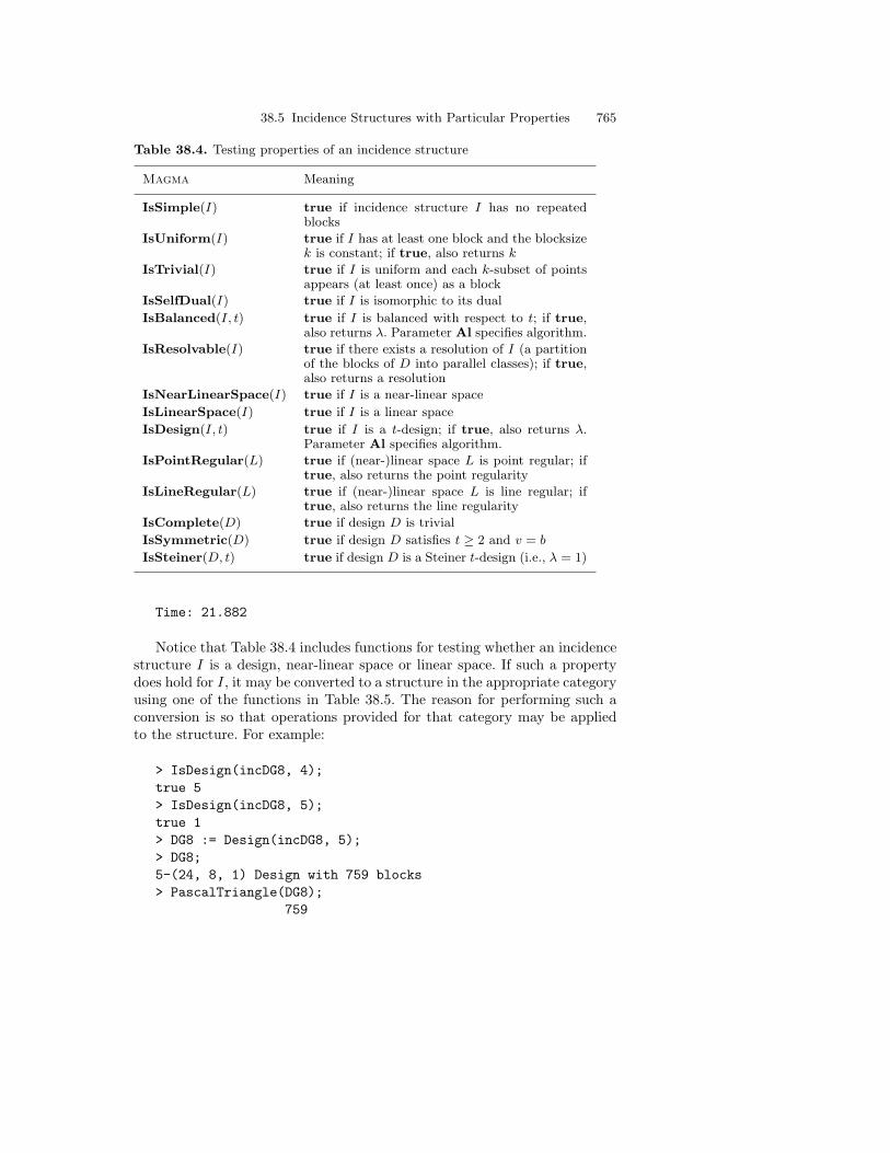
38.5 Incidence Structures with Particular Properties 765
Table 38.4. Testing properties of an incidence structure
Magma Meaning
IsSimple(I) true if incidence structure I has no repeatedblocks
IsUniform(I) true if I has at least one block and the blocksizek is constant; if true, also returns k
IsTrivial(I) true if I is uniform and each k-subset of pointsappears (at least once) as a block
IsSelfDual(I) true if I is isomorphic to its dual
IsBalanced(I, t) true if I is balanced with respect to t; if true,also returns λ. Parameter Al specifies algorithm.
IsResolvable(I) true if there exists a resolution of I (a partitionof the blocks of D into parallel classes); if true,also returns a resolution
IsNearLinearSpace(I) true if I is a near-linear space
IsLinearSpace(I) true if I is a linear space
IsDesign(I, t) true if I is a t-design; if true, also returns λ.Parameter Al specifies algorithm.
IsPointRegular(L) true if (near-)linear space L is point regular; iftrue, also returns the point regularity
IsLineRegular(L) true if (near-)linear space L is line regular; iftrue, also returns the line regularity
IsComplete(D) true if design D is trivial
IsSymmetric(D) true if design D satisfies t ≥ 2 and v = b
IsSteiner(D, t) true if design D is a Steiner t-design (i.e., λ = 1)
Time: 21.882
Notice that Table 38.4 includes functions for testing whether an incidencestructure I is a design, near-linear space or linear space. If such a propertydoes hold for I, it may be converted to a structure in the appropriate categoryusing one of the functions in Table 38.5. The reason for performing such aconversion is so that operations provided for that category may be appliedto the structure. For example:
> IsDesign(incDG8, 4);true 5> IsDesign(incDG8, 5);true 1> DG8 := Design(incDG8, 5);> DG8;5-(24, 8, 1) Design with 759 blocks> PascalTriangle(DG8);
759
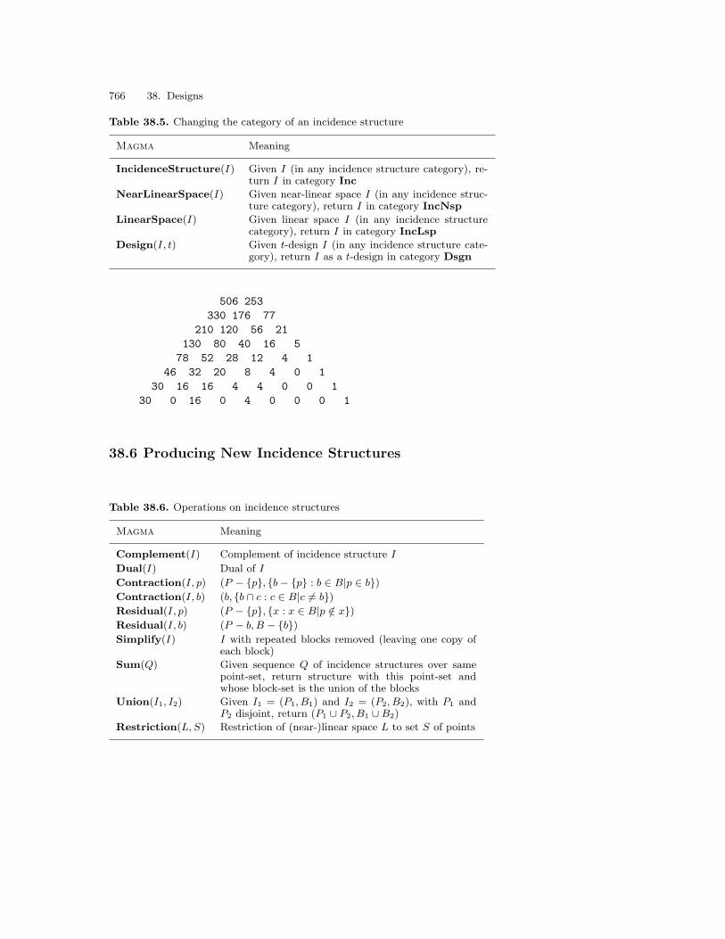
766 38. Designs
Table 38.5. Changing the category of an incidence structure
Magma Meaning
IncidenceStructure(I) Given I (in any incidence structure category), re-turn I in category Inc
NearLinearSpace(I) Given near-linear space I (in any incidence struc-ture category), return I in category IncNsp
LinearSpace(I) Given linear space I (in any incidence structurecategory), return I in category IncLsp
Design(I, t) Given t-design I (in any incidence structure cate-gory), return I as a t-design in category Dsgn
506 253330 176 77
210 120 56 21130 80 40 16 5
78 52 28 12 4 146 32 20 8 4 0 1
30 16 16 4 4 0 0 130 0 16 0 4 0 0 0 1
38.6 Producing New Incidence Structures
Table 38.6. Operations on incidence structures
Magma Meaning
Complement(I) Complement of incidence structure I
Dual(I) Dual of I
Contraction(I, p) (P − p, b− p : b ∈ B|p ∈ b)Contraction(I, b) (b, b ∩ c : c ∈ B|c 6= b)Residual(I, p) (P − p, x : x ∈ B|p /∈ x)Residual(I, b) (P − b, B − b)Simplify(I) I with repeated blocks removed (leaving one copy of
each block)
Sum(Q) Given sequence Q of incidence structures over samepoint-set, return structure with this point-set andwhose block-set is the union of the blocks
Union(I1, I2) Given I1 = (P1, B1) and I2 = (P2, B2), with P1 andP2 disjoint, return (P1 ∪ P2, B1 ∪B2)
Restriction(L, S) Restriction of (near-)linear space L to set S of points

38.7 Standard Constructions for Designs 767
Table 38.6 lists functions that may be used to produce new incidencestructures from a given incidence structure I with point-set P and block-setB, where p or b denote a point or block of I. The notation (π, β) denotes theresulting incidence structure, with point-set π and block-set β.
For example, the Fano plane may be considered as a 2-(7, 3, 1) design.Since it is symmetric, its dual is a design with the same parameters. However,the Dual function does not return a design with the optimal t, since to doso in general might be very expensive computationally; that value must befound ‘by hand’:
> fano := Design< 2, 7 | 1,2,3, 1,4,5, 1,6,7,> 2,4,7, 2,5,6, 3,5,7, 3,4,6 >;> fano;2-(7, 3, 1) Design with 7 blocks> IsSymmetric(fano);true> du := Dual(fano);> du;0-(7, 3, 7) Design with 7 blocks> du2 := Design(du, 2);> du2;2-(7, 3, 1) Design with 7 blocks
38.7 Standard Constructions for Designs
Table 38.7. Witt and Hadamard designs
Magma Meaning
WittDesign(12) 5-(12, 6, 1) Witt design (small Mathieudesign)
WittDesign(24) 5-(24, 8, 1) Witt design (large Mathieudesign)
IsHadamard(M) true if matrix ring element M (over anyring) is a Hadamard matrix
IsHadamardEquivalent(H, J) true if Hadamard matrices H and J areHadamard equivalent
HadamardRowDesign(H, i) Hadamard 3-design corresponding to rowi of H, where H is an n × n Hadamardmatrix with n ≥ 4
HadamardColumnDesign(H, i) Hadamard 3-design corresponding to ith
column i of H, where H is as above

768 38. Designs
Two of the most famous examples of designs are the Witt (or Mathieu)designs and the Hadamard designs. Magma’s functions for constructing theseare listed in Table 38.7. WittDesign(n) accepts two values for its argument,n = 12 and n = 24:
> W12 := WittDesign(12); W12;5-(12, 6, 1) Design with 132 blocks> W24 := WittDesign(24); W24;5-(24, 8, 1) Design with 759 blocks
The Hadamard functions relate to the construction of a 3-design from aHadamard matrix, which is a square matrix with orthogonal rows and con-taining only ±1 as its entries. Thus an m×m matrix M is a Hadamard matrixif all entries are ±1 and MM t = mIm, where Im is the m×m identitiy matrix.For example:
> H := MatrixRing(IntegerRing(), 8) !> [ 1, 1, 1, 1, 1, 1, 1, 1,> 1, 1, 1, 1, -1, -1, -1, -1,> 1, 1, -1, -1, 1, 1, -1, -1,> 1, 1, -1, -1, -1, -1, 1, 1,> 1, -1, 1, -1, 1, -1, -1, 1,> 1, -1, 1, -1, -1, 1, 1, -1,> 1, -1, -1, 1, -1, 1, -1, 1,> 1, -1, -1, 1, 1, -1, 1, -1] ;> IsHadamard(H);true> HRD := HadamardRowDesign(H, 5);> HRD : Maximal;3-(8, 4, 1) Design with 14 blocksPoints: @ 1, 2, 3, 4, 5, 6, 7, 8 @Blocks:
1, 3, 5, 8,1, 3, 6, 7,1, 4, 5, 7,1, 4, 6, 8,1, 2, 3, 4,1, 2, 7, 8,1, 2, 5, 6,2, 4, 6, 7,2, 4, 5, 8,2, 3, 6, 8,2, 3, 5, 7,5, 6, 7, 8,3, 4, 5, 6,

38.8 Difference Sets and Their Development 769
3, 4, 7, 8> HRD eq HadamardColumnDesign(H, 2);true
38.8 Difference Sets and Their Development
Table 38.8. Difference sets and their developments
Magma Meaning
DifferenceSet(p, t) Difference set of type given by string t and cor-responding to prime p, where t is "Q", "H6", "T","B", "B0", "O", "O0", or "W4" and the choice of timposes conditions on p
SingerDifferenceSet(n, q) Singer difference set corresponding to a hyper-plane of PG(n, q)
IsDifferenceSet(B) true if B is a difference set over ZZ/mZZ or aniterable finite group; if true, also returns λ, thenumber of times each non-identity group/ring el-ement appears as a ‘difference’ of elements of B
Development(B) Given set B which is a difference set relative toA, where A is ZZ/mZZ or a finite group, returnthe symmetric design with point set A and whoseblocks consist of the sets obtained by translatingB by each element of A in turn
Development(T ) Given difference family T = B1, . . . , Bl wherethe Bi are difference sets relative to A [as above],return the incidence structure with point set Aand whose ith block is the set B1 ∪ · · · ∪ Bltranslated by the ith element of A
Let G be a group of order v. A (v, k, λ)-difference set for G is a k-subset Dof G such that the multiset * gh−1 : g, h ∈ D | g 6= h * contains every non-identity element of G exactly λ times. Difference sets may be used to generateincidence structures by means of the process known as development.
The Magma functions for difference sets and their developments areshown in Table 38.8. In the case of the function DifferenceSet(p, t), thepossible values for the string t have the interpretations as given by MarshallHall in [Hal86], pp. 141–142. A difference set produced by this function orby the function SingerDifferenceSet will have a residue class ring as itsuniverse, in which case the set has the additive form g−h : g, h ∈ D|g 6= h.For the functions that operate on an existing (or putative) difference set,the group G may be represented either additively by a residue class ring

770 38. Designs
or abelian group, or multiplicatively by a finite group in any other groupcategory in which iteration is possible (i.e., other than GrpFP).
In the following example, the difference set D constructed is of type "H6"with p = 43. The multiset operations are used to verify that D is a differenceset with λ = 10, and then a design is constructed from D:
> D := DifferenceSet(43, "H6");> D; 1, 2, 3, 32, 4, 33, 5, 35, 37, 8, 39, 11, 41,12, 42, 16, 19, 20, 21, 22, 27 > Universe(D);Residue class ring of integers modulo 43> _, lambda := IsDifferenceSet(D);> lambda;10
> // check> diffs := * g - h : g, h in D | g ne h *;> diffs;* 29^^10, 1^^10, 30^^10, 2^^10, 31^^10, 3^^10, 32^^10,33^^10, 4^^10, 5^^10, 34^^10, 6^^10, 35^^10, 36^^10,7^^10, 8^^10, 37^^10, 9^^10, 38^^10, 39^^10, 10^^10,40^^10, 11^^10, 41^^10, 12^^10, 42^^10, 13^^10, 14^^10,15^^10, 16^^10, 17^^10, 18^^10, 19^^10, 20^^10, 21^^10,22^^10, 23^^10, 24^^10, 25^^10, 26^^10, 27^^10, 28^^10 *> #Set(diffs) eq (43 - 1);true
> dv := Development(D);> dv;2-(43, 21, 10) Design with 43 blocks
Difference sets may also be constructed using group theory; the followingexample is adapted from [LiW92], pp. 198, 345, 348. Suppose that D is anynormalized (21, 5, 1)-difference set in ZZ/21ZZ, if such a difference set exists. Itfollows from the Multiplier Theorem for difference sets that D must satisfy2D = D, that is, D equals the set consisting of the elements of D multipliedby 2. Therefore D must be a union of orbits of the mapping x 7→ 2x inZZ/21ZZ, and so all possible difference sets D may be constructed simply bycollecting together orbits of appropriate sizes. In Magma, the orbits may becalculated as the orbits of a permutation group generated by the permutation-representation of this mapping:
> z21 := Set(ResidueClassRing(21));

38.8 Difference Sets and Their Development 771
> G := PermutationGroup< z21 | [2*a : a in z21] >;> orbs := Orbits(G);> orbs;[
GSet 0 ,GSet 13, 5, 17, 19, 20, 10 ,GSet 11, 1, 2, 4, 16, 8 ,GSet 15, 18, 9 ,GSet 12, 3, 6 ,GSet 14, 7
]
From the sizes of the orbits, the only possible difference sets could be D1,the union of the fourth and sixth orbits, or D2, the union of the fifth andsixth orbits. It turns out that D1 is a difference set, and since D2 consistsof the negatives of D1, all the difference sets with the given parameters areequivalent:
> D1 := orbs[4] join orbs[6];> D1; 14, 15, 18, 7, 9 > IsDifferenceSet(D1);true 1> D2 := orbs[5] join orbs[6];> D2 eq -x : x in D1 ;true
The blocks of the development of D1 form a projective plane of order 4:
> dv := Development(D1);> dv;2-(21, 5, 1) Design with 21 blocks> proj := ProjectivePlane(dv);> proj : Maximal;Projective plane of order 4Points: @ 0, 1, 2, 3, 4, 5, 6, 7, 8, 9, 10, 11, 12, 13,14, 15, 16, 17, 18, 19, 20 @Lines:
7, 9, 14, 15, 18,8, 10, 15, 16, 19,9, 11, 16, 17, 20,0, 10, 12, 17, 18,1, 11, 13, 18, 19,2, 12, 14, 19, 20,0, 3, 13, 15, 20,
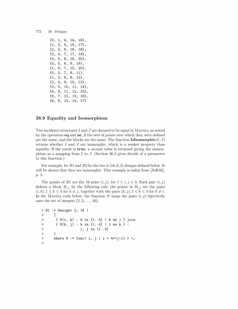
772 38. Designs
0, 1, 4, 14, 16,1, 2, 5, 15, 17,2, 3, 6, 16, 18,3, 4, 7, 17, 19,4, 5, 8, 18, 20,0, 5, 6, 9, 19,1, 6, 7, 10, 20,0, 2, 7, 8, 11,1, 3, 8, 9, 12,2, 4, 9, 10, 13,3, 5, 10, 11, 14,4, 6, 11, 12, 15,5, 7, 12, 13, 16,6, 8, 13, 14, 17
38.9 Equality and Isomorphism
Two incidence structures I and J are deemed to be equal in Magma, as testedby the operators eq and ne, if the sets of points over which they were definedare the same, and the blocks are the same. The function IsIsomorphic(I, J)returns whether I and J are isomorphic, which is a weaker property thanequality. If the result is true, a second value is returned giving the isomor-phism as a mapping from I to J . (Section 36.2 gives details of a parameterto this function.)
For example, let B1 and B2 be the two 2-(16, 6, 2) designs defined below. Itwill be shown that they are isomorphic. This example is taken from [AsK92],p. 5.
The points of B1 are the 16 pairs (i, j), for 1 ≤ i, j ≤ 4. Each pair (i, j)defines a block Bi,j by the following rule: the points in Bi,j are the pairs(i, k), 1 ≤ k ≤ 4 for k 6= j, together with the pairs (k, j), 1 ≤ k ≤ 4 for k 6= i.In the Magma code below, the function N maps the pairs (i, j) bijectivelyonto the set of integers 1, 2, . . . , 16.
> B1 := Design< 2, 16 |> [> N(i, k) : k in [1..4] | k ne j join> N(k, j) : k in [1..4] | i ne k :> i, j in [1..4]> ]> where N := func< i, j | i + 4*(j-1) > >;>

38.9 Equality and Isomorphism 773
> B1 : Maximal;2-(16, 6, 2) Design with 16 blocksPoints: @ 1, 2, 3, 4, 5, 6, 7, 8, 9, 10, 11,12, 13, 14, 15, 16 @Blocks:
2, 3, 4, 5, 9, 13,1, 6, 7, 8, 9, 13,1, 5, 10, 11, 12, 13,1, 5, 9, 14, 15, 16,1, 3, 4, 6, 10, 14,2, 5, 7, 8, 10, 14,2, 6, 9, 11, 12, 14,2, 6, 10, 13, 15, 16,1, 2, 4, 7, 11, 15,3, 5, 6, 8, 11, 15,3, 7, 9, 10, 12, 15,3, 7, 11, 13, 14, 16,1, 2, 3, 8, 12, 16,4, 5, 6, 7, 12, 16,4, 8, 9, 10, 11, 16,4, 8, 12, 13, 14, 15
The design B2 is constructed from the complete graph K6 on six vertices.The points are the 15 edges of K6, together with another point denoted by∞.The first ten blocks comprise the edges of those subgraphs of K6 that consistof two disjoint triangles. The remaining six blocks are formed by taking eachvertex v of K6 in turn, and forming the set comprising the edges incidentwith v and ∞. In the code below the points are renumbered 1 to 16.
> inf := 16;> S := 1..6 ;> E := SetToIndexedSet(Subsets(S, 2));> I := func< x | Index(E, x) >;> triangles := func< T |> I(U) : U in Subsets(T, 2) join> I(U) : U in Subsets(S diff T, 2) >;> claw := func< i |> Include( I(i, j) : j in [1..6] | i ne j , inf) >;> B2 := Design< 2, 16 |> [ triangles(1,j,k) : k in [j+1..6], j in [2..5] ]> cat [ claw(i) : i in [1..6] ] >;> B2 : Maximal;2-(16, 6, 2) Design with 16 blocksPoints: @ 1, 2, 3, 4, 5, 6, 7, 8, 9, 10, 11,12, 13, 14, 15, 16 @

774 38. Designs
Blocks:1, 6, 7, 9, 10, 12,7, 8, 10, 11, 14, 15,2, 3, 6, 10, 13, 15,4, 5, 9, 10, 13, 14,1, 3, 4, 7, 8, 13,1, 2, 4, 6, 11, 14,1, 3, 5, 9, 11, 15,2, 4, 8, 9, 12, 15,3, 5, 6, 8, 12, 14,2, 5, 7, 11, 12, 13,1, 2, 5, 8, 10, 16,3, 4, 10, 11, 12, 16,1, 12, 13, 14, 15, 16,6, 8, 9, 11, 13, 16,2, 3, 7, 9, 14, 16,4, 5, 6, 7, 15, 16
Now B1 and B2 may be tested for isomorphism, using IsIsomorphic. Thesecond return value of this function is an isomorphism from B1 to B2.
> flag, m := IsIsomorphic(B1, B2);> flag;true> m;Mapping from: Dsgn: B1 to Dsgn: B2> [<i, m(i)>: i in Points(B1)];[ <1, 1>, <2, 6>, <3, 7>, <4, 16>, <5, 12>, <6, 3>, <7, 15>,<8, 9>, <9, 2>, <10, 5>, <11, 8>, <12, 11>, <13, 13>,<14, 14>, <15, 10>, <16, 4> ]
38.10 Automorphism Group
Table 38.9 lists the major operations associated with the automorphism groupof an incidence structure I. Section 36.3 explains these and other operationsin more detail, including the multiple values returned by the group functions.
For example:
> D := WittDesign(24);> IsPointTransitive(D) and IsBlockTransitive(D);true> A, gspt, gsbl := AutomorphismGroup(D);

38.10 Automorphism Group 775
Table 38.9. Automorphism group functions
Magma Meaning
AutomorphismGroup(I) If incidence structure I is simple, returns auto-morphism group of I in its action on the point-set; otherwise, returns automorphism group of Iin its action on the union of the point-set and theblock-set
PointGroup(I) Automorphism group of I in its action on thepoint-set
BlockGroup(I) Automorphism group of I in its action on theblock-set
IsPointTransitive(I) true if automorphism group of I acts transitivelyon point-set of I
IsBlockTransitive(I) true if automorphism group of I acts transitivelyon block-set of I
> FactoredOrder(A);[ <2, 10>, <3, 3>, <5, 1>, <7, 1>, <11, 1>, <23, 1> ]> a := Random(A); a;(2, 7, 17, 24, 13, 20, 23, 5, 18, 16, 21, 11, 12, 4, 6,
14, 10, 22, 8, 9, 19, 15, 3)> p5 := Point(D, 5); p5;5> Image(a, gspt, p5);18> b6 := Block(D, 6); b6;8, 11, 17, 18, 19, 20, 22, 24> Image(a, gsbl, b6);8, 9, 12, 13, 15, 16, 23, 24> A3 := SylowSubgroup(A, 3);> Orbit(A3, gspt, p5);GSet 12, 23, 5, 6, 18, 20, 21, 22, 11
Notice that if I is not simple, then AutomorphismGroup(I) acts onboth the points and the blocks, so the degree of the group is the sum of thenumber of points and the number of blocks. For example:
> S2 := IncidenceStructure< @ 2,5,6 @ |> 5,6, , 5, 2, 5,6 >;> G := AutomorphismGroup(S2);> G;Permutation group G acting on a set of cardinality 8Order = 2
(4, 8)

776 38. Designs
38.11 Relationship to Graphs and Linear Codes
Table 38.10. Incidence structures, graphs and codes
Magma Meaning
IncidenceStructure(G) Incidence structure I corresponding to graph G,where blocks of D correspond to edges of G
PointGraph(I) Point graph G of incidence structure I, where ver-tices of G are points of I, and vertices u, v ∈ G areadjacent if both u and v are in a block of I
BlockGraph(I) Point graph of dual of I
IncidenceGraph(I) Incidence graph (bipartite) of incidence structureI, with vertex set the union of the point set andblock set of I, and with point p being adjacent toblock b whenever p ∈ b
LinearCode(I, K) Given incidence structure I with v points, and fi-nite field K, return linear code of length v gen-erated by characteristic functions of blocks of Iconsidered as vectors of K(v)
Incidence structures, graphs and linear codes possess close combinato-rial relationships. Table 38.10 lists the functions for transferring between agraph and an incidence structure, and the function for converting an inci-dence structure into a code. In addition, recall from Section 38.2 that a setof words from a linear code may be used to generate an incidence structure.
For example, the code over GF(2) generated by the Fano plane is isomor-phic to the Hamming code with r = 3:
> fano := Design< 2, 7 | 1,2,3, 1,4,5, 1,6,7,> 2,4,7, 2,5,6, 3,5,7, 3,4,6 >;> C := LinearCode(fano, GF(2));> C;[7, 4, 3] Linear Code over GF(2)Generator matrix:[1 0 0 0 0 1 1][0 1 0 0 1 1 0][0 0 1 0 1 0 1][0 0 0 1 1 1 1]> IsIsomorphic(C, HammingCode(GF(2), 3));true (2, 7, 3, 6)
39. Finite Planes
In its facilities for finite geometry, Magma supports both projective planes(category PlaneProj) and affine planes (PlaneAff). Within these cate-gories, there are special operations for classical planes, that is, planes de-fined over a 2-dimensional vector space (for affine planes) or a 3-dimensionalvector space (for projective planes). Note that Magma’s operations for cre-ating and manipulating planes bear strong resemblance to those for incidencestructures.
For an introduction to the theory, the reader should consult [HuP73].
39.1 Constructing Projective and Affine Planes
In Magma, there are three main ways to construct a projective or affineplane: from an incidence relation involving points and lines that obeys theappropriate axioms; from a pre-existing incidence structure (in any category)that obeys the appropriate axioms; or from a vector space over a finite field.Some Magma operations on planes are only possible if the plane has beenconstructed explicitly from a vector space; such planes will be called classicalhere.
All these methods of construction return the plane as the principal returnvalue, in the category PlaneProj or PlaneAff as requested. They also pro-vide the point-set and the line-set of the plane as the second and third returnvalues. The point-set and line-set belong to special categories PlanePtSetand PlaneLnSet. Although called the point-set and line-set, they are nottrue Magma sets, but structures which act as the parent structures for pointsand lines respectively.
39.1.1 Planes from Incidence Relations
A finite plane may be described by v points and b lines, where the linesare sets of points. For a projective plane, the incidence relation between the
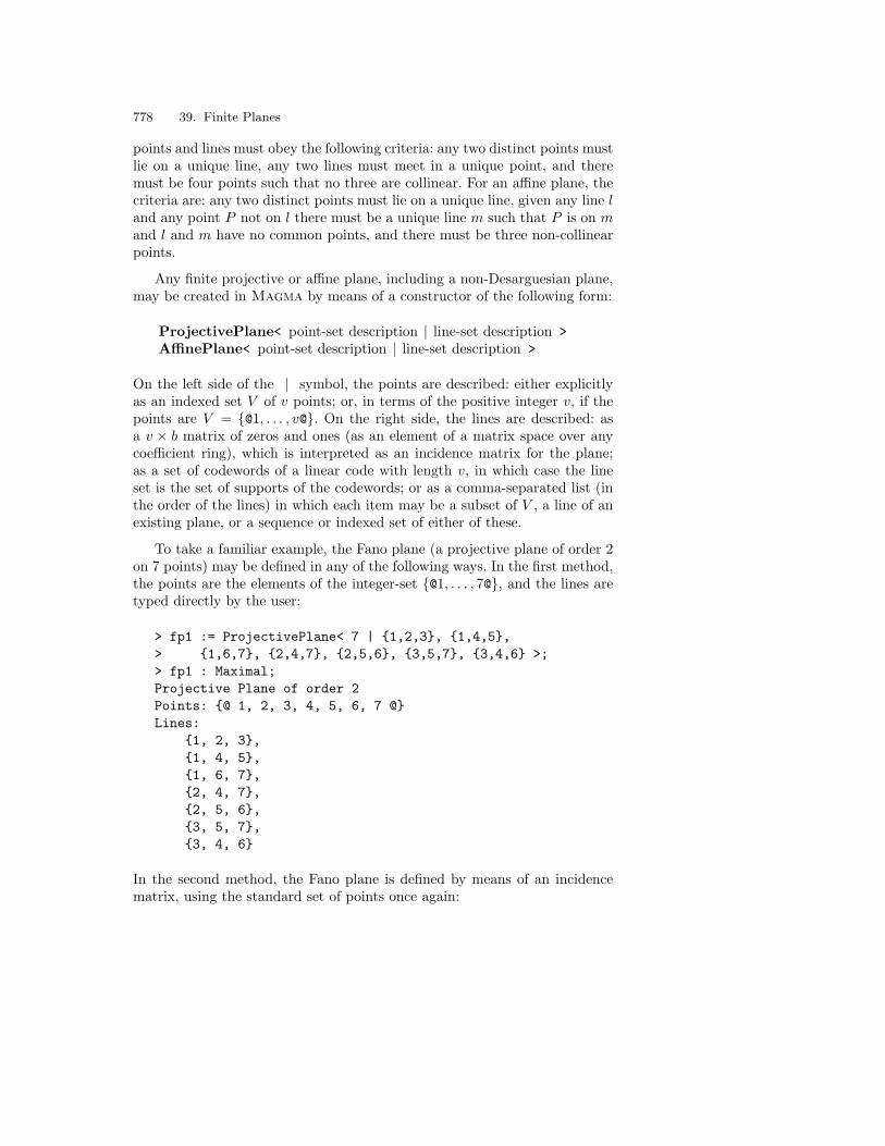
778 39. Finite Planes
points and lines must obey the following criteria: any two distinct points mustlie on a unique line, any two lines must meet in a unique point, and theremust be four points such that no three are collinear. For an affine plane, thecriteria are: any two distinct points must lie on a unique line, given any line land any point P not on l there must be a unique line m such that P is on mand l and m have no common points, and there must be three non-collinearpoints.
Any finite projective or affine plane, including a non-Desarguesian plane,may be created in Magma by means of a constructor of the following form:
ProjectivePlane< point-set description | line-set description >AffinePlane< point-set description | line-set description >
On the left side of the | symbol, the points are described: either explicitlyas an indexed set V of v points; or, in terms of the positive integer v, if thepoints are V = @1, . . . , v@. On the right side, the lines are described: asa v × b matrix of zeros and ones (as an element of a matrix space over anycoefficient ring), which is interpreted as an incidence matrix for the plane;as a set of codewords of a linear code with length v, in which case the lineset is the set of supports of the codewords; or as a comma-separated list (inthe order of the lines) in which each item may be a subset of V , a line of anexisting plane, or a sequence or indexed set of either of these.
To take a familiar example, the Fano plane (a projective plane of order 2on 7 points) may be defined in any of the following ways. In the first method,the points are the elements of the integer-set @1, . . . , 7@, and the lines aretyped directly by the user:
> fp1 := ProjectivePlane< 7 | 1,2,3, 1,4,5,> 1,6,7, 2,4,7, 2,5,6, 3,5,7, 3,4,6 >;> fp1 : Maximal;Projective Plane of order 2Points: @ 1, 2, 3, 4, 5, 6, 7 @Lines:
1, 2, 3,1, 4, 5,1, 6, 7,2, 4, 7,2, 5, 6,3, 5, 7,3, 4, 6
In the second method, the Fano plane is defined by means of an incidencematrix, using the standard set of points once again:

39.1 Constructing Projective and Affine Planes 779
> incmat := RMatrixSpace(IntegerRing(), 7, 7) !> [1,1,1,0,0,0,0, 1,0,0,1,1,0,0, 1,0,0,0,0,1,1,> 0,1,0,1,0,0,1, 0,1,0,0,1,1,0, 0,0,1,0,1,0,1,> 0,0,1,1,0,1,0 ];> incmat;[1 1 1 0 0 0 0][1 0 0 1 1 0 0][1 0 0 0 0 1 1][0 1 0 1 0 0 1][0 1 0 0 1 1 0][0 0 1 0 1 0 1][0 0 1 1 0 1 0]> fp2 := ProjectivePlane< 7 | incmat >;
In the third and final method, the points are the elements of ZZ/7ZZ (labelled 0to 6), and the lines are all triples of the form a, a+1, a+3, where a ∈ ZZ/7ZZ:
> Z7 := ResidueClassRing(7);> pts := SetToIndexedSet(Set(Z7));> lns := @ a, a+1, a+3 : a in pts @;> fp3 := ProjectivePlane< pts | lns >;> fp3 : Maximal;Projective Plane of order 2Points: @ 0, 1, 2, 3, 4, 5, 6 @Lines:
0, 1, 3,1, 2, 4,2, 3, 5,3, 4, 6,0, 4, 5,1, 5, 6,0, 2, 6
As an example of an affine plane, let C be the full vector space of dimen-sion 4 over GF(2), regarded as a linear code, and consider the order-2 affineplane constructed from the codewords of weight 2. The lines of the resultingstructure are the same as the 2-subsets of @1, . . . , 4@:
> C := LinearCode(VectorSpace(GF(2), 4));> A1 := AffinePlane< 4 | Words(C, 2) >;> A1 : Maximal;Affine Plane of order 2Points: @ 1, 2, 3, 4 @Lines:
1, 3,

780 39. Finite Planes
1, 4,2, 4,2, 3,3, 4,1, 2
> A2 := AffinePlane< 4 | Setseq(Subsets(1..4, 2)) >;> A2 : Maximal;Affine Plane of order 2Points: @ 1, 2, 3, 4 @Lines:
1, 3,1, 4,2, 4,2, 3,1, 2,3, 4
> A1 eq A2;true
When a plane is being built using one of these constructors, the user oftenknows from earlier work or from theory that the lines satisfy the conditionsfor the category. Magma provides a parameter Check for the constructorsProjectivePlane and AffinePlane so that the user can stop the systemchecking that the conditions are satisfied. If Check is assigned false, insteadof its default value true, then Magma will not check the conditions, so theuser must ensure that they are true. This technique will save a consider-able amount of time if the plane is large, and is especially recommended forstructures which are loaded into Magma from previously generated files.
39.1.2 Planes from Incidence Structures
Suppose that I is an incidence structure, in any of the incidence struc-ture categories. If I has the properties of an affine plane, then it may beconverted to an affine plane in the PlaneAff category using the functionAffinePlane(I). Similarly, if I has the properties of a projective plane, thenit may be converted to the category PlaneProj by means of the functionProjectivePlane(I).
For example, a projective plane of order 5 whose points are the elementsof ZZ/31ZZ may be constructed from the development [a kind of design] of aSinger difference set with n = 2 and q = 5:
> sds := SingerDifferenceSet(2, 5); sds;

39.1 Constructing Projective and Affine Planes 781
0, 1, 3, 14, 26, 10 > sdv := Development(sds); sdv;2-(31, 6, 1) Design with 31 blocks> spp := ProjectivePlane(sdv);> Universe(Support(spp));Residue class ring of integers modulo 31> spp : Maximal;Projective Plane of order 5Points: @ 0, 1, 2, 3, 4, 5, 6, 7, 8, 9, 10,11, 12, 13, 14, 15, 16, 17, 18, 19, 20,21, 22, 23, 24, 25, 26, 27, 28, 29, 30 @Lines:
0, 1, 3, 10, 14, 26,1, 2, 4, 11, 15, 27,2, 3, 5, 12, 16, 28,3, 4, 6, 13, 17, 29,4, 5, 7, 14, 18, 30,0, 5, 6, 8, 15, 19,1, 6, 7, 9, 16, 20,2, 7, 8, 10, 17, 21,3, 8, 9, 11, 18, 22,4, 9, 10, 12, 19, 23,5, 10, 11, 13, 20, 24,6, 11, 12, 14, 21, 25,7, 12, 13, 15, 22, 26,8, 13, 14, 16, 23, 27,9, 14, 15, 17, 24, 28,10, 15, 16, 18, 25, 29,11, 16, 17, 19, 26, 30,0, 12, 17, 18, 20, 27,1, 13, 18, 19, 21, 28,2, 14, 19, 20, 22, 29,3, 15, 20, 21, 23, 30,0, 4, 16, 21, 22, 24,1, 5, 17, 22, 23, 25,2, 6, 18, 23, 24, 26,3, 7, 19, 24, 25, 27,4, 8, 20, 25, 26, 28,5, 9, 21, 26, 27, 29,6, 10, 22, 27, 28, 30,0, 7, 11, 23, 28, 29,1, 8, 12, 24, 29, 30,0, 2, 9, 13, 25, 30

782 39. Finite Planes
39.1.3 Classical Planes from Vector Spaces
Every Desarguesian projective or affine plane bears a strong relationship tosome vector space over a finite field. Magma provides special functions fordefining such planes, as explained below, and any plane defined in this waywill be described here as a classical plane. A few Magma operations on planesare only available for classical planes, and will not work for a plane definedotherwise, even if it happens to be Desarguesian.
Let W be a 3-dimensional vector space defined over the field F = GF(q),where q is a prime power. Then there exists a classical projective planeP of order n = q defined by the one-dimensional and two-dimensionalsubspaces of W . P may be created in Magma by any of the functionsProjectivePlane(W ), ProjectivePlane(F ), or ProjectivePlane(q). Thepoints and lines of classical projective planes are printed by Magma in a spe-cial way: the points are given by 3 colon-separated field elements, surroundedby parentheses; the lines are also given by 3 colon-separated field elements,but are surrounded by angle brackets. A line 〈a : b : c〉 may be interpreted asthe line given by the equation ax + by + cz = 0. For example, the followinglines construct the classical projective plane of order 27, then demonstratethe appearance of points and lines:
> F<w> := GF(27); F;Finite field of size 3^3> P27, VP27, LP27 := ProjectivePlane(F);> P27;Projective Plane PG(2, 27)> VP27, LP27;Point-set of Projective Plane PG(2, 27)Line-set of Projective Plane PG(2, 27)
> pt := Random(VP27);> pt;( 1 : w^7 : w^10 )> ln := Random(LP27);> ln;< 1 : w^6 : w^19 >> Set(ln); ( 1 : w^4 : 1 ), ( 1 : w^9 : w^19 ), ( 1 : w^18 : 2 ),( 1 : w^8 : w^10 ), ( 0 : 1 : 1 ), ( 1 : w^12 : w ), ( 1 :w^11 : w^14 ), ( 1 : w^16 : w^8 ), ( 1 : w^7 : 0 ), ( 1 :w^15 : w^6 ), ( 1 : 1 : w^5 ), ( 1 : w^17 : w^18 ), ( 1 :w^21 : w^3 ), ( 1 : 2 : w^17 ), ( 1 : w^23 : w^21 ), ( 1 :w^20 : w^7 ), ( 1 : w^6 : w^22 ), ( 1 : w^24 : w^12 ), ( 1: w^3 : w^23 ), ( 1 : w^22 : w^15 ), ( 1 : w^5 : w^4 ), (
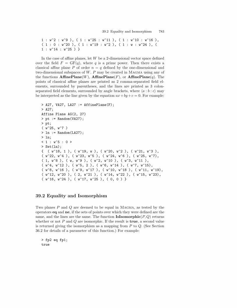
39.2 Equality and Isomorphism 783
1 : w^2 : w^9 ), ( 1 : w^25 : w^11 ), ( 1 : w^10 : w^16 ),( 1 : 0 : w^20 ), ( 1 : w^19 : w^2 ), ( 1 : w : w^24 ), (1 : w^14 : w^25 )
In the case of affine planes, let W be a 2-dimensional vector space definedover the field F = GF(q), where q is a prime power. Then there exists aclassical affine plane P of order n = q defined by the one-dimensional andtwo-dimensional subspaces of W . P may be created in Magma using any ofthe functions AffinePlane(W ), AffinePlane(F ), or AffinePlane(q). Thepoints of classical affine planes are printed as 2 comma-separated field el-ements, surrounded by parentheses, and the lines are printed as 3 colon-separated field elements, surrounded by angle brackets, where 〈a : b : c〉 maybe interpreted as the line given by the equation ax+by+c = 0. For example:
> A27, VA27, LA27 := AffinePlane(F);> A27;Affine Plane AG(2, 27)> pt := Random(VA27);> pt;( w^25, w^7 )> ln := Random(LA27);> ln;< 1 : w^5 : 0 >> Set(ln); ( w^18, 1 ), ( w^19, w ), ( w^20, w^2 ), ( w^21, w^3 ),( w^22, w^4 ), ( w^23, w^5 ), ( w^24, w^6 ), ( w^25, w^7),( 1, w^8 ), ( w, w^9 ), ( w^2, w^10 ), ( w^3, w^11 ),( w^4, w^12 ), ( w^5, 2 ), ( w^6, w^14 ), ( w^7, w^15),( w^8, w^16 ), ( w^9, w^17 ), ( w^10, w^18 ), ( w^11, w^19),( w^12, w^20 ), ( 2, w^21 ), ( w^14, w^22 ), ( w^15, w^23),( w^16, w^24 ), ( w^17, w^25 ), ( 0, 0 )
39.2 Equality and Isomorphism
Two planes P and Q are deemed to be equal in Magma, as tested by theoperators eq and ne, if the sets of points over which they were defined are thesame, and the lines are the same. The function IsIsomorphic(P,Q) returnswhether or not P and Q are isomorphic. If the result is true, a second valueis returned giving the isomorphism as a mapping from P to Q. (See Section36.2 for details of a parameter of this function.) For example:
> fp2 eq fp1;true

784 39. Finite Planes
> fp1 eq fp3;false> ii, m:= IsIsomorphic(fp1, fp3);> ii;true> m;Mapping from: PlaneProj: fp1 to PlaneProj: fp3
39.3 Points and Lines
39.3.1 General Point and Line Operations
Table 39.1. Point-set and line-set functions
Magma Meaning
IncidenceMatrix(P ) Incidence matrix of P
PointSet(P ) Point-set V of plane P
LineSet(P ) Line-set L of plane P
Points(P ) Indexed set of points of P
Lines(P ) Indexed set of lines of P
NumberOfPoints(P ), #V Number of points of P
NumberOfLines(P ), #L Number of lines of P
Support(P ) Indexed set of underlying points of P , in theiroriginal category
Rep(V ) Representative point of point-set V
Random(V ) Random point of point-set V
Rep(L) Representative line of line-set L
Random(L) Random line of line-set L
ParentPlane(x) Plane for which x is the point-set, the line-set, apoint or a line
V .i ith point of plane P with point-set V
L.i ith line of plane P with line-set L
V !x Point corresponding to element x of support ofP , where V is point-set of P (if P is classical, xmust be a vector)
L!S Given line-set L of plane P and set or sequenceS of collinear points, return line containing S
Table 39.1 (p. 784) lists the functions associated with the point-set Vand line-set L of a projective or affine plane P . As was mentioned above,V and L are given as the second and third return values of all constructors
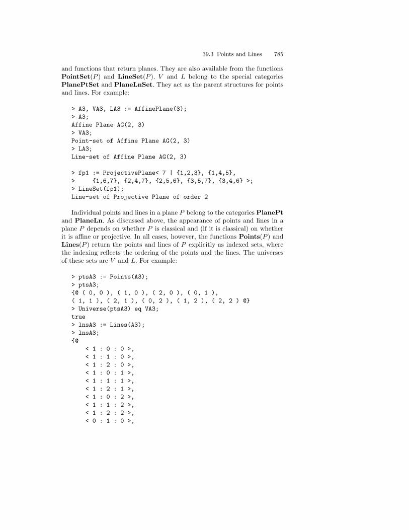
39.3 Points and Lines 785
and functions that return planes. They are also available from the functionsPointSet(P ) and LineSet(P ). V and L belong to the special categoriesPlanePtSet and PlaneLnSet. They act as the parent structures for pointsand lines. For example:
> A3, VA3, LA3 := AffinePlane(3);> A3;Affine Plane AG(2, 3)> VA3;Point-set of Affine Plane AG(2, 3)> LA3;Line-set of Affine Plane AG(2, 3)
> fp1 := ProjectivePlane< 7 | 1,2,3, 1,4,5,> 1,6,7, 2,4,7, 2,5,6, 3,5,7, 3,4,6 >;> LineSet(fp1);Line-set of Projective Plane of order 2
Individual points and lines in a plane P belong to the categories PlanePtand PlaneLn. As discussed above, the appearance of points and lines in aplane P depends on whether P is classical and (if it is classical) on whetherit is affine or projective. In all cases, however, the functions Points(P ) andLines(P ) return the points and lines of P explicitly as indexed sets, wherethe indexing reflects the ordering of the points and the lines. The universesof these sets are V and L. For example:
> ptsA3 := Points(A3);> ptsA3;@ ( 0, 0 ), ( 1, 0 ), ( 2, 0 ), ( 0, 1 ),( 1, 1 ), ( 2, 1 ), ( 0, 2 ), ( 1, 2 ), ( 2, 2 ) @> Universe(ptsA3) eq VA3;true> lnsA3 := Lines(A3);> lnsA3;@
< 1 : 0 : 0 >,< 1 : 1 : 0 >,< 1 : 2 : 0 >,< 1 : 0 : 1 >,< 1 : 1 : 1 >,< 1 : 2 : 1 >,< 1 : 0 : 2 >,< 1 : 1 : 2 >,< 1 : 2 : 2 >,< 0 : 1 : 0 >,
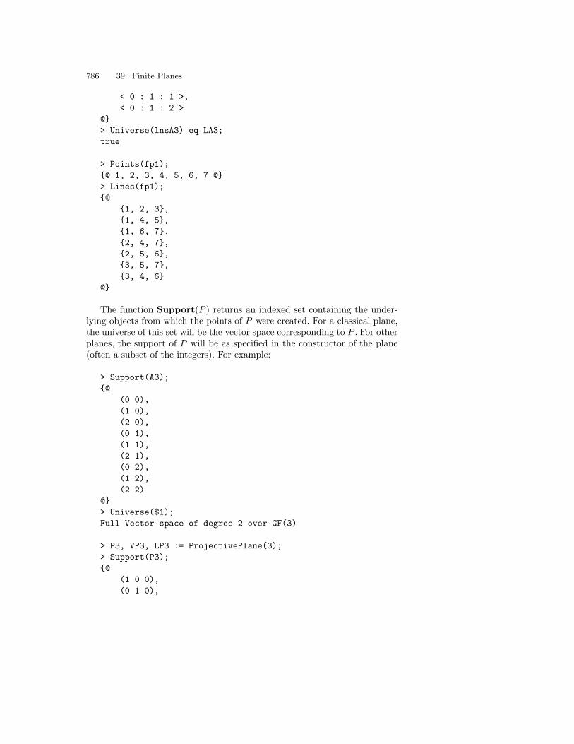
786 39. Finite Planes
< 0 : 1 : 1 >,< 0 : 1 : 2 >
@> Universe(lnsA3) eq LA3;true
> Points(fp1);@ 1, 2, 3, 4, 5, 6, 7 @> Lines(fp1);@
1, 2, 3,1, 4, 5,1, 6, 7,2, 4, 7,2, 5, 6,3, 5, 7,3, 4, 6
@
The function Support(P ) returns an indexed set containing the under-lying objects from which the points of P were created. For a classical plane,the universe of this set will be the vector space corresponding to P . For otherplanes, the support of P will be as specified in the constructor of the plane(often a subset of the integers). For example:
> Support(A3);@
(0 0),(1 0),(2 0),(0 1),(1 1),(2 1),(0 2),(1 2),(2 2)
@> Universe($1);Full Vector space of degree 2 over GF(3)
> P3, VP3, LP3 := ProjectivePlane(3);> Support(P3);@
(1 0 0),(0 1 0),

39.3 Points and Lines 787
(0 0 1),(1 2 0),(0 1 2),(1 2 1),(1 1 1),(1 1 2),(1 0 1),(1 1 0),(0 1 1),(1 2 2),(1 0 2)
@> Universe($1);Full Vector space of degree 3 over GF(3)
> Support(fp1);@ 1, 2, 3, 4, 5, 6, 7 @> Universe($1);Integer Ring
The ith point and the ith line of P are returned respectively by V .i andL.i, where V is the point-set of P and L is the line-set. (The same resultsmay be obtained by indexing the return values of Points(P ) and Lines(P ).)A further way to construct a point is to coerce an element x of the supportinto V , using the expression V !x. For example:
> VA3.6;( 2, 1 )> LA3.7;< 1 : 0 : 2 >
> PointSet(fp1) ! 6;6> Category($1);PlanePt
The following example illustrates some of the point and line functions,by converting the classically-defined affine plane AG2(3) into a general affineplane:
> A3 := AffinePlane(3);> A3;Affine Plane AG(2, 3)> pts := Points(A3);> lns := [ Index(pts, p) : p in Set(ll) :

788 39. Finite Planes
> ll in Lines(A3) ];> myA3 := AffinePlane< #pts | lns >;> myA3 : Maximal;Affine Plane of order 3Points: @ 1, 2, 3, 4, 5, 6, 7, 8, 9 @Lines:
1, 4, 7,1, 6, 8,1, 5, 9,3, 6, 9,3, 5, 7,3, 4, 8,2, 5, 8,2, 4, 9,2, 6, 7,1, 2, 3,7, 8, 9,4, 5, 6
> A3 eq myA3;false> IsIsomorphic(A3, myA3);trueMapping from: PlaneAff: A3 to PlaneAff: myA3
The functions relating to concepts of collinearity, concurrency, and paral-lelism are given in Table 39.2 (p. 789).
Note the distinction between Set(l) and Support(l), where l is a line ofP . Set(l) returns the points of l as points, whereas Support(l) returns themin their original category. For example:
> l := Rep(LA3); l;< 1 : 0 : 0 >> Set(l), Support(l); ( 0, 0 ), ( 0, 1 ), ( 0, 2 )
(0 0),(0 2),(0 1)
> l := Rep(LP3); l;< 1 : 0 : 0 >> Set(l), Support(l); ( 0 : 1 : 0 ), ( 0 : 0 : 1 ),

39.3 Points and Lines 789
Table 39.2. Concurrency, collinearity, and parallel classes
Magma Meaning
Rep(l) Representative point from line l
Random(l) Random point from line l
p in l, p notin l true if point p is [not] on line l
S subset l, S notsubset l true if set S of points is [not] on line l
l meet m Unique point common to lines l and m
IsCollinear(P, S) true if points of P in set S are collinear; iftrue, also returns the line which they define
IsConcurrent(P, S) true if lines of P in set S are concurrent; iftrue, also returns the common point
Pencil(P, p) Set of all lines through point p in plane P
Set(l) Set of all points on line l
Support(l) Set of underlying points on line l, in their orig-inal category
ContainsQuadrangle(P, S) true if set S of points of P contains aquadrangle
IsParallel(P, l, m) true if lines l and m of affine plane P areparallel
ParallelClass(P, l) Set of all lines parallel to line l of affine planeP
ParallelClasses(P ) Set of classes of parallel lines partitioning affineplane P
( 0 : 1 : 2 ), (0 : 1 : 1 )
(0 1 1),(0 1 2),(0 1 0),(0 0 1)
> l := Rep(LineSet(fp1)); l;1, 2, 3
> Set(l), Universe(Set(l)); 1, 2, 3 Point-set of Projective Plane of order 2
> Support(l), Universe(Support(l)); 1, 2, 3 Integer Ring

790 39. Finite Planes
39.3.2 Operations for Classical Planes
Table 39.3. Functions for classical planes over finite fields
Magma Meaning
VectorSpace(P ) Vector space underlying classical plane P
Field(P ) (Finite) field K over which P is defined
V !x Point corresponding to element x of vector space used tocreate P , where V is point-set of P
V ![a, b, c] Given point-set V of P = PG2(K), and sequence [a, b, c]of elements of K, return point (a : b : c) in P
V ![a, b] Given point-set V of P = AG2(K), and sequence [a, b] ofelements of K, return point (a, b) in P
Eltseq(p) Coordinates of point p as sequence of elements of K([a, b, c] for PG2(K); [a, b] for AG2(K))
Coordinates(P, p) Coordinates of point p in plane P as sequence of elementsof K ([a, b, c] for PG2(K); [a, b] for AG2(K))
p[i] ith component of point p, where p is represented as (a : b :c) in PG2(K) or (a, b) in AG2(K)
L![a, b, c] Given line-set L of classical plane P defined over K, andsequence [a, b, c] of elements of K, return line 〈a : b : c〉in P (i.e., line given by equation ax + by + cz = 0 forPG2(K), or ax + by + c = 0 for AG2(K))
Eltseq(l) Coordinates of line l as sequence [a, b, c] of elements of K
Coordinates(P, l) Coordinates of line l in plane P as sequence [a, b, c] ofelements of K
l[i] ith component of line l, where l is represented as 〈a : b : c〉L![m, b] Given line-set L of P = AG2(K), and sequence [m, b] of
elements of K, return line in P given by equation y =mx + b
Slope(l) Slope of line l in AG2(K)
Table 39.3 (p. 790) lists additional functions for classical planes. Most ofthem relate to the coordinates of a point or line, and their relationship to thevector space from which the plane P is constructed.
In order to use these operations correctly in the projective case, it isessential to note that if P = PG2(q), then there are (q − 1) non-zero vectorscorresponding to each point of P , since two vectors u and v are consideredequivalent if there exists a ∈ GF(q) \ 0 such that u = av. Therefore thecoordinates of points of P are always stored and printed in normalized form,such that the leftmost non-zero coordinate is 1. For example:
> F<w> := GF(9);> P9, VP9, LP9 := ProjectivePlane(F);

39.4 Properties of a Plane 791
> vecspP9 := VectorSpace(P9);> pt := Random(VP9); pt;( 1 : w^6 : w^2 )> v : v in vecspP9 |> not IsZero(v) and VP9!v eq pt ;
(w^6 2 1),( 1 w^6 w^2),(w^2 1 2),(w^5 w^3 w^7),(w^7 w^5 w),( w w^7 w^3),(w^3 w w^5),( 2 w^2 w^6)
> VP9 ! [w^5, w^3, w^7];( 1 : w^6 : w^2 )> Eltseq(VP9 ! [w^5, w^3, w^7]);[ 1, w^6, w^2 ]
However, this issue does not arise for classical affine planes, since the corre-spondence between vectors and points is one-one, with the obvious mappingof coordinates:
> A9, VA9, LA9 := AffinePlane(F);> vecspA9 := VectorSpace(A9);> #vecspA9 eq #VA9;true> VA9 ! [2, w];( 2, w )
39.4 Properties of a Plane
Table 39.4 (p. 792) lists the functions returning numerical invariants andother properties of a plane P .
The order of a projective plane P is the integer n such that P has n2+n+1points and n2 + n + 1 lines, and there are n + 1 points on each line and n + 1lines through each point. The order of an affine plane P is the integer n suchthat A has n2 points and n2 + n lines, there are n points on each line andn + 1 lines through each point, and each of the (n + 1) parallel classes of Phas n lines. For classical finite planes, the order n is equal to the cardinalityq of the field with which they were created.

792 39. Finite Planes
Table 39.4. Properties of a plane
Magma Meaning
Order(P ) Order n of plane P
pRank(P, p) p-rank of plane P
pRank(P ) p-rank of plane P of order pt
IsDesarguesian(P ) true if plane P is Desarguesian (always true for clas-sical planes)
IsSelfDual(P ) true if projective plane P is isomorphic to its dual
The function IsDesarguesian(P ) tests whether the plane P is Desar-guesian. This is always the case for classical planes, but may also hold for aplane defined in some other way. For example:
> IsDesarguesian(fp1);true
39.5 Subplanes
Given a projective plane P and a set T of points of P such that T contains aquadrangle (i.e., there exist four points of T no three of which are collinear),it is possible to extend T to a set T ′ in such a way that the points of T ′,together with the lines of P which contain at least two points from T ′, formthe smallest subplane of P containing the points in T .
Such a subplane can be created in Magma using a constructor of thefollowing form:
sub< P | points specification >
The points are specified by a comma-separated list of points, sets of points,or sequences of points.
This also applies to the case where P is an affine plane, but here therestriction on T is slightly looser: the set T must includes three non-collinearpoints.
As an example of the use of the sub constructor, consider the planeP = PG2(4). The points (1 : 0 : 0), (0 : 1 : 0), (0 : 0 : 1) and (1 : w : 1), wherew is a primitive element of GF(4), form a quadrangle, and thus can be usedto create a subplane of P .
> K<w> := GF(4);

39.5 Subplanes 793
> P, V, L := ProjectivePlane(K);> S := sub< P | [ V | [1, 0, 0], [0, 1, 0],> [0, 0, 1], [1, w, 1] ] >;> S: Maximal;Projective Plane of order 2Points: @ ( 1 : 0 : 0 ), ( 0 : 1 : 0 ), ( 0 : 0 : 1 ),
( 1 : w : 0 ), ( 1 : 0 : 1 ), ( 1 : w : 1 ),( 0 : 1 : w^2 ) @
Lines:( 0 : 1 : 0 ), ( 0 : 0 : 1 ), ( 0 : 1 : w^2 ),( 1 : 0 : 0 ), ( 0 : 0 : 1 ), ( 1 : 0 : 1 ),( 1 : 0 : 0 ), ( 0 : 1 : 0 ), ( 1 : w : 0 ),( 1 : 0 : 0 ), ( 1 : w : 1 ), ( 0 : 1 : w^2 ),( 0 : 1 : 0 ), ( 1 : 0 : 1 ), ( 1 : w : 1 ),( 0 : 0 : 1 ), ( 1 : w : 0 ), ( 1 : w : 1 ),( 1 : w : 0 ), ( 1 : 0 : 1 ), ( 0 : 1 : w^2 )
For a classical plane P defined over a field K, a subplane can be obtainedby taking only those points of P which have all coordinates lying in a subfieldF of K.
The function SubfieldSubplane provides a simple way of creating thistype of subplane in Magma. The affine plane AG2(4) is used as an example.
> A := AffinePlane(4);> SA := SubfieldSubplane(A, GF(2));> SA;Affine Plane AG(2, 2)> SA subset A;true
The points of a subplane can be coerced into the point-set of the largerplane, and this coercion is automatic for most functions. For example:
> SV := PointSet(S);> p := Random(SV);> p;( 0 : 1 : w^2 )> Parent(p);Point-set of Projective Plane of order 2> V!p;( 0 : 1 : w^2 )> Parent(V!p);Point-set of Projective Plane PG(2, 4)> Pencil(S, p);

794 39. Finite Planes
( 0 : 1 : 0 ), ( 0 : 0 : 1 ), ( 0 : 1 : w^2 ),( 1 : 0 : 0 ), ( 1 : w : 1 ), ( 0 : 1 : w^2 ),( 1 : w : 0 ), ( 1 : 0 : 1 ), ( 0 : 1 : w^2 )
> Pencil(P, p);
< 1 : 0 : 0 >,< 0 : 1 : w >,< 1 : w^2 : 1 >,< 1 : w : w^2 >,< 1 : 1 : w >
> Universe(Pencil(P, p)) eq L;true
39.6 Constructing New Planes from Existing Planes
Table 39.5. Embedding of affine planes in projective planes
Magma Meaning
Dual(P ) Returns (i) dual of projective plane P (ii)point-set (iii) line-set
AffinePlane(P, l) Returns (i) affine plane A obtained by remov-ing line l from projective plane P (ii) point-set(iii) line-set (iv) embedding map A → P
ProjectiveEmbedding(A) Returns (i) projective completion P of affineplane A (ii) point-set (iii) line-set (iv) embed-ding map A → P
Table 39.5 (p. 794) lists operations that construct a plane from a givenplane. One of them is Dual(P ), available for projective planes only; theother two involve the natural embedding of affine planes in projective planes.Each of these functions returns the new plane as its principal return value,followed by the point-set and the line-set. The two embedding functions alsohave a fourth return value, the embedding map from the affine plane to theprojective plane.
For example:
> F<w> := GF(9);

39.7 Arcs, Conics and Unitals 795
> P9, VP9, LP9 := ProjectivePlane(F);> lin := LP9 ! [1, w^3, w^6]; lin;< 1 : w^3 : w^6 >> AP9, VAP9, LAP9, m1 := AffinePlane(P9, lin);> AP9;Affine Plane of order 9> m1;Mapping from: PlaneAff: AP9 to PlaneProj: P9
> pt := Random(VAP9); pt;( 1 : w^3 : 2 )> m1(pt);( 1 : w^3 : 2 )> ln := Random(LAP9); ln;( 1 : w : w ), ( 1 : 1 : w^2 ), ( 1 : 2 : 1 ),( 1 : w^6 : w^7 ), ( 1 : 0 : w^3 ), ( 1 : w^5 : 2 ),( 0 : 1 : w^5 ), ( 1 : w^3 : w^6 ), ( 1 : w^2 : 0 )> m1(ln);< 1 : w^2 : w >
> PAP9, VPAP9, LPAP9, m2 := ProjectiveEmbedding(AP9);> IsIsomorphic(PAP9, P9);trueMapping from: PlaneProj: PAP9 to PlaneProj: P9> m2(pt);81> m2(ln);5, 6, 38, 39, 48, 55, 63, 66, 79, 90
39.7 Arcs, Conics and Unitals
A k-arc of a projective or affine plane P is a set of k points of P , no threeof which are collinear. It is said to be complete if it cannot be extended to a(k + 1)-arc by adding another point. In relation to the intersection of a linewith an arc A, there are three special kinds of lines: a tangent to A meets itexactly once; a secant to A meets it exactly twice; and a passant or externalline never meets A. The Magma functions associated with these conceptsare shown in Table 39.6 (p. 796). For example:
> myA3, V, L := AffinePlane< 9 |> 1, 4, 7, 1, 6, 8, 1, 5, 9, 3, 6, 9,> 3, 5, 7, 3, 4, 8, 2, 5, 8, 2, 4, 9,> 2, 6, 7, 1, 2, 3, 7, 8, 9, 4, 5, 6 >;

796 39. Finite Planes
Table 39.6. Operations involving arcs in planes
Magma Meaning
kArc(P, k) A k-arc for the plane P
CompleteKArc(P, k) A complete k-arc for plane P (if it exists)
IsArc(P, S) true if set S of points is an arc in plane P
IsComplete(P, A) true if the k-arc A is complete in plane P
Tangent(P, C, p) Tangent to conic C at point p in plane P
AllTangents(P, A) Set of all tangents to arc A in plane P
AllSecants(P, A) Set of all secants to arc A in plane P
ExternalLines(P, A), Set of all passants to arc A in plane P
AllPassants(P, A)
> arc4 := kArc(myA3, 4);> arc4; 1, 2, 4, 5 > Tangent(myA3, arc4, V.2);2, 6, 7> AllSecants(myA3, arc4);
1, 4, 7,1, 5, 9,2, 5, 8,2, 4, 9,1, 2, 3,4, 5, 6
In the case of a classical projective plane P over a finite field F (createdas such in Magma), there are some further functions provided. Table 39.7(p. 797) lists them. A conic, defined by a quadratic form over F , may begenerated from 5 points in general position (i.e., a 5-arc), provided that theorder n of P is greater than 3. If the cardinality of F is a square q2, then aunital U of P is a set of q3 + 1 points having the property that every linemeeting two points in U meets exactly q + 1 points in U .
For example, consider the projective plane P of order q2, where q =4. The following lines demonstrate how to construct a conic in P , and thecorresponding quadratic form:
> q := 4;> F<w> := GF(q ^ 2);> P, V, L := ProjectivePlane(F);> ka := kArc(P, 5);

39.7 Arcs, Conics and Unitals 797
Table 39.7. Conics and unitals in classical planes
Magma Meaning
Conic(P, S) Unique conic through 5-arc S of a classical pro-jective plane P of order n > 3
QuadraticForm(P, S) Quadratic form defining conic through 5-arc Sof a classical projective plane P of order n > 3
Knot(P, C) Given conic C in a projective plane P overGF(q) where q is even, return intersection pointof tangents to C in P
Exterior(P, C) Given conic C in a projective plane P overGF(q) where q is odd, return points that lie ontwo tangents to C in P
Interior(P, C) Given conic C in a projective plane P overGF(q) where q is odd, return points that do notlie on any tangents to C in P
IsUnital(P, U) Given set U of points in a plane P over GF(q2),return true if U is a unital in P
AllTangents(P, U) Set of tangents to the points of unital U in planeP
UnitalFeet(P, U, p) Set of points of unital U whose tangents (w.r.t.U) pass through point p in plane P
> ka; ( 1 : 0 : 0 ), ( 0 : 1 : 0 ), ( 0 : 0 : 1 ),( 1 : w^12 : w^13 ), ( 1 : w : w^9 ) > c := Conic(P, ka);> c; ( 1 : 0 : 0 ), ( 0 : 1 : 0 ), ( 0 : 0 : 1 ),( 1 : w^12 : w^13 ), ( 1 : w : w^9 ), ( 1 : w^7 : w^10 ),( 1 : w^4 : 1 ), ( 1 : w^13 : w^4 ), ( 1 : w^6 : w^5 ),( 1 : w^10 : w^2 ), ( 1 : w^3 : w ), ( 1 : w^5 : w^7 ),( 1 : w^11 : w^11 ), ( 1 : w^8 : w^3 ), ( 1 : w^2 : w^6 ),( 1 : w^9 : w^14 ), ( 1 : w^14 : w^8 )
> qf<x,y,z> := QuadraticForm(P, ka);> qf;w^12*x*y + x*z + y*z> forall pt : pt in c |> IsZero(Evaluate(qf, Eltseq(pt)));true
The set of points in P satisfying the equation xq+1 + yq+1 + zq+1 = 0 formsa hermitian unital:

798 39. Finite Planes
> hu := pt : pt in V |> IsZero(pt[1]^(q+1) + pt[2]^(q+1) + pt[3]^(q+1)) ;> #hu eq q^3 + 1;true> IsUnital(P, hu);true
Furthermore, a Steiner 2-design D may be constructed from hu by takingthe points of D to be the elements of hu and the blocks of D to be thoseintersections of lines of P with hu which have cardinality q + 1:
> blks := [blk : lin in L |> #blk eq (q+1) where blk is lin meet hu];> D := Design< 2, SetToIndexedSet(hu) | blks >;> D;2-(65, 5, 1) Design with 208 blocks> IsSteiner(D, 2);true
39.8 Group Actions and Collineation Groups
The facilities for group action and automorphism groups of planes in Magmainclude those facilities provided for all categories of incidence structures, asdescribed in Section 36.3. The only distinctive aspect of these operations asthey apply to planes is one of terminology: it is more common to refer to thecollineation group of a plane than to the automorphism group in its actionon the points, so Magma understands CollineationGroup(P ) to mean thesame as AutomorphismGroup(P ).
Table 39.8 (p. 799) lists the collineation group operations for planes, in-cluding some special operations. For example:
> F<w> := GF(9);> P9, VP9, LP9 := ProjectivePlane(F);> G := CollineationGroup(P9);> FactoredOrder(G);[ <2, 8>, <3, 6>, <5, 1>, <7, 1>, <13, 1> ]
> lin := LP9 ! [1, w^3, w^6];> GG := CentralCollineationGroup(lin);> Order(GG);648

39.9 Relationship to Designs, Graphs and Codes 799
Table 39.8. Collineations of planes
Magma Meaning
CollineationGroup(P ),PointGroup(P ),AutomorphismGroup(P )
Collineation group of plane P in its actionon the points
LineGroup(P ) Collineation group of P in its action onthe lines
IsPointTransitive(P ),IsTransitive(P )
true if collineation group of P acts tran-sitively on points
IsLineTransitive(P ) true if collineation group of P acts tran-sitively on lines
CentralCollineationGroup(P, p, l) Given point p and line l of projectiveplane P , return group of (p, l)-centralcollineations of P
CentralCollineationGroup(P, p) Given point p of projective plane P , re-turn group of central collineations withcentre p
CentralCollineationGroup(P, l) Given line l of projective plane P , returngroup of central collineations with axis l
IsCentralCollineation(P, g) true if collineation g of projective planeP is a central collineation; if true, alsoreturns the centre and axis of g
CollineationGroupStabilizer(P, k) Subgroup of collineation group of P fixingthe first k base points
CollineationSubgroup(P ) Subgroup of collineation group of P gen-erated by one element
All the collineation functions that return groups, except LineGroup, areable to return five values: the group G itself; a G-set giving the action ofG on the points; a G-set giving the action of G on the lines; the parent Mfor all automorphisms of the plane when represented as maps; and a transfermap t : G → M . LineGroup returns only the line group and the G-set ofthe lines.
39.9 Relationship to Designs, Graphs and Codes
Table 39.9 (p. 800) lists the functions for transferring between a graph anda plane, and the functions for converting a plane into a design or code. Inaddition, it will be recalled from Section 38.2 that a set of words from a linearcode may be used to generate a plane.
For example, consider the projective plane P9 over GF(9). Given a fieldK = GF(pt), a linear code over K may be constructed from P9. The dimen-sion of this code is the p-rank of the plane:

800 39. Finite Planes
Table 39.9. Planes, designs, graphs and codes
Magma Meaning
Design(P ) Design corresponding to points and lines of plane P
PointGraph(P ) Point graph G of plane P , where vertices of G arepoints of P , and vertices u, v ∈ G are adjacent ifboth u and v are in a line of P
LineGraph(P ) Line graph of plane P
IncidenceGraph(P ) Incidence graph (bipartite) of plane P , with vertexset the union of the point set and line set of P , andwith point p being adjacent to line l whenever p ∈ l
LinearCode(P, K) Given plane P with v points, and finite field K, returnlinear code of length v generated by characteristicfunctions of lines of P regarded as vectors of K(v)
> P9 := ProjectivePlane(9);> C := LinearCode(P9, GF(2));> C : Minimal;[91, 90] Linear Code over GF(2)> pRank(P9, 2) eq Dimension(C);true
> C := LinearCode(P9, GF(3));> C : Minimal;[91, 37] Linear Code over GF(3)> pRank(P9, 3);37
> C := LinearCode(P9, GF(9));> MinimumWeight(C);10> #C;202755595904452569706561330872953769> C : Minimal;[91, 37, 10] Cyclic Code over GF(3^2)> pRank(P9); // same as pRank(P9, 3)37

40. Error-Correcting Codes
The three main families of error-correcting codes supported in Magma are:
– Linear codes over finite fields;
– General (non-linear) codes over finite fields;
– Linear codes over finite euclidean rings, such as ZZ/nZZ.
All of these are block codes, that is, codes in which each codeword has thesame length. In this book, emphasis is given to linear codes over finite fields,so the reader should consult the Handbook for an account of non-linear codesand codes over rings.
The design of the Magma machinery for codes stresses the algebraicbasis of coding theory. The facilities may be broadly grouped as follows:constructions; elementary operations; weight distribution properties; isomor-phism/automorphism questions (monomial action and permutation action);and decoding algorithms. In general, for matters of terminology and notation,Magma follows MacWilliams and Sloane [MaS77].
Let R be a finite ring, and let R(n) be the free module of rank n over R.The Hamming distance d(u, v) between two vectors u and v of R(n) is definedas the number of coordinate positions in which they differ. An (n,M, d) codeC over R is a set of M vectors from R(n) such that the distance betweenany two distinct members of C is at least d. An [n, k, d] linear code C over Ris a k-dimensional subspace of R(n) such that the distance between any twodistinct members of C is at least d. In this chapter, R will be a finite fieldK = GF(q), unless stated otherwise.
40.1 Defining a Linear Code
In Magma, linear codes belong to the category Code. They are regarded assubspaces of K(n), with additional operations.

802 40. Error-Correcting Codes
40.1.1 Defining a Code from a Vector Space
A linear code may be created by defining the appropriate subspace V of K(n)
and applying the transfer function LinearCode(V ). For example, considerthe length-6 code C over K = GF(3) generated by the vectors 201201, 111212,and 120210. It may be created in Magma as follows:
> K := GF(3);> vsp := sub< VectorSpace(K, 6) |> [2,0,1,2,0,1], [1,1,1,2,1,2], [1,2,0,2,1,0] >;> print vsp;Vector space of degree 6, dimension 3 over GF(3)Generators:(2 0 1 2 0 1)(1 1 1 2 1 2)(1 2 0 2 1 0)Echelonized basis:(1 0 2 0 2 0)(0 1 2 0 0 1)(0 0 0 1 1 2)
> C := LinearCode(vsp);> print C;[6, 3, 3] Linear Code over GF(3)Generator matrix:[1 0 2 0 2 0][0 1 2 0 0 1][0 0 0 1 1 2]
Notice from the output that the generator matrix of C is the (echelonized)basis matrix of the vector space vsp. C is a [6, 3, 3] linear code, meaningthat the number of components in each codeword is 6, the dimension of thevector space corresponding to the code is 3, and the minimum weight of thecodewords is 3. In general, a linear code over a finite field may be describedas an [n, k, d] code, where n is the block length, k is the dimension, and d isthe minimum weight.
It is possible to circumvent the direct construction of the vector space bymeans of the LinearCode constructor:
LinearCode< K, n | generator specification >
It constructs the linear code generated by the vectors in K(n) specified on theright side of the constructor; the generators may be given in any of the forms

40.1 Defining a Linear Code 803
suitable for a sub constructor as applied to a vector space. The examplebelow shows how to create the code C using this constructor:
> C2 := LinearCode< K, 6 |> [2,0,1,2,0,1], [1,1,1,2,1,2], [1,2,0,2,1,0] >;> print C eq C2;true
40.1.2 Defining a Code from a Generator Matrix
Another way to create a linear code in Magma is to specify its generator ma-trix. If A is a rectangular matrix over a finite field K, then LinearCode(A)returns the linear code generated by the rows of A (echelonized if necessary).For example, the code C described above could also be defined by creating amatrix whose rows are the generator vectors, and applying LinearCode tothis matrix:
> M := KMatrixSpace(K, 3, 6);> print M;Full KMatrixSpace of 3 by 6 matrices over GF(3)> genmat := M ! [2,0,1,2,0,1, 1,1,1,2,1,2, 1,2,0,2,1,0];
> C3 := LinearCode(genmat);> print C eq C3;true
40.1.3 Defining a Code from a Geometrical Structure
Finally, linear codes may also be created from planes and incidence struc-tures. Suppose that K is a finite field, and P is a plane with v points.Then LinearCode(P,K) returns the linear code of length v generated bythe characteristic functions of the lines of P , considered as vectors of theK-space K(v). Similarly, if I is an incidence structure with v points, thenLinearCode(I,K) returns the linear code of length v generated by the char-acteristic functions of the blocks of I, considered as vectors of K(v). (Equiva-lently, the code may be seen as being generated by the rows of the incidencematrix of the original structure.)
For example, consider the binary code given by the projective planePG(2, 8):
> P := ProjectivePlane(GF(8));> C := LinearCode(P, GF(2));
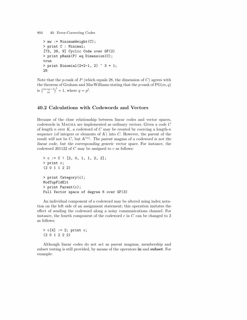
804 40. Error-Correcting Codes
> mw := MinimumWeight(C);> print C : Minimal;[73, 28, 9] Cyclic Code over GF(2)> print pRank(P) eq Dimension(C);true> print Binomial(2+2-1, 2) ^ 3 + 1;28
Note that the p-rank of P (which equals 28, the dimension of C) agrees withthe theorem of Graham and MacWilliams stating that the p-rank of PG(m, q)is
(m+p−1
m
)t+ 1, where q = pt.
40.2 Calculations with Codewords and Vectors
Because of the close relationship between linear codes and vector spaces,codewords in Magma are implemented as ordinary vectors. Given a code Cof length n over K, a codeword of C may be created by coercing a length-nsequence (of integers or elements of K) into C. However, the parent of theresult will not be C, but K(n). The parent magma of a codeword is not thelinear code, but the corresponding generic vector space. For instance, thecodeword 201122 of C may be assigned to c as follows:
> c := C ! [2, 0, 1, 1, 2, 2];> print c;(2 0 1 1 2 2)
> print Category(c);ModTupFldElt> print Parent(c);Full Vector space of degree 6 over GF(3)
An individual component of a codeword may be altered using index nota-tion on the left side of an assignment statement; this operation imitates theeffect of sending the codeword along a noisy communications channel. Forinstance, the fourth component of the codeword c in C can be changed to 2as follows:
> c[4] := 2; print c;(2 0 1 2 2 2)
Although linear codes do not act as parent magmas, membership andsubset testing is still provided, by means of the operators in and subset. Forexample:

40.2 Calculations with Codewords and Vectors 805
> print c in C;false
Coercion of a vector (or a sequence representing a vector) into a code is onlyallowed if the vector is a member of the code. If the vector is not a codeword,an error message will be given:
> print C ! c;
>> print C ! c;^
Runtime error in ’!’: Result is not in the given structure
Table 40.1. Coding-theory operations on vectors
Magma Meaning
InnerProduct(u, v) Inner product of vectors u and v
Distance(u, v) Hamming distance between u and v
Weight(u) Hamming weight of u (number of non-zero entries)
Syndrome(u, C) Syndrome of u relative to code C
Support(u) Set of coordinates of u with non-zero entries
Coordinates(C, u) Coordinates of u relative to basis of C (i.e., coor-dinates of vector v in information space such thatvG = u, where G is generator matrix of C)
Table 40.1 lists the functions on vectors that are designed for use in thecontext of linear codes. See also Section 27.4, for the general-purpose opera-tions on vectors.
The function Syndrome(x, C) provides a way to calculate the syndromeof a vector x relative to a linear code C without explicitly having to calculatethe parity check matrix of C first. For instance, the fact that the syndromeof c relative to C is non-zero is another demonstration that the new versionof c is not in the code C:
> print Syndrome(c, C);(2 2 2)
The function Support(v) returns the set of coordinate positions for whicha vector v has non-zero components. It is useful for such tasks as buildingdesigns from codes. For instance, the support of c shows that only its secondentry is zero:

806 40. Error-Correcting Codes
> print Support(c); 1, 3, 4, 5, 6
40.3 General Facts about a Linear Code
Table 40.2. General facts about a linear code
Magma Meaning
Alphabet(C),Field(C) Underlying field K for code C
Length(C) Block length n of [n, k, d] linear code C
Dimension(C) Dimension k of C
MinimumWeight(C),MinimumDistance(C)
Minimum weight d of words in C
StandardForm(C) Returns (i) a code S equivalent to C butin standard form, (i.e., formed from C withthe columns permuted so that the informa-tion columns are columns 1, . . . , k) (ii) iso-morphism f : C → S. There are many suchcodes, but the same one is returned eachtime.
GeneratorMatrix(C) Generator matrix for C
ParityCheckMatrix(C) Parity check matrix for C
InformationSpace(C) k-dimensional vector space of informationvectors for C
InformationSet(C) Length-k sequence giving the numbers ofthe information columns of C (i.e., k lin-early independent columns of the generatormatrix G, such that G is the identity matrixwhen restricted to these columns)
AllInformationSets(C) All possible information sets of C, as asorted sequence whose terms are length-ksequences of indices of linearly independentcolumns
SyndromeSpace(C) (n − k)-dimensional vector space of syn-drome vectors for C
VectorSpace(C) Vector subspace whose basis corresponds tothe rows of the generator matrix for C
AmbientSpace(C) Generic vector space K(n)
Generic(C) Generic [n, n, 1] code containing C
Dual(C) Dual code of C
Table 40.2 (p. 806) lists functions giving general information about acode while Table 40.3 (p. 807) lists tests for properties. In these tables,

40.3 General Facts about a Linear Code 807
Table 40.3. Properties of a linear code
Magma Meaning
IsCyclic(C) true if C is cyclic
IsMDS(C) true if C is maximum-distance separable(i.e., is an [n, k, n− k + 1] code)
IsSelfOrthogonal(C),IsSelfDual(C)
true if C is self-orthogonal
IsWeaklySelfOrthogonal(C),IsWeaklySelfDual(C)
true if C is weakly self-orthogonal
it should be understood that C is an [n, k, d] linear code over the finitefield K. Most of these functions are fairly trivial, with the exception ofMinimumWeight(C); the advanced facilities for weight enumeration arediscussed later in the chapter. There are some additional functions availablefor cyclic codes, as listed in Table 40.6 (p. 811).
For example, suppose that the binary [4, 2, 2] code generated by 1010 and0111 is created in Magma with the following assignment statement:
> lc := LinearCode< GF(2), 4 | [1,0,1,0], [0,1,1,1] >;
While this one-statement code definition is attractively compact, it has theminor disadvantage that the algebraic structures auxiliary to lc are nameless.The functions listed in the table provide a means of accessing these struc-tures. If, for instance, the user wishes to define the vector v = 0001, whichis not in lc but is in the vector space of which lc is a subspace, then theAmbientSpace(C) should be used to obtain this vector space:
> v := AmbientSpace(lc) ! [0, 0, 0, 1];
The access operations are also useful when writing a function whose ar-gument is an arbitrary code. For instance, according to the sphere-packingbound, any q-ary (n,M, 2t + 1) code satisfies
M
(n
0
)+
(n
1
)(q − 1) + · · ·+
(n
t
)(q − 1)t
≤ qn.
If equality is achieved then the code is called perfect. The following functionspherepacking returns the right hand side of this inequality minus the lefthand side, for a given code C. It employs the functions MinimumWeight,Length, and Field, as well as the operator #, which returns the cardinalityof any given code:
To perform this example online, type load "I96c40e1";

808 40. Error-Correcting Codes
> spherepacking := function(C)> q := #Field(C);> n := Length(C);> M := #C;> t := (MinimumWeight(C) - 1) div 2;> return q^n -> M*(&+[ Binomial(n, i)*(q-1)^i : i in [0..t] ]);> end function;
For instance, the following applications of spherepacking to certain standardlinear codes show that Ham(3, 2) is perfect (as are all the Hamming codesHam(r, q)), but that the extended binary Golay code is far from attainingthe sphere-packing bound:
> print spherepacking(HammingCode(GF(2), 3));0> print spherepacking(GolayCode(GF(2), true));7254016
The generators of a code C are stored in echelonized form, which maydiffer from the way in which they were given by the user. As usual, C.ireturns the ith generator, and Generators(C) returns the generators in aset. Another function, GeneratorMatrix(C), returns a matrix whose rowsare the generators. For example:
> g := GeneratorMatrix(lc);> print g;[1 0 1 0][0 1 1 1]> h := ParityCheckMatrix(lc);> print h;[1 0 1 1][0 1 0 1]> print g * Transpose(h);[0 0][0 0]
40.4 Families of Linear Codes
Magma has functions which return many of the well-known linear codes:Hamming, Reed-Muller, Golay, Reed-Solomon, cyclic, alternant, and gener-alized BCH. For all of these well-known codes, it is much more efficient to

40.4 Families of Linear Codes 809
define them using their special functions rather than specifying their gener-ators by hand.
40.4.1 Some Standard Codes
Table 40.4. Some basic linear codes
Magma Meaning
HammingCode(K, r) [(qr−1)/(q−1), (qr−1)/(q−1)−r, 3] Hammingcode over K
ReedMullerCode(r, m) rth order binary Reed-Muller code of length 2m
(r ≤ m)
GolayCode(K, true) Extended Golay code; binary or ternary ac-cording as K is GF(2) or GF(3)
GolayCode(K, false) Unextended Golay code; binary or ternary ac-cording as K is GF(2) or GF(3)
ReedSolomonCode(K, d) [q − 1, q − d, d] Reed-Solomon code over K
ReedSolomonCode(n, d) As above, where q = n + 1
ReedSolomonCode(K, d, b) [q − 1, q − d, d] Reed-Solomon code over K,where the primitive element is first raised tothe bth power
ReedSolomonCode(n, d, b) As above, where q = n + 1
GRSCode(A, V, k) [n, k′ ≤ k] generalized Reed-Solomon code overK, where A is a sequence of n distinct elementsαi of K, V is a sequence of n non-zero elementsvi of K, and k ≥ 0
Table 40.4 (p. 809) summarizes the functions which return some of thebasic linear codes. In the table, q denotes the cardinality of the field K.
For example, the extended ternary Golay code is created by the assign-ment statement:
> gol3ext := GolayCode(GF(3), true);> print gol3ext;[12, 6, 6] Extended Golay Code over GF(3)Generator matrix:[1 0 0 0 0 0 0 1 1 1 1 1][0 1 0 0 0 0 1 0 1 2 2 1][0 0 1 0 0 0 1 1 0 1 2 2][0 0 0 1 0 0 1 2 1 0 1 2][0 0 0 0 1 0 1 2 2 1 0 1][0 0 0 0 0 1 1 1 2 2 1 0]

810 40. Error-Correcting Codes
40.4.2 Cyclic Codes
Table 40.5. Some cyclic codes
Magma Meaning
CyclicCode(u) [n, k] cyclic code generated by the right cyclic shifts
of vector u ∈ K(n)
CyclicCode(n, f) Length-n cyclic code generated by the right cyclicshifts of the vector corresponding to the polynomialf ∈ K[x], where f has degree n−k and divides xn−1
CyclicCode(n, R, K) Length-n cyclic code over K generated by the least-degree polynomial having the elements of R as roots,where R is a set or sequence of primitive nth rootsof unity in an extension of K
BCHCode(K, n, d, b) q-ary [n, k ≥ n−m(d−1), D ≥ d] BCH code of desig-nated distance d having generator polynomial g(x) =lcmm1(x), . . . , md−1(x), where mi(x) is the mini-
mum polynomial of αb+i−1, for i = 1, . . . , d−1; hereb is a positive integer, α is a primitive nth root ofunity in the degree-m extension of K (i.e., GF(qm)),and n must satisfy gcd(n, q) = 1
BCHCode(K, n, d) As above but with b = 1
QRCode(K, n) q-ary length-n quadratic residue code with generatorpolynomial g0(x) =
Q(x−αr), where α is a primitive
nth root of unity in an extension field L of K, andthe product is taken over the quadratic residues inL; here n is an odd prime such that q is a quadraticresidue modulo n
Table 40.5 (p. 810) lists the functions for the creation of cyclic codes. Onceagain, q denotes the cardinality of the field K. The special operations on cycliccodes are given in Table 40.6 (p. 811); they may be applied to any code whichis cyclic, not only those generated from the functions in Table 40.5.
For example, the length-7 binary cyclic code generated by the vector1101000 corresponding to the polynomial 1 + x + x3 can be generated in anyof the following ways:
> P<x> := PolynomialRing(GF(2));> cyc := CyclicCode(7, 1+x+x^3);> print cyc;[7, 4, 3] Cyclic Code over GF(2)Generator matrix:[1 0 0 0 1 1 0][0 1 0 0 0 1 1]

40.4 Families of Linear Codes 811
Table 40.6. Operations on cyclic codes
Magma Meaning
GeneratorPolynomial(C) A generator polynomial for cyclic code C
CheckPolynomial(C) A check polynomial for cyclic code C
Idempotent(C) Idempotent for cyclic code C
[0 0 1 0 1 1 1][0 0 0 1 1 0 1]
> v := VectorSpace(GF(2), 7) ! [1,1,0,1,0,0,0];> cyc2 := CyclicCode(v);> print cyc2 eq cyc;true
> L<w> := GF(2, 3);> cyc3 := CyclicCode(7, w, w^2, w^4, GF(2));> print cyc3 eq cyc;true
As another example, the length-15 binary BCH code with b = 1 which is2-error-correcting and hence has designated distance 5 is
> BCH15 := BCHCode(GF(2), 15, 5);> print BCH15;[15, 7, 5] BCH code (d = 5, b = 1) over GF(2)Generator matrix:[1 0 0 0 0 0 0 1 0 0 0 1 0 1 1][0 1 0 0 0 0 0 1 1 0 0 1 1 1 0][0 0 1 0 0 0 0 0 1 1 0 0 1 1 1][0 0 0 1 0 0 0 1 0 1 1 1 0 0 0][0 0 0 0 1 0 0 0 1 0 1 1 1 0 0][0 0 0 0 0 1 0 0 0 1 0 1 1 1 0][0 0 0 0 0 0 1 0 0 0 1 0 1 1 1]
40.4.3 Alternant and Generalized BCH Codes
Magma provides several functions for alternant and generalized BCH codes.Some of them are discussed below; in all these descriptions, K = GF(q), andF = GF(qm) is a degree-m extension of K. For more advanced codes, see theHandbook.

812 40. Error-Correcting Codes
Let A and Y be length-n sequences of elements of F , such that the termsof A are distinct and 0 /∈ Y . Then the function AlternantCode(A, Y, r)returns the q-ary [n, k ≥ n−mr, d ≥ r + 1] alternant code A(A, Y ).
Let P and G be univariate polynomials over the splitting field of thepolynomial (xn − 1) over K, such that deg(P ) ≤ n− 1, deg(G) ≤ n− 1, andP and G are coprime to (xn−1). The function ChienChoyCode(P, G, n, q)returns the Chien-Choy generalized BCH code of length n associated with Pand G over GF(q), where gcd(n, q) = 1.
Let G = G(z) be a degree-r polynomial over F . Then GoppaCode(L,G)returns the q-ary [n, k ≥ n − mr, d ≥ r + 1] Goppa code Γ (L,G), whereL = [α1, . . . , αn] is a sequence of n distinct elements of F such that G(αi) 6=0,∀αi ∈ L.
The function SrivastavaCode(A, W,mu,K) returns the Srivastava codeof parameters A,W,mu over K, where mu is an integer and A and W are se-quences of elements of F such that 0 /∈ A and the terms of A and W combinedare distinct. Similarly, GeneralizedSrivastavaCode(A,W,Z, t,K) returnsthe generalized Srivastava code of parameters A,W,Z, t over K, where t > 0and A,W,Z are sequences of elements of F such that 0 /∈ A, 0 /∈ Z, and theterms of A and W combined are distinct.
The following examples illustrate the construction of a Goppa code andan alternant code:
> q := 2^5;> K<w> := GF(q);> Pq<z> := PolynomialRing(K);> G := z^3 + z + 1;> L := [w^i: i in [0..(q-2)]];> print GoppaCode(L, G);[31, 16, 7] Goppa code (r = 3) over GF(2)Generator matrix:[1 0 0 0 0 0 0 0 0 0 0 0 0 0 1 0 1 0 0 1 0 0 1 0 1 1 0 0 0 0 1][0 1 0 0 0 0 0 0 0 0 0 0 0 1 0 0 1 0 0 1 1 1 1 0 0 1 0 1 1 0 1][0 0 1 0 0 0 0 0 0 0 0 0 0 1 0 0 1 0 0 0 1 0 0 1 0 1 0 0 0 0 1][0 0 0 1 0 0 0 0 0 0 0 0 0 1 1 0 0 0 0 1 1 1 0 1 0 1 0 1 0 1 1][0 0 0 0 1 0 0 0 0 0 0 0 0 1 0 0 0 0 0 0 1 1 0 1 1 0 1 1 1 1 1][0 0 0 0 0 1 0 0 0 0 0 0 0 0 0 0 1 0 0 1 0 0 1 0 1 0 0 1 0 1 0][0 0 0 0 0 0 1 0 0 0 0 0 0 1 0 0 1 0 0 0 1 0 1 0 0 1 1 1 0 1 0][0 0 0 0 0 0 0 1 0 0 0 0 0 0 1 0 0 0 0 0 0 1 1 0 1 0 1 0 0 1 1][0 0 0 0 0 0 0 0 1 0 0 0 0 1 1 0 1 0 0 0 0 0 1 0 1 0 1 0 1 0 0][0 0 0 0 0 0 0 0 0 1 0 0 0 0 0 0 0 0 0 1 1 1 1 0 1 1 1 1 0 1 0][0 0 0 0 0 0 0 0 0 0 1 0 0 0 1 0 1 0 0 0 0 0 1 1 1 1 0 1 1 1 1][0 0 0 0 0 0 0 0 0 0 0 1 0 1 1 0 0 0 0 1 1 1 1 0 0 0 1 0 1 1 1][0 0 0 0 0 0 0 0 0 0 0 0 1 0 0 0 1 0 0 1 0 1 0 1 1 0 0 1 1 1 1][0 0 0 0 0 0 0 0 0 0 0 0 0 0 0 1 1 0 0 1 1 1 0 1 0 0 1 1 0 1 0][0 0 0 0 0 0 0 0 0 0 0 0 0 0 0 0 0 1 0 1 1 0 1 0 0 0 1 1 0 0 1][0 0 0 0 0 0 0 0 0 0 0 0 0 0 0 0 0 0 1 0 1 0 0 1 0 1 0 1 1 1 1]

40.5 Constructing Codes from Other Codes 813
> K<u> := GF(4); F := ext< K | 3 >;> n := 15;> w := PrimitiveElement(F);> A := [ w^i : i in [0..n-1] ];> y := [ F!1 : i in [0..n-1] ];> T := AlternantCode(A, y, 4, K);> print T;[15, 5, 7] Alternant code over GF(2^2)Generator matrix:[ 1 0 0 0 0 u 1 u u^2 1 u^2 u u^2 0 0][ 0 1 0 0 0 0 u 1 u u^2 1 u^2 u u^2 0][ 0 0 1 0 0 0 0 u 1 u u^2 1 u^2 u u^2][ 0 0 0 1 0 u^2 0 u u 0 u^2 u^2 u^2 1 0][ 0 0 0 0 1 0 u^2 0 u u 0 u^2 u^2 u^2 1]
40.5 Constructing Codes from Other Codes
There are many ways of constructing a new code by modifying the words ofan existing code in some way. One of these is to build a subcode, with theusual sub constructor. In addition, Magma has functions corresponding tothe constructions specific to coding theory. Table 40.7 (p. 814) summarizesthese functions; in the table, C should be understood to be an [n, k, d] linearcode.
For binary codes, one important characteristic of a codeword is its parity,that is, whether its weight is odd or even. Even-weight codewords are partic-ularly important because any linear combination of such words is also even.Given a binary linear code C, the function ExpurgateCode(C) returns thecode which contains only those codewords of C which are even. For example,in the code h4exp constructed below, every word is even.
> h4 := HammingCode(GF(2), 4);> print h4;[15, 11, 3] Hamming code (r = 4) over GF(2)Generator matrix:[1 0 0 0 0 0 0 0 0 0 0 0 0 1 1][0 1 0 0 0 0 0 0 0 0 0 0 1 1 0][0 0 1 0 0 0 0 0 0 0 0 0 1 0 1][0 0 0 1 0 0 0 0 0 0 1 0 1 1 1][0 0 0 0 1 0 0 0 0 0 1 0 1 0 0][0 0 0 0 0 1 0 0 0 0 1 0 0 1 0][0 0 0 0 0 0 1 0 0 0 1 0 0 0 1][0 0 0 0 0 0 0 1 0 0 1 0 1 1 0][0 0 0 0 0 0 0 0 1 0 1 0 1 0 1][0 0 0 0 0 0 0 0 0 1 1 0 0 1 1]
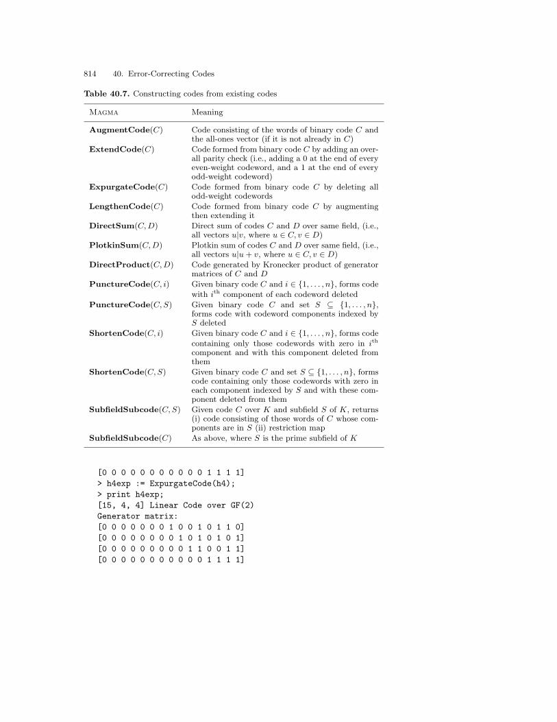
814 40. Error-Correcting Codes
Table 40.7. Constructing codes from existing codes
Magma Meaning
AugmentCode(C) Code consisting of the words of binary code C andthe all-ones vector (if it is not already in C)
ExtendCode(C) Code formed from binary code C by adding an over-all parity check (i.e., adding a 0 at the end of everyeven-weight codeword, and a 1 at the end of everyodd-weight codeword)
ExpurgateCode(C) Code formed from binary code C by deleting allodd-weight codewords
LengthenCode(C) Code formed from binary code C by augmentingthen extending it
DirectSum(C, D) Direct sum of codes C and D over same field, (i.e.,all vectors u|v, where u ∈ C, v ∈ D)
PlotkinSum(C, D) Plotkin sum of codes C and D over same field, (i.e.,all vectors u|u + v, where u ∈ C, v ∈ D)
DirectProduct(C, D) Code generated by Kronecker product of generatormatrices of C and D
PunctureCode(C, i) Given binary code C and i ∈ 1, . . . , n, forms codewith ith component of each codeword deleted
PunctureCode(C, S) Given binary code C and set S ⊆ 1, . . . , n,forms code with codeword components indexed byS deleted
ShortenCode(C, i) Given binary code C and i ∈ 1, . . . , n, forms code
containing only those codewords with zero in ith
component and with this component deleted fromthem
ShortenCode(C, S) Given binary code C and set S ⊆ 1, . . . , n, formscode containing only those codewords with zero ineach component indexed by S and with these com-ponent deleted from them
SubfieldSubcode(C, S) Given code C over K and subfield S of K, returns(i) code consisting of those words of C whose com-ponents are in S (ii) restriction map
SubfieldSubcode(C) As above, where S is the prime subfield of K
[0 0 0 0 0 0 0 0 0 0 0 1 1 1 1]> h4exp := ExpurgateCode(h4);> print h4exp;[15, 4, 4] Linear Code over GF(2)Generator matrix:[0 0 0 0 0 0 0 1 0 0 1 0 1 1 0][0 0 0 0 0 0 0 0 1 0 1 0 1 0 1][0 0 0 0 0 0 0 0 0 1 1 0 0 1 1][0 0 0 0 0 0 0 0 0 0 0 1 1 1 1]

40.5 Constructing Codes from Other Codes 815
Another way of constructing a code in which every word is even is to useall the words of the given code but to modify them so that they are even.The ExtendCode(C) function does this, by extending each word with aparity-check digit. If the minimum weight d is odd, the new code will be an[n + 1, k, d + 1] code. For example:
> h4ext := ExtendCode(h4);> print h4ext;[16, 11, 4] Linear Code over GF(2)Generator matrix:[1 0 0 0 0 0 0 0 0 0 0 0 0 1 1 1][0 1 0 0 0 0 0 0 0 0 0 0 1 1 0 1][0 0 1 0 0 0 0 0 0 0 0 0 1 0 1 1][0 0 0 1 0 0 0 0 0 0 1 0 1 1 1 1][0 0 0 0 1 0 0 0 0 0 1 0 1 0 0 1][0 0 0 0 0 1 0 0 0 0 1 0 0 1 0 1][0 0 0 0 0 0 1 0 0 0 1 0 0 0 1 1][0 0 0 0 0 0 0 1 0 0 1 0 1 1 0 0][0 0 0 0 0 0 0 0 1 0 1 0 1 0 1 0][0 0 0 0 0 0 0 0 0 1 1 0 0 1 1 0][0 0 0 0 0 0 0 0 0 0 0 1 1 1 1 0]
Note that the generator matrix for h4ext is the same as the one for h4 ,except that a column has been added on the right so as to give each generatorcodeword even parity.
If a binary linear code C does not contain the all-ones vector then thefunction AugmentCode(C) will return a larger linear code which containsC, by including the all-ones vector with the words of C. Every binary Ham-ming code contains the all-ones vector of the relevant length already, so thisfunction would merely return h4 itself if applied to h4 , but the dual of h4will give a more fruitful result:
> dualh4 := Dual(h4);> print dualh4;[15, 4, 8] Linear Code over GF(2)Generator matrix:[1 0 1 0 1 1 0 0 1 1 0 0 1 1 0][0 1 1 0 0 1 1 0 0 1 1 1 1 0 0][0 0 0 1 1 1 1 0 0 0 0 1 1 1 1][0 0 0 0 0 0 0 1 1 1 1 1 1 1 1]> dualh4aug := AugmentCode(dualh4);> print dualh4aug;[15, 5, 7] Linear Code over GF(2)Generator matrix:

816 40. Error-Correcting Codes
[1 0 0 0 0 1 1 0 0 1 1 0 0 1 1][0 1 0 0 1 1 0 0 1 1 0 1 0 0 1][0 0 1 0 1 0 1 0 1 0 1 0 1 0 1][0 0 0 1 1 1 1 0 0 0 0 1 1 1 1][0 0 0 0 0 0 0 1 1 1 1 1 1 1 1]> print dualh4 subset dualh4aug;true
The last line above confirms that dualh4 is a subcode of dualh4aug .
The LengthenCode(C) function does two of the above operations in onestep: it first augments C with the all-ones vector and then extends the newcode with a parity-check. This may be tested as follows:
> print LengthenCode(dualh4) eq ExtendCode(dualh4aug);true
There are two functions which return a code which is the sum, either director Plotkin, of two codes C and D. A general codeword in DirectSum(C, D)has the form u|v, and a general codeword in PlotkinSum(C, D) has the formu|u + v, where u ∈ C, v ∈ D. For example, the construction of a first-orderbinary Reed-Muller code can be achieved with Plotkin sums. Since the binaryrepetition codes of lengths 4, 8, and 16 are required in the construction, itis useful to construct a function that returns the binary repetition code ofgiven length n:
To perform this example online, type load "I96c40e2";
> repet := function(n)> allones := [ GF(2)!1 : i in [1..n] ];> return LinearCode(sub<VectorSpace(GF(2), n) | allones>);> end function;
The Reed-Muller code is built by forming the Plotkin sum of the binarylength-4 even-weight code with the binary length-4 repetition code (which,conveniently, are dual to one another), and then by Plotkin summing theresult with the length-8 repetition code, and finally Plotkin summing thisresult with the length-16 repetition code:
> E := PlotkinSum(Dual(repet(4)), repet(4));> F := PlotkinSum(E, repet(8));> G := PlotkinSum(F, repet(16));> print G eq ReedMullerCode(1, 5);true

40.5 Constructing Codes from Other Codes 817
The output verifies that G is the first-order binary Reed-Muller code withm = 5.
There are also some functions which construct new codes according toproperties of individual components of codewords. PunctureCode(C, i)deletes the ith component of each codeword of C to form a new code. Forinstance, the extended binary Golay code, punctured in the ninth position,can be created as follows:
> punct9 := PunctureCode(GolayCode(GF(2), true), 9);
It can be proved that punct9 is equivalent to the unextended binary Golaycode, as is the extended binary Golay code punctured in any other position.However, if they are tested for equality, then the result is false, becauseMagma’s operator eq tests genuine equality, which is a stronger relationshipthan equivalence. A test of equivalence could be performed with the functionIsIsomorphic, explained in Section 40.7.2:
> gol2unext := GolayCode(GF(2), false);> print punct9 eq gol2unext;false
> print IsIsomorphic(punct9, gol2unext);trueMapping from: Code: punct9 to Code: gol2unext
The result indicates that the codes are isomorphic, and also returns the iso-morphism, as a mapping.
The puncturing operation can also be performed on more than one coor-dinate, so there is an alternative form of the function, PunctureCode(C,S),where S is the set of component coordinates to be deleted.
The ShortenCode(C, i) function differs from PunctureCode in thatonly the codewords which have a zero in the ith component are selectedfor the new code. Then these codewords have this component deleted. If acode is to be shortened in several components then the appropriate func-tion is ShortenCode(C,S), where S is the set of components. For instance,Ham(2, 11) may be shortened in the first and second positions:
> h11 := HammingCode(GF(11), 2);> print h11;[12, 10] Hamming code (r = 2) over GF(11)Generator matrix:[ 1 0 0 0 0 0 0 0 0 0 9 2][ 0 1 0 0 0 0 0 0 0 0 9 1]

818 40. Error-Correcting Codes
[ 0 0 1 0 0 0 0 0 0 0 7 3][ 0 0 0 1 0 0 0 0 0 0 3 7][ 0 0 0 0 1 0 0 0 0 0 6 4][ 0 0 0 0 0 1 0 0 0 0 1 9][ 0 0 0 0 0 0 1 0 0 0 2 8][ 0 0 0 0 0 0 0 1 0 0 4 6][ 0 0 0 0 0 0 0 0 1 0 8 2][ 0 0 0 0 0 0 0 0 0 1 5 5]> print ShortenCode(h11, 1, 2);[10, 8] Linear Code over GF(11)Generator matrix:[ 1 0 0 0 0 0 0 0 7 3][ 0 1 0 0 0 0 0 0 3 7][ 0 0 1 0 0 0 0 0 6 4][ 0 0 0 1 0 0 0 0 1 9][ 0 0 0 0 1 0 0 0 2 8][ 0 0 0 0 0 1 0 0 4 6][ 0 0 0 0 0 0 1 0 8 2][ 0 0 0 0 0 0 0 1 5 5]
40.6 The Weight Distribution
The most important invariant of a code C is its minimum distance. In a linearcode, this corresponds to the minimum weight of the codewords of C, wherethe (Hamming) weight of a codeword is defined as the number of non-zerocomponents. Table 40.8 (p. 819) lists some of Magma’s functions connectedwith minimum weight and weight distribution in a code. It should be notedthat the determination of the minimum weight is, in general, a very expensivecomputation, although it can be performed without enumerating the words ofthe code. However, a more efficient algorithm exists for cyclic codes, so in thatcase significantly larger codes can be handled. For the determination of thecomplete weight distribution, it is necessary to enumerate all the codewordsup to scalar multiples. Hence this calculation is much more expensive thanthat of finding the minimum weight.
The function WeightDistribution(C) may be used to determine thenumber of codewords of C of each weight. It returns a sequence of tuples,each of which is an integer pair such that the first number is a ith weightand the second number is the number of codewords with that weight. Forexample:
> print WeightDistribution(C);[ <0, 1>, <3, 6>, <4, 12>, <5, 6>, <6, 2> ]

40.6 The Weight Distribution 819
Table 40.8. Weight distribution functions
Magma Meaning
CoveringRadius(C) Covering radius of C
Diameter(C) Largest weight of words of C
MinimumWeight(C),MinimumDistance(C)
Minimum weight d of words in C
Weight(u) Weight of vector u
MinimumWords(C) Set of words of C having minimumweight
Words(C, t) Set of words of C with weight t
NumberOfWords(C, t) Number of words of C with weight t
WeightDistribution(C) Sequence of tuples <wi, ni> where ni
is the number of codewords of C withweight wi (ni > 0)
WeightDistribution(C, u) Weight distribution of coset C + u,giving weight-counts of coset vec-tors (as a sequence of form describedabove)
CosetDistanceDistribution(C) Sequence of tuples <di, ni> where ni
is the number of cosets of C with dis-tance di from C (ni > 0)
DualWeightDistribution(C) Weight distribution of dual of C
MacWilliamsTransform(n, k, q, W ) Supposing a hypothetical [n, k] codeC over GF(q), with weight distribu-tion W , return weight distribution ofdual of C
> print WeightDistribution(h4);[ <0, 1>, <3, 35>, <4, 105>, <5, 168>, <6, 280>, <7, 435>,<8, 435>, <9, 280>, <10, 168>, <11, 105>, <12, 35>,<15, 1> ]
The other Magma functions associated with weight distribution, includingMacWilliamsTransform, express the distribution in the same form.
Information about weight distribution may be obtained in a different formfrom the function WeightEnumerator(C). It returns an integer polynomialin two indeterminates, x and y say, such that the coefficient of xiyn−i isthe number of codewords with weight i. There are two methods for namingthe indeterminates (i.e., as identifiers and as printnames): either by creat-ing the parent ring over the integers with generator assignment or by usinggenerator assignment while assigning the polynomial. Both techniques aredemonstrated below, so that the user may choose whichever is preferred:
> print WeightEnumerator(C);

820 40. Error-Correcting Codes
Table 40.9. Weight enumerator functions
Magma Meaning
WeightEnumerator(C) Polynomial in two indeterminates inwhich coefficient of xiyn−i is numberof codewords of C with weight i
WeightEnumerator(C, u) Weight enumerator of coset C + u,giving weight-counts of coset vectorsas a polynomial (of form describedabove)
CompleteWeightEnumerator(C) Complete weight enumerator of Cover GF(q), as a polynomial in qindeterminates
CompleteWeightEnumerator(C, u) Complete weight enumerator of cosetC + u
MacWilliamsTransform(n, k, K, W ) Supposing a hypothetical [n, k] codeC over K, with complete weight enu-merator W , return complete weightenumerator of dual of C
$.1^6 + 6*$.1^3*$.2^3 + 12*$.1^2*$.2^4 + 6*$.1*$.2^5+ 2*$.2^6
> // 1st method> P<x,y> := PolynomialRing(IntegerRing(), 2);> print WeightEnumerator(C);x^6 + 6*x^3*y^3 + 12*x^2*y^4 + 6*x*y^5 + 2*y^6
> // 2nd method> wtenum<x,y> := WeightEnumerator(C);> print wtenum;x^6 + 6*x^3*y^3 + 12*x^2*y^4 + 6*x*y^5 + 2*y^6
The weight enumerator functions are listed in Table 40.9 (p. 820).
40.7 Group Actions, Automorphism and Equivalence
40.7.1 Group Actions on Codes
There are two kinds of group action on an [n, k] linear code C over GF(q):permutation action and monomial action. If G is a permutation group of de-gree n, then the permutation action of g ∈ G on C is the operation whereby

40.7 Group Actions, Automorphism and Equivalence 821
the coordinate positions of codewords are permuted according to the permu-tation g. If G is a permutation group of degree n(q − 1), then the monomialaction of g ∈ G on C is the operation whereby not only coordinate positionsare permuted, but also the coordinatees are multiplied by a non-zero elementof GF(q). (Only some of the elements of G describe monomial permutations.)Note that if C is a binary code (q = 2), then monomial action reduces topermutation action.
[In more detail, a monomial permutation of monomial degree n is essen-tially a permutation s on the Cartesian product of the non-zero elements ofK and the set S = 1, . . . , n which satisfies the following property for allnon-zero α, β, γ ∈ K and i, j,∈ S:
(α, i)s = (β, j) implies (γα, i)s = (γβ, j).
Note that s is completely determined by its action on the points (1, i) foreach i; note also that the actual degree of s is (q − 1)n. To represent amonomial permutation of monomial degree n, we number the pair (α, i) by(q − 1)(i− 1) + α and then use a permutation s of degree (q − 1)n.]
The Magma operator ^ or the function Image may be used to computeimages of codewords under group actions. Suppose that c is a codeword (orindeed any vector) with n coordinates over GF(q), and that g is an elementof a permutation group G over the standard support. If the degree of G is n,then the expression c^g or Image(g, c) returns the vector which is the imageof c under the permutation action of g. On the other hand, if the degree of Gis n(q−1), and g describes a monomial permutation, then c^g or Image(g, c)returns the vector which is the image of c under the monomial action of g. Ifthe degree of G is neither n nor n(q−1), then an error message will be given.
For example, let gol3ext be the extended ternary Golay code. The follow-ing lines show how to find the images of the sixth generator of gol3ext undera certain permutation action and monomial action. It emerges that neitherof the images are in the code:
> gol3ext := GolayCode(GF(3), true);> gen6 := gol3ext.6; print gen6;(0 0 0 0 0 1 1 1 2 2 1 0)> g1 := Sym(12) ! (5, 6, 7)(1, 10);> v1 := gen6 ^ g1; // permutation action> print v1;(2 0 0 0 1 0 1 1 2 0 1 0)> g2 := Sym(24) ! (5, 7)(6, 8)(11, 16, 20)(12, 15, 19);> v2 := gen6 ^ g2; // monomial action> print v2;(0 0 0 0 0 1 1 2 2 1 1 0)> print v1 in gol3ext, v2 in gol3ext;

822 40. Error-Correcting Codes
false false
Group actions on a code C (or vector space) are computed by findingthe action on the generators of C and returning the code generated by theresulting images. Both permutation and monomial actions may be computed,as for single codewords. The image of C under a permutation action is iso-morphic to C, and the image of C under a monomial action is equivalent toC. For instance, the code isoC created below is isomorphic to gol3ext :
> isoC := gol3ext ^ g1; print isoC;[12, 6, 6] Linear Code over GF(3)Generator matrix:[1 0 0 0 0 0 0 1 1 1 1 1][0 1 0 0 0 0 2 2 2 0 1 1][0 0 1 0 0 0 2 1 2 1 2 0][0 0 0 1 0 0 2 0 1 2 2 1][0 0 0 0 1 0 1 2 0 1 2 1][0 0 0 0 0 1 2 2 1 1 0 2]
The column-relationship between isoC and gol3ext is not obvious to theeye, because when Magma creates a vector space or code, it echelonizes thegenerators to find a basis. The following calculations show in more detail theunderlying process:
> new_gens := [gol3ext.i ^ g1 : i in [1..6]];> new_code := LinearCode< GF(3), 12 | new_gens >;> print new_code eq isoC;true
Whenever an object is acted on by a permutation group rather than asingle permutation, the result is the G-set of the images of the object undereach permutation in the group. Among the possible objects are a vector anda code. For example, consider the dihedral group of degree 12 and order 24in its action on the first generator of gol3ext :
> print gol3ext.1 ^ DihedralGroup(12);GSet
(1 0 0 0 0 0 0 1 1 1 1 1),(0 0 0 1 1 1 1 1 1 0 0 0),(1 1 1 1 1 0 0 0 0 0 0 1),(1 1 0 0 0 0 0 0 1 1 1 1),(0 0 0 0 1 1 1 1 1 1 0 0),(1 1 1 1 1 1 0 0 0 0 0 0),(1 1 1 1 0 0 0 0 0 0 1 1),(0 0 1 1 1 1 1 1 0 0 0 0),

40.7 Group Actions, Automorphism and Equivalence 823
(0 0 0 0 0 0 1 1 1 1 1 1),(1 1 1 0 0 0 0 0 0 1 1 1),(0 0 0 0 0 1 1 1 1 1 1 0),(0 1 1 1 1 1 1 0 0 0 0 0)
Since the size of this G-set is less than the order of the group, not all of theimages are distinct.
For details of other permutation group operations, see Chapter 32. Thereis one more group action function specially tailored for codes: given an [n, k]code C and a permutation group G of degree n, Fix(C, G) returns the sub-code of C consisting of the codewords that are fixed by the elements of G.
40.7.2 Equivalent and Isomorphic Codes
Two linear codes in K(n) are equivalent if one may be obtained from theother by a monomial action. The function IsEquivalent(C,D) tests whetherthe codes C and D are equivalent. If they are equivalent, it returns thecorresponding mapping from C to D as a second value. For example,
> C1 := LinearCode<GF(3), 3 | [1,0,1]>;> C2 := LinearCode<GF(3), 3 | [1,2,0]>;> i, f := IsEquivalent(C1, C2);> print i;true> print f(C1) eq C2;true
Two linear codes in K(n) are isomorphic if one may be obtained from theother by a permutation action, that is, by permuting the columns (coordinatepositions). For binary codes, this is the same as equivalence, but for othercodes, isomorphism is a stronger relationship than equivalence. Currently,isomorphism testing is only possible in Magma for binary codes. The functionIsIsomorphic(C, D) tests whether the binary codes C and D are isomorphic;if the principal return value is true, it returns as a second value a mappingwhich is an isomorphism from C to D.
As an example, consider the first-order binary Reed-Muller code R withm = 4, and the code T formed by the action of p = (4, 13)(5, 12)(6, 11) underR. The following lines demonstrate that R and T are isomorphic, as expected:
> R := ReedMullerCode(1, 4); print R;[16, 5, 8] Reed-Muller Code (r = 1, m = 4) over GF(2)

824 40. Error-Correcting Codes
Generator matrix:[1 0 0 1 0 1 1 0 0 1 1 0 1 0 0 1][0 1 0 1 0 1 0 1 0 1 0 1 0 1 0 1][0 0 1 1 0 0 1 1 0 0 1 1 0 0 1 1][0 0 0 0 1 1 1 1 0 0 0 0 1 1 1 1][0 0 0 0 0 0 0 0 1 1 1 1 1 1 1 1]> p := Sym(16) ! (4, 13)(5, 12)(6, 11);> T := R ^ p; print T;[16, 5, 8] Linear Code over GF(2)Generator matrix:[1 0 0 0 0 1 0 1 0 1 0 1 1 1 1 0][0 1 0 0 0 1 1 0 1 0 0 1 1 1 0 1][0 0 1 0 0 0 0 0 1 1 1 1 1 0 1 1][0 0 0 1 0 0 1 1 0 0 1 1 0 1 1 1][0 0 0 0 1 1 1 1 1 1 1 1 0 0 0 0]> print R eq T;false> iso, m := IsIsomorphic(R, T);> print iso, m;true Mapping from: Code: R to Code: T
Note that isomorphic codes need not have the same standard form. Thefunction StandardForm(C), explained in Table 40.7 (p. 814), returns a codein standard form that is isomorphic to C. It returns the same code every time,but there are actually many codes satisfying the description. For example:
> print StandardForm(R) eq StandardForm(T);false
The functions IsEquivalent(C,D) and IsIsomorphic(C, D) both have aparameter AutomorphismGroups which can take any of the string values"None", "Left", "Right" (the default), or "Both". It specifies which, if any,of the automorphism groups of the codes (see below) are to be constructedfirst. For certain examples, the isomorphism test progresses faster when thisparameter is changed from its default value.
40.7.3 Automorphism Groups
Magma offers facilities for computing the automorphism groups correspond-ing to each kind of group action on a code. Given an [n, k] code C overGF(q), the function MonomialGroup(C) or AutomorphismGroup(C)returns the group of all monomial transformations that preserve C, as a per-mutation group of degree n(q − 1). The function PermutationGroup(C)returns the group of coordinate permutations that map the code C into itself,

40.7 Group Actions, Automorphism and Equivalence 825
as a permutation group of degree n. (This group is equal to the monomialautomorphism group only if C is binary.) Each of these functions returnsthree values: the group itself; the parent M for all such automorphisms of Cwhen represented as maps; and a transfer map t from G to M .
For example, let BCHmod11 be the [10, 6, 5] BCH code over GF(11). Thefollowing statements demonstrate the construction of and operations on themonomial group and permutation group of BCHmod11 :
> BCHmod11 := BCHCode(GF(11), 10, 5);> A, Apm, At := MonomialGroup(BCHmod11);> print Apm;Set of all automorphisms of [10, 6, 5] BCH code(d = 5, b = 1) over GF(11)> print At;Mapping from: GrpPerm: A to PowMap: Apm> print A;Permutation group A acting on a set of cardinality 100Order = 200 = 2^3 * 5^2
(1, 11, 10, 20)(2, 12, 9, 19)(3, 13, 8, 18)(4, 14, 7,17)(5, 15, 6, 16)(21, 91, 30, 100)(22, 92, 29,99)(23, 93, 28, 98)(24, 94, 27, 97)(25, 95, 26,96)(31, 90, 40, 81)(32, 89, 39, 82)(33, 88, 38,83)(34, 87, 37, 84)(35, 86, 36, 85)(41, 71, 50,80)(42, 72, 49, 79)(43, 73, 48, 78)(44, 74, 47,77)(45, 75, 46, 76)(51, 70, 60, 61)(52, 69, 59,62)(53, 68, 58, 63)(54, 67, 57, 64)(55, 66, 56,65)
(1, 9, 4, 3, 5)(2, 7, 8, 6, 10)(11, 92, 14, 98, 15,100, 19, 97, 13, 96)(12, 94, 18, 95, 20, 99, 17,93, 16, 91)(21, 89, 24, 83, 25, 81, 29, 84, 23,85)(22, 87, 28, 86, 30, 82, 27, 88, 26, 90)(31,72, 34, 78, 35, 80, 39, 77, 33, 76)(32, 74, 38,75, 40, 79, 37, 73, 36, 71)(41, 69, 44, 63, 45,61, 49, 64, 43, 65)(42, 67, 48, 66, 50, 62, 47,68, 46, 70)(51, 52, 54, 58, 55, 60, 59, 57, 53,56)
(1, 10)(2, 9)(3, 8)(4, 7)(5, 6)(11, 91)(12, 92)(13,93)(14, 94)(15, 95)(16, 96)(17, 97)(18, 98)(19,99)(20, 100)(21, 90)(22, 89)(23, 88)(24, 87)(25,86)(26, 85)(27, 84)(28, 83)(29, 82)(30, 81)(31,71)(32, 72)(33, 73)(34, 74)(35, 75)(36, 76)(37,77)(38, 78)(39, 79)(40, 80)(41, 70)(42, 69)(43,68)(44, 67)(45, 66)(46, 65)(47, 64)(48, 63)(49,62)(50, 61)

826 40. Error-Correcting Codes
(11, 100)(12, 99)(13, 98)(14, 97)(15, 96)(16, 95)(17,94)(18, 93)(19, 92)(20, 91)(21, 81)(22, 82)(23,83)(24, 84)(25, 85)(26, 86)(27, 87)(28, 88)(29,89)(30, 90)(31, 80)(32, 79)(33, 78)(34, 77)(35,76)(36, 75)(37, 74)(38, 73)(39, 72)(40, 71)(41,61)(42, 62)(43, 63)(44, 64)(45, 65)(46, 66)(47,67)(48, 68)(49, 69)(50, 70)(51, 60)(52, 59)(53,58)(54, 57)(55, 56)
> print CompositionFactors(A);G| Cyclic(2)*| Cyclic(2)*| Cyclic(5)*| Cyclic(2)*| Cyclic(5)1
> P, Ppm, Pt := PermutationGroup(BCHmod11);> print P;Permutation group P acting on a set of cardinality 10
(1, 2, 3, 4, 5, 6, 7, 8, 9, 10)> print Ppm;Set of all automorphisms of [10, 6, 5] BCH code(d = 5, b = 1) over GF(11)> print Pt;Mapping from: GrpPerm: P to PowMap: Apm
> c := Random(BCHmod11); print c;( 1 10 5 1 5 9 5 0 1 5)> ga := Random(A); print ga;(1, 37, 6, 39, 3, 40, 7, 35, 9, 38, 10, 34, 5, 32, 8, 31,
4, 36, 2, 33)(11, 24, 16, 22, 13, 21, 17, 26, 19, 23,20, 27, 15, 29, 18, 30, 14, 25, 12, 28)(41, 97, 46,99, 43, 100, 47, 95, 49, 98, 50, 94, 45, 92, 48, 91,44, 96, 42, 93)(51, 84, 56, 82, 53, 81, 57, 86, 59,83, 60, 87, 55, 89, 58, 90, 54, 85, 52, 88)(61, 77,66, 79, 63, 80, 67, 75, 69, 78, 70, 74, 65, 72, 68,71, 64, 76, 62, 73)
> print c ^ ga; // or Image(ga, c)( 4 2 7 7 9 7 0 2 3 2)

40.8 Encoding and Decoding 827
> pa := Random(P); print pa;(1, 8, 5, 2, 9, 6, 3, 10, 7, 4)> print c ^ pa;( 1 5 9 5 0 1 5 1 10 5)
> print Orbit(P, c);GSet
( 0 1 5 1 10 5 1 5 9 5),( 5 9 5 0 1 5 1 10 5 1),(10 5 1 5 9 5 0 1 5 1),( 5 1 5 9 5 0 1 5 1 10),( 1 5 9 5 0 1 5 1 10 5),( 5 0 1 5 1 10 5 1 5 9),( 5 1 10 5 1 5 9 5 0 1),( 1 10 5 1 5 9 5 0 1 5),( 1 5 1 10 5 1 5 9 5 0),( 9 5 0 1 5 1 10 5 1 5)
> print BCHmod11^ga eq BCHmod11;true
The parent M of the automorphism maps and transfer map t can also becreated without calling the AutomorphismGroup(C) function explicitlyby the function Aut(C) which returns M and t. In this case, the domain of t isthe full symmetric group of the appropriate degree (for the monomial action)so an automorphism of I can be applied to by t. The function Aut(C, T )allows one to select the kind of action: if T is ‘‘Monomial’’, the monomialaction is used; if T is ‘‘Permutation’’, the permutation action is used.
40.8 Encoding and Decoding
The original motivation for coding theory was the encoding and decoding ofinformation. This section will demonstrate the concepts involved, and theirassociated functions.
40.8.1 Encoding
Consider the extended binary Hamming code C = Ham(4, 2). This codemay be created in Magma by extending Ham(4, 2) and putting the result instandard form:

828 40. Error-Correcting Codes
> h4 := HammingCode(GF(2), 4);> C := StandardForm(ExtendCode(h4));> print C;[16, 11, 4] Linear Code over GF(2)Generator matrix:[1 0 0 0 0 0 0 0 0 0 0 0 0 1 1 1][0 1 0 0 0 0 0 0 0 0 0 0 1 1 0 1][0 0 1 0 0 0 0 0 0 0 0 0 1 0 1 1][0 0 0 1 0 0 0 0 0 0 0 1 1 1 1 1][0 0 0 0 1 0 0 0 0 0 0 1 1 0 0 1][0 0 0 0 0 1 0 0 0 0 0 1 0 1 0 1][0 0 0 0 0 0 1 0 0 0 0 1 0 0 1 1][0 0 0 0 0 0 0 1 0 0 0 1 1 1 0 0][0 0 0 0 0 0 0 0 1 0 0 1 1 0 1 0][0 0 0 0 0 0 0 0 0 1 0 1 0 1 1 0][0 0 0 0 0 0 0 0 0 0 1 0 1 1 1 0]
Since the code C has length 16 and dimension 11, it encodes messages of 11binary digits into codewords of 16 binary digits. The minimum weight of Cis 4, so it can correct any single error, using nearest-neighbour decoding, anddetect any double error.
Suppose now that the message to be encoded is 01101001101. It may bedefined in Magma as a vector in the information space of C:
> infospace := InformationSpace(C);> message := infospace![0,1,1,0,1,0,0,1,1,0,1];
To encode this vector, it must be multiplied by the generator matrix of C:
> encoded := message * GeneratorMatrix(C);> print encoded;(0 1 1 0 1 0 0 1 1 0 1 1 0 1 1 1)
Observe that encoded is the message vector followed by five check digits. Thisis because the code was created in standard form, in which the informationset corresponds to the first k components of the [n, k] code. This may beverified by typing
> print InformationSet(C);[ 1, 2, 3, 4, 5, 6, 7, 8, 9, 10, 11 ]
to obtain the sequence from 1 to 11 inclusive. (The function returns a se-quence rather than a set because it is often useful for the information set tobe ordered.)

40.8 Encoding and Decoding 829
40.8.2 Errors in Transmission
Now imagine that encoded is sent along a noisy communications channel, andthat consequently an error occurs in the eighth place of the codeword. Thefollowing assignment statements will simulate this:
> received := encoded;> received[8] := 0;
The task of decoding involves the detection and correction of the error inreceived .
40.8.3 Elementary Syndrome-Decoding Techniques
The syndrome of a vector relative to a code is zero if and only if that vectoris a word of the code. A call to the function Syndrome will show that thesyndrome of received is non-zero:
> syn := Syndrome(received, C);> print syn;(0 0 0 0 1)
Therefore received is not a codeword. That is, the presence of error(s) intransmission has been detected.
Syndrome decoding rests on the theorem that two vectors have the samesyndrome if and only if they are in the same coset of the code. The functionCosetLeaders(C) returns a sequence containing all the coset leaders of acode C, and also returns a map from the syndrome space to the ambientspace of the code. It is the map that is needed in this circumstance, becausein practice it returns the coset leader with the given syndrome. The map isapplied to the syndrome in the lines below:
> cl, syntoleader := CosetLeaders(C);> errorvec := syn @ syntoleader;> print errorvec;(0 0 0 0 0 0 0 1 0 0 0 0 0 0 0 0)
The error vector is all zero except for the eighth component, as expected.The received vector must be corrected by subtracting the error vector:
> corrected := received - errorvec;

830 40. Error-Correcting Codes
Now the decoding process is almost complete, since the decoded messagecan be extracted as the information part of corrected , using the functionCoordinates(C, u):
> decoded := infospace ! Coordinates(C, corrected);> print decoded eq message;true
The message has been decoded successfully.
The limitations of a code can also be explored in this way. Suppose thereceived vector has an error in the sixth place as well. In this case, whenthe error vector is calculated using the same method as above, the answer iswrong; it should be 0000010100000000:
> rec2 := received; rec2[6] := 1;
> err2 := Syndrome(rec2, C) @ syntoleader;> print err2;(1 0 0 0 0 0 0 0 0 0 1 0 0 0 0 0)
If the decoding process is continued with this incorrect error vector, then thedecoded vector dec2 will not equal the original message:
> corr2 := rec2 - err2;> dec2 := infospace ! Coordinates(C, corr2);> print dec2;(1 1 1 0 1 1 0 0 1 0 0)
The problem in this second example occurred because rec2 was equally spaced(with a distance of two) between two codewords, corrected and corr2 :
> print Distance(rec2, corrected);2> print Distance(rec2, corr2);2
The decoding procedure regrettably chose the wrong codeword. Here is anexample of a double error which C can detect but not correct.
40.8.4 Automated Decoding
The Magma function Decode performs an automated form of decoding, inthe restricted sense of constructing the corrected vector from the received

40.8 Encoding and Decoding 831
vector as demonstrated above. Two algorithms are accessible: syndrome de-coding, as explained above; and a Euclidean algorithm, which operates onalternant codes (including BCH, Goppa, and Reed-Solomon codes, as well asthose discussed in Section 40.4.3). [The reader should consult the Handbookfor further decoding methods.] The Euclidean algorithm cannot correct asmany errors as the syndrome algorithm can, but in general it is faster, sincethe syndrome algorithm requires the coset leaders of the code. If the codeis alternant, the Euclidean algorithm is used by default, but the user mayrequest the other algorithm by assigning the string "Syndrome" to the param-eter Al instead of the default value "Euclidean". For non-alternant codes,only syndrome decoding is possible, so the parameter Al is not relevant.
Given a code C and a vector v in the ambient space of C, Decode(C, v)attempts to decode v. If the decoding algorithm succeeds in computing avector v′ as the decoded version of v, then Decode returns true and v′. Inthe Euclidean case it may happen that v′ is not in C, so the user shouldtake care. If the decoding algorithm does not succeed in decoding v, thenDecode returns false and the zero vector. This function can also operate ona sequence Q of vectors: Decode(C,Q) returns a sequence of Booleans anda sequence of decoded vectors corresponding to the given sequence.
The statements below illustrate automatic syndrome decoding on a non-alternant code, using the same examples as above. Note that the results arethe same as those achieved through manual application of syndrome decodingtechniques:
> OK, corrD := Decode(C, received);> print OK;true> print corrD eq corrected;true
> OK2, corr2D := Decode(C, rec2);> print OK2;true> print corr2D eq corr2;true
The final phase in decoding, the computation of the information part of thecorrected vector, should be accomplished as demonstrated previously.
The next example demonstrates the application of the Euclidean decodingalgorithm with respect to the [10, 6, 5] BCH code over GF(11):
> BCHmod11 := BCHCode(GF(11), 10, 5);> print BCHmod11;

832 40. Error-Correcting Codes
[10, 6, 5] BCH code (d = 5, b = 1) over GF(11)Generator matrix:[ 1 0 0 0 0 0 1 8 5 3][ 0 1 0 0 0 0 8 10 4 7][ 0 0 1 0 0 0 4 7 8 5][ 0 0 0 1 0 0 6 8 4 4][ 0 0 0 0 1 0 7 7 10 3][ 0 0 0 0 0 1 8 5 3 1]
This code contains 116 codewords and is a subspace of a vector space contain-ing 1110 vectors, so there are 114 coset leaders. By using Euclidean decodingrather than syndrome decoding, the construction of these coset leaders canbe avoided. (On the other hand, the coset leaders of a code are stored oncethey are computed, so it is a once-only time constraint.) For example:
> BCHenc := Random(BCHmod11);> print BCHenc;( 0 0 6 9 10 2 10 7 3 10)> BCHrec := BCHenc; BCHrec[5] := 1; BCHrec[10] := 7;> print BCHrec;( 0 0 6 9 1 2 10 7 3 7)
> // Euclidean decoding> time OK, BCHcorr := Decode(BCHmod11, BCHrec);Time: 0.000> print OK;true> print BCHcorr;( 0 0 6 9 10 2 10 7 3 10)> print BCHcorr eq BCHenc;true> // Syndrome decoding> time OK, BCHcorr := Decode(BCHmod11, BCHrec :> Al := "Syndrome");Time: 11.501> print BCHcorr eq BCHenc;true
For a sequence example, consider the Goppa code defined below. In thiscode, r = 3, so the Euclidean algorithm is able to correct b r
2c = 1 error:
> q := 2^5;> K<w> := GF(q);> Pq<z> := PolynomialRing(K);> G := z^3 + z + 1;

40.8 Encoding and Decoding 833
> L := [w^i: i in [0..(q-2)]];> GC := GoppaCode(L, G);> print GC : Minimal;[31, 16, 7] Goppa code (r = 3) over GF(2)
> wds := [ Random(GC) : i in [1..20] ];> vecs := wds;> for i in [1..20] do> vecs[i, Random(1, 31)] +:= 1;> end for;> OK, rec := Decode(GC, vecs);> print false notin OK;true> print rec eq wds;true
40.8.5 Simulation of Message Transmission
Suppose that str is a message, represented as a string. The function senddeveloped below encodes str using an error-correcting code, imitates thetransmission of the encoded version along a noisy communications channel,optionally applies a decoder to the received version to obtain a corrected ver-sion, and finally converts the corrected version back to a string and returnsthe result.
For simplicity, the string is encoded character-by-character. Therefore, inorder to encode the characters with ASCII codes 1 to 127, a code with atleast 127 codewords is required. The code C chosen for the demonstration isa binary BCH code with n = 15 and d = 5, having 128 codewords, so one ofthe codewords will not be used.
The function send has three arguments: the string str ; a non-negativenumber noise, such that 0 means perfect transmission, slightly higher valuesmean that some codeword components may be altered, and 1 means everycodeword component will be altered; and a Boolean decode, which should beset to true if and only if the Decode algorithm is to be applied. It returns astring of the same length as str , which will resemble it to an extent dependingon the values of noise and decode.
To perform this example online, type load "I96c40e3";
> send := function(str, noise, decode)> C := BCHCode(GF(2), 15, 5);> GM := GeneratorMatrix(C);

834 40. Error-Correcting Codes
> InfSp := InformationSpace(C);> wds := Setseq(Set(InfSp));> STC := StringToCode;> CTS := CodeToString;> // from string to sequence of codewords> enc := [ wds[STC(str[i])] * GM :> i in [1..#str]];>> // introduce noise> perturbate := function(v)> for i := 1 to Length(C) do> if Random(1000) / 1000 le noise then> v[i] := v[i] + 1;> end if;> end for;> return v;> end function;> rec := [ perturbate(v) : v in enc ];>> // apply Decode algorithm if requested> if decode then> _, corr := Decode(C, rec);> else> corr := rec;> end if;>> // convert non-codewords to the codeword for "X"> Xwd := wds[STC("X")] * GM;> corrB := [ v in C select v else Xwd : v in corr ];> // find index-positions for the codewords,> dec := [ Index(wds, InfSp!Coordinates(C, wd)) : wd in corrB ];> // convert the (illegal) index-positions> // of the unused codewords to the index for "x"> xindex := STC("x");> decB := [ i le 127 select i else xindex : i in dec ];>> return &cat[ CTS(i) : i in decB ];> end function;
For example,
> text := "Mathematicians are like Frenchmen: \> whenever you say something to them, \> they translate it into their own language, \> and at once it is something entirely different.

40.9 Advanced Facilities 835
> J. W. von Goethe";> print text;Mathematicians are like Frenchmen: whenever you saysomething to them, they translate it into their ownlanguage, and at once it is something entirely different.
J. W. von Goethe
> print send(text, 0.01, false);MathXmaticians aXe likX XreXcXmen: whenXver you saysXmetXing to theX, they translXte iX into tXeirownXlXnguage, and at once XtXiXsomXthingXentirelyXdifXerXnt.X J. W. von Goethe
> print send(text, 0.01, true);Mathematicians are like Frenchmen: whenever yousayXsomething to them, they translate it into their ownlanguage, and at once it is something entirely different.
J. W. von Goethe> print send(text, 0.1, false);XXXXXXXXXXXXXXXaXXXXXXeXXXXXXXXXXXXXXXXXXXXXXXXXaXXsXXXtXXXgXXXXXXeXX XXeyXXrXnsXaXXiXXXXXXXXhXiXXXwXXXXXXXXXXXXXXXXaXXXXcXXXtXiXXXXXXXXiXXXXXX\XXXXXXXXXXeXeXXXXXX XXXXXX.XXXXXXXXXoeXXe> print send(text, 0.1, true);MatXmatiXians‘areliXe FrencXmen: whenevXX@yousaX7XmethinXto them, theX translate it iN=o shXir ownlnguggeX anD@at once it is something entiXely different.X X J.XW. on GoetXe
40.9 Advanced Facilities
In addition to the operations described in this chapter, Magma contains fur-ther functions for constructing particular families of codes. Access is providedto a database of upper and lower bounds on the minimum distance for anoptimal [n, k] code as tabulated by Brouwer and Sloane for codes over GF(2),GF(3) and GF(4).

836 40. Error-Correcting Codes
40.10 Notes on the Algorithms
The algorithms for computing minimum distances and weight distributionswere developed by Allan Steel from ideas of Andries Brouwer. Testing equiv-alence of codes and the computation of automorphism groups are peformedusing Jeff Leon’s package PERM.

References
[AsK92] Assmus, E. F., Jr. and Key, J. D. (1992). Designs and Their Codes. Cam-bridge: Cambridge University Press.
[BBC93] Batut, C., Bernardi, D., Cohen, H. and Olivier, M. (November 1, 1993).User’s Guide to PARI-GP. Unpublished. Updated for version 1.38.2.
[BeW93] Becker, T. and Weispfenning, V. (1993). Grobner Bases. New York:Springer Verlag.
[Ber71] Berge, B. (1971). Principles of Combinatorics. New York: AcademicPress.
[BGK86] Boege, Gebauer, and Kredel (1986). Some Examples for Solving Systemsof Algebraic Equations by Calculating Groebner Bases. In: J. SymbolicComputation (1986) 1, 83–98.
[Boo59] Boone, W.W. (1959). The word problem. Annals of Math. , 207–265.
[BoC96] Bosma, W. and Cannon, J. J. (1996). Handbook of Magma Functions.Sydney: School of Mathematics and Statistics, University of Sydney.
[BCM94] Bosma, W., Cannon, J. J., Matthews, G. (1994). Programming with alge-braic structures: design of the Magma language. In: M. Giesbrecht (ed.),Proceedings of the 1994 International Symposium on Symbolic and Alge-braic Computation, Oxford, 52–57. Association for Computing Machinery.
[BCP96] Bosma, W., Cannon, J.J., Playoust, C. (1996). The Magma Algebra Sys-tem I: The user language. Submitted to J. Symbolic Computation.
[BCP96] Bosma, W., Cannon, J. J, Playoust, C., Steel, A. (1996). Solving Problemswith Magma. Sydney: School of Mathematics and Statistics, Universityof Sydney.
[Bou70] Bourbaki, N. (Nouvelle Edition 1970). Algebre I: Chapitres 1 a 3
(Elements de Mathematique). Paris: Hermann.

838 References
[BuC89] Butler, G. and Cannon, J. J. (1989). Cayley version 4: The user lan-guage. [The early name for Magma was Cayley V4.] In: P. Gianni (ed.),Proceedings of the 1988 International Symposium on Symbolic and Alge-braic Computation, Rome, July 4–8, 1988, Lecture Notes in ComputerScience 358, 456–466. New York: Springer.
[BuC90] Butler, G. and Cannon, J. J. (1990). The design of Cayley, a languagefor modern algebra. In: A. Miola (ed.), Design and Implementation ofSymbolic Computation Systems, Lecture Notes in Computer Science 429,10–19.
[Can81] Cannon, J. J. (1981). The basis of a computer system for modern alge-bra. Proceedings of the 1981 ACM Symposium on Symbolic and AlgebraicComputation, (SYMSAC ’81), Snowbird, Utah, August, 1981, 1–5. NewYork: Association for Computing Machinery.
[Can82] Cannon, J. J. (1st ed. 1982). A Language for Group Theory. Sydney:Department of Pure Mathematics, University of Sydney.
[Can84] Cannon, J. J. (1984). An introduction to the group theory language Cay-ley. In: M. D. Atkinson (ed.), Computational Group Theory, 145–183.London: Academic Press.
[CaP96] Cannon, J. J. and Playoust, C. (1996). First Steps in Magma. Sydney:School of Mathematics and Statistics, University of Sydney.
[CKM96] Collart, S., Kalkbrener, M., Mall, D. (1996). Converting Bases with theGrobner Walk. Submitted to J. Symbolic Computation.
[CLO92] Cox, D., Little, J. and O’Shea, D. (1992). Ideals, Varieties and Algorithms.New York: Springer Verlag.
[CoM72] Coxeter, H.S.M. and Moser, W.O.J. (1972). Generators and Relations forDiscrete Groups New York, Berlin and Heidelberg: Springer.
[Cre92] Cremona, J. E. (1992). Algorithms for Modular Elliptic Curves. Cam-bridge: Cambridge University Press.
[DGK83] Diaconis, P., Graham, R. L., Kantor, W. M. (1983). The mathematics ofperfect shuffles, Adv. Appl. Math. 4 (1983), 175–196.
[DiM96] Dixon, J. D. and Mortimer, B. (1996). Permutation Groups. New York,Berlin and Heidelberg: Springer.
[Hal86] Hall, M. (2nd ed. 1986). Combinatorial Theory. New York: Wiley.
[HuP73] Hughes, D. R. and Piper, F. C. (1973). Projective Planes. New York:Springer Verlag.

References 839
[Joh90] Johnson, D. L. (1990). Presentations of Groups. Cambridge: CambridgeUniversity Press.
[LiW92] Lint, J. H. van and Wilson, R. M. (1992). A Course in Combinatorics.Cambridge: Cambridge University Press.
[LyS77] Lyndon, R. C. and Schupp, P. E. (1977). Combinatorial Group Theory.Berlin-Heidelberg-New York: Springer-Verlag.
[MaS77] MacWilliams, F. J. and Sloane, N. J. A. (1977). The Theory of Error-Correcting Codes. Amsterdam: North-Holland.
[MeM87] Medvedoff, S. and Morrison, K. (1987). Groups of Perfect Shuffles. Math-ematics Magazine 60.1 (Feb 1987), 3–14.
[NST94] Neumann, P. M., Stoy, G. A. and Thompson, E. C. (1994). Groups andGeometry. Oxford: Oxford University Press.
[New90] Newman, M. F. (1990). Proving a group infinite. Arch. Math., 54, 209–211.
[Rio58] Rordan, J. (1958). An Introduction to Combinatorial Analysis. New York:John Wiley.
[Rot73] Rotman, Joseph J. (1973). The Theory of Groups: an Introduction.Boston: Allyn and Bacon.


Index
!, 53", 254( ), see parentheses+, 54, 327, 330−, 54, 327/, 24<, see lt=, see eq>, 3, see gtR-module, 687[∗ ∗], 98[ ], see brackets#, 83, 114, 115, 131, 132, 135, 140, 420∗, 687≥, see ge≤, see le< >, see angle brackets6=, see ne˜, 116↑, 24! !, 98, 129∗ ∗, 98 , see braces@ @, 98t-balanced, 753’, 217’, 254*, 24, 54, 258, 327, 330*, 163, 266+, 254, 266,, 23-n, 280., 67, 421, 422., 266.., 105/, 54, 327/, 242:, 108:=, 26, 29;, 3
?, 238, 255, 266??, 239, 255#, 331#, 258, 593$, 74, 163, 266$$, 185, 188%m, 272%o, 272&, 117&meet, 391@, 152@@, 154@@, 76^, 266/* */, 40//, 40% -- , 286^^, 101\\, 262\, 335_, 27, 32, 299\", 262\n, 262\r, 262\t, 262‘, 142‘ ‘, 143^, 24, 54, 258, 327, 550, 647, 652, 687,
744, 749, 750, 821%, 292", 26, 257|, 52, 102, 108, 409|, 266
abbreviations, 279abelian groups, 543, 627– finitely-presented, 79, 629– not in GrpAb, 633abelian socle, 666AbelianGroup, 544, 548, 630, 633,
634
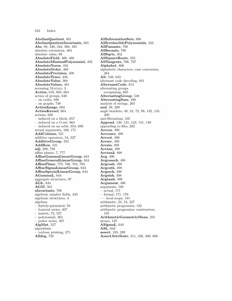
842 Index
AbelianQuotient, 601AbelianQuotientInvariants, 601Abs, 88, 340, 342, 368, 495absolute extensions, 464absolute value, 88AbsoluteField, 466, 468AbsoluteMinimalPolynomial, 456AbsoluteNorm, 456AbsoluteOrder, 468AbsolutePrecision, 408AbsoluteTrace, 456AbsoluteValue, 368AbsoluteValues, 481accessing Magma, 3Action, 610, 663, 664action of groups, 648– on codes, 820– on graphs, 748ActionImage, 664ActionKernel, 664actions, 638– induced on a block, 657– induced on a G-set, 664– induced on an orbit, 654, 690actual arguments, 168, 171AddColumn, 521additive operators, 54, 327AdditiveGroup, 352AddRow, 521adj, 299, 738affine planes, 7, 777AffineGammaLinearGroup, 644AffineGeneralLinearGroup, 644AffinePlane, 778, 780, 783, 794AffineSigmaLinearGroup, 644AffineSpecialLinearGroup, 644AGammaL, 644aggregate structures, 97AGL, 644AGM, 501aInvariants, 706algebraic number fields, 443algebraic structures, 4algebras– finitely-presented, 58– Laurent series, 407– matrix, 72, 527– polynomial, 364– power series, 407AlgMat, 527algorithms– verbose printing, 271Alldeg, 738
AllInformationSets, 806AllIrreduciblePolynomials, 432AllPassants, 796AllSecants, 796AllSqrts, 352AllSquareRoots, 352AllTangents, 796, 797Alphabet, 806alphabetic characters, case conversion,
264Alt, 548, 643alternant code decoding, 831AlternantCode, 812alternating groups– recognizing, 665AlternatingGroup, 548AlternatingSum, 499analysis of strings, 263and, 38, 299angle brackets, 48, 52, 72, 98, 132, 135,
409anti-Hermitian, 535Append, 120, 121, 123, 131, 140appending to files, 282Arccos, 498Arccosec, 498Arccot, 498Arcsec, 498Arcsin, 498Arctan, 498Arctan2, 498Arg, 496Argcosech, 498Argcosh, 498Argcoth, 498Argsech, 498Argsinh, 498Argtanh, 498Argument, 496arguments, 168– actual, 171– formal, 171, 176– – local scope, 181arithmetic, 24, 54, 327arithmetic progression, 122arithmetic progression constructors,
105ArithmeticGeometricMean, 501arrays, 125ASigmaL, 644ASL, 644assert, 195, 299AssertAttribute, 411, 436, 490, 686
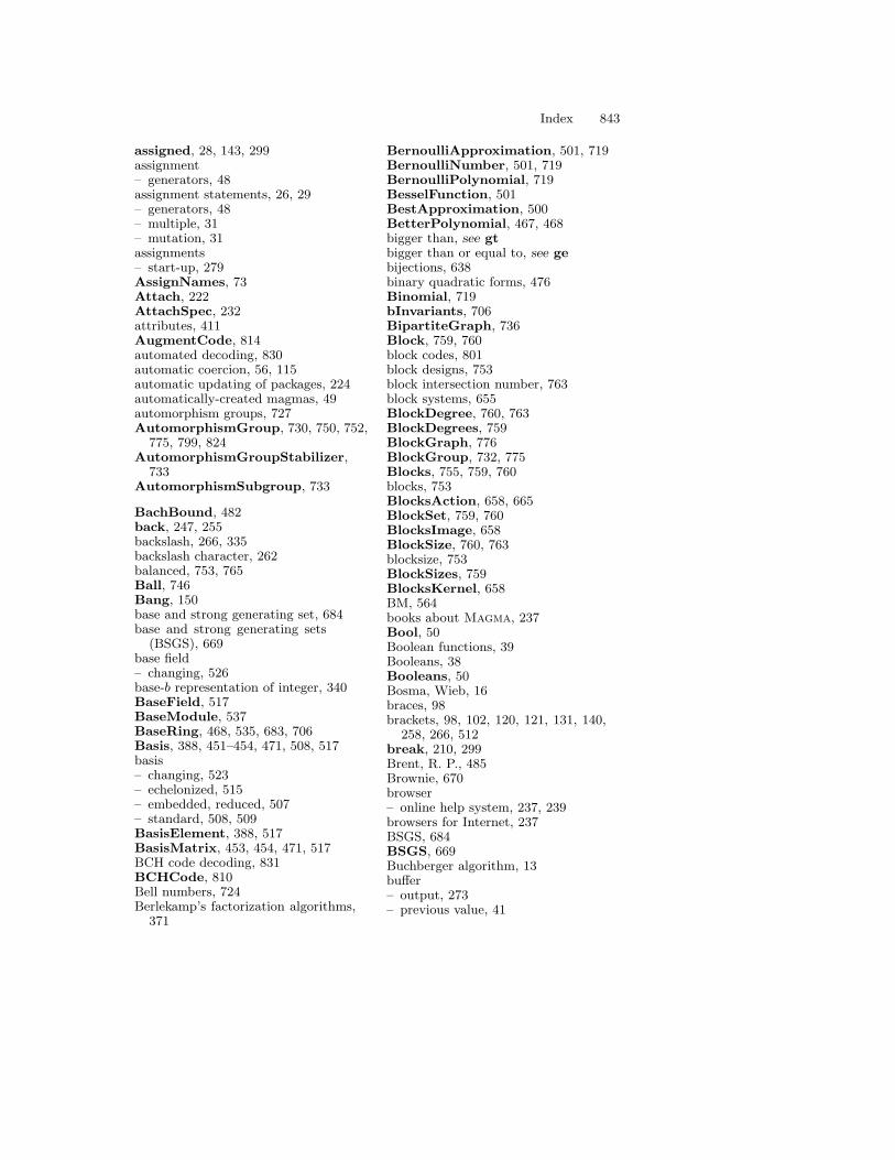
Index 843
assigned, 28, 143, 299assignment– generators, 48assignment statements, 26, 29– generators, 48– multiple, 31– mutation, 31assignments– start-up, 279AssignNames, 73Attach, 222AttachSpec, 232attributes, 411AugmentCode, 814automated decoding, 830automatic coercion, 56, 115automatic updating of packages, 224automatically-created magmas, 49automorphism groups, 727AutomorphismGroup, 730, 750, 752,
775, 799, 824AutomorphismGroupStabilizer,
733AutomorphismSubgroup, 733
BachBound, 482back, 247, 255backslash, 266, 335backslash character, 262balanced, 753, 765Ball, 746Bang, 150base and strong generating set, 684base and strong generating sets
(BSGS), 669base field– changing, 526base-b representation of integer, 340BaseField, 517BaseModule, 537BaseRing, 468, 535, 683, 706Basis, 388, 451–454, 471, 508, 517basis– changing, 523– echelonized, 515– embedded, reduced, 507– standard, 508, 509BasisElement, 388, 517BasisMatrix, 453, 454, 471, 517BCH code decoding, 831BCHCode, 810Bell numbers, 724Berlekamp’s factorization algorithms,
371
BernoulliApproximation, 501, 719BernoulliNumber, 501, 719BernoulliPolynomial, 719BesselFunction, 501BestApproximation, 500BetterPolynomial, 467, 468bigger than, see gtbigger than or equal to, see gebijections, 638binary quadratic forms, 476Binomial, 719bInvariants, 706BipartiteGraph, 736Block, 759, 760block codes, 801block designs, 753block intersection number, 763block systems, 655BlockDegree, 760, 763BlockDegrees, 759BlockGraph, 776BlockGroup, 732, 775Blocks, 755, 759, 760blocks, 753BlocksAction, 658, 665BlockSet, 759, 760BlocksImage, 658BlockSize, 760, 763blocksize, 753BlockSizes, 759BlocksKernel, 658BM, 564books about Magma, 237Bool, 50Boolean functions, 39Booleans, 38Booleans, 50Bosma, Wieb, 16braces, 98brackets, 98, 102, 120, 121, 131, 140,
258, 266, 512break, 210, 299Brent, R. P., 485Brownie, 670browser– online help system, 237, 239browsers for Internet, 237BSGS, 684BSGS, 669Buchberger algorithm, 13buffer– output, 273– previous value, 41

844 Index
bugs, 195built-in functions and procedures, 167by, 105, 299
cached data, 85call-by-name evaluation, 92, 94call-by-value evaluation, 38calling (invoking) functions/procedures,
168calls, see invocationsCannon, 670canonical forms of elements, 57CanonicalGraph, 752Cantor-Zassenhaus factorization
algorithm, 371capital letters, 264car, 98, 132cardinality, 83, 114, 132, 135, 331, 420– finite, infinite, 133Carlson, Jon, 9CarmichaelLambda, 343, 359carrier sets, 727Cartesian product, 132cartesian products, 98CartesianPower, 132CartesianProduct, 132, 744case, 92, 94, 299case of alphabetic characters, 264cat, 120–122, 131, 140, 255, 258, 299Catalan, 497Catalan numbers, 417categories, 46Category, 46, 325, 327cd, 241, 255Ceiling, 342, 495CentralCollineationGroup, 799Centre, 330ChangeDirectory, 277ChangeRing, 526ChangeUniverse, 104changing the basis of a vector space,
523changing the coefficient field of a vector
space, 526Characteristic, 330, 420CharacteristicPolynomial, 432, 440,
539characters, 257, see stringsCharacterTable, 462Check, 758, 780checking for bugs, 195CheckPolynomial, 811ChienChoyCode, 812
ChineseRemainderTheorem, 349cInvariants, 706Class, 567Classes, 14, 567ClassGroup, 474ClassGroupStructure, 474classical groups, 680classical planes, 777, 782ClassNumber, 474ClassRepresentative, 569clear, 299ClearPrevious, 42Clique, 747CliqueNumber, 747cmpeq, 83, 85, 299CO1, CO2, CO3, 564codes, 727, 801– equivalent, isomorphic, 823CodeToString, 264Codomain, 156, 518Coefficient, 366, 381, 408coefficient field– changing, 526CoefficientField, 510, 517CoefficientRing, 364, 392, 408, 468,
510, 535, 683, 706Coefficients, 366, 380, 381, 408, 706Coercion, 150coercion, 53, 65, 109, 115, 490, 496Cokernel, 520collineation groups, 7CollineationGroup, 799CollineationGroupStabilizer, 799CollineationSubgroup, 799ColonIdeal, 391colourings of graphs, 747combinatorial and incidence structures,
727combinatorics, 417, 719comma, 23commands, 299comments, 40common overstructures, 56commutator, 551commutators, 549comp, 319, 321comparable, 84comparing magma elements, 57comparing ring elements, 328compatible, 115, 118Complement, 517, 743, 766ComplementaryErrorFunction, 501complete, 765, 795

Index 845
complete coset spaces, 609complete sequences, 113CompleteGraph, 736CompleteKArc, 796CompleteUnion, 744CompleteWeightEnumerator, 820Completion, 321completion, 250, 256completion, tab, 289complex fields, 485complex numbers, 35ComplexConjugate, 456, 458, 496ComplexField, 36, 318, 485, 494ComplexToPolar, 37, 496Component, 746Components, 746Composition, 415, 478composition of mappings, 163CompositionFactors, 564concatenate, 120, 121, 258concatenation, 122concrete groups– presentations, 600conditional evaluation, 38conditional expressions, 87, 92conditional statements, 87conditions, turning off checking, 758,
780Conductor, 448, 450, 452congruences, 349Conic, 797conjugacy, 653conjugacy classes, 14ConjugacyClasses, 567Conjugate, 457, 458, 481Conjugates, 481, 567conjugates, 549conjugation, 550ConnectionNumber, 760constants, 497constants in packages, 233constituents, 136constructors, 48– AbelianGroup, 630– Group, 598– MatrixAlgebra, 530– MatrixGroup, 678– elt, 52, 409, 493– func, 171– hom, 157– ideal, 61– lideal, rideal, 61– map, 157
– ncl, 61– proc, 176– quo, 75, 515, 597, 629– random, 126– recformat, rec, 141– rep, 126– sub, 61, 515, 629– arithmetic progression, 105– formal sets, 129– set, sequence, 107, 331– tuple, 134ContainsQuadrangle, 789Content, 368contiguous substring, 259continue, 210, 299ContinuedFraction, 500Contpp, 368Contract, 743Contraction, 766control characters, 291control-c, 293control-d, 255control-n, 292control-p, 292Convergents, 500Convolution, 415ConwayPolynomial, 434Coordinates, 388, 790, 805, 830Cop, 98cop, 98coproducts, 98, 136, 140Core, 611Cos, 415, 498Cosec, 498Cosech, 498coset representatives, 611coset tables, 607, 609CosetAction, 614CosetDistanceDistribution, 819CosetImage, 614CosetKernel, 614cosets– finitely-presented groups, 613CosetSpace, 610, 614Cosh, 415, 498Cot, 498Coth, 498counting theory, 417Covalence, 759, 763CoveringRadius, 819Coxeter, 670CPU time, 33Cputime, 294

846 Index
creating objects, 4creation, 325cube, group of symmetries of, 646curly brackets, see bracescurrent directory, 277current input line, 290CurveEll, 703CurveEllPt, 703customizing Magma, 233cycle form for permutations, 639CycleStructure, 641CyclicCode, 810CyclicGroup, 548CyclotomicField, 447, 448CyclotomicOrder, 448
Darstellungsgruppe, 599data files, 281databases, 835databases of definitions, 42, 277DawsonIntegral, 501Decode, 830decoding, 827Decomposition, 473DedekindEta, 501Default, 269, 270, 281default, 299default precision, 411default real field, 486DefiningPolynomial, 425, 432, 444,
446, 448, 450definitions in libraries and databases,
277Degree, 366, 381, 408, 420, 444,
446–448, 450, 470, 517, 535, 641, 648,663, 683, 738
degree, 443, 638degree of transitivity, 649DegreeOnePrimeIdeals, 473degrees (angles), 498DegreeSequence, 738delete, 28, 143, 285, 299delve, 245, 255Denominator, 37, 342, 366, 385, 470derivation, 7Derivative, 367, 415derived G-sets, 638, 648, 660derived subgroups, 610Desarguesian, 792Design, 766, 800designs, 727, 753, 765Detach, 222DetachSpec, 232
Determinant, 536Development, 769DiagonalJoin, 514DiagonalMatrix, 528Diameter, 746, 819DiameterPath, 746diff, 118, 130, 299difference– of elements, 54, 327– of sets, 118, 130difference sets, 769DifferenceSet, 769digraphs, 735DihedralGroup, 548Dilog, 498Dimension, 392, 517, 535, 806directed graphs, 735directories of files, 277DirectProduct, 599, 645, 682, 814DirectSum, 534, 536, 634, 814Discriminant, 372, 444, 446, 448, 450,
478, 706disjoint cycle form for permutations,
639Distance, 478, 746, 805distance, 818DistinctDegreeFactorization, 371div, 24, 54, 299, 332, 339, 367division, 54, 327, 332– exact, 24– in rings (quotient-and-remainder), 24– integers, 24– quotient, remainder, see QuotremDivisorSigma, 343, 359do, 199, 205, 299documentation of Magma, 237Domain, 156, 518double cosets, 611double quotation mark character, 26,
257, 262Dual, 766, 794, 806DualWeightDistribution, 819dummy variables, 107
e, 486e, 36EARNS, 666EchelonForm, 519, 538echelonized basis, 515echoing external input, 280EdgeGroup, 732, 750, 751Edges, 737edges

Index 847
– addition, subtraction, 739EdgeSet, 737EdgeUnion, 744editing input, 290EDITOR, 293ei, 501Eigenspace, 539Eigenvalues, 539element-description, 107elements, 4, 51– canonical forms, 57– literal, 52– representation, 58– testing membership, 83, 115, 130ElementToSequence, 435, 529, 628,
673elif, 90, 299Eliminate, 594elliptic curves, 703else, 87, 92, 299elt, 52, 134, 135, 336, 409, 493Eltseq, 435, 444, 446, 448, 452, 453,
511, 529, 593, 594, 628, 673, 790Emacs editor, 290Embed, 430, 432embedded basis, 507embedding in complex field, 458embedding of finite fields, 429empty sets and sequences, 104empty word, 593EmptyGraph, 736encoding, 827end, 299endo-trivial modules, 9EndomorphismAlgebra, 524EndVertices, 738entering Magma, 3enumerated sequences, 98enumerated sets, 98enumerative combinatorics, 719environment variables, 278, 279, 296environment, user, 289eq, 57, 83, 115, 132, 135, 299, 327, 391,
593, 729equal to, see eqequality– words in fp-magmas, 56equation orders, 449EquationOrder, 450equivalent codes, 822, 823Erf, 501Erfc, 501error, 299
error-correcting codes, see codesErrorFunction, 501errors, 195, 225errors in sending codewords, 829escape to shell, 286η, 501Euclidean decoding, 831Euclidean decoding algorithm, 831EuclideanNorm, 332EulerGamma, 497EulerianNumber, 719EulerPhi, 343, 359, 447Evaluate, 367, 414evaluation– call-by-name, call-by-value, 92, 94evaluations, 23examples, 7– in the textbooks, 44– online help nodes, 248Exclude, 116, 120, 121ExcludedConjugates, 610exclusive-or, 38execute, 3existential quantifiers, 127exists, 127, 299ExistsConwayPolynomial, 434exit, 255, 299exiting an iteration or loop quickly, 210exiting Magma, 5, 293Exp, 415, 498Explode, 91, 120, 121, 135exponentation, 35exponential numbers, 724ExponentialIntegral, 501exponentiation, 24, 54, 327, 349– modular, 348ExponentSum, 594expressions, 23– case, 94– conditional, 87, 92– regular (strings), 265ExpurgateCode, 814ext, 319, 465ExtendBasis, 525, 526ExtendCode, 814extended greatest common divisor, 339ExtendField, 526ExtensionField, 425extensions– of finitely-presented groups, 599– relative, 455– relative, absolute, 464extensions of finite fields, 423

848 Index
Exterior, 797ExteriorSquare, 534, 536external files and processes, 277external line, 795external processes, 285ExternalLines, 796ExtractGenerators, 622ExtractGroup, 622ExtractRep, 119
Facint, 347FactorBasis, 482FactoredOrder, 435, 536Factorial, 719Factorization, 136, 332, 356, 369, 473factorization, 16factorization sequences, 136, 345FactorizationToInteger, 347false, 38, 50, 299families of groups, 564Fibonacci, 112, 719Field, 806field of fractions, 322FieldOfFractions, 322, 365, 385, 449,
450fields, 317– complex, 485– cyclotomic, 447– finite (Galois), 51, 351, 419– number, 16, 443– quadratic, 446– rational, 335, 443– real, 485– residue, 323File, 282file objects, 282files, 277– data, 281– input, 42, 277– log, output, 281– start-up, 278find, 243, 255finite fields, 51finite geometry, 7, 777finite planes, 7, 777FiniteField, 318, 351, 419finitely-presented, 78finitely-presented abelian groups, 629finitely-presented groups, 591, 595– cosets, permutation representations,
613– quotients, 601– subgroups of finite index, 619
finitely-presented magmas, 58, 59finitely-presented subgroups– subgroup presentation, 615First Steps in Magma, Vfirst textual use rule, 181first-class objects, 170, 183Fix, 641, 648, 664, 823fixed precision real/complex fields, 485fixed precision series rings, 408fixed-point set, 648flags, verbose printing, 271Flat, 132FldCyc, 444FldNum, 444FldPr, 50FldQuad, 444FldRat, 50, 443Floor, 342, 495flushing the output buffer, 273for, 205, 299, 331forall, 127, 299formal arguments, 168, 171, 176– local scope, 181formal sets, 98, 129FormalSet, 83, 129, 648Format, 143format string, 272formats for records, 141formatted printing, 272forms– binary quadratic, 476forward, 185, 299fp, see finitely-presentedFPGroup, 600free identifiers, 107free magmas, 50, 78free precision series rings, 408free real/complex fields, 485free reductions, 58, 594FreeAbelianGroup, 544, 627FreeGroup, 50, 544, 592FreeProduct, 599freeze, 224, 299frozen packages, 224full matrix space, 508full pathnames, 277full vector space, 507func, 171Function, 159function, 299function assignment statements, 187function expressions– constructor form, 171

Index 849
– statement form, 174, 187function fields, 323, 365, 385FunctionField, 318, 323, 365functions, 167– return, 174– Boolean, 39– defined recursively, 183, 188– intrinsic, 25– principal value, 32– returning several values, 31, 172– signatures, 216– transfer, 146– user-defined, 170fundamental units, 479FundamentalUnit, 476
G-invariant, 638, 654, 655G-set, 730G-sets, 638– derived, 660– general, 660– natural, 639– standard, 638Galois correspondences, 16Galois groups, 457GaloisField, 51, 419GaloisGroup, 17Γ , 497, 501Gamma, 501γ, 501GammaD, 501GCD, 196, 332, 339, 347, 367Gcd, 339ge, 57, 299, 331, 593general element in aggregate
constructor, 107general G-sets, 660general incidence structures, 727‘general’ number fields, 443GeneralizedSrivastavaCode, 812GeneralLinearGroup, 546, 672, 680GeneralUnitaryGroup, 681generating functions, 417, 726GeneratingWords, 601Generator, 350, 352, 421, 422generator assignments, 48GeneratorMatrix, 806GeneratorNumber, 594GeneratorPolynomial, 811Generators, 66, 471, 508, 517, 601,
648, 712generators, 58, 515– naming, 72
Generic, 63, 391, 517, 531, 535, 648,679, 683
generic magmas, 63Geodesic, 746geometry– finite, 7, 777GetAssertions, 196Getc, 282GetCurrentDirectory, 277GetDefaultRealField, 487, 491GetEchoInput, 280GetHistorySize, 291GetMemoryLimit, 296GetPath, 278Getpid, 287GetPreviousSize, 41Gets, 282GetVerbose, 271GF, 419Girth, 746GirthCycle, 746GL, 81, 546, 672, 680GolayCode, 809Goppa code decoding, 831GoppaCode, 812goto, 241, 255grammar, 303graphs, 727, 735– group action, 748– standard, 736– standard constructions, 743– tests, 745– unions and products, 744greater than, see gtgreater than or equal to, see gegreatest common divisor, 339, see
GCDGreatestCommonDivisor, 339Groebner, 388GroebnerBasis, 388GroundField, 424, 464, 468Group, 544, 598, 663group actions, 638groups, 543– abelian, 79, 627– abelian (not in GrpAb), 633– action, 648– action on codes, 820– action on graphs, 748– categories, 547– class, 473– classical, 680– commutator, 551
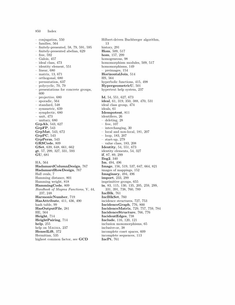
850 Index
– conjugation, 550– families, 564– finitely-presented, 58, 79, 591, 595– finitely-presented abelian, 629– free, 592– Galois, 457– ideal class, 473– identity element, 551– linear, 680– matrix, 13, 671– orthogonal, 680– permutation, 637– polycyclic, 70, 79– presentations for concrete groups,
600– projective, 680– sporadic, 564– standard, 548– symmetric, 639– symplectic, 680– unit, 473– unitary, 680GrpAb, 543, 627GrpFP, 543GrpMat, 543, 672GrpPC, 543GrpPerm, 543GRSCode, 809GSet, 639, 648, 661, 662gt, 57, 299, 327, 331, 593GU, 681
HA, 564HadamardColumnDesign, 767HadamardRowDesign, 767Hall ovals, 7Hamming distance, 801Hamming weight, 818HammingCode, 809Handbook of Magma Functions, V, 44,
237, 248HarmonicNumber, 719HasAttribute, 411, 436, 490hash table, 99HasOutputFile, 281HE, 564Height, 714HeightPairing, 714help, 255help on Magma, 237HenselLift, 372Hermitian, 535highest common factor, see GCD
Hilbert-driven Buchberger algorithm,13
history, 291Hom, 509, 517hom, 157, 299homogeneous, 98homomorphism modules, 509, 517homomorphisms, 149– preimages, 154HorizontalJoin, 514HS, 564hyperbolic functions, 415, 498HypergeometricU, 501hypertext help system, 237
Id, 54, 551, 627, 673ideal, 61, 319, 350, 388, 470, 531ideal class group, 474ideals, 61Idempotent, 811identifiers, 26– deleting, 28– free, 107– interchanging, 30– local and non-local, 181, 207– loop, 183, 207– start-up, 279– value class, 183, 208Identity, 54, 551, 673identity elements, 54, 327if, 87, 89, 299Ilog2, 340Im, 494, 496Image, 156, 519, 537, 647, 664, 821images of mappings, 152Imaginary, 494, 496import, 233, 299imprimitive groups, 655in, 83, 115, 130, 135, 205, 259, 299,
331, 391, 738, 760, 789IncBlk, 761IncBlkSet, 760incidence structures, 727, 753IncidenceGraph, 776, 800IncidenceMatrix, 729, 757, 759, 784IncidenceStructure, 766, 776IncidentEdges, 738Include, 116, 120, 121inclusion monomorphisms, 65inclusive-or, 38incomplete coset spaces, 609incomplete sequences, 113IncPt, 761

Index 851
IncPtSet, 760IndependenceNumber, 747Independent, 747IndependentUnits, 479Index, 114, 258, 470, 607indexed sets, 98IndexedSetToSequence, 146IndexedSetToSet, 146indexing vectors and matrices, 512induced actions, 654, 657, 664, 690infinite series, 499, 725infinite sets, 129, 130InfiniteSum, 499InformationSet, 806InformationSpace, 806InnerProduct, 512, 805input, 3, 274– echoed from files, 280– long input lines, 262input files, 42, 277input, editing, 290Insert, 120, 121, 124InsertBlock, 514InsertVertex, 743integer arithmetic, 24, 36integer part of nth root, 340integer part of square root, 340integer-string, 263IntegerRing, 50, 318, 322, 336, 365,
385, 450Integers, 336integers, 35integers in base-b representation, 340IntegerToString, 263Integral, 195, 415IntegralBasis, 450, 451IntegralModel, 709, 710interacting with Magma, 3interface, user, 237Interior, 797Internet browsers, 237interrupting a computation, 293intersection, 83, 118, 130, 330IntersectionArray, 750IntersectionNumber, 763intrinsic, 299intrinsics, 25, 167, 215– help nodes, 248– signatures, 216An Introduction to Magma, V, 44Intseq, 340InvariantFactors, 539InvariantRing, 697
Invariants, 631, 634invariants, 13InvariantsOfDegree, 15, 697inverse elements, 54, 327inverse trigonometric and hyperbolic
functions, 415, 498invocations of functions/procedures,
168, 176Iroot, 340IrreduciblePolynomial, 425, 432is, 33, 299IsAbelian, 559IsAlternating, 665IsAltSym, 665IsArc, 796IsAssociate, 332IsBalanced, 765IsBipartite, 39, 745IsBlock, 657, 760IsBlockTransitive, 775IsCentral, 559IsCentralCollineation, 799IsCollinear, 789IsCommutative, 329IsComplete, 113, 610, 745, 765, 796IsConcurrent, 789IsConjugate, 559, 612, 653, 664IsConnected, 746IsConsistent, 523IsConway, 434IsCyclic, 559, 807IsDefined, 113IsDesarguesian, 792IsDesign, 765IsDiagonal, 536IsDifferenceSet, 769IsDistanceRegular, 750IsDistanceTransitive, 750IsDivisible, 332, 339IsDivisionRing, 329IsDomain, 329IsEdgeTransitive, 750, 751IsElementaryAbelian, 559IsEllipticCurve, 705IsEmpty, 104, 131, 140, 624, 745IsEof, 282IsEquationOrder, 450IsEquivalent, 823Isetseq, 146Isetset, 146IsEuclideanDomain, 329, 332IsEuclideanRing, 329, 332IsEulerian, 746

852 Index
IsEven, 339, 347, 641IsExtraSpecial, 559IsFaithful, 664IsField, 329IsFinite, 329, 330IsForest, 745IsFrobenius, 650IsHadamard, 767IsHadamardEquivalent, 767IsId, 54, 57, 627IsIdempotent, 328IsIdentity, 54, 57IsIndependent, 525IsInRadical, 391IsIntegral, 336, 342, 450, 455, 473, 496IsIntegralDomain, 329IsInvariant, 697IsIrreducible, 328, 371, 383, 432IsIsomorphic, 468, 710, 729, 752, 817,
823IsLinearGroup, 695IsLinearSpace, 765IsLineRegular, 765IsLineTransitive, 799IsMaximal, 401, 450, 559, 612IsMDS, 807IsMinusOne, 328, 478, 496IsNearLinearSpace, 765IsNilpotent, 328, 559IsNormal, 438, 559, 612IsNull, 104IsOdd, 339, 347, 641isomorphic, 729isomorphic codes, 822, 823isomorphisms, 467, 727IsOne, 54, 57, 328, 347, 478, 496IsOrbit, 652IsOrdered, 329IsOrthogonalGroup, 695IsOrthogonalType, 695IsParallel, 789IsParallelClass, 760IsPath, 745IsPerfect, 559IsPID, 329IsPIR, 329IsPointRegular, 765IsPointTransitive, 775, 799IsPolygon, 745IsPower, 457IsPowerTimesUnit, 457IsPrimary, 401IsPrime, 328, 347, 354, 473
IsPrimePower, 347IsPrimitive, 349, 352, 422, 432, 457,
657, 664, 750IsPrincipal, 473IsPrincipalIdealDomain, 329IsPrincipalIdealRing, 329IsProper, 391Isqrt, 340IsRadical, 401IsReal, 496IsReduced, 478IsRegular, 328, 650, 664, 738IsRelative, 454IsResolvable, 765IsScalar, 536IsSelfDual, 765, 792, 807IsSelfNormalizing, 559IsSelfOrthogonal, 807IsSemiregular, 650, 664IsSemisimple, 532IsSharplyTransitive, 650, 664IsSimilar, 536IsSimple, 532, 559, 765IsSoluble, 559IsSolvable, 559IsSpecial, 559IsSpecialLinearGroup, 695IsSpecialOrthogonalGroup, 695IsSpecialUnitaryGroup, 695IsSquare, 352, 435IsSquareFree, 347IsSteiner, 765IsSubnormal, 559IsSubsequence, 122IsSymmetric, 536, 665, 750, 765IsSymplecticGroup, 695IsSymplecticType, 695IsTransitive, 650, 664, 750, 799IsTree, 745IsTrivial, 765IsUFD, 329IsUniform, 765IsUniqueFactorizationDomain, 329IsUnit, 328, 347, 455, 529IsUnital, 797IsUnitary, 329IsUnitaryGroup, 695IsUnitaryType, 695IsVertexTransitive, 750IsWeaklySelfDual, 807IsWeaklySelfOrthogonal, 807IsZero, 54, 57, 328, 391, 473, 496, 511IsZeroDivisor, 328

Index 853
iterable, 98iterable homogeneous aggregates, 100,
114iterable magmas, 107, 206iteration, 133, 331iterative statements, 197– nested, 212– quick exit, 210
J1, J2, J3, J4, 564JacobiSymbol, 343, 359JacobiTheta, 501JacobiThetaNull, 501JacobsonRadical, 532JBessel, 501jInvariant, 501, 706join, 118, 130, 299, 761JordanForm, 539
K-modules, 507k-ply transitive, 649kArc, 796KBessel, 501KBessel2, 501KCubeGraph, 736Kernel, 156, 520, 537kinds of help nodes, 248KMatrixSpace, 55, 508Knot, 797KSpace, 507
Labelling, 663labelling information, 26λ, 343, 359language, 303Laplace, 415large-prime polynomial factorization,
371LargestClique, 747LargestIndependent, 747Laurent series rings, 321LaurentSeriesAlgebra, 408LaurentSeriesRing, 318, 408, 412LCM, 332, 339, 347, 367Lcm, 339le, 57, 299, 331, 593LeadingCoefficient, 366, 380, 381LeadingMonomial, 366, 380LeadingTerm, 366, 380, 381least common multiple, see LCMleaving Magma, 5, 293left ideal, 531left-normed commutators, 549LegendreSymbol, 343, 359
Length, 481, 806length– of a sequence, 115– of a string, 258– of a word, 593LengthenCode, 814Leon, 670less than, see ltless than or equal to, see lelevels of printing, 269, 270, 281lexicographic ordering– strings, 260– words in free group, 594LexProduct, 744Li, 498li, 501libraries of definitions, 42, 277lideal, 61, 531Lift, 708limits on memory, 295Line, 760line continuation, 262line continuation character, 335line editor, 290line regular, 765linear algebra, 537linear codes, 801– encoding and decoding, 827– group action, 820– noisy communications channel, 804– operations, 814– weight distribution, 818linear congruences, 349linear groups, 680linear spaces, 727, 753, 765linear transformations, 509, 517LinearCode, 81, 776, 800, 802, 803LinearSpace, 766LineGraph, 743, 800LineGroup, 732, 799LineOrbits, 689Lines, 784, 785lines, 753lines of input, editing, 290LineSet, 784, 785List, 98, 130ListCategories, 47lists, 98, 130, 131ListSignatures, 218literal, 23literal elements, 52load, 42, 299loc, 319, 322

854 Index
local, 299local identifiers, 181, 207local scope, 107LocalHeight, 714locality, principle of, 64Localization, 322Log, 415, 434, 435, 498log file, 281LogDerivative, 501LogGamma, 501LogIntegral, 501Logs, 481long input lines, 262loop identifiers, 183, 207loops, 197– nested, 212– quick exit, 210lower case letters, 264lowest common multiple, 339, see LCMLowestCommonMultiple, 339LowIndexProcess, 622LowIndexSubgroups, 619ls, 240, 255lt, 57, 299, 331, 496, 593LY, 564
M(22), M(23), M(24), 564M, M11, M12, M22, M23, M24, 564MacWilliamsTransform, 819, 820MagForm, 477MagFormElt, 477Magma print-level, 269, 270, 281Magma, V, 3– documentation, 237– entering, 3– interrupting, 293– multiple processes, 287– online help, 237– quitting, 5, 293– user environment, 289Magma HTML Help Document, 237MAGMA_MEMORY_LIMIT, 296MAGMA_PATH, 277, 278MAGMA_STARTUP_FILE, 279MAGMA_USER_SPEC, 232magmas, 4, 45– automatically-created, 49– finitely-presented, 78– free, 50, 78– generators of, 66– generic, 63– ideals, 61– iterable, 107, 206
– normal closures, 61– operations, 83– quotients, 75– submagmas, 61– warning about, 85MantissaExponent, 487manuals on Magma, 237map, 157mapping form for permutations, 639mappings, 149, 170– defined recursively, 163– images, 152– preimages, 154mark, 252, 255marks, 252, 255Match, 594matrices– constructing, 511matrix algebras, 527matrix groups, 13, 543, 671– natural R-module, 687matrix modules, 537matrix rings, 527matrix spaces, 55, 507, 530, 537, 674MatrixAlgebra, 81, 392, 439, 440,
527, 530MatrixGroup, 81, 678MatrixRing, 72, 81, 527MatrixUnit, 528Max, 331, 340Max, see MaximumMaxdeg, 738Maximal, 269, 270, 281maximal orders, 449MaximalIdeals, 532MaximalLeftIdeals, 532MaximalOrder, 450MaximalOvergroup, 611MaximalPartition, 657MaximalRightIdeals, 532Maximum, 116, 331maximum-distance separable codes, 807MaxNorm, 368MCL, 564meet, 83, 118, 130, 299, 330, 391, 517,
761, 789memory limits, 295MergeFields, 467, 468MergeUnits, 479Miller-Rabin probabilistic primality
test, 354Min, 331, 340Min, see Minimum

Index 855
Mindeg, 738Minimal, 269, 270, 281MinimalField, 460MinimalIdeals, 532MinimalInteger, 470MinimalLeftIdeals, 532MinimalModel, 710MinimalNormalSubgroups, 667MinimalOvergroup, 611MinimalPartition, 657MinimalPartitions, 657MinimalPolynomial, 432, 440, 455,
461, 539MinimalRightIdeals, 532Minimize, 460Minimum, 116, 184, 331MinimumDistance, 806, 819MinimumWeight, 806, 819MinimumWords, 819MinkowskiBound, 482miscellaneous features, 289mod, 24, 54, 299, 332, 339, 367Modexp, 348, 349Modinv, 349ModMatFld, 507ModMatRng, 507, 510Modsqrt, 349ModTupFld, 507ModTupRng, 507, 510modular exponentiation, 348modules, 9, 507, 537– matrix, 537Modulus, 351, 352, 496MoebiusMu, 343, 347, 359Molien series, 13MolienSeries, 697monoids, 79monoids, finitely-presented, 58monomial actions on a code, 820MonomialCoefficient, 366, 380MonomialGroup, 824Monomials, 366, 380MonomialsOfDegree, 697monomorphisms, 65MonStg, 50, 258MonStgElt, 258MordellWeilGroup, 712MordellWeilRank, 712MordellWeilRankBounds, 712more, 255Morphism, 516, 534MP, 485µ, 343, 359
multi-dimensional sequences, 125multi-index, 120, 125, 131multi-sorted algebras, 727multi-valued expressions, 31Multinomial, 719MultipartiteGraph, 736multiple assignment statements, 31multiple extensions, 464multiple Magma processes, 287multiplication of permutations, 640MultiplicationTable, 454multiplicative operators, 54, 327MultiplicativeGroup, 352, 353MultiplicatorRing, 473Multiplicity, 101MultiplyColumn, 521MultiplyRow, 521Multisets, 721multisets, 98MultisetToSet, 146mutation, 120mutation assignment, 31mutual recursion, 186
NaiveHeight, 714Names, 143natural G-sets, 639natural G-sets and actions, 638ncl, 61Ncolumns, 536ne, 57, 83, 115, 299, 327, 593, 729near-linear spaces, 727, 753, 765NearLinearSpace, 766negative, 54Neighbours, 738nested sequences, 125nested statements, 212newline character, 262newlines, 265NextPrime, 360NextSubgroup, 623Ngens, 66, 517, 601, 648Nickel, Werner, 605Niemeyer, Alice, 605nilpotent quotients, 605nodes, online help, 239noisy communications channel, 804non-local identifiers, 181Norm, 435, 455, 470, 495, 496normal closures, 61NormalClosure, 611NormalElement, 438NormalForm, 391

856 Index
Normalize, 512Normalizer, 611NormEquation, 349, 455, 456not, 38, 299not equal to, see nenotadj, 299, 738notin, 83, 115, 130, 259, 299, 738, 760,
789notsubset, 83, 115, 299, 760, 789Nrows, 536null sets and sequences, 104NullSpace, 520, 538number fields, 16, 443number of elements, see cardinalitynumber theory, 335– factorization, 353, 356– primality, 353NumberField, 318, 444, 445NumberOfBlocks, 759NumberOfColumns, 536NumberOfComponents, 132NumberOfDivisors, 347NumberOfGenerators, 66NumberOfLines, 784NumberOfPartitions, 722NumberOfPermutations, 719NumberOfPoints, 759, 784NumberOfRows, 536NumberOfWords, 819numbers, 35– complex, 485, 494– integers, 24, 335– rationals, 335– real, 485numbers, 252, 255Numerator, 37, 342, 366, 385
O’Nan, 665objects, 4ON, 564on-the-fly invocations, 170One, 54, 325, 327, 496online examples, see examplesonline help, 237Open, 282operating system access, 285operators, 217– arithmetic, 24– Boolean, 38– order of evaluation, 25– precedence, 301– relational, 38, 115, 258or, 38, 299
Orbit, 652, 664, 688OrbitAction, 654, 665, 690OrbitActionBounded, 690OrbitImage, 654, 690OrbitImageBounded, 690OrbitKernel, 654, 690OrbitKernelBounded, 690Orbits, 652, 664, 689OrbitsPartition, 750Order, 83, 349, 352, 435, 440, 536, 551,
624, 712, 738, 763, 792order of operations, 25ordering, 102– strings, 260– words in free group, 593orders, 444, 449orthogonal groups, 680output, 3, 23, 25– scrolling, 294– stored as strings, 270output file, 281ovals, 7OverDimension, 517overview kind of help node, 248overwriting files, 282
p-adic fields, 321p, 489, 492package files, 221package spec files, 231packages, 215pAdicField, 318, 321pAdicRing, 318ParallelClass, 789ParallelClasses, 789Parameters, 763parameters, 191Parent, 46, 102, 135, 325, 327parent node in online help, 242ParentGraph, 738parentheses, 25, 266ParentPlane, 784PARI, 485ParityCheckMatrix, 806parser, 278partial maps, 150partial quotients, 500Partitions, 722partitions, 655PascalTriangle, 763passant, 795PathGraph, 736pathname of help node, 242

Index 857
pathnames– full, relative, 277pattern-matching, 265PCGroup, 544Pencil, 789permutation actions on a code, 820permutation groups, 637– action, 648– imprimitive, primitive, 655– projective, 680– transitive, 649permutation representations, 638permutation representations of
fp-groups, 613PermutationGroup, 81, 642, 824Permutations, 721pFundamentalUnits, 479PGammaL, 644, 680PGammaU, 644PGL, 644, 680PGU, 644φ, 343, 359Pi, 495, 497π, 497Pipe, 286pipe, 286PlaneAff, 777PlaneLn, 785PlaneLnSet, 777, 785PlaneProj, 777PlanePt, 785PlanePtSet, 777, 785planes, 727– classical, 782– finite (affine, projective), 7, 777PlotkinSum, 814pmap, 150Point, 759point regular, 765PointDegree, 760PointDegrees, 759PointGraph, 776, 800PointGroup, 775, 799Points, 755, 759, 760, 784, 785points, 638, 753PointSet, 759, 760, 784, 785PolarToComplex, 495, 496polycyclic groups, 543PolygonGraph, 736Polylog, 498PolylogD, 498PolylogDold, 498PolylogP, 498
polynomial rings, 16, 321PolynomialAlgebra, 364PolynomialRing, 318, 364polynomials– polynomials– – better, 467– Conway, 433– for finite fields, 432POmega, 644POmegaMinus, 644POmegaPlus, 644POpen, 282, 287Position, 114, 120, 258PositiveSum, 499, 725Power, 478power printing, 436power series, 13power, raising to a, 24, 54, 327, 349PowerSeriesAlgebra, 408PowerSeriesRing, 318, 408, 412PowerSet, 721pPrimaryComponent, 633, 634pPrimaryInvariants, 633, 634pQuotient, 603pRadical, 473pRank, 792precedence of operators, 25, 301Precision, 412, 413, 486, 487precision, 407, 411– arbitrary, 36– changing, 493preimages, 76, 154presentation, 78presentation for subgroup of fp-group,
615presentations for concrete groups, 600previous sessions, returning, 285previously printed values, recalling, 40PreviousPrime, 360primality, 353primary invariants, 13PrimaryDecomposition, 401PrimaryInvariantFactors, 539PrimaryInvariants, 633, 634, 697PrimaryRationalForm, 539Prime, 401prime field, 419prime numbers, generating, 360PrimeField, 330, 424PrimeForm, 478PrimeRing, 330primitive, 422primitive elements, 443

858 Index
primitive groups, 655, 665PrimitiveElement, 351, 352, 423,
434, 444PrimitivePart, 368PrimitivePolynomial, 432PrimitiveRoot, 349, 351principal argument of complex number,
496principal value of a function, 32principle of locality, 64print, 23, 269, 299printed values, recalling, 40printf, 272, 299PrintFileMagma, 282printing– formatted, 272printing an object to a file, 281printing an object to a string, 270printing finite field elements, 436printing text, 26printname, 48proc, 176procedure, 299procedure assignment statements, 187procedure expressions– constructor form, 176– statement form, 177, 187procedures, 167– return, 180– defined recursively, 183, 188– signatures, 216– user-defined, 176– variable reference arguments, 116process, 622process space, 28processes– Magma, 287– external, 285products, 24, 54, 327– Cartesian, 132– of finitely-presented groups, 599– of permutation groups, 645progressions, arithmetic, 105projective groups, 680projective planes, 7, 777ProjectiveEmbedding, 794ProjectiveGammaLinearGroup,
644ProjectiveGammaUnitaryGroup,
644ProjectiveGeneralLinearGroup,
644
ProjectiveGeneralUnitaryGroup,644
ProjectiveOmegaGroup, 644ProjectiveOmegaMinusGroup, 644ProjectiveOmegaPlusGroup, 644ProjectivePlane, 778, 780, 782ProjectiveSigmaLinearGroup, 644ProjectiveSigmaSymplecticGroup,
644ProjectiveSigmaUnitaryGroup,
644ProjectiveSpecialLinearGroup, 644ProjectiveSpecialUnitaryGroup,
644ProjectiveSuzukiGroup, 644ProjectiveSymplecticGroup, 644prompt symbols, 3, 88, 199Prune, 120, 121, 124, 131, 140Ψ , 501Psi, 501PSigmaL, 644, 680PSigmaSp, 644PSigmaU, 644PSL, 644, 680PSp, 644PSU, 644PSz, 644PunctureCode, 814Put, 282Puts, 282pwd, 241, 255
QRCode, 810quadratic forms, 476QuadraticField, 446QuadraticForm, 797quantifiers, existential and universal,
127quit– saving workspace, 285quit, 5, 255, 299quo, 75, 319, 323, 351, 515, 597, 629quotient, 54, 327, 332, 339quotient groups, 601quotient magmas, 75quotient, remainder, see Quotremquotients– quotient rings as residue class fields,
323Quotrem, 54, 332, 339, 367
R-(tuple) spaces, 510R-matrix spaces, 507, 510

Index 859
R-modules, 507R-spaces, 507radians, 498Radical, 401RadicalDecomposition, 401radix representation of integers, 340raising to a power, 24, 54, 327, 349RamificationIndex, 470Random, 83, 126, 132, 325, 327, 340,
511, 594, 635, 759, 760, 784, 789random, 126, 299RandomBits, 340RandomGraph, 736RandomProcess, 635RandomSchreier, 670, 685RandomTree, 736Rank, 364, 392, 519, 536, 712RankBounds, 712rational approximations, 500rational arithmetic, 36rational field, 443rational function fields, 323, 365, 385rational functions, 13RationalField, 50, 318, 336RationalForm, 539RationalReconstruction, 341, 342Rationals, 336rationals, 35Re, 494, 496Read, 281read, 274, 299readi, 274, 299reading data files, 281Real, 494, 496real fields, 485real numbers, 35RealField, 50, 318, 485, 491Rec, 98rec, 98, 141recalling previously printed values, 40recformat, 98, 141RecFrmt, 98recognizing alternating and symmetric
groups, 665record formats, 98records, 98, 141rectangular matrices, 530, 674recursion, 112, 163, 183, 188, 725– mutual, 186reduced basis, 507reduced form for rationals, 336ReducedDiscriminant, 444, 450Reduction, 478
reduction, 117, 659ReductionStep, 478Reductum, 366Reed-Solomon code decoding, 831ReedMullerCode, 809ReedSolomonCode, 809reference arguments, 169reference counts, 180reference to help node, 244reflection groups, 13Regexp, 265regexp, 267regular– point, line, 765regular expressions, 265Regulator, 474, 481, 714relation normal subgroup, 595relational operators, 38, 57, 115, 258RelationMatrix, 482Relations, 601relations for group presentation, 597relative extensions, 455, 464relative pathnames, 277RelativePrecision, 408remainder, 54, 332, 339Remove, 120, 121, 124Rep, 83, 119, 126, 132, 325, 327, 759,
760, 784, 789rep, 126repeat, 202, 299repeated elements, aggregates with, 99ReplicationNumber, 763representation of elements, 58RepresentationMatrix, 454representations– permutation, 638representations of fp-groups, 613Representative, 325, 327representative elements, 83, 119, 126require, 299requirege, 299requirerange, 299reserved words, 27, 299Residual, 766ResidueClassField, 323ResidueClassRing, 351resolution, 765resolvable, 765restore, 285, 299RestrictedPartitions, 722RestrictField, 526Restriction, 766Resultant, 372

860 Index
return– functions, 174– procedures, 180return, 299return character, 262return values of functions, 169, 172returning to a previous session, 285Reverse, 120, 121, 124Reversion, 415Rewind, 282Rewrite, 616ReynoldsOperator, 15rideal, 61, 531Riemann zeta function, 501right ideal, 531ring of integers, 322, 365, 385, 449rings, 317– integer, 36, 335– Laurent series, 407– matrix, 72, 527– polynomial, 16, 364– power series, 407RMatrixSpace, 510RngInt, 50RngIntRes, 351RngMPol, 377RngUPol, 364Root, 435, 457, 495root– integer part, 340root node in online help, 242RootOfUnity, 428, 448, 458Roots, 374, 375RootsNonExact, 376Rotate, 120, 121, 124, 176RotateWord, 594Round, 37, 342, 495round brackets, see parenthesesrow and column operations, 521row vectors, 507row-major order, 509, 527, 673RowSpace, 519, 538RSpace, 510, 687RU, 564running programs, 42, 277
save, 285, 299scalar matrices, 528scalar multiplication, 512ScalarMatrix, 528Schreier, 669Schreier algorithms for BSGS, 685SchreierGenerators, 611
SchreierSystem, 611scientific notation, 36, 486scope– local, 107scope of identifiers, 181, 207Scott, 665scrolling output, 294sdiff, 118, 130, 299search, 245, 255Sec, 498secant, 795Sech, 498SecondaryInvariants, 697section kind of help node, 248Seek, 282select, 92, 299Self, 112, 725self-dual, 765, 792semicolon, 3semigroups, 79semigroups, finitely-presented, 58Seqelt, 435SeqEnum, 98Seqint, 340Seqlist, 146Seqset, 146sequences– defined recursively, 112, 725– empty, null, 104– factorization, 136, 345– incomplete (undefined terms), 113– multi-dimensional, 125SequenceToElement, 435SequenceToList, 146SequenceToMultiset, 146SequenceToSet, 146series– Molien, 13– power, 13series, summation of infinite, 499, 725Set, 83, 132, 331, 648, 663, 760, 789SetAssertions, 196SetCart, 98, 132SetDefaultRealField, 487, 491SetEchoInput, 280SetEnum, 98SetFormal, 98SetHistorySize, 291SetIndx, 98SetLogFile, 281SetMemoryLimit, 296SetMulti, 98SetOrderMaximal, 481

Index 861
SetOrderTorsionUnits, 481SetOrderUnitsAreFundamental,
481SetOutputFile, 281SetPath, 278SetPreviousSize, 41SetPrompt, 89SetRows, 294sets– empty, null, 104– formal, 129– infinite, 129, 130Setseq, 146SetToIndexedSet, 146SetToMultiset, 146SetToSequence, 146SetVerbose, 271SetViMode, 291sharing constants in packages, 233shell-escape, 286ShortenCode, 814show, 240, 255ShowIdentifiers, 28ShowPrevious, 42ShowValues, 28σ, 343, 359Sign, 340, 342, 368, 495Signature, 444–446, 448, 450signatures, 215, 216significant decimal digits, 487simple, 753, 765simplified/unsimplified forms of
elements, 57Simplify, 468, 618, 766Sims, 669, 670SimsSchreier, 669simu ltaneous linear equations, 386simultaneous linear congruences, 349simultaneous linear equations, 522Sin, 37, 415, 498Sincos, 415, 498SingerDifferenceSet, 769single online help request, 238, 255single use rule, 183Sinh, 415, 498Size, 738size, see cardinalitySL, 680Slope, 790small-prime polynomial factorization,
371Smith Normal Form, 33SmithForm, 33
Socle, 667socle– abelian, 666SocleFactor, 667SocleFactors, 667SocleImage, 667SocleKernel, 667SocleSeries, 667soft memory limits, 295soluble quotients, 605SolubleSchreier, 670Solution, 349, 352, 522Solving Problems with Magma, 237Sort, 120, 121, 124sorts, 727Sp, 681spaces– linear, near-linear, 753– matrix, 507, 530, 537, 674– tuple, 507– vector, 507, 537, 674spec files, 222, 231special functions, 500special prompt symbols, 88SpecialLinearGroup, 680SpecialUnitaryGroup, 681Spencer, Henry, 267Sphere, 746Split, 264, 265splitting fields, 16SplittingField, 426, 428SPolynomial, 391sporadic groups, 564Sprint, 270Sqrt, 37, 352, 415, 435, 457, 495, 496square brackets, see bracketssquare root, 435, 495, 496– integer part, 340SquareFreeFactorization, 371, 383SquareRoot, 352, 415SrivastavaCode, 812Stabilizer, 652, 664, 689, 750standard basis, 508, 509standard G-sets, 638standard notation, 36, 486standard start-up files, 279StandardForm, 806, 824start-up files and identifiers, 278statement form of function, 174, 187statement form of procedure, 177, 187statements, 3– case, 92– if, 87, 89

862 Index
– print, 269– assignment, 26, 29– conditional, 87– function, procedure assignment, 187– iterative, 197– mutation assignment, 31– nested, 212Steiner, 754, 765StirlingFirst, 719StirlingSecond, 719storing information, 26string, 222– conversion/transfer functions, 263string structure, 258Strings, 50, 258strings, 26, 257– analysis, 263– operations, 258– printed form of objects, 270– special characters, 262StringToCode, 264StringToInteger, 263StringToIntegerSequence, 263strong pseudoprime primality test, 354structural computation, 65structures, 4structures, incidence, 727, 753students– customizing Magma, 233SU, 681sub, 61, 319, 350, 428, 466, 515, 629,
642Subfields, 467, 468subfields, 428, 464SubfieldSubcode, 814subgroups, 16submagmas, 61Submatrix, 514Subsequences, 721subset, 83, 115, 299, 391, 760, 761, 789Subsets, 119, 721Substitute, 594Substring, 258substrings, 258, 264Subword, 594Sum, 766sum, 54, 327summation of infinite series, 499, 725SumNorm, 368SumOfDivisors, 347Support, 513, 641, 648, 663, 759, 760,
762, 784, 786, 789, 805support, 648
SUZ, 564SuzukiGroup, 681swap space, 295SwapColumns, 521SwapRows, 521Switch, 743Sym, 81, 548, 639, 643SymKod, 703symmetric, 754, 765symmetric difference, 118, 130symmetric groups, 639– recognizing, 665SymmetricGroup, 548SymmetricSquare, 534, 536symmetries of cube, 646symplectic groups, 680SymplecticGroup, 681Syndrome, 805syndrome decoding, 829, 831SyndromeSpace, 806synonyms, 279System, 285system intrinsics, 167, 215systems of imprimitivity, 655Sz, 681
tab character, 262tab completion, 250, 256, 289Tan, 415, 498Tangent, 796tangent, 795Tanh, 415, 498Tell, 282Tempname, 287temporary name, 287tensor products, 9TensorProduct, 534, 536, 645, 682,
744Term, 381term algebra, 50Terms, 380, 381text strings, see stringsTH, 564then, 87, 299θ, 501throwaway identifier, 27, 32, 299Tietze transformations, 616tilde expansion, 277time, 33, 294, 299timing Magma, 294to, 299Todd-Coxeter, 670ToddCoxeter, 607

Index 863
ToddCoxeterSchreier, 670, 685top level, 43, 278TorsionFreeRank, 631, 634TorsionFreeSubgroup, 632, 634TorsionInvariants, 631, 634TorsionSubgroup, 474, 479, 632, 634,
712TotalDegree, 366, 380Trace, 435, 455, 470, 536TraceMatrix, 454TrailingCoefficient, 366, 380, 381TrailingTerm, 366, 380, 381transcendental functions, 415, 497transfer functions, 146TransformationMatrix, 453, 454,
471transformations, linear, 509, 517transitive, 649transitive constituents, 654, 657Transitivity, 650, 664transmission errors in codewords, 829Transpose, 513, 520, 536Transversal, 517, 611, 651, 652trigonometric functions, 415, 498trivial, 765trivial blocks, 655true, 38, 50, 299Truncate, 37, 342, 408, 495Tup, 98tuple constructors, 134tuple spaces, 507tuples, 98, 132TupleToList, 146Tuplist, 146two-sided ideal, 531TwoElement, 471TwoElementNormal, 471Type, 46, 325, 327type-checking, 170
undef, 113Undefine, 113undefined terms of enumerated
sequences, 113underscore, 27, 32, 299undirected graphs, see graphsunfrozen packages, 224Ungetc, 282uniform, 753, 765Union, 744, 766union, 118, 130unital, 796UnitalFeet, 797
unitary groups, 680UnitGroup, 330, 352, 353, 474, 479UnitRank, 474unity, roots of, 458universal quantifiers, 127Universe, 102universe, 98, 102, 109unmark, 252, 255UnsetLogFile, 281UnsetOutputFile, 281until, 202, 299up, 242, 255updating packages, 224upper case letters, 264user environment, 289user errors, 225user interface, 237user intrinsics, 167, 215, 218user-defined functions and procedures,
167user-input, 274using Magma, 3
Valuation, 408, 415, 473ValuationRing, 322value arguments, 169value class of identifiers, 183, 208values, 23variable reference arguments, 116variables, see identifiersvarieties, 47vector spaces, 507, 537, 674vectors– constructing, 510VectorSpace, 81, 392, 437, 438, 448,
449, 507, 806VectorSpaceWithBasis, 523verbose printing, 271Verify, 670, 686VertexSet, 737VerticalJoin, 514Vertices, 737vertices– subtraction, 739VertSet, 737VI editor, 290
walk, 247, 255WeberF, 501WeberF2, 501Weight, 805WeightDistribution, 819WeightEnumerator, 820

864 Index
when, 299where, 33, 109, 241, 255, 299while, 199, 299whitespace, 265WittDesign, 767word equality, 56word problem, 58Words, 819words, 59, 592, 593workspace, 28, 285WreathProduct, 645, 682Write, 282writing to data files, 281
XGCD, 332, 339, 368xor, 38, 299
Zassenhaus’ factorization algorithm,371
Zech logarithms, 435Zero, 54, 325, 327, 496, 528Zeros, 481ζ, 501ZetaFunction, 501


