An investigation of atmospheric turbidity of Thai sky

Energy and Buildings 36 (2004) 650–659

An investigation of atmospheric turbidity of Thai skyPipat Chaiwiwatworakul∗, Surapong Chirarattananon

Energy Program, Asian Institute of Technology, P.O. Box 4, Klong Luang, Pathum Thani 12120, Thailand

Abstract

An investigation of atmospheric turbidity has been undertaken for tropical Thai sky. Values of turbidity indices, namely, Linke factor(TL), Angstrom coefficient (β) and illuminance turbidity factor (Til ) are derived directly from measurements taken by pyrheliometer, Volzsunphotometer and beam illuminance meter. Monthly mean values and frequency of occurrence of the value of each turbidity index are usedto characterize variations of atmospheric turbidity. Simple polynomial equations are developed for computing values of Linke factor andilluminance turbidity factor as functions of solar altitude angle. Using the values of Linke factor and illuminance turbidity factor obtainedfrom the models developed, values of beam normal irradiance and illuminance can be calculated accurately under clear sky conditions.Values of daylight illuminance are useful for daylighting application that contributes to energy conservation for buildings. Knowledge ofthe size of beam normal irradiance is useful for calculation of cooling load in air-conditioning buildings in tropical climate.© 2004 Elsevier B.V. All rights reserved.

Keywords:Atmospheric turbidity; Linke factor; Angstrom coefficient; Illuminance turbidity factor

1. Introduction

Solar irradiance is attenuated spectrally when passingthrough the earth’s atmosphere. Solar irradiance is subjectedto scattering by air molecules and aerosols over the wholesolar spectrum. It is also absorbed in selective spectral bandsby various atmospheric constituents, mainly ozone, watervapor, oxygen and carbon dioxide. Both scattering and ab-sorption processes modify considerably the spectral intensi-ties of incoming extraterrestrial solar irradiance through thewhole waveband.

Attenuation of solar irradiance is strongly dependent onconditions of the sky, cleanliness of the atmosphere, andcomposition of gaseous constituents. In a clean and dry at-mospheric condition, solar irradiance is attenuated by per-manent atmospheric constituents of air molecules, gases andozone, whose contents are nearly invariable. Two additionalattenuation processes, which are the absorption by water va-por and scattering by aerosol particles, take place in a realatmosphere. The additional attenuation caused by these twoprocesses is known as being due to the turbidity of the at-mosphere. The complexity of phenomena involved in the at-tenuation processes causes difficulty in computation of solarirradiance reaching the earth’s surface, especially in certainclimatic conditions.

∗ Corresponding author.E-mail address:[email protected] (P. Chaiwiwatworakul).

Information on solar irradiance on the earth’s surface isnecessary for application of solar energy. In hot and hu-mid tropics, solar irradiance is always strong with presenceof its beam component[1]. Estimation of solar irradianceand its visible part called illuminance under clear sky con-dition is essential for determining peak cooling load ofan air-conditioning system as well for application of day-lighting in buildings. Properly planned daylighting reducesenergy required for lighting. These require inevitably anunderstanding of atmospheric attenuation of solar radiationand adequate information on local atmospheric turbidity.

A number of measurements and studies on atmosphericturbidity have been undertaken mainly in North America[2–4], Europe[5–14] and Indian Sub-Continent[15–17].However, very little work has been carried out in tropicalSouth-East Asia[18,19] where aerosol amount is compar-atively high and solar radiation is also very strong becauseof the relatively smaller air mass that the radiation passesthrough.

2. Atmospheric turbidity indices

A number of atmospheric turbidity indices have been in-troduced during the past decades in order to quantify theinfluence of atmospheric turbidity on direct irradiance at theearth’s surface. Three of turbidity indices have been usedwidely. Definition of each turbidity index and its instrumen-tation measurement is explained briefly.

0378-7788/$ – see front matter © 2004 Elsevier B.V. All rights reserved.doi:10.1016/j.enbuild.2004.01.032

P. Chaiwiwatworakul, S. Chirarattananon / Energy and Buildings 36 (2004) 650–659 651

Nomenclature

Ees direct solar flux on the earth’s surface(W/m2)

Ee0 solar constant (1367 W/m2)k overall extinction coefficient integrated over

the entire wavelengthka extinction coefficient for aerosol

scattering processka,λ spectral extinction coefficient for aerosol

scattering processkg extinction coefficient for gas absorption

processkg,λ spectral extinction coefficient for gas

absorption processko extinction coefficient for ozone absorption

processko,λ spectral extinction coefficient for ozone

absorption processkr extinction coefficient for Rayleigh

scattering processkr,λ spectral extinction coefficient for Rayleigh

scattering processkR extinction coefficient of clear and dry

atmospherekw extinction coefficient for water absorption

processkw,λ spectral extinction coefficient for water

absorption processKo(λ) spectral ozone absorption coefficientm air mass at actual pressureS correction factor of sun-earth distanceTL Linke factorTil illuminance turbidity factorTL,Hr hourly mean value of Linke factorTLm mean value of Linke factoruo amount of ozone at normal temperature

pressure (cm)

Greek lettersα wavelength exponentαs solar altitude angle (◦)β Angstrom coefficientβ0 reduced Angstrom coefficient

2.1. Linke turbidity factor (TL)

The Linke turbidity factor (TL) is an index that repre-sents the depth of clean and dry atmosphere that wouldbe necessary to produce attenuation of the extraterrestrialirradiance that is produced by real atmosphere. This indexis a wavelength-integrated quantity. The value of Linkefactor can be derived simply from data obtained frompyrheliometric measurement. Its value normally varies from

1 to 10. According to Bouguer–Lambert law, it is possibleto express broadband direct solar flux on the earth’s surface,Ees, in terms of the overall extinction coefficient,k, which is

Ees = SEe0exp(−km). (1)

The overall extinction coefficient of real atmosphere,k, canbe expressed as a combination of extinction coefficientsof the processes of Rayleigh scattering,kr, gas absorption,kg, ozone absorption,ko, aerosol scattering,ka, and waterabsorption,kw:

k = kr + kg + ko + ka + kw (2)

Extinction coefficient of clear and dry atmosphere,kR, isexpressed as a combination of the three extinction coeffi-cients ofkr, kg, andko. According to the definition of Linkefactor, the value of Linke factor can be calculated from

TL = −(

1

kRm

)ln

(Ees

SEe0

)(3)

Because the amount of air molecule, ozone and gaseousconstituents are assumed to be invariant, the extinction co-efficient of ideal clean and dry atmosphere,kR, is expressedonly as a function of air mass,m:

kR = (6.6296+ 1.7513m − 0.1202m2

+ 0.0065m3 − 0.00013m4). (4)

Linke factor is a useful parameter for comparison of cloud-less atmospheric conditions. It has one critical drawback;however, because the value of Linke factor varies with airmass even when the atmospheric conditions remain constant.

2.2. Angstrom turbidity coefficient (β)

Linke factor refers to the whole spectrum, that is, over-all spectrally integrated attenuation, and accounts for thepresence of water vapor and aerosols in the atmosphere.Angstrom turbidity coefficient (β) is obtained from spec-tral measurement. This index indicates only the amount ofaerosols present in the atmosphere[20,21]. The value ofβvaries typically from 0.0 to 0.5. Angstrom turbidity formulaalso gives an index of average aerosol size represented bywavelength exponent (α). The values ofα are in a range of1.3 ± 0.5 for most natural atmospheric conditions.Eq. (5)presents the Angstrom turbidity formula:

ka,λ = βλ−α. (5)

There are a number of techniques to determine the value ofβ and α. One accurate method is the use of a dual wave-length sunphotometer to measure aerosol optical depth attwo wavelengths. The wavelengths usually chosen are at0.38 and 0.50�m where effects of atmospheric extinctiondue to water vapor absorption and uniformly mixed gasesscattering can be neglected. The total optical thickness,km,at these two wavelengths can be expressed as

mkλ = mkr,λ + mko,λ + mka,λ (6)

652 P. Chaiwiwatworakul, S. Chirarattananon / Energy and Buildings 36 (2004) 650–659

Using Bouguer–Lambert’s law, the spectral aerosol extinc-tion coefficient,ka,λ, at the two measured wavelengths areobtained fromEq. (7):

ka,λ = −(

1

m

)ln

(Ee,λ

SEo,λ

)− kr,λ − ko,λ. (7)

An accurate equation to determine the value of spectral ex-tinction coefficient due to Rayleigh scattering was intro-duced by Gueymard[22]. The equation is expressed as

kr,λ = (k1λ4 + k2λ

2 + k3 + k4λ−2)−1, (8)

wherek1 = 117.2594,k2 = −1.3215,k3 = 3.2073× 10−4

andk4 = −7.6842× 10−5.By Vigroux [23], the value of spectral extinction coeffi-

cient due to ozone absorption,ko,λ, can be computed froma product of value of ozone amount,uo, and spectral ozoneabsorption coefficient,Ko(λ):

ko,λ = Ko(λ)uo. (9)

A.Q. Malik summarized the atmospheric content of ozonefor the Association of South East Asian Nations (ASEAN)countries[24]. Table 1exhibits monthly average values ofozone column in Dobson unit for metropolitan Bangkok.Values ofkr,λ can be computed fromEq. (8)and values ofko,λ can be computed fromEq. (9)using the data inTable 1.With measurement of spectral solar intensities on the earthsurface using sunphotometer at dual wavelengths, the valueof α can be computed fromEq. (10)

α = ln(ka,λ2/ka,λ1)

ln(λ1/λ2). (10)

Knowing values ofka,λ andα, the value ofβ can be com-puted using Angstrom’s equation. When the value ofα istaken to be a constant at 1.3, the derived value of Angstromcoefficient is called “reduced” Angstrom coefficient,β0.

2.3. Illuminance turbidity factor (Til)

Illuminance turbidity factor, Til , was introduced byNavvab et al.[25]. The concept of illuminance turbidityfactor is analogous to that of Linke factor. Linke factor isdependent on air mass and water precipitation, resulting inan increase of opportunity for error and complexity of thecalculation.

Water vapor absorption occurs predominantly only in theinfrared region. This leaves illuminance turbidity factor in-sensitive to water vapor. In addition, because illuminance is

Table 1Monthly amount of ozone content for Bangkok (13.75◦N, 100.58◦E) [24]

January February March April May June July August September October November December

248 250 251 252 252 251 250 248 246 245 245 246

related to a narrow band of solar wavelengths, the extinctioncoefficient is relatively insensitive to air mass.

Direct normal illuminance would be calculated byEq. (1)with the irradiance parametersEesn, Eeo, kR andTL replacedby their illuminance counterparts,Evsn, Evo, kR,il and Til .The value of illuminance turbidity can be obtained fromEq.(11):

Til = −(

1

kR,il m

)ln

(Evsn

SEvo

). (11)

The values ofkR,il can be computed from

kR,il = 0.1

(1 + 0.0045m)(12)

3. Instrumentation measurement and data filtering forturbidity analysis

At the Asian Institute of Technology (AIT), Thailand, asolar and daylight measurement station has been erected onthe roof of a two-storey building of the energy programto measure and record solar irradiance and daylight illumi-nance. The building is located within a 340 ha campus ofthe AIT. No tall building or structure offers obstruction. Thesite is at latitude 14.08◦N and longitude 100.62◦E. The AITcampus is situated in an adjacent province 42 km north ofmetropolitan Bangkok. The surrounding area is a mix ofopen space and suburban area.

A number of sensors were installed at the station to takemeasurement of global, diffuse horizontal, beam normal andtotal vertical irradiance and illuminance. Beam normal irra-diance and illuminance are measured directly by two sun-trackers. A sunphotometer was added to the station relativelyrecently. The sunphotometer has been used to record atten-uation of solar intensity at wavelength 380, 500, 678, and778 nm. This enables a more complete study on atmosphericturbidity to be undertaken.

All data have been recorded on one-minute interval. Thedata have been verified for their consistency and archived asfive-minute data. The verified data are filtered again to obtainonly the data corresponding to clear sky conditions with nopresence of cloud effect. The criteria applied to achieve thisrequirement are

• Value of Perez’s clearness index[26] of the considereddata point greater than 4.5.

• Value of beam normal irradiance greater than 200 W/m2.• No sudden change of values of beam normal irradiance

in the adjacent period of the considered record.


Table 2Monthly mean and standard deviation values of Angstrom turbidity coefficient (β), wavelength exponent (α), Linke factor (TL ) and illuminance turbidityfactor (Til ) for Bangkok

Month Angstrom coeff. (β) Wavelength exponent (α) Linke factor (TL ) Illuminance turbidity factor (Til )

January 0.093± 0.037 1.616± 0.431 3.569± 0.340 3.264± 0.608February 0.094± 0.029 2.007± 0.389 4.222± 0.250 4.219± 0.409March 0.123± 0.048 1.374± 0.177 3.622± 0.708 3.706± 1.038April 0.100 ± 0.048 1.061± 0.593 3.483± 0.557 2.966± 0.868May 0.110± 0.061 1.137± 0.606 3.563± 0.541 2.691± 0.737June 0.125± 0.059 0.883± 0.496 3.241± 0.571 3.033± 3.053July 0.111± 0.063 0.689± 0.643 3.005± 0.567 2.409± 0.717August 0.123± 0.067 0.987± 0.374 3.215± 0.648 2.144± 0.697September 0.071± 0.044 1.488± 0.317 3.190± 0.436 2.309± 0.578October 0.082± 0.040 1.442± 0.362 3.366± 0.364 2.607± 0.474November 0.078± 0.030 1.501± 0.362 3.119± 0.391 2.604± 0.437December 0.076± 0.032 1.462± 0.248 3.104± 0.390 2.551± 0.560

Annual average 0.098± 0.051 1.272± 0.525 3.306± 0.553 2.818± 1.247

4. Variations of atmospheric turbidity

Through the period of measurement from January 2000 toJune 2002, about 10,000 points of turbidity data under clearsky conditions have been used for analysis. After calculatingthe values of different turbidity indices, namely, Linke fac-tor, Angstrom coefficient, and illuminance turbidity factor,simple statistical analysis has been applied to characterizeatmospheric turbidity for Thai sky.

4.1. Monthly variations of atmospheric turbidity

Table 2 summarizes the monthly mean and standarddeviation values of Angstrom turbidity coefficient (β), wave-length exponent parameter (α), Linke factor (TL) and illumi-nance turbidity factor (Til ) obtained from measurement usingVolz sunphotometer, Pyrheliometer and beam illuminancemeter.

From Table 2 it is observed that the mean values ofAngstrom coefficient slightly vary from month to month.

Fig. 1. Monthly variation of mean value of (a) Angstrom coefficient (β) and (b) wavelength exponent (α).

The values are comparatively low in dryer months fromSeptember to February. Yearly mean value of this parame-ter is 0.098 with standard deviation value 0.051. Large vari-ations of atmospheric turbidity in each month can also beobserved from the data inTable 2. Fig. 1(a)illustrates graph-ically the monthly variation of mean values of Angstromturbidity coefficient.

Fig. 1(b) exhibits a plot of the monthly mean values forthe wavelength exponent parameter. This parameter is re-lated to size distribution of aerosol particles in the atmo-sphere. The relatively large values of wavelength exponentshown inFig. 1(b) means that small sizes of aerosol par-ticles are prominent in dryer months. It also implied thatsuspended aerosol size in the atmosphere is relatively largeduring March to August.

The values of the wavelength exponent parameter startincreasing from July to August, corresponding to rainyperiod. Variations of aerosol size might depend on the fre-quency of rainfall. Rain would clear the sky from dust.A pronounced peak of wavelength exponent parameter is


Fig. 2. Relative frequency distribution of (a) Angstrom coefficient (β) and (b) wavelength exponent (α).

observed in February when extraordinary rain normally oc-curs. It can be observed again that mean values of the wave-length exponent are almost invariant during dry months.The annual mean and standard deviation of wavelengthexponent parameter are equal to 1.272 and 0.525. Theseresults agree with those presented by Angstrom. Typicalvalues of wavelength exponent range within 1.3 ± 0.5.

The frequency for which a given value of turbidity param-eter occurs provides information of prevailing atmosphericturbidity. Fig. 2(a) and (b)exhibit graphically the relativefrequency distribution of values of Angstrom coefficient andwavelength exponent. The pattern of frequency distributionof wavelength exponent seems to follow the Guassian dis-tribution.

Cumulative frequency distribution of turbidity can indi-cate the percentage of clear days in which a given turbidityis exceeded.Fig. 3(a) and (b)exhibit the plots of cumula-tive frequency distribution of true Angstrom coefficient andwavelength exponent, respectively.Fig. 3(a)illustrates thatless than 15% of the values of true Angstrom turbidity isgreater than 0.150. It can be implied that at the measurement

Fig. 3. Cumulative frequency distribution of (a) Angstrom coefficient (β) and (b) wavelength exponent (α).

site the major prevailing sky conditions under cloudless daysare clean and clear. The graph also shows that turbid skycondition, under which the values of Angstrom coefficientare greater than 0.20, is less than 5% under cloudless days.

Table 3 summarizes the mean and standard deviationvalues of reduced Angstrom coefficient (β0) at which wave-length exponent is equal to 1.3. The values of reducedAngstrom coefficient are computed from three differentmethods. Parameterization model of Bird and Hulstrom forcomputing beam irradiance which was applied by Loucheet al. to determine value of Angstrom coefficient are usedagain with the data of tropical sky[27]. The model namedCPCR2 of Gueymard is also applied to determine valueof Angstrom coefficient[28]. From Table 3, it is seen thatCPCR2 model performs slightly more accurately in deter-mining the values of reduced Angstrom coefficient than theBird and Hulstrom model.

Slightly different from those of true Angstrom coeffi-cient, the annual mean and standard deviation values of re-duced Angstrom coefficient derived from measurement are0.093 and 0.038, respectively. Using the data inTable 3,


Table 3Monthly mean and standard deviation values of reduced Angstrom co-efficient (β0) obtained from measurement and calculated from Bird andHulstrom model and CPCR2 model

Month Reduced angstrom coefficient (β0)

Measurement Bird andHulstrommodel

CPCR2 model

January 0.110± 0.030 0.081± 0.035 0.078± 0.036February 0.148± 0.018 0.134± 0.013 0.134± 0.014March 0.129± 0.050 0.117± 0.047 0.113± 0.049April 0.090 ± 0.048 0.138± 0.022 0.134± 0.022May 0.092± 0.040 0.127± 0.037 0.124± 0.038June 0.089± 0.032 0.121± 0.043 0.118± 0.044July 0.068± 0.030 0.117± 0.029 0.113± 0.030August 0.094± 0.044 0.099± 0.047 0.095± 0.049September 0.075± 0.027 0.072± 0.032 0.066± 0.034October 0.085± 0.023 0.083± 0.058 0.077± 0.059November 0.086± 0.020 0.056± 0.028 0.060± 0.060December 0.083± 0.028 0.049± 0.033 0.060± 0.087

Annual average 0.093± 0.038 0.078± 0.047 0.080± 0.065

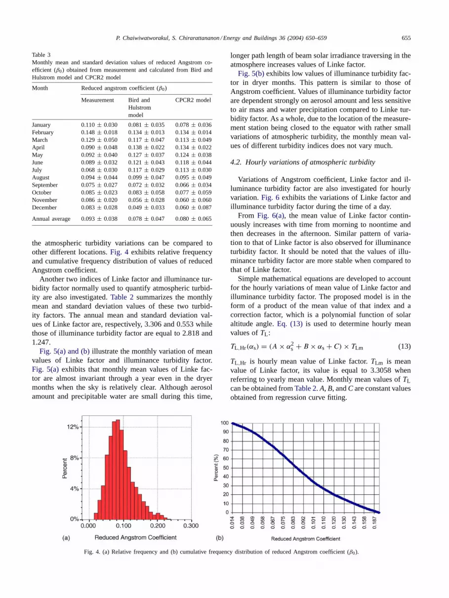
the atmospheric turbidity variations can be compared toother different locations.Fig. 4 exhibits relative frequencyand cumulative frequency distribution of values of reducedAngstrom coefficient.

Another two indices of Linke factor and illuminance tur-bidity factor normally used to quantify atmospheric turbid-ity are also investigated.Table 2summarizes the monthlymean and standard deviation values of these two turbid-ity factors. The annual mean and standard deviation val-ues of Linke factor are, respectively, 3.306 and 0.553 whilethose of illuminance turbidity factor are equal to 2.818 and1.247.

Fig. 5(a) and (b)illustrate the monthly variation of meanvalues of Linke factor and illuminance turbidity factor.Fig. 5(a)exhibits that monthly mean values of Linke fac-tor are almost invariant through a year even in the dryermonths when the sky is relatively clear. Although aerosolamount and precipitable water are small during this time,

Fig. 4. (a) Relative frequency and (b) cumulative frequency distribution of reduced Angstrom coefficient (β0).

longer path length of beam solar irradiance traversing in theatmosphere increases values of Linke factor.

Fig. 5(b)exhibits low values of illuminance turbidity fac-tor in dryer months. This pattern is similar to those ofAngstrom coefficient. Values of illuminance turbidity factorare dependent strongly on aerosol amount and less sensitiveto air mass and water precipitation compared to Linke tur-bidity factor. As a whole, due to the location of the measure-ment station being closed to the equator with rather smallvariations of atmospheric turbidity, the monthly mean val-ues of different turbidity indices does not vary much.

4.2. Hourly variations of atmospheric turbidity

Variations of Angstrom coefficient, Linke factor and il-luminance turbidity factor are also investigated for hourlyvariation.Fig. 6 exhibits the variations of Linke factor andilluminance turbidity factor during the time of a day.

From Fig. 6(a), the mean value of Linke factor contin-uously increases with time from morning to noontime andthen decreases in the afternoon. Similar pattern of varia-tion to that of Linke factor is also observed for illuminanceturbidity factor. It should be noted that the values of illu-minance turbidity factor are more stable when compared tothat of Linke factor.

Simple mathematical equations are developed to accountfor the hourly variations of mean value of Linke factor andilluminance turbidity factor. The proposed model is in theform of a product of the mean value of that index and acorrection factor, which is a polynomial function of solaraltitude angle.Eq. (13) is used to determine hourly meanvalues ofTL:

TL,Hr(αs) = (A × α2s + B × αs + C) × TLm (13)

TL,Hr is hourly mean value of Linke factor.TLm is meanvalue of Linke factor, its value is equal to 3.3058 whenreferring to yearly mean value. Monthly mean values ofTLcan be obtained fromTable 2. A, B, andC are constant valuesobtained from regression curve fitting.


Fig. 5. Monthly variation of mean value of (a) Linke factor (TL ) and (b) illuminance turbidity factor (Til ).

Fig. 6. Hourly variations of mean value of (a) Linke factor (TL ) and (b) illuminance turbidity factor (Til ).

The proposed model for illuminance turbidity factor is inthe same for as that for the model of Linke factor. Illumi-nance turbidity factor would be calculated by another set ofparametersA, B, C and replacingTL,Hr and TLm by Til ,Hrand Tilm . The yearly mean value of illuminance turbidityfactor is 2.8181. Using regression, the resulting values ofcoefficientsA, B, andC are listed inTable 4.

Fig. 7(a) and (b)exhibit hourly mean values of Linke fac-tor and illuminance turbidity factor and their correspondingvalues obtained from the proposed model plotted againstsolar altitude angle. Comparing to the measured values, rel-

Table 4Values of coefficientsA, B, and C of Eq. (13) for determining hourlymean values of Linke factor and illuminance turbidity factor

Turbidity indices A B C R2

Linke factor −0.00009 0.01350 0.54307 0.952Illuminance turbidity factor −0.00015 0.01997 0.37168 0.910

atively low values of Linke factor and illuminance turbidityfactor are obtained from the proposed models at low solaraltitude angle. Higher values of beam normal irradianceand illuminance at low altitude angles are expected whenthe models are used.

4.3. Correlation among Angstrom coefficient, Linke factorand illuminance turbidity factor

Correlation between Angstrom coefficient, Linke factorand illuminance turbidity factor are investigated. Values ofAngstrom coefficient are plotted against values of Linkefactor and illuminance turbidity factor. FromFig. 8(a)and (b), linear relationship is suggested to correlate valueof Angstrom turbidity coefficient with those of the othertwo turbidity indices. The mathematical model proposed isthus in form

β0 = D + ETL (14)


Fig. 7. Plot of hourly mean value of (a) Linke factor (TL ) and (b) illuminance turbidity factor (Til ) obtained from measurement and the use of theproposed model.

Fig. 8. Plots of reduced Angstrom coefficient against Linke factor and illuminance turbidity factor. Scattered plot of (a)TL againstβ0; (b) Til againstβ0.

whereD andE are constant values obtained from regressioncurve fitting.

Values of coefficientsD and E obtained for linear re-gression are listed inTable 5. Low accuracy (low valueof coefficient of correlation) is obtained when values ofLinke factor are used to calculate the corresponding valuesof Angstrom coefficient. Large scattering is obvious in theplot of Angstrom coefficient values against Linke factor val-ues. The plot demonstrates that Linke factor depends on theamount of water precipitation in the atmosphere.

Table 5Constant values of coefficientsD andE of Eq. (14)for determining valueof Angstrom coefficient from Linke factor and illuminance turbidity factor

Turbidity indices D E R2

Linke factor −0.0714 0.0495 0.540Illuminance turbidity factor −0.0300 0.0404 0.700

Because water vapor absorption occurs predominantly inthe infrared band, illuminance turbidity factor is insensitiveto amount of water vapor. In addition, because illuminancestrongly occupies a narrow band of solar wavelengths, theextinction coefficient is relatively insensitive to air mass.Strong linear relationship of Angstrom coefficient and illu-minance turbidity factor is confirmed fromFig. 8(b).

4.4. Calculation of direct normal irradiance andilluminance

Beam normal irradiance and illuminance can be computedfrom Bouguer–Lambert law. One important information isturbidity of the prevailing sky which can be quantified byLinke factor and illuminance turbidity factor.

Values of beam normal irradiance are computed usingEq. (3). Values of Linke factor used in the calculation areobtained from two different methods:


Table 6Comparison of discrepancy of measured and calculated values of beamnormal irradiance obtained from Method A and Method B

Data Mean (W/m2

or klux)MBD (W/m2

or klux)RMSD (W/m2

or klux)

Beam normal irradianceMeasurement 839.02 – –Method A 833.92 −5.10 63.23Method B 840.13 1.11 59.10

Beam normal illuminanceMeasurement 93.78 – –Method A 92.51 1.27 7.67Method B 93.49 0.29 7.42

Method A: monthly mean values of Linke factor fromTable 2, and

Method B: monthly mean values of Linke factor fromTable 2incorporating with the proposed model for com-puting hourly mean values of Linke factor.

Similar procedure is also used for beam normal illumi-nance. Two statistical estimators of mean bias difference(MBD) and root mean square difference (RMSD) are usedto evaluate the accuracy of the models. The two estimatorsare different in nature and can give different results. RMSDgives more weight to points far away from the mean. RMSDgive only positive values. MBD can give positive or nega-tive values, with positive value implying an overestimationof the model. The definition of mean bias difference (MBD)and root mean square difference (RMSD) can be expressedby the following equations:

MBD =∑N

i=1(Ci − Mi)

Nand

RMSD=√∑N

i=1(Ci − Mi)2

N(15)

where the units are in W/m2 for irradiance and in lux forilluminance.

Table 6exhibits the comparison of the values of beamnormal irradiance and illuminance obtained from Method Aand Method B and those obtained from measurement. It isobvious that the values of computed beam normal irradianceobtained from Method B are much closer to the values ofbeam normal irradiance obtained from measurement thanthose obtained from Method A.

5. Conclusion

The turbidity indices, namely, Linke factor, Angstrom co-efficient, and illuminance turbidity factor have been derivedfrom the record of two and half-year measurement at theAIT solar and daylight monitoring station. The mean valuesand frequency of occurrence of each index have been usedto characterize the atmospheric turbidity of Thai sky. Values

of the turbidity of the atmosphere are found to vary withseasons, months and hours.

The results show that the skies on cloudless days are cleanand clear. Atmospheric turbidity is low and quite stable dur-ing dryer months and increases in wet season from Marchto August. The turbidity of the sky also varies with time ofday. The turbidity increases from morning to noontime andthen decreases in the afternoon. The annual mean valuesof Angstrom coefficient, wavelength exponent, Linke factorand illuminance turbidity factor are 0.098, 1.272, 3.306 and2.818, respectively.

Linear function has been used to correlate the index ofAngstrom coefficient with the other two indices which areLinke factor and illuminance turbidity factor. Illuminanceturbidity factor strongly correlates with Angstrom coeffi-cient. The results also demonstrate that illuminance turbid-ity factor is insensitive to the amount of water vapor in theatmosphere.

Simple polynomial function has been developed to modelthe hourly variations of Linke factor and illuminance turbid-ity factor as a function of solar altitude angle and its meanvalues. Using the Bouguer–Lambert law incorporating thevalues of Linke factor and illuminance turbidity factor ob-tained from the models developed, the values of beam nor-mal irradiance and illuminance can be calculated precisely.Accurate model of beam illuminance is useful in design fordaylighting for energy conservation in buildings. Accuratemodel of beam irradiance can be used in building energysimulation studies.

Acknowledgements

This paper reports a part of a work in a project set up toconduct research on daylighting. The project is supported bythe National Energy Conservation Promotion Fund whichis administered by the National Energy Policy Office of theRoyal Thai Government.

References

[1] S. Chirarattananon, P. Chaiwiwatworakul, S. Pattanasethanon, Day-light availability and models for global and diffuse horizontal illumi-nance and irradiance for Bangkok, Renewable Energy 26 (1) (2002)69–89.

[2] C. Gueymard, Analysis of monthly average atmospheric precipitablewater and turbidity in Canada and Northern United States, SolarEnergy 53 (1) (1994) 57–71.

[3] C. Gueymard, J.D. Garrison, Critical evaluation of precipitable waterand atmospheric turbidity in Canada using measured hourly solarirradiance, Solar Energy 62 (4) (1998) 291–307.

[4] C. Gueymard, F. Vignola, Determination of atmospheric turbidityfrom the diffuse-beam broadband irradiance ratio, Solar Energy 63 (3)(1998) 135–146.

[5] M. Katz, A. Baille, M. Mermier, Atmospheric turbidity in a semi-ruralsite-I. Evaluation and comparison of different atmospheric turbiditycoefficients, Solar Energy 28 (4) (1982) 323–327.


[6] M. Katz, A. Baille, M. Mermier, Atmospheric turbidity in a semi-ruralsite-II. Influence of climatic parameters, Solar Energy 28 (4) (1982)329–334.

[7] J. Canada, J.M. Pinazo, J.V. Bosca, Determination of Angstromturbidity coefficient at Valencia, Renewable Energy 3 (6/7) (1993)621–626.

[8] C.P. Jacovides, C. Varotsos, N.A. Kaltsounides, Atmospheric turbidityparameters in the highly polluted site of Athens Basin, RenewableEnergy 4 (5) (1994) 465–470.

[9] J.M. Pinazo, J. Canada, J.V. Bosca, A new method to determineAngstrom’s turbidity coefficient: its application for Valencia, SolarEnergy 54 (4) (1995) 219–226.

[10] J.V. Bosca, J.M. Pinazo, J. Canada, V. Ruiz, Angstrom’s turbiditycoefficient in Seville Spain, in the years 1990 and 1991, InternationalJournal of Ambient Energy 17 (4) (1996) 171–178.

[11] M. Cucumo, D. Kaliakatsos, V. Marinelli, A calculation methodfor the estimation of the Linke turbidity factor, Renewable Energy19 (1/2) (2000) 249–258.

[12] M. Cucumo, V. Marinelli, G. Oliveti, Experimental data of the Linketurbidity factor and estimates of the Angstrom turbidity coefficientfor Tow Italian localities, Renewable Energy 17 (3) (1999) 390–410.

[13] A.S. Rapti, Atmospheric transparency, atmospheric turbidity and cli-mate parameters, Solar Energy 69 (2) (2000) 99–111.

[14] R. Kittler, S. Darula, Parameterization problems of the very brightcloudy sky conditions, Solar Energy 62 (2) (1998) 93–100.

[15] A. Mani, O. Chacko, N.V. Iyer, Atmospheric turbidity over Indiafrom solar radiation measurements, Solar Energy 14 (2) (1973) 185–195.

[16] A. Mani, O. Chacko, Attenuation of solar radiation in the atmosphere,Solar Energy 24 (4) (1980) 347–349.

[17] M. Hussain, S. Khatun, M.G. Rasul, Determination of atmosphericturbidity in Bangladesh, Renewable Energy 20 (3) (2000) 325–332.

[18] R.H.B. Exell, The water content and turbidity of the atmosphere inThailand, Solar Energy 20 (5) (1978) 429–430.

[19] Z.D. Adeyefa, B. Holmgren, J.A. Adedokun, Spectral solar radiationmeasurements and turbidity: comparative studies within tropical anda sub-arctic environment, Solar Energy 60 (1) (1997) 17–24.

[20] A. Angstrom, Techniques of determining the turbidity of the atmo-sphere, Tellus 13 (2) (1961) 214–223.

[21] A. Angstrom, The parameters of atmospheric turbidity, Tellus 16(1964) 64–75.

[22] C. Gueymard, in: Proceedings of 23rd American Solar Energy SocietyAnnual Conference, Updated Transmittance Functions for Use inFast Spectral Direct Beam Irradiance Models, San Jose, CA., 1994.

[23] E. Vigroux, Contribution a l’etude experimenttale de l’absorption del’oxone, Annales de Physics 8 (1953) 709.

[24] A.Q. Malik, Estimation of atmospheric ozone for Association ofSouth East Asian Nations (ASEAN) countries, Renewable Energy12 (2) (1997) 193–202.

[25] M. Navvab, M. Karayel, E. Ne’eman, S. Selkowitz, Analysis ofatmospheric turbidity for daylight calculations, Energy and Buildings6 (1984) 293–303.

[26] R. Perez, R. Seals, J. Michalsky, All-weather model for sky luminancedistribution-preliminary configuration and validation, Solar Energy50 (3) (1993) 235–245.

[27] A. Louche, M. Maurel, G. Simonnot, G. Peri, M. Iqbal, Determinationof angstrom turbidity coefficient from direct total solar irradiancemeasurements, Solar Energy 38 (2) (1987) 89–96.

[28] C. Gueymard, A two-band model for the calculation of clear skysolar irradiance, illuminance, and photosynthetically active radiationat the Earth’s surface, Solar Energy 43 (5) (1989) 253–265.

Documents

An investigation of atmospheric turbidity of Thai sky