Estimation of atmospheric turbidity over Ghardaıa city

D. Djafera, A. Irbahb

aUnite de Recherche Appliquee en Energies Renouvelables, URAER, Centre de Developpement des Energies Renouvelables, CDER, 47133, Ghardaıa,AlgeriabLaboratoire Atmospheres, Milieux, Observations Spatiales (LATMOS), CNRS : UMR8190 - Universite Paris VI - Pierre et Marie Curie - Universite de Versailles

Saint-Quentin-en-Yvelines - INSU, 78280, Guyancourt, France

Abstract

The atmospheric turbidity expresses the attenuation of the solar radiation that reaches the Earth’s surface under cloudless sky and

describes the optical thickness of the atmosphere. We investigate the atmospheric turbidity over Ghardaıa city using two turbidity

parameters, the Linke turbidity factor and the Angstrom turbidity coefficient. Their values and temporal variation are obtained from

data recorded between 2004 and 2008 at Ghardaıa. The results show that both parameters have the same trend along the year. They

reach their maximum around summer months and their minimum around winter months. The monthly average value varies between

1.3 and 5.6 for the Linke turbidity factor and between 0.02 and 0.19 for the Angstrom turbidity coefficient. We find that 39.8% of

the Linke turbidity factor values are less than 3, 47.5% are between 3 and 5 and only 12.7% are greater than 5. For the Angstrom

turbidity coefficient, 9.4% of the values are less than 0.02, 75.4% are between 0.02 and 0.15 and 15.2% exceed 0.15.

Keywords: solar radiation, turbidity parameters, Linke factor, Angstrom coefficient.

1. Introduction

The quality and quantity of the solar radiation in a given

ground site should be considered before installing solar en-

ergy conversion systems. Photovoltaic and solar thermal energy

systems are usually designed considering their performance in

standard test conditions and without taking into account local

atmospheric ones (Malik, 2000). The reason is often the non-

availability of atmospheric data for a specific location when the

solar systems are designed. It is nevertheless essential that vari-

ations of solar cell/module efficiency in various atmospheric

turbidity and weather conditions are known to optimize their

performances since an increase in turbidity reduces the output

current of solar cells (Malik, 2000). Solar irradiance at ground

level is strongly dependent on the Earth’s atmosphere. Its con-

stituents (aerosols, water vapor, ...etc) absorb and diffuse sig-

nificantly the direct solar radiation. Thus, it is important to

quantify their temporal effects when recording solar radiation

measurements in a local area. This will helps in the future to

establish models and accurately estimate the clear sky radiation.

Among several turbidity parameters, the most frequently used

are the Linke turbidity factor (Linke, 1922) and the Angstrom

turbidity coefficient (Angstrom, 1961). As already mentioned

before, the knowledge of these turbidity parameters is impor-

tant to optimize the performances of solar radiation devices

installed at a particular location but it is also important (i) in

climate modeling and in pollution studies (Trabelsi and Mas-

moudi, 2011), (ii) to predict the availability of solar energy

∗Principal corresponding author∗∗Corresponding author

Email addresses: djdjafer@gmail.com (D. Djafer ),

air@latmos.ipsl.fr (A. Irbah )

under cloudless skies essential for the design of solar thermal

power plants and other solar energy conversion devices with

concentration systems, (iii) to compute the amount of spectral

global irradiance for the design of photovoltaic systems and cal-

culation of the photosynthetic energy for plant growth (Malik,

2000).

In the present work, we will use five years of data daily recorded

between 2004 and 2008 to study the turbidity of the atmosphere

over Ghardaıa city. It is the first time to our knowledge that this

kind of data and results covering a long period are presented for

this particular region. We will recall at first the definition of the

Linke turbidity factor and the Angstrom turbidity coefficient.

We will then present the data used for this study and discuss the

obtained results.

2. The Linke turbidity factor

The Linke turbidity factor Tl has been used since 1922 to

quantify atmospheric turbidity conditions. It is defined as the

number of clean dry atmospheres necessary to have the same

attenuation of the extraterrestrial radiation produced by the real

atmosphere (Trabelsi and Masmoudi, 2011). The Linke tur-

bidity factor is useful for modeling the atmospheric absorption

and scattering of the solar radiation during clear skies. The

Linke factor depends on the air mass and most popular meth-

ods normalize the measured values of Tl to an air mass equal to

2 (Grenier et al., 1994, Kasten, 1988). This turbidity factor de-

scribes the optical thickness of the atmosphere due to both the

absorption and scattering by the water vapor and aerosol parti-

cles relatively to a dry and clean atmosphere. It expresses the at-

mosphere turbidity or equivalently the attenuation of the direct

solar radiation flux. The value of the Linke factor may then be

Preprint submitted to Atmospheric Research March 12, 2013

*Manuscript

Click here to view linked References

derived from the direct component of the solar irradiance (Chai-

wiwatworakul et al., 1994, Ellouz et al., 2004, Mavromatakis

and Franghiadakis, 2007, Trabelsi and Masmoudi, 2011, Zakey

et al., 2004). Typical values of the Linke factor vary between

1 and 10. High values of the Linke factor mean that the so-

lar radiations are more attenuated in a clear sky atmosphere.

We use the following Equation to calculate the Linke factor

Tl (Mavromatakis and Franghiadakis, 2007, Trabelsi and Mas-

moudi, 2011):

Tl = Tlk

1δRa(ma)

1δRk(ma)

(1)

Tlk is the Linke factor according to Kasten (Kasten, 1980),

δRk(ma) the Rayleigh integral optical thickness and δRa(ma) the

integral optical thickness given by Louche et al. (1986) and ad-

justed by Kasten (1996). The subscript k stands for the au-

thor ”Kasten” and the subscript a for the word ”adjusted”. The

Linke factor Tlk is related to the normal incidence solar irradi-

ance by the Equation (Kasten, 1980, Trabelsi and Masmoudi,

2011):

Tlk =(

0.9 + 9.4 sin(h))

∗

(

2 ln(

I0(R0

R))

− ln(In)

)

(2)

where h is the Sun’s elevation angle in degrees, In the direct nor-

mal solar irradiance at normal incidence and I0 the solar con-

stant (1367W/m2). R and R0 are respectively the instantaneous

and mean Sun-Earth distances. The value of In is measured di-

rectly through a pyrheliometer in (W/m2).

The expression of δRk(ma) and δRa(ma) are given by the follow-

ing Equations:

1

δRa(ma) = 6.6296 + 1.7513ma − 0.1202m2

a

+0.0065m3a − 0.00013m4

a (3)

1

δRk(ma) = 9.4 + 0.9ma (4)

where ma is the air mass given by:

ma = mr

(

P

101325

)

(5)

The parameter mr is the air mass at the standard conditions

(Canada et al., 1993) defined by:

mr = [sin(h) + 0.15(3.885+ h)−1.253]−1 (6)

The local pressure P (in Pascal) is given by (Pinazo et al.,

1995):

P = 101325 exp(−0.0001184z) (7)

where z is the altitude in meter of the location above sea level.

3. The Angstrom coefficient

The Angstrom coefficient β is a measure of the presence of

aerosols. It characterizes the amount of aerosol content in the

vertical column of air with transversal unitary (Trabelsi and

Masmoudi, 2011). The typical values of this parameter vary be-

tween 0 to 0.5 (Angstrom, 1961, 1964, Danny and Lam, 2002,

Grenier et al., 1995, Gueymard and Garrison, 1998, Trabelsi

and Masmoudi, 2011). Its minimum value (zero) refers to an

ideally dust free atmosphere, while values superior to unity re-

fer to an extremely turbid atmosphere. The Angstrom coef-

ficient can be determined with different methods and spectral

measurements (Jacovides et al., 2005, Kaskaoutis et al., 2008a,

Kaskaoutis and Kambezidis, 2008b, Lopez and Batlles, 2004,

Masmoudi et al., 2003, Trabelsi and Masmoudi, 2011, Zakey

et al., 2004). We will compute the Angstrom coefficient using

the empirical formula of Dogniaux (1974) since we have not a

photometric instrument at Ghardaıa to discriminate aerosols by

mean of spectral measurements. Many authors have used this

formula to derive the Angstrom turbidity coefficient (Cucumo

et al., 1999, Danny and Lam, 2002, Grenier et al., 1995, Janjai

et al., 2003, Lopez and Batlles, 2004, Vida et al., 1999). This

empirical formula is given by the following Equation:

β =

Tl −

[

h+8539.5 exp(−wp)+47.4

+ 0.1

]

16 + 0.22wp(8)

where h is the Sun’s elevation angle in degrees and wp the pre-

cipitation amount in centimeter. The value of wp is calculated

using the Equation (Leckner, 1978):

wp = 0.493φ

Texp

(

26.23 −5416

T

)

(9)

where T is the temperature in Kelvin and φ is the relative hu-

midity in fractions of one.

Other models exist to calculate the Angstrom coefficient such

as the models of Louche et al. (1986), of Pinazo et al. (1995)

and of Gueymard and Vignola (1998). These models require

some parameters that we have not at Ghardaıa for the period

considered in this study. Such parameters are the wavelength

exponent α that is used to calculate the aerosol transmittance,

the ground albedo ρg, the forward scattering Fc and the single

scattering albedo w0. Wen and Yeh (2009) have studied the at-

mospheric turbidity properties of Taichung Harbor considering

data recorded in 2004-2005 and the Angstrom turbidity models

of Louche et al. (1986) and Pinazo et al. (1995). They found

that the annual mean values of the Angstrom turbidity coeffi-

cient obtained from theses models were respectively 0.174 and

0.21.

4. Site location and solar radiation data

The data used to perform the present study have been

recorded at the Applied Research Unit for Renewable Energies

(URAER) situated in the south of Algeria far from Ghardaıa

city of about 18 km. The latitude, longitude and altitude of the

2

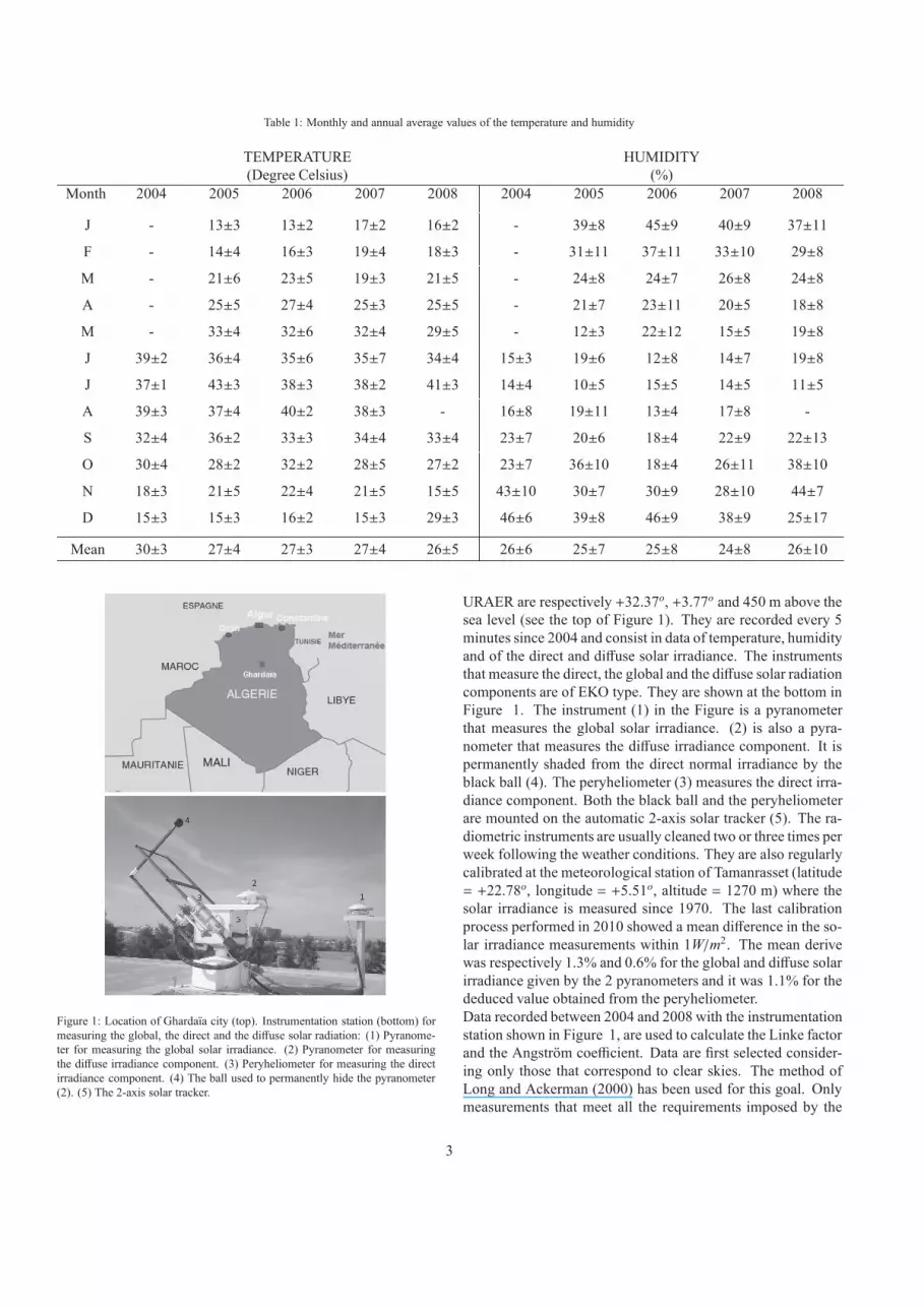
Table 1: Monthly and annual average values of the temperature and humidity

TEMPERATURE HUMIDITY

(Degree Celsius) (%)

Month 2004 2005 2006 2007 2008 2004 2005 2006 2007 2008

J - 13±3 13±2 17±2 16±2 - 39±8 45±9 40±9 37±11

F - 14±4 16±3 19±4 18±3 - 31±11 37±11 33±10 29±8

M - 21±6 23±5 19±3 21±5 - 24±8 24±7 26±8 24±8

A - 25±5 27±4 25±3 25±5 - 21±7 23±11 20±5 18±8

M - 33±4 32±6 32±4 29±5 - 12±3 22±12 15±5 19±8

J 39±2 36±4 35±6 35±7 34±4 15±3 19±6 12±8 14±7 19±8

J 37±1 43±3 38±3 38±2 41±3 14±4 10±5 15±5 14±5 11±5

A 39±3 37±4 40±2 38±3 - 16±8 19±11 13±4 17±8 -

S 32±4 36±2 33±3 34±4 33±4 23±7 20±6 18±4 22±9 22±13

O 30±4 28±2 32±2 28±5 27±2 23±7 36±10 18±4 26±11 38±10

N 18±3 21±5 22±4 21±5 15±5 43±10 30±7 30±9 28±10 44±7

D 15±3 15±3 16±2 15±3 29±3 46±6 39±8 46±9 38±9 25±17

Mean 30±3 27±4 27±3 27±4 26±5 26±6 25±7 25±8 24±8 26±10

Figure 1: Location of Ghardaıa city (top). Instrumentation station (bottom) for

measuring the global, the direct and the diffuse solar radiation: (1) Pyranome-

ter for measuring the global solar irradiance. (2) Pyranometer for measuring

the diffuse irradiance component. (3) Peryheliometer for measuring the direct

irradiance component. (4) The ball used to permanently hide the pyranometer

(2). (5) The 2-axis solar tracker.

URAER are respectively +32.37o, +3.77o and 450 m above the

sea level (see the top of Figure 1). They are recorded every 5

minutes since 2004 and consist in data of temperature, humidity

and of the direct and diffuse solar irradiance. The instruments

that measure the direct, the global and the diffuse solar radiation

components are of EKO type. They are shown at the bottom in

Figure 1. The instrument (1) in the Figure is a pyranometer

that measures the global solar irradiance. (2) is also a pyra-

nometer that measures the diffuse irradiance component. It is

permanently shaded from the direct normal irradiance by the

black ball (4). The peryheliometer (3) measures the direct irra-

diance component. Both the black ball and the peryheliometer

are mounted on the automatic 2-axis solar tracker (5). The ra-

diometric instruments are usually cleaned two or three times per

week following the weather conditions. They are also regularly

calibrated at the meteorological station of Tamanrasset (latitude

= +22.78o, longitude = +5.51o, altitude = 1270 m) where the

solar irradiance is measured since 1970. The last calibration

process performed in 2010 showed a mean difference in the so-

lar irradiance measurements within 1W/m2. The mean derive

was respectively 1.3% and 0.6% for the global and diffuse solar

irradiance given by the 2 pyranometers and it was 1.1% for the

deduced value obtained from the peryheliometer.

Data recorded between 2004 and 2008 with the instrumentation

station shown in Figure 1, are used to calculate the Linke factor

and the Angstrom coefficient. Data are first selected consider-

ing only those that correspond to clear skies. The method of

Long and Ackerman (2000) has been used for this goal. Only

measurements that meet all the requirements imposed by the

3

0 100 200 3001

5

8

date(days)

Tl

0 100 200 3001

5

8

date(days)

Tl

0 100 200 3001

5

8

date(days)

Tl

0 100 200 3001

5

8

date(days)

Tl

0 100 200 3001

5

8

date(days)

Tl

2 4 6 8 10 12

2

4

6

date(month)

Tl

2 4 6 8 10 12

2

4

6

date(month)

Tl

2 4 6 8 10 12

2

4

6

date(month)

Tl

2 4 6 8 10 12

2

4

6

date(month)

Tl

2 4 6 8 10 12

2

4

6

date(month)

Tl

2004

2005

2006

2007

2008

Figure 2: Daily (left part) and monthly (right part) variations of the Linke tur-

bidity factor Tink with the error bars.

four successive tests of the method are considered. 37% of the

whole data set remains finally for the present study when ap-

plying the selection.

For the meteorological data, only the temperature and the

humidity data are available for the considered period. The

monthly and the annual average values of these two meteoro-

logical parameters are summarized in Table 1. We note that

the annual average values of the temperature and humidity are

respectively 27o and 25%. The monthly average values are be-

tween 13o and 43o for the temperature and between 10% and

46% for the humidity. The predominant wind direction over

Ghardaıa city is South-West according to information given by

a meteorological station located at about 200 meters of our site.

5. Results and discussion

We use Equations (1) and (8) to calculate the Linke turbidity

factor and the Angstrom turbidity coefficient. Some algorithms

were needed and developed to determine the ephemerides nec-

essary to perform these calculations. The monthly and the an-

nual average values of the Linke factor and the Angstrom co-

efficient are given in Table 2. The daily and monthly varia-

tions of these two parameters are shown in Figures 2 and 3.

We can note that they show the same trend along the year and

have their maximum and minimum values respectively during

the summer and winter months. This can be explained by a hot

summer climate and winds of the south sectors (Sirocco) that

150 200 250 300 3500

0.1

0.2

date(days)

β

0 100 200 3000

0.1

0.2

date(days)

β

0 100 200 3000

0.1

0.2

date(days)

β

0 100 200 3000

0.1

0.2

date(days)

β

0 100 200 3000

0.1

0.2

date(days)

β

6 8 10 120

0.1

0.2

date(month)

β

2 4 6 8 10 120

0.1

0.2

date(month)

β

2 4 6 8 10 120

0.1

0.2

date(month)

β

2 4 6 8 10 120

0.1

0.2

date(month)

β

2 4 6 8 10 120

0.1

0.2

date(month)

β

2004

2007

2008

2006

2005

Figure 3: Daily (left part) and monthly (right part) variations of the Angstrom

coefficient β with the error bars.

characterize the region of Ghardaıa. This kind of winds brings

particles of dust and sand with them, which leads to increase the

Linke factor and the Angstrom coefficient (Bouhadda and Ser-

rir, 2009). The period of winter is characterized by rains that

wash the atmosphere and thus contribute to diminish both tur-

bidity variables. In fact, the monthly average of rainfall amount

2004 2005 2006 2007 2008 20090

1

2

3

4

5

6

7

8

9

date (years)

Linke

turb

idity

facto

r (T l)

2004 2005 2006 2007 2008 20090

0.05

0.1

0.15

0.2

0.25

0.3

0.35

0.4

0.45

date (years)

Angs

trom

tubid

ity co

effic

ient (

β)

Figure 4: Seasonal variation of the Linke turbidity factor (left part) and the

Angstrom turbidity coefficient (right part). The points are the daily variations

while the circles are the monthly ones.

4

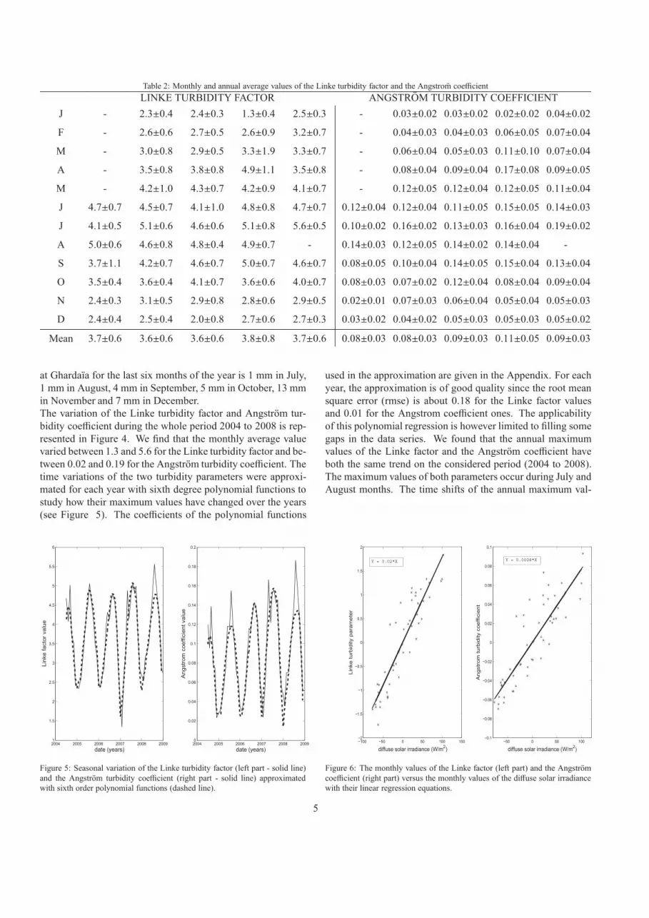
Table 2: Monthly and annual average values of the Linke turbidity factor and the Angstrom coefficient

LINKE TURBIDITY FACTOR ANGSTROM TURBIDITY COEFFICIENT

J - 2.3±0.4 2.4±0.3 1.3±0.4 2.5±0.3 - 0.03±0.02 0.03±0.02 0.02±0.02 0.04±0.02

F - 2.6±0.6 2.7±0.5 2.6±0.9 3.2±0.7 - 0.04±0.03 0.04±0.03 0.06±0.05 0.07±0.04

M - 3.0±0.8 2.9±0.5 3.3±1.9 3.3±0.7 - 0.06±0.04 0.05±0.03 0.11±0.10 0.07±0.04

A - 3.5±0.8 3.8±0.8 4.9±1.1 3.5±0.8 - 0.08±0.04 0.09±0.04 0.17±0.08 0.09±0.05

M - 4.2±1.0 4.3±0.7 4.2±0.9 4.1±0.7 - 0.12±0.05 0.12±0.04 0.12±0.05 0.11±0.04

J 4.7±0.7 4.5±0.7 4.1±1.0 4.8±0.8 4.7±0.7 0.12±0.04 0.12±0.04 0.11±0.05 0.15±0.05 0.14±0.03

J 4.1±0.5 5.1±0.6 4.6±0.6 5.1±0.8 5.6±0.5 0.10±0.02 0.16±0.02 0.13±0.03 0.16±0.04 0.19±0.02

A 5.0±0.6 4.6±0.8 4.8±0.4 4.9±0.7 - 0.14±0.03 0.12±0.05 0.14±0.02 0.14±0.04 -

S 3.7±1.1 4.2±0.7 4.6±0.7 5.0±0.7 4.6±0.7 0.08±0.05 0.10±0.04 0.14±0.05 0.15±0.04 0.13±0.04

O 3.5±0.4 3.6±0.4 4.1±0.7 3.6±0.6 4.0±0.7 0.08±0.03 0.07±0.02 0.12±0.04 0.08±0.04 0.09±0.04

N 2.4±0.3 3.1±0.5 2.9±0.8 2.8±0.6 2.9±0.5 0.02±0.01 0.07±0.03 0.06±0.04 0.05±0.04 0.05±0.03

D 2.4±0.4 2.5±0.4 2.0±0.8 2.7±0.6 2.7±0.3 0.03±0.02 0.04±0.02 0.05±0.03 0.05±0.03 0.05±0.02

Mean 3.7±0.6 3.6±0.6 3.6±0.6 3.8±0.8 3.7±0.6 0.08±0.03 0.08±0.03 0.09±0.03 0.11±0.05 0.09±0.03

at Ghardaıa for the last six months of the year is 1 mm in July,

1 mm in August, 4 mm in September, 5 mm in October, 13 mm

in November and 7 mm in December.

The variation of the Linke turbidity factor and Angstrom tur-

bidity coefficient during the whole period 2004 to 2008 is rep-

resented in Figure 4. We find that the monthly average value

varied between 1.3 and 5.6 for the Linke turbidity factor and be-

tween 0.02 and 0.19 for the Angstrom turbidity coefficient. The

time variations of the two turbidity parameters were approxi-

mated for each year with sixth degree polynomial functions to

study how their maximum values have changed over the years

(see Figure 5). The coefficients of the polynomial functions

2004 2005 2006 2007 2008 20091

1.5

2

2.5

3

3.5

4

4.5

5

5.5

6

date (years)

Lin

ke f

acto

r valu

e

2004 2005 2006 2007 2008 20090

0.02

0.04

0.06

0.08

0.1

0.12

0.14

0.16

0.18

0.2

date (years)

Angstr

om

coeff

icie

nt

valu

e

Figure 5: Seasonal variation of the Linke turbidity factor (left part - solid line)

and the Angstrom turbidity coefficient (right part - solid line) approximated

with sixth order polynomial functions (dashed line).

used in the approximation are given in the Appendix. For each

year, the approximation is of good quality since the root mean

square error (rmse) is about 0.18 for the Linke factor values

and 0.01 for the Angstrom coefficient ones. The applicability

of this polynomial regression is however limited to filling some

gaps in the data series. We found that the annual maximum

values of the Linke factor and the Angstrom coefficient have

both the same trend on the considered period (2004 to 2008).

The maximum values of both parameters occur during July and

August months. The time shifts of the annual maximum val-

−100 −50 0 50 100 150−2

−1.5

−1

−0.5

0

0.5

1

1.5

2

diffuse solar irradiance (W/m2)

Lin

ke t

urb

idity p

ara

mete

r

−50 0 50 100−0.1

−0.08

−0.06

−0.04

−0.02

0

0.02

0.04

0.06

0.08

0.1

diffuse solar irradiance (W/m2)

Angstr

om

turb

idity c

oeff

icie

nt

Y = 0.0008*X Y = 0.02*X

Figure 6: The monthly values of the Linke factor (left part) and the Angstrom

coefficient (right part) versus the monthly values of the diffuse solar irradiance

with their linear regression equations.

5

ues have also been studied considering the middle of the year

as reference (July, 1st). We found time shifts up to 2 months

during the period 2004 to 2008. Moreover, the correlation of

the two turbidity parameters with the diffuse solar irradiance is

analyzed. We can observe a strong correlation between them as

shown in Figure 6 where we have plotted the monthly values of

the Linke factor and the Angstrom coefficient versus the diffuse

solar irradiance. Their mean value has been subtracted leading

to directly deduce the correlation factor from the slope of the

fitted straight line in the curves. We find a correlation factor of

0.92 between the Linke factor and the diffuse solar irradiance

and 0.87 for the Angstrom coefficient.

We have finally performed a statistical analysis by comput-

ing the histograms of the values of the Linke turbidity factor

and of the Angstom coefficient. They are shown in Figure 7

where we can notice that 39.8% of the Linke turbidity factor

values are less than 3, 47.5% are between 3 and 5 and only

12.7% are greater than 5. For the Angstrom turbidity coeffi-

cient, 9.4% of the values are less than 0.02, 75.4% are between

0.02 and 0.15 and 15.2% exceed 0.15. We have compared our

results with those obtained by Trabelsi and Masmoudi (2011)

who studied the atmospheric turbidity over the city of Sidi Bou

Saıd in Tunisia (latitude +36.87o, longitude +10.35o, altitude:

130 m). It is at a latitude approaching that of Ghadaıa but lo-

cated at a lower altitude. Trabelsi and Masmoudi used the same

method as our to compute the two turbidity parameters taking

data recorded on the site between July 2008 and June 2009.

They showed that about 68% of the Angstrom coefficient val-

ues ranged between 0.02 and 0.1 and 7% of the values were

greater than 0.15. For the Linke factor, 66% of the values were

between 3 and 5 and only 27% of them were greater than 5. We

may notice that the results are similar with ours but with a tur-

bidity lower in Ghardaıa city. It should be noted however, that

only one year of measurements was used to perform the turbid-

ity analysis at Sidi Bou Saıd while we have considered a period

of five years in our study.

6. Conclusion

Five years of data recorded between 2004 and 2008 at the

URAER (Applied Research Unit for Renewable Energies) were

used to study the turbidity of the atmosphere over the region of

Ghardaıa by means of two parameters, the Linke turbidity fac-

tor and the Angstrom coefficient. The results reveal that the two

parameters have the same behavior along the year. A maximum

attenuation by the Earth’s atmosphere of the solar radiations

recorded at the ground level is observed in summer and recip-

rocally a minimum in winter. This seasonal trend is related to

the climate of the region which is characterized in summer by

a hot weather and Sirocco winds that bring dust and sand parti-

cles and in winter by a dry weather and rains. The occurrence

date of the annual maximum values of both turbidity parame-

ters change however over the years. The time shift may be up to

2 months relatively to the middle of the year (July 1st). We find

also that the monthly parameter values are strongly correlated

with the diffuse solar irradiance. The results we obtain for the

0 2 4 6 8 100

20

40

60

80

100

120

140

160

180

Linke turbidity factor (Tl)

occure

nce

0 0.1 0.2 0.3 0.4 0.50

20

40

60

80

100

120

140

160

180

200

Angstrom turbidity coefficient (β)

occure

nce

Figure 7: Histogram of the values of the Linke factor (left part) and the

Angstrom coefficient (right part) obtained on a period of the five years.

Linke turbidity factor and the Angstrom coefficient at Ghardaıa,

have been compared with those deduced from a similar study

performed over the Sidi Bou Saıd city in Tunisia. We find re-

sults very close but with lower turbidity conditions at Ghardaıa.

The analysis period considered for the Sidi Bou Saıd study is

however only one year.

The present study is a preliminary work that asks now for de-

veloping models to better explain the obtained results for the

Ghardaıa region and to understand the evolution of both the

Linke factor and the Angstrom coefficient during a long time

period. We need also to analyze how the used models may af-

fect the estimation of the two parameters. Nevertheless, the

results of both parameters reported in the present paper may be

used to (i) design and check the performance of solar devices of

any locality that have a similar climate to Ghardaıa, (ii) to in-

vestigate/study the variation of efficiency of solar devices with

the variation in the spectrum of incident radiation, (iii) to have a

reference point for global studies of the evolution of atmosphere

turbidity and aerosols.

Acknowledgements

We would like to thank and acknowledge the support of the

team at the Research Unit on Renewable Energies of Ghardaıa

whose collected the data used in the present study.

References

Angstrom A., 1961. Techniques of determining the turbidity of the atmosphere.

Tellus 13, 214-223.

Angstrom A., 1964. The parameters of atmospheric turbidity. Tellus 16, 64-75.

Bouhadda Y. and Serrir L., 2006. Contribution a l’etude du trouble atmo-

spherique de Linke sur le site de Ghardaıa. Revue des Energies Renouve-

lables 9, 277-284.

Canada J., Pinazo J.M. and Bosca, J.V, 1993. Determination of Angstrom’s

turbidity coefficient at Valencia. Renewable Energy 3, 6/7, 621-626.

Chaiwiwatworakul P. and Chirarattananon, S., 2004. An investigation of atmo-

spheric turbidity of Thai sky. Energy and Buildings 36, 650-659.

6

Table 3: Coefficients of the sixth order polynomial function for the Linke turbidity factor

Year a6 a5 a4 a3 a2 a1 a0

2004 0 0 0 5.327e+01 -3.204e+05 6.423e+08 -4.292e+11

2005 1.475e-06 -5.222e-03 3.574e-02 -2.831e+04 2.326e+08 -4.575e+11 2.831e+14

2006 1.747e-06 -1.557e-02 4.190e+01 8.236e+03 -2.288e+08 3.857e+11 -2.060e+14

2007 1.005e-06 -7.663e-03 2.845e+01 -8.225e+04 1.825e+08 -2.335e+11 1.205e+14

2008 -1.263e-06 7.806e-03 -2.274e+01 7.239e+04 -2.101e+08 3.172e+11 -1.783e+14

Table 4: Coefficients of the sixth order polynomial function for the Angstrom turbidity coefficient

Year a6 a5 a4 a3 a2 a1 a0

2004 0 0 0 5.320e-01 -3.200e+03 6.417e+06 -4.289e+09

2005 0 0 0 -3.539e-01 2.129e+03 -4.268e+06 2.853e+09

2006 5.854e-09 -1.236e-04 3.084e-01 1.555e+03 -8.245e+06 1.322e+10 -7.254e+12

2007 0 0 0 -5.266e-01 3.171e+03 -6.364e+06 4.258e+09

2008 -6.825e-08 5.567e-04 -2.394e+00 7.832e+03 -1.770e+07 2.199e+10 -1.097e+13

Cucumo M., Marinelli V. and Oliveti G., 1999. Experimental data of the Linke

turbidity factor and estimates of the turbidity coefficient for two Italian lo-

calities. Renewable Energy 17, 397-410.

Danny H.W.Li and Joseph C.Lam., 2002. A study of atmosphere turbidity for

Honh Kong. Renewable Energy 25, 1-13.

Dogniaux R., 1974. Reprentations analytiques des composantes du ray-

onnement lumineux solaire. Conditions du ciel serein. Institut Royal de

Metiorologie de Belgique, Serie A No. 83, 3-24.

Ellouz F., Masmoud M. and Medhioub K., 2008. Study of the atmospheric

turbidity over Northern Tunisia. Renewable Energy 2, 1-5.

Grenier J. C., De La Casiniere A. and Cabot T., 1994. A spectral model of

Linke’s turbidity factor and its experimental implications. Solar Energy 52,

303-314.

Grenier J.C., Casiniere A. and Cabo T.T., 1995. Atmospheric turbidity analyzed

by means of standardized Linke’s factor. Journal of Applied Meteorology

34, 1449-1458.

Gueymard C.A. and Garrison J.D. (1998) Critical evaluation of precipitable

water and atmospheric turbidity in Canada using measured hourly solar ir-

radiance. Solar Energy 62 (4), 291-307.

Gueymard C. and Vignola F., 1998. Determination of atmospheric turbidity

from the diffuse-beam broadband irradiance ratio. Solar Energy 63 (3), 135-

146.

Jacovides C.P., Kaltsounides N.A., Assimakopoulos D.N. and Kaskaoutis D.G.,

2005. Spectral aerosol optical depth and Angstrom parameters in the pol-

luted Athens atmosphere. Theoretical and Applied Climatology 81, 161-

167.

Janjai S., Kumharn W. and Laksanaboonsong J., 2003. Determination of

Angstrom’s turbidity coefficient over Thailand. Renewable Energy 28, 1685-

1700.

Karayel M., Navvab M., Ne’eman E. and Selkowitz S., 1984. Zenith lumi-

nance and sky luminance distributions for daylighting calculations. Energy

and Buildings 6(3), 283-291.

Kaskaoutis D.G. and Kambezidis H.D., 2008a. The choice of the most appro-

priate aerosol model in a radiative transfer code. Solar Energy 82, 1198-

1208.

Kaskaoutis D.G. and Kambezidis, H.D., 2008b. The role of aerosol models of

the SMARTS code in predicting the spectral direct-beam irradiance in an

urban area. Renewable Energy 33, 1532-1543.

Kasten F., 1980. A simple parameterization of the pyrheliometric formula for

determining the Linke turbidity factor. Meteor. Rundschau 33, 124-127.

Kasten F., 1996. The Linke turbidity factor based on improved values of the

integral ayleigh optical thickness. Solar Energy 56, 239-244.

Kasten F., 1988. Elimination of the virtual diurnal variation of the Linke tur-

bidity factor. Meteor. Rdsch. 41, 93-94.

Leckner, B., The spectral distribution of solar radiation at the earth’s surface -

Elements of a model. Solar Energy 20, 143-150.

Linke F., 1922. Transmissions Koeffizient und Trubungsfaktor. Beitruge zur

Physik der Atmosphere 10, 91-103.

Long, C.N., and Ackerman, T.P., 2000. Identification of clear skies from broad-

band pyranometer measurements and calculation of downwelling shortwave

cloud effects, Journal of Geophysical Research, 105, 609-626.

Lopez, G. and Batlles, F.J., 2004. Estimate of the atmospheric turbidity from

three broad-band solar radiation algorithms, a comparative study. Annales

Geophysicae 22, 2657-2668.

Louche A., Peri G. and Iqbal M. (1986) An analysis of Linke turbidity factor.

Solar Energy 37 (6), 393.

Malik A.Q., 2000. A modified method of estimating Angstrom’s turbidity co-

efficient of solar radiation models. Renewable Energy 21, 537-552.

Masmoudi M., Chaabane M., Tanre D., Gouloup P., Blarel L. and Elleuch

F., 2003. Spatial and temporal variability of aerosol: size distribution and

optical properties. Atmospheric Research 66 (1-2), 1-19.

Mavromatakis F. and Franghiadakis Y., 2007. Direct and indirect determination

of the Linke turbidity coefficient. Solar Energy 81, 896-903.

Pinazo J.M., Canada J. and Bosca J.V., 1995. A new method to determine the

Angstrom’s turbidity coefficient: its application to Valencia. Solar Energy

54, 4, 219-226.

Trabelsi A. and Masmoudi M., 2011. An investigation of atmospheric turbidity

over Kerkennah Island in Tunisia. Atmospheric Research 101, 22-30.

Vida J., Foyo-Moreno I. and Alados-Arboledas L., 1999. Performance val-

idation of MURAC, a cloudless sky radiance model proposal. Energy 24,

705-721.

Wen C.C. and Yeh H.H., 2009. Analysis of atmospheric turbidity levels at

Taichung Harbor near the Taiwan. Atmospheric Research 94, 168-177.

Zakey A.S., Abdelwahab M.M. and Maka P.A., 2004. Atmospheric turbidity

over Egypt. Atmospheric Environment 38, 1579-1591.

Appendix

The temporal variations of the Linke turbidity factor and the

Angstrom turbidity coefficient for each year are fitted with sixth

order polynomial functions (see Figure 5). The coefficients ai(i=0,1,...,6) of these polynomial functions are given in Table 3

for the Linke turbidity factor and in Table 4 for the Angstrom

turbidity coefficient (high index correspond to high degrees).

These coefficients assume that the unit of the date is the year.

The predicted value of each parameter will be adjusted to the

required accuracy.

7