Embed Size (px)
Citation preview

An Invitation to QGISJulius Sempio
FOSS4G-PH 2016

Pre-workshop items revisited
• Laptop with pre-installed QGIS 2.14-Essen and the OpenLayers plugin (“Plugins > Manage and Install Plugins > …”)
• Three Landsat 8 images of Iligan City
• Extension cords (claimed as a FOSS4G must-have)

The First Law of Geography
• Everything is related to everything else, but near things are more related than distant things – Waldo R. Tobler
• A simple statement with a profound meaning
• A geographic information system (GIS) can help unravel the mysteries emanating from this statement

Why study GIS?
• It is a tool for generating new geospatial data
Image source: http://www.goughmap.org/_a/cms_page_media/25/realmproject.jpg

Why study GIS?
• It is a tool for visualizing geospatial data
Image source: http://www.vancouverarchives.ca/wp-content/uploads/2013/02/MAP547_detail.jpg

Why study GIS?
• It is a tool for analysing patterns in space
Image source: https://en.wikipedia.org/wiki/File:Snow-cholera-map.jpg
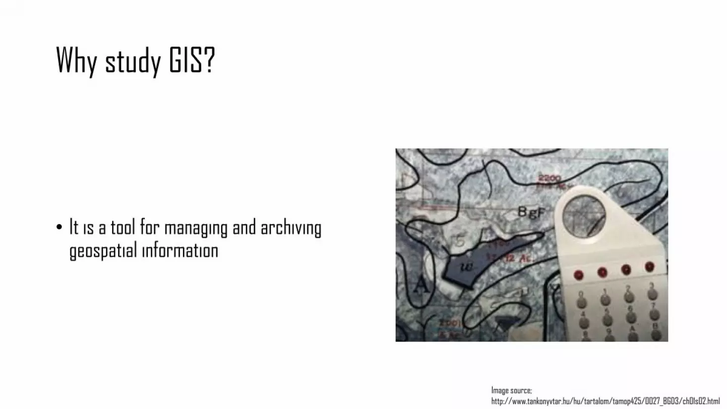
Why study GIS?
• It is a tool for managing and archiving geospatial information
Image source;
http://www.tankonyvtar.hu/hu/tartalom/tamop425/0027_BGD3/ch01s02.html

Why study GIS?
• Et cetera, et cetera…• Bless the digital age
Image source;
http://www.tankonyvtar.hu/hu/tartalom/tamop425/0027_BGD3/ch01s02.html

Applications of GIS
• Urban planning
Image source;
http://www.emba.cat/wp-content/uploads/2013/02/emba_urban-planning-freiham-nord_01F.jpg

Applications of GIS
• Land cover analysis
Image source;
http://prima.pnnl.gov/sites/default/files/LULC.png

Applications of GIS
• Visibility analysis
Image source;
http://www.freegeographytools.com/wp-content/uploads/2011/02/viewshed.jpg

Applications of GIS
• Route analysis
Image source;
http://cyclingquotes.com/news/2015_giro_ditalia_route_analysis/

Applications of GIS
• And many more…
Image source;
http://docs.qgis.org/1.8/en/_images/heatmap_loaded_colour.png

What is QGIS?
• A free and open source GIS
• A volunteer-driven, donor-funded project
• Runs on Linux, Windows, Unix, Mac OSX and Android
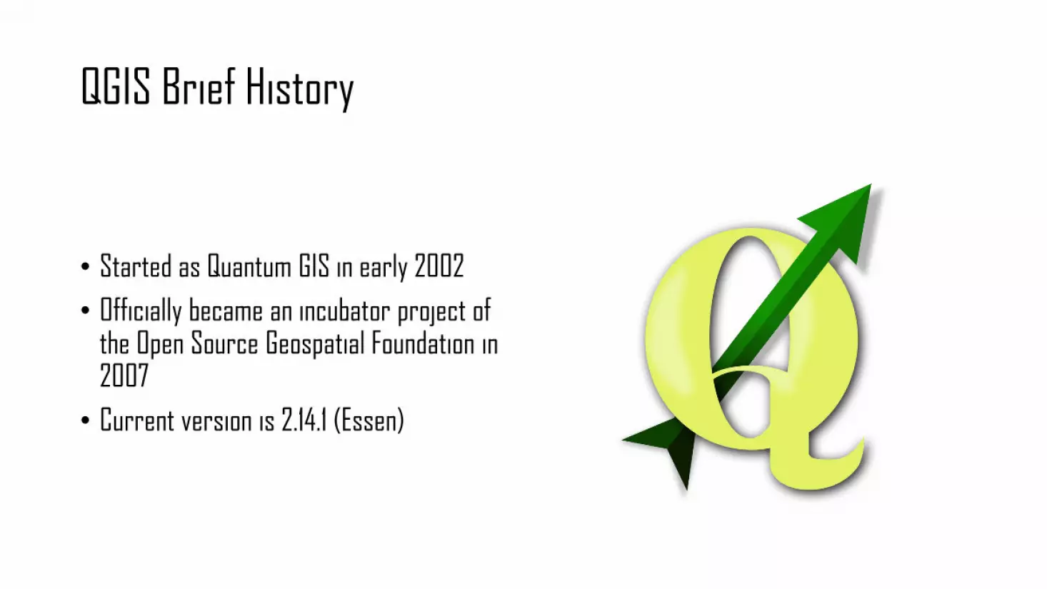
QGIS Brief History
• Started as Quantum GIS in early 2002
• Officially became an incubator project of the Open Source Geospatial Foundation in 2007
• Current version is 2.14.1 (Essen)

When can I NOT use QGIS?
• If you don’t need to use geospatial data in the first place (I was like “duh…”)
• If you already have a licensed ESRI ArcGIS to use• The ArcGIS Toolboxes contain a hefty variety of useful analysis tools
• Some tools in QGIS are not as efficient as their ArcGIS counterparts• i.e. from my previous work experience, the “Dissolve” tool is very much slower in QGIS 1.x (8 hours!!!) than its
ArcGIS counterpart (15 seconds) – though I would have to test it again on QGIS 2.x
• ESRI developed the shapefile data format, and is arguably the one who should understand it best
• ArcGIS is already an industry standard (meaning large corporations and organizations make use of ArcGIS at the production level)

When should I use QGIS?
• If you don’t have an ArcGIS license (QGIS is FREE, ESRI ArcGIS has an expensive license)
• If you need good visualization plugins such as the OpenLayers plugin (ArcGIS doesn’t have an equivalent for it at the moment)
• If you are the adventurous type• a.k.a. you are the type who likes playing around with the growing number of QGIS functionalities –
some of which may not be present in ArcGIS or are better than their ArcGIS counterparts
• If you are into supporting volunteer groups• QGIS developers encourage bug reporting and user experience sharing to greatly improve their
software• Use and promotion of QGIS – and any free and open source software for that matter – can lead into
industry acceptance (think Android!)

Can I use QGIS and ArcGIS simultaneously?
• Of course! No one is stopping you…• Classic case: doing geospatial “homeworks” for your company or organization in your home

A handful of QGIS features and pluginsThat you might like…

Vector digitization
• A must-have for any good GIS application

Raster calculator
• Performs pixel-based mathematical operations
• Useful for processing satellite imagery
1 2 5
2 4 2
7 3 8
3 8 3
5 6 1
8 1 2
+
4 10 8
7 10 3
15 4 10
=

Query builder
• Used in analysis of patterns in vector data

Zonal statistics
• A combined vector-raster toolset
• Used for encapsulating raster values into vector features
• QGIS matches ArcGIS on this one
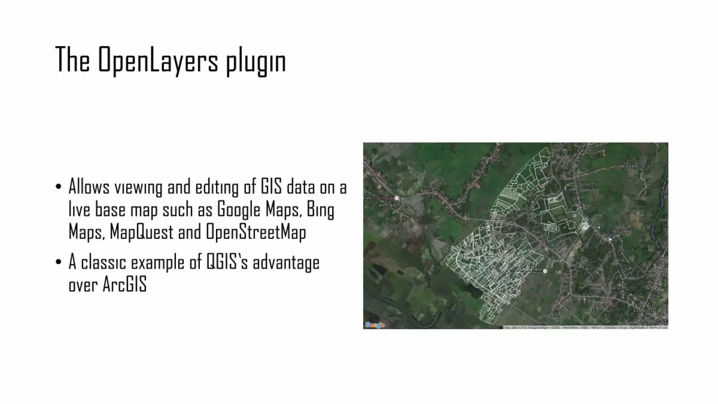
The OpenLayers plugin
• Allows viewing and editing of GIS data on a live base map such as Google Maps, Bing Maps, MapQuest and OpenStreetMap
• A classic example of QGIS’s advantage over ArcGIS
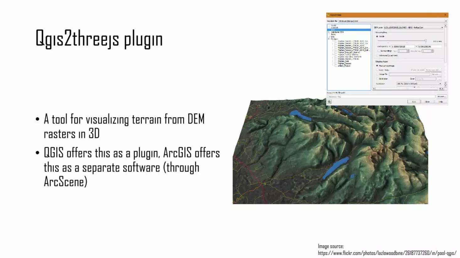
Qgis2threejs plugin
• A tool for visualizing terrain from DEM rasters in 3D
• QGIS offers this as a plugin, ArcGIS offers this as a separate software (through ArcScene)
Image source;
https://www.flickr.com/photos/lazlowoodbine/26187737260/in/pool-qgis/

MMQGIS plugin
• A toolset for combining, loading and saving attribute tables (joining, importing from and exporting to CSV) and other manipulations
• ArcGIS ArcMap already includes the above items within the parenthesis as part of its basic functions, QGIS offers this as a plugin

DB Manager
• A toolset for obtaining and manipulating geospatial information from dedicated geodatabases such as PostGIS, Apache SpatiaLite, MSSQL and Oracle Spatial

Symbology editor
• For styling thematic maps to make them more meaningful to end viewers
• Depends largely on your creativity
• Again, a must-have for any good GIS application

Other QGIS items that can be explored
• Shortest path analysis
• Heatmap generation
• Print composer (I believe the next workshop on QGIS is about this one )
• Others (please specify)

Workshop properBest done hands-on

WARNING!!!
Information overload incoming

Materials Provided
• Three clipped Landsat images of Iligan City and its far peripheries taken at different dates (March 1996, April 2000 and December 1997) projected at UTM Zone 51N
Activity 0: Loading the images
• Step 1: Click on the “K” icon at the leftmost toolbar.
• Step 2: Go to the folder containing the provided materials, select all of the Iligan images and click “Open”.
• Step 3: Check the loaded images (not very pretty, aren’t they?).

Activity 1.1: True color composite
• Step 1: Click on the “Layers Panel” tab at the southwest corner of the interface and uncheck the April 2000 and December 1997 images, leaving the March 1996 image checked.
• Step 2: Right-click on the March 1996 image and select “Properties”.
• Step 3: Go to the “Transparency” section and change the Transparency Band to “None”.
• Step 4: Go to the “Style” section, change the Render Type to “Multiband Color”, change the Red Band to “Band 3”, the Green Band to “Band 2”, the Blue Band to “Band 1”, and the Contrast Enhancement to “Stretch to MinMax”.
• Step 5: Go to the Histogram section and click on the “Calculate Histogram” button if graphs are not displaying (you should see some bell-shaped graphs in the process…)

Activity 1.1: True color composite
(…such as this one)

Activity 1.2: True color composite
• Step 1: Select “Band 1” at the “Set min/max style for” option.
• Step 2: Click on the pointing finger button beside the “Min” entry and try to move the vertical bar as close as possible to the leftmost end of the blue bell curve.
• Step 3: Click on the pointing finger button beside the “Max” entry and try to move the vertical bar as close as possible to the rightmost end of the blue bell curve.
• Step 4: Click on “Apply” and observe the color change on the satellite image.
• Step 5: Repeat the above three steps for “Band 2” and its green curve, and “Band 3” and its red curve, and you should get an image close to a true color image.
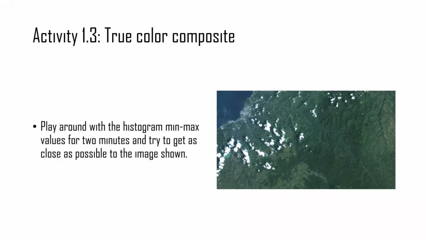
Activity 1.3: True color composite
• Play around with the histogram min-max values for two minutes and try to get as close as possible to the image shown.

Activity 2: False color composite
• Step 1: Go back to the “Style” section, keep the Render Type to “Multiband Color” and the Contrast Enhancement to “Stretch to MinMax”, but this time change the Red Band to “Band 4”, the Green Band to “Band 3” and the Blue Band to “Band 2”.
• Step 2: Repeat Activities 1.2 and 1.3 for the selected bands (you have five minutes ).
• Step 3: Observe the newly created image. Notice the cyan (or close to cyan) colors that contrast very well against the red and green areas (try playing around more with the histogram to get a combination of reddish, greenish and “cyanish” colors). What do you guys and gals think are these areas?
• Step 4: If you guys and gals like to know some physics behind the images, just ask Else, we’ll proceed to Activity 3.

Activity 2: False color composite

Activity 2: False color composite

Activity 3: Land cover analysis
• Step 1: Back at the Layers Panel, uncheck the March 1996 image and check the April 2000 image.
• Step 2: Repeat the entire Activity 2 (and 1.2 and 1.3) for the April 2000 image (you have five minutes ).
• Step 3: Now try switching between the March 1996 and April 2000 image by checking and unchecking one of the two. Did you see some DRASTIC difference? (clue: it’s not near the Iligan City area)

Activity 4.1: Vector digitization
• Step 1: Go to the “Layer” menu at the topmost area and select “Create Layer > New Shapefile Layer…”
• Step 2: Select “Polygon” as Type, change the coordinate reference system to “EPSG:32651 – WGS84 / UTM Zone 51N” (this option should appear at the dropdown box as the Landsat images are projected in this system, but if it doesn’t, click the button beside its dropdown box to open a new window, type “32651” in the Filter dialog box and select the output at the results area below)
• Step 3: Click on “OK” and save the file in the same directory as the Landsat images (i.e. “kamote.shp”).
• Step 4: Click on the “K” icon to toggle editing mode, then click on the “K” button.
• Step 5: Draw a figure around the DRASTIC change (a rectangle is OK) then right-click.
• Step 6: Give any nonnegative integer as the feature’s “id”.
• Step 7: Click on the “K” button to save the feature, and click on the “K” button to de-toggle editing mode.

Activity 4.2: Vector digitization
• Step 1: Right-click on the shapefile in the Layers Panel and select “Open Attribute Table” to open a windowed table.
• Step 2: Click on the “K” icon to open the Field Calculator.
• Step 3: Make sure an ‘x’ mark is on the Create New Table option, type “Area” in the Output Field Name entry, switch the Output Field Type to “Decimal number (real)”, enter “16” as the Output Field Length and “4” as the Precision.
• Step 4: Double-click on “Geometry” at the center and double-click on the “$area” option, then click “OK”.
• Step 5: Check the table and you should see a new column. What does the value in the column say?

(Optional) Activity 5: The OpenLayers plugin
• NOTE: This activity is for those who both have Internet access and have pre-loaded the OpenLayers plugin
• Step 1: Go to the “Web” menu and select “OpenLayers plugin > Google Maps > Google Hybrid”.
• Step 2: At the Layers Panel, drag the Google Hybrid layer to the bottommost position.
• Step 3: Try comparing the Google Hybrid image with the DRASTIC change.
• Step 4: Try loading other base maps from the OpenLayers plugin.

(Really optional) Activity 6: The December 1997 image
• Apply what you guys and gals have learned in this workshop on the December 1997 image and check out the location of the DRASTIC change.

In summary
• GIS is a good tool for creating, manipulating, viewing, assessing and archiving data
• QGIS is a good FOSS GIS for doing the abovementioned chores
• The activities we had just done are merely the tip of the GIS iceberg

Krita, anyone? Shameless Segway for a Free and Open-Source Digital Arts software (go to krita.org for details)

Krita, anyone? Shameless Segway for a Free and Open-Source Digital Arts software (go to krita.org for details)
Image source:
http://www.blendernation.com/wp-content/uploads/2015/05/Krita.jpg