Embed Size (px)
Citation preview
Aalto University
School of Science and Technology
Faculty of Electronics, Communications and Automation
Department of Signal Processing and Acoustics
Erik Axelson
Analysing the Efficiency of Algorithms for
Compiling Finite-State Morphologies
Master’s Thesis
Espoo, April 1, 2010
Supervisor: Professor Paavo Alku
Instructor: Krister Lindén, PhD
2
AALTO‐YLIOPISTON
TEKNILLINEN KORKEAKOULU
Diplomityön tiivistelmä
Tekijä: Erik Axelson
Työn nimi: Äärellistilaisten morfologioiden käännösalgoritmien tehokkuusanalyysi
Päiväys: 1. huhtikuuta 2010 Sivumäärä: 81 + 8
Tiedekunta: Elektroniikan, tietoliikenteen ja automaation tiedekunta
Professuuri: Akustiikka ja äänenkäsittelytekniikka (S-89)
Valvoja: Professori Paavo Alku
Ohjaaja: Krister Lindén, dosentti
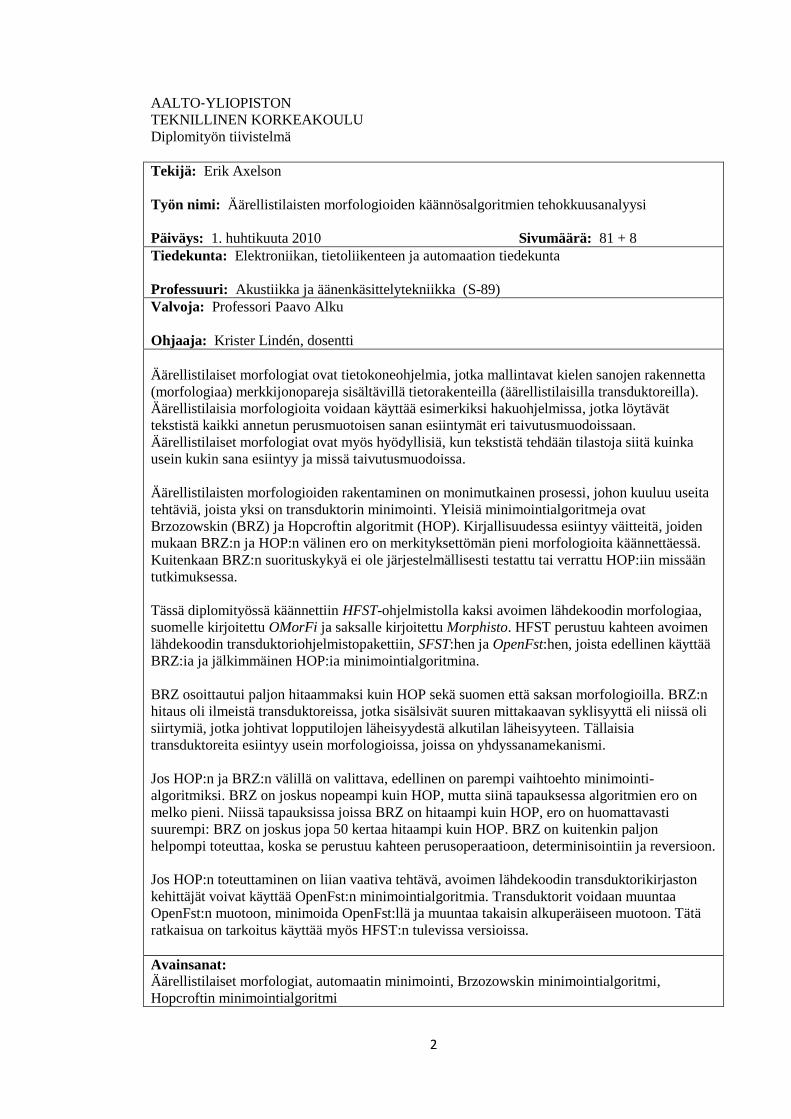
Äärellistilaiset morfologiat ovat tietokoneohjelmia, jotka mallintavat kielen sanojen rakennetta
(morfologiaa) merkkijonopareja sisältävillä tietorakenteilla (äärellistilaisilla transduktoreilla).
Äärellistilaisia morfologioita voidaan käyttää esimerkiksi hakuohjelmissa, jotka löytävät
tekstistä kaikki annetun perusmuotoisen sanan esiintymät eri taivutusmuodoissaan.
Äärellistilaiset morfologiat ovat myös hyödyllisiä, kun tekstistä tehdään tilastoja siitä kuinka
usein kukin sana esiintyy ja missä taivutusmuodoissa.
Äärellistilaisten morfologioiden rakentaminen on monimutkainen prosessi, johon kuuluu useita
tehtäviä, joista yksi on transduktorin minimointi. Yleisiä minimointialgoritmeja ovat
Brzozowskin (BRZ) ja Hopcroftin algoritmit (HOP). Kirjallisuudessa esiintyy väitteitä, joiden
mukaan BRZ:n ja HOP:n välinen ero on merkityksettömän pieni morfologioita käännettäessä.
Kuitenkaan BRZ:n suorituskykyä ei ole järjestelmällisesti testattu tai verrattu HOP:iin missään
tutkimuksessa.
Tässä diplomityössä käännettiin HFST-ohjelmistolla kaksi avoimen lähdekoodin morfologiaa,
suomelle kirjoitettu OMorFi ja saksalle kirjoitettu Morphisto. HFST perustuu kahteen avoimen
lähdekoodin transduktoriohjelmistopakettiin, SFST:hen ja OpenFst:hen, joista edellinen käyttää
BRZ:ia ja jälkimmäinen HOP:ia minimointialgoritmina.
BRZ osoittautui paljon hitaammaksi kuin HOP sekä suomen että saksan morfologioilla. BRZ:n
hitaus oli ilmeistä transduktoreissa, jotka sisälsivät suuren mittakaavan syklisyyttä eli niissä oli
siirtymiä, jotka johtivat lopputilojen läheisyydestä alkutilan läheisyyteen. Tällaisia
transduktoreita esiintyy usein morfologioissa, joissa on yhdyssanamekanismi.
Jos HOP:n ja BRZ:n välillä on valittava, edellinen on parempi vaihtoehto minimointi-
algoritmiksi. BRZ on joskus nopeampi kuin HOP, mutta siinä tapauksessa algoritmien ero on
melko pieni. Niissä tapauksissa joissa BRZ on hitaampi kuin HOP, ero on huomattavasti
suurempi: BRZ on joskus jopa 50 kertaa hitaampi kuin HOP. BRZ on kuitenkin paljon
helpompi toteuttaa, koska se perustuu kahteen perusoperaatioon, determinisointiin ja reversioon.
Jos HOP:n toteuttaminen on liian vaativa tehtävä, avoimen lähdekoodin transduktorikirjaston
kehittäjät voivat käyttää OpenFst:n minimointialgoritmia. Transduktorit voidaan muuntaa
OpenFst:n muotoon, minimoida OpenFst:llä ja muuntaa takaisin alkuperäiseen muotoon. Tätä
ratkaisua on tarkoitus käyttää myös HFST:n tulevissa versioissa.
Avainsanat:
Äärellistilaiset morfologiat, automaatin minimointi, Brzozowskin minimointialgoritmi,
Hopcroftin minimointialgoritmi
3
AALTO UNIVERSITY
SCHOOL OF SCIENCE AND TECHNOLOGY
Abstract of the Master’s thesis
Author: Erik Axelson
Name of the thesis:
Analysing the Efficiency of Algorithms for Compiling Finite-State Morphologies
Date: April 1, 2010 Number of pages: 81 + 8
Faculty: Faculty of Electronics, Communications and Automation
Professorship: Acoustics and Audio Signal Processing (S-89)
Supervisor: Professor Paavo Alku
Instructor: Krister Lindén, PhD
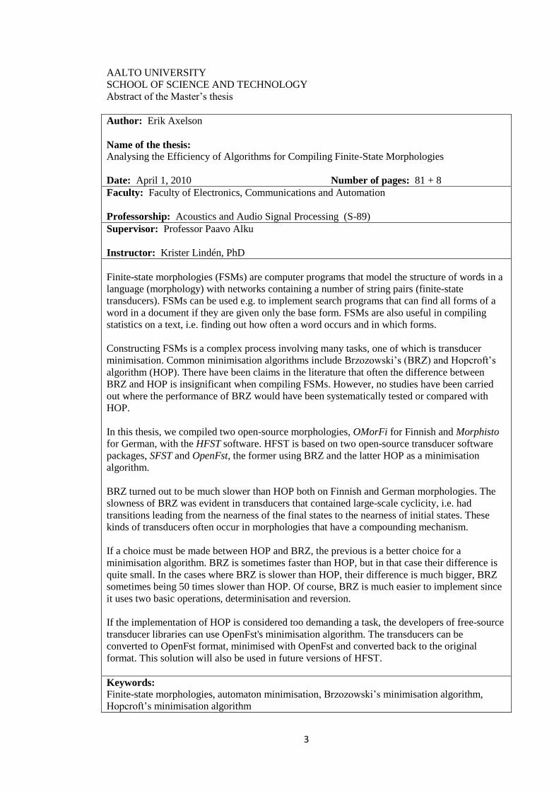
Finite-state morphologies (FSMs) are computer programs that model the structure of words in a
language (morphology) with networks containing a number of string pairs (finite-state
transducers). FSMs can be used e.g. to implement search programs that can find all forms of a
word in a document if they are given only the base form. FSMs are also useful in compiling
statistics on a text, i.e. finding out how often a word occurs and in which forms.
Constructing FSMs is a complex process involving many tasks, one of which is transducer
minimisation. Common minimisation algorithms include Brzozowski’s (BRZ) and Hopcroft’s
algorithm (HOP). There have been claims in the literature that often the difference between
BRZ and HOP is insignificant when compiling FSMs. However, no studies have been carried
out where the performance of BRZ would have been systematically tested or compared with
HOP.
In this thesis, we compiled two open-source morphologies, OMorFi for Finnish and Morphisto
for German, with the HFST software. HFST is based on two open-source transducer software
packages, SFST and OpenFst, the former using BRZ and the latter HOP as a minimisation
algorithm.
BRZ turned out to be much slower than HOP both on Finnish and German morphologies. The
slowness of BRZ was evident in transducers that contained large-scale cyclicity, i.e. had
transitions leading from the nearness of the final states to the nearness of initial states. These
kinds of transducers often occur in morphologies that have a compounding mechanism.
If a choice must be made between HOP and BRZ, the previous is a better choice for a
minimisation algorithm. BRZ is sometimes faster than HOP, but in that case their difference is
quite small. In the cases where BRZ is slower than HOP, their difference is much bigger, BRZ
sometimes being 50 times slower than HOP. Of course, BRZ is much easier to implement since
it uses two basic operations, determinisation and reversion.
If the implementation of HOP is considered too demanding a task, the developers of free-source
transducer libraries can use OpenFst's minimisation algorithm. The transducers can be
converted to OpenFst format, minimised with OpenFst and converted back to the original
format. This solution will also be used in future versions of HFST.
Keywords:
Finite-state morphologies, automaton minimisation, Brzozowski’s minimisation algorithm,
Hopcroft’s minimisation algorithm

4
Preface
This thesis has been written at the Department of General Linguistics at the University
of Helsinki as a part of the Helsinki Finite-State Transducer Technology (HFST)
project.
My gratitude goes to my instructor Dr. Krister Lindén for support and valuable
comments. I also thank all members of the HFST project for giving me advice and
sharing their expertise throughout the work progress. I thank my supervisor Professor
Paavo Alku for reading and commenting on my thesis. I am very grateful for my
mother, friends and relatives for support during my studies and work.
Helsinki, Finland
April 12, 2010
Erik Axelson
5
Table of contents
Diplomityön tiivistelmä ............................................................................................................. 2
Abstract of the Master’s thesis ................................................................................................. 3
Preface ...................................................................................................................................... 4
Table of contents ...................................................................................................................... 5
Abbreviations and acronyms .................................................................................................... 7
Notations................................................................................................................................... 8
Symbols ..................................................................................................................................... 9
1. Introduction ........................................................................................................................ 10
1.1 A short introduction to finite-state morphologies ........................................................ 10
1.2 The thesis ...................................................................................................................... 11
2. Background in Linguistics .................................................................................................... 15
2.1 Definitions of Linguistic Terms ...................................................................................... 15
2.2 Morphology ................................................................................................................... 17
3. Background in Computing Science ...................................................................................... 23
3.1 Finite-State Automata ................................................................................................... 23
3.2 Finite-State Transducers ............................................................................................... 24
3.3 FSTs and regular expressions ........................................................................................ 26
3.4 Transducer operations and properties ......................................................................... 32
4. Finite-State Morphologies (FSMs) ...................................................................................... 36
4.1 What are FSMs? ............................................................................................................ 36
4.2 Where can FSMs be used? ............................................................................................ 37
4.3 Guessing unknown words ............................................................................................. 38
4.4 Compiling FSMs ............................................................................................................. 39
4.5 FSM rules ....................................................................................................................... 42
5. Minimisation ....................................................................................................................... 46
5.1 Memory consumption................................................................................................... 46
5.2 Time consumption ........................................................................................................ 47
5.3 Minimisation algorithms ............................................................................................... 49
6. Data ..................................................................................................................................... 60
6.1 SFST programming language (SFST-PL) ......................................................................... 60
6.2 OMorFi .......................................................................................................................... 62
6
6.3 Morphisto...................................................................................................................... 63
7. Tests .................................................................................................................................... 65
7.1 The tools and strategy................................................................................................... 65
7.2 Are there differences? .................................................................................................. 67
7.3 What explains the differences? .................................................................................... 69
7.4 Comparing the minimisation algorithms ...................................................................... 72
7.5 What explains the differences in HOP and BRZ? .......................................................... 74
7.6 What happens in minimisation? ................................................................................... 75
7.7 Testing the cyclicity hypothesis .................................................................................... 77
8. Discussion ............................................................................................................................ 83
8.1 The results from the tests summarised ........................................................................ 83
8.2 Comparisons with literature ......................................................................................... 84
8.3 Future work ................................................................................................................... 84
9. Conclusions ......................................................................................................................... 87
List of references ..................................................................................................................... 89
7
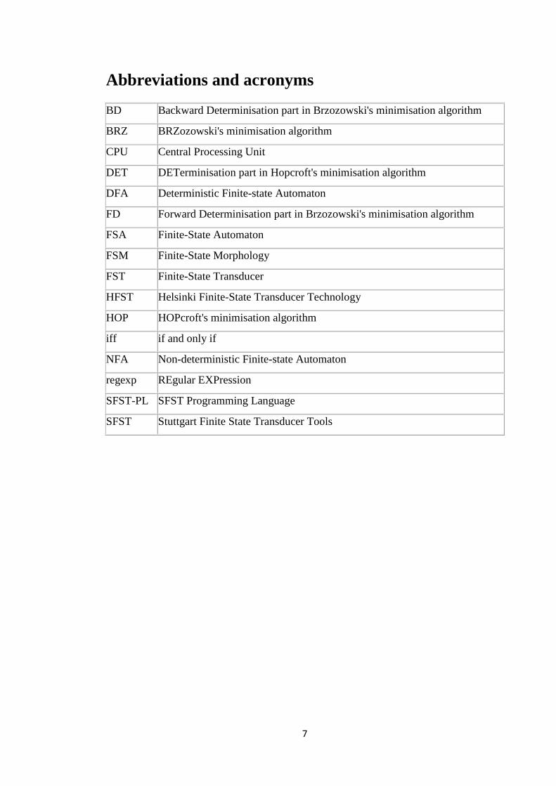
Abbreviations and acronyms
BD Backward Determinisation part in Brzozowski's minimisation algorithm
BRZ BRZozowski's minimisation algorithm
CPU Central Processing Unit
DET DETerminisation part in Hopcroft's minimisation algorithm
DFA Deterministic Finite-state Automaton
FD Forward Determinisation part in Brzozowski's minimisation algorithm
FSA Finite-State Automaton
FSM Finite-State Morphology
FST Finite-State Transducer
HFST Helsinki Finite-State Transducer Technology
HOP HOPcroft's minimisation algorithm
iff if and only if
NFA Non-deterministic Finite-state Automaton
regexp REgular EXPression
SFST-PL SFST Programming Language
SFST Stuttgart Finite State Transducer Tools
8
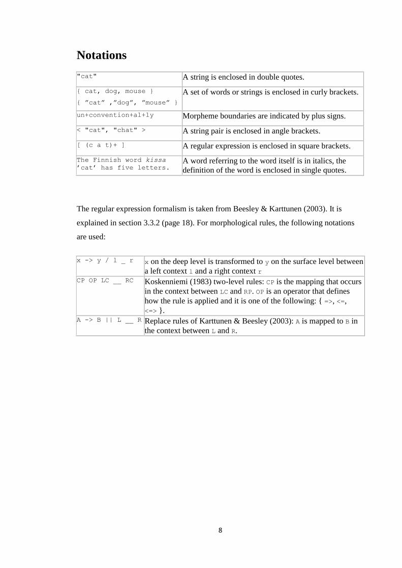
Notations
"cat" A string is enclosed in double quotes.
{ cat, dog, mouse }
{ ”cat” ,”dog”, ”mouse” }
A set of words or strings is enclosed in curly brackets.
un+convention+al+ly Morpheme boundaries are indicated by plus signs.
< "cat", "chat" > A string pair is enclosed in angle brackets.
[ (c a t)+ ] A regular expression is enclosed in square brackets.
The Finnish word kissa
’cat’ has five letters. A word referring to the word itself is in italics, the
definition of the word is enclosed in single quotes.
The regular expression formalism is taken from Beesley & Karttunen (2003). It is
explained in section 3.3.2 (page 18). For morphological rules, the following notations
are used:
x -> y / l _ r x on the deep level is transformed to y on the surface level between
a left context l and a right context r CP OP LC __ RC Koskenniemi (1983) two-level rules: CP is the mapping that occurs
in the context between LC and RP. OP is an operator that defines
how the rule is applied and it is one of the following: { =>, <=,
<=> }. A -> B || L __ R Replace rules of Karttunen & Beesley (2003): A is mapped to B in
the context between L and R.
9
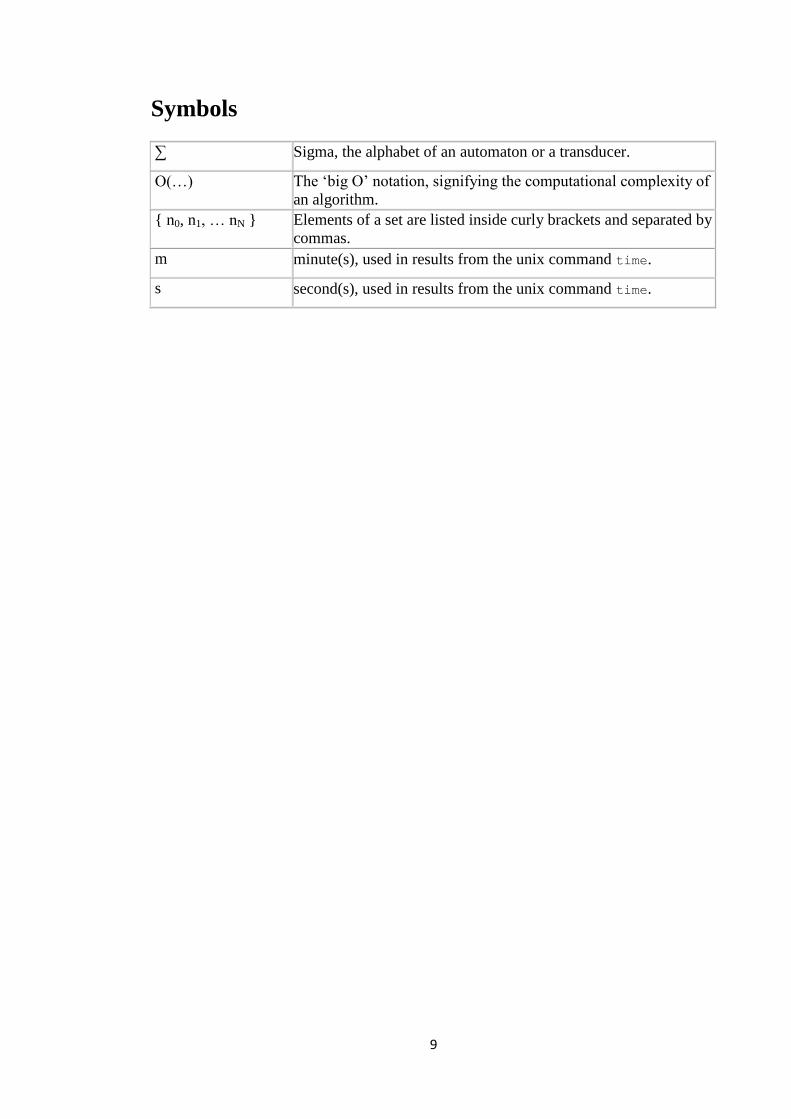
Symbols
∑ Sigma, the alphabet of an automaton or a transducer.
O(…) The ‘big O’ notation, signifying the computational complexity of
an algorithm.
{ n0, n1, … nN } Elements of a set are listed inside curly brackets and separated by
commas.
m minute(s), used in results from the unix command time.
s second(s), used in results from the unix command time.
10
1. Introduction
This chapter contains a very short introduction to finite-state morphologies and some
information on the purpose and structure of this thesis.
For an extended introduction on finite-state morphologies, see Beesley & Karttunen
(2003) and Karlsson (2004).
1.1 A short introduction to finite-state morphologies
Finite-state morphology (FSM) is a field of computational linguistics that studies how
finite-state transducers (FSTs) can be used to model the morphology of a language.
FSTs are networks that recognise a set of strings and for each recognised input string,
produce one or more corresponding output strings. Morphology is a field of linguistics
that studies the structure of words, i.e. how words are formed from smaller units and, on
the other hand, how these units can be combined into words.
By combining linguistic knowledge of the morphology of a language and FSTs, it is
possible to create computer programs that model the structure of words in the language.
The term FSM is also used to refer to these programs.
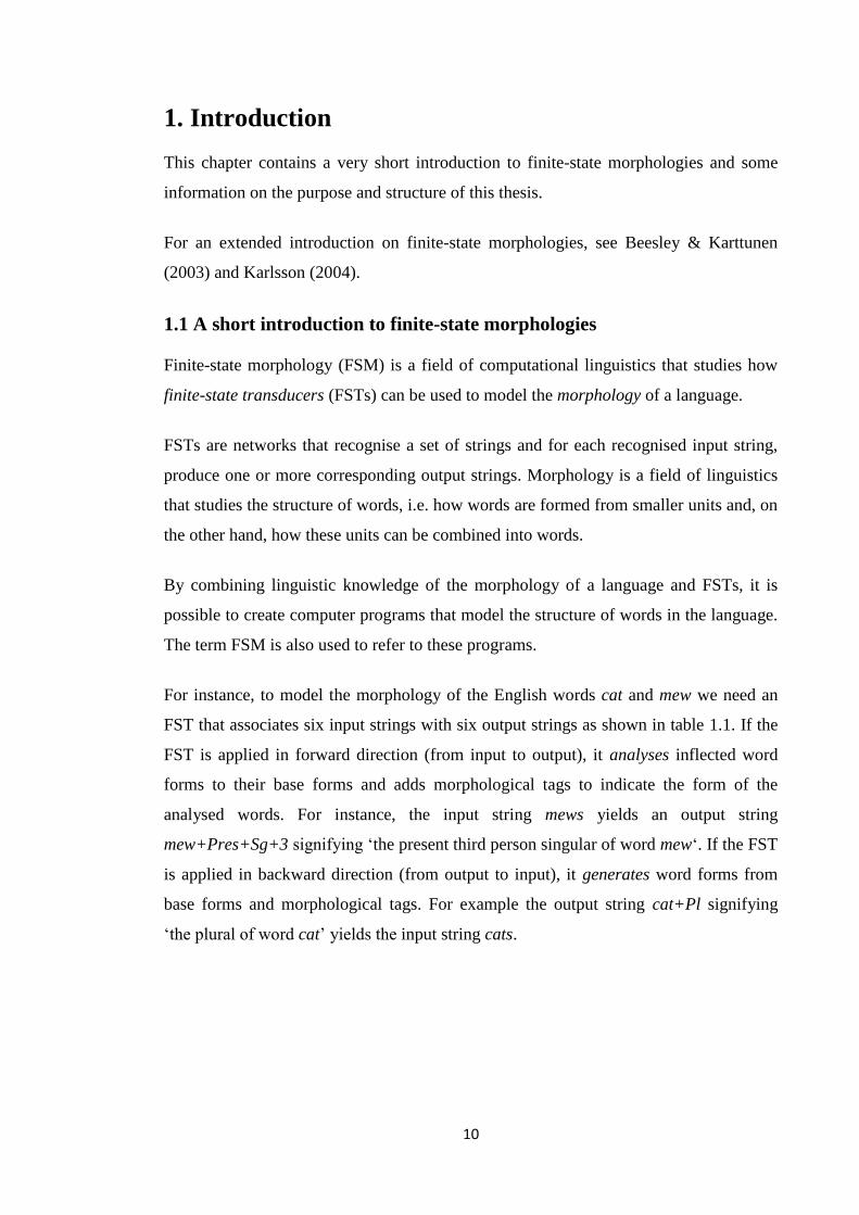
For instance, to model the morphology of the English words cat and mew we need an
FST that associates six input strings with six output strings as shown in table 1.1. If the
FST is applied in forward direction (from input to output), it analyses inflected word
forms to their base forms and adds morphological tags to indicate the form of the
analysed words. For instance, the input string mews yields an output string
mew+Pres+Sg+3 signifying ‘the present third person singular of word mew‘. If the FST
is applied in backward direction (from output to input), it generates word forms from
base forms and morphological tags. For example the output string cat+Pl signifying
‘the plural of word cat’ yields the input string cats.
11
Table 1.1: An FST that associates inflected word forms with their analyses.
input string output string
cat cat+Sg
cats cat+Pl
mew mew+Pres
mews mew+Pres+Sg+3
mewed mew+Past
mewing mew+Inf
This kind of FSMs are very effective. Both analysis and generation mode can be useful
if we want to find all forms of a word in a document by giving only the base form to a
search program. The analysis mode is useful if we want to compile statistics on a text,
e.g. find out how often a word occurs and in which forms. It can also be helpful for a
language learner encountering an unfamiliar word in inflected form in a text.
The way FSMs are applied effectively to analyse or generate strings is an important
field of study. However, in this thesis we are going to concentrate on the creation (or
compiling) of FSMs. Compiling finite-state morphologies is a complex process
involving many tasks. One of these tasks is FST minimisation that is often performed a
number of times during FSM compilation.
1.2 The thesis
1.2.1 Background
This thesis has been written at the Department of General Linguistics at the University
of Helsinki as a part of the Helsinki Finite-State Transducer Technology (HFST)
project. The HFST software is intended for the implementation of morphological
analysers and other tools which are based on weighted and unweighted finite-state
transducer technology. The work is licensed under a GNU Lesser General Public
License version 3.0. The HFST functionalities have two main implementations, an
unweighted and a weighted one. The implementations are based on two open-source
12
transducer software packages, SFST - Stuttgart Finite State Transducer Tools and
OpenFst.
1.2.2 The purpose of the thesis
The purpose of the thesis is to compare the two underlying transducer software
packages, SFST and OpenFst, by compiling two open-source morphologies, OMorFi
and Morphisto. OMorFi is a computational morphology for Finnish and Morphisto for
German. The hypothesis is that the pieces of software differ on the algorithmic level
which shows in the compilation times of the FSMs. Questions are: Which functions are
faster in one or the other piece of software? What differences are there on the
algorithmic level that explain the difference? Does the language of the FSM affect
performance?
A preliminary hypothesis is that minimisation is faster in either software package
because their minimisation algorithms differ, SFST using Brzozowski's and OpenFst
Hopcroft's algorithm. However, it is not clear how much this difference affects the
overall performance. There have been claims in the literature (see section 5.3.4 for
references) that often the difference is insignificant when compiling morphologies, but
this does not correspond to our performance observations.
1.2.3 Previous studies
There are many minimisation algorithms available. HOP is theoretically the fastest but
BRZ is often stated to perform as well as HOP in practise despite its theoretically lower
performance. However, no studies have been carried out where the performance of BRZ
would have been systematically tested or compared with HOP. This thesis intends to fill
this gap in BRZ benchmarking. More information on minimisation algorithms and
references to previous studies can be found in chapter 5.
1.2.4 The structure of the thesis
This thesis is divided into eight chapters. The first three chapters contain the
background information that is needed to understand this thesis. The fourth chapter
discusses different minimisation methods. The fifth chapter presents the data used and
the sixth one describes the tests performed. The two last chapters contain discussion on
the results and conclusions.
13
The first chapter presents background information on linguistics. Some general
linguistic terms are defined and the reader is introduced to the field of morphology. The
concepts of the two-level formalism and rules are illustrated with examples.
The second chapter contains background information on computing science. Finite-state
automata and transducers are presented with simple examples. Regular expression
operators and their notations are defined. Regexps and FSTs are identified as a way to
define regular languages and the concept of regular languages is defined. The properties
of transducers and their determinisation and minimisation are briefly discussed. An
example of how regular expressions can be compiled into FSTs is also given.
The third chapter is about finite-state morphologies. Topics that are considered include:
what are FSMs, how and where can they be used, how should unknown words be
handled, how are FSMs compiled and what kind of software is needed in the
compilation. Common linguistic phenomena and the way they should be taken into
consideration are also discussed. Different kinds of FSM rules are presented through
examples.
The fourth chapter discusses the process of FST minimisation and its effect on
performance. Both time end memory issues are covered. Common minimisation
algorithms are presented and their theoretical performances are compared. Previous
papers on FST minimisation are also reviewed.
The fifth chapter presents the data that is used in the tests. Two finite-state
morphologies, OMorFi and Morphisto are presented as well as the SFST programming
language that they are written with.
The sixth chapter describes the tests. The software used in compiling the test data as
well as the profiling programs are briefly presented. Some technical specifications are
also given. A benchmarking strategy to be used in the testing part is outlined. When the
tests are performed, it turns out that there are differences in performance and that they
are due to different minimisation algorithms. The minimisation algorithms are
compared and the results are illustrated in figures. Some analyses are also provided in
order for the interested reader to be able to perform additional tests.

14
In the seventh chapter, results from the tests are summarised and compared with the
results from other studies. Further work is also outlined.
The eighth chapter contains conclusions drawn from the tests.
15
2. Background in Linguistics
This chapter presents background information on linguistics. Some general linguistic
terms are defined and the field of morphology is touched. The concepts of the two-level
formalism and rules are illustrated with examples.
For more information on linguistics and morphology see Karlsson (2004) and on two-
level formalism Koskenniemi (1983).
2.1 Definitions of Linguistic Terms
2.1.1 Lexemes, word forms and words
Usually two or three senses of the term word are distinguished in linguistics (Karlsson,
2004; section 4.1.2). If it is clear from the context what sense is intended or we speak on
a general level, the term word is often enough. However, sometimes we want to make a
distinction among lexemes, word forms and words. To clarify these concepts, we use the
following example text:
There is a cat in the street. There are cats in the streets.
Word is a general term that sometimes has a more specific meaning 'an occurrence of a
word' as opposed to a lexeme or a word form. The example text contains 13 words or
occurrences of a word: there, is a, cat, on, the street, there, are, cats, in, the, streets.
A word form means a word in a certain inflected form. Several instances of the same
word form are counted as one. The example text thus contains 10 word forms: there, is,
a, cat, in, the, street, are, cats, streets.
A lexeme is an abstract concept that refers to all word forms that are related to each
other through inflection (Karlsson, 2004; section 6.1). A lexeme is realised in text or
speech as word forms. A certain word form is usually chosen to represent a lexeme and
it is called a lemma, or citation form or base form. Usually it is the least marked and
simplest form, i.e. in the case of nouns the singular nominative and in the case of verbs
the active present infinitive. The example text has 7 lexemes: there, be, a, cat, in, the,
street. Here be, cat and street are lemmas that represent the lexemes that are realised as
word forms is, are, cat, cats, street, streets.
16
2.1.2 Inflection, derivation and compounding
In the previous section, a lexeme was defined as an abstract concept for all word forms
that are related to each other through inflection. The distinction between inflection and
derivation is not always clear, but the following rules are usually sufficient (Karlsson,
2006; sections 4.5 and 6.4):
1) In inflection, some aspect of a word is changed, but not the meaning or word class.
Aspects that might change include number, tense and mood. For instance cat and cats
belong to the same lexeme because only their numbers differ. Similarly, bake in the
sentence I bake, bakes in He bakes, baked in She would have baked and baking in They
are baking are inflected forms of the same lexeme as they all refer to the same meaning,
only their tenses and moods are different. On the contrary, bake and baker are different
lexemes, baker being a word derived from bake. Here the word class and meaning are
both changed. Baker is a noun referring to a person baking, bake a verb meaning the act
of baking.
2) Inflection follows a paradigm that can be applied to every word in the same word
class. For example, the singular third person in verbs is clearly an inflectional paradigm
as it exists for every verb: bake - bakes, make - makes, be - is, etc. As an opposite
example, the paradigm bake - bakery does not belong to the domain of inflection but
derivation. There exist only few words to which this paradigm can be applied. With
most verbs it does not produce meaningful words, e.g. make - makery and be - beery are
clearly ungrammatical.
New lexemes can be derived from existing ones also through compounding.
Compounds can be written as one word (bedroom), as separate words (high school) or
with hyphens (mother-in-law). Sometimes there must be an additional infix between the
individual words, e.g. German Arbeit 'work' and Zimmer 'room' form a compound
Arbeit+s+zimmer 'work room' as opposed to Schlaf 'dream' and Zimmer that form their
compound without an infix: Schlaf+zimmer 'bedroom'. Most Swedish two-part
compounds do not need an infix: peppar+kaka ('gingerbread', literarily 'pepper biscuit')
and kak+burk ('biscuit jar') are formed by just connecting two words together. However,
in three-part compounds this approach is not enough: peppar+kak+burk is
ungrammatical, only peppar+kak+s+burk ('gingerbread jar', literarily 'pepper biscuit
17
jar') is correct. This is because there must be an infix s between the second and third
morpheme in three-part compounds. Some Swedish two-part compounds also introduce
phonological variation: kyrka, 'church' and gård , 'yard' form a compound kyrko+gård,
'churchyard' and gata, 'street' and bild, 'view' a compound gatu+bild, 'street view'.
2.2 Morphology
2.2.1 Morphemes and morphs
Morphology is a field of linguistics that studies the structure of words. It describes how
words are formed from smaller units called morphemes. A morpheme is defined as the
minimal meaningful unit of a language (Karlsson, 2006; section 4). Morphemes can be
free or bound (Ibid; 4.4). A free morpheme can constitute a word on its own but a bound
morpheme must be appended to a free morpheme, called a root morpheme.
For example the English word unconventionally can be divided into its morphemes in
the following way: un+convention+al+ly (morphemes are separated by a plus sign).
Here convention is a root morpheme to which three bound morphemes are appended.
The meaning of each morpheme can be illustrated by first taking the root morpheme and
then appending the bound morphemes to it one by one. The free morpheme convention
as such means 'custom, practice'. The bound morpheme al expresses quality,
convention+al thus means 'adhering to customs and practices'. The bound morpheme un
expresses negation, so un+convention+al has the meaning 'not adhering to customs and
practices'. The bound morpheme ly expresses the way something is done, so the
meaning of un+convention+al+ly is 'in a fashion of not adhering to customs and
practices'.
Compound words have several free morphemes. Usually the compound is considered as
a single root where bound morphemes are added: bedroom+s, aircondition+ed, extra-
+hardworking, but sometimes one of the free morphs acts as a root: mother+s-in-law,
passer+s-by.
Actually, in the examples above, we did not divide words into their morphemes but
morphs. A morpheme is an abstract concept that is realised as morphs (Ibid; 4.2). For
example in the word cats the plural is indicated by the morph s but in the word oxen by
the morph en and in the plural word sheep as an empty morph. Other noun plural
18
morphs include a as in automaton - automata, i as in cactus - cacti etc. All morphs still
have an identical meaning, so they represent the same morpheme. The morpheme
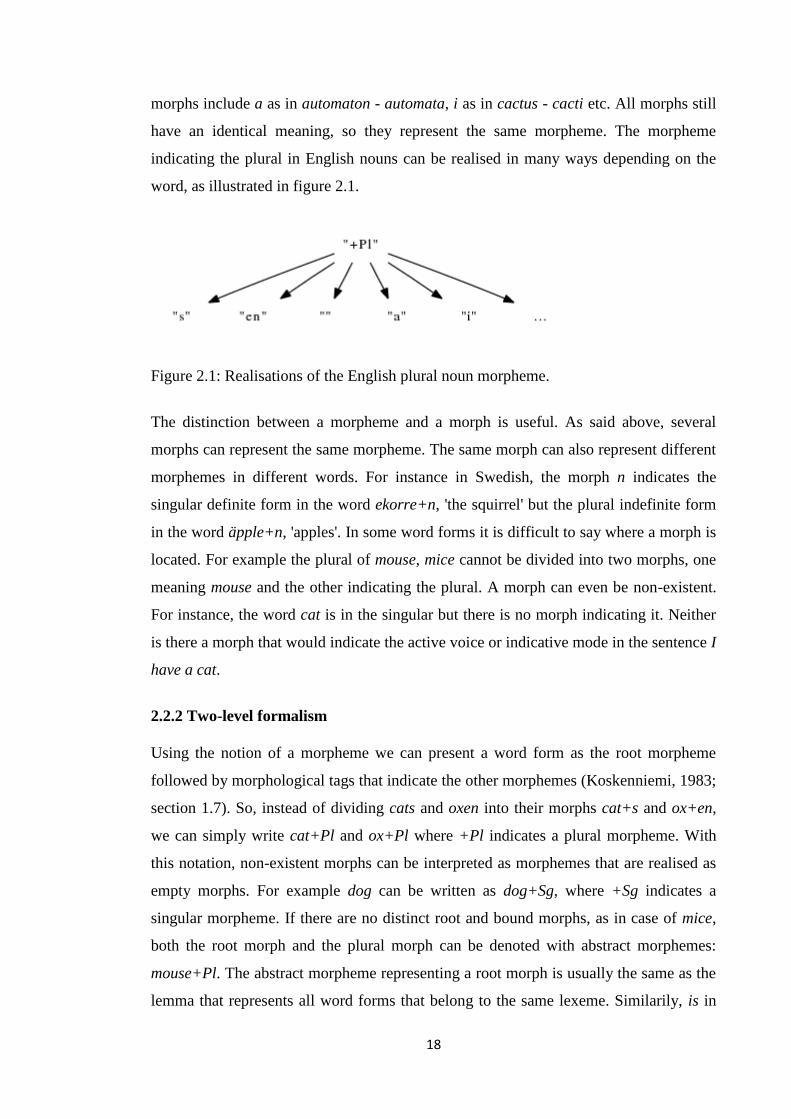
indicating the plural in English nouns can be realised in many ways depending on the
word, as illustrated in figure 2.1.
Figure 2.1: Realisations of the English plural noun morpheme.
The distinction between a morpheme and a morph is useful. As said above, several
morphs can represent the same morpheme. The same morph can also represent different
morphemes in different words. For instance in Swedish, the morph n indicates the
singular definite form in the word ekorre+n, 'the squirrel' but the plural indefinite form
in the word äpple+n, 'apples'. In some word forms it is difficult to say where a morph is
located. For example the plural of mouse, mice cannot be divided into two morphs, one
meaning mouse and the other indicating the plural. A morph can even be non-existent.
For instance, the word cat is in the singular but there is no morph indicating it. Neither
is there a morph that would indicate the active voice or indicative mode in the sentence I
have a cat.
2.2.2 Two-level formalism
Using the notion of a morpheme we can present a word form as the root morpheme
followed by morphological tags that indicate the other morphemes (Koskenniemi, 1983;
section 1.7). So, instead of dividing cats and oxen into their morphs cat+s and ox+en,
we can simply write cat+Pl and ox+Pl where +Pl indicates a plural morpheme. With
this notation, non-existent morphs can be interpreted as morphemes that are realised as
empty morphs. For example dog can be written as dog+Sg, where +Sg indicates a
singular morpheme. If there are no distinct root and bound morphs, as in case of mice,
both the root morph and the plural morph can be denoted with abstract morphemes:
mouse+Pl. The abstract morpheme representing a root morph is usually the same as the
lemma that represents all word forms that belong to the same lexeme. Similarily, is in
19
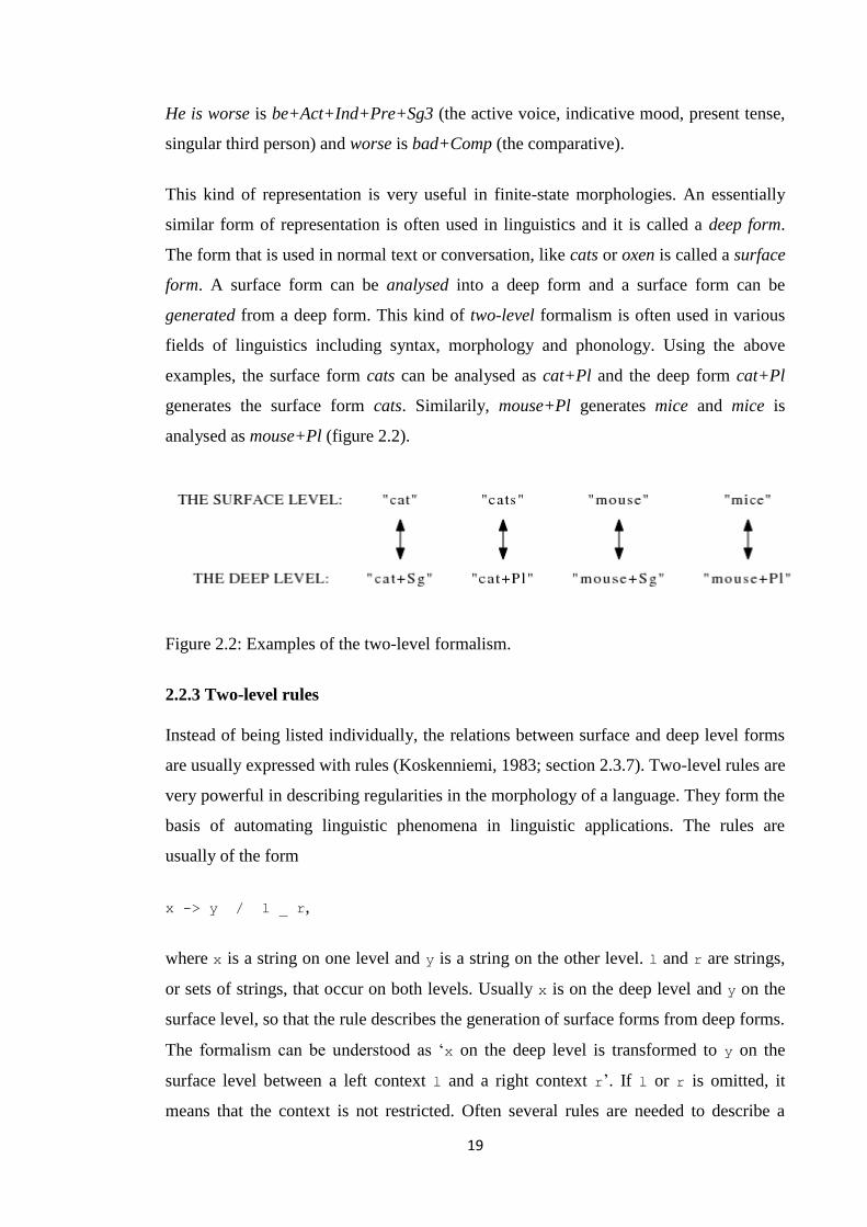
He is worse is be+Act+Ind+Pre+Sg3 (the active voice, indicative mood, present tense,
singular third person) and worse is bad+Comp (the comparative).
This kind of representation is very useful in finite-state morphologies. An essentially
similar form of representation is often used in linguistics and it is called a deep form.
The form that is used in normal text or conversation, like cats or oxen is called a surface
form. A surface form can be analysed into a deep form and a surface form can be
generated from a deep form. This kind of two-level formalism is often used in various
fields of linguistics including syntax, morphology and phonology. Using the above
examples, the surface form cats can be analysed as cat+Pl and the deep form cat+Pl
generates the surface form cats. Similarily, mouse+Pl generates mice and mice is
analysed as mouse+Pl (figure 2.2).
Figure 2.2: Examples of the two-level formalism.
2.2.3 Two-level rules
Instead of being listed individually, the relations between surface and deep level forms
are usually expressed with rules (Koskenniemi, 1983; section 2.3.7). Two-level rules are
very powerful in describing regularities in the morphology of a language. They form the
basis of automating linguistic phenomena in linguistic applications. The rules are
usually of the form
x -> y / l _ r,
where x is a string on one level and y is a string on the other level. l and r are strings,
or sets of strings, that occur on both levels. Usually x is on the deep level and y on the
surface level, so that the rule describes the generation of surface forms from deep forms.
The formalism can be understood as ‘x on the deep level is transformed to y on the
surface level between a left context l and a right context r’. If l or r is omitted, it
means that the context is not restricted. Often several rules are needed to describe a
20
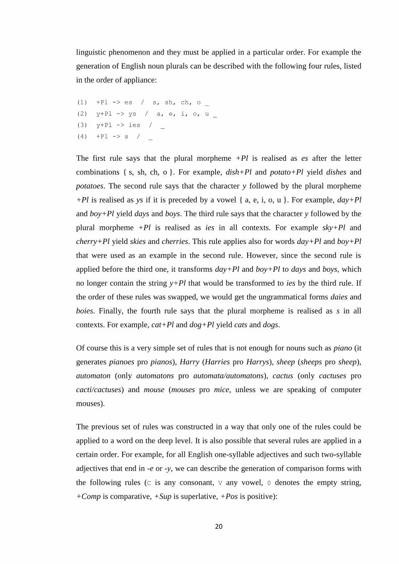
linguistic phenomenon and they must be applied in a particular order. For example the
generation of English noun plurals can be described with the following four rules, listed
in the order of appliance:
(1) +Pl -> es / s, sh, ch, o _
(2) y+Pl -> ys / a, e, i, o, u _
(3) y+Pl -> ies / _
(4) +Pl -> s / _
The first rule says that the plural morpheme +Pl is realised as es after the letter
combinations { s, sh, ch, o }. For example, dish+Pl and potato+Pl yield dishes and
potatoes. The second rule says that the character y followed by the plural morpheme
+Pl is realised as ys if it is preceded by a vowel { a, e, i, o, u }. For example, day+Pl
and boy+Pl yield days and boys. The third rule says that the character y followed by the
plural morpheme +Pl is realised as ies in all contexts. For example sky+Pl and
cherry+Pl yield skies and cherries. This rule applies also for words day+Pl and boy+Pl
that were used as an example in the second rule. However, since the second rule is
applied before the third one, it transforms day+Pl and boy+Pl to days and boys, which
no longer contain the string y+Pl that would be transformed to ies by the third rule. If
the order of these rules was swapped, we would get the ungrammatical forms daies and
boies. Finally, the fourth rule says that the plural morpheme is realised as s in all
contexts. For example, cat+Pl and dog+Pl yield cats and dogs.
Of course this is a very simple set of rules that is not enough for nouns such as piano (it
generates pianoes pro pianos), Harry (Harries pro Harrys), sheep (sheeps pro sheep),
automaton (only automatons pro automata/automatons), cactus (only cactuses pro
cacti/cactuses) and mouse (mouses pro mice, unless we are speaking of computer
mouses).
The previous set of rules was constructed in a way that only one of the rules could be
applied to a word on the deep level. It is also possible that several rules are applied in a
certain order. For example, for all English one-syllable adjectives and such two-syllable
adjectives that end in -e or -y, we can describe the generation of comparison forms with
the following rules (C is any consonant, V any vowel, 0 denotes the empty string,
+Comp is comparative, +Sup is superlative, +Pos is positive):
21
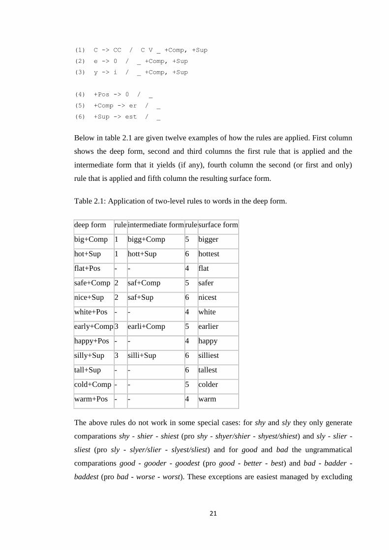
(1) C -> CC / C V _ +Comp, +Sup
(2) e -> 0 / _ +Comp, +Sup
(3) y -> i / _ +Comp, +Sup
(4) +Pos -> 0 / _
(5) +Comp -> er / _
(6) +Sup -> est / _
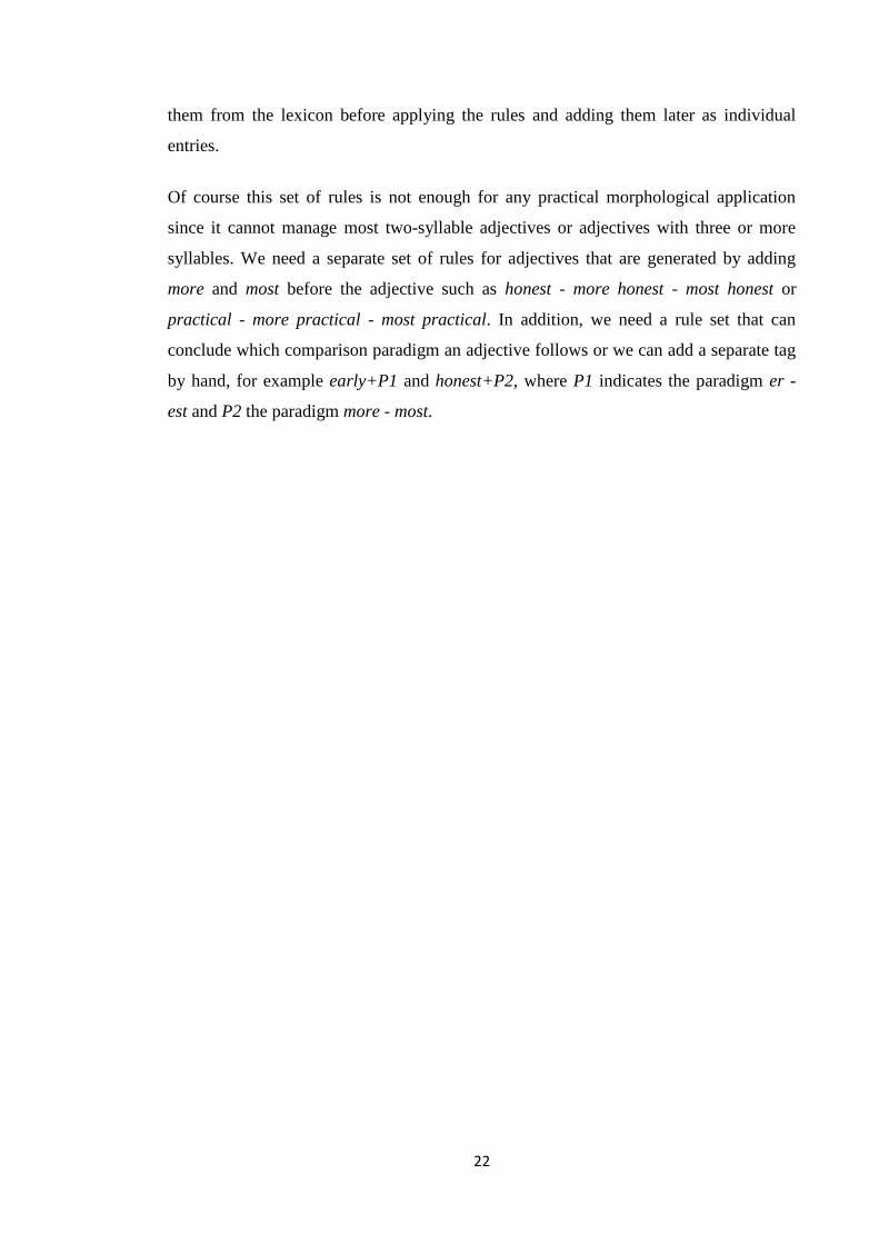
Below in table 2.1 are given twelve examples of how the rules are applied. First column
shows the deep form, second and third columns the first rule that is applied and the
intermediate form that it yields (if any), fourth column the second (or first and only)
rule that is applied and fifth column the resulting surface form.
Table 2.1: Application of two-level rules to words in the deep form.
deep form rule intermediate form rule surface form
big+Comp 1 bigg+Comp 5 bigger
hot+Sup 1 hott+Sup 6 hottest
flat+Pos - - 4 flat
safe+Comp 2 saf+Comp 5 safer
nice+Sup 2 saf+Sup 6 nicest
white+Pos - - 4 white
early+Comp 3 earli+Comp 5 earlier
happy+Pos - - 4 happy
silly+Sup 3 silli+Sup 6 silliest
tall+Sup - - 6 tallest
cold+Comp - - 5 colder
warm+Pos - - 4 warm
The above rules do not work in some special cases: for shy and sly they only generate
comparations shy - shier - shiest (pro shy - shyer/shier - shyest/shiest) and sly - slier -
sliest (pro sly - slyer/slier - slyest/sliest) and for good and bad the ungrammatical
comparations good - gooder - goodest (pro good - better - best) and bad - badder -
baddest (pro bad - worse - worst). These exceptions are easiest managed by excluding
22
them from the lexicon before applying the rules and adding them later as individual
entries.
Of course this set of rules is not enough for any practical morphological application
since it cannot manage most two-syllable adjectives or adjectives with three or more
syllables. We need a separate set of rules for adjectives that are generated by adding
more and most before the adjective such as honest - more honest - most honest or
practical - more practical - most practical. In addition, we need a rule set that can
conclude which comparison paradigm an adjective follows or we can add a separate tag
by hand, for example early+P1 and honest+P2, where P1 indicates the paradigm er -
est and P2 the paradigm more - most.
23
3. Background in Computing Science
This chapter contains background information on computing science. Finite-state
automata and transducers are presented with simple examples. Regular expression
operators and their notations are defined. Regexps and FSTs are identified as a way to
define regular languages and the concept of regular languages is defined. The properties
of transducers and their determinisation and minimisation are briefly discussed. An
example of how regular expressions can be compiled into FSTs is also given.
For more extensive introduction on finite-state theory and regular expressions, see
Hopcroft et al. (2001) and Beesley & Karttunen (2003; sections 1 and 2).
3.1 Finite-State Automata
A finite-state automaton (FSA) is a structure consisting of a finite number of states and
transitions between those states. Each state is either an accepting (final) or a rejecting
(not final) state. One of the states is an initial state. An FSA starts in the initial state,
reads its input one token at a time and moves to a state defined by the token. When all
input is read, the FSA either accepts or rejects the input: if the current state is an
accepting state, the input is accepted, otherwise it is rejected. An FSA accepts (or
recognises) a set of strings that consist of zero or more tokens or characters or symbols.
The finite set which tokens are taken from is called the alphabet, denoted by ∑ (sigma).
In this thesis, FSAs are illustrated according to the following principles: States are
represented with circles and transitions with arcs (or lines). Final states are double-
circled. States are numbered starting from zero. State number zero is the initial state.
Each transition arc has a label that defines the token that is read and an arrowhead that
points to the state that the transition leads to. Arcs that leave from the same state and
lead to the same state can be combined under one arc that lists all the labels separated
by commas.
From a linguistic perspective, the strings recognised by an FSA are words or whole
sentences in a natural language. The alphabet includes all characters in the writing
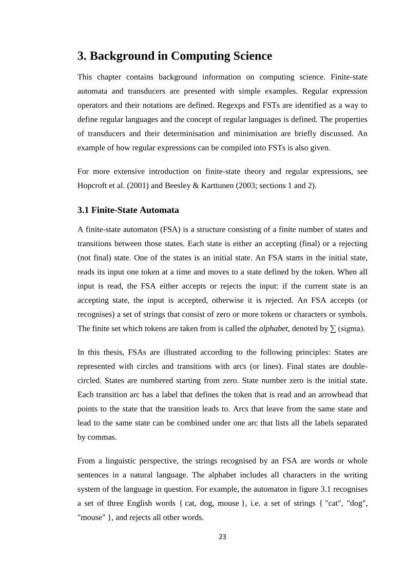
system of the language in question. For example, the automaton in figure 3.1 recognises
a set of three English words { cat, dog, mouse }, i.e. a set of strings { "cat", "dog",
"mouse" }, and rejects all other words.
24
Figure 3.1: An FSA that recognises a set of strings { "cat", "dog", "mouse" }.
As the FSA recognises only three words, the alphabet ∑ = { a, c, d, e, g, m, o, u, s, t } is
enough. In case we would like to add new words to the FSA, it is reasonable to expand
the alphabet so that it comprises all English letters: ∑ = { a, b, ... y, z }. Uppercase
letters are usually converted to lowercase in linguistic applications, if there is no
linguistic significance in the distinction.
3.2 Finite-State Transducers
Finite-State Transducers (FSTs) differ from finite-state automata in that they do not
only read their input but also produce output. For each read input token, a FST writes an
output token and moves to a state defined by the input and output tokens. An FST thus
accepts (or recognises) a set of string pairs. Actually, an FSA can be considered as an
FST if the input and output tokens are the same in each transition. Using this
interpretation, an FSA is an FST that reads its input and produces the same output.
FSTs are illustrated similarily as FSAs with the following added notations: Transition
arcs have a label that defines the token that is read and the token that is written. The
input and output tokens are separated by a colon, e.g. a:b defines a transition where an
input token a is read and an output token b is written. If the input and output tokens are
equal, the colon and one of the tokens can be omitted: a:a is the same as a.
At this point it is useful to introduce the notion of the empty token, epsilon. Epsilon is
very useful in constructing FSAs and necessary in FSTs that relate strings of different
lengths to each other. Epsilon is denoted with 0 (zero) in this thesis. In FSAs, epsilon
represents a free transition, i.e. a transition that can take place without reading any
25
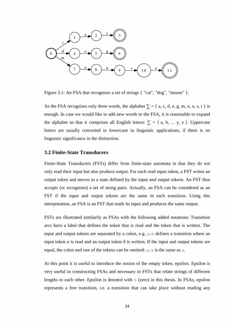
token. For example the automaton in figure 3.2 accepts both strings "color" and
"colour".
Figure 3.2: An FSA that recognises the strings "color" and "colour".
In FSTs, with epsilons it is possible to express a free transition either on the input,
output or both sides of a transition. In other words, it is possible to read a token without
writing any or vice versa. The next examples will illustrate how this feature can be used
in FSMs.
From a linguistic perspective, an FST is a relation between two sets of strings that
represent two levels of language. As said in section 2.2, it is common to view words as
having a surface and a deep level in linguistics. FSTs are a suitable way to encode this
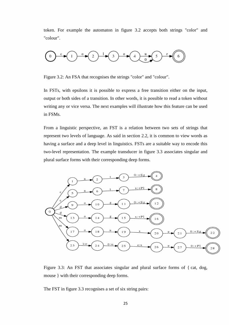
two-level representation. The example transducer in figure 3.3 associates singular and
plural surface forms with their corresponding deep forms.
Figure 3.3: An FST that associates singular and plural surface forms of { cat, dog,
mouse } with their corresponding deep forms.
The FST in figure 3.3 recognises a set of six string pairs:
26
{ <"cat","cat+Sg">, <"dog","dog+Sg">, <"mouse","mouse+Sg">,
<"cats","cat+Pl">, <"dogs","dog+Pl">, <"mice","mouse+Pl"> }.
If the FST is applied from input to output, it analyses surface forms to their base forms
and indicates whether the surface form is in the singular or plural with a +Sg or +Pl tag.
It can also generate singular and plural surface forms from a base form and a
morphological tag (+Sg, +Pl) if it is applied inversely. This transducer is a very simple
morphological analyser/generator.
3.3 FSTs and regular expressions
3.3.1 What are regular expressions and where are they used?
Regular expressions (regexps) are a means to define formal languages. A formal
language is a set of strings that consist of zero or more tokens or characters or symbols.
The finite set which the tokens are taken from is called the alphabet. As we can see, the
definition of a formal language is very similar to the definition of the strings recognised
by an FSA. Actually, both FSAs and regular expressions describe formal languages. It
can be shown that an FSA and a regular expression are equivalent formalisms of
defining formal languages. The equivalence also holds true for a FST and a regular
expression, if we just extend the definition of formal languages so that they are a set of
string pairs. Instead of states and transitions in an FSA/FST, a regular expression uses
tokens and operators to define formal languages. The operator notation is explained in
section 3.3.2.
Regular expressions can be viewed as a useful way to define transducers. It is often
simpler to write a regular expression and convert (or compile) it into a transducer than
to construct a transducer from scratch (more on compiling regexps to FSTs in section
3.4.1). Transducers, on the other hand, can be viewed as a way to implement regular
expressions. With their states and transitions, they are closer to computer programs -
that are actually almost like large finite-state automata. Regular expressions are a more
compact way to describe formal languages than drawing a transducer. However, often a
figure of a transducer is more illustrative than a regular expression.
3.3.2 Regexp notation
27
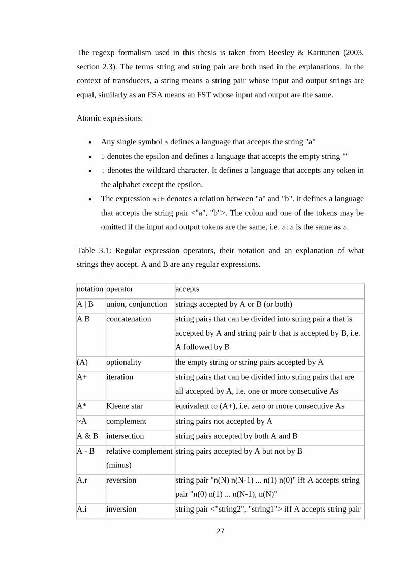
The regexp formalism used in this thesis is taken from Beesley & Karttunen (2003,
section 2.3). The terms string and string pair are both used in the explanations. In the
context of transducers, a string means a string pair whose input and output strings are
equal, similarly as an FSA means an FST whose input and output are the same.
Atomic expressions:
Any single symbol a defines a language that accepts the string "a"
0 denotes the epsilon and defines a language that accepts the empty string ""
? denotes the wildcard character. It defines a language that accepts any token in
the alphabet except the epsilon.
The expression a:b denotes a relation between "a" and "b". It defines a language
that accepts the string pair <"a", "b">. The colon and one of the tokens may be
omitted if the input and output tokens are the same, i.e. a:a is the same as a.
Table 3.1: Regular expression operators, their notation and an explanation of what
strings they accept. A and B are any regular expressions.
notation operator accepts
A | B union, conjunction strings accepted by A or B (or both)
A B concatenation string pairs that can be divided into string pair a that is
accepted by A and string pair b that is accepted by B, i.e.
A followed by B
(A) optionality the empty string or string pairs accepted by A
A+ iteration string pairs that can be divided into string pairs that are
all accepted by A, i.e. one or more consecutive As
A* Kleene star equivalent to (A+), i.e. zero or more consecutive As
~A complement string pairs not accepted by A
A & B intersection string pairs accepted by both A and B
A - B relative complement
(minus)
string pairs accepted by A but not by B
A.r reversion string pair "n(N) n(N-1) ... n(1) n(0)" iff A accepts string
pair "n(0) n(1) ... n(N-1), n(N)"
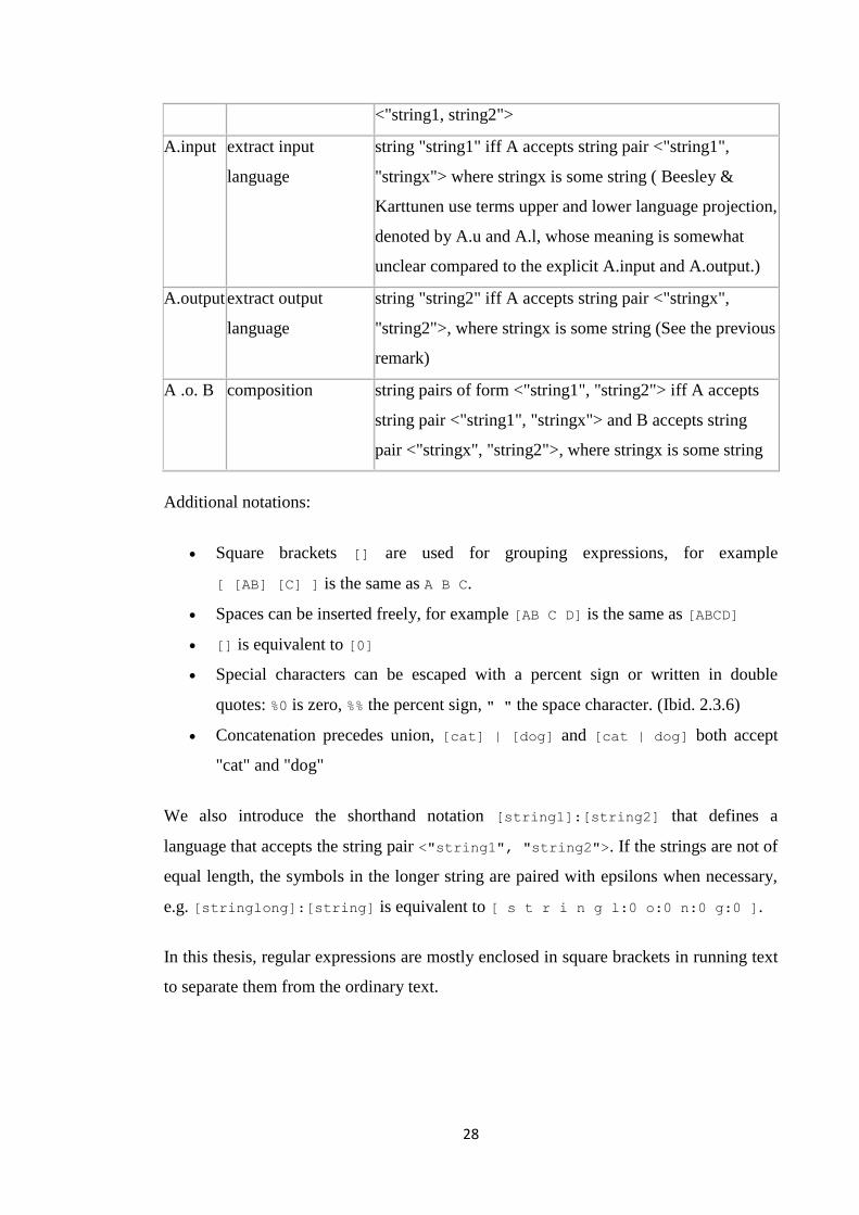
A.i inversion string pair <"string2", "string1"> iff A accepts string pair
28
<"string1, string2">
A.input extract input
language
string "string1" iff A accepts string pair <"string1",
"stringx"> where stringx is some string ( Beesley &
Karttunen use terms upper and lower language projection,
denoted by A.u and A.l, whose meaning is somewhat
unclear compared to the explicit A.input and A.output.)
A.output extract output
language
string "string2" iff A accepts string pair <"stringx",
"string2">, where stringx is some string (See the previous
remark)
A .o. B composition string pairs of form <"string1", "string2"> iff A accepts
string pair <"string1", "stringx"> and B accepts string
pair <"stringx", "string2">, where stringx is some string
Additional notations:
Square brackets [] are used for grouping expressions, for example
[ [AB] [C] ] is the same as A B C.
Spaces can be inserted freely, for example [AB C D] is the same as [ABCD]
[] is equivalent to [0]
Special characters can be escaped with a percent sign or written in double
quotes: %0 is zero, %% the percent sign, " " the space character. (Ibid. 2.3.6)
Concatenation precedes union, [cat] | [dog] and [cat | dog] both accept
"cat" and "dog"
We also introduce the shorthand notation [string1]:[string2] that defines a
language that accepts the string pair <"string1", "string2">. If the strings are not of
equal length, the symbols in the longer string are paired with epsilons when necessary,
e.g. [stringlong]:[string] is equivalent to [ s t r i n g l:0 o:0 n:0 g:0 ].
In this thesis, regular expressions are mostly enclosed in square brackets in running text
to separate them from the ordinary text.
29
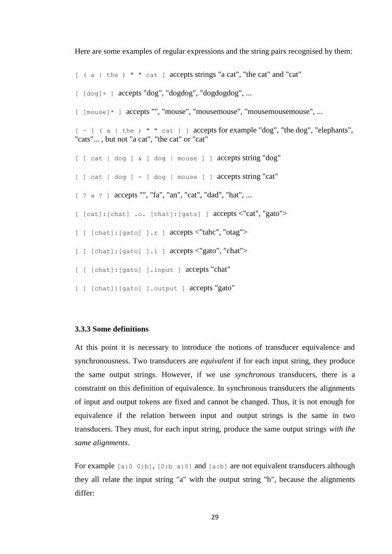
Here are some examples of regular expressions and the string pairs recognised by them:
[ ( a | the ) " " cat ] accepts strings "a cat", "the cat" and "cat"
[ [dog]+ ] accepts "dog", "dogdog", "dogdogdog", ...
[ [mouse]* ] accepts "", "mouse", "mousemouse", "mousemousemouse", ...
[ ~ [ ( a | the ) " " cat ] ] accepts for example "dog", "the dog", "elephants",
"cats"... , but not "a cat", "the cat" or "cat"
[ [ cat | dog ] & [ dog | mouse ] ] accepts string "dog"
[ [ cat | dog ] - [ dog | mouse ] ] accepts string "cat"
[ ? a ? ] accepts "", "fa", "an", "cat", "dad", "hat", ...
[ [cat]:[chat] .o. [chat]:[gato] ] accepts <"cat", "gato">
[ [ [chat]:[gato] ].r ] accepts <"tahc", "otag">
[ [ [chat]:[gato] ].i ] accepts <"gato", "chat">
[ [ [chat]:[gato] ].input ] accepts "chat"
[ [ [chat]:[gato] ].output ] accepts "gato"
3.3.3 Some definitions
At this point it is necessary to introduce the notions of transducer equivalence and
synchronousness. Two transducers are equivalent if for each input string, they produce
the same output strings. However, if we use synchronous transducers, there is a
constraint on this definition of equivalence. In synchronous transducers the alignments
of input and output tokens are fixed and cannot be changed. Thus, it is not enough for
equivalence if the relation between input and output strings is the same in two
transducers. They must, for each input string, produce the same output strings with the
same alignments.
For example [a:0 0:b], [0:b a:0] and [a:b] are not equivalent transducers although
they all relate the input string "a" with the output string "b", because the alignments
differ:
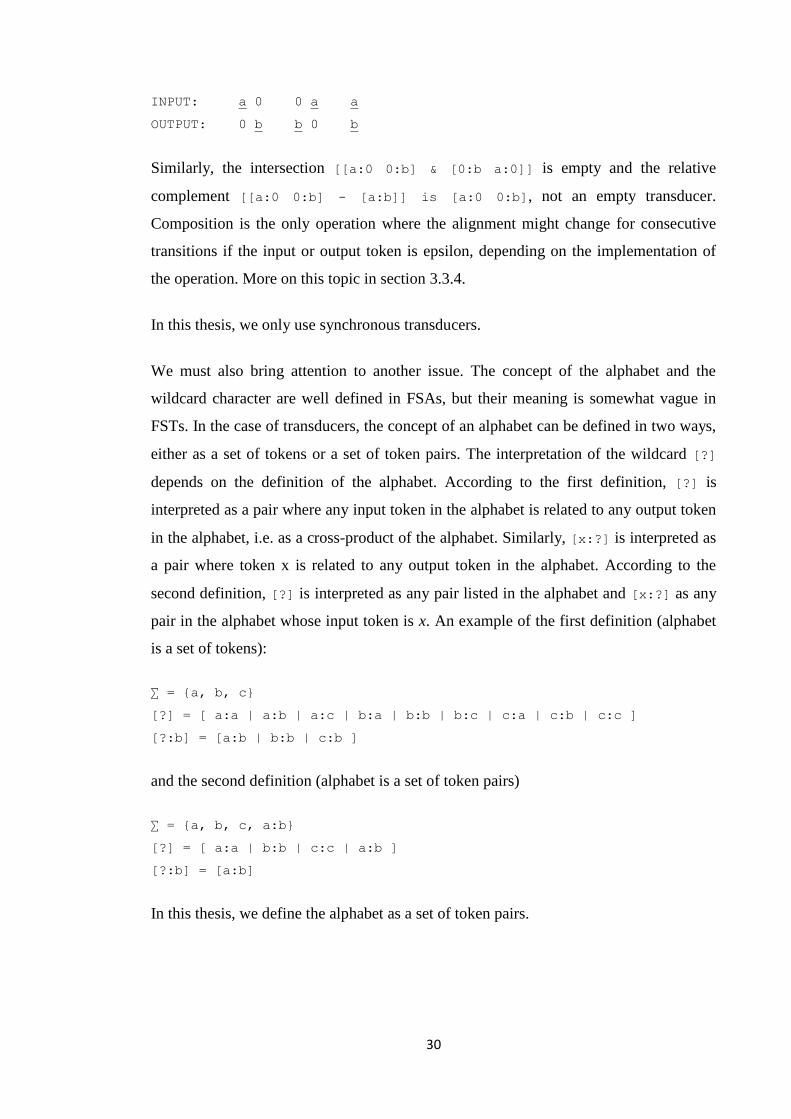
30
INPUT: a 0 0 a a
OUTPUT: 0 b b 0 b
Similarly, the intersection [[a:0 0:b] & [0:b a:0]] is empty and the relative
complement [[a:0 0:b] - [a:b]] is [a:0 0:b], not an empty transducer.
Composition is the only operation where the alignment might change for consecutive
transitions if the input or output token is epsilon, depending on the implementation of
the operation. More on this topic in section 3.3.4.
In this thesis, we only use synchronous transducers.
We must also bring attention to another issue. The concept of the alphabet and the
wildcard character are well defined in FSAs, but their meaning is somewhat vague in
FSTs. In the case of transducers, the concept of an alphabet can be defined in two ways,
either as a set of tokens or a set of token pairs. The interpretation of the wildcard [?]
depends on the definition of the alphabet. According to the first definition, [?] is
interpreted as a pair where any input token in the alphabet is related to any output token
in the alphabet, i.e. as a cross-product of the alphabet. Similarly, [x:?] is interpreted as
a pair where token x is related to any output token in the alphabet. According to the
second definition, [?] is interpreted as any pair listed in the alphabet and [x:?] as any
pair in the alphabet whose input token is x. An example of the first definition (alphabet
is a set of tokens):
∑ = {a, b, c}
[?] = [ a:a | a:b | a:c | b:a | b:b | b:c | c:a | c:b | c:c ]
[?:b] = [a:b | b:b | c:b ]
and the second definition (alphabet is a set of token pairs)
∑ = {a, b, c, a:b}
[?] = [ a:a | b:b | c:c | a:b ]
[?:b] = [a:b]
In this thesis, we define the alphabet as a set of token pairs.
31
3.3.4 Epsilon filtering
In composition, there are situations when two paths to be composed may yield several
alternative results. For instance the composition of transducers [ a:a b:0 c:0 d:d ]
and [ a:d 0:e d:a ] can be done in three ways:
[ a:d b:0 c:0 0:e d:a ]
[ a:d b:0 0:e c:0 d:a ]
[ a:d 0:e b:0 c:0 d:a ]
The reason for this ambiguity is that we are matching epsilons on the output side of the
first transducer and epsilons on the input side of the second transducer at the same time.
In the case of unweighted transducers multiple paths are not a problem, but in the case
of weighted transducers they can produce undesired results. A solution for this problem
is to insert an epsilon filter between the transducers that allows only one path, e.g. the
path where epsilons on the input side of the second transducer are traversed before
epsilons on the output side of the first transducer.
3.3.5 The limitations of regular expressions and FSTs
The ability of regular expressions and FSAs to express formal languages is extensive,
but not inclusive. For instance, it is not possible to define a formal language including
all palindromes with regular expressions or FSAs. Palindromes are strings of form " s(0)
s(1) ... s(N-1) s(N) ", where for each token s(n), s(n) is the same token as s(N-n). Strings
accepted by this formal language include for example "deleveled", "racecar" and
Finnish "saippuakauppias" ('soap vendor').
This language can be defined unambiguously, so it clearly exists. However, recognising
every possible palindrome requires an infinite amount of memory. A regular expression
cannot be infinitely long, as there cannot be infinite states in a finite-state automaton.
The subset of formal languages definable by FSAs and regular expressions is called
regular languages. Regular languages are enough for most practical applications
involving only the morphology of natural languages, i.e. languages spoken and written
by people.
32
3.4 Transducer operations and properties
Transducers do not have to be constructed from states and transitions. As we saw
earlier, FSTs can be compiled from regular expressions. It is also possible to construct
transducers from other transducers with operations. Because FSTs and regular
expressions are equivalent formalisms, the operators for regular expressions can also be
implemented for FSTs. The regexp operators introduced in the previous section also
exist for FSTs: union (conjunction), concatenation, optionality, iteration, Kleene star,
complement, intersection, relative complement (minus), reversion, inversion, extracting
input and output languages, composition. What has been said of these operators in table
3.1 also applies to transducers if we just interpret A and B as transducers instead of
regexps.
There exists optimising and testing operations that do not have a specific notation. The
most important of these are epsilon removal, determinisation, minimisation and
equivalence testing.
Removing epsilons from a transducer means creating an equivalent transducer that has
no transitions with [0:0] (epsilon) token pair. (Hopcroft et al., 2001 : 2.5.5)
Determinising a transducer means creating an equivalent epsilon-free transducer that
has no state that has two or more transitions with the same token pair. (Ibid: 2.3.5)
Minimising a transducer means creating an equivalent deterministic transducer with a
minimal number of states. It can be proven that for each transducer, there exists a
unique minimal transducer. (Ibid: 4.4.3) Thus, one way to test the equialence of two
transducers is to minimise them and test if they are the same transducer.
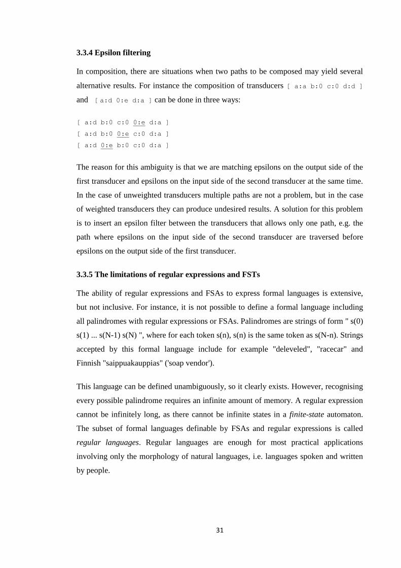
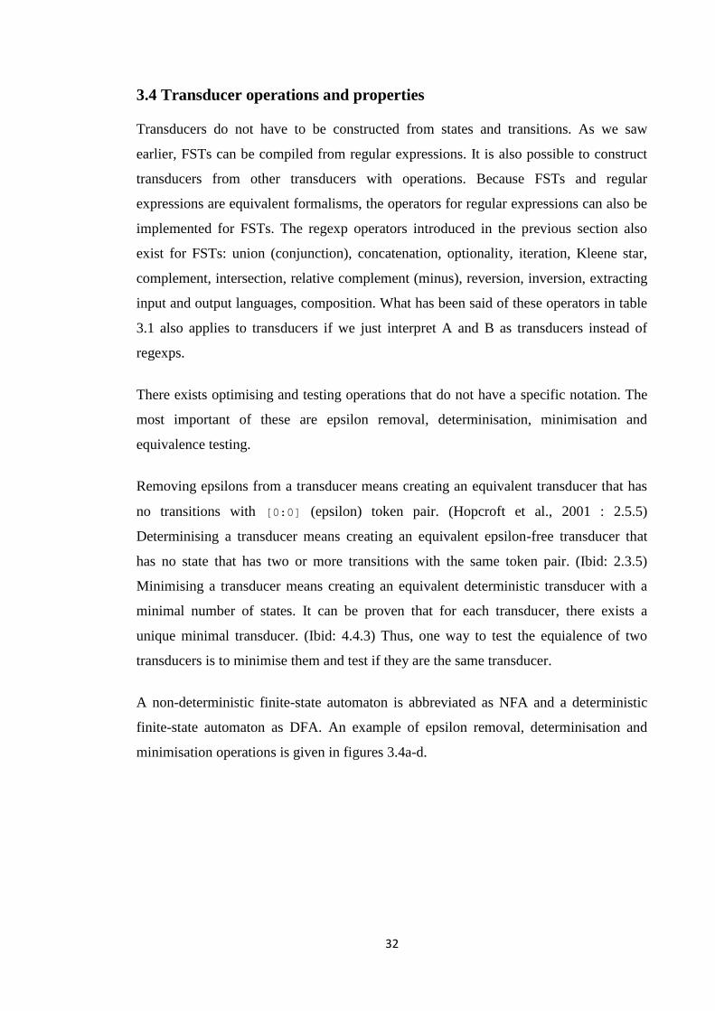
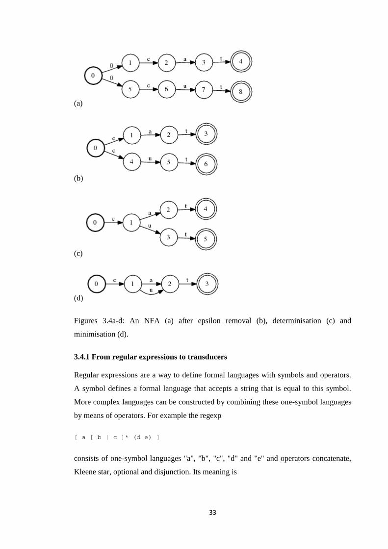
A non-deterministic finite-state automaton is abbreviated as NFA and a deterministic
finite-state automaton as DFA. An example of epsilon removal, determinisation and
minimisation operations is given in figures 3.4a-d.
33
(a)
(b)
(c)
(d)
Figures 3.4a-d: An NFA (a) after epsilon removal (b), determinisation (c) and
minimisation (d).
3.4.1 From regular expressions to transducers
Regular expressions are a way to define formal languages with symbols and operators.
A symbol defines a formal language that accepts a string that is equal to this symbol.
More complex languages can be constructed by combining these one-symbol languages
by means of operators. For example the regexp
[ a [ b | c ]* (d e) ]
consists of one-symbol languages "a", "b", "c", "d" and "e" and operators concatenate,
Kleene star, optional and disjunction. Its meaning is
34
"a" followed by any number of "b" or "c" followed by optional "d" or
"e"
or more precisely
"a" followed by ( (any number of ("b" or "c") ) followed by ( optional
("d" followed by "e") ) )
and more formally
"a" concatenated with ( (kleene star (disjunction of "b" and "c") )
concatenated with ( optional ("d" concatenated with "e") ) )
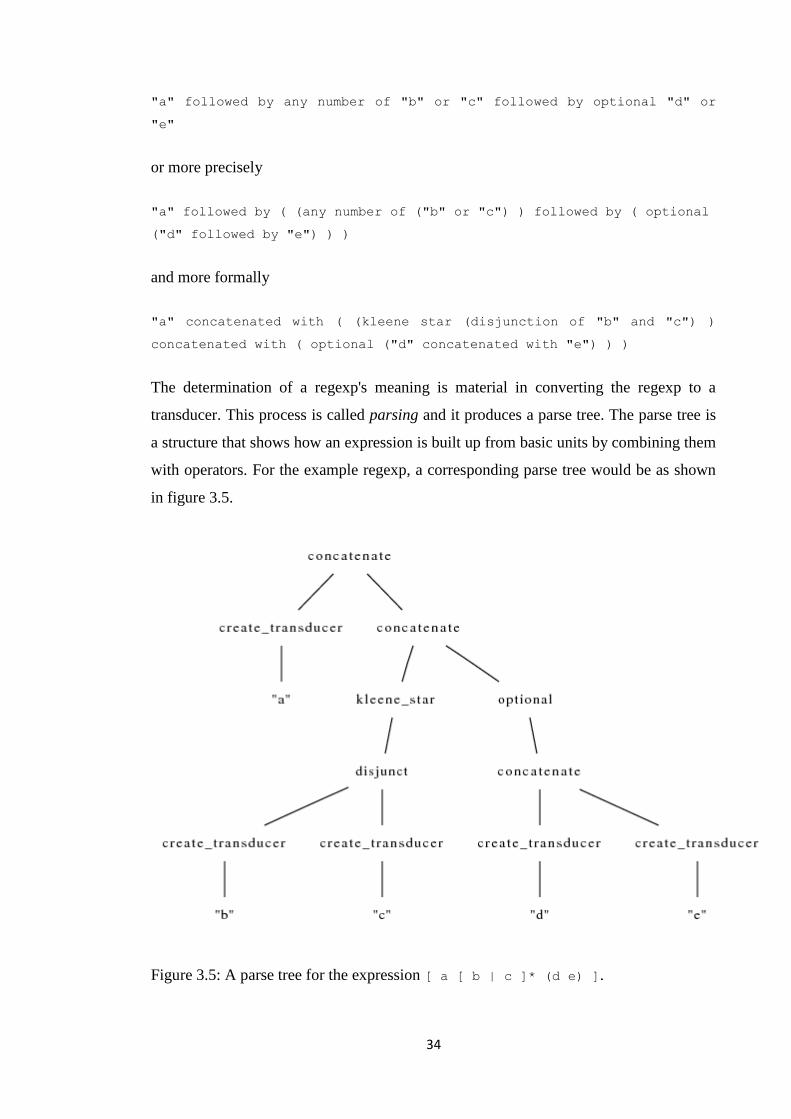
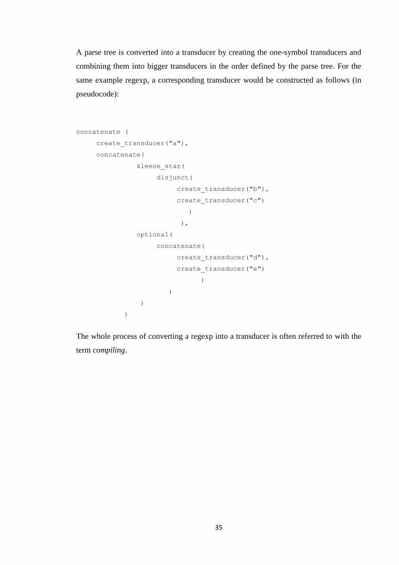
The determination of a regexp's meaning is material in converting the regexp to a
transducer. This process is called parsing and it produces a parse tree. The parse tree is
a structure that shows how an expression is built up from basic units by combining them
with operators. For the example regexp, a corresponding parse tree would be as shown
in figure 3.5.
Figure 3.5: A parse tree for the expression [ a [ b | c ]* (d e) ].
35
A parse tree is converted into a transducer by creating the one-symbol transducers and
combining them into bigger transducers in the order defined by the parse tree. For the
same example regexp, a corresponding transducer would be constructed as follows (in
pseudocode):
concatenate (
create_transducer("a"),
concatenate(
kleene_star(
disjunct(
create_transducer("b"),
create_transducer("c")
)
),
optional(
concatenate(
create_transducer("d"),
create_transducer("e")
)
)
)
)
The whole process of converting a regexp into a transducer is often referred to with the
term compiling.
36
4. Finite-State Morphologies (FSMs)
In the first two sections we describe what FSMs are and where they can be used. In the
third chapter we consider what a FSM should do if it encounters unknown words. In the
fourth section we explain how FSMs are created from lexicon and morphological rules.
We also motivate the use of rules with examples. In the fifth section we describe some
rule operators.
For a more extensive introduction to FSMs, see Beesley & Karttunen (2003) and
Koskenniemi (1996).
4.1 What are FSMs?
Finite-state morphologies are morphological dictionaries that are implemented with
finite-state transducers. A finite-state morphology usually implements a two-level
formalism, i.e. it can analyse surface forms to deep forms and generate surface forms
from deep forms. Surface forms are word forms as they appear in a text, e.g. He has
three mice. Deep forms present the same word forms as lexemes plus morphological
tags that can indicate the word class, inflection paradigm and inflection morphemes:
he+Pron have+Verb+Act+Ind+Pre+Sg+3 three+Num mouse+Noun+Pl.
In FSMs, the text is usually preprocessed so that punctuation marks are omitted and
upper case letters are converted to lower case. Extra line feeds are added so that there is
only one word per line. So, the previous example would actually be:
surface form deep form
he he+Pron
has have+Verb+Act+Ind+Pre+Sg+3
three three+Num
mice mouse+Noun+Pl
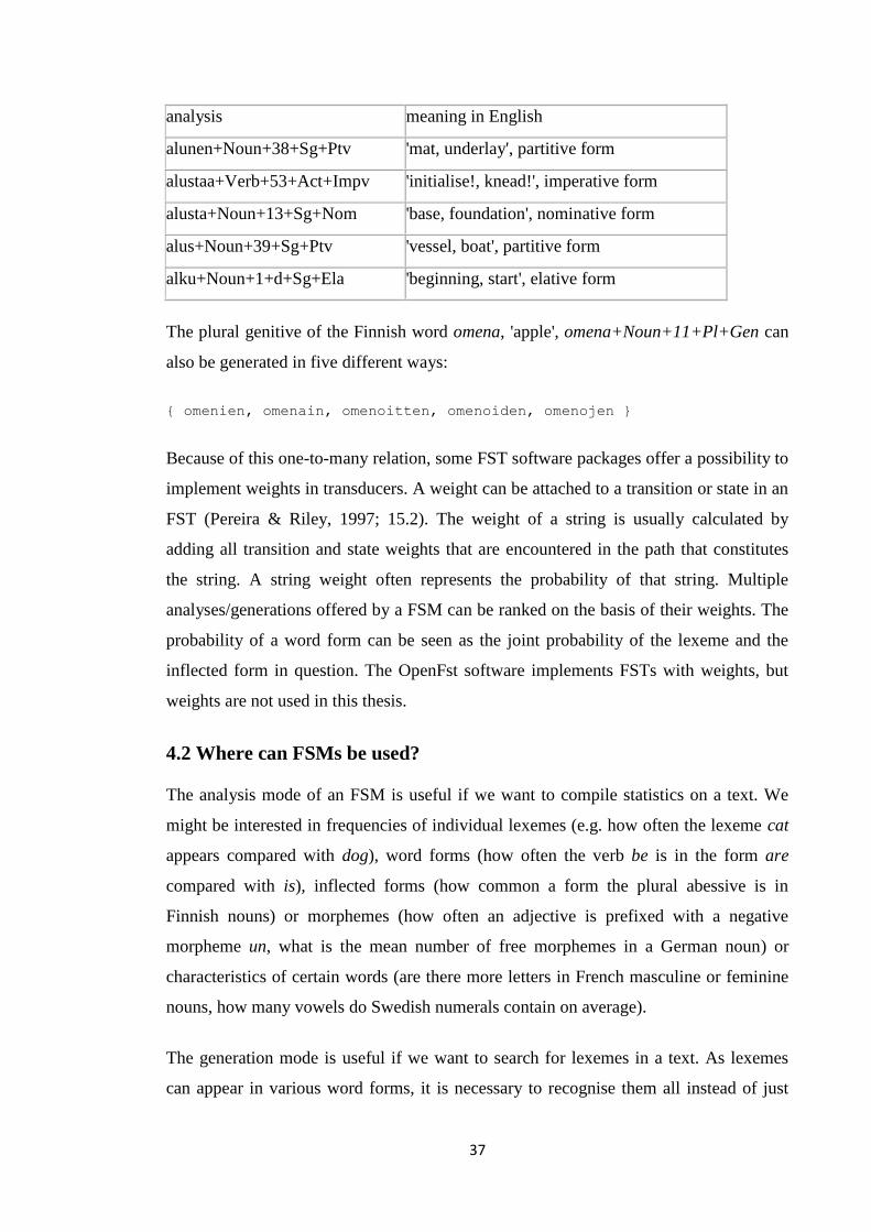
The relation between deep and surface forms is not always one-to-one. For example the
Finnish word form alusta can be analysed in five different ways:
37
analysis meaning in English
alunen+Noun+38+Sg+Ptv 'mat, underlay', partitive form
alustaa+Verb+53+Act+Impv 'initialise!, knead!', imperative form
alusta+Noun+13+Sg+Nom 'base, foundation', nominative form
alus+Noun+39+Sg+Ptv 'vessel, boat', partitive form
alku+Noun+1+d+Sg+Ela 'beginning, start', elative form
The plural genitive of the Finnish word omena, 'apple', omena+Noun+11+Pl+Gen can
also be generated in five different ways:
{ omenien, omenain, omenoitten, omenoiden, omenojen }
Because of this one-to-many relation, some FST software packages offer a possibility to
implement weights in transducers. A weight can be attached to a transition or state in an
FST (Pereira & Riley, 1997; 15.2). The weight of a string is usually calculated by
adding all transition and state weights that are encountered in the path that constitutes
the string. A string weight often represents the probability of that string. Multiple
analyses/generations offered by a FSM can be ranked on the basis of their weights. The
probability of a word form can be seen as the joint probability of the lexeme and the
inflected form in question. The OpenFst software implements FSTs with weights, but
weights are not used in this thesis.
4.2 Where can FSMs be used?
The analysis mode of an FSM is useful if we want to compile statistics on a text. We
might be interested in frequencies of individual lexemes (e.g. how often the lexeme cat
appears compared with dog), word forms (how often the verb be is in the form are
compared with is), inflected forms (how common a form the plural abessive is in
Finnish nouns) or morphemes (how often an adjective is prefixed with a negative
morpheme un, what is the mean number of free morphemes in a German noun) or
characteristics of certain words (are there more letters in French masculine or feminine
nouns, how many vowels do Swedish numerals contain on average).
The generation mode is useful if we want to search for lexemes in a text. As lexemes
can appear in various word forms, it is necessary to recognise them all instead of just
38
the base form. If a lexeme does not have many word forms, we can simply generate
them all. For instance, to identify all instances of the lexeme mouse in a text, we just
generate word forms mouse and mice and search the text for them. For Finnish that has
thousands of word forms for one lexeme, this approach would be too time-consuming.
A simple search method is to generate inflectional stems, i.e. stems where inflection
morphemes are added (Koskenniemi, 1996). For example, some of the word forms of
the lexeme hakea, 'to search' are haen, haet, hakee, haemme, haette, hakevat. We clearly
see that there are two stems hae- and hake-, so we can search the text for expressions
[hae?*] and [hake?*]. Of course this is a very vague search criterion and will produce
also false hits such as hakettaa, 'chip wood' (nothing to do with hakea) and hakemus,
'application' (actually etymologically related to hakea but it is a derived noun, not a verb
form). A more sophisticated search algorithm generates all word forms, but instead of
searching the text for each form individually, organises them in a search trie, a concise
structure where matching against words in the text can be done efficiently.
The search methods described above work in a situation where the amount of text is
large and will not be reused. If searchs are performed on the same text repeatedly, a
better approach is to analyse the entire text. As there might be several analyses for one
word form, they need to be either disambiguated manually or, if the analysing FSM
supports weights, listed in an order where the most probable analyses appear first. After
the text is analysed, each word form is represented as a deep form, i.e. by a lexeme plus
morphological tags. Then it is possible to search for lexemes directly with no need to
generate word forms.
4.3 Guessing unknown words
Ideally, a finite-state morphology should recognise and be able to generate all word
forms in a language. As real-life dictionaries cannot contain every word in a language,
the FSM will not always recognise a word. Therefore, it is important that the dictionary
application supports the feature of adding new words to the dictionary.
A morphological dictionary can also try to guess how a word form could be divided into
morphemes (Koskenniemi, 1996). It is possible that the dictionary finds some familiar
elements in the unknown word. The entire word is not necessarily unknown, but just
some of its morphemes. For example, the word ungwirphiest does not mean anything
39
but the dictionary could guess that the word contains a known prefix un denoting
negation, a known ending est denoting superlative plus an unknown root morpheme
gwirphy. The analysis offered would then be Neg+gwirphy+Adj+Sup meaning 'most
non-gwirphy'. The model followed here is clearly the inflectional paradigm of
adjectives ending in y, such as happy or easy. After making this educated guess, the
dictionary application should ask the user if he/she would like to add the newly found
word into the dictionary or reject it. So, if we pretend that the analysis is correct and
there exists an adjective gwirphy in English, we can add it to the dictionary. Next time
the dictionary encounters for example the word gwirphier, it analyses it directly as the
comparative of gwirphy, gwirphy+Adj+Comp, without using any guessing mechanism.
Guessing can also be applied to generation of word forms. If we pretend that quiwosh is
a verb and ask the dictionary to generate quiwosh+Verb+Act+Ind+Pre+Sg+3 it would
probably generate the word form quiwoshes, following the inflectional paradigm of
verbs as push - pushes. Although we have used nonsense words as examples, a guessing
mechanism is primarily intended for names, foreign loan words and newly coined words
that are not found in the dictionary. "Nonsense" words may of course occur in fictional
writing.
The morphological dictionaries used in this thesis do not implement a guessing
mechanism.
4.4 Compiling FSMs
4.4.1 The underlying software
The whole dictionary is basically a large regular expression that is compiled into a
transducer. There are many finite-state tools available, so usually a linguist who wants
to compile a dictionary will have to worry only about writing the regular expressions
correctly and let the finite-state tool perform the actual compilation. However, the
developers of the finite-state tool must take care of a number of things to build a
working compiler.
First of all, we need a regexp formalism that allows the user to define words and rules
and combine them with operators. This formalism can be considered a user interface to
the underlying software. The formalism must allow the user to construct transducers
40
from basic parts but also offer higher-level functions, e.g. creating rule transducers and
reading a list of words from a file. As the resulting transducer will be very big,
transducer (and possibly alphabet) variables are needed so that complex regular
expressions can be combined from smaller ones.
Secondly, the software needs a library that can handle transducers and perform
operations on them. The library must implement a data structure that represents a
transducer. It must also have a selection of functions that take one or more transducers
as their input, perform an operation on them (e.g. intersect, Kleene star, etc. ) and
produce a transducer as their output.
To unite the regexp formalism and the software itself into a compiler, we need a
program that can (1) parse the regexp and (2) construct the resulting transducer by
calling the functions in the library in the order defined by the parse tree. We also need a
program that can look up a word in the dictionary transducer, i.e. analyse a word form
or generate one. This is important both to the end-user using the dictionary and to the
linguist who wants to test that the dictionary works correctly.
4.4.2 The linguistic part
The way a morphological dictionary is compiled depends on the extent and complexity
of the morphology of the language in question. In case of English that has very few,
regular inflections, it is usually not too demanding just to list all word-forms in the
dictionary. In case of e.g. Finnish this approach is not possible. Finnish nouns have 15
cases in singular and plural constituting some thirty different word forms (some of
which are very rare). Finnish verbs have about fifty individual forms plus a number
forms consisting of an auxiliary verb and a participle such as olemme kuulleet, 'we have
heard' and olisi mennyt, '[he/she] would have gone'. Also many Romance languages
have a similar kind of verb inflection. It is evident that such extensive morphologies
cannot be compiled word form by word form.
The compounding mechanism can also be complex. In chapter 2.1.2 we mentioned that
Swedish three-part compounds need an additional infix between the second and third
morphemes. This is clearly a very regular and productive rule that can and must be
implemented in the dictionary in some other way than listing all possible three-part
compounds individually. However, the phonological variation in Swedish compounds
41
such as kyrko+gård, gatu+bild is not defineable by rules. Lexemes must have a tag that
indicates the phonological changes that happen when they are used in compounds.
German compounds do not always have clear rules of whether an infix is inserted
between morphemes as the example Arbeit+s+zimmer vs. Schlaf+zimmer showed. This
leaves no option but to list many compounds individually if this distinction is essential
for the application, e.g. for spell-checking. Alternatively, this may be left open if the
analysis of a possible misspelling is inconsequential, e.g. in information retrieval.
Some derivations are very productive but do not apply to every word or produce
meanings that are grammatical but strange. For instance, the Finnish suffix ja/jä that is
similar to English er in maker, writer, user etc. can be appended to almost all verbs, but
some combinations are still somewhat odd. voija 'that is able, canner' and sataja 'rainer'
are basically grammatical but it is not easy to find an example sentence where they
could be used. Some forms such as olija, 'who is, be+er' are not very sensible alone, but
appear frequently in compounds such as läsnä+olija, 'someone who is present'. It is
often difficult to manage these kinds of productive paradigms where the borderline
between the grammatical and ungrammatical is vague. Often we have to apply different
strategies for different applications.
Usually finite-state morphologies are not constructed word form by word form if the
language, or some parts of it, are more or less morphologically extensive or complex.
Instead, we have a lexicon and a set of morphological rules. The lexicon contains words
in their base form and possibly some tags that tell for example the word class and how
the word is inflected in various cases. In other words, the lexicon is a deep form
representation of lexemes. We also have a set of rules that tell how words in a certain
word class behave when inflected in a certain case. The rules are applied to the lexicon
resulting in a morphological dictionary. Usually the rules are not applied at run time but
the entire dictionary is compiled so that it contains all word forms and their
corresponding analyses. The resulting dictionary is large, but fast look-up is possible as
rules do not have to be applied individually for each dictionary search.
The compilation goes as follows (Beesley & Karttunen, 2003: 1.7): Each entry in the
lexicon is compiled into a transducer and all the transducers are disjuncted resulting in a
lexicon transducer. The morphological rules are compiled into transducers and the rule
transducers are combined through intersection or composition. The lexicon and the
42
resulting set of rule transducers are then composed resulting in a morphological
dictionary. It is also possible that only a part of the lexicon is extracted for applying a
certain rule set and the results are then disjuncted.
4.5 FSM rules
In chapter 2.2.3 we presented two-level rules. It is possible to express a similar kind of
rules with regular expressions and then convert the regular expressions into transducers.
The rules presented in 2.2.3 are obligatory and they must be applied in a certain order to
get the correct result as we saw in the examples presented. It is possible to construct a
more versatile rule formalism for regular expressions. We present two formalisms, the
Koskenniemi two-level rules and replace rules developed by Karttunen et al.
4.5.1 Two-level rules
Koskenniemi (1983) has implemented a two-level formalism where the validity and
scope of rules can be defined accurately.
The two-level rules are of the form
CP OP LC __ RC,
where CP is the mapping that occurs in the context between LC and RC. CP, LC and RC are
all regular expressions. LC and RC are automata expressing the left and the right context,
i.e. they map strings to themselves. CP is called the center of the rule. OP is an operator
that defines how the rule is applied. There exists three kind of rules: context restriction
rules, surface coercion rules and composite rules.
Context restriction rules are denoted as
CP => LC __ RC.
The meaning of the context restriction rule is that CP may occur only if it is enclosed in
the context LC __ RC. Other mappings than CP can also occur in the context LC __ RC,
but CP cannot occur outside the context LC __ RC.
Surface coercion rules are denoted as
43
CP <= LC __ RC.
The meaning of the surface coercion rule is that CP is the only mapping that can occur in
the context LC __ RC. Other mappings than CP cannot occur in the context LC __ RC,
but CP can occur also outside the context LC __ RC.
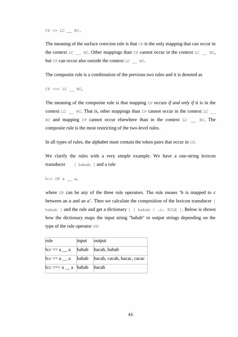
The composite rule is a combination of the previous two rules and it is denoted as
CP <=> LC __ RC,
The meaning of the composite rule is that mapping CP occurs if and only if it is in the
context LC __ RC. That is, other mappings than CP cannot occur in the context LC __
RC and mapping CP cannot occur elsewhere than in the context LC __ RC. The
composite rule is the most restricting of the two-level rules.
In all types of rules, the alphabet must contain the token pairs that occur in CP.
We clarify the rules with a very simple example. We have a one-string lexicon
transducer [ babab ] and a rule
b:c OP a __ a,
where OP can be any of the three rule operators. The rule means ‘b is mapped to c
between an a and an a’. Then we calculate the composition of the lexicon transducer [
babab ] and the rule and get a dictionary [ [ babab ] .o. RULE ]. Below is shown
how the dictionary maps the input string "babab" to output strings depending on the
type of the rule operator OP:
rule input output
b:c => a __ a babab bacab, babab
b:c <= a __ a babab bacab, cacab, bacac, cacac
b:c <=> a __ a babab bacab
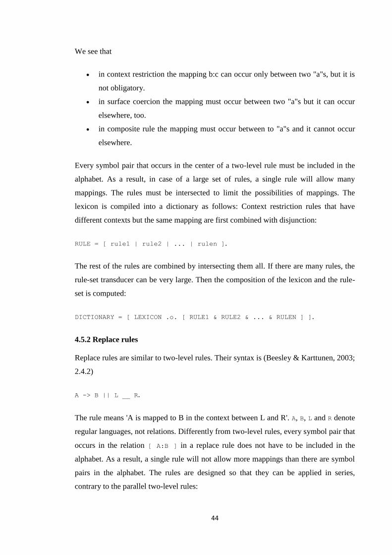
44
We see that
in context restriction the mapping b:c can occur only between two "a"s, but it is
not obligatory.
in surface coercion the mapping must occur between two "a"s but it can occur
elsewhere, too.
in composite rule the mapping must occur between to "a"s and it cannot occur
elsewhere.
Every symbol pair that occurs in the center of a two-level rule must be included in the
alphabet. As a result, in case of a large set of rules, a single rule will allow many
mappings. The rules must be intersected to limit the possibilities of mappings. The
lexicon is compiled into a dictionary as follows: Context restriction rules that have
different contexts but the same mapping are first combined with disjunction:
RULE = [ rule1 | rule2 | ... | rulen ].
The rest of the rules are combined by intersecting them all. If there are many rules, the
rule-set transducer can be very large. Then the composition of the lexicon and the rule-
set is computed:
DICTIONARY = [ LEXICON .o. [ RULE1 & RULE2 & ... & RULEN ] ].
4.5.2 Replace rules
Replace rules are similar to two-level rules. Their syntax is (Beesley & Karttunen, 2003;
2.4.2)
A -> B || L __ R.
The rule means 'A is mapped to B in the context between L and R'. A, B, L and R denote
regular languages, not relations. Differently from two-level rules, every symbol pair that
occurs in the relation [ A:B ] in a replace rule does not have to be included in the
alphabet. As a result, a single rule will not allow more mappings than there are symbol
pairs in the alphabet. The rules are designed so that they can be applied in series,
contrary to the parallel two-level rules:
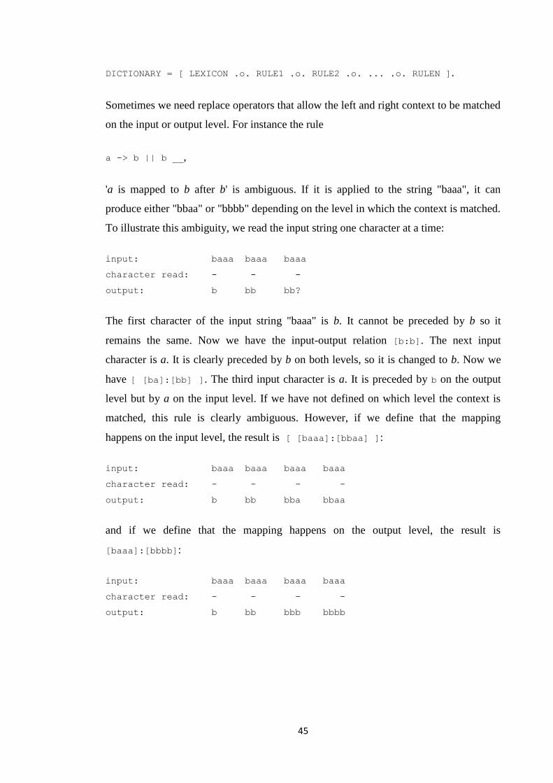
45
DICTIONARY = [ LEXICON .o. RULE1 .o. RULE2 .o. ... .o. RULEN ].
Sometimes we need replace operators that allow the left and right context to be matched
on the input or output level. For instance the rule
a -> b || b __,
'a is mapped to b after b' is ambiguous. If it is applied to the string "baaa", it can
produce either "bbaa" or "bbbb" depending on the level in which the context is matched.
To illustrate this ambiguity, we read the input string one character at a time:
input: baaa baaa baaa
character read: - - -
output: b bb bb?
The first character of the input string "baaa" is b. It cannot be preceded by b so it
remains the same. Now we have the input-output relation [b:b]. The next input
character is a. It is clearly preceded by b on both levels, so it is changed to b. Now we
have [ [ba]:[bb] ]. The third input character is a. It is preceded by b on the output
level but by a on the input level. If we have not defined on which level the context is
matched, this rule is clearly ambiguous. However, if we define that the mapping
happens on the input level, the result is [ [baaa]:[bbaa] ]:
input: baaa baaa baaa baaa
character read: - - - -
output: b bb bba bbaa
and if we define that the mapping happens on the output level, the result is
[baaa]:[bbbb]:
input: baaa baaa baaa baaa
character read: - - - -
output: b bb bbb bbbb
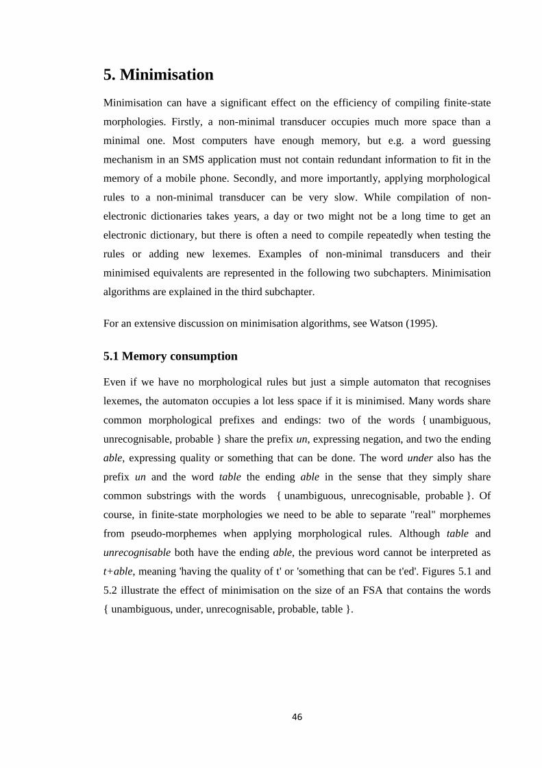
46
5. Minimisation
Minimisation can have a significant effect on the efficiency of compiling finite-state
morphologies. Firstly, a non-minimal transducer occupies much more space than a
minimal one. Most computers have enough memory, but e.g. a word guessing
mechanism in an SMS application must not contain redundant information to fit in the
memory of a mobile phone. Secondly, and more importantly, applying morphological
rules to a non-minimal transducer can be very slow. While compilation of non-
electronic dictionaries takes years, a day or two might not be a long time to get an
electronic dictionary, but there is often a need to compile repeatedly when testing the
rules or adding new lexemes. Examples of non-minimal transducers and their
minimised equivalents are represented in the following two subchapters. Minimisation
algorithms are explained in the third subchapter.
For an extensive discussion on minimisation algorithms, see Watson (1995).
5.1 Memory consumption
Even if we have no morphological rules but just a simple automaton that recognises
lexemes, the automaton occupies a lot less space if it is minimised. Many words share
common morphological prefixes and endings: two of the words { unambiguous,
unrecognisable, probable } share the prefix un, expressing negation, and two the ending
able, expressing quality or something that can be done. The word under also has the
prefix un and the word table the ending able in the sense that they simply share
common substrings with the words { unambiguous, unrecognisable, probable }. Of
course, in finite-state morphologies we need to be able to separate "real" morphemes
from pseudo-morphemes when applying morphological rules. Although table and
unrecognisable both have the ending able, the previous word cannot be interpreted as
t+able, meaning 'having the quality of t' or 'something that can be t'ed'. Figures 5.1 and
5.2 illustrate the effect of minimisation on the size of an FSA that contains the words
{ unambiguous, under, unrecognisable, probable, table }.
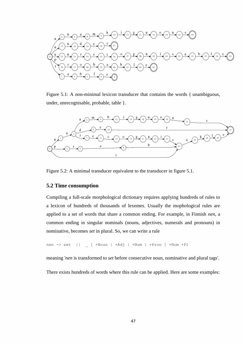
47
Figure 5.1: A non-minimal lexicon transducer that contains the words { unambiguous,
under, unrecognisable, probable, table }.
Figure 5.2: A minimal transducer equivalent to the transducer in figure 5.1.
5.2 Time consumption
Compiling a full-scale morphological dictionary requires applying hundreds of rules to
a lexicon of hundreds of thousands of lexemes. Usually the mophological rules are
applied to a set of words that share a common ending. For example, in Finnish nen, a
common ending in singular nominals (nouns, adjectives, numerals and pronouns) in
nominative, becomes set in plural. So, we can write a rule
nen -> set || _ [ +Noun | +Adj | +Num | +Pron ] +Nom +Pl
meaning 'nen is transformed to set before consecutive noun, nominative and plural tags'.
There exists hundreds of words where this rule can be applied. Here are some examples:
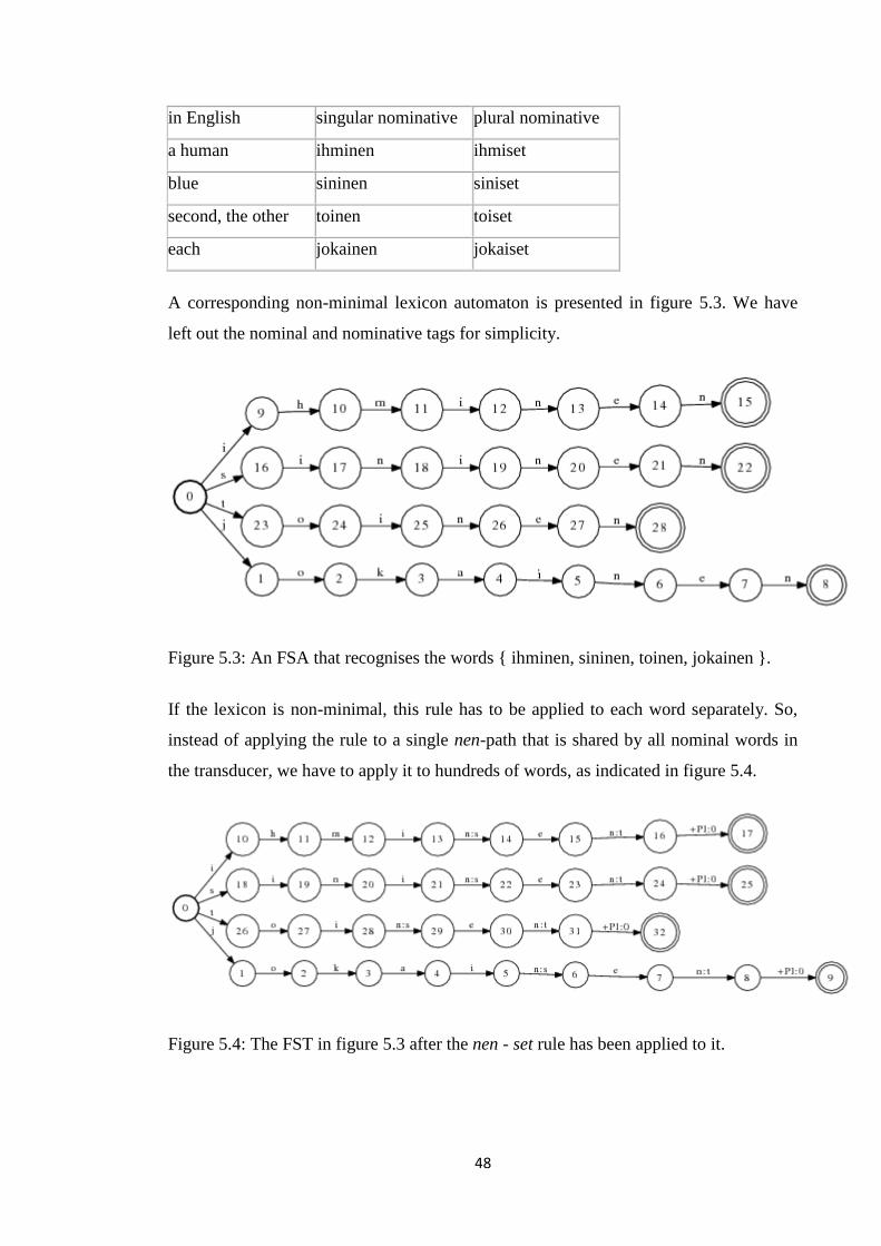
48
in English singular nominative plural nominative
a human ihminen ihmiset
blue sininen siniset
second, the other toinen toiset
each jokainen jokaiset
A corresponding non-minimal lexicon automaton is presented in figure 5.3. We have
left out the nominal and nominative tags for simplicity.
Figure 5.3: An FSA that recognises the words { ihminen, sininen, toinen, jokainen }.
If the lexicon is non-minimal, this rule has to be applied to each word separately. So,
instead of applying the rule to a single nen-path that is shared by all nominal words in
the transducer, we have to apply it to hundreds of words, as indicated in figure 5.4.
Figure 5.4: The FST in figure 5.3 after the nen - set rule has been applied to it.
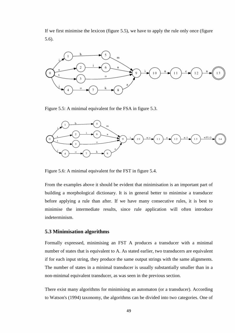
49
If we first minimise the lexicon (figure 5.5), we have to apply the rule only once (figure
5.6).
Figure 5.5: A minimal equivalent for the FSA in figure 5.3.
Figure 5.6: A minimal equivalent for the FST in figure 5.4.
From the examples above it should be evident that minimisation is an important part of
building a morphological dictionary. It is in general better to minimise a transducer
before applying a rule than after. If we have many consecutive rules, it is best to
minimise the intermediate results, since rule application will often introduce
indeterminism.
5.3 Minimisation algorithms
Formally expressed, minimising an FST A produces a transducer with a minimal
number of states that is equivalent to A. As stated earlier, two transducers are equivalent
if for each input string, they produce the same output strings with the same alignments.
The number of states in a minimal transducer is usually substantially smaller than in a
non-minimal equivalent transducer, as was seen in the previous section.
There exist many algorithms for minimising an automaton (or a transducer). According
to Watson's (1994) taxonomy, the algorithms can be divided into two categories. One of
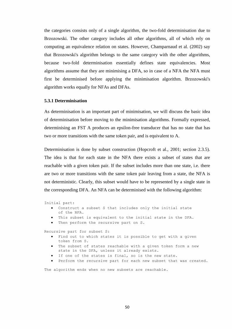
50
the categories consists only of a single algorithm, the two-fold determinisation due to
Brzozowski. The other category includes all other algorithms, all of which rely on
computing an equivalence relation on states. However, Champarnaud et al. (2002) say
that Brzozowski's algorithm belongs to the same category with the other algorithms,
because two-fold determinisation essentially defines state equivalencies. Most
algorithms assume that they are minimising a DFA, so in case of a NFA the NFA must
first be determinised before applying the minimisation algorithm. Brzozowski's
algorithm works equally for NFAs and DFAs.
5.3.1 Determinisation
As determinisation is an important part of minimisation, we will discuss the basic idea
of determinisation before moving to the minimisation algorithms. Formally expressed,
determinising an FST A produces an epsilon-free transducer that has no state that has
two or more transitions with the same token pair, and is equivalent to A.
Determinisation is done by subset construction (Hopcroft et al., 2001; section 2.3.5).
The idea is that for each state in the NFA there exists a subset of states that are
reachable with a given token pair. If the subset includes more than one state, i.e. there
are two or more transitions with the same token pair leaving from a state, the NFA is
not deterministic. Clearly, this subset would have to be represented by a single state in
the corresponding DFA. An NFA can be determinised with the following algorithm:
Initial part:
Construct a subset S that includes only the initial state
of the NFA.
This subset is equivalent to the initial state in the DFA.
Then perform the recursive part on S.
Recursive part for subset S:
Find out to which states it is possible to get with a given
token from S.
The subset of states reachable with a given token form a new
state in the DFA, unless it already exists.
If one of the states is final, so is the new state.
Perform the recursive part for each new subset that was created.
The algorithm ends when no new subsets are reachable.
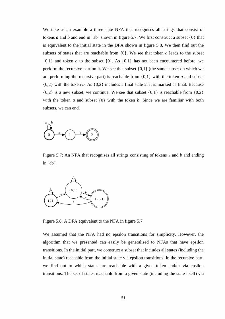
51
We take as an example a three-state NFA that recognises all strings that consist of
tokens a and b and end in "ab" shown in figure 5.7. We first construct a subset {0} that
is equivalent to the initial state in the DFA shown in figure 5.8. We then find out the
subsets of states that are reachable from {0}. We see that token a leads to the subset
{0,1} and token b to the subset {0}. As {0,1} has not been encountered before, we
perform the recursive part on it. We see that subset {0,1} (the same subset on which we
are performing the recursive part) is reachable from {0,1} with the token a and subset
{0,2} with the token b. As {0,2} includes a final state 2, it is marked as final. Because
{0,2} is a new subset, we continue. We see that subset {0,1} is reachable from {0,2}
with the token a and subset {0} with the token b. Since we are familiar with both
subsets, we can end.
Figure 5.7: An NFA that recognises all strings consisting of tokens a and b and ending
in "ab".
Figure 5.8: A DFA equivalent to the NFA in figure 5.7.
We assumed that the NFA had no epsilon transitions for simplicity. However, the
algorithm that we presented can easily be generalised to NFAs that have epsilon
transitions. In the initial part, we construct a subset that includes all states (including the
initial state) reachable from the initial state via epsilon transitions. In the recursive part,
we find out to which states are reachable with a given token and/or via epsilon
transitions. The set of states reachable from a given state (including the state itself) via
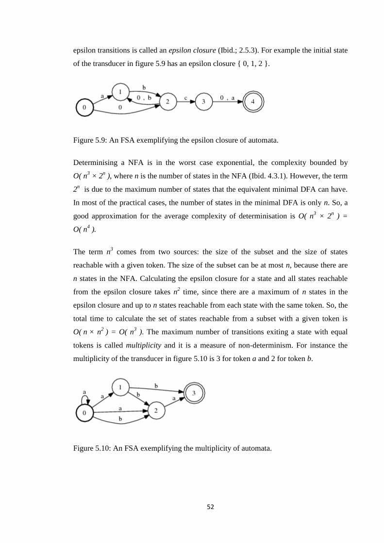
52
epsilon transitions is called an epsilon closure (Ibid.; 2.5.3). For example the initial state
of the transducer in figure 5.9 has an epsilon closure { 0, 1, 2 }.
Figure 5.9: An FSA exemplifying the epsilon closure of automata.
Determinising a NFA is in the worst case exponential, the complexity bounded by
O( n3 × 2
n ), where n is the number of states in the NFA (Ibid. 4.3.1). However, the term
2n is due to the maximum number of states that the equivalent minimal DFA can have.
In most of the practical cases, the number of states in the minimal DFA is only n. So, a
good approximation for the average complexity of determinisation is O( n3 × 2
n ) =
O( n4 ).
The term n3 comes from two sources: the size of the subset and the size of states
reachable with a given token. The size of the subset can be at most n, because there are
n states in the NFA. Calculating the epsilon closure for a state and all states reachable
from the epsilon closure takes n2 time, since there are a maximum of n states in the
epsilon closure and up to n states reachable from each state with the same token. So, the
total time to calculate the set of states reachable from a subset with a given token is
O( n × n2 ) = O( n
3 ). The maximum number of transitions exiting a state with equal
tokens is called multiplicity and it is a measure of non-determinism. For instance the
multiplicity of the transducer in figure 5.10 is 3 for token a and 2 for token b.
Figure 5.10: An FSA exemplifying the multiplicity of automata.
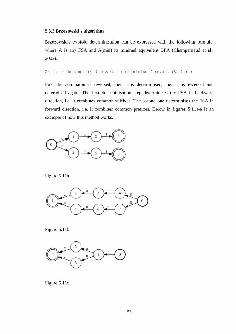
53
5.3.2 Brzozowski's algorithm
Brzozowski's twofold determinisation can be expressed with the following formula,
where A is any FSA and A(min) its minimal equivalent DFA (Champarnaud et al.,
2002):
A(min) = determinise ( revert ( determinise ( revert (A) ) ) )
First the automaton is reversed, then it is determinised, then it is reversed and
determised again. The first determinisation step determinises the FSA in backward
direction, i.e. it combines common suffixes. The second one determinises the FSA in
forward direction, i.e. it combines common prefixes. Below in figures 5.11a-e is an
example of how this method works.
Figure 5.11a
Figure 5.11b
Figure 5.11c
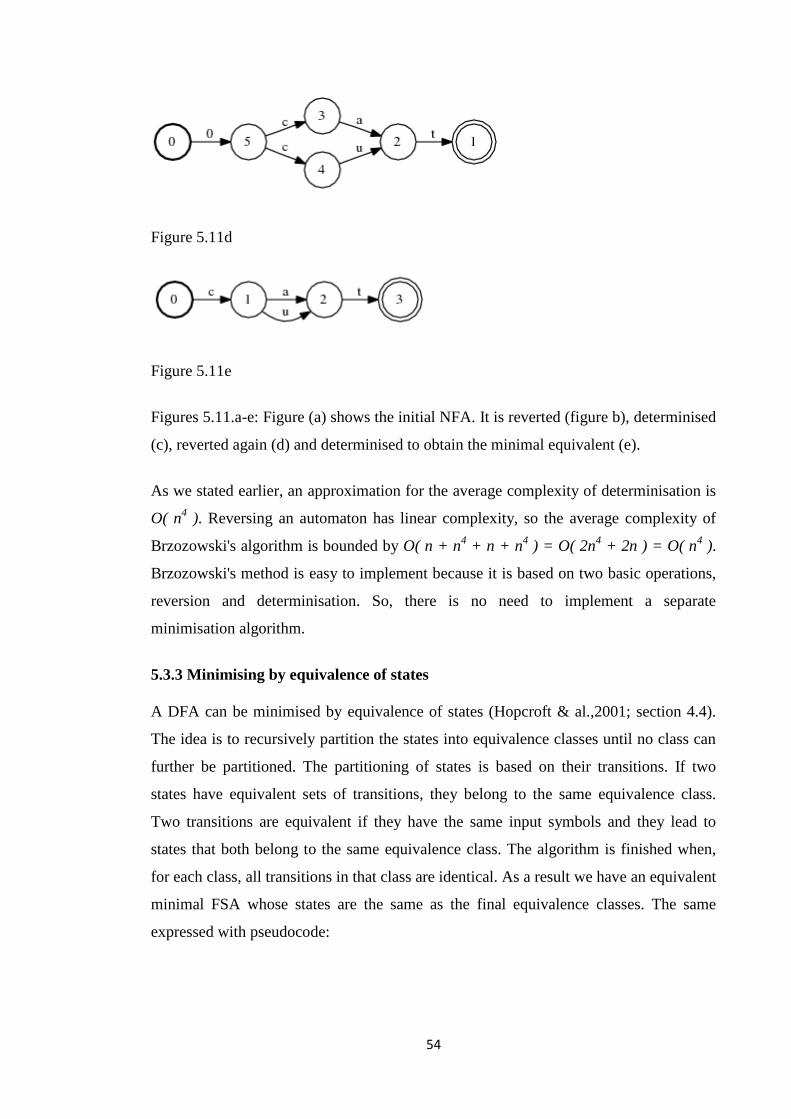
54
Figure 5.11d
Figure 5.11e
Figures 5.11.a-e: Figure (a) shows the initial NFA. It is reverted (figure b), determinised
(c), reverted again (d) and determinised to obtain the minimal equivalent (e).
As we stated earlier, an approximation for the average complexity of determinisation is
O( n4 ). Reversing an automaton has linear complexity, so the average complexity of
Brzozowski's algorithm is bounded by O( n + n4 + n + n
4 ) = O( 2n
4 + 2n ) = O( n
4 ).
Brzozowski's method is easy to implement because it is based on two basic operations,
reversion and determinisation. So, there is no need to implement a separate
minimisation algorithm.
5.3.3 Minimising by equivalence of states
A DFA can be minimised by equivalence of states (Hopcroft & al.,2001; section 4.4).
The idea is to recursively partition the states into equivalence classes until no class can
further be partitioned. The partitioning of states is based on their transitions. If two
states have equivalent sets of transitions, they belong to the same equivalence class.
Two transitions are equivalent if they have the same input symbols and they lead to
states that both belong to the same equivalence class. The algorithm is finished when,
for each class, all transitions in that class are identical. As a result we have an equivalent
minimal FSA whose states are the same as the final equivalence classes. The same
expressed with pseudocode:
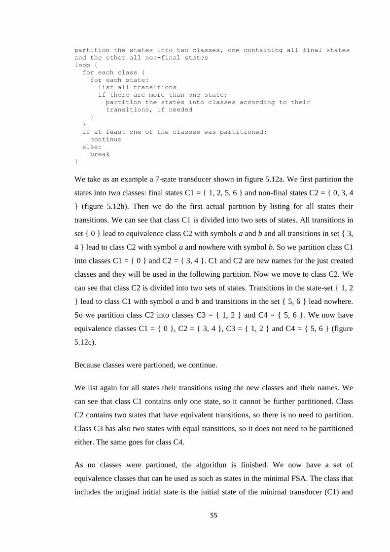
55
partition the states into two classes, one containing all final states
and the other all non-final states
loop {
for each class {
for each state:
list all transitions
if there are more than one state:
partition the states into classes according to their
transitions, if needed
}
}
if at least one of the classes was partitioned:
continue
else:
break
}
We take as an example a 7-state transducer shown in figure 5.12a. We first partition the
states into two classes: final states C1 = { 1, 2, 5, 6 } and non-final states C2 = { 0, 3, 4
} (figure 5.12b). Then we do the first actual partition by listing for all states their
transitions. We can see that class C1 is divided into two sets of states. All transitions in
set { 0 } lead to equivalence class C2 with symbols a and b and all transitions in set { 3,
4 } lead to class C2 with symbol a and nowhere with symbol b. So we partition class C1
into classes C1 = { 0 } and C2 = { 3, 4 }. C1 and C2 are new names for the just created
classes and they will be used in the following partition. Now we move to class C2. We
can see that class C2 is divided into two sets of states. Transitions in the state-set { 1, 2
} lead to class C1 with symbol a and b and transitions in the set { 5, 6 } lead nowhere.
So we partition class C2 into classes C3 = { 1, 2 } and C4 = { 5, 6 }. We now have
equivalence classes C1 = { 0 }, C2 = { 3, 4 }, C3 = { 1, 2 } and C4 = { 5, 6 } (figure
5.12c).
Because classes were partioned, we continue.
We list again for all states their transitions using the new classes and their names. We
can see that class C1 contains only one state, so it cannot be further partitioned. Class
C2 contains two states that have equivalent transitions, so there is no need to partition.
Class C3 has also two states with equal transitions, so it does not need to be partitioned
either. The same goes for class C4.
As no classes were partioned, the algorithm is finished. We now have a set of
equivalence classes that can be used as such as states in the minimal FSA. The class that
includes the original initial state is the initial state of the minimal transducer (C1) and
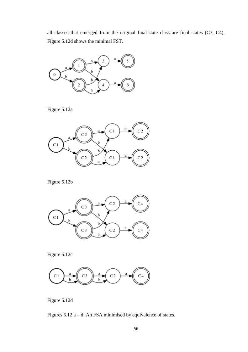
56
all classes that emerged from the original final-state class are final states (C3, C4).
Figure 5.12d shows the minimal FST.
Figure 5.12a
Figure 5.12b
Figure 5.12c
Figure 5.12d
Figures 5.12 a – d: An FSA minimised by equivalence of states.
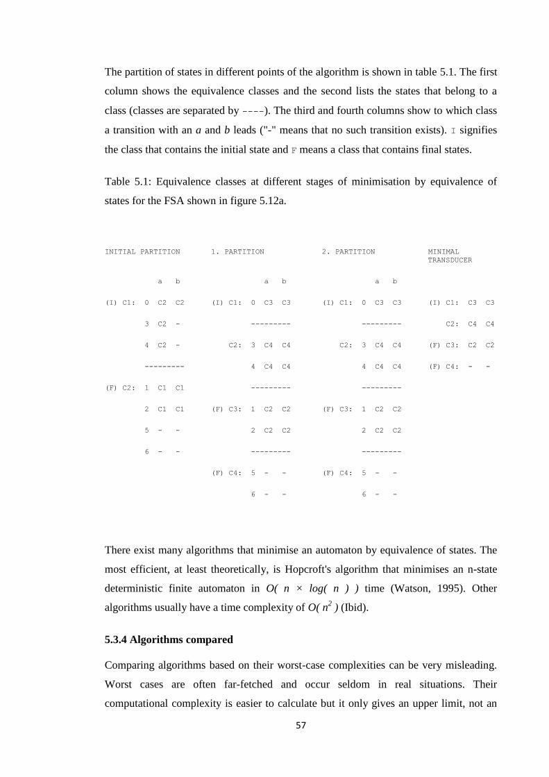
57
The partition of states in different points of the algorithm is shown in table 5.1. The first
column shows the equivalence classes and the second lists the states that belong to a
class (classes are separated by ----). The third and fourth columns show to which class
a transition with an a and b leads ("-" means that no such transition exists). I signifies
the class that contains the initial state and F means a class that contains final states.
Table 5.1: Equivalence classes at different stages of minimisation by equivalence of
states for the FSA shown in figure 5.12a.
INITIAL PARTITION 1. PARTITION 2. PARTITION MINIMAL
TRANSDUCER
a b a b a b
(I) C1: 0 C2 C2 (I) C1: 0 C3 C3 (I) C1: 0 C3 C3 (I) C1: C3 C3
3 C2 - --------- --------- C2: C4 C4
4 C2 - C2: 3 C4 C4 C2: 3 C4 C4 (F) C3: C2 C2
--------- 4 C4 C4 4 C4 C4 (F) C4: - -
(F) C2: 1 C1 C1 --------- ---------
2 C1 C1 (F) C3: 1 C2 C2 (F) C3: 1 C2 C2
5 - - 2 C2 C2 2 C2 C2
6 - - --------- ---------
(F) C4: 5 - - (F) C4: 5 - -
6 - - 6 - -
There exist many algorithms that minimise an automaton by equivalence of states. The
most efficient, at least theoretically, is Hopcroft's algorithm that minimises an n-state
deterministic finite automaton in O( n × log( n ) ) time (Watson, 1995). Other
algorithms usually have a time complexity of O( n2 ) (Ibid).
5.3.4 Algorithms compared
Comparing algorithms based on their worst-case complexities can be very misleading.
Worst cases are often far-fetched and occur seldom in real situations. Their
computational complexity is easier to calculate but it only gives an upper limit, not an
58
estimate for the average case. We need a large sample of real test instances to determine
whether one algorithm is more efficient than the other. Often it turns out that one
algorithm works better in certain circumstances and the other in other circumstances. In
the case of automaton algorithms, the size of the automaton, the amount of transitions
per state, the proportion of final states and the degree of non-determinism and cyclicity
are examples of properties that might affect the performance of a given algorithm. We
clearly cannot state that HOP is better than BRZ only on the basis of their theoretical
complexities O( n × log( n ) ) vs. O( n4 ).
We must also remember that BRZ works for NFAs while using HOP the NFA must first
be determinised. So, in the general case, we should write the complexity of HOP as the
sum of determinisation and the HOP itself: O( n × log( n ) + n4 ) = O( n
4 ). Then, for
any NFA, the complexities of BRZ and HOP are identical. Of course the
determinisation steps in BRZ and HOP do not necessarily take an equal amount of time.
Although HOP's only determinisation step and BRZ's second determinisation step both
determinise the NFA in forward direction, they are not comparable operations. In BRZ
the NFA has already been changed due to the backward determinisation and two
reversions. Neither is it likely that determinising the transducer in forward and
backward direction in BRZ are equally demanding tasks.
Despite its worst-case complexity O( n4 ) BRZ is often said to perform well in practice
(Castiglione et al., 2008), (Champarnaud et al., 2002), (Watson, 1995) and even
outperform HOP (Almeida et al., 2007). However, there are no studies where BRZ and
HOP would have been tested with linguistic data.
Tabakov & Vardi (2005) have compared the performance of Brzozowski's and
Hopcroft's algorithms based on their performance on randomly generated NFAs.
Performance was defined in terms of the time to calculate the minimised DFA. The
properties of the NFAs were varied by controlling their density and a graph showing the
time spent on minimisation as the function of density was plotted. The densities were
the density of the accepting states (i.e. ratio of accepting states to total states) and the
density of transitions. Transition density is a measure of indeterminism as it gives an
average for number of transitions with equal letters leaving from a state.
59
It was shown that Hopcroft's algorithm generally performs better than Brzozowski's, but
the latter performs better at high transition densities. The algorithms perform equally on
NFAs whose transition densities were below 1. On transition densities between 1 and
1.5 HOP was better than BRZ, which had a sharp and high peak at 1.25. If transition
density was above 1.5, BRZ was faster. HOP had its peak value at 1.5, BRZ at 1.25.
The test NFAs had 30 or 40 states and a binary alphabet ∑ = { 0, 1 }.
Watson (1995) has compared the performance of five minimisation algorithms in his
thesis. The test NFAs were constructed from regular expressions. They had at most 25
states, were rather sparse and their alphabet consisted of the entire ASCII set. The
algorithms performed equally on NFAs having at most 10 states. On larger NFAs BRZ
was more efficient than HOP. However, Watson says that with its excellent theoretical
running time, HOP will outperform the BRZ on very large DFAs.
With both Tabakov & Vardi (2005) and Watson (1995) the problem is that their test
transducers are very small, having a maximum of 40 states. The results can be useful in
other areas, e.g. in electronics when minimising circuit boards. However, they cannot
necessarily be generalised to the field of computational linguistics where automata can
have millions of states. There is clearly a need for benchmarking both BRZ and HOP on
real linguistic data.
60
6. Data
We have as our testing data two finite-state morphologies, OMorFi and Morphisto.
They are both written with the SFST programming language which is part of the SFST
tools. The SFST programming language is presented in the first section. OMorFi and
Morphisto are presented in the second and third sections.
6.1 SFST programming language (SFST-PL)
An SFST program is essentially a regular expression that is compiled into an SFST
transducer. The SFST-PL regular expression formalism is slightly different from the
one presented in chapter 2 but implements the same features. Basic operators, including
union, concatenation, optionality, iteration, Kleene star, complement, intersection,
relative complement, composition, reversion, inversion, extraction of input or output
language and some extra operators plus the wildcard character are all part of the SFST-
PL. SFST-PL also provides two-level and replace rule operators and an operator to read
lexicon entries from a lexicon.
The SFST alphabet contains a set of symbol pairs which is required for the
interpretation of the wildcard symbol. The definition of an alphabet is also required by
the negation operator and the two-level rules. The alphabet can be redefined at any point
in the program. Multicharacter symbols and grammatical tags are enclosed in brackets,
e.g. the string "mew+Pres+Sg+3" would be "mew<Pres><Sg><3>" in SFST syntax.
The epsilon is denoted by "<>". Comments start with a per cent sign.
The following very simple example is taken from the SFST manual. It shows the
implementation of an infectional component for English adjectives such as easy, late, or
dark. It will correctly analyse forms such as easier, latest, or darkest and produce the
analyses easy<ADJ><comp>, late<ADJ><sup> and dark<ADJ><sup>.
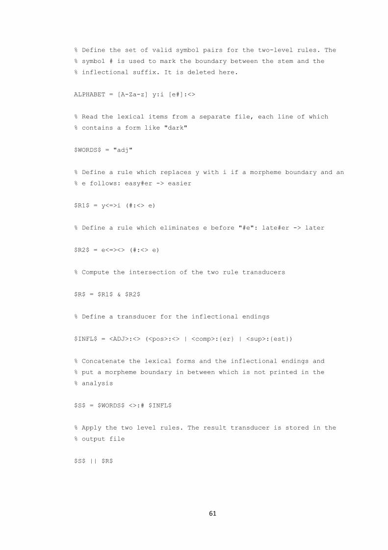
61
% Define the set of valid symbol pairs for the two-level rules. The
% symbol # is used to mark the boundary between the stem and the
% inflectional suffix. It is deleted here.
ALPHABET = [A-Za-z] y:i [e#]:<>
% Read the lexical items from a separate file, each line of which
% contains a form like "dark"
$WORDS$ = "adj"
% Define a rule which replaces y with i if a morpheme boundary and an
% e follows: easy#er -> easier
$R1$ = y<=>i (#:<> e)
% Define a rule which eliminates e before "#e": late#er -> later
$R2$ = e<=><> (#:<> e)
% Compute the intersection of the two rule transducers
$R$ = $R1$ & $R2$
% Define a transducer for the inflectional endings
$INFL$ = <ADJ>:<> (<pos>:<> | <comp>:{er} | <sup>:{est})
% Concatenate the lexical forms and the inflectional endings and
% put a morpheme boundary in between which is not printed in the
% analysis
$S$ = $WORDS$ <>:# $INFL$
% Apply the two level rules. The result transducer is stored in the
% output file
$S$ || $R$
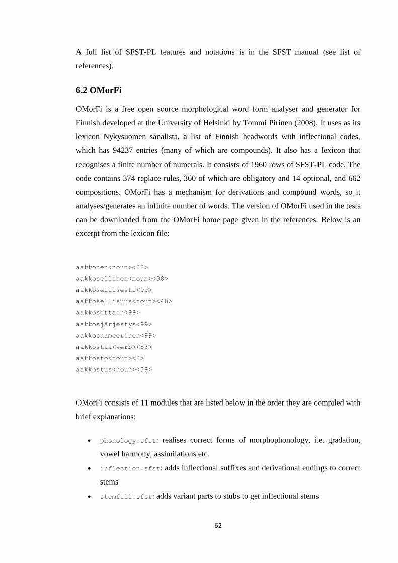
62
A full list of SFST-PL features and notations is in the SFST manual (see list of
references).
6.2 OMorFi
OMorFi is a free open source morphological word form analyser and generator for
Finnish developed at the University of Helsinki by Tommi Pirinen (2008). It uses as its
lexicon Nykysuomen sanalista, a list of Finnish headwords with inflectional codes,
which has 94237 entries (many of which are compounds). It also has a lexicon that
recognises a finite number of numerals. It consists of 1960 rows of SFST-PL code. The
code contains 374 replace rules, 360 of which are obligatory and 14 optional, and 662
compositions. OMorFi has a mechanism for derivations and compound words, so it
analyses/generates an infinite number of words. The version of OMorFi used in the tests
can be downloaded from the OMorFi home page given in the references. Below is an
excerpt from the lexicon file:
aakkonen<noun><38>
aakkosellinen<noun><38>
aakkosellisesti<99>
aakkosellisuus<noun><40>
aakkosittain<99>
aakkosjärjestys<99>
aakkosnumeerinen<99>
aakkostaa<verb><53>
aakkosto<noun><2>
aakkostus<noun><39>
OMorFi consists of 11 modules that are listed below in the order they are compiled with
brief explanations:
phonology.sfst: realises correct forms of morphophonology, i.e. gradation,
vowel harmony, assimilations etc.
inflection.sfst: adds inflectional suffixes and derivational endings to correct
stems
stemfill.sfst: adds variant parts to stubs to get inflectional stems
63
stubify.sfst: replaces variant parts of dictionary forms with zeros to get
invariant stub forms
find-gradation.sfst: finds and marks gradation on dictionary word.
plurale-tantum.sfst: finds plurale tantum words from root lexicon and
recreates singular forms
The lexicon building uses these six modules to get from lexicon forms to full
morphological analyser.
omorfi_1.sfst: reads lexica from sfstlex type files, applies the above
mentioned six modules in order and produces first pass inflectional forms.
omorfi_2.sfst: reads participles, comparatives, superlatives and derivations
from the first pass inflectional forms and produces second pass inflectional
forms
exceptions.sfst: reads exceptional word forms from the exception lexicon
and processes them through partial inflection.
compounds.sfst: reads word forms from previous modules and combines them
using compounding rules.
omorfi.sfst: collects inflectional forms from modules omorfi_1, omorfi_2,
exceptions and compounds.
6.3 Morphisto
Morphisto is a morphological analyser for German. It is based on the open-source
SMOR morphology for the German language developed by the University of Stuttgart.
Morphisto can be downloaded from Morphisto home page given in the list of
references. The lexicon has 19618 entries (some of which are compounds) plus an
infinite number of numerals. Morphisto also has a mechanism for derivations and
compound words, so it analyses/generates an infinite number of words. It has 4673 rows
of SFST-PL code. It has 120 two-level rules, 76 of which are contexts restrictions and
44 composite rules, and 119 compositions. The two-level rules are applied as if they
were replace rules, however. Morphisto is not divided into modules as clearly as
OMorFi. Below is an excerpt from the lexicon file:
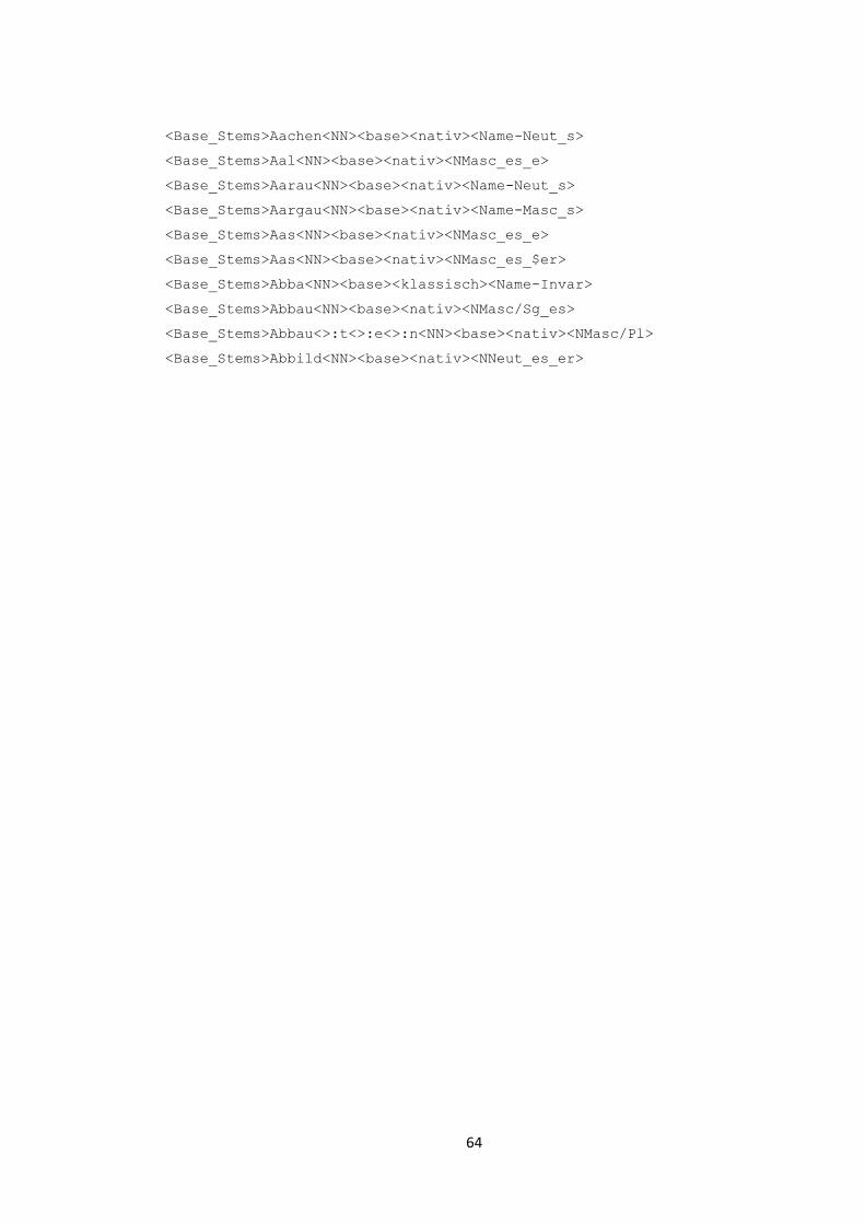
64
<Base_Stems>Aachen<NN><base><nativ><Name-Neut_s>
<Base_Stems>Aal<NN><base><nativ><NMasc_es_e>
<Base_Stems>Aarau<NN><base><nativ><Name-Neut_s>
<Base_Stems>Aargau<NN><base><nativ><Name-Masc_s>
<Base_Stems>Aas<NN><base><nativ><NMasc_es_e>
<Base_Stems>Aas<NN><base><nativ><NMasc_es_$er>
<Base_Stems>Abba<NN><base><klassisch><Name-Invar>
<Base_Stems>Abbau<NN><base><nativ><NMasc/Sg_es>
<Base_Stems>Abbau<>:t<>:e<>:n<NN><base><nativ><NMasc/Pl>
<Base_Stems>Abbild<NN><base><nativ><NNeut_es_er>
65
7. Tests
In the preface section, we describe the software and tools that are used in the tests and
outline a testing strategy. In the first section, we compile OMorFi and Morphisto with
SFST, unweighted HFST and weighted HFST to see if their compilation times differ. In
the second section, we profile unweighted and weighted HFST in more detail to see
where these differences occur. It turns out that the minimisation algorithms, BRZ in
unweighted HFST and HOP in weighted HFST, are responsible for most of the
differences in performance. In the third section, we compile OMorFi and Morphisto
again and change only the minimisation algorithm. We see that the differences still
exist.
In the fourth section, we find out what kinds of transducers are slow to minimise with
BRZ and what kind of transducers with HOP. The results lead us to our hypothesis
about cyclicity. In the fifth section, we examine how the properties of transducers
change in the determinisations that are part of BRZ and HOP. In the sixth section, we
test the cyclicity hypothesis with simple data. The hypothesis seems to be correct.
7.1 The tools and strategy
7.1.1 The software and tools
The Helsinki Finite-State Transducer (HFST) software is intended for the
implementation of morphological analysers and other tools which are based on
weighted and unweighted finite-state transducer technology. The work is licensed under
a GNU Lesser General Public License v3.0. The HFST software can be used through an
API or command line tools.
The HFST transducer library offers two modes of operation, an unweighted and a
weighted one. The unweighted part of the library is based on SFST and the weighted
one on OpenFst. SFST and OpenFst are collections of software tools for the generation,
manipulation and processing of finite-state automata and transducers. SFST's
transducers are unweighted, OpenFst's are weighted. Although OpenFst is intended for
weighted transducers, it can be used with zero weights. Our test data does not have any
weights, so we will be using OpenFst with zero weights.
66
Documentation and downloads for OpenFst and SFST are accessible at the OpenFst and
SFST home pages (see list of references).
HFST command line tools are collection of command line utilities that can create,
operate and print transducers using the HFST library. The most important tool used in
this thesis is hfst-calculate, a tool that compiles files written with SFST-PL regexp
formalism into HFST transducers. The regexp parser used by hfst-calculate is
essentially the same as SFST's but instead of calling SFST functions it calls either
unweighted or weighted HFST functions. So we have three compilers to test: the
original SFST compiler, hfst-calculate with unweighted HFST (almost the same as
the original SFST compiler) and hfst-calculate with weighted HFST.
Other tools that we are going to use include hfst-compare, which tests if two
transducers are equivalent and hfst-summarize, which lists some properties of a
transducer, e.g. number of states, arcs and epsilon transitions and tests if the transducer
is cyclic or deterministic. When testing for equivalence, we will possibly use hfst-
lookup and hfst-fst2strings. hfst-lookup takes as its input a string and a
transducer. It finds the outputs that the transducer yields when given the input string and
prints all resulting input-output relations. hfst-fst2strings takes as its input a
transducer and prints so many paths (input-output relations) in the transducer as the user
asks for. For both programs, the paths are shown either in pair string format <"input",
"output"> or transition by transition in format [i:o n:u 0:t p u t].
HFST downloads and documentation can be accessed at HFST home page given in the
list of references. We use HFST version 2.0 in our tests.
7.1.2 Testing strategy outlined
Both OMorFi and Morphisto are compiled with SFST, unweighted HFST and weighted
HFST. SFST and unweighted HFST are essentially the same program, so they should
produce equivalent results in the same time. If OpenFst library is implemented well, the
weight handling part should not take extra time since we are using zero weights.
Firstly, we test that the results obtained from the three compilers are equivalent. Since
the results are minimised, equivalence can be simply tested by checking that the results
67
are the same, i.e. they have an equal number of transitions and equal transitions between
those states. This is done with the program hfst-compare.
Secondly, we see how much time it takes for each compiler to compile OMorFi and
Morphisto with the unix command time. Since OMorFi is divided into modules, we
also time each module separately. If needed, we will divide Morphisto into smaller units
and time them separately, too. We time each module in OMorFi and the entire
Morphisto ten times and calculate an average.
If one of the compilers is slower or faster in some modules or units, we profile those
modules/units with the unix program gprof which gives a listing of functions and the
proportion of the total time that was spent in each function. In this way we find the
functions whose performances differ most among the compilers. We also examine how
the properties of the transducers affect the performance of those functions. We are
especially interested in how the minimisation algorithms, BRZ in unweighted HFST vs.
HOP in weighted HFST, perform on different kinds of transducers and how their
performance depends on properties of the transducers.
We perform additional tests based on the results from the above tests, if needed. We use
the unix tool dotty to draw pictures of transducers, if it is necessary.
We use the project's own server, named hfst. It has 4 identical Intel Xeon CPU E5450
3.00GHz processors, one of which is used at a time. Each processor has a cache size of
6144 KB and address sizes of 38 bits (physical) and 48 bits (virtual).
7.2 Are there differences?
As a preparatory performance test, OMorFi and Morphisto are both compiled once with
SFST, unweighted HFST and weighted HFST. The compilation times are listed in
tables 7.1 and 7.2.
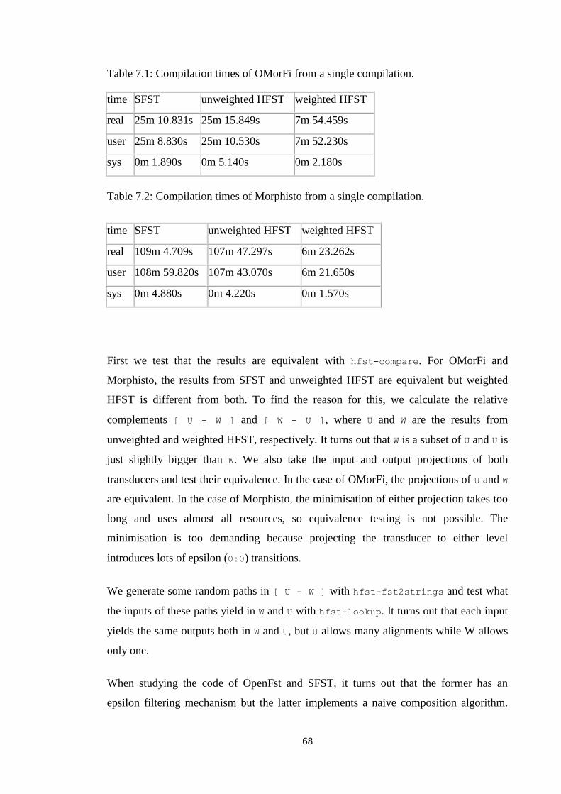
68
Table 7.1: Compilation times of OMorFi from a single compilation.
time SFST unweighted HFST weighted HFST
real 25m 10.831s 25m 15.849s 7m 54.459s
user 25m 8.830s 25m 10.530s 7m 52.230s
sys 0m 1.890s 0m 5.140s 0m 2.180s
Table 7.2: Compilation times of Morphisto from a single compilation.
time SFST unweighted HFST weighted HFST
real 109m 4.709s 107m 47.297s 6m 23.262s
user 108m 59.820s 107m 43.070s 6m 21.650s
sys 0m 4.880s 0m 4.220s 0m 1.570s
First we test that the results are equivalent with hfst-compare. For OMorFi and
Morphisto, the results from SFST and unweighted HFST are equivalent but weighted
HFST is different from both. To find the reason for this, we calculate the relative
complements [ U - W ] and [ W - U ], where U and W are the results from
unweighted and weighted HFST, respectively. It turns out that W is a subset of U and U is
just slightly bigger than W. We also take the input and output projections of both
transducers and test their equivalence. In the case of OMorFi, the projections of U and W
are equivalent. In the case of Morphisto, the minimisation of either projection takes too
long and uses almost all resources, so equivalence testing is not possible. The
minimisation is too demanding because projecting the transducer to either level
introduces lots of epsilon (0:0) transitions.
We generate some random paths in [ U - W ] with hfst-fst2strings and test what
the inputs of these paths yield in W and U with hfst-lookup. It turns out that each input
yields the same outputs both in W and U, but U allows many alignments while W allows
only one.
When studying the code of OpenFst and SFST, it turns out that the former has an
epsilon filtering mechanism but the latter implements a naive composition algorithm.
69
The naive composition algorithm does not produce false results in the case of an
unweighted transducer library, which is probably the reason why it has been left out.
The unweighted HFST seems to be slightly slower or faster than SFST. This is not
surprising because it is implemented on top of SFST and has some extra features for
symbol handling as well as some minor enhancements to the underlying SFST. The
difference in performance is so small that we are not interested in it. The system time is
negligible compared to user time, so we have no interest in listing them separately
either. We will use only unweighted and weighted HFST in our tests and show only
user time.
What is more interesting and not so predictable is that weighted HFST is much faster
than the unweighted HFST. In the case of OMorFi, weighted HFST is three and a half
times faster and in the case of Morphisto, 17 times faster. At this point it seems that
weight handling does not take extra time in OpenFst.
7.3 What explains the differences?
To see how the compilation time is divided among the OMorFi modules, each module is
compiled ten times with unweighted and weighted HFST and an average time is
calculated. Average total compilation times are calculated by summing the averages
from each module. The results are listed in table 7.3.
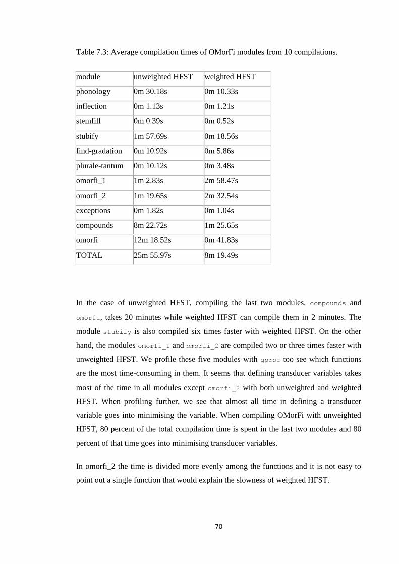
70
Table 7.3: Average compilation times of OMorFi modules from 10 compilations.
module unweighted HFST weighted HFST
phonology 0m 30.18s 0m 10.33s
inflection 0m 1.13s 0m 1.21s
stemfill 0m 0.39s 0m 0.52s
stubify 1m 57.69s 0m 18.56s
find-gradation 0m 10.92s 0m 5.86s
plurale-tantum 0m 10.12s 0m 3.48s
omorfi_1 1m 2.83s 2m 58.47s
omorfi_2 1m 19.65s 2m 32.54s
exceptions 0m 1.82s 0m 1.04s
compounds 8m 22.72s 1m 25.65s
omorfi 12m 18.52s 0m 41.83s
TOTAL 25m 55.97s 8m 19.49s
In the case of unweighted HFST, compiling the last two modules, compounds and
omorfi, takes 20 minutes while weighted HFST can compile them in 2 minutes. The
module stubify is also compiled six times faster with weighted HFST. On the other
hand, the modules omorfi_1 and omorfi_2 are compiled two or three times faster with
unweighted HFST. We profile these five modules with gprof too see which functions
are the most time-consuming in them. It seems that defining transducer variables takes
most of the time in all modules except omorfi_2 with both unweighted and weighted
HFST. When profiling further, we see that almost all time in defining a transducer
variable goes into minimising the variable. When compiling OMorFi with unweighted
HFST, 80 percent of the total compilation time is spent in the last two modules and 80
percent of that time goes into minimising transducer variables.
In omorfi_2 the time is divided more evenly among the functions and it is not easy to
point out a single function that would explain the slowness of weighted HFST.
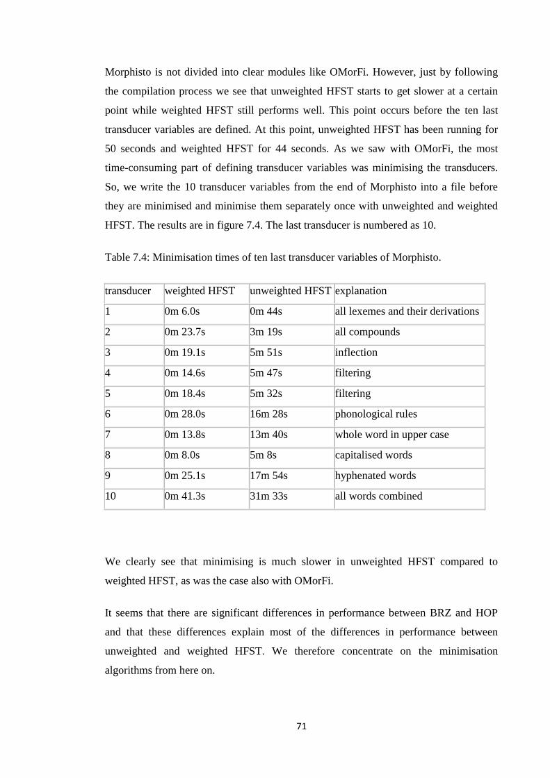
71
Morphisto is not divided into clear modules like OMorFi. However, just by following
the compilation process we see that unweighted HFST starts to get slower at a certain
point while weighted HFST still performs well. This point occurs before the ten last
transducer variables are defined. At this point, unweighted HFST has been running for
50 seconds and weighted HFST for 44 seconds. As we saw with OMorFi, the most
time-consuming part of defining transducer variables was minimising the transducers.
So, we write the 10 transducer variables from the end of Morphisto into a file before
they are minimised and minimise them separately once with unweighted and weighted
HFST. The results are in figure 7.4. The last transducer is numbered as 10.
Table 7.4: Minimisation times of ten last transducer variables of Morphisto.
transducer weighted HFST unweighted HFST explanation
1 0m 6.0s 0m 44s all lexemes and their derivations
2 0m 23.7s 3m 19s all compounds
3 0m 19.1s 5m 51s inflection
4 0m 14.6s 5m 47s filtering
5 0m 18.4s 5m 32s filtering
6 0m 28.0s 16m 28s phonological rules
7 0m 13.8s 13m 40s whole word in upper case
8 0m 8.0s 5m 8s capitalised words
9 0m 25.1s 17m 54s hyphenated words
10 0m 41.3s 31m 33s all words combined
We clearly see that minimising is much slower in unweighted HFST compared to
weighted HFST, as was the case also with OMorFi.
It seems that there are significant differences in performance between BRZ and HOP
and that these differences explain most of the differences in performance between
unweighted and weighted HFST. We therefore concentrate on the minimisation
algorithms from here on.
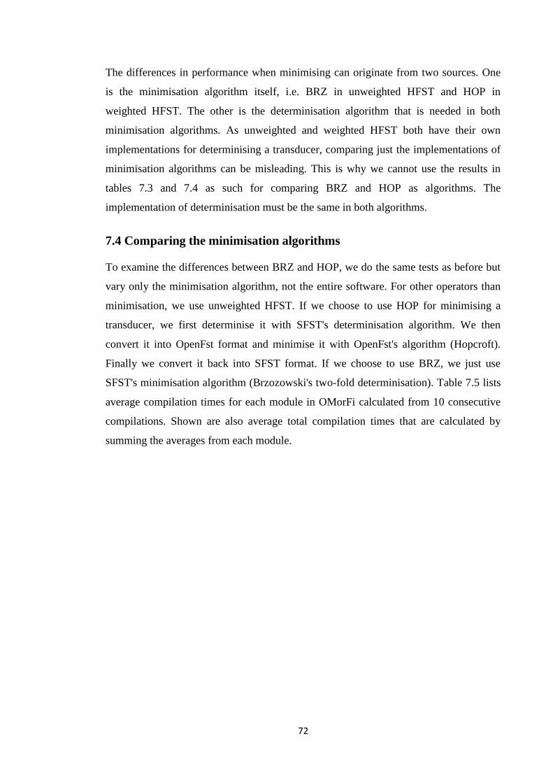
72
The differences in performance when minimising can originate from two sources. One
is the minimisation algorithm itself, i.e. BRZ in unweighted HFST and HOP in
weighted HFST. The other is the determinisation algorithm that is needed in both
minimisation algorithms. As unweighted and weighted HFST both have their own
implementations for determinising a transducer, comparing just the implementations of
minimisation algorithms can be misleading. This is why we cannot use the results in
tables 7.3 and 7.4 as such for comparing BRZ and HOP as algorithms. The
implementation of determinisation must be the same in both algorithms.
7.4 Comparing the minimisation algorithms
To examine the differences between BRZ and HOP, we do the same tests as before but
vary only the minimisation algorithm, not the entire software. For other operators than
minimisation, we use unweighted HFST. If we choose to use HOP for minimising a
transducer, we first determinise it with SFST's determinisation algorithm. We then
convert it into OpenFst format and minimise it with OpenFst's algorithm (Hopcroft).
Finally we convert it back into SFST format. If we choose to use BRZ, we just use
SFST's minimisation algorithm (Brzozowski's two-fold determinisation). Table 7.5 lists
average compilation times for each module in OMorFi calculated from 10 consecutive
compilations. Shown are also average total compilation times that are calculated by
summing the averages from each module.
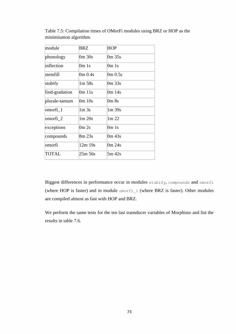
73
Table 7.5: Compilation times of OMorFi modules using BRZ or HOP as the
minimisation algorithm.
module BRZ HOP
phonology 0m 30s 0m 35s
inflection 0m 1s 0m 1s
stemfill 0m 0.4s 0m 0.5s
stubify 1m 58s 0m 33s
find-gradation 0m 11s 0m 14s
plurale-tantum 0m 10s 0m 8s
omorfi_1 1m 3s 1m 39s
omorfi_2 1m 20s 1m 22
exceptions 0m 2s 0m 1s
compounds 8m 23s 0m 43s
omorfi 12m 19s 0m 24s
TOTAL 25m 56s 5m 42s
Biggest differences in performance occur in modules stubify, compounds and omorfi
(where HOP is faster) and in module omorfi_1 (where BRZ is faster). Other modules
are compiled almost as fast with HOP and BRZ.
We perform the same tests for the ten last transducer variables of Morphisto and list the
results in table 7.6.
74
Table 7.6: Compilation times of the ten last transducer variables of Morphisto using
BRZ or HOP as the minimisation algorithm.
transducer BRZ HOP
1 0m 45s 0m 6s
2 3m 22s 0m 24s
3 6m 4s 0m 19s
4 6m 2s 0m 15s
5 5m 43s 0m 22s
6 16m 25s 0m 36s
7 13m 37s 0m 13s
8 5m 7s 0m 8s
9 17m 54s 0m 26s
10 31m 24s 0m 39s
TOTAL 105m 44s 3m 28s
It seems again that minimising with BRZ is much slower than with HOP.
7.5 What explains the differences in HOP and BRZ?
Now we have established the major factor that explains the difference in performance
between unweighted and weighted HFST, i.e. the minimisation algorithms. We have
also found where this difference in performance occurs. At this point, we are interested
in (1) what kind of transducers are slower to minimise with BRZ or HOP and (2) what
happens in the minimisation process.
The only OMorFi module that is clearly faster to compile with BRZ is omorfi_1. It
contains some 150 gradation replace rules that are applied to a lexical acyclic transducer
one rule at a time. The rules are ready compiled in modules phonology and
find-gradation.
The OMorFi modules that are faster to compile using HOP are stubify, compounds
and omorfi. stubify contains 153 (cyclic) replace rules that are all composed into a
single rule. compounds constructs compound words from the lexical transducers
75
omorfi_1 and omorfi_2, something like [ (omorfi_1 | omorfi_2) + ] in
simplified form. omorfi disjuncts modules compounds, exceptions, omorfi_1 and
omorfi_2 One difference between these slow modules and omorfi_1 is that the
previous ones are all cyclic but the latter is acyclic. On the other hand, module
phonology is cyclic but slightly faster to compile using BRZ. However, the transducers
in this module are very small compared to stubify, compounds or omorfi.
The point in Morphisto where compilation gets slower with BRZ is very similar to the
OMorFI module compounds. There a cyclic suffix transducer is appended to a lexical
acyclic transducer and a plus operator is applied to the concatenation, something like
[ ( LEXICON SUFFIX ) + ] in simplified form.
These observations lead to our initial hypothesis: Big cyclic transducers are faster to
minimise with HOP, acyclic lexical transducers are sometimes faster with BRZ.
Since the biggest differences in performance originate from cases where BRZ is slower
than HOP, we will focus on them. We will first see what happens in minimisations and
then test our hypothesis. Since the slowest minimisations in OMorFi occur at the end of
modules compounds and omorfi, we will write the two last transducer variables from
each module to file and minimise them separately, as we did in Morphisto. This allows
us to see in more detail what happens in the minimisation of a single transducer.
7.6 What happens in minimisation?
We write the ten last transducer variables of Morphisto and the two last transducer
variables of compounds and omorfi into file and minimise them. For each transducer,
we calculate their number of states and arcs initially, after plain determinisation (in
HOP), after backward determinisation (BD) of BRZ and finally (after HOP or BRZ). In
table 7.7, we present the same numbers so that instead of their absolute value, they are
divided by the number of words or arcs in the initial transducer. This allows us to see
more clearly if the number of states/arcs increases or decreases in the intermediate
transducers. Since it seems that BRZ is much slower than HOP, the percentage of time
spent in BD and in forward determinisation (FD) in BRZ is also shown. The last
transducers in OMorFi modules are numbered as 2 and in Morphisto as 10.
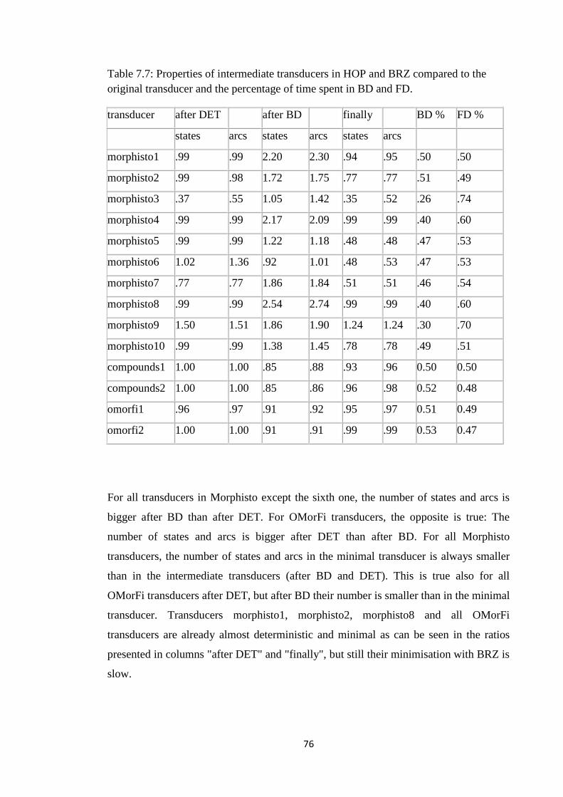
76
Table 7.7: Properties of intermediate transducers in HOP and BRZ compared to the
original transducer and the percentage of time spent in BD and FD.
transducer after DET after BD finally BD % FD %
states arcs states arcs states arcs
morphisto1 .99 .99 2.20 2.30 .94 .95 .50 .50
morphisto2 .99 .98 1.72 1.75 .77 .77 .51 .49
morphisto3 .37 .55 1.05 1.42 .35 .52 .26 .74
morphisto4 .99 .99 2.17 2.09 .99 .99 .40 .60
morphisto5 .99 .99 1.22 1.18 .48 .48 .47 .53
morphisto6 1.02 1.36 .92 1.01 .48 .53 .47 .53
morphisto7 .77 .77 1.86 1.84 .51 .51 .46 .54
morphisto8 .99 .99 2.54 2.74 .99 .99 .40 .60
morphisto9 1.50 1.51 1.86 1.90 1.24 1.24 .30 .70
morphisto10 .99 .99 1.38 1.45 .78 .78 .49 .51
compounds1 1.00 1.00 .85 .88 .93 .96 0.50 0.50
compounds2 1.00 1.00 .85 .86 .96 .98 0.52 0.48
omorfi1 .96 .97 .91 .92 .95 .97 0.51 0.49
omorfi2 1.00 1.00 .91 .91 .99 .99 0.53 0.47
For all transducers in Morphisto except the sixth one, the number of states and arcs is
bigger after BD than after DET. For OMorFi transducers, the opposite is true: The
number of states and arcs is bigger after DET than after BD. For all Morphisto
transducers, the number of states and arcs in the minimal transducer is always smaller
than in the intermediate transducers (after BD and DET). This is true also for all
OMorFi transducers after DET, but after BD their number is smaller than in the minimal
transducer. Transducers morphisto1, morphisto2, morphisto8 and all OMorFi
transducers are already almost deterministic and minimal as can be seen in the ratios
presented in columns "after DET" and "finally", but still their minimisation with BRZ is
slow.
77
Sometimes the BD takes more time than the FD, but in many cases the time is divided
equally between the determinisations. The amount of time spent in BD and FD does not
clearly correlate with the increase/decrease in the size of the transducers after BD/DET.
Although determinisation in HOP (DET) and the second determinisation in BRZ (FD)
effectively do the same thing, it is much slower in the latter case. While BD decreases
the multiplicity in backward direction to 1, it probably increases the multiplicity in the
forward direction, since FD would else take equally long as DET.
The increase in the size of the transducer after BD could explain the slowness of BRZ in
the cases where it occurs. However, BRZ is slow even in cases where the size of the
transducer decreases after BD.
Next we test out previous hypothesis with Kotus's wordlist.
7.7 Testing the cyclicity hypothesis
The word list of Kotus contains little over 90 000 lexemes (many of which are
compounds) in alphabetical order. We take N of these lexemes and disjunct them all and
get a lexical transducer [ LEX ]. The number of lexemes, N, can be 10 000, 20 000, ...
80 000 or 90 000. The lexemes are chosen evenly; e.g. instead of taking 10 000 first
words we take every 9th word from the 90 000 first words. As a result we get nine
lexical transducers that recognise a set of 10, 20, 30 ... and 90 thousand Finnish words
in their base form.
We also create two transducers that recognise simple compounds, i.e. [ LEX* ] and
[ LEX+ ]. The former transducer does not actually work correctly as it recognises also
the empty string, but we include it in our tests to see if the minimisation algorithms
perform differenty on it compared to the latter transducer. It is evident that we greatly
simplify the compound mechanism when we take all words in the list and allow them to
combine in any order. However, our aim is to obtain information on how cyclicity
affects the performance of HOP and BRZ in general. We will not use the word list of
Morphisto because it has only 18624 words.
Since many test transducers in section 7.6 were already almost deterministic and
minimal, we minimise all our test transducers before minimisation tests. This makes it

78
easier to see what happens to the properties (number of states and arcs) of the transducer
in the minimisation.
Next we minimise transducers [ LEX ], [ LEX+ ] and [ LEX* ] with HOP and BRZ
and plot the minimisation times as a function of the number of states in the transducer.
We perform every minimisation ten times and calculate an average. The results are in
figures 7.1-3.
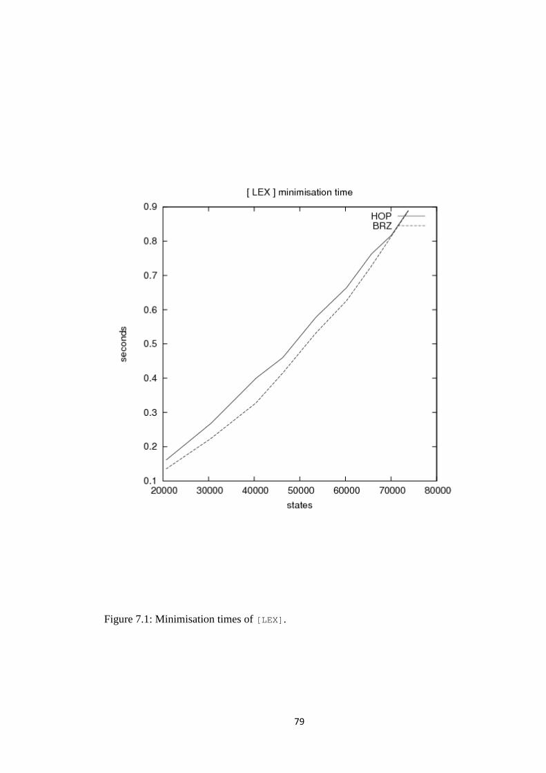
79
Figure 7.1: Minimisation times of [LEX].
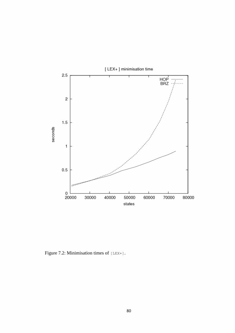
80
Figure 7.2: Minimisation times of [LEX+].

81
Figure 7.3: Minimisation times of [LEX*].
82
We see that in the case of a lexical transducer [ LEX ], BRZ is slightly faster that HOP
and the minimisation time increases fairly linearly with both algorithms as the number
of states increases. In the case of compound transducers [ LEX* ] and [ LEX+ ], HOP
clearly outperforms BRZ on big transducers. The time in HOP still grows linearly,
while the time in BRZ seems to increase almost polynomially. BRZ is slightly faster
when the number of states is lower than 40 000 in [ LEX* ] and lower than 30 000 in
[ LEX+ ].
It is not evident how BRZ will behave in [ LEX ] when the number of states increases
over 70 000. The BRZ line is somewhat curved which might suggest that the growth is
actually polynomial, but it is not clearly visible on smaller transducers.
83
8. Discussion
In the first section, we summarise the results from the tests. In the second section, we
compare the results with literature. In the third section, we some report some
observations made during the tests that could be studied further.
8.1 The results from the tests summarised
In our tests, we compiled OMorFi and Morphisto with SFST, unweighted HFST and
weighted HFST. We found out that weighted HFST is faster than unweighted HFST.
When profiling further, we saw that this difference is due to different minimisation
algorithms in the underlying finite-state libraries, OpenFst in weighted HFST and SFST
in unweighted HFST. OpenFst uses Hopcroft's minimisation algorithm and SFST
Brzozowski's.
By comparing the cases where HOP was faster to the cases where BRZ was faster we
discovered that HOP is much faster on large transducers that have large-scale cyclicity,
i.e. have cycles that lead from the nearness of the final states to the nearness of initial
states. We examined the properties of the intermediate transducers in HOP and BRZ to
find a reason to the slowness of BRZ. It turned out that in many cases the number of
states and arcs after backwards determinisation was substantially bigger than in the
original or minimal transducer. On the other hand, some transducers had less or almost
an equal number of states and arcs after BD. In HOP, the number of states and arcs after
DET was usually smaller than in the original transducer, although there were some
opposite cases.
To examine the reason for the slowness of BRZ on cyclic transducers, we performed a
series of tests on simple test transducers that consisted only of base form lexemes. We
found out that BRZ and HOP perform equally on acyclic transducers and the time that
they take grows linearly with the number of states in the transducer. The algorithms also
perform equally on cyclic transducers that have less than 30 000 or 40 000 states, but
when the number of states increases, the time grows exponentially if BRZ is used and
linearly if HOP is used.
84
8.2 Comparisons with literature
Brzozowski's minimisation algorithm is often said to perform well in practice (see
references in section 4.3.4). We found out that this is not always the case. With
morphologies that have compound mechanisms, such as Finnish or German, it can be
substantially slower than Hopcroft's minimisation algorithm. No clear reason for its
slowness was found, but some observations were made. It seems that large transducers
that have large-scale cyclicity can be tens of times slower to minimise with BRZ than
with HOP. In most acyclic cases BRZ performs well, sometimes even slightly
outperforming HOP. However, its slowness in cyclic transducers makes it a bad choice
for a morphology that has a compound mechanism.
The performance of BRZ has not been tested on real linguistic data before. However, a
quite recent thesis by Måns Huldén (2009) includes a chapter where different
minimisation algorithms are compared. In his tests, he compares different
implementations of HOP, including his own, with BRZ on finite-state morphologies. It
turns out that many implementations of HOP often need more time to minimise a
transducer than BRZ. However, his own efficient implementation of HOP clearly
outperforms BRZ on all morphologies that are included in his tests. Huldén thus offers
an explanation for the widespread notion that BRZ is equally fast as HOP or even faster,
stating that HOP is underestimated because it is often poorly implemented. Another
reason for BRZ being cited as an efficient minimisation algorithm could be that many
FSMs have been done for English whose compound mechanism is much simpler than
that of Finnish or German.
8.3 Future work
Our tests showed that HOP was faster than BRZ both in the case of OMorFi and
Morphisto. BRZ got slower at the point where large-scale cyclicity (due to
compounding mechanism) was introduced to the transducers. The same behaviour was
observed on simple lexical test transducers if they were made cyclic by applying a star
or plus operator (simulating a very naive compounding mechanism).
However, we found no clear explanation for this phenomenon. We observed that the
number of states and arcs grew in many cases after BD, but there were also cases where
85
the size of the transducer was almost the same before and after BD. The growth in the
size of the transducer clearly cannot be the only reason for the slowness of BRZ.
The slowness of BRZ was observed in the simple test transducers when the number of
states was 30 000 - 40 000 or higher. It is possible that the test transducers were too
simple and did not model the compounding mechanism of OMorFi or Morphisto well
enough. Nevertheless, they offered some support for the hypothesis of cyclicity making
BRZ slow.
We made some efforts to find a reason to the slowness of BRZ on cyclic transducers.
For OMorFi and Morphisto, we followed the following strategy: We wrote the
intermediate transducer in file at the point where BRZ got slow and minimised it
separately with HOP and BRZ. We timed both algorithms and calculated the properties
(the number of states and arcs and the number of final states) at different points of the
algorithms, i.e. after DET, BD and FD. The intermediate transducers that we minimised
were a result of a lexicon transducer and a set of (compounding) rule transducers.
Accordingly, we also varied the number of rules applied to the lexicon as well as the
number of words taken from the word list to the lexicon transducers. We also varied the
way in which the words were taken from the list: either N first words or every Nth
word.
We did many tests and draw many graphs and transducers with dotty. However, we
needed to take hundreds of words to see even a slight difference either in the times of
the algorithms or in the properties of the transducers in the intermediate stages of the
algorithms. Actually, thousands of words were needed to get a clearly visible difference.
Thousand words is of course a much smaller number than the 30 000 - 40 000 words
that were needed in our simple test transducers to get BRZ slower than HOP. However,
a thousand-word transducer still has hundreds of states and arcs. It is very difficult to
see in a graph of a transducer where the extra states or arcs occur or where the slowness
could originate from.
The slowness of BRZ is a complicated equation. Rules and words interact in some way,
and to find out which rules and words interact in which ways is very challenging. It is
difficult to choose a smallest sufficient number of rules and words to get clearly visible
differences between HOP and BRZ.

86
One reason for the slowness of BRZ can be the subset construction. The size of the
transducer can remain almost the same after determinisation although the subsets that
constitute a state in the DFA get big. How the size of subsets varies in the
determinisation phases (BD and FD) and what kind of linguistic properties can cause
big subsets are questions worth studying.
87
9. Conclusions
We compiled two finite-state morphologies, OMorFi for Finnish and Morphisto for
German, using the HFST transducer library with unweighted and weighted mode. The
unweighted mode of operation is based on SFST and the weighted one on OpenFst.
OMorFi was compiled in 25 minutes with unweighted HFST and in 8 minutes with
weighted HFST. Morphisto was compiled in 109 minutes with unweighted HFST and in
less than 6 and a half minutes with weighted HFST. The major factor explaining the
difference in performance was the minimisation algorithm, Brzozowski's in SFST and
Hopcroft's in OpenFst. For individual modules in the FSMs, HOP was in some cases 50
times faster than BRZ.
The slowness of BRZ was evident in transducers that contained large-scale cyclicity, i.e.
had transitions leading from the nearness of the final states to the nearness of initial
states. These kinds of transducers often occur in FSMs that have a compounding
mechanism. No clear reason was found for this behaviour, but in many cases the
number of states and arcs after backwards determinisation in BRZ was substantially
bigger than in the original or minimal transducer.
Contrary to claims in the literature, BRZ turned out to be much slower than HOP.
Reasons for this misconception can be: (1) Many FSMs are implemented for English
language that has a simple compounding mechanism, unlike Finnish and German. (2)
The minimisation algorithms have not been benchmarked on real linguistic data before.
(3) The minimisation algorithms are poorly implemented and therefore HOP seems to
be much slower (Huldén, 2009).
If a choice must be made between HOP and BRZ, the previous is a better choice for a
minimisation algorithm. BRZ is sometimes faster than HOP, but in that case their
difference is quite small. In the cases where BRZ is slower than HOP, their difference is
much bigger, BRZ sometimes being 50 times slower than HOP. Of course, BRZ is
much easier to implement since it uses two basic operations, determinisation and
reversion.
At least the developers of free-source transducer libraries can use OpenFst's
minimisation algorithm if the implementation of HOP is considered too demanding a
88
task. The transducers can be converted to OpenFst format (via AT&T table format),
minimised with OpenFst and converted back to the original format. This is exactly what
was done in section 7.4. This solution will probably be used in future versions of HFST,
too. If the user chooses to use unweighted transducers, the SFST library is used but
minimisations are done with OpenFst's minimisation algorithm.
89
List of references
Aho, Alfred V. & Ullman, Jeffrey D., 1978. Principles of Compiler Design. 2nd
printing. USA: Addison-Wesley. (Aho & Ullman, 1978)
Almeida, A., Moreira, N. & Reis, Rogério, 2007. On the performance of
automata minimization algorithms. Technical report, Universidade do Porto.
(Almeida et al., 2007)
Beesley, Kenneth R. & Karttunen, Lauri, 2003. Finite State Morphology. USA:
CSLI Publications. (Beesley & Karttunen, 2003)
Castiglione, Giusi, Restivo, Antonio & Sciortino, Marinella, 2008. Hopcroft’s
Algorithm and Cyclic Automata. Lecture Notes in Computer Science, 5196, pp.
172–183. (Castiglione et al., 2008)
Champarnaud, J.-M., Khorsi, A. & Paranthoën, T., 2002. Split and join for
minimising: Brzozowski's algorithm. In Proceedings of PSC 2002 (Prague
Stringology Conference). (Champarnaud et al., 2002)
Hopcroft, John E., Motwani, Rajeew, & Ullman, Jeffrey D., 2001. Introduction
to Automata Theory, Languages, and Computation. 2nd ed. USA: Addison-
Wesley. (Hopcroft et al., 2001)
Huldén, Måns, 2009. Finite-state machine construction methods and algorithms
for phonology and morphology. Ph. D. The University of Arizona. (Huldén,
2009)
Karlsson, Fred, 2004. Yleinen kielitiede. 2nd ed. Helsinki University Press.
(Karlsson, 2004)
Koskenniemi, Kimmo, 1983. Two-Level Morphology: A general computational
Model for Word-Form Recognition and Production. Ph. D. University of
Helsinki. (Koskenniemi, 1983)
Koskenniemi, Kimmo, 1996. Finite-state morphology and information retrieval.
Proceedings of the ECAI 96 Workshop. (Koskenniemi, 1996)
Pereira, Fernando C. N. & Riley, Michael D., 1997. Speech Recognition by
Composition of Weighted Finite Automata. In: Roche, E. and Schabes, Y.,
Finite-State Language Processing, MIT Press, Cambridge, MA, pp. 431-453.
(Pereira & Riley, 1997)
Pirinen, Tommi, 2008. Suomen kielen äärellistilainen automaattinen
morfologinen analyysi avoimen lähdekoodin menetelmin. Master's thesis.
90
University of Helsinki. (available from http://www.helsinki.fi/~tapirine/gradu/)
(Pirinen, 2008)
Schmid, Helmut, ?, SFST Manual. (available from
ftp://ftp.ims.uni-stuttgart.de/pub/corpora/SFST/SFST-Manual.pdf) (Schmid)
Tabakov, Deian & Vardi, Moshe Y., 2005. Experimental Evaluation of Classical
Automata Constructions. 12th International Conference on Logic for
Programming, Artificial Intelligence and Reasoning. (Tabakov & Vardi, 2005)
Watson, Bruce W., 1995. Taxonomies and Toolkits of Regular Language
Algorithms. Ph. D. Eindhoven University of Technology. (Watson, 1995)
Internet resources:
HFST home page. http://hfst.sourceforge.net/
OMorFi code. http://kitwiki.csc.fi/twiki/bin/view/KitWiki/OMorFiSFSTVersion
Morphisto code. http://code.google.com/p/morphisto/
SFST home page.
http://www.ims.uni-stuttgart.de/projekte/gramotron/SOFTWARE/SFST.html
OpenFst home page. http://www.openfst.org/


