Analysis of cycle stealing with switching cost

Analysis of Cycle Stealing with Switching Cost

Takayuki Osogami�

Mor Harchol-Balter�

Alan Scheller-Wolf�

October 2002

CMU-CS-02-192

School of Computer Science

Carnegie Mellon University

Pittsburgh, PA 15213

Abstract

We consider the scenario of two independent processors, each serving its own workload, where one of theprocessors (known as the “donor”) can help the other processor (known as the “beneficiary”) with its jobs,during times when the donor processor is idle. That is the beneficiary processor “steals idle cycles” fromthe donor processor. We assume that both donor jobs and beneficiary jobs may have generally-distributedservice requirements. We assume that there is a switching cost required for the donor processor to startworking on the beneficiary jobs, as well as a switching cost required for the donor processor to returnto working on its own jobs. We also allow for threshold constraints, whereby the donor processor onlyinitiates helping the beneficiary if both the donor is idle and the number of jobs at the beneficiary exceedsa certain threshold.We analyze the mean response time for the donor and beneficiary processors. Our analysis is approxi-mate, but can be made as close to exact as desired. Analysis is validated via simulation. Results of theanalysis illuminate several interesting principles with respect to the general benefits of cycle stealing andthe design of cycle stealing policies.

�

Carnegie Mellon University, CSD. Email: [email protected]�

Carnegie Mellon University, Computer Science Department. Email: [email protected]. This work was supported byNSF Career Grant CCR-0133077, by NSF ITR Grant 99-167 ANI-0081396 and by Spinnaker Networks via Pittsburgh DigitalGreenhouse Grant 01-1.

�

Carnegie Mellon University, GSIA. Email: [email protected]

Keywords: cycle stealing, switching cost, queueing theory, task assignment, server farm, distributed

system, unfairness, starvation, load sharing, supercomputing, Matrix-Analytic.

1 Introduction

Motivation

Since the invention of networks of workstations, systems designers have touted the benefits of allowing

a user to take advantage of machines other than her own, at times when those machines are idle. This

notion is often referred to as cycle stealing. Cycle stealing allows a user, Betty, with multiple jobs to

offload one of her jobs to Dan’s machine if Dan’s machine is idle, giving Betty two machines to process

her jobs. When Dan’s workload resumes, Betty must return to using only her own machine. We refer to

Betty as the beneficiary, to her machine as the beneficiary machine/server, and to her jobs as beneficiary

jobs. Likewise, we refer to Dan as the donor, to his machine as the donor machine/server, and to his jobs

as donor jobs.

Although cycle stealing provides obvious benefits to the beneficiary, these benefits come at some cost

to the donor. For example, the beneficiary’s job may have to be checkpointed and the donor’s working

set memory reloaded before the donor can resume, delaying the resumption of processing of donor jobs.

In our model we refer to these additional costs associated with cycle stealing as switching costs.

A primary goal of this paper is to understand what is the benefit of cycle stealing for the beneficiary

and what is the penalty to the donor, as a function of switching costs. A second goal is to derive parameter

settings for cycle stealing. In particular, given non-zero switching costs, cycle stealing may only pay if the

beneficiary’s queue is “sufficiently” long. We seek to understand the optimal threshold on the beneficiary

queue. More broadly, we seek general insights into which problem parameters have the most significant

impact on the effectiveness of cycle stealing.

The analytical model

We assume two independent M/GI/1/FCFS queues, the beneficiary queue and the donor queue. Jobs

arrive at rate��

(respectively,��

) at the beneficiary (respectively, donor) queue and have service re-

quirement represented by the random variable � � drawn from distribution � � (respectively, � � drawn

from distribution � � ). The load made up by beneficiary (respectively, donor) jobs is denoted by � �

(respectively, � � ) where � �� and � �� . If the donor server is idle, and if

the number of jobs at the beneficiary queue is at least �� , the donor transitions into the switching state,

for a random amount of time, �� . After �� time, the donor server is available to work on the bene-

ficiary queue and the beneficiary queue becomes an M/ � � /2 queue. If a donor job arrives during �� ,

or during the time the donor is helping the beneficiary, the donor transitions into a switching back state,

for a random amount of time, �! #" . After the completion of the switch back, the donor server resumes

working on its own jobs. We assume the first four moments of the service times are finite, and queues

1

are stable. No work is accomplished by the donor server while switching.

A few details are in order. First, in the above model, the donor processor continues to cooperate with

the beneficiary even if there is no beneficiary work left for it to do — the donor processor only switches

back when a donor job arrives. (We also analyzed the case where the donor processor switches back when

it is not needed, see Appendix A. We found that this has almost no effect on performance, even under

high switching costs). Second, we assume that if the donor processor is working on a beneficiary job and

a donor job arrives, that beneficiary job is returned to the beneficiary queue and will be resumed by the

beneficiary processor as soon as that processor is available. The work done on the job is not lost, i.e., the

job is checkpointed.�

Finally, our model can be generalized to the case where there is a threshold, � �� ,

on the number of donor jobs as well — i.e., the donor processor only returns to the donor queue when

the number of jobs at the donor queue is at least � �� . Throughout this paper, aside from the stability

section (Section 4), we assume � �� for simplicity, and focus on the effect of � �� . In Appendix B,

we extend the analysis to general � �� . Our performance metric throughout is mean response time for

each class of jobs.

Difficulty of analysis and Previous work

Consider the simplest instance of our problem — where the service requirements of all jobs are each

drawn from exponential distributions and the switching costs and threshold are zero. Even for this sim-

plest instance the continuous-time Markov chain, while easy to describe, is mathematically intractable.

This is due to the fact that the stochastic process having state (number beneficiary jobs, number donor

jobs ) grows infinitely in two dimensions and contains no structure that can be exploited to obtain an ex-

act solution. While solution by truncation of the Markov chain is possible, the errors that are introduced

by ignoring portions of the state space (infinite in two dimensions) can be quite significant, especially at

higher traffic intensities.�

Thus truncation is neither sufficiently accurate nor robust for our purposes.

To our knowledge, there has been no previous analytical work on the problem of cycle stealing

with setup costs. Below we describe prior work on the “coupled processor model”. In this model two

processors each serve their own class of job, and if either is idle it may help the other, increasing the

rate of this other processor. This help incurs no switching cost and has an effect if even a single job is

present. These models inherently assume a preemptive resume discipline: when a processor returns to

�

It is easy to generalize our analysis to the case where the beneficiary requires a “switching time” before it can resume a jobthat the donor started. We have chosen to ignore this generalization for purpose of clarity. It is also trivial to extend our resultsto the case where all work on the job in progress is lost if a donor job arrives, provided that we assume that the job is restartedwith a new service time – which we feel is unrealistic. It is also possible to extend our results to the case where the donor mustcomplete the beneficiary job in progress before it switches back. This is the topic of current research, see Section 7.

�

For �� and �� , truncation leads to �� error, even with ��

states, and takes �� minutes to compute.As �� nears �� , the error increases indefinitely. Under jobs sizes more variable than exponential, the error increases.

2

its own queue, none of its work is lost. All works we mention below consider Poisson arrivals.

Early work on the coupled processor model was by Fayolle and Iasnogorodski [5] and Konheim,

Meilijson and Melkman [6]. Both papers assume exponential service times, deriving expressions for

the stationary distribution of the number of jobs of each type. Fayolle and Iasnogorodski use complex

algebra, eventually solving either a Dirichlet problem or a homogeneous Riemann-Hilbert problem for a

circle, depending on the accelerated rates of the servers. Konheim et. al. assume that the accelerated rate

is twice the original rate, which yields simpler expressions (still in the form of complex integrals). No

indication is given in either work as to how the evaluation of these expressions. In addition, because the

processors work in concert, rather than on different jobs, these systems will gain no multi-server benefit

when serving highly variable jobs; short jobs may get stuck waiting behind long jobs in a single queue.

The above work was extended by Cohen and Boxma [4] to the case of general service times. They

consider stationary workload, which they formulate as a Wiener-Hopf boundary problem. This leads

to complex expressions involving either integrals or infinite sums; if the queues are symmetric simpler

expressions for mean total workload are found. They again have the two processors working in concert,

without a switching cost, providing complex analytical expressions, rather than numerical values.

In more recent work, Borst, Boxma and van Uitert [3] apply a transform method to the expressions in

[4], yielding asymptotic relations between the workloads and the service requirement distributions. This

leads to the insight that if a processor has a load less than one, it is “insulated” from the heavy-tail of the

other, as long periods without cooperation will not lead to large backlogs. This is not the case if the load

is greater than one, as the queue now must rely on help to be stable. Borst, Boxma and Jelenkovic [2]

consider a very similar question under generalized processor sharing. Using probabilistic bounds, they

show that different service rates can either insulate the performance of different classes from the others

or not, again depending on whether the minimal rate is larger than the load. Both of these papers are

concerned with the asymptotic behavior of workload, whereas our work isolates mean performance. Our

work is thus complementary to these results.

Our approach

This paper presents the first analysis of cycle stealing under general service requirements with switching

costs and a switching threshold. Recall that the difficulty in analyzing cycle stealing is that the cor-

responding stochastic process defines a Markov chain which grows infinitely in two dimensions (2D),

making it intractable. The key idea in our approach is to find a way to transform this 2D chain into some

1D infinite Markov chain which can be analyzed. The questions in applying such a transformation are

(i) what should the 1D Markov chain track, and (ii) how can all the relevant information from the 2D

chain be captured in the 1D chain. Our 1D chain tracks the number of beneficiary jobs. For the donor

3

jobs, our state space contains only binary knowledge: zero jobs or � �jobs. Nevertheless we are able

to capture detailed information on the number of donor jobs by using special transitions in our Markov

chain, where these transitions represent the lengths of an assortment of busy periods. The difficulty lies

in specifying the right busy periods, some of which transcend the definition of the analytical model.

Once the 1D Markov chain is specified, the hard work is finished, since this chain can be solved

efficiently using known numerical (Matrix analytic) techniques. While a closed-form solution may be

preferable, our chain is compact enough, and Matrix analytic methods powerful enough, that only a

couple seconds are required to generate any of the results plots in this paper. Furthermore, our method

very easily generalizes to more complex problem formulations e.g., multiple donors (Section 7).

Our analysis is approximate, but can be made as close to exact as desired. The only approximation

lies in representing the length of the busy periods by a Coxian distribution fit to a finite number of the

busy period moments. In this paper, we use a 2-stage Coxian to capture the first 3 moments of the

busy periods, and verify that this is sufficient via simulation. However, our method naturally extends to

matching more moments.

Our analysis assumes a Poisson arrival process for both classes of jobs. The service requirements

of the each class are assumed to be drawn i.i.d. from general distributions (which we approximate by a

Coxians). The arrival process can easily be generalized to a MAP – Markovian Arrival Process [1].

Summary of results

Our analysis yields many interesting results concerning cycle stealing, detailed in Section 6. While

cycle stealing obviously benefits the beneficiaries and hurts the donors, we find that when � �� ,

cycle stealing is profitable overall even under significant switching costs as it may ensure stability of

the beneficiary queue. For � �� , we define load-regions under which cycle stealing pays. We find

that in general the switching cost is only prohibitive when it is large compared with�� . Under zero

switching cost, cycle stealing always pays.

Two counterintuitive results are that when � �� , the performance of the beneficiaries is sur-

prisingly insensitive to the switching cost, and also insensitive to the variability of the donor job size

distribution. Even when the variability of the donor job sizes is very high, and donor help is very bursty,

the beneficiaries don’t seem to suffer.

We also study the effect of � �� , and present several rules of thumb for choosing the optimal setting

of � �� as a function of the server loads, the switching cost, and the mean job sizes.

4

Outline

In Section 2 we present our analysis for the case of zero switching cost, generalizing to non-zero cost in

Section 3. In Section 4 we provide stability conditions for the donor and beneficiary hosts. In Section 5

we validate our analysis by considering limiting analytical cases and via simulation. In Section 6 we

present results for mean response times of donor and beneficiary jobs under various loads, job size

distributions, switching costs, and thresholds. Section 7 describes extensions to the model.

2 Analysis without switching cost

In this section we analyze the simpler case of zero switching cost. Figure 1 shows our Markov chain

for the case where � �� , i.e. the donor server switches to help beneficiary jobs when there are zero

donor jobs and there are at least three beneficiary jobs. Figure 1(a) shows a simplified form of our chain

where job sizes and busy periods are assumed to be exponentially-distributed. Figure 1(b) and (c) show

the case of generally-distributed (Coxian) job sizes and busy periods. The actual chain that we evaluate

in the paper is a superposition of the chains in Figure 1(b) and (c), shown in Appendix C.

The first two components of each state denote the number of beneficiary jobs and the number of

donor jobs respectively. The states of the Markov chain have been grouped into three rows, labeled (i)

cooperating row: indicates that the donor processor is cooperating with the beneficiary; (ii) independent

row, with � � donor job: indicates that the donor and beneficiary processors are each working indepen-

dently on their own queues and there is at least 1 donor job present; (iii) independent row, with � donor

jobs: indicates that the donor and beneficiary processors are each working independently on their own

queues and there are zero donor jobs present.

Observe that while the states track the precise number of beneficiary jobs, they keep only a binary

record (zero or � � ) of the donor jobs. The key idea is that to determine beneficiary performance we can

avoid tracking the number of donor jobs because we only need to know when the donor queue is idle.

Thus we use transitions (labeled � � ) to represent the length of a busy period of donor jobs.

The logic behind the Markov chain in Figure 1(a) is as follows: If we are in the row where the

processors are working independently and the number of donor jobs is zero, the left-right transitions

allow us to track the number of beneficiary jobs. If a donor job arrives we transition to the row where

processors are working independently and the number of donor jobs is at least one. The time spent in this

row is the length of a donor busy period. If at the end of the busy period the number of beneficiary jobs

is below � �� , then we return to the row where processors are working independently and the number of

donor jobs is zero. If however at the end of the busy period the number of beneficiary jobs is at least

� �� , then we move to the cooperating row, where we stay until there is a donor arrival.

5

WorkingIndependently,# Donors = 1+

WorkingIndependently,# Donors = 0

λB

µB

2

λB

µB

2

λB

µB

2

λB

µB

2B,0D,C1B,0D,C0B,0D,C 4B,0D,C3B,0D,C

λD BDλD

λD λD BDλD

λB

λB

µB

µB

µB

λB

λB

λB

µB

λB

µB

Dλ BDλD BD BD

λD

µB

λB

CooperatingServers

1B,0D0B,0D 2B,0D

0B,1D 1B,1D 2B,1D 3B,1D 4B,1D

(a)

λB

λB

µB

λB

µB

µB

λB

λB

λB

µB

µB

λB

µB

µB

λB

λB

µB

λD

λD

λD

λD λ

Dλ

D

λD

λD β3

λB

µB

2

λB

µB

2

λB

µB

2

λB

µB

2B,0D,C1B,0D,C0B,0D,C 4B,0D,C3B,0D,C

β1β1β1β2 β2 β2

β2β2

β3 β3 β3

β1λB

µB

λB

µB

β3

β1

1B,0D0B,0D 2B,0D

0B,1D 1B,1D 2B,1D 3B,1D 4B,1D

(b)

b2

b3

2b22b22b2

b3

b2

b1

b3

b2

b1

b3

b3

b3b1

b3

b1

b2 b2

b1

2b1b3

2b3

b2

b1

2b12b3

b2

b3

b1b3

b2

2b3

b2

λB

λDb2

b3b1XB

ΒD

b1

b2

b3b3 b3

2b1b1 b3

b1

2B,0D,C1B,0D,C0B,0D,C

1B,0D0B,0D 2B,0D

4B,0D,C3B,0D,C

4B,1D3B,1D2B,1D1B,1D0B,1D

(c)

Figure 1: Markov chain for cycle stealing without switching cost. (a) Where � � is exponential and � �is drawn using a single (exponential) transition. (b) Where � � is exponential, and � � is representedby a 2-stage Coxian. (c) Where � � is represented by a 2-stage Coxian and � � is drawn using a single(exponential) transition.

6

Figure 1(b) and (c) show the same Markov chain as 1(a), where now � � and � � are represented

by 2-stage Coxian distributions. Observe that when the donor and beneficiary are cooperating, the state

space now must maintain a state for two partially-completed beneficiary jobs. If a donor job arrives while

we’re in the cooperating row, the partially-completed job that the donor was working on will be moved

to the head of the beneficiary queue (we currently assume zero cost for the transfer, but this is easy to

generalize to non-zero cost).

In order to specify the Markov chain, we need to compute the first three moments of � � and then

find a 2-stage Coxian which matches these. The Laplace transform of ��

is:

��

��

The moments of � � are obtained from the transform by taking derivatives. In [9] we derive necessary

and sufficient condition for matching the first three moments of a distribution using a 2-stage Coxian.

2.1 Computing response times

The mean response time for donor jobs is trivial to compute – it is simply the response time of the

M/ � � /1 queue, since the beneficiary jobs are preemptive and switching cost is zero.

The mean number of beneficiary jobs is easy to compute from the chain in Figure 1 using the Matrix-

Analytic method, described in [8] and [7]. This is a simple, compact and efficient method for solving

QBD (quasi-birth-death) Markov chains which are infinite in only one dimension, where the chain repeats

itself after some point, as does Figure 1. We then apply Little’s Law to get their mean response time.

Every plot in this paper which uses Matrix-Analytic analysis (to solve multiple instances with different

parameter values) was produced within a couple of seconds using the Matlab 6 environment.

3 Analysis with switching cost

In this section, we analyze cycle stealing with switching costs in both directions. We assume that (i) the

donor only makes the switch if the donor queue is idle and the number of jobs at the beneficiary queue is

at least � �� , and (ii) the donor stays at the beneficiary queue until there is a donor arrival.

Let � � � denote the time required for the donor to switch to working on the beneficiary queue, and

� #" the time to switch back to the donor queue. Figure 2 shows the Markov chain for cycle stealing with

switching cost where � �� . For simplicity, we have drawn � � and �� as being exponentially-

distributed — these are easy to replace with Coxian distributions.

The first two rows of the Markov chain in Figure 2 represent the case where the donor and beneficiary

servers are working independently, where row 2 indicates zero donor jobs and row 1 indicates at least

7

λB

λB

µB

µB

µB

λB

λB

λD λDλ

B

λB

λB

µB

µB

λD

µB

2

λB

λB

λB

µB

µB

λB

µB

2

λB

λB

λB

µB

µB

λD

µB

λB

µB

µB

2

λB

λB

λB

µB

µB

λD

BD+baλD λD BD+baλDλDλD

BD+baBD+baBD+baλ

B

Dλ BDλD BD BD

µB

BDBD

λD

Ksw Ksw Ksw Ksw Ksw

µB

0B,0D 1B,0D 2B,0D

0B,0D,sw 1B,0D,sw 2B,0D,sw


4B,0D,sw

4B,0D,C3B,0D,C

3B,0D,sw

Region 2

Region 1

WorkingIndependently#Donors = 1+

WorkingIndependently#Donors = 0

SwitchingBack

Switchingto help

CooperatingServers

0B,1D 1B,1D 2B,1D

0B,1D,ba 1B,1D,ba 2B,1D,ba

3B,1D

3B,1D,ba

4B,1D

4B,1D,ba

Figure 2: Markov chain for cycle stealing with switching cost, � � and �� exponential, � �� .

one donor job. A transition from row 2 to row 1 starts a donor job busy period, the length of which is

represented by � � . When this busy period completes, if there are� � �� beneficiary jobs in the system,

the Markov chain simply transitions back to row 2. However if there are � � �� beneficiary jobs, the

Markov chain transitions to row 4 – the row for switching to help. Observe that the Markov chain can

also go from row 2, the zero donor jobs row, directly to row 4, the switching to help row, as soon as there

are � �� beneficiary jobs. After �� time, if no donor job arrived, the Markov chain transitions to row 5,

the cooperating row. As soon as a donor job arrives, either during � � � or during the cooperating phase,

the Markov chain immediately transitions into row 3 – the switching back row. At the point of entering

row 3, there is a single donor job, which just arrived. The time to return to the case of zero donor jobs is

thus a busy period started by the sum of � � and �� #" . We denote this busy period by � �� #" .In our Markov chain, we have drawn the busy period transitions with a single bold transition, although

in evaluating the chain we will replace this bold transition with a 2-stage Coxian as usual.�

Computing

the first three moments of a busy period of donor jobs, started by a job of size � #" , the switch back time,

is straightforward by taking derivatives of the Laplace transform:

��

�

For some busy periods such as � ��! #" , there does not exist a 2-stage Coxian which matches the first 3 moments, see [9].In such cases we divide � ��! #" into two busy periods: � � , the busy period started by a donor job, and � #" , the busy periodstarted by switching back. We then may use two 2-stage Coxians to represent each busy period, since � ��$ %" �&� �(' �) #" .

8

Calculation of response times

The mean response time for beneficiary jobs is easy to compute, since the chain keeps track of the

number of beneficiary jobs and can be analyzed via Matrix Analytic methods. The donor jobs see an

M/GI/1 queue where, at times, the first job in a busy period must wait for a time to switch back, � #" .Thus the response time for donor jobs is the response time under an M/GI/1 queue with setup time � :

� �� with probability � �

� �� Region 1 �� Region 1 or 2 �� #" with probability � �

� �� Region 2 �� Region 1 or 2 ��We consider only regions 1 and 2, as � is defined by what the first job to start a busy period sees. The

expected waiting time for an M/GI/1 queue with only donor jobs and setup time � is known [10]:

�� ! � �#" �� " � � � � � ��

� � � �� " � � � ��

We thus have:��

Response time for donor� � �� ! � �

4 Stability

In this section we derive stability conditions on � � and � � for cycle stealing with switching costs and

thresholds � �� and � �� .

Theorem 1 The stability condition (necessary and sufficient) for donor jobs is � � � � .

Proof: We first prove sufficiency. Assume � � � �. Let � � denote the length of a busy period at the

donor queue. We first consider the case � �� . A busy period at the donor queue is started by a

switching cost �� #" and � �� donor jobs. As � � � � , the mean length of a busy period is

�� #" ��

�%$ �In this case � � clearly has a proper distribution and thus the queue is positive regenerative, hence stable.

Next we consider the case � �� . In this case�� is smaller than in the case � �� because

there will be donor busy periods in which the donor hasn’t left the donor queue, implying (i) there is no

switching back cost, and (ii) the busy period is started by only one donor job.

9

Necessity follows immediately from the fact that the donor queue is unstable for all � � � � .

Before we derive the stability condition on � � , we prove a lemma allowing us to assume � �� .

Lemma 1.1 If the beneficiary queue is stable at � �� , then it is stable at � ��

,� �� %$

.

Proof: Let � �� denote the number of beneficiary jobs at time

�given � �� . Consider a new

process �� in which no service is given by either server to a beneficiary job if there are � �

jobs

present at the beneficiary queue. Note that �� stochastically dominates � ��

. Along any sample

path, �� will be equal to

�+ � ��

. Therefore, if � �� is proper, so too is ��

.

We now prove the stability condition on � � for exponential �!�� . �Theorem 2 For exponential �� , the stability condition for the beneficiaries with donor threshold � ��

is:

� � � � �� #" �

��

�� "!"#�$�&% '(*)+ �

Proof: By Lemma 1.1, we are allowed to assume � �� . Let , denote the time average fraction of

time that the donor helps the beneficiary. Then the strong law of large numbers can be used to show that

a necessary and sufficient condition for stability of the beneficiary jobs is

� � � � � , �If � � � � , , �

� . Thus we assume � � � � and derive , using renewal reward theory. Let’s consider a

renewal to occur every time the donor becomes idle. Recall � �� . By renewal-reward theory:

, �Fraction of time donor helps beneficiary

� �� - ��

where-

denotes the help (reward) during the renewal cycle, and � denotes the length of the renewal

cycle. Observe that there may be any number of donor arrivals ranging from � to � �� during �� and

we switch back only after the � �� arrival.

Let � denote the sum of the service times of � �� donor jobs. Then, as � � � � ,

�� . � � � �� #" � � � �� #" �� /

For non-exponential 02143 , conditions can be derived in terms of expectations and probabilities.

10

Donorarrival

Donorarrival

Donorarrival

Donorarrival

Donorarrival

NDth

Donorgoesidle

swK B

Donorgoesidle

Donor helping S+ba

arrivals

where. �

is the interarrival time for donor jobs.

To compute�� - �

we condition on the number of donor arrivals during � � � . If there are � arrivals,

then the expected time spent helping is the time until there are� � �� more donor arrivals,

� � �� . � .

Let �� denote the probability that there are � donor arrivals during � � � . As �� is exponentially-

distributed, � � � � � ��

Therefore,

�� - � � !"#�$��

� ��

��

�� ! # $� % '( )+ �

Thus, the stability condition for the beneficiary jobs is

�� ! #"%$� �� '&)( �+* � �-, ��/.�0 132%4�5�76 ��.80 192:4�57;=<?>A@�CBED< >F@� .�0 G � 5 6 .80 19HIJ5�LK=M � � "%$� �� "%$� � � � �� ON "%$� � � � �� '&)( �=P � � � � � �� '&)( �� &)( � � <?>F@�RQ8S

Note that the right hand side is an increasing function of � �� ; in terms of stability, the larger � �� , the

better the performance. In particular, when � �� , � � � � ; as � ��UT $, � � � " � � .

Figure 3 shows the stability condition for beneficiaries as a function of � � . In case (1), we set��

and�� #" � � �

. The region below each line satisfies the stability condition.

As � �� increases as high as 100, the effect of switching overhead becomes negligible, and the stability

condition approaches � � � " � � . In case (2), we set��

and�� #" � � � � .

The switching cost is large, and it is observed that there is little benefit at moderate or high � � in terms

of stability. However, there is still large benefit at low � � . In case (3), we set�� and

�� #" � � �. The stability region is much larger; when � ��

, the stability region is

11

0 0.2 0.4 0.6 0.8 11

1.2

1.4

1.6

1.8

2

ρD

ρ B

ND

th=1N

Dth=10

ND

th=100

0 0.2 0.4 0.6 0.8 11

1.2

1.4

1.6

1.8

2

ρD

ρ B

ND

th=1N

Dth=10

ND

th=100

0 0.2 0.4 0.6 0.8 11

1.2

1.4

1.6

1.8

2

ρD

ρ B

ND

th=1N

Dth=10

ND

th=100

(1) �� (2) �� (3) �� Figure 3: Stability condition on beneficiaries for cycle stealing with switching costs and thresholds.

almost the same as that of � �� in case (1). This is intuitive: when�� and � ��

, the

expected amount of donor work when the donor switches back is the same as that when��

and

� �� .

5 Validation of analysis

Since our analysis involves approximation of busy periods by 2-stage Coxians, it is of paramount im-

portance to validate the analysis. Analytical validation against limiting cases is presented in Section 5.1,

and simulation validation is reported in Section 5.2.

5.1 Validation against known limiting cases

We evaluate the performance of cycle stealing under 4 limiting situations: � � T � , � � T � , � � T �,

and � � T �� "�, where �� "�

is the stability condition for � � derived in Section 4. For these limiting

cases, the response times of the beneficiaries and donors are easy to evaluate analytically since they

converging in performance to either an M/GI/1, an M/GI/1 with setup cost, or an M/M/2. Figure 4

verifies that our analysis of cycle stealing has the correct limiting behavior in all these cases.

5.2 Validation against simulation

The accuracy of our analysis was also validated against simulation: a subset of out validation experiments

is shown in Figure 5. Job sizes are assumed to be exponential. We show three cases: In case (a),��

. In case (b),��

and�� . In case (c),

�� and��

. In all cases, the results of analysis are in very close agreement with simulation. The only

mild discrepancy is the performance of the beneficiaries in case (b), under high load. Under case (b),

donor jobs are large, making their busy periods more variable, especially at high loads. As our analysis

is very dependent on these busy periods, matching only the first three moments may introduce error in

12

Performance of Beneficiaries

0 0.05 0.11.2

1.3

1.4

1.5

1.6

1.7

1.8

1.9

2

ρd

resp

onse

tim

e fo

r be

nefic

iarie

s

M/M/2CS

0 0.05 0.10.95

1

1.05

1.1

1.15

1.2

1.25

ρB

resp

onse

tim

e fo

r be

nefic

iarie

s

M/M/1CS

0.9 0.95 16

7

8

9

10

11

ρD

resp

onse

tim

e fo

r be

nefic

iarie

s

M/M/1CS

1 1.1 1.2 1.3 1.40

0.5

1

1.5

2x 10

6

ρB

resp

onse

tim

e fo

r be

nefic

iarie

s

CS

Performance of Donors

0 0.05 0.11.9

2

2.1

2.2

2.3

2.4

2.5

2.6

ρD

resp

onse

tim

e fo

r do

nors

M/G/1CS

0 0.05 0.17.68

7.7

7.72

7.74

7.76

7.78

7.8

7.82

ρB

resp

onse

tim

e fo

r do

nors

M/G/1CS

0.9 0.95 10

1

2

3

4

5x 10

4

ρD

resp

onse

tim

e fo

r do

nors

M/G/1CS

1 1.1 1.2 1.3 1.48.5

8.55

8.6

8.65

8.7

8.75

8.8

8.85

ρB

resp

onse

tim

e fo

r do

nors

M/G/1 w/setupCS

(1) � � � � � � � � � T � (2) � � T � � � � � � � � (3) � � � � � � � � � T �(4) � � T � � " � � � � � � � �

Figure 4: Validation of our cycle stealing analysis against four limiting cases. For lack of space weshow graphs only for the specific parameters: � ��

,�� #" � � �

, � � is exponentially-distributed with mean 1 and � � is a Coxian with mean 1 and �

� ��.

this case. We hypothesize that the accuracy of our analysis would improve if we matched more moments

of the busy periods using Coxians with more stages.

6 Results of Analysis

This section discusses our results, organized as take-home messages. We begin with a summary:

6.1 Take-home messages

� (Section 6.2) Cycle stealing is always a win when � � � �, but doesn’t pay when � � � � � � .

When � � � �(and � � � �

), cycle stealing can provide an infinite benefit to beneficiaries over

dedicated servers, with comparatively little pain to the donors. Recall that the stability region for

the donors under cycle stealing is much greater than under dedicated servers. Factors such as in-

creased switching costs, increased � � , and increased � �� result in lower gains for the beneficiary.

However since the gain is still infinite these factors are less important in the domain � � � �.

When � � � � � � , there is so little gain to the beneficiaries that cycle stealing with non-zero switch-

ing overhead doesn’t pay.

We therefore focus the rest of the results section on the remaining case: � � � � � � � � .

13

Performance of beneficiaries

0.2 0.4 0.6 0.8 12

3

4

5

6

7

8

9

ρD

resp

onse

tim

e fo

r be

nefic

iarie

s

AnalysisSimulation

0.2 0.4 0.6 0.8 12

3

4

5

6

7

8

ρD

resp

onse

tim

e fo

r be

nefic

iarie

s

AnalysisSimulation

0.2 0.4 0.6 0.8 120

30

40

50

60

70

80

ρD

resp

onse

tim

e fo

r be

nefic

iarie

s

AnalysisSimulation

Performance of Donors

0.2 0.4 0.6 0.8 12

4

6

8

10

12

ρD

resp

onse

tim

e fo

r do

nors

AnalysisSimulation

0.2 0.4 0.6 0.8 10

20

40

60

80

100

120

ρD

resp

onse

tim

e fo

r do

nors

AnalysisSimulation

0.2 0.4 0.6 0.8 10

2

4

6

8

10

12

ρD

resp

onse

tim

e fo

r do

nors

AnalysisSimulation

(a)��

(b)�� (c)

��

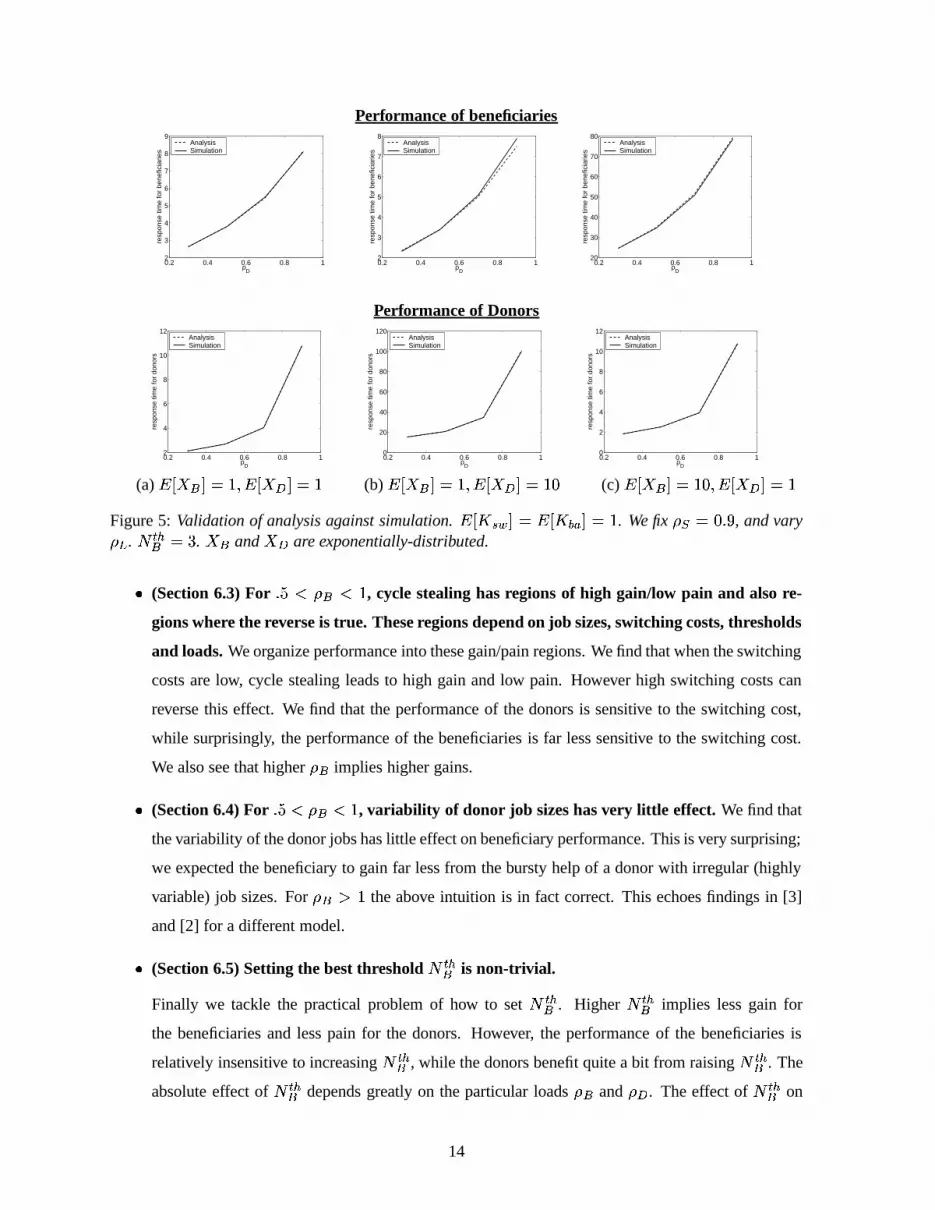
Figure 5: Validation of analysis against simulation.�� #" � � �

. We fix � � � � � � , and vary�� . � ��

. � � and � � are exponentially-distributed.

� (Section 6.3) For � � � � � � �, cycle stealing has regions of high gain/low pain and also re-

gions where the reverse is true. These regions depend on job sizes, switching costs, thresholds

and loads. We organize performance into these gain/pain regions. We find that when the switching

costs are low, cycle stealing leads to high gain and low pain. However high switching costs can

reverse this effect. We find that the performance of the donors is sensitive to the switching cost,

while surprisingly, the performance of the beneficiaries is far less sensitive to the switching cost.

We also see that higher � � implies higher gains.

� (Section 6.4) For � � � � � � � , variability of donor job sizes has very little effect. We find that

the variability of the donor jobs has little effect on beneficiary performance. This is very surprising;

we expected the beneficiary to gain far less from the bursty help of a donor with irregular (highly

variable) job sizes. For � � � �the above intuition is in fact correct. This echoes findings in [3]

and [2] for a different model.

� (Section 6.5) Setting the best threshold � �� is non-trivial.

Finally we tackle the practical problem of how to set �� . Higher � �� implies less gain for

the beneficiaries and less pain for the donors. However, the performance of the beneficiaries is

relatively insensitive to increasing � �� , while the donors benefit quite a bit from raising � �� . The

absolute effect of � �� depends greatly on the particular loads � � and � � . The effect of � �� on

14

Performance of beneficiary jobs

� ��

0 0.5 10

10

20

30

40

50

ρB

Res

pons

e tim

e fo

r be

nefic

iarie

s

0 0.5 10

10

20

30

40

50

ρB

Res

pons

e tim

e fo

r be

nefic

iarie

s

0 0.5 10

10

20

30

40

50

ρB

Res

pons

e tim

e fo

r be

nefic

iarie

s

0 0.5 10

10

20

30

40

50

ρB

Res

pons

e tim

e fo

r be

nefic

iarie

s

CS with NBth=1

CS with NBth=10

Dedicated

(a)�� (b) E[K]=1 (c) E[K]=0 (d) E[K]=1

Performance of donor jobs� ��

0 0.5 11.8

1.85

1.9

1.95

2

2.05

2.1

2.15

2.2

ρB

Res

pons

e tim

e fo

r do

nors

0 0.5 11.8

2

2.2

2.4

2.6

2.8

3

3.2

ρB

Res

pons

e tim

e fo

r do

nors

0 0.5 1

4.6

4.8

5

5.2

5.4

ρB

Res

pons

e tim

e fo

r do

nors

0 0.5 1

5

5.5

6

6.5

ρB

Res

pons

e tim

e fo

r do

nors

CS with NBth=1

CS with NBth=10

Dedicated

(a)�� (b) E[K]=1 (c) E[K]=0 (d) E[K]=1

Figure 6: The response time for beneficiaries and donors as a function of � � . Graphs show the case of (i)cycle stealing with � ��

, (ii) cycle stealing with � �� , and (iii) dedicated servers. In all figures� � and � � are exponential with mean 1. Switching cost is exponential with mean 0 or 1, as labeled.

mean performance (of beneficiaries and donors together) is irregular and delicate. In this section

we derive five rules of thumb for setting � �� as a function of the server loads, the switching costs,

and the donor job size.

Due to limited space we typically only show a couple options for each parameter. Many more graphs

are available in Appendix D.

6.2 Benefits of cycle stealing for wide range of ��

Figure 6 shows the response time for beneficiary jobs (top row) and donor jobs (bottom row) as a function

of � � , where � � is held fixed at � � � (columns 1 and 2) and at � � � (columns 3 and 4). Each graph shows

response time under (i) cycle stealing with � �� , (ii) cycle stealing with � �� , and (iii) dedicated

servers. The first and third columns have no switching cost, and the second and fourth columns have

exponential switching cost with mean 1.

When � � � � , cycle stealing can provide an infinite benefit to beneficiary jobs over dedicated servers.

We find that factors like increased switching costs, increased load at donor, and increased � �� all result

15

in lower gains for the beneficiary. However since the gain is infinite these factors are less important when

� � � � . We also see that the response time of donor jobs is bounded by the response time for an M/GI/1

queue with setup cost � , where � is the switch back cost. Increasing � �� results in less penalty to the

donor, converging to the same point for all � �� values when � � reaches its maximum.

When � � � � � � , the beneficiaries benefit so little that cycle stealing doesn’t pay, assuming non-zero

switching cost. We therefore focus the rest of the results section on the case: � � � � � � � � .6.3 Benefit of cycle stealing for

��

Gain of Beneficiaries and Loss of Donors — � ��

0.6 0.8 10

0.2

0.4

0.6

0.8

1

ρB

ρ D

low gainlow loss

mid gainlow loss

high gainlow loss

0.6 0.8 10

0.2

0.4

0.6

0.8

1

ρB

ρ D GOOD

0.6 0.8 10

0.2

0.4

0.6

0.8

1

ρB

ρ D

high gainhigh loss

mid gainmid loss

low gainlow loss

mid gainhigh loss

0.6 0.8 10

0.2

0.4

0.6

0.8

1

ρB

ρ D GOOD

BAD

(a)�� (b) E[K]=1


0.6 0.8 10

0.2

0.4

0.6

0.8

1

ρB

ρ D

low gainlow loss

mid gainlow loss

high gainlow loss

0.6 0.8 10

0.2

0.4

0.6

0.8

1

ρB

ρ D GOOD

0.6 0.8 10

0.2

0.4

0.6

0.8

1

ρB

ρ D

high gainhigh loss

high gainmid loss

mid gainmid loss

low gainlow loss

0.6 0.8 10

0.2

0.4

0.6

0.8

1

ρB

ρ D GOOD

BAD

(a)�� (b) E[K]=1

Figure 7: Columns 1 and 3 show the gain of beneficiary jobs and loss of donor jobs relative to dedicatedservers. High gain/loss refers to a

� � �� difference. Low gain/loss refers to a� � �� difference.

Columns 2 and 4 show the mean performance (over all jobs) relative to dedicated servers. In all figures:� � and � � are exponentially-distributed with mean 1.

Figures 7 and 8 evaluate cycle stealing in the region � � � � � � � � � � , as a function of � � . In Figure 7

� � and � � both have mean 1, while Figure 8 assumes � � has mean 1 and � � has mean 10. Both

figures assume switching cost is 0 or 1, and � �� is 1 or 3. In our discussion below, we first concentrate

on the effect of switching cost, and then look at the effect of �� .

A few definitions are necessary: The term “gain” refers to the improvement in mean response time

experienced by beneficiary jobs, as compared with dedicated servers. This gain is expressed as a per-

16


0.6 0.8 10

0.2

0.4

0.6

0.8

1

ρB

ρ D

low gainlow loss

mid gainlow loss

high gainlow loss

0.6 0.8 10

0.2

0.4

0.6

0.8

1

ρB

ρ D GOOD

0.6 0.8 10

0.2

0.4

0.6

0.8

1

ρB

ρ D

high gainlow loss

mid gainlow loss

low gainlow loss

0.6 0.8 10

0.2

0.4

0.6

0.8

1

ρB

ρ D GOOD

BAD

(a)�� (b) E[K]= 1


0.6 0.8 10

0.2

0.4

0.6

0.8

1

ρB

ρ D

low gainlow loss

mid gainlow loss

high gainlow loss

0.6 0.8 10

0.2

0.4

0.6

0.8

1

ρB

ρ D GOOD

0.6 0.8 10

0.2

0.4

0.6

0.8

1

ρB

ρ D

high gainlow loss

mid gainlow loss

low gainlow loss

0.6 0.8 10

0.2

0.4

0.6

0.8

1

ρB

ρ D GOOD

BAD

(a)�� (b) E[K]=1



Columns 2 and 4 show the mean performance (over all jobs) relative to dedicated servers. In all figures:� � and � � are exponentially-distributed, where � � has mean 1 and � � has mean 10.

centage of the mean response time under dedicated servers. The beneficiary jobs may experience low

gain (� � �� ), mid gain (between

� �� and� �� ), or high gain (

� � �� ). The term “loss” refers to the

relative pain (increase) in response time for donor jobs, as compared with dedicated servers. Loss is

also expressed as a percentage of the response time under dedicated servers. Odd-numbered columns

show various regions of gain and loss. Even-numbered columns use different terms: “good” and “bad.”

The “good” and “bad” terms refer to mean response time overall (over all jobs including beneficiaries

and donors). “Good” indicates that mean response time has dropped as a consequence of cycle stealing.

“Bad” indicates that mean response time has increased as a consequence of cycle stealing.

We start by looking at Figure 7. The first and second columns show the case of zero switching cost.

We see that all regions are low loss regions (in fact zero loss), and higher � � yields higher gain for

the beneficiaries. The third and fourth columns show switching cost of 1. The non-zero switching cost

creates slightly reduced gain for the beneficiaries (Recall from Section 6.2 that switching cost has a much

more pronounced effect on the beneficiaries when � � � � , as the beneficiary is dependent on the donor).

More importantly switching cost creates loss for the donor jobs. When � � is very low, the loss appears

17

high, but this is primarily due to the fact that “loss” is defined as a percentage relative to the response

time under dedicated servers, and the response time under dedicated servers is obviously low for small

� � . The mean gain over all jobs is no longer always positive as shown in the fourth column of Figure 7.

Although not shown, we have also investigated higher switching costs, and these lead to the same trend

of slightly less gain for beneficiaries and more loss for donors.

Figure 8 differs from Figure 7 only in � � which now has mean 10. The effect of this change is

dramatic: now a switching cost of 1 has almost no effect on either beneficiaries or donors. This makes

sense since the setup cost experienced by the donor job is now relatively small compared to its size. We

can conclude that cycle stealing is most effective when the switching cost is small relative to the size of

the donor jobs.

Consider now columns 2 and 4 of both figures, which depict the effect on overall mean response

time. When the switching cost is zero, cycle stealing always overwhelms the dedicated policy. When

switching cost is non-zero, cycle stealing is a good idea provided either � � is high, or the switching cost

is low compared to � � . These trends continue in our experiments with higher switching costs.

Finally, we discuss the effect of � �� in both figures. The performance of the beneficiaries is relatively

insensitive to increasing � �� from�

to�

in both figures; however the donors benefit quite a bit from

raising � �� . We further investigate selection of � �� in Section 6.5.

6.4 Effect of donor job size variability

In this section, we consider the effect of variability in the donor job sizes. It seems intuitive that when

donor job sizes are made more variable, two things should happen:

1. The donor pain percentage should go down. This is because the donor response times will be

higher overall and so the relative pain will appear to be less, and

2. The beneficiary gain should go down. This is because high variability in the donor job sizes,

implies high variability in the length of the donor busy periods, which implies that the donor’s

visits to the beneficiary queue will become more irregular. Sporadic help should be inferior to

regular help, for the beneficiary.

Figure 9 below shows that the first hypothesis above is in fact true, while the second hypothesis is

surprisingly false, at least for � � � � . Comparing row 1 ( � � has low variability: ��

) with row 2

( � � has high variability: ��

) we see that there is no discernible difference in donor performance.

To study this effect more closely, we next increase the variability in the donor job sizes to �� .

Figure 10 shows the performance of just the beneficiary jobs under the case of zero switching cost, when

the donor job size variability is 1, 8, or 50, and � � is fixed at 0.5. � � is allowed to vary from 0 to the

18

Gain of Beneficiaries and Loss of Donors — � � with ��

0.6 0.8 10

0.2

0.4

0.6

0.8

1

ρB

ρ D

low gainlow loss

mid gainlow loss

high gainlow loss

0.6 0.8 10

0.2

0.4

0.6

0.8

1

ρB

ρ D GOOD

0.6 0.8 10

0.2

0.4

0.6

0.8

1

ρB

ρ D

high gainhigh loss

high gainmid loss

mid gainmid loss

low gainlow loss

0.6 0.8 10

0.2

0.4

0.6

0.8

1

ρB

ρ D GOOD

BAD

(a)�� (b)

��

Gain of Beneficiaries and Loss of Donors — � � with ��

0.6 0.8 10

0.2

0.4

0.6

0.8

1

ρB

ρ D

mid gainlow loss

high gainlow loss

0.6 0.8 10

0.2

0.4

0.6

0.8

1

ρB

ρ D GOOD

0.6 0.8 10

0.2

0.4

0.6

0.8

1

ρB

ρ Dhigh gainhigh loss

high gainmid lossmid gain

mid loss

low gainlow loss

mid gainlow loss

0.6 0.8 10

0.2

0.4

0.6

0.8

1

ρB

ρ D GOOD

BAD

(a)�� (b)

��

Figure 9: Beneficiary gain and donor pain shown for donor job sizes with low variability (top) andhigh variability (bottom). Under higher donor variability, percentage of donor pain is lessened, butpercentage of beneficiary gain stays the same. All graphs assume: � � and � � have mean 1, � ��

.

stability condition. As is observed in Figure 9, the effect of variability of � � on the performance of � �

is very small when � � � � . When � � � � , the effect of variability in donor sizes is non-negligible, but

is still not as great as one might expect.

6.5 Optimal setting for beneficiary threshold, � ��

This section investigates the optimal setting for � �� . We start with some obvious rules: (i) increasing

� �� leads to lower gain for the beneficiaries and lower pain for the donors; (ii) if the switching cost is

zero, the optimal � �� is 1, since there is never any pain for the donors.

Figure 11 shows optimal values of � �� for minimizing mean response time over all jobs (donors

and beneficiaries) as a function of � � and � � under various switching costs and donor job sizes. The

numbers on the contour curves show the best � �� at each load. For clarity we only show lines up to

� �� . The following additional rules of thumb are implied by the figure: (iii) the optimal � �� is an

increasing function of � � and a decreasing function of � � ; (iv) increasing the switching cost increases

the optimal � �� ; (v) increasing the donor job size leads to lower optimal � �� .

19

Effect of variability of donor jobs on performance of beneficiary jobs

0 0.5 1 1.50

20

40

60

80

100

ρB

re

spon

se ti

me

for

bene

ficia

ries

ExpC2=8C2=50

Figure 10: The response time for beneficiary jobs under different donor job size variability. � � is fixedat 0.5. � � varies from 0 to the stability condition of 1.5. The mean donor job size and beneficiary jobsize is 1, and switching cost is zero.

Selecting the optimal � ��

�� ,��

,��

0.5 0.6 0.7 0.8 0.9

0.1

0.2

0.3

0.4

0.5

0.6

0.7

0.8

0.9

ρB

ρ D

22

4

46

68

8101214

0.5 0.6 0.7 0.8 0.9

0.1

0.2

0.3

0.4

0.5

0.6

0.7

0.8

0.9

ρB

ρ D

22

4

4

6

6

8

8

10

10

12

12

14

14

0.5 0.6 0.7 0.8 0.9

0.1

0.2

0.3

0.4

0.5

0.6

0.7

0.8

0.9

ρB

ρ D

2

23

34

4

56

0.5 0.6 0.7 0.8 0.9

0.1

0.2

0.3

0.4

0.5

0.6

0.7

0.8

0.9

ρB

ρ D 2

2

4

466

8

E[K]=1 E[K]=2 E[K]=1 E[K]=2

Figure 11: Graphs showing the optimal value of � �� with respect to mean response time over all jobs.

7 Extensions and Current Work

This paper solves the problem of cycle stealing with switching costs and thresholds, presenting many

insights into the characteristics and performance of cycle stealing. Our analytical approach easily gener-

alizes to more complex cycle stealing models. For example, in this paper we have assumed that the donor

immediately switches back when a donor job arrives. As we’ve stated earlier, we can also solve the more

general case where the donor only switches back when � �� donor jobs are waiting. Furthermore, we

don’t even need to require that the donor switches back immediately at this point; we can allow the donor

to first complete the beneficiary job in progress. Completing the beneficiary job obviates the need for

checkpointing the job, however it sometimes reduces system performance, particularly when beneficiary

jobs have higher variability than donor jobs. We can also handle the problem of one beneficiary and two

20

or more donors, where if � donors are helping, the beneficiary sees an �� . � � queue. This extension

also allows the different donors to have different switching thresholds and switching costs.

References[1] S. Asmussen. Phase-type distributions and related point processes: Fitting and recent advances. In S. R. Chakravarthy

and A. S. Alfa, editors, Matrix-Analytic Methods in Stochastic Models, pages 137–149. Marcel Dekker, 1997.

[2] S. Borst, O. Boxma, and P. Jelenkovic. Reduced-load equivalence and induced burstiness in gps queues with long-tailedtraffic flows. Under submission.

[3] S. Borst, O. Boxma, and M. van Uitert. The asymptotic workload behavior of two coupled queues. Under submission.

[4] J. Cohen and O. Boxma. Boundary Value Problems in Queueing System Analysis. North-Holland Publ. Cy., 1983.

[5] G. Fayolle and R. Iasnogorodski. Two couple processors: the reduction to a riemann-hilbert problem. Zeitschrift furWahrscheinlichkeitstheorie und vervandte Gebiete, 47:325–351, 1979.

[6] A. Konheim, I. Meilijson, and A. Melkman. Processor-sharing of two parallel lines. Journal of Applied Probability,18:952–956, 1981.

[7] G. Latouche and V. Ramaswami. Introduction to Matrix Analytic Methods in Stochastic Modeling. ASA-SIAM, Philadel-phia, 1999.

[8] M. F. Neuts. Matrix-Geometric Solutions in Stochastic Models. Johns Hopkins University Press, 1981.

[9] T. Osogami and M. Harchol-Balter. Matching three moments of distributions and busy periods by � -stage coxians.Technical Report CMU-CS-02-178, School of Computer Science, Carnegie Mellon University, September 2002.

[10] H. Takagi. Queueing Analysis – A Foundation of Performance Evaluation, volume 1: Vacation and Priority Systems, Part1. North Holland, 1991.

21

A Analysis of a variant: Donor switches back when unneeded

λB

λB

µB

µB

µB

λB

λB

λB

µB

λB

µB

λB

Dλ BDλD BD BD BD

BDλD

µB

λB

µB

λD

λB

µB

µB

2

λB

λB

λB

µB

µB

λD

µB

2

λB

λB

λB

µB

µB

λD

λD λDλD

Ksw Ksw Ksw

BD+baBD+ba

BD+ba BD+baBD+ba

Kba KbaKba

µB

2

µB

Bλ

λB

λB

µB

µB

DλDλDλ

0B,1D 1B,1D 2B,1D

0B,0D 1B,0D 2B,0D

4B,1D3B,1D

2B,1D,ba1B,1D,ba

2B,0D,C

4B,1D,ba

4B,0D,sw

4B,0D,C3B,0D,C

3B,0D,sw

3B,1D,ba

2B,0D,sw

0B,1D,ba

0B,0D,ba 1B,0D,ba 2B,0D,ba

Region 2

Region 1

Region 2

Figure 12: Markov chain of a variant. The donor server switches back when there is at most one benefi-ciary job regardless of the number of donor jobs.

In this section, we consider a variant of our algorithm: the donor server switches back when there is� �beneficiary job, even if there are no donor jobs at the time. One might imagine that the performance

of donor jobs would improve under this policy, especially when the arrival rate of donor jobs is high

compared to that of beneficiary jobs, and the cost of switching back is relatively high.

Figure 12 shows the Markov chain for the analysis of the variant in the case of � �� . It is assumed

that if the beneficiary server becomes idle while the donor server is still working on a beneficiary job,

then the job in progress at the donor server is passed over to the beneficiary server without any cost. It

is also assumed that �!� � , � #" , and � � are exponentially distributed, all of which can be generalized by

using Coxian distributions. The response time of the donor job is analyzed in the same way as before,

except that Region 2 in the chain has been expanded.

Having analyzed the above Markov chain, we find that counter to our intuition this variant does not

significantly affect the response time for the donor or the beneficiary, under all conditions studied.

22

B Incorporating a Donor threshold �� .

Throughout the paper we have assumed that the donor server switches back immediately when a new

donor job arrives at an empty donor queue. However, this is not necessarily the best policy with respect

to overall mean performance; given high switching costs, it might be better for the donor server to only

switch back if there are at least � �� donor jobs waiting. Furthermore, in Section 4 we found that the

stability region for the beneficiary is an increasing function of � �� , thereby giving further justification for

raising � �� . In this section, we show how to analyze a generalization of our algorithm, which assumes

general � �� .

Figure 13 shows a Markov chain that corresponds to cycle stealing where � �� " and � �� .

λB

λB

µB

µB

µB

λB

λB

λB

µB

λB

µB

λB

Dλ BDλD BD BD

λD

B2D+ba B2D+ba

λD

KswλD

λD

Ksw

λD

λD

KswλD

λD

Ksw

λB

λB

λB

λB

λB

µB

µB

µB

λD

λD

λD

λB

λB

λB

λB

λB

µB

µB

µB

µB

2

µB

2

Ksw

λD

Ksw

λD

λD

KswλD

λD

Ksw

B2D+ba

λB

λB

λB

λB

µB

µB

µB

2

µB

2

Ksw

λD

Ksw

λD

λD

KswλD

λD

Ksw

λB

λB

λB

λB

λB

µB

µB

µB

µB

2

µB

2

λB

µB

B2D+ba

BDBD

µB

µB

µB

λD

B2D+ba

0B,1D 1B,1D 2B,1D

0B,0D 1B,0D 2B,0D

4B,1D3B,1D

3B,1D,sw

3B,0D,sw

3B,0D,C

3B,1D,C

3B,2D,ba 4B,2D,ba

4B,1D,sw

4B,0D,sw

4B,0D,C

4B,1D,C

2B,2D,ba

2B,1D,sw

2B,0D,sw

2B,0D,C

2B,1D,C

1B,2D,ba

1B,1D,sw

1B,0D,sw

1B,0D,C

1B,1D,C

0B,2D,ba

0B,1D,sw

0B,0D,sw

0B,0D,C

0B,1D,C

Region B

Region A

Region D

Region C

Region C

Region C3

2

1

Figure 13: Markov chain for cycle stealing with � �� " and � �� and exponentially-distributed

� � and �� .

23

B.1 Response time for donor jobs

We first analyze the response time for donor jobs when � �� " . Then, the results are extended to

general � �� .

The states of the Markov chain are divided into four regions � , � , � , and � , where Region � is

further subdivided into three regions � � , � � , and � � , as shown in Figure 13. The time in queue for a

donor arrival is analyzed by conditioning on the region it arrives into. That is, the expected time in queue

is�� ! �#" $ ��%&"('*) �� ) ��

where�� +� � � � is the expected time in queue given that the arrival sees Region � .

When a donor job arrives in Region A, it sees a busy M/GI/1 queue, where the job sizes , � � and

the arrival rate is��

. Recall that the expected time in queue for an M/GI/1 is

��

�� " ��

which is also written as

�� -/. �10 ��243 � -5. �60 � � �� 87:9<; ��2=3 � �>7:9<; �where

�� -5. �60 �is the expected time in queue in an M/GI/1 given that the arrival finds the system

busy. Observing that�� 87:9<; � � � , and the probability that the system is busy is

243 � -5. �60 � �

� � � � � �� , we have

�� +� �@? � � �� -5. �10 ��

�� " ��

When a donor job arrives in Region B, the waiting time is zero, since the donor server is staying at

an empty donor queue. Thus,�� A�� CB � � �

To analyze the performance of a donor job, given that it arrives in Region C, first note that if we

aggregate Regions � � and � � into � �ED � , the duration of staying at Region � �ED � is exponentially distributed

with rate� �

, and the duration of staying at Region � � is the length of a busy period started by a job

of size � � and a setup time � � �� #" � � � . Furthermore, Region � � and Region � �ED � are visited

alternately; Regions A, B, and D are visited on the way from Region � � to Region � �ED � (see Figure 14).

Therefore, the fraction of time that the system spends in Region � � given that the system is either in

Region � � or in Region � �ED � is the same as the fraction of time that the M/GI/1 queue with setup time �

24

C2C3

C1

A

B

D

Figure 14: Transitions among regions of Markov chain in figure 13

is busy. The expected time in queue given that an arrival sees Region � � ( � �ED � , respectively) equals the

expected time in queue for an M/GI/1 queue with setup time, given that the arrival finds the system busy

(idle, respectively). Therefore, the expected time in queue given that an arrival sees Region C is just the

expected time in queue in a corresponding M/GI/1 queue with setup time � :

�� !��

� " �� " � � ��

� � � �� " � � � � �

When a donor job arrives in Region D, it waits for one more donor job to arrive, after which the

donor server switches back. Thus, the expected time in queue of an arrival into Region D is

�� A�� #" �

In summary, the time in queue for donor jobs is

�� -5. �60 ��! � �� +� � � � � �� E� �� ! �� ! � ��

� � � �� A��

The analysis is easily extended to general � �� . The Markov chain describing the states of such a

system can still be divided into four regions A, B, C, and D, but Region D is further divided into� �

regions � � , ..., � � � � (Region C is still subdivided into three regions, as before). In Region A, the donor

server is working on donor jobs. In Region B, the donor server is idle at the donor queue. In Region � � ,

the donor server is in the process of switching back to the donor queue. In Region � � , the donor server

is in the process of switching to the beneficiary queue and there are� �

donor jobs. In Region � � ,

the donor server is working on beneficiary jobs and there are� �

donor jobs. In Region � � , the donor

25

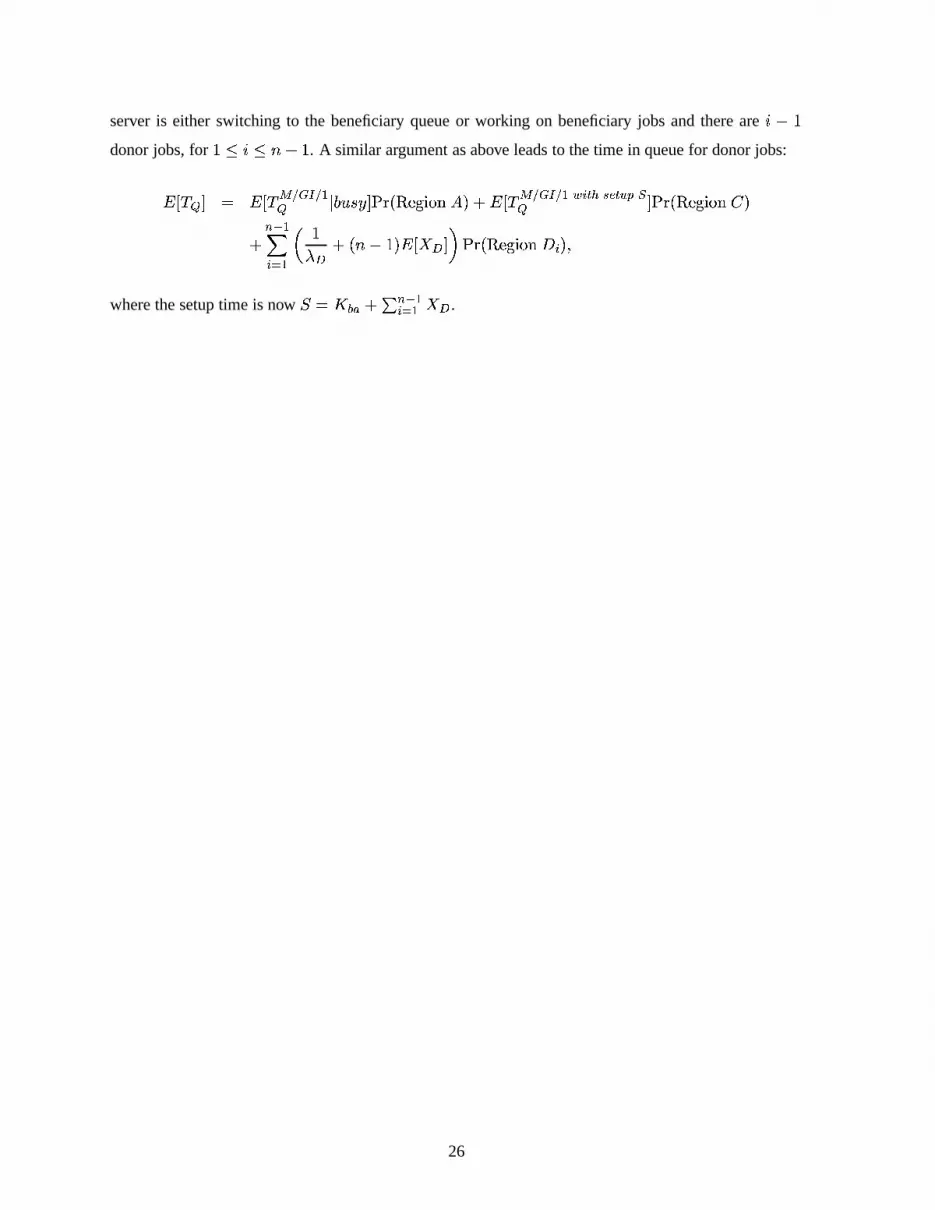
server is either switching to the beneficiary queue or working on beneficiary jobs and there are � �

donor jobs, for� �-�*� � �

. A similar argument as above leads to the time in queue for donor jobs:

�� -5. �60 ��! � �� +� � � � � �� E� �� ! �� ! � ��

� � ��

� �� A��

where the setup time is now � � �� #" �� ! � � � .

26

C Superposition of the chains

Figure 15 shows a superposition of the chains in Figure 1(b) and (c).

β2

b3 2b1

b2

b3b1

b2

β3β2β2β3

2b1b1

b3b1

β3

β1

b1

b3

b2

b1

b1

b2

b3

β3

β2β1

b3

b3

b3b3

b3

b3

b1b3

b1

b2

b1

b3

b3

b3

2b2

b3

b2

2b1

2b2

b2

2b2

b1

b1b3

b2

β2 β3

β1

λB

λDb2

b3b1XB

β1 β3

β2 ΒD

2b3

b2

2b3 2b3

b2

β1

b3

β2β3

β2 β3

β1

b3 b1

β2β3

β1

b2

b2

b1b3

b2

β1β2

β3β3

β1β1

β2

b1

b2b3β1

β2β3 β2

β3

β1


0B,1D 1B,1D 2B,1D

1B,0D0B,0D 2B,0D

4B,0D,C3B,0D,C

4B,1D3B,1D

β1

Figure 15: Markov chain for cycle stealing without switching cost, where � � and � � are both repre-sented by 2-stage Coxians.

27

D More graphs

In this section we include a few more result graphs omitted from the body of the paper for lack of space.

Figure 16 shows the gain/loss performance regions from Section 6.3 for the case where the beneficiaries

now have mean size 10 and the donors have mean size 1. The performance of the beneficiaries is virtually

identical to the case where � � and � � have mean 1. The donor performance is improved. The reason

for the improvement in donor performance is that the donor visits the beneficiary less frequently, since

the number of jobs queued at the beneficiary isn’t as high, for large jobs.

Figure 17 shows additional optimal � �� computations, for the case of large beneficiary jobs and the

case of highly variable donor jobs. The case of large beneficiary jobs, results in lower optimal � �� .

Increasing the variability of donor jobs doesn’t seem to have any effect.


0.6 0.8 10

0.2

0.4

0.6

0.8

1

ρB

ρ D

low gainlow loss

mid gainlow loss

high gainlow loss

0.6 0.8 10

0.2

0.4

0.6

0.8

1

ρB

ρ D GOOD

0.6 0.8 10

0.2

0.4

0.6

0.8

1

ρB

ρ Dlow gainlow loss

mid gainmid loss

high gainmid loss

high gainhigh loss

0.6 0.8 10

0.2

0.4

0.6

0.8

1

ρB

ρ D GOOD

BAD

(a)�� (b) E[K]= 1


0.6 0.8 10

0.2

0.4

0.6

0.8

1

ρB

ρ D

low gainlow loss

mid gainlow loss

high gainlow loss

0.6 0.8 10

0.2

0.4

0.6

0.8

1

ρB

ρ D GOOD

0.6 0.8 10

0.2

0.4

0.6

0.8

1

ρB

ρ D

low gainlow loss

mid gainlow loss

mid gainmid loss

high gainmid loss

0.6 0.8 10

0.2

0.4

0.6

0.8

1

ρB

ρ D GOOD

BAD

(a)�� (b) E[K]=1



Columns 2 and 4 show the mean performance (over all jobs) relative to dedicated servers. In all figures,� � and � � are exponentially-distributed, where � � has mean 10 and � � has mean 1.

28

Selecting the optimal � ��

�� , �� , � � : mean 1 and �

� � �

0.5 0.6 0.7 0.8 0.9

0.1

0.2

0.3

0.4

0.5

0.6

0.7

0.8

0.9

ρB

ρ D

2

4

46

68

8

10

10

1212

14

0.5 0.6 0.7 0.8 0.9

0.1

0.2

0.3

0.4

0.5

0.6

0.7

0.8

0.9

ρB

ρ D

2

4

46

6

8

8

10

10

12

12

14

14

0.5 0.6 0.7 0.8 0.9

0.1

0.2

0.3

0.4

0.5

0.6

0.7

0.8

0.9

ρB

ρ D

2

2

4

46

68

810

1214

0.5 0.6 0.7 0.8 0.9

0.1

0.2

0.3

0.4

0.5

0.6

0.7

0.8

0.9

ρB

ρ D

22

4

4

6

6

8

8

10

10

12

12

14

14

E[K]=1 E[K]=2 E[K]=1 E[K]=2

Figure 17: Graphs showing the optimal value of � �� with respect to mean response time over all jobs.

29

Documents

Analysis of cycle stealing with switching cost