Embed Size (px)
Citation preview
HAL Id: hal-03216762https://hal.inria.fr/hal-03216762
Submitted on 4 May 2021
HAL is a multi-disciplinary open accessarchive for the deposit and dissemination of sci-entific research documents, whether they are pub-lished or not. The documents may come fromteaching and research institutions in France orabroad, or from public or private research centers.
L’archive ouverte pluridisciplinaire HAL, estdestinée au dépôt et à la diffusion de documentsscientifiques de niveau recherche, publiés ou non,émanant des établissements d’enseignement et derecherche français ou étrangers, des laboratoirespublics ou privés.
Covert Cycle Stealing in a Single FIFO ServerBo Jiang, Philippe Nain, Don Towsley
To cite this version:Bo Jiang, Philippe Nain, Don Towsley. Covert Cycle Stealing in a Single FIFO Server. ACM Trans-actions on Modeling and Performance Evaluation of Computing Systems, ACM, In press, pp.1-35.hal-03216762
Covert Cycle Stealing in a Single FIFO Server
Bo Jiang ∗,1, Philippe Nain †,2, and Don Towsley ‡,3
1John Hopcroft Center for Computer Science, Shanghai Jiao Tong University, Shanghai, China2Inria, Ecole Normale Superieure de Lyon, LIP, 46 allee d’Italie, Lyon, 69364, France
3College of Information and Computer Sciences, University of Massachusetts, Amherst, MA,01003, USA.
May 4, 2021
Abstract
Consider a setting where Willie generates a Poisson stream of jobs and routes them to a single server thatfollows the first-in first-out discipline. Suppose there is an adversary Alice, who desires to receive servicewithout being detected. We ask the question: what is the number of jobs that she can receive covertly, i.e.without being detected by Willie? In the case where both Willie and Alice jobs have exponential servicetimes with respective rates µ1 and µ2, we demonstrate a phase-transition when Alice adopts the strategyof inserting a single job probabilistically when the server idles : over n busy periods, she can achieve acovert throughput, measured by the expected number of jobs covertly inserted, of O(
√n) when µ1 < 2µ2,
O(√n/ log n) when µ1 = 2µ2, and O(nµ2/µ1) when µ1 > 2µ2. When both Willie and Alice jobs have
general service times we establish an upper bound for the number of jobs Alice can execute covertly. Thisbound is related to the Fisher information. More general insertion policies are also discussed.
keywords: Cycle stealing; Covert communication; Queue.
1 Introduction
This paper considers the following problem. Willie has a sequence of jobs that arrive at a first-in first-out(FIFO) queue with a single server, whose processing rate is known to Willie. There exists another actor,Alice, who wants to sneak jobs into the queue for the purpose of stealing processing cycles from Willie.This paper asks the following question: can Alice process her jobs without Willie being able to determinethis occurrence beyond making a random guess and, if she can, what is her achievable job processing rate?Answers to this question may apply to several scenarios. Alice could administer a data center, contract toprovide Willie with a server with a guaranteed performance, and then resell some of the processing cycles[8]. Similar considerations apply to network contracts. Willie could own a home computer and Alice couldinstall malware for the purpose of stealing computational resources.
In order to address this question of covert cycle stealing, we adopt the following model. Willie’s jobs arriveaccording to a Poisson process to a FIFO queue served by a single server with a specified processing rate.
∗[email protected]†[email protected]‡[email protected]. The research of this author was supported by the US NSF grant CNS-1564067 and
the LABEX MILYON (ANR-10-LABX-0070) of Universit de Lyon, within the program "Investissements d’Avenir"
(ANR-11-IDEX- 0007) operated by the French National Research Agency (ANR).
1
Service times of Willie’s jobs are assumed to be independent and identically distributed (iid) according toa general distribution. Alice can insert jobs as she wishes. Her service times are also iid coming from ageneral distribution that may differ from that of Willie’s. Once an Alice job starts service, it must remainin service until completion; this can interfere with the processing of Willie’s jobs. Last, both Willie andAlice know their own and the other party’s service time distributions and can observe the arrival anddeparture times of Willie’s jobs.
We formulate the problem as a statistical hypothesis testing problem where Willie’s task is to determinewhether or not Alice is stealing cycles, based on observed arrivals and departures. We study the Insert-at-End-of-Busy-Period (IEBP) policy, where Alice (probabilistically) inserts a single job each time a Williebusy period (to be defined) ends. We obtain several results, of which the most interesting hold for expo-nential services for both Willie (rate µ1) and Alice (rate µ2) and establish that over n busy periods, Alicecan achieve a covert throughput – defined as the expected number of covertly inserted jobs – of O(
√n)
when µ1 < 2µ2, O(√n/ log n) when µ1 = 2µ2, and O(nµ2/µ1) when µ1 > 2µ2. This is interesting in part
because of the phase transition at µ1 = 2µ2; earlier studies of covert communications and in steganographyfocused on establishing O(
√n) behavior through the control of Alice’s parameters, avoiding regions in the
parameter space where this behavior might not hold.
In addition to the above results for the IEBP policy when service times are exponentially distributed, weshow that IEBP can also achieve a covert throughput of O(
√n) when Willie jobs have general service times
and Alice jobs have (hyper-)exponential service times, under some constraints on the service rates.
The rest of the paper is organized as follows. Section 2 discusses related work. Section 3 introduces themodel and needed background on hypothesis testing. Section 4 introduces the IEBP policy. Section 5 liststhe main results, and some preliminary results are established in Section 6. Sections 7-9 contain the proofsof the main results. Section 10 discusses alternative policies to the IEBP policy. Concluding remarks aregiven in Section 11.
A word on the notations. For any a ∈ [0, 1], let a := 1− a. We denote the convolution of f and g by f ∗ gand the n-fold tensor product of f with itself is denoted by f⊗n; recall that f⊗n(x1, . . . , xn) =
∏ni=1 f(xi)
with xi ∈ Rd (d ≥ 1). Throughout we use the shorthand notations ti:j for ti, . . . , tj for i < j, an ∼n bnfor limn→∞ an/bn = 1, and limn an (resp. lim infn an, lim supn an) for limn→∞ an (resp. lim infn→∞ an,lim supn→∞ an).
2 Related work
Cycle stealing has been analyzed in the queueing literature in the context of task assignment in multi-serversystems. The goal is to allow servers to borrow cycles from other servers while they are idle so as to reducebacklogs and latencies and prevent servers from being under-utilized [10, 17, 18]. These papers focus onthe performance analysis of such systems, in particular, mean response times with or without the presenceof switching costs. There is no attempt to hide or cover up the theft of cycles.
This paper focuses on the ability of an unknown user to steal cycles without the owner of the serverdetecting this. Thus it is an instance of a much broader set of techniques used in digital steganography andcovert communications. Steganography is the discipline of hiding data in objects such as digital images. Asteganographic system modifies fixed-size finite-alphabet covertext objects into stegotext containing hiddeninformation. A fundamental result of steganography is the square root law (SRL), O(
√n) symbols of an n
symbol covertext may safely be altered to hide an O(√n log n)-bit message [9]. Covert communications is
concerned with the transfer of information in a way that cannot be detected, even by an optimal detector.Here, there exists a similar SRL: suppose Alice may want to communicate to Bob in the face of a third party,Willie, without being detected by Willie. When communication takes place over a channel characterized by
2
additive white Gaussian noise, it has been established that Alice can transmit O(√n) bits of information
in n channel uses [3]. This result has been extended to optical (Poisson noise) channels [2], binary channels[6], and many others [5, 21]. It has also been extended to include the presence of jammers [20], and tonetwork settings [19]. Like our work, both steganography and covert communications rely on the use ofstatistical hypothesis testing. One difference from covert communications is that in our setting Alice hidesher jobs in exponentially distributed noise (Willie’s service times) and sometimes generally distributednoise, whereas Alice hides in zero mean Gaussian noise in covert communications. In addition, in thecommunications context, Alice has control over the power that she transmits at whereas in our context,Alice does not control the size of her jobs, only the rate at which they are introduced.
This work also has ties to the detection of service level agreement (SLA) violation problem. Detecting SLAviolation in today’s complex computing infrastructures, such as clouds infrastructures, presents challengingresearch issues [8]. However no careful analysis of this problem has been conducted. Our work may providean avenue to doing such.
During the review process a paper related to ours appeared [22]. In [22] Alice’s jobs arrive continuouslyaccording to a Poisson process with rate λb. It is shown that if Willie knows the number of his jobssuccessively served in a busy period and λb lies below a certain threshold, then the expected number ofjobs that Alice can covertly insert over n busy periods is O(
√n). If instead Willie knows the length of
each busy period instead, the expected number of jobs that Alice can covertly insert is only O(1).
3 Model and Background
This section gives details about the model we use in the present work and the needed background onhypothesis testing. As mentioned in the introduction, there is a legitimate user, Willie, who sends asequence of jobs to a single server with known service rate. There is also an illegitimate user, Alice, whowants to introduce a sequence of jobs to be serviced. The questions that we address are the following: canAlice covertly introduce her stream of jobs, i.e. without Willie being able to tell with confidence whethershe has introduced the stream or not, and if so, at what rate can she introduce her jobs? We answer thesequestions under the following assumptions:
1. Willie jobs arrive at the server according to a Poisson process with rate λ ∈ (0,∞);
2. the service times of all jobs are independent;
3. the service time distributions are known to both parties;
4. the server serves all jobs in a FIFO manner;
5. once in service, Alice jobs cannot be preempted;
6. Willie observes only his arrivals and departures;
7. Alice observes Willie’s and her own arrivals and departures.
The first four assumptions are made mainly for tractability. If Alice jobs can be preempted whenevera Willie job arrives, then Alice can hide her jobs during Willie’s idle periods without affecting his jobs.Consequently, we make the fifth assumption to make the problem interesting. Note that allowing Alice toalso observe Willie arrivals and departures gives her the capability to identify idle periods within which tohide her jobs.
Assumption 6 implies that Willie does not know the state of the server. If he does then Alice can onlytransmit during busy periods. However, if the scheduling policy is FIFO (Assumption 4) Alice cannot
3
know if an inserted job of hers will not be the last one of the busy period, in which case it will be detectedby Willie; relaxing the FIFO assumption appears to be very challenging.
Assume that the system is empty at time 0. Denote by Ai and Di the arrival and departure times of Willie’si-th job, respectively, for i ≥ 1. We assume that D0 = 0. Note that 0 < Ai < Ai+1 and 0 < Di < Di+1. LetA1:m = A1, . . . , Am, D1:m = D1, . . . , Dm. Let S1:m = (S1, . . . , Sm) denote the reconstructed servicetimes of the first m jobs, which satisfy the following recurrence relation,
Si =
D1 −A1, i = 1,
Di −maxAi, Di−1, i ≥ 2.(1)
These are the service times perceived by Willie. Note that (A1:m, S1:m) and (A1:m, D1:m) contain the sameinformation, as they uniquely determine each other. It is also all the information available to Willie in ourmodel.
We define a Willie Busy Period (W-BP) to be the time interval between the arrival of a Willie job thatfinds no other Willie job in the system and the first subsequent departure of a Willie job that leaves noother Willie jobs in the system. Let Mj denote the number of Willie’s jobs served in the first j W-BPs,which can be defined recursively by M0 = 0 and
Mj = min i > Mj−1 : Ai+1 > Di , j ≥ 1. (2)
Let Nj = Mj −Mj−1 denote the number of Willie jobs served in the j-th W-BP.
Willie’s observation is W1:n, where
Wj :=(Mj = mj , A(mj−1+1):mj = a(mj−1+1):mj , S(mj−1+1):mj = s(mj−1+1):mj
), j = 1, . . . , n. (3)
In words, Willie observes n W-BPs and for each W-BP records the number of his jobs that have beenserved, their arrival times and reconstructed service times.
The null hypothesis H0 is that Alice does not insert jobs and the alternative hypothesis H1is that Aliceinserts jobs. Willie’s test may incorrectly accuse Alice when she does not insert jobs, i.e. he rejects H0
when it is true. This is known as type I error or false alarm, and, its probability is denoted by PFA [15]. Onthe other hand, Willie’s test may fail to detect insertions of Alice’s jobs, i.e. he accepts H0 when it is false.This is known as type II error or missed detection, and its probability is denoted by PMD. Assume thatWillie uses classical hypothesis testing with equal prior probabilities of each hypothesis being true. Then,the lower bound on the sum PE = PFA + PMD characterizes the necessary trade-off between false alarmsand missed detections in the design of a hypothesis test. If prior probabilities are not equal, P(H0) = π0
and P(H1) = π1, then, PE ≥ min(π0, π1)(PFA + PMD) [3, Sec. V.B]. Hence scaling results obtained forequal priors apply to the case of non-equal priors and we focus on the former in the remainder of the paper.
4 Insert-at-End-of-Busy-Period Policy
In this section, we consider the strategy that Alice inserts a job probabilistically at the end of each W-BP,which we call the Insert-at-End-of-Busy-Period (IEBP) Policy. Note that there may be an Alice job inthe system at the start of a W-BP. This occurs when Alice has inserted a job at the end of a W-BP andthat her job has not completed service by the time the next Willie job arrives.
Throughout the section, we assume that Willie jobs have service time distribution G1 with continuous pdfg1 and finite mean 1/µ1 > 0, and that Alice jobs have service time distribution G2 with continuous pdf g2
4
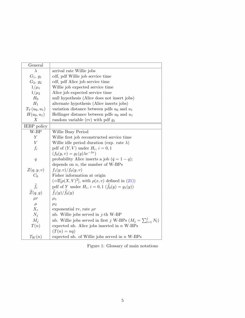
General
λ arrival rate Willie jobsG1, g1 cdf, pdf Willie job service timeG2, g2 cdf, pdf Alice job service time1/µ1 Willie job expected service time1/µ2 Alice job expected service timeH0 null hypothesis (Alice does not insert jobs)H1 alternate hypothesis (Alice inserts jobs)
TV (u0, u1) variation distance between pdfs u0 and u1
H(u0, u1) Hellinger distance between pdfs u0 and u1
X random variable (rv) with pdf g1
IEBP policy
W-BP Willie Busy PeriodY Willie first job reconstructed service timeV Willie idle period duration (exp. rate λ)fi pdf of (Y, V ) under Hi, i = 0, 1
(f0(y, v) = g1(y)λe−λv)q probability Alice inserts a job (q = 1− q);
depends on n, the number of W-BPsZ(q, y, v) f1(y, v)/f0(y, v)
C0 Fisher information at origin(=E[ρ(X,V )2], with ρ(x, v) defined in (21))
fi pdf of Y under Hi, i = 0, 1 (f0(y) = g1(y))
Z(q, y) f1(y)/f0(y)µr µ1
µ µ2
Xr exponential rv, rate µrNj nb. Willie jobs served in j-th W-BP
Mj nb. Willie jobs served in first j W-BPs (Mj =∑j
l=1Nl)T (n) expected nb. Alice jobs inserted in n W-BPs
(T (n) = nq)TW (n) expected nb. of Willie jobs served in n W-BPs
Figure 1: Glossary of main notations
5
and finite mean 1/µ2 > 0. Denote by G∗i (s) =∫∞
0 e−sxgi(x)dx the Laplace Stieltjes transform (LST) of gifor i = 1, 2. We also assume λ/µ1 < 1 so that the system is stable under H0.
4.1 Introducing the IEBP Policy
To motivate the IEBP policy, we first find the minimum probability that an Alice job interferes withWillie’s jobs. Suppose an Alice job is inserted at time t, with service time σ2 ∼ G2. Let Ut ≥ 0 be theunfinished work (of both Alice and Willie jobs) in the system just before time t. The newly inserted Alicejob will affect Willie if he sends a job in the interval (t, t+ Ut + σ2), the probability of which is
P(at least one Willie job arrives in (t, t+ Ut + σ2))
≥ P(at least one Willie job arrives in (t, t+ σ2))
=
∫ ∞0
P(at least one Willie job arrives in (t, t+ x))g2(x)dx
=
∫ ∞0
(1− e−λx)g2(x)dx = 1−G∗2(λ) := p. (4)
Thus if Alice is to insert a single job then she should insert it when the system is idle so as to minimize theprobability of interfering with a Willie job. Motivated by this observation, we introduce the IEBP policybelow.
Alice’s strategy. Alice inserts a job with probability q at the end of each W-BP. We refer to this as theInsert-at-End-of-Busy-Period (IEBP) policy. Given that Alice does insert a job, the probability that itinterferes with a Willie job is given by p in (4). Thus pq is the probability that an interference occurs in agiven W-BP.
4.2 Willie’s Detector
It is not easy to work directly with the observation process W1:n defined in (3) (Section 3). Instead, wewill work with the statistic (Y1:n, V1:n), with Yj denoting the reconstructed service time of the first Williejob in the j-th W-BP and Vj the length of the idle period preceding it. These quantities are given by
Yj = SMj−1+1, (5)
Vj = AMj−1+1 −DMj−1 . (6)
Denote by fi(y, v) the joint pdf of (Y, V ) at (Y = y, V = v) under Hi for i = 0, 1. Also, let fi(y) :=∫∞0 fi(y, v)dv denote the pdf of Y at Y = y under Hi for i = 0, 1. Under H0 the system is a standardM/G/1 queue; in particular, the random variables (rvs) Y and V are independent with pdf g1(y) andλe−λv, respectively, yielding
f0(y, v) = g1(y)λe−λv, (7)
f0(y) = g1(y). (8)
Under H1, Yj is the sum of the remaining service time of Alice’s job, if any, when a Willie job initiatesthe j-th W-BP, and of the service time of this Willie’s job. Therefore, under H1 the system is an M/G/1queue with arrival rate λ, exceptional first service time in a busy period with pdf f1, and all other servicetimes (the ordinary customers) in a busy period with pdf g1. In Proposition 5.5 (Section 5) we derive someperformance metrics of interest for this queueing system.
6
An important feature of the process (Y1:n, V1:n) is that (Y1, V1), . . . , (Yn, Vn) form iid rvs due to the Poissonnature of Willie job arrivals and the assumptions that Willie’s and Alice’s service times are mutuallyindependent processes, further independent of the arrival process. This is the main benefit from using thestatistic (Y1:n, V1:n) instead of the statistic Wn. From now on (Y, V ) denotes a generic (Yj , Vj).
The independence of the rvs (Y1, V1), . . . , (Yn, Vn) under Hi (i = 0, 1) implies that their joint pdf is givenby f⊗ni , the n-th fold tensor product of fi with itself.
The following lemma shows that (Y1:n, V1:n) is a sufficient statistic (e.g. see [15, Chapter 1.9]), that is,Willie does not lose any information by considering the statistic (Y1:n, V1:n) instead of the statistic W1:n inorder to detect the presence of Alice. The proof is given in Appendix A.
Lemma 4.1. For every n ≥ 1, (Y1:n, V1:n) is a sufficient statistic.
Theorem 13.1.1 in [15] is established in the case where a simple hypothesis P0 is tested against a simplealternative P1. In our setting, q = 0 is the simple hypothesis against the simple alternative q = q(n), andwe are asking how we can scale q(n) down to 0 so that we can not differentiate q = 0 and q = q(n), withn the number of observed W-BPs.
Theorem 1. ([15, Theorem 13.1.1])
Using the observed values (y1:n, v1:n) of (Y1:n, V1:n), any test accepting H0 if∏ni=1 f0(yj , vj) >
∏ni=1 f1(yj , vj)
and rejecting H0 if∏ni=1 f0(yj , vj) <
∏ni=1 f1(yj , vj) minimizes PE. Furthermore, the minimum PE is given
byP ?E = 1− TV
(f⊗n0 , f⊗n1
),
where
TV (u0, u1) =1
2
∫|u0(x)− u1(x)|dx (9)
is the total variation distance between two distributions with densities u0 and u1, respectively.
We will henceforth assume that for a given (Y1:n, V1:n) Willie uses the above optimal test.
We say that Alice’s insertions are covert provided that, for any ε > 0, she has an insertion strategy foreach n such that
lim infn
P ?E ≥ 1− ε, (10)
or equivalently from Theorem 1, if for any ε > 0,
lim supn
TV(f⊗n0 , f⊗n1
)≤ ε. (11)
Note that a sufficient condition for Alice’s insertions not being covert is that for some δ ∈ (0, 1) there existsa detector such that
lim supn
PE < δ. (12)
Here the limit is taken over the number of busy periods that Willie observes. This covertness criterion wasproposed in the context of low probability of detection (LPD) communications in [3].
Theorem 1 suggests using the total variation distance to analyze Willie’s detectors. However, the totalvariation distance is often unwieldy even for products of pdfs, like f⊗n0 and f⊗n1 . To overcome this drawback,it is common (e.g. see [3]) to use the following Pinsker’s inequality (Lemma 11.6.1 in [7])
TV (u0, u1) ≤ KL(u0‖u1), (13)
7
where KL(u0‖u1) :=∫Rd u0(x) ln u0(x)
u1(x)dx is the Kullback-Leibler (KL) divergence between the probabilitydistributions with pdf u0 and u1, respectively.
However, we will work with the Hellinger distance, which has the advantage of offering both lower andupper bounds on the total variation distance. The Hellinger distance between two probability distributionswith pdf u0 and u1 respectively, denoted H(u0, u1), is defined by
H(u0, u1) =1
2
∫Rd
(√u0(x)−
√u1(x)
)2dx. (14)
Note that
H(u0, u1) = 1−∫Rd
√u0(x)u1(x)dx, (15)
and 0 ≤ H(u0, u1) ≤ 1. It is known [13, Lemma 4.1] that
H(u0, u1) ≤ TV (u0, u1) ≤√
2H(u0, u1). (16)
The upper bound (resp. lower bound) in (16) will be used to establish covert (resp. non-covert) results.
We will also use the following well-known property of the Hellinger distance between pdfs u⊗n0 and u⊗n1
[16, Eq. (1.4)]:
H(u⊗n0 , u⊗n1
)= 1−
∫Rd
n∏j=1
√u0(xj)u1(xj)
n∏j=1
dxj by (15)
= 1−(∫
Rd
√u0(x)u1(x)dx
)n. (17)
5 Main Results
Let T (n) denote the expected number of jobs that Alice inserts in n W-BPs. Under the IEBP policy,
T (n) = nq. (18)
This section presents the main results that characterize T (n) under various conditions as n becomes large.Implicit in all asymptotic results as n→∞ is that q is a function of n.
Recall that fi(y, v) is the joint pdf of (Y, V ) at (Y = y, V = v) under Hi for i = 0, 1, with f0 given in (7).The likelihood ratio
Z(q, y, v) :=f1(y, v)
f0(y, v), (19)
plays an important role in determining how many jobs Alice can insert covertly. It is shown in Lemma B.1in Appendix B that Z has the following form,
Z(q, y, v) = 1 + qρ(y, v), (20)
where
ρ(y, v) :=1
g1(y)
∫ y
0g1(u)g2(v + y − u)du−G2(v). (21)
Since ρ(y, v) does not depend on the insertion probability q, this shows that the likelihood ratio Z(q, y, v)depends linearly on q. Define
C0 := E[ρ(X,V )2], (22)
8
where (X,V ) has pdf f0(x, v) at (x, v).
It is worth noting that C0 = J(0), with J(q) := E[(
ddq log f1(X,V )
)2]
the Fisher information of (Y, V )
about the parameter q. Indeed, since f1(x, v) = f0(x, v)(1 + qρ(x, v)) by (19)-(20), we have
J(q) =
∫1
f1(x, v)2
(d
dqf1(x, v)
)2
f0(x, v)dxdv =
∫ρ(x, v)2
(1 + qρ(x, v))2f0(x, v)dxdv,
and therefore J(0) = E[ρ(X,V )2]. The Fisher information evaluates the amount of information that arandom variable carries about an unknown parameter [14].
Proposition 5.1 gives the covert throughput for general service time distributions. Its proof is given inSection 7.
Proposition 5.1 (Covert throughput for general service time distr. and finite C0). Assume C0 <∞.Under the IEBP policy, the number of jobs Alice can insert covertly is T (n) = O(
√n) if E[ρ(X,V )] = 0,
and T (n) = O(1) if E[ρ(X,V )] 6= 0.
Remark 1. E[ρ(X,V )] = 0 for any pdf g1 if g2 is the pdf of an exponential or an hyper-exponential rv.Indeed, when g2(x) = µ2e
−µ2x, ρ(x, v) in (21) writes
ρ(x, v) = e−µ2v
((g1 ∗ g2)(x)
g1(x)− 1
). (23)
By the independence of X and V and the fact that g1 ∗ g2 is a pdf,
E[ρ(X,V )] = E[e−µ2V ] · E[(
(g1 ∗ g2)(X)
g1(X)− 1
)]= 0. (24)
The proof when g2 is the pdf of an hyper-exponential rv is a simple generalization. Note that E[ρ(X,V )]does not always vanish. In particular, E[ρ(X,V )] 6= 0 when G2 is an Erlang distribution. Indeed, when
g2(x) = (kµ2)k
(k−1)!xk−1e−kµ2x, k ≥ 1 (Alice service times follow a k-Erlang distribution with mean 1/µ2), it is
easy to show that for any pdf g1, E[ρ(X,V )] = (1−G∗2(λ))(
(kµ2)k
µ2− 1)6= 0 for all k > 1.
The next lemma gives conditions for C0 <∞ under various distributional assumptions. Its proof is foundin Appendix C.
Lemma 5.2 (Finiteness of C0).
1. Suppose both Alice and Willie have exponential service times, i.e. gi(x) = µie−µix for i = 1, 2. Then
C0 <∞ if and only if µ1 < 2µ2.
2. Suppose both Alice and Willie have hyper-exponential service times, i.e.
gi(x) =
Ki∑l=1
pi,lµi,le−µi,lx,
where∑Ki
l=1 pi,l = 1, for i = 1, 2. Then C0 <∞ if and only if
max1≤l≤Ki
µ1,l ≤ 2 min1≤m≤K2
µ2,m.
9
3. Suppose Willie has Erlang service times and Alice has hyper-exponential service times, i.e.
g1(x) =νK1
1
(K1 − 1)!xK1−1e−ν1x
and
g2(x) =
K2∑l=1
p2,lµ2,le−µ2,lx,
where∑K2
l=1 p2,l = 1. Then C0 <∞ if and only if
ν1 < 2 min1≤l≤K2
µ2,l.
Proposition 5.1 gives sufficient conditions for Alice to be covert. This raises the following questions:
Q1: When C0 <∞, can Alice insert covertly more than O(√n) jobs on average during n W-BPs?
Q2: When C0 =∞, what is the maximum number of jobs that Alice can insert covertly on average duringn W-BPs?
We do not have full answers to the above questions. Proposition 5.3 first gives a necessary condition forAlice to be covert under IEBP. Proposition 5.4 then provides a partial answer for the IEBP policy whenboth Alice and Willie have exponential service times. Proofs are found in Sections 8 and 9.
Proposition 5.3 (Necessary condition for covertness).
Under IEBP Alice cannot be covert if lim supn→∞ q > 0.
Consider now the situation when limn→∞ q = 0. The result below is the main result of the paper.
Proposition 5.4 (Covert throughput and converse for exponential service time distr.). Assume thatgi(x) = µie
−µix for i = 1, 2, and Alice uses the IEBP policy with limn→∞ q = 0. She can be covert if
T (n) =
O(√n), if µ1 < 2µ2,
O(√n/ log n), if µ1 = 2µ2,
O(nµ2/µ1), if µ1 > 2µ2.
(25)
She cannot be covert if
T (n) =
ω(√n), if µ1 < 2µ2,
ω(√n/ log n), if µ1 = 2µ2,
ω(nµ2/µ1), if µ1 > 2µ2.
(26)
The above results are in terms of T (n), the expected number of jobs inserted by Alice over n successiveW-BPs. It is interesting to determine also the expected number of Willie jobs served during these n W-BPs under the IEBP policy. Let TW (n) be this number. When q = 0, the system behaves like a standardM/G/1 queue with traffic intensity λ/µ1 < 1 and it is known that the expected number of jobs served ina busy period is (1− λ/µ1)−1 [12], yielding TW (n) = n(1− λ/µ1)−1. Proposition 5.5 below shows that theIEBP policy increases each W-BP by a constant factor. The proof is in Appendix H.
10
Proposition 5.5. Under IEBP, TW (n) = Θ(n). More precisely
TW (n) =n
1− λ/µ1+
λqn
1− λ/µ1
∫ ∞0
tg2(t)dt, (27)
which gives the two-sided inequality
n ≤ TW (n) ≤ n(
1 + qλ/µ2
1− λ/µ1
). (28)
If g2(x) = µ2e−µ2x, i.e. Alice job service times are exponentially distributed, then
TW (n) = n
(1 + pqλ/µ1
1− λ/µ2
). (29)
Remark 2. Recall that the Fisher information regarding q is infinity at q = 0 when µ1 ≥ µ2. It is interestingto speculate that this translates into facilitating Willie’s detection task, which appears in the form of thephase transition in equations (25) and (26). Note that one implication of this transition is that Alice shouldselect job sizes with mean size 1/µ2 < 2/µ1 to increase throughput without being detected.
6 Preliminary results
We first specialize the two-sided inequality in (16) to the case where u0 = f⊗n0 and u1 = f⊗n1 and thendevelop a covert (resp. non-covert) criterion for Alice.
Lemma 6.1. The Hellinger distance between f⊗n0 and f⊗n1 is given by
H(f⊗n0 , f⊗n1
)= 1−
(E[√
Z(q,X, V )])n
. (30)
Proof. By (17) and (19),
H(f⊗n0 , f⊗n1
)= 1−
(∫[0,∞)2
√f0(y, v)f1(y, v) dydv
)n= 1−
(∫f0(y, v)
√Z(q, y, v) dydv
)n= 1−
(E[√
Z(q,X, V )])n
.
Specializing (16) to the value of H(f⊗n0 , f⊗n1
)found in Lemma 6.1 gives,
Lemma 6.2 (Lower & upper bounds on total variation distance for statistic Yj , Vjj). For every n ≥ 1
1−(E[√
Z(q,X, V )])n≤ TV
(f⊗n0 , f⊗n1
)≤√
2(
1−(E[√
Z(q,X, V )])n)
. (31)
Combining Lemma 6.2, the covert criterion (11), and the non-covert criterion (12) yields the followingcovert/non-covert criterion for Alice:
11
Corollary 6.1 (Covert/non-covert criteria for the IEPB policy).Assume that Willie uses an optimal detector for the sufficient statistic (Y1:n, V1:n). Alice’s insertions are
covert if for any ε > 0,
lim infn
(E[√
Z(q,X, V )])n≥ 1− ε, (32)
and Alice’s insertions are not covert if for any δ > 0
lim supn
(E[√
Z(q,X, V )])n
< δ. (33)
The lower bound (32) is used to derive the covert throughput (25) in Proposition 5.4.
We now state and prove a non-covert criterion for the IEPB policy. We do so by proposing and analyzinga detector that relies on the (non-sufficient) statistic Yjj . Recall that rvs Y1, . . . , Yn are iid with common
pdf fi(y) under Hi, for i = 0, 1. The non-covert criterion is obtained by applying Theorem 13.1.1 in [15]
to the statistic Y1:n, which yields the minimum PE to be 1− TV(f⊗n0 , f⊗n1
).
The following lemmas are the analog of Lemmas 6.1 and 6.1 for the statistic Yj.
Lemma 6.3. The Hellinger distance between f⊗n0 and f⊗n1 is given by
H(f⊗n0 , f⊗n1
)= 1−
(E[√
Z(q,X)
])n, (34)
with
Z(q, x) :=f1(x)
g1(x). (35)
Lemma 6.4 (Lower bound on total variation distance for statistic Y1:n). For every n ≥ 1
1−(E[√
Z(q,X)
])n≤ TV
(f⊗n0 , f⊗n1
). (36)
The proof of Lemma 6.3 mimics that of Lemma 6.1 and is omitted. Lemma 6.4 follows from Lemma 6.3and the lower bound in (16).
The non-covert criterion for the statistic Yjj announced earlier is given below. Its proof follows from(12) and (36).
Corollary 6.2 (Non-covert criterion for the IEPB policy).Assume that Willie uses an optimal detector for the statistic Yjj. Alice’s insertions are not covert if for
any δ > 0
lim supn
(E[√
Z(q,X)
])n< δ. (37)
Corollary 6.2 is used in the proofs of Proposition 5.3 and of the converse (26) in Proposition 5.4.
Remark 3. In direct analogy with the upper bound in Lemma 6.2 it is worth noting that TV
(f⊗n0 , f⊗n1
)in Lemma 6.4 is upper bounded by
√2
(1−
(E[√
Z(q,X)
])n). However, this bound is not useful for
establishing a covert result since it does not use the sufficient statistic (Y1:n, V1:n).
12
7 Proof of Proposition 5.1
The proof of Proposition 5.1 relies on an upper bound on the total variation distance between f⊗n0 andf⊗n1 , given in Lemma 7.1 below. Recall the definition of ρ(X,V ) given in (21).
Lemma 7.1. Let (X,V ) be rvs with density f0. Assume that E[ρ(X,V )] = 0. Then, for every n ≥ 1,
TV(f⊗n0 , f⊗n1
)≤ 1
2
√(1 + q2C0)n − 1, (38)
where C0 is defined in (22).
Proof. Let (Xj , Vj)j be iid rvs with pdf f0. By (9),
2TV(f⊗n0 , f⊗n1
)=
∫[0,∞)2n
∣∣∣∣∣∣n∏j=1
f0(yj , vj)−n∏j=1
f1(yj , vj)
∣∣∣∣∣∣n∏j=1
dyjdvj
=
∫[0,∞)2n
n∏j=1
f0(yj , vj)
∣∣∣∣∣∣1−n∏j=1
Z(q, yj , vj)
∣∣∣∣∣∣n∏j=1
dyjdvj
= E
∣∣∣∣∣∣1−n∏j=1
Z(q,Xj , Vj)
∣∣∣∣∣∣ , (39)
where the second equality follows from (19).
Using the inequality E|U | ≤√E[U2] in (39) yields
(2TV
(f⊗n0 , f⊗n1
))2 ≤ 1− 2E
n∏j=1
Z(q,Xj , Vj)
+ E
n∏j=1
Z(q,Xj , Vj)
2= 1− 2 [EZ(q,X, V )]n +
[E[Z(q,X, V )2]
]n(40)
= −1 +(1 + 2qE[ρ(X,V )] + q2E[ρ(X,V )2]
)n= −1 +
(1 + q2E[ρ(X,V )2]
)n,
where we have used the value of Z(q, x, v) obtained in (80) in Appendix B and the assumption thatE[ρ(X,V )] = 0 to establish the last two identities.
We are now in position to prove Proposition 5.1.
Proof of Proposition 5.1. In order to compute the covert throughput, assume that Willie uses an optimaldetector for the sufficient statistic (Yj , Vj), j = 1, . . . , n. Let
q =δ
φ(n),
with δ ∈ (0, 1] and φ : 1, 2, . . . → [1,∞), so that by (18)
T (n) =δn
φ(n). (41)
13
First consider the case E[ρ(X,V )] = 0. Note that T (n) = O(√n) implies
lim supn
√n
φ(n)<∞. (42)
By Lemma 7.1
supk≥n
TV
(f⊗k0 , f⊗k1
)≤ sup
k≥n
1
2
√(1 +
δ2C0
φ(k)2
)k− 1 ∼ δ
√C0
2supk≥n
k
φ(k)2, as n→∞
as limn φ(n) =∞ by Lemma D.1 in Appendix D. Therefore,
lim supn
TV(f⊗n0 , f⊗n1
)≤ δ√C0
2
(lim sup
n
√n
φ(n)
)2
. (43)
By making δ small enough, lim supn TV (f⊗n0 , f⊗n1 ) can be made arbitrarily small. We then conclude from(10) that Alice is covert when T (n) = O(
√n), which completes the proof for the case E[ρ(X,V )] = 0.
Now consider the case E[ρ(X,V )] 6= 0. Note that T (n) = δnφ(n) = O(1) implies there exist k > 0 and n0
such that for all n ≥ n0, 0 ≤ nφ(n) ≤ k. Using inequality (40) and the definition of Z(q, y, v) in (20) gives
(2TV
(f⊗n0 , f⊗n1
))2≤ 1− 2e
n log(
1+ δφ(n)
E[ρ(X,V )])
+ en log
(1+ 2δ
φ(n)E[ρ(X,V )]+ δ2
φ(n)2C2
0
)
∼ 1− 2eE[ρ(X,V )] δn
φ(n) + e2E[ρ(X,V )] δn
φ(n)+δ2C2
0n
φ(n)2 , (44)
as n → ∞. Since nφ(n) and n
φ(n)2 are bounded away from infinity as n → ∞, we see that the r.h.s. of (44)
can be made arbitrarily close to 0 by letting δ → 0. We then conclude from (10) that Alice is covert whenT (n) = O(1), which completes the proof.
8 Proof of Proposition 5.3
The proof uses Corollary 6.2. Take q = 1φ(n) with lim supn q > 0 or, equivalently, lim infn φ(n) <∞.
Assume that Willie uses an optimal detector for the statistic Yjj so that Corollary 6.2 applies. Recall
(cf. Section 6) that f1(y) (resp. g1(y)) is the pdf of Y under H1 (resp. H0), with Z(q, y) = f1(y)g1(y) being the
associated likelihood ratio.
We first derive properties of Z(q, y), to be used in this proof and in the proof of Proposition 5.4.
We claim that
Z(q, y) =
∫ ∞0
λe−λvZ(q, y, v)dv. (45)
Indeed by (19) and (7)∫ ∞0
λe−λvZ(q, y, v)dv =1
g1(y)
∫ ∞0
f1(y, v)dv =f1(y)
g1(y)= Z(q, y),
from the definition of Z(q, y) in (35). Hence by (20)
Z(q, y) = 1 + qρ(y), (46)
14
with
ρ(y) :=
∫ ∞0
λe−λvρ(y, v)dv
=1
g1(y)
∫ ∞0
λe−λv∫ y
0g1(u)g2(v + y − u)dudv −
∫ ∞0
λe−λvG2(v)dv by (21)
=(g1 ∗ g2)(y)
g1(y)− p, (47)
by using the definition of p in (4), and where
g2(t) :=
∫ ∞0
λe−λvg2(v + t)dv. (48)
We are now ready to prove Proposition 5.3. Recall that X is a rv with pdf g1. We have
E[√
Z(q,X)
]=
∫ √√√√ 1∏i=0
fi(x)dx ≤
√√√√ 1∏i=0
∫fi(x)dx = 1, (49)
by Cauchy-Schwarz inequality. Equality holds in (49) if and only if (see e.g. [1, p. 14]) f1(x) = cf0(x)for some constant c > 0. Since both f0 and f1 are densities, integrating over [0,∞) yields c = 1, which is
equivalent to q = 0 from (35) and (46). This shows that E[√
Z(q,X)
]< 1 if and only if 0 < q ≤ 1.
Since lim infn φ(n) := d < ∞ by assumption, there exists a subsequence of φ(n)n, say φ(kn)n, suchthat φ(kn) ≥ d with limn φ(kn) = d.
Let M := sup1/d≤q≤1 E[√
Z(q,X)
]. Note
√Z(q,X) =
√1 + qρ(X) ≤
√1 + |ρ(X)| ≤ 1 + |ρ(X)|. By
(47), E[|ρ(X)|] ≤∫
(g1 ∗ g2)(t)dt + p and g1 ∗ g2 is integrable as both g1 and g2 are integrable. The
Dominated Convergence Theorem then guarantees that the function q 7→ E[√
Z(q,X)
]is continuous.
Since E[√
Z(q,X)
]< 1 for all q ∈ [1/d, 1] as shown above, we have M < 1. Therefore,
E[√
Z(1/φ(kn), X)
]≤M < 1
for all n. As a result
limn
(E[√
Z(1/φ(kn), X)
])n= 0,
which implies from Corollary 6.2 that Alice’s insertions are not covert when lim infn φ(n) < 0, or equiva-lently when lim supn q =∞.
9 Proof of Proposition 5.4
Throughout this section, we assume that Alice and Willie job service times are exponentially distributedwith rate µ2 and µ1, respectively, namely, gi(x) = µie
−µix for i = 1, 2.
The proof of Proposition 5.4 relies on Corollaries 6.1 and 6.2, and Lemma 9.1 below. Before stating thelatter, let us introduce some notation.
15
Let µ1 = rµ and µ2 = µ. For r 6= 1, define β = rr−1 and note that r = β
β−1 and 1 − β = 1r−1 . Let Xr
denote an exponential rv with rate µr.
For θ ∈ [0, 1], x ≥ 0, define
Ξ(θ, x) =
1 + θ(µx− 1) if r = 1
1 + θ(e(r−1)µx
r−1 − β)
if r 6= 1.(50)
By specializing Z(q, x, v) in (20) to the case where gi(x) = µie−µix for i = 1, 2, we obtain from (23) that
Z(q, x, v) = Ξ(qe−µv, x), ∀q ∈ [0, 1], x ≥ 0, v ≥ 0. (51)
One the other hand, by (45) and the fact that Ξ(θ, x) is linear in θ,
Z(q, x) =
∫ ∞0
λe−λvΞ(qe−µv, x)dv = Ξ(
∫ ∞0
qλe−(λ+µ)vdv, x) = Ξ(pq, x), ∀q ∈ [0, 1], x ≥ 0, (52)
where we have used that p = λ/(µ2+λ) (see (4)) when Alice job service times are exponentially distributed.
For θ ∈ [0, 1], define
ξr(θ) :=(β − 1)θ
1− βθ, (53)
for r ≥ 2 (i.e. 1 < β ≤ 2), and
Iβ := β
∫ ∞0
1 + 12 t−
√t+ 1
tβ+1dt, (54)
for r > 2. Since β ∈ (1, 2) when r > 2, the generalized integral Iβ is finite and positive.
Lemma 9.1. For θ ∈ [0, 1], define
Fr(θ) :=
1−r
4(r−2)θ + o(θ)2) if 0 < r < 114ξ
22(θ) log ξ2(θ) + ∆2(ξ2(θ)) if r = 2
−Iβξβr (θ) + ∆r(ξr(θ)) if r > 2,
(55)
where, for t > 0,
∆r(t) :=
o(t2 log t) if r = 2o(tβ) if r > 2.
(56)
Then, for r ∈ (0, 1) ∪ [2,∞),
E[√
Ξ(θ,Xr)]
= 1 + Fr(θ), 0 ≤ θ ≤ 1. (57)
The proof of Lemma 9.1 is given in Appendix E.
Since ξr(θ) defined in (53) will only be evaluated at θ = qe−µv with q = δ/φ(n) and δ ∈ [0, 1], thereby
yielding ξr(θ) = (β−1)δeµvφ(n)−βδ , we omit the argument θ in ξr(θ) to simplify notation.
We are now ready to prove Proposition 5.4. Recall that at the beginning of an idle period, Alice inserts ajob with probability q(n) = δ
φ(n) , δ ∈ (0, 1], with
limnφ(n) =∞.
16
Henceforth we drop the argument n in q(n). Furthermore
T (n) = nq =δn
φ(n)(58)
is the expected number of Alice’s insertions in n W-BPs.
9.1 Proof of (25)
We assume that Willie uses an optimal detector for the sufficient statistic (Yj , Vj)j , which allows us toapply Corollary 6.1.
9.1.1 Case µ1 < 2µ2
The proof follows from Proposition 5.1 since E[ρ(X,V )] = 0 when Alice and Willie job service times areexponentially distributed (cf. Remark 1) and since C0 <∞ when µ1 < 2µ2, as shown in Lemma 5.2-(1).
9.1.2 Case µ1 = 2µ2
Without loss of generality we assume in this section that
φ(n) ≥ 8, ∀n ≥ 1. (59)
This assumption is motivated by the need to have log φ(n) > 2 (for the proof of Lemma F.2 in AppendixF).
Recall that X2 denotes an exponential rv with rate 2µ. By Lemma 9.1,(E[√
Z(δ/φ(n), X2, V )])n
=
(1 +
∫ ∞0
λe−λv(
1
4ξ2
2 log ξ2 + ∆2(ξ2)
)dv
)n= e
n log
(1+∫∞0 λe−λv ξ2
2 log ξ2×(
14
+∆2(ξ2)
ξ22 log ξ2
)dv
), (60)
with ∆2(z) = o(z2 log z) and ξ2 = δe−µv
φ(n)−2δe−µv > 0 for all n ≥ 1 and for all v ≥ 0 thanks to (59). For v ≥ 0
notice that ξ2 > 0 for all n and ξ2 → 0 as n→∞. Define
Dn :=
∫ ∞0
λe−(λ+2µ)v log ξ2
(φ(n)− 2δe−µv)2
(1
4+
∆2(ξ2)
ξ22 log ξ2
)dv, (61)
so that (60) rewrites (E[√
Z(δ/φ(n), X2, V )])n
= en log(1+δ2Dn). (62)
The proof of (25) for µ1 = 2µ2 consists in showing that, as n→∞, the r.h.s. of (62) can be made arbitraryclose to one by selecting δ small enough, and to apply (32) in Corollary 6.1.
The first step is to show that Dn → 0 as n → ∞. This result is shown in Lemma F.1 in Appendix F.Hence, (
E[√
Z(δ/φ(n), X2, V )])n
∼n eδ2nDn (63)
17
from (62). The second step is to show that nDn is bounded as n → ∞. This result is shown in LemmaF.2 in Appendix F under the condition that T (n) = O(
√n/ log n).
The proof is concluded as follows: when T (n) = O(√n/ log n), by (63) and Lemma F.2, as n →
∞,(E[√
Z(δ/φ(n), X2, V )])n
can be made arbitrarily close to one by taking δ small enough. The proof
of (25) for µ1 = 2µ2 then follows from (32) in Corollary 6.1.
9.1.3 Case µ1 > 2µ2
Fix r > 2 so that 1 < β < 2. By Lemma 9.1(E[√
Z(δ/φ(n), Xr, V )])n
= en log
(1+∫∞0 λe−λv
(−Iβξβr +∆r(ξr)
)dv)
= en log(1+δβ(β−1)βEn), (64)
with ∆r(z) = o(zβ), ξr = δ(β−1)eµvφ(n)−βδ , and
En := −∫ ∞
0λe−λv
Iβ −∆r(ξr)/ξβr
(eµβφ(n)− δβ)βdv. (65)
Lemma F.3 in Appendix F states that En → 0 as n→∞ and Lemma F.4 in Appendix F states that nEnis bounded as n→∞ when T (n) = O(nµ2/µ1). Therefore, cf (64),(
E[√
Z(δ/φ(n), Xr, V )])n∼n eδ
β(β−1)βnEn , (66)
and when T (n) = O(nµ2/µ1) as n→∞ the r.h.s. of (66) can be made arbitrarily close to one by selectingδ small enough. The proof of (25) for µ1 > 2µ2 then follows from (32) in Corollary 6.1.
9.2 Proof of (26)
We assume that Willie uses an optimal detector for the statistic Yjj , which will allows us to use thenon-covert criterion in Corollary 6.2. Since the proofs in Sections 9.2.1-9.2.3 will not depend on δ ∈ (0, 1],we assume without loss of generality that δ = 1, yielding q = 1
φ(n) and T (n) = nφ(n) .
9.2.1 Case µ1 < µ2
Assume that T (n) = ω(√n), or equivalently
limn→∞
n
φ(n)2=∞. (67)
Assume first that 0 < r < 1. From (52) and Lemma 9.1 we obtain(E[√
Z(p/φ(n), Xr)
])n= e
n log
(1+ p2
4 ( 1−rr−2)/φ(n)2+o(1/φ(n)2)
)
∼n en
φ(n)2p2
4 ( 1−rr−2)
as φ(n)→∞ as n→∞∼n 0, (68)
18
where the latter follows from (67) together with 1−rr−2 < 0 when 0 < r < 1. We invoke Corollary 6.2 to
conclude that Alice is not covert when T (n) = ω(√n) and 0 < r < 1.
It remains to show that Alice is not covert for 1 ≤ r < 2 when T (n) = ω(√n) with limn n/φ(n)2 = ∞.
Without any additional effort, we will prove a stronger result (to be used in the proof of the case µ1 = 2µ2
of (26)) that Alice is not covert when T (n) = ω(√n) and r ≥ 1. By applying Lemma G.1 in Appendix G
to (52), we obtain
E[√
Z(p/φ(n), Xr′)
]≤ E
[√Z(p/φ(n), Xr)
](69)
for any r′ ≥ r. Combining now (69) and (68) readily yields
limn→∞
(E[
√Z(p/φ(n), Xr′)
)n= 0
for any r′ ≥ 1. Similarly to the case 0 < r < 1 we then conclude from Corollary 6.2 that Alice is notcovert T (n) = ω(
√n) and r ≥ 1. In summary, we have shown that Alice is not covert for all r > 0 when
T (n) = ω(√n).
9.2.2 Case µ1 = 2µ2
Assume that T (n) = ω(√n/ log n) or, equivalently,
limn
φ(n)√n log n
= 0. (70)
From (52) and Lemma 9.1(E[√
Z(p/φ(n), X2)
])n= en log(1+ 1
4ξ22 log ξ2+o(ξ2
2 log ξ2)), (71)
with ξ2 = pφ(n)−2p . Since ξ2 ∼n 0 when limn φ(n) =∞, we have
ξ2 log ξ2 → 0 as n→∞.
Therefore, from (71), (E[√
Z(p/φ(n), X2)
])n∼n e
n4ξ22 log ξ2 . (72)
We have proved in the case µ1 < 2µ2 of (26) that Alice is not covert for all r > 0 when T (n) = ω(√n).
As a result, it suffices to focus on T (n) satisfying (70) when T (n) 6= ω(√n). The latter is equivalent to
φ(n) = Ω(√n), that is,
lim infn
φ(n)√n> 0. (73)
We have
nξ22 log ξ2 =
p2(φ(n)√n logn
− 2p√n logn
)2
(log p
log n− log(φ(n)− 2p)
log n
)
∼n−p2(
φ(n)√n logn
− 2p√n logn
)2 ×log(φ(n)− 2p)
log n. (74)
19
By (70) the first factor in the r.h.s. of (74) converges to −∞ as n→∞. Let us focus on the second factor.We have
log(φ(n)− 2p)
log n=
1
2+
log(φ(n)−2p√
n
)log n
∼n1
2+
log(φ(n)√n
)log n
.
Assumption (73) ensures thatlog(φ(n)√n
)logn → 0 as n→∞ and
log(φ(n)− 2p)
log n→ 1
2as n→∞.
In summary, we have shown that nξ22 log ξ2 → −∞ as n → ∞ which, in turn, implies from (72) that
limn
(E[√
Z(p/φ(n), X2)
])n= 0. We conclude from Corollary 6.2 that Alice is not covert if r = 2 and
T (n) = ω(√n/ log n).
9.2.3 Case µ1 > 2µ2
Assume that T (n) = n/φ(n) = ω(nµ2/µ1) or, equivalently,
limn
φ(n)
nβ= 0. (75)
Let r > 2 so that β ∈ (1, 2). From (57),(E[√
Z(p/φ(n), Xr)
])n= e
n log(
1−Iβξβr +o(ξβr ))
∼n e−Iβnξβr , (76)
since ξr = (β−1)pφ(n)−βp → 0 when limn φ(n) =∞. We have
nξβr =(β − 1)p)β(φ(n)nβ− βp
nβ
)β → +∞ as n→∞.
Introducing the above limit in (76) and using the finiteness and positiveness of Iβ for β ∈ (1, 2), gives
limn
(E[√
Z(p/φ(n), Xr)
])n= 0, which shows by using again Corollary 6.2 that Alice is not covert if
r > 2 and T (n) = ω(nµ2/µ1).
This concludes the proof of Proposition 5.4.
10 Other policies
The first policy – called the Insert-at-Idle (II) policy – is a variant of the IEBP policy and works as follows:Alice inserts a job with probability q each time the server idles, and stop inserting with probability q(before she tries again at the end of the next W-BP). The difference between the IEBP and II policies is
20
that under the former Alice inserts at most one job between the end of a W-BP and the start of the nextW-BP, whereas under the II policy she may insert more than one job during this time period.
It is shown in [11, Section 5] that when Alice job service times are exponentially distributed all covert/non-covert results obtained under the IEBP policy hold under the II policy. The intuition behind this is thatwhen Alice job service times are exponentially distributed, Willie sees ”the same system behavior” undereither policy; indeed, under either policy a job of his can interfere with at most one Alice job in a W-BP,whose remaining service time is exponentially distributed.
We have observed at the beginning of Section 4.1 that Alice should preferably inserts jobs at idle times;this was the motivation for introducing and investigating the IEBP policy in Section 4 and its variant, theII policy. But can Alice submit more jobs covertly if she also inserts jobs at other times than at idle times,typically, just after an arrival /departure of a Willie job? Note that, because of the FIFO assumption,Alice cannot benefit from inserting a job at a time t+ if time t is neither an arrival time nor a departuretime of a Willie job.
This is the motivation for introducing the class of the so-called Insert-at-Idle-and-at-Arrivals (II-A) policies,in which
• each time the server idles Alice inserts one job with probability q and does not insert a job withprobability q;
• after the arrival of each Willie job, Alice inserts a batch of s ≥ 0 jobs with probability qQ(s) and withprobability 1− q she does not insert any job.
Notice that the II-A policy reduces to the II policy when QB(0) = 1 (no job inserted at arrival times).Only non-covert results are obtained in [11, Section 6]. More specifically, for exponential service times forboth Alice and Willies, Alice is non-covert if T (n) = ω(
√n) when the support of Q is finite. A variant of
the II-A policy is when Alice inserts a batch of jobs that is geometrically distributed at times the serverbecomes idle and immediately after the arrival of a Willie job, both with probability q. Non-covert resultsare also obtained for this policy. The obtained results indicate that batching may be harmful and thatAlice should insert only one job at a time.
11 Concluding remarks
In this paper we have studied covert cycle stealing in an M/G/1 queue. We have obtained a phase transitionresult on the expected number of jobs that Alice can covertly insert in n busy periods when both Aliceand Willie’s jobs have exponential service times and established partial covert results for arbitrary servicetimes. Several research directions present themselves. We conjecture that Proposition 5.4 holds for amore general class of distributions; it would be interesting to verify this. It would be useful to weakenthe assumption that Willie’s detectors rely on observations being independent and identically distributedrandom variables; this would lead to consideration of a larger class of policies on Alice’s behalf. Anotherdirection would be to allow Alice to control her job sizes and study what benefit this would provideher. Yet another is to consider other hypothesis testing techniques including generalized likelihood ratiotest (GLRT), sequential detection, etc. GLRT could lead to relaxing the need for Willie to know Alice’sparameters whereas sequential detection could lead to more timely detection of Alice.
21
References
[1] G. Bachmann and L. Narici. Fourier and Wavelet Analysis. Springer Science & Business Media, 2012.
[2] B.A. Bash, A.H. Gheorghe, M. Patel, J.L. Habif, D. Goeckel, D. Towsley, and S. Guha. Quantum-secure covert communication on bosonic channels. In Nature Communications, volume 6, 2015.
[3] B.A. Bash, D. Goeckel, and D. Towsley. Square root law for communication with low probabilityof detection on awgn channels. In Proc. IEEE Int. Symp. Inform. Theory (ISIT), pages 448–452,Cambridge, MA, USA, July 2012.
[4] U.N. Bhat. On the busy period of a single server bulk queue with modified service mechanism. CalcuttaStatist. Assoc. Bull., 13:163–171, 1964.
[5] M.R. Bloch. Covert communication over noisy channels: A resolvability perspective. IEEE Trans.Inf. Theory, 62(5):2334–2354, 2016.
[6] P.H. Che, M. Bakshi, C. Chan, and S. Jaggi. Reliable deniable communication with channel uncer-tainty. In Proc. IEEE Int. Symp. Inform. Theory Workshop, pages 448–452, July 2013.
[7] T.M. Cover and J.A. Thomas. Elements of Information Theory. John Wiley & Sons, 2nd edition,2002.
[8] V. Emeakaroha, M. Netto T. Ferreto, I. Brandic, and C. De Rose. Casvid: Application level moni-toring for SLA violation detection in clouds. In IEEE Annual Computer Software and ApplicationsConference (COMPSAC), pages 499–508, Cambridge, MA, USA, July 2012.
[9] J. Fridrich. Steganography in Digital Media: Principles, Algorithms, and Applications. CambridgeUniversity Press, 2009.
[10] M. Harchol-Balter, C. Li, T. Osogami, A. Scheller-Wolf, and M. Squillante. Analysis of task assignmentwith cycle stealing under central queue. In Proc. Fifteenth ACM Annual Symposium on ParallelAlgorithms and Architectures, pages 274–285, San Diego, June 2003.
[11] B. Jiang, P. Nain, and D. Towsley. Covert cycle stealing in a single fifo server (extended version).https://arxiv.org/abs/2003.05135, 2021.
[12] L. Kleinrock. Queueing Systems, Vol. 1: Theory. Wiley-Interscience, 1975.
[13] C.H. Kraft. Some Conditions for Consistency and Uniform Consistency of Statistical Procedures,volume 2, pages 125–142. Univ. California Publications in Statist., 1955.
[14] S. Kullback. Information Theory and Statistics. Dover, 1968.
[15] E. Lehmann and J. Romano. Testing Statistical Hypotheses. New York: Springer, 3rd edition, 2005.
[16] J. Oosterhoff and W. R. Van Zwet. A note on contiguity and hellinger distance. In MathematischeStatistiek, volume 36. Stichting Mathematisch Centrum, 1975.
[17] T. Osogami, M. Harchol-Balter, and A. Scheller-Wolf. Analysis of cycle stealing with switching timesand thresholds. In ACM Sigmetrics, pages 184–195, San Diego, CA, Junw 2003.
[18] T. Osogami, M. Harchol-Balter, and A. Scheller-Wolf. Analysis of cycle stealing with switching timesand thresholds. Performance Evaluation, 61(4):347–369, 2005.
22
[19] A. Sheikholeslami, M. Ghaderi, D. Towsley, B. Bash, S. Guha, and D. Goeckel. Multi-hop routing incovert wireless networks. IEEE Trans. Wireless Communications, 17(6):3656–3669, 2018.
[20] T.V. Sobers, B.A. Bash, S.K. Guha, D. Towsley, and D. Goeckel. Covert communication in thepresence of an uninformed jammer. IEEE Trans. Wireless Communications, 16(9):6193–6206, 2017.
[21] L. Wang, G.W. Wornell, and L. Zheng. Fundamental limits of communication with low probability ofdetection. IEEE Trans. on Information Theory, 62(6):3493–3503, 2016.
[22] A. Yardi and T. Bodas. A Covert Queueing Problem with Busy Period Statistic. IEEE CommunicationLetters, 2020.
A Appendix: Proof of Lemma 4.1
Let pi,n(w1:n) be the pdf of W1:n = (W1, . . . ,Wn) at w1:n = (w1, . . . , wn) under Hi for i = 0, 1. Also letpi,j(wj) be the pdf 1 of Wj at wj under Hi for i = 0, 1. Note that pi,n (resp. pi,j) is a generalized pdf sinceW1:n (resp. Wj) contains integer and continuous components.
By the general multiplicative formula,
pi,n(w1:n) = pi,1(w1)×n∏j=2
pi,j(wj |W1:j−1 = w1:j−1). (77)
Let wj = (mj , a(mj−1+1):mj , s(mj−1+1):mj ), yj = smj−1+1, and vj = amj−1+1 − dmj−1 . We have
pi,j(wj |W1:j−1 = w1:j−1) = pi,j(wj |Amj−1 = amj−1 , Dmj−1 = dmj−1 , Amj−1+1 > dmj−1),
since the probability distribution of the number of customers served in a busy period in an M/G/1 queueis entirely determined once we know the duration of the first service time in this busy period [12, Chapter5.9]. Hence,
pi,j(wj |W1:j−1 = w1:j−1) = 1(amj−1+1 > dmj−1
)fi(yj , vj)
×p(Mj = mj , A(mj−1+2):mj = a(mj−1+2):mj , S(mj−1+2):mj = s(mj−1+2):mj |Yj = yj , Vj = vj
), (78)
where the latter density is independent of H0 and H1. The pdf pi,1(w1) is given by the r.h.s. of (78) byletting j = 1. Putting (77) and (78) together yields the factorization result
pi,n(w1:n) =
n∏j=1
fj(yj , vj)× other factors independent of H0 and H1, (79)
which proves that (Y1:n, V1:n) is a sufficient statistic [15, Chapter 1.9].
B Appendix
Recall that Z(q, y, v) = f1(y,v)f0(y,v) , with fi(y, v) the pdf of (Y, V ) at (y, v) under Hi for i = 0, 1.
1Clearly pi,j(wj) =∫Rn−1 pi,n(w1:n)dw1 · · · dwj−1dwj+1 · · · dwn.
23
Lemma B.1.Z(q, y, v) = 1 + qρ(y, v), (80)
where
ρ(y, v) :=1
g1(y)
∫ x
0g1(u)g2(v + y − u)du−G2(v). (81)
Proof. Consider a generic W-BP. Let σ1 (resp. σ2) denote a generic service time of a Willie (resp. Alice)job. Let A be the event that Alice inserts a job at the end of the W-BP. Then
Y = σ1 + 1A · (σ2 − V )+,
where (z)+ = maxz, 0. We first compute the conditional density f1(y | v) of Y given V . Given AC ,Y = σ1, so
f1(y | v,Ac) = g1(y).
Given A and V = v, we have Y = σ1 + (σ2 − v)+, so that
f1(y | v,A) = g1(y)G2(v) +
∫ y
0g1(u)g2(y + v − u)du.
Recall the probability of A under H1 is q, so
f1(y | v) = qf1(y | v,A) + qf1(y | v,Ac)
= g1(y) + q
[∫ y
0g1(u)g2(y + v − u)du− g1(y)G2(v)
]= g1(y)[1 + qρ(y, v)], (82)
by using the definition of ρ(y, v) in (81). Therefore,
Z(q, y, v) =f1(y | v)λe−λv
f0(y, v)= 1 + qρ(y, v),
by using (7), which concludes the proof.
C Appendix: Proof of Lemma 5.2
Let g2(x) =∑K2
l=1 p2,lg2,l(x) with g2,l(x) := µ2,le−µ2,lx, p2,l ≥ 0 for all l and
∑K2l=1 p2,l = 1, namely, Al-
ice job service times follow an hyper-exponential distribution with mean 1/µ2 =∑K2
l=1 1/µ2,l. Denote byG∗1(s) =
∫∞0 e−sxg1(x)dx the Laplace transform of Willie job service times.
By using (21), we find
ρ(x, v) =1
g1(x)
K2∑l=1
p2,le−µ2,lv(g1 ∗ g2,l)(x)−
K2∑l=1
p2,le−µ2,lv,
so thatE[ρ(X,V )2
]= α1 − 2α2 + α3
with
α1 :=
∫[0,∞)2
λe−λv
g1(x)
[K2∑l=1
p2,le−µ2,lv(g1 ∗ g2,l)(x)
]2
dvdx
24
=
K2∑l=1m=1
λp2,lp2,m
µ2,l + µ2,m
∫ ∞0
(g1 ∗ g2,l)(x)× (g1 ∗ g2,m)(x)
g1(x)dx;
α2 :=
K2∑l=1m=1
p2,lp2,m
∫[0,∞)2
λe−(λ+µ2,l)v(g1 ∗ g2,l)(x)eµ2,mxdvdx
=
K2∑l=1m=1
p2,lp2,mλµ2,lG
∗1(µ2,m)
(λ+ µ2,l)(µ2,l + µ2,m)≤ 1;
α3 :=
K2∑l=1m=1
p2,lp2,m
∫[0,∞)2
λe−λvg1(x)e−(µ2,l+µ2,m)xdvdx
=
K2∑l=1m=1
p2,lp2,mG∗1(µ2,l + µ2,m) ≤ 1.
We conclude from the above that E[ρ(X,V )2] <∞ if and only if
βl,m :=
∫ ∞0
(g1 ∗ g2,l)(x)× (g1 ∗ g2,m)(x)
g1(x)dx <∞ (83)
for all l,m = 1, . . . ,K2.
Case 1: g1(x) =∑K1
i=1 p1,iµ1,ie−µ1,ix, p1,i ≥ 0 for all i and
∑K1i=1 p1,i = 1, namely, Willie job service times
follow an hyper-exponential distribution with mean 1/µ1 =∑K1
i=1 1/µ1,i.
We have
(g1 ∗ g2,l)(x) =
K1∑i=1
p1,iµ1,iµ2,l
[xe−µ2,lx 1(µ1,i = µ2,l) +
e−µ2,lx − e−µ1,ix
µ1,i − µ2,l1(µ1,i 6= µ2,l)
]
for l = 1, . . . ,K2, so that
(g1 ∗ g2,l)(x)× (g1 ∗ g2,m)(x) =
K1∑i=1j=1
p1,ip1,jµ1,iµ1,j
[Pi,l(x)Pj,m(x)e−(µ2,l+µ2,m)x
−ai,lbj,mxe−(µ1,i+µ2,m)x − aj,mbi,lxe−(µ1,j+µ2,l)x + bi,lbj,me−(µ1,i+µ1,j)x
],
with
ai,l := µ2,l1(µ1,i = µ2,l)
bi,l :=µ2,l
µ1,i − µ2,l1(µ1,i 6= µ2,l)
Pi,l(x) := ai,lx+ bi,l,
for i = 1, . . . ,K1, l = 1, . . . ,K2. Define µ∗1 = max1≤i≤K1 µ1,i. Then,
βl,m =
K1∑i=1j=1
p1,ip1,jµ1,iµ1,j
∫ ∞0
Pi,l(x)Pj,m(x)e−(µ2,l+µ2,m−µ∗1)x∑K1i=1 p1,iµ1,ie(µ∗1−µ1,i)x
dx
25
−K1∑j=1
p1,jµ1,jbj,m
∫ ∞0
∑K1i=1 p1,iµ1,iai,le
−µ1,ix∑K1i=1 p1,iµ1,ie−µ1,ix
xe−µ2,mxdx
−K1∑j=1
p1,jµ1,jbj,l
∫ ∞0
∑K1i=1 p1,iµ1,iai,me
−µ1,ix∑K1i=1 p1,iµ1,ie−µ1,ix
xe−µ2,lxdx
+
K1∑j=1
p1,jµ1,jbj,m
∫ ∞0
∑K1i=1 p1,iµ1,ibi,le
−µ1,ix∑K1i=1 p1,iµ1,ie−µ1,ix
e−µ1,jxdx. (84)
The second, third, and fourth integrals in the r.h.s. of (84) are finite since limx→∞
∑K1i=1 p1,iµ1,iai,le
−µ1,ix∑K1i=1 p1,iµ1,ie
−µ1,ixand
limx→∞
∑K1i=1 p1,iµ1,ibi,le
−µ1,ix∑K1i=1 p1,iµ1,ie
−µ1,ixare finite for any l = 1, . . . ,K2. The first integral is finite if and only if
µ∗1 = max1≤i≤K1
µ1,i ≤ 2 min1≤l≤K2
µ2,l. (85)
This shows that C0 <∞ when (85) holds.
In particular, when K1 = K2 = 1 (exponential service times for both Alice and Willie jobs) then C0 <∞if and only if µ1 < 2µ2. For further reference, note that
ρ(x, v) =
e−µ1v(µ1x− 1) if µ1 = µ2
e−µ2v(µ2e−(µ2−µ1)x−µ1
µ1−µ2
)if µ1 6= µ2
(86)
when gi(x) = µie−µix, i = 1, 2.
Case 2: g1(x) = νK11 xK1−1e−ν1x/(K1 − 1)! with 1/µ1 = K1/ν1 (Willie job service times follow a K1-stage
Erlang pdf with mean 1/µ1).
We have, with ηl :=νK11 µ2,l
(K1−1)! ,
(g1 ∗ g2,l)(x) =
ηl
xK1
K1e−µ2,lx if ν1 = µ2,l
ηle−µ2,lx
∫ x0 u
K1−1e−(ν1−µ2,l)uduif ν1 6= µ2,l,
for l = 1, . . . ,K2.
Define ξl(k) =∫ x
0 uk−1e−(ν1−µ2,l)udu for k ≥ 1. Integrating by part gives
ξl(k) =−xk−1e−(ν1−µ2,l)x
ν1 − µ2,l+
k − 1
ν1 − µ2,lξl(k − 1), k ≥ 2,
which yields (use that ξl(1) = (1− e−(ν1−µ2,l)x)/(ν1 − µ2,l))
ξl(k) = −e−(ν1−µ2,l)xk∑i=1
(k − 1)!
(k − i)!xk−i
(ν1 − µ2,l)i+
(k − 1)!
(ν1 − µ2,l)k.
Therefore,(g1 ∗ g2,l)(x) = Q1,l(x)e−µ2,lx −Q2,l(x)e−ν1x, (87)
with
Q1,l(x) := ηlxK1
K11(ν1 = µ2,l) + ηl
(K1 − 1)!
(ν1 − µ2,l)K11(ν1 6= µ2,l)
26
(88)
Q2,l(x) := ηl
K1∑i=1
(K1 − 1)!
(K1 − i)!xK1−i
(ν1 − µ2,l)i1(ν1 6= µ2,l).
(89)
When ν1 = µ2,l or ν1 = µ2,m it is easily seen from (87)-(89) that β(l,m) <∞ if and only if ν1 < µ2,l+µ2,m.
Let us investigate the (less trivial) remaining case when ν1 6= µ2,l and ν1 6= µ2,m. In this case we have,from (87)-(89),
(g1 ∗ g2,l)(x)(g1 ∗ g2,m)(x)
g1(x)
=ηlηm
νK11 xK1e−ν1x
[(K1 − 1)!
(ν1 − µ2,l)K1e−µ2,lx −
K1∑i=1
(K1 − 1)!
(K1 − i)!xK1−i
(ν1 − µ2,l)ie−ν1x
]
×
[(K1 − 1)!
(ν1 − µ2,lm)K1e−µ2,mx −
K1∑i=1
(K1 − 1)!
(K1 − i)!xK1−i
(ν1 − µ2,m)ie−ν1x
]
=ηlηm((K − 1)!)2
νK11 (ν1 − µ2,l)K1(ν1 − µ2,m)K1
×
[e(ν1−µ2,l)x −
K1−1∑j=0
(x(ν1 − µ2,l))j
j!
]× 1
xK1
[e−µ2,mx − e−ν1x
K1−1∑j=0
(x(ν1 − µ2,m)j
j!
],
which shows that (g1 ∗ g2,l)(x)(g1 ∗ g2,m)(x)/g1(x) is well-defined when x → 0 and is [0,∞)-integrable ifand only if ν1 < µ2,l + µ2,m.
In summary, C0 <∞ if and only if ν1 < 2 min1≤l≤K2 µ2,l or, equivalently, if and only if µ1 <2K1
min1≤l≤K2 µ2,l.
D Appendix
Lemma D.1. Let f, g : N→ [0,∞). If lim supng(n)f(n) <∞ with limn g(n) =∞ then limn f(n) =∞.
Proof. If limng(n)f(n) = 0 then clearly limn f(n) =∞. Assume now that there exist 0 < L <∞ and n0 such
that for all n > n0
supk≥n
g(k)
f(k)< L.
Since supk≥ng(k)f(k) ≥
g(n)f(n) , f(n) > L−1g(n) for n > n0, which proves the lemma since limn g(n) =∞.
E Appendix: Proof of Lemma 9.1
Proof. Assume that 0 < r < 1 (i.e. β < 0). Recalling that Xr is an exponential rv with rate µr, definition(53) yields
P(√
Ξ(θ,Xr) > z)
=
0 if z >
√1− θβ(
1−θβ−z2
θ(1−β)
)−βif√
1− θ ≤ z ≤√
1− θβ1 if z <
√1− θ,
27
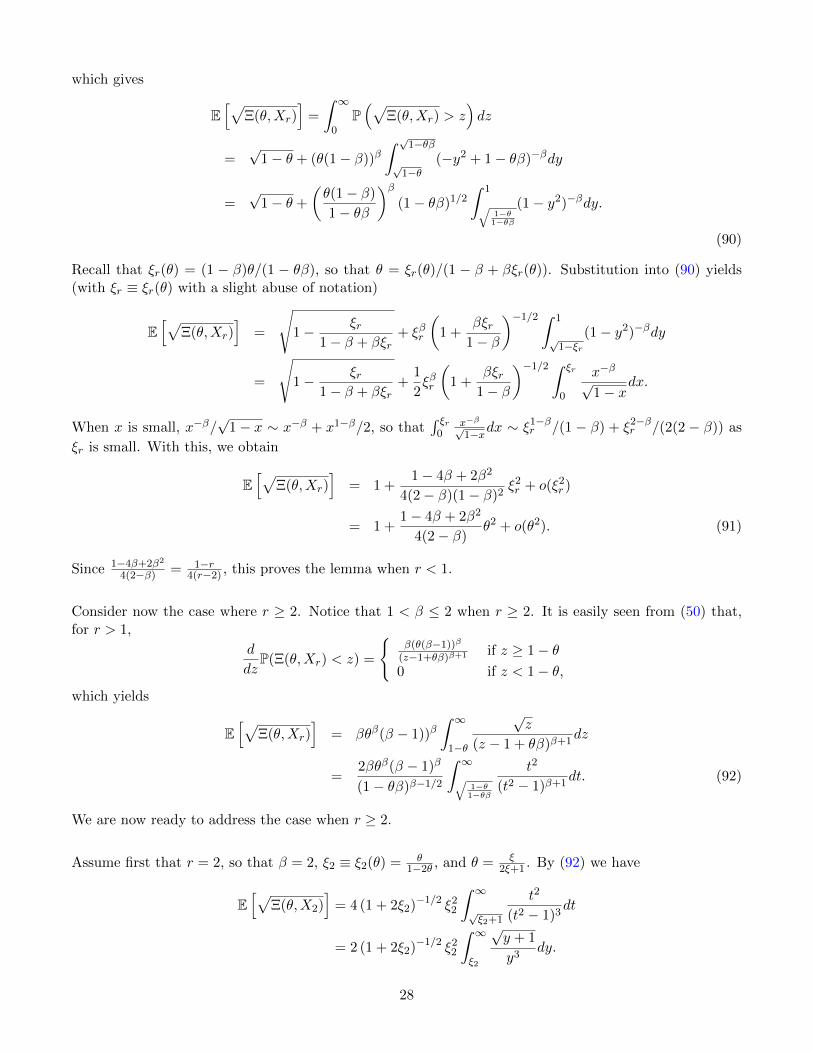
which gives
E[√
Ξ(θ,Xr)]
=
∫ ∞0
P(√
Ξ(θ,Xr) > z)dz
=√
1− θ + (θ(1− β))β∫ √1−θβ
√1−θ
(−y2 + 1− θβ)−βdy
=√
1− θ +
(θ(1− β)
1− θβ
)β(1− θβ)1/2
∫ 1√1−θ
1−θβ
(1− y2)−βdy.
(90)
Recall that ξr(θ) = (1 − β)θ/(1 − θβ), so that θ = ξr(θ)/(1 − β + βξr(θ)). Substitution into (90) yields(with ξr ≡ ξr(θ) with a slight abuse of notation)
E[√
Ξ(θ,Xr)]
=
√1− ξr
1− β + βξr+ ξβr
(1 +
βξr1− β
)−1/2 ∫ 1
√1−ξr
(1− y2)−βdy
=
√1− ξr
1− β + βξr+
1
2ξβr
(1 +
βξr1− β
)−1/2 ∫ ξr
0
x−β√1− x
dx.
When x is small, x−β/√
1− x ∼ x−β + x1−β/2, so that∫ ξr
0x−β√1−xdx ∼ ξ1−β
r /(1 − β) + ξ2−βr /(2(2 − β)) as
ξr is small. With this, we obtain
E[√
Ξ(θ,Xr)]
= 1 +1− 4β + 2β2
4(2− β)(1− β)2ξ2r + o(ξ2
r )
= 1 +1− 4β + 2β2
4(2− β)θ2 + o(θ2). (91)
Since 1−4β+2β2
4(2−β) = 1−r4(r−2) , this proves the lemma when r < 1.
Consider now the case where r ≥ 2. Notice that 1 < β ≤ 2 when r ≥ 2. It is easily seen from (50) that,for r > 1,
d
dzP(Ξ(θ,Xr) < z) =
β(θ(β−1))β
(z−1+θβ)β+1 if z ≥ 1− θ0 if z < 1− θ,
which yields
E[√
Ξ(θ,Xr)]
= βθβ(β − 1))β∫ ∞
1−θ
√z
(z − 1 + θβ)β+1dz
=2βθβ(β − 1)β
(1− θβ)β−1/2
∫ ∞√1−θ
1−θβ
t2
(t2 − 1)β+1dt. (92)
We are now ready to address the case when r ≥ 2.
Assume first that r = 2, so that β = 2, ξ2 ≡ ξ2(θ) = θ1−2θ , and θ = ξ
2ξ+1 . By (92) we have
E[√
Ξ(θ,X2)]
= 4 (1 + 2ξ2)−1/2 ξ22
∫ ∞√ξ2+1
t2
(t2 − 1)3dt
= 2 (1 + 2ξ2)−1/2 ξ22
∫ ∞ξ2
√y + 1
y3dy.
28
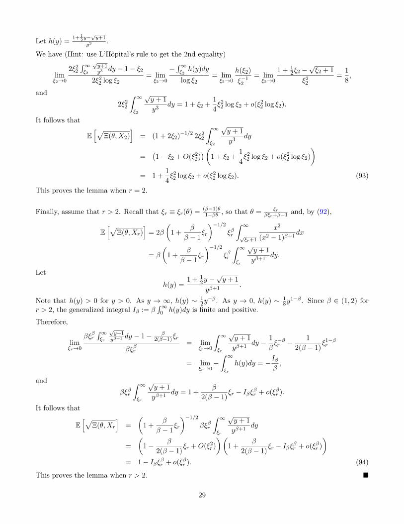
Let h(y) =1+ 1
2y−√y+1
y3 .
We have (Hint: use L’Hopital’s rule to get the 2nd equality)
limξ2→0
2ξ22
∫∞ξ2
√y+1y3 dy − 1− ξ2
2ξ22 log ξ2
= limξ2→0
−∫∞ξ2h(y)dy
log ξ2= lim
ξ2→0
h(ξ2)
ξ−12
= limξ2→0
1 + 12ξ2 −
√ξ2 + 1
ξ22
=1
8,
and
2ξ22
∫ ∞ξ2
√y + 1
y3dy = 1 + ξ2 +
1
4ξ2
2 log ξ2 + o(ξ22 log ξ2).
It follows that
E[√
Ξ(θ,X2)]
= (1 + 2ξ2)−1/2 2ξ22
∫ ∞ξ2
√y + 1
y3dy
=(1− ξ2 +O(ξ2
2))(
1 + ξ2 +1
4ξ2
2 log ξ2 + o(ξ22 log ξ2)
)= 1 +
1
4ξ2
2 log ξ2 + o(ξ22 log ξ2). (93)
This proves the lemma when r = 2.
Finally, assume that r > 2. Recall that ξr ≡ ξr(θ) = (β−1)θ1−βθ , so that θ = ξr
βξr+β−1 and, by (92),
E[√
Ξ(θ,Xr)]
= 2β
(1 +
β
β − 1ξr
)−1/2
ξβr
∫ ∞√ξr+1
x2
(x2 − 1)β+1dx
= β
(1 +
β
β − 1ξr
)−1/2
ξβr
∫ ∞ξr
√y + 1
yβ+1dy.
Let
h(y) =1 + 1
2y −√y + 1
yβ+1.
Note that h(y) > 0 for y > 0. As y → ∞, h(y) ∼ 12y−β. As y → 0, h(y) ∼ 1
8y1−β. Since β ∈ (1, 2) for
r > 2, the generalized integral Iβ := β∫∞
0 h(y)dy is finite and positive.
Therefore,
limξr→0
βξβr∫∞ξr
√y+1yβ+1 dy − 1− β
2(β−1)ξr
βξβr= lim
ξr→0
∫ ∞ξr
√y + 1
yβ+1dy − 1
βξ−βr − 1
2(β − 1)ξ1−βr
= limξr→0
−∫ ∞ξr
h(y)dy = −Iββ,
and
βξβr
∫ ∞ξr
√y + 1
yβ+1dy = 1 +
β
2(β − 1)ξr − Iβξβr + o(ξβr ).
It follows that
E[√
Ξ(θ,Xr
]=
(1 +
β
β − 1ξr
)−1/2
βξβr
∫ ∞ξr
√y + 1
yβ+1dy
=
(1− β
2(β − 1)ξr +O(ξ2
r )
)(1 +
β
2(β − 1)ξr − Iβξβr + o(ξβr )
)= 1− Iβξβr + o(ξβr ). (94)
This proves the lemma when r > 2.
29

F Appendix
Lemma F.1.limnDn = 0, (95)
where Dn is defined in (61).
Proof. Fix ε > 0. Since ∆2(z) = o(z2 log z) there exists zε > 0 such that for all 0 < z < zε,∣∣∣ ∆2(z)z2 log z
∣∣∣ < ε.
Since for all n such that δφ(n)−2δ < zε we have ξ2 = δe−µv
φ(n)−2δe−µv < zε for all v ≥ 0 (Hint: the mapping
v → ξ2 is nonincreasing in [0,∞) and ξ2 = δφ(n)−2δ when v = 0), we conclude that for n large enough,
supv≥0
∣∣∣∣ ∆2(ξ2)
ξ22 log ξ2
∣∣∣∣ < ε. (96)
Hence, for n large enough,
|Dn| ≤(
1
4+ ε
)∫ ∞0
λe−(λ+2µ)v
∣∣∣∣ log ξ2
(φ(n)− 2δe−µv)2
∣∣∣∣ dv=
(1
4+ ε
)∫ ∞0
λe−(λ+2µ)v
∣∣∣∣ log(φ(n)− 2δe−µv) + µv − log δ
(φ(n)− 2δe−µv)2
∣∣∣∣ dv. (97)
For n large enough
an(v) :=
∣∣∣∣ log(φ(n)− 2δe−µv) + µv − log δ
(φ(n)− 2δe−µv)2
∣∣∣∣ (98)
≤ µv − log δ +| log(φ(n)− 2δe−µv)|
(φ(n)− 2δe−µv)2
for all v ≥ 0. It is easy to check that for all n such that φ(n) > 2δ+√e, the mapping v → log(φ(n)−2−δe−λv)
(φ(n)−2δe−λv)2
is non-decreasing in [0,∞). Therefore, for all n such that φ(n) > 2δ +√e,
log(φ(n)− 2δe−µv)
(φ(n)− 2δe−µv)2≤ log(φ(n)− 2δ)
(φ(n)− 2δ)2for all v ≥ 0.
This shows that for all n such that φ(n) > 2δ +√e [Hint: φ(n) − 2δe−λv > 1 for all v ≥ 0 when
φ(n) > 2δ +√e]
| log(φ(n)− 2δe−µv)|(φ(n)− 2δe−µv)2
=log(φ(n)− 2δe−µv)
(φ(n)− 2δe−µv)2
≤ log(φ(n)− 2δ)
(φ(n)− 2δ)2∀v ≥ 0. (99)
We conclude from (98) and (99) that for n large enough [Hint: for n large enough, log(φ(n)− 2δ)/(φ(n)−2δ)2) < 1 since log t/t2 → 0 as t→∞ and φ(n)→∞ as n→∞]
0 ≤ an(v) ≤ µv + 1− log δ for all v ≥ 0.
Since for every v ≥ 0, an(v)→ 0 as n→∞ (cf. (98)), and∫ ∞0
λe−(λ+2µ)v(µv + 1− log δ)dv =λµ
(λ+ 2µ)2+λ(1− log δ)
λ+ 2µ<∞,
30
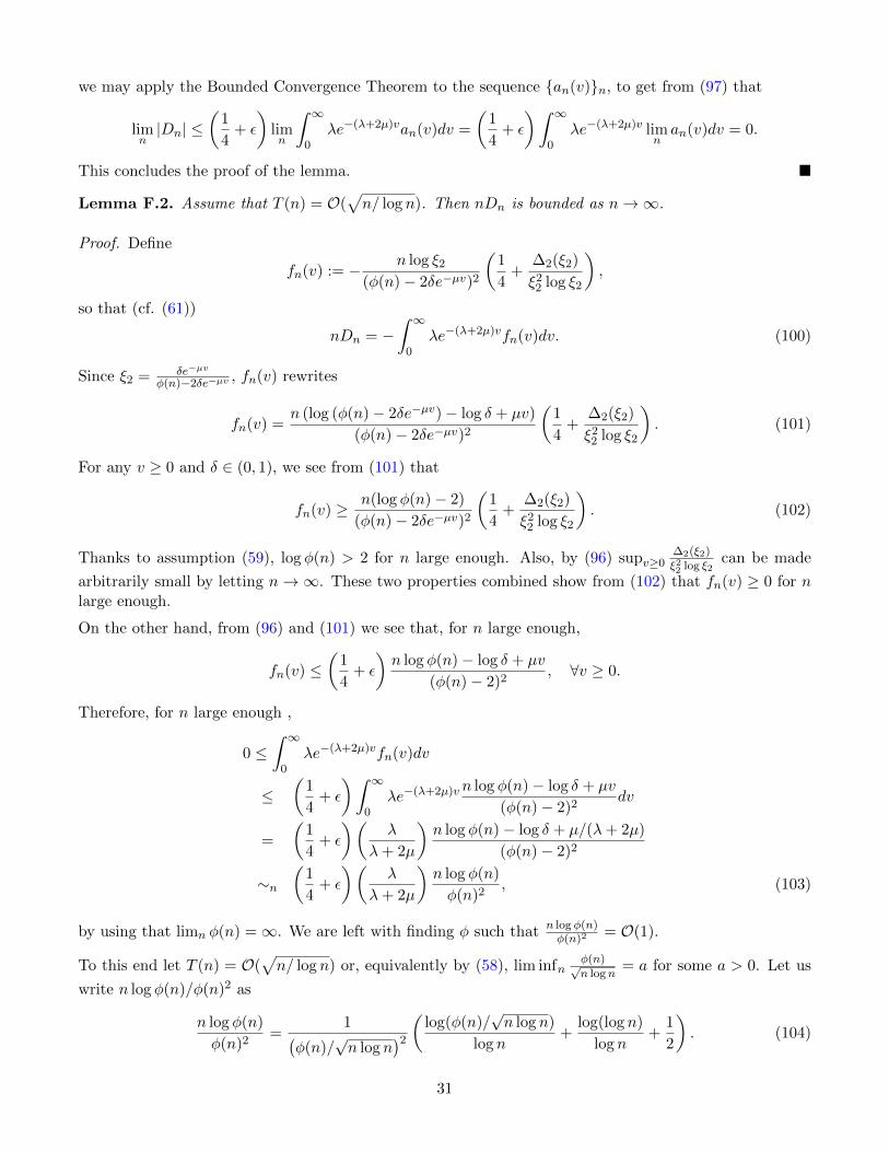
we may apply the Bounded Convergence Theorem to the sequence an(v)n, to get from (97) that
limn|Dn| ≤
(1
4+ ε
)limn
∫ ∞0
λe−(λ+2µ)van(v)dv =
(1
4+ ε
)∫ ∞0
λe−(λ+2µ)v limnan(v)dv = 0.
This concludes the proof of the lemma.
Lemma F.2. Assume that T (n) = O(√n/ log n). Then nDn is bounded as n→∞.
Proof. Define
fn(v) := − n log ξ2
(φ(n)− 2δe−µv)2
(1
4+
∆2(ξ2)
ξ22 log ξ2
),
so that (cf. (61))
nDn = −∫ ∞
0λe−(λ+2µ)vfn(v)dv. (100)
Since ξ2 = δe−µv
φ(n)−2δe−µv , fn(v) rewrites
fn(v) =n (log (φ(n)− 2δe−µv)− log δ + µv)
(φ(n)− 2δe−µv)2
(1
4+
∆2(ξ2)
ξ22 log ξ2
). (101)
For any v ≥ 0 and δ ∈ (0, 1), we see from (101) that
fn(v) ≥ n(log φ(n)− 2)
(φ(n)− 2δe−µv)2
(1
4+
∆2(ξ2)
ξ22 log ξ2
). (102)
Thanks to assumption (59), log φ(n) > 2 for n large enough. Also, by (96) supv≥0∆2(ξ2)ξ22 log ξ2
can be made
arbitrarily small by letting n→∞. These two properties combined show from (102) that fn(v) ≥ 0 for nlarge enough.
On the other hand, from (96) and (101) we see that, for n large enough,
fn(v) ≤(
1
4+ ε
)n log φ(n)− log δ + µv
(φ(n)− 2)2, ∀v ≥ 0.
Therefore, for n large enough ,
0 ≤∫ ∞
0λe−(λ+2µ)vfn(v)dv
≤(
1
4+ ε
)∫ ∞0
λe−(λ+2µ)v n log φ(n)− log δ + µv
(φ(n)− 2)2dv
=
(1
4+ ε
)(λ
λ+ 2µ
)n log φ(n)− log δ + µ/(λ+ 2µ)
(φ(n)− 2)2
∼n(
1
4+ ε
)(λ
λ+ 2µ
)n log φ(n)
φ(n)2, (103)
by using that limn φ(n) =∞. We are left with finding φ such that n log φ(n)φ(n)2 = O(1).
To this end let T (n) = O(√n/ log n) or, equivalently by (58), lim infn
φ(n)√n logn
= a for some a > 0. Let us
write n log φ(n)/φ(n)2 as
n log φ(n)
φ(n)2=
1(φ(n)/
√n log n
)2 ( log(φ(n)/√n log n)
log n+
log(log n)
log n+
1
2
). (104)
31
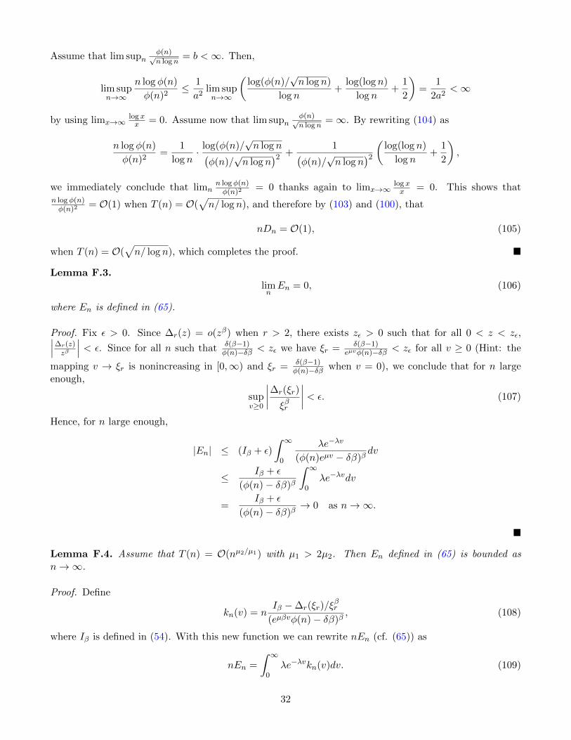
Assume that lim supnφ(n)√n logn
= b <∞. Then,
lim supn→∞
n log φ(n)
φ(n)2≤ 1
a2lim supn→∞
(log(φ(n)/
√n log n)
log n+
log(log n)
log n+
1
2
)=
1
2a2<∞
by using limx→∞log xx = 0. Assume now that lim supn
φ(n)√n logn
=∞. By rewriting (104) as
n log φ(n)
φ(n)2=
1
log n· log(φ(n)/
√n log n(
φ(n)/√n log n
)2 +1(
φ(n)/√n log n
)2 ( log(log n)
log n+
1
2
),
we immediately conclude that limnn log φ(n)φ(n)2 = 0 thanks again to limx→∞
log xx = 0. This shows that
n log φ(n)φ(n)2 = O(1) when T (n) = O(
√n/ log n), and therefore by (103) and (100), that
nDn = O(1), (105)
when T (n) = O(√n/ log n), which completes the proof.
Lemma F.3.limnEn = 0, (106)
where En is defined in (65).
Proof. Fix ε > 0. Since ∆r(z) = o(zβ) when r > 2, there exists zε > 0 such that for all 0 < z < zε,∣∣∣∆r(z)zβ
∣∣∣ < ε. Since for all n such that δ(β−1)φ(n)−δβ < zε we have ξr = δ(β−1)
eµvφ(n)−δβ < zε for all v ≥ 0 (Hint: the
mapping v → ξr is nonincreasing in [0,∞) and ξr = δ(β−1)φ(n)−δβ when v = 0), we conclude that for n large
enough,
supv≥0
∣∣∣∣∆r(ξr)
ξβr
∣∣∣∣ < ε. (107)
Hence, for n large enough,
|En| ≤ (Iβ + ε)
∫ ∞0
λe−λv
(φ(n)eµv − δβ)βdv
≤Iβ + ε
(φ(n)− δβ)β
∫ ∞0
λe−λvdv
=Iβ + ε
(φ(n)− δβ)β→ 0 as n→∞.
Lemma F.4. Assume that T (n) = O(nµ2/µ1) with µ1 > 2µ2. Then En defined in (65) is bounded asn→∞.
Proof. Define
kn(v) = nIβ −∆r(ξr)/ξ
βr
(eµβvφ(n)− δβ)β, (108)
where Iβ is defined in (54). With this new function we can rewrite nEn (cf. (65)) as
nEn =
∫ ∞0
λe−λvkn(v)dv. (109)
32
Notice that
kn(v) =Iβ −∆r(ξr)/ξ
βr
(eµβvφ(n)/n1/β − δβ/n1/β)β
≤Iβ −∆r(ξr)/ξ
βr
(φ(n)/n1/β − δβ/n1/β)β, (110)
for all n ≥ 1 and v ≥ 0. Recall that Iβ > 0. Let ε < Iβ in (107). From (110) we see that for n large enough
0 ≤ kn(v) ≤Iβ + ε
(φ(n)/n1/β − δβ/n1/β)βfor all v ≥ 0. (111)
Recall that β = rr−1 yielding r = β
β−1 . Assume that T (n) = δnφ(n) = O(n1/r) for δ ∈ (0, 1), or equivalently
lim infn
φ(n)
n1/β= b
for some b > 0. From (111) we obtain
0 ≤ lim supn
∫ ∞0
λe−λvkn(v)dv
≤ lim supn
Iβ + ε
(φ(n)/n1/β − δβ/n1/β)β
=Iβ + ε
(lim infn φ(n)/n1/β)β=Iβ + ε
bβ. (112)
This shows that nEn ∈ O(1).
G Appendix
Lemma G.1. For any θ ∈ [0, 1], r′ ≥ r,
E[√
Ξ(θ,Xr′)]≤ E
[√Ξ(θ,Xr)
].
Proof. Fix θ ∈ [0, 1]. When r′ ≥ r then Xr′ ≤st Xr, which in turn implies that Ξ(θ,Xr′) ≤st Ξ(θ,Xr) asthe mapping x→ Ξ(θ, x) in (50) is nondecreasing in [0,∞),
Therefore,
E[√
Ξ(θ,Xr′)]≤ E
[√Ξ(θ,Xr)
],
as the mapping x→√x is nondecreasing in [0,∞).
H Appendix: Proof of Proposition 5.5
Recall that under the IEBP policy the system behaves as an M/G/1 queue with an exceptional first job ineach busy period. The service times of first jobs in busy periods have pdf f1 and the service times of theother jobs have pdf g1. The numbers of jobs served in different busy periods are iid rvs, characterized by therandom variable M , so that the expected number of Willie jobs served during n W-BPs is TW (n) = nE[M ].
33
Let us calculate E[M ]. To this end, introduce GM (z) = E[zM ], |z| ≤ 1, the generating function of thenumber of jobs served in a busy period. Recall (Section 4) that the reconstructed service times of the firstjob served in different busy periods are iid rvs, and let Y be a generic reconstructed service time. Letτ∗(s) = E[e−Y s] =
∫∞0 e−sxf1(x)dx be the LST of the reconstructed service time. Since the LTS of the
service times all the other Willie jobs in a W-BP is G∗1(s), we get from [4]
GM (z) = zτ∗(λ(1− d(z)), |z| ≤ 1, (113)
where d(z) is the root with the smallest modulus of the equation t = zG∗1(λ(1− t)).Noting that d(1) = 1 and d
d(z) |z=1 = 11−λ/µ1
, we obtain from (113)
E[M ] =1− λ/µ1 + λE[Y ]
1− λ/µ1, (114)
provided that the stability condition λ/µ1 < 1 holds. It remains to find E[Y ]. For that, we will use the
identity E[Y ] = −dτ∗(s)ds |s=0. But before that we need to calculate τ∗(s).
When IEBP is enforced (or, equivalently, under H1) we know that Y has pdf f1 (see Section 4.2) .Multiplying both sides of (46) by g1(x) and using the definition of Z(q, x) in (35) along with (47) gives
f1(x) = (1− qp)g1(x) + q(g1 ∗ g2)(x),
where g2(x) is defined in (48). Therefore,
τ∗(s) =
∫ ∞0
e−sxf1(x)dx =
∫ ∞0
e−sx[(1− pq)g1(x) + q(g1 ∗ g2)(x)]dx
= G∗1(s)
(1− pq + q
∫ ∞0
e−stg2(t)dt
). (115)
Differentiating (115) with respect to s at s = 0 and using the identity2∫∞
0 g2(t)dt = p yields
E[Y ] =1− pqµ1
+q
µ1
∫ ∞0
g2(t)dt+ q
∫ ∞0
tg2(t)dt
=1
µ1+ q
∫ ∞0
tg2(t)dt,
By (114),
E[M ] =1
1− λ/µ1+
λq
1− λ/µ1
∫ ∞0
tg2(t)dt, (116)
and
TW (n) = nE[M ] =n
1− λ/µ1+
λqn
1− λ/µ1
∫ ∞0
tg2(t)dt. (117)
Now we upper bound the integral in (116) and (117). We have∫ ∞0
tg2(t)dt =
∫ ∞0
λe−λv∫ ∞
0tg2(v + t)dvdt
≤∫ ∞
0λe−λv
∫ ∞0
(t+ v)g2(v + t)dvdt
=
∫ ∞0
λe−λv∫ ∞v
ug2(u)dudv
2∫∞
0g2(t)dt =
∫∞0λe−λv
∫∞vg2(t)dtdv =
∫∞0λe−λv(1−G2(v))dv = 1−G∗2(λ) = p.
34
≤∫ ∞
0λe−λv
∫ ∞0
ug2(u)dudv =1
µ2.
Hence, E[M ] ≤ 1+qλ/µ2
1−λ/µ1and TW (n) ≤ n
(1+qλ/µ2
1−λ/µ1
). This shows the upper bound in (28). The lower bound
is trivial.
If g2(x) = µ2e−µ2x then from (48) and (4) we find p = λ
µ2+λ and g2(x) = λµ2
(λ+µ2)e−µ2x = pµ2e
−µ2x, which
yields (29).
35


