Embed Size (px)
Citation preview
Analytic solution for rotating flowand heat transfer analysis of a third-grade fluid
T. Hayat, T. Javed, and M. Sajid, Islamabad, Pakistan
Received February 16, 2006; revised December 9, 2006Published online: April 19, 2007 � Springer-Verlag 2007
Summary. The present work examines the flow of a third grade fluid and heat transfer analysis between
two stationary porous plates. The governing non-linear flow problem is solved analytically using ho-
motopy analysis method (HAM). After combining the solution for the velocity, the temperature profile is
determined for the constant surface temperature case. Graphs for the velocity and temperature profiles are
presented and discussed for various values of parameters entering the problem.
1 Introduction
In recent years, it has generally been recognized that in industrial applications non-Newtonian
fluids are more appropriate than Newtonian fluids. For instance, in certain polymer processing
applications, one deals with the flow of a non-Newtonian fluid over a moving surface. That
non-Newtonian fluids are finding increasing application in industry has given impetus to many
researchers. The heat transfer analysis further plays an important role during the handling and
processing of non-Newtonian fluids. The understanding of heat transfer in flows of non-
Newtonian fluids is of importance in many engineering applications such as the design of thrust
bearings and radial diffusers, transpiration cooling, drag reduction, thermal recovery of oil etc.
The governing equations for non-Newtonian fluids are much more complicated than the
Navier-Stokes equations. This difficulty is due to the fact that the flow equations of non-
Newtonian fluids are highly non-linear and are of higher order [1], [2] when compared to the
equations dealing with the flow of viscous fluids. Such non-linear fluids lead to boundary value
problems in which the order of differential equations exceeds the number of available boundary
conditions. Ever since the simplest models of viscoelastic fluids were introduced, the researchers
in rheology have been looking for the elusive boundary condition(s) associated with the vis-
coelastic parameter, but essentially without success. For details of this issue, the reader may be
referred to the studies [3]–[8]. To find analytic solutions of such equations is not an easy task.
Due to this fact, several authors [9]–[16] are now engaged in finding analytic solutions under
imposed restrictions. The simplest subclass of non-Newtonian fluids for which one can rea-
sonably hope to obtain an analytic solution is the second grade. But for steady unidirectional
flow the second grade fluid acts like a Newtonian fluid. Because of this reason, the fluid model
of third grade is important. The third grade fluid model even for the steady flow situation yields
a non-linear equation.
Acta Mechanica 191, 219–229 (2007)
DOI 10.1007/s00707-007-0451-y
Printed in The NetherlandsActa Mechanica
The analysis of the effect of rotation and magnetic field in fluid flows has been an active area
of research due to its geophysical and technological importance. It is well known that a number
of astronomical bodies (e.g., the Sun, Earth, Jupiter, magnetic stars, pulsars) possess fluid
interiors and (at least surface) magnetic fields. Changes in the rotation rate of such objects
suggest the possible importance of hydromagnetic spin-up. Extensive literature relevant to the
analytic solution of such flows is available for Newtonian fluids. But very little attention has
been given to the analytic solution of rotating flows for non-Newtonian fluids. The analytic
solutions concerning rotating flows of non-Newtonian fluids have been reported by Hayat et al.
[17]–[19] and Asghar et al. [20].
In all the above mentioned problems [9]–[20], the authors used the second grade, Maxwell
and Oldroyd-B fluid models and obtained the analytic solutions for various linear flow
problems. In the present analysis, our concern is to investigate the Poiseuille flow of a third
grade fluid in a rotating frame. In fact the aim of the present study is threefold. Firstly to
consider a third grade fluid which yields a non-linear flow problem. Secondly, to obtain an
analytic solution, and thirdly, to analyze the heat transfer characteristics. We have obtained
the solutions in series form for the velocity and temperature by means of HAM proposed by
Liao [21], [22]. The HAM has already been successfully applied by various authors [23]–[36]
for non-linear problems. The obtained solutions here are important not only as solutions of
fundamental fluid flows but also serve as accuracy checks for the numerical and asymptotical
solutions.
2 Formulation of the problem
Let us consider the steady flow of a third grade fluid bounded by two porous parallel plates at
z ¼ 0 and z ¼ d: The lower plate is subjected to a uniform suction W0 and the upper plate is
under the action of constant blowing W0: In the undisturbed state, both the fluid and plates are
in a state of rigid body rotation with the uniform angular velocity X about the z-axis normal to
the plates. The fluid is driven by a constant pressure gradient, and heat transfer is due to
constant temperature of the lower plate. Using the Cartesian coordinate system Oxyz; the
motion in this rotating frame is governed by the momentum equation, the continuity equation
and the energy equation as follows:
q
�dV
dtþ 2X� V þX� X� rð Þ
�¼ divr; ð1Þ
divV ¼ 0; ð2Þ
qcdT
dt¼ r:L� divq; ð3Þ
where q is the fluid density, c is the specific heat capacity, T is the temperature, L is the velocity
gradient, t is the time, q is the heat flux vector, r is the Cauchy stress tensor which for a
thermodynamic third grade fluid is [28]
r ¼ �pIþ lþ btrA21
� �A1 þ a1A2 þ a2A2
1; ð4Þ
in which p is the pressure, I is the identity tensor, l, a1; a2; and b are material constants. The
velocity field for the present flow is
V ¼ ½u zð Þ; v zð Þ; w zð Þ�; ð5Þ
220 T. Hayat et al.
which together with Eq. (2) gives w ¼ �W0 (W0 > 0 corresponds to the suction velocity and
W0 < 0 indicates blowing).
The equations (1), (3), (4) and (5) after using the non-dimensional variables
F� ¼ F
U0; z� ¼ z
d; b� ¼ bU2
0
tqd2; W�
0 ¼W0d
t; X� ¼ Xd2
t;
a�1 ¼a1
qd2; C ¼ d2
qtU20
@p
@xþ i
@p
@y
� �; hðz�Þ ¼ T � Td
T0 � Td
;
ð6Þ
give
�W0dF
dzþ 2iXF ¼ �Cþ d2F
dz2� a1W0
d3F
dz3þ 2b
d
dz
dF
dz
� �2d �F
dz
" #; ð7Þ
d2hdz2þ Pr W0
dhdz� Ec
a1W0
2
d
dz
dF
dz
d �F
dz
� �� 2b
dF
dz
d �F
dz
� �2
�dF
dz
d �F
dz
( )" #¼ 0; ð8Þ
where F ¼ uþ iv; �F ¼ u� iv; the Prandtl number Pr ¼ lcp=k; the Eckert number Ec ¼U2
0=cpðT0 � TdÞ; t is the kinematic viscosity and asterisks have been suppressed for brevity.
The non-dimensional boundary conditions are
F 0ð Þ ¼ 0; F 1ð Þ ¼ 0; h 0ð Þ ¼ 1; h 1ð Þ ¼ 0: ð9Þ
3 HAM solution for F(z)
Here the initial approximation F0ðzÞ and the auxiliary linear operator L are
F0 zð Þ ¼ C
2z2 � z� �
; ð10Þ
L Fð Þ ¼ F00 � C; L Cz2 þ C1zþ C2
� �¼ 0; ð11Þ
where C is the constant pressure gradient and C1 and C2 are arbitrary constants. Using the same
procedure as in [30], the HAM solution for F is given by
F zð Þ ¼ limM!1
X4Mþ2
n¼1
X4Mþ1
m¼n�1
am;nzn
!" #; ð12Þ
where for m � 1, 0 � n � 4mþ 2
am;1 ¼ vmv4m�1am�1;1 þC
2�X4mþ2
n¼0
Cm;n
nþ 1ð Þ nþ 2ð Þ ; ð13Þ
am;2 ¼ vmv4m�2am�1;2 �C
2þ Cm;0
2; ð14Þ
am;n ¼ vmv4m�nam�1;n þCm;n�2
n n� 1ð Þ ; 3 � n � 4mþ 2; ð15Þ
vm ¼0; m � 1;
1; m > 1;
(ð16Þ
Analytic solution for rotating flow 221
Cm;n ¼
�hC 1� vmð Þ �W0bm�1;0 þ 2iXam�1;0
þ a1W0 � 1ð Þcm�1;0 � 2b 2dm;0 þ Dm;0
� �24
35; n ¼ 0;
�hv2m�nþ1 �W0bm�1;n þ 2iXam�1;n þ a1W0 � 1ð Þcm�1;n
� �
2b 2dm;n þ Dm;n
� �24
35; n � 1;
8>>>>>>><>>>>>>>:
ð17Þ
dqm;n ¼
Xm�1
k¼0
Xk
l¼0
Xminfn;2kþ2g
p¼maxf0;n�2mþ2kþ1g
Xminfp;2lþ1g
s¼maxf0;p�2kþ2l�1g
�bl;sbk�l;p�scm�1�k;n�p; ð18Þ
Dqm;n ¼
Xm�1
k¼0
Xk
l¼0
Xminfn;2kþ2g
p¼maxf0;n�2mþ2kþ1g
Xminfp;2lþ1g
s¼maxf0;p�2kþ2l�1g�cl;sbk�l;p�sbm�1�k;n�p; ð19Þ
bm;n ¼ nþ 1ð Þam;nþ1; cm;n ¼ nþ 1ð Þbm;nþ1; ð20Þ
a0;0 ¼ 0; a0;1 ¼ �C
2; a0;2 ¼
C
2: ð21Þ
4 HAM solution for hðzÞ
The initial guess approximation and the auxiliary linear operator are
h0 zð Þ ¼ 1� z; ð22Þ
L hð Þ ¼ h00; L C3zþ C4ð Þ ¼ 0; ð23Þ
where C3 and C4 are arbitrary constants.
Using the same methodology of solution as in the previous Section we have
h zð Þ ¼ limM!1
X4Mþ4
n¼1
X4Mþ3
m¼n�1
am;nzn
!" #; ð24Þ
where for m � 1, 0 � n � 4mþ 4 we have
am;0 ¼ vmv4mþ2am�1;0; ð25Þ
am;1 ¼ vmv4mþ1am�1;1 �X4mþ4
n¼0
C1m;n
nþ 1ð Þ nþ 2ð Þ ; ð26Þ
am;n ¼ vmv4m�nþ2am�1;n þC1m;n�2
n n� 1ð Þ ; 2 � n � 4mþ 2; ð27Þ
C1m;n ¼ �h1 v4m�nþ2
em�1;n þ Pr W0dm�1;n
�Pr Eca1W0
2Dm;n þ bm;n
� �� cm;n
� �8<:
9=;� 2 Pr Ecbdm;n
24
35; ð28Þ
Dm;n ¼Xm�1
k¼0
Xminfn;4kþ2g
s¼maxf0;n�4ðm�kÞþ2gcm�1�k;n�s
�bk;s; ð29Þ
222 T. Hayat et al.
bm;n ¼Xm�1
k¼0
Xminfn;4kþ2g
s¼maxf0;n�4ðm�kÞþ2gbm�1�k;n�s�ck;s; ð30Þ
cm;n ¼Xm�1
k¼0
Xminfn;4kþ2g
s¼maxf0;n�4ðm�kÞþ2gbm�1�k;n�s
�bk;s; ð31Þ
q¢¢ (
0)
0.3 15th order app
0.2
0.25
0.15
0.05
0.1
–2 –1.5 –0.5 0–1
W Pr Ca= 2, = –0.35,0 E = 0.1,c = 1,1 b = = =0.1,0.1,= 0.1, 0.1, Wh
h1
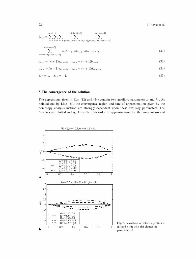
Fig. 2. �h1-Curve of temperatureprofile h for the 15th order of
approximation
15th order app.
15th order app.
W Ca= 2,
–1.4 –1.2 –0.8 –0.6 –0.4 –0.2 0–1
–1.4 –1.2 –0.8 –0.6 –0.4 –0.2 0–1
0 = 1, 1,1 b = = =0.1, 0.1, W
W Ca= 2,0 = 1, 1,1 b = = =0.1, 0.1, W
u¢ (0
)v¢
(0)
4
2
–2
–1
–2
–1.5
–2.5
–4
–0.5
0
0
h
h
a
b
Fig. 1. �h-Curves of velocity profiles u
(a) and v (b) for the 15th order ofapproximation
Analytic solution for rotating flow 223
dm;n ¼Xm�1
k¼0
Xk
l¼0
Xl
i¼0
Xminfn;4kþ6g
q¼maxf0;n�4ðm�kÞþ2g
Xminfq;4lþ4g
p¼maxf0;q�4ðk�lÞ�4g
Xminfp;4iþ2g
r¼maxf0;p�4ðl�iÞ�2g
�bi;r�bl�i;p�rbk�l;q�pbm�1�k;n�q; ð32Þ
bm;n ¼ nþ 1ð Þam;nþ1; cm;n ¼ nþ 1ð Þbm;nþ1; ð33Þ
dm;n ¼ nþ 1ð Þam;nþ1; em;n ¼ nþ 1ð Þdm;nþ1; ð34Þ
a0;0 ¼ 1; a0;1 ¼ �1: ð35Þ
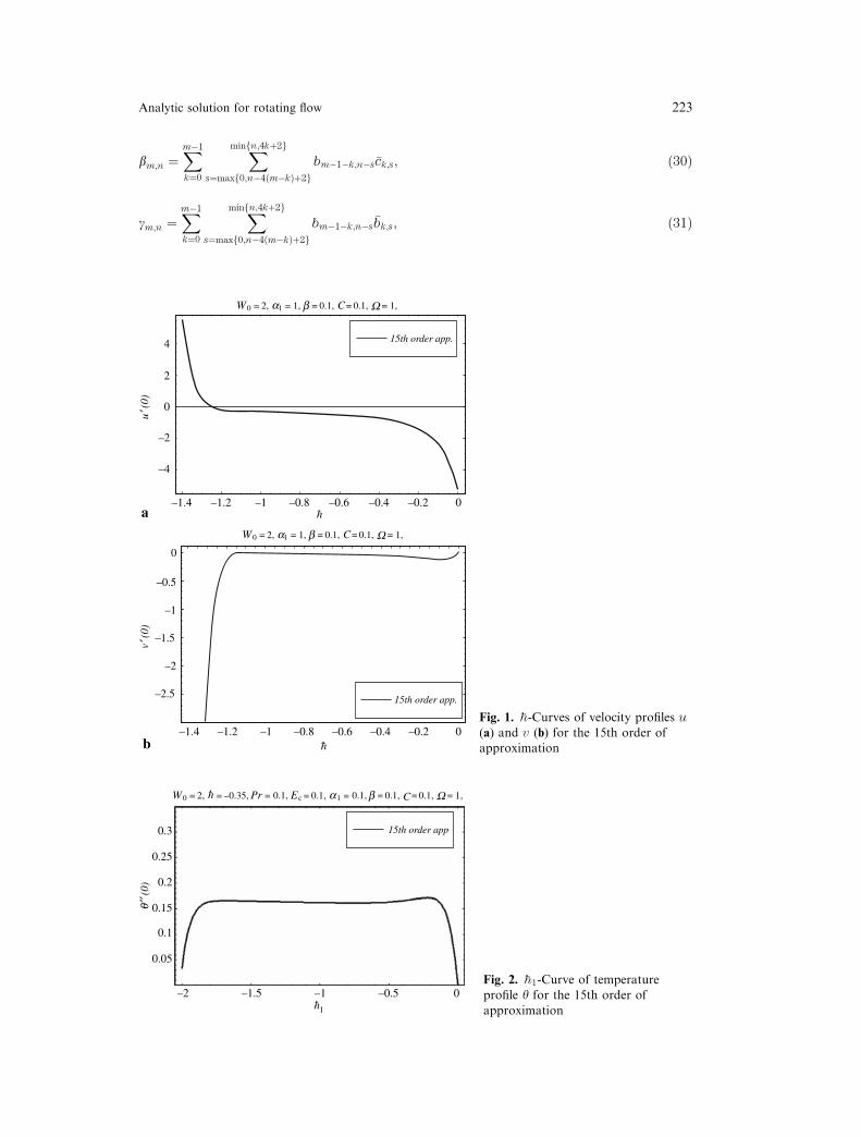
5 The convergence of the solution
The expressions given in Eqs. (12) and (24) contain two auxiliary parameters �h and �h1: As
pointed out by Liao [21], the convergence region and rate of approximation given by the
homotopy analysis method are strongly dependent upon these auxiliary parameters. The
�h-curves are plotted in Fig. 1 for the 15th order of approximation for the non-dimensional
b = 0.1,a =1 0.1,W = 2, = –0.5,
= 0.0, = 0.0= 0.1,
= 0.1,= 1.5,
= 1.5,
= 0.1= 0.1= –0.1= –0.1
0 h
0 0.2 0.4 0.6 0.8 1z
u(z)
4
2
2
1.5
0.5
–0.5
–1
–1.5
0
0 0.2 0.4 0.6 0.8 1
1
–2
–4
0
W CCCCC
WWWW
= 0.0, = 0.0= 0.5,= 1.0,= 0.5,= 1.0,
= 0.1= 0.1= –0.1= –0.1
W CCCCC
WWWW
a
b
b = 0.1,a =1 0.1,W = 2, = –0.5,0 h
v(z)
z
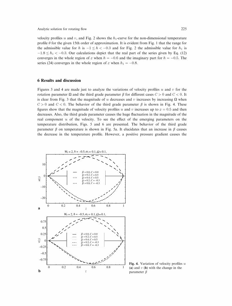
Fig. 3. Variation of velocity profiles u
(a) and v (b) with the change in
parameter X
224 T. Hayat et al.
velocity profiles u and v, and Fig. 2 shows the �h1-curve for the non-dimensional temperature
profile h for the given 15th order of approximation. It is evident from Fig. 1 that the range for
the admissible value for �h is �1 � �h < �0:3 and for Fig. 2 the admissible value for �h1 is
�1:8 � �h1 < �0:3: Our calculations depict that the real part of the series given by Eq. (12)
converges in the whole region of z when �h ¼ �0:6 and the imaginary part for �h ¼ �0:5: The
series (24) converges in the whole region of z when �h1 ¼ �0:8:
6 Results and discussion
Figures 3 and 4 are made just to analyze the variations of velocity profiles u and v for the
rotation parameter X and the third grade parameter b for different cases C > 0 and C < 0. It
is clear from Fig. 3 that the magnitude of u decreases and v increases by increasing X when
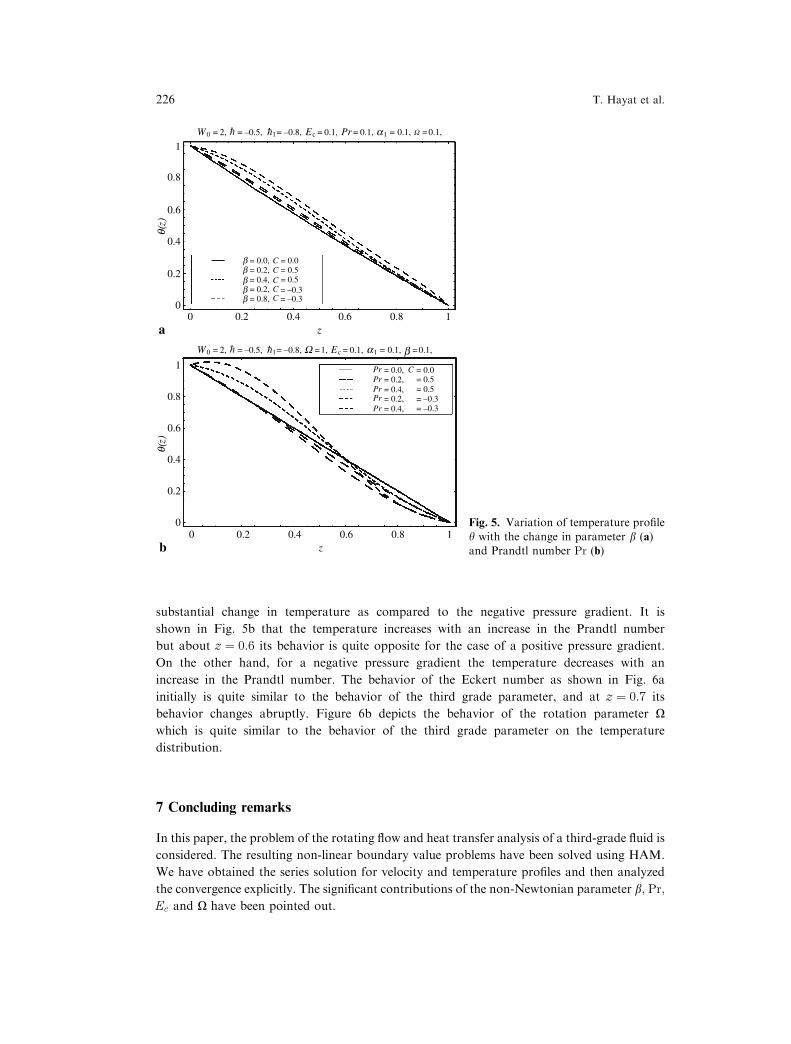
C > 0 and C < 0. The behavior of the third grade parameter b is shown in Fig. 4. These
figures show that the magnitude of velocity profiles u and v increases up to z ¼ 0:5 and then
decreases. Also, the third grade parameter causes the huge fluctuation in the magnitude of the
real component u of the velocity. To see the effect of the emerging parameters on the
temperature distribution, Figs. 5 and 6 are presented. The behavior of the third grade
parameter b on temperature is shown in Fig. 5a. It elucidates that an increase in b causes
the decrease in the temperature profile. However, a positive pressure gradient causes the
z
W = 0.1,a =1 0.1,W = 2, = –0.5,0 h
10
–10
–20
0
0 0.2 0.4 0.6 0.8 1
u(z)
= 0.0,= 0.2,
= 0.0= 0.5= 0.5= –0.3= –0.3
bb
= 0.4,b= 0.2,b= 0.8,b
CCCCC
= 0.0,= 0.2,
= 0.0= 0.5= 0.5= –0.3= –0.3
bb
= 0.4,b= 0.2,b= 0.8,b
CCCCC
a
W = 0.1,a =1 0.1,W = 2, = –0.5,0 h
z0 0.2 0.4 0.6 0.8 1
b
v(z) 0
0.25
–0.25
–0.5
0.75
–0.75
0.5
Fig. 4. Variation of velocity profiles u
(a) and v (b) with the change in the
parameter b
Analytic solution for rotating flow 225
substantial change in temperature as compared to the negative pressure gradient. It is
shown in Fig. 5b that the temperature increases with an increase in the Prandtl number
but about z ¼ 0:6 its behavior is quite opposite for the case of a positive pressure gradient.
On the other hand, for a negative pressure gradient the temperature decreases with an
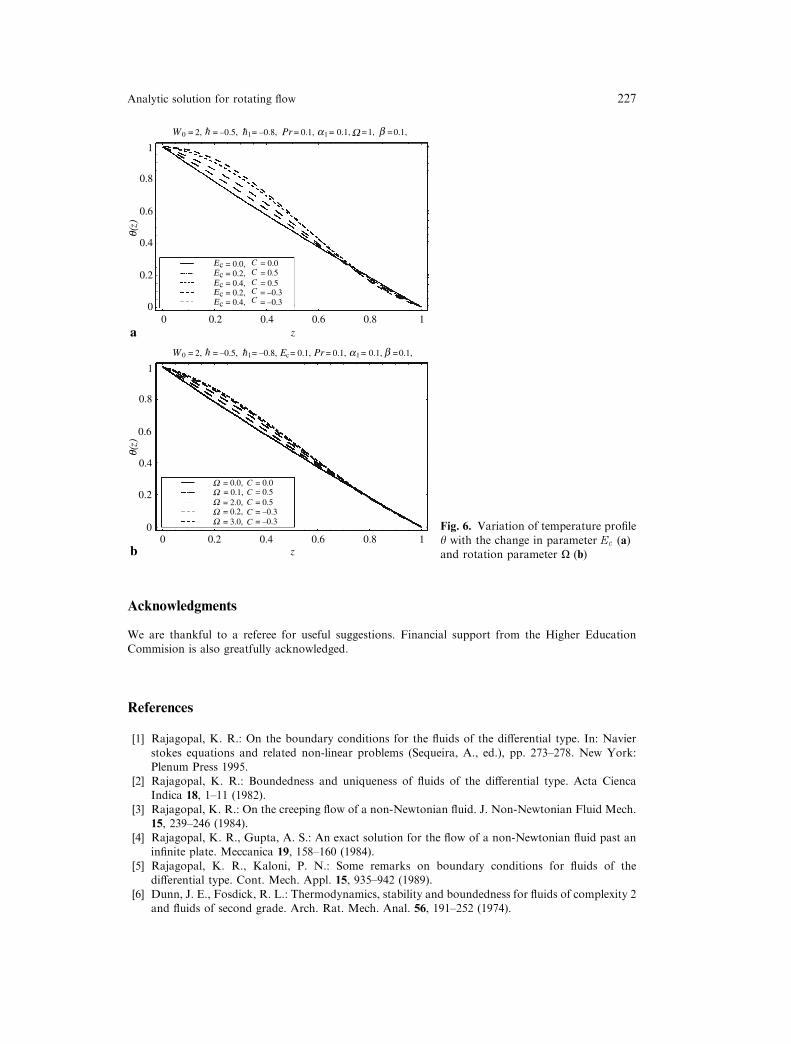
increase in the Prandtl number. The behavior of the Eckert number as shown in Fig. 6a
initially is quite similar to the behavior of the third grade parameter, and at z ¼ 0:7 its
behavior changes abruptly. Figure 6b depicts the behavior of the rotation parameter Xwhich is quite similar to the behavior of the third grade parameter on the temperature
distribution.
7 Concluding remarks
In this paper, the problem of the rotating flow and heat transfer analysis of a third-grade fluid is
considered. The resulting non-linear boundary value problems have been solved using HAM.
We have obtained the series solution for velocity and temperature profiles and then analyzed
the convergence explicitly. The significant contributions of the non-Newtonian parameter b; Pr;
Ec and X have been pointed out.
W h a= 2, = –0.5, –0.8,0 E = 0.1,c Pr = 0.1,1 =1 =0.1,= 0.1,Wh
W h a= 2, = –0.5, –0.8,0 E = 0.1,c 1 =1 =0.1,= 0.1,b=1,Wh
1
0.8
0.6
q(z)
0.4
0.2
0
1
0.8
0.6
q(z)
0.4
0.2
0
z0 0.2 0.4 0.6 0.8 1
z0 0.2 0.4 0.6 0.8 1
= 0.0, = 0.0b C
= 0.0,= 0.2,= 0.4,= 0.2,= 0.4,
= 0.0= 0.5= 0.5= –0.3= –0.3
PrPrPrPrPr
C
= 0.2,
= 0.2,= 0.8,
= 0.4,= 0.5= 0.5= –0.3= –0.3
bbbb
CCCC
a
b
Fig. 5. Variation of temperature profile
h with the change in parameter b (a)and Prandtl number Pr (b)
226 T. Hayat et al.
Acknowledgments
We are thankful to a referee for useful suggestions. Financial support from the Higher Education
Commision is also greatfully acknowledged.
References
[1] Rajagopal, K. R.: On the boundary conditions for the fluids of the differential type. In: Navier
stokes equations and related non-linear problems (Sequeira, A., ed.), pp. 273–278. New York:Plenum Press 1995.
[2] Rajagopal, K. R.: Boundedness and uniqueness of fluids of the differential type. Acta CiencaIndica 18, 1–11 (1982).
[3] Rajagopal, K. R.: On the creeping flow of a non-Newtonian fluid. J. Non-Newtonian Fluid Mech.15, 239–246 (1984).
[4] Rajagopal, K. R., Gupta, A. S.: An exact solution for the flow of a non-Newtonian fluid past aninfinite plate. Meccanica 19, 158–160 (1984).
[5] Rajagopal, K. R., Kaloni, P. N.: Some remarks on boundary conditions for fluids of thedifferential type. Cont. Mech. Appl. 15, 935–942 (1989).
[6] Dunn, J. E., Fosdick, R. L.: Thermodynamics, stability and boundedness for fluids of complexity 2and fluids of second grade. Arch. Rat. Mech. Anal. 56, 191–252 (1974).
W h a= 2, = –0.5, –0.8,0 Pr = 0.1,1 =1 =0.1,= 1,W =0.1,bh
W h a= 2, = –0.5, –0.8,0 PrE = 0.1,1 =1 0.1,= 0.1,c = =0.1,bh
z0 0.2 0.4 0.6 0.8 1
z0 0.2 0.4 0.6 0.8 1
1
0.8
0.6
q(z)
q(z)
0.4
0.2
0
1
0.8
0.6
0.4
0.2
0
a
b
= 0.0,
= 2.0,
= 3.0,= 0.2,
= 0.1,= 0.0= 0.5= 0.5= –0.3= –0.3
WWWWW
CCCCC
= 0.0, = 0.0EcEcEcEcEc
C= 0.2,
= 0.2,= 0.4,
= 0.4,= 0.5= 0.5= –0.3= –0.3
CCCC
Fig. 6. Variation of temperature profile
h with the change in parameter Ec (a)and rotation parameter X (b)
Analytic solution for rotating flow 227
[7] Girault, V., Scott, L. R.: Analysis of a two dimensional grade-two fluid model with a tangential
boundary condition. J. Math. Pure. Appl. 78, 981–1011 (1999).[8] Cortell, R.: A note on flow and heat transfer of a viscoelastic fluid over a stretching sheet. Int. J.
Non-Linear Mech. 41, 78–85 (2006).[9] Rajagopal, K. R.: A note on unsteady unidirectional flows of a non-Newtonian fluid. Int. J. Non-
Linear Mech. 17, 369–373 (1982).[10] Hayat, T., Asghar, S., Siddiqui, A. M.: Periodic unsteady flows of a non-Newtonian fluid. Acta
Mech. 131, 169–175 (1998).[11] Khan, M., Nadeem, S., Hayat, T., Siddiqui, A. M.: Unsteady motions of a generalized second
grade fluid. Math. Comput. Model. 41, 629–637 (2005).[12] Hayat, T., Nadeem, S., Asghar, S.: Periodic unidirectional flows of a viscoelastic fluid with the
fractional Maxwell model. Appl. Math. Comput. 151, 153–161 (2004).[13] Fetecau, C., Zierep, J.: Decay of a potential vortex and propagation of a heat wave in a second
grade fluid. Int. J. Non-Linear Mech. 37, 1051–1056 (2002).[14] Fetecau, C., Zierep, J.: On a class of exact solutions for the equations of motion of a second grade
fluid. Acta Mech. 150, 135–138 (2001).[15] Tan, W. C., Pan, W., Xu, M.: A note on unsteady flow of viscoelastic fluid with the fractional
Maxwell model between two parallel plates. Int. J. Non-Linear Mech. 38, 615–620 (2003).[16] Chen, C. I., Chen, C. K., Yang, Y. T.: Unsteady unidirectional flow of an Oldroyd-B fluid in a
circular duct with different given volume flow rate conditions. Int. J. Heat Mass Transf. 40, 203–209 (2004).
[17] Hayat, T., Wang, Y., Hutter, K.: Hall effects on the unsteady hydromagnetic oscillatory flow of asecond grade fluid. Int. J. Non-Linear Mech. 39, 1027–1031 (2004).
[18] Hayat, T., Nadeen, S., Siddiqui, A. M., Asghar, S.: An oscillatory hydromagnetic non-Newtonianflow in a rotating system. Appl. Math. Lett. 17, 609–614 (2004).
[19] Hayat, T., Hutter, K., Asghar, S., Siddiqui, A. M.: MHD flows of an Oldroyd-B fluid. Math.Comput. Model. 36, 985–995 (2002).
[20] Asghar, S., Parveen, S., Hanif, S., Siddiqui, A. M., Hayat, T.: Hall effect on the unsteadyhydromagnetic flows of an Oldroyd-B fluid. Int. J. Engng. Sci. 41, 609–619 (2003).
[21] Liao, S. J.: Beyond perturbation: Introduction to homotopy analysis method. Boca Raton:Chapman & Hall/CRC Press 2003.
[22] Liao, S. J.: On the homotopy analysis method for nonlinear problems. Appl. Math. Comput. 147,499–513 (2004).
[23] Liao, S. J.: A uniformly valid analytic solution of 2D viscous flow past a semi-infinite flat plate.J. Fluid Mech. 385, 101–128 (1999).
[24] Liao, S. J., Campo, A.: Analytic solutions of the temperature distribution in Blasius viscous flowproblems. J. Fluid Mech. 453, 411–425 (2002).
[25] Liao, S. J.: On the analytic solution of magnetohydrodynamic flows of non-Newtonian fluids overa stretching sheet. J. Fluid Mech. 488, 189–212 (2003).
[26] Liao, S. J., Cheung, K. F.: Homotopy analysis of nonlinear progressive waves in deep water.J. Engng. Math. 45, 105–116 (2003).
[27] Liao, S. J., Pop, I.: Explicit analytic solution for similarity boundary layer equations. Int. J. HeatMass Transf. 46, 1855–1860 (2004).
[28] Ayub, M., Rasheed, A., Hayat, T.: Exact flow of a third grade fluid past a porous plate usinghomotopy analysis method. Int. J. Engng. Sci. 41, 2091–2103 (2003).
[29] Hayat, T., Khan, M., Ayub, M.: On the explicit analytic solutions of an Oldroyd 6-constants fluid.Int. J. Engng. Sci. 42, 123–135 (2004).
[30] Sajid, M., Hayat, T., Asghar, S.: On the analytic solution of the flow of a fourth grade fluid. Phys.Lett. A 355, 18–24 (2006).
[31] Hayat, T., Khan, M., Asghar, S.: Homotopy analysis of MHD flows of an Oldroyd 8-constantsfluid. Acta Mech. 168, 213–232 (2004).
[32] Yang, C., Liao, S. J.: On the explicit purely analytic solution of Von Karman swirling viscous flow.Comm. Non-linear Sci. Numer. Sim. 11, 83–93 (2006).
[33] Liao, S. J.: A new branch of solutions of boundary-layer flows over an impermeable stretchedplate. Int. J. Heat Mass Transf. 48, 2529–2539 (2005).
[34] Liao, S. J.: An analytic solution of unsteady boundary-layer flows caused by an impulsivelystretching plate. Comm. Non-linear Sci. Numer. Sim. 11, 326–339 (2006).
228 T. Hayat et al.
[35] Cheng, J., Liao, S. J., Pop, I.: Analytic series solution for unsteady mixed convection boundary
layer flow near the stagnation point on a vertical surface in a porous medium. Transport PorousMedia 61, 365–379 (2005).
[36] Xu, H., Liao, S. J.: Series solutions of unsteady magnetohydrodynamic flows of non-Newtonianfluids caused by an impulsively stretching plate. J. Non-Newtonian Fluid Mech. 129, 46–55 (2005).
Authors’ addresses: T. Hayat and T. Javed, Department of Mathematics, Quaid-I-Azam University
45320, Islamabad 44000; M. Sajid, Theoretical Plasma Physics Division, PINSTECH, P.O. Nilore,Islamabad 44000, Pakistan (E-mail: [email protected])
Analytic solution for rotating flow 229


