Embed Size (px)
Citation preview

Analytical approximation of the primary resonance response of a
periodically excited piecewise nonlinear-linear oscillator
J. C. Ji and Colin H. Hansen
Department of Mechanical Engineering
The University of Adelaide
SA 5005, Australia
Email: [email protected] (JC Ji)
[email protected] (CH Hansen)
Ph. +61 8 8303 6941 (JC)
+61 8 8303 5698 (CH)
Fax. +61 8 8303 4367
The short running headline: piecewise nonlinear-linear oscillator.
The total number of pages: 30 pages
The total number of figures: 5 figures.
1
Analytical approximation of the primary resonance response of a
periodically excited piecewise nonlinear-linear oscillator
J. C. Ji, Colin H. Hansen
Department of Mechanical Engineering
The University of Adelaide
SA 5005, Australia
Abstract
An analytical approximate solution is constructed for the primary resonance response
of a periodically excited nonlinear oscillator, which is characterized by a combination of
a weakly nonlinear and a linear differential equation. Without eliminating the secular
terms, a valid asymptotic expansion solution for the weakly nonlinear equation is
analytically determined for the case of primary resonances. Then, a symmetric periodic
solution for the overall system is obtained by imposing continuity and matching
conditions. The stability characteristic of the symmetric periodic solution is investigated
by examining the asymptotic behaviour of perturbations to the steady-state solution. The
validity of the developed analysis is highlighted by comparing the first-order approximate
solutions with the results of numerical integration of the original equations.
Keywords: approximate solutions, primary resonances, piecewise, nonlinear oscillator,
stability, perturbation method.
2
1. Introduction
Active magnetic bearings use magnetic force to suspend a rotor. The force generated
by the magnetic actuator is inherently nonlinear and is a function of the current in the
stator coils and the position of the rotor. A magnetic bearing is required to provide a
larger magnetic force to support the rotor when the rotor undergoes an unwanted larger
amplitude motion. However, physical limitations, such as saturation, prevent the force
increasing beyond some practical limit. Saturation phenomena may be manifested in a
magnetic bearing as the saturation of the magnetic material, saturation of the power
amplifier, and/or the limitation of the control current. It is of great interest to be able to
determine the dynamical behaviour of a rotor suspended by a magnetic bearing, as an
accurate knowledge of this behaviour can be used in the design of actuators and in the
fault diagnosis of the system.
Due to the weak nonlinearity of magnetic force and the presence of saturation, the
equations of motion governing a rotor that is suspended even in a single-degree-of-
freedom magnetic bearing are nonlinear with a piecewise nonlinear-linear characteristic.
It is well known in the context of nonlinear oscillations [1-5] that the steady-state
response of a uniformly weakly nonlinear oscillator could exhibit primary and secondary
resonances phenomena, for which a small-amplitude excitation may produce a relatively
large-amplitude response. For the non-smooth nonlinear system considered here, which is
mathematically modelled by a combination of a weakly nonlinear and a linear differential
equation, it is anticipated that such resonances may also occur in the steady-state
response of the system. Though the dynamics of piecewise linear systems has recently
been an active topic of intensive research [6-16, and the references cited therein], the
3
dynamics of a piecewise nonlinear-linear system has not yet been reported in the
literature, to the authors’ knowledge.
This paper attempts to develop an approximate solution for the primary resonance
response of a periodically excited nonlinear-linear oscillator. Due to the force non-
smooth non-linearity in the equations of motion, the usual perturbation method of seeking
a steady-sate periodic solution for a uniformly nonlinear system is not applicable to the
non-smooth system considered here. An asymptotic expansion is instead used to give an
approximate solution for the weakly nonlinear differential equation, which does not need
to eliminate the secular terms in the first-order equation. The complete solution for the
overall system comprises two parts, which correspond to the normal operating region and
the saturation zone and join at the transition points of the force non-smooth
nonlinearities. More importantly, as will be seen, the first-order approximate solution is
capable of providing an excellent representation of the exact solution.
2. Equations of motion
The model considered here is a two-pole, single-degree-of-freedom magnetic bearing
with a pair of opposed magnets in combination to provide forces, as discussed in
references [17,18]. This simple model, as shown in Figure 1, represents the fundamental
structure for many more complicated magnetic bearings.
The equations of motion for an unbalanced rigid rotor can be written as:
)cos( 020 TMEFYCYM mb ΩΩ++′−=′′ , (1)
where Y designates the displacement of the geometry centre of the rotor from the centre
of magnetic bearing, M is the mass of the rotor, C is the damping coefficient, mbF is
4
the magnetic force, E is the mass unbalance eccentricity of the rotor, 0Ω is the rotating
speed of the rotor, and the prime indicates differentiation with respect to the physical
time T .
In the presence of saturation, the net force resulting from the difference of attractive
forces of the two electromagnets is assumed to have the following forms:
under normal operating conditions, )( 22
21
0BB
AF g
mb −=µ
, and
under the condition of saturation, satmb fF ±= , (2)
where 0µ denotes the permeability of free space, gA represents the projection area of the
magnetic pole, 1B and 2B the magnetic flux density, and satf the maximum magnetic
force. For simplicity, magnetic flux density and field density are assumed to be uniform
through the iron core and air gap. Field fringing and leakage effects are neglected. The
magnetic permeability within the iron core is considered to be very high (infinite)
compared with the permeability in the air gap. The magnetic flux density in the air gaps
is approximately of the form [19]:
i
iii g
INB20µ= , 2 ,1=i , (3)
where iN are the number of coil windings ( NNN == 21 ), iI represent the current
flowing in the coils, and ig denote the air gap between the rotor and magnets. The
current and the air gaps can be expressed as:
)0 ,max(1 cb iII += , )0 ,max(2 cb iII −= ,
Ygg += 01 , Ygg −= 02 , (4)
5
where bI and ci are the bias and control currents, respectively, and 0g is the nominal air
gap between the rotor and magnets. For simplicity, the feedback control system is
assumed to generate a current that is proportional to the rotor displacement and velocity,
i.e., a PD controller, with the form:
YkYki dpc ′+= , (5)
where pk and dk represent the proportional and derivative gains, respectively. As
mentioned previously, saturation may occur in several ways and without loss of
generality, it may be assumed that saturation takes place when bdp IYkYk ≥′+ || .
Expanding the normal magnetic force in a Taylor series up to the third order about the
nominal operating conditions )0 ,0() ,( =ciY , and introducing the non-dimensional
parameters 0/ gYy = , Tt Ω= in equation (1), yields the following equations of motion
in non-dimensional form:
tFyydyypddyyydcy Ω=−−+++++ cos)23()( 22232 &&&&& αω , for syy ≤|| , (6a)
tFyFycy sat Ω=++ cos)sgn(&&& , for syy ≥|| , (6b)
where y is the dimensionless displacement of the rotor, the dimensionless proportional
and derivative gains are defined as bp Igkp /0= , bd Igkd /0Ω= , the dimensionless
damping coefficient )/( Ω= MCc , the dimensionless natural frequency 12 −= pω , the
dimensionless forcing amplitude and frequency are given by )/( 20
20 ΩΩ= gEF ,
ΩΩ=Ω /0 , the dimensionless maximum magnetic force under saturation is
323 /)232( ppppFsat −+−= , and the dot represents the differentiation with respect to
the non-dimensional time t, )/( 30
220
2 MgIAN bgµ=Ω , 23 2 −−= ppα .
6
Here, for simplicity, the upper boundary of saturation zone is set to be approximately
equal to pys /1= instead of ss ypdpy &)/(/1 −= , as the dimensionless derivative gain is
much smaller than the proportional gain in physical systems.
Roughly speaking, the overall system given by equation (6) may admit two kinds of
solutions, namely, a small amplitude motion ( syty ≤|)(| ), and a large amplitude motion
( syty ≥|)(| ). For a small amplitude motion ( syty ≤|)(| ), the dynamic behaviour of the
rotor is determined only by the solution of equation (6a). This kind of motion is not
considered in the present paper as the steady state response can be easily obtained using
the usual perturbation method [20-22]. To construct a solution for the large amplitude
response of the overall system, it is first necessary to seek the individual general solutions
to equations (6a) and (6b). Then the solutions are joined at the transition points of the
non-smooth magnetic force by implementing an appropriate set of matching conditions.
A general solution is easy to write out for the linear equation (6b). However, no exact
analytical solution to equation (6a) is available so an approximate solution is sought
instead.
3. Approximate analytical periodic solutions
This section presents a detailed analytical procedure for developing an approximate
solution for the overall system. The analysis is based on the assumed existence of an
asymptotic expansion solution for the weakly nonlinear differential equation (6a) and an
exact solution for the linear differential equation (6b). Then the approximate periodic
solution for the overall system is obtained by imposing an appropriate set of periodicity
and matching conditions. It is well known in the context of nonlinear oscillations that
7
primary resonances and secondary resonances (super-harmonic and sub-harmonic
resonances) could occur in the steady-state response of a uniformly nonlinear system
such as that characterized by equation (6a), when the natural frequency and forcing
frequency satisfy a particular relationship. In the present paper, an approximate solution
under the primary resonance conditions is sought using an asymptotic expansion.
For a large amplitude periodic response of the overall system given by equation (6),
the motion will enter the saturation region at least once over one period. A typical
example of a large amplitude periodic motion will enter the saturation region twice over
one period, which will be referred to here as a doubly-entering saturation region per cycle
of periodic motion. In this section, emphasis is placed on the analysis and description of
such a symmetric motion, as shown in Figure 2. The motion consists of four distinct
segments according to the following four time intervals; ],[ 10 tt , ],[ 21 tt , ],[ 32 tt , ],[ 43 tt ,
where it denote the time instants that the non-smooth nonlinearities of magnetic force
take place. Due to the symmetry of the solution, only two parts of the motion need to be
considered.
For the first segment of the motion, an approximate solution for the primary resonance
response is sought using an asymptotic expansion method. To use a perturbation method,
the following variables are introduced: xy 21
ε= , εµ=c , εδ=d , Ff 23
ε= , where ε is a
book-keeping non-dimensional parameter. Then equation (6a) becomes:
tfxxxxxxxx Ω=++++++ cos)( 22
321
232 εαεαεαεωδµε &&&&& , for sxx ≤|| , (7)
where δδα p231 −= , 22 δα −= , )/(1 2
1
pxs ε= .
8
It is assumed that an approximate periodic solution to equation (7) is a straightforward
expansion asymptotic series with respect to powers of the small parameter ε [20-22].
The approximate solution to the first order for equation (7) is given by
)()()( 10 txtxtx ε+= , for sxtx ≤|)(| , (8)
where )(0 tx and )(1 tx are functions yet to be determined. The second and higher order
terms are neglected in the asymptotic solution, although any desired higher-order terms
can be easily obtained using a similar procedure.
To avoid the appearance of the small divisor terms in the first-order approximate
solution in the vicinity of primary resonances, a detuning parameter is introduced
according to:
εσω +Ω= 22 , (9)
where σ is the external detuning, which quantitatively describes the nearness of Ω to
ω .
Substituting equations (8) and (9) into (7) and equating the coefficients of like powers
0ε and ε on both sides, leads to the following set of differential equations,
002
0 =Ω+ xx&& , (10)
tfxxxxx Ω+−−+−=Ω+ cos)( 30001
21 ασδµ &&& . (11)
It is easy to note that as a result of ordering, excitation, damping, and dominant
nonlinearity terms appear in equation (11). This indicates that the first-order approximate
solution could be capable of providing a valid representation of the exact solution for the
case of primary resonances, as additional high-order terms in the asymptotic expansion
solution make a very small contribution to the expansion solution. In fact, as will be seen,
9
the first-order asymptotic solution is an excellent approximation to the primary resonance
response of the system.
The solution to the homogenous linear equation (10) can be written as
)(cos)(sin)( 01010 ttBttAtx −Ω+−Ω= , (12)
where 1A , 1B and 0t are constants to be determined. Substituting equation (12) into
equation (11) and solving the resultant inhomogeneous equation gives rise to the general
solution )(1 tx as
+−Ω+−Ω= )(cos)(sin)( 02011 ttlttltx )(sin)( 001 ttttk −Ω− )(cos)( 002 ttttk −Ω−+
ttf Ω+ sin1 )(3cos)(3sin 0403 ttkttk −Ω+−Ω+ , (13)
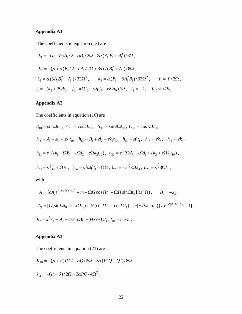
where the coefficients 1l , 2l , ik and 1f are defined in Appendix A1. Here, it has been
assumed that the steady state response starts at time instant 0t from the initial condition
sxtx −=)( 0 and remains thereafter in the normal operating region sxtx ≤|)(| until
moment 1t . Since the origin of the starting time has been set by a choice of the forcing
term in equations (13), it is not possible to set 00 =t . It is easy to see from equation (13)
that three secular terms do not have enough time to grow and lead to an unbounded
response in the steady state response, because both the time interval )/,0()( 01 Ω∈− π tt
and time ] ,[ 10 ttt∈ for undergoing this motion are finite and small. Thus, the nominal
secular terms in the solution expressions need not be eliminated properly as is necessary
when the usual perturbation method is applicable for seeking an approximate solution for
a uniformly weakly nonlinear equation [1-5].
For the second segment of the motion, the solution to the linear equation (6b) can be
expressed in the form:
10
tHtGttmBeAty ttc Ω+Ω+−++= −− cossin)()( 12)(
21 , for syty ≥|)(| , (14)
where 2A , 2B and 1t are constants to be determined, cyFm sat /)sgn(−= ,
)(/ 22 Ω+Ω= ccfG , )/( 22 Ω+−= cfH .
At this point it is clear that there are six unknowns associated with the problem; that is,
four constants 1A , 1B , 2A , 2B , and two crossing times 0t and 1t . These constants can be
determined by implementing an appropriate set of initial conditions as well as periodicity,
continuity and symmetry conditions, which can be expressed as follows:
sxtx −=)( 0 , sxtx =)( 1 , sxty 21
)( 1 ε= , )()( 1121
txty && ε=
sxty 21
)( 2 ε= , )()( 0221
txty && ε−= , 02 tt +Ω
=π . (15a-g)
Here, the last two conditions arise from the symmetry of the solution being examined.
The four unknown constants iA , iB , ( 2,1 =i ) can be determined as functions of the
system parameters and two crossing times 0t and 1t by imposing conditions (15a, c, e, f).
Then substituting these constants into the corresponding solutions and imposing
conditions (15b, d) yields a set of two transcendental equations for unknown 0t and 1t as
follows:
sxChShthChSh =++Ω++ 3016301511310121011 sin ,
23026302512412310221021 cossin cAmChShththChSh −=++Ω+Ω++ , (16)
where the coefficients 10S , 10C , 30S , 30C , and ijh are given in Appendix A2.
Equation (16) involves system parameters and two unknown crossing times 0t and 1t
only. It is evident that no analytical solutions to equation (16) can be found, and thus
numerical means have to be adopted to solve the crossing times for all possible solutions.
11
The constants iA , iB , ( 2,1 =i ) can be evaluated after obtaining an appropriate value for
the time instants 0t and 1t . Then the corresponding histories of )(tx and )(ty can be
calculated from equations (8) and (14). This procedure completes the determination of
the symmetric periodic solution with a doubly-entering saturation region per cycle.
4. Stability of the periodic solutions
Due to the non-smooth nonlinearities of magnetic force occurring at the boundaries of
the saturation region, the stability of the periodic solution can only be determined by
investigating the asymptotic behavior of perturbations to the steady-state periodic
solution, as the usual method involving the classical Floquet theory is not applicable to
such a non-smooth system.
Let )(tX and )(tz denote the corresponding perturbed solutions to )(tx and )(ty ,
respectively. Performing a similar procedure as used in determining the approximate
solution, the first-order approximate perturbed solution of the first segment under the
perturbed initial conditions, sxttX −=∆+ )( 00 , 0000 )( vvttX ∆+=∆+& , can be written as:
)()()( 10 tXtXtX ε+= , for sxtX ≤|)(| , (17)
with
ττ Ω+Ω= cossin)( 110 QPtX , (18)
+Ω+Ω= ττ cossin)( 211 LLtX ττ Ωsin1K + ττ Ωcos2K ttf Ω+ sin1
ττ Ω+Ω+ 3cos3sin 43 KK , (19)
where 00 ttt ∆−−=τ , 0v represents the initial velocity of the response at time 0t , and the
operator,∆ , denotes a small perturbation of the operand. Since the perturbations in the
initial conditions are assumed to be small, it is expected that the coefficients in equations
12
(18) and (19) will assume values close to those of the unperturbed motions, respectively
[23]. To the first order, the coefficients in equation (18) are given by:
Ω∆+= /01 vPP , QQ =1 , (20)
where Ω= /0vP , sxQ −= , are determined by applying the unperturbed initial conditions
sxtX −=)( 0 , 00 )( vtX =& , in the corresponding unperturbed solution. The coefficients in
equation (19) can be expressed as:
02010 tlvlLL iiii ∆+∆+= , ,2,1 =i
010 vkKK jjj ∆+= , , 4,3,2,1=j (21)
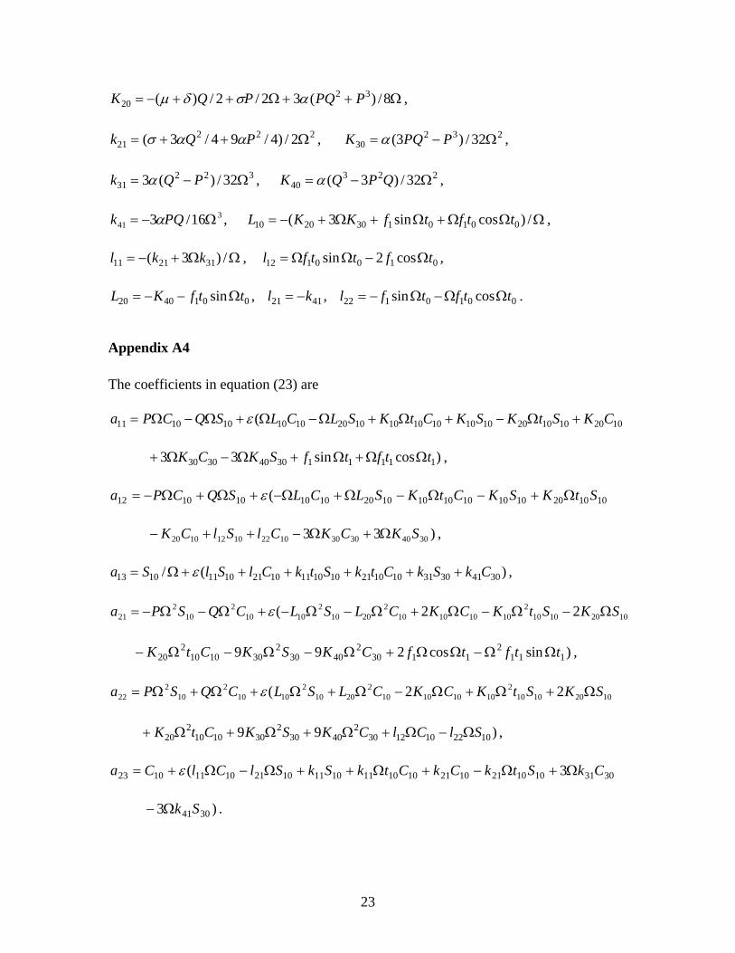
where the coefficients 0iL , 1il , 2il , 0jK , and 1jk are defined in Appendix A3.
At the time instant, 11 ttt ∆+= , the motion of the first segment reaches the upper
boundary of the saturation region and will enter the saturation zone thereafter. The
perturbed response at the moment of entrance is assumed to be:
sxttX =∆+ )( 11 , 1111 )( vvttX ∆+=∆+& , (22)
where 1v represents the velocity of the unperturbed response of the first segment at 1t .
Substituting equation (17) into equation (22) and keeping only the first-order terms yields
0013012111 =∆+∆+∆ vatata ,
0230221211 vatatav ∆+∆+∆=∆ , (23)
where the coefficients ija are given in Appendix A4.
The asymptotic behaviour of the perturbed motion for the second segment of the
response from time )( 11 tt ∆+ to )( 22 tt ∆+ can be investigated using the same procedure
13
performed as that for the first segment. Similarly, the solution under the perturbed initial
conditions, sxttz 21
)( 11 ε=∆+ , )()( 111121
vvttz ∆+=∆+ ε& , can be written in the form:
tHtGtttmQePtz tttc Ω+Ω+∆−−++= ∆−−− cossin)()( 112)(
211 , (24)
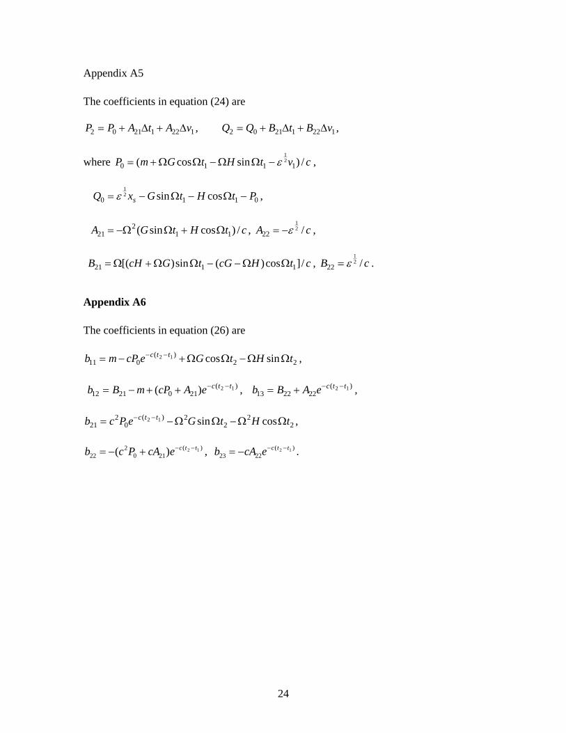
where the coefficients 2P and 2Q are given in Appendix A5.
The perturbed response at the time instant )( 22 tt ∆+ is assumed to be:
sxttz 21
)( 22 ε=∆+ , )()( 222221
vvttz ∆+=∆+ ε& , (25)
where 221
vε denotes the velocity of the unperturbed response of the second segment at 2t .
Substituting equation (24) into (25), performing some algebraic manipulations and
retaining terms up to the first order, yields the following equations:
0113112211 =∆+∆+∆ vbtbtb ,
21
/)( 1231222212 εvbtbtbv ∆+∆+∆=∆ , (26)
where the coefficients ijb are defined in Appendix A6.
Equations (23) and (26) can be expressed in matrix form as:
⎥⎦
⎤⎢⎣
⎡∆∆
=⎥⎦
⎤⎢⎣
⎡∆∆
0
0
1
1
vt
Rvt
, ⎥⎦
⎤⎢⎣
⎡∆∆
=⎥⎦
⎤⎢⎣
⎡∆∆
1
1
2
2
vt
Uvt
, (27)
where R is a 22× matrix with elements, 111211 / aar −= , 111312 / aar −= ,
1112212221 / aaaar −= , 1113212322 / aaaar −= , respectively, and U is a 22× matrix with
elements, 111211 / bbu −= , 111312 / bbu −= , 21
/)/( 1112212221 εbbbbu −= ,
21
/)/( 1113212322 εbbbbu −= , respectively.
The small perturbations of the symmetric solution during the first half period of the
motion are obtained by combining the two equations given by (27) to form an equation
14
⎥⎦
⎤⎢⎣
⎡∆∆
=⎥⎦
⎤⎢⎣
⎡∆∆
0
0
2
2
vt
Jvt
, (28)
where J represents the transition matrix for the response from time instant )( 00 tt ∆+ to
)( 22 tt ∆+ , and is given by RUJ = . The stability of the steady-state solution is
determined by the eigenvalues of this transition matrix. Denoting the trace of J by TJ
and the determinant of J by DJ , the two eigenvalues of the matrix are given by:
])4([ 212
21
2,1 DJTJTJ −±=λ . (29)
The symmetric period-one motion is asymptotically stable if both eigenvalues 1λ and 2λ
of matrix J have a modulus less than unity. When either of the two eigenvalues has a
modulus greater than one, the solution is unstable. From the proceeding discussion, it
may be deduced that all elements of matrix J are functions of the system parameters and
the crossing times, which cannot be given explicitly. This means that it is not possible to
obtain explicit expressions in terms of the system parameters for the trace and
determinant of matrix J. Nevertheless, by substituting the expressions for the elements of
matrices R and U and performing some algebraic manipulations, the determinants of
matrices R and U, namely DR and DU, may be eventually expressed in a simple form as:
)()()]()(1[
1
0210 tx
txOtDR&
&εδµε ++−= ,
)()(
2
1)( 12
tytyeDU ttc
&
&−−= . (30)
By imposing continuity and periodicity conditions of the symmetric solution, i.e.,
)()( 1121
txty && ε= , )()( 0221
txty && ε−= , the determinant of matrix J, as the product of the traces
of matrices R and U, is of a quite simple form:
)]()(1[ 210
)( 12 εδµε OteDJ ttc ++−−= −− . (31)
15
Based on the fact that the dimensionless damping coefficient c (i.e. εµ ) and the
dimensionless derivative gain d (i.e. εδ ) are positive and much smaller than unity for a
practical example, and that 1|)()(1| 210 <++− εδµε Ot always holds, it can be
concluded from equation (31) that 1|| <DJ . This indicates that no Hopf bifurcation is
possible in the symmetric motion examined for a practical system. As the system
parameters are changed, the modulus of one eigenvalue may take the value of unity,
where a bifurcation occurs. One possible way for an eigenvalue to cross the unit circle is
through +1, which corresponds to a saddle-node, pitchfork or transcritical bifurcation.
The other way is through –1, which relates to a period-doubling bifurcation. The stability
boundaries 1±=λ can be established by solving the equation:
01 =+TJDJ m . (32)
It may be noted that equation (32) involves trigonometric and exponential function terms
which depend on the crossing times 1t and 0t . This implies that the stability diagrams
cannot be built up analytically. In addition, since the determination of 1t and 0t depends
on the roots of the two transendental equations given by (16), a numerical construction of
the stability diagrams will be an extremely laborious task. Thus the construction of
stability diagrams is not pursued in the present work.
5. Comparison of the approximate and exact solutions
To validate the present analytical results, the symmetric periodic solutions determined
by the developed analysis were compared with the exact solutions. The classical fourth-
order Runge-Kutta algorithm was employed to perform the numerical integration of
equation (6). It was found that the approximate solutions obtained by the developed
16
analysis and the exact numerical solutions are in an excellent agreement for the case of
primary resonances.
An approximate solution and its stability can be easily constructed and examined
using the methodology developed in Sections 3 and 4. For example, in the case 1.0=c ,
3.0=d , 4.1=p , 4.0=F , 65.0=Ω , and 0.1=ε , the analysis in Section 3 gives that
397921.00 =t , 683299.11 =t . The coefficients in equations (12), (13) and (14) can be
easily obtained by a back substitution. Then the solution expressions can be easily written
out. Two eigenvalues of the transition matrix J for the solution are calculated to be
48002.01 =λ , 72654.02 −=λ , which indicates the approximate solution is stable. Figure
3 shows the phase portraits of the analytical approximate solution and exact solution
obtained from numerical integration. The solid curve indicates the results of numerical
integration and the circles represent the approximate solution. The differences between
the approximate and exact solutions are very small. The approximate solution is in good
agreement with the exact solution. The dashed curve in Figure 3 represents the results of
numerical integration of the corresponding linear equation when the non-linearity terms
in equation (6a) are neglected. It is noted that the solution of the corresponding linear
system is not able to be a representation to the solution of the nonlinear system.
Figure 4 shows the maximum amplitudes of the dynamic response of two systems with
the variation of the dimensionless proportional gain p in the region ]21.2,81.1[ ∈p ,
which corresponds to the external detuning in the region ]21.0,19.0[ −∈σ . The system
parameters for System I are 05.0=d , 05.0=c , 25.0=F , 0.1=Ω , 0.1=ε , and those
for System II are 2.0=d , 2.0=c , 45.0=F , 0.1=Ω , 0.1=ε , respectively. The circles
in Figure 4 indicate values of the amplitudes obtained by the developed analysis and
17
triangles indicate the numerical simulation values. The discrepancies between the first-
order approximate analytical solutions and exact numerical solutions are between
%036.0− and %047.0− for System I, and between %504.0 and %741.0 for System II.
Figure 5 shows the maximum amplitude of the response of Systems III and IV with
the variation of the dimensionless forcing frequency in the region ]15.2 ,85.1[∈Ω , which
corresponds to the external detuning in the region ]6225.0 ,5775.0[−∈σ . The system
parameters for System III are 05.0=c , 05.0=d , 0.5=p , 9.0=F , 0.1=ε , and those
for System IV are 2.0=c , 6.0=d , 0.5=p , 25.1=F , 0.1=ε . The discrepancies
between the approximate and exact solutions for System III are between %023.0 and
%053.0 , and between %468.0 and %578.0 for System IV. The differences between the
approximate and exact solutions for small values of the system parameters are hardly
distinguishable by the naked eye (as shown in Figures 4(a) and 5(a)). For large values of
the system parameters, the approximate solutions give slightly smaller values of the
maximum response amplitude than those of the exact solutions (as shown in Figures 4(b)
and 5(b)). The first order approximate solutions match well with the numerical exact
solutions.
It can be concluded from Figures (4) and (5) that only small differences between the
first-order approximate and exact solutions are found. The first order approximate
solutions can give excellent representations of the exact solutions. Additional higher-
order terms may be included in the approximate solution if a solution of higher accuracy
is required, but it seems unnecessary.
18
6. Conclusion
An approximate periodic solution of a piecewise nonlinear-linear oscillator has been
analytically determined using a new methodology, as no exact solution exists in closed-
form. The mathematical model of the oscillator is characterized by a combination of a
weakly nonlinear and a linear differential equation. More specially, the response of the
weakly nonlinear system is studied for the case of primary resonances, which may lead to
secular terms in the steady sate response of a uniformly weakly nonlinear system. The
methodology developed here involved combining an asymptotic expansion solution to the
weakly nonlinear system and an exact solution to the linear system. By imposing an
appropriate set of matching and periodicity conditions, the task of determining a periodic
symmetric solution with a doubly-entering saturation zone per cycle was eventually
reduced to a set of two transcendental algebraic equations. The stability characteristic of
the symmetric solution was based on examining the propagation of small perturbations in
the initial conditions over a half period of the response. The accuracy of the first-order
approximate solutions was confirmed by comparison with the results obtained by direct
integration of the original equations of motion. More importantly, the methodology
developed can be applied to other types of non-smooth systems, which are characterized
by different forms of equations of motion.
Acknowledgements
This work was supported by the Australian Research Council under the Discovery-
Project Grant DP0343396. The authors would like to thank three anonymous referees
for their valuable comments and suggestions.
19
References
1. A. H. Nayfeh, D. T. Mook, Nonlinear Oscillations, John Wiley & Sons, New
York, 1979.
2. P. Hagedorn, Non-linear Oscillations, Second Edition, Clarendon Press, Oxford,
1988.
3. J. J. Stoker, Nonlinear Vibrations in Mechanical and Electrical Systems, John
Wiley & Sons, New York, 1992.
4. R. E. Mickens, Oscillations in Planar Dynamic Systems, World Scientific
Publishing Co. Pte. Ltd., Singapore, 1996.
5. J. M. T. Thompson, H. B. Stewart, Nonlinear Dynamics and Chaos, John Wiley
and Sons, Chichester, 1998 .
6. Y. B. Kim, S. K. Choi, A multiple harmonic balance method for the internal
resonant vibration of a non-linear Jeffcott rotor, Journal of Sound and Vibration
208 (1997) 745-761.
7. C. J. Begley and L. N. Virgin, Impact response and the influence of friction,
Journal of Sound and Vibration 211 (1998) 801-818..
8. Y. Kang, S. S. Shyr, Y. F. Chang, S. C. Jen, Frequency-locked motion and quasi-
periodic motion of s piecewise-linear system subjected to externally nonlinear
synchronous excitations, Journal of Sound and Vibration 214 (1998) 377-382.
9. A. Maccari, The response of a forced oscillator under the effect of a pair of set-up
elastic stops, Journal of Sound and Vibration 235 (2000) 879-887.
20
10. S. Natsiavas, S. Theodossiades, and I. Goudas, Dynamic analysis of piecewise
linear oscillators with time periodic coefficients, International Journal of Non-
Linear Mechanics 35 (2000) 53-68.
11. M. Wiercigroch, Mathematical models of mechanical systems with
discontinuities, in Applied Nonlinear Dynamics and Chaos of Mechanical Systems
with Discontinuities (M. Wiercigroch and B. de Kraker, editors), World
Scientific, Singapore, 2000, pp.17-36
12. B. de Kraker, J. A. W. van der Spek and D. H. van Campen, Extensions of cell
mapping for discontinuous systems, in Applied Nonlinear Dynamics and Chaos of
Mechanical Systems with Discontinuities (M. Wiercigroch and B. de Kraker,
editors), World Scientific, Singapore, 2000, pp.61-102.
13. S. Natsiavas, Dynamics of piecewise linear oscillators, in Applied Nonlinear
Dynamics and Chaos of Mechanical Systems with Discontinuities (M.
Wiercigroch and B. de Kraker, editors), World Scientific, Singapore, 2000,
pp.127-159.
14. J. Warminski, G. Litak and K. Szabelski, Dynamic phenomena in gear boxes, in
Applied Nonlinear Dynamics and Chaos of Mechanical Systems with
Discontinuities (M. Wiercigroch and B. de Kraker editors), World Scientific,
Singapore, 2000, pp.177-205.
15. E. Chicurel-Uziel, Exact, single equation, closed-form solution of vibrating
systems with piecewise linear springs, Journal of Sound and Vibration 245 (2001)
285-301
21
16. E. V. Karpenko, M. Wiercigroch, E. E. Pavlovskaia, M. P. Cartmell, Piecewise
approximate analytical solutions for a Jeffcott rotr with a snubber ring,
International Journal of Mechanical Sciences 44 (2002) 475-488.
17. S. Lei, A. Palazzolo and A. F. Kascak, Fuzzy logic control of magnetic bearings
for suspension of vibration due to sudden imbalance, Proceedings of the Fifth
International Symposium on Magnetic Suspension Technology, California, 1999,
pp.459-471.
18. N. M. Thibeault, R. Smith, B. Paden and J. Antaki, Achievable robustness
comparison of position sensed and self-sensing magnetic bearing systems,
Proceedings of the Fifth International Symposium on Magnetic Suspension
Technology, California, 1999, pp.563-573.
19. G. Schweitzer, H. Bleuler and A. Traxler, Active Magnetic Bearings, Basics,
Properties and Application of Active Magnetic Bearings, Switzerland: Verlag der
Fachwereine (vdf), ETH-Zurich, 1994.
20. A. H. Nayfeh, Perturbation Methods, John Wiley & Sons, New York, 1973.
21. E. J. Hinch, Perturbation Methods, Cambridge University Press, Cambridge,
1991.
22. C. F. Chan Man Fong, D. De Chee, Perturbation Methods, Instability,
Catastrophe, and Chaos, World Scientific, Singapore, 1999.
23. M. P. Karyeaclis and T. K. Caughey, Stability of a semi-active impact damper:
part II, periodic solutions, American Society of Mechanical Engineers Journal of
Applied Mechanics 56 (1989) 930-940.
22
Appendix A1
The coefficients in equation (13) are
Ω+−Ω−+−= 8/)(32/2/)( 311
21111 ABABAk ασδµ ,
Ω++Ω++−= 8/)(32/2/)( 31
211112 ABAABk ασδµ ,
231
2113 32/)3( Ω−= ABAk α , 2
121
314 32/)3( Ω−= BABk α , Ω= 2/1 ff ,
ΩΩΩ+Ω+Ω+−= /)cossin3( 00101321 ttftfkkl , 00142 sin ttfkl Ω−−= .
Appendix A2
The coefficients in equation (16) are
1010 sin tS Ω= , 1010 cos tC Ω= , 1030 3sin tS Ω= , 1030 3cos tC Ω= ,
1011111 tklAh εε ++= , 1022112 tklBh εε ++= , 1113 tfh ε= , 315 kh ε= , 416 kh ε= ,
)( 1022112121
tklBkh Ω−Ω−Ω−= εεεε , )( 1012112221
tkklAh Ω++Ω+Ω= εεεε ,
Hfh Ω+= 12323
ε , Gtfh Ω−Ω= 112423
ε , 425 323
kh Ω−= ε , 326 323
kh Ω= ε ,
with
)/(]sincos[ 21
1000
)/(21 ΩΩΩ−ΩΩ+−= −Ω− επ tHtGmecAA tc , sxB −=1 ,
)]/()cos(cos)sin(sin[ 1010102 tmttHttGA −Ω−Ω+Ω+Ω+Ω= π ]1/[ )/( 10 −−Ω− tce π ,
1122 cossin21
tHtGAxB s Ω−Ω−−= ε , 0110 ttt −= .
Appendix A3
The coefficients in equation (21) are
Ω+−Ω−+−= 8/)(32/2/)( 3210 QQPQPK ασδµ ,
211 4/32/)( Ω−Ω+−= PQk αδµ ,
23
Ω++Ω++−= 8/)(32/2/)( 3220 PPQPQK ασδµ ,
22221 2/)4/94/3( Ω++= PQk αασ , 232
30 32/)3( Ω−= PPQK α ,
32231 32/)(3 Ω−= PQk α , 223
40 32/)3( Ω−= QPQK α ,
341 16/3 Ω−= PQk α , ΩΩΩ+Ω+Ω+−= /)cossin3( 00101302010 ttftfKKL ,
ΩΩ+−= /)3( 312111 kkl , 0100112 cos2sin tfttfl Ω−ΩΩ= ,
0014020 sin ttfKL Ω−−= , 4121 kl −= , 0010122 cossin ttftfl ΩΩ−Ω−= .
Appendix A4
The coefficients in equation (23) are
1020101020101010101010201010101011 ( CKStKSKCtKSLCLSQCPa +Ω−+Ω+Ω−Ω+Ω−Ω= ε
)cossin33 1111130403030 ttftfSKCK ΩΩ+Ω+Ω−Ω+ ,
101020101010101010201010101012 ( StKSKCtKSLCLSQCPa Ω+−Ω−Ω+Ω−+Ω+Ω−= ε
)33 30403030102210121020 SKCKClSlCK Ω+Ω−++− ,
)(/ 30413031101021101011102110111013 CkSkCtkStkClSlSa ++++++Ω= ε ,
102010102
101010102
20102
10102
102
21 22( SKStKCKCLSLCQSPa Ω−Ω−Ω+Ω−Ω−+Ω−Ω−= ε
)sincos299 1112
11302
40302
3010102
20 ttftfCKSKCtK ΩΩ−ΩΩ+Ω−Ω−Ω− ,
102010102
101010102
20102
10102
102
22 22( SKStKCKCLSLCQSPa Ω+Ω+Ω−Ω+Ω+Ω+Ω= ε
)99 10221012302
40302
3010102
20 SlClCKSKCtK Ω−Ω+Ω+Ω+Ω+ ,
303110102110211010111011102110111023 3( CkStkCkCtkSkSlClCa Ω+Ω−+Ω++Ω−Ω+= ε
)3 3041SkΩ− .
24
Appendix A5
The coefficients in equation (24) are
12212102 vAtAPP ∆+∆+= , 12212102 vBtBQQ ∆+∆+= ,
where cvtHtGmP /)sincos( 111021
ε−ΩΩ−ΩΩ+= ,
0110 cossin21
PtHtGxQ s −Ω−Ω−= ε ,
ctHtGA /)cossin( 112
21 Ω+ΩΩ−= , cA /21
22 ε−= ,
ctHcGtGcHB /]cos)(sin)[( 1121 ΩΩ−−ΩΩ+Ω= , cB /21
22 ε= .
Appendix A6
The coefficients in equation (26) are
22)(
011 sincos12 tHtGecPmb ttc ΩΩ−ΩΩ+−= −− ,
)(2102112
12)( ttceAcPmBb −−++−= , )(222213
12 ttceABb −−+= ,
22
22)(
02
21 cossin12 tHtGePcb ttc ΩΩ−ΩΩ−= −− ,
)(210
222
12)( ttcecAPcb −−+−= , )(2223
12 ttcecAb −−−= .
25
A list of legends for the figures
Figure 1. A single-degree-of-freedom magnetic bearing.
Figure 2. A symmetric period-one motion with a doubly-entering saturation zone per
cycle; )(tx denotes the segment of motion in the normal operating region
sxtx ≤|)(| , )(ty represents the segment in the saturation region syty ≥|)(| ,
0t denotes the starting time, and it .)4,3,2,1( =i the time instants that the
non-smooth nonlilnearities take place, sy± indicate the boundaries of
saturation zone.
Figure 3. The phase portraits of the approximate and exact solution; solid curve
indicates the direct numerical integration results, circles represent the
analytical approximate solution, dashed curve denotes the numerical results
of integration of the corresponding linear equations.
Figure 4. The variation of the maximum amplitudes of the response of the overall
system given by equation (6) with the proportional gain p; Circles denote the
approximate solutions and triangles represent results of the numerical
integration; (a) System I, (b) System II.
Figure 5. The variation of the maximum amplitudes of the response of the overall
system given by equation (6) with the forcing frequency Ω ; Circles denote
the approximate solutions and triangles represent results of the numerical
integration; (a) System III, (b) System IV.


