Embed Size (px)
Citation preview
IEEE TRANSACTIONS ON AUTOMATIC CONTROL, VOL. 48, NO. 12, DECEMBER 2003 2089
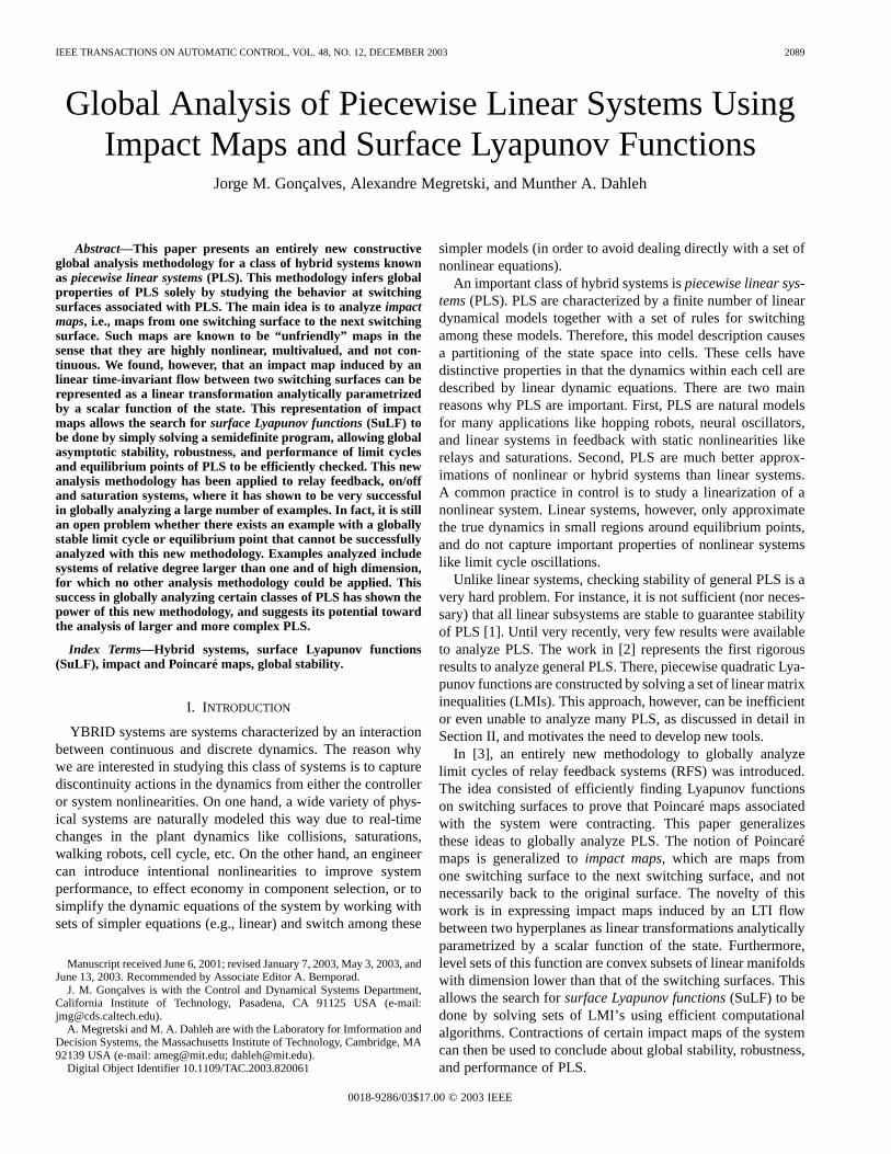
Global Analysis of Piecewise Linear Systems UsingImpact Maps and Surface Lyapunov Functions
Jorge M. Gonçalves, Alexandre Megretski, and Munther A. Dahleh
Abstract—This paper presents an entirely new constructiveglobal analysis methodology for a class of hybrid systems knownas piecewise linear systems(PLS). This methodology infers globalproperties of PLS solely by studying the behavior at switchingsurfaces associated with PLS. The main idea is to analyzeimpactmaps, i.e., maps from one switching surface to the next switchingsurface. Such maps are known to be “unfriendly” maps in thesense that they are highly nonlinear, multivalued, and not con-tinuous. We found, however, that an impact map induced by anlinear time-invariant flow between two switching surfaces can berepresented as a linear transformation analytically parametrizedby a scalar function of the state. This representation of impactmaps allows the search forsurface Lyapunov functions(SuLF) tobe done by simply solving a semidefinite program, allowing globalasymptotic stability, robustness, and performance of limit cyclesand equilibrium points of PLS to be efficiently checked. This newanalysis methodology has been applied to relay feedback, on/offand saturation systems, where it has shown to be very successfulin globally analyzing a large number of examples. In fact, it is stillan open problem whether there exists an example with a globallystable limit cycle or equilibrium point that cannot be successfullyanalyzed with this new methodology. Examples analyzed includesystems of relative degree larger than one and of high dimension,for which no other analysis methodology could be applied. Thissuccess in globally analyzing certain classes of PLS has shown thepower of this new methodology, and suggests its potential towardthe analysis of larger and more complex PLS.
Index Terms—Hybrid systems, surface Lyapunov functions(SuLF), impact and Poincaré maps, global stability.
I. INTRODUCTION
YBRID systems are systems characterized by an interactionbetween continuous and discrete dynamics. The reason whywe are interested in studying this class of systems is to capturediscontinuity actions in the dynamics from either the controlleror system nonlinearities. On one hand, a wide variety of phys-ical systems are naturally modeled this way due to real-timechanges in the plant dynamics like collisions, saturations,walking robots, cell cycle, etc. On the other hand, an engineercan introduce intentional nonlinearities to improve systemperformance, to effect economy in component selection, or tosimplify the dynamic equations of the system by working withsets of simpler equations (e.g., linear) and switch among these
Manuscript received June 6, 2001; revised January 7, 2003, May 3, 2003, andJune 13, 2003. Recommended by Associate Editor A. Bemporad.
J. M. Gonçalves is with the Control and Dynamical Systems Department,California Institute of Technology, Pasadena, CA 91125 USA (e-mail:[email protected]).
A. Megretski and M. A. Dahleh are with the Laboratory for Imformation andDecision Systems, the Massachusetts Institute of Technology, Cambridge, MA92139 USA (e-mail: [email protected]; [email protected]).
Digital Object Identifier 10.1109/TAC.2003.820061
simpler models (in order to avoid dealing directly with a set ofnonlinear equations).
An important class of hybrid systems ispiecewise linear sys-tems(PLS). PLS are characterized by a finite number of lineardynamical models together with a set of rules for switchingamong these models. Therefore, this model description causesa partitioning of the state space into cells. These cells havedistinctive properties in that the dynamics within each cell aredescribed by linear dynamic equations. There are two mainreasons why PLS are important. First, PLS are natural modelsfor many applications like hopping robots, neural oscillators,and linear systems in feedback with static nonlinearities likerelays and saturations. Second, PLS are much better approx-imations of nonlinear or hybrid systems than linear systems.A common practice in control is to study a linearization of anonlinear system. Linear systems, however, only approximatethe true dynamics in small regions around equilibrium points,and do not capture important properties of nonlinear systemslike limit cycle oscillations.
Unlike linear systems, checking stability of general PLS is avery hard problem. For instance, it is not sufficient (nor neces-sary) that all linear subsystems are stable to guarantee stabilityof PLS [1]. Until very recently, very few results were availableto analyze PLS. The work in [2] represents the first rigorousresults to analyze general PLS. There, piecewise quadratic Lya-punov functions are constructed by solving a set of linear matrixinequalities (LMIs). This approach, however, can be inefficientor even unable to analyze many PLS, as discussed in detail inSection II, and motivates the need to develop new tools.
In [3], an entirely new methodology to globally analyzelimit cycles of relay feedback systems (RFS) was introduced.The idea consisted of efficiently finding Lyapunov functionson switching surfaces to prove that Poincaré maps associatedwith the system were contracting. This paper generalizesthese ideas to globally analyze PLS. The notion of Poincarémaps is generalized toimpact maps, which are maps fromone switching surface to the next switching surface, and notnecessarily back to the original surface. The novelty of thiswork is in expressing impact maps induced by an LTI flowbetween two hyperplanes as linear transformations analyticallyparametrized by a scalar function of the state. Furthermore,level sets of this function are convex subsets of linear manifoldswith dimension lower than that of the switching surfaces. Thisallows the search forsurface Lyapunov functions(SuLF) to bedone by solving sets of LMI’s using efficient computationalalgorithms. Contractions of certain impact maps of the systemcan then be used to conclude about global stability, robustness,and performance of PLS.
0018-9286/03$17.00 © 2003 IEEE
2090 IEEE TRANSACTIONS ON AUTOMATIC CONTROL, VOL. 48, NO. 12, DECEMBER 2003
We will show that this new methodology can be used tonot only globally analyze limit cycles but also equilibriumpoints of PLS. For that, on/off and saturation systems areanalyzed, including those with unstable nonlinearity sectorsfor which classical methods like Popov criterion, Zames–Falbcriterion [4], integral quadratic constraints (IQCs) [5]–[8], failto analyze. In addition, the results in [9] and [10, Ch. 8]show that this methodology can also be efficiently applied toanalyze robustness and performance of PLS. Thus, the successin globally analyzing stability, robustness, and performanceof certain classes of PLS has shown the power of this newmethodology, and suggests its potential toward the analysisof larger and more complex PLS.
This paper is organized as follows. The next section moti-vates the need for new analysis tools for PLS by explaining howavailable methods can be inefficient or even unable to analyzemany PLS. Sections III and IV are dedicated to the developmentthe main tool that relaxes the problem of checking contractionof impact maps to solving a semidefinite program. Then, Sec-tion V explains how this is used to globally analyze PLS. Theseresults are applied to globally analyze asymptotic stability ofon/off and saturation systems, in Sections VI and VII, respec-tively. Section VIII shows how less conservative global stabilityconditions can be obtained. Conclusions and future work arediscussed in Section IX and, finally, technical details are con-sidered in the Appendix.
II. M OTIVATION
As discussed in introduction, there exist several tools toanalyze PLS. One of the most important consists of con-structing piecewise quadratic Lyapunov functions (PQLFs)in the state–space [2], [11], [12]. This method relaxes theproblem to a solution of a finite-dimensional set of LMIs.There are, however, several drawbacks with this approach thatmotivates the need for alternative methods to analyze PLS.These drawbacks are as follows.
• PQLF cannot analyze limit cycles since PQLF constructsLyapunov functions in the state space.
• For most PLS, it is not possible to construct PQLF withjust the given natural partition of the system. In order toimprove flexibility, a refinement of partitions is typicallynecessary. The analysis method, however, is efficient onlywhen the number of partitions required to prove stabilityis small. Example 2.1 below shows that even for secondorder systems, the construction of PQLF can be computa-tionally intractable due to the large number of partitionsin the state–space required for the analysis.
• In general, for systems of order higher than 3, it isextremely hard to obtain a refinement of partitions inthe state-space to efficiently analyze PLS using PQLF.In other words, the method does not scale well with thedimension of the system. In fact, only a few and specificexamples of PLS of order higher than 3 analyzed withthis method have been reported.
• Existence of PQLF implies exponential stability of thesystem. Thus, PQLF cannot prove asymptotic stability ofPLS that are not exponentially stable.
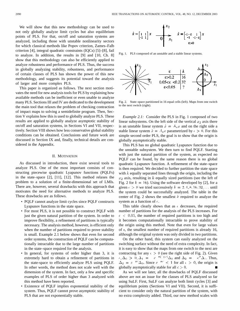
Fig. 1. PLS composed of an unstable and a stable linear systems.
Fig. 2. State–space partitioned in 16 equal cells (left). Maps from one switchto the next switch (right).
Example 2.1:Consider the PLS in Fig. 1 composed of twolinear subsystems. On the left side of the verticalaxis thereis an unstable linear system and on the right side astable linear system parametrized by . For thissimple second order PLS, the goal is to show that the origin isglobally asymptotically stable.
This PLS has no global quadratic Lyapunov function due tothe unstable subsystem. We then turn to find PQLF. Startingwith just the natural partition of the system, as expected noPQLF can be found, by the same reason there is no globalquadratic Lyapunov function. A refinement of the state–spaceis then required. We decided to further partition the state spacewith equally separated lines through the origin, including the
axis, resulting in equally sized partitions (see the left ofFig. 2 for ). Using the software developed by [2], for agiven we tried successively untilthe system could be successfully analyzed. The table in thecenter of Fig. 2 shows the smallestrequired to analyze thesystem as a function of.
This table clearly shows that asdecreases, the requirednumber of partitions for the analysis of the PLS increases. For
, the number of required partitions is too high andit becomes computationally intractable to prove stability ofthe origin using this method. Note that even for large valuesof , the smallest number of required partitions is already 16,although the original system was only divided in two partitions.
On the other hand, this system can easily analyzed on theswitching surface without the need of extra complexity. In fact,it is easy to show that the maps from one switch to the next arecontracting for any (see the right side of Fig. 2). Given
and . Thus,. Since for all , the origin is
globally asymptotically stable for all .As we will see later, all the drawbacks of PQLF discussed
above are not an issue for the classes of PLS analyzed so farusing SuLF. First, SuLF can analyze both limit cycles [3] andequilibrium points (Sections VI and VII). Second, it is suffi-cient to consider only the natural partition of the system, withno extra complexity added. Third, our new method scales with
GONÇALVESet al.: GLOBAL ANALYSIS OF PIECEWISE LINEAR SYSTEMS 2091
the dimension of the system, and, finally, SuLF can be used toprove global asymptotic stability of PLS that are not exponen-tially stable (see example 7.3).
Also, the construction of PQLF for PLS proposed in [2] im-poses continuity of the the Lyapunov functions along switchingsurfaces. This means that the intersection of two quadraticLyapunov functions with a switching surface—one from eachside—defines a unique quadratic Lyapunov function on theswitching surface. Therefore, existence of PQLF guaranteethe existence of SuLF. The converse, however, is not true. Forinstance, SuLF exist to analyze limit cycles [3], but no PQLFexist in the state–space.
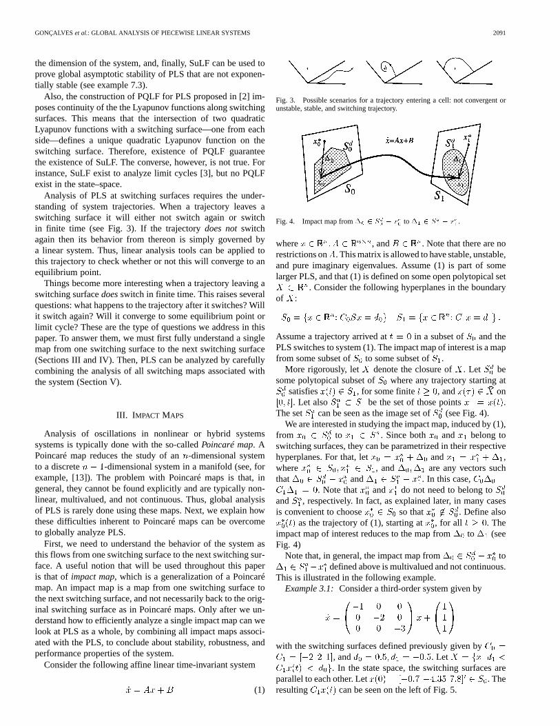
Analysis of PLS at switching surfaces requires the under-standing of system trajectories. When a trajectory leaves aswitching surface it will either not switch again or switchin finite time (see Fig. 3). If the trajectorydoes notswitchagain then its behavior from thereon is simply governed bya linear system. Thus, linear analysis tools can be applied tothis trajectory to check whether or not this will converge to anequilibrium point.
Things become more interesting when a trajectory leaving aswitching surfacedoesswitch in finite time. This raises severalquestions: what happens to the trajectory after it switches? Willit switch again? Will it converge to some equilibrium point orlimit cycle? These are the type of questions we address in thispaper. To answer them, we must first fully understand a singlemap from one switching surface to the next switching surface(Sections III and IV). Then, PLS can be analyzed by carefullycombining the analysis of all switching maps associated withthe system (Section V).
III. I MPACT MAPS
Analysis of oscillations in nonlinear or hybrid systemssystems is typically done with the so-calledPoincaré map. APoincaré map reduces the study of an-dimensional systemto a discrete -dimensional system in a manifold (see, forexample, [13]). The problem with Poincaré maps is that, ingeneral, they cannot be found explicitly and are typically non-linear, multivalued, and not continuous. Thus, global analysisof PLS is rarely done using these maps. Next, we explain howthese difficulties inherent to Poincaré maps can be overcometo globally analyze PLS.
First, we need to understand the behavior of the system asthis flows from one switching surface to the next switching sur-face. A useful notion that will be used throughout this paperis that of impact map, which is a generalization of a Poincarémap. An impact map is a map from one switching surface tothe next switching surface, and not necessarily back to the orig-inal switching surface as in Poincaré maps. Only after we un-derstand how to efficiently analyze a single impact map can welook at PLS as a whole, by combining all impact maps associ-ated with the PLS, to conclude about stability, robustness, andperformance properties of the system.
Consider the following affine linear time-invariant system
(1)
Fig. 3. Possible scenarios for a trajectory entering a cell: not convergent orunstable, stable, and switching trajectory.
Fig. 4. Impact map from� 2 S � x to� 2 S � x .
where , and . Note that there are norestrictions on . This matrix is allowed to have stable, unstable,and pure imaginary eigenvalues. Assume (1) is part of somelarger PLS, and that (1) is defined on some open polytopical set
. Consider the following hyperplanes in the boundaryof :
Assume a trajectory arrived at in a subset of and thePLS switches to system (1). The impact map of interest is a mapfrom some subset of to some subset of .
More rigorously, let denote the closure of . Let besome polytopical subset of where any trajectory starting at
satisfies , for some finite , and on. Let also be the set of those points .
The set can be seen as the image set of(see Fig. 4).We are interested in studying the impact map, induced by (1),
from to . Since both and belong toswitching surfaces, they can be parametrized in their respectivehyperplanes. For that, let and ,where , and are any vectors suchthat and . In this case,
. Note that and do not need to belong toand , respectively. In fact, as explained later, in many casesis convenient to choose so that . Define also
as the trajectory of (1), starting at , for all . Theimpact map of interest reduces to the map fromto (seeFig. 4)
Note that, in general, the impact map from todefined above is multivalued and not continuous.
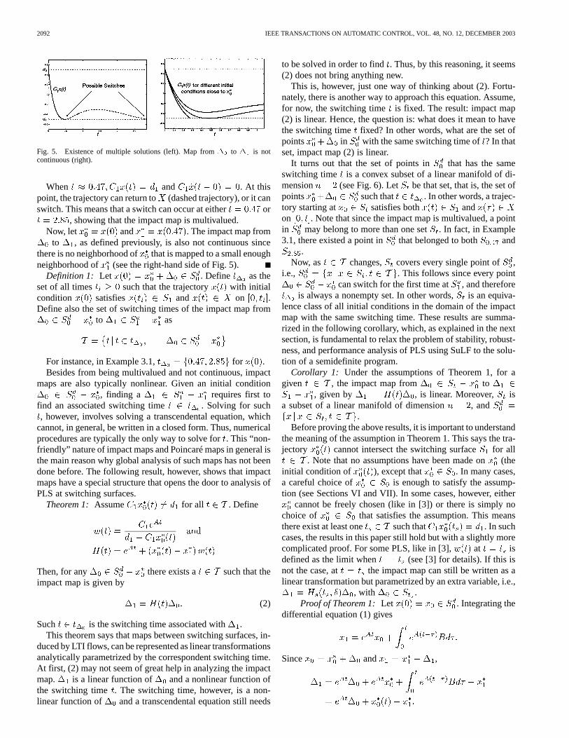
This is illustrated in the following example.Example 3.1:Consider a third-order system given by
with the switching surfaces defined previously given by, and . Let. In the state space, the switching surfaces are
parallel to each other. Let . Theresulting can be seen on the left of Fig. 5.
2092 IEEE TRANSACTIONS ON AUTOMATIC CONTROL, VOL. 48, NO. 12, DECEMBER 2003
Fig. 5. Existence of multiple solutions (left). Map from� to � is notcontinuous (right).
When and . At thispoint, the trajectory can return to (dashed trajectory), or it canswitch. This means that a switch can occur at either or
, showing that the impact map is multivalued.Now, let and . The impact map from
to , as defined previously, is also not continuous sincethere is no neighborhood of that is mapped to a small enoughneighborhood of (see the right-hand side of Fig. 5).
Definition 1: Let . Define as theset of all times such that the trajectory with initialcondition satisfies and on .Define also the set of switching times of the impact map from
to as
For instance, in Example 3.1, for .Besides from being multivalued and not continuous, impact
maps are also typically nonlinear. Given an initial condition, finding a requires first to
find an associated switching time . Solving for such, however, involves solving a transcendental equation, which
cannot, in general, be written in a closed form. Thus, numericalprocedures are typically the only way to solve for. This “non-friendly” nature of impact maps and Poincaré maps in general isthe main reason why global analysis of such maps has not beendone before. The following result, however, shows that impactmaps have a special structure that opens the door to analysis ofPLS at switching surfaces.
Theorem 1: Assume for all . Define
Then, for any there exists a such that theimpact map is given by
(2)
Such is the switching time associated with .This theorem says that maps between switching surfaces, in-
duced by LTI flows, can be represented as linear transformationsanalytically parametrized by the correspondent switching time.At first, (2) may not seem of great help in analyzing the impactmap. is a linear function of and a nonlinear function ofthe switching time . The switching time, however, is a non-linear function of and a transcendental equation still needs
to be solved in order to find. Thus, by this reasoning, it seems(2) does not bring anything new.
This is, however, just one way of thinking about (2). Fortu-nately, there is another way to approach this equation. Assume,for now, the switching time is fixed. The result: impact map(2) is linear. Hence, the question is: what does it mean to havethe switching time fixed? In other words, what are the set ofpoints in with the same switching time of? In thatset, impact map (2) is linear.
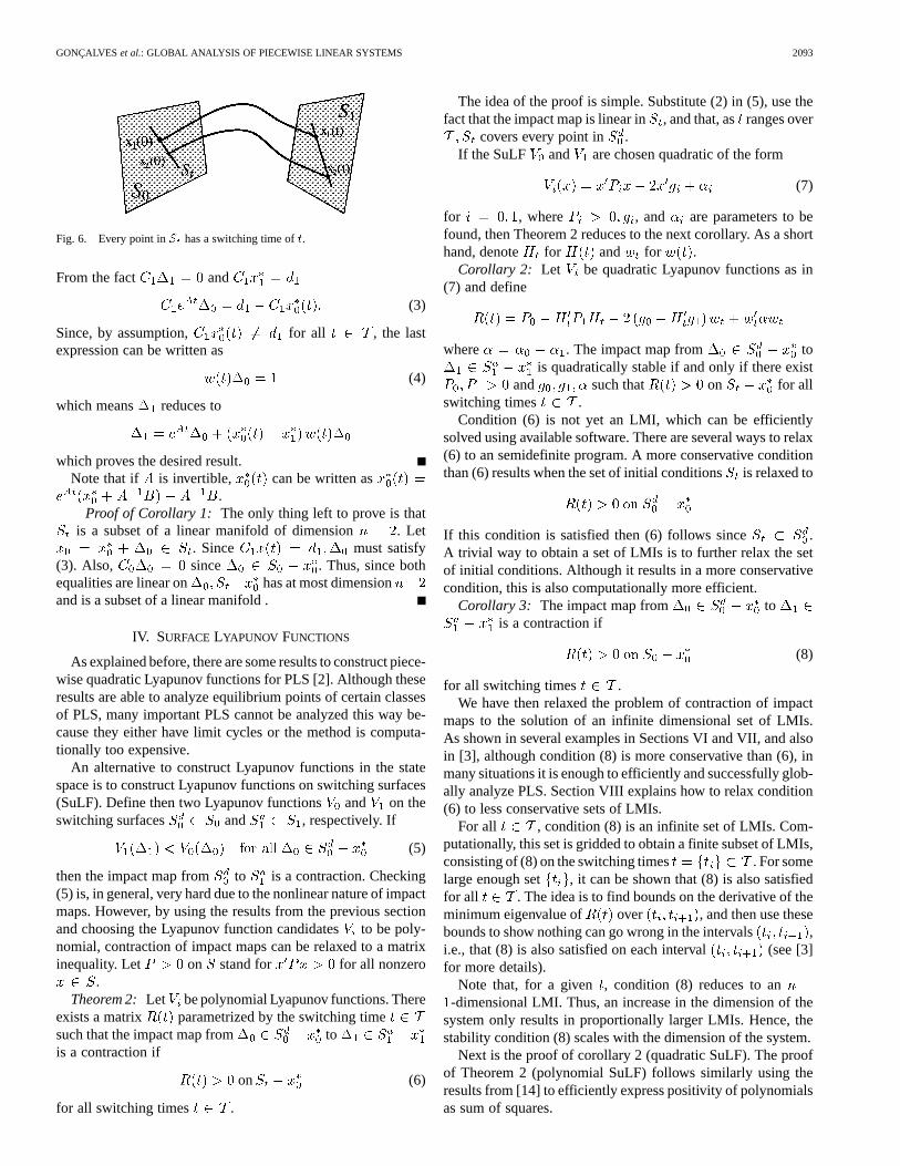
It turns out that the set of points in that has the sameswitching time is a convex subset of a linear manifold of di-mension (see Fig. 6). Let be that set, that is, the set ofpoints such that . In other words, a trajec-tory starting at satisfies both andon . Note that since the impact map is multivalued, a pointin may belong to more than one set. In fact, in Example3.1, there existed a point in that belonged to both and
.Now, as changes, covers every single point of ,
i.e., . This follows since every pointcan switch for the first time at , and therefore
is always a nonempty set. In other words,is an equiva-lence class of all initial conditions in the domain of the impactmap with the same switching time. These results are summa-rized in the following corollary, which, as explained in the nextsection, is fundamental to relax the problem of stability, robust-ness, and performance analysis of PLS using SuLF to the solu-tion of a semidefinite program.
Corollary 1: Under the assumptions of Theorem 1, for agiven , the impact map from to
, given by , is linear. Moreover, isa subset of a linear manifold of dimension , and
.Before proving the above results, it is important to understand
the meaning of the assumption in Theorem 1. This says the tra-jectory cannot intersect the switching surface for all
. Note that no assumptions have been made on(theinitial condition of ), except that . In many cases,a careful choice of is enough to satisfy the assump-tion (see Sections VI and VII). In some cases, however, either
cannot be freely chosen (like in [3]) or there is simply nochoice of that satisfies the assumption. This meansthere exist at least one such that . In suchcases, the results in this paper still hold but with a slightly morecomplicated proof. For some PLS, like in [3], at isdefined as the limit when (see [3] for details). If this isnot the case, at the impact map can still be written as alinear transformation but parametrized by an extra variable, i.e.,
, with .Proof of Theorem 1:Let . Integrating the
differential equation (1) gives
Since and ,
GONÇALVESet al.: GLOBAL ANALYSIS OF PIECEWISE LINEAR SYSTEMS 2093
Fig. 6. Every point inS has a switching time oft.
From the fact and
(3)
Since, by assumption, for all , the lastexpression can be written as
(4)
which means reduces to
which proves the desired result.Note that if is invertible, can be written as
.Proof of Corollary 1: The only thing left to prove is that
is a subset of a linear manifold of dimension . Let. Since must satisfy
(3). Also, since . Thus, since bothequalities are linear on has at most dimensionand is a subset of a linear manifold .
IV. SURFACE LYAPUNOV FUNCTIONS
As explained before, there are some results to construct piece-wise quadratic Lyapunov functions for PLS [2]. Although theseresults are able to analyze equilibrium points of certain classesof PLS, many important PLS cannot be analyzed this way be-cause they either have limit cycles or the method is computa-tionally too expensive.
An alternative to construct Lyapunov functions in the statespace is to construct Lyapunov functions on switching surfaces(SuLF). Define then two Lyapunov functions and on theswitching surfaces and , respectively. If
(5)
then the impact map from to is a contraction. Checking(5) is, in general, very hard due to the nonlinear nature of impactmaps. However, by using the results from the previous sectionand choosing the Lyapunov function candidatesto be poly-nomial, contraction of impact maps can be relaxed to a matrixinequality. Let on stand for for all nonzero
.Theorem 2: Let be polynomial Lyapunov functions. There
exists a matrix parametrized by the switching timesuch that the impact map from tois a contraction if
on (6)
for all switching times .
The idea of the proof is simple. Substitute (2) in (5), use thefact that the impact map is linear in, and that, asranges over
covers every point in .If the SuLF and are chosen quadratic of the form
(7)
for , where , and are parameters to befound, then Theorem 2 reduces to the next corollary. As a shorthand, denote for and for .
Corollary 2: Let be quadratic Lyapunov functions as in(7) and define
where . The impact map from tois quadratically stable if and only if there exist
and such that on for allswitching times .
Condition (6) is not yet an LMI, which can be efficientlysolved using available software. There are several ways to relax(6) to an semidefinite program. A more conservative conditionthan (6) results when the set of initial conditionsis relaxed to
If this condition is satisfied then (6) follows since .A trivial way to obtain a set of LMIs is to further relax the setof initial conditions. Although it results in a more conservativecondition, this is also computationally more efficient.
Corollary 3: The impact map from tois a contraction if
(8)
for all switching times .We have then relaxed the problem of contraction of impact
maps to the solution of an infinite dimensional set of LMIs.As shown in several examples in Sections VI and VII, and alsoin [3], although condition (8) is more conservative than (6), inmany situations it is enough to efficiently and successfully glob-ally analyze PLS. Section VIII explains how to relax condition(6) to less conservative sets of LMIs.
For all , condition (8) is an infinite set of LMIs. Com-putationally, this set is gridded to obtain a finite subset of LMIs,consisting of (8) on the switching times . For somelarge enough set , it can be shown that (8) is also satisfiedfor all . The idea is to find bounds on the derivative of theminimum eigenvalue of over , and then use thesebounds to show nothing can go wrong in the intervals ,i.e., that (8) is also satisfied on each interval (see [3]for more details).
Note that, for a given , condition (8) reduces to an-dimensional LMI. Thus, an increase in the dimension of the
system only results in proportionally larger LMIs. Hence, thestability condition (8) scales with the dimension of the system.
Next is the proof of corollary 2 (quadratic SuLF). The proofof Theorem 2 (polynomial SuLF) follows similarly using theresults from [14] to efficiently express positivity of polynomialsas sum of squares.
2094 IEEE TRANSACTIONS ON AUTOMATIC CONTROL, VOL. 48, NO. 12, DECEMBER 2003
Proof of Corollary 2: From (5) and (7), and using The-orem 1
Finally, using (4), we have
Condition (6) follows from corollary 1.
V. GLOBAL ANALYSIS OF PLS
In the previous section, we showed how a single impact mapcan be efficiently globally analyzed using SuLF. This sectionbriefly explains how impact maps associated with PLS are com-bined to globally analyze the system (details are left to Sec-tions VI and VII). There are basically three main steps to achievethis goal: characterization of impact maps, definition of SuLF,and solution of stability conditions.
Step 1) Impact Maps
a) Identification of all impact maps associatedwith the PLS. If the system has switchingsurfaces then there are at most impactmaps. The actual number of impact mapsrequired to analyze the system is typicallysmaller due to certain properties of a systemlike symmetries or just the fact that not allswitches are possible.
b) In order to reduce conservatism, it is importantto characterize the domain of each impactmap, as explained in Section VIII.A. Impactmaps that have an empty domain do not needto be further considered, neither those pointsin switching surfaces that converge asymp-totically to an equilibrium point withoutswitching (see the middle of Fig. 3). Also,certain necessary conditions must be checkedto guarantee that a trajectory, starting in aswitching surface, does not grow unboundedwithout switching (as in the left of Fig. 3).
c) For each impact map find the set of switchingtimes .
d) For each impact map, find an belonging tothe hyperplane where the domain of an im-pact is defined, such that the assumption ofTheorem 1 is satisfied. If this is not possible,characterize the switching times where the as-sumption is not satisfied and then proceed asexplained in Section III.
Step 2) SuLF
a) Define all SuLF on the respective domains ofimpact maps.
b) Characterize constraints on SuLF related withcontinuity across boundaries, and with equi-librium points or limit cycles that belong to orintersect the domain of impact maps.
Step 3) Stability Conditions
a) For each impact map, Theorem 2 provides sta-bility conditions (6) that can be relaxed toLMIs like (8). The stability conditions mustthen be solved simultaneously to find the pa-rameters of the SuLF.
b) Bounds on switching times. For many impactmaps, it is sufficient to check the associatedstability condition (6) on a bounded subset ofswitching times , instead of all .
c) Improvement of stability conditions. If theLMIs provided by Corollary 3 fail to finda feasible solution then less conservativeconditions can be used, as explained in Sec-tion VIII.
d) An alternative to solve the above set of LMIs isto consecutively add new LMI’s until the sta-bility conditions are satisfied, since checkingan LMI is much easier than solving it. The fol-lowing algorithm can be used instead.
i) Initialize the SuLF with some parame-ters. The set of LMIs is an empty set atthis time.
ii) Check if the stability conditions aresatisfied for all switching times (orswitching times bounds).
iii) If not, take a switching time where itwas not satisfied and add a new LMIto the set of LMIs. Solve this new setof LMIs, get new parameters for theSuLF, and go back to ii). If yes, thealgorithm ends.
To better understand each of the above steps in analyzing PLSwith SuLF, several classes of PLS are considered. Each of theseclasses was carefully chosen to separately deal with differentissues in each step of the algorithm, and to illustrate with exam-ples the efficiency of this new methodology. By increasing com-plexity, we first analyzed limit cycles of relay feedback systems(RFS) [3]. For symmetric unimodal limit cycles there is onlya single impact map that needs to be studied. This means thatglobal analysis of symmetric unimodal limit cycles of RFS fol-lows directly from Theorem 2.
Then, Section VI analyzes on/off systems to explain howthis new methodology is used to globally analyze equilibriumpoints, and how more than one impact map is simultaneouslyanalyzed. Finally, Section VII considers saturation systems toshow how to deal with multiple switching surfaces. The suc-cess in globally analyzing a large number of examples of theseclasses of PLS demonstrated the potential of these new resultsin globally analyzing other, more complex classes of PLS usinga combination of the ideas discussed above.
VI. ON–OFF SYSTEMS (OFS)
This section addresses the problem of global stability anal-ysis of OFS. An OFS can be thought of as an LTI system thatswitches between closed (on) and open (off) loop, or as a lower
GONÇALVESet al.: GLOBAL ANALYSIS OF PIECEWISE LINEAR SYSTEMS 2095
bound saturation. OFS can be found in many biological and en-gineering applications. In biology, concentrations of substrateshave a lower bound saturation since they must always be posi-tive. In electronic circuits, diodes can be approximated by on/offnonlinearities. Also, transient behavior of logical circuits thatinvolve latches/flip-flops performing on/off switching can bemodeled with on/off circuits and saturations. In aircraft control[1], a max controller was designed to achieve good tracking ofthe pilot’s input without violating safety margins.
As in RFS, a large number of examples is successfullyproven globally stable, including systems with unstable sub-systems, systems of relative degree larger than one and of highdimension, and systems with unstable nonlinearity sectors,for which classical methods like small gain theorem, Popovcriterion, Zames–Falb criterion [4], and integral quadraticconstraints [5]–[8], fail to analyze. In fact, it is still an openproblem whether there exists an example with a globally stableequilibrium point that could not be successfully analyzed withthis new methodology.
A. Problem Formulation
This section starts by defining OFS and giving some neces-sary conditions for the global stability of a unique locally stableequilibrium point. Consider a SISO LTI system
(9)
where , in feedback with an on/off controller (see Fig. 7)given by
(10)
where . By a solution of (9) and (10), we mean func-tions satisfying (9) and (10). Sinceis continuous andglobally Lipschitz, is also globally Lipschitz. Thus,the OFS has a unique solution for any initial state.
In the state–space, the on/off controller introduces aswitching surface composed of an hyperplane of dimension
given by
On one side of the switching surface , the system isgiven by . On the other side , the system isgiven by , where
and . The vector field is continuous alongthe switching surface since for any .
OFS have either zero, one, two, or a continuum of nonisolatedequilibrium points. To be globally stable, an OFS needs to havea unique locally stable equilibrium point. Next are necessaryconditions for the existence of a single locally stable equilibriumpoint for different values of .
If there is at least one equilibrium point at the origin. Inthis case, it is necessary thatis Hurwitz to guarantee the originis locally stable. If is invertible, the subsystemhas an equilibrium point at . To guarantee the OFShas only one equilibrium point at the origin, it is necessary that
. It is also necessary that has no real unstable
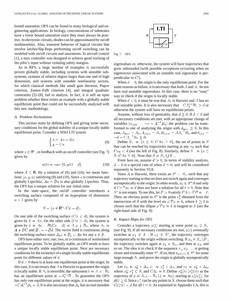
Fig. 7. OFS.
eigenvalues or, otherwise, the system will have trajectories thatgrow unbounded (with possible exceptions occurring when aneigenvector associated with an unstable real eigenvalue is per-pendicular to ).
When , the origin is the only equilibrium point. For thesame reasons as before, it is necessary that bothand do nothave real unstable eigenvalues. In this case, there is no “easy”way to check if the origin is locally stable.
When , it must be true that is Hurwitz and has noreal unstable poles. It is also necessary that orotherwise the system will have no equilibrium points.
Assume, without loss of generality, that . If andall necessary conditions are met, with an appropriate change ofvariables the problem can be trans-formed to one of analyzing the origin with . In thiscase, , and
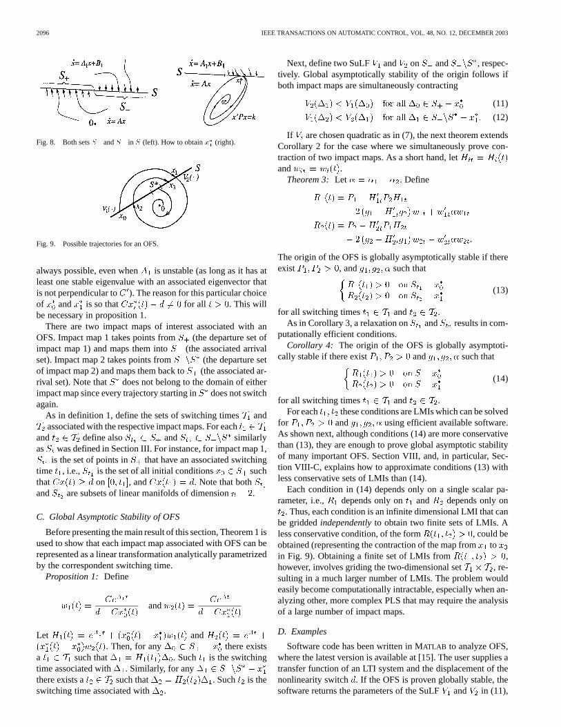
.Define , the set of points in
that can be reached by trajectories starting at anysuch that(see the left of Fig. 8). Similarly, define
. Note that .From here on, assume . In terms of stability analysis,
is a special case of when , and will be consideredseparately in Section VI.E.
Since is Hurwitz, there exists an such that anytrajectory starting in that set does not switch again and convergesasymptotically to the origin. In other words, if and onlyif does not have a solution for all . Note that
is not empty. To see this, let satisfy .Then, an obvious point in is the point obtained from theintersection of with the level set , where ischosen such that the ellipse is tangent to (see theright-hand side of Fig. 8).
B. Impact Maps for OFS
Consider a trajectory starting at some point(see Fig. 9). If all necessary conditions are met, eventuallyswitches at . If , the trajectory convergesasymptotically to the origin without switching. If ,the trajectory switches again at , and then at , andso on. The idea is to check if the sequence is gettingcloser and eventually enter . If so, then for somelarge enough , and prove the origin is globally asymptoticallystable.
Let , and ,where , and . Define as thetrajectory of , starting at , forall . Since can be any points in, choose them such that
for all . As explained in Appendix I.A, this is
2096 IEEE TRANSACTIONS ON AUTOMATIC CONTROL, VOL. 48, NO. 12, DECEMBER 2003
Fig. 8. Both setsS andS in S (left). How to obtainx (right).
Fig. 9. Possible trajectories for an OFS.
always possible, even when is unstable (as long as it has atleast one stable eigenvalue with an associated eigenvector thatis not perpendicular to ). The reason for this particular choiceof and is so that for all . This willbe necessary in proposition 1.
There are two impact maps of interest associated with anOFS. Impact map 1 takes points from (the departure set ofimpact map 1) and maps them into (the associated arrivalset). Impact map 2 takes points from (the departure setof impact map 2) and maps them back to (the associated ar-rival set). Note that does not belong to the domain of eitherimpact map since every trajectory starting indoes not switchagain.
As in definition 1, define the sets of switching times andassociated with the respective impact maps. For each
and define also and similarlyas was defined in Section III. For instance, for impact map 1,
is the set of points in that have an associated switchingtime , i.e., is the set of all initial conditions suchthat on , and . Note that bothand are subsets of linear manifolds of dimension .
C. Global Asymptotic Stability of OFS
Before presenting the main result of this section, Theorem 1 isused to show that each impact map associated with OFS can berepresented as a linear transformation analytically parametrizedby the correspondent switching time.
Proposition 1: Define
and
Let and. Then, for any there exists
a such that . Such is the switchingtime associated with . Similarly, for anythere exists a such that . Such is theswitching time associated with .
Next, define two SuLF and on and , respec-tively. Global asymptotically stability of the origin follows ifboth impact maps are simultaneously contracting
(11)
(12)
If are chosen quadratic as in (7), the next theorem extendsCorollary 2 for the case where we simultaneously prove con-traction of two impact maps. As a short hand, letand .
Theorem 3: Let . Define
The origin of the OFS is globally asymptotically stable if thereexist , and such that
(13)
for all switching times and .As in Corollary 3, a relaxation on and results in com-
putationally efficient conditions.Corollary 4: The origin of the OFS is globally asymptoti-
cally stable if there exist and such that
(14)
for all switching times and .For each these conditions are LMIs which can be solved
for and using efficient available software.As shown next, although conditions (14) are more conservativethan (13), they are enough to prove global asymptotic stabilityof many important OFS. Section VIII, and, in particular, Sec-tion VIII-C, explains how to approximate conditions (13) withless conservative sets of LMIs than (14).
Each condition in (14) depends only on a single scalar pa-rameter, i.e., depends only on and depends only on
. Thus, each condition is an infinite dimensional LMI that canbe griddedindependentlyto obtain two finite sets of LMIs. Aless conservative condition, of the form , could beobtained (representing the contraction of the map fromtoin Fig. 9). Obtaining a finite set of LMIs from ,however, involves griding the two-dimensional set , re-sulting in a much larger number of LMIs. The problem wouldeasily become computationally intractable, especially when an-alyzing other, more complex PLS that may require the analysisof a large number of impact maps.
D. Examples
Software code has been written in MATLAB to analyze OFS,where the latest version is available at [15]. The user supplies atransfer function of an LTI system and the displacement of thenonlinearity switch . If the OFS is proven globally stable, thesoftware returns the parameters of the SuLFand in (11),
GONÇALVESet al.: GLOBAL ANALYSIS OF PIECEWISE LINEAR SYSTEMS 2097
(12). The MATLAB function also plots the minimum eigenvaluesof each in (14) on a finite subset of . Bounds on max-imum switching times are considered in Appendix I.C. Also,certain necessary conditions imposed at are discussed inAppendix I-B.
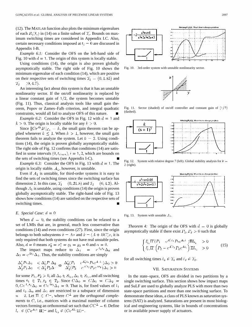
Example 6.1:Consider the OFS on the left-hand side ofFig. 10 with . The origin of this system is locally stable.
Using conditions (14), the origin is also proven globallyasymptotically stable. The right side of Fig. 10 shows theminimum eigenvalue of each condition (14), which are positiveon their respective sets of switching times and
.An interesting fact about this system is that it has an unstable
nonlinearity sector. If the on/off nonlinearity is replaced bya linear constant gain of , the system becomes unstable(Fig. 11). Thus, classical analysis tools like small gain the-orem, Popov or Zames–Falb criterion, and integral quadraticconstraints, would all fail to analyze OFS of this nature.
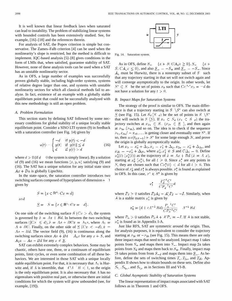
Example 6.2:Consider the OFS in Fig. 12 with and. The origin is locally stable for any .
Since , the small gain theorem can be ap-plied whenever . When , however, the small gaintheorem fails to analyze the system. Let . Using condi-tions (14), the origin is proven globally asymptotically stable.The right side of Fig. 12 confirms that conditions (14) are satis-fied in some intervals , which are bounds onthe sets of switching times (see Appendix I-C).
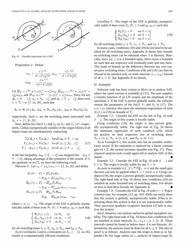
Example 6.3:Consider the OFS in Fig. 13 with . Theorigin is locally stable. , however, is unstable.
Even if is unstable, for third-order systems it is easy tofind the sets of switching times since the switching surface hasdimension 2. In this case, and . Al-though is unstable, using conditions (14) the origin is provenglobally asymptotically stable. The right-hand side of Fig. 13shows how conditions (14) are satisfied on the respective sets ofswitching times.
E. Special Case:
When , the stability conditions can be relaxed to aset of LMIs that are, in general, much less conservative thanconditions (14) and even conditions (27). First, since the originbelongs to both subsystems and , it isonly required that both systems do not have real unstable poles.Also, means and .
The impact maps reduce to and. Thus, the stability conditions are simply
for some , all , and all switchingtimes . Since
. That is, for fixed values ofand and are restricted to a subspace of dimension
. Let , where are theorthogonal comple-mentsto , i.e., matrices with a maximal number of columnvectors forming an orthonormal set such that . Define
and .
Fig. 10. 3rd-order system with unstable nonlinearity sector.
Fig. 11. Sector (shaded) of on/off controller and constant gain of(1=2)(dashed).
Fig. 12. System with relative degree 7 (left). Global stability analysis fork =2 (right).
Fig. 13. System with unstableA .
Theorem 4: The origin of the OFS with is globallyasymptotically stable if there exist such that
(15)
for all switching times and .
VII. SATURATION SYSTEMS
In the state–space, OFS are divided in two partitions by asingle switching surface. This section shows how impact mapsand SuLF are used to globally analyze PLS with more than twostate-space partitions and more than one switching surface. Todemonstrate these ideas, a class of PLS known assaturation sys-tems(SAT) is analyzed. Saturations are present in most biolog-ical and engineering systems, like in bounds of concentrationsor in available power supply of actuators.
2098 IEEE TRANSACTIONS ON AUTOMATIC CONTROL, VOL. 48, NO. 12, DECEMBER 2003
It is well known that linear feedback laws when saturatedcan lead to instability. The problem of stabilizing linear systemswith bounded controls has been extensively studied. See, forexample, [16]–[18] and the references therein.
For analysis of SAT, the Popov criterion is simple but con-servative. The Zames–Falb criterion [4] can be used when thenonlinearity’s slope is restricted, but the method is difficult toimplement. IQC-based analysis [5]–[8] gives conditions in theform of LMIs that, when satisfied, guarantee stability of SAT.However, none of these analysis tools can be used when a SAThas an unstable nonlinearity sector.
As in OFS, a large number of examples was successfullyproven globally stable, including high-order systems, systemsof relative degree larger than one, and systems with unstablenonlinearity sectors for which all classical methods fail to an-alyze. In fact, existence of an example with a globally stableequilibrium point that could not be successfully analyzed withthis new methodology is still an open problem.
A. Problem Formulation
This section starts by defining SAT followed by some nec-essary conditions for global stability of a unique locally stableequilibrium point. Consider a SISO LTI system (9) in feedbackwith a saturation controller (see Fig. 14) given by
(16)
where (if the system is simply linear). By a solutionof (9) and (16) we mean functions satisfying (9) and(16). The SAT has a unique solution for any initial state since
is globally Lipschitz.In the state–space, the saturation controller introduces two
switching surfaces composed of hyperplanes of dimensiongiven by
On one side of the switching surface , the systemis governed by . In between the two switchingsurfaces , where
. Finally, on the other side of. The vector field (9), (16) is continuous along the
switching surfaces since for any , andfor any .
SAT can exhibit extremely complex behaviors. Some may bechaotic, others have one, three, or a continuum of equilibriumpoints, limit cycles, or even some combination of all these be-haviors. We are interested in those SAT with a unique locallystable equilibrium point. For that, it is necessary thatis Hur-witz and, if is invertible, that , so the originis the only equilibrium point. It is also necessary thathas noeigenvalues with positive real part, or otherwise there are initialconditions for which the system will grow unbounded (see, forexample, [19]).
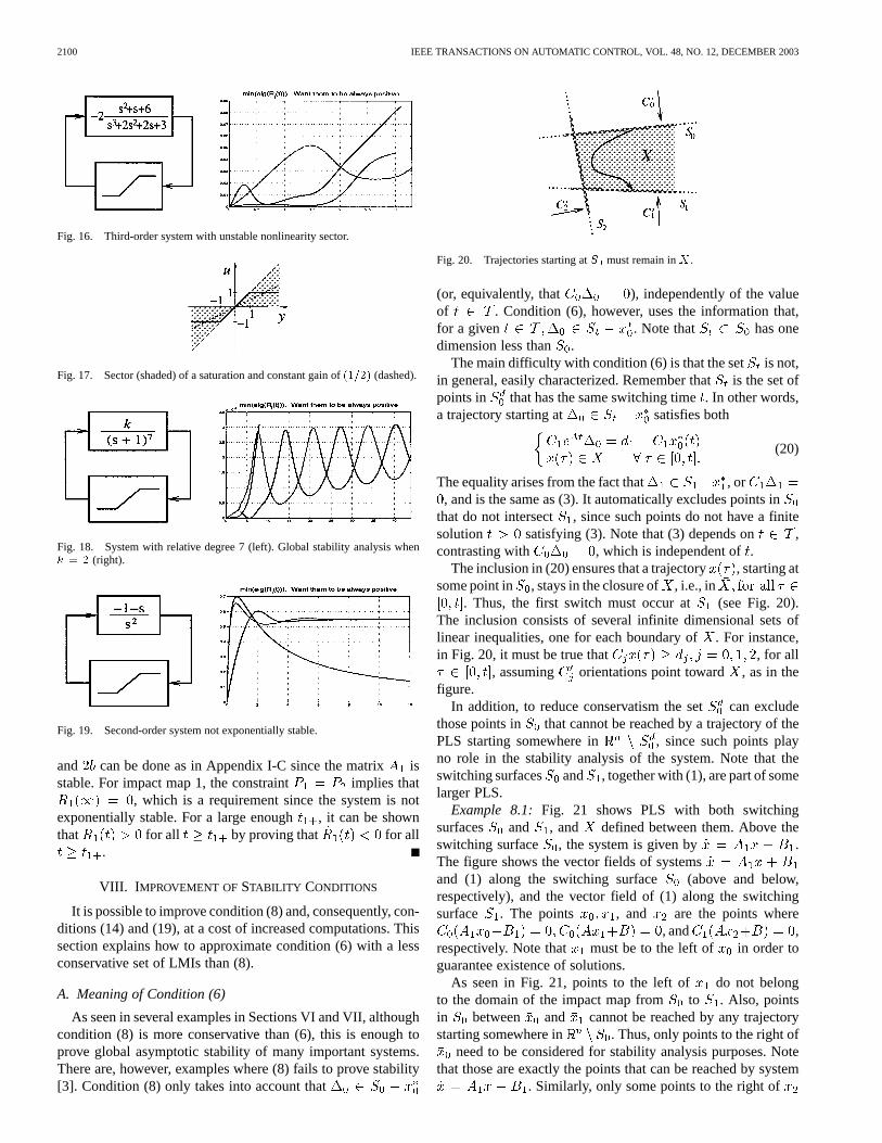
Fig. 14. Saturation system.
As in OFS, define, and also and . Since
must be Hurwitz, there is a nonempty subset of suchthat any trajectory starting in that set will not switch again andwill converge asymptotically to the origin. In other words, let
be the set of points such that donot have a solution for any .
B. Impact Maps for Saturation Systems
The strategy of the proof is similar to OFS. The main differ-ence is that a trajectory starting in can also switch at
(see Fig. 15). Let be the set of points inthat will switch in . If the tra-jectory switches at , and then againat , and so on. The idea is to check if the sequence
is getting closer and eventually enter. Ifso, then for some large enough , and provethe origin is globally asymptotically stable.
Let , , and, where and . Define
as the trajectory of ,starting at , for all . Since are any points in
, they are chosen such that for all . Thischoice of and is always possible. is found as explainedin OFS. In this case, is given by
where satisfies . Similarly, whenis a stable matrix is given by
where satisfies . If is not stable,is found as in Appendix I-A.
Just like RFS, SAT are symmetric around the origin. Thus,for analysis purposes, it is equivalent to consider the trajectorystarting at or (see Fig. 15). This means there are onlythree impact maps that need to be analyzed. Impact map 1 takespoints from and maps them into . Impact map takespoints from and maps them back to . Finally, impact map
takes points from from and maps them into . As be-fore, define the sets of switching times , and . Ap-pendix II shows how to obtain bounds on these sets. Define also
, and as in Sections III and VI-B.
C. Global Asymptotic Stability of Saturation Systems
The linear representation of impact maps associated with SATfollows as in Theorem 1 and OFS.
GONÇALVESet al.: GLOBAL ANALYSIS OF PIECEWISE LINEAR SYSTEMS 2099
Fig. 15. Possible trajectories for a SAT.
Proposition 2: Define
Let, and . Then, for any
, , and , there exist, such that
respectively. Such are the switching times associated with.
Next, define two SuLF and on and , respec-tively. Global asymptotically stability of the origin follows if allimpact maps are simultaneously contracting
(17)
In the last inequality, was mapped into, taking advantage of the symmetry of the system. If
are quadratic as in (7), we have the following result.Theorem 5: Let and define
where . The origin of the SAT is globally asymp-totically stable if there exist and such that
(18)
for all switching times , and .As in Corollaries 3 and 4, a relaxation on
results in computationally efficient conditions.
Corollary 5: The origin of the SAT is globally asymptoti-cally stable if there exist and such that
(19)
for all switching times , and .In many cases, conditions (18) and (19) do not need to be sat-
isfied for all switching times. Appendix II shows how boundson switching times can be obtained whenis Hurwitz. Basi-cally, since is a bounded input, there exists a boundedset such that any trajectory will eventually enter and stay there.This leads to bounds on the difference between any two con-secutive switching times. Conditions (18) and (19) can then berelaxed to be satisfied only on some intervals insteadof all . See Appendix II for details.
D. Examples
Software code has been written in MATLAB to analyze SAT,where the latest version is available at [15]. The user suppliesa transfer function of an LTI system and the amplitude of thesaturation . If the SAT is proven globally stable, the softwarereturns the parameters of the SuLF and in (17). Thematlab function also plots the minimum eigenvalues of each
in (19) on bounds of .Example 7.1:Consider the SAT on the left of Fig. 16 with
. The origin of this system is locally stable.Using conditions (19), the origin is also proven glob-
ally asymptotically stable. The right side of Fig. 16 showsthe minimum eigenvalue of each condition (19), whichare positive on their respective sets of switching times
, and .As in Example 6.1, this system also has an unstable nonlin-
earity sector. If the saturation is replaced by a linear constantgain of , the system becomes unstable (see Fig. 17). Thus,classical analysis tools would again fail to analyze SAT of thisnature.
Example 7.2:Consider the SAT in Fig. 18 with and. The origin is locally stable for any .
As seen in example 6.2, and the small gaintheorem can only be applied when . Let . Using con-ditions (19), the origin is proven globally asymptotically stable.The right-hand side of Fig. 18 shows how conditions (19) aresatisfied on some bounded sets of switching times. For detailson how to find these bounds see Appendix II.
Example 7.3:Consider the SAT in Fig. 19 with . Popovcriterion (see, for example, [13, pp. 419–420]) can easily showthat this system is globally asymptotically stable. What is in-teresting about this system is that it is not exponentially stable.Thus, piecewise quadratic Lyapunov functions [2] fails to ana-lyze the system.
SuLF, however, can analyze and prove global asymptotic sta-bility. The right-hand side of Fig. 19 shows how conditions (19)are satisfied in some intervals . Theseintervals cannot be found as before sinceis not Hurwitz. Al-ternatively, the analysis must be done for all . The idea ofproof is as follows. Analysis near the origin is done as in Ap-pendix I-B. For large values of , analysis of impact maps
2100 IEEE TRANSACTIONS ON AUTOMATIC CONTROL, VOL. 48, NO. 12, DECEMBER 2003
Fig. 16. Third-order system with unstable nonlinearity sector.
Fig. 17. Sector (shaded) of a saturation and constant gain of(1=2) (dashed).
Fig. 18. System with relative degree 7 (left). Global stability analysis whenk = 2 (right).
Fig. 19. Second-order system not exponentially stable.
and can be done as in Appendix I-C since the matrix isstable. For impact map 1, the constraint implies that
, which is a requirement since the system is notexponentially stable. For a large enough , it can be shownthat for all by proving that for all
.
VIII. I MPROVEMENT OFSTABILITY CONDITIONS
It is possible to improve condition (8) and, consequently, con-ditions (14) and (19), at a cost of increased computations. Thissection explains how to approximate condition (6) with a lessconservative set of LMIs than (8).
A. Meaning of Condition (6)
As seen in several examples in Sections VI and VII, althoughcondition (8) is more conservative than (6), this is enough toprove global asymptotic stability of many important systems.There are, however, examples where (8) fails to prove stability[3]. Condition (8) only takes into account that
Fig. 20. Trajectories starting atS must remain inX .
(or, equivalently, that ), independently of the valueof . Condition (6), however, uses the information that,for a given . Note that has onedimension less than .
The main difficulty with condition (6) is that the set is not,in general, easily characterized. Remember thatis the set ofpoints in that has the same switching time. In other words,a trajectory starting at satisfies both
(20)
The equality arises from the fact that , or, and is the same as (3). It automatically excludes points in
that do not intersect , since such points do not have a finitesolution satisfying (3). Note that (3) depends on ,contrasting with , which is independent of.
The inclusion in (20) ensures that a trajectory , starting atsome point in , stays in the closure of , i.e., in
. Thus, the first switch must occur at (see Fig. 20).The inclusion consists of several infinite dimensional sets oflinear inequalities, one for each boundary of. For instance,in Fig. 20, it must be true that , for all
, assuming orientations point toward , as in thefigure.
In addition, to reduce conservatism the set can excludethose points in that cannot be reached by a trajectory of thePLS starting somewhere in , since such points playno role in the stability analysis of the system. Note that theswitching surfaces and , together with (1), are part of somelarger PLS.
Example 8.1:Fig. 21 shows PLS with both switchingsurfaces and , and defined between them. Above theswitching surface , the system is given by .The figure shows the vector fields of systemsand (1) along the switching surface (above and below,respectively), and the vector field of (1) along the switchingsurface . The points , and are the points where
, and ,respectively. Note that must be to the left of in order toguarantee existence of solutions.
As seen in Fig. 21, points to the left of do not belongto the domain of the impact map from to . Also, pointsin between and cannot be reached by any trajectorystarting somewhere in . Thus, only points to the right of
need to be considered for stability analysis purposes. Notethat those are exactly the points that can be reached by system
. Similarly, only some points to the right of
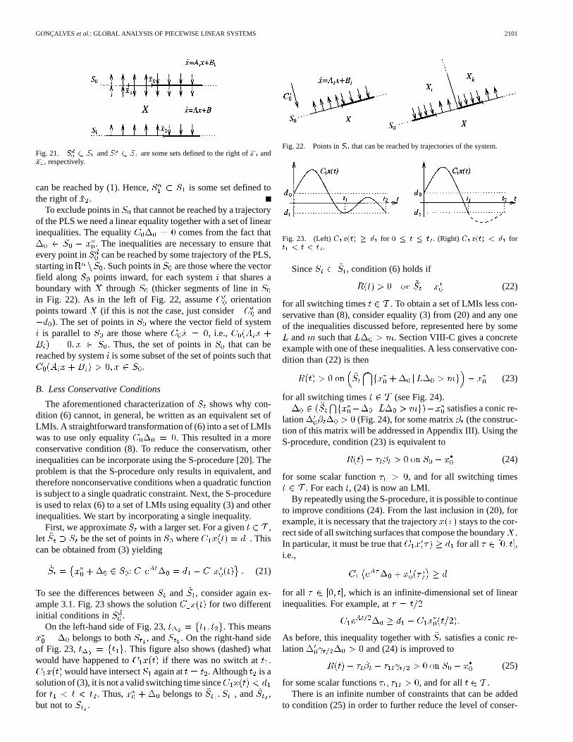
GONÇALVESet al.: GLOBAL ANALYSIS OF PIECEWISE LINEAR SYSTEMS 2101
Fig. 21. S � S andS � S are some sets defined to the right of�x and�x , respectively.
can be reached by (1). Hence, is some set defined tothe right of .
To exclude points in that cannot be reached by a trajectoryof the PLS we need a linear equality together with a set of linearinequalities. The equality comes from the fact that
. The inequalities are necessary to ensure thatevery point in can be reached by some trajectory of the PLS,starting in . Such points in are those where the vectorfield along points inward, for each systemthat shares aboundary with through (thicker segments of line inin Fig. 22). As in the left of Fig. 22, assume orientationpoints toward (if this is not the case, just consider and
). The set of points in where the vector field of systemis parallel to are those where , i.e.,
. Thus, the set of points in that can bereached by systemis some subset of the set of points such that
.
B. Less Conservative Conditions
The aforementioned characterization ofshows why con-dition (6) cannot, in general, be written as an equivalent set ofLMIs. A straightforward transformation of (6) into a set of LMIswas to use only equality . This resulted in a moreconservative condition (8). To reduce the conservatism, otherinequalities can be incorporate using the S-procedure [20]. Theproblem is that the S-procedure only results in equivalent, andtherefore nonconservative conditions when a quadratic functionis subject to a single quadratic constraint. Next, the S-procedureis used to relax (6) to a set of LMIs using equality (3) and otherinequalities. We start by incorporating a single inequality.
First, we approximate with a larger set. For a given ,let be the set of points in where . Thiscan be obtained from (3) yielding
(21)
To see the differences between and , consider again ex-ample 3.1. Fig. 23 shows the solution for two differentinitial conditions in .
On the left-hand side of Fig. 23, . This meansbelongs to both , and . On the right-hand side
of Fig. 23, . This figure also shows (dashed) whatwould have happened to if there was no switch at .
would have intersect again at . Although is asolution of (3), it is not a valid switching time sincefor . Thus, belongs to , and ,but not to .
Fig. 22. Points inS that can be reached by trajectories of the system.
Fig. 23. (Left)C x(t) � d for 0 � t � t . (Right)C x(t) < d fort < t < t .
Since , condition (6) holds if
(22)
for all switching times . To obtain a set of LMIs less con-servative than (8), consider equality (3) from (20) and any oneof the inequalities discussed before, represented here by some
and such that . Section VIII-C gives a concreteexample with one of these inequalities. A less conservative con-dition than (22) is then
(23)
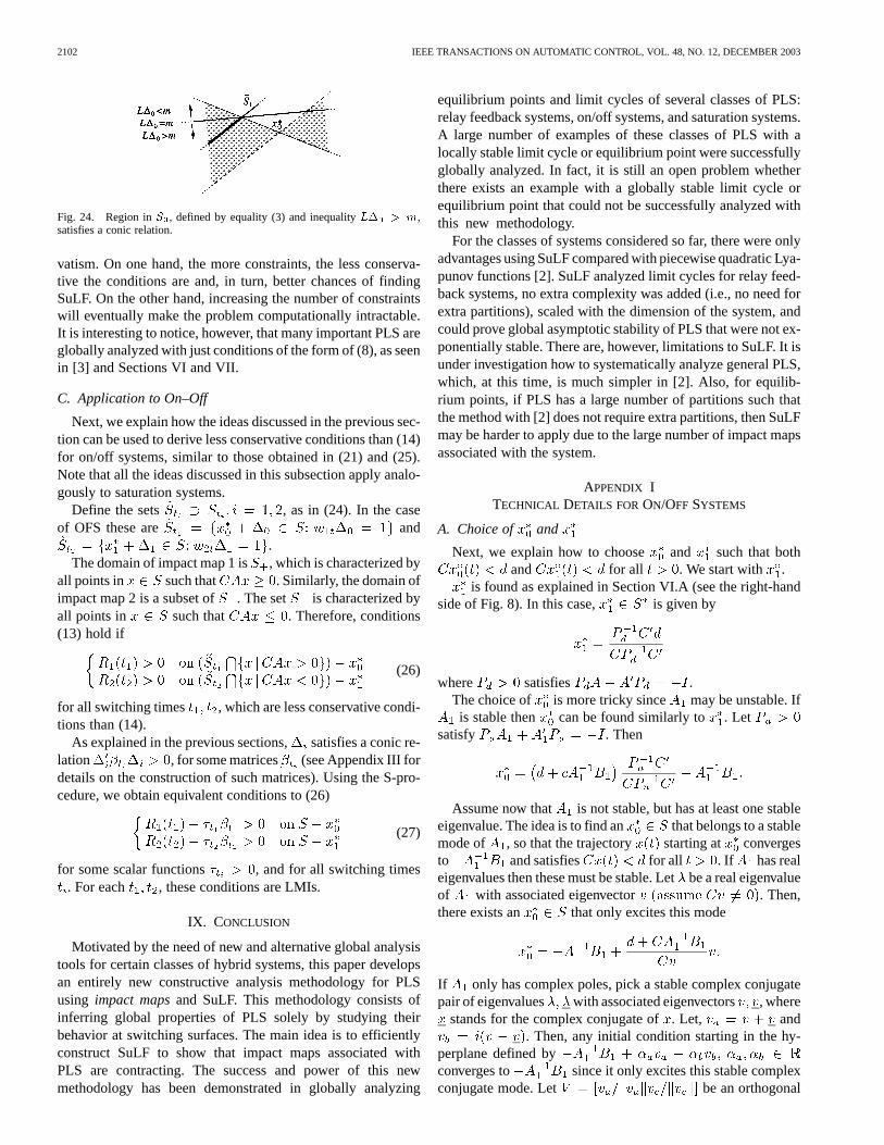
for all switching times (see Fig. 24).satisfies a conic re-
lation (Fig. 24), for some matrix (the construc-tion of this matrix will be addressed in Appendix III). Using theS-procedure, condition (23) is equivalent to
(24)
for some scalar function , and for all switching times. For each , (24) is now an LMI.
By repeatedly using the S-procedure, it is possible to continueto improve conditions (24). From the last inclusion in (20), forexample, it is necessary that the trajectory stays to the cor-rect side of all switching surfaces that compose the boundary.In particular, it must be true that for all ,i.e.,
for all , which is an infinite-dimensional set of linearinequalities. For example, at
As before, this inequality together with satisfies a conic re-lation and (24) is improved to
(25)
for some scalar functions , and for all .There is an infinite number of constraints that can be added
to condition (25) in order to further reduce the level of conser-
2102 IEEE TRANSACTIONS ON AUTOMATIC CONTROL, VOL. 48, NO. 12, DECEMBER 2003
Fig. 24. Region inS , defined by equality (3) and inequalityL� > m,satisfies a conic relation.
vatism. On one hand, the more constraints, the less conserva-tive the conditions are and, in turn, better chances of findingSuLF. On the other hand, increasing the number of constraintswill eventually make the problem computationally intractable.It is interesting to notice, however, that many important PLS areglobally analyzed with just conditions of the form of (8), as seenin [3] and Sections VI and VII.
C. Application to On–Off
Next, we explain how the ideas discussed in the previous sec-tion can be used to derive less conservative conditions than (14)for on/off systems, similar to those obtained in (21) and (25).Note that all the ideas discussed in this subsection apply analo-gously to saturation systems.
Define the sets , as in (24). In the caseof OFS these are and
.The domain of impact map 1 is , which is characterized by
all points in such that . Similarly, the domain ofimpact map 2 is a subset of . The set is characterized byall points in such that . Therefore, conditions(13) hold if
(26)
for all switching times , which are less conservative condi-tions than (14).
As explained in the previous sections, satisfies a conic re-lation , for some matrices (see Appendix III fordetails on the construction of such matrices). Using the S-pro-cedure, we obtain equivalent conditions to (26)
(27)
for some scalar functions , and for all switching times. For each , these conditions are LMIs.
IX. CONCLUSION
Motivated by the need of new and alternative global analysistools for certain classes of hybrid systems, this paper developsan entirely new constructive analysis methodology for PLSusing impact mapsand SuLF. This methodology consists ofinferring global properties of PLS solely by studying theirbehavior at switching surfaces. The main idea is to efficientlyconstruct SuLF to show that impact maps associated withPLS are contracting. The success and power of this newmethodology has been demonstrated in globally analyzing
equilibrium points and limit cycles of several classes of PLS:relay feedback systems, on/off systems, and saturation systems.A large number of examples of these classes of PLS with alocally stable limit cycle or equilibrium point were successfullyglobally analyzed. In fact, it is still an open problem whetherthere exists an example with a globally stable limit cycle orequilibrium point that could not be successfully analyzed withthis new methodology.
For the classes of systems considered so far, there were onlyadvantages using SuLF compared with piecewise quadratic Lya-punov functions [2]. SuLF analyzed limit cycles for relay feed-back systems, no extra complexity was added (i.e., no need forextra partitions), scaled with the dimension of the system, andcould prove global asymptotic stability of PLS that were not ex-ponentially stable. There are, however, limitations to SuLF. It isunder investigation how to systematically analyze general PLS,which, at this time, is much simpler in [2]. Also, for equilib-rium points, if PLS has a large number of partitions such thatthe method with [2] does not require extra partitions, then SuLFmay be harder to apply due to the large number of impact mapsassociated with the system.
APPENDIX ITECHNICAL DETAILS FOR ON/OFF SYSTEMS
A. Choice of and
Next, we explain how to choose and such that bothand for all . We start with .
is found as explained in Section VI.A (see the right-handside of Fig. 8). In this case, is given by
where satisfies .The choice of is more tricky since may be unstable. Ifis stable then can be found similarly to . Let
satisfy . Then
Assume now that is not stable, but has at least one stableeigenvalue. The idea is to find an that belongs to a stablemode of , so that the trajectory starting at convergesto and satisfies for all . If has realeigenvalues then these must be stable. Letbe a real eigenvalueof with associated eigenvector . Then,there exists an that only excites this mode
If only has complex poles, pick a stable complex conjugatepair of eigenvalues with associated eigenvectors , where
stands for the complex conjugate of. Let, and. Then, any initial condition starting in the hy-
perplane defined byconverges to since it only excites this stable complexconjugate mode. Let be an orthogonal
GONÇALVESet al.: GLOBAL ANALYSIS OF PIECEWISE LINEAR SYSTEMS 2103
basis in this plane, where . A trajectoryin this basis satisfies , where . Weneed to find an such that and
for all . This is a similarproblem to the one we dealt above when finding. In this case,
is given by
where satisfies . Finally,.
If only has complex unstable eigenvalues, then for anychoice of will have an infinity number of solu-tions for . In this case, must be chosen such that thesmallest solution of is higher than the max-imum possible switching time. Note that suchmay not exist.If that is the case, the linearization of the impact map must beparametrized by another variable at those values of where
, as explained in Section III.
B. Constraints Imposed When
Zero switching time corresponds to points insuch that. At those points, the SuLF must be continuous since
this is the only way both andcan be simultaneously satisfied, for all
such that and .Thus, at those points, , which is equivalentto . This imposes certain restrictionson , and . From Section VI-C,is given by
where , and
Let , and . Since ,then . This means that in the basis , thematrix must have the following structure:
for some and , where , with. Thus, once is fixed, must satisfy
. The same way , or. Hence, for some
. For a given is then given by
Finally, it must be true that leading to
In conclusion, the constraints imposed when reducethe free variable in conditions (13) and (14) to ,and .
C. Checking Stability Conditions for
Just like in RFS [3] and SAT, we would like to obtain boundson the set of switching times. With the exception of third-ordersystems, however, finding upper bounds on switchingtimes is, in general, not an easy task. The idea is to first guar-antee conditions (14) are satisfied in some intervalsand then check if they are also valid for all . Notethat and as . Thus, it isguaranteed that (13) and (14) are satisfied at since both
and .For simplicity, we present the case when . The other
cases follow analogously. Assume conditions (15) are satisfiedfor all . We would like to easily check if they willalso be satisfied for all . Consider first the secondcondition in (15). It is sufficient to show that
for all , and where . Next, we findan upper bound on the left-hand side of the last inequality. Let
. Since is a stable matrix, it is possible to finda and a such that . This inturn implies that , where is thesolution of with initial condition . Using the factthat
or, simply
Hence, for some
Therefore, we need to guarantee , with thelargest and smallest .
If is stable, a similar condition can be found analogouslyfor the first condition in (15). However, if (or if ) hasunstable complex poles, this approach will not work sinceis unbounded when . How to find bounds on switchingtimes for such systems of order higher than 3 is currently underinvestigation.
APPENDIX IITECHNICAL DETAILS FORSATURATION SYSTEMS: BOUNDS ON
SWITCHING TIMES
This section reduces checking (18) or (19) on some boundedset of switching times , instead of checking them forall possible switching times. In RFS [3], a bounded invariant setwhere all trajectories eventually enter and stay there was charac-terized. Bounds on the switching times of trajectories inside that
2104 IEEE TRANSACTIONS ON AUTOMATIC CONTROL, VOL. 48, NO. 12, DECEMBER 2003
bounded invariant set were found. The same ideas can be usedfor SAT whenever is Hurwitz since is a boundedinput.
First, notice that since the associated impactmaps are defined on the same switching surface and are allowedto have zero switching time. Analysis of impact maps 1 andat imposes the same constraints on the parameters of theLyapunov functions as in OFS. See Appendix I.B for details.
As for impact map , zero switching never occurssince there is a “gap” betweenand , resulting in a nonzeroswitching time for every trajectory starting in . For certainlarge values of , the switching times can be made arbitrarilysmall. In the invariant bounded set described above, however,switching times for impact map cannot be made arbitrarilysmall, and a lower bound can be found. Using the sameideas, upper bounds on switching times for all impact mapscan be found. Bounds on switching times for the case wherehas unstable imaginary eigenvalues can be found as explainedin Example 7.3.
Before finding bounds on switching times, we need to char-acterize a bounded set such that any trajectory will eventuallyenter and stay there. The following proposition is similar to [3,Prop. 7.1]. Thus, the proof is omitted here.
Proposition 3: Consider the system ,where is Hurwitz, , and is a row vector. Then
Remember that, by definition, is given by
As a remark, if and , it fol-lows the origin is globally asymptotically stable. When
, eventually all trajectories enter andremain in the set , where the system is linear andstable. Note that this remark also follows from the well knownsmall-gain theorem.
We first focus our attention on upper bounds of the switchingtimes , starting with . A trajectory starting at
is given by . Thus, theoutput is given by
Since and Hurwitz, cannot remainlarger than for all . For any initial condition
as , which meansfor some . Thus, a switch must occur in finite time. Since fora sufficiently large enough time enters a bounded in-variant set (from the above proposition), an upper bound on thisswitching time can be obtained. The following propositionis similar to [3, Prop. 7.2].
Proposition 4: Let be the smallest solution of
If and are sufficiently large consecutive switching times ofthe first impact map then .
Next, we find upper bounds on the switching times of impactmaps and . The idea here is to find the minimumsuch that , for all and all inthe bounded invariant set. In this derivation, .
Proposition 5: Let be the smallest solution of
(28)
If and are sufficiently large consecutive switching times ofimpact maps or , then , and .
We now focus on the lower bound on the switching timesof impact map , i.e, . Remember that if , then
. Since , it must be true that at leastin some interval . Basically, the time it takes to go fromto must always be nonzero. The next result shows that when atrajectory enters the bounded invariant set characterized before,
cannot be made arbitrarily small. Thus, a lower bound on thetime it takes between two consecutive switches fromto canbe obtained.
Proposition 6: Let , andand define .
Let . If and are sufficientlylarge consecutive switching times of impact map, then
.The proof is similar to the proof of [3, Prop. 7.3].
APPENDIX IIICONSTRUCTION OFCONIC RELATIONS
We now describe how to construct the conesintroduced inSection VIII-B. For each , the cone is defined by two hy-perplanes in : one is the hyperplane parallel to containing
and the other is the hyperplane defined by the intersectionof and , and con-taining the point (see Fig. 24). Let and , respec-tively, be vectors in perpendicular to each hyperplane. Oncethese vectors are known, the cone can easily be characterized.This is composed of all the vectors such that
. The symmetric matrix intro-duced in (24) is just where .Remember that the cone is centered atand note that afteris chosen, must have the right direction in order to guarantee
.We first find , the vector perpendicular to . Looking
back at the definition of is given by
The derivation of is not as trivial as . We actually need tointroduce a few extra variables. The first one is , the vectorperpendicular to the set , given by .
Proposition 7: The hyperplane defined by the intersection ofand , and containing the point is perpendicular to the
vector
GONÇALVESet al.: GLOBAL ANALYSIS OF PIECEWISE LINEAR SYSTEMS 2105
Proof: can be parameterize the following way:
and
The intersection of and occurs at points in such that. Multiplying on the left by we have
or
(29)
We want to show that
Using (29), we have
The characterization of is not complete yet. The orientationof must be carefully chosen to guarantee that the conecontains .
Proposition 8: If
then the cone contains.
The proof, omitted here, is based on taking a pointand showing that .
REFERENCES
[1] M. S. Branicky, “Studies in hybrid systems: modeling, analysis, andcontrol,” Ph.D. dissertation, Mass. Inst. Technol., Cambridge, MA,1995.
[2] M. Johansson and A. Rantzer, “Computation of piecewise quadratic Lya-punov functions for hybrid systems,”IEEE Trans. Automat. Contr., vol.43, pp. 555–559, Apr. 1998.
[3] J. M. Gonçalves, A. Megretski, and M. A. Dahleh, “Global stabilityof relay feedback systems,”IEEE Trans. Automat. Contr., vol. 46, pp.550–562, Apr. 2001.
[4] G. Zames and P. L. Falb, “Stability conditions for systems with mono-tone and slope-restricted nonlinearities,” inSIAM J. Control, vol. 6,1968, pp. 89–108.
[5] F. D’Amato, A. Megretski, U. Jönsson, and M. Rotea, “Integral quadraticconstraints for monotonic and slope-restricted diagonal operators,” inProc. Amer. Control Conf., San Diego, CA, June 1999, pp. 2375–2379.
[6] U. Jönsson and A. Megretski, “The Zames–Falb IQC for systems withintegrators,”IEEE Trans. Automat. Contr., vol. 45, pp. 560–565, Mar.2000.
[7] A. Megretski, “New IQC for quasiconcave nonlinearities,” presented atthe Amer. Control Conf., San Diego, CA, June 1999.
[8] A. Megretski and A. Rantzer, “System analysis via integral quadraticconstrains,”IEEE Trans. Automat. Contr., vol. 42, pp. 819–830, June1997.
[9] J. M. Gonçalves, “L -gain of double integrators with saturation non-linearity,” IEEE Trans. Automat. Contr., vol. 47, pp. 2063–2068, Dec.2002.
[10] , “Constructive global analysis of hybrid systems,” M.S. thesis,Mass. Inst. Technol., Cambridge, MA, Sept. 2000.
[11] S. Pettersson and B. Lennartson, “An LMI approach for stability analysisof nonlinear systems,” presented at the Eur. Control Conf., Brussels,Belgium, July 1997.
[12] A. Hassibi and S. Boyd, “Quadratic stabilization and control of piece-wise linear systems,” presented at the Amer. Control Conf., Philadel-phia, PA, 1998.
[13] H. K. Khalil, Nonlinear Systems, 2nd ed. Upper Saddle River, NJ:Prentice-Hall, 1996.
[14] P. A. Parrilo, “Structured Semidefinite Programs and semialgebraicgeometry methods in robustness and optimization,” Ph.D. dissertation,California Inst. Technol., Pasadena, CA, 2000.
[15] Web Page. [Online]. Available: http://www.cds.caltech.edu/~jmg/[16] A. Saberi, Z. Lin, and A. Teel, “Control of linear systems with satu-
rating actuators,”IEEE Trans. Automat. Contr., vol. 41, pp. 368–378,Mar. 1996.
[17] H. J. Sussmann, E. D. Sontag, and Y. Yang, “A general result on the sta-bilization of linear systems using bounded controls,”IEEE Trans. Au-tomat. Contr., vol. 39, pp. 2411–2425, Dec. 1994.
[18] A. R. Teel, “A nonlinear small gain theorem for the analysis of con-trol systems with saturation,”IEEE Trans. Automat. Contr., vol. 41, pp.1256–1270, Sept. 1996.
[19] R. Suárez, J. Alvarez, and J. Alvarez, “Linear systems with single sat-urated input: Stability analysis,” presented at the 30th Conf. DecisionControl, Brighton, U.K., Dec. 1991.
[20] S. Boyd, L. El Ghaoui, E. Feron, and V. Balakrishnan,Linear MatrixInequalities in System and Control Theory. Philadelphia, PA: SIAM,1994.
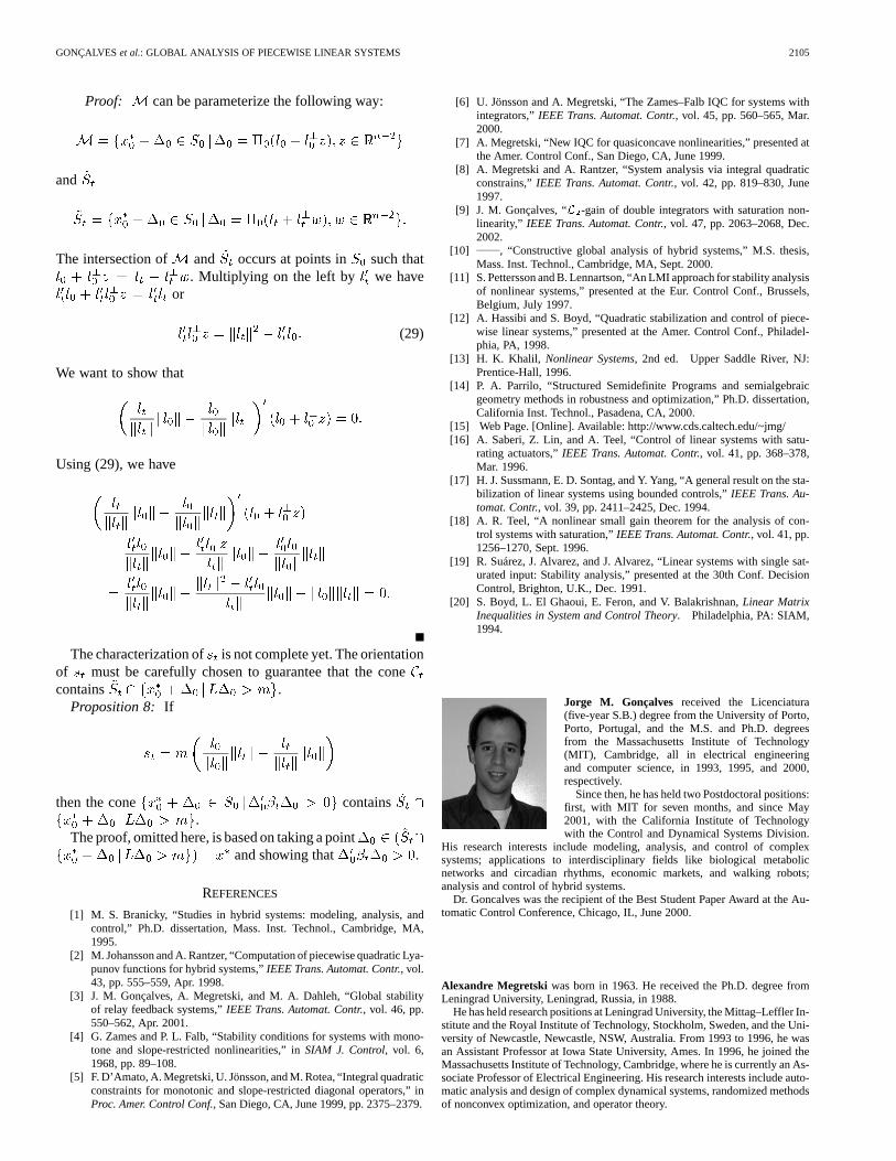
Jorge M. Gonçalves received the Licenciatura(five-year S.B.) degree from the University of Porto,Porto, Portugal, and the M.S. and Ph.D. degreesfrom the Massachusetts Institute of Technology(MIT), Cambridge, all in electrical engineeringand computer science, in 1993, 1995, and 2000,respectively.
Since then, he has held two Postdoctoral positions:first, with MIT for seven months, and since May2001, with the California Institute of Technologywith the Control and Dynamical Systems Division.
His research interests include modeling, analysis, and control of complexsystems; applications to interdisciplinary fields like biological metabolicnetworks and circadian rhythms, economic markets, and walking robots;analysis and control of hybrid systems.
Dr. Goncalves was the recipient of the Best Student Paper Award at the Au-tomatic Control Conference, Chicago, IL, June 2000.
Alexandre Megretski was born in 1963. He received the Ph.D. degree fromLeningrad University, Leningrad, Russia, in 1988.
He has held research positions at Leningrad University, the Mittag–Leffler In-stitute and the Royal Institute of Technology, Stockholm, Sweden, and the Uni-versity of Newcastle, Newcastle, NSW, Australia. From 1993 to 1996, he wasan Assistant Professor at Iowa State University, Ames. In 1996, he joined theMassachusetts Institute of Technology, Cambridge, where he is currently an As-sociate Professor of Electrical Engineering. His research interests include auto-matic analysis and design of complex dynamical systems, randomized methodsof nonconvex optimization, and operator theory.
2106 IEEE TRANSACTIONS ON AUTOMATIC CONTROL, VOL. 48, NO. 12, DECEMBER 2003
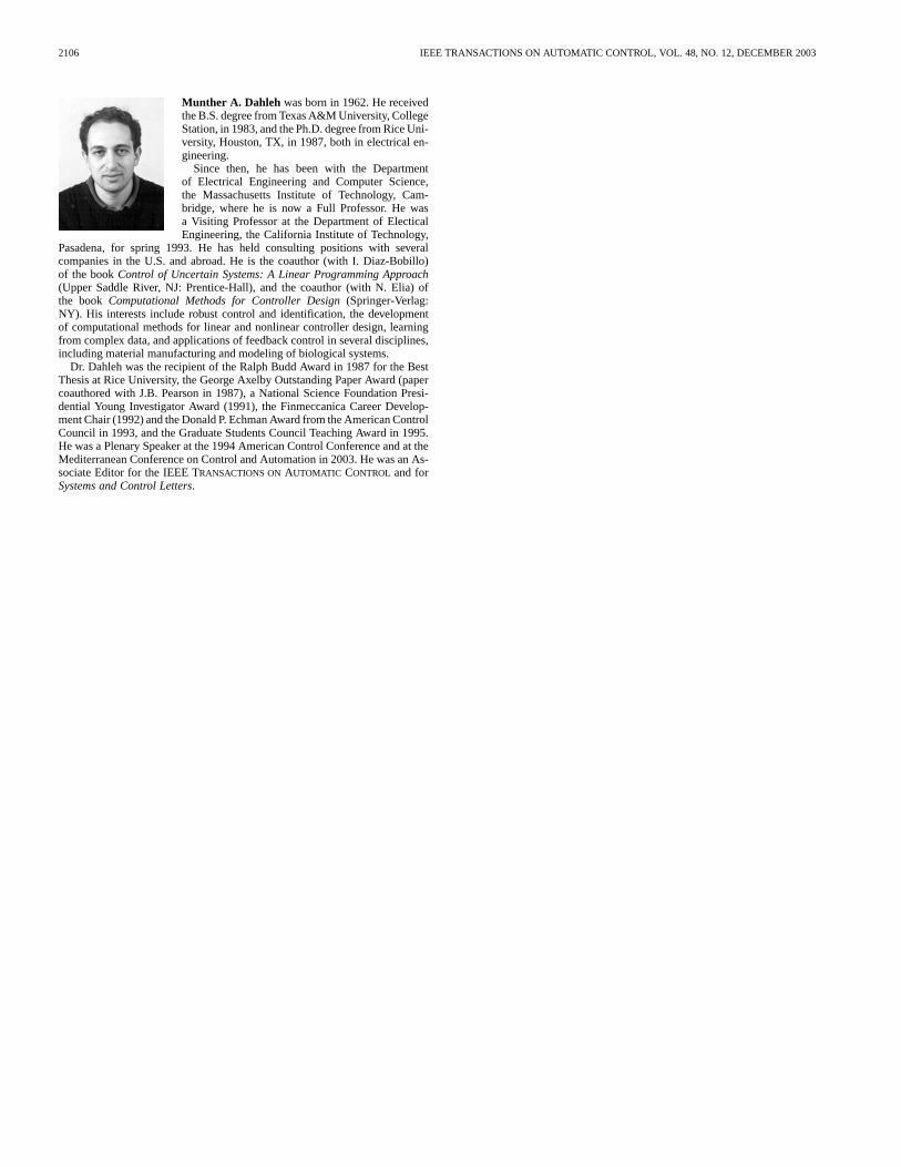
Munther A. Dahleh was born in 1962. He receivedthe B.S. degree from Texas A&M University, CollegeStation, in 1983, and the Ph.D. degree from Rice Uni-versity, Houston, TX, in 1987, both in electrical en-gineering.
Since then, he has been with the Departmentof Electrical Engineering and Computer Science,the Massachusetts Institute of Technology, Cam-bridge, where he is now a Full Professor. He wasa Visiting Professor at the Department of ElecticalEngineering, the California Institute of Technology,
Pasadena, for spring 1993. He has held consulting positions with severalcompanies in the U.S. and abroad. He is the coauthor (with I. Diaz-Bobillo)of the bookControl of Uncertain Systems: A Linear Programming Approach(Upper Saddle River, NJ: Prentice-Hall), and the coauthor (with N. Elia) ofthe book Computational Methods for Controller Design(Springer-Verlag:NY). His interests include robust control and identification, the developmentof computational methods for linear and nonlinear controller design, learningfrom complex data, and applications of feedback control in several disciplines,including material manufacturing and modeling of biological systems.
Dr. Dahleh was the recipient of the Ralph Budd Award in 1987 for the BestThesis at Rice University, the George Axelby Outstanding Paper Award (papercoauthored with J.B. Pearson in 1987), a National Science Foundation Presi-dential Young Investigator Award (1991), the Finmeccanica Career Develop-ment Chair (1992) and the Donald P. Echman Award from the American ControlCouncil in 1993, and the Graduate Students Council Teaching Award in 1995.He was a Plenary Speaker at the 1994 American Control Conference and at theMediterranean Conference on Control and Automation in 2003. He was an As-sociate Editor for the IEEE TRANSACTIONS ONAUTOMATIC CONTROL and forSystems and Control Letters.


