PHYSICAL REVIEW E 91, 032301 (2015)

Anisotropic stress correlations in two-dimensional liquids

Bin Wu,1 Takuya Iwashita,2 and Takeshi Egami1,2,3,*

1Department of Physics and Astronomy, Joint Institute of Neutron Science, University of Tennessee, Knoxville, Tennessee 37996, USA2Department of Materials Science and Engineering, University of Tennessee, Knoxville, Tennessee 37996, USA

3Oak Ridge National Laboratory, Oak Ridge, Tennessee 37831, USA(Received 5 November 2014; published 2 March 2015)

In this paper we demonstrate the presence of anisotropic stress correlations in the simulated two-dimensionalliquids. Whereas the temporal correlation of macroscopic shear stress is known to contribute to viscosity via theGreen-Kubo formula, the general question regarding angular dependence of the spatial correlation among atomic-level stresses in liquids without external shear has not been explored. We observed the apparent anisotropicity withwell-defined symmetry which can be explained in terms of the elastic continuum theory by Eshelby. In addition,we found that the shear stress correlation is screened compared to the prediction by the elastic continuum theory,and the screening length depends on temperature and follows the power law, suggesting divergence around theglass transition temperature. The success of the Eshelby theory to explain the anisotropy of the stress correlationsjustifies the idea that the mismatch between the atom and its nearest neighbor cage produces the atomic-levelstress as well as the long-range stress fields.

DOI: 10.1103/PhysRevE.91.032301 PACS number(s): 64.70.Q−, 64.70.kj, 05.10.−a, 05.20.Jj

I. INTRODUCTION

A liquid shows time-dependent response to external shearstress, with the characteristic time scale of the Maxwellrelaxation time, τM = η/G∞, where η is viscosity and G∞is the high-frequency shear modulus [1]. If the time scale ofexperiment is longer than τM the liquid offers no resistance, butif it is shorter the liquid behaves like a solid with the elasticmodulus similar to that of the crystalline solid made of thesame chemical composition. Therefore a liquid can sustain aninternal stress field for a time scale of τM . Indeed the viscosityis related to the temporal correlation of macroscopic shearstress through the Green-Kubo equation,

η = V

kT

∫ ∞

0〈σxy (0) σxy (t)〉dt, (1)

where V is the sample volume, σxy(t) is the shear stress inthe x-y plane at time t , k is the Boltzmann constant, and T istemperature [1]. The total shear stress in Eq. (1) can be brokeninto contributions from individual atoms thereby leading to thefollowing expression [2,3]:

η = 1

kT V

∫ ∞

0

⟨∑i,j

Viσxy

i (0) Vjσxy

j (t)

⟩dt, (2)

where Vi and σxy

i are the atomic volume and the atomic-level stress of the ith atom. Hence the viscosity implicitlyintegrates spatiotemporal correlations of atomic-level stresses.Levashov et al. [3] investigated the role of correlation lengthin the viscosity calculation and concluded that the viscosityis a nonlocal parameter. However, the angular dependenceof stress correlations was not explored in their study, where

*Author to whom correspondence should be addressed:egami@utk.edu

the correlation function was averaged spherically over relativedistance between two particles, i.e., |−→ri − −→

rj |.In this article we study the anisotropy of spatial stress corre-

lations in high-temperature liquids. A simple two-dimensional(2D) colloidal liquid interacting with the screened Coulombpotential is simulated using classical molecular dynamics(MD) [4] for this purpose because the physics is the same forcolloidal liquids as well as atomic liquids, and the anisotropyis more readily demonstrated in 2D. It is found that the com-puted correlation functions are distinctively anisotropic andcharacterized by well-defined twofold or fourfold symmetriesdepending on the elements of the stress tensor. In order toidentify the underlying mechanism of the observed anisotropy,we explain the simulation results in terms of Eshelby’stheory of inclusion [5]. This theory was originally developedwithin the framework of continuum elasticity and solves theproblem where a region (“inclusion”) undergoes deformationconstrained by its surroundings (“matrix”). For instance, whenan elliptical subject is squeezed into a spherical hole, Eshelby’stheory predicts a long-ranged and anisotropic elastic fieldoutside the hole, i.e., in the matrix. Recently more studieshave been reported on the applicability of Eshelby’s theoryin amorphous materials concerning their plasticity [6–25].Different from previous reports that focused on supercooledliquids [6], glasses [7,9–20,22,23], or colloids [24,25] underexternal perturbation, e.g., shear, the present work extendsthe idea to high-temperature liquids in equilibrium without anapplied stress by using the concept of the atomic-level stresses.

The rest of this paper is organized as follows. In Sec. II, wedescribe our MD simulation setup and data analysis methodsused to identify the boundary of liquid phase and to calculatestress correlation functions. In Sec. III, we first demonstratethat the spatial stress correlation functions in two-dimensional(2D) liquids are distinctively anisotropic. Then we investigatethe nature of their oscillations and temperature-dependentamplitudes. In Sec. IV, we present the stress fields calculatedusing Eshelby’s theory and compare their symmetries withthose of the simulation results. We summarize conclusions inSec. V.

1539-3755/2015/91(3)/032301(10) 032301-1 ©2015 American Physical Society

BIN WU, TAKUYA IWASHITA, AND TAKESHI EGAMI PHYSICAL REVIEW E 91, 032301 (2015)

II. MOLECULAR DYNAMICS SIMULATION

A. Simulation setup

We used the LAMMPS code [26] to carry out two-dimensional molecular dynamics simulations. The setup issimilar to the one reported in Refs. [27,28]. We considera monoatomic system interacting through pairwise Yukawapotential [29]. This potential has been successful in describingthe interaction between charged colloids, e.g., dendrimers [30].Its mathematical expression is presented below:

V (r) = U0σ

rexp

(−λ

r − σ

σ

), (3)

where U0 defines the strength of the interaction, λ is thescreening parameter, σ is the size of a particle, and r representsthe interparticle distance. With employment of reduced unitformalism, we kept U0 = 1, σ = 1, Boltzmann constant k = 1,and the mass of a particle m = 1 throughout the simulations.Moreover, we set λ = 8 and the cutoff distance for force evalu-ation as 4.1. We used a rectangular simulation box and appliedperiodic boundary condition on both directions. The ratio ofthe lengths of two sides is 2 :

√3 for the sake of minimizing

box size effect [27,28,31]. All simulation runs were performedunder canonical ensemble while the temperature control wasachieved by Nose-Hoover thermostat. The number of particlesN = 2500, the area of simulation box A = 2173.91, andtherefore the number density ρ = N

A= 1.15. The time step

for integrating equations of motion via the Verlet algorithmis 0.005 in reduced unit. We used the triangular crystallinelattice as the initial structure and gradually heated the systemto each of the temperatures of interest. We waited 107 timesteps after the targeted temperature was reached and thencollected 104 frames of trajectories, which were 103 time stepsapart. The Maxwell relaxation time deduced from temporalcorrelation of macroscopic shear stress ranges from 0.2985 to0.0512 (approximately 60 and 10 MD steps, respectively) atthe studied temperatures of 1 to 7 in liquid phase. Hence onecan realize that the system is truly in equilibrium before thedata collection.

B. Phase behavior

We use the potential energy per atom, Ea , to qualitativelymonitor the phase behavior of the system under study. Thisquantity can be computed via the following equation:

Ea =⟨

1

2N

∑i

∑j �=i

V (rij )

⟩. (4)

The results are presented in Fig. 1 as a function of thereduced temperature T ∗. At low temperatures the systemis expected to be stable in the crystalline phase where Ea

increases linearly with T ∗. As the temperature approachesapproximately 0.9, the system starts to melt, signified by theemergence of the steep slope. The system ultimately enters theliquid phase at a temperature around 1.0, where Ea resumeslinear dependence on T ∗.

There has been an ongoing debate over the meltingmechanism in two dimensions. On one hand, the Kosterlitz-Thouless-Halperin-Nelson-Young (KTHNY) theory [32–35]

FIG. 1. Potential energy per atom as a function of reducedtemperature. The divergence from linearity at temperature around0.9 suggests onset of melting process while its recurrence around 1.0indicates entrance to liquid phase.

predicts that the system can experience a hexatic phase in itspath of transformation from a crystal to a liquid. The signatureof this hexatic phase is the quasi-long-range orientationalorder. On the other hand, 2D melting is believed to be a simplefirst-order phase transition [36]. There have been extensivestudies to support both sides. Since deciphering the meltingprocess is not the primary interest of the present study, wefocus on identifying the boundary of liquid phase using thebond orientational-order parameter.

Taking the x axis as the reference axis, the bond anglebetween the particle k and each of its nearest neighbors j

can be defined. The angle θkj should satisfy the cos(6θkj ) = 1condition in the perfect crystalline phase and gradually divergefrom it statistically as temperature increases. Hence the localbond angular order is quantified by

�6 (r) = 1

Nk

Nk∑j=1

ei6θkj , (5)

where Nk represents the number of nearest neighbors of theparticle k. Its autocorrelation function, which is defined byEq. (6), provides a measure of the range of the orientationalorder.

g6 (r) = 〈�∗6 (r) �6 (0)〉. (6)

Figure 2 illustrates g6(r) at temperatures in the vicinity ofthe melting point. In the crystalline phase, g6(r) converges toa finite asymptotic value which indicates the presence of long-range orientational order. A possible hexatic phase is foundat T ∗ = 0.95, where g6(r) decays algebraically suggesting aquasi-long-range order of bond orientation exists in the system.As soon as the particles form liquids, the asymptotic form ofg6(r) changes to an exponential decay over r . Therefore, thesystem is indeed in the liquid phase at T ∗ � 1.

032301-2

ANISOTROPIC STRESS CORRELATIONS IN TWO- . . . PHYSICAL REVIEW E 91, 032301 (2015)

FIG. 2. (Color online) Spatial correlation function of bondorientational-order parameter at T ∗ = 0.9 (top black line), T ∗ = 0.95(upper middle green line), T ∗ = 1.0 (lower middle pink line), andT ∗ = 1.1 (bottom dark red line). g6(r) converges to a finite valueonly at crystalline phase while it decays algebraically at hexatic phaseand exponentially at liquid phase. Hence the phase behavior at eachpresented temperature is readily identified.

C. Atomic-level stress tensor

We assess the stresses at each particle via the atomic-levelstress [2], which can be computed from

σαβ

i = 1

2Ai

∑j

1

rij

dV (rij )

drrαij r

β

ij , (7)

where α and β indicate the corresponding Cartesian compo-nent while the summation runs over all particles residing insidethe circle centered at the particle i with the radius being thecutoff distance set for MD simulation. Ai is the atomic areathat can be evaluated using the Voronoi polyhedra. However,for the sake of simplicity, this work replaces it with the averageatomic area defined by Aave = A

N, where A is the total area of

the simulation box.

D. Spatial stress correlation functions

The spatial stress correlation functions are the most impor-tant quantities in the present study. The functions correlate onecomponent or some combinations of the elements in the stresstensor of one particle with that (those) of others. We presentthe spatial x-y shear stress correlation function as one example,which takes the following expression:

Cs1,s1(r) =˝∑

i

∑j �=i σ s1

i σ s1j δ(r − −→

ri + −→rj )√∑

i

(σ s1

i

)2√∑

j

(σ s1

j

)2

˛, (8)

where σ s1 = σxy . It is important to note that the angulardependence of this correlation function is preserved in contrastto g6(r). We will show below the elastic fields are characterizedby 4θ or 2θ symmetries, where θ is the polar angle. Inaddition to the x-y shear stress, we also consider the hydrostaticpressure, p = (σxx + σyy)/2, as well as the other shear stress,σ s2 = (σxx − σyy)/2, for auto- and cross correlations. We notethat the hydrostatic pressure of each particle is subtracted byits ensemble average value, which accounts for the externalpressure applied to keep the volume of the system constant, inthe correlation analysis.

III. STRESS CORRELATIONS IN LIQUIDS

In this section, we illustrate the existence of anisotropiccorrelations among the atomic-level stresses in the 2D Yukawaliquids. The correlation functions are characterized by well-defined 4θ or 2θ symmetry which resembles the stress patternin the matrix induced by a circular inclusion to be introducedlater. We then examine the nature of their oscillations andtemperature-dependent amplitudes.

A. Symmetry

In Fig. 3, we present the spatial autocorrelation of the x-yshear stress computed at temperature T ∗ = 1. In Fig. 3(a) thescale of the color scheme matches the maximum intensity ofthe correlation function. One clearly sees four bright spotsnear the center due to the nearest neighbors overshadowingthe rest, each of which takes one corner of the diagonals. Thefourfold symmetry is evident. For clear visualization of the farfield we rescaled the color scheme in Fig. 3(b). The innermost

FIG. 3. (Color) The spatial shear stress correlation function computed at T ∗ = 1. In panel (a), the scale of the color scheme matches theintensity of the correlation function while in panel (b) the scale is set to highlight a remote area.

032301-3

BIN WU, TAKUYA IWASHITA, AND TAKESHI EGAMI PHYSICAL REVIEW E 91, 032301 (2015)

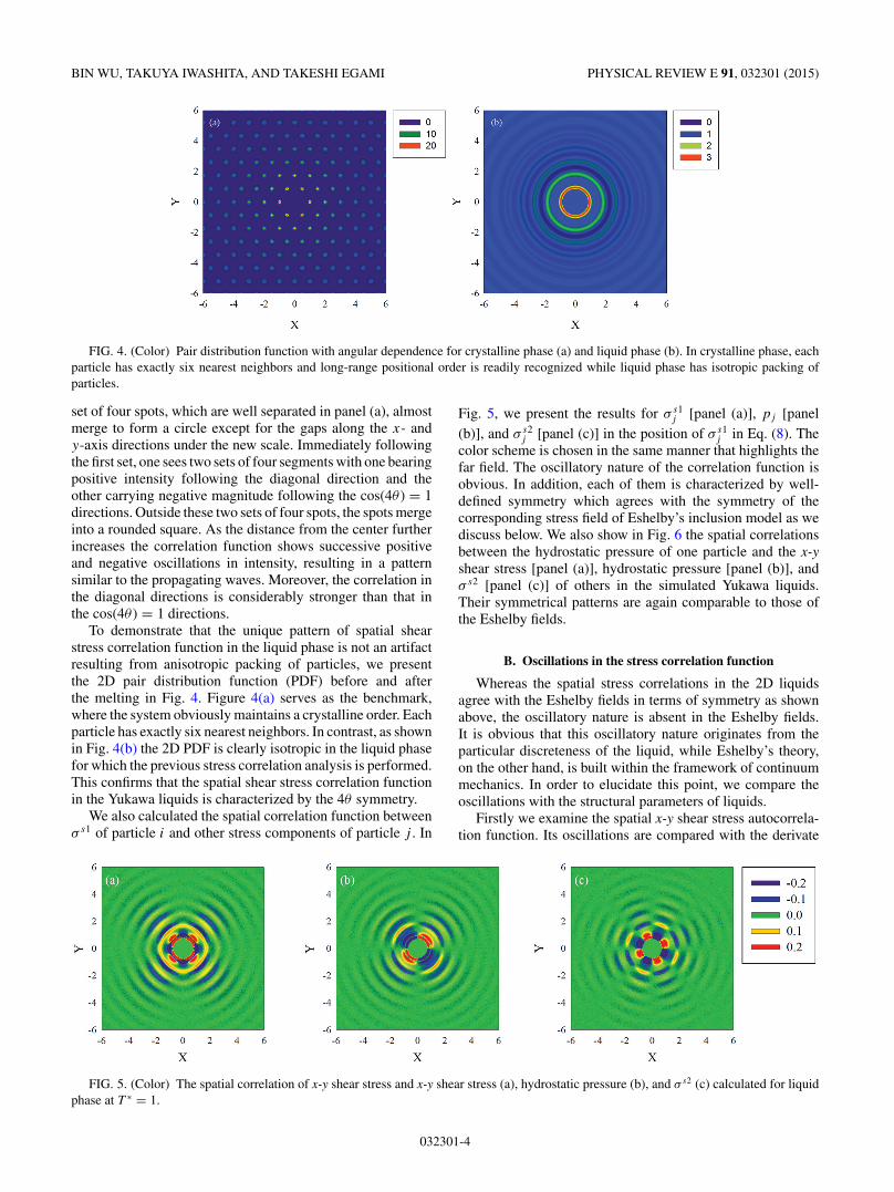
FIG. 4. (Color) Pair distribution function with angular dependence for crystalline phase (a) and liquid phase (b). In crystalline phase, eachparticle has exactly six nearest neighbors and long-range positional order is readily recognized while liquid phase has isotropic packing ofparticles.

set of four spots, which are well separated in panel (a), almostmerge to form a circle except for the gaps along the x- andy-axis directions under the new scale. Immediately followingthe first set, one sees two sets of four segments with one bearingpositive intensity following the diagonal direction and theother carrying negative magnitude following the cos(4θ ) = 1directions. Outside these two sets of four spots, the spots mergeinto a rounded square. As the distance from the center furtherincreases the correlation function shows successive positiveand negative oscillations in intensity, resulting in a patternsimilar to the propagating waves. Moreover, the correlation inthe diagonal directions is considerably stronger than that inthe cos(4θ ) = 1 directions.

To demonstrate that the unique pattern of spatial shearstress correlation function in the liquid phase is not an artifactresulting from anisotropic packing of particles, we presentthe 2D pair distribution function (PDF) before and afterthe melting in Fig. 4. Figure 4(a) serves as the benchmark,where the system obviously maintains a crystalline order. Eachparticle has exactly six nearest neighbors. In contrast, as shownin Fig. 4(b) the 2D PDF is clearly isotropic in the liquid phasefor which the previous stress correlation analysis is performed.This confirms that the spatial shear stress correlation functionin the Yukawa liquids is characterized by the 4θ symmetry.

We also calculated the spatial correlation function betweenσ s1 of particle i and other stress components of particle j . In

Fig. 5, we present the results for σ s1j [panel (a)], pj [panel

(b)], and σ s2j [panel (c)] in the position of σ s1

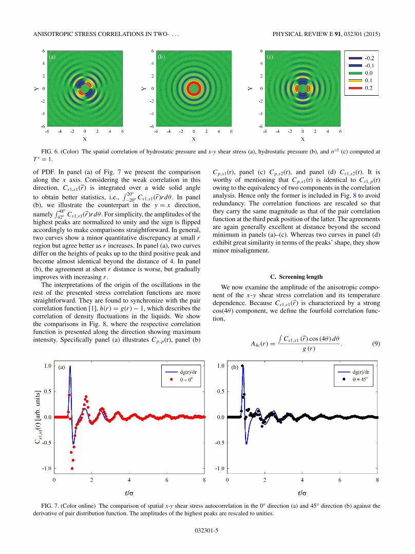
j in Eq. (8). Thecolor scheme is chosen in the same manner that highlights thefar field. The oscillatory nature of the correlation function isobvious. In addition, each of them is characterized by well-defined symmetry which agrees with the symmetry of thecorresponding stress field of Eshelby’s inclusion model as wediscuss below. We also show in Fig. 6 the spatial correlationsbetween the hydrostatic pressure of one particle and the x-yshear stress [panel (a)], hydrostatic pressure [panel (b)], andσ s2 [panel (c)] of others in the simulated Yukawa liquids.Their symmetrical patterns are again comparable to those ofthe Eshelby fields.

B. Oscillations in the stress correlation function

Whereas the spatial stress correlations in the 2D liquidsagree with the Eshelby fields in terms of symmetry as shownabove, the oscillatory nature is absent in the Eshelby fields.It is obvious that this oscillatory nature originates from theparticular discreteness of the liquid, while Eshelby’s theory,on the other hand, is built within the framework of continuummechanics. In order to elucidate this point, we compare theoscillations with the structural parameters of liquids.

Firstly we examine the spatial x-y shear stress autocorrela-tion function. Its oscillations are compared with the derivate

FIG. 5. (Color) The spatial correlation of x-y shear stress and x-y shear stress (a), hydrostatic pressure (b), and σ s2 (c) calculated for liquidphase at T ∗ = 1.

032301-4

ANISOTROPIC STRESS CORRELATIONS IN TWO- . . . PHYSICAL REVIEW E 91, 032301 (2015)

FIG. 6. (Color) The spatial correlation of hydrostatic pressure and x-y shear stress (a), hydrostatic pressure (b), and σ s2 (c) computed atT ∗ = 1.

of PDF. In panel (a) of Fig. 7 we present the comparisonalong the x axis. Considering the weak correlation in thisdirection, Cs1,s1(r) is integrated over a wide solid angleto obtain better statistics, i.e.,

∫ 20o

−20o Cs1,s1(r)rdθ . In panel(b), we illustrate the counterpart in the y = x direction,namely

∫ 48o

42o Cs1,s1(r)rdθ . For simplicity, the amplitudes of thehighest peaks are normalized to unity and the sign is flippedaccordingly to make comparisons straightforward. In general,two curves show a minor quantitative discrepancy at small r

region but agree better as r increases. In panel (a), two curvesdiffer on the heights of peaks up to the third positive peak andbecome almost identical beyond the distance of 4. In panel(b), the agreement at short r distance is worse, but graduallyimproves with increasing r .

The interpretations of the origin of the oscillations in therest of the presented stress correlation functions are morestraightforward. They are found to synchronize with the paircorrelation function [1], h(r) = g(r) − 1, which describes thecorrelation of density fluctuations in the liquids. We showthe comparisons in Fig. 8, where the respective correlationfunction is presented along the direction showing maximumintensity. Specifically panel (a) illustrates Cp,p(r), panel (b)

Cp,s1(r), panel (c) Cp,s2(r), and panel (d) Cs1,s2(r). It isworthy of mentioning that Cp,s1(r) is identical to Cs1,p(r)owing to the equivalency of two components in the correlationanalysis. Hence only the former is included in Fig. 8 to avoidredundancy. The correlation functions are rescaled so thatthey carry the same magnitude as that of the pair correlationfunction at the third peak position of the latter. The agreementsare again generally excellent at distance beyond the secondminimum in panels (a)–(c). Whereas two curves in panel (d)exhibit great similarity in terms of the peaks’ shape, they showminor misalignment.

C. Screening length

We now examine the amplitude of the anisotropic compo-nent of the x-y shear stress correlation and its temperaturedependence. Because Cs1,s1(r) is characterized by a strongcos(4θ ) component, we define the fourfold correlation func-tion,

A4c(r) =∫

Cs1,s1 (r) cos (4θ ) dθ

g (r). (9)

FIG. 7. (Color online) The comparison of spatial x-y shear stress autocorrelation in the 0° direction (a) and 45° direction (b) against thederivative of pair distribution function. The amplitudes of the highest peaks are rescaled to unities.

032301-5

BIN WU, TAKUYA IWASHITA, AND TAKESHI EGAMI PHYSICAL REVIEW E 91, 032301 (2015)

FIG. 8. (Color online) The comparison between oscillations of Cp,p(r) (a), Cp,s1(r) (b), Cp,s2(r) (c), and Cs1,s2(r) (d) along respectivemaximum intensity directions and that of pair correlation function, h(r). The correlation functions are rescaled to share the same amplitudewith pair correlation function at the third peak position of the latter, i.e., r = 2.68.

FIG. 9. (Color online) The cos(4θ ) component of spatial x-y shear stress autocorrelation function computed at T ∗ = 1. Panel (a) presentsthe result in linear scale and panel (b) shows its absolute value in logarithmic scale along with a fitting curve.

032301-6

ANISOTROPIC STRESS CORRELATIONS IN TWO- . . . PHYSICAL REVIEW E 91, 032301 (2015)

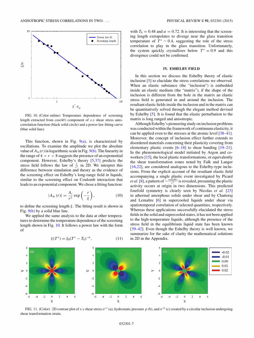
FIG. 10. (Color online) Temperature dependence of screeninglength extracted from cos(4θ ) component of x-y shear stress auto-correlation function (black solid circle) and a power law fitting curve(blue solid line).

This function, shown in Fig. 9(a), is characterized byoscillations. To examine the amplitude we plot the absolutevalue of A4c(r) in logarithmic scale in Fig. 9(b). The linearity inthe range of 4 < r < 8 suggests the presence of an exponentialcomponent. However, Eshelby’s theory [5,37] predicts thestress field follows the law of 1

r2 in 2D. We interpret thisdifference between simulation and theory as the evidence ofthe screening effect on Eshelby’s long-range field in liquids,similar to the screening effect on Coulomb interaction thatleads to an exponential component. We chose a fitting function:

|A4c (r)| = Ac

r2exp

(− r

ξ

), (10)

to define the screening length ξ . The fitting result is shown inFig. 9(b) by a solid blue line.

We applied the same analysis to the data at other tempera-tures to determine the temperature dependence of the screeninglength shown in Fig. 10. It follows a power law with the formof

ξ (T ∗) = ξ0(T ∗ − T0)−α, (11)

with T0 = 0.48 and α = 0.72. It is interesting that the screen-ing length extrapolates to diverge near the glass transitiontemperature of T ∗ ∼ 0.4, suggesting the role of the stresscorrelation to play in the glass transition. Unfortunately,the system quickly crystallizes below T ∗ = 0.9 and thisdivergence could not be confirmed.

IV. ESHELBY FIELD

In this section we discuss the Eshelby theory of elasticinclusion [5] to elucidate the stress correlations we observed.When an elastic substance (the “inclusion”) is embeddedinside an elastic medium (the “matrix”), if the shape of theinclusion is different from the hole in the matrix an elasticstress field is generated in and around the inclusion. Theresultant elastic fields inside the inclusion and in the matrix canbe quantitatively solved through the elegant method devisedby Eshelby [5]. It is found that the elastic perturbation to thematrix is long ranged and anisotropic.

Although Eshelby’s pioneering study on inclusion problemswas conducted within the framework of continuum elasticity, itcan be applied even to the stresses at the atomic level [38–41].Moreover, the concept of inclusion effect further extends todisordered materials concerning their plasticity covering fromelementary plastic events [6–18] to shear banding [19–21].In the phenomenological model initiated by Argon and co-workers [15], the local plastic transformations, or equivalentlythe shear transformation zones noted by Falk and Langer[16,22], are considered analogous to the Eshelby-type inclu-sions. From the explicit account of the resultant elastic fieldaccompanying a single plastic event investigated by Picardet al. [8], a pattern of ∼ cos(4θ )

r2 is revealed, presuming the plasticactivity occurs at origin in two dimensions. This predictedfourfold symmetry is clearly seen by Nicolas et al. [23]in athermal amorphous solids under shear and by Chattorajand Lemaıtre [6] in supercooled liquids under shear viaspatiotemporal correlation of selected quantities, respectively.Whereas these applications successfully elucidated the stressfields in the solid and supercooled states, it has not been appliedto the high-temperature liquids, although the presence of thestress field in the equilibrium liquid state has been known[39–42]. Even though the Eshelby theory is well known, wesummarize for the sake of clarity the mathematical solutionsin 2D in the Appendix.

FIG. 11. (Color) 2D contour plot of x-y shear stress σ s1 (a), hydrostatic pressure p (b), and σ s2 (c) created by a circular inclusion undergoingshear transformation strain.

032301-7

BIN WU, TAKUYA IWASHITA, AND TAKESHI EGAMI PHYSICAL REVIEW E 91, 032301 (2015)

FIG. 12. (Color) The stress fields induced by a circular inclusion suffering from principal transformation strain. The arrangement of panelsis identical to that of Fig. 11.

A. Stress distribution

We first illustrate the anisotropic nature of the stress fieldsinduced by a circular inclusion in 2D. In the examples weassume the radius of the inclusion, a = 0.5, shear modulusμ = 1, Possion’s ratio ν = 0.3, and that the center of theinclusion is placed at the origin of the coordinates.

For the case of pure shear transformation strain, i.e., εT12 =

−0.1 and εT11 = εT

22 = 0, the calculated stress fields are shownin Fig. 11 in the form of two-dimensional contour plots. Thecolor scheme is again set to highlight the far field. Figure 11(a)demonstrates the x-y shear stress σ s1, (b) hydrostatic pressurep, and (c) σ s2. The figures clearly show the symmetry of thefields. The shear stress field has eight lobes that amount to two4θ components, where cos(4θ) < 0 parts carry positive valueswhile cos(4θ ) > 0 parts assume negative values. It is obviousthat the sign of the two components would switch if εT

12 turnspositive. Moreover, the x-y shear stress inside the inclusion isuniform and positive in this specific example. Panels (b) and(c) also manifest evident anisotropicity while the hydrostaticpressure field is rather partitioned into four divisions and σ s2

is essentially a rotating shear stress field anticlockwise to themoduli of π

8 .The Eshelby fields for the case of hydrostatic transforma-

tion strains, i.e., εT12 = 0 and εT

11 = εT22 = −0.1, are presented

in Fig. 12. It is readily recognizable that panel (a) in Fig. 12 isidentical to panel (b) in Fig. 11. Panels (b) and (c) suggest σxx

and σyy in the matrix carry the same magnitude yet oppositesign, and both exhibit the cos(2θ ) pattern. Moreover, the σ s2

field can be again obtained by rotating σ s1 anticlockwise butto the degree of π

4 . The red disk in the center of panel (b)indicates uniform and positive hydrostatic pressure inside theinclusion.

B. Stress correlation in liquids

The similarity of the patterns in Fig. 3 [Fig. 5(a)] and inFig. 11(a) is obvious, except for the oscillation with r . AlsoFigs. 5(b) and 11(b), and Figs. 5(c) and 11(c) share the samesymmetry. The same applies to Figs. 6 and 12. Thus clearlythe angular dependence of the stress correlations in the liquidstate is explained in terms of the Eshelby’s inclusion model.The oscillation with r is related to the PDF and the discretenature of the atomic structure. In the case of the x-y shearstress autocorrelation it is related to the derivative of the PDF

as shown in Fig. 7. For other cases the oscillation is directlyrelated to the pair correlation function as shown in Fig. 8.

V. CONCLUSIONS

A liquid behaves like a solid at a short time scale. Thereforeit can support the elastic stress field for a short time. Thisresults in the stress correlations in the liquids, which contributeto the viscosity. So far, however, only the isotropic stresscorrelations have been studied. In this article we extendedour research into the anisotropic stress correlations. We foundthat the spatial correlations of the atomic-level stresses sharethe same symmetry with the stress fields in the matrix inthe Eshelby’s inclusion model. Specifically, the x-y shearstress autocorrelation function exhibits the familiar fourfoldsymmetry, the correlation of hydrostatic pressure of oneparticle and x-y shear stress of the others characterizes acos(2θ ) symmetry, and so forth. In our view, these long-rangeanisotropic correlation functions indicate the existence of theEshelby-type inclusion effect in the simulated 2D Yukawaliquids. In the Eshelby model the stress field is generated bythe mismatch in shape between the inclusion and the hole in thematrix. In the present case the atomic-level stress is caused bythe mismatch between the shape of the atom (spherical) and thehole in the nearest neighbor shell. The shear stress is generatedwhen the nearest neighbor shell has an elliptic distortion, andthe pressure occurs when the size of the atom and that of thenearest neighbor hole are not the same [39–41,43,44].

However, we found that the amplitude of the anisotropiccomponent of the x-y shear stress autocorrelation functiondoes not follow Eshelby’s prediction of 1

r2 but has addi-tional exponential decay with distance. This difference canbe perceived as a screening effect that has temperaturedependence. The relevant screening length appears to followa power law, diverging at a temperature close to the glasstransition temperature, suggesting a possible role for thestress correlation to play in the glass transition phenomenon.This issue, however, requires further study in the supercooledtemperature range.

It is also of interest to see if the strong stress correlationsseen here in 2D are also present in 3D. We have collectedsome preliminary results on 2D and 3D liquids interactingvia modified Johnson potential [45], and similar results are

032301-8

ANISOTROPIC STRESS CORRELATIONS IN TWO- . . . PHYSICAL REVIEW E 91, 032301 (2015)

obtained. However, more detailed studies are required toanswer this question more definitively.

ACKNOWLEDGMENTS

The authors thank J. S. Langer, J. R. Morris, and J.Bellissard for useful discussions. This research has beensupported by the U.S. Department of Energy, Office ofSciences, Basic Energy Sciences, Materials Sciences andEngineering Division.

APPENDIX: MATHEMATICAL SOLUTIONS OF THEESHELBY PROBLEM IN 2D

Here we discuss two distinct methods of solving the two-dimensional circular inclusion problems. The simplest casesof homogeneous, isotropic, and infinite matrix embedding aninclusion that shares the same elastic moduli are consideredhere. Furthermore, there is neither external loading nor bodyforce. Hence the elastic field inside the inclusion and matrix

is exclusively determined by the transformation strain of theinclusion εT and consequent elastic responses.

The first method can be deemed as the special cases ofEshelby’s [5] original approach in three dimensions underplane strain condition. In this condition, the inclusion hasa cylindrical shape with its axis of symmetry lying alongthe z axis and being infinitely long. In addition, if thecomponents of transformation strains that are related to thez direction, i.e., εT

xz, εTyz, and εT

zz, are zero, then the elasticcondition on the cross-sectional plane is equivalent to thedesired two-dimensional counterpart. In practice, a prolatespheroidal inclusion with its polar axis extending over severalorders of magnitude larger than the equatorial diameter isalready a reasonable approximation of plane strain condition.Therefore, the strain field on the short semiaxis plane can beacquired from derivatives of displacements through numericalintegration either using Eq. (A1) or Eq. (A2). With theadvent of powerful computational resources and sophisticatednumerical calculations recipes, such as finite element method,these integrations are no longer formidable tasks.

ui,m(r) = − 1

16πμ(1 − ν)

∫dS(

−→r ′ )

nk

|−→r − −→r ′ |3

σTkj

{4(1 − ν)(xm − x ′

m)δij − (xj − x ′j )δim − (xi − x ′

i)δjm

− (xm − x ′m)δij + 3

1

|−→r − −→r ′ |2

(xm − x ′m)(xi − x ′

i)(xj − x ′j )

}, (A1)

ui,m(r) = 1

16πμ(1 − ν)

∫dV (

−→r ′ )

σTkj

|−→r − −→r ′ |3

{(1 − 2ν)[(δmk − 3lklm)δij + (δmj − 3lmlj )δik]

− (δmi − 3lmli)δjk + 3[lj lkδim + li lkδjm + li lj δkm − 5li lj lklm]

}. (A2)

Equation (A1) integrates over the surface of the inclusion,

which is the assembly of−→r ′ . Indices in subscripts denote

any one of three Cartesian components: δ, Kronecker deltafunction; μ, shear modulus; υ, Poisson’s ratio; σT , stresscalculated from transformation strain elastically via Hook’s

law; and n, unit normal vector of surface element dS(−→r ′ ).

With employment of Einstein’s notation, the repeated indicessuggest summation, e.g., xixi = x1x1 + x2x2 + x3x3, and anindex preceded by a comma requires derivative operation onthe specified direction, e.g., ui,m = ∂ui

∂xm. Applying Gauss’s

theorem to Eq. (A1) gives rise to Eq. (A2) that integratesover the volume of the inclusion. l represents the unit

vector starting from volume element dV (−→r ′ ) to the point of

interest r .Comparing to degenerating solutions derived in three

dimensions into a 2D version, complex variable formalismis generally more favorable for the plane theory of elasticity.Details concerning this method can be found in Refs. [46,47].In this formalism, each point on the plane is represented byx = x1 + ix2, where i2 = −1, and the corresponding elasticfield can be completely mapped out via two biharmonic

functions of x, e.g., φ(x) and ψ(x), through the followingrelationships:

σ11(x) + σ22(x) = 4Re{φ′(x)}, (A3)

σ22(x) − σ11(x) + 2iσ12(x) = 2{xφ′′(x) + ψ ′′(x)}, (A4)

2μ(u1 + iu2) = κφ(x) − xφ′(x) − ψ ′(x), (A5)

where a prime corresponds to differential operation withrespect to x while double primes mean two times of suchprocedures. Moreover, a bar implies complex conjugateoperation, Re indicates taking the real part of the object, andκ equals either 3 − 4υ under plane strain condition or 3−υ

1+υin

the condition of plane stress.Within this framework, Jaswon and Bhargava [37] un-

raveled Eshelby’s inclusion problems in two dimensions.The solutions were given separately for an elliptic inclu-sion suffering from either pure principal or shear trans-formation strains. In the event of a circular inclusion, therefined φ(x) and ψ ′(x) valid for the matrix are presentedbelow.

032301-9

BIN WU, TAKUYA IWASHITA, AND TAKESHI EGAMI PHYSICAL REVIEW E 91, 032301 (2015)

For principal pressure condition, i.e., εT12 = 0:

φ (x) = μa2

(κ + 1) x

(εT

11 − εT22

), (A6)

ψ ′ (x) = − 2μa2

(κ + 1) x

(εT

11 + εT22

) + μa4

(κ + 1) x3

(εT

11 − εT22

).

(A7)

For shear stress condition, i.e., εT11 = εT

22 = 0:

φ (x) = i2μa2

(κ + 1) xεT

12, (A8)

ψ ′ (x) = i2μa4

(κ + 1) x3εT

12, (A9)

where a is the radius of the inclusion.

[1] J.-P. Hansen and I. R. McDonald, Theory of Simple Liquids, 3rded. (Academic Press, Amsterdam, 2006).

[2] T. Egami, K. Maeda, and V. Vitek, Philos. Mag. A 41, 883(1980).

[3] V. A. Levashov, J. R. Morris, and T. Egami, Phys. Rev. Lett.106, 115703 (2011).

[4] M. P. Allen and D. J. Tildesley, Computer Simulation of Liquids(Oxford University Press, New York, 1987).

[5] J. D. Eshelby, Proc. R. Soc. London, Ser. A 241, 376 (1957).[6] J. Chattoraj and A. Lemaıtre, Phys. Rev. Lett. 111, 066001

(2013).[7] F. Puosi, J. Rottler, and J.-L. Barrat, Phys. Rev. E 89, 042302

(2014).[8] G. Picard, A. Ajdari, F. Lequeux, and L. Bocquet,

Eur. Phys. J. E 15, 371 (2004).[9] C. E. Maloney and A. Lemaıtre, Phys. Rev. E 74, 016118

(2006).[10] A. Tanguy, F. Leonforte, and J. L. Barrat, Eur. Phys. J. E 20, 355

(2006).[11] A. Lemaıtre and C. Caroli, Phys. Rev. E 76, 036104 (2007).[12] M. Tsamados, A. Tanguy, F. Leonforte, and J.-L. Barret, Eur.

Phys. J. E 26, 283 (2008).[13] A. Lemaıtre and C. Caroli, Phys. Rev. Lett. 103, 065501

(2009).[14] A. Le Bouil, A. Amon, S. McNamara, and J. Crassous, Phys.

Rev. Lett. 112, 246001 (2014).[15] V. V. Bulatov and A. S. Argon, Modell. Simul. Mater. Sci. Eng.

2, 167 (1994).[16] J. S. Langer, Phys. Rev. E 64, 011504 (2001).[17] C. Maloney and A. Lemaıtre, Phys. Rev. Lett. 93, 016001

(2004).[18] P. Cao, H. S. Park, and X. Lin, Phys. Rev. E 88, 042404 (2013).[19] R. Dasgupta, H. G. E. Hentschel, and I. Procaccia, Phys. Rev. E

87, 022810 (2013).[20] R. Dasgupta, H. G. E. Hentschel, and I. Procaccia, Phys. Rev.

Lett. 109, 255502 (2012).[21] K. Martens, L. Bocquet, and J.-L. Barrat, Soft Matter 8, 4197

(2012).[22] M. L. Falk and J. S. Langer, Phys. Rev. E 57, 7192 (1998).[23] A. Nicolas, J. Rottler, and J.-L. Barrat, Eur. Phys. J. E. 37, 50

(2014).

[24] P. Schall, D. A. Weitz, and F. Spaepen, Science 318, 1895(2007).

[25] K. E. Jensen, D. A. Weitz, and F. Spaepen, Phys. Rev. E 90,042305 (2014).

[26] S. Plimpton, J. Comput. Phys. 117, 1 (1995).[27] W. K. Qi, S. M. Qin, X. Y. Zhao, and Y. Chen, J. Phys.: Condens.

Matter 20, 245102 (2008).[28] W. K. Qi, Z. Wang, Y. Han, and Y. Chen, J. Chem. Phys. 133,

234508 (2010).[29] H. Yukawa, Proc. Phys.-Math. Soc. Jpn. 17, 48 (1935).[30] W.-R. Chen, L. Porcar, Y. Liu, P. D. Butler, and L. J. Magid,

Macromolecules 40, 5887 (2007).[31] S. Z. Lin, B. Zheng, and S. Trimper, Phys. Rev. E 73, 066106

(2006).[32] B. I. Halperin and D. R. Nelson, Phys. Rev. Lett. 41, 121

(1978).[33] J. M. Kosterlitz and D. J. Thouless, J. Phys. C 6, 1181 (1973).[34] D. R. Nelson and B. I. Halperin, Phys. Rev. B 19, 2457 (1979).[35] A. P. Young, Phys. Rev. B 19, 1855 (1979).[36] S. T. Chui, Phys. Rev. Lett. 48, 933 (1982).[37] M. A. Jaswon and R. D. Bhargava, Math. Proc. Cambridge

Philos. Soc. 57, 669 (1961).[38] T. L. Hoang, A. Arsenlis, H. J. Lee-Voigt, D. C. Chrzan,

and B. D. Wirth, Modell. Simul. Mater. Sci. Eng. 19, 085001(2011).

[39] T. Egami and D. Srolovitz, J. Phys. F: Metal Phys. 12, 2141(1982).

[40] T. Egami, S. J. Poon, Z. Zhang, and V. Keppens, Phys. Rev. B76, 024203 (2007).

[41] T. Egami, Prog. Mater. Sci. 56, 637 (2011).[42] V. A. Levashov, J. R. Morris, and T. Egami, J. Chem. Phys. 138,

044507 (2013).[43] T. Egami and S. Aur, J. Non-Cryst. Solids 89, 60 (1987).[44] V. A. Levashov, T. Egami, R. S. Aga, and J. R. Morris, Phys.

Rev. B 78, 064205 (2008).[45] V. A. Levashov, T. Egami, R. S. Aga, and J. R. Morris, Phys.

Rev. E 78, 041202 (2008).[46] N. I. Muskhelishvili, Some Basic Problems of the Mathematical

Elasticity Theory, 4th ed. (Noordhoff, Leyden, 1977).[47] I. S. Sokolnikoff, Mathematical Theory of Elasticity, 2nd ed.

(McGraw-Hill, New York, 1956).

032301-10